Embed Size (px)
Citation preview

Evaluating Persistence Times in Evaluating Persistence Times in Populations Subject to CatastrophesPopulations Subject to Catastrophes
Ben Cairns and Phil Pollett
Department of Mathematics

Persistence
• Most populations are certain not to persist forever: they will eventually become extinct.
• When is extinction likely to occur?When is extinction likely to occur? We consider such measures as the expected time to extinction (or ‘persistence time’).
• We have developed methods for finding accurate measures of persistence for a class of stochastic population models.

Overview
• Modelling populations subject to stochastic effects:– Birth, death and catastrophe processes.
• Calculating measures of persistence:– Bounded models.– Unbounded models:
• Analytic approaches.• Accurate numerical approaches.

Population Processes
• Populations are subject to a variety of sources of randomness, including:
• There are other sources of randomness (e.g. environmental) but we focus on the above.
• Any model must account for the uncertainty introduced by this stochasticity.
– Survival and reproductionSurvival and reproduction (uncertainty in the survival and reproduction of individuals)
– Catastrophes Catastrophes (events that may result in large, sudden declines in the population by mass death or emigration, often with external causes)

Modelling Populations
• Birth, death and catastrophe processesBirth, death and catastrophe processes, a class of continuous-time Markov chains, are stochastic models for populations.
• As their name suggests, BDCPs incorporate both demographic stochasticity and catastrophic events.
• They are both powerful and simple, allowing arbitrary relationships between population size and dynamics.
• They model discrete-valued populations that are time-homogeneous.

A General BDCP
• BDCPs are defined by rates:– B(i) is the birth ratebirth rate;
i – 2 i – 1 i i + 1
D(i) B(i)
C(i)F(1|i)
C(i)F(2|i)C(i)F(k|i)
– D(i) is the death ratedeath rate;– C(i) is the catastrophe ratecatastrophe rate, with– F( i – j | i ), the catastrophe size distributioncatastrophe size distribution.

A General BDCP
• BDCPs are defined by rates:– B(i) is the birth ratebirth rate;– D(i) is the death ratedeath rate;– C(i) is the catastrophe ratecatastrophe rate, with– F( i – j | i ), the catastrophe size distributioncatastrophe size distribution.

Important Features
• Jumps up limited in size to 1 individual (only births or single immigration).
• This is the most general modelmost general model of its type: it allows any form of dependence of the rates on the current population.
• The population is boundedbounded if it has a ceiling N (then B(i) > 0 for xe < i < N, and B(N) = 0).
• If there is no such N, and B(i) > 0 for all i > xe, the population is ‘unboundedunbounded’.
• A population is quasi-extinct (or functionally extinct) at or below the extinction levelextinction level, xe.

Simulation Example

Persistence: Bounded Pop’ns
• Suppose the population is bounded with ceiling N.
• Extinction is certainExtinction is certain in finite time; persistence times are the solution, T, to
• M = [ qij ], for xe < i, j N. 1 is the unit vector. T = [ Ti ], Ti = persistence time from size i. – If N is not ‘too large’, we can easily find numerical
solutions (e.g. see Mangel and Tier, 1993).

Unbounded Populations
• Unbounded models (ones without hard limits) can still be reasonable population models.
• However, such models could explodeexplode to infinite size in finite time, or never go extinctnever go extinct.
– We would generally want to rule out this kind of behaviour for biological populations.
• If extinction is certain, the persistence times are the minimal, non-negative solution to:

An Unbounded Model
• Suppose there is an overall jump rate, fi, depending only on the current population, i.
• Let the jump size distributionjump size distribution, given that a jump occurs, be the same for all i > 0. Then:
• (Let xe = 0, and deaths be ‘catastrophes’ of size one.)

An Unbounded Model
• Models like this may be useful when:
a)a) Individuals trigger catastrophesIndividuals trigger catastrophes (e.g. epidemics) at rates with forms similar to their birth rates (e.g. by interaction, i(i – 1).)
b)b) Catastrophes are localisedCatastrophes are localised but the population maintains a fairly constant density, so that the catastrophe size distribution is fixed.
• Another advantage: they are quite general and are amenable to mathematical analysis.
• (We find analytic solutions for persistence times and probabilities for this model.)

Unbounded Model: Example
• Suppose the overall jump rate is fi = i –1 and, given a jump occurs,– it is a birth with probability a;– catastrophe size has geometric distribution:
dk = (1-a)(1-p)pk–1, 0 p < 1.
• We show that the persistence times are
if = 1, or
if 1,
whenever p + b/a 1, where b = 1-a, and = 1/.

Unbounded Model: Example
Approximating Persistence
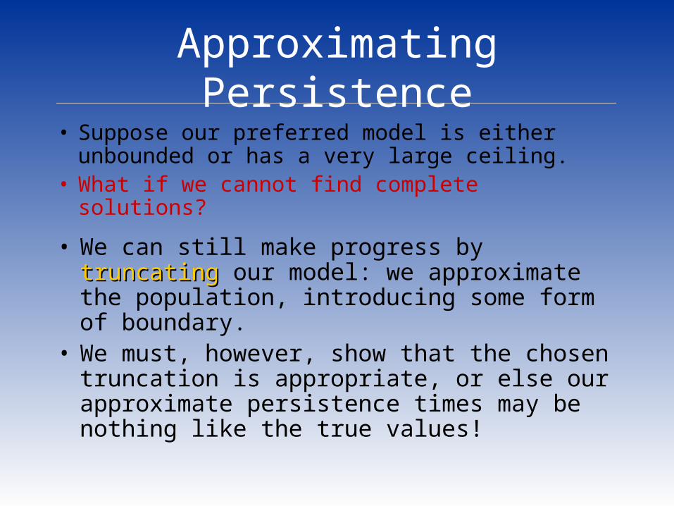
• Suppose our preferred model is either unbounded or has a very large ceiling.
• What if we cannot find complete solutions?
• We can still make progress by truncatingtruncating our model: we approximate the population, introducing some form of boundary.
• We must, however, show that the chosen truncation is appropriate, or else our approximate persistence times may be nothing like the true values!

Approximating Persistence
• Interesting properties of extinction times (expectations, etc.) are all solutions to
Solutions have the form (Anderson, 1991)
where k* = supi > xe [ bi / ai ] ensures this is the minimal,
non-negative solution.

Approximating Persistence• See Anderson (1991) for details of the (fairly simple)
derivation of the sequences {ai} and {bi}. These sequences are unique.
• In our work, we do not use Anderson’s results to calculate persistence times directly, but rather obtain from them a quantitative indicator of the accuracy of a truncation.
• However, could in theory find {ai} and {bi} for xe < i N+1, then let k* kN+1 = bN+1 / aN+1…

Accurate Approximations
• Then
• This will be an accurate approximation provided kN+1 is close to k*, which we can judge in two ways:– Plot kN+1 versus N+1 and look for convergence.– If a plot of kN+2 = kN+2 – kN+1 is linear on log-linear
axes, kN+1 appears to converge geometrically (fast) to k*.

Accurate Approximations
kN+2 = kN+2 – kN+1 approaches 0 geometrically.
kkN+1N+1 appears appears
to converge…to converge…

Absorption vs. Reflection
• Direct use of Anderson’s approach is not satisfying in many cases: it allows the population to become ‘extinct’ by going above N! Then, N+1 is an absorbing boundaryabsorbing boundary.
• In our approach, we take a truncation with a reflecting boundaryreflecting boundary, so that the N is a true ceiling and only states xe correspond to quasi-extinction. We calculate persistence times etc. as for bounded populations, and …
• we use the convergence of ki as an indication of the accuracy of the truncation.

Example: Numerical Solutions
Conclusions
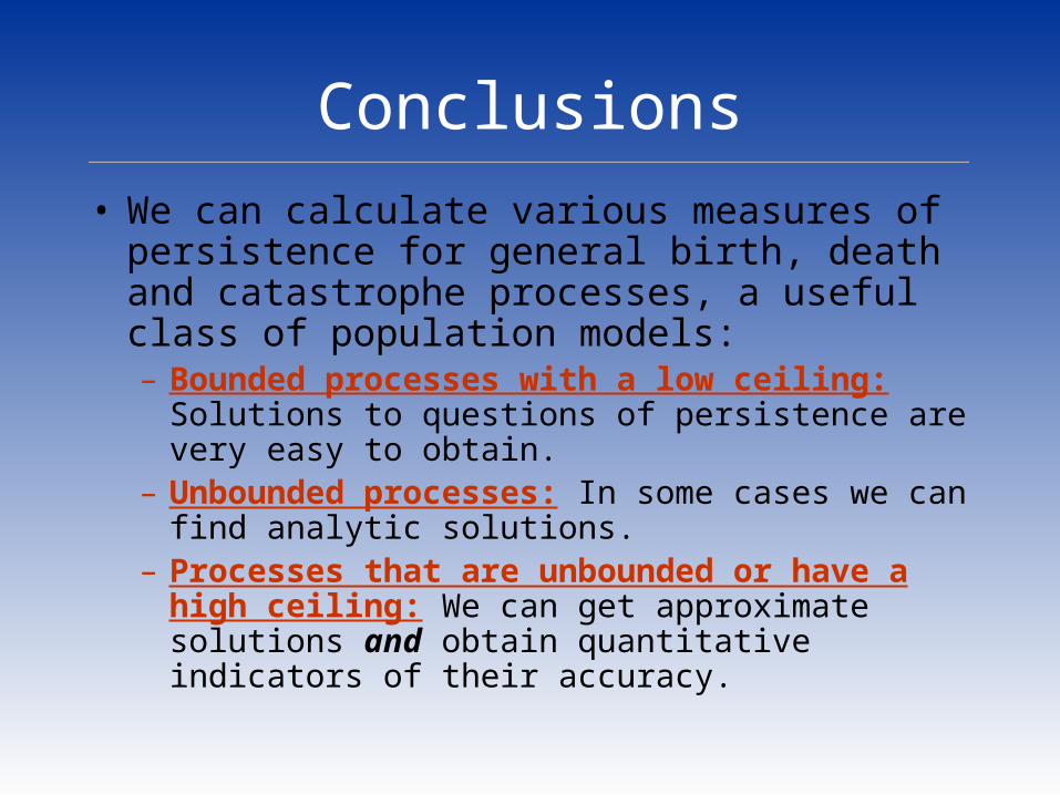
• We can calculate various measures of persistence for general birth, death and catastrophe processes, a useful class of population models:– Bounded processes with a low ceiling:
Solutions to questions of persistence are very easy to obtain.
– Unbounded processes: In some cases we can find analytic solutions.
– Processes that are unbounded or have a high ceiling: We can get approximate solutions and obtain quantitative indicators of their accuracy.

Acknowledgements
• Dr Phil PollettDr Phil Pollett (supervisor and co-author)
• Prof. Hugh PossinghamProf. Hugh Possingham (associate supervisor)
… and the organisers of MODSIM 2003: