Evaluating Scalability Parameters

This is the final online article concerning the concept of application scalability. Here, you will learn how to determine value of the parameters that control scalability.

The previous articles in this series include "Commercial Clusters and Scalability," and "How to Measure and Elephant."

Evaluating ScalabilityParameters:A Fitting End

About the AuthorNeil J. Gunther, M.Sc., Ph.D., is an internationally known computer performance and IT researcher who founded Performance Dynamics in 1994. Dr. Gunther was awarded Best Technical Paper at CMG’96 and received the prestigious A.A. Michelson Award at CMG’08. In 2009 he was elected Senior Member of both ACM and IEEE. His latest thinking can be read on his blog at perfdynamics.blogspot.com

http://www.teamquest.com/pdfs/whitepaper/scalability.pdf

http://www.teamquest.com/pdfs/whitepaper/elephant.pdf

http://www.youtube.com/user/TeamQuestOptimizesIT

http://www.teamquest.com/blog

http://twitter.com/TeamQuest_Corp

http://www.linkedin.com/groups?home=&gid=984207&trk=anet_ug_hm

1. Let’s Review

The key points that I made in the previous columns can be summarized as:

• Scalability is not a number, it’s a function. Such a function is the Super-Serial model.• The Super-Serial model is a concave1 function that permits the possibility of a capacity

maximum. (unlike Amdahl Scaling)• The independent variable is either the processor configuration C(p) or the user load C(N)• The shape of the function is controlled by two parameters: σ and λ.• The σ parameter is a measure of the level of contention in the system (e.g., waiting on

a database lock)• The λ parameter is a measure of the level of coherency in the system (e.g., cache-miss

ratio)• For the case where λ = 0, the Super-Serial model reduces to Amdahl’s Law.• Amdahl’s Law has a queueing interpretation viz, worst-case bound with all N users

enqueued.

It’s interesting to note that scalability (particularly application scalability) is currently a hot topic (See for example: [Apache 2000], [Oracle9i 2001], [Trends 2001], [SQLServer 2000]), yet few authors are able to quantify the concept. The version of the Super-Serial model most appropriate for assessing application scalability (cf. [ Gunther 2000]) is given by:

where C(N) is defined as the Capacity or normalized throughput:

at N users.

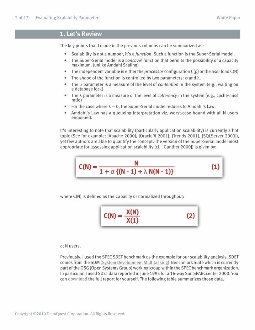
Previously, I used the SPEC SDET benchmark as the example for our scalability analysis. SDET comes from the SDM (System Development Multitasking) Benchmark Suite which is currently part of the OSG (Open Systems Group) working group within the SPEC benchmark organization. In particular, I used SDET data reported in June 1995 for a 16-way Sun SPARCcenter 2000. You can download the full report for yourself. The following table summarizes those data.

2 of 17 Evaluating Scalability Parameters White Paper

Copyright ©2010 TeamQuest Corporation. All Rights Reserved.

C(N) = (1)N1 + σ {(N - 1) + λ N(N - 1)}

C(N) = (2)X(N)X(1)

http://www.spec.org/osg/sdm91/

http://www.spec.org/osg/sdm91/results/res9506/

White Paper


Table 1: SPEC SDET Benchmark on a 16-way Sun SC2000

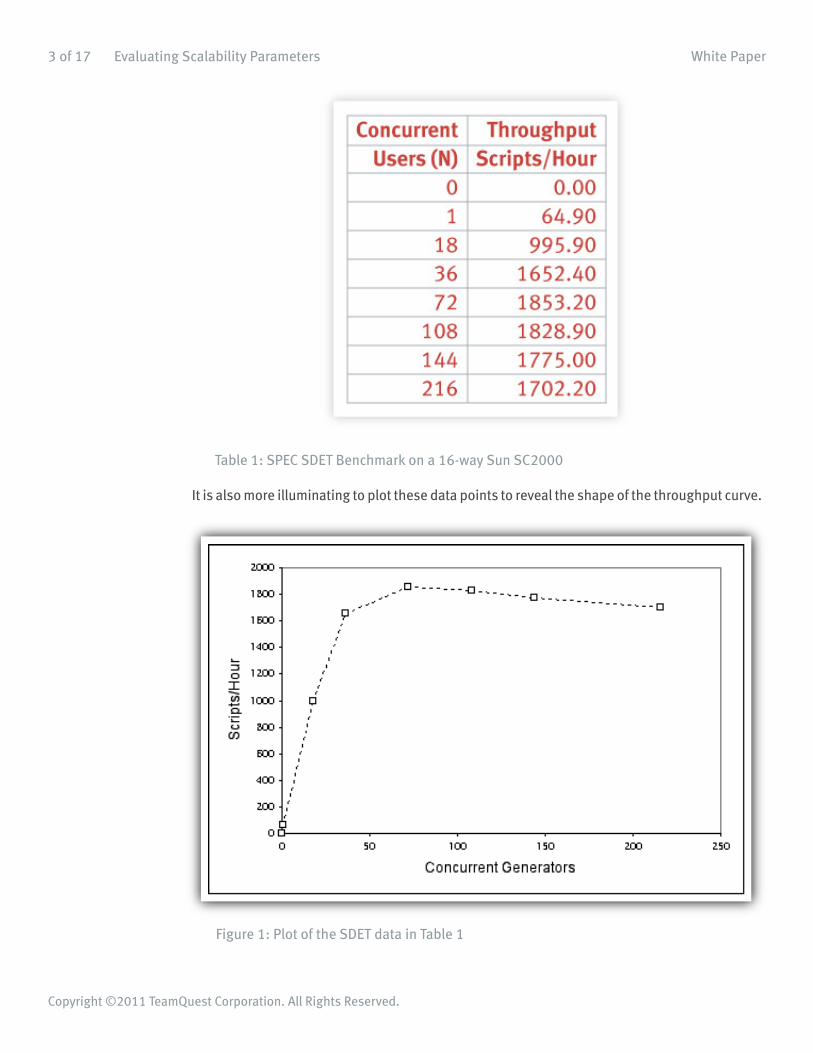
It is also more illuminating to plot these data points to reveal the shape of the throughput curve.

Figure 1: Plot of the SDET data in Table 1

3 of 17 Evaluating Scalability Parameters

White Paper


The most significant features of this benchmark are:

• Reporting a single performance metric is not sufficient. The complete throughput characteristic must be displayed.

• The throughput has a maximum (at 1853.20 scripts/hour).• The maximum throughput occurs at 72 generators (i.e., emulated users).• There are 3 data points on each side of the maximum throughput (part of the SPEC-SDM

run rules).• Beyond the maximum, throughput becomes retrograde!

This makes SDET a very suitable candidate for analysis using our Super-serial capacity model (1) and to that end I will now show you how to evaluate the σ and λ parameters from this data. Notice that it would be a good deal more difficult to construct a queueing model with this throughput characteristic. The basic steps in the calculation of σ and λ can be summarized as follows:

1. Measure the throughput2 X(N) as a function of load (N). (SDET provides that already).2. Calculate the capacity ratio C(N), the efficiency C/N, and its inverse N/C from the data.3. Calculate the Quadratic transform. (Explained below).4. Perform a Quadratic regression fit on the transformed data.5. Calculate the parameters {σ, λ} from the regression coefficients {a, b, c}.6. Use the values of σ and λ to predict the complete scalability function, C(N).

These steps are easily carried out in a spreadsheet (e.g., MS EXCEL [Stats for Managers 1999]).

Figure 2: Example spreadsheet

An example spreadsheet is shown in Figure 2. Now, let's examine each of these steps in detail.


White Paper


2. Capacity Ratios

Referring back to the benchmark data in Table 1, the first thing to do is to calculate the relative capacity C(N) for each of the measured loads (N). We see that the single user throughput was measured at X(1) = 64.90 scripts/hour. Therefore,

which follows from the definition in equation (2). Similarly, for N = 216 users we have:

All the intermediate C(N) values can be calculated in the same way. Additionally, we can calculate the efficiency (C/N) and it's inverse (N/C) for each of the measured user loads.

Table 2: Relative capacity, efficiency, and inverse efficiency

The complete set of entries appears in Table 2. We are now in a position to set up the corresponding data for Regression Analysis [Stats for Managers 1999]. Some readers may already be familiar with the most common form of statistical regression that uses a ''Linear Least Squares'' fit. The technique we shall use here is a form of nonlinear regression.

N1183672108144216

C1.0015.3525.4628.5528.1827.3526.23

C/N1.000.850.710.400.260.190.12

N/C1.001.171.412.523.835.278.24


White Paper


3. Regression Equation

Unfortunately, due to the nature of the equation, we cannot perform a regression analysis directly on the Super-serial model in equation (1). We can, however, do regression on a transformed version of the Super-serial model. The transformed version of C(N) is arrived at using the following steps:

3.1 Efficiency Form

First, we divide both sides of equation (1) by N to give:

This is equivalent to an expression for the relative efficiency.

3.2 Inverted Efficiency

Second, we simply invert both sides of equation (3) to produce:

This form is more useful because the right-hand side of equation (4) is now a simple second-degree polynomial (a parabola), and EXCEL (as well as most other statistical packages) can easily fit such a parabola or quadratic equation:

with coefficients: a, b, and c. This is the nonlinear part of the regression referred to earlier.

3.3 Constrained Parameters

Finally, we need to make the connection between the polynomial (5) coefficients {a, b, c} and the parameters {σ, λ} of the Super-serial model (1). Note, however, that we have more coefficients than we have parameters. Another way of saying this is, we have more degrees of freedom in the fitting equation than the Super-serial model allows. Since we are not simply

= (3)CN

11 + σ{(N - 1) + λN(N - 1)}

= 1 + σ{(N - 1) + λN(N - 1)} (4)NC

y = (5)ax2 + bx + c


White Paper


doing a ''curve fitting'' exercise, we need to constrain the regression in such a way that:

• There are only 2 coefficients• Their values are always positive

This can most easily be accomplished by adjusting the inverted equation (4) using the following variable substitutions:

Y = (N/C) - 1

and

X = (N - 1)

Then, equation (4) can be rearranged to produce:

Notice how it looks very much like equation (5) with the exception that there is no constant equivalent to the c coefficient. In other words, the match up between this constrained equation (6) and the quadratic polynomial (5) is obtained by setting the intercept to be zero (c = 0).

Overall, these transformations simply mean that we must perform the regression analysis on the new variables X and Y defined above.

Table 3: Quadratic Transform

N-10173571107143216

(N/C)-10.000.170.411.522.834.277.24


y = (5)ax2 + bx + c

White Paper


The values corresponding to these variables are collected in Table 3.The relationship between the Super-serial parameters {σ, λ} and the quadratic coefficients {a, b, c} is given by:

and

Notice that the c coefficient plays no role in determining σ and λ. Having secured these particulars, we are now in a position to determine the values of the {a, b} coefficients using the SPEC SDET benchmark data.

4. Regression Analysis

The simplest way to perform the regression fit in EXCEL is to make a scatter plot of the transformed data in Table 3. Once you have made the scatter plot, go to the Chart menu item in EXCEL and choose Add Trendline. This option will then present you with a dialog box with 2 tabs:

1. Type 2. Options

The Type tab allows you to select the type of regression curve you would like to fit to the data. Select Polynomial and ratchet the Degree setting until it equals 2. This corresponds to the quadratic fit we desire.

σ = (8)aλ

λ = (7)ab - a


White Paper


Figure 3: Dialog box for EXCEL Trendlines

Now go to the Options tab shown in Figure 3 and tick each of the checkboxes:1. Set intercept 02. Display equation on chart3. Display r-squared value on chart

The first checkbox forces the c coefficient to be zero (as we require). The second and third checkboxes will cause the {a, b} coefficients to be displayed along with the R2 value. R2 is affectionately known to statisticians as the Coefficient of Determination but you can read it as the percentage of variability in the data that is accounted for by the Super-serial model.


White Paper


Figure 4: Regression fit to the parabolic transform

The result of these steps in EXCEL is shown in figure 4. We see the transformed data along with the fitted quadratic curve (the dashed parabola), as well as the full quadratic equation and the R2 value as we requested. The {a, b, c} coefficients are collected in the following table.

Table 4: Regression coefficients for the Quadratic Transform

In this case, R2 = 99.61% which means that less than 1% is unaccounted for by our scalability model. This is a statistical definition of ''Not bad, dude!''

Regressionabc

Coefficients8.00E-050.01700.0000


White Paper


Table 5: Scaling Parameters

The scalability parameters σ and λ can now be calculated by plugging the values from Table 4 into equations (8) and (7) above. The results are collected in Table 5. This ends the regression analysis. We are now in a position to generate the entire scaling curve using the Super-serial model in equation (1).

Figure 5: Super-serial model of SDET benchmark data

SuperParameter

σλ

Nmax

SerialValues0.01690.0047

111


White Paper


The resulting scalability curve (dashed line) is compared to the original measurements in Figure 5. Several remarks can be made:

1. σ, the contention parameter, is less than 2% (1.69% but let's not get carried away with precision).

2. λ, the coherency parameter, is less than 0.5% (0.47% to be exact).3. Below the measured peak load of 72users, serial contention is slightly less than predicted

by the model.4. Above the measured peak load of 72 users, coherency is slightly worse than predicted

by the model.

Hopefully, these steps have convinced you that the Super-serial model is not only sound conceptually, but can be used empirically to analyze real performance data.

5. Less Than the Full Quid

Of course, you may be thinking that we have done quite well only because the data set corresponds to a complete throughput curve (above and below the peak load). What happens to the regression method when there is less data than that provided by the SPEC benchmark? Let's consider some more typical cases:

1. Measurements below the peak2. Missing an X(1) measurement3. Measurements around the peak.

5.1 Below the Peak

Suppose we only had 4 data points below the knee of the SDET peak as shown in the following table.

Table 6: SPEC SDET Benchmark low contention data

ConcurrentUsers (N)

1183672

ThroughputScripts/Hour

64.90995.901652.401853.20


White Paper


This corresponds to the low-load or low-contention region. Recall from earlier remarks that 4 data points is the minimum requirement for meaningful regression.

Table 7: Low Load Parameters

The σ value is higher than the original regression analysis by a factor of two. The λ value is higher than the original regression analysis by a factor of three. The estimate of the peak load is closer, however, and the R2 is slightly higher because there are fewer data points to fit.

5.2 Missing X(1) Measurement

If we followed a similar regression analysis using the Amdahl model (λ = 0) instead of the Super-serial model, we would find a value of σ = 0.031 (R2 = 0.962) which is in very good agreement with the value of σ = 0.033 determined by our previous queueing theory analysis. This is an encouraging confirmation of the validity of our regression modeling approach.

The calculations can be found in a spreadsheet which you can download from the Performance Dynamics Tools directory.

The X(1) value can be estimated using this simpler 1-parameter Amdahl model. This makes sense because close to the origin (N = 0), the models are essentially identical. The details of how this is done are presented in my classes [Gunther 2001].

5.3 Around the Peak

Next, suppose we only had 3 data points around the knee of the SDET peak as shown in the following table. Three data points is less than the desired minimum requirement but it does not prohibit doing the analysis.

SuperParameter

σλ

NmaxR2


680.9987



http://www.perfdynamics.com/Tools/sdmcalc.xls

White Paper


Table 8: SPEC SDET Benchmark knee

Note also that we are missing the X(1) data point needed to calculate the capacity ratios like those in Table 2. We can use our regression technique on the Amdahl model (λ = 0) to estimate it.

Table 9: Knee Parameters

The σ value is much higher than the original regression analysis whereas the λ value is much lower than the original regression analysis by a factor of three. The R2 is the highest because there are even fewer data points to fit.

Plotting the throughput curves for each of these examples is left as an exercise for the reader.

ConcurrentUsers (N)

3672108

ThroughputScripts/Hour

1652.401853.201828.09

SuperParameter

σλ

NmaxR2


1410.9991


White Paper


6. Summary

What should you walk away with from these online columns about scalability?

First, scalability has to be characterized as a function. The function presented here is the effective capacity C(*) based on the normalized throughput-and the throughput is a completely measurable quantity. When you are trying to size [SQLServer 2000] processors for a server, the appropriate independent variable is the number of processors (p). The processor context was used to present the basic concept of scalability in Part 1. For the special case of λ = 0, we showed that C(p) reduces to the well-known Amdahl's Law [Gunther 2000]; denoted CA(p).

Conversely, in Part 2, we showed that Amdahl's Law has a queueing theory interpretation when p is replaced by N; the number of active users on the system. It represents the extreme case where all N requests are either ''thinking'' or enqueued for service. In this sense Amdahl's Law, as expressed in CA(N), can be thought of as a worst-case bound on application capacity. We applied this bound to the analysis of some real-world benchmark data and showed how it is possible to drive out more performance information than would seem apparent from the measured data. This additional information was summarized in the section entitled, The Elephant's Dimensions at the end of Part 2.

The only thing missing from the previous columns was the determination of the modeling parameters σ and λ. That has been the focus of this column. We used (nonlinear) Regression Analysis [Stats for Managers 1999] on the application form of the Super-serial model in equation (1). The application form, C(N), is most appropriate for analyzing benchmark data.

The basic steps in extracting the scalability parameters can be summarized as follows:

1. Measure the throughput X(N) as a function of load (N).2. A sparse data sample (more than 4 loads) is OK.3. Calculate the capacity ratio C(N), the efficiency C/N , and its inverse N/C from the data.4. Calculate the Quadratic transform.5. Perform a regression fit on the Quadratic transform.6. Calculate the parameters {σ, λ} from the regression coefficients {a, b, c}.7. Use the values of σ and λ to predict the complete scalability function, C(N).

The main point of modeling smaller data samples at the end of this article was to give you some confidence that the regression method still works although, as you would expect, the predictions may be less accurate than those for a more complete data sample.


http://www.teamquest.com/pdfs/whitepaper/scalability.pdf


White Paper


References

[Apache 2000] Apache.org How-To on: ''Scalability - Load--Balancing - Fault tolerance.''

[Oracle9i 2001] See Larry Ellison defend against BEA performance claims ... (Nothing like a good benchmarketing war to start the morning!)

[Gunther 2000] Gunther, N. J., The Practical Performance Analyst, iUniverse.com Inc. 2000.

[Gunther 2001] Gunther, N. J., Lecture notes for Guerilla Capacity Planning class.

[SQLServer 2000] Network Fusion online article: ''A Look at Eight-way Server Scalability.'' Take special note of the throughput curves.

[Stats for Managers 1999] Statistics for Managers Using Microsoft EXCEL, Levine, D., Berenson, M., Stephan, D., New Jersey: Prentice-Hall (1999).

[Trends 2001] Performance Engineering: State of the Art and Current Trends, (Eds.) Dumke, R., Rautenstrauch, C., Schmietendorf, A., Scholz, A., Springer Lecture Notes in Computer Science, # 2047. Heidelberg: Springer-Verlag (2001).

Footnotes1 The terms concave and convex have strict mathematical definitions. Here, concave refers to the fact that the function C(N) has a unique maximum while convex means there is a unique minimum. If you get these terms back-to-front don't worry, I do too. In contradistinction, a concave lens is ''bowl'' shaped and caves in. It doesn't cave out!

2 You do not need to have a data set as encompassing as the SDET benchmark. Fewer measured loads can be analyzed using the above capacity model (1), although the projections may not be as accurate as a denser data set. In any event, it is advisable to have 4 or more load points. This is to offset the fact that it is always possible to fit a parabola through 2 arbitrary points. Including another measurement (for a total of 3 points) might also produce an R2 = 1.0, which is not very convincing. Hence, 4 data points should be considered the minimal set. The ability to make scaling projections based on fewer measured load points can also help to keep the time and expense of the measurement process under control.


http://www.perfdynamics.com/Classes/Outlines/guerilla.html.

http://www.networkworld.com/reviews/2000/0703rev2.html

http://www.networkworld.com/reviews/2000/0703rev2.html

TeamQuest Corporation

www.teamquest.com

AmericasOne TeamQuest WayClear Lake, IA 50428USA+1 641.357.2700+1 [email protected]

Europe, Middle East and AfricaBox 1125405 23 GothenburgSweden+46 (0)31 80 95 00United Kingdom+44 (0)1865 338031Germany+49 (0)69 6 77 33 [email protected]

Asia Pacific6/F CNT Commercial CentreNo. 302 Queen's Road, CentralHong Kong, SAR+852 [email protected]

Copyright ©2011 TeamQuest CorporationAll Rights Reserved

TeamQuest and the TeamQuest logo are registered trademarks in the US, EU, and elsewhere. All other trademarks and service marks are the property of their respective owners. No use of a third-party mark is to be construed to mean such mark’s owner endorses TeamQuest products or services.The names, places and/or events used in this publication are purely fictitious and are not intended to correspond to any real individual, group, company or event. Any similarity or likeness to any real individual, company or event is purely coincidental and unintentional.NO WARRANTIES OF ANY NATURE ARE EXTENDED BY THE DOCUMENT. Any product and related material disclosed herein are only furnished pursuant and subject to the terms and conditions of a license agreement. The only warranties made, remedies given, and liability accepted by TeamQuest, if any, with respect to the products described in this document are set forth in such license agreement. TeamQuest cannot accept any financial or other responsibility that may be the result of your use of the information in this document or software material, including direct, indirect, special, or consequential damages.You should be very careful to ensure that the use of this information and/or software material complies with the laws, rules, and regulations of the jurisdictions with respect to which it is used.The information contained herein is subject to change without notice. Revisions may be issued to advise of such changes and/or additions. U.S. Government Rights. All documents, product and related material provided to the U.S. Government are provided and delivered subject to the commercial license rights and restrictions described in the governing license agreement. All rights not expressly granted therein arereserved.

Follow the TeamQuest Community at:

mailto:[email protected]?Subject=Gunther: Evaluating Scalability Parameters



http://www.youtube.com/user/TeamQuestOptimizesIT

http://www.teamquest.com/blog

http://twitter.com/TeamQuest_Corp

http://www.linkedin.com/groups?home=&gid=984207&trk=anet_ug_hm

Documents

Evaluating Scalability Parameters