Evaluating Scientific Coverage Strategies for A Heterogeneous Fleet of Marine Assets Using a Predictive Model of Ocean Currents

Andrew Branch1, Martina Troesch1, Selina Chu1, Steve Chien1, Yi Chao2, John Farrara2, Andrew Thompson3

1Jet Propulsion Laboratory, California Institute of Technology 2Remote Sensing Solutions

3California Institute of Technology Correspondence Author: steve.a.chien@jpl.nasa.gov

Abstract Planning for marine asset deployments is a challenging task. Determining the location to where the assets will be deployed involves considerations of (1) location, extent, and evolution of the science phenomena being studied; (2) deployment lo-gistics (distances and costs), and (3) ability of the available vehicles to acquire the measurements desired by science. This paper describes the use of mission planning tools to evaluate science coverage capability for planned deploy-ments. In this approach, designed coverage strategies are evaluated against ocean model data to see how they would perform in a range of locations. Feedback from these runs is then used to refine the coverage strategies to perform more robustly in the presence of a wider range of ocean current settings.

Introduction Study of the ocean is of paramount importance in under-standing the Earth’s environment in which we live. Oceans cover the majority of the Earth’s surface and play a domi-nant role in climate and the Earth’s ecosystems. Space based remote sensing provides great information about ocean dynamics. However, remote sensing infor-mation is generally limited to measuring the ocean surface or the upper layer of the ocean. Ocean models can further augment this information. However, in order to probe the immense volume of the ocean most accurately generally re-quires marine vehicles such as autonomous underwater ve-hicles (AUVs), Seagliders, profiling buoys, and surface ve-hicles sampling in-situ. Deploying and operating these as-sets is very expensive. This means there is a very limited number of marine vehicles compared to the massive size of the ocean. Knowing where the assets should be deployed and operated is very difficult. One strategy is to deploy in-

Copyright © 2016, All rights reserved.

situ assets to study specific scientific features such as fronts, eddies, upwellings, harmful algal blooms, or other features of interest. A typical strategy would be to deploy marine assets to measure transects across the feature of interest at a scale that covers the feature, as well as a baseline signal around the feature. However, asset capabilities (e.g. mobil-ity, endurance) and prevailing ocean currents may render these science goals unachievable. Our project targets auto-matic generation of mission plans for assets to follow these science derived templates. This paper specifically describes the use of this planning technology to assess feasibility of achieving these science templates to support both: deploy-ment design (number of assets, where, which templates to follow) and science template design (how to adjust designed templates to be feasible in settings where they are not likely to succeed in original form). The remainder of this paper is organized as follows. First, we discuss the problem that we are trying to solve and the inputs to that problem that we use, including the predictive ocean model and the types of assets. Then we discuss the approach that we took to solve the problem and the results of that approach. Finally, we discuss what needs to be done next to continue to develop a solution to this problem.

Problem Definition The goal of the path planning software is to develop a plan of control directives that when executed by a marine asset in an actual ocean current field will cause the marine asset to follow a template path relative to an ocean feature of science interest, where a template path is a series of edges between waypoints. An example of a template path can be seen in figure 4. In this case, the templates in the figure are going

from one corner of a 15km x 15km box to the opposite cor-ner. Nominally this path should take 24 hours to complete. Ideally the asset would perfectly follow the line but in reality the asset should follow the line as closely as possible and achieve the endpoint within 0.5 km. There are really two related problems that have differing inputs and outputs but use much of the same search-based algorithm. First, before an actual deployment, it is useful to assess a range of deployment locations and science template coverage strategies. Second, during an actual deployment, we have an actual set of asset locations and the goal is to develop asset directives using a current model that will fol-low the template directed paths in reality.

The Template Assessment and Feasibility Problem The focus of this paper is the pre-deployment assessment of locations and science templates for feasibility. The inputs to this are: (1) a set of template paths, (2) a set of asset mod-els, (3) a planning ocean current model, (4) a nature ocean current model, and (5) a set of evaluation locations. The first template waypoint in this path is the start location for the asset. The asset model determines how the asset will behave when simulating actions in a current model. The planning and nature current models specify ocean currents for x, y, z, and over the relevant proposed deployment domains. The planning and nature models are used to simulate the inaccu-racies of an ocean model with respect to the actual ocean. The planner constructs a set of control actions for the asset that when executed in the lower fidelity model i.e., the plan-ning model, should follow the desired science template. These control actions are then evaluated in the higher fidel-ity model i.e., the nature model, to simulate planning model inaccuracies. This process is repeated over a set of evalua-tion locations. A few assumptions are made in this problem. First, we assume that the discrepancies between the planning and na-ture ocean models are similar to the inaccuracies present be-tween a planning model and the actual ocean during a de-ployment. If this is not the case, then the results are not help-ful when preparing for an actual operational deployment. We also assume a number of things about the asset, namely that the asset motion model is accurate. We also do not model hardware issues such communication failures, GPS failures, and navigation inaccuracies.

Operational Deployment A second related problem is an actual deployment usage problem. In this case we are given a set of template paths asset models, asset locations, and a single ocean current model. The templates and asset models are defined in the same manner as before. In our current approach only one current model is used and we do not evaluate, predict, or model the inaccuracies of the predictive ocean models (see

future work on ensemble modelling). The output produced by the planner will be a series of control actions in the form of directed waypoints called command points, which are distinct from the waypoints that make up the template path. The command points are then used by the assets to navigate. Many of the same assumptions are made in this problem as with the previous one. We assume that the ocean model currents reflect the actual ocean currents. When running the planner, we still assume that there will be no future hardware failures and that the properties for the assets are accurate.

Ocean Model Any cell-based, predictive model with information about ocean currents over multiple depths and an extended period of time could be used for the path planning. Some widely spread ocean models include the Harvard Ocean Prediction System (HOPS) (Robinson 1999), the Princeton Ocean Model (POM) (Mellor 2004), the Regional Ocean Model-ling System (ROMS) (Li et al. 2006), and the Hybrid Coor-dinate Ocean Model (HYCOM) (Chassignet et al. 2007). For our ocean model, we used the Regional Ocean Mod-elling System (ROMS) (Chao et al. 2009; Li el al. 2006; Far-rara et al. 2015). The grid spacing used for our experiment was approximately 3km x 3km and had 14 depths ranging from 0 to 1000m in non-uniform levels. Data was available at 1 hour intervals for a 72-hour period. As stated previously, two different ocean models are used to represent the inaccuracies in predictive ocean models. The ROMS model with the best representation is used as the ocean, this is referred to as the nature model. The second model that is used does 6 days of advanced prediction. This is referred to as the planning model. Fewer days of ad-vanced predication mean a higher fidelity model and thus the planning model is closer to the nature model. The list of inputs used for the planning and nature model can be found in (Troesch et al. 2016b). When simulating the movement of an asset, the closest grid point in the latitude, longitude, and depth dimensions is used. Whenever the asset crosses into the next depth dimen-sion the latitude and longitude information is updated. The time used is the previous hour. For example, in the first hour of operation the information at time index 0 is used. No in-terpolation is done in any dimension.

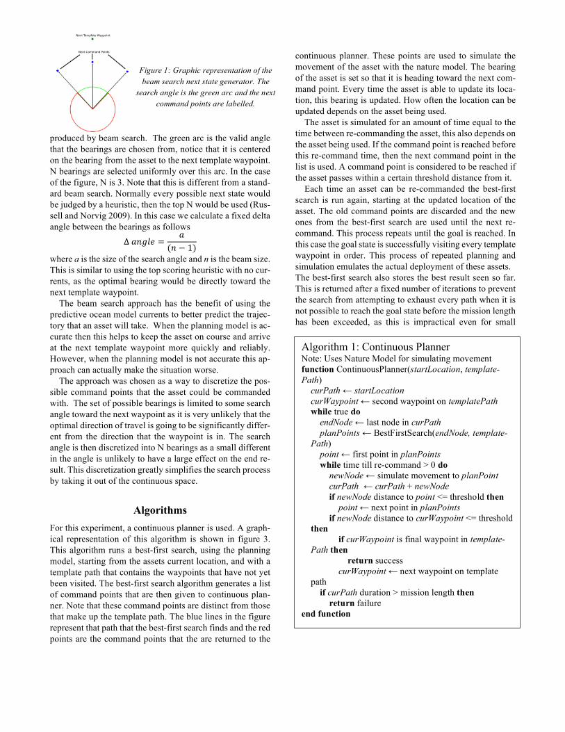
Assets Three different assets are used for this experiment, Seaglid-ers, AUVs, and Wave Gliders. The Seagliders repeatedly profile between the surface and some depth, with a specific bearing (Eriksen et al. 2001). It is only during these profiles where they have any forward movement. If the ocean floor or an obstacle is reached before the profile depth, the asset

will abort that profile and start to ascend. When the Sea-glider is at the surface it is able to update its location using GPS and communicate with the shore. This allows the asset to receive new commands. The dive profile can be seen in figure 1.

The AUVs are much more flexible than the Seagliders in how they move through the water. However, for this exper-iment, they are treated very similar to the Seagliders. They repeatedly profile between the surface and some depth, only moving forward when profiling. The AUV will also avoid the ocean floor by ascending before the profiling depth has been reached. When at the surface, the AUV is able to up-date its location. Communication is done through an acous-tic modem. The final asset is the Wave Glider. The Wave Glider has two components, a float and a set of submerged fins, con-nected by a cable (Manley 2010). As such, the current that affects the asset is not at one single depth. For the purposes of this experiment, the current that the Wave Glider experi-ences is two-thirds the current at the surface and one-third the current at 10m.

Next State Generators Next state generators are used to discretize the problem space. The generators use the properties of each asset, hori-zontal and vertical speed and maximum depth, a planning model, and different heuristics to generate the next states by simulating different actions that the asset can take in the planning model.

Baseline This next state generator serves as the baseline for the ex-periment. Each time an asset is at the surface, the asset ad-justs its heading to the direction of the next template way-point. This is the simplest approach that will allow the asset

to reach the waypoints along the path. As each state only has one neighbor, there is no actual search involved. This ap-proach simulates commanding the assets with only the tem-plate waypoints. This approach has the benefit of not needing an ocean model for an operational deployment. If there is poor corre-lation between the ocean model currents and the actual ocean currents, then this approach would be superior to oth-ers. In addition, there is very little in the way of operator intervention when deployed. Once the waypoints are given to the asset there is no need send any re-commands. The ma-jor downside is the affect the currents can have on the asset. If it is important to precisely follow the template path, then this approach may perform poorly in the presence of cross-currents. This approach was chosen as the baseline for two reasons, the lack of a need for a planning model and the sim-ilarity to the default behavior of the assets when given the list of template points.

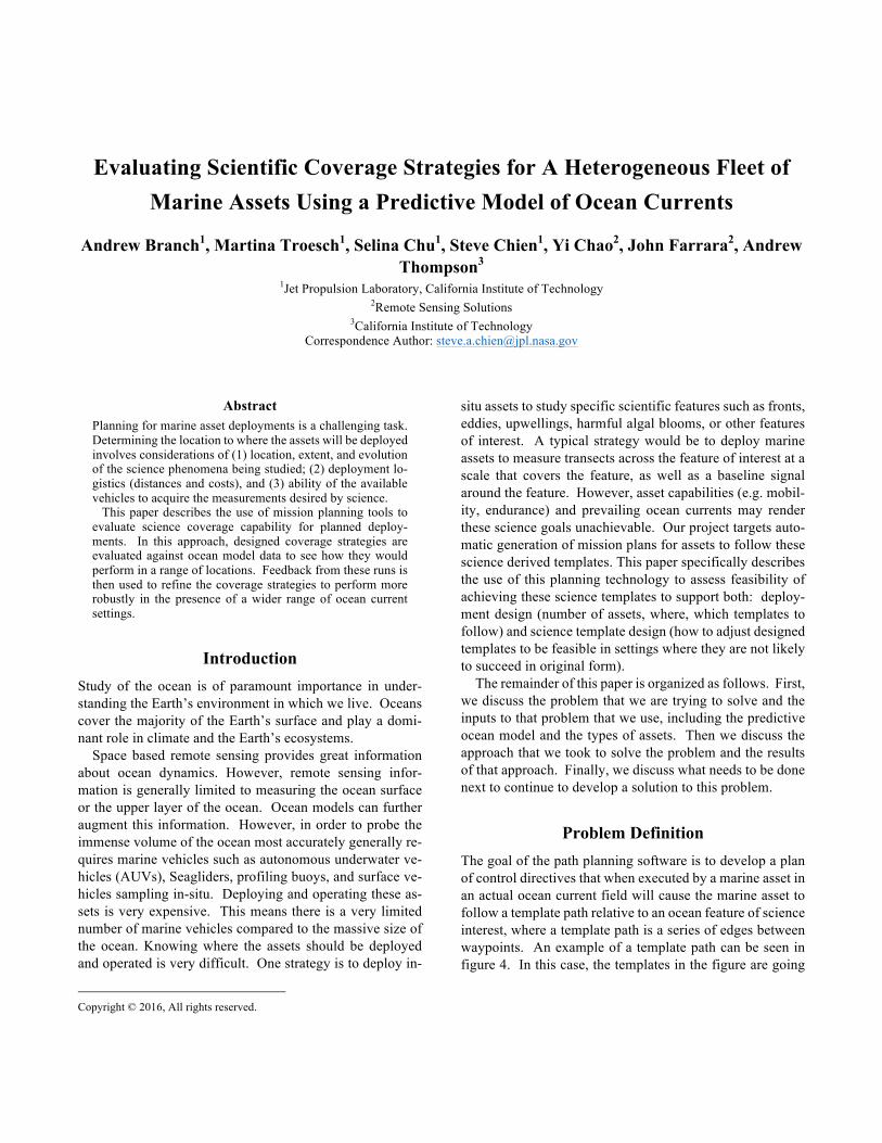
Beam Search The beam search next state generator can be seen in algo-rithm 3. This algorithm limits the number of possible next states to N bearings that are selected over some search angle theta. This search angle is centered on the bearing that points to the next template waypoint. For example, with a beam size of 5 and a search angle size of 30 degrees centered at 0 degrees, the bearings used to determine the next states would be -15, -7.5, 0, 7.5, and 15 degrees. The command point that is selected for each next state is set at a distance from the assets current location equal to the distance that as-set would travel before the next time that it could be com-manded, or the distance to the next waypoint on the template path, whichever is closer. Figure 2 shows the next states

Figure 1: Graph of Seaglider and AUV movement with surface activities labelled.

Algorithm 3: Beam Search Next State Note: Uses Planning Model function BeamSearchNextState(node, templatePath) curWaypoint ← next waypoint in templatePath bearing ← bearing from node to curWaypoint curBearing ← bearing – search angle while curBearing < bearing + search angle do if distance to curWaypoint > command time * speed then point ← distance to curWaypoint at curBearing else point ← command time * speed at curBearing newNode ← simulate movement from current loca-tion to point newNode.planningPoints add point neighbors ← neighbors + newNode curBearing += search angle / (branching factor – 1) return neighbors end function

produced by beam search. The green arc is the valid angle that the bearings are chosen from, notice that it is centered on the bearing from the asset to the next template waypoint. N bearings are selected uniformly over this arc. In the case of the figure, N is 3. Note that this is different from a stand-ard beam search. Normally every possible next state would be judged by a heuristic, then the top N would be used (Rus-sell and Norvig 2009). In this case we calculate a fixed delta angle between the bearings as follows

∆𝑎𝑛𝑔𝑙𝑒 =𝑎

(𝑛 − 1)

where a is the size of the search angle and n is the beam size. This is similar to using the top scoring heuristic with no cur-rents, as the optimal bearing would be directly toward the next template waypoint. The beam search approach has the benefit of using the predictive ocean model currents to better predict the trajec-tory that an asset will take. When the planning model is ac-curate then this helps to keep the asset on course and arrive at the next template waypoint more quickly and reliably. However, when the planning model is not accurate this ap-proach can actually make the situation worse. The approach was chosen as a way to discretize the pos-sible command points that the asset could be commanded with. The set of possible bearings is limited to some search angle toward the next waypoint as it is very unlikely that the optimal direction of travel is going to be significantly differ-ent from the direction that the waypoint is in. The search angle is then discretized into N bearings as a small different in the angle is unlikely to have a large effect on the end re-sult. This discretization greatly simplifies the search process by taking it out of the continuous space.

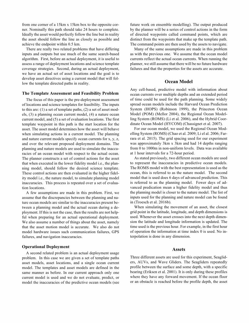
Algorithms For this experiment, a continuous planner is used. A graph-ical representation of this algorithm is shown in figure 3. This algorithm runs a best-first search, using the planning model, starting from the assets current location, and with a template path that contains the waypoints that have not yet been visited. The best-first search algorithm generates a list of command points that are then given to continuous plan-ner. Note that these command points are distinct from those that make up the template path. The blue lines in the figure represent that path that the best-first search finds and the red points are the command points that the are returned to the

continuous planner. These points are used to simulate the movement of the asset with the nature model. The bearing of the asset is set so that it is heading toward the next com-mand point. Every time the asset is able to update its loca-tion, this bearing is updated. How often the location can be updated depends on the asset being used. The asset is simulated for an amount of time equal to the time between re-commanding the asset, this also depends on the asset being used. If the command point is reached before this re-command time, then the next command point in the list is used. A command point is considered to be reached if the asset passes within a certain threshold distance from it. Each time an asset can be re-commanded the best-first search is run again, starting at the updated location of the asset. The old command points are discarded and the new ones from the best-first search are used until the next re-command. This process repeats until the goal is reached. In this case the goal state is successfully visiting every template waypoint in order. This process of repeated planning and simulation emulates the actual deployment of these assets. The best-first search also stores the best result seen so far. This is returned after a fixed number of iterations to prevent the search from attempting to exhaust every path when it is not possible to reach the goal state before the mission length has been exceeded, as this is impractical even for small

Figure 1: Graphic representation of the beam search next state generator. The

search angle is the green arc and the next command points are labelled.

Algorithm 1: Continuous Planner Note: Uses Nature Model for simulating movement function ContinuousPlanner(startLocation, template-Path)

curPath ← startLocation curWaypoint ← second waypoint on templatePath while true do endNode ← last node in curPath

planPoints ← BestFirstSearch(endNode, template-Path)

point ← first point in planPoints while time till re-command > 0 do newNode ← simulate movement to planPoint

curPath ← curPath + newNode if newNode distance to point <= threshold then point ← next point in planPoints

if newNode distance to curWaypoint <= threshold then

if curWaypoint is final waypoint in template-Path then

return success curWaypoint ← next waypoint on template

path if curPath duration > mission length then return failure

end function

branching factors. Increasing this threshold will improve the results at the cost of extended runtime.

Best-First Search

The objective function that was used for best-first search combines distance travelled and time taken. The equation is

𝑤. ∗𝑑1𝑑2+ 𝑤2 ∗

𝑡1𝑡2

where wd and wt are weighting factors for the distance and time portions of the equation respectively, dp is distance travelled thus far by the asset, dt is the total distance of the template path, tp is the total time taken by the asset so far, and tt is the target time to complete the template path. The larger the ratio of wd to wt the more the algorithm will favor shorter distance paths over shorter time paths. By reducing the distance travelled the resulting path will stay closer to the template path even though the average distance from the template path is not included in the calculation. The objective function takes into account the two metrics that we are using to evaluate the quality of the paths, time

and distance. As these two metrics have completely sepa-rate units the ratio of distance travelled to expected total dis-tance and the ratio of current time to target time are used instead. This allows them to be equated more easily. The heuristic function used by the best-first search is the following equation

𝑤2 ∗𝑑5𝑠7∗1𝑡2+ 𝑤. ∗

𝑑5𝑑2

where wd and wt are weighting factors for the distance and time portions of the equation respectively, sa is the horizon-tal speed of the asset, dl is distance left to travel, tt is the target time to complete to template path, and dt is the total distance of the template path. As the asset is further along in the template path this number will decrease. In practice, this heuristic is only a measure of the distance left to travel, as the time left has a linear relationship with the distance. The two terms are calculated separately so the heuristic is weighted appropriately with respect to the objective func-tion. An approach similar to the one used for the objective function is used for the heuristic function. The ratio of the estimated distance left to the total distance of the template path and the ratio of the estimated time left to the total target time is used.

Experiment Setup

Seaglider The Seagliders were given a speed of 0.266 m/s, a glide slope of 20 degrees, and a maximum depth of 500 meters. They were commanded every 3 hours. This is equivalent to one complete profile. At each surface from a profile the Sea-glider location is updated. This allows the asset to adjust its bearing to point toward the next command point it is travel-ling to. The template path was from one corner of a 15km x 15km box to the opposite corner. This was done for the two diagonal pairs in each direction, for a total of 4 runs per lo-cation. Each run has a target completion time of 24 hours. The template waypoints have a threshold distance of 0.5 km. This is the distance that the Seaglider can be from the way-point while still be considered to have visited it. During a deployment there would be two Seagliders operating con-currently, one for each diagonal. This pattern can been see in figure 4.

Figure 2: Graphic representation of the continuous planning process.

Algorithm 2: Best-First Search Note: Uses Planning Model function BestFirstSearch(startNode, templatePath)

Q ← startNode best ← startNode while Q not empty do curNode ← lowest score node in Q if best score < curNode score then best ← curNode if curNode is a goal state then return curNode.planningPoints if node expansion limit reached then return best.planningPoints neighbors ← next-state-generator(curNode, template-Path) for each neighbor in neighbors do Q ← neighbor

end function

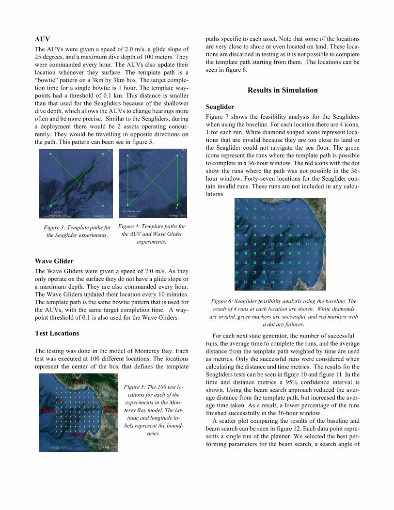
AUV The AUVs were given a speed of 2.0 m/s, a glide slope of 25 degrees, and a maximum dive depth of 100 meters. They were commanded every hour. The AUVs also update their location whenever they surface. The template path is a “bowtie” pattern on a 3km by 3km box. The target comple-tion time for a single bowtie is 1 hour. The template way-points had a threshold of 0.1 km. This distance is smaller than that used for the Seagliders because of the shallower dive depth, which allows the AUVs to change bearings more often and be more precise. Similar to the Seagliders, during a deployment there would be 2 assets operating concur-rently. They would be travelling in opposite directions on the path. This pattern can been see in figure 5.

Wave Glider The Wave Gliders were given a speed of 2.0 m/s. As they only operate on the surface they do not have a glide slope or a maximum depth. They are also commanded every hour. The Wave Gliders updated their location every 10 minutes. The template path is the same bowtie pattern that is used for the AUVs, with the same target completion time. A way-point threshold of 0.1 is also used for the Wave Gliders.

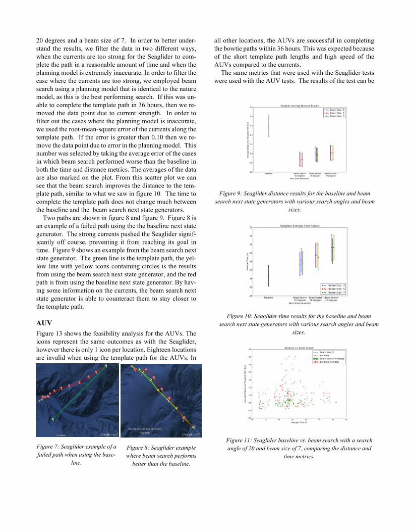
Test Locations The testing was done in the model of Monterey Bay. Each test was executed at 100 different locations. The locations represent the center of the box that defines the template

paths specific to each asset. Note that some of the locations are very close to shore or even located on land. These loca-tions are discarded in testing as it is not possible to complete the template path starting from them. The locations can be seen in figure 6.

Results in Simulation

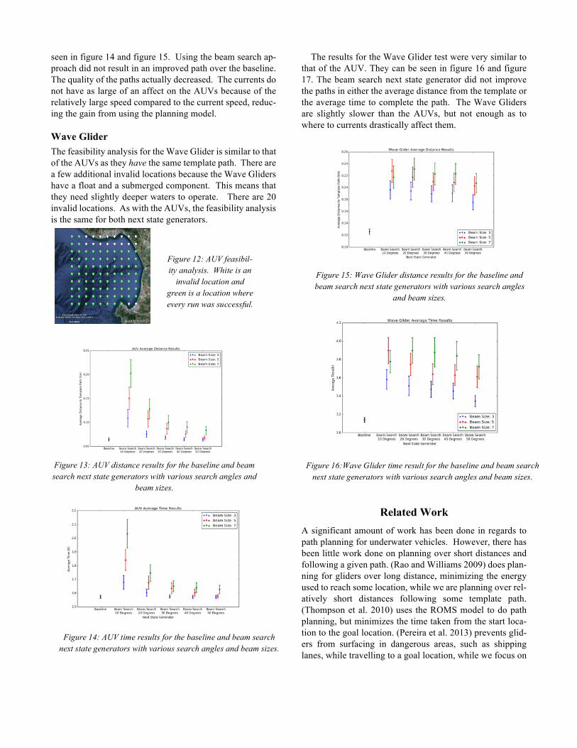
Seaglider Figure 7 shows the feasibility analysis for the Seagliders when using the baseline. For each location there are 4 icons, 1 for each run. White diamond shaped icons represent loca-tions that are invalid because they are too close to land or the Seaglider could not navigate the sea floor. The green icons represent the runs where the template path is possible to complete in a 36-hour window. The red icons with the dot show the runs where the path was not possible in the 36-hour window. Forty-seven locations for the Seaglider con-tain invalid runs. These runs are not included in any calcu-lations.

For each next state generator, the number of successful runs, the average time to complete the runs, and the average distance from the template path weighted by time are used as metrics. Only the successful runs were considered when calculating the distance and time metrics. The results for the Seagliders tests can be seen in figure 10 and figure 11. In the time and distance metrics a 95% confidence interval is shown. Using the beam search approach reduced the aver-age distance from the template path, but increased the aver-age time taken. As a result, a lower percentage of the runs finished successfully in the 36-hour window. A scatter plot comparing the results of the baseline and beam search can be seen in figure 12. Each data point repre-sents a single run of the planner. We selected the best per-forming parameters for the beam search, a search angle of

Figure 3: Template paths for the Seaglider experiments.

Figure 4: Template paths for the AUV and Wave Glider

experiments.

Figure 5: The 100 test lo-cations for each of the

experiments in the Mon-terey Bay model. The lat-itude and longitude la-

bels represent the bound-aries.

Figure 6: Seaglider feasibility analysis using the baseline. The result of 4 runs at each location are shown. White diamonds

are invalid, green markers are successful, and red markers with a dot are failures.

20 degrees and a beam size of 7. In order to better under-stand the results, we filter the data in two different ways, when the currents are too strong for the Seaglider to com-plete the path in a reasonable amount of time and when the planning model is extremely inaccurate. In order to filter the case where the currents are too strong, we employed beam search using a planning model that is identical to the nature model, as this is the best performing search. If this was un-able to complete the template path in 36 hours, then we re-moved the data point due to current strength. In order to filter out the cases where the planning model is inaccurate, we used the root-mean-square error of the currents along the template path. If the error is greater than 0.10 then we re-move the data point due to error in the planning model. This number was selected by taking the average error of the cases in which beam search performed worse than the baseline in both the time and distance metrics. The averages of the data are also marked on the plot. From this scatter plot we can see that the beam search improves the distance to the tem-plate path, similar to what we saw in figure 10. The time to complete the template path does not change much between the baseline and the beam search next state generators. Two paths are shown in figure 8 and figure 9. Figure 8 is an example of a failed path using the the baseline next state generator. The strong currents pushed the Seaglider signif-icantly off course, preventing it from reaching its goal in time. Figure 9 shows an example from the beam search next state generator. The green line is the template path, the yel-low line with yellow icons containing circles is the results from using the beam search next state generator, and the red path is from using the baseline next state generator. By hav-ing some information on the currents, the beam search next state generator is able to counteract them to stay closer to the template path.

AUV Figure 13 shows the feasibility analysis for the AUVs. The icons represent the same outcomes as with the Seaglider, however there is only 1 icon per location. Eighteen locations are invalid when using the template path for the AUVs. In

all other locations, the AUVs are successful in completing the bowtie paths within 36 hours. This was expected because of the short template path lengths and high speed of the AUVs compared to the currents. The same metrics that were used with the Seaglider tests were used with the AUV tests. The results of the test can be

Figure 9: Seaglider distance results for the baseline and beam search next state generators with various search angles and beam

sizes.

Figure 10: Seaglider time results for the baseline and beam search next state generators with various search angles and beam

sizes.

Figure 11: Seaglider baseline vs. beam search with a search angle of 20 and beam size of 7, comparing the distance and

time metrics. Figure 7: Seaglider example of a failed path when using the base-

line.

Figure 8: Seaglider example where beam search performs

better than the baseline.

seen in figure 14 and figure 15. Using the beam search ap-proach did not result in an improved path over the baseline. The quality of the paths actually decreased. The currents do not have as large of an affect on the AUVs because of the relatively large speed compared to the current speed, reduc-ing the gain from using the planning model.

Wave Glider The feasibility analysis for the Wave Glider is similar to that of the AUVs as they have the same template path. There are a few additional invalid locations because the Wave Gliders have a float and a submerged component. This means that they need slightly deeper waters to operate. There are 20 invalid locations. As with the AUVs, the feasibility analysis is the same for both next state generators.

The results for the Wave Glider test were very similar to that of the AUV. They can be seen in figure 16 and figure 17. The beam search next state generator did not improve the paths in either the average distance from the template or the average time to complete the path. The Wave Gliders are slightly slower than the AUVs, but not enough as to where to currents drastically affect them.

Related Work A significant amount of work has been done in regards to path planning for underwater vehicles. However, there has been little work done on planning over short distances and following a given path. (Rao and Williams 2009) does plan-ning for gliders over long distance, minimizing the energy used to reach some location, while we are planning over rel-atively short distances following some template path. (Thompson et al. 2010) uses the ROMS model to do path planning, but minimizes the time taken from the start loca-tion to the goal location. (Pereira et al. 2013) prevents glid-ers from surfacing in dangerous areas, such as shipping lanes, while travelling to a goal location, while we focus on

Figure 12: AUV feasibil-ity analysis. White is an

invalid location and green is a location where every run was successful.

Figure 13: AUV distance results for the baseline and beam search next state generators with various search angles and

beam sizes.

Figure 14: AUV time results for the baseline and beam search next state generators with various search angles and beam sizes.

Figure 15: Wave Glider distance results for the baseline and beam search next state generators with various search angles

and beam sizes.

Figure 16:Wave Glider time result for the baseline and beam search next state generators with various search angles and beam sizes.

following a specific path. (Cashmore et al. 2014) uses AUVs to inspect features at a site efficiently. No ocean model sim-ilar to ROMS was used. (Alvarez, Garau, and Caiti 2007) also does not use an ocean model, but instead uses synthetic data with general algorithms to control a set of floats and gliders. (Dahl et al. 2011) and (Troesch et al. 2016a, Troesch et al. 2016b) address the control of vertically pro-filing floats using a current model but do not address other types of marine vehicles. Continuous planning has become more prevalent in re-cent years and the evolution of this planning technique, with respect to multiple assets, is clearly described in (Durfee et al. 1999). (Myers 1999) describes a Continuous Planning and Execution Framework (CPEF), which integrates plan-ning and execution through plan generation, monitoring, ex-ecution, and repair. Using an iterative repair process, as well as user interaction, CPEF is able to plan in unpredictable and dynamic environments, which is shown through tests in a simulation of an air-campaign for dominance. (Chien et al. 2000) presents Continuous Activity Scheduling Planning Execution and Replanning (CASPER), which also uses iter-ative repair as part of continuous planning, specifically for autonomous spacecraft control.

Future Work There are a number of different possible extensions to this experiment. Different next state generators and heuristics could be developed that focus on the assets that did not ben-efit from the approach in this work. More research into the performance characteristics of beam search and the associ-ated heuristics could be done. The beam search next state generator could be improved to select the next states more intelligently. Tests could be performed in different areas, such as those with stronger currents and different template paths could be used to better understand the behavior of the planner. The drop off location of the asset could be included in the planning. Ocean models with different fidelity could be used to understand the performance of the planner with more or less accurate models. A range of methods for inter-polating the current model information between data points could be explored. Additionally, ROMS provides ensemble information from multiple runs with varying conditions, the planner could use search in the ensemble space and/or use ensembles to predict execution uncertainty and incorporate this to inform the generation process. Multi-agent planning could be used for multiple assets to achieve a goal. The us-age of the model could be improved to include interpolation between the grid points.

Conclusion This experiment has shown the benefits of using a predictive ocean model to do planning in order for an underwater ve-hicle to follow a template path. With the Seaglider, the beam search next state generator improved how well the as-set could follow the template path compared to the baseline. However, with this result came a slight increase on the time taken to complete the template path. However, this benefit does not extend to every type of as-set. The baseline performed better than beam search when using Wave Gliders and AUVs in both how well the tem-plate path was followed and the time to complete the path. It is clear that the amount of benefit from this approach de-pends heavily on the vehicle and path in question. As such, a single approach may not be applicable to a wide variety of assets. More research needs to be done in order to fully under-stand the behavior of the beam search next state generator and the associated objective and heuristic functions.

Acknowledgements Portions of this work were performed at the Jet Propulsion Laboratory, California Institute of Technology, under con- tract with the National Aeronautics and Space Administra- tion.

References Alvarez, A.; Garau, B.; and Caiti, A. 2007. Combining networks of drifting profiling floats and gliders for adaptive sampling of the ocean. In Robotics and Automation, 2007 IEEE International Con-ference on, 157–162. IEEE. Cashmore, M.; Fox, M.; Larkworthy, T.; Long, D.; and Mag- azzeni, D. 2014. Auv mission control via temporal planning. In Ro-botics and Automation (ICRA), 2014 IEEE International Confer-ence on, 6535–6541. IEEE. Chao, Y.; Li, Z.; Farrara, J.; McWilliams, J. C.; Bellingham, J.; Capet, X.; Chavez, F.; Choi, J.-K.; Davis, R.; Doyle, J.; et al. 2009. Development, implementation and evaluation of a data-assimila-tive ocean forecasting system off the central california coast. Deep Sea Research Part II: Topical Studies in Oceanography 56(3):100–126. Chassignet, E. P.; Hurlburt, H. E.; Smedstad, O. M.; Halliwell, G. R.; Hogan, P. J.; Wallcraft, A. J.; Baraille, R.; and Bleck, R. 2007. The hycom (hybrid coordinate ocean model) data assimilative sys-tem. Journal of Marine Systems 65(1):60–83. Chien, S. A.; Knight, R.; Stechert, A.; Sherwood, R.; and Rabideau, G. 2000. Using iterative repair to improve the respon-siveness of planning and scheduling. In AIPS, 300– 307. Dahl, K. P.; Thompson, D. R.; McLaren, D.; Chao, Y.; and Chien, S. 2011. Current-sensitive path planning for an un- deractuated free-floating ocean sensorweb. In Intelligent Robots and Systems (IROS), 2011 IEEE/RSJ International Conference on, 3140–3146. IEEE.

Durfee, E. H.; Ortiz Jr, C. L.; Wolverton, M. J.; et al. 1999. A sur-vey of research in distributed, continual planning. Ai magazine 20(4):13–22. Eriksen, C. C.; Osse, T. J.; Light, R. D.; Wen, T.; Lehman, T. W.; Sabin, P. L.; Ballard, J. W.; and Chiodi, A. M. 2001. Seaglider: A long-range autonomous underwater vehicle for oceanographic re-search. Oceanic Engineering, IEEE Journal of 26(4):424–436. Farrara, J. D.; Chao, Y.; Zhang, H.; Seegers, B. N.; Teel, E. N.; Caron, D. A.; Howard, M.; Jones, B. H.; Robertson, G.; Rogowski, P.; and Terrill, E. 2015. Oceanographic conditions during the or-ange county sanitation district diversion experiment as revealed by observations and model simulations. Submitted to Estuarine, Coastal and Shelf Science. Li, P.; Chao, Y.; Vu, Q.; Li, Z.; Farrara, J.; Zhang, H.; and Wang, X. 2006. Ourocean-an integrated solution to ocean monitoring and forecasting. In OCEANS 2006, 1–6. IEEE. Manley J. 2010. The Wave Glider: A persistent platform for ocean science. In OCEANS 2010, 1-5. IEEE-Sydney. Mellor, G. L. 2004. Users guide for a three dimensional, primitive equation, numerical ocean model. Princeton, NJ: Princeton Uni-versity. Myers, K. L. 1999. Cpef: A continuous planning and exe- cution framework. AI Magazine 20(4):63–69. Pereira, A. A.; Binney, J.; Hollinger, G. A.; and Sukhatme, G. S. 2013. Risk-aware path planning for autonomous underwater vehi-cles using predictive ocean models. Journal of Field Robotics 30(5):741–762. Rao, D., and Williams, S. B. 2009. Large-scale path planning for underwater gliders in ocean currents. In Australasian Conference on Robotics and Automation (ACRA), Sydney. Citeseer. Robinson, A. R. 1999. Forecasting and simulating coastal ocean processes and variabilities with the Harvard Ocean Prediction Sys-tem. In Mooers, C. N. K., ed., Coastal Ocean Prediction, AGU Coastal and Estuarine Studies Se- ries. Washington, DC: American Geophysical Union. 77– 100. Russell S.; Norvig P. Artificial Intelligence: A Modern Approach (Third Edition), Prentice Hall, 2009 Thompson, D. R.; Chien, S.; Chao, Y.; Li, P.; Cahill, B.; Levin, J.; Schofield, O.; Balasuriya, A.; Petillo, S.; Arrott, M.; et al. 2010. Spatiotemporal path planning in strong, dynamic, uncertain cur-rents. In Robotics and Automation (ICRA), 2010 IEEE Interna-tional Conference on, 4778– 4783. IEEE. Troesch M.; Chien S.; Chao Y.; and Farrara J. 2016 Planning and control of marine floats in the presence of dynamic, uncertain cur-rents . International Conference on Automated Planning and Scheduling (ICAPS) 2016. Troesch M.; Chien S.; Chao Y.; and Farrara J. 2016 Evaluating the Impact of Model Accuracy in Batch and Continuous Planning for Control of Marine Floats. Scheduling and Planning Applications Workshop, International Conference on Automated Planning and Scheduling (ICAPS) 2016. (under review) YSI Systems. “EcoMapper AUV”. http://www.ysisystems.com. Accessed February, 2016.