Evaluating the Double Poisson Generalized Linear Model · PDF fileEvaluating the Double Poisson Generalized Linear Model Yaotian Zou1 Research Assistant ... The hurdle of applying

Evaluating the Double Poisson Generalized Linear Model

Yaotian Zou1 Research Assistant

School of Civil Engineering Purdue University

550 Stadium Mall Drive West Lafayette, IN 47907-2051

Email: [email protected]

Srinivas Reddy Geedipally2 Assistant Research Engineer

Texas Transportation Institute Texas A&M University System

110 N. Davis Dr. 101 Arlington, TX 76013 Tel. (817) 462-0519


Dominique Lord Associate Professor and Zachry Development Professor I

Zachry Department of Civil Engineering Texas A&M University, 3136 TAMU

College Station, TX 77843-3136 Tel. (979) 458-3949


July 15, 2013

1The work was done while the author was in Texas A&M University 2Corresponding author

ABSTRACT The objectives of this study are to: 1) examine the applicability of the double Poisson (DP) generalized linear model (GLM) for analyzing motor vehicle crash data characterized by over- and under-dispersion and 2) compare the performance of the DP GLM with the Conway-Maxwell-Poisson (COM-Poisson) GLM in terms of goodness-of-fit and theoretical soundness. The DP distribution has seldom been investigated and applied since its first introduction two decades ago. The hurdle of applying the DP is related to its normalizing constant (or multiplicative constant) which is not available in closed form. This study proposed a new method to approximate the normalizing constant of the DP with high accuracy and reliability. The DP GLM and COM-Poisson GLM were developed using two observed over-dispersed datasets and one observed under-dispersed dataset. The modeling results indicate that the DP GLM with its normalizing constant approximated by the new method can handle crash data characterized by over- and under-dispersion. Its performance is comparable to the COM-Poisson GLM in terms of goodness-of-fit (GOF), although COM-Poisson GLM provides a slightly better fit. For the over-dispersed data, the DP GLM performs similar to the NB GLM. Considering the fact that the DP GLM can be easily estimated with inexpensive computation and that it is simpler to interpret coefficients, it offers a flexible and efficient alternative for researchers to model the count data.

Zou, Geedipally and Lord 1

1. INTRODUCTION Due to the limited access to driving information, it is very difficult to identify factors (e.g., brake reaction time, inattention, etc.) directly influencing the number and severity of motor vehicle crashes in traffic safety analysis. Thus, instead of focusing on individual driver’s information, most researchers approach crash causal or correlation analyses from a long term statistical view. In this regards, researchers try to associate the factors of interest with the frequency of crashes that occurs in a given space (roadway or intersection) and time period (Lord and Mannering, 2010). Therefore, statistical models have been the analysis tool of choice for analyzing the relationship between motor vehicle crashes and factors such as road section geometric design, traffic flow, weather, etc.

The traditional Poisson has been commonly used to model motor vehicle crashes. Despite its simple probabilistic structure, the traditional Poisson distribution has a strict assumption in that its single parameter does not allow for the flexibility of variance varying independently of the mean, which is often violated by its application to the over-dispersed (i.e., the sample variance is larger than the sample mean) and under-dispersed (i.e., the sample variance is smaller than the sample mean) crash data. Under-dispersion occurs on rare occasions and this often happens when the sample mean value is low (Lord and Mannering, 2010). Over-dispersed and under-dispersed data can lead to inconsistent standard errors of parameter estimates when the Poisson model is used (Cameron and Trivedi, 1998; Park and Lord, 2007).

Over the last three decades, the negative binomial distribution or model (NB or Poisson-gamma) has been quite popular to handle the over-dispersed datasets. Although the mean-variance relationship of the NB is simple to manipulate so as to capture over-dispersion (Hauer, 1997), it has been found to have difficulties in handling the data characterized by under-dispersion (Lord et al., 2008a). Though crash data do not exhibit under-dispersion very often, it is observed more frequently in other fields of research (for example, see Guikema and Coffelt, 2008; Sellers and Shmueli, 2010; Borle et al., 2006). In order to manage data characterized by over-dispersion and under-dispersion, researchers have proposed alternative models such as the weighed Poisson distribution (Castillo and Perez-Casany, 2005), the generalized Poisson distribution (Consul, 1989) and the gamma count distribution (Winkelmann, 2008). However, these models suffered from important theoretical or logical soundness. For instance, the weighted Poisson distribution has convergence restrictions and it is necessary to choose an appropriate function, which is sometimes difficult to do. With the generalized Poisson model, the bounded dispersion parameter when under-dispersion occurs greatly diminishes its applicability to count data (Famoye, 1993) and the model does not include the Poisson family in the interior of the parameter space (Castillo and Perez-Casany, 2005). The gamma count distribution assumes that observations are not independent where the observation for time t-1 would affect the observation for time t (Winkelmann, 2008; Cameron and Trivedi, 1998). This would become unrealistic if the time gap between the two observations is large, which can be problematic for analyzing crash data.

Among the distributions or models that have been documented in the literature, two distributions that can handle both under- and over-dispersion are particularly noteworthy. One is the Conway-Maxwell-Poisson (COM-Poisson or CMP) distribution (Conway and Maxwell, 1962; Shmueli et al., 2005; Kadane et al., 2006) and the other is the double Poisson (DP) distribution (Efron, 1986). Albeit first introduced in 1962, the statistical properties of the COM-Poisson have not been extensively investigated until recently. The COM-Poisson distribution and its generalized linear model (GLM) have been found to be very flexible to handle count data


(Guikema and Coffelt, 2008; Lord et al., 2008a; Sellers et al., 2012; Francis et al., 2012). As for the DP, its distribution has seldom been investigated and applied since its first introduction about 25 years ago. A handful of research studies have mentioned that the hurdle of applying the DP is its normalizing constant (or multiplicative constant), which is not available in the closed form (Winkelmann, 2008; Hilbe, 2011; Zhu, 2012). They found that the results of the DP with its normalizing constant approximated by Efron’s original method are not exact. Instead of using Efron’s approximation method, this study documents a different method for handling the normalizing constant.

The objectives of this study are to: 1) examine the applicability of the DP GLM for analyzing motor vehicle crash data characterized by over- and under-dispersion and 2) compare the performance of the DP GLM with COM-Poisson GLM in terms of goodness-of-fit and theoretical soundness. Two empirical over-dispersed datasets (one for the high mean scenario and one for the low mean scenario) and one empirical under-dispersed dataset were used.

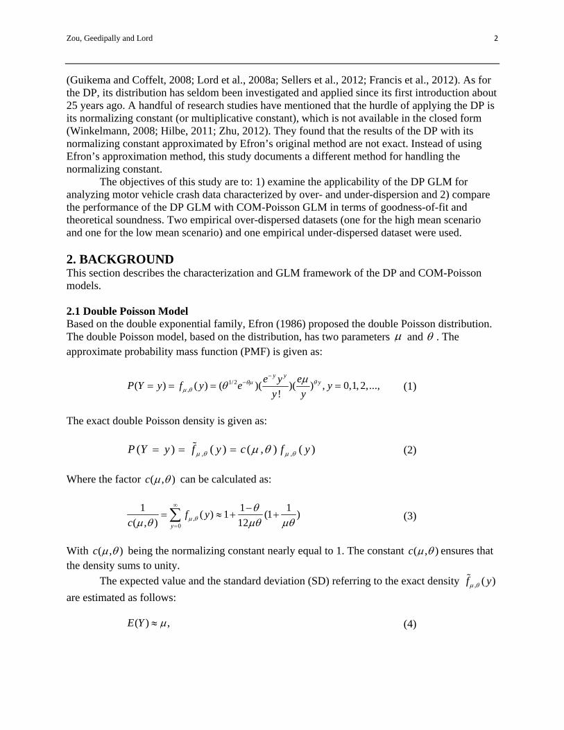
2. BACKGROUND This section describes the characterization and GLM framework of the DP and COM-Poisson models. 2.1 Double Poisson Model Based on the double exponential family, Efron (1986) proposed the double Poisson distribution. The double Poisson model, based on the distribution, has two parameters and . The approximate probability mass function (PMF) is given as:

1/2,( ) ( ) ( )( )( ) , 0,1, 2,...,

!

y yye y e

P Y y f y e yy y

(1)

The exact double Poisson density is given as:

, ,( ) ( ) ( , ) ( )P Y y f y c f y (2)

Where the factor ( , )c can be calculated as:

,0

1 1 1( ) 1 (1 )

( , ) 12y

f yc

(3)

With ( , )c being the normalizing constant nearly equal to 1. The constant ( , )c ensures that the density sums to unity.

The expected value and the standard deviation (SD) referring to the exact density , ( )f y

are estimated as follows:

( ) ,E Y (4)


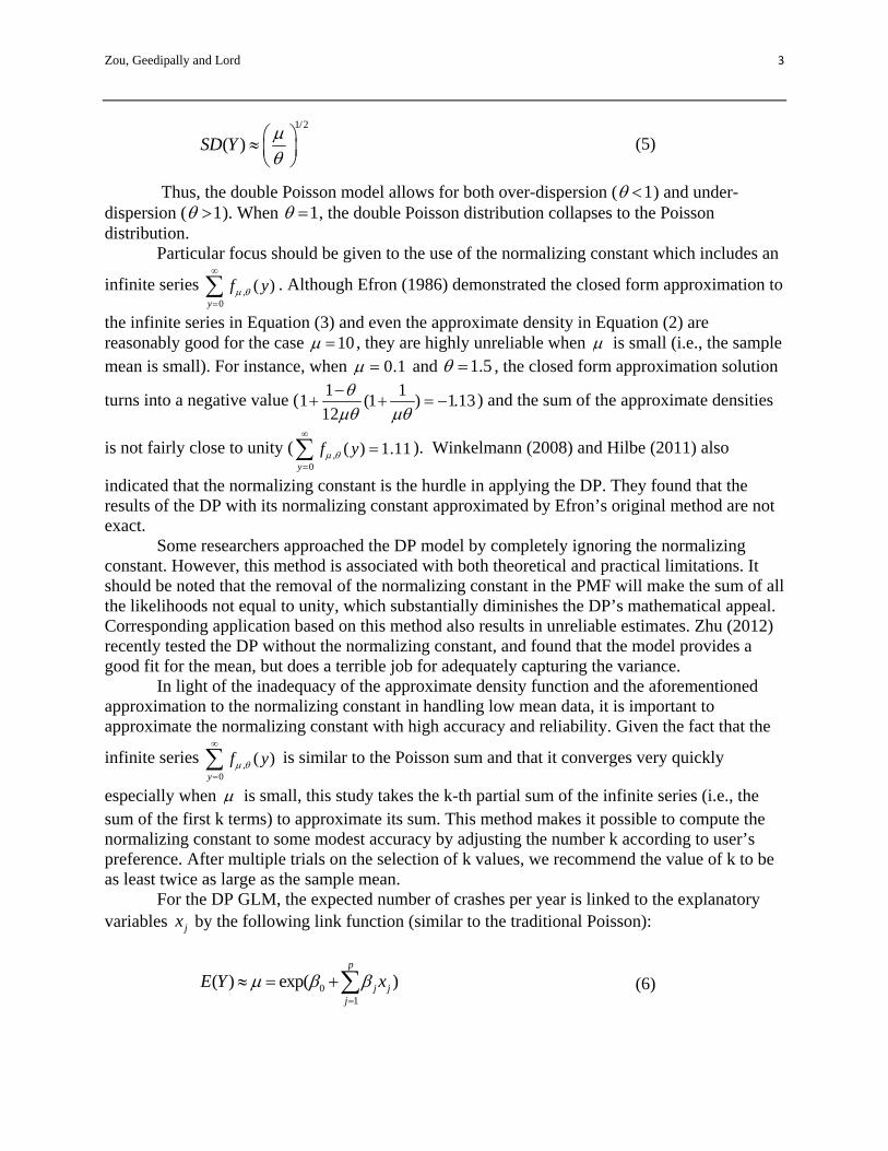
1/2

( )SD Y

(5)

Thus, the double Poisson model allows for both over-dispersion ( 1 ) and under-dispersion ( 1 ). When 1 , the double Poisson distribution collapses to the Poisson distribution. Particular focus should be given to the use of the normalizing constant which includes an

infinite series ,0

( )y

f y

. Although Efron (1986) demonstrated the closed form approximation to

the infinite series in Equation (3) and even the approximate density in Equation (2) are reasonably good for the case 10 , they are highly unreliable when is small (i.e., the sample mean is small). For instance, when 0.1 and 1.5 , the closed form approximation solution

turns into a negative value (1 1

1 (1 ) 1.1312

) and the sum of the approximate densities

is not fairly close to unity ( ,0

( ) 1.11y

f y

). Winkelmann (2008) and Hilbe (2011) also

indicated that the normalizing constant is the hurdle in applying the DP. They found that the results of the DP with its normalizing constant approximated by Efron’s original method are not exact. Some researchers approached the DP model by completely ignoring the normalizing constant. However, this method is associated with both theoretical and practical limitations. It should be noted that the removal of the normalizing constant in the PMF will make the sum of all the likelihoods not equal to unity, which substantially diminishes the DP’s mathematical appeal. Corresponding application based on this method also results in unreliable estimates. Zhu (2012) recently tested the DP without the normalizing constant, and found that the model provides a good fit for the mean, but does a terrible job for adequately capturing the variance.

In light of the inadequacy of the approximate density function and the aforementioned approximation to the normalizing constant in handling low mean data, it is important to approximate the normalizing constant with high accuracy and reliability. Given the fact that the

infinite series ,0

( )y

f y

is similar to the Poisson sum and that it converges very quickly

especially when is small, this study takes the k-th partial sum of the infinite series (i.e., the sum of the first k terms) to approximate its sum. This method makes it possible to compute the normalizing constant to some modest accuracy by adjusting the number k according to user’s preference. After multiple trials on the selection of k values, we recommend the value of k to be as least twice as large as the sample mean.

For the DP GLM, the expected number of crashes per year is linked to the explanatory variables jx by the following link function (similar to the traditional Poisson):

01

( ) exp( )p

j jj

E Y x

(6)


where the vector j is the coefficients to be estimated.

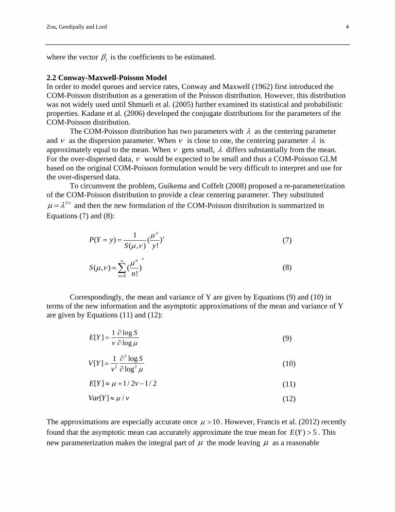
2.2 Conway-Maxwell-Poisson Model In order to model queues and service rates, Conway and Maxwell (1962) first introduced the COM-Poisson distribution as a generation of the Poisson distribution. However, this distribution was not widely used until Shmueli et al. (2005) further examined its statistical and probabilistic properties. Kadane et al. (2006) developed the conjugate distributions for the parameters of the COM-Poisson distribution.

The COM-Poisson distribution has two parameters with as the centering parameter and as the dispersion parameter. When is close to one, the centering parameter is approximately equal to the mean. When gets small, differs substantially from the mean. For the over-dispersed data, would be expected to be small and thus a COM-Poisson GLM based on the original COM-Poisson formulation would be very difficult to interpret and use for the over-dispersed data.

To circumvent the problem, Guikema and Coffelt (2008) proposed a re-parameterization of the COM-Poisson distribution to provide a clear centering parameter. They substituted

1/v and then the new formulation of the COM-Poisson distribution is summarized in Equations (7) and (8):

1

( ) ( )( , ) !

yvP Y y

S y

(7)

0

( , ) ( )!

vn

n

Sn

(8)

Correspondingly, the mean and variance of Y are given by Equations (9) and (10) in

terms of the new information and the asymptotic approximations of the mean and variance of Y are given by Equations (11) and (12):

1 log

[ ]log

SE Y

v

(9)

2

2 2

1 log[ ]

log

SV Y

v

(10)

[ ] 1 / 2 1/ 2E Y v (11)

[ ] /Var Y v (12)

The approximations are especially accurate once 10 . However, Francis et al. (2012) recently found that the asymptotic mean can accurately approximate the true mean for ( ) 5E Y . This new parameterization makes the integral part of the mode leaving as a reasonable


centering parameter. The substitution allows to keep its role as a shape parameter. That is, 1 leads to over-dispersion and 1 to under-dispersion.

Based on the new parameterization, Guikema and Coffelt (2008) developed a COM-Poisson GLM framework to model discrete count data using Bayesian framework in WinBUGS (Spiegelhalter et al., 2003). Their modeling framework is a dual-link GLM in which both the mean and variance depend on the covariates. It should be noted that parameter estimation for the dual-link GLM is complex and difficult. To make all the models in this paper comparable, this paper used the single-link COM-Poisson GLM framework (Lord et al., 2008a). The link function is given as:

01

( )p

j jj

ln x

(13)

where jx are the explanatory variables (traffic and geometric variables) and j are the

coefficients to be estimated. With the derivation of the likelihood function of the COM-Poisson GLM by Sellers and

Shmueli (2010), the maximum likelihood estimation (MLE) of the parameters of a COM-Poisson GLM was greatly simplified when compared to the Bayesian estimating method. The MLE-based COM-Poisson GLM is available in R package (COMPoissonReg on CRAN). Note that the MLE-based COM-Poisson GLM was developed under the original parameterization and thus it is difficult to interpret the coefficients in terms of their impact on the mean. 3. METHODOLOGY This section describes the link functions and parameter estimation methods for different models as well as the goodness-of-fit (GOF) statistics for comparing different models. 3.1 Link Function 3.1.1 Toronto Data For the first over-dispersed dataset (Toronto data), the linear predictor for all the models are linked to their respective centering parameter i . Note i here always do not denote the

expectation of a variable (i.e. ( )iE Y ). For the COM-Poisson GLM, it is not directly linked to the

expected mean as is the case with the NB GLM and DP GLM. The link function for the DP GLM is given as:

1 2

0 _ _( )i i Maj i Min iE Y F F (14)

The link function for the NB GLM is given as:

1 2

0 _ _( )i Maj i Min iE Y F F (15)

The link function for the COM-Poisson GLM is given as:


1 20 _ _i Maj i Min iF F (16)

Where,

( )iE Y = the mean number of crashes per year for intersection i;

i = the estimated centering parameter for the DP GLM or COM-Poisson GLM for

intersection i;

_Maj iF = entering flow for the major approach (or AADT) for intersection i;

_Min iF = entering flow for the minor approach (or AADT) for intersection i;

0 1 2, , = coefficients.

Although the functional form may be affected by the omitted variable bias (Lord and Mannering, 2010), it is still adequate for the purpose of this exercise.

With the parameters ˆi and v , the mean response for the COM-Poisson GLM can be

obtained using the asymptotic approximations given in Equation (11) (Lord et al., 2008a). However, it should be noted that the approximation is accurate only when 10 . Given the fact

that the sample mean is below 10, 100,000 samples were simulated for estimating ˆi and v for

the COM-Poisson GLMs. Then, the mean of those samples was as the mean response. For other methods on obtaining fitted values, the reader is referred to Sellers and Shmueli (2010).

3.1.2 Texas Data Similar to the Toronto data, the link function for the DP GLM when fitting the second over-dispersed dataset (Texas data) is given as:

2 3 41 _0( ) i i iLW SW CURVE DEN

i i i iE Y L F e (17)

The link function for the NB GLM is given as:

2 3 41 _0( ) i i iLW SW CURVE DEN

i i iE Y L F e (18)

The link function for the COM-Poisson GLM is given as:

2 3 41 _0

i i iLW SW CURVE DENi i iL F e (19)

Where,

( )iE Y = the mean number of KAB crashes per year for segment i;

i = the estimated centering parameter for DP GLM or COM-Poisson GLM for segment i;

iL= length of the segment in miles for segment i;

iF = the traffic flow volume (or AADT) in veh/day for segment i;

iLW = lane width in ft for segment i;


iSW = total shoulder width (both sides) in ft for segment i;

_ iCURVE DEN = number of horizontal curves per mile located on the segment i.

0 1 2 3 4, , , , = coefficients.

3.1.3 Under-Dispersed Data For the under-dispersed data, the link function for fitting all the models are the same with previous studies using this dataset (Oh et al., 2006; Lord et al., 2010):

0 1 1n( )

ni i ii

l F x

i e

(20)

Where,

i = the estimated centering parameter;

iF = the average daily traffic (ADT) in veh/day for segment i;

ix = the estimated covariates such as average daily railway traffic, presence of commercial

area etc.

i = coefficients.

3.2 Parameter Estimation The parameters of the DP GLMs were estimated using the NLMIXED procedure in SAS (SAS, 2002)1. The default quasi-Newton algorithm was applied to obtain the estimated parameters along with their approximate standard errors.

For the COM-Poisson GLM, the coefficients were estimated using the Bayesian framework in WinBUGS (Spiegelhalter et al., 2003). More information on estimating the coefficients of the COM-Poisson GLMs using WinBUGS can be found in Lord et al. (2008a).

3.3 Goodness-of-fit Statistics The following GOF statistics were used to compare different models for both over- and under-dispersed data:

Akaike Information Criterion (AIC) AIC is a measure that is used to describe the tradeoff between accuracy and complexity of the model. The model with smaller AIC is preferred to others. AIC is defined as:

2 log 2AIC L p (21)

1 The NLMIXED procedure was designed to fit nonlinear mixed models, that is, models with nonlinear random and fixed effects. The statement PROC NLMIXED offers an interface for specifying and coding a user-defined conditional distribution. Besides, PROC NLMIXED provides a variety of optimization techniques to maximize an approximation to the likelihood. Although NLMIXED procedure was often intended for mixed effects model, it was used to fit models with only fixed effects in this study.


where L is the maximized value of the likelihood function for the estimated model, and p is the number of parameters in the statistical model. By penalizing models with a large number of parameters, the AIC attempts to select the model that best explains the data with a minimum of parameters. Lower the AIC, better the model.

Deviance Information Criterion (DIC) The DIC is a hierarchical modeling generalization of the AIC. The model with smaller DIC is preferred to others. DIC is defined as:

DDIC D p (22)

where 2D LogL is the posterior mean of the deviance of the unstandardized model

and L is the mean of the model log likelihood. ( )Dp D D y is the effective model

parameters and is the expectation of .

Mean Prediction Bias (MPB) The MPB is used to measure the magnitude and direction of the average model bias. MPB is calculated using the following equation (Oh et al., 2003):

1

1ˆ( )

n

i ii

MPB y yn

(23)

where n is the sample size, iy and iy are the predicted and observed crashes at site i

respectively. When the model over-predicts crashes, MPB is positive and when the model under-predicts crashes, MPB is negative.

Mean Absolute Deviance (MAD) The MAD is the average of the absolute deviations and it measures the average mis-prediction of the model. The model closest to 0 is considered to be the best. It is computed by the following equation (Oh et al., 2003):

1

1ˆ

n

i ii

MAD y yn

(24)

Mean Squared Predictive Error (MSPE)

The MSPE is often used to access the error associated with a validation or external data set. The model closest to 0 is considered to be the best. It can be calculated by the following equation (Oh et al., 2003):


2

1

1ˆ( )

n

i ii

MSPE y yn

(25)

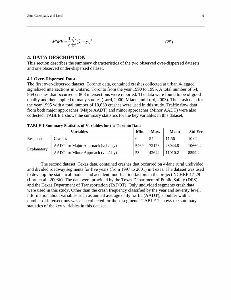
4. DATA DESCRIPTION This section describes the summary characteristics of the two observed over-dispersed datasets and one observed under-dispersed dataset. 4.1 Over-Dispersed Data The first over-dispersed dataset, Toronto data, contained crashes collected at urban 4-legged signalized intersections in Ontario, Toronto from the year 1990 to 1995. A total number of 54, 869 crashes that occurred at 868 intersections were reported. The data were found to be of good quality and then applied to many studies (Lord, 2000; Miaou and Lord, 2003). The crash data for the year 1995 with a total number of 10,030 crashes were used in this study. Traffic flow data from both major approaches (Major AADT) and minor approaches (Minor AADT) were also collected. TABLE 1 shows the summary statistics for the key variables in this dataset. TABLE 1 Summary Statistics of Variables for the Toronto Data

Variables Min. Max. Mean Std Err

Response Crashes 0 54 11.56 10.02

Explanatory AADT for Major Approach (veh/day) 5469 72178 28044.8 10660.4

AADT for Minor Approach (veh/day) 53 42644 11010.2 8599.4

The second dataset, Texas data, contained crashes that occurred on 4-lane rural undivided

and divided roadway segments for five years (from 1997 to 2001) in Texas. The dataset was used to develop the statistical models and accident modification factors in the project NCHRP 17-29 (Lord et al., 2008b). The data were provided by the Texas Department of Public Safety (DPS) and the Texas Department of Transportation (TxDOT). Only undivided segments crash data were used in this study. Other than the crash frequency classified by the year and severity level, information about variables such as annual average daily traffic (AADT), shoulder width, number of intersections was also collected for those segments. TABLE 2 shows the summary statistics of the key variables in this dataset.


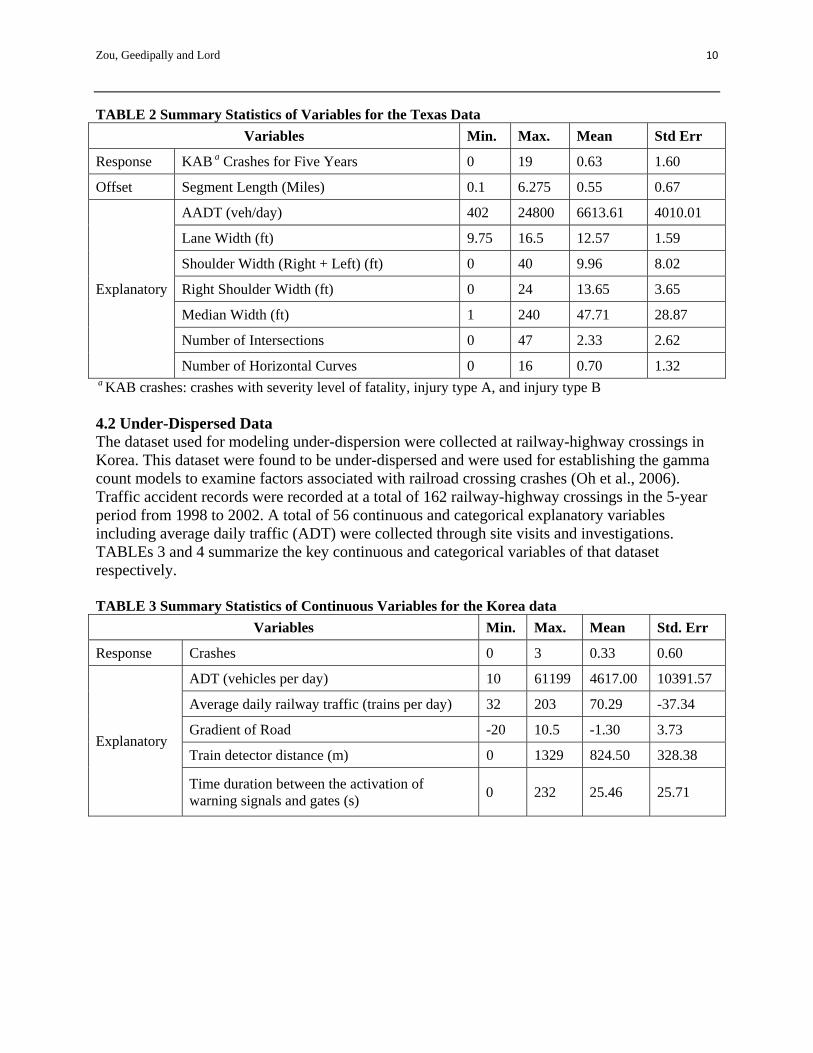
TABLE 2 Summary Statistics of Variables for the Texas Data

Variables Min. Max. Mean Std Err

Response KAB a Crashes for Five Years 0 19 0.63 1.60

Offset Segment Length (Miles) 0.1 6.275 0.55 0.67

Explanatory

AADT (veh/day) 402 24800 6613.61 4010.01

Lane Width (ft) 9.75 16.5 12.57 1.59

Shoulder Width (Right + Left) (ft) 0 40 9.96 8.02

Right Shoulder Width (ft) 0 24 13.65 3.65

Median Width (ft) 1 240 47.71 28.87

Number of Intersections 0 47 2.33 2.62

Number of Horizontal Curves 0 16 0.70 1.32 a KAB crashes: crashes with severity level of fatality, injury type A, and injury type B 4.2 Under-Dispersed Data The dataset used for modeling under-dispersion were collected at railway-highway crossings in Korea. This dataset were found to be under-dispersed and were used for establishing the gamma count models to examine factors associated with railroad crossing crashes (Oh et al., 2006). Traffic accident records were recorded at a total of 162 railway-highway crossings in the 5-year period from 1998 to 2002. A total of 56 continuous and categorical explanatory variables including average daily traffic (ADT) were collected through site visits and investigations. TABLEs 3 and 4 summarize the key continuous and categorical variables of that dataset respectively. TABLE 3 Summary Statistics of Continuous Variables for the Korea data

Variables Min. Max. Mean Std. Err

Response Crashes 0 3 0.33 0.60

Explanatory

ADT (vehicles per day) 10 61199 4617.00 10391.57

Average daily railway traffic (trains per day) 32 203 70.29 -37.34

Gradient of Road -20 10.5 -1.30 3.73

Train detector distance (m) 0 1329 824.50 328.38

Time duration between the activation of warning signals and gates (s)

0 232 25.46 25.71


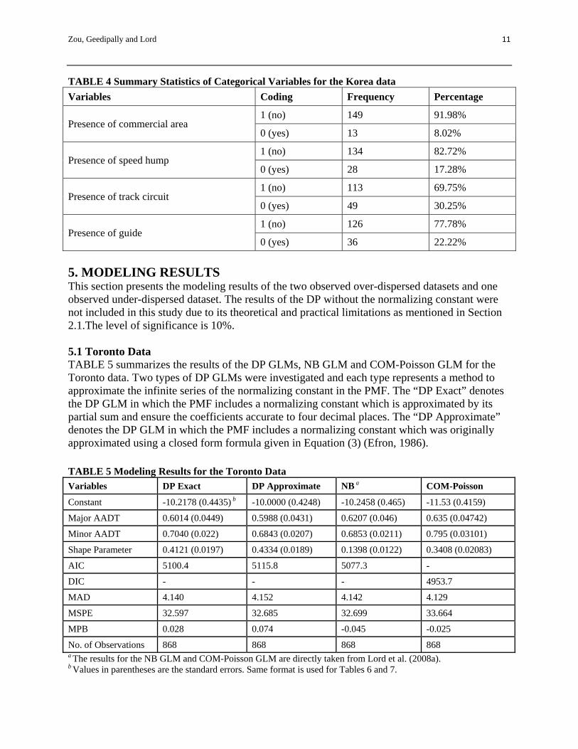
TABLE 4 Summary Statistics of Categorical Variables for the Korea data

Variables Coding Frequency Percentage

Presence of commercial area 1 (no) 149 91.98%

0 (yes) 13 8.02%

Presence of speed hump 1 (no) 134 82.72%

0 (yes) 28 17.28%

Presence of track circuit 1 (no) 113 69.75%

0 (yes) 49 30.25%

Presence of guide 1 (no) 126 77.78%

0 (yes) 36 22.22%

5. MODELING RESULTS This section presents the modeling results of the two observed over-dispersed datasets and one observed under-dispersed dataset. The results of the DP without the normalizing constant were not included in this study due to its theoretical and practical limitations as mentioned in Section 2.1.The level of significance is 10%. 5.1 Toronto Data TABLE 5 summarizes the results of the DP GLMs, NB GLM and COM-Poisson GLM for the Toronto data. Two types of DP GLMs were investigated and each type represents a method to approximate the infinite series of the normalizing constant in the PMF. The “DP Exact” denotes the DP GLM in which the PMF includes a normalizing constant which is approximated by its partial sum and ensure the coefficients accurate to four decimal places. The “DP Approximate” denotes the DP GLM in which the PMF includes a normalizing constant which was originally approximated using a closed form formula given in Equation (3) (Efron, 1986).

TABLE 5 Modeling Results for the Toronto Data

Variables DP Exact DP Approximate NB a COM-Poisson

Constant -10.2178 (0.4435) b -10.0000 (0.4248) -10.2458 (0.465) -11.53 (0.4159)

Major AADT 0.6014 (0.0449) 0.5988 (0.0431) 0.6207 (0.046) 0.635 (0.04742)

Minor AADT 0.7040 (0.022) 0.6843 (0.0207) 0.6853 (0.0211) 0.795 (0.03101)

Shape Parameter 0.4121 (0.0197) 0.4334 (0.0189) 0.1398 (0.0122) 0.3408 (0.02083)

AIC 5100.4 5115.8 5077.3 -

DIC - - - 4953.7

MAD 4.140 4.152 4.142 4.129

MSPE 32.597 32.685 32.699 33.664

MPB 0.028 0.074 -0.045 -0.025

No. of Observations 868 868 868 868 a The results for the NB GLM and COM-Poisson GLM are directly taken from Lord et al. (2008a). b Values in parentheses are the standard errors. Same format is used for Tables 6 and 7.


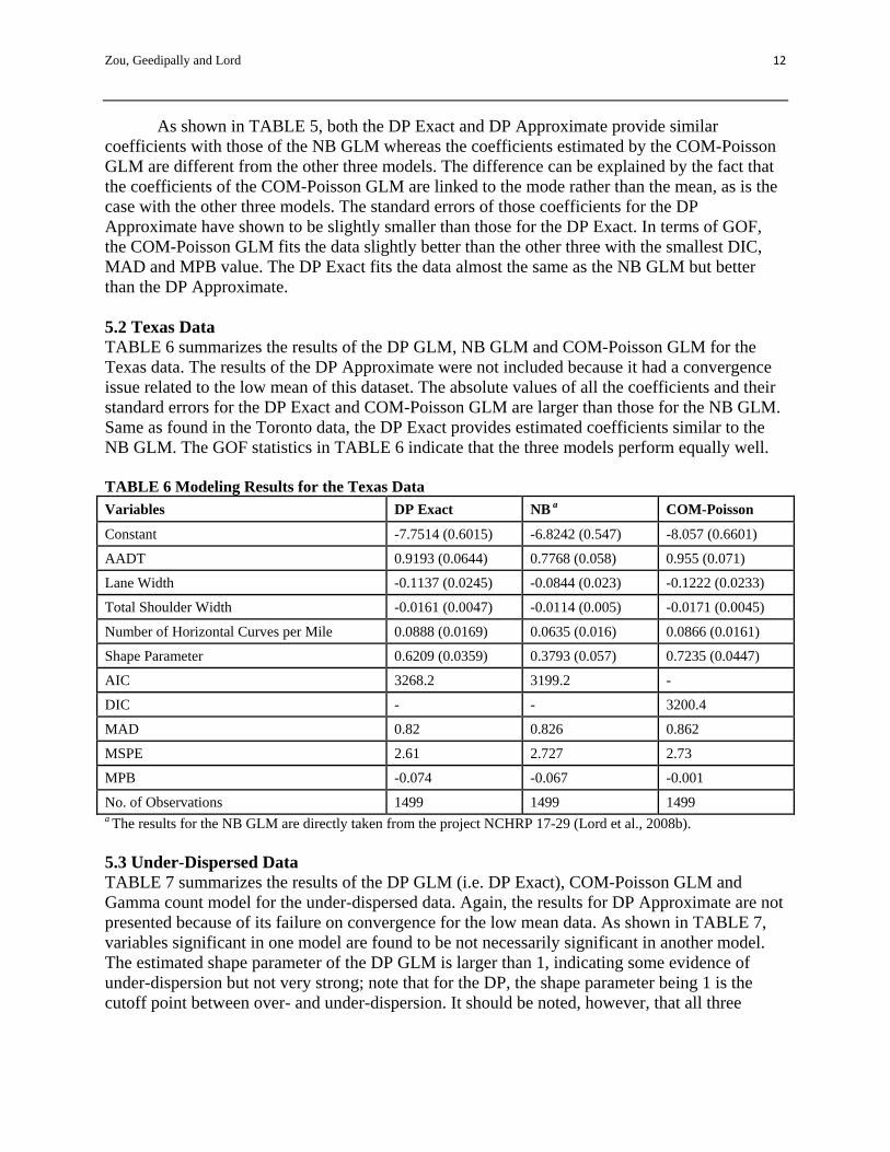
As shown in TABLE 5, both the DP Exact and DP Approximate provide similar coefficients with those of the NB GLM whereas the coefficients estimated by the COM-Poisson GLM are different from the other three models. The difference can be explained by the fact that the coefficients of the COM-Poisson GLM are linked to the mode rather than the mean, as is the case with the other three models. The standard errors of those coefficients for the DP Approximate have shown to be slightly smaller than those for the DP Exact. In terms of GOF, the COM-Poisson GLM fits the data slightly better than the other three with the smallest DIC, MAD and MPB value. The DP Exact fits the data almost the same as the NB GLM but better than the DP Approximate. 5.2 Texas Data TABLE 6 summarizes the results of the DP GLM, NB GLM and COM-Poisson GLM for the Texas data. The results of the DP Approximate were not included because it had a convergence issue related to the low mean of this dataset. The absolute values of all the coefficients and their standard errors for the DP Exact and COM-Poisson GLM are larger than those for the NB GLM. Same as found in the Toronto data, the DP Exact provides estimated coefficients similar to the NB GLM. The GOF statistics in TABLE 6 indicate that the three models perform equally well. TABLE 6 Modeling Results for the Texas Data

Variables DP Exact NB a COM-Poisson

Constant -7.7514 (0.6015) -6.8242 (0.547) -8.057 (0.6601)

AADT 0.9193 (0.0644) 0.7768 (0.058) 0.955 (0.071)

Lane Width -0.1137 (0.0245) -0.0844 (0.023) -0.1222 (0.0233)

Total Shoulder Width -0.0161 (0.0047) -0.0114 (0.005) -0.0171 (0.0045)

Number of Horizontal Curves per Mile 0.0888 (0.0169) 0.0635 (0.016) 0.0866 (0.0161)

Shape Parameter 0.6209 (0.0359) 0.3793 (0.057) 0.7235 (0.0447)

AIC 3268.2 3199.2 -

DIC - - 3200.4

MAD 0.82 0.826 0.862

MSPE 2.61 2.727 2.73

MPB -0.074 -0.067 -0.001

No. of Observations 1499 1499 1499 a The results for the NB GLM are directly taken from the project NCHRP 17-29 (Lord et al., 2008b). 5.3 Under-Dispersed Data TABLE 7 summarizes the results of the DP GLM (i.e. DP Exact), COM-Poisson GLM and Gamma count model for the under-dispersed data. Again, the results for DP Approximate are not presented because of its failure on convergence for the low mean data. As shown in TABLE 7, variables significant in one model are found to be not necessarily significant in another model. The estimated shape parameter of the DP GLM is larger than 1, indicating some evidence of under-dispersion but not very strong; note that for the DP, the shape parameter being 1 is the cutoff point between over- and under-dispersion. It should be noted, however, that all three


models are consistent in showing that under-dispersion is present (when conditioned on the mean).

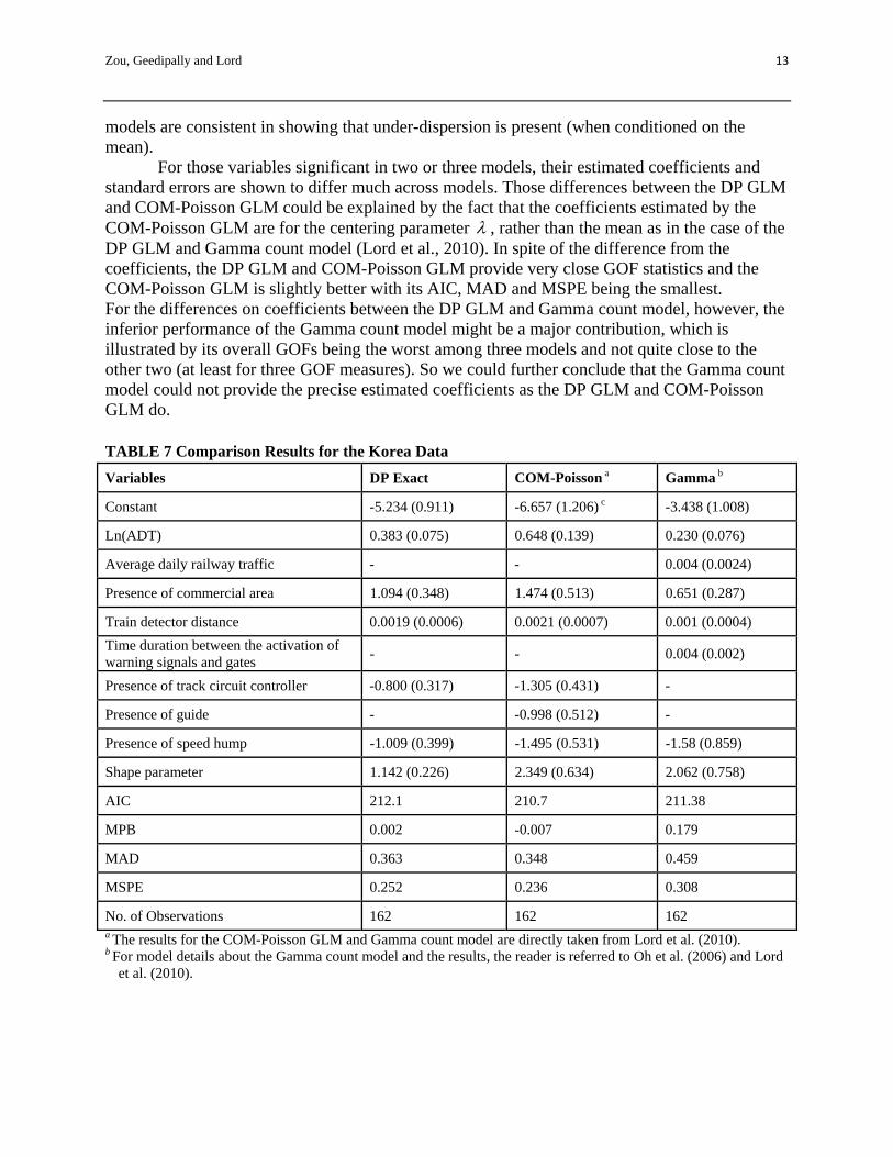
For those variables significant in two or three models, their estimated coefficients and standard errors are shown to differ much across models. Those differences between the DP GLM and COM-Poisson GLM could be explained by the fact that the coefficients estimated by the COM-Poisson GLM are for the centering parameter , rather than the mean as in the case of the DP GLM and Gamma count model (Lord et al., 2010). In spite of the difference from the coefficients, the DP GLM and COM-Poisson GLM provide very close GOF statistics and the COM-Poisson GLM is slightly better with its AIC, MAD and MSPE being the smallest. For the differences on coefficients between the DP GLM and Gamma count model, however, the inferior performance of the Gamma count model might be a major contribution, which is illustrated by its overall GOFs being the worst among three models and not quite close to the other two (at least for three GOF measures). So we could further conclude that the Gamma count model could not provide the precise estimated coefficients as the DP GLM and COM-Poisson GLM do. TABLE 7 Comparison Results for the Korea Data

Variables DP Exact COM-Poisson a Gamma b

Constant -5.234 (0.911) -6.657 (1.206) c -3.438 (1.008)

Ln(ADT) 0.383 (0.075) 0.648 (0.139) 0.230 (0.076)

Average daily railway traffic - - 0.004 (0.0024)

Presence of commercial area 1.094 (0.348) 1.474 (0.513) 0.651 (0.287)

Train detector distance 0.0019 (0.0006) 0.0021 (0.0007) 0.001 (0.0004)

Time duration between the activation of warning signals and gates

- - 0.004 (0.002)

Presence of track circuit controller -0.800 (0.317) -1.305 (0.431) -

Presence of guide - -0.998 (0.512) -

Presence of speed hump -1.009 (0.399) -1.495 (0.531) -1.58 (0.859)

Shape parameter 1.142 (0.226) 2.349 (0.634) 2.062 (0.758)

AIC 212.1 210.7 211.38

MPB 0.002 -0.007 0.179

MAD 0.363 0.348 0.459

MSPE 0.252 0.236 0.308

No. of Observations 162 162 162 a The results for the COM-Poisson GLM and Gamma count model are directly taken from Lord et al. (2010). b For model details about the Gamma count model and the results, the reader is referred to Oh et al. (2006) and Lord

et al. (2010).


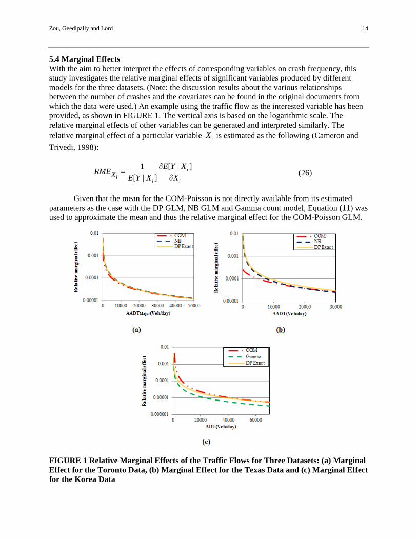
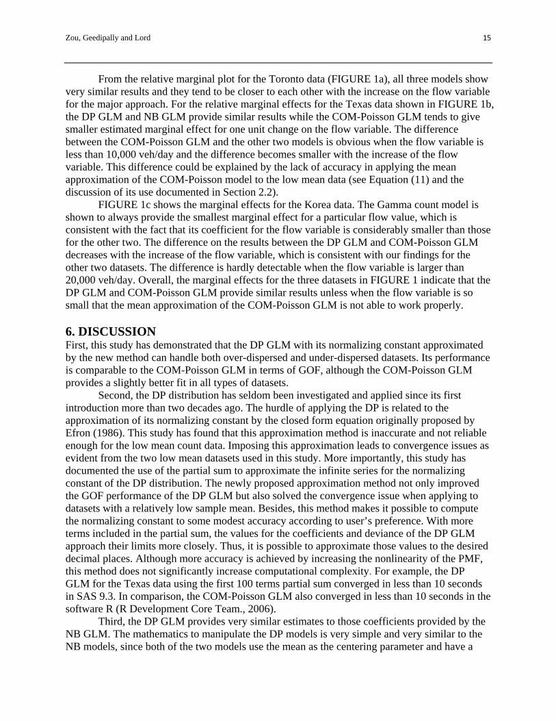
5.4 Marginal Effects With the aim to better interpret the effects of corresponding variables on crash frequency, this study investigates the relative marginal effects of significant variables produced by different models for the three datasets. (Note: the discussion results about the various relationships between the number of crashes and the covariates can be found in the original documents from which the data were used.) An example using the traffic flow as the interested variable has been provided, as shown in FIGURE 1. The vertical axis is based on the logarithmic scale. The relative marginal effects of other variables can be generated and interpreted similarly. The relative marginal effect of a particular variable iX is estimated as the following (Cameron and

Trivedi, 1998):

[ | ]1

[ | ]i

i iiX

E Y XRME

E Y X X

(26)

Given that the mean for the COM-Poisson is not directly available from its estimated

parameters as the case with the DP GLM, NB GLM and Gamma count model, Equation (11) was used to approximate the mean and thus the relative marginal effect for the COM-Poisson GLM.

FIGURE 1 Relative Marginal Effects of the Traffic Flows for Three Datasets: (a) Marginal Effect for the Toronto Data, (b) Marginal Effect for the Texas Data and (c) Marginal Effect for the Korea Data


From the relative marginal plot for the Toronto data (FIGURE 1a), all three models show very similar results and they tend to be closer to each other with the increase on the flow variable for the major approach. For the relative marginal effects for the Texas data shown in FIGURE 1b, the DP GLM and NB GLM provide similar results while the COM-Poisson GLM tends to give smaller estimated marginal effect for one unit change on the flow variable. The difference between the COM-Poisson GLM and the other two models is obvious when the flow variable is less than 10,000 veh/day and the difference becomes smaller with the increase of the flow variable. This difference could be explained by the lack of accuracy in applying the mean approximation of the COM-Poisson model to the low mean data (see Equation (11) and the discussion of its use documented in Section 2.2).

FIGURE 1c shows the marginal effects for the Korea data. The Gamma count model is shown to always provide the smallest marginal effect for a particular flow value, which is consistent with the fact that its coefficient for the flow variable is considerably smaller than those for the other two. The difference on the results between the DP GLM and COM-Poisson GLM decreases with the increase of the flow variable, which is consistent with our findings for the other two datasets. The difference is hardly detectable when the flow variable is larger than 20,000 veh/day. Overall, the marginal effects for the three datasets in FIGURE 1 indicate that the DP GLM and COM-Poisson GLM provide similar results unless when the flow variable is so small that the mean approximation of the COM-Poisson GLM is not able to work properly. 6. DISCUSSION First, this study has demonstrated that the DP GLM with its normalizing constant approximated by the new method can handle both over-dispersed and under-dispersed datasets. Its performance is comparable to the COM-Poisson GLM in terms of GOF, although the COM-Poisson GLM provides a slightly better fit in all types of datasets.

Second, the DP distribution has seldom been investigated and applied since its first introduction more than two decades ago. The hurdle of applying the DP is related to the approximation of its normalizing constant by the closed form equation originally proposed by Efron (1986). This study has found that this approximation method is inaccurate and not reliable enough for the low mean count data. Imposing this approximation leads to convergence issues as evident from the two low mean datasets used in this study. More importantly, this study has documented the use of the partial sum to approximate the infinite series for the normalizing constant of the DP distribution. The newly proposed approximation method not only improved the GOF performance of the DP GLM but also solved the convergence issue when applying to datasets with a relatively low sample mean. Besides, this method makes it possible to compute the normalizing constant to some modest accuracy according to user’s preference. With more terms included in the partial sum, the values for the coefficients and deviance of the DP GLM approach their limits more closely. Thus, it is possible to approximate those values to the desired decimal places. Although more accuracy is achieved by increasing the nonlinearity of the PMF, this method does not significantly increase computational complexity. For example, the DP GLM for the Texas data using the first 100 terms partial sum converged in less than 10 seconds in SAS 9.3. In comparison, the COM-Poisson GLM also converged in less than 10 seconds in the software R (R Development Core Team., 2006).

Third, the DP GLM provides very similar estimates to those coefficients provided by the NB GLM. The mathematics to manipulate the DP models is very simple and very similar to the NB models, since both of the two models use the mean as the centering parameter and have a


shape parameter to capture dispersion. Moreover, both the DP GLM and NB GLM in this study were developed based on the MLE in SAS. However, the application of the NB GLM is only limited to modeling the over-dispersed data and provides unreliable parameter estimates when fitting the under-dispersed data (Lord et al., 2010). On the other hand, the shape parameter of the DP GLM has been found to be very flexible and it can handle under-, equi-, and over-dispersion ( ( ) ( ) /Var Y E Y , 1 for under-dispersion; 1 for equi-dispersion; 1 for over-dispersion). The simplicity and flexibility of the DP mathematics also allows for the further development of multilevel models such as the random parameter models (Anastasopoulos and Mannering, 2009), finite mixture models (Park and Lord, 2009), Markov switching models (Malyshkina et al., 2009), etc., which will better account for the unobserved heterogeneity in crash datasets. This will encourage the potential use of the DP models to handle more complex crash dataset.

Fourth, the DP GLM can be more easily estimated and computationally inexpensive than the COM-Poisson GLM although the former fits the data slightly worse than the latter (at least for these datasets). It is simple to use the DP GLM for interpreting the coefficients in terms of their impact on the mean since the mean parameter is linked to the linear predictor through the logarithmic link. On the other hand, certain mean approximation methods have to be made for applying the COM-Poisson GLM to obtain its mean and thus the marginal effects. However, those approximation methods may not work well for low mean datasets. Previous studies have investigated the accuracy of those approximation methods. For the COM-Poisson GLM based on its original parameterization, the estimated means can be approximated using the asymptotic expression but is only accurate for 1v or 10v (Sellers and Shmueli, 2010). Although the re-parameterization of the COM-Poisson distribution proposed by Guikama and Coffelt (2008) was based on a more clear centering parameter (i.e., the mode), it is still not directly comparable to the mean in the DP GLM.

Despite of the aforementioned advantages of the DP GLM, the application of the DP GLM is associated with several limitations. Due to the scarcity of the observed under-dispersed crash data, this study investigated the performance of the DP GLM using only one observed dataset. Further investigation should be conducted on how the DP GLM will handle under-dispersed count data in a broader context. Besides, to make a fair comparison, the model specifications of the DP GLMs are consistent with those of the COM-Poisson GLMs, which have been documented in past studies. However, doing this does not guarantee the models are not affected by the issue of omitting variable bias. Future work should investigate how including more variables in the model will affect the comparison in terms of performance between these two models, especially for variables that are known to significantly influence the frequency of crashes. Further work is also recommended to better understand under which circumstances the DP GLM is preferred over the COM-Poisson GLM. 7. SUMMARY AND CONCLUSIONS This study has examined the applicability of the DP GLM for analyzing motor vehicle crash data characterized by over- and under-dispersion and compared its performance to that of the COM-Poisson GLM. The DP GLM was developed based on a new method to approximate its normalizing constant with high accuracy and reliability. The normalizing constant of the DP distribution used to be left out or approximated using a closed form formula, and neither of them can provide accurate enough results especially for the low mean data. The DP GLM and COM-


Poisson GLM were developed using two observed over-dispersed datasets and one observed under-dispersed dataset. The results of the NB GLM and Gamma count model were also provided as reference.

The modeling results for both over- and under-dispersed datasets indicate that the DP GLM with its normalizing constant approximated by the new method performs slightly worse than the COM-Poisson GLM in terms of the GOF statistics. The differences, however, are not large enough to disregard its use for analyzing crash data. Indeed, the former is much easier to use and estimate than the latter. The coefficients in terms of their impact on the means are simpler to interpret with the DP GLM than for the COM-Poisson GLM. The computational time needed for the DP GLM to converge is so small that it only takes several seconds to generate the modeling results. In sum, the DP GLM with its properly approximated normalizing constant offers a very flexible and efficient alternative for researchers for modeling count data.

ACKNOWLEDGEMENTS The authors would like to thank Dr. Thomas Wehrly from Texas A&M University for his insightful statistics-related comments. REFERENCES Anastasopoulos, P., Mannering, F., 2009. A note on modeling vehicle-accident frequencies with

random-parameters count models. Accident Analysis and Prevention 41 (1), 153-159. Borle S, Boatwright P, Kadane JB., 2006. The timing of bid placement and extent of multiple

bidding: An empirical investigation using eBay online auctions. Statistical Science, 21(2):194-205.

Cameron, A.C., Trivedi, P.K., 1998. Regression Analysis of Count Data. Cambridge University Press, Cambridge, UK.

Castillo, J and Perez-Casany,M., 2005. Over-dispersed and under-dispersed Poisson generalizations. Journal of Statistical Planning and Inference 134 (2), 486-500.

Consul, P.C., 1989. Generalized Poisson Distributions: Properties and Applications, Marcel Dekker, New York.

Conway, R.W., Maxwell, W.L., 1962. A queuing model with state dependent service rates. Journal of Industrial Engineering 12, 132-136.

Efron, B., 1986. Double exponential families and their use in generalized linear Regression. Journal of the American Statistical Association 81 (395), 709-721.

Famoye, F., 1993. Restricted generalized Poisson regression model. Communications in Statistics - Theory and Methods 22 (5), 1335-1354.

Francis, R.A., Geedipally, S.R., Guikema, S.D., Dhavala, S.S., Lord, D., and Larocca, S., 2012. Characterizing the performance of the Conway-Maxwell-Poisson generalized linear model. Risk Analysis 32 (1), 167-183.

Guikema, S.D., Coffelt, J.P., 2008. A flexible count data regression model for risk analysis. Risk Analysis 28 (1), 213-223.

Hauer, E., 1997. Observation Before-After Studies in Road Safety: Estimating the Effect of Highway and Traffic Engineering Measures on Road Safety. Elsevier Science Ltd., Oxford.

Hilbe, J.M., 2011. Negative Binomial Regression (Second Edition). Cambridge University Press, Cambridge, UK.

Kadane, J.B., Shmueli, G., Minka, T.P., Borle, S., Boatwright, P., 2006. Conjugate analysis of the Conway–Maxwell–Poisson distribution. Bayesian Analysis 1, 363–374.


Lord, D., 2000. The prediction of accidents on digital networks: characteristics and issues related to the application of accident prediction models. Ph.D. dissertation, Department of Civil Engineering, University of Toronto, Toronto, Ontario.

Lord, D., Geedipally, S.R., Guikema, S., 2010. Extension of the application of Conway-Maxwell-Poisson models: analyzing traffic crash data exhibiting under-dispersion. Risk Analysis, 30 (8) 1268-1276.

Lord, D., Geedipally, S.R., Persaud, B.N., Washington, S.P., van Schalkwyk, I., Ivan, J.N., Lyon, C., Jonsson, T., 2008b. Methodology for estimating the safety performance of multilane rural highways. NCHRP Web-Only Document 126, National Cooperation Highway Research Program, Washington, D.C. (http://onlinepubs.trb.org/onlinepubs/nchrp/nchrp w126.pdf, retrieved on February 2012).

Lord, D., Guikema, S.D., Geedipally, S.R., 2008a. Application of the Conway-Maxwell-Poisson generalized linear model for analyzing motor vehicle crashes. Accident Analysis and Prevention 40 (3), 1123-1134.

Lord, D., Mannering, F.L., 2010. The statistical analysis of crash-frequency data: a review and assessment of methodological alternatives. Transportation Research Part A: Policy and Practice 44 (5), 291-305.

Malyshkina, N., Mannering, F., Tarko, A., 2009. Markov switching negative binomial models: An application to vehicle accident frequencies. Accident Analysis and Prevention 41 (2), 217-226.

Miaou, S.-P., Lord, D., 2003. Modeling traffic crash-flow relationships for intersections: dispersion parameter, functional form, and Bayes versus empirical Bayes. Transportation Research Record 1840, 31-40.

Oh, J., Lyon, C., Washington, S.P., Persaud, B.N., Bared, J. 2003. Validation of the FHWA Crash Models for Rural Intersections: Lessons Learned. Transportation Research Record 1840, 41-49.

Oh, J., Washington, S.P., Nam, D., 2006. Accident prediction model for railway-highway interfaces. Accident Analysis & Prevention 38 (2), 346-356.

Park, B.-J., Lord, D., 2009. Application of finite mixture models for vehicle crash data analysis Accident Analysis and Prevention 41 (4), 683–691.

Park, E.S., Lord D., 2007. Multivariate Poisson-Lognormal Models for Jointly Modeling Crash Frequency by Severity. Transportation Research Record 2019, 1-6.

R Development Core Team., 2006. R: A language and environment for statistical computing. R Foundation for Statistical Computing, Vienna, Austria. ISBN 3-900051-07-0.

SAS Institute Inc., 2002. Version 9 of the SAS System for Windows. Cary, NC. Sellers, K. F., Borle, S., Shmueli, G., 2012. The COM-Poisson model for count data: a survey of

methods and applications. Applied Stochastic Models in Business and Industry 28 (2). Shmueli, G., Minka, T.P., Kadane, J.B., Borle, S., Boatwright, P., 2005. A useful distribution for

fitting discrete data: revival of the Conway–Maxwell–Poisson distribution. Journal of the Royal Statistical Society, Part C 54, 127-142.

Spiegelhalter, D.J., Thomas, A., Best, N.G., Lun, D., 2003. WinBUGS Version 1.4.1 User Manual. MRC Biostatistics Unit, Cambridge. Available from: <http://www.mrcbsu.cam.ac.uk/bugs/welcome.shtml>.

Sellers, K.F. and Shmueli, G., 2010. A flexible regression model for count data. Annals of Applied Statistics 4 (2), 943-961.


Winkelmann, R., 2008. Econometric Analysis of Count Data (Fifth Edition). Springer-Verlag, Berlin.

Zhu, F., 2012. Modeling Time Series of Counts with COM-Poisson INGARCH Models. Mathematical and Computer Modelling 56 (9), 191-203.

Documents

Evaluating the Double Poisson Generalized Linear Model · PDF fileEvaluating the Double Poisson Generalized Linear Model Yaotian Zou1 Research Assistant ... The hurdle of applying