Journal of Environmental Protection, 2016, 7, 1522-1546 http://www.scirp.org/journal/jep

ISSN Online: 2152-2219 ISSN Print: 2152-2197

DOI: 10.4236/jep.2016.711127 October 27, 2016

Evaluating the Economic and Environmental Impacts of a Global GMO Ban

Harry Mahaffey1, Farzad Taheripour2*, Wallace E. Tyner2

1Cargill, Kansas City, USA 2Department of Agricultural Economics, Purdue University, West Lafayette, IN, USA

Abstract The objective of this research is to assess the global economic and greenhouse gas emission impacts of banning GMO crops. This is done by modeling two counterfac-tual scenarios and evaluating them apart and in combination using a well-know Computable General Equilibrium (CGE) model, GTAP-BIO. The first scenario mod-els the impact of a global GMO ban. The second scenario models the impact of in-creased GMO penetration. The focus is on the price and welfare impacts, and land use change greenhouse gas (GHG) emissions associated with GMO technologies. Much of the prior work on the economic impacts of GMO technology has relied on a combination of partial equilibrium analysis and econometric techniques. However, CGE modelling is a way of analyzing economy-wide impacts that take into account the linkages in the global economy. Here the goal is to contribute to the literature on the benefits of GMO technology by estimating the impacts on price, supply and wel-fare. Food price impacts range from an increase of 0.27% to 2.2%, depending on the region. Total welfare losses associated with loss of GMO technology total up to $9.75 billion. The loss of GMO traits as an intensification technology has not only eco-nomic impacts, but also environmental ones. The full environmental analysis of GMO is not undertaken here. Rather we model the land use change owing to the loss of GMO traits and calculate the associated increase in GHG emissions. We predict a substantial increase in GHG emissions if GMO technology is banned.

Keywords GMO Crops, Productivity, Computable General Equilibrium, Economic Impacts, Land Use Change

1. Introduction

Genetically modified organism (GMO) is defined as one being produced via genetic

How to cite this paper: Mahaffey, H., Tahe-ripour, F. and Tyner, W.E. (2016) Evaluating the Economic and Environmental Impacts of a Global GMO Ban. Journal of Environ-mental Protection, 7, 1522-1546. http://dx.doi.org/10.4236/jep.2016.711127 Received: August 15, 2016 Accepted: October 24, 2016 Published: October 27, 2016 Copyright © 2016 by authors and Scientific Research Publishing Inc. This work is licensed under the Creative Commons Attribution International License (CC BY 4.0). http://creativecommons.org/licenses/by/4.0/

Open Access

H. Mahaffey et al.

1523

modification as contrasted with conventional breeding [1]. GMO crops have been a lightning rod for controversy since their introduction into agriculture in the early 1990s. With the development of commercially viable genetically modified field crops (insect resistant corn and herbicide tolerant soybeans in particular), the controversy only in-tensified. Indeed the controversy is such that some public intellectuals including but not limited to economists, biologists, and philosophers have taken sides in the debate on GMO crops (examples are: Taleb et al. [2], Dawkins [3], Singer and Daar [4]). Con-sumer fears about the danger of GMO crops including fears about the safety of geneti-cally modified food for human consumption, the impact of GMO crops on the envi-ronment, and the effect of GMO crops on farms and farmers. These fears, along with some economic considerations, have led to significant regulatory obstacles to GMO crops worldwide.

However, consumer concerns are not paramount in the peer-reviewed literature on the subject. Rather, the evidence from agronomy, biology and public health indicates that GMO crops are not dangerous, and the evidence from economics shows that GMO crops are associated with positive economic outcomes, including for the poorest people. Many consumers in developed countries demonstrate a clear preference for non-GMO crops. A pretty substantial body of research exists around this subject. A large piece of it focuses on quantifying consumer’s preferences for non-GMO. This has included wil-lingness-to-pay and willingness-to-accept analysis of consumer preference in various countries. Fernandez-Cornejo et al. [5] provide an overview of much of the research done in this area. Following Lusk et al. [6], they conclude that while many consumers are willing to pay a premium for non-GMO foods, a good deal depends on where the study is being performed. Lusk et al. [6] perform a meta-analysis of studies focused on GM vs. non-GM valuation.

That many consumers prefer non-genetically engineered varieties is not truly up for debate. What explains this preference is less clear. Part of the explanation seems to be that consumers do not just prefer non-GMO products, but actually fear the effects of genetic modification. Chiang et al. [7] report that a substantial percentage of consumers across the world believe that GMO crops are dangerous for human consumption. In a more recent study, Costa-Font and Mossialos [8] suggest that what they term dread of GMO crops is at least partially explained by lack of information. In the absence of in-formation, consumers adopt a self-protective attitude that here is expressed as an an-ti-GMO attitude. This suggests that the preference for non-GMO emerges from a fail-ure to communicate on the part of GMO advocates. In other work, Costa-Font and Gil [9] have found that meta-attitudes about science and technology can also explicate at-titudes towards GMO crops.

The picture of why consumers distrust and dis-prefer GMO crops and genetically engineered food is a complex one. Whatever the explanation, consumer fear of GMO crops and preference for non-GMO varieties is a fact. This is reflected in global agri-cultural policy. GMO crops are heavily regulated everywhere in the world, with partial or full bans on cultivation in many European and Asian countries. In China, according

H. Mahaffey et al.

1524

to the ISAA, there is only one variety of GMO maize approved for cultivation, and no varieties of GMO soybeans. There are a larger number of varieties approved for im-port, though imports tainted by unapproved varieties have been a source of some con-tention [10] [11]. In Europe there are a variety of regulatory attitudes. In the EU in general, it is legal to import GMO crops and feed, so long as the GMO variety is one of the approved varieties. If shipments are found that include a certain percentage of an unapproved GMO variety, the shipment is refused [11]. The EU also approves a cer-tain number of GMO crops, though the individual member states are allowed to opt- out, through a variety of regulatory mechanisms. France and Germany have outright bans on growing GMO crops of any kind. Spain and the Czech Republic, on the other hand grow approved GMO crops in significant percentages. The United States is the world’s leader in GMO crop planting and in the development of agricultural biotech-nology. Indeed it is only very recently that the rest of the worlds’ GMO planted acreage overtook the United States [12]. According to the ISAA, there are currently 189 GMO varieties currently approved for cultivation in the United States (across a wide variety of crops). Regulation of GMO crops is managed by three federal agencies: The Environmental Protection Agency, the Department of Agriculture and the Food and Drug Administration [13]. Though the United States is the largest producer and user of GMO technology, there continues to be resistance and opposition to GMO crops. Most recently, legislation around GMO labeling requirements has been a locus [14].

In what follows, we examine two distinct counterfactual scenarios. Both use the 2013 yield improvement estimates from Brookes and Barfoot’s data [15]. The first asks, “What would be different if there was no GMO technology?” The second asks, “What would be the impact if GMO adoption globally caught up to the United States?” By examining these scenarios individually as well as in combination, we can determine the economic and environmental impacts of banning GMO crops.

The first scenario is the most straightforward. It assumes that GMO penetration is exactly what it was as of 2013 in each region. This case asks what would be the eco-nomic and GHG impacts of switching from GMO to conventional, assuming that GMO crops would remain at their current level of penetration.

In the second scenario, we model the effects of increasing the penetration of GMO crops in the rest of the world to the penetration rate achieved in the US. This in turn provides a picture of the as yet unrealized potential benefits of GMO crops. While the first scenario asks “How much better off are we?”, the second asks “How much better off could we be?”

The only countries included in the second scenario are countries with GMO crops already planted. Obviously, it is possible that other countries in the future will permit GMO varieties, so our analysis represents a very conservative estimate of GMO benefits. While other countries likely would benefit from GMO crops, policy is political, not strictly economic. Thus, the estimates provided assume no complete policy changes from cur-rent policy.

H. Mahaffey et al.

1525

2. Yield Contributions of GMO Crops

The data used for this study consists in a set of yield shocks for the three main GMO crops (soybeans, corn, and cotton) by country. These crops were chosen because they represent the vast majority of GMO acreage planted [12]. They are also the three crops with the fullest global data [15] and the greatest global economic impacts [16] [17]. The basic yield shock assumptions are drawn from Brookes and Barfoot [15] [18] review of the literature. These numbers are then combined with data on current GMO penetra-tion in the United States and the rest of the world in order to produce estimates of rea-listic yield shocks by crop and country.

2.1. Derivation of Yield Shocks

The literature on yield impacts of GMO crops used in this work derives the yield im-provement associated with GE traits. In order to derive shocks usable in the GTAP model, we must first derive the yield shocks for each trait. These are weighted by area, and the overall yield impact of GMO technology for the crop is determined. Finally, these weighted yield shocks are weighted according to the crop share in the GTAP crop grouping and an adjustment for regional aggregation. The derivation follows.

We define the yield of some country, Y, as the sum of the conventional yield and the GMO yield, weighted by their respective penetrations. Penetration here is understood as the proportion of the total area planted to each variety and is defined such that,

1c gP P= − (1)

where cP is the penetration of conventional varieties and gP is the penetration of GMO varieties. The yield of the GMO varieties is defined in terms of the yield of con-ventional varieties and the GMO yield improvement such that,

( )1g c iY Y Y= × + (2)

where gY is the GMO yield, cY is the conventional yield and iY is the yield im-provement. Thus by (1) and (2), (3) and (4) can be shown to be equivalent.

c c g gY Y P Y P= × + × (3)

( )1c i gY Y Y P= + . (4)

Thus we have derived current yield in terms of conventional yield, GMO yield im-provement and GMO penetration. In our first scenario, our aim is to determine the impact of switching over exclusively to conventional crops. In order to do so, we define an x such that

cx Y Y× = . (5)

That is, x is the fraction of the original yield obtained if GMO varieties are no longer available. By plugging in the identity in Equation (4), we put x in terms of yield im-provement and GMO penetration.

11 i g

xY P

=+

. (6)

H. Mahaffey et al.

1526

Equation (7) is equivalent to Equation (6), and gives the yield loss associated with switching over to exclusively conventional crops.

11

i g

i g

Y Px

Y P−

− =+

. (7)

Thus for instance, if the yield without any GMO crops would be 96% of current yield, then that counterfactual yield is 0.96% - 1% = −4% lower than current yield.

We consider also a scenario in which penetration of GMO crops increases. Our goal is to derive the change in yield given the change in penetration, yield improvement and the original penetration. We assume that only penetration changes-conventional and GMO yield remain as they were. The change in yield is given by Equation (8).

( ) ( )2 1 2 11 1c i g c i gY Y Y Y P Y Y P− = + − + (8)

where 2Y is the yield after increased penetration and 1Y is the current yield, with 2gP and 1gP the respective penetrations. Equation (8) simplifies to Equation (9).

( )2 1c i g gY Y Y P P∆ = − . (9)

From Equation (4) and Equation (9), we derive Equation (10).

( )( )

2 11

11i g g

i g

Y P PY Y

Y P

−∆ = ×

+. (10)

Thus the positive yield shock given an increase in penetration from 1gP to 2gP is as given in Equation (11).

( )( )

2 1

11i g g

si g

Y P PY

Y P

−=

+ (11)

where sY is the positive yield shock. GMO crops do not always include only one trait. Indeed, in the United States, a ma-

jority of the corn (~75% [5]) is stacked-trait. A single cultivar might include several kinds of insect resistance and herbicide resistance. There are three possibilities for inte-raction effects in GE traits-the trait impacts can be additive, more than additive or less than additive. The implicit assumption in Brookes and Barfoot’s work is that the traits are additive. Given the damage control framework for thinking about yield improve-ment [19], additivity is a reasonable simplifying assumption. Thus the yield shock by crop for each country is simply the sum of the total yield shocks of every trait for a giv-en crop. This is expressed in Equation (12).

i g a a b b n nY P Y P Y P Y P= + + + (12)

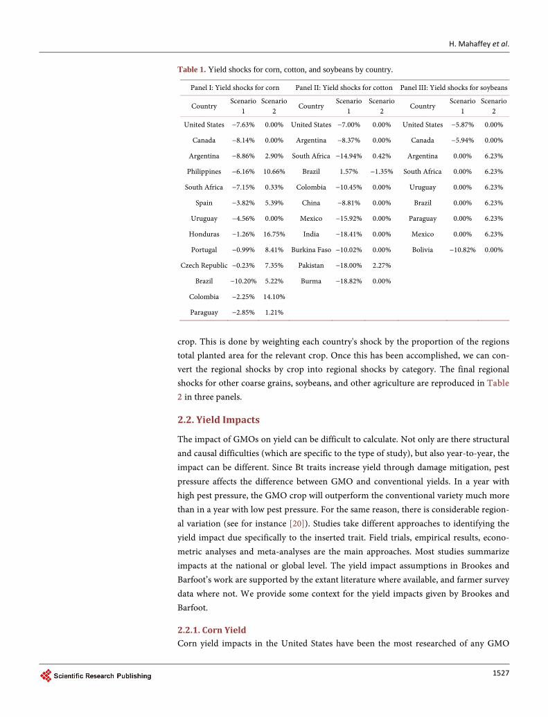
where jY is the yield improvement associated with some trait j and jP is the pene-tration of that trait. Panels I, II, and III of Table 1 give the weighted yield shocks for corn, cotton, and soybeans by country.

These country shocks must then be converted into GTAP shocks. This happens in two steps. GTAP aggregates countries into regions and aggregates crops into categories. The first step, then, is to convert the country shocks by crop into regional shocks by

H. Mahaffey et al.

1527

Table 1. Yield shocks for corn, cotton, and soybeans by country.

Panel I: Yield shocks for corn Panel II: Yield shocks for cotton Panel III: Yield shocks for soybeans

Country Scenario

1 Scenario

2 Country

Scenario 1

Scenario 2

Country Scenario

1 Scenario

2

United States −7.63% 0.00% United States −7.00% 0.00% United States −5.87% 0.00%

Canada −8.14% 0.00% Argentina −8.37% 0.00% Canada −5.94% 0.00%

Argentina −8.86% 2.90% South Africa −14.94% 0.42% Argentina 0.00% 6.23%

Philippines −6.16% 10.66% Brazil 1.57% −1.35% South Africa 0.00% 6.23%

South Africa −7.15% 0.33% Colombia −10.45% 0.00% Uruguay 0.00% 6.23%

Spain −3.82% 5.39% China −8.81% 0.00% Brazil 0.00% 6.23%

Uruguay −4.56% 0.00% Mexico −15.92% 0.00% Paraguay 0.00% 6.23%

Honduras −1.26% 16.75% India −18.41% 0.00% Mexico 0.00% 6.23%

Portugal −0.99% 8.41% Burkina Faso −10.02% 0.00% Bolivia −10.82% 0.00%

Czech Republic −0.23% 7.35% Pakistan −18.00% 2.27%

Brazil −10.20% 5.22% Burma −18.82% 0.00%

Colombia −2.25% 14.10%

Paraguay −2.85% 1.21%

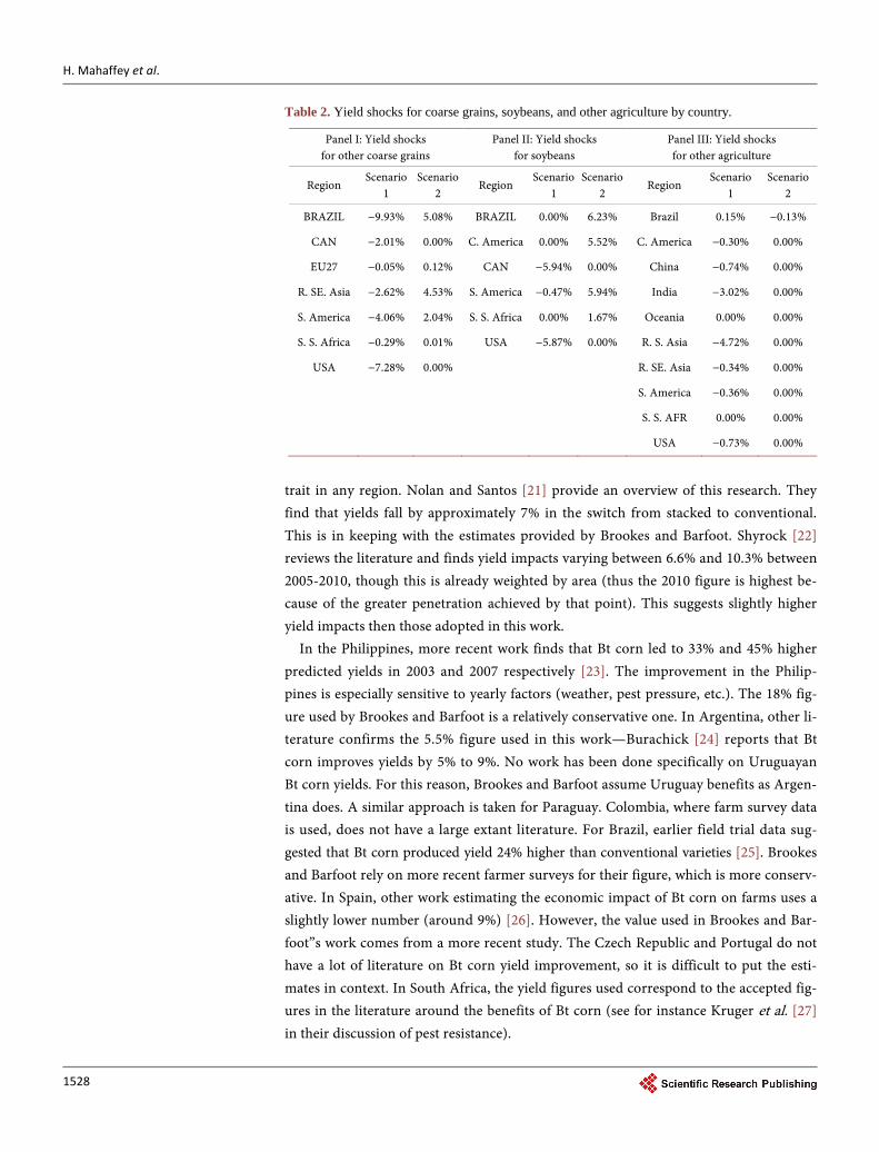
crop. This is done by weighting each country's shock by the proportion of the regions total planted area for the relevant crop. Once this has been accomplished, we can con-vert the regional shocks by crop into regional shocks by category. The final regional shocks for other coarse grains, soybeans, and other agriculture are reproduced in Table 2 in three panels.

2.2. Yield Impacts

The impact of GMOs on yield can be difficult to calculate. Not only are there structural and causal difficulties (which are specific to the type of study), but also year-to-year, the impact can be different. Since Bt traits increase yield through damage mitigation, pest pressure affects the difference between GMO and conventional yields. In a year with high pest pressure, the GMO crop will outperform the conventional variety much more than in a year with low pest pressure. For the same reason, there is considerable region-al variation (see for instance [20]). Studies take different approaches to identifying the yield impact due specifically to the inserted trait. Field trials, empirical results, econo-metric analyses and meta-analyses are the main approaches. Most studies summarize impacts at the national or global level. The yield impact assumptions in Brookes and Barfoot’s work are supported by the extant literature where available, and farmer survey data where not. We provide some context for the yield impacts given by Brookes and Barfoot.

2.2.1. Corn Yield Corn yield impacts in the United States have been the most researched of any GMO

H. Mahaffey et al.

1528

Table 2. Yield shocks for coarse grains, soybeans, and other agriculture by country.

Panel I: Yield shocks for other coarse grains

Panel II: Yield shocks for soybeans

Panel III: Yield shocks for other agriculture

Region Scenario

1 Scenario

2 Region

Scenario 1

Scenario 2

Region Scenario

1 Scenario

2

BRAZIL −9.93% 5.08% BRAZIL 0.00% 6.23% Brazil 0.15% −0.13%

CAN −2.01% 0.00% C. America 0.00% 5.52% C. America −0.30% 0.00%

EU27 −0.05% 0.12% CAN −5.94% 0.00% China −0.74% 0.00%

R. SE. Asia −2.62% 4.53% S. America −0.47% 5.94% India −3.02% 0.00%

S. America −4.06% 2.04% S. S. Africa 0.00% 1.67% Oceania 0.00% 0.00%

S. S. Africa −0.29% 0.01% USA −5.87% 0.00% R. S. Asia −4.72% 0.00%

USA −7.28% 0.00% R. SE. Asia −0.34% 0.00%

S. America −0.36% 0.00%

S. S. AFR 0.00% 0.00%

USA −0.73% 0.00%

trait in any region. Nolan and Santos [21] provide an overview of this research. They find that yields fall by approximately 7% in the switch from stacked to conventional. This is in keeping with the estimates provided by Brookes and Barfoot. Shyrock [22] reviews the literature and finds yield impacts varying between 6.6% and 10.3% between 2005-2010, though this is already weighted by area (thus the 2010 figure is highest be-cause of the greater penetration achieved by that point). This suggests slightly higher yield impacts then those adopted in this work.

In the Philippines, more recent work finds that Bt corn led to 33% and 45% higher predicted yields in 2003 and 2007 respectively [23]. The improvement in the Philip-pines is especially sensitive to yearly factors (weather, pest pressure, etc.). The 18% fig-ure used by Brookes and Barfoot is a relatively conservative one. In Argentina, other li-terature confirms the 5.5% figure used in this work—Burachick [24] reports that Bt corn improves yields by 5% to 9%. No work has been done specifically on Uruguayan Bt corn yields. For this reason, Brookes and Barfoot assume Uruguay benefits as Argen-tina does. A similar approach is taken for Paraguay. Colombia, where farm survey data is used, does not have a large extant literature. For Brazil, earlier field trial data sug-gested that Bt corn produced yield 24% higher than conventional varieties [25]. Brookes and Barfoot rely on more recent farmer surveys for their figure, which is more conserv-ative. In Spain, other work estimating the economic impact of Bt corn on farms uses a slightly lower number (around 9%) [26]. However, the value used in Brookes and Bar-foot”s work comes from a more recent study. The Czech Republic and Portugal do not have a lot of literature on Bt corn yield improvement, so it is difficult to put the esti-mates in context. In South Africa, the yield figures used correspond to the accepted fig-ures in the literature around the benefits of Bt corn (see for instance Kruger et al. [27] in their discussion of pest resistance).

H. Mahaffey et al.

1529

2.2.2. Soybean Yield The assumption that first generation soybeans provide no yield advantage in most of the world is consistent across the literature. In general, herbicide tolerance provides no yield improvement. The adoption of herbicide tolerant soybeans is not a function of yield improvement, but rather a function of cost and time savings [28] [29]. There are only two assumptions made by Brookes and Barfoot with respect to soybean yields. The first is that farmers in the United States who have planted second generation soybeans have experienced yield gains [15]. The technology is new, so there is not a large amount of data yet available for the rest of the world. The second is that Bolivia experiences a yield improvement with herbicide tolerant soybeans. This is confirmed in further work by Smale et al. on the impact of soybeans in Bolivia [30].

2.2.3. Cotton Yield In the United States, there are two major types of Bt cotton planted: Bollgard 1 and Bollgard 2. The figures used by Brookes and Barfoot are conservative. They use yield increases around 10%, which corresponds to work by Verhalen et al. [31]. Other pieces of the literature support yield increases from 15% up to 25% and even higher depend-ing on year and region [20] [32] [33]. In Argentina, the primary work done on yield improvement in cotton is the work cited by Brookes and Barfoot. However, they ac-knowledge using the lower of the estimates in the data (30% yield improvement) rather than the higher numbers found in Qaim and De Janvry (35% yield improvement) [34]. Brazil's figures are based on as yet unpublished farm survey data—it is therefore diffi-cult to put the figures into context. In Colombia, the figures used in this work are con-servative.

Earlier farm survey work found an average yield improvement of 35% for Bt over conventional [35]. In Mexico, the main work on GMO yield improvement for cot-ton was done by Traxler, who noted in 2004 that the improvements due to GMO are highly variable year to year [36]. In South Africa, econometric analysis by Gouse et al. [37] find varying yield improvements for Bt cotton depending on farm size. These improvements range from around 14% to around 46%. Other work using farm survey data found farmers using GMO varieties obtained yields at least 56% greater than farmers using conventional varieties through three seasons of planting [38]. The work on GMO yield improvement in Burkina Faso is the work cited in Brookes and Barfoot’s data—there is no other literature to put these numbers in context. In China, the figures used here align with the overall consensus—that China expe-riences roughly 10% yield improvement for Bt over conventional varieties [39]. Some work finds slightly lower figures, closer to 6% [40]. The difference can be explained by regional and seasonal differences in the data being used. In India, earlier work found GMO yield improvements of 37% on average across three seasons [41]. Oth-er studies confirm this magnitude of yield improvement [42], though some work points to even higher yield improvements (80%) [43]. In Pakistan, the yield im-provement for Bt over conventional used here is in line with other empirical analy-sis [44].

H. Mahaffey et al.

1530

3. Modeling Framework 3.1. Computable General Equilibrium

Computable General Equilibrium (CGE) models are economic models that attempt to solve for the equilibrium conditions in the economy, by modeling the behaviors of three agents: households, firms, and the government. Based on the assumptions about these behaviors (e.g. profit maximizing firms, or utility maximizing households), a CGE model determines demands for and supplies of goods and services endogenously, while it takes into account resource constrains. The CGE models stand in contrast to partial equilibrium models in the way they approach the relationships among markets. In par-tial equilibrium models, the focus is commonly on a single market or a few markets in isolation from the other parts of the economy. In general equilibrium analyses, the goal is to determine the equilibrium conditions across the whole global economy. This means accounting for linkages across markets in an economy including both product and fac-tor markets is much more important in general equilibrium approaches. The CGE mod-els are used for economy-wide analysis. They are necessarily built out of input-output tables representing all goods and services produced, consumed, and traded given pri-mary factors of production including labor, land, capital, and resources. A typical in-put-output table represents the extent to which industries are reliant on the outputs of other industries. It also captures the links between the economic agents represented in the model: firms, households, and the government. Together these tools arguably cap-ture the linkages that characterize specific economies. Another important piece of any CGE model are the elasticities—these parameters capture a wide variety of responses to change across an economy (for instance, relevant here are elasticities that capture the conversion of land in response to changing agricultural commodity prices).Obviously solving for the global general equilibrium requires a considerable amount of data and computational power.

3.2. GTAP-BIO Model

The model used in this work is an extension of the Global Trade Analysis Project (GTAP) framework developed originally by Thomas Hertel [45]. There are two parallel features of GTAP: the model, which attempts to capture the structural features of the global economy and the database built from social accounting matrices for countries that are then aggregated by region. The GTAP database is unique. It contains country input and output data, along with other empirical data representing relationships among markets and industries, and relationships between countries. The database is updated periodi-cally, and new versions are created that attempt to capture the most up to date informa-tion on the state of the global economy. It is worth noting that the GTAP model used in this paper is a comparative static model-thus we are comparing the current economic situation to the economic situation given certain changes. The changes are not changes “over time” but rather counterfactual comparisons. Since its creation, a number of ad-vancements, both in the modeling techniques and in the collection of data have made GTAP one of the preeminent CGE modeling frameworks and data bases. The informa-

H. Mahaffey et al.

1531

tion for the GTAP database is drawn from a number of sources. These include the World Bank, the UN Statistics Division, as well as individual country’s statistic’s de-partments. Some of these advancements include the disaggregation of land by agro- ecological zone (AEZ) [46].

As biofuels began to experience a revival in interest and production (based on the aggressive goals of the Renewable Fuel Standard), they were integrated into both the GTAP database and model, leading to the GTAP-BIO model [47]. This version of the model and the database capture not just the biofuels themselves, but also the secondary byproducts of biofuel production (e.g. dried distiller’s grains). This model was subse-quently used to quantify the economic and environmental impacts not just of agricul-tural policy and trade policy, but also of a variety of other kinds of public policy (energy, water, etc.) [48]-[50].

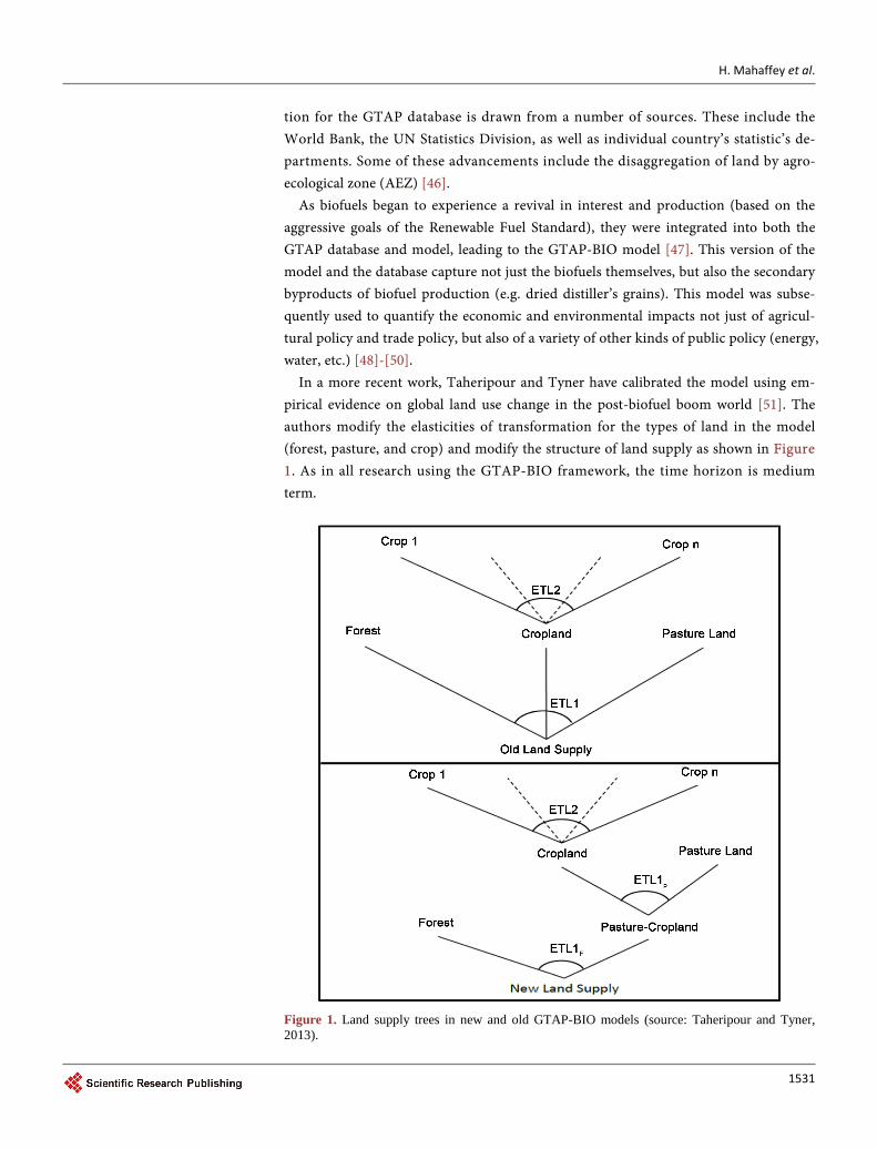
In a more recent work, Taheripour and Tyner have calibrated the model using em-pirical evidence on global land use change in the post-biofuel boom world [51]. The authors modify the elasticities of transformation for the types of land in the model (forest, pasture, and crop) and modify the structure of land supply as shown in Figure 1. As in all research using the GTAP-BIO framework, the time horizon is medium term.

Figure 1. Land supply trees in new and old GTAP-BIO models (source: Taheripour and Tyner, 2013).

H. Mahaffey et al.

1532

In the original model, all land use types are in the same nest-the assumption under-lying this decision is that forest and pasture have the same ease of transformation to cropland. The new two-level nest implicitly assumes that pasture is easier and less ex-pensive to convert than forest.

The two level nest version of the model is used in this work. Using this model allows us to account for the effect of GMO yield shocks on land use change in the presence of global biofuel production. It also allows us to quantify more accurately the land use impacts of falling yields, which is of critical importance for this work.

The database used in this work is the most recent available. It represents the global economy in 2011. There are 19 regions, some of which are composed of individual countries, others of which aggregate country level data. Goods and services are aggre-gated into 52 categories, which include individual commodities (e.g. soybeans) as well as aggregated categories (e.g. coarse grains).

3.3. Implemented Closure

Only two major modifications to the model’s closure are made. The first is required in order to shock yields, and mostly technical. The basic model sets a limited number of variables as exogenous, with the rest being determined by the model (or endogenously). Since yield is not one of the exogenous variables, we swap yield with a technological change variable that is exogenous. The other modification is that biofuel production is fixed in the EU, Brazil and the United States at their base level. These three regions produce the vast majority of global biofuels in the 2011 database (approximately 89%).

The economics of biofuels are complicated. In particular, it is not the case that bio-fuel production is dictated by straightforward production cost and demand. In the United States, for instance, biofuel production is dominated by the Renewable Fuel Standard (RFS).Whether or not biofuel policy would change in the face of falling yields is beyond the scope of this work. Instead, we assume that biofuel production from the main producing regions remains constant, as the focus here is not on biofuels, but on GMO yield shocks. This also allows us to compare our counterfactual scenarios for price, welfare and the environment with the actual world more readily. We do note that fixing biofuels production quantity makes this analysis technically a partial equilibrium analysis. However, since we are still using a CGE framework we consider our work here to fall under the broad heading of general equilibria and to contribute to the general equilibrium literature.

3.4. Scenario Description

In what follows, we examine two distinct scenarios. Both use the 2013 yield improve-ment estimates from Brookes and Barfoot’s data. We propose here to examine two counterfactuals. The first asks, “What would be different if there was no GMO tech-nology?” The second asks, “What would be the impact if GMO adoption globally caught up to the United States?” By examining these scenarios individually as well as in combination, we can derive conclusions about both the current and future value, both

H. Mahaffey et al.

1533

economic and environmental, of GMO crops. The first scenario is the most straightforward. It assumes that GMO penetration is

exactly what it was as of 2013 in each region. This case asks what would be the eco-nomic and land use GHG impacts of switching from GMO to conventional. By shock-ing each country with a weighted negative yield shock, we reduce the yield in those countries to the conventional yield. This first scenario provides the current benefits due to GMO crops.

However, currently not all countries are experiencing the full potential benefits of GMO technology. Our assumption is that relatively low penetration in other countries is not due to those countries capping the optimal planted area of GMO crops to the current penetration. Indeed as the ISAA data shows [12], GMO planted acres have been steadily increasing in the rest of the world. Not only that, but while the United States has some of the highest levels of GMO penetration, United States farmers do not derive unusually large yield increases, relative to other countries [52]. Thus the slower adop-tion must be due to other causes, whether due to restrictive agricultural policy (in the form of partial bans), or the relatively slow dissemination of technology. We model the effects of increasing the penetration of GMO crops in the rest of the world to the pene-tration rate achieved in the US. This in turn provides a picture of the as yet unrealized potential benefits of GMO crops. While the first scenario asks “How much better off are we?”, the second asks “How much better off could we be?”

In order to set the penetration of GMOs in the rest of the world, the United States is used as a baseline. Another approach would be to select penetration levels that seem reasonable on a country-by-country basis. While that might seem a more complete ap-proach, in the end it would require more somewhat arbitrary assumptions than using a country with high GMO penetration as a starting point. Actual adoption might be higher or lower than predicted by basing penetration off of the United States. The lite-rature on technology adoption is significant but parsing it and selecting an appropriate econometric model falls outside the scope of this work. Penetration in the second sce-nario is set at the current level of US penetration unless the country already has a high-er level, in which case the higher level is retained.

The only countries included in the second scenario are countries with GMO crops already planted. Obviously, it is possible that other countries in the future will permit GMO varieties, so our analysis represents a conservative estimate of GMO benefits. While other countries likely would benefit from GMO crops, policy is political, not strictly economic. Thus, the estimates provided assume no complete policy changes from current policy.

Finally, there are other concerns that are not addressed here–for instance, the overall yield impact of increasing penetration of GMO crops. What is the impact on yield im-provement of higher penetration? Are conventional yields boosted by high penetration of GMO crops? Again, the appeal here is to minimal but explicit assumptions. The as-sumption here is that yield improvement is not sensitive to penetration level, so again it is a conservative case.

H. Mahaffey et al.

1534

There are two ways of thinking about the results of these simulations. The first is to consider them independently, as they were presented above. This consists in interpret-ing each simulation as an independent counterfactual. We can also combine the results of the two cases to gain a different perspective on overall GMO impacts. The original results for scenario 1 are negative and for scenario 2 positive. However, if we consider scenario 2 as an opportunity lost, we can change the signs of some of the results and add them to scenario 1 results to get combined GMO impacts. This approach can be taken for GHG emissions and welfare impacts. It cannot however be used for commod-ity and food price impacts.

For each of these scenarios, we also performed simulations fixing food supply. This was done in response to concerns that the model will lower food consumption in the presence of a yield shock in an unrealistic way [53]. As is to be expected, the economic impacts are slightly larger and the land use conversion is slightly greater. However, fix-ing food does not change the results in which we are interested in a substantial way. Thus the detailed results of those cases are not reported here. We provide some of the main results in appendix A.

4. Results

The results of this work are divided into three sections. We begin by examining the re-sults of the first scenario-that is, the simulation in which we model the disappearance of GMO technology. This is followed by a similar summary of the second scenario (higher GMO penetration). The third section presents the combination of the outcomes from the two scenarios. The full results of the simulation cover a wide range of outcomes. In the following we present selected economic and environmental impacts. Each section covers global outcomes, United States’ outcomes, and outcomes for the rest of the world.

4.1. Scenario 1 4.1.1. Economic Impacts

Global outcomes Global production of agricultural crops does not fall much, as the GMO commodities

make up a relatively small proportion of global production. Only corn, soybeans, and cotton are included in GMO varieties, and those represent a relatively small (but in-creasing) share of the global total. The crop for which production falls the most in per-centage terms is soybeans (1.40%), which is largely driven by the fact that it is a sepa-rate commodity in the version of GTAP used for this study. Sorghum has the greatest gains (1.13%), again mainly because it is a separate commodity. For sorghum, it is also starting from a small base, which grows as it substitutes for corn.

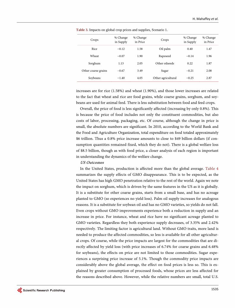
The supply price of these commodities is affected more significantly. This is an eco-nomically intuitive result. The supply price of other coarse grains (which includes corn) increases by 3.49%, and the supply price of soybeans increases by 4.05%. Table 3 sum-marizes the impact on supply and supply prices at the global level. The lowest price

H. Mahaffey et al.

1535

Table 3. Impacts on global crop prices and supplies, Scenario 1.

Crops % Change in Supply

% Change in Price

Crops % Change in Supply

% Change in Price

Rice −0.12 1.58 Oil palm 0.40 1.47

Wheat −0.07 1.90 Rapeseed −0.14 1.96

Sorghum 1.13 2.05 Other oilseeds 0.22 1.87

Other coarse grains −0.67 3.49 Sugar −0.21 2.08

Soybeans −1.40 4.05 Other agricultural −0.25 2.87

increases are for rice (1.58%) and wheat (1.90%), and those lower increases are related to the fact that wheat and rice are food grains, while coarse grains, sorghum, and soy-beans are used for animal feed. There is less substitution between food and feed crops.

Overall, the price of food is less significantly affected (increasing by only 0.8%). This is because the price of food includes not only the constituent commodities, but also costs of labor, processing, packaging, etc. Of course, although the change in price is small, the absolute numbers are significant. In 2010, according to the World Bank and the Food and Agriculture Organization, total expenditure on food totaled approximately $6 trillion. Thus a 0.8% price increase amounts to close to $49 billion dollars (if con-sumption quantities remained fixed, which they do not). There is a global welfare loss of $8.5 billion, though as with food price, a closer analysis of each region is important in understanding the dynamics of the welfare change.

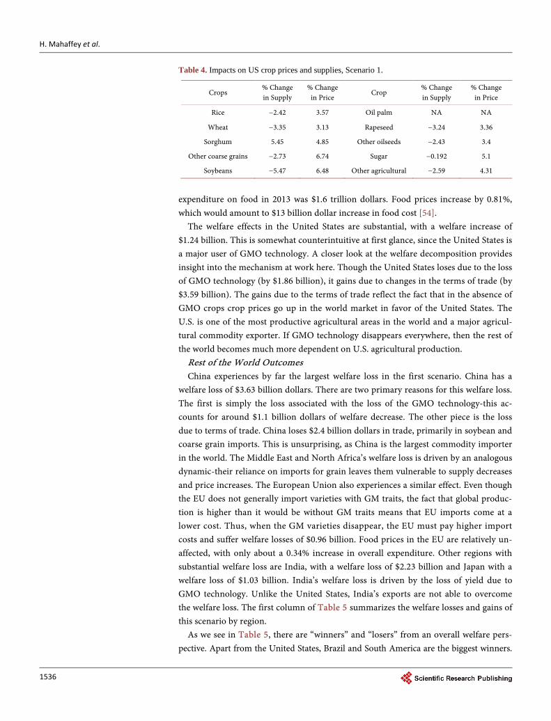
US Outcomes In the United States, production is affected more than the global average. Table 4

summarizes the supply effects of GMO disappearance. This is to be expected, as the United States has high GMO penetration relative to the rest of the world. Again we note the impact on sorghum, which is driven by the same features in the US as it is globally. It is a substitute for other coarse grains, starts from a small base, and has no acreage planted to GMO (so experiences no yield loss). Palm oil supply increases for analogous reasons. It is a substitute for soybean oil and has no GMO varieties, so yields do not fall. Even crops without GMO improvements experience both a reduction in supply and an increase in price. For instance, wheat and rice have no significant acreage planted to GMO varieties. Regardless they both experience supply decreases, of 3.35% and 2.42% respectively. The limiting factor is agricultural land. Without GMO traits, more land is needed to produce the affected commodities, so less is available for all other agricultur-al crops. Of course, while the price impacts are largest for the commodities that are di-rectly affected by yield loss (with price increases of 6.74% for coarse grains and 6.48% for soybeans), the effects on price are not limited to those commodities. Sugar expe-riences a surprising price increase of 5.1%. Though the commodity price impacts are considerably above the global average, the effect on food prices is less so. This is ex-plained by greater consumption of processed foods, whose prices are less affected for the reasons described above. However, while the relative numbers are small, total U.S.

H. Mahaffey et al.

1536

Table 4. Impacts on US crop prices and supplies, Scenario 1.

Crops % Change in Supply

% Change in Price

Crop % Change in Supply

% Change in Price

Rice −2.42 3.57 Oil palm NA NA

Wheat −3.35 3.13 Rapeseed −3.24 3.36

Sorghum 5.45 4.85 Other oilseeds −2.43 3.4

Other coarse grains −2.73 6.74 Sugar −0.192 5.1

Soybeans −5.47 6.48 Other agricultural −2.59 4.31

expenditure on food in 2013 was $1.6 trillion dollars. Food prices increase by 0.81%, which would amount to $13 billion dollar increase in food cost [54].

The welfare effects in the United States are substantial, with a welfare increase of $1.24 billion. This is somewhat counterintuitive at first glance, since the United States is a major user of GMO technology. A closer look at the welfare decomposition provides insight into the mechanism at work here. Though the United States loses due to the loss of GMO technology (by $1.86 billion), it gains due to changes in the terms of trade (by $3.59 billion). The gains due to the terms of trade reflect the fact that in the absence of GMO crops crop prices go up in the world market in favor of the United States. The U.S. is one of the most productive agricultural areas in the world and a major agricul-tural commodity exporter. If GMO technology disappears everywhere, then the rest of the world becomes much more dependent on U.S. agricultural production.

Rest of the World Outcomes China experiences by far the largest welfare loss in the first scenario. China has a

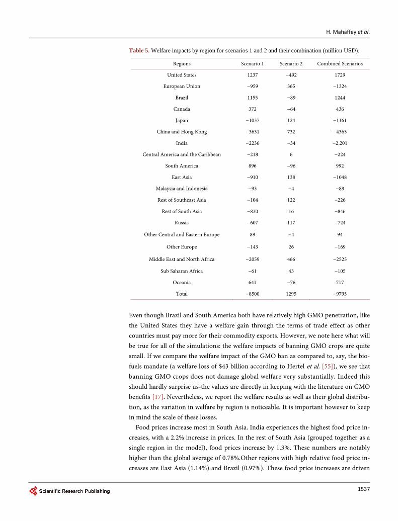
welfare loss of $3.63 billion dollars. There are two primary reasons for this welfare loss. The first is simply the loss associated with the loss of the GMO technology-this ac-counts for around $1.1 billion dollars of welfare decrease. The other piece is the loss due to terms of trade. China loses $2.4 billion dollars in trade, primarily in soybean and coarse grain imports. This is unsurprising, as China is the largest commodity importer in the world. The Middle East and North Africa’s welfare loss is driven by an analogous dynamic-their reliance on imports for grain leaves them vulnerable to supply decreases and price increases. The European Union also experiences a similar effect. Even though the EU does not generally import varieties with GM traits, the fact that global produc-tion is higher than it would be without GM traits means that EU imports come at a lower cost. Thus, when the GM varieties disappear, the EU must pay higher import costs and suffer welfare losses of $0.96 billion. Food prices in the EU are relatively un-affected, with only about a 0.34% increase in overall expenditure. Other regions with substantial welfare loss are India, with a welfare loss of $2.23 billion and Japan with a welfare loss of $1.03 billion. India’s welfare loss is driven by the loss of yield due to GMO technology. Unlike the United States, India’s exports are not able to overcome the welfare loss. The first column of Table 5 summarizes the welfare losses and gains of this scenario by region.

As we see in Table 5, there are “winners” and “losers” from an overall welfare pers-pective. Apart from the United States, Brazil and South America are the biggest winners.

H. Mahaffey et al.

1537

Table 5. Welfare impacts by region for scenarios 1 and 2 and their combination (million USD).

Regions Scenario 1 Scenario 2 Combined Scenarios

United States 1237 −492 1729

European Union −959 365 −1324

Brazil 1155 −89 1244

Canada 372 −64 436

Japan −1037 124 −1161

China and Hong Kong −3631 732 −4363

India −2236 −34 −2,201

Central America and the Caribbean −218 6 −224

South America 896 −96 992

East Asia −910 138 −1048

Malaysia and Indonesia −93 −4 −89

Rest of Southeast Asia −104 122 −226

Rest of South Asia −830 16 −846

Russia −607 117 −724

Other Central and Eastern Europe 89 −4 94

Other Europe −143 26 −169

Middle East and North Africa −2059 466 −2525

Sub Saharan Africa −61 43 −105

Oceania 641 −76 717

Total −8500 1295 −9795

Even though Brazil and South America both have relatively high GMO penetration, like the United States they have a welfare gain through the terms of trade effect as other countries must pay more for their commodity exports. However, we note here what will be true for all of the simulations: the welfare impacts of banning GMO crops are quite small. If we compare the welfare impact of the GMO ban as compared to, say, the bio-fuels mandate (a welfare loss of $43 billion according to Hertel et al. [55]), we see that banning GMO crops does not damage global welfare very substantially. Indeed this should hardly surprise us-the values are directly in keeping with the literature on GMO benefits [17]. Nevertheless, we report the welfare results as well as their global distribu-tion, as the variation in welfare by region is noticeable. It is important however to keep in mind the scale of these losses.

Food prices increase most in South Asia. India experiences the highest food price in-creases, with a 2.2% increase in prices. In the rest of South Asia (grouped together as a single region in the model), food prices increase by 1.3%. These numbers are notably higher than the global average of 0.78%.Other regions with high relative food price in-creases are East Asia (1.14%) and Brazil (0.97%). These food price increases are driven

H. Mahaffey et al.

1538

by higher consumption of raw commodities, rice in particular, and lower consumption of processed food.

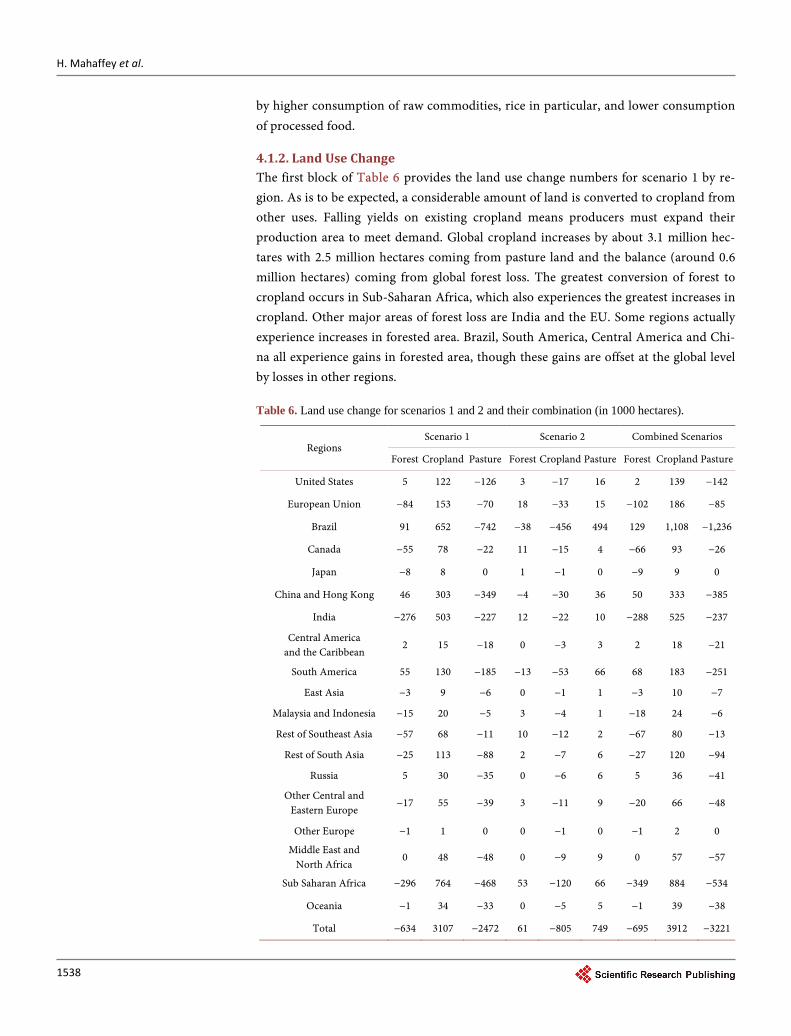
4.1.2. Land Use Change The first block of Table 6 provides the land use change numbers for scenario 1 by re-gion. As is to be expected, a considerable amount of land is converted to cropland from other uses. Falling yields on existing cropland means producers must expand their production area to meet demand. Global cropland increases by about 3.1 million hec-tares with 2.5 million hectares coming from pasture land and the balance (around 0.6 million hectares) coming from global forest loss. The greatest conversion of forest to cropland occurs in Sub-Saharan Africa, which also experiences the greatest increases in cropland. Other major areas of forest loss are India and the EU. Some regions actually experience increases in forested area. Brazil, South America, Central America and Chi-na all experience gains in forested area, though these gains are offset at the global level by losses in other regions. Table 6. Land use change for scenarios 1 and 2 and their combination (in 1000 hectares).

Regions Scenario 1 Scenario 2 Combined Scenarios

Forest Cropland Pasture Forest Cropland Pasture Forest Cropland Pasture

United States 5 122 −126 3 −17 16 2 139 −142

European Union −84 153 −70 18 −33 15 −102 186 −85

Brazil 91 652 −742 −38 −456 494 129 1,108 −1,236

Canada −55 78 −22 11 −15 4 −66 93 −26

Japan −8 8 0 1 −1 0 −9 9 0

China and Hong Kong 46 303 −349 −4 −30 36 50 333 −385

India −276 503 −227 12 −22 10 −288 525 −237

Central America and the Caribbean

2 15 −18 0 −3 3 2 18 −21

South America 55 130 −185 −13 −53 66 68 183 −251

East Asia −3 9 −6 0 −1 1 −3 10 −7

Malaysia and Indonesia −15 20 −5 3 −4 1 −18 24 −6

Rest of Southeast Asia −57 68 −11 10 −12 2 −67 80 −13

Rest of South Asia −25 113 −88 2 −7 6 −27 120 −94

Russia 5 30 −35 0 −6 6 5 36 −41

Other Central and Eastern Europe

−17 55 −39 3 −11 9 −20 66 −48

Other Europe −1 1 0 0 −1 0 −1 2 0

Middle East and North Africa

0 48 −48 0 −9 9 0 57 −57

Sub Saharan Africa −296 764 −468 53 −120 66 −349 884 −534

Oceania −1 34 −33 0 −5 5 −1 39 −38

Total −634 3107 −2472 61 −805 749 −695 3912 −3221

H. Mahaffey et al.

1539

One of the main problems with land use conversion to cropland is that when forest or pasture is converted to cropland, much of the carbon that has been sequestered over the years is released into the atmosphere. In addition, future sequestration is foregone. In the biofuels literature, this indirect or induced land use change and its associated emissions has been an important and controversial topic. Thus land use conversion to cropland has associated emissions increases. With the growing focus on greenhouse gases emissions, this is an important issue worth addressing. Fortunately, the results of the GTAP-BIO simulation allow us to calculate emissions changes associated with the land use change.

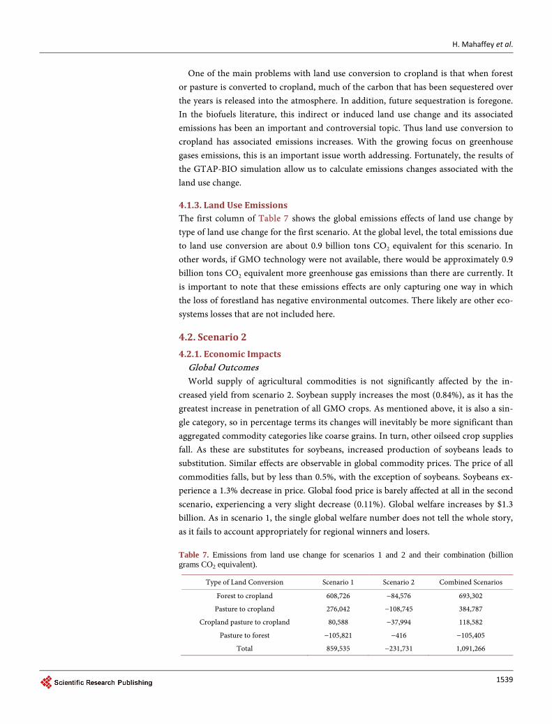
4.1.3. Land Use Emissions The first column of Table 7 shows the global emissions effects of land use change by type of land use change for the first scenario. At the global level, the total emissions due to land use conversion are about 0.9 billion tons CO2 equivalent for this scenario. In other words, if GMO technology were not available, there would be approximately 0.9 billion tons CO2 equivalent more greenhouse gas emissions than there are currently. It is important to note that these emissions effects are only capturing one way in which the loss of forestland has negative environmental outcomes. There likely are other eco-systems losses that are not included here.

4.2. Scenario 2 4.2.1. Economic Impacts

Global Outcomes World supply of agricultural commodities is not significantly affected by the in-

creased yield from scenario 2. Soybean supply increases the most (0.84%), as it has the greatest increase in penetration of all GMO crops. As mentioned above, it is also a sin-gle category, so in percentage terms its changes will inevitably be more significant than aggregated commodity categories like coarse grains. In turn, other oilseed crop supplies fall. As these are substitutes for soybeans, increased production of soybeans leads to substitution. Similar effects are observable in global commodity prices. The price of all commodities falls, but by less than 0.5%, with the exception of soybeans. Soybeans ex-perience a 1.3% decrease in price. Global food price is barely affected at all in the second scenario, experiencing a very slight decrease (0.11%). Global welfare increases by $1.3 billion. As in scenario 1, the single global welfare number does not tell the whole story, as it fails to account appropriately for regional winners and losers. Table 7. Emissions from land use change for scenarios 1 and 2 and their combination (billion grams CO2 equivalent).

Type of Land Conversion Scenario 1 Scenario 2 Combined Scenarios

Forest to cropland 608,726 −84,576 693,302

Pasture to cropland 276,042 −108,745 384,787

Cropland pasture to cropland 80,588 −37,994 118,582

Pasture to forest −105,821 −416 −105,405

Total 859,535 −231,731 1,091,266

H. Mahaffey et al.

1540

US Outcomes Unlike in scenario 1, the US experiences slight impacts relative to the rest of the

world. This is to be expected. The approach we took in modeling scenario 2 means that the United States experiences no yield improvements. Thus the production effects in the United States are negligible. Total supply of all commodities stays even or falls-most notably for soybeans, where supply falls by 1.3%. Imports from other soybean produc-ers become more affordable, thus lowering domestic production. This might not seem especially significant, but 1% of total US soybean production is close to 33 million bu-shels. Still, relative to total production, the effects are not important. Falling production and prices indicate that cheaper supply is now coming from other regions. In fact, a closer look at the terms of trade effects and the harvested area reveals that the increase in yields in the rest of the world changes to some extent the locations of agricultural production. United States producers move out of oilseed production and into wheat, rice and other coarse grains. As mentioned before, wheat and rice have little to no area planted to GMO varieties. Thus no country is gaining any advantage relative to the United States in those crops, explaining the increase.

The United States is a loser in net welfare in the second scenario. The United States experiences welfare losses of $492 million. The vast majority of those losses come from trade. As production in the rest of the world increases, the United States loses out to other exporters.

Rest of the World Outcomes As in the first scenario, China experiences the most significant welfare impacts. This

time, however, China gains $0.73 billion. The mechanism is analogous to the first sce-nario. China benefits from the rising supply (and falling price) of grains and oilseeds. In particular, the decreased price of soybeans is a particular boon to China.

Other beneficiaries are the Middle East and North Africa ($0.47 billion) and the EU ($0.37 billion). This is no surprise; just as for China, the mechanisms for loss and gain are roughly symmetrical in scenario 1 and scenario 2. Brazil and South America expe-rience the largest losses in welfare ($89.2 million and $96.5 million, respectively). There is symmetry to the results of scenario 1 and scenario 2: welfare gains in scenario 1 are matched by welfare losses in scenario 2, and vice versa. The second column of Table 5 gives the overall welfare effects by region for this scenario.

Food price effects are negligible across the world-the most significant drop in food price occurs in the Brazil (0.38%).

4.2.2. Land Use Change As global yields improve, we anticipate less area planted to crops. This is what we ob-serve in the simulation results. Global cropland decreases by about 0.8 million hectares. Forests cover 0.06 million more hectares, and pasture for livestock covers the other 0.74 million hectares currently devoted to crops. The European Union and Sub Saharan Africa experience the largest increases in forestland (0.02 million hectares and 0.53 mil-lion hectares, respectively). Though Brazil experiences the greatest decreases in crop-

H. Mahaffey et al.

1541

land (0.46 million hectares), most of that land is converted to pasture, rather than forest. The second block of Table 6 represent land use change by region for this scenario

4.2.3. Land Use Emissions As in the previous scenario, the land use conversion has emissions impacts. Since the conversion is now from cropland to other uses, the emissions impacts are negative. A counterfactual world with higher GMO penetration is a world with less GHG emissions. Simply by increasing the penetration of GMO crops in countries currently using GMO to the United States” level of penetration, greenhouse gas emissions fall by 0.2 billion tons CO2 equivalent. The second column of Table 7 summarizes the global sources of emissions decrease.

4.3. Combination of Scenarios 1 and 2 4.3.1. Economic Impacts Lastly, we consider the scenarios together. We recall that the previous results have all been understood relative to the actual world. Scenario 1 considers the world in the ab-sence of GMO technology; scenario 2 considers the world with increased GMO pene-tration. Having considered these scenarios separately, we now take them together. Here our goal is not to compare counterfactual worlds to the actual world, but rather to con-sider the future. One way of thinking about this is to consider this as an estimation of the cost of banning GMO crops. Instead of comparing the ban to the current world, which assumes that the penetration of GMO crops will remain static, we compare the outcomes in the case of a ban to the outcomes in the case of a likely future scenario. In this case, we understand scenario 2 as the plausible alternative outcome. Based on the rising penetration of GMOs worldwide, it is not unreasonable to assume that penetra-tion will reach the levels it has attained in the United States. In fact, it would not be un-reasonable to assume that GMO penetration far exceeds the penetration we model here. That being said, given the number of unknown variables, this seems a reasonable way to conservatively estimate of the future costs of a GMO ban (or the future benefits of GMOs).

In considering the scenarios relative to each other, we consider the welfare effects and land use/emissions effects. Clearly the commodity price impacts and food cost im-pacts would be higher, but it is not possible to directly combine those results.

In order to compare the welfare costs of a future GMO ban, we take the welfare re-sults from scenario 1 and subtract the welfare impacts from scenario 2. This gives the welfare impact of a GMO ban given the welfare impacts of the increased GMO penetra-tion from scenario 2. Global welfare loss is $9.8 billion. China is especially hard hit, with welfare losses accounting for more than 40% of global welfare loss. The third column of Table 5 gives the difference in welfare impact by region.

Here the winners and losers of the GMO ban are made even clearer than in either scenario taken alone. Besides China, India and the Middle East and North Africa are the hardest hit, with Brazil and the United States reaping significant rewards. Given the regulatory approaches of the various regions represented here, the results are somewhat

H. Mahaffey et al.

1542

surprising. On the whole, as GMO penetration increases in GMO using countries, a GMO ban hurts low GMO penetration regions more and more. Export heavy regions are also the regions with the most significant penetration of GMO crops. Importers in turn rely on the marginal production of these GMO using producers. When the GMO varieties disappear, it is the importers who must meet their demand with higher prices that are adversely impacted the most.

4.3.2. Land Use Change A similar procedure allows us to determine the land use effects of a future GMO ban. The third block of Table 6 summarizes the land use impacts of the future GMO ban. From the first column of this table, it is clear that much of the conversion of forest to crop is occurring in either the developing world or in places with at-risk forests to be-gin with. Sub Saharan Africa has the largest forest loss, losing about 0.3 million hectares of forest. India also loses significant forested area (also around 0.3 million hectares).

4.3.3. Land USE Emissions The global emissions outcomes combining scenario 2 and scenario 1 is approximately 1.1 billion tons of CO2 equivalent (see the last column of Table 7). It is clear from these results that GMOs are a significant factor in the “greening” of agriculture. After energy production, agriculture is the largest source of greenhouse gas emissions. This level of emissions is about three times the land use change emissions from the entire US etha-nol program. The emission reduction impact of GMO varieties is rarely mentioned in the GMO debate.

5. Conclusions

The objective of this paper was to quantify the economic and environmental impacts of banning GMO crops. Using a well-known CGE model (GTAP-BIO), two counterfac-tual scenarios were examined to reach these goals. The first is a GMO ban, while the second is an increase in total GMO penetration. The economic impacts include welfare, price, and supply impacts. The environmental impacts focus on land use change and associated emissions change.

As GMO finds wider and wider usage, there is a corresponding growth in the popu-lar hysteria surrounding the technology. Environmental activists push for GMO bans, without adequately considering the impacts such bans might have. The losses asso-ciated with a global ban would be twofold: the losses actually realized and the potential losses when compared to an alternative adoption schema. These losses are also not merely economic. To frame the debate as environmentalists on one side, and capitalists (and purveyors of capitalist apologetics) on the other, a more complex issue is oversim-plified. There are environmental gains associated with GMO technology, and while the welfare effects of GMO technology are not, as it turns out, especially substantial at the global level, the environmental effects are. Both sides of the GMO debate are done a disservice if these effects are ignored.

While the welfare impacts are not substantial at the global level, there are economic

H. Mahaffey et al.

1543

effects worth noting. In particular, the supply price and food price increases are ex-tremely region specific. While the United States does not even experience a 1% food increase, countries like India and other South Asian nations do see their food prices in-crease more noticeably (2.2% and 1.3%). These are parts of the world where food and beverage expenditure is already a greater share of total household consumption, and so the effect of the food price increase is in fact amplified. It is a luxury to be relatively un-affected by a GMO ban, or at least to have your pocketbook hit less hard. Interestingly, the welfare and supply effects suggest that in the case of a GMO ban, the world be-comes more dependent on US agriculture. This might not be a desirable outcome for nations other than the United States. Indeed, the United States is the country that bene-fits most from a GMO ban, either present or future.

The welfare impacts are in line with the impacts estimated in the rest of the literature [17]. Because they are the results of a global GMO ban of all three main crops, they are slightly greater than studies which have focused on one region, or one crop’s benefits. However, the overall economic impacts of GMO crops have been discussed at great length, both at the micro and macro level.

What have been more sparsely covered in the literature are the land use change im-pacts. Indeed Barrows et al. [56] in their examination on land use change and GMO point to the need for a full general equilibrium analysis to assess the impacts of land use change on price, supply but also on greenhouse gas emissions. Our findings suggest that avoided land use change (and thus avoided increases in emissions) is one of the most important benefits associated with GMO technology. Following the completion of the latest talks in Paris, countries have expressed a willingness to lower overall emis-sions, and GMO technology is one of the ways that agriculture can help this aim. Agri-culture would have to find alternative approaches to lowering emissions, and these are not immediately obvious without fundamentally altering the agricultural landscape (e.g. banning meat).

This work is among the first to use the updated 2011 data from GTAP. Thus it is run using the most recent global economic information. Undertaking to model, a global GMO ban requires that global data be used, and preferably the best global data availa-ble—this allows this work to provide a fuller picture of the world impacts.

References [1] United States Department of Agriculture (2016) Glossary of Agricultural Biotechnology

Terms. http://www.usda.gov/wps/portal/usda/usdahome?navid=BIOTECH_GLOSS&navtype=RT&parentnav=BIOTECH

[2] Taleb, N., et al. (2014) The Precautionary Principle (with Application to the Genetic Mod-ification of Organisms). Extreme Risk Initiative—NYU School of Engineering Working Paper Series.

[3] Dawkins, R. (1998) Where Do the Real Dangers of Genetic Engineering Lie? London Even-ing Standard, London.

[4] Singer, P.A. and Daar, A.S. (2000) Avoiding Frankendrugs. Nature Biotechnology, 18, 1225.

H. Mahaffey et al.

1544

http://dx.doi.org/10.1038/82256

[5] Fernandez-Cornejo, J., Wechsler, S.J., Livingston, M. and Mitchell, L. (2014) Genetically Engineered Crops in the United States. Economic Research Report No. (ERR-162), 60 p.

[6] Lusk, J.L., et al. (2005) A Meta-Analysis of Genetically Modified Food Valuation Studies. Journal of Agricultural and Resource Economics, 30, 28-44.

[7] Chiang, F.-S.F., Chern, W.S. and Lu, L.-J. (2005) Public Communication: Consumer’s Perspective of Gmo/Gm Foods. APO Study Meeting on Use and Regulation of Genetically Modified Organisms, China, 18-23 November 2002, 42-51.

[8] Costa-Font, J. and Mossialos, E. (2005) Is Dread of Genetically Modified Food Associated with the Consumers’ Demand for Information? Applied Economics Letters, 12, 859-863. http://dx.doi.org/10.1080/13504850500365830

[9] Costa-Font, M. and Gil, J.M. (2009) Structural Equation Modelling of Consumer Accep-tance of Genetically Modified (GM) Food in the Mediterranean Europe: A Cross Country Study. Food Quality and Preference, 20, 399-409. http://dx.doi.org/10.1016/j.foodqual.2009.02.011

[10] Shuping, N., Wong, F. and Polansek, T. (2014) China Approves Imports of GMO Syngenta corn, Pioneer Soy.

[11] EUDGARD (2007) Economic Impact of Unapproved GMOs on EU Feed Imports and Li-vestock Production. EUDGARD, Brussels.

[12] James, C. (2014) Global Status of Commercialized Biotech/GM Crops. International Service for the Acquisition of Agri-Biotech Applications (ISAAA), Ithaca.

[13] Fish, A. and Rudenko, L. (2001) Guide to US Regulation of Genetically Modified Food and Agricultural Biotechnology Products. Pew Initiative on Food and Biotechnology, Pew Trusts.

[14] Hemphill, T.A. and Banerjee, S. (2015) Genetically Modified Organisms and the US Retail Food Labeling Controversy: Consumer Perceptions, Regulation, and Public Policy. Business and Society Review, 120, 435-464. http://dx.doi.org/10.1111/basr.12062

[15] Brookes, G. and Barfoot, P. (2015) GM Crops: Global Socio-Economic and Environmental Impacts 1996-2013. PG Economics Ltd., Dorchester.

[16] Brookes, G. and Barfoot, P. (2012) The Income and Production Effects of Biotech Crops Globally 1996-2010. GM Crops Food, 3, 265-272. http://dx.doi.org/10.4161/gmcr.20097

[17] Qaim, M. (2009) The Economics of Genetically Modified Crops. Annual Review of Re-source Economics, 1, 665-694. http://dx.doi.org/10.1146/annurev.resource.050708.144203

[18] Brookes, G. and Barfoot, P. (2015) Global Income and Production Impacts of Using GM Crop Technology 1996-2013. GM Crops & Food, 6, 13-46. http://dx.doi.org/10.1080/21645698.2015.1022310

[19] Lichtenberg, E. and Zilberman, D. (1986) The Econometrics of Damage Control: Why Spe-cification Matters. American Journal of Agricultural Economics, 68, 261-273. http://dx.doi.org/10.2307/1241427

[20] Piggott, N. and Marra, M. (2007) The Net Gain to Cotton Farmers of a Natural Refuge Plan for BollgardII® Cotton. AgBioForum, 10, 1-10.

[21] Nolan, E. and Santos, P. (2012) The Contribution of Genetic Modification to Changes in Corn Yield in the United States. American Journal of Agricultural Economics, 94, 1171- 1188. http://dx.doi.org/10.1093/ajae/aas069

[22] Shryock, J.J. (2013) The Economic and Performance Impact of Technology Adoption. Uni-versity of Missouri, Columbia.

H. Mahaffey et al.

1545

[23] Mutuc, M.E., Rejesus, R.M. and Yorobe Jr., J.M. (2011) Yields, Insecticide Productivity, and Bt Corn: Evidence from Damage Abatement Models in the Philippines.

[24] Burachik, M. (2010) Experience from use of GMOs in Argentinian Agriculture, Economy and Environment. New Biotechnology, 27, 588-592. http://dx.doi.org/10.1016/j.nbt.2010.05.011

[25] Huesing, J. and English, L. (2004) The Impact of Bt Crops on the Developing World.

[26] Venus, T., et al. (2011) Comparison of Bt and Non-Bt Maize Cultivation Gross Margin: A Case Study of Maize Producers from Italy, Spain and Germany. Futuragra, Rome.

[27] Kruger, M., Van Rensburg, J.B.J. and Van den Berg, J. (2009) Perspective on the Develop-ment of Stem Borer Resistance to Bt Maize and Refuge Compliance at the Vaalharts Irriga-tion Scheme in South Africa. Crop Protection, 28, 684-689. http://dx.doi.org/10.1016/j.cropro.2009.04.001

[28] Marra, M.C., Pardey, P.G. and Alston, J.M. (2002) The Payoffs to Agricultural Biotechnol-ogy: An Assessment of the Evidence. International Food Policy Research Institute, Wash-ington.

[29] Trigo, E.J. and Cap, E. (2006) Ten Years of Genetically Modified Crops in Argentine Agri-culture.

[30] Smale, M., et al. (2012) A Case of Resistance: Herbicide-Tolerant Soybeans in Bolivia.

[31] Verhalen, L., Greenhagen, B. and Thacker, R.W. (2003) Lint Yield, Lint Percentage, and Fi-ber Quality Response in Bollgard, Roundup Ready, and Bollgard/Roundup Ready Cotton. Journal of Cotton Science, 7, 23-38.

[32] Sankula, S. (2006) Crop Biotechnology in the United States: Experiences and Impacts. In: Halford, N., Ed., Plant Biotechnology: Current and Future Applications of Genetically Mod-ified Crops, Wiley, Hoboken, 28-52. http://dx.doi.org/10.1002/0470021837.ch2

[33] ICAC (2003) Bollgard II: A New Generation of Bt Genes Commercialized. International Cotton Advisory Committee.

[34] Qaim, M. and De Janvry, A. (2005) Bt Cotton and Pesticide Use in Argentina: Economic and Environmental Effects. Environment and Development Economics, 10, 179-200. http://dx.doi.org/10.1017/S1355770X04001883

[35] Tripp, R. (2009) Biotechnology and Agricultural Development: Transgenic Cotton, Rural Institutions and Resource-Poor Farmers. Routledge, Cornwall.

[36] Traxler, G. and Godoy-Avila, S. (2004) Transgenic Cotton in Mexico. AgBioForum, 7, 57- 62.

[37] Gouse, M., Pray, C. and Schimmelpfennig, D. (2005) The Distribution of Benefits from Bt Cotton Adoption in South Africa.

[38] Bennett, R., Morse, S. and Ismael, Y. (2006) The Economic Impact of Genetically Modified Cotton on South African Smallholders: Yield, Profit and Health Effects. The Journal of De-velopment Studies, 42, 662-677. http://dx.doi.org/10.1080/00220380600682215

[39] Qiao, F. (2015) Fifteen Years of Bt Cotton in China: The Economic Impact and Its Dynam-ics. World Development, 70, 177-185. http://dx.doi.org/10.1016/j.worlddev.2015.01.011

[40] Huang, J., Hu, R., Rozelle, S., Qiao, F. and Pray, C.E. (2002) Transgenic Varieties and Productivity of Smallholder Cotton Farmers in China. Australian Journal of Agricultural and Resource Economics, 46, 367-387. http://dx.doi.org/10.1111/1467-8489.00184

[41] Subramanian, A. and Qaim, M. (2010) The Impact of Bt Cotton on Poor Households in Rural India. The Journal of Development Studies, 46, 295-311.

H. Mahaffey et al.

1546

http://dx.doi.org/10.1080/00220380903002954

[42] Gandhi, V.P. and Namboodiri, N. (2006) The Adoption and Economics of Bt Cotton in In-dia: Preliminary Results from a Study.

[43] Pemsl, D., Waibel, H. and Orphal, J. (2004) A Methodology to Assess the Profitability of Bt- Cotton: Case Study Results from the State of Karnataka, India. Crop Protection, 23, 1249- 1257. http://dx.doi.org/10.1016/j.cropro.2004.05.011

[44] Ali, A. and Abdulai, A. (2010) The Adoption of Genetically Modified Cotton and Poverty Reduction in Pakistan. Journal of Agricultural Economics, 61, 175-192. http://dx.doi.org/10.1111/j.1477-9552.2009.00227.x

[45] Hertel, T.W. (1997) Global Trade Analysis: Modeling and Applications. Cambridge Uni-versity Press, Cambridge.

[46] Lee, H.-L., et al. (2005) Towards an Integrated Land Use Data Base for Assessing the Poten-tial for Greenhouse Gas Mitigation. GTAP Technical Papers, 26.

[47] Taheripour, F., et al. (2007) Introducing Liquid Biofuels into the GTAP Database. GTAP Research Memorandum. Center for Global Trade Analysis, Purdue University, West La-fayette.

[48] Hertel, T.W., et al. (2010) Effects of US Maize Ethanol on Global Land Use and Greenhouse Gas Emissions: Estimating Market-Mediated Responses. BioScience, 60, 223-231. http://dx.doi.org/10.1525/bio.2010.60.3.8

[49] Taheripour, F., Hertel, T.W. and Tyner, W.E. (2011) Implications of Biofuels Mandates for the Global Livestock Industry: A Computable General Equilibrium Analysis. Agricultural Economics, 42, 325-342. http://dx.doi.org/10.1111/j.1574-0862.2010.00517.x

[50] Liu, J., Hertel, T.W., Taheripour, F., Zhu, T. and Ringler, C. (2014) International Trade Buffers the Impact of Future Irrigation Shortfalls. Global Environmental Change, 29, 22-31. http://dx.doi.org/10.1016/j.gloenvcha.2014.07.010

[51] Taheripour, F. and Tyner, W.E. (2013) Biofuels and Land Use Change: Applying Recent Evidence to Model Estimates. Applied Sciences, 3, 14-38. http://dx.doi.org/10.3390/app3010014

[52] Qaim, M. and Zilberman, D. (2003) Yield Effects of Genetically Modified Crops in Devel-oping Countries. Science, 299, 900-902. http://dx.doi.org/10.1126/science.1080609

[53] Searchinger, T., Edwards, R., Mulligan, D., Heimlich, R. and Plevin, R. (2015) Do Biofuel Policies Seek to Cut Emissions by Cutting Food? Science, 347, 1420-1422. http://dx.doi.org/10.1126/science.1261221

[54] ERS (2014) Food and Alcoholic Beverages: Total Expenditure. http://www.ers.usda.gov/data-products/food-expenditures.aspx

[55] Hertel, T.W., Tyner, W.E. and Birur, D.K. (2010) The Global Impacts of Biofuel Mandates. Energy Journal, 31, 75-100. http://dx.doi.org/10.5547/ISSN0195-6574-EJ-Vol31-No1-4

[56] Barrows, G., Sexton, S. and Zilberman, D. (2014) The Impact of Agricultural Biotechnology on Supply and Land-Use. Environment and Development Economics, 19, 676-703. http://dx.doi.org/10.1017/S1355770X14000400

Submit or recommend next manuscript to SCIRP and we will provide best service for you:

Accepting pre-submission inquiries through Email, Facebook, LinkedIn, Twitter, etc. A wide selection of journals (inclusive of 9 subjects, more than 200 journals) Providing 24-hour high-quality service User-friendly online submission system Fair and swift peer-review system Efficient typesetting and proofreading procedure Display of the result of downloads and visits, as well as the number of cited articles Maximum dissemination of your research work

Submit your manuscript at: http://papersubmission.scirp.org/ Or contact jep@scirp.org