Evaluating the Impact of Performance- related Pay for Teachers in

THE CENTRE FOR MARKET AND PUBLIC ORGANISATION

The Centre for Market and Public Organisation, a Research Centre based at the University of Bristol, was established in 1998. The principal aim of the CMPO is to develop understanding of the design of activities within the public sector, on the boundary of the state and within recently privatised entities with the objective of developing research in, and assessing and informing policy toward, these activities.

Centre for Market and Public Organisation University of Bristol

Department of Economics Mary Paley Building

12 Priory Road Bristol BS8 1TN Tel: (0117) 954 6943

Fax: (0117) 954 6997 E-mail: [email protected]

Evaluating the Impact of Performance-related Pay for Teachers in England

Adele Atkinson, Simon Burgess, Bronwyn Croxson, Paul Gregg, Carol Propper, Helen

Slater and Deborah Wilson

December 2004

Working Paper No. 04/113

ISSN 1473-625X

CMPO Working Paper Series No. 04/113

CMPO is jointly funded by the Leverhulme Trust and the ESRC

Evaluating the Impact of Performance-related Pay for Teachers in England

Adele Atkinson1 Simon Burgess2

Bronwyn Croxson3 Paul Gregg2

Carol Propper2 Helen Slater2

Deborah Wilson2

1 Personal Finance Research Centre, University of Bristol 2 Leverhulme Centre for Market and Public Organisation, University of Bristol

3 Treasury, New Zealand.

December 2004

Abstract This paper evaluates the impact of a performance-related pay scheme for teachers in England. Using teacher level data, matched with test scores and value-added, we test whether the introduction of a payment scheme based on pupil attainment increased teacher effort. Our evaluation design controls for pupil effects, school effects and teacher effects, and adopts a difference-in-difference methodology. We find that the scheme did improve test scores and value added, on average by about half a grade per pupil. We also find heterogeneity across subjects, with maths teachers showing no improvement. Keywords: Incentives, teachers pay, education reform, pupil attainment JEL Classification: J33, J45, D23, I28

Acknowledgements The authors are grateful to the Leverhulme Trust for funding this project through CMPO. Thanks also to the Headteachers and school administrators who were very helpful in providing us with data. We are also grateful for advice from officials in the Department for Education and Skills. Finally, we thank seminar participants in Amsterdam and Bristol, plus Iwan Baranky, Marisa Ratto and Emma Tominey for useful comments. None of these are responsible for the views expressed in the paper. Address for Correspondence Department of Economics University of Bristol 12 Priory Road Bristol BS8 1TN [email protected]

1

1 Introduction

Improving education outcomes is a key priority for governments around the

world. The accumulating evidence suggests poor returns from simply raising school

resources 1, so attention has turned to other mechanisms such as school choice, and

incentives for teachers. Hanushek (2003) highlights these: “The alternative set of

potential policies emphasizes performance incentives.” (p. F93), but goes on to note that

there is very little robust evidence yet on the impact of such incentives (p. F94). In this

paper we start to plug that gap. In 1999, the UK government introduced a performance-

related pay policy for teachers, with pupil progress (value -added) as one of its key

criteria. Using longitudinal teacher-level data and a difference-in-difference research

design, we provide a quantitative evaluation of the policy’s impact on test score gains.

The incentive scheme was explicitly teacher-based (rather than school-based) and

so equivalent data is required to properly evaluate it. We have collected longitudinal data

following teachers over two complete two-year teaching cycles, before and after the

policy was introduced. By dealing with schools directly we were able to link pupils to the

teachers who taught them for specific subjects, and not rely on school level averages.

This is a crucial attribute of our data: school averages would not allow us to directly

compare the performance of eligible and ineligible teachers. For the pupils linked to the

sample teachers, we collected prior attainment data, so we can control for pupil

characteristics and measure the target of the scheme – pupil progress. Thus in the analysis

we can control for pupil and teacher fixed effects.

1 See Hanushek (2003).

2

We find important effects of the incentive scheme, that are both statistically and

economically significant. We find that teachers eligible for the incentive payment

increased their value-added by almost half a GCSE grade per pupil relative to ineligible

teachers, equal to 73% of a standard deviation. GCSE exams, taken at age 16, are the key

qualifications for entry into higher education, so these are high stakes tests and this

increase is not trivial. We find significant differences between subjects, with eligible

maths teachers showing no effect of the scheme.

Our difference-in-difference research design means that differences in general

between eligible and ineligible teachers drop out once comparisons are made over time.

We compute the change in each teacher’s average test score gain between two complete

teaching cycles, and compare the results for eligible and ineligible teachers. In the

scheme, the chance to earn the initial performance bonus was offered to teachers who had

been in the profession for about 8 years. Thus eligible and ineligible teachers differed

systematically in experience, and such differences in experience will not drop out of the

difference-in-difference if there is a non-linear experience-effectiveness relationship.

Specifically, if teachers improve in their capacity to generate value -added but at a

decreasing rate, then all else equal we would see greater improvements in progress

between the two teaching cycles for the less experienced (ineligible) group. Therefore we

also perform regression analysis, controlling for teacher experience, detailed in section 6.

The rest of the paper is organized as follows. The next section reviews the

literature on incentive schemes for teachers. Section 3 discusses the UK scheme and

section 4 our evaluation methodology. Section 5 describes the data and section 6 presents

the results. Finally, section 7 offers some conclusions.

3

2 Previous literature

There is a large literature on the effects of incentives in the private sector (see

Prendergast (1999) and Murphy (1999) for surveys). There is a smaller but growing body

of evidence about incentives in the public sector (see surveys by Dixit (2002) and

Burgess and Ratto (2003)). Some recent empirical work has produced convincing results

suggesting that incentives do affect the behaviour of employees in particular parts of the

public sector (see, for example, Courty and Marschke (2001) and Kahn, Silva and Ziliak

(2001)).

There is some quantitative evidence on the effects of teacher incentive schemes

on pupil attainment. The literature has been hampered by difficulties in finding

measurable proxies for key variables, in obtaining individual-level data, and in designing

evaluations which include adequate controls when incentive schemes are not introduced

as part of an experimental design. Lazear (2003) sets out a theoretical framework for

thinking about performance-related pay (PRP) for teachers. He discusses the pros and

cons of PRP in general, and then as applied to the case of teachers. PRP plays two roles –

an incentive mechanism to elicit greater effort, and a recruitment and retention device to

improve average teacher quality. Our study focuses on the former, and we briefly review

previous findings on this issue.

Early studies by Ladd (1999), by Cooper and Cohn (1997) and by Boozer (1999)

found a positive relationship between incentive schemes and pupil attainment, however

the results of these studies are not conclusive. Ladd (1999) compared gains in school-

level test scores in Dallas with gains in other cities, to evaluate the impact of a school-

4

level bonus scheme introduced in Dallas. The study is limited by the lack of data enabling

“before/after” comparisons, or controls for pupil, teacher or school fixed effects, however

Ladd is able to control for a number of school characteristics, such as racial mix and

relative deprivation. The results are generally positive, in that pass rates appeared to

increase faster in Dallas than in other cities. Effects differ by ethnic sub-groups, being

most positive for Hispanics and whites, and insignificant for blacks. The results are,

however, muddied by the fact that a positive Dallas effect is also found for the year

before the scheme was introduced.

Cooper and Cohn (1997) and Boozer (1999) evaluate a South Carolina scheme,

which included both school-level rewards and rewards to individual teachers. Pupil

effects are controlled for, since the dependent variables are gain in median class test

scores, and the studies also control for teacher characteristics and for class-level pupil

characteristics. The incentive plan variables were positive and significant. However this

variable confounds both incentive effects and selection effects, since teachers could

choose whether or not to apply for an award. As Cooper and Cohn put it, “It is possible,

even likely, that only the most productive teachers choose to apply for an award”

(pp.320-1).

Studies by Eberts et al.(2000), by Figlio and Kenny (2003) and by Dee and Keys

(2004) were able to use rich data sets to control for many potentially confounding

variables. It is, however, notable that although these papers assess the relationship

between incentive schemes and pupil attainment, they evaluate schemes which did not

directly link rewards to pupil attainment. Promotion was based on overall good

performance, which included time spent in the classroom, evidence of skills and

5

classroom evaluation; test results were not the major deciding factor in measuring

‘success’. Eberts et al (2000) used difference-in-difference techniques to assess the

impact on pupil attainment of a Michigan merit pay scheme which rewarded individual

teachers according to student retention rates and their performance on pupil evaluation

questionnaires. The scheme did not directly target pupil attainment although it was hoped

that this would be an indirect benefit of the scheme. The scheme had a positive and

significant impact on student retention. However, pass rates decreased, and attendance

rates and grade point averages were unchanged. The authors conclude “that incentive

systems within complex organisations such as schools,…may produce results that are

unintended and at times misdirected.” (p.19).

Figlio and Kenny (2003) combine panel data from the US National Education

Longitudinal Survey to estimate the effects of teacher incentives on an education

production function. They define incentive schemes as any merit raise or bonus awarded

to any proportion of teachers in a school. The variables do not identify whether schemes

intended rewards to be tied directly to pupil attainment. They control for various student,

teacher, school and family characteristics. The results are positive, particularly in public

and poor schools. Test scores are higher in schemes that are more high powered, in the

sense of being given to only small numbers of teachers within a school and offering

higher rewards. However, the results may not be generalisable since the schools that

responded to the survey are not representative of schools in the US.

Dee and Keys (2004) use a fixed effects model to estimate incentive effects on

student SAT scores in the Tennessee STAR and Career Ladder Evaluation schemes. The

contemporaneous data from STAR reduces the problem of unobserved heterogeneity in

6

student propensity for achievement. There are controls for pupil, teacher and class fixed

effects and characteristics. The results show a positive effect, which varies across

subjects and with teacher seniority. The authors investigated whether the results were

biased by the high rate of student attrition from the schools participating in STAR by

imputing test scores for those students who left, but the results remained similar.

Studies from Kenya and from Israel have been able to capitalize on the

experimental design of incentive schemes and use difference-in-difference techniques to

control for confounding variables. Glewwe, Ilias and Kremer (2003) investigate a Kenyan

school-based incentive scheme, by comparing differences in test scores between

treatment and comparison schools. Differences in test scores are positive and significant

in the scheme’s second year in both the random effects and difference-in-difference

models.

In a series of papers, Lavy analyses the impact of incentive schemes introduced in

Israel: two school-level schemes targeted on a variety of outcomes (Lavy 2001); and a

tournament scheme which rewarded individual teachers according to their pupils’

attainment (Lavy 2003, 2004). In the first paper, evaluating the school-level scheme, the

quasi-experimental design of the scheme allowed Lavy to employ difference in difference

techniques and control for school fixed effects. Results on all student outcomes are

positive. The schemes include both financial and non-financial rewards: Lavy compares

their cost effectiveness and concludes that money incentives are the more effective, but

that the schools included in the scheme are probably not representative of all Israeli

schools. Lavy (2003, 2004) uses panel data to evaluate the effects of a teacher-based

tournament scheme on pupil attainment. A rich dataset allowed for propensity score

7

matching and OLS estimates to be calculated, controlling for various student (including

lagged) characteristics and school covariates. The results are positive and significantly

different from zero, but are complicated by non random assignment to the program.

However, identification strategies based on a regression discontinuity design and

particularly matching, produce similar results, suggesting that there was indeed a positive

relationship between the incentive scheme and pupil test scores. The results of a follow

up survey suggest that the results were achieved by reducing class size and increased

teacher effort. Again, however, Lavy suggests that the schools may not be a

representative sample of Israeli schools.

In summary, the results of the earlier literature in this area are confounded by the

problems of distinguishing the effects of teacher quality from the effects of increased

teacher effort, and by the problems of controlling for other fixed effects such as pupil

ability. Later studies which have been able to use rich data sets to manage identifications

problems have found a positive relationship between financial incentives and pupil

attainment. Most studies, including our own, work on an un-representative sample of

schools.

3 The English education sector and the PRP scheme

(a) The structure of the English education market

The English education system has been choice-based since the Education Reform Act of

1988, which introduced a ‘quasi-market’ in education (Glennerster 1991). The following

key features of the education quasi-market remain to the present date: some degree of

8

parental choice on schools, with money following the pupils; funding and management of

schools devolved to a more local level, but with funding provided by central government,

out of general taxation revenue. The intention was that per capita funding and parental

choice would bring about competition between schools for pupils, which would raise

educational outcomes. While the quasi-market increased the autonomy of individual

schools, each school still operates within a fairly centralised system. Central government

regulates the way in which the quasi-market can operate, as well as controlling the

contents of the national curriculum and the accompanying set of national exams (detailed

more below). Pay scales for teachers are also centrally determined.

Parental choice is informed by a range of indicators for each school. The “league

tables” report the results of exams taken by all pupils at the end of each Key Stage of the

national curriculum; at ages 7, 11 (taken in primary school), 14 and 16 (taken in

secondary school). These tests are known respectively as Key Stage 1 (KS1) to Key Stage

4 (KS4) exams. Pupils take KS1, KS2 and KS3 tests in English, maths and science. KS4

exams, taken at the end of compulsory schooling, cover a much broader mix of subjects,

and comprise two different types of exam known as GCSE and GNVQ, the latter

historically being associated with more vocational subjects. English, maths and science

are compulsory for all students at KS4 as GCSE exams, in addition to which they are able

to choose from a broad range of options. For secondary schools (our focus in this paper)

the primary focus of both schools and parents has been the raw output indicator of the

proportion of pupils gaining five or more KS4 passes between grades A * and C. In this

paper, we consider teacher impact on both raw output – GCSE grades – and on value

9

added, i.e. test score gains between KS3 and GCSE. In all our analyses, we focus on the

compulsory subjects of English, maths and science to eliminate selection effects.

(b) The PRP scheme

Interest in PRP grew during the 1980s, stimulated by a perception that teaching

standards were poor and contributing to low educational attainment and, perhaps, to poor

economic performance (Tomlinson 1992, 2000)2. During the 1990s, successive

administrations attempted to introduce some form of PRP into state schools, but

succeeded only in introducing PRP for headteachers and their deputies (Marsden and

French 1998).

The 1997 Labour administration signalled a range of reforms to education in a

consultative Government paper published in 1998: “Teachers: meeting the challenge of

change”. The reforms included the introduction of a performance-related system, the

Performance Threshold plus the Upper Pay Scale, designed to affect teacher effort as well

as recruitment into and retention within the profession. The Green Paper argued that

teacher motivation was adversely affected by a culture which did not recognise and

reward outstanding performance. The scheme was introduced in the academic year

1999/2000, with the first applications submitted by teachers in July 2000.

Prior to the introduction of the PRP scheme, all teachers were paid on a unified

basic salary scale, which had nine full points, ranging from £14,658 – £23,193 per annum

(2000 prices). An individual’s position on the scale depended on his/her qualifications

2 Performance related pay for teachers is not a new idea. During the second half of the nineteenth century teachers in English state secondary schools were paid according to students’ exam results, but this was abandoned because it was believed to reward teachers who concentrated on more able pupils (Hood et al 1999). Formal systems of performance related pay (PRP) were not used in state schools during most of the twentieth century.

10

and experience, and teachers usually progressed up the scale in annual increments. In

addition to the basic salary, there were management, excellence, or recruitment and

retention points (School Teachers’ Review Body 2000). In 1999/2000, about 75% of

teachers were at the top of this scale, at spine point 9.

After the reforms, teachers at spine point 9 could apply to pass the Performance

Threshold. Passing the Threshold has two effects. First, it gives teachers an annual bonus

of £2,000, payable without revision until the end of their career and included in

calculations of pensionable salary. It is therefore of significant lifetime value. Second,

once over the Threshold, teachers move onto a new Upper Pay Scale (UPS), which

comprises additional increments, each of which are also related to performance 3.

To pass the Threshold, individual teachers had to demonstrate that they had

reached acceptable standards in five areas: knowledge and understanding of teaching;

teaching management and assessment; wider professional effectiveness; professional

characteristics; and pupil progress (DfEE 2000). In the area of pupil progress, the focus

of our evaluation, the Threshold application form gave teachers the following instruction:

“Please summarise evidence that as a result of your teaching your pupils achieve

well relative to their prior attainment, making progress as good or better than

similar pupils nationally. This should be shown in marks or grades in any

relevant national tests or examinations, or school based assessment for pupils

where national tests and examinations are not taken” (DfEE 2000).

3 In 2000 the UPS comprised five spine points; this has since been reduced to three (www.teachernet.gov.uk provides more information).

11

Teachers were required to complete their application forms by July 2000,

demonstrating their performance in each of the five areas. The information provided did

not necessarily just cover the year 1999/2000 but could be based on the teacher’s career

to that point. Passing the Threshold was largely about rewarding historical performance,

and so cannot be considered true performance pay. However, passing did give access to

the Upper Pay Scale which does offer conventional pay performance pay.

80 per cent of eligible teachers applied. Headteachers then assessed each

application and recommended whether or not individual teacher s should pass the

Threshold. Each school was then audited by an external assessor. Teachers who didn’t

pass had limited rights of appeal. Performance Threshold payments were funded out of a

separate budget, administered by central government, with no limit or quota on the

number of teachers allowed to obtain these payments4.

Progressing up the UPS was similarly focussed on “sustained and substantial

performance”, and Headteachers were required to conduct a performance review before

awarding a pay increase.

Wragg et al (2001) conducted a survey of a random sample of 1000 schools in

order to investigate this process. They found that in these schools, 88 percent of the

eligible teachers applied, and of these, 97 percent were awarded the bonus. This very high

figure influences the interpretation of the scheme. It suggests that, ex post, the initial

Threshold operated more as a general pay increase for (almost) all teachers at the eligible

point of the scale. Clearly, an unconditional pay increase will have little impact on

4 See Croxson and Atkinson (2001a, b) for an analysis of headteachers’ views on both the implementation and the impact of the Performance Threshold.

12

teacher effort, though it may help staff retention rates. In fact, evidence from Marsden

(2000) suggests that ex ante it was seen by a majority of teachers as a real incentive

scheme, and not as a general pay rise. Marsden (2000) reports on his survey of teachers

taken after the Performance Threshold was announced, but before it was implemented.

Two particular questions on the questionnaire are relevant to us:

Disagree (%)

Neutral (%)

Agree (%)

“The Green Paper pay system is a device to avoid paying more money to all teachers”

9 18 68

“In practice, many excellent teachers will not pass the Threshold because there is certain to be a quota on places available”

3 8 82

Source, Marsden. D (2000), p. 4 Sample size is c. 3000.

This suggests that a substantial majority of teachers were expecting the scheme to

be ‘real’ – that is, for only some teachers to be awarded the bonus. Given this, we should

expect to see an impact on effort for eligible teachers. This impact should be reinforced

by the forward-looking element of the scheme, the Upper Pay Scale, progress up which is

dependent on additional assessments of individual teacher performance.

4 Evaluation Methodology

In this section we set out the model and evaluation methodology. Pupils are

indexed i, teachers j, and teaching cycle (data tranche) t. Denote the pupil’s test score by

g, value added by v, pupil ability by Z and pupil effort by e. Teacher effectiveness is X,

performance pay eligibility is I, and experience is W. School effects on test scores are

denoted S , a common time effect is T (for example, due to changes in testing) and test

13

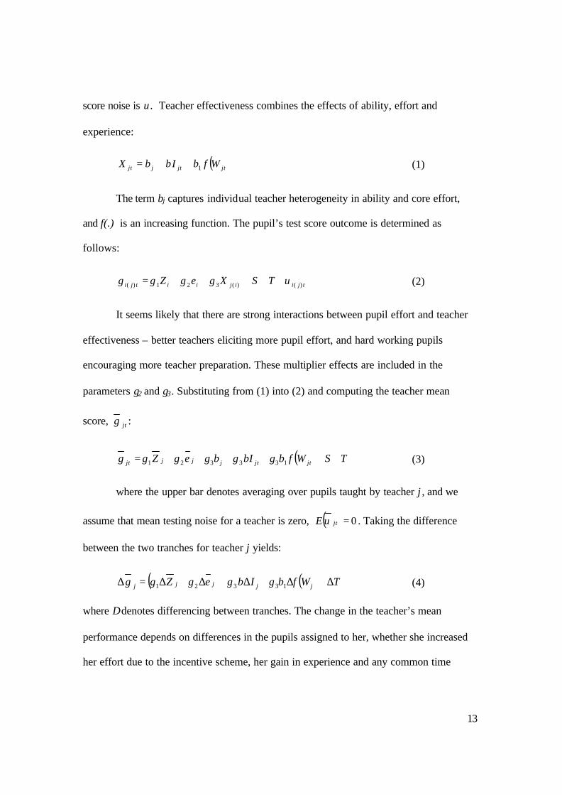
score noise is υ. Teacher effectiveness combines the effects of ability, effort and

experience:

( )jtjtjjt WfbIbX 1++= β (1)

The term bj captures individual teacher heterogeneity in ability and core effort,

and f(.) is an increasing function. The pupil’s test score outcome is determined as

follows:

tjiijiitji TSXeZg )()(321)( υγγγ +++++= (2)

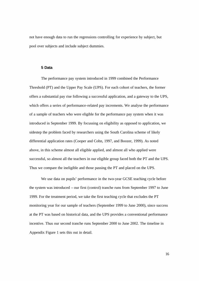
It seems likely that there are strong interactions between pupil effort and teacher

effectiveness – better teachers eliciting more pupil effort, and hard working pupils

encouraging more teacher preparation. These multiplier effects are included in the

parameters γ2 and γ3. Substituting from (1) into (2) and computing the teacher mean

score, jtg :

( ) TSWfbIbeZg jtjtjjjjt ++++++= 133321 γβγγγγ (3)

where the upper bar denotes averaging over pupils taught by teacher j , and we

assume that mean testing noise for a teacher is zero, ( ) 0=jtE υ . Taking the difference

between the two tranches for teacher j yields:

( ) ( ) TWfbIeZg jjjjj ∆+∆+∆+∆+∆=∆ 13321 γβγγγ (4)

where ∆ denotes differencing between tranches. The change in the teacher’s mean

performance depends on differences in the pupils assigned to her, whether she increased

her effort due to the incentive scheme, her gain in experience and any common time

14

shocks. Note that the fixed teacher ability term has dropped out, as has the school effect.

Finally, we compare the expected value of (4) for eligible teachers (∆I = 1) and ineligible

teachers (∆I = 0). With D denoting differencing expected values across eligibility status,

( ) ( )WfDbeDZDgD ∆++∆+∆=∆ 13321 γβγγγ (5)

This is the difference-in-difference. Assuming that the experimental design allows

us to set ( ) 021 =∆+∆ eDZDE γγ (which we discuss below), this yields

( )WfDbgD ∆+=∆ 133 γβγ . The parameter of interest is γ3β, the impact of eligibility for

the scheme on teacher effort and hence on pupil test scores. We can recover this directly

from the difference-in-difference estimates if f(.) is linear, and the second term therefore

disappears. If f(.) is concave, then gD∆ underestimates γ3β. We discuss this further

below.

The other main outcome variable we use is value-added, v. Pupil value added

depends on their effort, their teacher’s effectiveness, school and time effects and testing

noise:

tjiijitji TSXev )()(21)( ϖµµ ++++= (6)

Following the same procedure as above yields the value-added difference-in-

difference:

( ) ( )WfDbeDvD ∆++∆=∆ 1221 µβµµ (7)

We can now address the plausibility of our assumptions that

( ) 021 =∆+∆ eDZDE γγ for test scores and ( ) 01 =∆eDE µ for value-added. There is a

15

strong reason for believing that the latter holds. Pupils in England are either grouped into

classes on test outcomes, or they are not systematically grouped at all. They are not

grouped on effort, so no classes are created based on effort. Also, the timing of the

incentive scheme makes it highly unlikely that schools would be able to differentially

assign classes to eligible teachers, given that successful applications for the initial

Threshold were largely based on performance data from classes allocated prior to the

PRP scheme being introduced. So we argue that the value added results are free from any

assignment bias, and that the test score results are highly likely to be. In fact, any

difference between the results for the two outcome measures is an indication of potential

ability-based differential class assignment between eligible and ineligible teachers.

We present results for the difference-in-difference estimates in (5) and (7). As

noted, these include the effect of differential experience gain. The nature of the incentive

scheme means that ineligible teachers were necessarily less experienced than their

eligible colleagues. If f(.) is concave, then D∆f(W) will not drop out of the difference-in-

difference. We also therefore estimate regression equations for (4) and the value-added

equivalent, controlling for measures of experience.

In fact, our data allow us to differentiate outcomes by subject – English, maths

and science – and so we compute (5) and (7) separately by subject. This is useful since it

addresses spillover effects between teachers. For example, an incentivised teacher might

set a lot of homework, thus cutting students’ time for other subjects and potentially

reducing those other scores. Within subject such a spillover is not possible – if a student

has two maths teachers for example, the single maths score is attributed to both. We do

16

not have enough data to run the regressions controlling for experience by subject, but

pool over subjects and include subject dummies.

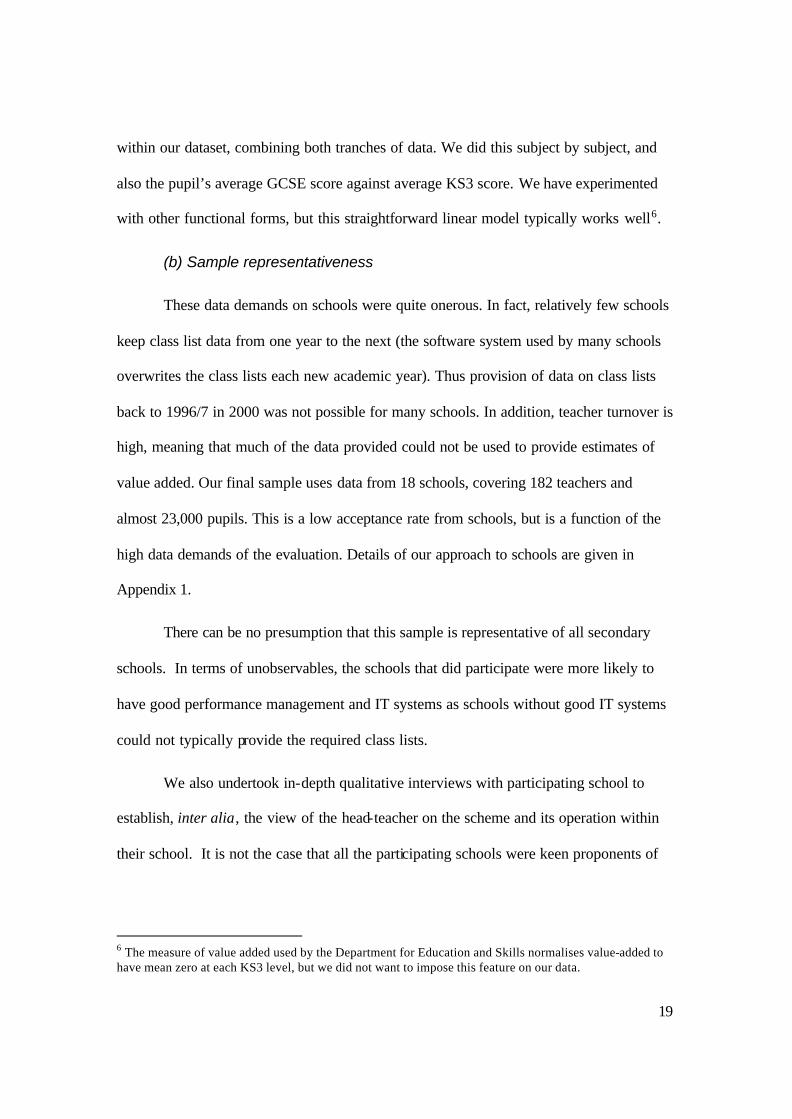
5 Data

The performance pay system introduced in 1999 combined the Performance

Threshold (PT) and the Upper Pay Scale (UPS). For each cohort of teachers, the former

offers a substantial pay rise following a successful application, and a gateway to the UPS,

which offers a series of performance-related pay increments. We analyse the performance

of a sample of teachers who were eligible for the performance pay system when it was

introduced in September 1999. By focussing on eligibility as opposed to application, we

sidestep the problem faced by researchers using the South Carolina scheme of likely

differential application rates (Cooper and Cohn, 1997, and Boozer, 1999). As noted

above, in this scheme almost all eligible applied, and almost all who applied were

successful, so almost all the teachers in our eligible group faced both the PT and the UPS.

Thus we compare the ineligible and those passing the PT and placed on the UPS.

We use data on pupils’ performance in the two-year GCSE teaching cycle before

the system was introduced – our first (control) tranche runs from September 1997 to June

1999. For the treatment period, we take the first teaching cycle that excludes the PT

monitoring year for our sample of teachers (September 1999 to June 2000), since success

at the PT was based on historical data, and the UPS provides a conventional performance

incentive. Thus our second tranche runs September 2000 to June 2002. The timeline in

Appendix Figure 1 sets this out in detail.

17

(a) Data requirements

The first key feature of the data is to control for pupil prior attainment and

measure value-added. The UK education assessment and information system provides a

number of opportunities to measure this. In this paper we examine value added between

the Key Stage 3 (KS3) exams at age 14 and the GCSE exams at age 16. Key Stage exams

are taken in English, Maths and Science; pupils also have to take GCSE exams in these

subjects (among others). The choice of the GSCE – KS3 gain is for several reasons. First,

students are mainly taught by the same teacher(s) for a particular subject throughout that

period. Second, the gap between exams is shorter than the five-year cycle between KS2

exams at 11 and GCSE exams at 16. As measuring value added requires school records

for all years in which exams are taken, a shorter focus period is easier to undertake.

Third, the GCSE exams are important for students as they are the crucial gateway

qualifications for higher education and for the employment prospects of those who leave

school at 16. Fourth, the GCSE exams are the headline component of published school

performance tables. They are thus nationally set and marked high-stakes exams for both

pupils and for schools.

The second key feature is the longitudinal element, following the same teachers

through complete KS3 – GCSE teaching cycles, one before and one during the scheme. A

detailed timeline is given in Appendix Figure 1. The scheme was introduced in the

academic year 1999/2000, with eligibility defined in September 1999, and the first forms

submitted in July 2000. The ‘before’ (tranche 1) data relate to the teaching cycle from

September 1997 through June 1999, when the GCSE exams are taken; the prior

18

attainment measure is the KS3 score from June 1997. The ‘after’ (tranche 2) data are

three years later, starting September 2000 to June 2002, with KS3 scores from June 2000.

Teachers are tagged as eligible if they were on spine point 9 in September 1999. The

evaluation design requires data that links teachers to individual pupils, before and during

the scheme. As students may be taught by a number of teachers in the two class years

between KS3 and GCSE, to create the teacher average requires that pupils be matched to

teachers for both these years, in each of the two teaching cycles. 5

The data linking pupils to teachers are class lists, which are held only by schools.

Schools therefore were approached directly initially in 2000, and invited to participate in

the study. They were told at this point that they would have to provide data for two

cohorts of pupils: those who followed the GCSE syllabus between 1997 and 1999 (the

‘before’ data) and those who followed the GCSE syllabus between 2000 and 2002 (the

‘after’ data). The data we requested from each participating school are summarised in

Table 1. The information covers 2 tranches of students: those who took their GCSEs in

1998/9 and those who took them in 2001/02. For each tranche, we requested the student’s

GCSE and KS3 scores in English, maths and science plus other pupil characteristics

including date of birth, gender and home postcode (zip code). From files on teachers we

requested information on teacher characteristics, including pay spine point, salary and

threshold eligibility, and gender. The pupil and teacher data were matched at teacher

level.

To measure pupil progress and account for prior attainment, we compute value-

added as the residual from regressing pupil GCSE score against KS3 score and gender

5 Students do not generally repeat years between KS3 and GCSE.

19

within our dataset, combining both tranches of data. We did this subject by subject, and

also the pupil’s average GCSE score against average KS3 score. We have experimented

with other functional forms, but this straightforward linear model typically works well6.

(b) Sample representativeness

These data demands on schools were quite onerous. In fact, relatively few schools

keep class list data from one year to the next (the software system used by many schools

overwrites the class lists each new academic year). Thus provision of data on class lists

back to 1996/7 in 2000 was not possible for many schools. In addition, teacher turnover is

high, meaning that much of the data provided could not be used to provide estimates of

value added. Our final sample uses data from 18 schools, covering 182 teachers and

almost 23,000 pupils. This is a low acceptance rate from schools, but is a function of the

high data demands of the evaluation. Details of our approach to schools are given in

Appendix 1.

There can be no presumption that this sample is representative of all secondary

schools. In terms of unobservables, the schools that did participate were more likely to

have good performance management and IT systems as schools without good IT systems

could not typically provide the required class lists.

We also undertook in-depth qualitative interviews with participating school to

establish, inter alia, the view of the head-teacher on the scheme and its operation within

their school. It is not the case that all the participating schools were keen proponents of

6 The measure of value added used by the Department for Education and Skills normalises value-added to have mean zero at each KS3 level, but we did not want to impose this feature on our data.

20

the reform. There was a range of views, illustrated by the following quotes (see Atkinson

and Croxson (2001a, b) for further details and analysis):

“So I'm not opposed to performance -related pay, per se … the notion of reward

for good behaviour, that's how you motivate children I think. And I don't think

adults are any different.”

“I personally am a supporter of performance-related pay. But I do have some

major misgivings about the Threshold Assessment component of it. Because my

personal view is that isn’t performance pay …the system that exists at the moment

I feel doesn’t discriminate adequately enough. It’s discriminatory measure is: is

the teacher competent or is the teacher incompetent? For example, you know, if

the outcomes of your last evaluation from OFSTED are that your teaching is

unsatisfactory then clearly you wouldn’t go for a threshold. If you’re under

current competency procedures then you wouldn’t go for the threshold. But other

than that it’s hard to see who isn’t going beyond the threshold. Because

everybody seems to be.”

“I don’t think the Performance Threshold is anything other, if I’m being crudely

honest, to sum it as being an interesting political way of giving teachers 2000

quid on the basis they’re probably Labour voters.”

Data on the performance of pupils in the sample, presented in Table 3, show a

general increase in KS3, GCSE and value added scores across all subjects from tranche 1

(1997/9) to tranche 2 (2000/02). The exception is the maths value added score, which

decreased. Table 4 uses national data from the Department for Education and Skills

(DfES) to compare the exam performance of the sample with performance at national

21

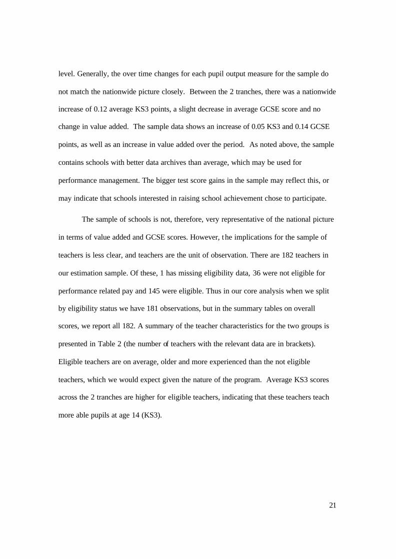
level. Generally, the over time changes for each pupil output measure for the sample do

not match the nationwide picture closely. Between the 2 tranches, there was a nationwide

increase of 0.12 average KS3 points, a slight decrease in average GCSE score and no

change in value added. The sample data shows an increase of 0.05 KS3 and 0.14 GCSE

points, as well as an increase in value added over the period. As noted above, the sample

contains schools with better data archives than average, which may be used for

performance management. The bigger test score gains in the sample may reflect this, or

may indicate that schools interested in raising school achievement chose to participate.

The sample of schools is not, therefore, very representative of the national picture

in terms of value added and GCSE scores. However, t he implications for the sample of

teachers is less clear, and teachers are the unit of observation. There are 182 teachers in

our estimation sample. Of these, 1 has missing eligibility data, 36 were not eligible for

performance related pay and 145 were eligible. Thus in our core analysis when we split

by eligibility status we have 181 observations, but in the summary tables on overall

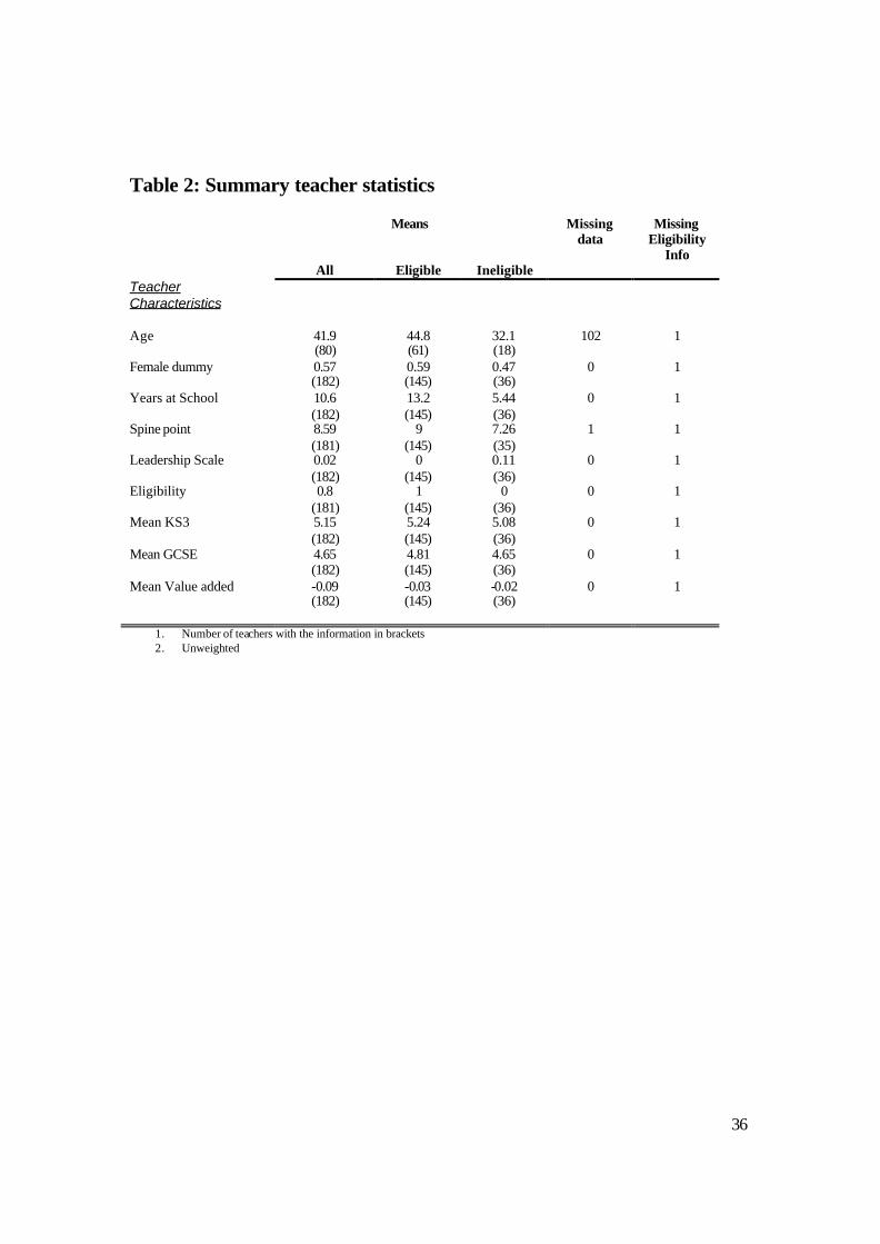
scores, we report all 182. A summary of the teacher characteristics for the two groups is

presented in Table 2 (the number of teachers with the relevant data are in brackets).

Eligible teachers are on average, older and more experienced than the not eligible

teachers, which we would expect given the nature of the program. Average KS3 scores

across the 2 tranches are higher for eligible teachers, indicating that these teachers teach

more able pupils at age 14 (KS3).

22

6 Results

We present results in three parts: first, overall teacher level outcomes; second, the

difference-in-difference analysis; third, regression analysis, and finally we provide an

interpretation. We briefly consider the potential for gaming of the scheme. Throughout,

we report weighted results, where the weights adjust for the number of pupils taught by a

teacher (unweighted results are available from the authors).

(a) Teacher level outcomes

We begin by describing the overall pattern of exam results at teacher-tranche

level, across the two two-year teaching cycles, split by the three subjects: English, maths

and science. Denote gi as pupil i’s GCSE score in a particular subject. Denote J1 as the

set of pupils taught by teacher j in tranche 1(numbering nj1), and equivalently J2 and nj2

in tranche 2. We compute teacher-tranche level summary statistics as the mean over all

pupils taught by a given teacher in a given two-year cycle7. That is, teacher-tranche mean

GCSE performance is given by 1jg and 2jg :

2

22

1

11

j

Jii

jj

Jii

j n

gg

n

gg

∑∑∈∈ == (8)

The teacher level change in GCSE performance is given by:

12 jjj ggg −=∆ (9)

the empirical counter-part to (4). Similarly, we define jjj vvv ∆and, 12 based on

pupil i’s value added, vi.

7 In all but 1 case, teachers just taught one subject, so teacher level is also implicitly subject level.

23

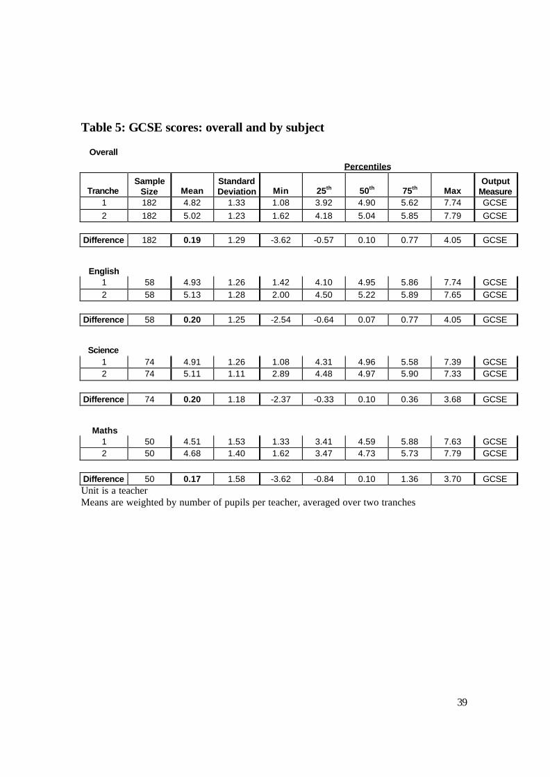
The simple GCSE results in table 5 show an overall increase in mean GCSE

scores for our teachers. The quantiles show that this was not universal and that some

teachers had considerable falls in GCSE scores between the two cycles. These patterns

are clear in the subject specific results as well.

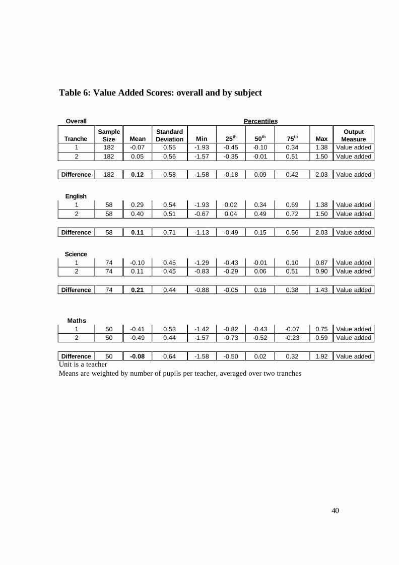
Table 6 analyses value-added. There is an overall increase in value-added

between the two dates, and in English and science, but not in maths. Again there is

considerable dispersion of the levels of teacher mean VA, and also of teacher level

changes in mean VA. For example, adding over all subjects, the biggest fall in VA is

1.58, equivalent to moving from the median VA (-0.01 in tranche 2) to the minimum (-

1.57 tranche 2). The biggest improvement is of a similar scale. As these are value -added

outcomes, they do not depend on the particular set of pupils assigned to a teacher. This

suggests considerable cycle-to-cycle variability in teacher production of value-added.

Indeed, remarkably the change in VA for a given teacher over time is as variable

(standard deviation of 0.58) as the difference between teachers in VA within a tranche

(standard deviation of 0.55).

(b) Difference in difference analysis

Figures 1 and 2 present the distribution of teacher-level GCSE and VA changes,

split by subject and by teacher eligibility status. Each panel shows a kernel estimate of

the density of the outcome variable (GCSE or VA) separately for each tranche. Some of

the plots are based on relatively small numbers of teachers.

Focussing on the GCSE plots across all subjects (the top row of Figure 1), we see

differences across eligibility status: for eligible teache rs, there is some evidence of a

rightward shift of the whole distribution in tranche 2, whereas the increase in mean GCSE

24

for ineligibles arises from a large reduction in low GCSE scores. These patterns are not

universal across subjects. The weighted VA plots across all subjects (the top row of

Figure 2) reflect a fairly similar pattern – a general rightward shift for eligibles, but a

change only in the lower half of the distribution for ineligibles.

The mean increases in scores across teaching cycles and eligibility status can be

seen in Table 7, along with some details of the distribution. Comparing the distribution

of GCSE changes across eligible and ineligible teachers, we see that the former raised

their GCSE scores by 0.21 on average and the latter by 0.13. Regressing the change in

GCSE between the two tranches against the eligibility dummy shows the difference-in-

difference of 0.08 to be insignificantly different from zero. Looking at other parts of the

distribution, we see that there are significant positive differences in the differences at the

lower quartile and the median, while the upper quartiles of the distributions show a bigger

gain for ineligibles 8. These are suggestive of a rightward shift in the lower and middle

parts of the distribution of GCSE differences for the eligible teachers. By subject, the

difference-in-difference results reveal a larger increase in mean GCSE scores for

ineligible teachers in maths and English; this is reversed in science. None of the subject

difference-in-difference estimates are significantly different from zero.

The pattern across the distribution shows considerable variation over time in

performance for a lot of teachers, illustrated in Figure 3. This plots for each teacher,

her/his mean GCSE score in tranche 1 on the horizontal axis against the equivalent in

tranche 2 on the vertical axis. Changes in performance therefore appear as deviations

from the 45o line, and eligibles and ineligibles are separately identified. Overall, there is a

8 Standard errors were derived from quantile regression.

25

greater concentration of ineligible teachers near or above the 450 line relative to those

who are eligible. We also break down the performance of teachers over the two tranches

by subject, with the largest variation appearing in maths.

However, the GCSE results depend in part on the pupils assigned to teachers in

schools. Our main focus is on VA. Figure 4 plots the comparison across the two tranches

for eligible and ineligible teachers. Again we see the considerable variation in teacher

performance between teaching cycles. The graph also shows no obviously greater

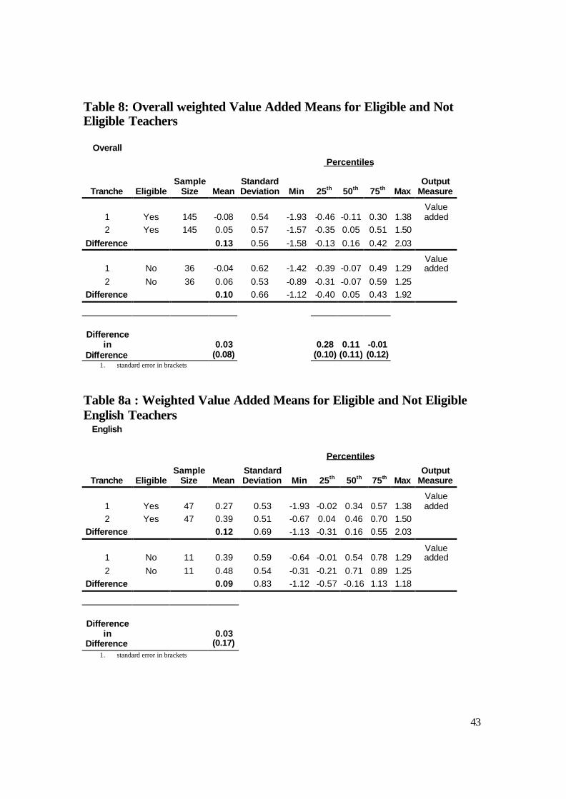
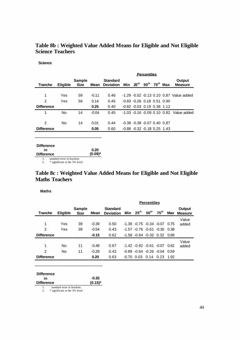
improvement for eligible teachers. Table 8 confirms this impression: VA increases

slightly more for eligible than ineligible teachers, though not significantly so. Again

considering other parts of the distribution, the lower quartile of the distribution of

differences is significantly higher for eligibles, with no significant difference at the

median or upper quartile. As with GCSE, this suggests greater impact of the scheme in

the lower half of the distribution. Looking at individual subjects, the difference-in-

difference is positive in both English and science, but much larger and negative in maths.

The overall difference-in-difference estimate is small and positive, but insignificantly

different from zero (note that the estimates for science (positive) and maths (negative) are

significantly different from zero).

The results so far suggest no clear difference between eligible and ineligible

teachers. In terms of overall value-added there is a very small and insignificantly positive

effect, arising from positive effects in science and English, and negative in maths.

However, as noted above, the difference-in-difference estimates under-estimate the

impact of the incentive scheme if the experience-effectiveness profile f(W) is concave.

We now turn to parameterising teacher experience.

26

(c) Regression Analysis

The difference-in-difference estimates control for teacher effects, (implicitly

school effects) and pupils’ prior attainment. What they do not control for, however, is the

systematic difference in experience between eligible and non-eligible teachers arising

from the nature of the performance pay scheme. If there is a positive and concave

experience-effectiveness relationship, we can only identify the impact of the incentive

scheme by controlling for differences in experience.

There is insufficient data to characterise a continuous experience-effectiveness

schedule. We do know an individual’s spine point, age and years spent at the current

school, but not their total teaching experience. The pay spine point is the best summary

of experience as teachers are rewarded for experience by movement up the pay scale.

Figures 5 and 6 plots this against teacher mean GCSE and VA outcomes. It is clear that

the mass of data at spine point 9 – the eligible set – makes it difficult to describe a clear

relationship of outcomes with experience. It also makes it difficult to separately identify

eligibility and experience.

An alternative to a smooth profile is to isolate new teachers and separate out any

substantial gains they may achieve by moving up a learning curve. We define a novice

teacher dummy, equal to 1 if the teacher is at spine point 5 or below in the first tranche.

We also define a leadership dummy, equal to 1 if the teacher is a deputy head or head

teacher.

27

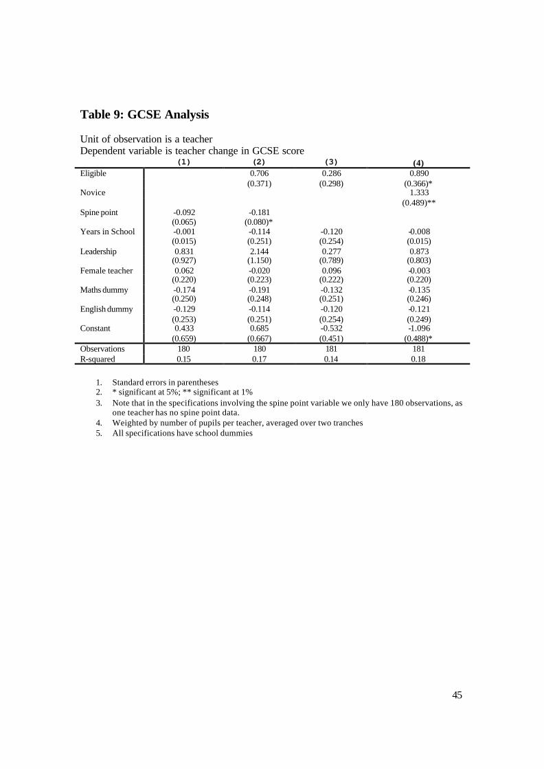
Regression results for a variety of specifications of experience are shown in Table

9 for GCSE and Table 10 for VA9. The unit of observation is a teacher, and the dependent

variable is the teacher’s change in GCSE score (respectively VA) between the two

tranches. A full set of school dummies is included, as are two subject dummies. Taking

Table 9 first, the first three columns illustrate the difficulty of trying to separately identify

eligibility and spine point as a general measure of experience. Comparing columns 1 and

2, we see that the inclusion of the eligibility dummy makes the spine point variable much

more negative – it almost doubles in size. The eligibility dummy itself is reasonably big

(and positive) but not significant. Dropping the spine point variable pushes the eligibility

dummy close to zero. In other words, high collinearity between eligibility and spine point

makes it impossible to isolate any experience effect through the spine point variable. Our

preferred specification is in column 4, in which we pick up the effect of experience

through the “novice teacher” dummy. This is large and significantly positive. Its

inclusion also yields a positive and sizeable eligibility effect, which is significant at 5%.

Of the other variables, “years in school” is always zero (conditional on the other

variables), and “leadership” role is positive but not significant. As expected, given that

we have differenced out teacher effects, the gender of the teacher appears not to matter a

great deal. We discuss the quantitative significance of the eligibility coefficient below.

The regression results for VA are shown in Table 10. These tell a very similar

story. The change in coefficients between columns 1 to 3 again reflec ts the high

correlation between eligibility and spine point. In column 4, we see that the novice

dummy is significantly positive and that eligibility is large and positive with a t-statistic

9 Note that in the specifications involving the spine point variable we only have 180 observations.

28

of 2.66. Years in school, leadership role and teacher gender again have no effect. The

consistent drop in VA in maths is clear.

In Table 11 we allow for the effect of eligibility to vary between subjects,

reporting specifications equivalent to column 4 in Tables 9 and 10. This is suggested by

the difference-in-difference findings above. We see that for GCSE, the eligibility dummy

is positive and well-defined. The interaction with the maths subject dummy is negative

and of similar size, but not significant. In the case of VA, the eligibility coefficient is

positive and now well-defined10. Again, the maths interaction is equal and opposite in

sign, and this time is significant. The sample of maths teachers is not different in terms of

observables to the other subject teachers – very similar age and experience patterns and a

gender ratio between English and science.

We are interested to see whether the incentive scheme had a constant impact

across the ability range, or had differential impacts. To get at this, we compute for each

teacher the difference between the k th percentile of the outcome distribution for tranche 2

and subtract from that the k th percentile of the outcome distribution for tranche 1. So this

is not the difference in mean performance for each teacher, but the difference in

performance across the distribution. We do this for k = 10, 25, 50, 75 and 90. We regress

these outcome differences against eligibility and the other variables as in the previous

Table. The results in Table 12 simply report the eligibility coefficient. There is no clear

overall pattern in this for GCSE, but for VA the coefficient is considerably higher (by

about a third) at the bottom two points than higher up. This suggests that the incentive

10 If we allow the errors to be clustered at school level, the results carry through – the standard error for eligibility status in the GCSE regression rises from 0.437 to 0.440 with clustering against a coefficient of 1.339, and in the VA regression it rises from 0.180 to 0.205 with a coefficient of 0.653.

29

scheme had greater impact on raising scores among low achievers, possibly because

teachers concentrated their efforts where they thought easier gains were to be made.

While this may be related to ceiling effects (see next section), the fact that it appears in

the bottom quarter suggests there is a real effect too.

(d) Robustness checks

We use the novice teacher dummy to capture the experience profile and identify

the effect of the scheme. To check our degree of reliance on the novice dummy, we

instead drop all novices from the estimation and re-estimate. In this case, identification

comes from a comparison of eligible and non-eligible teachers with a similar level of

experience. The first two columns of Table 13 show that this makes a marginal difference

to our results: the estimated impacts of eligibility are in fact marginally higher at 1.389

for GCSE and is 0.786 for VA, compared to 1.339 and 0.653 in Table 1111. This is

reassuring that the use of the novice teacher dummy is not too restrictive.

A second problem may be the presence of ceiling effects in test scores. Both in

GCSE and more particularly VA, there is an upper limit to the grade a student can be

awarded, and therefore to the progress that they can be measured to make in our measure

of VA. This problem will differ between classes depending on ability distribution, and so

might affect the score gain that we attribute to the scheme. One simple way to deal with

this is to consider the bottom 75% of the pupil distribution only (the bottom 75% of the

initial KS3 distribution), and we report the results in columns 3 and 4 of Table 13. They

show similar coefficients on eligibility status, slightly lower than in Table 11.

11 Note that the interaction with English is now significantly negative.

30

(e) Gaming

The obvious way that a school could try to help its teachers succeed would be to

assign them classes in which they could more easily demonstrate above-average pupil

progress. In fact, the timing of the start of the school year and the deadline for the

submission of applications mean that this is very unlikely. Applications for the initial

Threshold, submitted in July 2000, were largely based on performance data from classes

allocated prior to the announcement of the PRP scheme, so differential allocation of

classes between eligible and non-eligible teachers in our ‘before’ data does is not a

credible gaming strategy. Also, our data suggest little change in class assignment between

the two tranches – the mean KS3 average of pupils taught by eligible teachers rose from

5.167 in tranche 1 to 5.290 in tranche (a difference of 0.123), and from 4.989 to 5.191 for

ineligibles (0.202). These are both small changes, and the difference between them is

only around 1.5% of the tranche 1 scores. There is no support here for systematic changes

in class assignment. There is some evidence that Headteachers did help with filling in the

paperwork (Wragg et al 2001), but this will have no effect on pupil test scores in national

exams.

(f) Evaluation

We evaluate the size of the coefficient on eligibility status in two ways. Both

GCSE and VA changes are in the same metric of GCSE points (the latter is just a residual

of the former), and one point is the difference between a grade (an ‘A’ and a ‘B’ for

example). As we have seen above (Tables 5 and 6), one standard deviation in the teacher -

mean change in GCSE is 1.29 and for VA is 0.58. We can compare these to the

coefficients on eligibility of 0.890 for GCSE change (Table 9, column 4) and 0.422 for

31

VA change (Table 10, column 4); as percentages of a standard deviation these are 69%

and 73% respectively. In terms of straightforward grades, the estimates suggest that the

scheme added on average almost ha lf a grade of VA per child for eligible teachers. These

are substantial effects in high-stakes exams: GCSEs are the gateway exams into higher

education. It makes no sense to incorporate these results into a cost-benefit analysis of the

scheme, since we only capture the incentivisation aspect here and not the recruitment and

retention aspect.

An alternative way of thinking about the impact of the scheme is to note that the

eligibility dummy is about 67% of the size of the novice teacher dummy for GCSE

change, and 78% for VA change. Thus the incentive scheme can be thought of as eliciting

extra effort equivalent to about three-quarters of the effect of young teachers moving up

the learning curve.

It would be of interest to distinguish between those among the eligible who passed

the Threshold, and so reached the UPS, and those who did not. In practice, this is not

possible. As we noted above, nationally 97% of the eligible passed the Threshold, so a

distinction between the groups is largely impossible. In our dataset, information on

whether a teacher passed is missing for some teachers, so we are unable to confirm this

figure for our sample. It seems very likely that almost all of these in fact passed the

Threshold, and hence we cannot distinguish between those passing and those not.

32

7 Conclusion

This paper evaluates the impact of a performance-related pay system for teachers

in England. Using teacher level data, matched with pupil test scores and value-added, we

test whether the introduction of a payment based on pupil attainment increased teacher

effort. Our evaluation design controls for pupil effects, school effects and teacher effects,

and adopts a difference-in-difference methodology.

We find that the scheme did improve test score gains, on average by about half a

grade per pupil. We also found heterogeneity across subject teachers, with maths teachers

showing no improvement. A caveat is the necessity, given our data, to define the

experience-effectiveness profile in quite a parametric way. Nevertheless, our results add

to the very small literature on individual teacher-based performance pays schemes,

evaluated in the context of a robust research design. The results show that teachers do

respond to direct financial incentives. In an incentive scheme strongly based on pupil

progress, test scores improved. Whether this represented extra effort or effort diverted

from other professional activities is not something we can determine in our dataset. But

our results suggest that teacher-based performance pay is a policy tool that education

authorities should consider as part of their drive to raise educational performance.

33

References Boozer, M. A. (1999). The Design and Evaluation of Incentive Schemes for Schools:

Evidence from South Carolina’s Teacher Incentive Pay Project. Mimeo, Hoover Institute

Burgess, S. and M. Ratto (2003), The Role of Incentives in the Public Sector: Issues and Evidence, Oxford Review of Economic Policy, 19(2): 285-300

Cooper, S. T. and E. Cohn (1997). "Estimation of a Frontier Production Function for the South Carolina Educational Process." Economics of Education Review 16(3): 313-327.

Courty, Pascal & Marschke, Gerald, (2001) Performance Incentives with Award Constraints, CEPR Discussion Papers 2720

Croxson, B and A Atkinson (2001a) The implementation of the Performance Threshold in UK secondary schools, CMPO Working Paper 01/044, CMPO, University of Bristol.

Croxson, B and A Atkinson (2001b) Incentives in secondary schools: the impact of the Performance Threshold , CMPO Working Paper 01/045, CMPO, University of Bristol.

Dee, T. S. and B. J. Keys (2004). Does Merit Pay Reward Good Teachers? Evidence From a Randomized Experiment, Journal of Policy Analysis and Management 23(3): 471-488.

DfEE (2000) Threshold Assessment Application Pack, DfEE, London.

Dixit, A. (2002). Incentives and Organizations in the Public Sector: An Interpretative Review, Journal of Human Resources, 37(4): 696-727.

Eberts, R., K. Hollenbeck, et al. (2002). Teacher Performance Incentives and Student Outcomes, Journal of Human Resources 37(4): 913-927

Figlio, D. N. and L. W. Kenny (2003). Do Individual Teacher Incentives Boost Student Performance?, University of Florida.

Glennerster, H (1991) Quasi-markets for education? Economic Journal, 101(408): 1268-1276

Glewwe, P., N. Ilias, et al. (2003). Teacher Incentives, NBER Working Paper, 9671.

Hanushek, E. A. (2003) ‘The Failure of Input-based Schooling Policies’. Economic Journal vol. 113, pp. F64-F98

Hood, C, C Scott, O James, G Jones and T Travers (1999) Regulation inside government: waste-watchers, quality policy and sleaze busters, Oxford University Press, Oxford.

Khan, C., Silva, E. and Ziliak, J. (2001) Performance-Based Wages in Tax Collection: The Brazilian Tax Collection Reform and Its Effects, Economic Journal 111(468), 188-205.

34

Ladd, H. (1999). The Dallas school accountability and incentive program: an evaluation of its impacts on student outcomes, Economics of Education Review 18: 1-16.

Lavy, V. (2002a). Evaluating the Effect of Teacher Group Performance Incentive s on Students Achievements, Journal of Political Economy 110 (6): 1286-1317

Lavy, V. (2003). Paying for Performance: The Effect of Individual Financial Incentives on Teachers' Productivity and Students' Scholastic Outcomes , CEPR Discussion Papers, 3862

Lavy, V. (2004). Performance Pay and Teachers' Effort, Productivity and Grading Ethics, NBER Working Paper, 10622.

Lazear, E. (2003) Teacher Incentives. Swedish Economic Policy Review vol. 10 no. 2 pp. 179 – 214.

Marsden, D and S French (1998) What a performance: performance related pay in the public services, Centre for Economic Performance, LSE, London.

Marsden, D. (2000) Teachers Before the 'Threshold'. CEP Discussion paper 454, LSE.

Murphy, K (1999) Executive Compensation in: O. Ashenfelter and D.Card, eds., Handbook of Labor Economics, North Holland.

Prendergast, C. The Provision of Incentives in Firms. Journal of Economic Literature, 1999, 37(1): 7-63.

Tomlinson, H (1992) Performance related pay in education , Routledge, London.

Tomlinson, H (2000) Proposals for performance related pay for teachers in English schools, School Leadership and Management, 20: 281-298

Wilson, D (2004) Which ranking? The impact of a ‘value added’ measure of secondary school performance, Public Money and Management, 24(1): 37-45.

Wragg, E, G Haynes, C Wragg and R Chamberlin (2001) Performance related pay: the views and experiences of 1000 primary and secondary headteachers, Teachers’ Incentives Pay Project Occasional Paper 1, School of Education, University of Exeter.

35

Table 1: Data Requested Information Level Class lists for year 10 in 1997/8 and year 11 in 1998/9, with pupil identifiers and teacher identifiers

pupil

Class lists for year 10 in 2000/1 and year 11 in 2001/2, with pupil identifiers and teacher identifiers

pupil

Pupil test/exam scores for Key Stage 3 in 1996/7 and GCSE 1998/9, for all English, maths and science subjects, with pupil identifiers

pupil

Pupil test/exam scores for Key Stage 3 in 1999/00 and GCSE 2001/02, for all English, maths and science subjects, with pupil identifiers

pupil

Supplementary information for each pupil: date of birth, gender, postcode. With pupil identifier

pupil

Teachers characteristics at 1 September 1999: age, gender, salary, experience, spine point, whether applied for PT. With teacher identifier

teacher

Information about school policy: exam boards used, streaming/setting policy, pre-existing performance management system

school

36

Table 2: Summary teacher statistics Means Missing

data Missing

Eligibility Info

All Eligible Ineligible Teacher Characteristics

Age

41.9 (80)

44.8 (61)

32.1 (18)

102 1

Female dummy

0.57 (182)

0.59 (145)

0.47 (36)

0 1

Years at School

10.6 (182)

13.2 (145)

5.44 (36)

0 1

Spine point

8.59 (181)

9 (145)

7.26 (35)

1 1

Leadership Scale 0.02 (182)

0 (145)

0.11 (36)

0 1

Eligibility 0.8 (181)

1 (145)

0 (36)

0 1

Mean KS3

5.15 (182)

5.24 (145)

5.08 (36)

0 1

Mean GCSE

4.65 (182)

4.81 (145)

4.65 (36)

0 1

Mean Value added

-0.09 (182)

-0.03 (145)

-0.02 (36)

0 1

1. Number of teachers with the information in brackets 2. Unweighted

37

Table 3: Summary pupil statistics Tranche 1 Tranche 2 Pupil Characteristics

Gender 0.53 (10777)

0.50 (12170)

KS3

5.29 (10611)

5.34 (11902)

English

5.12 (2706)

5.13 (2865)

Science

5.34 (5515)

5.53 (6418)

Maths

5.39 (2386)

5.53 (2619)

GCSE 4.88 (10717)

5.02 (11559)

English 5.04 (2805)

5.16 (2879)

Science 4.92 (5493)

5.11 (6044)

Maths 4.62 (2415)

4.65 (2636)

Value added

-0.04 (9830)

0.03 (11140)

English

0.33 (2593)

0.39 (2786)

Science

-0.07 (4970)

0.09 (5809)

Maths

-0.38 (2263)

-0.49 (2545)

1. Number of pupils with the information in brackets 2. Unweighted 3. VA is the residual from the pupil level regression of GCSE against KS3 and a female dummy

38

Table 4: Comparative Summary statistics for National and Estimation data sets

National

Estimation

Tranche 1 Tranche 2 Difference Tranche 1 Tranche 2 Difference KS3

English

4.66 (0.0022)

4.82 (0.0021)

0.16 (0.0031)

5.12 5.13 0.01

Science

4.93 (0.0017)

4.88 (0.0018)

-0.05 (0.0024)

5.39 5.53 0.14

Maths

5.02 (0.0019)

5.24 (0.0019)

0.22 (0.0027)

5.33 5.36 0.03

Overall 4.87 (0.0013)

4.99 (0.0011)

0.12 (0.0016)

5.29 5.34 0.05

GCSE

English

4.82 (0.0024)

4.81 (0.0022)

-0.01 (0.0003)

5.04 5.16 0.12

Science

4.32 (0.0026)

4.21 (0.0024)

-0.11 (0.0035)

4.92 5.11 0.19

Maths

4.13 (0.0027)

4.21 (0.0025)

0.08 (0.0037)

4.62 4.65 0.03

Overall 4.42 (0.0015)

4.41 (0.0014)

-0.01 (0.0020)

4.88 5.02 0.14

Value added

English

0.553 (0.0017)

0.504 (0.0016)

-0.049 (0.002)

0.33 0.39 0.06

Science

-0.132 (0.0017)

-0.074 (0.0015)

0.058 (0.002)

-0.07 0.09 0.16

Maths

-0.425 (0.0016)

-0.427 (0.0014)

-0.002 (0.002)

-0.38 -0.49 -0.11

Overall -0.002 (0.0010)

0.002 (0.0009)

0.004 (0.0014)

-0.04 0.03 0.07

Source: Department for Education and Skills Authors’ calculations using Pupil-level Annual Schools Census

Standard deviations for national data in parentheses

39

Table 5: GCSE scores: overall and by subject

Overall

Percentiles

Tranche Sample

Size Mean Standard Deviation Min 25th 50th 75th Max

Output Measure

1 182 4.82 1.33 1.08 3.92 4.90 5.62 7.74 GCSE 2 182 5.02 1.23 1.62 4.18 5.04 5.85 7.79 GCSE

Difference 182 0.19 1.29 -3.62 -0.57 0.10 0.77 4.05 GCSE

English 1 58 4.93 1.26 1.42 4.10 4.95 5.86 7.74 GCSE 2 58 5.13 1.28 2.00 4.50 5.22 5.89 7.65 GCSE

Difference 58 0.20 1.25 -2.54 -0.64 0.07 0.77 4.05 GCSE

Science 1 74 4.91 1.26 1.08 4.31 4.96 5.58 7.39 GCSE 2 74 5.11 1.11 2.89 4.48 4.97 5.90 7.33 GCSE

Difference 74 0.20 1.18 -2.37 -0.33 0.10 0.36 3.68 GCSE

Maths 1 50 4.51 1.53 1.33 3.41 4.59 5.88 7.63 GCSE 2 50 4.68 1.40 1.62 3.47 4.73 5.73 7.79 GCSE

Difference 50 0.17 1.58 -3.62 -0.84 0.10 1.36 3.70 GCSE Unit is a teacher Means are weighted by number of pupils per teacher, averaged over two tranches

40

Table 6: Value Added Scores: overall and by subject

Overall Percentiles

Tranche Sample


Output Measure

1 182 -0.07 0.55 -1.93 -0.45 -0.10 0.34 1.38 Value added 2 182 0.05 0.56 -1.57 -0.35 -0.01 0.51 1.50 Value added

Difference 182 0.12 0.58 -1.58 -0.18 0.09 0.42 2.03 Value added

English 1 58 0.29 0.54 -1.93 0.02 0.34 0.69 1.38 Value added 2 58 0.40 0.51 -0.67 0.04 0.49 0.72 1.50 Value added


Science 1 74 -0.10 0.45 -1.29 -0.43 -0.01 0.10 0.87 Value added 2 74 0.11 0.45 -0.83 -0.29 0.06 0.51 0.90 Value added


Maths 1 50 -0.41 0.53 -1.42 -0.82 -0.43 -0.07 0.75 Value added 2 50 -0.49 0.44 -1.57 -0.73 -0.52 -0.23 0.59 Value added

Difference 50 -0.08 0.64 -1.58 -0.50 0.02 0.32 1.92 Value added Unit is a teacher Means are weighted by number of pupils per teacher, averaged over two tranches

41

Table 7: Overall Weighted GCSE Means for Eligible and Not Eligible Teachers Overall

Percentiles

Tranche Eligible Sample


Output Measure

1 Yes 145 4.84 1.30 1.33 3.99 4.90 5.58 7.74 GCSE 2 Yes 145 5.05 1.28 1.62 4.12 5.12 5.90 7.79

Difference 0.21 1.24 -3.62 -0.29 0.16 0.75 4.05 1 No 36 4.78 1.50 1.08 3.81 5.26 5.71 6.90 GCSE 2 No 36 4.91 1.05 2.33 4.30 4.71 5.73 7.08

Difference 0.13 1.53 -1.91 -0.88 -0.64 1.23 3.70

Difference in

Difference 0.08

(0.17) 0.59

(0.10) 0.81

(0.11) -0.47 (0.38)

1. standard error in brackets Table 7a: Weighted GCSE Means for Eligible and Not Eligible English Teachers

English

Percentiles



Output Measure

1 Yes 47 4.91 1.28 1.42 4.10 4.95 5.54 7.74 GCSE 2 Yes 47 5.10 1.34 2.00 4.12 5.22 5.93 7.65

Difference 0.19 1.22 -2.54 -0.34 0.12 0.77 4.05

1 No 11 5.01 1.25 3.00 4.58 5.52 6.04 6.39 GCSE 2 No 11 5.25 1.00 3.21 4.71 5.38 5.88 7.08

Difference 0.24 1.39 -1.21 -0.64 0.06 1.30 2.80

Difference in

Difference -0.05 (0.30)

1. standard error in brackets

42

Table 7b: Weighted GCSE Means for Eligible and Not Eligible Science Teachers

Science

Percentiles



Output Measure

1 Yes 59 4.91 1.22 1.92 4.31 4.96 5.43 7.39 GCSE 2 Yes 59 5.19 1.11 2.89 4.64 5.15 5.90 7.33


Difference -0.14 1.54 -1.91 -0.88 -0.78 0.05 3.68

Difference in

Difference 0.42

(0.25) 1. standard error in brackets Table 7c: Weighted GCSE Means for Eligible and Not Eligible Maths Teachers

Maths

Percentiles



Output Measure

1 Yes 39 4.57 1.49 1.33 3.45 4.59 5.88 7.63 GCSE 2 Yes 39 4.63 1.50 1.62 3.40 4.73 5.96 7.79


Difference 0.58 1.65 -1.72 -0.65 0.00 1.85 3.70

Difference in

Difference -0.52 (0.39)


43

Table 8: Overall weighted Value Added Means for Eligible and Not Eligible Teachers

Overall

Percentiles



Output Measure

1 Yes 145 -0.08 0.54 -1.93 -0.46 -0.11 0.30 1.38 Value added

2 Yes 145 0.05 0.57 -1.57 -0.35 0.05 0.51 1.50 Difference 0.13 0.56 -1.58 -0.13 0.16 0.42 2.03

1 No 36 -0.04 0.62 -1.42 -0.39 -0.07 0.49 1.29 Value added

2 No 36 0.06 0.53 -0.89 -0.31 -0.07 0.59 1.25 Difference 0.10 0.66 -1.12 -0.40 0.05 0.43 1.92

Difference in

Difference 0.03

(0.08) 0.28

(0.10) 0.11

(0.11) -0.01 (0.12)


Table 8a : Weighted Value Added Means for Eligible and Not Eligible English Teachers

English

Percentiles



Output Measure

1 Yes 47 0.27 0.53 -1.93 -0.02 0.34 0.57 1.38 Value added

2 Yes 47 0.39 0.51 -0.67 0.04 0.46 0.70 1.50 Difference 0.12 0.69 -1.13 -0.31 0.16 0.55 2.03

1 No 11 0.39 0.59 -0.64 -0.01 0.54 0.78 1.29 Value added

2 No 11 0.48 0.54 -0.31 -0.21 0.71 0.89 1.25 Difference 0.09 0.83 -1.12 -0.57 -0.16 1.13 1.18

Difference in

Difference 0.03

(0.17) 1. standard error in brackets

44

Table 8b : Weighted Value Added Means for Eligible and Not Eligible Science Teachers

Science

Percentiles



Output Measure

1 Yes 59 -0.11 0.46 -1.29 -0.52 -0.13 0.10 0.87 Value added 2 Yes 59 0.14 0.45 -0.83 -0.26 0.18 0.51 0.90

Difference 0.25 0.40 -0.82 -0.03 0.19 0.38 1.12

1 No 14 -0.04 0.45 -1.03 -0.16 -0.09 0.10 0.82 Value added

2 No 14 0.01 0.44 -0.38 -0.38 -0.07 0.40 0.87 Difference 0.05 0.60 -0.88 -0.32 -0.18 0.25 1.43

Difference in

Difference 0.20

(0.09)* 1. standard error in brackets 2. * significant at the 5% level.

Table 8c : Weighted Value Added Means for Eligible and Not Eligible Maths Teachers

Maths

Percentiles



Output Measure

1 Yes 39 -0.39 0.50 -1.39 -0.75 -0.34 -0.07 0.75 Value added

2 Yes 39 -0.54 0.43 -1.57 -0.76 -0.61 -0.30 0.38 Difference -0.15 0.62 -1.58 -0.64 -0.02 0.32 0.89

1 No 11 -0.48 0.67 -1.42 -0.92 -0.61 -0.07 0.62 Value added

2 No 11 -0.28 0.43 -0.89 -0.64 -0.26 -0.04 0.59 Difference 0.20 0.63 -0.70 0.03 0.14 0.23 1.92

Difference in

Difference -0.35

(0.15)* 1. standard error in brackets

2. * significant at the 5% level.

45

Table 9: GCSE Analysis Unit of observation is a teacher Dependent variable is teacher change in GCSE score (1) (2) (3) (4) Eligible 0.706 0.286 0.890 (0.371) (0.298) (0.366)* Novice 1.333 (0.489)** Spine point -0.092 -0.181 (0.065) (0.080)* Years in School -0.001 -0.114 -0.120 -0.008 (0.015) (0.251) (0.254) (0.015) Leadership 0.831 2.144 0.277 0.873 (0.927) (1.150) (0.789) (0.803) Female teacher 0.062 -0.020 0.096 -0.003 (0.220) (0.223) (0.222) (0.220) Maths dummy -0.174 -0.191 -0.132 -0.135 (0.250) (0.248) (0.251) (0.246) English dummy -0.129 -0.114 -0.120 -0.121 (0.253) (0.251) (0.254) (0.249) Constant 0.433 0.685 -0.532 -1.096 (0.659) (0.667) (0.451) (0.488)* Observations 180 180 181 181 R-squared 0.15 0.17 0.14 0.18

1. Standard errors in parentheses 2. * significant at 5%; ** significant at 1% 3. Note that in the specifications involving the spine point variable we only have 180 observations, as

one teacher has no spine point data. 4. Weighted by number of pupils per teacher, averaged over two tranches 5. All specifications have school dummies

46

Table 10: Value Added Analysis Unit of observation is a teacher Dependent variable is teacher change in VA score (1) (2) (3) (4) Eligible 0.193 0.063 0.422 (0.173) (0.128) (0.152)** Novice 0.539 (0.203)** Spine point -0.022 -0.057 (0.027) (0.033) Years in School -0.003 -0.005 -0.006 -0.005 (0.006) (0.006) (0.006) (0.006) Leadership 0.045 0.556 -0.005 0.236 (0.381) (0.473) (0.327) (0.333) Female teacher -0.014 -0.046 -0.001 -0.040 (0.091) (0.092) (0.092) (0.091) English dummy -0.145 -0.139 -0.134 -0.134 (0.104) (0.103) (0.105) (0.103) Maths dummy -0.337 -0.344 -0.315 -0.317 (0.103)** (0.102)** (0.104)** (0.102)** Constant 0.308 0.407 -0.021 -0.249 (0.271) (0.275) (0.187) (0.202) Observations 180 180 181 181 R-squared 0.27 0.29 0.26 0.29



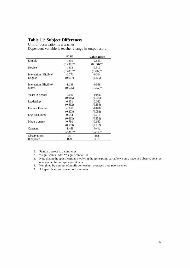
47

Table 11: Subject Differences Unit of observation is a teacher Dependent variable is teacher change in output score GCSE Value added Eligible 1.339 0.653 (0.437)** (0.180)** Novice 1.313 0.511 (0.480)** (0.202)* Interaction: Eligible* -0.771 -0.394 English

(0.667) (0.275)

Interaction: Eligible* -1.138 -0.588 Maths

(0.625) (0.257)*

Years in School -0.010 -0.006 (0.015) (0.006) Leadership 0.531 0.062 (0.862) (0.355) Female Teacher -0.059 -0.070 (0.223) (0.092) English dummy 0.554 0.211 (0.612) (0.252) Maths d ummy 0.791 0.162 (0.563) (0.232) Constant -1.468 -0.441 (0.524)** (0.216)* Observations 181 181 R-squared 0.20 0.31



48

Table 12: Distributional Impacts Unit of observation is a teacher Dependent variable is: (kth percentile of outcome distribution for tranche 2 for teacher j) – (kth percentile of outcome distribution for tranche 1 for teacher j) Coefficient on Eligibility: GCSE Value added

Percentile 10th 1.145 0.849 (0.516)* (0.246)** 25th 1.394 0.856 (0.465)** (0.220)** 50th 1.394 0.689 (0.465)** (0.224)** 75th 1.753 0.562 (0.499)** (0.216)* 90th 1.308 0.637 (0.522)* (0.294)*

1. Standard errors in parentheses 2. * significant at 5%; ** significant at 1% 3. Weighted by number of pupils per teacher, averaged over 2 tranches 4. All specifications have school dummies 5. Each cell reports coefficient from a different regression 6. Other variables included as in Table 11 7. All regressions have 181 observations

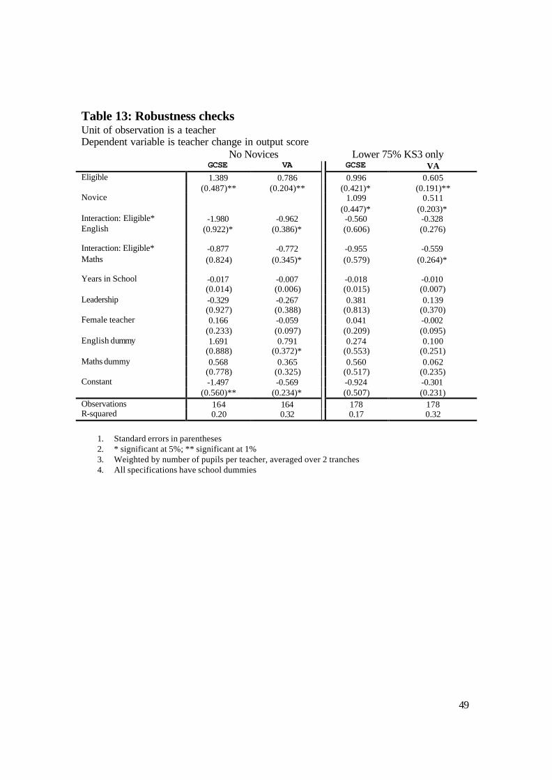
49

Table 13: Robustness checks Unit of observation is a teacher Dependent variable is teacher change in output score No Novices Lower 75% KS3 only GCSE VA GCSE VA Eligible 1.389 0.786 0.996 0.605 (0.487)** (0.204)** (0.421)* (0.191)** Novice 1.099 0.511 (0.447)* (0.203)* Interaction: Eligible* -1.980 -0.962 -0.560 -0.328 English

(0.922)* (0.386)* (0.606) (0.276)

Interaction: Eligible* -0.877 -0.772 -0.955 -0.559 Maths

(0.824) (0.345)* (0.579) (0.264)*

Years in School -0.017 -0.007 -0.018 -0.010 (0.014) (0.006) (0.015) (0.007) Leadership -0.329 -0.267 0.381 0.139 (0.927) (0.388) (0.813) (0.370) Female teacher 0.166 -0.059 0.041 -0.002 (0.233) (0.097) (0.209) (0.095) English dummy 1.691 0.791 0.274 0.100 (0.888) (0.372)* (0.553) (0.251) Maths dummy 0.568 0.365 0.560 0.062 (0.778) (0.325) (0.517) (0.235) Constant -1.497 -0.569 -0.924 -0.301 (0.560)** (0.234)* (0.507) (0.231) Observations 164 164 178 178 R-squared 0.20 0.32 0.17 0.32

1. Standard errors in parentheses 2. * significant at 5%; ** significant at 1% 3. Weighted by number of pupils per teacher, averaged over 2 tranches 4. All specifications have school dummies

50

Figure 1: Distribution of teacher outcomes: GCSE Kernel de nsity estimates over teacher mean scores Overall

0

.1

.2

.3

.4

0 2 4 6 8 GCSE

Tranche 1 Tranche 2

Eligible Kdensity plot for Weighted GCSE in both tranches

Den

sity

0

.1

.2

.3

.4

0 2 4 6 8 GCSE

Tranche 1 Tranche 2

Not Eligible Kdensity plot for Weighted GCSE in both tranches

Den

sity

English

0

.1

.2

.3

.4

0 2 4 6 8 GCSE

Tranche 1 Tranche 2

Eligible Kdensity plot for English Weighted GCSE in both tranches

Den

sity

0

.1

.2

.3

.4

0 2 4 6 8 GCSE

Tranche 1 Tranche 2

Not Eligible Kdensity plot for English Weighted GCSE in both tranches

Den

sity

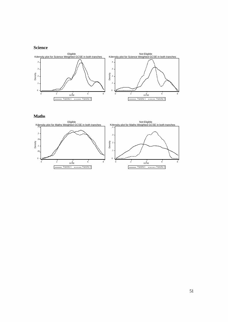
51

Science

0

.1

.2

.3

.4

0 2 4 6 8 GCSE

Tranche 1 Tranche 2

Eligible Kdensity plot for Science Weighted GCSE in both tranches

Den

sity

0

.1

.2

.3

.4

0 2 4 6 8 GCSE

Tranche 1 Tranche 2

Not Eligible Kdensity plot for Science Weighted GCSE in both tranches

Den

sity

Maths

0

.05

.1

.15

.2

.25

0 2 4 6 8 GCSE

Tranche 1 Tranche 2

Eligible Kdensity plot for Maths Weighted GCSE in both tranches

Den

sity

0

.1

.2

.3

.4

0 2 4 6 8 GCSE

Tranche 1 Tranche 2

Not Eligible Kdensity plot for Maths Weighted GCSE in both tranches

Den

sity

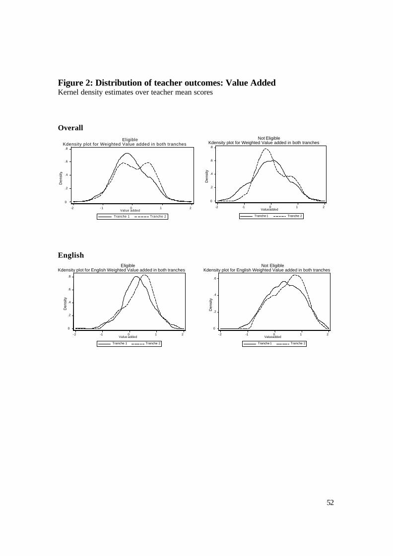
52

Figure 2: Distribution of teacher outcomes: Value Added Kernel density estimates over teacher mean scores Overall

0

.2

.4

.6

.8

Den

sity

-2 -1 0 1 2 Value added

Tranche 1 Tranche 2

Eligible Kdensity plot for Weighted Value added in both tranches

0

.2

.4

.6

.8

Den

sity

-2 -1 0 1 2 Valueadded

Tranche 1 Tranche 2

Not Eligible Kdensity plot for Weighted Value added in both tranches

English

0

.2

.4

.6

.8

Den

sity


Tranche 1 Tranche 2

Eligible Kdensity plot for English Weighted Value added in both tranches

0

.2

.4

.6


Tranche 1 Tranche 2

Not Eligible Kdensity plot for English Weighted Value added in both tranches

Den

sity

53

Science

0

.2

.4

.6

.8

Den

sity


Tranche 1 Tranche 2

Eligible Kdensity plot for Science Weighted Value added in both tranches

0

.5

1

1.5 2


Tranche 1 Tranche 2

Not Eligible Kdensity plot for Science Weighted Value added in both tranches

Den

sity

Maths

0 .2 .4 .6 .8 1


Tranche 1 Tranche 2

Eligible Kdensity plot for Maths Weighted Value added in both tranches

Den

sity

0

.2

.4

.6

.8


Tranche 1 Tranche 2

Not Eligible Kdensity plot for Maths Weighted Value added in both tranches

Den

sity

54

Figure 3: Comparing tranche 1 and tranche 2 Unit is a teacher. The line is 45°

0

2

4

6

8 GC

SE

score in tranche 2

0 2 4 6 8 GCSE score in tranche 1

Eligible Not eligible

Mean GCSE score in tranche2 against Mean GCSE in tranche1

0

2

4

6

8

GC

SE

score in tranche 2



Mean GCSE score in tranche 2 against Mean GCSE in tranche1 English

0

2

4

6

8

GC

SE

score in tranche 2



Mean GCSE score in tranche 2 against Mean GCSE in tranche1 for Science

0

2

4

6

8

GC

SE

score in tranche 2



Mean GCSE score in tranche 2 against Mean GCSE in tranche1 for Maths

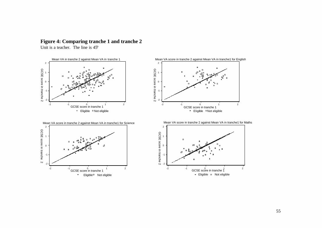
55

Figure 4: Comparing tranche 1 and tranche 2 Unit is a teacher. The line is 45°

-2

-1

0

1

2

GC

SE

score in tranche 2

-2 -1 0 1 2 GCSE score in tranche 1


Mean VA in tranche 2 against Mean VA in tranche 1

-2

-1

0

1

2

GC

SE

score in tranche 2



Mean VA score in tranche 2 against Mean VA in tranche1 for English

-2

-1

0

1

2 GC

SE

score in tranche 2



Mean VA score in tranche 2 against Mean VA in tranche1 for Science

-2

-1

0

1

2

GC

SE

score in tranche 2



Mean VA score in tranche 2 against Mean VA in tranche1 for Maths

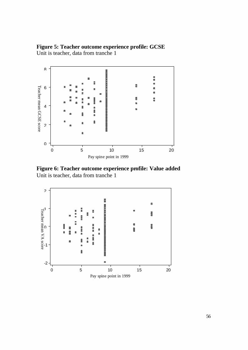
56

Figure 5: Teacher outcome experience profile: GCSE Unit is teacher, data from tranche 1

0

2

4

6

8

Teacher m

ean GC

SE score

0 5 10 15 20

Pay spine point in 1999

Figure 6: Teacher outcome experience profile: Value added Unit is teacher, data from tranche 1

-2

-1

0

1

2

Teacher m

ean VA

score

0 5 10 15 20 Pay spine point in 1999

57

Appendix 1: Data collection Schools were approached in several waves, between June 2000 and January 2002. The first wave comprised a pilot group of 40 schools, chosen from a group of about 200 schools who had previously participated in a Department for Education and Skills (DfES, then DfEE) pilot value-added exercise (O’Donogue et al 1997). These schools were therefore known to be research aware and to have good information systems. We selected the 40 schools as a convenience sample of the schools closest to Bristol. The second wave comprised the remaining schools from the DfEE pilot group. Third and subsequent waves comprised schools in particular groups of LEAs, chosen to reflect a balance of school types and urban/rural features. Schools were approached by being sent a letter inviting them to participate, as well as a project outline and a stamped-addressed postcard to return indicating whether they were / were not willing to participate, or wanted more information before taking a decision. Their addresses were obtained from the DfES Performance Tables. Schools in the first wave were all telephoned after the initial, letter-based approach. Schools in the first and second waves who did not respond to the initial approach were sent a follow-up letter and subsequently telephoned. The phone calls were extremely time consuming (up to eight calls had to be made to each school to speak to the head, or to draw the issue to the head’s attention), and only a small number of schools agreed to participate as a result. Intensive follow-up was therefore dropped from subsequent waves, in favour of more extensive sampling. Given the poor response rate from our initial waves and the expected high drop-out rate, we invited all state maintained secondary schools in England to take part. After agreeing to participate, schools were sent a letter guaranteeing the confidentiality and security of the data and a schedule of the data required for Tranche 1 (1997 – 1999). To obtain additional supplementary information the headteachers of participating schools were interviewed or were asked to fill in a questionnaire (see Croxson and Atkinson (2001a, b) for more on these interviews). Participating schools were then sent a second data schedule in the Autumn of 2002, which specified the data required for Tranche 2 (2000 - 2002). A copy of this schedule is shown in Table A1. 41 schools provided Tranche 1 data, of whom 24 also provided data for Tranche 2. Out of this number, the data supplied by 18 schools was sufficiently complete for our analyses.

58

Table A1: General schedule of data requirements for pupils taking GCSEs in Summer 2002 Examples

Class lists for

Year 10: 2000/2001, Year 11: 2001/2002 All Maths, English and Science subjects

Names of pupils linked to the appropriate teachers for each of the 2 years (if classes remain the same across years do not duplicate the info) Subject Setting information (ie which group is highest ability, etc. if relevant)

Class: 10A (00/01) Maths; Class: 11G Teachers: Mr Smith & Ms Jones Teachers: A Rig Pupils: Jo Dean, Bob Aasive, Pupils:

and so on for each class Maths 10A High Achievers - 10G Strugglers English, no setting Science S1 Double Science, S2 – 5 Single Science

Information about these pupils • date of birth • gender; • postcode.

for each pupil

Pupil KS3 Science

GCSE Science (AQA)

Jo Dean 4 D Bob Aasive 4 C Tane Mujab 7 A* …

Test and exam information for these pupils KS3 test scores for these pupils, in each of Maths, English and Science GCSE Results and Exam Board in each of Maths, English and Science

and so on for each pupil

Teacher Date of birth Gender

Ms Jones 09/07/66 F

Mr Smith 08/04/61 M

Characteristics of the teachers who taught them

• date of birth; • gender; • subject(s) taught; • length of time at school at 1/9/01; • total salary at 1/9/00; total salary at 1/9/01; • spine point at 1/9/00; spine point at 1/9/01; • whether they were (a) eligible for; (b) applied for;

(c) awarded Threshold Payment in 2001; • whether they were (a) eligible for; (b) applied for;

(c) awarded Threshold Payment in 2002.

and so on for each teacher

Information about the school • total number of teachers in the school; full time and part time at 1/9/00 AND 1/9/01;

• number of teachers that were (a) eligible for; (b) applied for; (c) awarded a Threshold payment in 2001;

• number of teachers that were (a) eligible for; (b) applied for; (c) awarded Threshold payment in 2002.

59

Appendix Figure 1

Tranche 2

Tranche 1

June 1997 Tranche 1 take KS3

Sept 1997 Tranche 1 start GCSEs

June 1998

June 1999 Tranche 1 take GCSEs

June 2000 Tranche 2 take KS3

Sept 2000 Tranche 2 start GCSEs

June 2001

June 2002 Tranche 2 take GCSEs

First Performance Threshold Year

July 2000 First PT Evaluation

Sept 1999 Scheme Introduced and Eligibility Defined

Documents

Evaluating the Impact of Performance- related Pay for Teachers in