CENTRUM Católica’s Working Paper Series

No. 2012-09-0007 / September 2012

Evaluating the Performance of Indian Banking Sector

using Data Envelopment Analysis during Post-Reform

and Global Financial Crisis

Mukesh Kumar

Vincent Charles

CENTRUM Católica – Pontificia Universidad Católica del Perú

Working papers are in draft form. This working paper is distributed for purposes of comment and discussion only. It may not be reproduced without permission of the author(s).

CENTRUM Católica‟s Working Paper No. 2012-09-0007

Evaluating the performance of Indian banking sector using data envelopment

analysis during post-reform and global financial crisis

Mukesh Kumar and Vincent Charles

CENTRUM Católica, Pontificia Universidad Católica del Perú, Santiago de Surco, Perú

E-mail: mkumar@pucp.edu.pe, vcharles@pucp.pe

Enticed by the reform of Indian banking sector in the early 1990s and further slowdown in the economy as a result

of global financial crisis in late 2000s, the current study analyzes the performance of Indian banks using data

envelopment analysis. The performance is measured in terms of technical efficiency, returns-to-scale, and

Malmquist productivity index for a sample of 33 banks, consisting of 19 public sector and 14 private sector banks

during the period spanning 1995-96 to 2009-10. The jackknifing analysis, followed by the dummy variable

regression model is used to identify the outlier and its possible impact on overall efficiency trends. Findings reveal

that efficiency scores are robust in the sense that the inclusion of outlier does not affect the overall efficiency trends.

The public sector bank is faintly doing better than the private sector banks in terms of (i) technical efficiency since

2003-04 and (ii) scale efficiency from 2000-01 onwards. There is growing tendency of public banks operating under

increasing returns to scale, implying that substantial gains could be obtained from altering scale via either internal

growth or consolidation in the sector. The difference in the Total Factor Productivity (TFP) change between these

two types of banks is found to be statistically significant in favour of public sector banks. The technological change

has been the dominating source of productivity growth, whereas, the contribution of pure efficiency change and

scale change are found to be negligible in Indian banking sector during the period of study. The reform in Indian

banking sector has clearly re-energized the Indian banking sector as a whole, resulting in a positive change in TFP

through technological change possibly as a result of adoption of latest technology and new business practices in post

reform period. However, there is evidence of shrink in the market resulting in movement of the banks towards

increasing returns-to-scale as well as negative growth in TFP in both the sectors during the period of global financial

crisis.

Keywords: Data envelopment analysis; Indian banking sector reform; global financial crisis; technical efficiency;

returns-to-scale; Malmquist productivity index; Jackknifing analysis

Introduction

A sound financial system is crucial for an indispensable and vibrant economy. Thus, the performance of

any economy to a large extent is dependent on the performance of the banking sector as it being the

predominant component of the financial service industry. The Indian banking sector went through

structural changes since its independence keeping in view its financial linkages with the rest of the

economy and to meet the social and economic objectives of development (Kumbhakar and Sarkar, 2005).

Consequently, the sector was initially following strict controls on interest rates, as well as stringent

regulations relating to branch licensing, directed credit programs, and mergers. However, the closed and

strict regulated environment started showing adverse affect on the sector, resulting in under-performance

of the banks over the years. As a result, Indian banking sector underwent a sea of changes through its

liberalization policy in early 1990s with implementation of a series of reforms with an objective to make

the banking sector more productive and efficient by limiting the state intervention and enhancing the role

of market forces.

Like most developing countries, the banking sector in India is characterized by the co-existence of

different ownership groups, public and private, and within private, domestic and foreign. The Indian

public sector banks (PSBs) came into existence in several phases. In 1955, the Government of India took

CENTRUM Católica‟s Working Paper No. 2012-09-0007

over the ownership of the Imperial Bank of India and reconstituted it as State Bank of India (SBI) under

the State Bank of India Act of 1955. Later, the State Bank of India (subsidiary banks) Act was passed in

1959 allowing SBI to take over seven banks of large states as its associate banks. However, in spite the

progress made of SBI and its subsidiaries in terms of geographic coverage and credit expansion, it was

felt that bank credits were flowing mainly to the large and well established business firms and primary

sector such as agriculture and small scale industries were almost neglected. This resulted in an

announcement of policy of social control over banks in 1969 and consequently fourteen largest private

banks were nationalized under the Nationalization Act 1969. In the second phase of nationalization,

another six private banks were nationalized in 1980. The private and foreign banks were operating side-

by-side, but on a relatively small scale and their activities were restricted through entry regulation and

strict branch licensing policies. During the period of 1969-1991, the number of banks increased slightly,

but savings were successfully mobilized in part because the number of branches held by public sector

banks was encouraged to expand rapidly. Further, relatively low inflation kept negative real deposit

interest rates at a mild level, which in turn helped the banks to increase deposits. However, many banks

remained unprofitable, inefficient, and unsound owing to their poor lending strategy and lack of internal

risk management under government ownership. The prolonged presence of excessively large PSBs

resulted in inefficient resource allocation and concentration of power in a few banks.

Facing major economic crisis, the Reserve bank of India (RBI) launched major banking sector

reforms in 1991 aimed at creating a more profitable, efficient and sound banking system, based on the

recommendations of the first Narasimham committee on financial sector reforms. The reforms sought to

improve the bank efficiency through entry regulation1, branch delicensing, deregulation of interest rate

2,

and diversifying ownership of PSBs by enabling the state-owned banks to rise up to 49 per cent of their

capital from the market. The reforms also targeted at improving bank profitability through the gradual

reduction of the Cash Reserve Ratio (CRR)3 and the Statutory Liquidity Ratio (SLR)

4, and to strengthen

the banking system by introducing the micro prudential measures5 (see Bhide et al., 2001; Reddy, 2006;

Prasad and Ghosh, 2007; and Kumar and Charles, 2011 for extensive review of the recent banking sector

reform). These reforms are expected to have an impact on the operations of banks. With reduced statutory

requirements banks will have more funds at their disposal for commercial lending and the interest rate

liberalization is expected to bring flexibility and competition into the banking system. The competition is

further infused by opening up banking sector for the private and foreign banks. Along with these

flexibilities, certain regulatory reforms are also introduced, which are meant to equip the banks to face

fluctuations in the economy.

However, the turmoil in the international financial markets of advanced economies that started

around mid-2007 has exacerbated substantially since August 2008. The first hint of the trouble came from

the collapse of two Bear Stearns hedge funds in early 2007 (Prasad and Reddy, 2009). Subsequently a

number of other banks and financial institutions also began to show signs of distress. Matters really came

to the force with the bankruptcy of Lehman Brothers, a big investment bank, in September 2008. In spite

of the fact that Indian banking system is not directly exposed to the sub-prime mortgage assets, the shock

has been felt in Indian financial market as well, since India is far more exposed to international markets

after macro-economic reforms of 1991. The financial sector, especially banks, is subject to prudential

regulations, both in regard to capital and liquidity. As the current global financial crisis has shown,

liquidity risks can increase manifold during a crisis and can pose serious downside risks to

macroeconomic and financial stability (Mohan, 2008). The RBI's policy response aimed at containing the

contagion from the outside in order to keep the domestic money and credit markets functioning normally

and see that the liquidity stress does not trigger solvency cascades (Subbarao, 2009). In particular, three

objectives6 were targeted: first, to maintain a comfortable rupee liquidity position; second, to augment

foreign exchange liquidity; and third, to maintain a policy framework that would keep credit delivery on

track so as to arrest the moderation in growth.

Given this background the current study examines (i) how far such reform measures have been

successful in their objective of improving the performance of the Indian banks during the post

liberalization period and (ii) whether the global financial crisis had any impact on the performance of

CENTRUM Católica‟s Working Paper No. 2012-09-0007

Indian banking sector. We use the technique of Data Envelopment Analysis (DEA) to examine the

performance of Indian banking sector and two major ownership structure within it in terms of technical

efficiency, returns-to-scale, and total factor productivity (TFP) change for the entire 15 years of post-

liberalization period as well as two sub-periods: (i) pre global financial crisis period (1996-2007) and (ii)

global financial crisis period (2008-2010). Within the framework of the current study, the results seem to

be conclusive. The DEA efficiency scores are found to be robust in the sense that the inclusion of outlier

bank does not affect the overall trends of efficiency in the present context. PSBs perform as par with its

counterpart private sector banks in terms of efficiency. Further, there is growing tendency of PSBs

operating under increasing-returns-to-scale (IRS), implying that substantial gains could be obtained from

altering scale via either internal growth or consolidation in the sector. Coming to the TFP change, PSBs

outperform private sector banks as a result of significant differences in technological change in sub-period

I. However, there is evidence of shrink in the market and negative growth in TFP in both the sectors in

sub-period II providing a gesture of adverse affect of global financial crisis on Indian banking sector.

The rest of the paper proceeds as follows. The next section provides the literature review and

highlights the contributions of the current study in Indian banking literature. It is followed by a section on

methodology, wherein we briefly present the DEA models for measuring efficiency, returns-to-scale and

Malmquist productivity index. Next, the paper provides the detailed description of data, followed by

results of the empirical analysis. Finally, the paper concludes with some future scope of the study.

Literature Review A number of attempts have been made to study the efficiency and productivity of banking sector in

developed countries (Berger and Humphrey, 1997; Berger et al.,1999; Isik and Hassan, 2002 a, b;

Yildirim and Philippatos, 2007). However, studies analyzing the efficiency of banks in developing

countries, including India, are relatively modest. In their extensive international literature survey, Berger

and Humphrey (1997) noted that the vast majority of the efficiency literature focuses on the banking

markets of well-developed countries with particular emphasis on the U.S. markets. Fethi and Pasiouras

(2010) provided an extensive survey on efficiency and productivity studies in banking sector published in

various research journals covering the period 1998-2008. They identified 151 studies that use DEA to

estimate various measures of bank efficiency and productivity growth, and 30 studies that provide similar

estimates at the branch level. More than 75% of the studies focus on efficiency and productivity issues of

banks in developed countries.

The literature on bank efficiency reveals mixed experiences of liberalization policies undertaken in

various countries. A number of studies report the existence of efficiency gains due to liberalization

programmes undertaken in various emerging and transition countries including Turkey (Zaim, 1995; Isik

and Hassan, 2003), Thailand (Leightner and Lovell, 1998), Hungary (Hasan and Marton, 2003), the

Central and Eastern European (CEE) transition countries (Brissimis et al., 2008), Pakistan (Ataullah and

Le, 2006), and Egypt (Fethi et al., 2011). However, there are few studies which show no improvement in

bank efficiency over the transition period such as, Havrylchyk (2006) for Polish, Kasman and Yildirim

(2006) for the CEE transition countries, Fu and Heffernan (2009) for China. Moreover, a number of

studies (Burki and Niazi, 2009; Hsiao et al., 2010) illustrate that the efficiency impact of the reform

process may not be immediately visible or uniform over time. The efficiency may go down at first due to

the initial costs of adjustment prior to improving later. Burki and Niazi (2010), for example, show that

efficiency fell during the initial reform period in Pakistan due to the adjustment process before increasing

in the later stages of the reform process. Similarly, Hsiao et al. (2010) find that the efficiency of

Taiwanese banks was lower during the restructuring reform period than pre-reform period while being

higher in the post-reform period.

In the Indian context, there are few studies which especially focused on the efficiency measurement

of PSBs using DEA. For example, Das (1997) studied technical, allocative and scale efficiency of

different PSBs for the period 1990-1996 using DEA approach. The study found decline in overall

efficiency over time, decline in technical efficiency with slight improvement in allocative efficiency. The

State bank of India was found to be more efficient than other PSBs. Saha and Ravisankar (2000) analyzed

CENTRUM Católica‟s Working Paper No. 2012-09-0007

the performance of Indian banks using DEA approach for a sample of 25 PSBs banks over a period 1992-

1995. Their findings reveal that barring few exceptions, the public sector banks have in general improved

their efficiency over the years.

Other group of studies which focused on the comparison of various categories of banks based on

ownership includes Bhattacharya et al. (1997), Sathye (2003), Sahoo et al. (2007), Sinha (2008), Mahesh

and Rajeev (2009) and Kumar and Charles (2011).

Bhattacharya et al. (1997) used DEA to measure the productive efficiency of Indian commercial

banks in the late 1980‟s to early 1990‟s and to study the impact of policy of liberalizing measures taken in

1980‟s on the performance of various categories of banks. They found that the Indian PSBs were the best

performing banks, as the banking sector was overwhelmingly dominated by the PSBs, while the new

private sector banks were yet to emerge fully in the Indian banking scenario. Sathye (2003) measured the

productive efficiency of 94 banks in India for the year 1996-1997 by using DEA wherein, they found that

the PSBs were on average more efficient than foreign banks, which in turn were more efficient than

private banks. Similarly, Gupta et al. (2008) found that the SBI and its group have the highest efficiency,

followed by private banks, and the other nationalized banks for the period 1999-2003. The results are

consistent over the period, but efficiency differences diminish over period of time. Mahesh and Rajeev

(2009) examined the changes in productive efficiency of Indian commercial banks for the post reform

period 1985-2004. They found that deregulation has significant impacts on all three types of efficiency

measures. PSBs as a group ranks first in all the three efficiency measures showing that, as opposed to the

general perception, these banks are doing better than their private counterparts. Private banks, however

have shown marked improvement during the post-liberalization period in terms of all three types of

efficiency measures.

Contrary to the above stated studies, Sahoo et al. (2007) who examined the efficiency trends of the

Indian commercial banks during the period 1997-1998 to 2004-2005 observed that foreign banks are seen

outperforming over both the nationalized banks and private banks, and private and foreign banks as a

group outperforming over the nationalized banks. Similarly, Sinha (2008) observed that the private sector

commercial banks have higher mean technical efficiency score when compared to the public sector

commercial banks and most of the commercial banks experienced decreasing-returns-to-scale (DRS)

during the study period spanning from 2002-2003 to 2004-2005.

To sum-up, most of the studies show the evidence of affirmative gesture of reform process on the

efficiency of Indian banking sector. While most of the studies provided the evidence of PSBs performing

better than its counterpart, private and foreign banks, few other studies have found the PSBs as

underperforming compared to other group of banks. The differences in the findings of various studies in

Indian context are attributed to many factors including the selection of time period, sample size, selection

of inputs and outputs variables and the orientation of efficiency measurement.

However, one of the major limitations of all the above studies is that they focused on only one aspect

of performance measurement, i.e., efficiency. Controversy is not only concerned with whether

deregulation stimulates efficiency but also on different sources of productivity growth. While some

studies attribute the growth of productivity to technological progress (Avkiran, 2000; Alam, 2001;

Mukherjee et al., 2001; Canhoto and Dermine, 2003; Kumbhakar, Lozano-Vivas, Lovell, & Hasan, 2001;

Sturm and Williams, 2004) others are in favour of efficiency improvement (Berg et al., 1992; Gilbert and

Wilson, 1998; Isik and Hassan, 2003). Compare to efficiency analysis, the literature on the issue of TFP

growth in Indian banking sector is very limited. Galagedera and Edirisuriya (2005) investigated the

efficiency and productivity for a sample of Indian commercial banks over the period 1995-2002 by using

the technique of DEA. The results reveal that there has been no significant growth in productivity during

the study period. When analyzed separately, the PSBs reveal a modest growth in productivity that appears

to have been brought about by technological change. The private sector banks indicate no growth. Zhao

et al. (2008) used balanced panel data set covering the period 1992-2004 to measure DEA-based

Malmquist index of TFP change in Indian banking sector. The results revealed that after an initial

adjustment phase of deregulation period, the Indian banking sector experienced sustained productivity

growth, driven mainly by technological progress. Bank‟s ownership structure seems to have an impact on

CENTRUM Católica‟s Working Paper No. 2012-09-0007

bank efficiency but doesn‟t appear to have an influence of TFP change. Kumar et al. (2010) observed that

TFP growth for Indian banking sector for the period of 1995-2006 was driven mainly by technological

progress as compared to efficiency change.

The current study contributes to the literature significantly in many ways. Most of the literature in

Indian banking sector focused on measurement of efficiency (e.g., Das, 1997; Saha and Ravishankar,

2000; Sathye, 2003; Ram Mohan & Ray, 2003; Sahoo et al., 2007) and a few studies on benchmarking

(e.g., Gupta et al., 2008; Kumar and Charles, 2011). A detailed systematic study on the measurement of

productivity change in Indian banking sector is comparatively limited. Along with the issue of efficiency

and returns-to-scale, we also use a broad dynamic indicator, TFP change index, as the measure of

performance. It is an important tool for reviewing past growth patterns and for assessing the potential for

future growth. Ahluwalia and Shanker (1985) pointed out that one needs to look at the concept of TFP to

evaluate the performance of the service sector in India, which not merely reflects productive efficiency of

inputs but also the capacity of the management to combine these and other factors to enhance the outputs

of the firm.

Secondly, in comparison to previous studies (e.g., Galagedera and Edirisuriya, 2005; Sinha, 2008;

Zhao et al., 2008), this study considers more recent data for a relatively longer period of latest 15 years of

post-liberalization which includes 3 years of global financial crisis period. There has been debate among

the policy makers, bankers and researchers since the mid of 2007 whether the global financial crisis had

any impact on the performance of India banking sector. It is believed that Indian banking sector is

unlikely to get affected with global financial crisis as (i) the banking system in India has had no direct

exposure to the sub-prime mortgage assets or to the failed institutions. It has very limited off-balance

sheet activities or securitized assets (ii) India's recent growth has been driven predominantly by domestic

consumption and domestic investment with very limited reliance of external demand. Other contrary view

is that with the increasing integration of the Indian economy and its financial markets with rest of the

world, there is possibility that the country does face some downside risks from these international

developments. However, no attempt has been made till date to empirically resolve this debate. The current

paper compares the performance of Indian banks before and after the global financial crisis.

Thirdly, most of the previous studies in the Indian context decompose the Malmquist productivity

index into its different components by using the extended decomposition model proposed by Färe et al.

(1994). The extended model of Färe et al. (1994) assumes constant-returns-to-scale (CRS) at the stage of

measuring technological change but subsequently switches to variable-returns-to-scale (VRS) to separate

the scale effect component, which is not internally consistent. Hence, the current study uses the

decomposition model developed by Ray and Desli (1997) that assumes VRS to measure each and every

component of Malmquist productivity index.

Finally, DEA is a computationally convenient way to measure efficiency that does not require an

explicit functional relationship between inputs and outputs. However, because the frontier is constructed

using extreme observations, DEA can be sensitive to extreme points, especially when data may be

contaminated by measurement error. In such settings, the technical efficiency scores calculated from

datasets that include outliers can be misleading. In spite of this limitation, most of previous studies did not

give much attention to verify the robustness of the DEA efficiency scores. The current paper diagnoses

the robustness of efficiency scores obtained through DEA by using Jackknifing analysis. Further, the

sensitivity of outlier on overall efficiency trends is tested through dummy variable regression models.

Methodology The stochastic frontier (parametric) model and DEA (non-parametric) model emerged as two alternative

developments of ideas that originated with Farrell (1957). Grosskopf (1986) noted that the parametric

approach has been developed mainly by economists, whereas, nonparametric has been left to those in

operations research. The choice of a non-parametric approach in the current study is based on several

considerations. Firstly, when using panel data parametric approaches often use a time trend, which

smoothes the variation of productivity changes over time. By contrast, non-parametric approaches allow

for substantial variations embedded in data to be revealed (Alam, 2001). Secondly, in the parametric

CENTRUM Católica‟s Working Paper No. 2012-09-0007

approach, the decomposition of error term into two parts, one representing stochastic error and the other

inefficiency is not useful for the data sets of fewer than one hundred observations (Aigner et al., 1977). In

contrast, DEA works well with a small sample size. Thirdly, the incomplete knowledge of the statistical

properties of the estimates and restrictiveness of reference technology affects the bias of the estimates in

parametric model. Grosskopf (1986) pointed out that both the degree of restrictiveness of the reference

technology as well as choice of error structure greatly affects the values of efficiency. In contrast, DEA

does not require any underlying assumption of a functional form relating to inputs and outputs. Given the

set of inputs and outputs of different firms, it constructs its own functional form, thus avoiding the danger

of miss-specification of the frontier. Also, it does not make the assumption that all decision making units

(DMUs) are using the same technology, but instead evaluates the efficiency of DMU relative to its peer or

combination of peers. Further, DEA readily incorporates the existence of multiple outputs. However, a

major drawback of DEA is its inability to detect measurement error. Thus, an exceptionally well

performing unit (outlier) may seriously compromise the analysis.

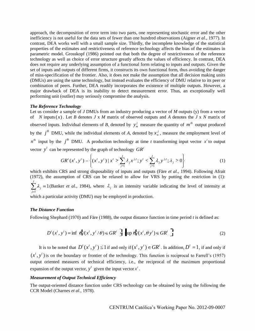
The Reference Technology

Let us consider a sample of J DMUs from an industry producing a vector of M outputs (y) from a vector

of N inputs )(x . Let B denotes J x M matrix of observed outputs and A denotes the J x N matrix of

observed inputs. Individual elements of B, denoted by j

my measure the quantity of thm output produced

by the thj DMU, while the individual elements of A, denoted by

j

nx , measure the employment level of

thn input by the thj DMU. A production technology at time t transforming input vector

tx to output

vector ty can be represented by the graph of technology

tGR

J

j

j

tj

j

tJ

j

tj

j

tttttt yyxxyxyxGR1

,

1

, 0;;|),(),(

(1)

which exhibits CRS and strong disposability of inputs and outputs (Färe et al., 1994). Following Afrait

(1972), the assumption of CRS can be relaxed to allow for VRS by putting the restriction in (1): J

j

j

1

1(Banker et al., 1984), where j is an intensity variable indicating the level of intensity at

which a particular activity (DMU) may be employed in production.

The Distance Function

Following Shephard (1970) and Färe (1988), the output distance function in time period t is defined as:

1),/(sup)/,/(inf),( ttttttttt GRyxGRyxyxD (2)

It is to be noted that 1),( ttt yxD if and only ifttt GRyx ),( . In addition, 1tD , if and only if

),( tt yx is on the boundary or frontier of the technology. This function is reciprocal to Farrell‟s (1957)

output oriented measures of technical efficiency, i.e., the reciprocal of the maximum proportional

expansion of the output vector,ty given the input vector

tx .

Measurement of Output Technical Efficiency

The output-oriented distance function under CRS technology can be obtained by using the following the

CCR Model (Charnes et al., 1978).

CENTRUM Católica‟s Working Paper No. 2012-09-0007

Model I: Output-oriented single-period distance function under CRS (CCR Model)

.,0;;..

,

1

,',',

1

,',

,'1,','

jyyxxts

MaxyxD

j

J

j

tj

m

tj

c

tj

mj

J

j

tj

n

tj

nj

tj

c

tjtjt

c

(3)

The output-oriented single period distance function measures the maximum proportional change in

outputs required to make ),( tt yx feasible in relation to the technology at time period t. In other words,

the efficiency of DMU in time period t is evaluated with reference to the technology in the same time

period t. The output distance function under VRS technology can be obtained by adding additional

convexity constraintJ

j

j

1

1 in CCR model, popularly known as BCC model (Banker et al., 1984).

Model II: Output-oriented single period distance function under VRS (BCC Model)

.,0;1; ;..

,

11

,',',

1

,',

,'1,','

jyyxxts

MaxyxD

j

J

j

j

J

j

tj

m

tj

v

tj

mj

J

j

tj

n

tj

nj

tj

v

tjtjt

v

(4)

Measurement of Returns to Scale

Decomposing technical efficiency (TE) into pure efficiency (PE) and scale efficiency (SE) allows an

insight into the sources of inefficiencies. It also helps to determine whether banks operate under optimal

or non-optimal returns-to-scale. The CRS efficiency score obtained from the Model I represents technical

efficiency, which measures inefficiencies due to the input/output configuration and as well as the size of

operations. On the other hand, the VRS efficiency score obtained from the Model II represents pure

efficiency, that is, a measure of efficiency without scale efficiency. The scale efficiency can be obtained

as the ratio of technical efficiency to pure efficiency.

Once the scale efficiency scores are computed, the analysis can be taken a step further. This involves

determining whether a particular DMU is experiencing the optimal scale, operating under CRS or non-

optimal returns-to-scale, either operating under IRS or DRS. To make this assessment, DEA is repeated

with non-increasing returns-to-scale (NIRS) by incorporating the restriction J

j

j

1

1 in the Model I. If

the score for a DMU under VRS equals the NIRS score, it implies that DMU operates under DRS. If not;

it implies that DMU operates under IRS (Coelli et al., 1998). If the VRS score equals the CRS score, then

the DMU is said to be operating at the optimal scale or the most productive scale size.

Measurement of Malmquist Productivity Index

To define a Malmquist productivity index, let us define the distance functions with respect to two

different time periods as follows:

111111 )/,/(inf),( and )/,/(inf),( tttttt

o

tttttt

o SyxyxDSyxyxD (5)

CENTRUM Católica‟s Working Paper No. 2012-09-0007

where „o‟ indicates that the distance function is output-orientated. The first mixed-period distance

function in (5) measures the maximum proportional change in outputs required to make ),( 11 tt yx

feasible in relation to the technology at time period t. Similarly, the second mixed-period distance

function in (5) measures the maximum proportional change in outputs required to make ),( tt yx feasible

in relation to the technology at time period t+1. In both these mixed-period cases, the value of the

distance function may exceed unity if the observation being evaluated is not feasible in the other period.

Following Ray and Desli (1997), the Malmquist productivity index can be defined as:

2

1111112

1

1

11111

0),(

),(

),(

),(

),(

),(

),(

),(ttt

ttt

ttt

ttt

ttt

v

ttt

v

ttt

v

ttt

v

yxSE

yxSE

yxSE

yxSE

yxD

yxD

yxD

yxDM (6)

The first component of (6) can further decomposed as:

),(

),(

),(

),(

),(

),( 1112

1

111

11

1 ttt

v

ttt

v

ttt

v

ttt

v

ttt

v

ttt

v

yxD

yxD

yxD

yxD

yxD

yxD (7)

where the first component of (7) is the geometric mean of two ratios, which measures the shift in the

technology calculated at tx and

1tx . The second component measures the change in relative efficiency

between the years t and 1t . The second component of (6) which involves both CRS and VRS distance

functions at both the time periods, measures the change in scale efficiency. Thus, Malmquist productivity

index is the product of technological change, pure efficiency change and scale efficiency change.

The single-period distance functions under the CRS and VRS are solved using Model I and II

respectively; whereas the mixed-period distance functions under CRS are solved using Model III and IV

(see Appendix A). The mixed-period distance functions under the VRS are solved using Model III and IV

with the restriction on sum of intensity variables, i.e.,J

j

j

1

1 .

The Database Selection of Inputs and Outputs and Purification of Data

There is on-going discussion in the banking literature regarding the proper definition of inputs and

outputs (Fethi and Pasiouras, 2010). Till today, there is no all-encompassing theory of the banking firm

and no agreement on the explicit definition and measurement of banks' inputs and outputs (Casu, 2002;

Sathye, 2003). Two different approaches appear in the literature regarding the measurement of inputs and

outputs of a bank, popularly known as production approach and intermediation approach (Humphrey,

1985). The production approach views banks as using purchased inputs to produce deposits and various

categories of bank assets. Both loans and deposits are, therefore, treated as outputs and measured in terms

of the number of accounts. This approach considers only operating costs and excludes the interest

expenses paid on deposits since deposits are viewed as outputs. The intermediation approach on the other

hand considers banks as financial intermediaries and uses volume of deposits, loans and other variables as

inputs and outputs. It views the banks as using deposits together with purchased inputs to produce various

categories of bank assets. Outputs are measured in monetary values and total costs include all operating

and interest expenses7.

Following Berger and Humphrey (1997), we have used intermediation approach8 with restricted

choice of variables9. As the number of variables increases in DEA analysis, the ability of the model to

discriminate among the DMUs decreases. The more variables are added the greater becomes the chance

that some inefficient unit dominates in the added dimension and becomes efficient (Smith, 1997). In order

to preserve the discriminatory power of DEA, the number of inputs and outputs should be kept at a

reasonable level. The choice of the inputs and outputs are guided by the choices made in previous studies

CENTRUM Católica‟s Working Paper No. 2012-09-0007

and also on the data availability. In the current study, we have used two inputs – total cost10

and total

deposits. The input total cost is measured as the sum of total interest expenses and non-interest expenses

including personal expenses. Non-interest expenses include service charges and commissions, expenses

of general management affairs, salaries, and other expenses (including health insurance and securities

portfolios). Some researchers (Yeh, 1996; Sathye, 2003; Ram Mohan and Ray, 2004; Kao and Liu, 2004)

have treated interest expenses and non-interest expenses as two different inputs along with other inputs.

However, following Casu and Molyneux (2003) and Sealey and Lindley (1977), we have treated both

together as a single input as total cost. This kind of treatment is mainly due to the well-known

dimensionality problem associated with DEA particularly with limited sample size: a high number of

variables relative to the number of observations cause more units to be wrongly identified as efficient

(Zhao et al., 2008). The input, total deposit is taken as the sum of demand and savings deposits held by

bank and non-bank depositors.

The above two inputs are used to produce two outputs namely, total loans and other earning assets.

The output, total loan is measured as the sum of all loan accounts intermediated by banks and the output,

other earning assets is measured as the sum of total securities (treasury bills, government bonds and other

securities), deposits with banks and equity investments.

To ensure the validity of the DEA model specification, an isotonicity test (Avkiran, 1999) was

conducted, which involves the calculation of all inter-correlations between inputs and outputs for

identifying whether increasing amounts of inputs lead to greater outputs. The inter-correlation between

inputs and outputs were observed positive (Pearson correlations > 0.80; α = 0.01), the isotonicity test was

passed and the inclusion of inputs/outputs was justified. The summary statistics of inputs and outputs is

available from the author on request.

4.2 Sources of Data, Selection of time-period and Sample Size

The basic data on inputs and outputs has been taken from the electronic database, PROWESS provided by

Centre for Monitoring Indian Economy (CMIE), Pvt. Ltd. Mumbai for the period spanning 1995-1996 to

2009-2010. The CMIE, established in 1976 is the most accomplished corporate database in India and

contains a highly normalized data on time-series built on a sound understanding of disclosures in India on

over 17000 companies from different sectors. The CMIE has been proven the most conveniently and

widely used source of database for the researchers for conducting the empirical studies at firm-level in the

manufacturing sector (Kumar and Charles, 2009; Ram Mohan, 2005; Kumar and Basu, 2004) as well as

service sector (Kumar and Charles, 2011; Udayakumar et al., 2011; Ghosh, 2009; Debasish, 2006; Ram

Mohan, 2005; Saha and Ravisankar, 2000). The sample consists of commercial banks including both

public and private banks for which the data were available for the entire period 1995-1996 to 2009-2010.

The commercial banking is the most important part of modern banking set up in India. Today, the

commercial banks are having their branches all over India including the rural areas and their functions are

confined not only to advancing loans to the public and accepting their deposits, but they also play

significant role in accelerating the rate of economic development and fulfilment of various socio

economic objectives of the Government. The total number of branches of all schedules commercial banks

is 79735 with approximately 40% of their branches located in rural areas, followed by 24%, 19% and

17% respectively located in semi-urban, urban and metropolitan cities (Government of India, 2010).

There were 35 commercial banks in total for which the data were available during the study period.

However, one of the private banks, Kotak Mahindra Bank Ltd. was dropped from the sample because of

excessive missing data. Another private bank, i.e., ICICI Bank Ltd. was dropped from the sample as it did

not fit into any of the broad cluster during the screening of the data. Nunamaker (1985) and Raab and

Lichty (2002) suggested a rule of thumb on deciding the minimum size of the sample in any DEA study.

The sample size should be at least three times larger than the sum of the number of inputs and outputs. In

our study, with a total of two inputs and two outputs, we ended up with a reasonably good sample size of

33 banks (see Appendix B) consisting of 19 public banks and 14 private banks. All the public sector

banks in the sample are nationalized banks. In May 2008, Centurion Bank of Punjab Ltd. (CBPL) merged

CENTRUM Católica‟s Working Paper No. 2012-09-0007

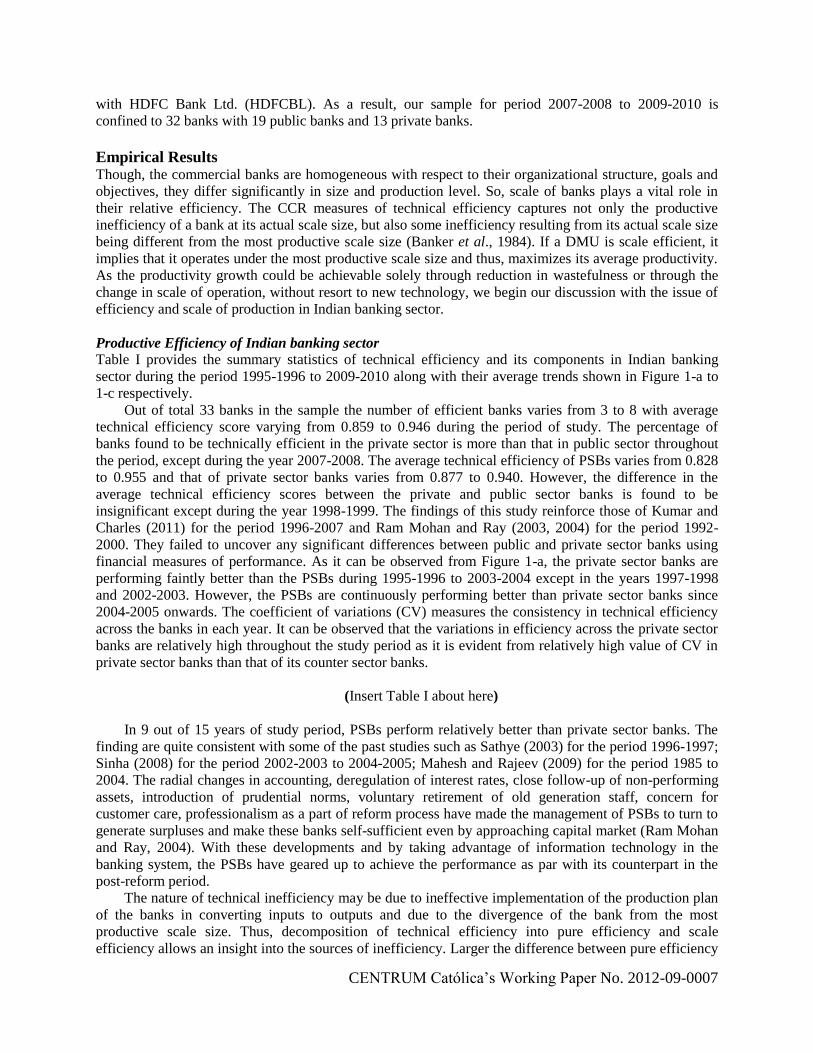
with HDFC Bank Ltd. (HDFCBL). As a result, our sample for period 2007-2008 to 2009-2010 is

confined to 32 banks with 19 public banks and 13 private banks.

Empirical Results Though, the commercial banks are homogeneous with respect to their organizational structure, goals and

objectives, they differ significantly in size and production level. So, scale of banks plays a vital role in

their relative efficiency. The CCR measures of technical efficiency captures not only the productive

inefficiency of a bank at its actual scale size, but also some inefficiency resulting from its actual scale size

being different from the most productive scale size (Banker et al., 1984). If a DMU is scale efficient, it

implies that it operates under the most productive scale size and thus, maximizes its average productivity.

As the productivity growth could be achievable solely through reduction in wastefulness or through the

change in scale of operation, without resort to new technology, we begin our discussion with the issue of

efficiency and scale of production in Indian banking sector.

Productive Efficiency of Indian banking sector

Table I provides the summary statistics of technical efficiency and its components in Indian banking

sector during the period 1995-1996 to 2009-2010 along with their average trends shown in Figure 1-a to

1-c respectively.

Out of total 33 banks in the sample the number of efficient banks varies from 3 to 8 with average

technical efficiency score varying from 0.859 to 0.946 during the period of study. The percentage of

banks found to be technically efficient in the private sector is more than that in public sector throughout

the period, except during the year 2007-2008. The average technical efficiency of PSBs varies from 0.828

to 0.955 and that of private sector banks varies from 0.877 to 0.940. However, the difference in the

average technical efficiency scores between the private and public sector banks is found to be

insignificant except during the year 1998-1999. The findings of this study reinforce those of Kumar and

Charles (2011) for the period 1996-2007 and Ram Mohan and Ray (2003, 2004) for the period 1992-

2000. They failed to uncover any significant differences between public and private sector banks using

financial measures of performance. As it can be observed from Figure 1-a, the private sector banks are

performing faintly better than the PSBs during 1995-1996 to 2003-2004 except in the years 1997-1998

and 2002-2003. However, the PSBs are continuously performing better than private sector banks since

2004-2005 onwards. The coefficient of variations (CV) measures the consistency in technical efficiency

across the banks in each year. It can be observed that the variations in efficiency across the private sector

banks are relatively high throughout the study period as it is evident from relatively high value of CV in

private sector banks than that of its counter sector banks.

(Insert Table I about here)

In 9 out of 15 years of study period, PSBs perform relatively better than private sector banks. The

finding are quite consistent with some of the past studies such as Sathye (2003) for the period 1996-1997;

Sinha (2008) for the period 2002-2003 to 2004-2005; Mahesh and Rajeev (2009) for the period 1985 to

2004. The radial changes in accounting, deregulation of interest rates, close follow-up of non-performing

assets, introduction of prudential norms, voluntary retirement of old generation staff, concern for

customer care, professionalism as a part of reform process have made the management of PSBs to turn to

generate surpluses and make these banks self-sufficient even by approaching capital market (Ram Mohan

and Ray, 2004). With these developments and by taking advantage of information technology in the

banking system, the PSBs have geared up to achieve the performance as par with its counterpart in the

post-reform period.

The nature of technical inefficiency may be due to ineffective implementation of the production plan

of the banks in converting inputs to outputs and due to the divergence of the bank from the most

productive scale size. Thus, decomposition of technical efficiency into pure efficiency and scale

efficiency allows an insight into the sources of inefficiency. Larger the difference between pure efficiency

CENTRUM Católica‟s Working Paper No. 2012-09-0007

and technical efficiency, more scale inefficient a bank is, which in turn, indicates the larger deviation of

the bank from the most productive scale size. On the other hand, as pure efficiency approaches technical

efficiency, the bank approaches to the most productive scale size and a bank becomes scale efficient as

pure efficiency equals technical efficiency.

On an average, the number of pure efficient banks under VRS varies from 7 to 16 with average pure

efficiency score varying from 0.917 to 0.961. The average pure efficiency score of public and private

sector banks varies from 0.905 to 0.970 and 0.920 to 0.976 respectively. The PSBs has surpassed the

private sector banks in terms of pure efficiency till 1998-99. However, the reverse is true since 2000-2001

onwards except for the years 2002-2003 and 2005-2006. However, the average pure efficiency score does

not differ significantly between two types of banks except for the year 1997-1998.

The number of banks that are scale efficient varies from 3 to 8 out of total 33 banks in the sample

with average scale efficiency score varying from 0.915 to 0.984. The average scale efficiency score of

PSBs varies from 0.914 to 0.994 and that of private sector banks varies from 0.942 to 0.988. The

difference in the average scale efficiency is found to be statistically significant between public and private

sector banks during 1998-1999, 1999-2000, 2004-2005 and 2006-2007. On an average, the private sector

banks are performing better than the PSBs in terms of scale efficiency till 2000-2001. However, the

scenario is just the reverse since 2001-2002 onwards.

(Insert Table II here)

Table II reports the average technical efficiency and its sources for each individual bank for the entire

post-reform period (1996-2010) as well as two sub-periods: (i) Pre-Global Financial Crisis Period (1996-

2007) and (ii) Global Financial Crisis Period (2008-2010). The HDFC Bank Ltd. is the only bank which

is technically efficient in sub-period I. The next most efficient bank is found to be Bank of India, followed

by State Bank of India during the entire period of study. Though, they failed to become efficient

throughout the sup-period I, they are the only banks which are technical as well scale efficient in sup-

period II. It is worth noting that in spite of global financial crisis, both public as well as private sector

banks are performing better in terms of technical efficiency in sub-period II and it continues to show

increasing trends. However, it will be misleading to conclude at this stage that Indian banking sector has

been operating completely under the clear sky during the global financial crisis period. It could be vital to

address the issue through other performance measures such as returns-to-scale and mixed period

Malmquist productivity index before we arrive at any definite conclusion.

Robustness of efficiency scores: sensitivity analysis To test the robustness of the DEA results with regards to outliers, we have applied the jackknifing

procedure wherein we ran DEA that drops out each efficient bank one at a time from analysis. Unlike

Bonesronning and Rattso (1994) who dropped each unit once at a time, we have dropped only the

efficient units that construct the frontier (Mostafa, 2010; Charles et al., 2011). The similarity of mean

efficiency between the model with all the banks included and those based on dropping out each efficient

bank one at a time has been tested by One-way ANOVA. The null hypothesis that “the removal of an

efficient bank from the sample of banks under study does not affect its mean efficiency” has been tested

for each year under study.

(Insert Table III and Table IV about here)

The results of hypotheses tests are reported in Table III. It can be observed that the null hypothesis is

accepted in all the years except during 1997, 1999, 2004 and 2005 under CRS and during 2004 and 2005

under VRS. Post-hoc analysis revealed that the mean efficiency score is sensitive only to DMU 15 in the

above stated years. Next, we examine how far the inclusion of DMU15 during the above years affects the

overall efficiency trends of Indian banking sector. In order to test whether there is any significant

CENTRUM Católica‟s Working Paper No. 2012-09-0007

difference in the slope and intercept of the trends before and after the removal of DMU 15, we have used

the following dummy variable regression model:

iiii etDtDy '

22

'

11 (8)

where, yi is the average efficiency score as the dependent variable, t is time as an independent variable

and ei is the stochastic disturbance term which is assumed to satisfy all the usual assumptions of least

square estimates. Di = 1 for trend I (with inclusion of DMU 15 in the sample during the sensitive years)

and Di = 0 for trend II (without the inclusion of DMU 15 in the sample during the sensitive years). In the

above model, α1 and α2 are the coefficients of trend II and (α1+ α'1) and (α2+ α'2) are the coefficients of trend

I. α'1 and α'2 are the differential coefficients, showing the effect of DMU 15 on the trend line. In order to

test the significance of coefficients of variables in trend I, we fit the following model:

iiii etDtDy )1()1( '

22

'

11 (9)

.2,1);(and)(where, '' kkkkkkk The trend lines before and after the removal of

DMU 15 are shown in Appendix C for technical efficiency as well as its two components, namely pure

efficiency and scale efficiency. As it can be observed from Table IV that the differential coefficients,

intercept and slope of the trends are insignificant in all the three cases. This indicates that the inclusion of

DMU 15 does not affect the overall trends in spite of it being an outlier in the present context.

The Returns to Scale in Indian Banking Sector

The presence of scale inefficiency in a bank indicates that it does not operate under the optimal scale and

thus, efficiency gains could be achieved by either expanding the production level for a bank operating

under IRS or contracting the production level for a bank operating under DRS. Table V reports the

summary statistics of returns to scale in Indian banking sector during the period 1995-1996 to 2009-2010.

As it appears from the Table V, most of the banks operate at non-optimal scale (IRS or DRS). Only 9% to

33% of banks in the sample operate under optimal scale. It is worth noting that the number of banks that

operate under DRS declines over a period of time and banks that operate under IRS increases over a

period of time.

(Insert Table V about here)

The percentage of banks that operate at optimal scale is higher in the private sector than its

counterpart throughout except during the year 2005-2006, 2007-2008 and 2008-2009. Most of the banks

in the public sector operate at DRS. On the other hand, majority of the banks in the private sector operate

at IRS. The finding is well supported with the study of Zhao et al. (2008) who found that a substantial

proportion of PSBs remain characterized by DRS, whereas, two-third of foreign and private banks operate

under IRS and optimal returns-to-scale during the period 1992-2004. Figure 1-d to 1-f shows the

percentage of banks operating under optimal, decreasing and increasing returns-to-scale respectively

during the period 1995-1996 to 2009-2010. One can observe from Figure 1-e that (i) the percentage of

PSBs operating under DRS is substantially higher than that of private sector banks at any point of time

(ii) on an average, percentage of banks operating under DRS declines over a period of time for both the

sectors. Similarly, it can be observed from Figure 1-f that (i) the percentage of PSBs operating under IRS

is substantially higher than that of private sector banks and (ii) on an average, percentage of banks

operating under IRS increases over a period of time for both the sectors. There is sharp decline (increase)

in number of banks operating under DRS (IRS) in 2007-08 possibly because of shrink in the market as a

result of global financial crisis.

CENTRUM Católica‟s Working Paper No. 2012-09-0007

Sources of TFP Change in Indian banking sector

The Malmquist productivity index can be decomposed into (i) technological change indicating how much

benchmark production frontier shifts at each bank‟s observed input mix (innovation or shocks), (ii) pure

efficiency change indicating how much closer a bank gets to the efficient frontier and (iii) scale efficiency

change indicating how much closer the banks are moving towards the most productive scale size. Table

VI reports the summary of Malmquist productivity index and its components for the entire period as well

as two sub-periods and their trends over the years are shown in Figure 1-g to 1-j.

(Insert Table VI about here)

The average annual change of TFP in Indian banking sector is observed as 1.27% during the post-

reform period, with an average annual change of 1.68% and 0.72% in public and private sector banks

respectively. The difference in the TFP change between these two types of banks is found to be

statistically significant. When we look at the contributions of different components towards TFP change,

we observe that the technological change has been the dominating source of productivity growth in Indian

baking sector during the post reform period with average annual technological change for all banks,

public banks and private banks as 1.16%, 1.49% and 0.70% respectively. On an average, the contribution

of both pure efficiency change as well as scale efficiency change is found to be negligible for the entire

period in both the sectors. During the entire 15 years of post liberalization period, the bank that achieves

the highest change in TFP is Union Bank of India with average annual change of 4.20%. This is followed

by Corporation Bank (3.91%), Uco Bank (2.87%), Canara Bank (2.84%), ING Vysya Bank Ltd. (2.82%)

and Syndicate Bank (2.63%) just to name few. In all the above banks, technological change is found to be

the dominating source of productivity change. The banks that suffer loss during the entire period of study

are Karnataka Bank Ltd. (-0.64%), Indian Bank (-0.48%), Bank of Maharashtra (-0.46%), State Bank of

India (-0.33), City Union Bank Ltd. (-0.10%) and Dena Bank (-0.08%). The technological regress is

found to be the cause of loss in TFP in Karnataka Bank Ltd, Indian Bank and State Bank of India. On the

other hand, the pure efficiency change in the case of Bank of Maharashtra and Dena Bank and the scale

efficiency change in the case of City Union Bank Ltd. are the main cause of negative growth in their TFP.

On an average, Indian banking sector has achieved a positive growth of 1.76% in pre-global financial

crisis period with an average annual growth of 2.14% and 1.24% respectively in public and private sector

banks. Most of the banks experience positive average annual change in TFP except for few exceptions

such as Bank of Rajasthan Ltd. (-1.43%), State Bank of India (-0.67%), Karnataka Bank Ltd. (-0.57%),

Development Credit Bank Ltd. (-0.45%), Indian Bank (-0.39%) and Bank of Maharashtra (-0.31%). The

technological regress was observed to be the major cause of decline in TFP for Bank of Rajasthan Ltd.,

State Bank of India and Karnataka Bank Ltd. On the other hand, loss in pure efficiency in Bank of

Maharashtra and negative change in scale efficiency in Development Credit Bank Ltd. was the cause of

negative average annual change in their TFP.

However, the scenario in the global financial crisis period, as expected is somewhat discouraging.

On an average, banks suffer loss in TFP by 0.55% with an average annual loss of 0.01% and 1.33%

respectively in public and private sector banks. The banks which manage to sustain the positive change in

TFP are Indusind Bank Ltd., Allahabad Bank, Canara Bank, Dhanalakshmi Bank Ltd., Federal Bank Ltd.,

State Bank of Bikaner & Jaipur, Syndicate Bank, Uco Bank, and Union Bank of India. The source of

positive change in TFP for these banks during global financial crisis period is basically due to pure

efficiency change, except for Development Credit Bank Ltd. and Dhanalakshmi Bank Ltd., which

achieves the gain in TFP through the scale efficiency change.

In contrast with the findings of Ram Mohan and Ray (2004) for the period 1992-2000 who could not

ascertain the proposition that productivity is lower in PSBs relative to their peers in the private sector, our

study shows significant difference in favour of PSBs mainly as a result of technological change. This is

quite consistence with the findings of Galagedera and Edirisuriya (2005) for the period 1995-2002,

Kumar et al. (2010) for the period 1995-2006; Zhao et al. (2008) for the period 1992-2004 and Heffernan

CENTRUM Católica‟s Working Paper No. 2012-09-0007

and Fu (2010) for the period 2000-2007, Mahesh and Rajeev (2009) for the period 1985-2004. They

observed that TFP change in Indian banking sector is largely driven by technological progress/innovation.

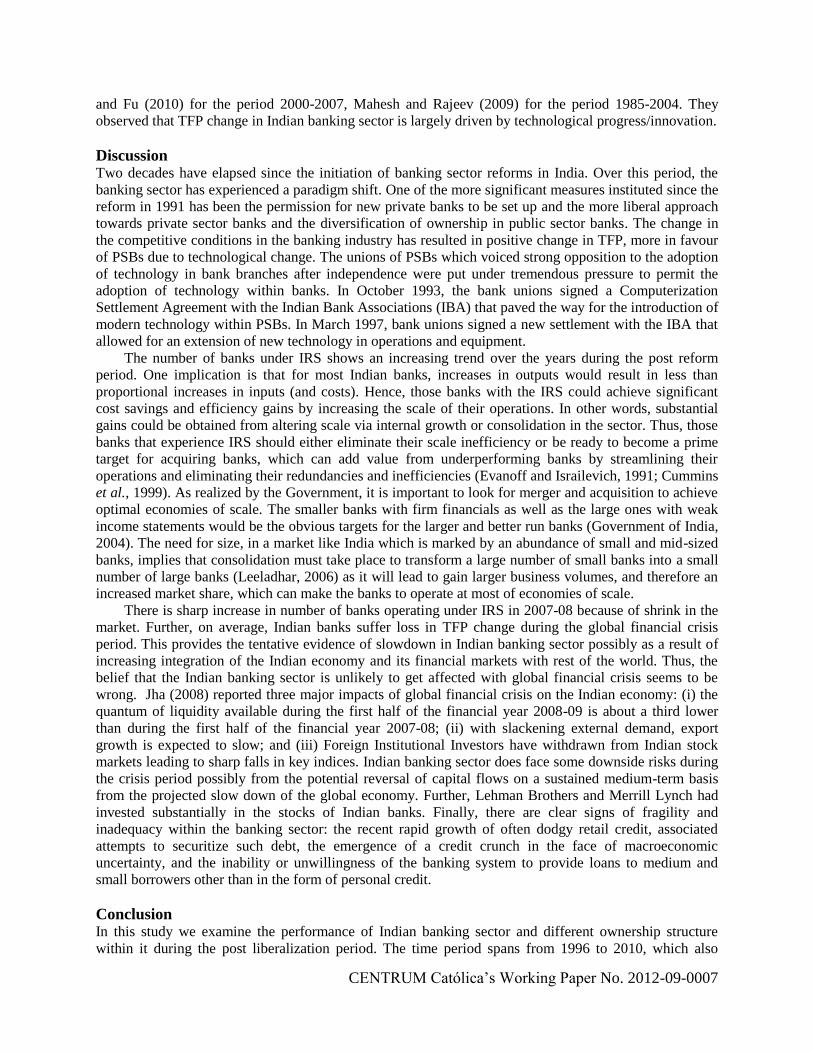
Discussion Two decades have elapsed since the initiation of banking sector reforms in India. Over this period, the

banking sector has experienced a paradigm shift. One of the more significant measures instituted since the

reform in 1991 has been the permission for new private banks to be set up and the more liberal approach

towards private sector banks and the diversification of ownership in public sector banks. The change in

the competitive conditions in the banking industry has resulted in positive change in TFP, more in favour

of PSBs due to technological change. The unions of PSBs which voiced strong opposition to the adoption

of technology in bank branches after independence were put under tremendous pressure to permit the

adoption of technology within banks. In October 1993, the bank unions signed a Computerization

Settlement Agreement with the Indian Bank Associations (IBA) that paved the way for the introduction of

modern technology within PSBs. In March 1997, bank unions signed a new settlement with the IBA that

allowed for an extension of new technology in operations and equipment.

The number of banks under IRS shows an increasing trend over the years during the post reform

period. One implication is that for most Indian banks, increases in outputs would result in less than

proportional increases in inputs (and costs). Hence, those banks with the IRS could achieve significant

cost savings and efficiency gains by increasing the scale of their operations. In other words, substantial

gains could be obtained from altering scale via internal growth or consolidation in the sector. Thus, those

banks that experience IRS should either eliminate their scale inefficiency or be ready to become a prime

target for acquiring banks, which can add value from underperforming banks by streamlining their

operations and eliminating their redundancies and inefficiencies (Evanoff and Israilevich, 1991; Cummins

et al., 1999). As realized by the Government, it is important to look for merger and acquisition to achieve

optimal economies of scale. The smaller banks with firm financials as well as the large ones with weak

income statements would be the obvious targets for the larger and better run banks (Government of India,

2004). The need for size, in a market like India which is marked by an abundance of small and mid-sized

banks, implies that consolidation must take place to transform a large number of small banks into a small

number of large banks (Leeladhar, 2006) as it will lead to gain larger business volumes, and therefore an

increased market share, which can make the banks to operate at most of economies of scale.

There is sharp increase in number of banks operating under IRS in 2007-08 because of shrink in the

market. Further, on average, Indian banks suffer loss in TFP change during the global financial crisis

period. This provides the tentative evidence of slowdown in Indian banking sector possibly as a result of

increasing integration of the Indian economy and its financial markets with rest of the world. Thus, the

belief that the Indian banking sector is unlikely to get affected with global financial crisis seems to be

wrong. Jha (2008) reported three major impacts of global financial crisis on the Indian economy: (i) the

quantum of liquidity available during the first half of the financial year 2008-09 is about a third lower

than during the first half of the financial year 2007-08; (ii) with slackening external demand, export

growth is expected to slow; and (iii) Foreign Institutional Investors have withdrawn from Indian stock

markets leading to sharp falls in key indices. Indian banking sector does face some downside risks during

the crisis period possibly from the potential reversal of capital flows on a sustained medium-term basis

from the projected slow down of the global economy. Further, Lehman Brothers and Merrill Lynch had

invested substantially in the stocks of Indian banks. Finally, there are clear signs of fragility and

inadequacy within the banking sector: the recent rapid growth of often dodgy retail credit, associated

attempts to securitize such debt, the emergence of a credit crunch in the face of macroeconomic

uncertainty, and the inability or unwillingness of the banking system to provide loans to medium and

small borrowers other than in the form of personal credit.

Conclusion In this study we examine the performance of Indian banking sector and different ownership structure

within it during the post liberalization period. The time period spans from 1996 to 2010, which also

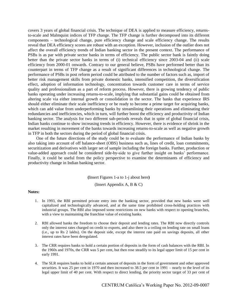
CENTRUM Católica‟s Working Paper No. 2012-09-0007

covers 3 years of global financial crisis. The technique of DEA is applied to measure efficiency, returns-

to-scale and Malmquist indices of TFP change. The TFP change is further decomposed into its different

components – technological change, pure efficiency change and scale efficiency change. The results

reveal that DEA efficiency scores are robust with an exception. However, inclusion of the outlier does not

affect the overall efficiency trends of Indian banking sector in the present context. The performance of

PSBs is as par with private sector banks in terms of efficiency. The public sector bank is faintly doing

better than the private sector banks in terms of (i) technical efficiency since 2003-04 and (ii) scale

efficiency from 2000-01 onwards. Contrary to our general believe, PSBs have performed better than its

counterpart in terms of TFP change as a result of significant differences in technological change. The

performance of PSBs in post reform period could be attributed to the number of factors such as, import of

better risk management skills from private domestic banks, intensified competition, the diversification

effect, adoption of information technology, concentration towards customer care in terms of service

quality and professionalism as a part of reform process. However, there is growing tendency of public

banks operating under increasing returns-to-scale, implying that substantial gains could be obtained from

altering scale via either internal growth or consolidation in the sector. The banks that experience IRS

should either eliminate their scale inefficiency or be ready to become a prime target for acquiring banks,

which can add value from underperforming banks by streamlining their operations and eliminating their

redundancies and inefficiencies, which in turn, will further boost the efficiency and productivity of Indian

banking sector. The analysis for two different sub-periods reveals that in spite of global financial crisis,

Indian banks continue to show increasing trends in efficiency. However, there is evidence of shrink in the

market resulting in movement of the banks towards increasing returns-to-scale as well as negative growth

in TFP in both the sectors during the period of global financial crisis.

One of the future directions of the study could be to evaluate the performance of Indian banks by

also taking into account of off balance-sheet (OBS) business such as, lines of credit, loan commitments,

securitization and derivatives with larger set of sample including the foreign banks. Further, production or

value-added approach could be considered side-by-side to give further insight on banks‟ performance.

Finally, it could be useful from the policy perspective to examine the determinants of efficiency and

productivity change in Indian banking sector.

(Insert Figures 1-a to 1-j about here)

(Insert Appendix A, B & C)

Notes:

1. In 1993, the RBI permitted private entry into the banking sector, provided that new banks were well

capitalized and technologically advanced, and at the same time prohibited cross-holding practices with

industrial groups. The RBI also imposed some restrictions on new banks with respect to opening branches,

with a view to maintaining the franchise value of existing banks.

2. RBI allowed banks the freedom to choose their deposit and lending rates. The RBI now directly controls

only the interest rates charged on credit to exports, and also there is a ceiling on lending rate on small loans

(i.e., up to Rs 2 lakhs). On the deposit side, except the interest rate paid on savings deposits, all other

interest rates have been deregulated.

3. The CRR requires banks to hold a certain portion of deposits in the form of cash balances with the RBI. In

the 1960s and 1970s, the CRR was 5 per cent, but then rose steadily to its legal upper limit of 15 per cent in

early 1991.

4. The SLR requires banks to hold a certain amount of deposits in the form of government and other approved

securities. It was 25 per cent in 1970 and then increased to 38.5 per cent in 1991 – nearly to the level of its

legal upper limit of 40 per cent. With respect to direct lending, the priority sector target of 33 per cent of

CENTRUM Católica‟s Working Paper No. 2012-09-0007

total advances was introduced in 1974, and the ratio was gradually raised to 40 per cent in 1985. There

were sub-targets for agriculture, small farmers, and disadvantaged sections.

5. In 1992, the RBI issued guidelines for income recognition, asset classification and provisioning, and also

adopted the Basle Accord capital adequacy standards. The government also established the Board of

Financial Supervision in the RBI and recapitalized public-sector banks in order to give banks sufficient

financial strength and to enable them to gain access to capital markets.

6. The RBI measures to meet the above objectives came in several policy packages including both

conventional as well as unconventional measures starting mid-September 2008. On the conventional side,

RBI reduced the policy interest rates aggressively and rapidly, reduced the quantum of bank reserves

impounded by the central bank and expanded and liberalized the refinance facilities for export credit.

Measures aimed at managing FOREX liquidity included an upward adjustment of the interest rate ceiling

on the foreign currency deposits by non-resident Indians, substantially relaxing the external commercial

borrowings (ECB) regime for corporates, and allowing non-banking financial companies and housing

finance companies access to foreign borrowing. The important among the many unconventional measures

taken by the RBI are a rupee-dollar swap facility for Indian banks to give them comfort in managing their

short-term foreign funding requirements, an exclusive refinance window as also a special purpose vehicle

for supporting non-banking financial companies, and expanding the lendable resources available to apex

finance institutions for refinancing credit extended to small industries, housing and exports.

7. See Sealey and Lindley, 1977 for a detailed discussion.

8. The justification on choice of intermediary approach in the present case can be viewed in Kumar and

Charles (2011).

9. An increase in the number of outputs or inputs leads to an increase in efficiency scores. In small samples

with many variables almost all units may be on the frontier.

10. The production approach focuses on the bank‟s operating costs, that is, the cost of labour (employees) and

physical capital (plant and equipment). The intermediary approach considers a financial firm‟s production

process to be one of the financial intermediaries (the borrowing of funds and subsequent lending to these

funds). Thus, the focus in the intermediary approach is on the total costs, including both interest and

operating expenses.

Reference

Afrait, S.N. (1972), “Efficiency estimation of production functions”, International Economic Review, Vol. 13, No. 3,

pp. 568-98.

Ahluwalia, I. and Shanker, Q.F.R. (1985). Low productivity and high cost - the managerial challenge, Tata

McGraw-Hill, New Delhi, 56-61.

Aigner, D., Lovell, C.A.K. and Schmidt, P. (1977), “Formulation and estimation of stochastic production function

models”. Journal of Econometrics, Vol. 6 No. 1, pp. 21-37.

Alam, S.I.M. (2001), “A non-parametric approach for assessing productivity dynamics of large U.S. Banks”,

Journal of Money, Credit and Banking, Vol. 33 No. 1, pp. 121-39.

Ataullah, A. and Le, H. (2006), “Economic reforms and bank efficiency in developing countries: the case of Indian

banking industry”, Applied Financial Economics, Vol. 16 No. 9, pp. 653-63.

Avkiran, N.K (1999), Productivity Analysis in the services sector with Data Envelopment Analysis (1st ed.), Camira,

Queensland.

Avkiran, N. K. (2000), “Rising productivity of Australian trading banks under deregulation 1986-1995”, Journal of

Economics and Finance, Vol. 24 No. 2, pp. 122-40.

Banker R.D., Charnes, A. and Cooper, W.W. (1984), “Some models for estimating technical and scale inefficiencies

in data envelopment analysis”, Management Science, Vol. 30 No. 9, pp. 1078-92.

Berg, S. A., Forsund, F. and Jansen, E. S. (1992), “Malmquist indices of productivity growth during the deregulation

of Norwegian banking, 1980-1989”, Scandinavian Journal of Economics, Vol. 94 No. 0, pp. 211-28.

CENTRUM Católica‟s Working Paper No. 2012-09-0007

Berger, A. and Humphrey, D. (1997), “Efficiency of financial institutions: international survey and directions for

future research”, European Journal of Operational Research, Vol. 98 No. 2, pp. 175-212.

Berger, A.N., Demsetz, R.S. and Strahan, P.E. (1999), “The consolidation of the financial services industry: causes,

consequences, and implications for the future”, Journal of Banking and Finance, Vol. 23 No. 2-4, pp. 135-

94.

Bhattacharya, A., Lovell, C.A.K. and Sahay, P. (1997), “The impact of liberalization on the productive efficiency of

Indian commercial banks”, European Journal of Operational Research, Vol. 98 No. 2, pp. 332-45.

Bhide, M.G., Prasad, A. and Ghosh, S. (2001), “Banking sector reforms: a critical overview”, Economic and

Political Weekly, Vol. 36 February–March, pp. 399-408.

Bonesronning, H. and Rattso, J. (1994), “Efficiency variation among the Norwegian high schools: consequences of

equalization policy”, Economics of Education Review, Vol.13 No. 4, pp. 289-304.

Brissimis, S.N., Delis, M.D. and Papanikolaou, N.I. (2008), “Exploring the nexus between banking sector reform

and performance: evidence from newly acceded EU countries. Journal of Banking and Finance, Vol. 32

No. 12, pp. 2674–2683.

Burki, A.A. and Niazi, G.S.K. (2010), “Impact of financial reforms on efficiency of state-owned, private and foreign

banks in Pakistan”, Applied Economics, Vol. 42 No. 24, pp. 3147-60.

Canhoto. A. and Dermine, J. (2003), “A note on banking efficiency in Portugal, new vs. old Banks”, Journal of

Banking and Finance, Vol. 27 No. 11, pp. 2087-98.

Casu, B. (2002), “A comparative study of the cost efficiency of Italian bank conglomerates”, Managerial Finance,

Vol. 28 No. 2, pp. 3-23.

Casu, B. and Molyneux, P. (2003), “A comparative study of efficiency in european banking”, Applied Economics,

Vol. 35 No. 17, pp. 1865-76.

Charles, V., Kumar, M., Zegarra, L.F. and Avolio, B. (2011), “Benchmarking Peruvian banks using data

envelopment analysis”, Journal of Centrum Cathedra, Vol. 4 No. 2, pp. 147-64.

Charnes, A., Cooper, W.W. and Rhodes, E. (1978), “Measuring the efficiency of decision making units”, European

Journal of Operational Research, Vol. 2 No. 6, pp. 429-44.

Coelli, T., Rao, D.S.P. and Battese, G.E. (1998), An Introduction to Efficiency Analysis, Kluwer Academic

Publishers, London.

Cummins, J.D., Tennyson, S. and Weiss, M.A. (1999), “Consolidation and efficiency in the US life insurance

industry”, Journal of Banking and Finance, Vol. 23 No. 2-4, pp. 325-57.

Das, A. (1997). “Measurement of productive efficiency and its decomposition in Indian banking firms”, Asian

Economic Review, Vol. 39 No. 3, pp. 422-39.

Debasish, S.S. (2006), “Efficiency performance in Indian banking: use of data envelopment analysis”, Global

Business Review, Vol. 7 No. 2, pp. 325-33.

Evanoff, D.D. and Israilevich, P.R. (1991), “Productive efficiency in banking”, Economic Perspectives, Vol. 15 No.

4, pp. 11-34.

Färe, R. (1988). Fundamentals of Production Theory, Springer-Verlag, Berlin.

Färe, R., Grosskopf, S., Norris, M. and Zhang, Z. (1994), “Productivity growth, technical progress, and efficiency

change in industrial countries”, American Economic Review, Vol. 84 No.1, pp. 66-83.

Farrell, M.J. (1957). “The measurement of productive efficiency”, Journal of the Royal Statistical Society, Vol. 120

No. 3, pp. 253-81.

Fethi, M.D. and Pasiouras, F. (2010), “Assessing bank efficiency and performance with operational research and

artificial intelligent techniques: a survey”, European Journal of Operational Research, Vol. 204 No. 2, pp.

189-98.

Fethi, M.D., Shaban, M. and Weyman-Jones, T. (2011), “Liberalisation, privatization and the productivity of

Egyptian banks: a non-parametric approach”, The Service Industries Journal, Vol. 31 No. 7, pp. 1143-63.

Fu, X. and Heffernan, S. (2009), “The effects of reform on China‟s bank structure and performance”, Journal of

Banking and Finance, Vol. 33 No. 1, pp. 39-52.

Galagedera, D.U.A. and Edirisuriya, P. (2005), “Performance of Indian commercial banks (1995-2002)”, South

Asian Journal of Management, Vol. 12 No. 4, pp. 52-74.

Ghosh, S. (2009), “Charter value and risk-taking: evidence from Indian banks”, Journal of the Asia Pacific

Economy, Vol. 14 No. 3, pp. 270-86.

Gilbert, R. Al. and Wilson, P. W. (1998), “Effect of deregulation on the productivity of Korean banks”, Journal of

Economics and Business, Vol. 50 No. 2, pp. 133-55.

Government of India. (2004). Consolidation in Indian banking System. Working Group Report, Indian Bank

Association (IBA): Publication Department, Stadium House, New Delhi.

CENTRUM Católica‟s Working Paper No. 2012-09-0007

Government of India (2010). Branch banking statistics, Annual Report 2009, Reserve Bank of India, Vol. 4.

Grosskopf, S. (1986), “The role of the reference technology in measuring productive efficiency”, Economic Journal,

Vol. 96 June, pp. 499-513.

Gupta, O.K., Doshit, Y. and Chinubhai, A. (2008), “Dynamics of productive efficiency of Indian banks”,

International Journal of Operations Research, Vol. 5 No. 2, pp. 78-90.

Hasan, I. and Marton, K. (2003), “Development and efficiency of the banking sector in a transitional economy:

Hungarian experience”, Journal of Banking and Finance, Vol. 27 No. 7, pp. 2249-71.

Havrylchyk, O. (2006), “Efficiency of the Polish banking industry: Foreign versus domestic banks”, Journal of

Banking and Finance, Vol. 30 No. 7, pp. 1975-96.

Heffernan, S. A. and Fu, X. (2010), “Bank productivity changes in two Asian giants”, Proceedings of the 8th

INFINITI Conference on International Finance, Dublin.

Hsiao, H.-C., Chang, H., Cianci, A.M. and Huang, L.-H. (2010), “First financial restructuring and operating

efficiency: evidence from Taiwanese commercial banks”, Journal of Banking and Finance, Vol. 34 No. 7,

pp. 1461-71.

Humphrey, D.B. (1985), “Costs and scale economies in bank intermediation”, in Aspinwall, R.C. and Eisenbeis,

R.A. (Eds.), Handbook for Banking Strategy, John Wiley and Sons, New York, NY, pp. 745-83.

Isik, I. and Hassan, M.K. (2002a), “Technical, scale and allocative efficiencies of Turkish banking Industry”,

Journal of Banking and Finance, Vol. 26 No. 4, pp. 719-66.

Isik, I. and Hassan, M.K. (2002b), “Cost and profit efficiency of the Turkish banking industry: an empirical

investigation”, The Financial Review, Vol. 37 No. 2, pp. 257-80.

Isik, I. and Hassan, M.K. (2003), “Financial deregulation and total factor productivity change: an empirical study of

Turkish commercial banks”, Journal of Banking and Finance, Vol. 27 No. 8, pp. 1455-85.

Jha, R. (2008), India: Confronting the Global Financial Crisis, East Asia Forum, available at:

http://www.eastasiaforum.org/2008/11/15/india-confronting-the-global-financial-crisis (accessed 17th

August 2012).

Kao, C. and Liu, S. (2004), “Predicting bank performance with financial forecasts: a case of Taiwan commercial

banks”, Journal of Banking & Finance, Vol. 28 No. 10, pp. 2353-68.

Kumar, M. and Basu, P. (2004), “Decomposition of productivity growth using data envelopment analysis: a case

study of Indian industrial machinery”, in Nagarjuna B. (Ed.), Economic Reforms and Perspectives, Serial

Publication, New Delhi, pp. 347-70.

Kumar, M. and Charles, V. (2011), “Benchmarking Indian banks using DEA in post-liberalization period:

progressive time-weighted mean approach”, The Service Industries Journal, Vol. 31 No. 14, pp. 2455-85.

Kumar, M. and Charles, V. (2009), “Productivity growth as the indicator of shareholders‟ wealth maximization: an

empirical investigation”, Journal of Centrum Cathedra, Vol. 2 No. 1, pp. 73-85.

Kumar, L., Malathy, D. and Ganesh, L.S. (2010), “Productivity growth and efficiency change in Indian banking:

Technology effect vs. catch-up effect”, Journal of Advances in Management Research, Vol. 7 No. 2, pp.

194-218.

Kumbhakar, S.C. and Sarkar, S. (2005). “Deregulation, ownership and efficiency change in Indian banking: an

application of stochastic frontier analysis”, in Ghosh R. and Neogi C. (Eds.), Theory and Application of

Productivity and Efficiency: Econometric and DEA Approach. Macmillan, India.

Leeladhar, V. (2006), Consolidation: boosting the banking sector, The Financial Express, available at:

http://www.financialexpress.com/news/consolidation-boosting-the-banking-sector/177149/3 (accessed 17th

August 2012)

Leightner, J.E. and Lovell, C.A.K. (1998). “The impact of financial liberalization on the performance of Thai

banks”, Journal of Economics and Business, Vol. 50 No. 2, pp. 115-31.

Mahesh, H.P. and Rajeev, M. (2009). “Producing financial services: an efficiency analysis of Indian commercial

banks”, Journal of Service Research, Vol. 8 No. 2, pp. 7-29.

Mohan, R. (2008). Global Financial Crisis and Key Risks: Impact on India and Asia, Remarks prepared for IMF-

FSF High-level Meeting on Recent Financial Turmoil and Policy Responses, Washington D.C.

Mostafa, M. (2010), “Does efficiency matter? Examining the efficiency-profitability link in the US specialty

retailers and food consumer stores”, International Journal of Productivity and Performance Management,

Vol. 59 No. 3, pp. 255-73.

Mukherjee, K., Ray, S.C. and Miller, S.M. (2001), “Productivity growth in large US commercial banks: the initial

post-deregulation experience”, Journal of Banking and Finance, Vol. 25 No. 5, pp. 913-39.

Nunamaker, T.R. (1985), “Using data envelopment analysis to measure the efficiency of non-profit organizations”,

Managerial and Decision Making, Vol. 6 No. 1, pp. 50-58.

CENTRUM Católica‟s Working Paper No. 2012-09-0007

Prasad, A. and Ghosh, S. (2007), “Competition in Indian banking: an empirical evaluation”, South Asia Economics

Journal, Vol. 8 No. 2, pp. 265-84.

Prasad, A. and Reddy, C.P. (2009), “Global financial crisis and its impact on India”, Journal of Social Sciences, Vol.

21 No. 1, pp. 1-5.

Ram Mohan, T.T. (2005), Privatization in India: challenging economic orthodoxy, Taylor & Francis Group, New

York, NY.

Ram Mohan, T.T. and Ray, S.C. (2003), “Productivity and efficiency at public and private sector banks in India”,

IIMA Working Paper Series WP2003-06-0, Indian Institute of Management Publication Department,

Ahmedabad.

Ram Mohan, T.T. and Ray, S.C. (2004), “Productivity growth and efficiency in Indian banking: a comparison of

public, private, and foreign banks”, Economics Working Paper 2004-27, Department of Economics,

University of Connecticut, Storrs, CT.

Raab, R. and Lichty, R. (2002), “Identifying sub-areas that comprise a greater metropolitan area: the criterion of

country relative efficiency”, Journal of Regional Science, Vol. 42 No. 3, pp. 579-94.

Ray, S.C. and Desli, E. (1997), “Productivity growth, technical progress, and efficiency changes in industrialized

countries: comment”, American Economic Review, Vol. 87 No. 5, pp. 1033-39.

Reddy, Y.V. (2006), “Reforming India‟s Financial Sector: Changing Dimensions and Emerging Issues”, Address

Delivered at the International Center for Monetary and Banking Studies, Geneva.

Saha, A. and Ravisankar, T.S. (2000), “Rating of Indian commercial banks: a DEA approach”, European Journal of

Operational Research, Vol. 124 No. 1, pp. 187- 203.

Sahoo, B. K., Sengupta, J. K. and Mandal, A. (2007), “Productive performance evaluation of the banking sector in

India using data envelopment analysis”, International Journal of Operations Research, Vol. 4 No. 2, pp.

63-79.

Sathye, M. (2003), “Efficiency of banks in a developing economy: the case of India”, European Journal of

Operational Research, Vol. 148 No. 3, pp. 662-71.

Sealey, C.W. Jr. and Lindley, J.T. (1977), “Inputs, outputs, and a theory of production and cost at depository

financial institutions”, Journal of Finance, Vol. 32 No. 4, pp. 1251-66.

Shephard, R.W. (1970), Theory of Cost and Production Function, Princeton University Press, Princeton, NJ.

Sinha, R.P. (2008). “Ownership and efficiency: a non-radial bilateral performance comparison of Indian commercial

banks”, The Icfai University Journal of Managerial Economics, Vol. 6 No. 4, pp. 67-81.

Smith, P. (1997), “Model misspecification in data envelopment analysis”, Annals of Operations Research, Vol. 73

No. 1, pp. 233-52.

Sturm, J-E. and Williams, B. (2004), “Foreign bank entry, deregulation and bank efficiency: lessons from the

Australian experience”, Journal of Banking and Finance, Vol. 28 No. 7, pp. 1775-99.

Subbarao, D. (2009), “Impact of the global financial crisis on India collateral damage and response” Speech

delivered at the Symposium on The Global Economic Crisis and Challenges for the Asian economy in a

Changing World, organized by the Institute for International Monetary Affairs, Tokyo.

Udhayakumar, A., Charles, V. and Kumar, M. (2011), “Stochastic simulation based genetic algorithm for chance

constrained data envelopment analysis problems”, Omega, Vol. 39 No. 4, pp. 387-97.

Yeh, Q.J. (1996), “The application of data envelopment analysis in conjunction with financial ratios for bank

performance evaluation”, Journal of the Operational Research Society, Vol. 47 No. 8, pp. 980-88.

Yildirim, H.S. and Philippatos, G.C. (2007), “Efficiency of banks: recent evidence from the transition economies of

Europe 1993-2000”, European Journal of Finance, Vol. 13 No. 2, pp. 123-43.

Zaim, O. (1995), “The Effect of financial liberalization on the efficiency of Turkish commercial banks”, Applied

Financial Economics, Vol. 5 No. 4, pp. 275-64.

Zhao, T., Casu, B. and Ferrari, A. (2008). “Deregulation and productivity growth: a study of the Indian commercial

banking industry”, International Journal of Business Performance Management, Vol. 10 No. 4, pp. 318-43.

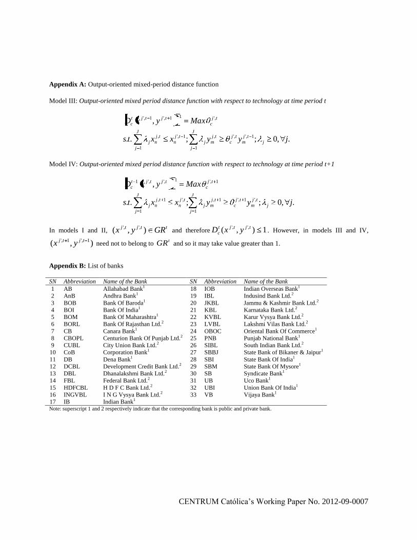
CENTRUM Católica‟s Working Paper No. 2012-09-0007

Appendix A: Output-oriented mixed-period distance function

Model III: Output-oriented mixed period distance function with respect to technology at time period t

.,0;;..

,

1

1,',',

1

1,',

,'11,'1,'

jyyxxts

MaxyxD

j

J

j

tj

m

tj

c

tj

mj

J

j

tj

n

tj

nj

tj

c

tjtjt

c

Model IV: Output-oriented mixed period distance function with respect to technology at time period t+1

.,0;;..

,

1

,'1,'1,

1

,'1,

1,'1,','1

jyyxxts

MaxyxD

j

J

j

tj

m

tj

c

tj

mj

J

j

tj

n

tj

nj

tj

c

tjtjt

c

In models I and II, ttjtj GRyx ),( ,','

and therefore 1),( ,',' tjtjt

c yxD . However, in models III and IV,

),( 1,'1,' tjtj yx need not to belong to tGR and so it may take value greater than 1.

Appendix B: List of banks

SN Abbreviation Name of the Bank SN Abbreviation Name of the Bank

1 AB Allahabad Bank1 18 IOB Indian Overseas Bank1

2 AnB Andhra Bank1 19 IBL Indusind Bank Ltd.2

3 BOB Bank Of Baroda1 20 JKBL Jammu & Kashmir Bank Ltd.2

4 BOI Bank Of India1 21 KBL Karnataka Bank Ltd.2

5 BOM Bank Of Maharashtra1 22 KVBL Karur Vysya Bank Ltd.2

6 BORL Bank Of Rajasthan Ltd.2 23 LVBL Lakshmi Vilas Bank Ltd.2

7 CB Canara Bank1 24 OBOC Oriental Bank Of Commerce1

8 CBOPL Centurion Bank Of Punjab Ltd.2 25 PNB Punjab National Bank1

9 CUBL City Union Bank Ltd.2 26 SIBL South Indian Bank Ltd.2

10 CoB Corporation Bank1 27 SBBJ State Bank of Bikaner & Jaipur1

11 DB Dena Bank1 28 SBI State Bank Of India1

12 DCBL Development Credit Bank Ltd.2 29 SBM State Bank Of Mysore1

13 DBL Dhanalakshmi Bank Ltd.2 30 SB Syndicate Bank1

14 FBL Federal Bank Ltd.2 31 UB Uco Bank1

15 HDFCBL H D F C Bank Ltd.2 32 UBI Union Bank Of India1

16 INGVBL I N G Vysya Bank Ltd.2 33 VB Vijaya Bank1

17 IB Indian Bank1 Note: superscript 1 and 2 respectively indicate that the corresponding bank is public and private bank.

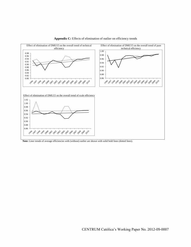
CENTRUM Católica‟s Working Paper No. 2012-09-0007

Appendix C: Effects of elimination of outlier on efficiency trends

Effect of elimination of DMU15 on the overall trend of technical

efficiency

Effect of elimination of DMU15 on the overall trend of pure

technical efficiency

Effect of elimination of DMU15 on the overall trend of scale efficiency

Note: Liner trends of average efficiencies with (without) outlier are shown with solid bold lines (dotted lines).

0.80

0.82

0.84

0.86

0.88

0.90

0.92

0.94

0.96

0.98

0.86

0.88

0.90

0.92

0.94

0.96

0.98

1.00

0.86

0.88

0.90

0.92

0.94

0.96

0.98

1.00

1.02

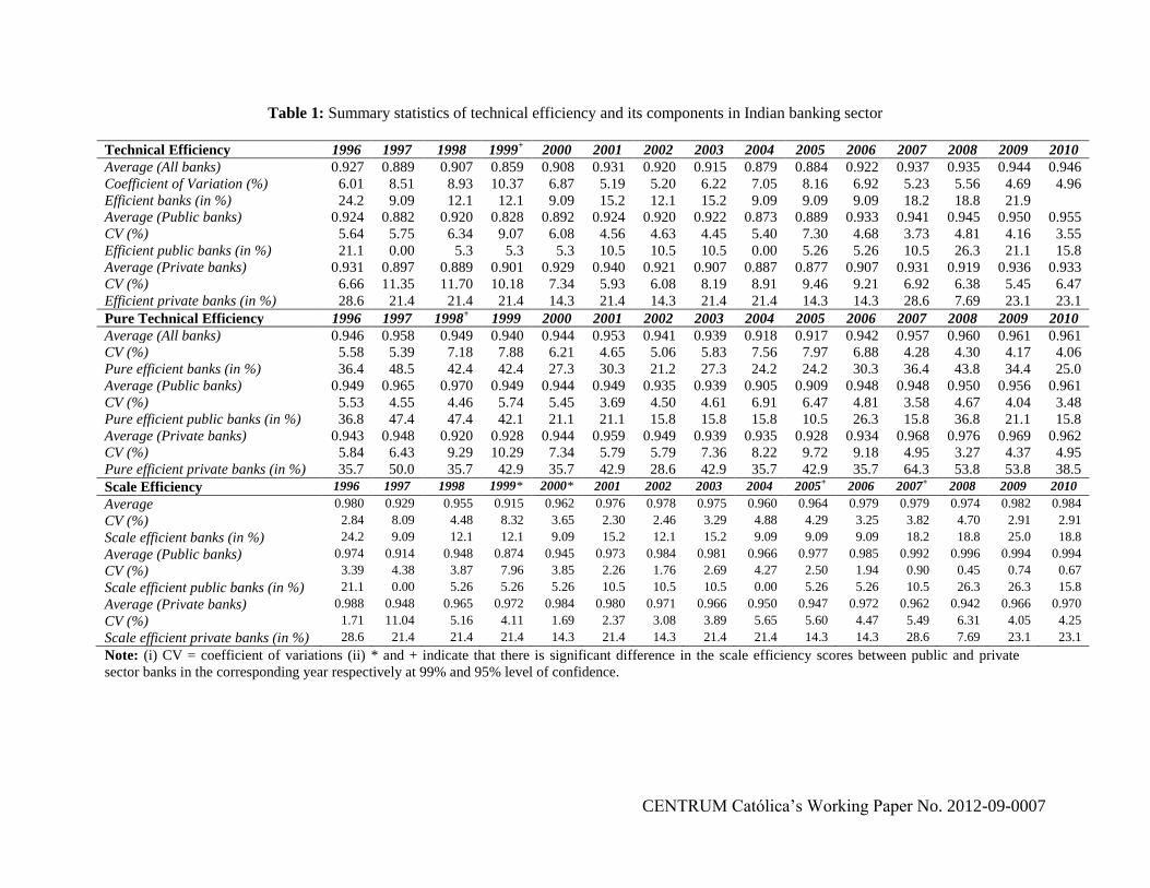
CENTRUM Católica‟s Working Paper No. 2012-09-0007

Table 1: Summary statistics of technical efficiency and its components in Indian banking sector

Technical Efficiency 1996 1997 1998 1999

+ 2000 2001 2002 2003 2004 2005 2006 2007 2008 2009 2010

Average (All banks) 0.927 0.889 0.907 0.859 0.908 0.931 0.920 0.915 0.879 0.884 0.922 0.937 0.935 0.944 0.946

Coefficient of Variation (%) 6.01 8.51 8.93 10.37 6.87 5.19 5.20 6.22 7.05 8.16 6.92 5.23 5.56 4.69 4.96

Efficient banks (in %) 24.2 9.09 12.1 12.1 9.09 15.2 12.1 15.2 9.09 9.09 9.09 18.2 18.8 21.9

Average (Public banks) 0.924 0.882 0.920 0.828 0.892 0.924 0.920 0.922 0.873 0.889 0.933 0.941 0.945 0.950 0.955

CV (%) 5.64 5.75 6.34 9.07 6.08 4.56 4.63 4.45 5.40 7.30 4.68 3.73 4.81 4.16 3.55

Efficient public banks (in %) 21.1 0.00 5.3 5.3 5.3 10.5 10.5 10.5 0.00 5.26 5.26 10.5 26.3 21.1 15.8

Average (Private banks) 0.931 0.897 0.889 0.901 0.929 0.940 0.921 0.907 0.887 0.877 0.907 0.931 0.919 0.936 0.933

CV (%) 6.66 11.35 11.70 10.18 7.34 5.93 6.08 8.19 8.91 9.46 9.21 6.92 6.38 5.45 6.47

Efficient private banks (in %) 28.6 21.4 21.4 21.4 14.3 21.4 14.3 21.4 21.4 14.3 14.3 28.6 7.69 23.1 23.1

Pure Technical Efficiency 1996 1997 1998+ 1999 2000 2001 2002 2003 2004 2005 2006 2007 2008 2009 2010

Average (All banks) 0.946 0.958 0.949 0.940 0.944 0.953 0.941 0.939 0.918 0.917 0.942 0.957 0.960 0.961 0.961

CV (%) 5.58 5.39 7.18 7.88 6.21 4.65 5.06 5.83 7.56 7.97 6.88 4.28 4.30 4.17 4.06

Pure efficient banks (in %) 36.4 48.5 42.4 42.4 27.3 30.3 21.2 27.3 24.2 24.2 30.3 36.4 43.8 34.4 25.0

Average (Public banks) 0.949 0.965 0.970 0.949 0.944 0.949 0.935 0.939 0.905 0.909 0.948 0.948 0.950 0.956 0.961

CV (%) 5.53 4.55 4.46 5.74 5.45 3.69 4.50 4.61 6.91 6.47 4.81 3.58 4.67 4.04 3.48

Pure efficient public banks (in %) 36.8 47.4 47.4 42.1 21.1 21.1 15.8 15.8 15.8 10.5 26.3 15.8 36.8 21.1 15.8

Average (Private banks) 0.943 0.948 0.920 0.928 0.944 0.959 0.949 0.939 0.935 0.928 0.934 0.968 0.976 0.969 0.962

CV (%) 5.84 6.43 9.29 10.29 7.34 5.79 5.79 7.36 8.22 9.72 9.18 4.95 3.27 4.37 4.95

Pure efficient private banks (in %) 35.7 50.0 35.7 42.9 35.7 42.9 28.6 42.9 35.7 42.9 35.7 64.3 53.8 53.8 38.5

Scale Efficiency 1996 1997 1998 1999* 2000* 2001 2002 2003 2004 2005+ 2006 2007+ 2008 2009 2010

Average 0.980 0.929 0.955 0.915 0.962 0.976 0.978 0.975 0.960 0.964 0.979 0.979 0.974 0.982 0.984

CV (%) 2.84 8.09 4.48 8.32 3.65 2.30 2.46 3.29 4.88 4.29 3.25 3.82 4.70 2.91 2.91

Scale efficient banks (in %) 24.2 9.09 12.1 12.1 9.09 15.2 12.1 15.2 9.09 9.09 9.09 18.2 18.8 25.0 18.8

Average (Public banks) 0.974 0.914 0.948 0.874 0.945 0.973 0.984 0.981 0.966 0.977 0.985 0.992 0.996 0.994 0.994

CV (%) 3.39 4.38 3.87 7.96 3.85 2.26 1.76 2.69 4.27 2.50 1.94 0.90 0.45 0.74 0.67

Scale efficient public banks (in %) 21.1 0.00 5.26 5.26 5.26 10.5 10.5 10.5 0.00 5.26 5.26 10.5 26.3 26.3 15.8

Average (Private banks) 0.988 0.948 0.965 0.972 0.984 0.980 0.971 0.966 0.950 0.947 0.972 0.962 0.942 0.966 0.970

CV (%) 1.71 11.04 5.16 4.11 1.69 2.37 3.08 3.89 5.65 5.60 4.47 5.49 6.31 4.05 4.25

Scale efficient private banks (in %) 28.6 21.4 21.4 21.4 14.3 21.4 14.3 21.4 21.4 14.3 14.3 28.6 7.69 23.1 23.1

Note: (i) CV = coefficient of variations (ii) * and + indicate that there is significant difference in the scale efficiency scores between public and private

sector banks in the corresponding year respectively at 99% and 95% level of confidence.

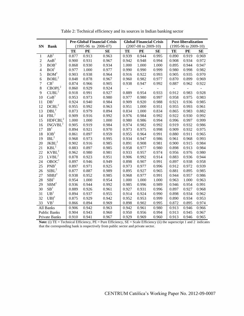
CENTRUM Católica‟s Working Paper No. 2012-09-0007

Table 2: Technical efficiency and its sources in Indian banking sector

SN Bank

Pre-Global Financial Crisis

(1995-96 to 2006-07) Global Financial Crisis

(2007-08 to 2009-10) Post-liberalization

(1995-96 to 2009-10)

TE PE SE TE PE SE TE PE SE

1 AB1 0.877 0.913 0.963 0.939 0.944 0.995 0.890 0.919 0.969

2 AnB1 0.900 0.931 0.967 0.942 0.948 0.994 0.908 0.934 0.972

3 BOB1 0.868 0.930 0.934 1.000 1.000 1.000 0.895 0.944 0.947

4 BOI1 0.977 1.000 0.977 0.990 0.990 0.999 0.980 0.998 0.982

5 BOM1 0.903 0.938 0.964 0.916 0.922 0.993 0.905 0.935 0.970

6 BORL2 0.848 0.878 0.967 0.960 0.982 0.977 0.870 0.899 0.969

7 CB1 0.874 0.966 0.905 0.938 0.947 0.992 0.887 0.962 0.922

8 CBOPL2 0.860 0.929 0.924 - - - - - -

9 CUBL2 0.918 0.991 0.927 0.889 0.954 0.933 0.912 0.983 0.928

10 CoB1 0.953 0.973 0.980 0.977 0.980 0.997 0.958 0.975 0.983

11 DB1 0.924 0.940 0.984 0.909 0.920 0.988 0.921 0.936 0.985

12 DCBL2 0.955 0.992 0.963 0.951 1.000 0.951 0.955 0.993 0.961

13 DBL2 0.873 0.979 0.894 0.834 1.000 0.834 0.865 0.983 0.882

14 FBL2 0.909 0.916 0.992 0.976 0.984 0.992 0.922 0.930 0.992

15 HDFCBL2 1.000 1.000 1.000 0.980 0.986 0.994 0.996 0.997 0.999

16 INGVBL2 0.905 0.919 0.984 0.974 0.982 0.992 0.919 0.932 0.986

17 IB1 0.894 0.921 0.970 0.973 0.975 0.998 0.909 0.932 0.975

18 IOB1 0.861 0.897 0.959 0.955 0.964 0.991 0.880 0.911 0.965

19 IBL2 0.968 0.973 0.995 0.934 0.947 0.986 0.961 0.968 0.993

20 JKBL2 0.902 0.916 0.985 0.891 0.908 0.981 0.900 0.915 0.984

21 KBL2 0.883 0.897 0.985 0.958 0.977 0.980 0.898 0.913 0.984

22 KVBL2 0.962 0.980 0.981 0.933 0.957 0.974 0.956 0.976 0.980

23 LVBL2 0.878 0.923 0.951 0.906 0.992 0.914 0.883 0.936 0.944

24 OBOC1 0.897 0.946 0.949 0.898 0.907 0.991 0.897 0.938 0.958

25 PNB1 0.897 0.971 0.925 0.973 0.977 0.996 0.912 0.972 0.939

26 SIBL2 0.877 0.887 0.989 0.895 0.927 0.965 0.881 0.895 0.985

27 SBBJ1 0.938 0.952 0.985 0.968 0.977 0.991 0.944 0.957 0.986

28 SBI1 0.954 1.000 0.954 1.000 1.000 1.000 0.963 1.000 0.963

29 SBM1 0.936 0.944 0.992 0.985 0.996 0.989 0.946 0.954 0.991

30 SB1 0.889 0.926 0.961 0.927 0.931 0.996 0.897 0.927 0.968

31 UB1 0.894 0.937 0.955 0.914 0.924 0.990 0.898 0.934 0.962

32 UBI1 0.875 0.929 0.942 0.952 0.953 0.999 0.890 0.934 0.953

33 VB1

0.866 0.894 0.969 0.898 0.902 0.995 0.872 0.895 0.974

All Banks 0.906 0.942 0.963 0.942 0.961 0.980 0.913 0.946 0.966

Public Banks 0.904 0.943 0.960 0.950 0.956 0.994 0.913 0.945 0.967

Private Banks 0.910 0.941 0.967 0.929 0.969 0.960 0.913 0.946 0.965

Note: (i) TE = Technical Efficiency, PE = Pure Efficiency, SE = Scale Efficiency (ii) the superscript 1 and 2 indicates

that the corresponding bank is respectively from public sector and private sector.

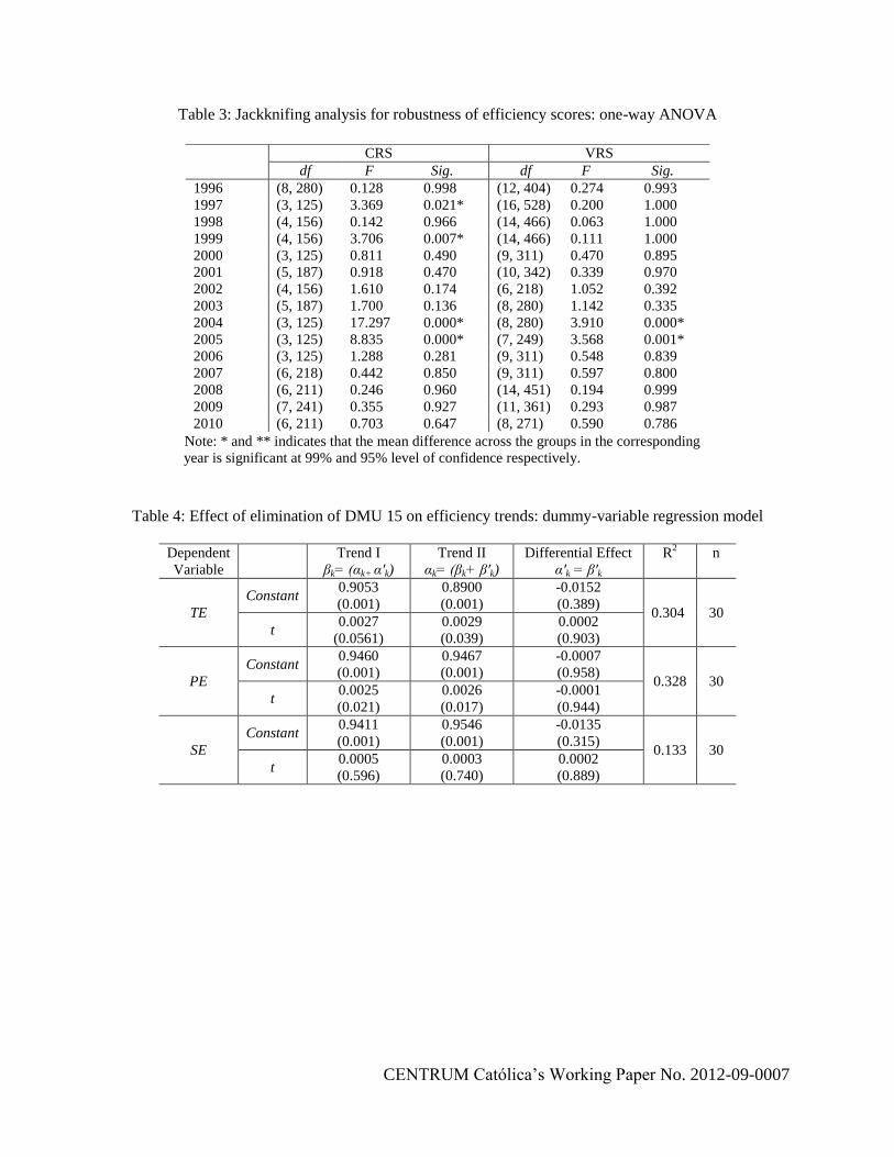
CENTRUM Católica‟s Working Paper No. 2012-09-0007

Table 3: Jackknifing analysis for robustness of efficiency scores: one-way ANOVA

Note: * and ** indicates that the mean difference across the groups in the corresponding

year is significant at 99% and 95% level of confidence respectively.

Table 4: Effect of elimination of DMU 15 on efficiency trends: dummy-variable regression model

Dependent

Variable

Trend I

βk= (αk+ α'k)

Trend II

αk= (βk+ β'k)

Differential Effect

α'k = β'k

R2 n

TE

Constant 0.9053

(0.001)

0.8900

(0.001)

-0.0152

(0.389) 0.304 30

t 0.0027

(0.0561)

0.0029

(0.039)

0.0002

(0.903)

PE

Constant 0.9460

(0.001)

0.9467

(0.001)

-0.0007

(0.958) 0.328 30

t 0.0025

(0.021)

0.0026

(0.017)

-0.0001

(0.944)

SE

Constant 0.9411

(0.001)

0.9546

(0.001)

-0.0135

(0.315) 0.133 30

t 0.0005

(0.596)

0.0003

(0.740)

0.0002

(0.889)

CRS VRS

df F Sig. df F Sig.

1996 (8, 280) 0.128 0.998 (12, 404) 0.274 0.993

1997 (3, 125) 3.369 0.021* (16, 528) 0.200 1.000

1998 (4, 156) 0.142 0.966 (14, 466) 0.063 1.000

1999 (4, 156) 3.706 0.007* (14, 466) 0.111 1.000

2000 (3, 125) 0.811 0.490 (9, 311) 0.470 0.895

2001 (5, 187) 0.918 0.470 (10, 342) 0.339 0.970

2002 (4, 156) 1.610 0.174 (6, 218) 1.052 0.392

2003 (5, 187) 1.700 0.136 (8, 280) 1.142 0.335

2004 (3, 125) 17.297 0.000* (8, 280) 3.910 0.000*

2005 (3, 125) 8.835 0.000* (7, 249) 3.568 0.001*

2006 (3, 125) 1.288 0.281 (9, 311) 0.548 0.839

2007 (6, 218) 0.442 0.850 (9, 311) 0.597 0.800

2008 (6, 211) 0.246 0.960 (14, 451) 0.194 0.999

2009 (7, 241) 0.355 0.927 (11, 361) 0.293 0.987

2010 (6, 211) 0.703 0.647 (8, 271) 0.590 0.786

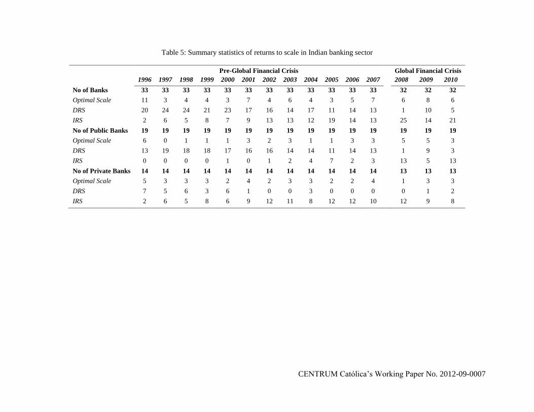
CENTRUM Católica‟s Working Paper No. 2012-09-0007

Table 5: Summary statistics of returns to scale in Indian banking sector

Pre-Global Financial Crisis Global Financial Crisis

1996 1997 1998 1999 2000 2001 2002 2003 2004 2005 2006 2007 2008 2009 2010

No of Banks 33 33 33 33 33 33 33 33 33 33 33 33 32 32 32

Optimal Scale 11 3 4 4 3 7 4 6 4 3 5 7 6 8 6

DRS 20 24 24 21 23 17 16 14 17 11 14 13 1 10 5

IRS 2 6 5 8 7 9 13 13 12 19 14 13 25 14 21

No of Public Banks 19 19 19 19 19 19 19 19 19 19 19 19 19 19 19

Optimal Scale 6 0 1 1 1 3 2 3 1 1 3 3 5 5 3

DRS 13 19 18 18 17 16 16 14 14 11 14 13 1 9 3

IRS 0 0 0 0 1 0 1 2 4 7 2 3 13 5 13

No of Private Banks 14 14 14 14 14 14 14 14 14 14 14 14 13 13 13

Optimal Scale 5 3 3 3 2 4 2 3 3 2 2 4 1 3 3

DRS 7 5 6 3 6 1 0 0 3 0 0 0 0 1 2

IRS 2 6 5 8 6 9 12 11 8 12 12 10 12 9 8

CENTRUM Católica‟s Working Paper No. 2012-09-0007

Table 6: Sources of TFP change in Indian banking sector

SN

Bank

Pre-Global Financial Crisis

(1995-96 to 2006-07)

Global Financial Crisis

(2007-08 to 2009-10)

Post-liberalization

(1995-96 to 2009-10)

TC PEC SEC TFPC TC PEC SEC TFPC TC PEC SEC TFPC

1 AB1 1.69 -0.14 0.02 1.61 0.46 1.68 -0.23 1.93 1.43 0.25 -0.03 1.68

2 AnB1 2.61 0.24 -0.05 2.82 -1.99 0.22 -0.34 -2.08 1.63 0.24 -0.11 1.77

3 BOB1 0.89 -0.36 0.60 1.11 1.32 2.04 0.17 3.54 0.98 0.15 0.51 1.63

4 BOI1 2.48 0.00 0.53 3.01 -0.47 -0.98 -0.03 -1.49 1.85 -0.21 0.41 2.04

5 BOM1 0.52 -0.82 0.01 -0.31 -0.34 -0.65 -0.04 -1.02 0.33 -0.79 0.00 -0.46

6 BORL2 -1.11 0.34 -0.67 -1.43 -7.32 2.83 2.58 -1.91 -2.44 0.88 0.02 -1.53

7 CB1 3.72 -0.64 0.35 3.43 -0.02 0.48 0.18 0.68 2.92 -0.40 0.31 2.84

8 CBOPL2 2.44 0.01 0.00 2.44 - - - - 2.44 0.01 0.00 2.44

9 CUBL2 0.72 0.91 -0.29 1.34 -0.66 -3.64 -1.07 -5.41 0.43 -0.06 -0.45 -0.10

10 CoB1 4.25 0.87 0.00 5.14 -0.58 0.00 0.00 -0.60 3.21 0.68 0.00 3.91

11 DB1 0.59 -0.51 0.04 0.12 -0.32 0.03 -0.47 -0.81 0.39 -0.39 -0.07 -0.08

12 DCBL2 0.15 0.00 -0.63 -0.45 -0.30 0.00 2.27 1.97 0.05 0.00 0.00 0.07

13 DBL2 0.81 1.23 -1.84 0.19 -0.60 0.00 1.33 0.77 0.51 0.97 -1.16 0.32

14 FBL2 -0.49 0.14 0.38 0.01 -0.69 1.05 -0.13 0.20 -0.54 0.34 0.27 0.05

15 HDFCBL2 3.51 0.00 0.00 3.51 -2.86 -1.43 -0.07 -4.31 2.15 -0.31 -0.02 1.84

16 INGVBL2 2.11 1.18 0.45 3.71 -0.44 0.00 0.01 -0.45 1.56 0.93 0.36 2.82

17 IB1 -1.38 0.59 0.41 -0.39 -0.31 -0.41 -0.07 -0.82 -1.15 0.38 0.31 -0.48

18 IOB1 1.63 0.54 0.06 2.20 -1.66 -0.41 0.12 -2.01 0.92 0.34 0.08 1.30

19 IBL2 2.41 -1.23 -0.19 0.98 0.20 4.26 0.26 4.71 1.94 -0.05 -0.10 1.78

20 JKBL2 2.78 -0.01 0.00 2.80 -1.84 -5.42 -0.58 -7.80 1.79 -1.17 -0.12 0.53

21 KBL2 -0.62 0.16 -0.13 -0.57 -2.70 1.68 0.17 -0.91 -1.07 0.48 -0.06 -0.64

22 KVBL2 1.87 0.07 0.12 2.06 -0.15 -1.96 -0.60 -2.73 1.44 -0.36 -0.03 1.04

23 LVBL2 1.60 0.46 -0.63 1.42 0.26 -0.84 0.23 -0.36 1.31 0.18 -0.45 1.04

24 OBOC1 2.87 -0.84 -0.05 2.00 0.11 -0.86 -0.17 -0.92 2.28 -0.85 -0.07 1.38

25 PNB1 2.22 -0.60 0.71 2.34 -0.09 0.33 0.23 0.41 1.73 -0.40 0.60 1.93

26 SIBL2 1.13 0.19 -0.08 1.28 -0.88 0.93 -1.06 -1.00 0.70 0.35 -0.29 0.79

27 SBBJ1 1.18 0.44 -0.01 1.63 0.22 1.58 -0.47 1.28 0.97 0.68 -0.11 1.55

28 SBI1 -0.68 0.00 0.01 -0.67 0.92 0.00 0.00 0.92 -0.34 0.00 0.01 -0.33

29 SBM1 1.58 1.72 -0.01 3.28 -0.18 -0.37 -0.71 -1.29 1.20 1.27 -0.16 2.30

30 SB1 3.97 -0.77 -0.20 3.02 -1.30 2.31 0.20 1.22 2.84 -0.11 -0.12 2.63

31 UB1 3.18 -0.19 0.48 3.45 0.27 0.99 -0.57 0.73 2.56 0.07 0.26 2.87

32 UBI1 3.86 0.87 0.35 5.09 0.69 0.24 -0.03 0.95 3.18 0.73 0.27 4.20

33 VB1 2.22 -0.35 -0.02 1.82 -1.64 0.90 -0.17 -0.91 1.39 -0.09 -0.05 1.23

All Banks 1.66 0.11 -0.01 1.76 -0.72 0.14 0.03 -0.55 1.16 0.11 0.00 1.27

Public Banks 1.97 0.00 0.17 2.14 -0.26 0.37 -0.13 -0.01 1.49 0.08 0.11 1.68

Private Bank 1.24 0.25 -0.25 1.24 -1.38 -0.20 0.26 -1.33 0.70 0.15 -0.14 0.72

Note: (i) TC, PEC, SEC and TFPC respectively indicates technological change, pure efficiency change, scale efficiency change and total factor

productivity change (ii) Centurion Bank of Punjab Ltd. (CBOPL) merged with HDFC Bank Ltd. (HDFCBL) in May 2008 (ii) the superscript 1

and 2 indicates that the corresponding bank is respectively from public sector and private sector.

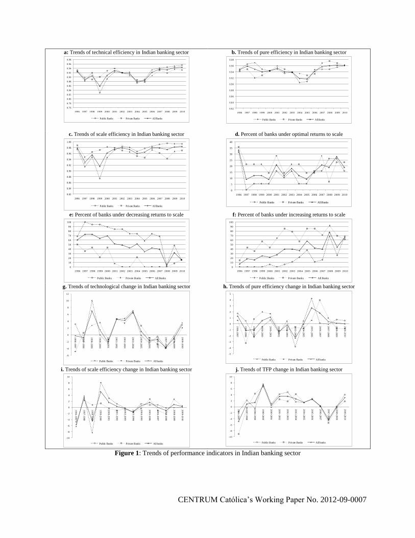
CENTRUM Católica‟s Working Paper No. 2012-09-0007

a: Trends of technical efficiency in Indian banking sector

0.76

0.78

0.80

0.82

0.84

0.86

0.88

0.90

0.92

0.94

0.96

0.98

1996 1997 1998 1999 2000 2001 2002 2003 2004 2005 2006 2007 2008 2009 2010

Public Banks Private Banks All Banks

b. Trends of pure efficiency in Indian banking sector

0.82

0.84

0.86

0.88

0.90

0.92

0.94

0.96

0.98

1996 1997 1998 1999 2000 2001 2002 2003 2004 2005 2006 2007 2008 2009 2010

Public Banks Private Banks All Banks

c. Trends of scale efficiency in Indian banking sector

0.82

0.84

0.86

0.88

0.90

0.92

0.94

0.96

0.98

1.00

1996 1997 1998 1999 2000 2001 2002 2003 2004 2005 2006 2007 2008 2009 2010

Public Banks Private Banks All Banks

d. Percent of banks under optimal returns to scale

0

5

10

15

20

25

30

35

40

1996 1997 1998 1999 2000 2001 2002 2003 2004 2005 2006 2007 2008 2009 2010

Public Banks Private Banks All Banks

e: Percent of banks under decreasing returns to scale

0

10

20

30

40

50

60

70

80

90

100

1996 1997 1998 1999 2000 2001 2002 2003 2004 2005 2006 2007 2008 2009 2010

Public Banks Private Banks All Banks

f: Percent of banks under increasing returns to scale

0

10

20

30

40

50

60

70

80

90

100

1996 1997 1998 1999 2000 2001 2002 2003 2004 2005 2006 2007 2008 2009 2010

Public Banks Private Banks All Banks

g. Trends of technological change in Indian banking sector

-6

-4

-2

0

2

4

6

8

10

12

19

96

-19

97

19

97

-19

98

19

98

-19

99

19

99

-20

00

20

00

-20

01

20

01

-20

02

20

02

-20

03

20

03

-20

04

20

04

-20

05

20

05

-20

06

20

06

-20

07

20

07

-20

08

20

08

-20

09

20

09

-20

10

Public Banks Private Banks All banks

h. Trends of pure efficiency change in Indian banking sector

-5

-4

-3

-2

-1

0

1

2

3

4

5

19

96

-1997

19

97

-1998

19

98

-1999

19

99

-2000

20

00

-2001

20

01

-2002

20

02

-2003

20

03

-2004

20

04

-2005

20

05

-2006

20

06

-2007

20

07

-2008

20

08

-2009

20

09

-2010

Public Banks Private Banks All banks

i. Trends of scale efficiency change in Indian banking sector

-10

-8

-6

-4

-2

0

2

4

6

8

10

19

96

-19

97

19

97

-19

98

19

98

-19

99

19

99

-20

00

20

00

-20

01

20

01

-20

02

20

02

-20

03

20

03

-20

04

20

04

-20

05

20

05

-20

06

20

06

-20

07

20

07

-20

08

20

08

-20

09

20

09

-20

10

Public Banks Private Banks All banks

j. Trends of TFP change in Indian banking sector

-10

-8

-6

-4

-2

0

2

4

6

8

10

19

96

-1997

19

97

-1998

19

98

-1999

19

99

-2000

20

00

-2001

20

01

-2002

20

02

-2003

20

03

-2004

20

04

-2005

20

05

-2006

20

06

-2007

20

07

-2008

20

08

-2009

20

09

-2010

Public Banks Private Banks All banks

Figure 1: Trends of performance indicators in Indian banking sector