Embed Size (px)
Citation preview

© Milad Moradi, 2020
Evaluating the quality of OSM roads and buildings in the Québec Province
Mémoire
Milad Moradi
Maîtrise en sciences géomatiques - avec mémoire
Maître ès sciences (M. Sc.)
Québec, Canada

Evaluating the Quality of OSM Roads and Buildings in the Québec Province
Mémoire
Milad Moradi
Sous la direction de :
Stéphane Roche, directeur de recherche
Mir Abolfazl Mostafavi, codirecteur de recherche

ii
Résumé
Ces dernières années, de nouvelles méthodes de collecte de données géospatiales basées sur la
contribution du public se sont développées. L’information géographique volontaire
ou « Volunteered Geographic Information (VGI) » en anglais, renvoie à des contextes dans lesquels
les citoyens génèrent volontairement du contenu géospatial et le partage avec le reste de la
communauté. OpenStreetMap est l'un des projets VGI les plus réussis. Il vise à créer une carte du
monde modifiable et gratuite. Les citoyens peuvent participer à ce projet en créant de nouvelles
fonctionnalités, en modifiant celles existantes ou en ajoutant des valeurs d'attribut aux objets
cartographiés. Les valeurs d'attribut sont stockées dans la base de données OSM sous forme de
paires «clé = valeur». Il existe trois façons de participer à OSM: numériser des images aériennes,
importer des coordonnées GPS ou importer un ensemble de données. Aucune expertise en
géomatique ou SIG n'est requise pour participer au projet. De plus, il n'y a pas de règle prédéfinie
pour le balisage et les participants OSM peuvent ajouter n'importe quelle clé ou valeur aux
fonctionnalités. Par conséquent, il existe de réelles préoccupations concernant la qualité des
données OSM. Cette recherche évalue la qualité de la base de données OSM sur la base des
éléments de qualité mentionnés dans la norme ISO (ISO 19157: 2013). En raison de l'accès limité
aux ensembles de données de référence, seules l'exhaustivité, la précision de la position, la précision
des attributs et la précision de la forme géométrique sont évaluées dans cette recherche. Dans un
premier temps, toutes les mesures proposées pour évaluer la qualité des données spatiales sont
passées en revue. Ensuite, la qualité des bases de données des routes et des bâtiments OSM est
évaluée à l'aide de ces mesures. Enfin, une analyse statistique est effectuée pour mesurer la
corrélation entre les mesures de qualité et les indicateurs de qualité potentiels tels que la densité
de la population, le niveau de revenu et la distance au centre de la ville. Ces indicateurs peuvent
fournir un aperçu de la qualité des données OSM lorsqu'aucune donnée de référence n'est
disponible.

iii
Abstract
In the recent years, a new method of spatial data collection based on the public participation has
emerged which is called Volunteered Geographic Information (VGI). In VGI projects, citizens
voluntarily generate spatial content and share it with the rest of the community. OpenStreetMap is
one of the most successful VGI projects that aims to create an editable, free map of the world.
Citizens can participate in this project by creating new features, editing the existing ones or adding
attribute values to the features. Attribute values are stored in OSM database as “key=value” pairs.
There are three ways of participating in OSM: digitizing aerial images, importing GPS coordinates
and importing a data set. No expertise in geomatics or GIS is required for participating in the project.
Furthermore, there is no pre-defined rule for tagging and OSM participants can add any key or value
to the features. Consequently, there are real concerns regarding the quality of OSM data. This
research, propose to assesse the quality of OSM database based on the quality elements that are
mentioned in ISO standard (ISO 19157:2013). Due to the limited access to reference data sets, only
completeness, positional accuracy, attribute accuracy and shape accuracy are evaluated in this
research. In the first step, all the measure that are proposed for assessing the quality of spatial data
are reviewed. Then, the quality of OSM roads and buildings databases are assessed using these
measures. Finally, the statistical analysis is done to measure the correlation between quality
measures and potential quality indicators such as population density, incomelevel and the distance
to the center of the city. These indicators can provide an insight into the quality of OSM data where
no reference data is available.

iv
Table des matières
Résumé ............................................................................................................................................................... ii
Abstract ............................................................................................................................................................... iii
Table des matières ............................................................................................................................................. iv
Liste des Figures ............................................................................................................................................... vii
Liste des Tableaux .............................................................................................................................................. ix
Liste des abréviations, sigles, acronymes ........................................................................................................... x
Remerciements ................................................................................................................................................... xi
Introduction ......................................................................................................................................................... 1
Research Questions ........................................................................................................................................... 2
Research Objectives ........................................................................................................................................... 3
Steps of the research .......................................................................................................................................... 4
Literature Review ............................................................................................................................... 7
Volunteered geographic information ............................................................................................................... 7
VGI and related concepts ........................................................................................................................... 8
Different types of VGI ................................................................................................................................. 9
VGI Applications ....................................................................................................................................... 10
Spatial Data Quality ...................................................................................................................................... 10
VGI quality................................................................................................................................................ 13
OpenStreetMap ............................................................................................................................................ 15
OSM Data Structure ................................................................................................................................. 16
Motivation of Contributors ........................................................................................................................ 18
Tools to Edit or Work with OSM Data ....................................................................................................... 19
OSM Data License ................................................................................................................................... 20
Humanitarian OSM ................................................................................................................................... 20
OSM data quality .......................................................................................................................................... 20
The Quality of OSM Roads ...................................................................................................................... 23
The Quality of OSM Buildings .................................................................................................................. 25
Evaluating the Quality of OSM Roads .............................................................................................. 29
Introduction ................................................................................................................................................... 29
OpenStreetMap Quality Assessment ........................................................................................................... 31
Spatial Data Quality ................................................................................................................................. 31

v
VGI Data Quality ...................................................................................................................................... 32
OSM Data Quality .................................................................................................................................... 33
Quality Indicators ..................................................................................................................................... 34
Materials and Methods ................................................................................................................................. 35
Evaluating Completeness ........................................................................................................................ 35
Evaluating Positional Accuracy ................................................................................................................ 36
Evaluating Attribute Accuracy .................................................................................................................. 39
Evaluating the Quality of OSM ..................................................................................................................... 40
Study Area ............................................................................................................................................... 40
Data ......................................................................................................................................................... 40
Completeness .......................................................................................................................................... 42
Positional Accuracy .................................................................................................................................. 44
Attribute Accuracy .................................................................................................................................... 51
Statistical Analysis ................................................................................................................................... 54
Conclusion .................................................................................................................................................... 58
Evaluating the Quality of OSM Buildings .......................................................................................... 60
Introduction ................................................................................................................................................... 60
Methodology ................................................................................................................................................. 62
Feature Matching ..................................................................................................................................... 62
Completeness .......................................................................................................................................... 70
Positional accuracy .................................................................................................................................. 72
Shape accuracy ....................................................................................................................................... 73
Attribute accuracy .................................................................................................................................... 75
Implementation ............................................................................................................................................. 75
Study area ................................................................................................................................................ 75
Data ......................................................................................................................................................... 78
Preprocessing .......................................................................................................................................... 79
Feature Matching ..................................................................................................................................... 82
Evaluating the completeness ................................................................................................................... 82
Evaluating the positional accuracy ........................................................................................................... 87
Evaluating the shape accuracy ................................................................................................................ 90
Evaluating the attribute accuracy ............................................................................................................. 96
Statistical analysis .................................................................................................................................... 97

vi
Conclusion .................................................................................................................................................. 105
Conclusion ...................................................................................................................................................... 106
Bibliographie ................................................................................................................................................... 111

vii
Liste des Figures
Figure 1. the steps of the research ..................................................................................................................... 6
Figure 1-1. The flow of information in Web 2.0 ................................................................................................... 7
Figure 1-2. Overview of the components of the geographic data quality ([7]) ................................................... 11
Figure 1-3. OpenStreetMap website ................................................................................................................. 15
Figure 1-4. The number of OSM registered users over the time (Source: [47]) ................................................ 16
Figure 1-5. Distribution of values for the key "highway" (Source [54]) .............................................................. 18
Figure 1-6. Market share of each OSM editor tool ( Source: [13]) .................................................................... 19
Figure 2-1. average distance between the two lines (Source: [90]) .................................................................. 36
Figure 2-2. Hausdorff distance between two lines (inspired from: [90]) ............................................................ 37
Figure 2-3. The increasing buffer method (source: [64]) ................................................................................... 38
Figure 2-4. Double buffer method (Source: [91]) .............................................................................................. 39
Figure 2-5. reference roads (left) and the OSM roads (right) [95] ..................................................................... 41
Figure 2-6. The two data sets in the campus of Laval University [95] ............................................................... 42
Figure 2-7. The completeness of OSM road network. 1- Left: Old Québec 2- Right: outside urban areas ...... 43
Figure 2-8. The completeness of OSM road network in the province of Québec [95], [97] ............................... 44
Figure 2-9. An example of increasing buffer method for the distance of 2 m .................................................... 45
Figure 2-10. The positional accuracy of the OSM road network using increasing buffer method ..................... 46
Figure 2-11. The positional accuracy of each type of road ............................................................................... 47
Figure 2-12. Positional accuracy of OSM roads calculated using IBM with 1m, 2m and 5m buffers ................ 48
Figure 2-13. An example of double buffer method ............................................................................................ 49
Figure 2-14. Positional accuracy of the OSM roads calculated by double buffer method using 1m buffers ..... 50
Figure 2-15. Value of Levenshtein distance for the whole province of Québec ................................................ 52
Figure 2-16. The Levenshtein distance calculated for each grid ....................................................................... 53
Figure 2-17. Levenshtein distance for each grid around Québec city ............................................................... 54
Figure 3-1. The issues regarding matching OSM building footprints with reference ones ................................ 65
Figure 3-2. The errors of matching OSM building footprints with reference ones ............................................. 66
Figure 3-3. Polygon aggregation for feature matching ...................................................................................... 68
Figure 3-4. Proposed feature matching algorithm ............................................................................................. 69
Figure 3-5. The study area ................................................................................................................................ 77
Figure 3-6. Cities that are selected as case studies. ........................................................................................ 77
Figure 3-7. Distribution of OSM buildings in the province of Québec ............................................................... 80
Figure 3-8. Reference data and clipped OSM data in Québec City. ................................................................. 81
Figure 3-9. Reference data and OSM data on the campus of Laval University ................................................ 81
Figure 3-10. The 5 measures of quality for each grid in Québec City ............................................................... 86
Figure 3-11 OSM buildings in and in the reference database with their centroids ............................................ 87
Figure 3-12. Average distance between the centroid of the OSM buildings and their corresponding reference
building (m) ....................................................................................................................................................... 88
Figure 3-13. Scatter diagrams of the displacement of the centroids of OSM buildings ..................................... 89
Figure 3-14. Average positional accuracy for each grid cell in Québec City ..................................................... 90
Figure 3-15. Area ratio between the OSM buildings and their corresponding reference building ..................... 91
Figure 3-16. The compactness values for each city.......................................................................................... 92
Figure 3-17. Average Hausdorff distance for each city (m) ............................................................................... 93

viii
Figure 3-18. Average value of the average distance for each city (m) .............................................................. 94
Figure 3-19. Shape accuracy measures for the city of Longueuil ..................................................................... 95
Figure 3-20. taginfo results for the tag "building=yes" (source: https://taginfo.openstreetmap.org/) ................. 96
Figure 3-21. Calculating the correlation between the quality measures and potential indicators ...................... 99

ix
Liste des Tableaux
Table 2-1. The frequent errors that exist in the road names in the province of Québec ................................... 51
Table 2-2. Correlation coefficient between quality measures and potential quality indicators .......................... 55
Table 2-3. Result of Spearman’s correlation test between the quality measures and quality indicators ........... 57
Table 3-1. Cities that are selected for the study area ....................................................................................... 76
Table 3-2. Links to the provider of the reference data for each city .................................................................. 78
Table 3-3. Unit-based completeness for the selected cities in the Québec Province ....................................... 83
Table 3-4. Average area of the building footprints in OSM and in the reference databases ............................. 84
Table 3-5. The object-based completeness assessment for the cities of the province of Québec ................... 85
Table 3-6. Spearman’s rank correlation between the quality measures and quality indicators ....................... 101
Table 3-7 Correlation between the size of the buildings' footprints and quality measures .............................. 103
Table 3-8. Result of Spearman’s correlation test between the quality measures and quality indicators ......... 104

x
Liste des abréviations, sigles, acronymes
GIS Geographic Information System
VGI Volunteered Geographic Information
IBM Increasing Buffer Method
DBM Double Buffer Method
OSM OpenStreetMap
NAD North American Datum
ODbL Open Database License
UGSC User Generated Spatial Content
GDP Gross Domestic Product
GPS Global Positioning System

xi
Remerciements
I want to thank everyone who helped me during this thesis, especially my supervisors and my family.

1
Introduction
In the last two decades, Web 2.0 has changed the way people were interacting with the internet [1]. Before Web
2.0, the information came from the internet servers towards the people, while Web 2.0 technologies enabled
people to produce content and send it back to the server [1]. Therefore, Web 2.0 enabled internet users to share
content among themselves. This new technology is the basic concept behind many famous websites such as
Wikipedia, Tweeter, and Facebook [2]. In the realm of spatial and geographic applications, Web 2.0 enabled
users to share their geographic data or share their spatial knowledge about features and places. On the other
hand, easy access to GPS-enabled devices such as cell phones facilitated the production of geographic content
[3]. Therefore, volunteers can produce geographic content and share it over the internet with other citizens [3].
Volunteered Geographic Information (VGI) is a term introduced by Goodchild to address this new phenomenon
[3]. In a VGI project, citizens contribute voluntarily in producing geographic content and sharing it with the rest
of the citizens. OSM is an example of VGI where volunteers contribute to the project by digitizing new features
from aerial imagery or by editing the semantic attributes of the existing features [4]. Every contributor can add,
edit or remove features from the map. OSM does not ask its contributors to have a certain level of knowledge
about geographic data [5]. Any non-expert person can join the project. Therefore, there is a debate about the
quality of OSM data. Even some cases of vandalism (introducing error to map intentionally) have been detected
by researchers [6].
The quality of spatial data is very important. Practically, it is impossible to use a database properly for an
application without having knowledge about its quality. It is the quality of the data that determines whether it is
fit for a purpose or not. ISO standard (19157) [7] mentions six elements of quality: 1) completeness, 2) positional
accuracy 3) semantic accuracy, 4) logical consistency, 5) temporal accuracy and 6) fitness for use. This standard
defines a unique way of understanding the quality of spatial data. Several quality measures are proposed to
measure these elements of quality. There are different measures (e.g. shape, area, et.) for evaluating the
positional accuracy of polygonal, linear, and other types of features. This research first finds different measures
of quality proposed by previous researche works. Then, it evaluates the quality of OSM data in the province of
Québec using these measures.
GenerallytThese measures of quality are calculated by comparing the OSM data to a reference database. This
method of quality assessment cannot be used in the regions where no reference data is available (does not exist
or is expensive). Thus, researchers proposed other indicators of quality [8] without using those meseurs.
Indicators can describe the quality where no other method of quality assessment is available. Population [8],
income [9] density of OSM buildings [10] can be used as indicators that have been proposed by previous

2
researches. The correlation between indicators and measures of quality is calculated in this research to provide
knowledge about each indicator and their relations with the elemnets of data quality.
Research Questions
OSM data is freely available for users and they just must mention the source of the data. In addition, it is not
possible to use geographic data properly in any application without having complete information describing the
quality of the geographic data. The data of OSM is available, but the quality of this data is not very well
investigated so far. The first question of this research is:
• How is the quality of OpenStreetMap road and building data in the province of Québec?
o How complete is the data?
o How is the attribute accuracy of the data?
o How is the positional accuracy of the data?
o How is the shape accuracy of the data?
To answer this question, we must evaluate different measures of the quality of OSM data in the province of
Québec. Quality is not a clear concept and in different applications, it may be defined in different ways. In terms
of spatial data quality, a standard is published by ISO, and this research follows this standard to evaluate the
quality of OSM data.
Different quality measures are proposed by researches to evaluate different aspects of quality. Thus, it is
necessary to do a literature review and find the most efficient measures proposed by the previous researches.
The second question of this research is:
• Which measures of quality should be used to evaluate the quality of OSM roads and buildings?
The main objective of OSM is to provide a free and open map of the world for the places where authoritative
data is not available, or it is not free. The traditional methods of quality evaluation compare the test database to
a reference database, but these methods are not suitable for OSM quality assessment in the places where no
authoritative data is available. Thus, researchers tried to find indicators that can describe the OSM data quality
in those places. This research tries to expand these indicators and asses their correlation with quality measures
in order to determine which indicator has a relationship with each quality measure. These quality indicators are
extracted from the previous researches. However, previous researches did not evaluate the relationship (positive

3
or negative correlation) between each indicator and all quality measures. Thus, the knowledge in this area is not
comelete. This research will fill the gaps of previous researches by doing a complete evaluation of the
relationship between quality measures and quality indicators. For example, if a variable (such as population) is
proved to have a positive association with a quality measure (such as completeness), this research investigates
the following hypothesis: “This variable (quality indicator) has a positive correlation with other quality measures
such as positional accuracy and attribute accuracy”. The variables that are proved to have a positive correlation
with a quality measure, are called a quality indicator or a proxy for that measure. These quality indicators can
potentially have a positive correlatyion with other measures of quality. Thus, the last question of this research
tries to provide knowledge about the relationship between quality indicators and the quality measures that are
not evaluated in the previous researches.
The third question of this research is:
• What is the relationship (correlation value) between the potential quality indicators and quality
measures?
The answer to this question provides insight into the use of quality indicators and their role in the quality
assessment of the OSM database.
Research Objectives
The quality assessment of OSM is an important chalange that provides knowledge about the fitness of OSM
roads and buildings data for different applications. Spatial data quality is not a well-defined concept and there is
a debate about it. In addition, VGI (and especially OSM) is very common these days and a wide range of people
contribute to VGI projects such as OSM. The data produced by these people cannot be used properly, unless
we have a good understanding of the quality of this new data source. Therefore, it is very important that
researchers develop methods that can provide knowledge about the quality of OSM. Hence, the first objective
of this research is:
• Identifying measures proposed in the literature for evaluating the quality of OSM linear (roads)
and polygonal (buildings) data.
When the proposed methods are analyzed, the suitable ones will be selected to evaluate the quality of OSM
roads and buildings data in the province of Québec. OSM project has a variety of active contributors in the
province of Québec and it is important to evaluate the quality of this data in order to be able to use it in appropriate
applications.

4
The second objective of this research is:
• Evaluating the quality of OSM roads and buildings data in the province of Québec using the
measures that are discussed in the previous step.
Considering the fact that the traditional methods of quality assessment that compares the OSM data with the
reference data are not suitable for the places where no authoritative data is available, this research analyses
the correlation between a number of potential quality indicators (such as population, income, distance from the
center of the city, …) and quality measures. These correlations will provide information about the potential quality
indicators. I call them potential quality indicators, because even though previous researches proved a positive
correlation between them and a specific quality measure, they may or may not have a positive correlation with
other quality measures. The results of the correlation analysis will tell us which indicator can better describe
each quality measure. Which indicator is stronger or which one of these potential indicators are not suitable (if
the correlation is low).
The third objective of this research is:
• Calculating the correlation between the quality measures and the potential quality indicators in
order to find out which one of these potential indicators can be used for describing the quality.
This step requires calculating the quality measures and quality indicators for each region of the case study.
Then, calculating the correlation between these two groups of variables to understand the role of each of them
in describing the quality.
Steps of the research
In this research, the first step is finding the previous researches that have been done about the quality
assessment of OpenStreetMap data. The purpose of this literature review is to find out 1) which methods have
been proposed for quality assessment and which quality measures are proposed to provide a quantitative
evaluation of OSM data quality 2) which potential quality indicator is proposed by the previous researches.
Therefore, the output of this step is two lists: 1) a list of measures of quality 2) a list of potential quality indicators.
In the next steps, the road data is downloaded from OSM and authoritative sources. The downloaded data is
preprocessed to remove the road types that do not exist in the authoritative database (such as step ways). The
preprocess step deletes the buildings that are smaller than 40 square meters because most probably they are
garages and other small buildings that look like houses in aerial images. When the data from both sources is
ready, feature matching algorithms are used to find corresponding features in order to enable comparison

5
between them. In the case of buildings, the authors proposed a new feature matching algorithm that is based
on the percentage of overlap and shape similarity of the two polygons.
Next, the measures of quality that are listed in the previous step are calculated for OSM roads and buildings
database. Completeness, attribute accuracy, shape accuracy and positional accuracy are the elements of the
quality that are evaluated in this research. In the next step, the value of the potential quality indicators is
calculated. This research takes into account 7 quality indicators: population, income, the density of OSM
buildings, the density of OSM roads, the number of POIs, the distance to the center of the city, and the size of
the buildings. The size of the buildings cannot be used for roads but the rest of the quality indicators are
measured for both roads and buildings.
Finally, the correlation between the quality measures and quality indicators is evaluated to find out the
relationship among them. A high correlation shows that the quality measure can be described with the indicators,
while a low correlation shows that it is impossible to describe the behavior of the quality measures with the help
of quality indicators.
Because roads are linear features and buildings are polygonal features, the author decided to separate these
two different processes in two chapters. Thus, the rest of this research consists of these chapters: 1) literature
review 2) quality assessment of roads 3) quality assessment of buildings 4) conclusion.

6
Figure 1. the steps of the research

7
Literature Review
Volunteered geographic information
In recent decades, citizens are not only the users of the data, but they are also the providers of it [11]. By the
advent of Web 2.0, which is also known as the participatory Web, the users of the Internet became able to
produce content and participate in the flow of information [2]. Websites based on Web 2.0 allow their users to
participate in the community and build a virtual community in which each member can produce and share content
with other members [2]. Examples of this participation include tagging, writing a comment, sharing a video, and
sharing a document [2]. In other words, before Web 2.0, the flow of information was from providers to users, but
after Web 2.0, users also can produce and share content [3]. Figure 1-1 illustrates the flow of information in Web
2.0. Popular websites such as Wikipedia, Facebook, and Youtube are examples of Web 2.0 [2].
Figure 1-1. The flow of information in Web 2.0
This new concept of Web 2.0 revolutionized the traditional geographic information collection methods and
enabled a phenomenon that is called VGI by Goodchild [3]. Goodchild believes that VGI can be considered as
a democratization of GIS because it provides free access to spatial data for all citizens [12]. He argued that by
the advent of Web 2.0, the flow of information between the user and server became a two-way road [3]. From
the point of view of Goodchild, two main factors facilitated the growth of VGI over the recent years: 1) the
facilitation to share geographic data, 2) the facilitation to collect geographic data [3]. The facilitation in sharing
the geographic data happened by Web 2.0, while the facilitation to collect the geographic data happened due to
the GPS devices and cameras [3]. Therefore, today citizens are able to use their cellphone to collect geographic

8
data and then use Web 2.0 to share it with others. The cellphones also enable users to collect photos, and
thanks to the GPS devices, these photos can be tagged with geographic coordinates [3]. These geo-tagged
photos are a source of geographic data that can be shared easily using Web 2.0 technologies. Overall, the new
technologies allow human beings to act as sensors and collect geographic data in different forms and share it
with others, a phenomena that Goodchild referred to it as “citizens as sensors” [3].
Therefore, in the domain of VGI, there are different concepts, such as citizen science, user-generated content,
and public participatory GIS. These concepts will be discussed in detail in the next section.
VGI and related concepts
Citizen science
As discussed earlier, Goodchild introduced the concept of VGI, and explained that in recent years, thanks to the
technological advances, humans can act as sensors and collect and share geographic information with other
members of the community [3]. The term citizen science is then used to describe the act of any group of citizens
who work as observers and collect data to solve any specific problem in the world [3]. Therefore, VGI can be
related to citizen science because in VGI, citizens are observers, and they detect a specific phenomenon, and
they report it to the rest of the community. For example, a GIS website that allows citizens to report information
about a wildfire or specific animal’s nests are two examples of the application of VGI in citizen science. Another
example can be a system that allows users to upload their trajectory and then use those trajectories to monitor
the traffic. In fact, any geographic information that is collected by volunteers to study any specific issue is a case
where VGI can be used in citizen sciences [13].
User-generated Content
User-generated content is referred to a content or information such as text, photo, or document that is shared
by users of online platforms such as wikis [14]. The rise of user-generated content happened at the same time
web 2.0 allowed users to share their content [14]. The social media are a good example of platforms where
users produce content and share it over the web. Usually, there is a community where the users belong, and
they publish their content to share with the rest of the members of the community [14]. Internet forums, blogs,
and wikis are the most famous places where user-generated content is shared [14]. Usually, a pool of information
is created in these communities [13]. The geographic data that contributors to OpenStreetMap produce is a good
example of user-generated content in the GIS world [13]. Therefore, user-generated spatial content is a specific
type of user-generated content that should be considered [1][13]. Some criticism of user-generated content,
such as data quality, is even more serious in spatial applications because they have been collected by non-
expert members of the community [13]. Considering the fact that user-generated content is collected by a variety
of users, the produced content is not necessarily consistent [15]. Thus, an important effort should be made to

9
process the user-generated content before being able to use it properly [15]. [1] believes that in terms of VGI,
user-generated content can provide us with the ability to supply information and update them on a regular basis
for existing databases. [1] mentioned that the geotagged photos of Flickr are a good example of user-generated
spatial content that can be a source of useful information for updating existing databases . In terms of VGI, the
generated content and the order in which the content is generated (places that are mapped) can indicate the
priorities and interests of the contributors [16].
Crowdsourcing
Based on Lexico’s dictionary (powered by Oxford), crowdsourcing is getting a task done by a variety of people
either paid or not [17]. In fact, crowdsourcing is outsourcing a task or a series of tasks to the crowds of people
who may do it as part of a contract or just as a volunteer service [18]. Wikipedia defines crowdsourcing as a
model of sourcing in which some services or information or other kinds of products are delivered to a company
or organization by using the ideas, expertise, and finances of a large group of people [19]. The major difference
between outsourcing and crowdsourcing is that in crowdsourcing, the task is done by a large group of citizens,
while in outsourcing, the task can be done by any individual [19]. Internet is usually used to distribute the task
and information among the community, and as a consequence, crowdsourcing increased by the growth of the
Internet and its accessibility [19]. One of the challenges of the crowdsourcing of spatial data is to collect different
results and put them together to make a unique, consistent final product [20]. Crowdsourcing spatial data has
been successfully applied in a number of domains, including disaster management, tourisem, and etc. [21].
Different types of VGI
VGI can be classified based on the type of information that it provides. From this point of view, there are three
main classes, including text-based, image-based, and map-based VGI [22]. For example, geo-tagged
microblogs such as geotagged tweets, geo-tagged images in Flickr, and similar services and geo-tagged videos
are different types of VGI [22]. The online platforms that allow the contributors to draw map features and add
attributes to them are considered as the map-based VGI [22], [23]. In map-based VGI, the contributors contribut
directly to creat or modify the geographic features or add new attributes to existing features [22]. Thus, in map-
based VGI, in general, the geographic part of the contribution is more considerable, and usually, the contributors
are implicitly contributing to generating geographic content [22], [23]. In text-based VGI, however, the attributes
or the geographic information is usually achieved by text mining methods or direct contribution of the citizens
[22].
VGI data can be classified from different point of views. One of the differences between VGI and user-generated
spatial content is that in the case of VGI, the participation of the user in the generation of the content should be
voluntarily [24]. Therefore, the applications that collect the trajectory information from cellular phones without

10
the direct intention of the person may not be considered as VGI. Generally, VGI can be categorized in 2 different
cases: explicitly volunteered and implicitly volunteered data [24]. A tweet that is an example of explicit
volunteered information and the information that people add to OSM is explicitly volunteered information [24].
VGI can further be categorized into groups based on the fact that whether or not the geographic data is explicit
or implicit. For example, a tweet that talks about a specific place is a geographically implicit information, while a
tweet that is geo-tagged is an explicit information [24]. In VGI, human acts as a sensor, depending on active or
passive sensing; the type of VGI can be categorized [24].
VGI Applications
Considering the fact that VGI provides an extensive amount of freely available geographic information, it can be
used in a wide range of applications and improve the traditional tools and techniques. VGI has been successfully
used for humanitarian purposes. In the case of earthquakes, OpenStreetMap data is used to help the search
and rescue teams in the regions where no authoritative data were available [25]. In addition, VGI is used for
disaster management [26]–[28] and intelligent transportation [29], [30]. VGI has been used to evaluate public
opinion about the large scale projects [25]. It is also used for mapping mental and contagious diseases in urban
areas [31]. VGI can be used as a way of studying global mobility patterns [32]. Map-based VGI can be used for
a variety of purposes. Practically, all the purposes that need geographic data. For example, OSM data is used
in urban planning [25]. Map-based VGI is also used for facilitating the routing of the people with motor disability
[33]. In addition, VGI can be used for land-use modeling [34]. It can be concluded that VGI is a valuable source
of information, even though extracting the useful information from the flow of VGI needs precise modeling and
tools.
Spatial Data Quality
Lexico’s dictionary (powered by Oxford) defines quality as “The standard of something as measured against
other things of a similar kind; the degree of excellence of something” [35]. Quality assessment is an essential
part of any process. In terms of geographic data, various researches have been undertaken to define the quality
of geographic data. Geographic data cannot be used properly in different applications unless its quality is
measured in a standard and measurable way. Therefore, in the 1980s the discussion about the quality of
geographic data increased in the US Federal Government and some other universities [18]. These discussions
resulted in a consensus of the researchers over 5 principal elements of geographic data quality, including
positional accuracy, attribute accuracy, logical consistency, completeness, and lineage [18]. The quality of
geographic information should be described in a way that it can have the same meaning for all the producers
and users of the data because if the quality is not expressed in a unique standard way, then it can make
confusion. International Organization for Standardization (ISO) tried to address this need and published a

11
standard for the quality of geographic data [7]. Figure 1-2 describes the components of the spatial data quality
based on ISO 19157:2013 standard. Based on this standard, there are six elements of quality, and for each
report of quality, these six elements should be discussed [7].
Figure 1-2. Overview of the components of the geographic data quality ([7])
The elements of quality described by ISO 19157 standard are: completeness, logical consistency, positional
accuracy, thematic accuracy, temporal quality and usability [7]. Completeness is an element that evaluates the

12
presence and absence of the geographic features or their attributes from the database [7]. If there are some
extra features in the database, commissions are occured, while if there are some missing features, omissions
happens in the database [7]. Completeness consists of two parts: data completeness and model completeness
[36]. Data completeness refers to the relation between the features in the data set and the features in the real
world, while model completeness refers to the degree to which the model that describes the application needs
is complete [36].
Logical consistency evaluates whether or not the data is in line with the rules and structures [7]. Based on ISO
19157, standard logical consistency consists of four parts: conceptual consistency, domain consistency, format
consistency, and topological consistency [7]. It describes how well attributes, relations, and features are in line
with data specifications [36]. Evaluation of logical consistency depends on the data structures and models that
describe the nature of the data [36].
Positional accuracy refers to the accuracy of the position of the features on the map in comparison to the reality
[7]. Due to the fact that determining the position of the features on the surface of the Earth is done by a set of
measurements, the calculated coordinates will never be exactly correct [18]. The positional accuracy of the
features of the map is determined by equipment used, operator policy, digitization policy, and source material
[36]. In order to evaluate positional accuracy, the position of the feature should be compared to its “true” position
on the surface of the Earth [36]. Positional accuracy follows the rules of error propagation [36]. Numerical
assessment of positional accuracy is easier than other quality elements because it is related to coordinates that
are by nature numeric. Root mean square average is a frequently used method for evaluating the positional
accuracy of features [36].
Thematic accuracy refers to the degree of correctness and accuracy of the attributes that describe geographic
features [7]. In the ISO standard, temporal accuracy refers to the accuracy of the temporal attributes and the
accuracy of the time measurements [7]. Temporal information describes the date of data acquisition, the time of
the last update, and the period in which the data is considered valid [36]. Information about creation, modification,
and deletion of features should be evaluated in temporal quality assessment [36].
ISO standard considers usability as the last element of data quality [7]. Usability is defined and measures based
on the different needs and requirements of the user in each application [7]. Thus, usability is not defined for each
dataset, but it is defined based on the application that the dataset is used for. In fact, this element of ISO standard
refers to the concept that is called “fitness for use” by other researchers [37]. This concept is related to the fact
that the quality of data should always be evaluated in relation to the application because a data set that is not
qualified for one application may be qualified enough for another application. Thus, without considering the
application, evaluating the quality is not complete.
13
There is another classification for spatial data quality that believes that there are two main categories of quality:
internal quality and external quality [5], [37], [38]. External quality of the data refers to the “fitness for use” of
data in the specific application that the data is going to be used [5]. On the other hand, internal quality
assessment explores the degree to which the data is in line with the rules and predefined specifications [5]. In
fact, ISO standard refers to 5 internal quality elements, and the sixth quality element is usability that refers to
the external quality assessment. External assessment of quality depends on the application and requirements
of the user, while internal quality is independent of application [37]. External quality also is referred to as “fitness
for use” of the data set for a specific application [37]. Internal quality depends on the quality of measurement
equipment, the degree to which the data meets the standards, and how well the data is in line with the data
structures and other criteria [5].
VGI quality
As mentioned in the previous sections, the advent of Web 2.0 enabled the citizens to produce content and share
it over the internet. An important part of this content has a geographic nature. In recent years, thanks to the
growth of the internet and other technologies, citizens are more and more involved in the process of geographic
content production [18]. Traditionally, geographic content is produced by organizations and governments that
follow specific rules and guidelines [10]. Quality assurance in mapping organizations is enabled in two ways:
quality control rules and procedures to ensure that measurement is precise, taking some samples from the
produced maps, and comparing it to the reference sources [18]. However, these days a large percentage of
geographic content is produced by the individuals who are not necessarily familiar with GIS and spatial data
quality concepts [10]. Thus, a serious concern regarding VGI is the quality of the user generated content because
the majority of VGI is generated by non-specialists who are not following any specific guidelines for quality
control [39].
A percentage of VGI is simply created by digitizing aerial images with volunteers who are not even familiar with
the neighborhood, a phenomenon that is called “armchair mapping” [4], [40], [41]. The fact that non-expert,
armchair mappers are participating in VGI, causes a huge concern about how we can trust VGI and use it in
different applications [10]. Therefore, various researches have been done to evaluate the quality and credibility
of VGI data.
[18] proposed three main quality control mechanisms for VGI including crowdsourcing, social and geographic
methods. These three mechanisms are not dealing with evaluating the quality of the generated content, but they
are general ways to ensure that the production will work well. The reason that we need to develop new methods
for evaluating the quality of VGI is that first, the production rate of VGI is so high, and traditional quality control

14
methods are not efficient. theirdly, there is a great difference in the nature of the methods of data production in
VGI and in traditional ways of collecting geographic data.
Crowdsourcing means solving a problem by referring it to a vast number of volunteers [18]. Thus, we depend
on the wisdom of the crowds to collect the information by sensing the environment [18]. The crowd can not only
generate the information, but they can also detect the errors in the content [18]. This feature of the crowdsourcing
is, by nature, a mechanism of quality control [18]. This phenomenon is a famous fact in computer science that
expresses that if there are enough contributors to a citizen science project, the bugs and errors are automatically
detected and corrected by the community memebers [42]. Therefore, crowdsourcing is both the mechanism of
data collection and quality control [18]. In the case of OpenStreetMap, the contributors detect and correct the
features or the parts of the map that they believe are wrong. If a great number of them work on the neighborhood
of the map, it can be expected that the errors are detected and corrected by the contributors.
The second mechanism proposed by [18] for quality assurance of VGI is a social approach. This mechanism is
also called the “hierarchy of trusted individuals” that control the content that is generated by others [18]. Based
on this mechanism, a group of senior members of the community should supervise the procedures and the
content that is produced by the other members [25]. Then, the data should be verified and accepted by the elite
group before publishing it on the internet [18]. This method is applied in a number of online communities, such
as Wikipedia and OSM [18]. This group of expert users can prevent the occurrence of errors and even vandalism
[6].
The third mechanism of VGI data quality assurance is the geographic approach [18]. Based on the geographic
approach, there are a set of rules and syntaxes that the geographic features follow [18]. Thus, by checking those
rules in the generated content, we can ensure that errors are detected and removed from the database [18]. For
example, a geographic rule about an island is that it should be surrounded by water. Therefore, these rules
should be defined, and the validity of the new content should be verified by those rules. [43] used a spatial data
mining approach to find the geographic rules inside the authoritative data sets. They used an automatic rule
detection algorithm to find the topological relations and rules among different features of the map [43]. Then,
they extracted the rules for forests, parks, and meadows to verify the newly generated content with the previous
rules [43]. [43] is an example of using geographic mechanisms for validating the quality of VGI.
In addition, [11] believes that the credibility of VGI is an issue that needs extensive research because there is a
lot of information about the traditional sources of spatial data, while about VGI data credibility, there are not
enough research. In addition, [11] argues that considering that VGI is a new and relatively fast-changing market,
there is a need to investigate the credibility of VGI. One possible definition for credibility is the accuracy of the
information in its traditional meaning [11]. [11] believes that it is essential that the wisdom of academic crowds

15
be used for evaluating the credibility of the geographic data that is produced by the networks of volunteer
citizens.
OpenStreetMap
OpenStreetMap is an online project that aims to provide the resources for volunteers to participate in the process
of mapping the world and, in the end, to provide a freely accessible map of the world [44]. The purpose of this
project is to provide free geographic data of the world that are updated with the help of the volunteers [44].
OpenStreetMap can be considered as a map-based geographically explicit type of VGI [44]. This project started
in the University College London (UCL), where Steve Coast, the founder of OSM, studied [45]. OSM started its
work in 2004, and since then, it is continuously growing in terms of the amount of information that is stored in its
database [45]. OSM provides users with tools to edit the map and add and remove features [45].
Figure 1-3. OpenStreetMap website
The fact that Bill Clinton, former president of the USA, decided to provide free access to GPS data in 2000,
improved the methods of data collection by GPS receivers [45]. OSM uses GPS receivers as a method of data
collection. GPS trajectories can be used to map the roads. OSM has three main sources of data including:
digitizing aerial images, processing GPS tracks, and import of geographic data from authoritative sources [46].
Yahoo has accepted to provide OSM with free base images that enable users to produce geographic content by
digitizing the images [46]. Unfortunately, there is no way to understand how each geographic feature is added
to the map (by digitizing, GPS, or upload of authoritative organizations) because OSM does not save this kind
of information in its database [5].

16
Contributors of OSM join the project with different motivations. The number of OSM users has been almost
constantly growing over time (2004-2020) except for a few occasions when a number of contributors decided to
withdraw from the project because of different reasons [47]. [48] realized that events could affect withdrawal
rates from the project. For example, when the British national mapping agency released geographic data of the
country freely, it disappointed many contributors to the OSM project [48]. Another event that affected the
withdrawal rate was the license change of OSM [48]. [48] estimated that almost 2000 contributors quit the project
after the license changed.
Figure 1-4. The number of OSM registered users over the time (Source: [47])
[49] evaluated the behavior of the OSM project contributors. They evaluated factors such as the number of
nodes, mean length and sinuosity values of the road network in OSM. By evaluating the data of OSM between
2007 and 2017, they realized that at the beginning, the contributors added the data of main roads such as
highways and motorways. On the other hand, at the end of the period, the residential roads and pedestrian roads
were added [49]. Thus, [49] concluded that the wider roads were mapped before the narrow ones. In addition,
they realized most of the users tend to map short and straight roads rather than long ones [49].
OSM Data Structure
OSM data is used in a wide range of applications. Facebook, Foursquare, Mapquest and Seznam are some
examples of users of OSM data and map [44]. Geographic features (roads, hospitals, …) in the OSM database

17
are stored using a geographic part and an attribute part [50]. The attributes, which are the characteristics of the
objects in the real world, are stored in the database as tags [45], [50]. Each tag represents a characteristic of
the object using key = value pairs. The geographic part consists of three main groups: nodes, ways, and relations
[45], [50]. This model is not following the traditional methods of GIS, where points, lines, and polygons are used
to represent the features [51]. Nodes are simply points that are stored using a pair of coordinates in the WGS84
reference system, and they are useful for storing features without size [5], [44]. On the other hand, ways are
ordered sets of nodes that are used to store linear features (line and polyline if they are open and polygon if they
are closed) in the OSM database [44], [52]. Relations are ordered sets of nodes and ways that are useful for
storing the relations among the features of the map [5], [44], [52]. For example, OSM uses relations to store turn
restrictions for road features in the database [44]. All edits that contributors are doing in the database of OSM
are stored in a PostgreSQL database (which is an open-source database) with PostGIS extension [44]. PostGIS
is an open-source extension for PostgreSQL that enables storing spatial data such as point lines and polygons.
In addition, PostGIS provides a variety of functions for working with these spatial features.
OSM Tags
As mentioned earlier, tags in OSM are simply a “key=value” pairs that represent characteristics of an object in
the real world [45], [50]. The metadata of OSM is stored in the tags [5]. Unlike the geometric part of the object,
the tags can change very frequently [5]. The tags that are assigned to the features are accessible through the
TagInfo (https://taginfo.openstreetmap.org/) service [25]. This service allows the users to find out the most
frequent keys and values that are used in OSM [25].
OSM provides a list of possible key = value pairs for contributors to use in the tagging process of OpenStreetMap
(https://wiki.openstreetmap.org/wiki/Map_Features). This page describes what the difference is between basic
tags and suggests a set of unique tags to increase the uniformity of the map. For example, on this page, there
are guidelines to differentiate between the value of different highway keys such as primary, secondary, tertiary
and residential [50]. Considering the fact that the contributors do not follow these guidelines strictly, there is an
uncertainty about the semantic information available in OSM [53]. For example, maybe one contributor adds
“primary,” and the other one adds “secondary” as the value of the highway key.
Even though OSM provides a list of possible basic tags, the contributors can select any tag that they think is
suitable for describing the object [51]. Thus, there is no restriction for using keys and values for tags in OSM
[45], [51]. There is a huge debate about whether this method of tagging is efficient or not. This free-style tagging
provides freedom for the contributors to add any information to the map. However, there is not enough control
over the tags that contributors use in OSM [45]. [53] believes that this flexibility of the tagging process can cause
a noise in the attributes of the features and an uncertainty about the semantic information of the map.

18
Sometimes one key (such as name) has more than one value. [53] believes that contributors disagreement,
spelling errors, and lack of knowledge about the neighborhood can cause assign of more than one value to a
single key. It is possible that a feature is edited by more than one contributor or more than once by a single
contributor. In this case, if the number of edits on a single feature in OSM is more than a predefined threshold,
the feature is called “heavily-edited feature” or “popular feature” [53]. The number of heavily edited features on
the map is not considerable [53].
Using Taginfo, researchers can explore the tags and have information about the tag content of the OSM
database. Figure 1-5 illustrates the distribution of values for the key “highway” in the whole database of OSM.
Figure 1-5. Distribution of values for the key "highway" (Source [54])
The majority of the features that are tagged by the key “highway” has the value of residential. It means that the
most frequent tag in the database is “highway = residential”. “Service”, “Track” and “Unclassified” are the most
frequent values in the database of OSM.
Motivation of Contributors
Openstreetmap is an online community where a number of citizens gather and contribute to achieving a common
goal [48]. In these online communities, the success of the project depends largely on the contribution of the
members [48]. These contributors have a variety of different reasons and motivations for contribution, and they

19
may withdraw from the community if they lose their motivation [48]. Different studies showed that people have
different motivations to contribute to the OSM project. A number of examples of these motivations are being
interested in providing free information for everyone (data democratization), feeling useful by being part of a
community (OSM community) [45] or having some negative feelings for national mapping agencies who earn
money by selling it to the citizens.
Tools to Edit or Work with OSM Data
Basically, there is no real difference between editing data in OSM or other online communities. However,
considering the fact that OSM contains spatial data, it is necessary that it provides users with tools to create,
edit, and delete spatial features [13]. For example, tools for digitizing roads from aerial images. Or tools to upload
spatial data into the OSM database.
Figure 1-6. Market share of each OSM editor tool ( Source: [13])
Figure 1-6 illustrates the market share of each OSM editor tool. Based on this figure, Potlach and JOSM are the
most frequently used editors on the market. There is not a huge difference among them, and contributors can
select the editor based on personal preferences and the operating system that they use.
The second category of tools of OSM are the tools that are developed for working with OSM data. One of the
most famous open-source tools to work with downloaded OSM data is Osm2postgresql
(https://wiki.openstreetmap.org/wiki/Osm2postgresql). This tool allows users to upload the downloaded OSM
data into a PostgreSQL database with PostGIS extension [56].
OSMPythonTools is an open-source Python library that allows manipulation of OSM data [56]. This library
internally is built based on Pandas and Matplotlib python packages [56]. Moreover, there are a variety of tools
based on R to explore OSM data. These packages include osmar, osmdata R Packages [56]. In addition, several

20
plugins are developed for QGIS, including QGIS OSM Plugin. This plugin can explore both spatial and attribute
values of map features.
OSM Data License
OSM allows everyone to access, download, edit, and use its data freely because the data of OSM is under Open
Database License (ODbL) [57]. This license allows any use of the data as long as it is mentioned that the data
is downloaded from the OSM database, and also, the results of the work are released under Open Database
License (ODbL) [57]. The license of OSM data was not ODbL since the beginning of the project. This license
has changed because the previous license was not suitable for spatial data since it did not allow processing or
combining it with other data [44]. Therefore, on 12 September 2012, the license of the OSM database changed
to ODbL that allows any use of data when the source (OSM contributors) is cited [44].
Humanitarian OSM
OSM is not only a mapping project, but it has a social dimension [57]. For example, in 2010, when the earthquake
happened in Haiti, a group of OSM contributors started to map Haiti [57]. The motivation of this group was to
help search and rescue teams to have maps of Haiti [57]. Therefore, 600 contributors from across the world
helped to provide a map of Haiti in a short time [57]. Finally, the Humanitarian OpenStreetMap Team (HOT) was
created, and in 2013 it was registered as a non-profit organization in the U.S. [57].
OSM data quality
Assessing the quality of the geographic data is necessary before users can use the data in any application.
However, describing the quality of the data is usually difficult and challenging [37]. Without understandable
information about the quality of a data set, there is always a risk of misuse of data [37]. Therefore, one of the
most important issues in quality assessment is assessing “fitness for use” [37]. [37] argues that there are two
main meanings for the “data quality” in the literature. The first category tries to evaluate the quality by evaluating
the presence of errors, which is called “internal quality” [37]. However, the second category tries to evaluate the
quality of data by evaluating how good it answers the needs of the user (external quality) [37].
As mentioned earlier, most of OSM contributors are not necessarily experts in GIS or spatial data collection.
Thus, there are serious concerns about both the internal and external quality of OSM data [58]. It is important to
evaluate the quality of OSM before being able to use it in a specific application. In this section, a literature review
of the research works that deal with the quality of OSM data is provided. Considering the fact that this research
pays attention to the quality of data on roads and buildings, these two data layers are evaluated in separated
subsections.

21
[55] proposed a model for evaluating the quality of OSM tags. They used Taginfo as a tool to execute queries
about the tags of OSM. Taginfo can be considered as a tool that helps researchers to find out information about
the tags that contributors have added to the OSM database [54]. In order to have some quantitative measures
to evaluate the quality of tags, [55] proposed the six following quality measures: “completeness”, “compliance”,
“consistence”, “granularity”, “richness” and “trust”. Regarding the tags describing businesses, they found that
the tags describing the name of the business is far more complete than the tags describing the phone number
or opening hours [55]. Regarding the road network, they realized tags describing the name are far more complete
than tags describing “oneway” or “maxspeed” [55].
[59] proposed a model that uses the history of all edits on one feature and improve the positional accuracy of
the feature. They use the full history of the OSM database [59]. The model offered by [59] finds all the versions
of one feature, then filter the outliers [59]. In the next step, a method based on the Voronoi diagram is applied
to find out the best position of the feature [59]. They found out that their method can increase the positional
accuracy of the linear features by 14% [59]. The principal idea of this model was to find out the average position
for each feature in all the versions available in the full history file of OSM.
[57] asked three different groups to import data into the OSM database. The three groups were students, local
community members, and also OSM regular contributors [57]. They were asked to import the data. Then, their
Spatio-temporal contribution were analyzed to see how this task can affect their behavior [57]. The results of the
research showed that the contributors who had external motivations for contribution did not continue their
contribution [57]. For example, most students stopped contributing after the deadline of the course [57].
However, the regular OSM contributors continued their contribution after it [57]. They found out that the import
task could be useful for motivating new contributors in OSM [57].
[48] evaluated the life cycle of the contributors in the OSM project. They analyzed the history of all edits that
have been done by any contributors to find out when a registered contributor quit the project [48]. They used
time series analysis and survival analysis to analyze the behavior of the users of OSM [48]. They realized that
the life cycle of the contributors could be divided into three phases [48]. The first phase is called “evaluation,”
and it is related to the time that contributors are becoming familiar to the project [48]. The second phase is called
“engagement,” and it refers to the duration that contributors continue to contribute after a large number of them
quit the project [48]. The last phase is called “detachment,” and it refers to the duration that after a long period
of contribution, even the dedicated contributors quit the project [48]. They used the full history dump file of OSM,
and they extracted all the changesets. Then, they calculated a rectangle that all the edits of a changeset
happened inside it [48]. After that, they extracted the local time of a contribution. Finally, they tried to explain the
withdrawal of contributors based on the events that happened during the life of the OSM project [48]. The fact

22
that the contributions have been made in a very irregular way makes it difficult to find out if the contributor quit
or he/she is waiting for a free time to contribute again [48].
The attributes in OSM are, in fact, the tags. These tags are “key = value” pairs that contributors use to describe
the features of the map [60]. There is no rulebook or strict regulation for tagging processes. Therefore,
contributors select the tags based on their own opinion [60]. One of the researches that tried to analyze the
quality of the tags is [60]. [60] tried to answer this question: “to what extent the contributors to OSM follow the
general guidelines of tagging” [60]. In order to have a better result, they selected 40 cities from all over the world
[60]. They realized that, in most cases, the contributors do not follow the guidelines, and the tags do not comply
with the rules of OSM [60]. They concluded that contributors in the 40 cities did not use the same level of
annotation [60].
A number of researches tried to analyze the contribution patterns of OSM [61]. [61] found out that the majority
of the data of OSM is added by a minority of the contributors, and other contributors did not play a role in data
creation. Contribution inequality exists in all the online collaborative communities [61]. [61] tried to answer the
following question “how the contribution patterns change during the life of the OSM project?”. They compared
the behavior of the two groups of the contributors “the vocal minority” and “the silent majority” [61]. They realized
that the size of “the silent majority” group is growing faster than other groups of contributors [61]. They realized
that in Germany in 2007, 20% of the community added 95% of the data, while in 2014, just 5% of the members
made the same contribution (95%) [61]. They differentiated between the behavior of the contributors in the
countries with many imports and the countries with fewer imports such as Germany and France [61]. They
concluded that contribution inequality is even higher in countries where a huge amount of data was imported to
the OSM database [61].
[9] argued that the reliability of OSM data can be evaluated by measuring the completeness and speed of
updates. Thus, they analyzed how complete OSM is and how fast the new information is added to the database
[9]. In addition, they argued that people usually add information about the places that they know. Therefore,
there should be more contribution in urban areas than in rural areas, and the OSM in urban areas should have
higher completeness [9]. They tried to find out the relation between the population and income of a region and
the completeness of that region in OSM. They also took into consideration the two following factors: 1) the
number of contributors working in each region and 2) the number of days since the last update. They concluded
that in the more populated areas, OSM has higher completeness and also it is updated faster [9].
[62] evaluated the completeness and positional accuracy of the point features of OSM in the United States. They
used a two-step method to find the corresponding features in OSM and in an authoritative database [62]. In the

23
first step, they used a spatial join, and in the second step, they manually joined the remaining points [62]. Finally,
they understood that the quality of the schools is acceptable and the error is spatially distributed [62].
[63] used a photogrammetric approach to evaluate the quality of linear objects of OSM. First, they used a vector
adjustment model to calculate the coordinates of the points. Then they used the Root Mean Square Error
(RMSE) to calculate the difference between the coordinates of the corresponding points [63].
Between October 2009 and July 2012, almost 200 OSM users were blocked because of suspicious activities [6].
These kinds of activities that add errors intentionally to the database are a big threat to the main objective of the
project [6]. Therefore, [6] proposed a rule-based prototype to find out the potential vandalism activities in OSM
[6]. They investigated the detected vandalism activities to discover the suspicious activities [6]. They also took
into consideration the methods used in Wikipedia to detect vandalism [6].
The Quality of OSM Roads
Road data is an important part of OSM data, and it was the primary goal of the OSM project. The quality of roads
is very important for routing applications or other uses of the data. There are many researches that tried to
develop methods and tools to evaluate the quality of the OSM road network. [52] evaluated the quality of linear
data in VGI. As [52] argued, the quality of linear data sets can be very important for many cases, such as routing
applications. [52] proposed a seven-stage-model to find corresponding features between two linear databases
because it is the first step in the quality assessment process. Finally, he used the buffer method proposed by
[64] in order to evaluate the positional accuracy of the OSM road data. The main contribution of the thesis of
[52] is combining descriptive and geometric information to find corresponding objects in the two databases.
One of the first and most important researches on OSM road data has been done by [39]. He used the buffer
method to evaluate the quality of OSM roads. Based on this method, the length of the OSM roads that fall within
the buffer of X m around the reference object can be an indicator of the positional accuracy of the OSM roads
[39]. He realized that almost 80% of the roads of OSM lie within 6m of the reference road network [39] In the UK
in 2010. Moreover, he observed that nearly 30% of the roads of reference data are added to the OSM database
in the first 4 years of the project. He found that almost half of the roads in the database of OSM are not named
in 2010 [39].
[23] evaluated the quality of OSM roads and buildings in the Ottawa-Gatineau region. He used a buffer method
to evaluate the positional accuracy of OSM roads [23]. In this area, in 2018, 70% of the roads were within a
distance of 5m from the reference roads, while only 76% of the OSM roads were withing a distance of 10m from
the reference roads [23]. He realized that there is no considerable difference between the positional accuracy of
the major and minor roads [23]. [23] also evaluated the accuracy of geocoding information of OSM in Ottawa-

24
Gatineau, and he realized that 96% of this information matches the reference ones. He realized that in 2017,
93% of the reference roads exists in OSM database [23]. Moreover, he found out that there is a surplus of OSM
roads in this city in some neighborhoods. This study used OSM full history file that allows investigation into all
edits and changesets that exists in the history of OSM. In addition, this study calculated the completeness of
buildings based on unit-based and object-based methods.
[65] did valuable research on the quality of the French OSM database. He evaluated geometric, attribute,
temporal and semantic accuracy of OSM as well as completeness, lineage, and usage of the data. This research
is one of the few researches that investigated almost all elements of data quality at the same time. In terms of
the positional accuracy of point objects, he found that the positional error is mostly between 2.5m to 10m. He
used Euclidean distance to measure the positional error of point objects. In terms of roads, the positional error
was between 5m to 12m in 2010 in France [65]. [65] argues that the number of tags increases linearly with the
increase of the number of contributors in each region of France in 2010. [65] observed that almost all of the tags
and semantic information of primary roads in OSM French database are correct, while only half of the tags of
secondary roads are correct. The mismatch between OSM road types and reference road types can be because
of differences in the definition of the two types of the roads. For example, some residential roads may be
considered as tertiary in OSM definition of road types. In addition, [65] argues that there is a clear positive
correlation between the number of OSM contributors in a region and the number of objects on the map.
[5] evaluated the quality of Canadian road network in 2017. This research has two parts: in the first part the
completeness, positional accuracy, and attribute accuracy are evaluated, and in the second part, a statistical
analysis is done to measure the correlation between the editing history and the accuracy of OSM data [5]. He
observed that 77% of the OSM roads in Canada in 2017 are within 5m of the reference roads, while only 5% of
the roads are within the distance of 5m to 10m [5]. [5] observed that there is no significant difference between
the positional accuracy of different types of the roads. In 2017, the primary and secondary Canadian roads had
a lower tag presence in comparison to local roads [5]. [5] observed that the attribute accuracy of prefix, suffix,
and street names is 87%, 71%, and 57%, respectively. [5] argued that only 39% of streets have a correct number
of lanes in the OSM database. Moreover, this study found that urban areas received more contribution and more
completeness. There is a positive relationship between population and the completeness of the roads. [5] found
that there is not considerable relation between the OSM editing history and OSM accuracy.
[59] argued that the edit history of a feature in OSM could give us information about its exact place. Thus, they
proposed a five-step algorithm to improve the positional accuracy of road networks of OSM. [59] proposed an
algorithm that generates the Voronoi diagram of all versions of a feature in the history of OSM. Then, this Voronoi
diagram is used to find the most probable position of the feature. [59] found that this method increases the

25
positional accuracy and completeness of the OSM road network. The basic idea of this research is to use the
edit history of the OSM features (the behavior of contributors for editing it) for estimating the exact position of
the features. The method proposed by [59] increased the positional accuracy of the roads network in Tehran by
almost 12%.
[49] analyzed the history of OSM road data and tried to determine the behavior of contributors in Turkey. They
categorized the behavior of the OSM contributors by evaluating their profile and their edit history. [49] have taken
into account indicators such as the number of nodes, ways contribution, and sinuosity values of roads. They
realized that the level of experience of a contributor has a positive relationship with the type of its contribution,
and the more experienced a contributor is, the more his contribution is detailed [49]. Moreover, this study
concluded that most of the OSM contributors contributed to adding straight roads to the map. They realized that
there is a considerable difference between the contributors' behavior in editing the wide roads and narrow roads
[49].
The majority of the studies that evaluated the quality of OSM roads used the method of comparison to reference
data. However, the usage of the OSM roads for a specific application may be more important. [66] evaluated the
quality of user-generated content for routing applications. Thus, this study evaluates the usage of spatial data.
They compared the length of the shortest path between a number of points in the study area. Then they
compared this measure with the one of the reference data. Thus, they measured the difference between the
length of the shortest path of OSM and the shortest path of the reference data [66].
The Quality of OSM Buildings
There are a number of researches that tried to evaluate the quality of OSM building data or to find measures
that can describe different elements of OSM building data quality in a quantitative way. Generally, there are
fewer studies on OSM buildings quality than OSM road quality. Considering the fact that buildings are polygonal
data, while roads are linear data, the measures of quality that are proposed for roads may not be sufficient to
describe the quality of buildings. This section is a literature review about OSM buildings quality assessment.
One of the first studies on OSM buildings data quality was done by [67]. They measured the completeness of
the OSM building data in a number of German cities. In addition, they evaluated the evolution of completeness
over time. They used two main methods for completeness assessment: unit-based method and object-based
method [67]. They concluded that object-based methods are more accurate because it first finds the
corresponding features and then calculates the completeness [67]. Moreover, they concluded that the
completeness of OSM building data is higher in urban areas than in rural areas, and they realized that there is
a clear negative relationship between the distance from the city center and completeness [67]. They observed

26
that in the region of Saxony in Germany, the OSM building data completeness increases by 8% per year [67].
They believe that unit-based completeness calculation can result in underestimation or overestimation of the
completeness [67].
Another complete research that evaluates different aspects of quality is [68]. They evaluated completeness,
semantic accuracy, positional accuracy and shape accuracy of the building footprints [68]. They realized that
the OSM buildings data is not as detailed as the reference data. Thus, they concluded that OSM building data
is a simplified version of the reality [68]. In terms of positional accuracy of building footprints, they observed that
there is an error of 4 meters on average for the city of Munich [68]. In this research, the degree of similarity
between the shape of building footprints in OSM and the reference databases are considered as the measure
of shape accuracy [68]. They used a turning function to model each building footprint and then the distance
between two turning function indicates the degree of similarity of the two shapes [68]. In this research, the
overlap method is used to find the corresponding features. This research realized that the average distance
between the two corresponding building footprints is 4.13m, which means that the accuracy of this data is almost
equal to the accuracy of aerial images used as base maps of OSM [68]. [68] believes that the positional error is
because of the oblique view of the sensor that took the base photo of the city, while the lack of details in OSM
building footprints, such as balconies, is due to the low resolution of the base photo.
[51] evaluated the quality of OSM roads and buildings data for the purpose of adding them to the government
databases. This research showed that the average Hausdorff distance for buildings footprints exceeds 10m [51].
They observed that, in some cases, the adjacent buildings are grouped and represented as one building [51]. In
addition, the polygons (building footprints) are simplified [51]. This study did not evaluate shape accuracy
because they believed that there is no standard method for evaluating it. Finally, [51] concluded that for both
buildings and roads, the OSM data quality is not comparable to standards of authoritative data, and it is not
possible to integrate the two sources of data without ensuring the quality of OSM data. Moreover, they found out
that the completeness of OSM data in commercial areas is high, while in residential areas and in areas with low
population density, the completeness is low [51].
[69] mentioned that there is a huge uncertainty in completeness assessment of building data in OSM. In some
cases, it is difficult to realize the limits of buildings in aerial images, and sometimes OSM contributors digitized
a row of buildings as one single polygon. Thus, evaluating the completeness by counting method will result in
underestimation [69]. [69] suggested merging the adjacent buildings into one big polygon and then compare the
completeness using 3 areas: true positive, false positive, and false negative, which are % of agreement, % of
commission, and % of omission, respectively. They realized that the mean value for completeness increased
27
from 33% to 44% when they merged the adjacent buildings [69]. As a conclusion, they suggested to merge
adjacent buildings in OSM and in the reference buildings before evaluating the completeness [69].
[9] did a study about the quality of OSM roads and buildings in Brazil. They tried to answer the question of
whether or not the indicators such as population, income, urbanization, and GDP per capita can affect the
completeness and temporal accuracy of OSM data [9]. They advocated that people are interested in editing their
own neighbourhood in OSM. Thus, in places where the population is high, we expect that many edits occur, and
the completeness increases [9]. They used the Pearson correlation coefficient to measure the correlation
between the quality measures and indicators [9]. They found a strong correlation of almost 0.50 between
completeness and population, while the correlation between income and completeness was almost 0.30 [9]. The
author of this thesis believes that the Pearson correlation coefficient is not suitable because it measures the
linear relation between the two variables, but we search for any monotonic relation. Thus, I believe that
Spearman’s correlation coefficient can better serve our purpose.
Given that OSM data is useful for places of the Earth where no reference data is available, evaluating the quality
of OSM based on comparison to reference data is not very efficient. Thus, [10] proposed buildings’ density of
OSM as an indicator for building completeness of OSM. [10] measured the correlation between building density
(building coverage ratio) and building completeness. [10] found an approximately linear relationship between
these two variables. Consequently, he proposed building density as an intrinsic quality indicator. In addition, he
found that there is a coefficient of 3.4 to 4 between building density and building completeness. In this research,
the relationship between building density and completeness is calculated, but other quality measures such as
positional accuracy, shape accuracy, and semantic accuracy were not addressed, and they can be the subject
for further researches.
An comprehensive research was done by [25] to evaluate the suitability of OSM building footprints for urban
planning purposes. [25] developed a set of ArcGIS models to measure different quality elements for OSM
building data. He realized that the quality of OSM data varies across different cities in Canada [25]. He found
out that OSM buildings have higher completeness in commercial districts of the city than residential
neighborhoods [25]. This research tried to use simple models of quality evaluation because the purpose of this
research was to provide urban planners with OSM data, and urban planners are not necessarily specialists in
GIS. Thus, for other purposes, researchers may use more complex models to evaluate the quality of OSM
building data. Moreover, he realized that city centers have the highest levels of completeness, and also the
buildings in the center of the cities have more semantic information (Tags) [25]. He found that in small cities, the
majority of buildings are commercial ones, while residential buildings are mostly missing from the OSM database
[25]. In this research, the centroid method is used to find out the corresponding buildings.

28
[70] evaluated the completeness and spatial patterns of OSM buildings in China. They proposed the use of two
intrinsic quality indicators: the number of buildings and building density [70]. [70] realized that in the majority of
cities, GPD and OSM road length has an average correlation with the number of buildings in that city. In addition,
he realized that the OSM building database in China is not yet near completion because there are many grid
cells with no buildings inside them.
Considering the fact that the buildings footprint’s angles should normally be 90 degrees, [71] suggested
enhancing the OSM building data by adjusting the angles to 90. In fact, [71] applied a squaring algorithm on the
buildings' footprints. They found that by squaring algorithm, the shape accuracy of building data is increased
[71].
[72] introduced seven intrinsic quality indicators to measure the quality of OSM building data without comparing
it to reference data. Intrinsic indicators are the indicators that provide a measure just based on the OSM data
itself and do not require authoritative data as reference [72]. For example, how parallel the building footprints
are in comparison to roads is an intrinsic indicator of OSM building data quality. Even though these indicators
can provide some information about the quality of OSM without any reference data, the information is very limited
and is not reliable [72].
[4] evaluated the completeness and positional accuracy of OSM buildings footprint data set in Italy. They found
that the quality of OSM building footprints is comparable to the quality of an authoritative map when the map
scale is 1:5000. They concluded that the OSM building footprint could be used in the majority of cases (including
base map) [4]. [4] proposed a new method of feature matching based on affine transformation. This method
uses a set of homologous pairs of points to calculate the parameters of transformation (such as buildings’
corners). Then, the affine transformation is used to find corresponding points and edges of the features [4].
In another research, [73] tried to estimate the type of OSM buildings based on their morphology. They believed
that given that the buildings are built to serve different purposes, then their shape and size can be correlated to
their type [73]. They were able to estimate the type of OSM buildings based on the size and shape of the footprint
with 85.77% accuracy [73]. Among different types of buildings, residential ones can be detected by an accuracy
of 90% [73]. Their methodology is based on clustering footprints into a number of groups [73]. In order to
represent the shape of footprints in a quantitative way, they used a turning function [73]. Finally, [73] used a rule-
based method to cluster the footprints.

29
Evaluating the Quality of OSM
Roads
Introduction
In recent years, Web 2.0 became very popular, and many websites are created based on this concept [2]. Before
Web 2.0, the interaction between clients and servers was one-way [3]. Web 2.0 allowed users to produce data
and share it on the Internet with other citizens [2]. Websites such as Facebook, wikis, and blogs are all examples
of how Web 2.0 allows people to contribute to the process of content production [1], [2]. The term User-
Generated Content (UGC) refers to the information produced and shared by users of Web 2.0 [1], [3]. Citizens
can create groups and communities to collect and share information using Web 2.0 capabilities in order to
analyze specific phenomena. The term Citizen Science is used to refer to those communities of volunteered
citizens that contribute to data collection for a specific domain of science [3]. Therefore, by the advent of Web
2.0, citizens became able to gather information in collaboration with other citizens about any specific issue in
the society. On the other hand, in recent years, technological advances in GPS receivers and smartphones
facilitated geographic data collection [26]. Nowadays, it is very easy to find out the geographic coordinate of any
point on the Earth by using handheld devices. Thus, collecting geographic data is not limited to surveyors or
geographers anymore [26].
These technologies allow citizens to acquire geographic data, and Web 2.0 allows them to share it with the rest
of the community [3], [18]. Goodchild termed this phenomenon Volunteered Geographic Information (VGI), and
argued that this is the beginning of the post-modern era of geographic data production [3]. The geographic data
that is collected by a large number of people is also called User-Generated Spatial Content (UGSC) [13]. In
addition, the term crowdsourced geographic data describes the geographic data that is collected by a large
number of citizens that intentionally contributed to the process [18], [45], [51]. Crowdsourcing geographic data
refers to outsourcing the geographic data collection to the crowd [18]. VGI can be explicit or implicit based on
how the geographic aspect is involved [1]. VGI is spatially explicit if the users acquire and share the data with
the focus on its geographic aspects, such as a photo that is geotagged [1]. VGI can be in different formats. For
example, a geotagged photo, a geotagged tweet, or a tweet that talks about a geographic location are all kind
of VGI [1], [74]. Moreover, there is another type of VGI where users explicitly contribute to adding geographic
objects to online maps. OpenStreetMap (OSM) is one example of this kind of VGI.
OpenStreetMap is a project that aims to produce a free geographic database of the world [53]. This project was
founded by Steve Coast in the UK in 2004, grew very fast and became popular in the world [48]. A variety of
data can be found in OSM, including road networks, building footprints, and land use maps [53]. Users of OSM

30
can produce geographic data in different ways. In the beginning, the main way to produce geographic data was
to use a GPS receiver and collect some coordinates and later import them in the OSM database [6]. After
November 2010, Bing Map Aerial Imagery was added to the OSM database, which allowed the users to produce
data not only by GPS but also by digitizing aerial imagery [6]. In fact, it was not necessary anymore to be present
in the location, and users started to do remote mapping. Based on the data model of OSM, all geographic
features are represented as nodes, ways, and relations [45]. Nodes represent point features, while linear
features and polygonal features are represented by open and closed ways, respectively [45].
The attributes of features are stored by tags in the database of OSM [45]. In the conceptual data model of OSM,
tags are “key = value” pairs that can be added to the database to describe map features [53], [55], [60]. Users
can select whatever tag they think is suitable to describe the geographic feature. However, there are general
guidelines for tagging in (https://wiki.openstreetmap.org/wiki/Map_Features). For example, a dormitory can be
tagged as “building = dormitory” and the name of the building can be added as “name = *****” [50]. TagInfo
allows researchers to explore the tags of OSM and retrieve useful information [54].
Researches proved that users are more interested in adding missing geometries than adding tags to the
features that already exist in the database [60]. In addition, it is also proved that the majority (90%) of the
contributors do not participate more than once or twice in mapping [48]. The main goal of OSM is to provide
access to free data for all the people of the world. Thus, the project started with the Creative Commons License
[45] that allows everyone to use the data freely, but any product should be under the same license. After a short
time, it turned out that this license is only suitable for text and photo, and it is not useful for geographic data
because the geographic analysis should be used on a mixture of OSM data and other thematic information [45].
Hence, in 2012, the project decided to change the license to CT/ODbL, and due to this change, 400 contributors
withdrew from the project [48].
OSM data is useful because the data collected by governments is often expensive, or it is not accessible for the
public. In addition, the process of updating the data is very costly, and national mapping agencies may not be
able to update the data [10]. On the other hand, the data of OSM is freely available for everyone, and the data
is updated continuously [10]. Therefore, in many cases, the data of OSM can be helpful. Although OSM data
has many benefits, the quality is one of the most serious issues related to it. Before VGI, the process of
geographic data collection and mapping the surface of the Earth was done by expert geographers and land
surveyors [60]. However, there is no need to be an expert in geomatics or geography to produce OSM data.
Thus, it is crucial to evaluate the quality of this new source of geographic data [59].
Extensive researches have been done to evaluate the quality of OSM and to propose methods to ensure its
quality. A number of researches tried to evaluate the external quality of OSM for a specific application [66], [75],

31
while the majority of researches tried to measure quality measure by comparing OSM data with another database
[39], [70], [76], [77]. This method of quality assessment (by comparing to a reference data set) is precise, but it
is possible only if a reference dataset exists. The reference datasets are sometimes expensive, or they are under
licenses that restrict their application [10]. Therefore, this method of quality assessment is not efficient. In
addition, the main purpose of OSM is to provide access to data even in the regions of the world that are not well
developed, and there is no reference database. In those regions that OSM has higher completeness than
reference datasets, or OSM is the only database available, the method of quality evaluation based on
comparison does not work [5], [10]. Hence, it is necessary to develop other methods for OSM quality
assessment.
[18] proposed 3 different approaches for quality assurance of VGI, including crowdsourcing, social and
geographic approaches. Base on these approaches, the fact that VGI data is crowdsourced, guarantees the
quality of the data because if there is an error in the data, other users will correct it [18]. This is known as Linus’s
law, and it is tested on OSM data by [42], and the results proved that Linus’s law applies to VGI. In addition, to
these three approaches, [22] proposed that data mining can be used on geographic data as another method to
assure the OSM quality. A number of other researches tried to find out the indicators that can describe the quality
of OSM for the regions that there is no reference data to evaluate the quality.
In this research, firstly, the quality of OSM in Québec Province has been evaluated in terms of completeness,
positional accuracy, and attribute accuracy. Other measures of quality (such as temporal accuracy) were
excluded from the domain of this research due to the limited access to geographic data of Québec Province. In
the second step, correlations are calculated between a number of indicators of quality and the calculated
measures of the quality. The result of this research provides information about the quality of OSM data in this
province and helps us understand whether these indicators can be used to describe OSM quality or not.
OpenStreetMap Quality Assessment
In the case of OSM, the issue of quality is very important because the contributors who created the data were
not necessarily experts in geomatics. In addition, [6] found various cases of intentional vandalism (importing
error to the database) in the OSM project. In this section, the elements of geographic data quality in general and
VGI and OSM quality measures, in pa rticular, are discussed.
Spatial Data Quality
The users of geographic data cannot use it properly unless they are sure that the quality of the data fits their
needs [37]. The quality of data is not an easy concept to describe. Therefore, many researches tried to address
the quality issue and defined measures to describe its elements quantitatively (where possible). [37] classified

32
the meaning of data quality into two categories: internal quality and external quality. The former refers to the
absence of error in the data set, while the latter refers to how the data fits the specific application in which the
data should be used [37]. Usually, metadata describes the internal quality, but external quality should be
assessed for each user separately.
In order to be able to share and use a dataset in different applications, it is first necessary to know the quality
and, secondly, to describe the quality in a standard way and to make it understandable for everyone [18].
Therefore, the International Organization for Standardization (ISO) published a document “ISO 19157:2013
(Geographic Information -- Data Quality)” to provide a common understanding of the concept of geographic data
quality [78]. Based on this standard, the elements of data quality are: Completeness, Logical consistency,
Positional accuracy, Thematic accuracy, Temporal quality and Usability [78]. In this definition, usability refers to
the external quality. Although the majority of researches evaluated the quality based on ISO elements, a number
of other elements are also proposed by other researches such as attribute accuracy and lineage [36]. More
explanation about these elements will be provided in relevant sections of the article.
VGI Data Quality
There is always a debate about the quality of VGI data because, unlike the commercial data, VGI is collected by
the users of Web 2.0 who do not necessarily have expertise in geomatics or geography [62]. This problem is
even more serious in case of descriptive information of OSM because OSM project does not force users to follow
any standard for tagging [53]. Traditionally, the most frequently used approach to evaluate the quality of a
geographic database is to compare the data with a reference database [64], but the most important benefit of
VGI is that it provides data even for the regions where no commercial database is available [22].
Therefore, the traditional approaches are not useful for VGI quality assessment. [16] proposed that the quality
of VGI can be evaluated based on the behavior of the contributors. [18] argued that crowdsourcing, geographic,
and social are the approaches that can replace traditional methods. Crowdsourcing refers to Linus’s Law, which
says that if enough contributors work in a region, we can make sure that errors in the data are detected and
solved [18]. The social approach offers the use of a committee of senior community members to check the data
produced by junior ones [18]. The geographic approach emphasizes the fact that the cities are build based on a
number of rules; thus, by applying those rules on the database, we can assure the quality of VGI [18]. [22]
proposed that using data mining techniques on geographic data is one of the approaches that can be used for
evaluating the quality of the data. One of the main differences between VGI data quality and traditional
geographic data quality is that in VGI, the source of information (credibility of VGI) plays a very important role in
describing the quality of data [22].

33
OSM Data Quality
Many researchers evaluated the quality of OSM data from different aspects. Majority of the researches tried to
evaluate internal quality of OSM by comparison to a reference data set [4], [10], [39], [46], [68], [70], [76], [79].
On the other hand, a number of other researches evaluated external quality by considering the application needs
[33], [66], [80]. Considering the fact that OSM provides different types of information, researches evaluated the
quality of each type of data on the OSM including road network [5], [23], [51], [52], [70], buildings [10], [51], [68],
[79], land use [38], [81] and point of interests [12].
Given the fact that this chapter is limited to road quality, only the researches related to the quality of the road
network are discussed here. [39] is one of the first researches measuring the quality of OSM. He evaluated the
completeness and positional accuracy of the two main types of the roads by comparison to the Ordnance Survey
database. He concluded that the average positional accuracy of OSM roads in England in 2010 was about 6m,
which he called acceptable [39]. [65] extended the research of Haklay by evaluating other measures of quality,
such as attribute accuracy and temporal accuracy. They discovered that the number of OSM features in each
area increases in relation to the number of contributors in that area [65]. [63] used a photogrammetric approach
for calculating the real position of the roads. Then, they used this position to evaluate the positional accuracy of
the roads [63].
[52] proposed a method for matching the linear features of OSM with the corresponding features of the reference
database. His method uses both geometric and descriptive information for matching [52]. In addition, he
evaluated positional accuracy, attribute accuracy, and completeness of the OSM road network [52]. The
semantic accuracy of roads has been evaluated by [51] and [65]. Lineage of the OSM roads, which provides
information about the history of the changes of the feature, is evaluated by [5]. The researches show that the
OSM road data is almost complete in urban areas, and it can be used in many applications [70].
[51] tried to find out whether or not it is possible to update the national databases using OSM data. He assessed
completeness, positional accuracy, geometric accuracy, and semantic accuracy of the OSM database in South
Africa [51]. He argued that OSM data does not fit for this purpose because it does not comply with the standards
of the national mapping organization [51]. [23] evaluated the quality of OSM data in the Ottawa-Gatineau area.
He observed that the OSM road network is even more complete than the reference database. In addition to the
measures evaluated by previous researches, [23] evaluated temporal accuracy. He realized that by 2018 there
were 0.5 users per square kilometer of the study area [23]. [5] evaluated completeness, attribute, and positional
accuracy and lineage of the motorways of the roads of Canada. He realized that the quality of OSM roads is not
heterogeneous across the country, and he related this heterogeneity to contribution inequality [5].

34
Quality Indicators
As mentioned in the previous parts, the main method for evaluating the quality of OSM data is the method that
compares it with reference data. However, the reference data is not available in all the regions of the Earth, or it
may be pricy or under licenses that restrict its use in the quality evaluation process [10]. Therefore, in the regions
where there is no reference data, we cannot provide precise information about the quality using the traditional
methods. In order to tackle this problem, a number of researches suggested the use of quality indicators. These
indicators are not precise, but they can provide some information about the quality in the regions where there is
no other way to describe the quality [10].
[8] categorized these indicators into three groups: demographic, socio-economic, and indicators that are related
to the behavior of the contributors. Regarding the third category, [16] believes that the data produced by expert
users will have a better quality. Thus, by modeling the behavior of those users, the quality of the VGI data can
be assessed [16]. [82] proposed “trust” as an indicator of the quality. They argued that the behavior of users
about feature versions, the number of users worked on the same object, confirmation, tag correction, and
rollbacks can be used to measure trust. They found that there is a positive correlation between trust and the
overall quality of OSM data [82]. [83] analyzed the relation of demographics and the quality of point features of
OSM [83]. [84] proposed a number of intrinsic indicators to evaluate the quality of OSM only based on the history
of the data.
[42] evaluated the relation between the quality of the data and the number of contributors who participated in
that region. [85] realized that the OSM database is more complete in the areas with more population, this finding
was confirmed later in a research in Brazil [9]. In addition, [85] realized that as the distance from the center of
the cities increases the completeness decreases and OSM is more complete in the city centers. [65] argued that
in France, the completeness of OSM becomes problematic in rural areas, while in cities it is more complete. [86]
realized that income and population has a positive correlation with the number of the contributors, and
consequently can affect the quality. [10] applied a quantitative method to find out the correlation between the
density of OSM data in a region and its completeness. They analyzed three case studies from the United States,
New Zealand, and China and realized that there is a linear positive relationship between the completeness of
buildings and their density [10].
Even though a number of researches proved a relation between some indicators and quality measures, no
research evaluated them all together. For example, no research tried to find out the relationship between attribute
accuracy and density of the data or income. Therefore, in this research, the correlation is measured between
seven parameters related to three quality measures icluding completeness, positional accuracy, and attribute
accuracy and five quality indicators including population, income, density of the OSM roads, density of OSM

35
buildings and the number of POIs in each region. The first result of this study is knowledge about the quality of
the OSM road network in Québec Province. The second result will be some knowledge about the role that each
indicator plays in describing the quality.
Materials and Methods
In this research, first of all, a literature review is done to find out the measures that previous researches used to
evaluate different elements of the geographic data quality, specifically in the case of OSM. Then, these methods
are used to evaluate the quality of the road network in the OSM database in Québec Province. Due to the limited
access to data, only three quality elements are discussed.
Evaluating Completeness
Completeness is one of the most important elements of quality. It indicates the presence or absence of real-
world features and their attributes in the database [7]. The ISO standard mentions that completeness consists
of two types of data quality elements: omission and commission [7]. Omission refers to data absence from the
database, while the commission refers to the presence of extra data in the database [7]. In a number of
researches, completeness consists of two parts: data completeness and model completeness [36]. In this
research, only the data completeness is evaluated.
[5] categorized the methods proposed by previous researches into two groups including object-based methods
and unit-based methods. Object-based methods first find the corresponding objects in the two datasets. Then,
they calculate the percentage of the objects that do not exist in the OSM database. In the case of roads and
other linear objects, the matching process can be complicated and time-consuming. In addition, the roads of
OSM are digitized from aerial images. A segment in the reference database may equal to more than one
segment in OSM or vice versa. Therefore, the segment matching algorithms may not be the best way to evaluate
road completeness. A number of previous researches such as [52] used object-based models for OSM
completeness assessment. However, the majority of researches used unit-based methods [5], [23], [39], [51],
[65]. Unit-based methods compare the total length of the roads in the OSM to the total length of roads in the
reference data set. The unit-based completeness is calculated as:
𝐶𝑜𝑚𝑝𝑙𝑒𝑡𝑒𝑛𝑒𝑠𝑠 =∑ 𝑂𝑆𝑀 𝑅𝑜𝑎𝑑𝑠 𝐿𝑒𝑛𝑔𝑡ℎ𝑠
∑ 𝑅𝑒𝑓𝑒𝑟𝑒𝑛𝑐𝑒 𝑅𝑜𝑎𝑑𝑠 𝐿𝑒𝑛𝑔𝑡ℎ𝑠× 100 ( 2-1 )
The unit-based method is not sensitive to digitizing issues and does not need object matching. Therefore, in this
research, this method is applied.

36
Evaluating Positional Accuracy
Based on the ISO standard, positional accuracy is defined as the degree to which the position of a feature is
accurately defined with respect to a spatial reference system [7]. Positional accuracy has two main elements
including absolute and relative positional accuracy. Absolute positional accuracy refers to the closeness of the
reported coordinates to the real ones [7]. Relative positional accuracy indicates how well the position of features
is mapped with respect to other features of the map [7]. The positional accuracy of point features can be
calculated using the Euclidean distance between the corresponding points [36]. In the case of OSM, a number
of researches applied the Euclidean distance method for evaluating the positional accuracy of point features
[65], [83], [87].
Evaluating the positional accuracy of linear objects is not as simple as point features and more than one method
is used in the previous researches. [88] analyzed the methods that have been used for evaluating the positional
accuracy of linear features and mentioned average distance, epsilon band, Hausdorff distance, and increasing
buffer method as the most frequent methods used so far. [89] proposed the average distance between the two
lines as a measure of quality. The average distance between two lines can be calculated as:
𝐴𝑣𝑒𝑟𝑎𝑔𝑒 𝐷𝑖𝑠𝑡𝑎𝑛𝑐𝑒 =𝑆
𝐿1+𝐿22
( 2-2 )
where S is the area between the two lines and L1 and L2 are the length of the two lines (see Figure 2-1).
Figure 2-1. average distance between the two lines (Source: [90])
Another measure for evaluating the positional accuracy of a line is Hausdorff distance. Hausdorff distance is
the greatest shortest distance between the lines [88]. In fact, it calculates the distance from any possible point
in the first line to the second line and it selects the largest value as the Hausdorff distance. The direct
Hausdorff distance is calculated as [88]:

37
𝑑(𝐿1, 𝐿2) = 𝑀𝑎𝑥(𝑥∈𝐿1)(𝑀𝑖𝑛𝑦∈𝐿2‖𝑥 → 𝑦‖) ( 2-3 )
where ‖𝑥 → 𝑦‖ is the distance between point x and point y. 𝑑(𝐿1, 𝐿2) is the direct Hausdorff distance from
line 1 to line 2 (see Figure 2-2).
Figure 2-2. Hausdorff distance between two lines (inspired from: [90])
In order to have the Hausdorff distance, the direct Hausdorff distance should be calculated in both directions
[88]. Hence, the Hausdorff distance is calculated as [88]:
𝐻𝑎𝑢𝑠𝑑𝑜𝑟𝑓𝑓 𝐷𝑖𝑠𝑡𝑎𝑛𝑐𝑒(𝐿1, 𝐿2) = 𝑀𝑎𝑥(𝑑(𝐿1, 𝐿2), 𝑑(𝐿2, 𝐿1)) ( 2-4 )
[52] argues that this method can be time-consuming when using big data sets. In addition, [52] argues that the
method may not work well when the two databases do not have the same feature density.
In 1997, [64] proposed a method for evaluating the positional accuracy of linear features in two databases. They
first proposed this method for positional accuracy evaluation of the digitized maps [64]. However, very soon this
method became popular in OSM quality assessment. One possible reason can be the fact that one of the data
production ways in OSM is digitizing the aerial imageries. In this method, a feature in low accuracy data set is
compared to its equivalent feature in the high accuracy data set. The positional accuracy is measured by
calculating the percentage of the low accuracy feature that is within a certain distance of the high accuracy
feature [64]. Figure 2-3 indicates how this method works.

38
Figure 2-3. The increasing buffer method (source: [64])
In this method, a buffer of distance x is created around the feature in the reference database. Then, the second
feature is evaluated to find out how many percent of it is within the buffer. Thus, the increasing buffere distance
can be calculated as [88]:
𝐼𝐵𝑀 𝑃𝑒𝑟𝑐𝑒𝑛𝑡𝑎𝑔𝑒𝑥 =𝐿𝐿1∩𝐵𝑢𝑓𝑓𝑒𝑟(𝐿2,𝑥)
𝐿𝐿1
( 2-5 )
where 𝐿𝐿1indicates the length of 𝐿1 and 𝐿𝐿1
∩ 𝐵𝑢𝑓𝑓𝑒𝑟(𝐿2, 𝑥) indicates the length of 𝐿1 that is within the
distance of x of the second line [88]. In this method, usually, the objective is to find out the distance x that is
corresponding to a given percentage. For example, the objective can be finding the buffer distance (x), that 80%
of the length of OSM roads are inside that buffer. The superiority of this method over previous ones is that feature
matching is not required, and consequently, the method has far less computational complexity than others. [52]
argues that IBM seems appropriate for VGI because it is not sensitive to outliers and it is statistically based. In
the current research, we selected the IBM method because of the above-mentioned reasons.
In addition, [91] proposed another method based on two buffers. They argued that one buffer method can neglect
the fact that some lines can be missing from the data sets [91]. Therefore, [91] proposed to create a buffer
around the reference data set and another buffer around the check data set. Then, each buffer will have an area
that can be shown by Buffer(L1) and Buffer(L2) [91].

39
Figure 2-4. Double buffer method (Source: [91])
Four types of areas can be used to evaluate the positional accuracy of the lines [88], [91]:
𝐴𝑟𝑒𝑎1: 𝐵𝑢𝑓𝑓𝑒𝑟(𝐿1) ∩ 𝐵𝑢𝑓𝑓𝑒𝑟(𝐿2) ( 2-6 )
Area1 indicates the area that is inside both buffers.
𝐴𝑟𝑒𝑎2: 𝐵𝑢𝑓𝑓𝑒𝑟(𝐿1)̅̅ ̅̅ ̅̅ ̅̅ ̅̅ ̅̅ ̅̅ ̅̅ ∩ 𝐵𝑢𝑓𝑓𝑒𝑟(𝐿2) ( 2-7 )
Area2 indicates the area that is outside the buffer of line1 and inside the buffer of line 2.
𝐴𝑟𝑒𝑎3: 𝐵𝑢𝑓𝑓𝑒𝑟(𝐿1) ∩ 𝐵𝑢𝑓𝑓𝑒𝑟(𝐿2)̅̅ ̅̅ ̅̅ ̅̅ ̅̅ ̅̅ ̅̅ ̅̅ ( 2-8 )
Area3 is the area that is inside the buffer of line and outside the buffer of the second line.
𝐴𝑟𝑒𝑎4: 𝐵𝑢𝑓𝑓𝑒𝑟(𝐿1)̅̅ ̅̅ ̅̅ ̅̅ ̅̅ ̅̅ ̅̅ ̅̅ ∩ 𝐵𝑢𝑓𝑓𝑒𝑟(𝐿2)̅̅ ̅̅ ̅̅ ̅̅ ̅̅ ̅̅ ̅̅ ̅̅ ( 2-9 )
Area 4 indicates the area that is outside both buffers. [91] argues that the more the two lines are similar the more
area 1 will increase and the more the two lines are different, the areas 2 and 3 will increase and area 1 will
decreases. Area 4 is not used in the method. Given that in the case of OSM it is possible to have some missing
lines, this method is used to make sure that our evaluation of OSM quality is robust.
Evaluating Attribute Accuracy
The ISO standard defines thematic accuracy as “the accuracy of quantitative attributes and the correctness of
non-qualitative attributes and the correctness of the classifications of features” [7]. In fact, the attributes describe
the characteristics of the objects in the real world. The accuracy of those attributes indicates how well an object
is modeled in the database [36]. There are four different measurement scales for attributes in GIS including:
nominal, ordinal, interval, and ratio [52], [92]. There are different methods for evaluating the accuracy of variables
related to each type. One of the most important attributes of the road network is the name of the road because
it plays a key role in finding the addresses. Thus, in a number of researches, the accuracy of street names has
been evaluated [5], [52], [55], [60]. Road names are nominal variables which means that their accuracy cannot
be evaluated using the same methods that numeric variables are evaluated [36]. [52] used PHP’s “similar_text”

40
function for comparing how many letters are similar between two strings (road names). [5] used Levenshtein
distance to find out the attribute accuracy in the case of OSM roads.
Levenshtein distance is a measure that indicates how similar two strings are [5]. Levenshtein distance between
two strings is the number of insertions, deletions, and replacements that are necessary to change one string to
the other one [93]. The Levenshtein distance is an integer number and it facilitates the statistical analysis in the
second part of the research. Therefore, this measure is used to compare the names of the streets in the OSM
to the names of the streets in the reference database. If the two names are the same, the Levenshtein distance
will be zero [93]. The maximum amount of this measure is equal to the length of the longer string [93]. This
measure is useful to find human errors in writing the street names in the OSM database because human errors
are mostly misspelling.
Evaluating the Quality of OSM
Study Area
The province of Québec is located in the east of Canada. It is the second largest province of Canada by area
(1,542,056 km2) and it has a population of more than 8 million [94]. The first language of the majority of the
people in this province is French. The majority of the population and consequently the majority of the
infrastructures and roads are located in the southern part of the province near the border with the United States.
Montreal, Québec city, and Gatineau are the largest metropolitan areas of the province [94]. The economy of
Québec, which represents 20.36% of the economy of Canada, is ranked 37th in the world [94].
Data
For the purpose of this research, the road network of OSM was compared to a reference database of Québec.
The road network from “Données Québec” is used as the reference data. It has been downloaded on 4
November 2018 from the following website: (https://www.donneesQuébec.ca/recherche/fr/dataset/adresses-
Québec). The road database available in Données Québec is supplied by Addresses Québec
(http://adressesQuébec.gouv.qc.ca). The data of OSM can be downloaded from different sources. Geofabrik.de
provides both full history dump files and OSM data extracts. In this section of the research, we do not need the
full history file. Thus, the OSM data extracts for Québec are downloaded on 4 November 2018 from
(http://download.geofabrik.de/north-america/canada.html). Figure 2-5 illustrates the two databases.

41
Figure 2-5. reference roads (left) and the OSM roads (right) [95]
Each of the databases contained the road types that did not exist in the other database. For example, OSM
contained pedestrian roads but this type of the roads does not exist at all in the database of “Données Québec”.
Therefore, in order to have a reasonable comparison, the types of roads that did not exist in one database were
removed from the other one. All the features with the types “cycleway”, “footway”, “pedestrian” and “step” were
removed from the OSM dataset and the features with the type “maritime connection” were removed from the
reference dataset. After removing the outliers, the two data sets were projected to “NAD_1983_MTQ_Lambert”
to facilitate the comparison.
© OpenStreetMap contributors
© Ministère de l'Énergie et des Ressources naturelles

42
Figure 2-6. The two data sets in the campus of Laval University [95]
Figure 2-6 shows the OSM data and reference data of the campus of Laval University before preprocessing.
The OSM data set contains more roads of the campus in comparison to the reference data set. It is mostly
because of the pedestrian roads that exist in the OSM database but does not exist in the reference database. It
proves the importance of preprocessing the data before calculating the measures of quality.
Completeness
As discussed in the previous section, there are two main methods for evaluating the completeness including
unit-based and object-based methods. Object-based methods are based on object matching between the two
databases which requires a complex inaccurate process [52]. Thus, in this research, the unit-based method is
applied. Comparing the total length of roads in OSM to the total length of roads in the “Données Québec”
© Ministère de l'Énergie et des Ressources naturelles
© OpenStreetMap contributors

43
database shows the completeness of the OSM. The total length of the roads in reference database after
preprocessing is 614,846,932.32 m, while the total length of OSM roads is 202,376,172.88 m. Thus, using
equation (2-1), the completeness of OSM roads in the province of Québec is 32.91%. Given that the quality
pattern of OSM is heterogeneous [96], there may be areas in the case study with more or less completeness
than 32%. Figure 2-7 illustrates the difference in completeness in a random place outside of the urban areas
and the area of the old Québec City (Vieux-Québec).
Figure 2-7. The completeness of OSM road network. 1- Left: Old Québec 2- Right: outside urban areas
Figure 2-7 shows that OSM is almost complete in the historic part of the Québec City, while outside urban areas
the completeness is not considerable. In order to have a better insight into the completeness of OSM data in
each part of the province, we used a 1km*1km grid. The completeness is calculated for each grid using Equation
(2-1). The OSM roads and reference roads were both clipped with the grid layer and a completeness was
calculated for each grid. Figure 2-8 illustrates the completeness of OSM for the province of Québec. The figure
shows that the completeness in urban areas is better than in other parts of the province. In addition, the southern
part of the province has more population than the northern part. Figure 2-8 shows that the southern part of the
province is more complete than the northern parts. This finding is in line with the findings of [9] who discovered
OSM is more complete in urban areas where there is more population.
© OpenStreetMap contributors
© Ministère de l'Énergie et des Ressources naturelles

44
Figure 2-8. The completeness of OSM road network in the province of Québec [95], [97]
Figure 2-8 illustrates that the completeness of the road network is higher near the big cities such as Montreal
and Québec City than other parts of the province. “Geometrical interval” were used for classification in order to
distinguish between the high values of completeness because there are many segments with completeness of
higher than 95%. The completeness of OSM for the Island of Montreal and for Québec City is 99.82% and
99.53%, respectively. It means that for a wide range of applications the road network of OSM can be a reliable
source of data.
Positional Accuracy
In this research, two methods have been used to evaluate the positional accuracy of OSM roads: 1) Increasing
Buffer Method and 2) Double Buffer Method. For both methods, first, the preprocessing is done the same as the
previous section because, in both IBM and DBM (double buffer method), the similar databases should be
© Ministère de l'Énergie et des Ressources naturelles
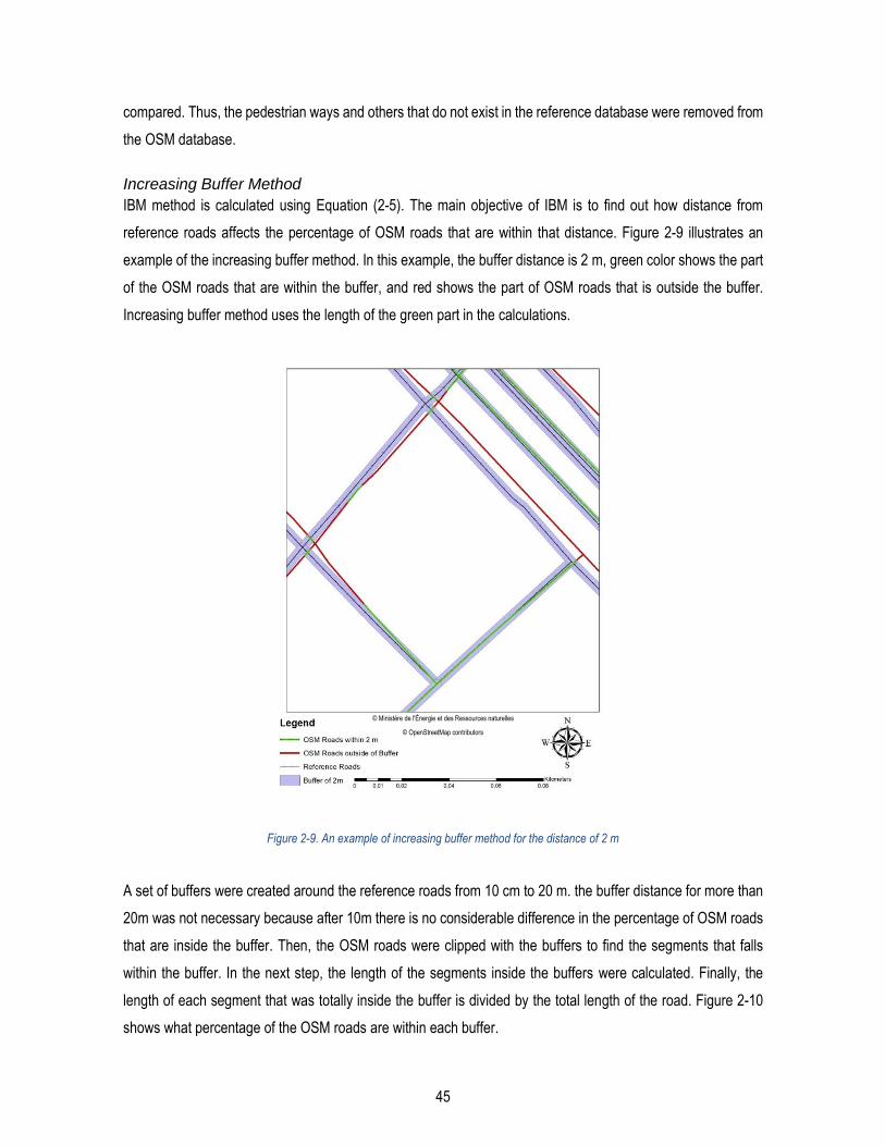
45
compared. Thus, the pedestrian ways and others that do not exist in the reference database were removed from
the OSM database.
Increasing Buffer Method
IBM method is calculated using Equation (2-5). The main objective of IBM is to find out how distance from
reference roads affects the percentage of OSM roads that are within that distance. Figure 2-9 illustrates an
example of the increasing buffer method. In this example, the buffer distance is 2 m, green color shows the part
of the OSM roads that are within the buffer, and red shows the part of OSM roads that is outside the buffer.
Increasing buffer method uses the length of the green part in the calculations.
Figure 2-9. An example of increasing buffer method for the distance of 2 m
A set of buffers were created around the reference roads from 10 cm to 20 m. the buffer distance for more than
20m was not necessary because after 10m there is no considerable difference in the percentage of OSM roads
that are inside the buffer. Then, the OSM roads were clipped with the buffers to find the segments that falls
within the buffer. In the next step, the length of the segments inside the buffers were calculated. Finally, the
length of each segment that was totally inside the buffer is divided by the total length of the road. Figure 2-10
shows what percentage of the OSM roads are within each buffer.
© OpenStreetMap contributors
© Ministère de l'Énergie et des Ressources naturelles

46
Figure 2-10. The positional accuracy of the OSM road network using increasing buffer method
Figure 2-10 illustrates that the changes in the percentage of OSM roads inside the buffer changes dramatically
when the buffer distance is between 0 and 5 m. For buffer distances greater than 5m there is a marginal change
in the percentage of OSM roads inside the buffer. When the buffer distance is greater than 8m, almost there is
no change. Hence, it can be concluded that the majority of OSM roads (almost 80%) are within the distance of
8 m from “Données Québec” roads. This positional accuracy can be considered sufficient for a wide range of
applications. However, each user should decide if this accuracy is enough for her/his specific application.
In order to better understand the positional accuracy of roads in the Québec province, we analyzed the positional
accuracy of each type of road in the OSM database using the increasing buffer method. Given that IBM does
not find corresponding features, it is assumed that each type of road is compared to the same type in the
reference database. Figure 2-11 illustrates the percentage of each type of road that is within 5 m of reference
roads. The buffer is created at the distance of 5 m because Figure 2-11 shows that 5 m is a turning point for
positional accuracy. Then, the calculations are done for each type of roads separately.

47
Figure 2-11. The positional accuracy of each type of road
Figure 2-11 shows that almost the majority of road types have an accuracy better than 60% except “unknown”,
“track_grade5”, “track_grade4”, “track_grade3” and “path”. Among these types, only “path” has a considerable
total length in the OSM database (7,999,418.99 m). In fact, the type of road is the values associated with the
key “highway”. There is a full list of available values for OSM road types on OpenStreetMap wiki webpage
(https://wiki.openstreetmap.org/wiki/Key:highway). Based on this webpage, “path” is any non-specific path that
can be located mainly outside of the cities and it can justify why the positional accuracy of “path” is not as good
as the other types. In addition, Figure 2-11 illustrates that “motorway”, “motorway_link”, “primary” and “trunk_link”
have the highest positional accuracy.
In the next step, in order to better evaluate the positional accuracy of the OSM road network, the positional
accuracy was calculated for each grid cell. Similar to the previous section, a grid of 1km*1km was used to
evaluate OSM positional accuracy. Then, IBM was applied for each grid and the result was unified to make a
map of the positional accuracy of the province.
0 10 20 30 40 50 60 70 80 90 100
living_street
motorway
motorway_link
path
primary
primary_link
residential
secondary
secondary_link
tertiary
tertiary_link
track_grade1
track_grade2
track_grade3
track_grade4
track_grade5
trunk
trunk_link
unclassified
unknown
Percentage of OSM roads within 5m buffer

48
Figure 2-12. Positional accuracy of OSM roads calculated using IBM with 1m, 2m and 5m buffers
Figure 2-12 illustrates the positional accuracy of OSM roads in the province of Québec. Three buffer distances
were used: 1m, 2m, and 5m. According to 1m buffer, most parts of the province have a low accuracy and almost
© Ministère de l'Énergie et des Ressources naturelles

49
there is no clear pattern in the accuracy. The accuracy results of 2m buffer shows that the parts that are close
to Montréal have a better accuracy than other parts. Finally, when 5m buffer is used, positional accuracy is
acceptable for the most part of the province. Moreover, it can be concluded that in lower buffer distances, there
is no pattern in the accuracy results but for greater buffer distances, better accuracy is obtained near the big
cities. Therefore, it can be concluded that errors in lower buffer distances do not follow a pattern. In order to
better evaluate this hypothesis, statistical methods should be applied. However, one possible explanation is that
the accuracy of the aerial imagery in OSM is ±4m, and digitizing the aerial imagery cannot have a better result
for low buffer distances.
Double buffer method
In this section, a double buffer method was applied to compare the results with the results of increasing buffer
method. The double buffer method is more robust in comparison to IBM because the double buffer method is
less affected by sudden changes. Figure 2-13 illustrates how the double buffer method works.
Figure 2-13. An example of double buffer method
© Ministère de l'Énergie et des Ressources naturelles

50
1 m buffer was created around both reference roads and OSM roads. Then, the intersection of these two buffers
was calculated. The green color illustrates the polygons that are created by intersecting the two buffers. The
area of the intersection is area 1 of DBM. According to DBM, the measure of positional accuracy can be
calculated as follows:
𝑃𝑜𝑠𝑖𝑡𝑖𝑜𝑛𝑎𝑙 𝐴𝑐𝑐𝑢𝑟𝑎𝑐𝑦 𝐷𝐵𝑀 =2∗𝐴𝑟𝑒𝑎1
𝐴𝑟𝑒𝑎(𝐵𝑢𝑓𝑓𝑒𝑟(𝐿1))+𝐴𝑟𝑒𝑎(𝐵𝑢𝑓𝑓𝑒𝑟(𝐿2))∗ 100 ( 2-10 )
If the two lines are exactly equal, then the area 1 will be equal to 𝐴𝑟𝑒𝑎(𝐵𝑢𝑓𝑓𝑒𝑟(𝐿1)) and
𝐴𝑟𝑒𝑎(𝐵𝑢𝑓𝑓𝑒𝑟(𝐿2)). Thus, the DBM will be 1. If the two lines are completely different, then the measure will
be 0 because area1 will be 0. Equation (2-10) is calculated for the province of Québec using 1m buffer around
both sets of roads. This result should be compared to the result of increasing buffer method when the buffer
distance is 2m because in DBM two buffers of 1m are used at the same time.
Figure 2-14. Positional accuracy of the OSM roads calculated by double buffer method using 1m buffers
© Ministère de l'Énergie et des Ressources naturelles

51
Figure 2-14 shows the positional accuracy of OSM roads that was evaluated using double buffer method. Buffers
of 1 m were created around OSM and reference roads. Then, the measure of positional accuracy of the double
buffer method was calculated. Finally, this measure was calculated for each grid. In addition, Figure 2-14
illustrates the positional accuracy of OSM roads around the city of Montreal.
Attribute Accuracy
As it is mentioned earlier, in this section only the name accuracy for the streets will be evaluated. Name is a
nominal variable and basically, it is a string. One of the methods that can efficiently compare two strings is
Levenshtein distance. Levenshtein distance is the minimum number of deletes, inserts, and substitutions that
are required to change one string to the other one. Therefore, it can be between 0 and the length of the longer
string. In this section, Levenshtein distance is calculated between the road name in OSM and its corresponding
name in the reference database. The accurate names of the roads will result in the accurate geocoding and is
necessary for many applications that work with addresses. The errors in road names are mainly due to typo
errors, unfamiliarity of the contributor with the environment, and more rarely to vandalism. Table 2-1 shows some
common errors that exist in the OSM database in Québec province.
Table 2-1. The frequent errors that exist in the road names in the province of Québec
id Name of Road in OSM Name in the Reference database Levenshtein Distance
1 Boulevard Joliet Boulevard Jolliet 1
2 Rue De La Verendrye Rue De La Vérendrye 1
3 Rue Néré Duplessis Rue Nérée-Duplessis 1
4 Rue De La noë Rue Delanoë 2
5 Rue Jacques-Cartier Route Jacques-Cartier 2
6 Chemin Gérard-Vigneau Chemin Gérard-Vigneault 2
7 Chemin St.Germain Chemin Saint-Germain 4
8 Rang du Pin-Rouge North Rang du Pin-Rouge Sud 5
9 Rue Gauthier Rue Jean-Gauthier 5

52
10 Rue J.-Albert-Daris Rue Joseph-Albert-Daris 5
The errors that we found in the road names are usually one of the following cases:
• Errors that are related to French accents.
• Typographic errors
• Errors that are related to the abbreviation of names
• Errors related to suffixes and prefixes like north and south
• Errors when the name is totally different
Usually, Levenshtein distances lower than 2 are related to typographic errors and French accents. The
Levenshtein distances greater than 5 are related to the cases that the name is totally wrong. Levenshtein
distances between 2 to 5 are related to suffixes and abbreviations.
Figure 2-15. Value of Levenshtein distance for the whole province of Québec
Figure 2-15 shows the attribute accuracy of Québec roads. Most of the names of the roads are correct in the
OSM database (87.6%). It means that the name of 87.6% of the roads was exactly the same in both databases
which is a good quality for many applications. 5.9% of the OSM roads’ names have 6 or more letters different
from the name in the reference database. In this research, we observed that more than 6 different letters means
that the road name is likely totally wrong in the OSM database. 4.2% of the roads’ names have 1 or 2 letters
different from the reference database. Our observations show that 1 or 2 letters difference is mostly because of
French accents or typo errors. Therefore, almost 4% of the names have issues related to French accents or typo
errors. The issue of French accent is especially important for the province of Québec and in other parts of
87
.6
3.2
1 0.8
0.7
0.4 5
.9
0 1 2 3 4 5 6 +
PERCENTAGE
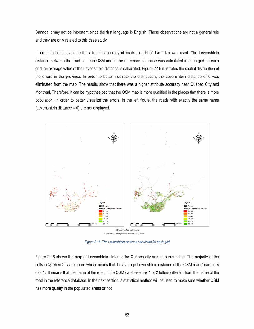
53
Canada it may not be important since the first language is English. These observations are not a general rule
and they are only related to this case study.
In order to better evaluate the attribute accuracy of roads, a grid of 1km*1km was used. The Levenshtein
distance between the road name in OSM and in the reference database was calculated in each grid. In each
grid, an average value of the Levenshtein distance is calculated. Figure 2-16 illustrates the spatial distribution of
the errors in the province. In order to better illustrate the distribution, the Levenshtein distance of 0 was
eliminated from the map. The results show that there was a higher attribute accuracy near Québec City and
Montreal. Therefore, it can be hypothesized that the OSM map is more qualified in the places that there is more
population. In order to better visualize the errors, in the left figure, the roads with exactly the same name
(Levenshtein distance = 0) are not displayed.
Figure 2-16. The Levenshtein distance calculated for each grid
Figure 2-16 shows the map of Levenshtein distance for Québec city and its surrounding. The majority of the
cells in Québec City are green which means that the average Levenshtein distance of the OSM roads’ names is
0 or 1. It means that the name of the road in the OSM database has 1 or 2 letters different from the name of the
road in the reference database. In the next section, a statistical method will be used to make sure whether OSM
has more quality in the populated areas or not.
© Ministère de l'Énergie et des Ressources naturelles
© OpenStreetMap contributors

54
Figure 2-17. Levenshtein distance for each grid around Québec city
Statistical Analysis
As discussed in section 2.4, if a variable has a significant correlation with a quality measure, then that variable
can be used as an indicator for that quality measure. The quality indicators can provide an insight into the quality
measures when it is not possible to calculate quality measures directly. In this section, statistical analysis is
applied to determine if there is a correlation between the three quality measures and the five variables including
the population in each region, the average income in each region, the density of OSM buildings in each region,
the density of OSM roads in each region, and the number of POIs in each region. Due to limited access to current
data, only these five variables are selected and evaluated in this research. These five variables are extracted
from the literature review. Each of these five variables are mentioned at least in one of the previous researches
(see section 2.4). However, to our best knowledge, no research carried out a complete analysis to evaluate the
correlation between these variables and the three quality measures (completeness, positional accuracy, and
attribute accuracy). For example, [10] proved that there is a positive correlation between completeness and the
density of OSM data, but, to our best knowledge, no research evaluated the correlation between the density of

55
OSM data and positional accuracy or attribute accuracy. Thus, in this research, a complete statistical analysis
is done to find out which variable can be used as an indicator for which quality measure. In addition, the result
of this section determines which variable has the strongest and which one has the weakest correlation with each
quality measure.
Calculating the correlation between quality measures and quality indicators
The correlation coefficient is a statistical measure that shows how the change of one variable can affect the
other one. For example, it can tell us whether the completeness of OSM database increases in the areas where
there is more population. Pearson correlation coefficient can detect a linear relationship between two variables.
However, nonlinear relations are not detected by Pearson. Spearman’s rank correlation coefficient can detect
all kind of monotonic relationships. Monotonic relationship is more general than linear relation and includes all
relations where the increase of one variable increases the other one. Hence, here in this paper, Spearman’s
rank correlation coefficient is used to calculate the correlation between the five variables and quality measures.
To achieve this goal, the study area is intersected with a grid of 1km*1km. Then, the five variables and the three
quality measures are calculated for each grid cell. Each grid cell is considered as a data sample for calculating
the Spearman’s rank correlation coefficient.
Table 2-2. Correlation coefficient between quality measures and potential quality indicators
Category Potential Quality Indicators Complet. Positional Accuracy Attribute
Accuracy
Variables
Pop
ulat
ion
Inco
me
OS
M R
oads
Den
sity
OS
M B
uild
ings
Den
sity
Num
ber
of P
OIs
Com
plet
enes
s
IBM
1m
IBM
5m
DB
M 2
m
Leve
nsht
ein
Dis
tanc
e
Population 1 0.684 0.480 0.306 0.222 0.509 0.222 0.321 0.306 -0.109
Income * 1 0.427 0.265 0.192 0.455 0.200 0.256 0.281 -0.102
OSM Roads
Den.
* * 1 0.324 0.254 0.950 0.157 0.044 0.133 0.009
OSM Buil. Den. * * * 1 0.432 0.301 0.104 0.160 0.128 -0.007

56
Number of POIs * * * * 1 0.215 0.076 0.094 0.088 0.048
Completeness * * * * * 1 0.053 0.011 0.021 -0.261
IBM 1m * * * * * * 1 0.700 0.696 -0.189
IBM 5m * * * * * * * 1 0.739 -0.170
DBM 2m * * * * * * * * 1 -0.199
Levenshtein
Dist.
* * * * * * * * * 1
Table 2-2 shows the correlation between the five variables and quality measures. The five variables are:
population, income, density of roads, density of buildings and number of POIs in each grid. The quality measures
are: completeness, positional accuracy (increasing buffer method IBM at buffer distance of 1m and 5m),
positional accuracy calculated by double buffer method at the buffer of 2 m and attribute accuracy (comparing
the names of the streets using Levenshtein distance). In addition, this table shows the correlation between
quality measures. It helps us to understand whether a quality measure can be used as an indicator for the other
quality measures.
The results show that completeness has a positive correlation with all 5 variables. Completeness has the
strongest correlation with the density of OSM roads in each grid (0.95) which means that the density of OSM
roads is a very powerful indicator of completeness. The next powerful correlations exist between completeness
and population and income (almost 50%). The results demonstrate that the completeness of OSM roads
increases with the increase of the number of POIs, but the correlation is not as strong as the one of previous
indicators.
In the case of positional accuracy, the correlation is positive, but it is not as strong as completeness. In addition,
IBM 5 m has a stronger correlation with quality indicators than IBM 1 m. One possible explanation is that the
areal images are not considered to have a quality better than 4 m. Thus, when the buffer of 1 m is selected, the
behavior of positional accuracy is more random than when the buffer of 5 m is selected. Moreover, positional
accuracy has the strongest correlation with population and income.
Statistical hypothesis testing
The correlation between quality measures and quality indicators is calculated in the previous section. However,
these correlation values are not sufficient to accept or reject a positive association (relationship) between the

57
quality measures and quality indicators. In this research, statistical hypothesis testing is used to determine
whether a significant positive association exists between the quality measures and quality indicators. The H0
and H1 hypotheses are as follows:
• H0: There is no significant positive association between the quality measures and quality indicators
(variables of Table 2-2).
• H1: There is a significant positive association between the quality measures and the quality indicators.
This test is a one-tail test and the number of pairs is 363,111 (which is the number of grid cells in all cities).
Therefore, the critical value of Spearman’s correlation test is ρc = 0.003 at the significance level of 0.05. It meas
that any correlation greater than 0.003 rejects the null hypothesis and proves a positive association between the
two variables. Table 2-3 shows the results of statistical test for the variables of Table 2-2. The letter Y means
that a positive association is accepted, while letter N means that the positive association is not accepted.
Table 2-3. Result of Spearman’s correlation test between the quality measures and quality indicators
Category Potential Quality Indicators Complet. Positional Accuracy Attribute
Accuracy
Variables
Pop
ulat
ion
Inco
me
OS
M R
oads
Den
sity
OS
M B
uild
ings
Den
sity
Num
ber
of P
OIs
Com
plet
enes
s
IBM
1m
IBM
5m
DB
M 2
m
Leve
nsht
ein
Dis
tanc
e
Population Y Y Y Y Y Y Y Y Y Y
Income * Y Y Y Y Y Y Y Y Y
OSM Roads
Den.
* * Y Y Y Y Y Y Y N
OSM Buil. Den. * * * Y Y Y Y Y Y Y
Number of POIs * * * * Y Y Y Y Y N
Completeness * * * * * Y Y Y Y Y
IBM 1m * * * * * * Y Y Y Y

58
IBM 5m * * * * * * * Y Y Y
DBM 2m * * * * * * * * Y Y
Levenshtein
Dist.
* * * * * * * * * Y
Table 2-3 shows that a positive association at the significance level of 0.05 is proved between all pairs of
variables except 2 of them. The test rejected the positive association between the attribute accuracy of OSM
roads and the density of OSM roads in our study area. In addition, the test rejected the positive association
between the attribute accuracy of OSM roads and the density of POIs in each grid cell in our study area. The
value of Levenshtein Distance increases by the decrease of attribute accuracy and vice versa. Thus, the test for
attribute accuracy is a left-tailed test.
Statistical hypothesis testing allows evaluating the significance of a correlation in a statistical analysis.
In the case of attribute accuracy, high values of Levenshtein distance indicate lower accuracy and in the contrary,
low values of Levenshtein distance indicate high attribute accuracy. Therefore, a negative correlation between
Levenshtein distance and quality indicators shows a positive correlation between attribute accuracy and the
indicators. The results demonstrate that Levenshtein distance does not have any strong correlation. The
strongest correlation is between Levenshtein distance and completeness (-0.26) which means that where the
map is more complete, attribute accuracy is higher. The values of correlation for Levenshtein distance are
generally negative which means that there is a weak positive correlation between attribute accuracy and quality
indicators.
Conclusion
The results of this research show that the OSM road network is 32.91% complete in the province of Québec. In
urban areas, OSM is even more complete than the reference database because OSM contains pedestrian roads.
Thus, OSM is almost complete in urban areas.
The results of positional accuracy evaluation show that the percentage of roads that fall in the vicinity of the
reference roads increases dramatically when the buffer size increases to 5m and then it grows gradually till the
buffer size of 8m and after 8m there is no considerable change in the positional accuracy. Approximately, 70%
of the roads of the province has a positional accuracy better than 5m. In addition, there is no noticeable difference
between the positional accuracy of the different types of roads. Thus, in the province of Québec, the type of the

59
road is not an indicator of the positional accuracy. When 5m or greater buffers are used, the roads near cities
have a better positional accuracy, while with the buffers smaller than 5m there is no pattern in the accuracy.
Attribute accuracy shows that the name of 87.6% of the OSM roads is exactly the same as their name in the
reference database. 3.2% of the roads have only 1 letter different and 1% of the roads have two letters different
from the name in the reference database. One of the most frequent errors of attribute accuracy is related to the
French accent. Suffixes and prefixes are also a serious problem. For 5.9% of the roads, there are 6 or more
different letters in the name.
The statistical analysis shows that population, income, and OSM road density have a positive correlation with
quality measures. It means that they can be used as quality indicators for the areas where there is no information
about the quality of OSM. Among the three quality indicators, the population has the strongest correlation with
quality measures. The correlation between quality indicators and completeness is greater than the correlation
between quality indicators and attribute accuracy. It means that they are stronger indicators for completeness
than for attribute accuracy.

60
Evaluating the Quality of OSM
Buildings
Introduction
The term VGI was introduced by Goodchild to describe the process of geographic data production by general
public [3]. This term also refers to the fact that VGI data are acquired voluntarily by the crowds of people. VGI
can cover a wide range of data including personal trajectories, geotagged photos, and the voluntarily digitized
elements of online maps [25]. VGI can be categorized into three groups based on the data content including
text-based VGI, image-based VGI, and map-based VGI [22]. Text-based VGI can be a georeferenced tweet,
while image-based can be a geotagged photo. A map-based VGI can be created by online communities where
the contributors can edit, create, and delete the features on a web map. In fact, map-based VGI is a
geographically-explicit kind of VGI where the contributors explicitly contribute to the production of geographic
contents [5].
A good example of a web-based VGI is OpenStreetMap. OpenStreetMap was created by Steve Coast and is a
free, open editable map of the world [45]. OSM allows contributors to edit, create, and delete the content of the
map of the world. A number of researches reveal the fact that the majority of the contributions to OSM are not
uniform. This implies that there are places with huge contributions whereas other places have very few
contributions [6], [98]. OSM contributors have already created a nearly complete map of the world in many parts
such as Europe and North America [5], [23]. OSM contributors mainly digitize roads, buildings, and land use
data. The contributors can edit the map in their own neighborhood or in any other area of the map. For instance,
when the Haiti Earthquake happened in 2010, the contributors of OSM tried to digitize a map of Haiti which
helped NGOs to provide their help for the local people [52].
The availability of the almost freely accessible OSM data can encourage the development of many applications
that were not possible before due to the lack of access to geographical data [85]. The license of OSM allows
sharing, using, and reproduction of the data even for commercial purposes as far as the contributors of OSM
are credited [48]. The data of OSM is downloadable from http://www.geofabrik.de/. This website provides the
data for different countries of the world. In addition, the full history of the OSM database is available and it allows
the researchers to track all changes to the database [99].
The geographic data in OSM can be stored in three different forms including nodes, ways, and relations [5], [45].
The nodes represent point features, while ways represent the linear objects. The attribute data in OSM are
stored as tags. OSM allows the contributors to use tags to describe features which is both a strength and a
weakness of the project. Tags are in the form of “key=value” pairs [5], [45]. For instance, a building can be stored

61
using a “building=yes” tag. The name of the building can be stored in the form of “name=Casault”. A number of
tags are widely accepted by the community and there is a consensus about them, while some other tags are
chosen by a contributor and are not accepted by others.
For OSM, the majority of contributions done by only a few of the contributors. A rule of thumb explains that only
1% of the contributors produce the majority of the data and 9% of them contribute on a regular basis, while 90%
of the contributors of OSM just contribute once or a few times and then withdraw from the project [48]. There is
no requirement for becoming a contributor to the project. In addition, many of the contributors do not have any
geographic knowledge and are not necessarily familiar with spatial data collection rules and procedures [10].
Therefore, there is no guarantee about the quality of OSM data and hence, it is necessary to assess the quality
of the data before using it in any application.
A variety of researches have been done in order to evaluate the quality of OSM data in different regions of the
world [10], [46], [59], [68], [81], [85]. One of the first evaluations of the quality of OSM buildings is done by [68].
They used a turning function approach to measure the shape accuracy. Another research [67] evaluated how
the quality of OSM database changes over time. [4] proposed a new method based on coordinate transformation
for finding the equivalent edges and vertices of features in OSM and a reference database. [23] evaluated the
quality of OSM building footprints data in the city of Ottawa. Another research evaluated the quality of OSM
building data in Taiwan [100]. Some researchers tried to find out the relation between the quality of the OSM
building data and indicators such as the density of the building [10].
Considering the fact that the primary goal of OSM is to provide spatial data for the regions where the authoritative
data is not available, comparison to reference data in those regions is not possible [10]. To overcome this
problem, a number of researchers suggested the use of quality indicators such as population, the number of
contributors, and the average income of the region as indicators to describe the quality of OSM in those regions.
In this chapter, first of all, research is done to find out different quality measures that previous research works
have used to evaluate the quality of OSM bulidings. Then these quality measures are classified for estimating
different aspects of quality such as completeness and positional accuracy. Then, the quality of OSM buildings
for 5 cities (Québec City, Longueuil, Repentigny, Rouyn-Noranda, and Shawinigan) in the province of Québec
is evaluated. In the last step, each measure of the quality is calculated for each grid of 1km*1km and then the
correlation between the potential quality indicators and the quality measures are calculated. This step helps us
to understand whether or not the measures of quality decrease or increase by these indicators.

62
Methodology
Feature Matching
Feature matching is a process that aims to find corresponding features between multiple databases [68]. In this
method, first a level of tolerance is defined and then the similarity and dissimilarity between two features are
measured. Then, based on the defined tolerance level, the two features are identified as corresponding or
independent. Given that a geographic feature can be described by its geometry and a set of attributes, the
similarity measures can be based on a comparison of lexical information, position of the feature, shape of the
feature, or even attributes that describe the feature. Feature matching is considered as an essential step in data
integration, data update, change detection, and data versioning [101].
Feature matching in OpenStreetMap is even more difficult than feature matching in authoritative databases
because OSM data is heterogonous and there may be a high density of data in one neighborhood and a very
low density in others. In addition, different OSM features do not have the same level of details [22]. It is because
OSM does not force the contributors to use a unique way of data creation [53]. For example, contributors may
digitize a very complex building footprint with only 4 points. In fact, usually, the building footprints in OSM are
generalized in comparison to the real footprint [67]. Therefore, the buildings of an authoritative database may
follow the same level of detail but in the case of OSM, the same level of detail cannot be expected due to polygon
generalization. Overall, a comparison of attributes (tags) or geometry between an OSM feature and a reference
feature is far more complicated than comparing two authoritative databases.
A number of researchers proposed models for feature matching in OpenStreetMap. [52] proposed a method for
matching the OSM road network with a reference road network. The method can automatically find
corresponding roads using a seven-step comparison algorithm [52]. The method computes geometrical and
topological information of a line (such as distance and direction) as well as attributes of the line such as the
name of the street [52]. However, [101] believes that this method is not very efficient because of the existence
of topological inconsistencies in the OSM database.
Another feature matching method is proposed by [101]. This method uses a level of tolerance which is a buffer
around the geometry and then the location of the second geometry in comparison to this buffer is evaluated.
The second geometry can be within, partly within or completely outside of the buffer. The width of the buffer is
considered as the maximum acceptable difference between the two geometries. The method also measures the
similarity between lexical information of the two features. Usually, lexical information is stored in strings and this
step of the algorithm actually compares two strings [101]. Even though this algorithm had an acceptable result
in some regions, it seems to be computationally heavy. In addition, most of the buildings do not have a name.
63
Thus, comparing them by their names of other tags is not as efficient in buildings as it is in the case of road
network matching.
Previous researches on OSM building quality mainly applied two methods for matching building footprints of
OSM with a reference database. The first method, which is more common, is the area overlapping method
introduced by [68]. This method is based on assumption that the polygon displacement between OSM and the
reference database is not considerable [68]. Therefore, the area that the two polygons overlap can be used as
a criterion for finding corresponding features [68]. The tolerance for feature matching is considered 30% of the
area [68]. If the overlap area between the OSM and reference feature is less than 30%, the two features will not
be considered corresponding because it is assumed that the overlap is caused by the spatial displacement of
neighboring polygons. Then, if any two features in OSM and reference data has an overlap of more than 30%,
they will be considered as corresponding features [68]. The following equation was proposed by [68] for finding
corresponding building footprints:
𝐴𝑟𝑒𝑎𝑜𝑣𝑒𝑟𝑙𝑎𝑝
𝑀𝑖𝑛(𝐴𝑟𝑒𝑎(𝐹𝑜𝑜𝑡𝑜𝑠𝑚_𝑖),𝐴𝑟𝑒𝑎(𝑓𝑜𝑜𝑡𝑟𝑒𝑓_𝑗))> 30% ( 3-1 )
Most researchers who evaluated the quality of OSM building footprint data used this method [23], [73], [100],
[102]. The tolerance of 30% is not a fixed value and some of the other researchers considered other values as
tolerance. For example, [23] used a tolerance of 50% for the feature matching.
[67] proposed another method for feature matching, for calculation of completeness, which uses the centroid of
the OSM polygons and compare them to the reference database. If the centroid of an OSM building footprint
falls within a building footprint of the reference database, then the two polygons are corresponding [67]. [67]
applied this method to evaluate object-based completeness of the OSM building footprints. A number of
researchers applied centroid method for feature matching [23], [25], [51], [100] .
Another method of feature matching was proposed by [79]. This method first calculates the centroid of the two
datasets. Then, calculate the distance between the two sets of points. The nearest polygons will be considered
as matching polygons. A tolerance of 20m is used in this method and only OSM polygons that their nearest
reference polygon is nearer than 20m, are considered as a corresponding pair [79]. This method seems to be
the simplest among the proposed methods. However, no research has been found to compare the quality of all
these feature matching methods.

64
Correspondence types
The relationship between OSM features and reference features can be complicated. In particular, the relation
between the building footprints is more complicated due to the errors that may happen during the data creating.
For example, a block of 5 buildings can be represented by only one building on OSM because, in the aerial
imagery, it is difficult to determine the exact border between the roofs. The other problem is that usually, the
OSM polygon represents the roofs, not the footprints. Thus, it may have some displacements because the sensor
may have an oblique view of the buildings [103]. Therefore, the OSM buildings may be a combination of
reference buildings, a generalized representation of reference buildings, or a representation with a positional
displacement or a combination of all of these issues. [68] argued that the relationship between OSM footprints
and the footprints in the reference databases can be one of the following cases.
(OSM : reference):
• 1 : 1 – this relation exists when one OSM building is matched to only one reference building and that
reference building also matches to only one OSM building. From the data quality point of view, this
case is the only case where both datasets are complete.
• 1 : 0 – this case is when there is a building on OSM that has no corresponding polygon in the reference
database. Based on ISO standard, this case is called data commission [7].
• 1 : n – this case is when 1 OSM database is corresponding to more than 1 building in the reference
database. This case is frequent in OSM because the border between the roof of adjacent buildings is
not clear in aerial imagery and sometimes a block of buildings is represented by one polygon in OSM
[101].
• 0 : 1 – this case happens when a building in the reference database has no matching polygon in the
OSM database. ISO standard called it data omission [7].
• n : 1 – this case means that more than one building in the OSM database are matching with only one
building in the reference database. This case is also frequent in OSM because the difference in the
elevation of the different parts of a single building may cause the digitizers to consider it as a number
of separated buildings.
• n : m – this case means that a number of buildings in OSM are matching to a number of buildings in
the reference database. Based on our case study this case is more common with very big buildings
than with small residential ones.

65
Figure 3-1 illustrates some issues regarding OSM feature matching. In this figure, all polygons 1, 2, …, 6 are
moved towards the northwest in comparison to the reference polygons. Polygon 1 is smaller than the
corresponding reference polygon. It is also a generalized representation of the reference polygon. The fact that
OSM features are a generalized (simplified) representation of the reference ones is mentioned by [68]. Polygons
3, 4, 5, and 6 are corresponding to only one polygon in the reference database. This issue can be caused by
the poor aerial images or the difference in the elevation of different parts of the roof of one building that can
make it look like some separated buildings. Therefore, there are issues such as spatial displacement and
incorrect representations of reference building footprints. In addition, polygon 2 has an intersection with more
than 1 reference polygon, which may cause problems of feature matching if the method of polygon overlay is
used for feature matching.
Figure 3-1. The issues regarding matching OSM building footprints with reference ones
The issues that exist in the OSM polygon database, can cause errors in the previously mentioned feature
matching algorithms such as polygon- overlay and centroid checking. Figure 3-2 illustrates that polygon 2 has a
© OpenStreetMap contributors

66
considerable intersection with the wrong reference polygon. Furthermore, its centroid is located within the wrong
polygon. Therefore, both polygon overlay and centroid checking methods may fail in finding the corresponding
reference polygon for the polygon number 1. Both of these methods somehow compare the position of the
polygons in the two databases. I believe that comparing only the position of the polygons is not sufficient because
the spatial displacement of the OSM polygons in comparison to reference ones can cause errors in feature
matching. Thus, the author propose to not only compare the position of the two polygons but also compare their
shapes so that a more reliable matching can be achieved.
The second error can be the case of 3 to 7 which are represented by 5 different polygons in OSM but in the
reference database, they correspond to only one polygon. The centroid of all of these polygons are located
outside of the corresponding reference polygon. Therefore, the centroid method may fail to find the matching
polygons. However, if the union of these shapes is compared to the reference shape, then an acceptable level
of shape similarity exists between them. Hence, I believe that an algorithm that wants to find the correct matches
should compare not only the polygons individually, but it also should compare the union of all candidate polygons
to find out if the union has more similarity or not.
Figure 3-2. The errors of matching OSM building footprints with reference ones
© OpenStreetMap contributors

67
In order to overcome the previously mentioned problems in feature matching and have a more reliable method,
the I propose to add a shape comparison to the previous methods. In addition, the comparison and feature
matching should be done for all the possible subsets of the set of candidate polygons. In the next section, the
algorithm developed for this purpose is discussed.
Proposed algorithm
As mentioned in the previous section, there are a number of issues regarding feature matching for OSM
buildings. Due to the displacement, the centroids of OSM polygons may not necessarily fall within the correct
reference polygon. The positional accuracy of OSM polygons is relatively acceptable and for the majority of the
cases, the centroid falls within the correct object. However, there are still few cases where the centroids are not
within the corresponding polygon due to the poor spatial accuracy (displacement of the polygons). Moreover,
the displacement can cause an overlap between the target OSM polygons and a number of incorrect reference
features. To tackle thies issues, the authors propose a method that matches the features based on the
comparison of both position and shape of the polygons. Therefore, the results will be more reliable than
comparing only the position of the polygons or their centroids.
In addition, the other problem is that sometimes the difference in the elevation of different parts of a roof may
cause errors in digitizing the roof in the aerial images. [101] found that a number of OSM buildings are in fact a
block of buildings in reality but the borders between them are not clearly visible in the aerial images and they
are digitized as one polygon. Therefore, it is possible that a group of polygons in OSM correspond to only one
polygon in the reference database or vice versa. In order to tackle this issue, the authors proposed an algorithm
that first finds the candidate polygons and then check if any group of these candidates can be corresponding to
a polygon in the reference database.
The flowchart of the algorithm is explained in Figure 3-3. This algorithm has two inputs: the OSM polygons and
the reference polygons. Then, for each polygon in OSM, all the candidate reference polygons are identified using
a polygon overlay method (calculating the intersection between the OSM polygon and all reference polygons
withing that location). The candidate polygons are those that have more than int_tol% intersection with the OSM
polygon. The set of the candidate reference polygons is called T. Then, based on the cardinality of the set, 3
possible feature matching cases can happen. If |𝑇| = 0, then there are no candidate polygons in the reference
database and it means that the OSM polygon has no match in the reference database and it is a commission. If
|𝑇| = 1, then it means that the feature has only one matching polygon in the reference database which indicates
a good matching. If |𝑇| > 1, then there is more than one candidate for the OSM polygon. In this case, further
investigation is required to find out the correct matching polygons. Therefore, a shape similarity evaluation is

68
done between the OSM polygon and all possible subsets of T. Since it is not possible to compare the shape of
one polygon with two separate polygons, a concave hull is calculated for each subset of T. Then, the shape of
the OSM polygon is compared to the shape of the concave hull. If the concave hull of any subset of T has a
shape similarity to the OSM polygon greater than shp_tol% , then, the members of that subset of T will be
considered as the corresponding polygons of the OSM polygon and the relation will be 1 : n.
Figure 3-3. Polygon aggregation for feature matching
Figure 3-3 illustrates a number of examples when the aggregation of a group of polygons is matched with one
single polygon. The aggregated polygon may not be exactly similar to the reference polygon but if the similarity
is greater than shp_tol%, they will be considered as matching features.
The main steps of the proposed algorithm are:
1. Firstly, find all candidates by comparing their location to the location of the OSM polygon.
2. Secondly, find which group of candidates has a shape that better fits the OSM polygon.

69
Checking Shape Similarity
Checking the Overlap
Reference Polygons
Correspondence Type
Corresponding Polygons
OSM Polygons
Proposed Feature Matching Algorithm
Find all the subsets of TPset = Powerset(T)
ITI > 1
ITI = 1
ITI = 0
1:11:n1:0
YesNo
Select the first geometry from OSM: pi
Calculate Shape_Simil(pi, cj)
∀cj∈C
Output Psetj
where: Shape_Simil(pi, cj) is max
Output the qj where:
Intersection(qj , pi ) is max
Calculate
Intersection(pi, qj) ∀qj∈Q
C = {c1 , c2 , … , cn}
Pset = {Pset1, Pset2, …
, Psetn}
FindT = {qj | intersection (qj ,
pi ) > int_tol%}
Calculate
ITI
Shape_Simil(pi, cj)> shp_tol% ?
Q = {q1, q2, … , qn}
P = {p1, p2, … , pn}
T = {q1, q2, … , qn}
CalculateC = {cj |cj = Concave Hull
(Psetj)} ∀Psetj∈Pset
Figure 3-4. Proposed feature matching algorithm

70
When the relationship between OSM and reference database is evaluated, then, the relation between reference
database and OSM should be evaluated using the same algorithm and just by changing the inputs. This reverse
relation evaluation facilitates the discovery of the other types of relations that are not in the flowchart of Figure
3-4.
Completeness
Completeness refers to whether or not objects in the real world and their attributes exist in the database [36].
Usually, completeness has two main components: data completeness and model completeness [36]. In this
study, only data completeness for building footprints is evaluated. Attribute completeness expresses how
completely the attributes that describe the characteristics of a feature exist in the database [36]. Two main issues
are related to completeness evaluation of the data: commission and omission [7]. Commission is when the
object in the database does not exist in the real world and omission happens when an object in the real world is
not mapped in the database [7]. In the case of building footprints of the OSM database, completeness means
how complete the buildings of the study area are mapped by the OSM contributors.
There are two common methods for evaluating the completeness of OSM building footprints: unit-based method
and object-based method [67]. The unit-based method compares the total area of the building polygons of the
OSM database to the total area of the building footprints of the reference database in the study area [67]. The
object-based method compares the total number of the OSM buildings in an area to the total number of buildings
in the reference database in that area [67]. The unit-based method is easier because it does not require feature
matching and it just compares the total area of the polygons of the two databases. However, the object-based
method requires finding the corresponding features before comparing numbers. [67] compared the two methods
and suggested the use of an object-based method because the unit-based method is highly sensitive to
disparities between the building footprints in OSM and building footprints in the reference databases. [69]
compared the two methods of completeness evaluation and found that neither of them pay attention to the
geometrical representation of the buildings. Therefore, both methods have shortcomings that may result in
overestimation or underestimation of the completeness [69]. For example, when a block of buildings in the real
world are represented with just one polygon in OSM, comparing the total number of buildings may underestimate
the completeness [69]. [69] proposed to merge the adjoining buildings in both databases and then compare the
resulting polygons and calculate three parameters: true positive, false negative and false positive. This method
tries to solve the problem that sometimes, adjoining buildings are represented by only one polygon. However, I
prefer to use an object-based method with a precise feature matching because this method does not change
the input polygons by merging them, thus, its results are more tangible. The authors believe that a precise feature
matching can discover the relationship between OSM and reference database. Hence, the problem of 1 : n or n
: 1 matching can be handled.

71
Unit-based method
In the unit-based method, the completeness is simply calculated based on the ratio of the total area of buildings
in OSM to the total area of buildings in the reference database [23]. This method is not computationally heavy.
However, a number of issues can cause uncertainty in the results [69]. Unit-based completeness can be
calculated using the following equation [67]:
𝐶𝐴𝑟𝑒𝑎 =∑ 𝐴𝑟𝑒𝑎(𝑓𝑜𝑜𝑡𝑝𝑟𝑖𝑛𝑡𝑂𝑆𝑀)𝑛
𝑖=1
∑ 𝐴𝑟𝑒𝑎(𝑓𝑜𝑜𝑡𝑝𝑟𝑖𝑛𝑡𝑅𝑒𝑓𝑒𝑟𝑒𝑛𝑐𝑒)𝑚𝑗=1
( 3-2 )
where n is the number of buildings in OSM and m is the number of buildings in the reference database. A number
of researches applied the unit-based method for assessing the completeness of OSM building footprints [23],
[51], [67], [68].
Object-based method
In an object-based method, first, the corresponding features are detected. Then, the completeness is calculated
based on the comparison of the ratio between the number of the features or the area of the features in OSM and
their number or area in the reference database. Therefore, it is more reliable for completeness assessment [67].
The object-based completeness evaluation of OSM buildings using the centroid method, can be done using the
following equation [67]:
𝐶𝑐𝑒𝑛𝑡𝑟𝑜𝑖𝑑 = ∑ 𝐶𝑒𝑛𝑡𝑟𝑜𝑖𝑑𝑟𝑒𝑓_𝑖𝑛_𝑂𝑆𝑀
∑ 𝐶𝑒𝑛𝑡𝑟𝑜𝑖𝑑𝑟𝑒𝑓× 100 ( 3-3 )
In fact, this equation is the same as the unit-based method except it applies only to the matching polygons. The
object-based completeness evaluation based on polygon-overlap method can be done using the following
equation [67], [68]:
𝐶𝑜𝑣𝑒𝑟𝑙𝑎𝑝 = ∑ 𝐵𝑢𝑖𝑙𝑑𝑖𝑛𝑔𝑠𝑟𝑒𝑓_𝑜𝑣𝑒𝑟𝑙𝑎𝑝_𝑂𝑆𝑀
𝐵𝑢𝑖𝑙𝑑𝑖𝑛𝑔𝑠𝑟𝑒𝑓× 100 ( 3-4 )
The difference between these two equations is the way they find corresponding features. Any other method for
feature matching can be used instead of the centroid or overlapping methods. Then, the completeness can be
evaluated by calculating the proportion of the matched buildings in OSM to those of the reference database. The
proportion can be calculated by comparing the number of matched buildings or their area. In this research, first,
the two databases are matched. Then, the two completeness values are calculated. The first one calculates the
ratio of the number of matched OSM features to those of the reference database, while the second method
calculates the ratio of the area of the OSM features to the area of the matched reference features. The
comparison of the two methods can provide an insight into the completeness of the OSM database.

72
Positional accuracy
In GIS, the position of an object in the real world is expressed in an spatial coordinate system and is stored in
the databases [36]. The position of the objects of the real world can be obtained by repeated measurements
[36]. The precision of the position refers to the spread of the results obtained by the measurements [36].
However, accuracy is the distance from the measured position to the true position (which is unknown) [36]. The
ISO standard for spatial data quality defines positional accuracy as the accuracy of the position of objects with
respect to a coordinate system [7]. Positional accuracy has three elements: absolute accuracy, relative
accuracy, and gridded data positional accuracy [7]. Absolute accuracy is the closeness of the measured
coordinates in comparison to the true coordinates, while the relative positional accuracy refers to the positional
accuracy of the objects of the map with respect to the position of the other objects [7].
A number of researches evaluated the positional accuracy of the OSM building footprints [25], [68]. The common
point among all these researches is that they mostly used a reference database to compare with OSM. [68]
evaluated the positional accuracy of building footprints of OSM by comparing the position of their corresponding
vertices. Firstly, this method finds the corresponding vertices of the OSM polygon and the reference polygon.
Then, it calculates the average distance of these points as a measure of the positional accuracy of the buildings
[68]. Only the buildings with a 1 : 1 relation are included in the calculations. Finally, they calculated 4 measures
including maximum offset, minimum offset, average offset and standard deviation [68].
[4] proposed a method for evaluating the positional accuracy of the OSM building footprints. In the first step,
this method estimates the parameters of an affine transformation between OSM building vertices and
corresponding reference vertices [4]. A manual detection of more than 4 homologous points are required for
each region of the map [4]. Finally, all the points of OSM are transformed using the affine transformation. Then,
they are compared to the corresponding points of the reference database [4]. The distance between the two
homologous points is the measure of positional accuracy in this method [4].
A simple but efficient method of positional accuracy assessment for building footprints of OSM is applied by [25].
[25] compared the position of the centroid of the building on OSM to the centroid of the corresponding building
in the reference database. The distance between the two centroids can be used as an indicator for the positional
accuracy [25]. The measure of positional accuracy of this method is calculated as:
𝐷𝑖𝑠𝑡𝑎𝑛𝑐𝑒𝑎𝑣𝑒𝑟𝑎𝑔𝑒 = ∑ √(𝑋𝑂𝑆𝑀𝑖 − 𝑋𝑟𝑒𝑓
𝑐𝑜𝑟𝑟𝑒𝑠𝑝𝑜𝑛𝑑𝑖𝑛𝑔)
2+ (𝑌𝑜𝑠𝑚
𝑖 − 𝑌𝑟𝑒𝑓𝑐𝑜𝑟𝑟𝑒𝑠𝑝𝑜𝑛𝑑𝑖𝑛𝑔
)2
𝑛𝑖=1 ( 3-5 )

73
where 𝑋𝑟𝑒𝑓𝑐𝑜𝑟𝑟𝑒𝑠𝑝𝑜𝑛𝑑𝑖𝑛𝑔
is the X coordinate of the centroid of the polygon in the reference database that is
corresponding to the centroid of the ith polygon of OSM and n is the number of OSM buildings that have a 1 : 1
relationship with reference buildings.
The distance is not the only parameter that can be measured between the two centroids. [84] proposed an
intrinsic quality indicator that compares the displacement of the road junctions over the time. In a normal case,
the displacement of the road junctions should be distributed uniformly in all directions [84]. However, vandalism
can affect distribution in one direction more than others [84]. The authors believe that this method can be used
for building centroids. Therefore, we propose not only to compare the distance between the two centroids but
also to evaluate the distribution of the directions. The evaluation of the directions can answer the question that
whether or not the buildings of OSM (compared to the reference ones) are displaced towards any specific
direction.
Shape accuracy
OSM buildings are usually digitized by the contributors from aerial imagery. [68], [69] mentioned that the
buildings of OSM are in fact, a simplified representation of the buildings of the reference database. Therefore,
on the one hand, the shapes of the polygons are not digitized with the same level of details as the reference
database [51], [68]. On the other hand, sometimes there are some errors in the digitization process due to the
lack of geographic knowledge of the contributors or even vandalism activities. Thus, a shape dissimilarity can
happen based on different reasons. It is necessary to evaluate how similar are the shapes of the buildings in
OSM to the shapes of the buildings in the reference database.
[68] defined the shape accuracy as the similarity between the footprints in the two databases. [68] proposed the
use of a turning function to measure the similarity of the polygons. This method was used by a number of other
researchers [68], [79], [100]. The method represents each polygon with a set of tangents of the edges and the
length of each edge [68]. The length of each edge should be normalized by the perimeter of the polygon so that
different polygons can be compared [68]. The dissimilarity of two polygons can then be calculated by comparing
these two functions.
[77] proposed using a discrete Fourier Transform for calculating the shape similarity between the two databases.
This method first finds the polygons with 1:1 relationship. Then, each polygon will be considered as a signal and
Fourier transformation is used to express that signal in terms of a complex exponential [77]. The measure of the
similarity of the two polygons is then defined, by the distance between the two exponentials [77]. This method is
innovative but computationally heavy because there are many buildings in the province of Québec and it takes
a very long time to calculate Fourier transformation for all of them.

74
[51] applied three measures to compare the shaps of building footprints of OSM and building footprints of the
reference database. The first criterion is the ratio of the two areas [51]:
𝐴𝑟𝑒𝑎 𝑅𝑎𝑡𝑖𝑜 = 𝐴𝑟𝑒𝑎𝑜𝑠𝑚
𝐴𝑟𝑒𝑎𝑟𝑒𝑓 ( 3-6 )
This measure can indicate how the area of the two polygons are similar. However, this measure cannot indicate
the difference in the shape of the two polygons. The second measure that is applied by [51] is compactness.
The compactness of a polygon indicates the degree to which the polygon deviates from a circle [51]. The circle
is considered as the most compact shape. Compactness is defind as:
𝐶𝑜𝑚𝑝𝑎𝑐𝑡𝑛𝑒𝑠𝑠 = 𝐴𝑟𝑒𝑎
(0.282∗𝑃𝑒𝑟𝑖𝑚𝑒𝑡𝑒𝑟)2 ( 3-7 )
This measure can tell us more precisely if the two shapes have the same level of compactness or not. The third
measure of the shape similarity applied by [51] is elongation:
𝐸𝑙𝑜𝑛𝑔𝑎𝑡𝑖𝑜𝑛 = 1 − 𝑊
𝐿 ( 3-8 )
where W and L are the width and the height of the smallest rectangle containing the shape. When elongation is
0, the shape is similar to a circle, and when it is 1 the shape is similar to a line. Comparing the elongation of the
OSM footprint to the reference footprint shows how similar the two polygons are from the point of view of
elongation.
The other measure that can be used for comparing two shapes, is the discrete Hausdorff distance for polygons.
This measure indicates how far two polygons are from each other. Low Hausdorff distance means that the points
of the two polygons are close to each other, while a high Hausdorff distance means that the points constructing
the two polygons are far from each other. In order to be able to use this measure as a measure of shape
similarity, first, the positional displacement between the two polygons should be removed. Therefore, in this
research, the OSM polygon is moved so that its centroid is placed on the centroid of the corresponding reference
polygon. Then, the result of Hausdorff distance will be only due to the shape dissimilarity of the two shapes. This
function is available in PostGIS extension of PostgreSQL database
(https://postgis.net/docs/ST_HausdorffDistance.html). The Hausdorff distance is calculated as [104]:
𝐻𝑎𝑢𝑠𝑑𝑜𝑟𝑓𝑓 𝐷𝑖𝑠𝑡𝑎𝑛𝑐𝑒(𝐴, 𝐵) = 𝑀𝑎𝑥(𝑠𝑢𝑝𝑥∈𝐴𝑑(𝑥, 𝐵), 𝑠𝑢𝑝𝑥∈𝐵𝑑(𝑥, 𝐴)) ( 3-9 )
where A and B are two closed sets and d is the Euclidean distance [104]. Therefore, if the two polygons are
concentric, Hausdorff distance is the maximum possible distance between the borders of the two polygons.

75
The authors believe that the above-mentioned methods provid significant knowledge about the shape similarity
between two polygons. However, they are not enough to provide a measure of shape similarity. Therefore, the
authors applied the average distance method to measure the similarity between the two shapes. The average
distance is calculated between the lines that represent the border of the two polygons. Discrete average distance
between two polygons is calculated as [88]:
𝐴𝑣𝑒𝑟𝑎𝑔𝑒 𝐷𝑖𝑠𝑡𝑎𝑛𝑐𝑒 (𝐴, 𝐵) = ∑ 𝑑(𝑝𝑖
𝐴,𝐵)𝑛𝑖=1
𝑛 ( 3-10 )
where A and B are two polygons. D is Euclidean distance and 𝑝𝑖𝐴 is i-th point on the border of polygon A.
Therefore, the average distance is the average distance between a set of points on the border of polygon A and
their nearest point on the border of polygon B.
In this method, firstly, the two polygons will become concentric. Then, a set of points will be generated on the
border of the first polygon. Finally, the distance of each point to the border of the second polygon will be
calculated. If the average distance between the two polygons is 0, it means that the two shapes are exactly
similar. If the average distance is high, it means that the corresponding points of the two polygons are far from
each other, which means that the two shapes are not similar.
Attribute accuracy
Attributes provide important data on spatial objects. Therefore, the accuracy of the attributes is a very important
part of the quality of the data. In the case of OSM, the attributes are stored as tags. There is no rule for storing
these tags. The first attribute that is used in this research is “building = yes” which is used to find out the polygons
that represent any buildings [68]. The other attribute that is important is the name of the building. However, in
this research, our objective is to find out the accuracy of the names. Thus, we have to find corresponding
buildings between the two databases. This step is done in the previous sections. Now, the names in OSM should
be compared to the names in the reference database. This comparison is done by the Levenshtein distance
algorithm. This algorithm finds the number of deletions, insertions, and substitution that is required to change
string A to string B [93]. Therefore, a great value of Levenshtein distance indicates that the two strings are not
similar, while Levenshtein distance equal to 0 indicates that the two strings are similar.
Implementation
Study area
The study area of this research is the Province of Québec, which has a population of more than 8 million. In
terms of population, Québec is the second largest province of Canada [94]. It is located in the east of Canada
and is neighbor with other provinces such as Ontario and New Brunswick. The majority of the population of the

76
province is living in the southern part and near the borders of the United States. The northern parts and usually
colder and it affects the development of urban areas in the north. Québec contains the largest French-speaking
community in North America [94]. Considering the fact that the main language of the inhabitants of Québec is
French, many of the features of OSM have attributes in French. Therefore, French accents such as é, à, … can
be an issue if the contributor has not paid attention to the correct spelling.
The largest cities of the province are Montreal, Québec, Gatineau, and Sherbrooke. For this research, the quality
of OSM was evaluated in a variety of cities in order to facilitate the comparison among the cities. Therefore, a
number of large and small cities are selected. However, due to the lack of access to reference data, expanding
the study to more cities and villages was not possible. Table 3-1 shows the metropolitan areas that are selected
as the study area in this research. In each case, the population of the surrounding areas are not listed.
Table 3-1. Cities that are selected for the study area
ID Name Population Coordinates
1 Repentigny 84,965 45.7533° N, 73.4401° W
2 Ville de Québec 542,298 46.8139° N, 71.2080° W
3 Shawinigan 50,060 46.5619° N, 72.7435° W
4 Rouyn-Noranda 42,334 48.2342° N, 79.0188° W
5 Longueuil 246,855 45.5369° N, 73.5107° W
Figure 3-5 illustrates the map of the province of Québec and the location of the cities and metropolitan areas
that were selected as the study areas for the research. As mentioned before most of the population of Canada
in general and the province of Québec in particular is concentrated in the southern part of the province. Thus,
the cities selected are mostly in the southern part of the province and near the border of the United States.

77
Figure 3-5. The study area
Figure 3-6. Cities that are selected as case studies.
© OpenStreetMap contributors
© OpenStreetMap contributors

78
Figure 3-6 illustrates the location of the cities in the province. Québec City and Montréal are the only cities with
a population of more than 0.5 million in the study area. Montréal and Longueuil and very close to each other.
Most of the metropolitan areas of Québec such as Québec City, Repentigny, Montréal, and Longueuil are located
near Saint Lawrence River.
Data
In this research, a method of quality assessment based on comparison to reference data was used. Therefore,
the quality of OSM data was evaluated through comparison to authoritative data, which will be called reference
data. The assumption is that the reference data has a perfect quality and represents the object in reality.
Therefore, comparison to reference data is equal to comparison to the reality. This assumption is applied
because there is no feasible way to compare the OSM data in a large scale directly to the reality.
Reference data
The reference data in this research is downloaded from Données Québec (https://www.donneesQuébec.ca/fr/).
Données Québec is a collaborative hub for Québec open data. Many of the organizations and cities provide their
data in Données Québec for the public. The majority of the databases are under Creative Commons 4.0 (CC)
license with 6 different variants. Therefore, it allows access and use for research and even in some cases for
commercial purposes. Usually, the databases are available in different formats including shapefile, GeoJSON,
GeoDatabase, and even PDF. Therefore, using and downloading data from Données Québec is easy and
permitted by the license terms.
In this research, the cities listed in Table 3-1 were used. These cities have different populations and are located
in different areas of the province so that a comparison among them can provide insight into the criteria that may
affect the quality of the OSM data. Most of these databases are provided by the cities.
Table 3-2. Links to the provider of the reference data for each city
ID Name URL
1 Repentigny https://www.donneesQuébec.ca/recherche/fr/dataset/batiment
2 Ville de Québec https://www.donneesQuébec.ca/recherche/fr/dataset/empreintes-des-batiments
3 Shawinigan https://www.donneesQuébec.ca/recherche/fr/dataset/3c14053fd3f84c74be077cc890a8d434_0
4 Rouyn-Noranda https://www.donneesQuébec.ca/recherche/fr/dataset/e8ac2b024e77462884f5ffac1669b364_0
5 Longueuil https://www.donneesquebec.ca/recherche/fr/dataset/ba

79
In all the databases mentioned in Table 3-2, the building footprint data was provided by the municipality and is
published under the “Creative Commons 4.0 – Attribution CC BY” license. This license allows the researchers
to use the data as long as the source of the data is mentioned.
OSM data
OpenStreetMap data that is used in this research was downloaded through the GeoFabrik portal
(http://download.geofabrik.de). This portal provides the data of OSM for different continents, countries, and
provinces. The data is available in different formats including Shapefile, *.osm, and *.pbf. *.osm is a text file that
is widely used by the applications that work with OSM. It is also possible to import the OSM data into a PostGIS
database using the Osmosis tool. In addition, osm2pgsql is another tool that can be used for importing the data
in the PostgreSQL database. It is possible to import the Changesets into the database. A changeset is a set of
all modifications and changes that were done by one user. It contains information about who is the contributor,
what is his contribution, and when the contribution happened. Each contribution can be the creation of new
features, modification of existing features, or deletion. If researchers want to investigate the development of
OSM over time, they can use changesets. It also facilitates the study on the behavior of the contributors and
their life cycle in the OSM community. However, in this research, we do not use changesets.
The database of OpenStreetMap in the province of Québec was downloaded on 4 November 2018 from
GeoFabrik. This data contains building footprints all over the province. Therefore, the study area (the selected
cities) should be clipped from the whole database. Figure 3-7 shows the distribution of these building footprints
in the province.
As illustrated in Figure 3-7 the concentration of the building footprints is in the south of the province. Since the
reference data is not available in all the parts of the province, the OSM building footprint data set should be
clipped with the boundary of each city in order to have equal borders for both data sets. On 4 November 2018,
there was 311,465 buildings in the database of OSM for the province of Québec. These buildings cover an area
of 173,743,179.59 m2. The average area of the buildings is 557.8m2. The minimum and maximum of the areas
of the buildings are 0.0033 m2 and 228,942.6 m2, respectively.
Preprocessing
Preprocessing is a step that ensures that the data that we have suites the process that we intend to do perform.
In this case, we have two sets of databases that both represent building footprints. Therefore, if there are some
polygons in one database that do not represent buildings, they should be removed before the rest of the
processes can be done on the data.
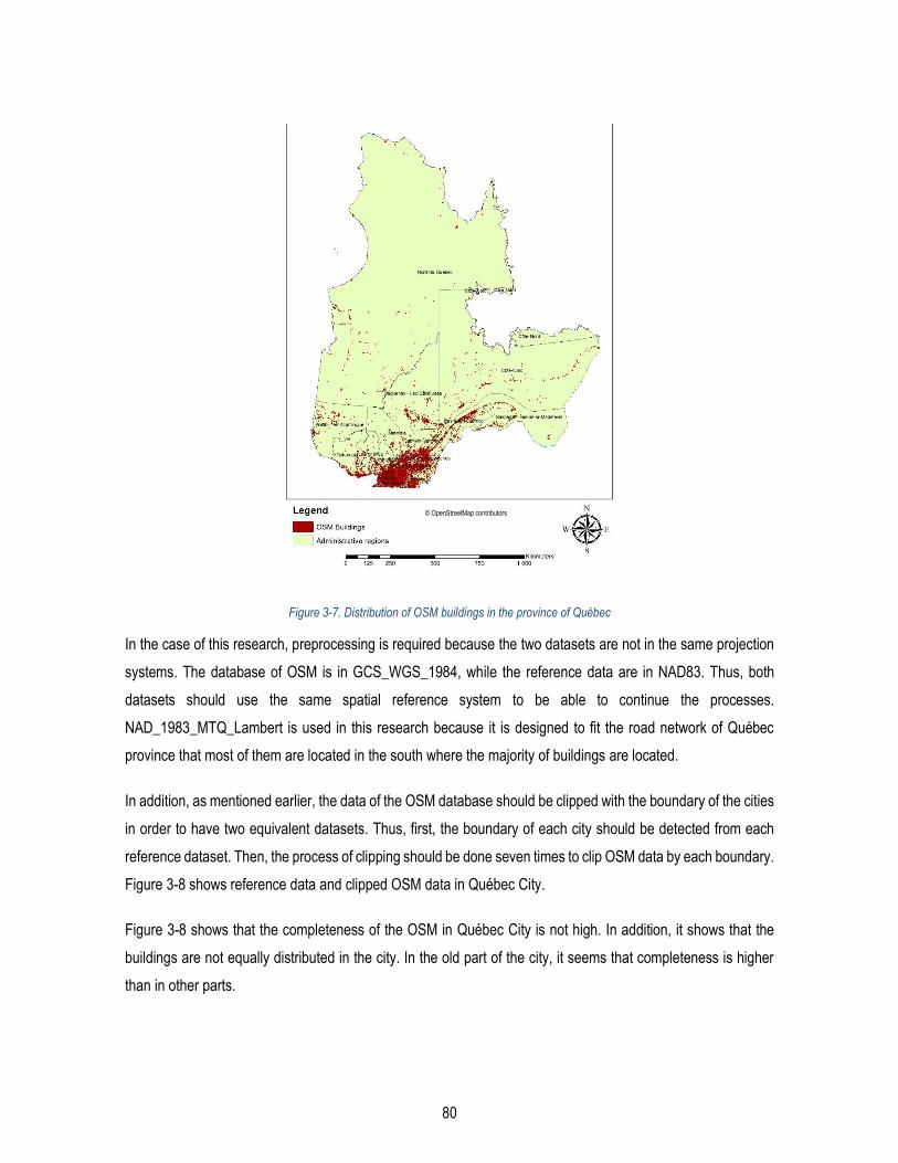
80
Figure 3-7. Distribution of OSM buildings in the province of Québec
In the case of this research, preprocessing is required because the two datasets are not in the same projection
systems. The database of OSM is in GCS_WGS_1984, while the reference data are in NAD83. Thus, both
datasets should use the same spatial reference system to be able to continue the processes.
NAD_1983_MTQ_Lambert is used in this research because it is designed to fit the road network of Québec
province that most of them are located in the south where the majority of buildings are located.
In addition, as mentioned earlier, the data of the OSM database should be clipped with the boundary of the cities
in order to have two equivalent datasets. Thus, first, the boundary of each city should be detected from each
reference dataset. Then, the process of clipping should be done seven times to clip OSM data by each boundary.
Figure 3-8 shows reference data and clipped OSM data in Québec City.
Figure 3-8 shows that the completeness of the OSM in Québec City is not high. In addition, it shows that the
buildings are not equally distributed in the city. In the old part of the city, it seems that completeness is higher
than in other parts.
© OpenStreetMap contributors

81
Figure 3-8. Reference data and clipped OSM data in Québec City.
Figure 3-9. Reference data and OSM data on the campus of Laval University
© OpenStreetMap contributors
© OpenStreetMap contributors
© Ville de Québec
© Ville de Québec

82
Figure 3-9 illustrates that the campus of the university is almost completely mapped, while the neighborhood
that is located in the south of the university is not mapped very well.
The next step of preprocessing is removing the polygons that are smaller than 20m2 because most likely they
are not representing buildings. Given that the majority of the building footprints in OSM are created by digitizing
the aerial images, it is likely that a parking or swimming pool is categorized as a building due to the low resolution
of Bing map aerial images. By deleting very small polygons, we avoid the risk of inaccurate results. The number
of deleted polygons in Longueuil, Québec, Repentigny, Rouyn-Noranda, and Shawinigan is 1134, 79550, 26 ,
2940, and 21 , respectively. It is important that the researchers delete very small polygons because in some
cities there are huge numbers of outliers that can affect the results.
Feature Matching
As mentioned in the previous sections, previous researches used mainly two methods for feature matching 1)
centroid method and 2) overlay method. None of these methods is accurate because they may match the wrong
features if the polygon is displaced or has a considerable shape dissimilarity. To end this problem, we proposed
an algorithm that first finds a group of candidate polygons (features) and then measures the shape similarity
between any possible subgroup of this group and the target polygon. Therefore, the matching is not only based
on the overlay percentage of centroid intersection. It is in fact, based on both overlay and shape similarity. Thus,
our proposed method improves previous methods by adding the shape similarity checking to the matching
algorithm. In this research, this method is used to find the corresponding polygons.
In order to assess the precision of this method, we have checked a number of buildings manually to see how
many percent of them are matched correctly using the proposed method. There is no automatic method to find
out this percentage because there is no method that does the feature matching with 100% accuracy. Among
100 randomly selected polygons in OSM, 8 of them were not matched correctly with the overlay method. Then,
out of 8, 6 of them were correctly matched using the proposed method. It can be concluded that the error in the
overlay method is less than 10%. However, the proposed method is powerful in fixing the majority of those errors.
Evaluating the completeness
As mentioned earlier, there are two main methods for calculating the completeness of the OSM database. The
unit-based method and the object-based method. The unit-based method compares the total number or area of
the buildings in the two databases, while the object-based method first finds the corresponding features and
then, it calculated the completeness based on the matching objects. In the previous researches, two main
methods have been used for feature matching: overlay and centroid methods. Neither of the two feature
matching methods are precise in the case of OSM feature matching. In this study, first, a more precise feature
matching algorithm was proposed. Then, the two databases were matched using this method. Finally, the

83
completeness was calculated using the corresponding features. In addition, the results of unit-based
completeness assessment methods were calculated in order to compare the two methods.
Unit-based completeness evaluation
In this section, the completeness of the building footprints for OSM is evaluated by comparing it to the reference
data set. Two measures of completeness are calculated: based on the number of the buildings in the two
databases and based on the total area of the buildings in the two databases. Table 3-3 shows the unit-based
completeness of the cities.
Table 3-3. Unit-based completeness for the selected cities in the Québec Province
OSM Reference Completeness
ID City No. of B. Area No. of B. Area Based on
Number
Based on
Area
Ratio
1 Repentigny 1693 1183340 24133 4527833 7% 26% 3.7
2 Québec 14409 10479443 160485 30849277 9% 34% 3.7
3 Shawinigan 384 828649 19115 3806090 2% 22% 11
4 Rouyn-
Noranda
421 400208 26686 3664484 1.5% 11% 7.3
5 Longueuil 3027 3865171 61304 10622880 5% 36% 7.2
Table 3-3 shows that there is a considerable difference between the completeness calculated by the total number
of the buildings and the completeness calculated based on the total area of the buildings in the two databases.
In order to explain these findings, one should pay attention to the behavior of the OSM contributors. One possible
hypothesis is that the contributors tend to digitize the largest objects. For example, a large shopping center
attracts more attention than a small house in a residential neighborhood.
In order to test if this hypothesis is true or not, we have to find out if the large buildings are digitized more than
the small ones or not. Table 3-4 shows the average area of the building footprints for the reference database
and the OSM database.

84
Table 3-4. Average area of the building footprints in OSM and in the reference databases
ID City Avg. Area in OSM (m2) Avg. Area in Ref. (m2) Ratio
1 Repentigny 698 187 3.7
2 Québec 727 192 3.7
3 Shawinigan 2157 199 10.8
4 Rouyn-
Noranda
950 137 6.9
5 Longueuil 1276 173 7.3
Table 3-4 shows that almost in all cities, the average area of the corresponding buildings in OSM is considerably
larger than the average area of the buildings in the reference database. More precisely, the ratio between the
average area of the buildings in the two databases in table 3-4 is very similar to the ratio between the two
completeness measures of the table 3-3. In other words, the difference between the two measures of
completeness can be due to the fact that the larger buildings are mapped better in OSM while smaller ones are
missing. This hypothesis that, the larger buildings are better mapped, will be evaluated using the statistical
methods in the next sections.
The measure of completeness should be chosen based on the application. For example, if we want to know how
many percentages of the buildings are mapped in OSM, we will use the measure based on the number. If the
area covered by OSM buildings matters in the target application, then the completeness measure based on the
total area should be used. The authors believe that both of these measures can provide insight into how complete
OSM is in defference cities in Québec Province. However, users of the OSM data should pay attention that the
average area of the buildings in OSM is considerably larger than the average area of the buildings in the
reference dataset. Consequently, this difference can cause a noticeable difference between the two
completeness measures.
Generally, the completeness of the buildings in the cities of the province of Québec is less than 50% based on
both methods. It means that the OSM database is not complete yet and more contributions are required for
having a higher completeness. Furthermore, the comparison between the cities indicates that larger cities
(Québec and Longueuil) are slightly more complete than small cities. The building footprint database of OSM is

85
far less complete than its road database because the road network is almost complete in urban areas of the
province.
Object-based completeness evaluation
Object-based completeness assessment is more realistic because it finds the corresponding features first and
then calculates the completeness based on the corresponding features. In this research, a more accurate
method of feature matching is applied in order to improve the accuracy of the matching. Then, the types of
relationships (correspondings) between the features are evaluated. For the purpose of this section, the “OSM –
Reference” relation type of “0 : 1” is considered as an omission and the relation type “1 : 0” is considered as a
commission. In addition, only ”1 : 1” relation is considered as correct representation and object-based
completeness is calculated based on the number of “1 : 1” relations. Table 3-5 shows the completeness of the
Québec cities based on the object-based method.
Table 3-5. The object-based completeness assessment for the cities of the province of Québec
ID City Omission (no. of B.) Commission (no. of B.) Completeness Total No. of B. in
the reference
1 Repentigny 22470 24 6.7% 24133
2 Québec 147544 1164 7.1% 160485
3 Shawinigan 18840 138 1.05% 19115
4 Rouyn-
Noranda
26383 127 1.01% 26686
5 Longueuil 58946 822 3.2% 61304
The object-based results are similar to the results of the unit-based method while counting the number of
buildings in the two databases. The reason is that the majority of the buildings are well-mapped by the OSM
contributors and as a consequence, a few percentage of them are eliminated in feature matching step.
Evaluating completeness for each grid
In order to investigate the spatial distribution of the completeness in more detail, a grid of rectangles is created
and the calculations are done for each grid cell separately. In other words, firstly, the measures of quality and
the indicators of quality will be calculated for a 1km*1km area (each grid cell). Then, each cell will be used as
input data for the statistical analysis. Then, we can know whether or not statistically, there is a correlation

86
between the measures of the quality and its indicators. A grid of 1km*1km is created for each city and is imported
into the database. Next, the following measures related to completeness are calculated for each grid:
• Unit-based: 1- completeness based on the area of the buildings 2- completeness based on the
number of the buildings
• Object-based: 1- Omission 2- Commission 3- Completeness
Figure 3-10. The 5 measures of quality for each grid in Québec City
© OpenStreetMap contributors
© Ville de Québec

87
The codes for calculating these measures were written in SQL. These 5 measures of completeness are
calculated for each grid cell in each city. These cells are then used for statistical analysis. Figure 3-10 illustrates
the values of these measures for Québec City. This figure illustrates two unit-based measures and three object-
based measures of quality. The completeness is higher in the center of the city in comparison to its suburbs. In
general, omission is much more frequent than commission in the city.
Evaluating the positional accuracy
In this research, the positional accuracy is calculated by comparing the position of the centroid of the polygon in
OSM to the position of the centroid of the reference polygon. The distance between the two centroids is
calculated and used as a measure of the positional accuracy. Therefore, if the OSM building is digitized exactly
in the same position as the reference building, the positional accuracy is high and the distance between the two
centroids is zero. If the OSM building is far from the correct position, then the distance is large and the positional
accuracy is low. Therefore, there is a reverse relation between positional accuracy and the distance of the two
centroids. Figure 3-11 illustrates the centroid of the buildings for a sample area.
Figure 3-11 OSM buildings in and in the reference database with their centroids
The average distance between the two centroids is calculated for each city. Only the buildings with a “1:1”
relation are included in the calculations. Figure 3-11 illustrates the average distance between the centroids for
each city of the province of Québec.

88
Figure 3-12. Average distance between the centroid of the OSM buildings and their corresponding reference building (m)
The positional accuracy of the building footprints was calculated using the PostGIS extension of PostgreSQL
database. Generally, the positional accuracy of the building footprints is acceptable considering the fact that the
quality of the aerial images is about 4m. The highest quality is related to the OSM database for Repentigny
(2.1m) and the lowest quality is for Shawinigan (5.7m). In Québec City, the average distance between the OSM
centroid and the corresponding reference centroid is about 3.4m which is acceptable with respect to the
positional quality of the aerial images.
The distance between the two centroids can provide information about how precise the OSM polygons are
positioned in comparison to the corresponding Québec polygons. However, it cannot provide information about
whether or not the building footprints are shifted towards any direction or they are scattered randomly. Therefore,
in this step, the scatter diagram of the displacements was analyzed to find possible patterns in the displacements
or not. Figure 3-12 shows the scatter diagram of the displacements. The displacement is calculated based on
the comparison of the position of OSM building’s centroid to the corresponding building’s centroid. Figure 3-13
illustrates that in some cities the displacement is not random. For example, in Québec City, on average, the
buildings are shifted towards the northeast, while in Repentigny, the buildings are shifted towards the northwest.
I believe that the aerial image angle can cause some radial displacement in the position of the top of the
buildings. In fact, when the buildings are far from the image center, the top of the buildings is printed in a different
position than their footprint. Therefore, one possible explanation can be the distance of the buildings from the
center of the image. In that case, in each photo, the buildings should be displaced in a specific direction. This
issue can be further investigated by measuring it for each grid cell.

89
Figure 3-13. Scatter diagrams of the displacement of the centroids of OSM buildings

90
Evaluating positional accuracy for each grid
In this section, the average positional accuracy will be calculated for each grid cell because this measure will be
used in the next sections for calculating the correlation between the positional accuracy of the buildings and
indicators of quality. The average distance between the centroids is calculated for each grid in PostGIS. The
following figure shows the average positional accuracy for each grid in Québec City.
Figure 3-14. Average positional accuracy for each grid cell in Québec City
Based on Figure 3-14 the positional accuracy is almost acceptable in different parts of the city. In order to answer
the question that whether or not the positional accuracy decreases with the distance from the center of the city,
this result should be used to measure the correlation between the two variables.
Evaluating the shape accuracy
As mentioned earlier, the building footprints of OSM are mainly digitized by the contributors of OSM. Therefore,
the shapes of the digitized polygons are not exactly similar to the corresponding shapes of the footprint of the
buildings in the reality. In this section, four measures, that previous researches used for shape accuracy, will
be calculated for evaluating the shape accuracy of the OSM building footprints in the selected cities of Québec
Province. In fact, these measures provide us insight into how similar the OSM building footprints are to the
corresponding footprints in reality (in the reference database).
© OpenStreetMap contributors
© Ville de Québec

91
Calculating the area ratio
The ratio between the area of the building footprint in OSM and the area of the corresponding building in the
reference building is a measure that shows how two polygons are similar. This measure is a basic measure and
easy to calculate. Figure 3-15 illustrates the ratio of the area of the building footprints between the two databases.
Figure 3-15. Area ratio between the OSM buildings and their corresponding reference building
Figure 3-15 shows that the average area of OSM buildings is almost equal to the average area of the
corresponding buildings in the reference database. In other words, the average ratio between the two areas is
almost 1 for all cities. Among the cities, Rouyn-Noranda has the highest ratio and Repentigny has the lowest
ratio. It means that the polygons in Repentigny are on average more similar in terms of area than in Rouyn-
Noranda. It is important to know that this area ratio is calculated between the buildings that have a 1:1 relation
with the buildings of the reference database. The area ratio between all the buildings in the two databases is not
even close to 1.
Calculating Compactness
Compactness is a measure that was proposed in previous researches for measuring the shape similarity
between OSM buildings and reference buildings. The compactness of a polygon indicates the degree to which
the polygon is similar to a circle. If the buildings in OSM have similar compactness to the buildings in the
reference database, then, the two buildings are more similar. Compactness does not indicate the exact similarity
between the two sets of polygons. However, this measure can provide an insight into how the two polygons are
similar. Figure 3-16 illustrates the compactness values for the cities.
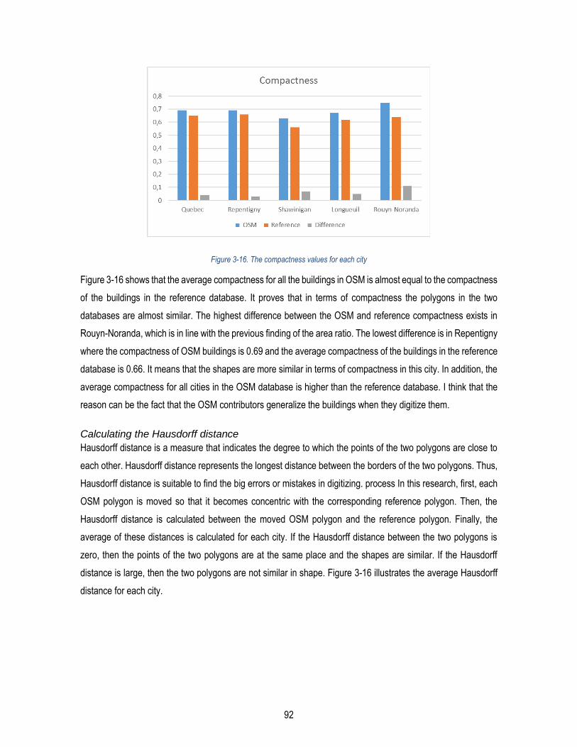
92
Figure 3-16. The compactness values for each city
Figure 3-16 shows that the average compactness for all the buildings in OSM is almost equal to the compactness
of the buildings in the reference database. It proves that in terms of compactness the polygons in the two
databases are almost similar. The highest difference between the OSM and reference compactness exists in
Rouyn-Noranda, which is in line with the previous finding of the area ratio. The lowest difference is in Repentigny
where the compactness of OSM buildings is 0.69 and the average compactness of the buildings in the reference
database is 0.66. It means that the shapes are more similar in terms of compactness in this city. In addition, the
average compactness for all cities in the OSM database is higher than the reference database. I think that the
reason can be the fact that the OSM contributors generalize the buildings when they digitize them.
Calculating the Hausdorff distance
Hausdorff distance is a measure that indicates the degree to which the points of the two polygons are close to
each other. Hausdorff distance represents the longest distance between the borders of the two polygons. Thus,
Hausdorff distance is suitable to find the big errors or mistakes in digitizing. process In this research, first, each
OSM polygon is moved so that it becomes concentric with the corresponding reference polygon. Then, the
Hausdorff distance is calculated between the moved OSM polygon and the reference polygon. Finally, the
average of these distances is calculated for each city. If the Hausdorff distance between the two polygons is
zero, then the points of the two polygons are at the same place and the shapes are similar. If the Hausdorff
distance is large, then the two polygons are not similar in shape. Figure 3-16 illustrates the average Hausdorff
distance for each city.

93
Figure 3-17. Average Hausdorff distance for each city (m)
Figure 3-17 shows that the building footprints in Repentigny have the lowest Hausdorff distance, while the
building footprints in Rouyn-Noranda have the highest Hausdorff distance. It means that the shape of the
buildings in OSM and reference databases are more similar in Repentigny and less similar in Rouyn-Noranda.
Moreover, the Hausdorff distance in Québec, Repentigny, and Longueuil is less than 4m, which means that the
average value of maximum dissimilarity between the two shapes is less than 4m. Thus, in these three cities, the
shape accuracy of the buildings is better than Shawinigan and Rouyn-Noranda.
Calculating the average distance
Hausdorff distance represents maxim um distance between the corresponding points of the two polygons.
Therefore, this measure represents the errors and not the average dissimilarity between the two shapes. Thus,
in this section, the average distance method is used to measure how similar the two shapes are. In the first step,
the OSM polygon is moved so that it becomes concentric with the reference building. Then, the average distance
is calculated between the OSM polygon and its corresponding polygon in the reference database. Figure 3-18
illustrates the average value of the average distance for each city.

94
Figure 3-18. Average value of the average distance for each city (m)
Figure 3-18 shows that Rouyn-Noranda has the highest average distance and Repentigny has the lowest. The
average distance for all cities is less than 1m. This finding is in line with what the authors expected because the
average distance should be smaller than Hausdorff distance. The reason is that Hausdorff distance is the
maximum distance and it is affected by a small dissimilarity in the shapes, while the average distance represents
the average similarity of the two shapes and not just the similarity of the small part of the polygons. These results
are also in line with the results of the previous steps where Rouyn-Noranda seems to have the least shape
accuracy based on different measures.
Calculating shape accuracy parameters for each grid cell
In this section, each of the above-mentioned measures will be calculated for each grid cell. A gird of 1km*1km
is used in PostGIS. The codes are written in SQL and are available for future studies. Figure 3-19 illustrates the
four measures of shape accuracy for Longueuil.
Figure 3-19 shows the distribution of the shape accuracy measures in Longueuil. In order to find out whether or
not shape accuracy measures are related to indicators such as population, income, and other criteria, statistical
tests should be done.

95
Figure 3-19. Shape accuracy measures for the city of Longueuil
© OpenStreetMap contributors
© Ville de Longueuil

96
Evaluating the attribute accuracy
In this step, the attributes of the OSM buildings that are stored in the form of tags are evaluated. The most
important attribute is the name of the building and it is evaluated in this section. All attributes in OSM are stored
in the form of key=value pairs. TagInfo (https://taginfo.openstreetmap.org/) is a website that provides us with the
most frequent tags that exist for a key [60]. This is a good source for evaluating different tags that the contributors
used so far to describe a geographic location. Figure 3-20 illustrates the tags that are related to buildings. The
other tags include information about the number of floors, use, and color of the building.
In this section, the attributes of OSM buildings are compared with the attributes of the buildings in the reference
database. This comparison is made by the Levenshtein distance algorithm. This algorithm finds the number of
deletions, insertions, and substitution that is required to change string A to string B [93]. Therefore, greater
value for the Levenshtein distance indicates that the two strings are not similar, while a Levenshtein distance of
0 indicates that the two strings are equal. In this section, first, the two sets of the data are matched using the
proposed algorithm. Then, the Levenshtein distance between the name of the building in OSM and the name of
the building in the reference database is calculated. The low value of Levenshtein distance shows good attribute
quality.
Figure 3-20. taginfo results for the tag "building=yes" (source: https://taginfo.openstreetmap.org/)

97
In our databases, only the two cities of Rouyn-Noranda and Repentigny have the field of “nom_batim” which
represents the name of the building in the reference data. Thus, the comparison is only possible for these two
cities and not for others. Among the buildings of Repentigny, only 238 and among the buildings of Rouyn-
Noranda only 113 buildings have a name. In fact, other buildings even in the reference database does not have
a name. It can be normal, because only a few percentage of the buildings have a name in reality. But this
percentage is not considerable and we do not enter it in the statistical calculations. The average Levenshtein
distance for Repentigny and Rouyn-Noranda is 2.4 and 3.3, respectively. It means that in average the names of
the buildings had 2 to 3 letters different from the real name. In addition, it means that building names in
Repentigny is more accurate than Rouyn-Noranda.
Statistical analysis
The purpose of this section is to find whether there is a correlation between the measures of the quality and
criteria such as income and population. Therefore, the measures of the quality as well as the criteria that we
wanted to test, are calculated for each grid cell. Then, the correlation is measured to find out how correlated is
quality to these criteria. The criteria that are selected in this research are either mentioned by previous
researches or were observed during this research by the authors. For example, one of these variables (or
indicators of quality) is the density of the buildings in each region. [10] mentioned that there is an almost linear
relation between the density of the OSM buildings in each region and the completeness of the buildings in that
region. Therefore, the density of OSM data can be considered as a potential indicator that provides an insight
into the quality of OSM for those countries where there is no reference (authoritative) data to evaluate the quality
of the OSM. In this research, the finding of [10] is taken into account and also it is further expanded for other
measures of the quality such as completeness based on the number of the commissions, omissions, shape
accuracy and positional accuracy. Therefore, the hypothesis is that density has a relation not only with
completeness but also with other measures of quality.
Another criterion (indicator) that previous researches mentioned that have a relation with OSM quality is the
population [9], [96]. In [4] authors realized that there is a relation between the population and the positional
accuracy of the OSM buildings. However, the previous researches just evaluated the relation between the
completeness and the population of the region and there is no research to investigate the relationship between
population and the other measures of the quality shape accuracy or commission and omission. Thus, in this
research, the relation with population is investigated with all the measures of the quality to provide complete
information about the impact of population on different aspects of the quality.

98
[70] noticed that OSM building completeness increases by economic factors and the length of the OSM roads
in that region. They argued that probably in economically developed areas there are more Internet users and
OSM contributors, while in poor areas the access to the internet may not be easy. Furthermore, [70] argued that
OSM is more complete in touristic areas and commercial centers. [23] found that OSM commercial and
government buildings in Ottawa are more complete than the residential buildings. Therefore, the type of building
may have a relation with the quality of the OSM building. In this research, the correlation between the quality of
OSM building data with the average income of the region, OSM road length in the grid cell is calculated. In
addition, [25] found out that areas with commercial and touristic buildings are more complete than other areas.
Therefore, in this research, the relation between the number of points of interests in each grid cell and the quality
is investigated.
In addition, during this research authors realized that bigger buildings seem to be better mapped in OSM than
small buildings. In order to find out whether it is right or not the correlation between the measures of quality and
the size of the buildings is calculated. Figure 3-21 illustrates the variables that correlation is calculated between
them. On the left side of the potential indicators and on the right side of the Figure 3-21 the measures of quality
are illustrated. In this step, the correlation between the two sets of variables is calculated. Spearman's rank
correlation coefficient is used in this research because it can detect any monotonic relation between the two
variables. If the increase of one of the variables, increases the other one or vice versa, then the two variables
have a monotonic relation. During the previous steps, 10 measures related to the 3 quality parameters are
calculated for each grid. 6 variables of potential indicators are also calculated for each grid.

99
Figure 3-21. Calculating the correlation between the quality measures and potential indicators
Table 3-6 shows the value of Spearman’s correlation coefficient between the quality measures and quality
indicators. Table 3-6 shows that among different quality measures, the measures related to completeness have
a stronger correlation with quality indicators than positional accuracy and shape accuracy. A potential
explanation is that the completeness in most of the grids is less than 10% and for the grids that are far from the
center of the city, the completeness is 0. In those areas, there are no OSM buildings and therefore the values of
shape accuracy and positional accuracy for those areas are not defined (null value). Thus, the completeness is
defined (but is equal to 0) in the areas that the population is low or the areas that are very far from the center of
the city, but the other measures of quality are not even defined in those areas. Consequently, we can better
analyze the impact of the population on completeness than on positional and shape accuracies.
Moreover, Table 3-6 shows that the correlation between the completeness and all quality indicators is higher
than 50%, except income, which means that all those variables can be used as indicators of completeness. The

100
values of correlation for completeness and omission are usually the opposite of each other which is because
these two measures represent two opposite concepts. Among the quality indicators, the density of OSM
buildings has the highest correlation with completeness measures.
The positional accuracy has the highest correlation with the density of roads and then the density of buildings.
The values of the correlation between the positional accuracy (distance between the two centroids) of the density
of OSM roads and buildings are negative, which means that the increase of density of buildings or roads
decreases the distance between the two centroids (improvement of positional accuracy). In addition, there is a
correlation of more than 40% between positional accuracy and shape accuracy which means each of them can
be used as an indicator of the other one. This finding is new and non of the previous researches mentioned it so
far.
Among the measures of shape accuracy, area ratio and compactness difference are the ones with lower
correlations. One explanation is that these two measures are not precise measures of quality and they are rough
measures. Therefore, their values do not change dramatically with the change of quality indicators. On the other
hand, the correlation values of Hausdorff distance and average distance are almost similar because these two
measures of quality are almost representing the same concept.
Hausdorff distance is affected by extreme shape errors but the average distance value is the average distance
between the corresponding points of the two polygons and is less affected by extreme cases. Consequently,
average distance has a stronger correlation with all 6 quality indicators than Hausdorff distance.
The correlation between Hausdorff distance and average distance is 86% which means they can be used as
an indicator of each other. Furthermore, there is a stronger correlation between shape accuracy measures and
the density of buildings and the distance to the center of the city. Thus, the density of buildings and distance to
the center of the city are better indicators for shape accuracy than population and income. The negative value
of the correlation between the density of buildings and average distance means that the increase of the density
of OSM buildings decreases the distance between the two polygons and increases the similarity of the two
shapes (increases shape accuracy). The key for interpreting Table 3-6 is illustarated in Figure 3-21.

101
Table 3-6. Spearman’s rank correlation between the quality measures and quality indicators
variable A B C D E F G H I J 1 2 3 4 5 6
A
1
-0.6
6
-0.9
9
-0.9
9
-0.9
9
0.1
1
0.0
4
0.1
3
0.1
9
0.1
7
-0.5
7
-0.1
6
-0.6
1
-0.9
9
-0.7
1
0.5
3
B
* 1
0.6
5
0.6
5
0.6
5
0.0
3
-0.0
4
-0.0
8
-0.1
0
-0.1
1
0.3
9
0.0
8
0.4
4
0.6
7
0.5
6
-0.3
6
C
* * 1
0.9
9
0.9
9
-0.1
4
-0.0
2
-0.1
7
-0.2
5
-0.2
2
0.5
4
0.1
6
0.6
0
0.9
8
0.6
8
-0.5
2
D
* * * 1
0.9
9
-0.0
5
0.1
0
-0.1
2
-0.0
1
-0.0
2
0.5
4
0.1
5
0.6
0
0.9
8
0.6
9
-0.5
2
E
* * * * 1
-0.1
4
-0.0
1
-0.1
7
-0.2
4
-0.2
2
0.5
4
0.1
5
0.6
0
0.9
8
0.6
9
-0.5
2
F
* * * * * 1
-0.0
1
0.1
8
0.4
9
0.4
3
-0.0
9
-0.0
3
-0.1
1
-0.1
3
-0.0
7
0.0
0
G
* * * * * * 1
-0.0
2
0.0
7
0.0
6
0.0
0
-0.0
8
0.0
2
0.0
5
-0.0
0
-0.1
3
H
* * * * * * * 1
0.4
1
0.4
1
0.0
6
-0.1
4
0.0
4
-0.0
6
0.0
2
-0.0
6
I
* * * * * * * * 1
0.8
6
-0.0
4
-0.1
6
-0.0
2
-0.2
1
-0.1
3
-0.1
4
J
* * * * * * * * * 1
-0.0
6
-0.1
8
-0.0
5
-0.2
2
-0.1
8
-0.1
7

102
1
* * * * * * * * * * 1
0.4
6
0.7
2
0.5
8
0.5
6
-0.8
3
2
* * * * * * * * * * * 1
0.2
9
0.1
6
0.1
8
-0.5
1
3
* * * * * * * * * * * * 1
0.6
3
0.5
9
-0.6
4
4
* * * * * * * * * * * * * 1
0.7
3
-0.5
4
5
* * * * * * * * * * * * * * 1
-0.4
8
6
* * * * * * * * * * * * * * * 1
In this section, the correlation between size of the buildings and the quality measures is evaluated. In this step,
the correlation between the size of the footprint and completeness is measured for each grid cell because it is
not possible to measure it for each feature. However, the correlation between size and positional accuracy and
shape accuracy are calculated for each feature. The relationship between the size of the building (the area of
the footprint) and the quality measures is evaluated using Spearman’s rank correlation coefficient. Figure 3-22
illustrates the correlation coefficient between size and quality measures. Considering the fact that bigger
buildings are mapped with less absolute accuracy, relative accuracy is also measured to better describe the
behavior of quality measure in relation to the size of the footprint. In order to calculate the relative positional
accuracy, the distance between the two centroids is divided by the radius of the equivalent circle. The radius of
the equivalent circle is calculated by finding the radius of the imaginary circle that has the same area as the
footprint. In large buildings, the distance between the two centroids is larger when we divide it by the radius of
the shape, then the relative positional accuracy will be calculated.

103
Table 3-7 Correlation between the size of the buildings' footprints and quality measures
Grid-based Feature-based calculation
Absolute Relative
Indicator Completeness Positional Accuracy Shape Accuracy Positional Accuracy Shape Accuracy
Size 0.57 0.19 0.40 -0.48 -0.27
Table 3-7 shows that there is a very strong correlation between the completeness and average size of the
buildings’ footprints in each grid. Bigger buildings attract more attention and it is more likely that one of the
contributors decides to add them to the map. There is a correlation of 0.19 between absolute positional accuracy
and the size of the buildings. It means that the centroids of the bigger buildings are moved more than small
buildings. However, the relative positional accuracy, which is the distance between the two centroids divided by
the radius of the polygon (radius of a circle with the same area), has a correlation of -0.48 with size. It means
that bigger buildings are relatively better digitized in OSM. In addition, absolute shape accuracy has a correlation
of 0.40 with the size of the buildings. It means that the similarity between the real shape of the building and its
shape in OSM reduces when the size increases. The author believes that bigger buildings are mapped with
fewer details. When the size of buildings increases, people do not digitize the details of the footprints. However,
the relative shape accuracy improves when the size of the buildings footprints increases.
Statistical hypothesis testing
The correlation between quality measures and quality indicators is calculated in the previous section. However,
these correlation values are not sufficient to accept or reject a positive association (relationship) between the
quality measures and quality indicators. In this research, statistical hypothesis testing is used to determine
whether a significant positive association exists between the quality measures and quality indicators. The H0
and H1 hypotheses are as follows:
• H0: There is no significant positive association between the quality measures and quality indicators
(variables of Table 2-2).
• H1: There is a significant positive association between the quality measures and the quality indicators.

104
This test is a one-tail test and the number of pairs is 2,843 (which is the number of grid cells in all cities).
Therefore, the critical value of Spearman’s correlation test is ρc=0.037 at the significance level of 0.05. It meas
that any correlation greater than 0.037 rejects the null hypothesis and proves a positive association between the
two variables. Table 3-8 shows the results of statistical test for the variables of Table 3-6. The letter Y means
that a positive association is accepted, while letter N means that the positive association is not accepted. The
key to interpret Table 3-8 is illustrated in Figure 3-21.
Table 3-8. Result of Spearman’s correlation test between the quality measures and quality indicators
variable A B C D E F G H I J 1 2 3 4 5 6
A Y Y Y Y Y Y Y Y Y Y Y Y Y Y Y Y
B * Y Y Y Y N N Y Y Y Y Y Y Y Y Y
C * * Y Y Y Y N Y Y Y Y Y Y Y Y Y
D * * * Y Y Y Y Y N N Y Y Y Y Y Y
E * * * * Y Y N Y Y Y Y Y Y Y Y Y
F * * * * * Y N Y Y Y Y N Y Y Y N
G * * * * * * Y N Y Y N Y N Y N Y
H * * * * * * * Y Y Y Y Y Y Y N Y
I * * * * * * * * Y Y Y Y N Y Y Y
J * * * * * * * * * Y Y Y Y Y Y Y
1 * * * * * * * * * * Y Y Y Y Y Y
2 * * * * * * * * * * * Y Y Y Y Y
3 * * * * * * * * * * * * Y Y Y Y
4 * * * * * * * * * * * * * Y Y Y
5 * * * * * * * * * * * * * * Y Y
6 * * * * * * * * * * * * * * * Y
Table 3-8 shows the result of statistical test between the quality measures and quality indicators. Result of
Spearman’s correlation test shows that the correlation value is significant for most quality indicators.
Completeness has significant correlation with all quality measures except area ratio. Income has a significant
correlation with all quality measures except positional accuracy. The density of OSM buildings has a significant
positive association with all quality measures. The distance to the centre of the city has a positive significant
association with all quality measures except positional accuracy. In addition, omission has a significant positive
correlation with all quality measures and quality indicators. It measn that not only quality indicators such as
population but also quality measures such as completeness and positional accuracy can be used as a proxy for
OSM data omission.

105
Conclusion
This research was focused on the evaluating the quality of OSM building in Québec province in Canada. Building
data are polygonal data. Therefore, the methods that evaluate the quality of building data are not the same as
the methods that are developed for evaluating the quality of roads or points of interest. In this research, firstly, a
literature review is done to find out the methods that are developed for evaluating the quality of polygonal data
and especially buildings data of OSM. Then, the methods were implemented for five cities in the province of
Québec. Next, the quality measures were calculated for the selected cities. Finally, a grid of 1km*1km was
created and the values of quality measures were calculated for each grid. The grid cells were then, considered
as the inputs of statistical analysis. The correlation between the quality measures and the quality indicators are
then calculated.
The results of the study show that the completeness of the cities is between 1% and 7% which means that still
more time is necessary before the OSM buildings database becomes complete. In addition, the completeness
is lower (1%) for small cities such as Rouyn-Noranda, while it is higher (7%) for bigger cities such as Québec
City. In the case of positional accuracy, the distance between the centroid of the OSM feature and the
corresponding reference feature is almost 2.5m to 5.5m. The positional accuracy of the polygons is acceptable
because the resolution of the aerial imagery that is used as the background of the OSM map is about 4m. For
evaluating the shape accuracy, four measures were calculated in this research. According to average distance,
Rouyn-Noranda has the worst and Repentigny has the highest shape accuracy.
The statistical analysis shows that the completeness of OSM buildings database has a strong correlation with
population, income, the density of buildings, the density of roads, and the distance from the center of the city. It
means that these 5 variables can be used as indicators of completeness. In the case of positional accuracy and
shape accuracy, the correlations are lower than completeness. Thus, the 6 variables that are mentioned in this
research are better indicators for completeness than for other measures. In addition, the positional accuracy and
shape accuracy are correlated which means that one of them can be used as an indicator for the other one.
The correlation values between the distance to the center of the city and almost all the quality measures indicate
that the OSM has a better quality in the center of the city. In addition, the results show that the size of the
buildings’ footprints is an important indicator for completeness, relative positional accuracy and shape accuracy.
These findings not only are in line with the previous researches, but also improves them by considering other
indicators such as size of buildings as an indicator of quality measures.

106
Conclusion
In recent years, technological advances, and especially the advent of Web 2.0 changed the way Internet users
use the Internet. Before, users of the Internet were just using the information that was provided to them by the
Internet servers. However, nowadays, the Internet users are able to generate content and send it back to servers
to share with other users. Therefore, the users are both users and producers of the information on the Internet.
The information that users generate can be news, photos, comments, or videos. Recent development in GPS-
enabled devices enabled citizens to generate geographic content such as a trajectory of the path or the polygon
of a park. When users voluntarily generate geographic content and share it on the Internet, they are producing
VGI.
VGI projects usually provide people with tools and technologies that allow them to generate and enrich
geographic content. For example, OSM which is one of the most successful VGI projects, allows contributors to
digitize map features from aerial images. They are also allowed to upload GPS coordinates to specify the position
of a feature. OSM contributors can add tags to add semantic information to map features. There is no rule for
tagging. Contributors are free to add any tags that they think describe the characteristics of the features. In
addition, the OSM contributors may not necessarily be familiar with geographic data collection standards.
Therefore, the geographic content that is generated by the contributors in OSM may not be qualified. Many
researchers tried to evaluate the quality of OSM data.
The quality of geographic data is an issue that attracted the attention of many researchers. There was a debate
in the 2000s about how to describe the quality of geographic data uniquely. ISO organization published a
standard that mentions 6 elements for the quality of geographic data: completeness, logical consistency,
positional accuracy, thematic accuracy, temporal quality, and usability.
This research evaluated the quality of OSM data based on the quality measures that have been proposed by
previous researches. In the first step, a literature review was done to find the quality measures and quality
evaluation methods that have been proposed by previous researches. Then, some of these methods are applied
to evaluate the quality of OSM roads and buildings. Roads are linear features, while buildings are polygonal
features. Thus, the measures that are proposed to evaluate their quality are not necessarily the same. In this
research, the second chapter evaluated the quality of OSM roads, while the third chapter evaluated the quality
of OSM buildings.
In the second chapter, the completeness, positional accuracy, and attribute accuracy of the roads was assessed
for the province of Québec. The road data of OSM was more complete than the authoritative data because in
urban areas it contained stairways, footways, and some other categories that did not exist in the authoritative

107
data. Therefore, a preprocessing was done to delete these roads. Two frequently used methods (increasing
buffer method and double buffer method) were used for evaluating the positional accuracy of roads. Attribute
accuracy was calculated using Levenshtein distance. Levenshtein distance is the number of insertion, deletion,
and modification that is required to change the name of the road in OSM to the name of the road in the reference
database. Finally, the correlation between 5 quality indicators and quality measures was calculated. The
selected quality indicators are: population, income, density of OSM roads, density of OSM buildings and the
number of POIs.
The main conclusions are as follows:
• The completeness of OSM roads in the province of Québec is 32.91%.
• OSM roads are much more complete in urban areas than in other parts of the province.
• 50% of the OSM roads are within 2.5 m of the authoritative roads, while almost 80% of them are within
8 m of the reference roads.
• When the buffer around the reference roads increases beyond 5m, there is no considerable difference
in the percentage of OSM roads that fall within the buffer.
• In terms of the type of road, the lowest positional accuracy is observed for the OSM roads with types
“unknown”, “track_grades” and “path”, while the rest of the road types had a better positional accuracy.
• The positional accuracy of OSM roads is better in urban areas.
• The name of the 87.76% of the OSM roads is exactly matching with the name of the corresponding
roads in the reference database.
• 3.2% of the roads have a Levenshtein distance of 1, which in many cases is caused by typo errors
(especially French accents).
• 5.6% of the roads have a different name in OSM (Levenshtein distance greater than 6).
• The strongest indicators for the road completeness are the density of OSM roads, population, and
income.
• In terms of positional accuracy, population and income are the strongest indicators.

108
• In terms of attribute accuracy, population and income are weak indicators, whilst the density of roads,
the density of buildings, and the number of POIs are not recognized as indicators.
• The correlation between the potential indicators and completeness is higher than the correlation
between them and positional accuracy and attribute accuracy.
The third chapter of this research evaluated the quality of OSM buildings. In this chapter, the completeness,
positional accuracy, shape accuracy, and attribute accuracy of the OSM buildings were evaluated.
Completeness can be calculated in two main ways: 1) with feature matching 2) without feature matching. In this
research, both methods were applied in order to compare the results. A new method of feature matching is
proposed in this chapter. This feature matching algorithm found the corresponding features by comparing the
percentage of the overlap and the similarity of the two shapes. Positional accuracy was evaluated by measuring
the distance between the two centroids. Shape accuracy was measured by area ratio, compactness difference,
Hausdorff distance, and average distance methods. Finally, the correlation between the quality indicators and
quality measures is calculated. The main conclusions of the third chapter are as follows:
• The completeness of the OSM buildings for Québec, Repentigny, Shawinigan, Rouyn-Noranda, and
Longueuil is 9%, 7%, 2%, 1.5%, and 5%, respectively.
• If the completeness is calculated based on the area covered by OSM buildings, then, the completeness
for the above cities is 34%, 26%, 22%, 11%, and 36%, respectively.
• The reason for this difference is that the OSM contributors digitized bigger buildings first. The average
size of the OSM buildings is at least 4 times more than the average size of the reference buildings for
all the cities.
• Positional accuracy of the OSM buildings for Québec, Repentigny, Shawinigan, Rouyn-Noranda, and
Longueuil is 3.4m, 2.1m, 5.7m, 4.6m, and 2.9m, respectively.
• The average distance between the OSM building footprints and the reference building footprints for the
above-mentioned cities is 0.4m, 0.1m, 0.3m, 0.9m, and 0.5m, respectively.
• The correlation between the completeness and population, the density of OSM roads, the density of
OSM buildings, the number of POIs, and the distance to the center of the city is more than 0.50 which
means that these variables can be used as indicators for completeness.

109
• Among the potential indicators, positional accuracy has the strongest correlation with the density of
OSM buildings.
• The correlation analysis showed that the distance to the center of the city and the density of OSM
buildings are the two indicators that can be used for average distance and Hausdorff distance.
• Generally speaking, the indicators have a higher correlation with completeness than with positional
accuracy and shape accuracy.
• There is a high correlation between shape accuracy and average distance and Hausdorff distance
which means that they can be used as an indicator for each other.
• There is a high correlation between the completeness and the average size of the buildings. It means
that size can be used as an indicator for completeness.
• Relative positional accuracy and relative shape accuracy have a high correlation with size which means
that size can be used as an indicator for them.
This research evaluated the quality of OSM roads and buildings in the province of Québec. The correlation
between the potential indicators of quality and the measure of quality is calculated to provide an insight into the
relationships among these variables. The main contribution of this research is providing knowledge about the
indicators of quality. Statistical hypothesis testing was used in this research to find which correlations are
significant and as a consequence those variables can be used as indicators for a quality measure.
For the future researches, the relation between the behavior of the contributors and the quality of their
contribution can be evaluated. In addition, future researches can develop methods and tools for evaluating the
semantic information in OSM. Semantic information is added to OSM as tags. Researchers can evaluate the
accuracy of these tags. Another topic that may interest the future researchers is the full history of OSM. The
history of OSM shows the process in which the OSM database evolved. The relationship between quality
indicators and the evolvement of the OSM database can be analyzed to find out whether indicators such as
population have a relationship with the speed of completeness, the number of edits of the same feature, the
accuracy of semantic information over the time and the speed of updates.

110

111
Bibliographie
[1] V. Antoniou, J. Morley, and M. Haklay, “Web 2.0 geotagged photos: Assessing the spatial dimensions
of the phenomenon,” Geomatica, vol. 64, no. 1, pp. 99–110, 2010.
[2] “Wikipedia Page: Web 2.0,” 2019. http://en.wikipedia.org/wiki/Web_2.0.
[3] M. F. Goodchild, “Citizens as sensors: The world of volunteered geography,” GeoJournal, vol. 69, no.
4, pp. 211–221, 2007, doi: 10.1007/s10708-007-9111-y.
[4] M. Brovelli and G. Zamboni, “A New Method for the Assessment of Spatial Accuracy and
Completeness of OpenStreetMap Building Footprints,” ISPRS Int. J. Geo-Information, vol. 7, no. 8, p.
289, 2018, doi: 10.3390/ijgi7080289.
[5] H. Zhang, “Quality Assessment of the Canadian OpenStreetMap Road Networks,” University of
Western Ontario, 2017.
[6] P. Neis, M. Goetz, and A. Zipf, “Towards Automatic Vandalism Detection in OpenStreetMap,” ISPRS
Int. J. Geo-Information, vol. 1, no. 3, pp. 315–332, 2012, doi: 10.3390/ijgi1030315.
[7] ISO, ISO 19157: Geographic information-data quality. 2013.
[8] V. Antoniou and A. Skopeliti, “Measures and Indicators of Vgi Quality: an Overview,” ISPRS Ann.
Photogramm. Remote Sens. Spat. Inf. Sci., vol. II-3/W5, pp. 345–351, 2015, doi: 10.5194/isprsannals-
II-3-W5-345-2015.
[9] S. Camboim, J. Bravo, and C. Sluter, “An Investigation into the Completeness of, and the Updates to,
OpenStreetMap Data in a Heterogeneous Area in Brazil,” ISPRS Int. J. Geo-Information, vol. 4, no. 3,
pp. 1366–1388, 2015, doi: 10.3390/ijgi4031366.
[10] Q. Zhou, “Exploring the relationship between density and completeness of urban building data in
OpenStreetMap for quality estimation,” Int. J. Geogr. Inf. Sci., vol. 32, no. 2, pp. 257–281, 2018, doi:
10.1080/13658816.2017.1395883.
[11] A. J. Flanagin and M. J. Metzger, “The credibility of volunteered geographic information,” GeoJournal,
vol. 72, no. 3–4, pp. 137–148, 2008, doi: 10.1007/s10708-008-9188-y.
[12] G. Touya, V. Antoniou, A.-M. Olteanu-Raimond, and M.-D. Van Damme, “Assessing Crowdsourced

112
POI Quality: Combining Methods Based on Reference Data, History, and Spatial Relations,” ISPRS
Int. J. Geo-Information, vol. 6, no. 3, p. 80, 2017, doi: 10.3390/ijgi6030080.
[13] V. Antoniou, “User Generated Spatial Content: An Analysis of the Phenomenon and its Challenges for
Mapping Agencies,” UCL (University College London), 2011.
[14] “Wikipedia Page: User-generated content,” 2020. https://en.wikipedia.org/wiki/User-
generated_content.
[15] L. Díaz, C. Granell, M. Gould, and J. Huerta, “Managing user-generated information in geospatial
cyberinfrastructures,” Futur. Gener. Comput. Syst., vol. 27, no. 3, pp. 304–314, 2011, doi:
10.1016/j.future.2010.09.002.
[16] D. Bégin, R. Devillers, and S. Roche, “Assessing Volunteered Geographic Information (Vgi) Quality
Based on Contributors’ Mapping Behaviours,” ISPRS - Int. Arch. Photogramm. Remote Sens. Spat.
Inf. Sci., vol. XL-2/W1, no. June, pp. 149–154, 2013, doi: 10.5194/isprsarchives-xl-2-w1-149-2013.
[17] “Oxford Dictionary.” https://en.oxforddictionaries.com/definition/crowdsourcing (accessed May 07,
2019).
[18] M. F. Goodchild and L. Li, “Assuring the quality of volunteered geographic information,” Spat. Stat.,
vol. 1, pp. 110–120, 2012, doi: 10.1016/j.spasta.2012.03.002.
[19] “Wikipedia Page: Crowdsourcing,” 2020. https://en.wikipedia.org/wiki/Crowdsourcing.
[20] Y. Tong, L. Chen, and C. Shahabi, “Spatial crowdsourcing: challenges, techniques, and applications,”
Proc. VLDB Endow., vol. 10, no. 12, pp. 1988–1991, 2017, doi: 10.14778/3137765.3137827.
[21] F. E. A. Horita, L. C. Degrossi, L. F. F. G. Assis, A. Zipf, and J. P. de de Albuquerque, “The use of
Volunteered Geographic Information and Crowdsourcing in Disaster Management: a Systematic
Literature Review,” in Proceedings of the Nineteenth Americas Conference on Information Systems,
2013, pp. 1–10.
[22] H. Senaratne, A. Mobasheri, A. L. Ali, C. Capineri, and M. (Muki) Haklay, “A review of volunteered
geographic information quality assessment methods,” Int. J. Geogr. Inf. Sci., vol. 31, no. 1, pp. 139–
167, 2017, doi: 10.1080/13658816.2016.1189556.
[23] K. T. Jacobs, “Quality Assessment of Volunteered Geographic Information : An Investigation into the

113
Ottawa-Gatineau OpenStreetMap Database,” Carleton University, 2018.
[24] M. Craglia, F. Ostermann, and L. Spinsanti, “Digital Earth from vision to practice: Making sense of
citizen-generated content,” Int. J. Digit. Earth, vol. 5, no. 5, pp. 398–416, 2012, doi:
10.1080/17538947.2012.712273.
[25] N. Copes, “A Planning based Evaluation of Spatial Data Quality of OpenStreetMap Building Footprints
in Canada,” University of Waterloo, 2019.
[26] M. F. Goodchild and J. A. Glennon, “Crowdsourcing geographic information for disaster response: A
research frontier,” Int. J. Digit. Earth, vol. 3, no. 3, pp. 231–241, 2010, doi:
10.1080/17538941003759255.
[27] M. Moradi, M. R. Delavar, and B. Moshiri, “A GIS-based multi-criteria decision-making approach for
seismic vulnerability assessment using quantifier-guided OWA operator: a case study of Tehran, Iran,”
Annals of GIS, vol. 21, no. 3, pp. 209–222, 2015, doi: 10.1080/19475683.2014.966858.
[28] M. Moradi, M. R. Delavar, and B. Moshiri, “A GIS-based multi-criteria analysis model for earthquake
vulnerability assessment using Choquet integral and game theory,” Natural Hazards, vol. 87, no. 3, pp.
1377–1398, 2017, doi: 10.1007/s11069-017-2822-6.
[29] S. M. Piryonesi and T. E. El-Diraby, “Role of Data Analytics in Infrastructure Asset Management:
Overcoming Data Size and Quality Problems,” J. Transp. Eng. Part B Pavements, vol. 146, no. 2, pp.
1–15, 2020, doi: 10.1061/JPEODX.0000175.
[30] S. M. Piryonesi, “The Application of Data Analytics to Asset Management: Deterioration and Climate
Change Adaptation in Ontario Roads,” University of Toronto, 2019.
[31] W. Yang and L. Mu, “GIS analysis of depression among Twitter users,” Appl. Geogr., vol. 60, pp. 217–
223, 2015, doi: 10.1016/j.apgeog.2014.10.016.
[32] B. Hawelka, I. Sitko, E. Beinat, S. Sobolevsky, P. Kazakopoulos, and C. Ratti, “Geo-located Twitter as
proxy for global mobility patterns,” Cartogr. Geogr. Inf. Sci., vol. 41, no. 3, pp. 260–271, 2014, doi:
10.1080/15230406.2014.890072.
[33] P. Neis, “Measuring the reliability of wheelchair user route planning based on volunteered geographic
information,” Trans. GIS, vol. 19, no. 2, pp. 188–201, 2015, doi: 10.1111/tgis.12087.

114
[34] J. Jokar Arsanjani, M. Helbich, M. Bakillah, J. Hagenauer, and A. Zipf, “Toward mapping land-use
patterns from volunteered geographic information,” Int. J. Geogr. Inf. Sci., vol. 27, no. 12, pp. 2264–
2278, 2013, doi: 10.1080/13658816.2013.800871.
[35] “Oxford Online Dictionary,” 2019. https://en.oxforddictionaries.com/definition/quality (accessed May 15,
2018).
[36] S. C. Guptill and J. L. Morrison, Elements of spatial data quality, vol. 1. Elsevier, 1995.
[37] R. Devillers, Y. Bédard, R. Jeansoulin, and B. Moulin, “Towards spatial data quality information
analysis tools for experts assessing the fitness for use of spatial data,” Int. J. Geogr. Inf. Sci., vol. 21,
no. 3, pp. 261–282, 2007, doi: 10.1080/13658810600911879.
[38] J. J. Arsanjani, P. Mooney, and A. Zipf, “Quality Assessment of the Contributed Land Use Information
from OpenStreetMap Versus Authoritative Datasets,” in OpenStreetMap in GIScience, Springer, 2015,
pp. 37–58.
[39] M. Haklay, “How good is volunteered geographical information? A comparative study of
OpenStreetMap and ordnance survey datasets,” Environ. Plan. B Plan. Des., vol. 37, no. 4, pp. 682–
703, 2010, doi: 10.1068/b35097.
[40] S. Fritz, L. See, M. Brovelli, and C. Campus, “Motivating and Sustaining Participation in VGI,” Mapp.
Citiz. Sens., p. chapter 5, 2016, doi: https://doi.org/10.5334/bbf.e.
[41] C. Chen, “Gamification in a Volunteered Geographic Information context with regard to contributors’
motivations: A case study of OpenStreetMap,” University of Waterloo, 2017.
[42] M. (Muki) Haklay, S. Basiouka, V. Antoniou, and A. Ather, “How Many Volunteers Does it Take to Map
an Area Well? The Validity of Linus’ Law to Volunteered Geographic Information,” Cartogr. J., vol. 47,
no. 4, pp. 315–322, 2010, doi: 10.1179/000870410X12911304958827.
[43] A. L. Ali, Z. Falomir, F. Schmid, and C. Freksa, “Rule-guided human classification of Volunteered
Geographic Information,” ISPRS J. Photogramm. Remote Sens., vol. 127, pp. 3–15, 2017, doi:
10.1016/j.isprsjprs.2016.06.003.
[44] “Wikipedia Page: OpenStreetMap,” 2020. https://en.wikipedia.org/wiki/OpenStreetMap.
[45] M. Haklay and P. Weber, “OpenStreet map: User-generated street maps,” IEEE Pervasive Comput.,
115
vol. 7, no. 4, pp. 12–18, 2008, doi: 10.1109/MPRV.2008.80.
[46] P. Mooney, P. Corcoran, and A. C. Winstanley, “Towards quality metrics for OpenStreetMap,” in
Proceedings of the 18th SIGSPATIAL international conference on advances in geographic information
systems, 2010, p. 514, doi: 10.1145/1869790.1869875.
[47] “OSM Wiki: Statistics,” 2019. https://wiki.openstreetmap.org/wiki/Stats.
[48] D. Bégin, R. Devillers, and S. Roche, “Contributors’ Withdrawal from Online Collaborative
Communities: The Case of OpenStreetMap,” ISPRS Int. J. Geo-Information, vol. 6, no. 11, p. 340,
2017, doi: 10.3390/ijgi6110340.
[49] M. Hacar, B. Kılıç, and K. Şahbaz, “Analyzing OpenStreetMap Road Data and Characterizing the
Behavior of Contributors in Ankara, Turkey,” ISPRS Int. J. Geo-Information, vol. 7, no. 10, p. 400,
2018, doi: 10.3390/ijgi7100400.
[50] “Wiki OSM: Map Features,” 2020. https://wiki.openstreetmap.org/wiki/Map_Features.
[51] L.-A. Siebritz, “Assessing the accuracy of openstreetmap data in south africa for the purpose of
integrating it with authoritative data,” University of Cape Town, 2014.
[52] T. Koukoletsos, “A Framework for Quality Evaluation of VGI linear datasets,” University College
London, 2012.
[53] P. Mooney and P. Corcoran, “The annotation process in OpenStreetMap,” Trans. GIS, vol. 16, no. 4,
pp. 561–579, 2012, doi: 10.1111/j.1467-9671.2012.01306.x.
[54] “Wiki OSM: Taginfo,” 2018. https://wiki.openstreetmap.org/wiki/Taginfo.
[55] J. Almendros-Jiménez and A. Becerra-Terón, “Analyzing the Tagging Quality of the Spanish
OpenStreetMap,” ISPRS Int. J. Geo-Information, vol. 7, no. 8, p. 323, 2018, doi: 10.3390/ijgi7080323.
[56] “Wiki OSM Page: Scientific Tools.” https://wiki.openstreetmap.org/wiki/OSM_Scientific_Tools.
[57] L. Juhász and H. H. Hochmair, “OSM Data Import as an Outreach Tool to Trigger Community Growth?
A Case Study in Miami,” ISPRS Int. J. Geo-Information, vol. 7, no. 3, p. 113, 2018, doi:
10.3390/ijgi7030113.
[58] M. A. Brovelli, M. Minghini, M. E. Molinari, and G. Zamboni, “Positional accuracy assessment of the

116
openstreetmap buildings layer through automatic homologous pairs detection: The method and a case
study,” in International Archives of the Photogrammetry, Remote Sensing and Spatial Information
Sciences - ISPRS Archives, 2016, vol. 41, no. July, pp. 615–620, doi: 10.5194/isprsarchives-XLI-B2-
615-2016.
[59] A. Nasiri, R. Ali Abbaspour, A. Chehreghan, and J. Jokar Arsanjani, “Improving the quality of citizen
contributed geodata through their historical contributions: The case of the road network in
OpenStreetMap,” ISPRS Int. J. Geo-Information, vol. 7, no. 7, p. 253, 2018, doi: 10.3390/ijgi7070253.
[60] N. Davidovic, P. Mooney, L. Stoimenov, and M. Minghini, “Tagging in volunteered geographic
information: an analysis of tagging practices for cities and urban regions in OpenStreetMap,” ISPRS
Int. J. Geo-Information, vol. 5, no. 12, p. 232, 2016, doi: 10.3390/ijgi5120232.
[61] A. Yang, H. Fan, N. Jing, Y. Sun, and A. Zipf, “Temporal analysis on contribution inequality in
OpenStreetMap: A comparative study for four countries,” ISPRS Int. J. Geo-Information, vol. 5, no. 1,
p. 5, 2016, doi: 10.3390/ijgi5010005.
[62] S. Jackson, W. Mullen, P. Agouris, A. Crooks, A. Croitoru, and A. Stefanidis, “Assessing
Completeness and Spatial Error of Features in Volunteered Geographic Information,” ISPRS Int. J.
Geo-Information, vol. 2, no. 2, pp. 507–530, 2013, doi: 10.3390/ijgi2020507.
[63] R. Canavosio-Zuzelski, P. Agouris, and P. Doucette, “A Photogrammetric Approach for Assessing
Positional Accuracy of OpenStreetMap© Roads,” ISPRS Int. J. Geo-Information, vol. 2, no. 2, pp. 276–
301, 2013, doi: 10.3390/ijgi2020276.
[64] M. F. Goodchild and G. J. Hunter, “A simple positional accuracy measure for linear features,” Int. J.
Geogr. Inf. Sci., vol. 11, no. 3, pp. 299–306, 1997, doi: 10.1080/136588197242419.
[65] J. F. Girres and G. Touya, “Quality Assessment of the French OpenStreetMap Dataset,” Trans. GIS,
vol. 14, no. 4, pp. 435–459, 2010, doi: 10.1111/j.1467-9671.2010.01203.x.
[66] D. Zielstra and G. Willem, “Assessing the Quality, Suitability and Usability of User Generated Content
for Routing Applications,” University of Florida, 2014.
[67] R. Hecht, C. Kunze, and S. Hahmann, “Measuring Completeness of Building Footprints in
OpenStreetMap over Space and Time,” ISPRS Int. J. Geo-Information, vol. 2, no. 4, pp. 1066–1091,
2013, doi: 10.3390/ijgi2041066.

117
[68] H. Fan, A. Zipf, Q. Fu, and P. Neis, “Quality assessment for building footprints data on
OpenStreetMap,” Int. J. Geogr. Inf. Sci., vol. 28, no. 4, pp. 700–719, 2014, doi:
10.1080/13658816.2013.867495.
[69] T. Törnros, H. Dorn, S. Hahmann, and A. Zipf, “Uncertainties of completeness measures in
openstreetmap – A case study for buildings in a medium-sized German city,” ISPRS Ann.
Photogramm. Remote Sens. Spat. Inf. Sci., vol. 2, no. 3, pp. 353–357, 2015, doi: 10.5194/isprsannals-
II-3-W5-353-2015.
[70] Y. Tian, Q. Zhou, X. Fu, Y. Tian, Q. Zhou, and X. Fu, “An Analysis of the Evolution, Completeness and
Spatial Patterns of OpenStreetMap Building Data in China,” ISPRS Int. J. Geo-Information, vol. 8, no.
1, p. 35, 2019, doi: 10.3390/ijgi8010035.
[71] I. Lokhat and G. Touya, “Enhancing building footprints with squaring operations,” J. Spat. Inf. Sci., vol.
13, no. 2016, pp. 33–60, 2016, doi: 10.5311/josis.2016.13.276.
[72] H. Fan, A. Yang, A. Zipf, and A. The, “The intrinsic quality assessment of building footprints data on
OpenStreetMap in Baden-Württemberg,” in Flächennutzungsmonitoring VIII Flächensparen-
Ökosystemleistungen-Handlungsstrategien, 2016.
[73] J. Huerta, S. Schade, and C. Granell, “Estimation of Building Types on OpenStreetMap Based on
Urban Morphology Analysis Hongchao,” in Lecture Notes in Geoinformation and Cartography, 2014,
doi: 10.1007/978-3-319-03611-3.
[74] R. Feick and S. Roche, “Understanding the Value of VGI,” in Crowdsourcing geographic knowledge,
Dordrecht: Springer, 2013, pp. 15–29.
[75] A. Graser, M. Straub, and M. Dragaschnig, Progress in Location-Based Services. Springer, 2015.
[76] F. Antunes, M. A. Brovelli, M. Minghini, M. Molinari, and P. Mooney, “Assessing OSM road positional
quality with authoritative data,” VIII Conferência Nac. Cartogr. e Geodésia, no. 2015, pp. 1–8, 2015.
[77] Y. Xu, Z. Chen, Z. Xie, and L. Wu, “Quality assessment of building footprint data using a deep
autoencoder network,” Int. J. Geogr. Inf. Sci., vol. 31, no. 10, pp. 1929–1951, 2017, doi:
10.1080/13658816.2017.1341632.
[78] ISO BAD One, “ISO 19157,” Int. Organ. Stand. Geneva, Switz., vol. 19157, 2013.

118
[79] F. Müller, I. Iosifescu, and L. Hurni, “Assessment and Visualization of OSM Building Footprint Quality,”
in Proceedings of the 27th International Cartographic Conference, 2015.
[80] J. Mondzech and M. Sester, “Quality analysis of OpenStreetMap data based on application needs,”
Cartogr. Int. J. Geogr. Inf. Geovisualization, vol. 46, no. 2, pp. 115–125, 2011, doi:
10.3138/carto.46.2.115.
[81] H. Dorn, T. Törnros, and A. Zipf, “Quality Evaluation of VGI Using Authoritative Data—A Comparison
with Land Use Data in Southern Germany,” ISPRS Int. J. Geo-Information, vol. 4, no. 3, pp. 1657–
1671, 2015, doi: 10.3390/ijgi4031657.
[82] K. Carsten, T. René, and de G. Anton, “Trust as a Proxy Measure for the Quality of Volunteered
Geographic Information in the Case of OpenStreetMap Carsten,” in Lecture Notes in Geoinformation
and Cartography, 2013, vol. 5, pp. 21–37, doi: 10.1007/978-3-319-00615-4.
[83] S. P. Jackson, “Analyzing Contribution Patterns of Volunteered Geographic Point Features in Relation
to Errors and Demographics,” George Mason University, 2014.
[84] C. Barron, P. Neis, and A. Zipf, “A Comprehensive Framework for Intrinsic OpenStreetMap Quality
Analysis,” Trans. GIS, vol. 18, no. 6, pp. 877–895, 2014, doi: 10.1111/tgis.12073.
[85] D. Zielstra and A. Zipf, “A comparative study of proprietary geodata and volunteered geographic
information for Germany,” in 13th AGILE International Conference on Geographic Information Science
2010 Guimarães, Portugal, 2010, vol. 1, pp. 1–15, doi: 10.1119/1.1736005.
[86] P. Neis, D. Zielstra, and A. Zipf, “Comparison of Volunteered Geographic Information Data
Contributions and Community Development for Selected World Regions,” Futur. Internet, vol. 5, no. 2,
pp. 282–300, 2013, doi: 10.3390/fi5020282.
[87] D. Jonietz and A. Zipf, “Defining Fitness-for-Use for Crowdsourced Points of Interest (POI),” ISPRS Int.
J. Geo-Information, vol. 5, no. 9, p. 149, 2016, doi: 10.3390/ijgi5090149.
[88] P. Gil de la Vega, F. J. Ariza-López, and A. T. Mozas-Calvache, “Models for positional accuracy
assessment of linear features: 2D and 3D cases,” Surv. Rev., vol. 48, no. 350, pp. 347–360, 2016, doi:
10.1080/00396265.2015.1113027.
[89] R. B. McMaster, “A Statistical Analysis of Mathematical Measures for Linear Simplification,” Am.
Cartogr., vol. 13, no. 2, pp. 103–116, 1986.

119
[90] A. Olteanu, “Fusion de connaissances imparfaites pour l’appariement de données géographiques :
proposition d’une approche s’appuyant sur la théorie des fonctions de croyance,” Université Paris-Est,
2010.
[91] H. Tveite and S. Langaas, “An accuracy assessment method for geographical line data sets based on
buffering,” Int. J. Geogr. Inf. Sci., vol. 13, no. 1, pp. 27–47, 1999, doi: 10.1080/136588199241445.
[92] M. F. Worboys and M. Duckham, GIS: A Computing Perspective. CRC Press, 2004.
[93] G. Navarro, “A guided tour to approximate string matching,” in ACM computing surveys (CSUR), 2001,
vol. 33, no. 1, pp. 31–88, doi: 10.1145/375360.375365.
[94] “Wikipedia: Quebec Province.” https://en.wikipedia.org/wiki/Quebec.
[95] “Esri. ‘World Imagery’ [basemap]. Scale Not Given. Dec 12, 2009.
https://www.arcgis.com/home/item.html?id=10df2279f9684e4a9f6a7f08febac2a9 (2019-07-02).” .
[96] P. Neis, D. Zielstra, and A. Zipf, “The Street Network Evolution of Crowdsourced Maps:
OpenStreetMap in Germany 2007–2011,” Futur. Internet, vol. 4, no. 1, pp. 1–21, 2011, doi:
10.3390/fi4010001.
[97] “Esri. ‘World Cities’ [basemap]. Scale Not Given. Jun 30, 2013.
https://www.arcgis.com/home/item.html?id=6996f03a1b364dbab4008d99380370ed (2019-07-02).” .
[98] P. Mooney and P. Corcoran, “Characteristics of heavily edited objects in openstreetmap,” Futur.
Internet, vol. 4, no. 1, pp. 85–305, 2012, doi: 10.3390/fi4010285.
[99] “Wiki OSM: Full History Dump,” 2018. https://wiki.openstreetmap.org/wiki/Planet.osm/full.
[100] K.-C. Hung, M. Kalantari, and A. Rajabifard, “Assessing the quality of building footprints on
OpenStreetMap: a case study in Taiwan,” in Smart World, 2016, p. 237.
[101] H. Du, N. Alechina, M. Jackson, and G. Hart, “A Method for Matching Crowd-sourced and Authoritative
Geospatial Data,” Trans. GIS, vol. 21, no. 2, pp. 406–427, 2017, doi: 10.1111/tgis.12210.
[102] X. Zhou, Z. Chen, X. Zhang, and T. Ai, “Change detection for building footprints with different levels of
detail using combined shape and pattern analysis,” ISPRS Int. J. Geo-Information, vol. 7, no. 10, 2018,
doi: 10.3390/ijgi7100406.

120
[103] X. Zhuo, F. Fraundorfer, F. Kurz, and P. Reinartz, “Optimization of OpenStreetMap building footprints
based on semantic information of oblique UAV images,” Remote Sens., vol. 10, no. 4, 2018, doi:
10.3390/rs10040624.
[104] J.-F. Hangouet, “Computation of the Hausdorff distance between plane vector polylines,” in AutoCarto
Conference, 1995.