Embed Size (px)
Citation preview
Evaluation and Improvement of
Heat Treat Furnace Model
by
Radhakrishnan Purushothaman
A Dissertation
Submitted to the Faculty
of the
WORCESTER POLYTECHNIC INSTITUTE
in partial fulfillment of the requirements for the
Degree of Doctor of Philosophy
in
Manufacturing Engineering
June 2008
APPROVED:
Yiming (Kevin) Rong
Advisor and Associate Director of Manufacturing and Materials Engineering

ABSTRACT
Heat treating is the controlled heating and cooling of a material to achieve certain
mechanical properties, such as hardness, strength and the reduction of residual stresses. Many
heat treating processes require the precise control of temperature over the heating cycle.
Typically, the energy used for process heating accounts for 2% to 15% of the total production
cost. The objective of this work is to develop a comprehensive furnace model by improving the
current Computerized Heat Treatment Planning System (CHT) based furnace model to
accurately simulate the thermal profile of load inside the furnace. The research methodology was
based on both experimental work and theoretical developments including modeling different
types of heat treat furnaces. More than 50 experimental validations through case studies using
the current CHT model were conducted in 11 manufacturing locations to identify the specific
problems in the current model. An enhanced furnace model based on Knowledge Data Discovery
(KDD) technique and neural network is developed and validated. The new model takes into
account the real time furnace parameters determined from the experimental data and accounts for
furnace deterioration and some of the complex gradients and heating patterns that exist inside the
furnace that is difficult to model.

ACKNOWLEDGEMENT
This dissertation describes the research I conducted at the Worcester Polytechnic Institute (WPI)
from 2003 after obtaining my Master of Science in Manufacturing Engineering also at WPI. This work
would not have been possible without the support and help of many people here at WPI and from outside.
First of all I want to thank my advisor Prof. Kevin Rong who is also my mentor. He was always available
and provided me with guidance, advice, support and inspiration. Im thankful to everyone in the
Manufacturing and Materials Engineering Program here at WPI. And over the years I had opportunity to
interact, share, learn and rejoice with almost everyone in the program. I would like to take this
opportunity to thank Prof. Richard Sisson, Prof. Diran Apelian, Prof. Satya Shivkumar, Prof. Chris
Brown, Ms. Sue Milkman, Ms Carol Garofoli, and Ms. Maureen Plunket for the support over the years.
I would like to thank CAMLAB at WPI and the members for their help and support during my
stay here in WPI and in CHT Software Development and also support in other projects. I would also like
to thank Prof. Jinwu Kang, Tshingua University, Dr. Zhang Lei and Dr Xubing Chen.
The unique opportunity to meet the leaders in the industry, learn and solve technical problems
along with them at Center for Heat Treating Excellence (CHTE) was the most valuable learning
experience for me at WPI. I would like to thank Metal Processing Institute, CHTE and CAT for this
opportunity and support. I would also like to thank all the member companies who helped this research by
providing the resources and facilities for this research. I like to thank American Heat Treating, CT; Sousa
Corporation, CT; Bodycote (Waterbury, CT; Berlin, CT; South Windsor, CT and Worcester, MA);
Caterpillar, Peoria, IL; Queen city steel, Cincinnati, OH; Ipsen, Rockford, IL; and . I would like to thank
Mr. Max Heotzl of Surface Combustion who was an advisor and a champion for this project. Who spent
numerous hours with the research group assisting us solve several technical challenges. I also thank
Advanced Materials Technology Division at Caterpillar for the research internship opportunity at Peoria. I
would like to thank my colleagues at Caterpillar Mr. Tom Clements, Mr. Randall Conklen, Mr. Harold
Placher and Mr. Don Benckendorf for their help and insight for this project.
Last, but not least, I want to thank my fiancée Neha Chandra for all her love and support and my
parents for their continuous encouragement.

iii
TABLE OF CONTENTS
CHAPTER Page
ABSTRACT ................................................................................................................... i
ACKNOWLEDGMENTS ............................................................................................... ii
TABLE OF CONTENTS ............................................................................................... iii
LIST OF FIGURES ....................................................................................................... vi
LIST OF TABLES ......................................................................................................... xi
CHAPTER 1 – Introduction .................................................................... 1 1.1 Objectives and scope of study
1.2 Dissertation organization
CHAPTER 2 – Background and literature review .................................. 4 2.1 Heat treating process overview ...................................................... 4
2.2 Types of furnaces ........................................................................... 8
2.3 Furnace heat input ........................................................................ 12
2.4 Furnace control ............................................................................. 17
2.5 The need to model furnaces ......................................................... 18
2.6 Current research ........................................................................... 19
2.7 Current software tools................................................................... 19
2.8 The Summary ............................................................................... 22
CHAPTER 3 – CHT furnace model ...................................................... 23 3.1 Overview of current CHT furnace model ...................................... 23
3.2 Furnace Energy Balance Model ................................................... 26
3.3 Heat Transfer model ..................................................................... 35
3.4 Furnace temperature control model .............................................. 42
3.5 Summary ...................................................................................... 47
CHAPTER 4 – Furnace model analysis ............................................... 48 4.1 Furnace model study .................................................................... 49
4.2 Problem identification in the current CHT furnace model ............. 52
4.3 Summary & Conclusions .............................................................. 54

iv
CHAPTER 5 – Improved furnace model .............................................. 55 5.1 Introduction .................................................................................. 55
5.2 The door open model.................................................................... 57
5.3 The furnace gradient model .......................................................... 69
5.4 Virtual load design and calibration ............................................... 86
5.5 Conclusion .................................................................................... 91
CHAPTER 6 – Knowledge data discovery based furnace model ......... 92 6.1 Furnace calibration model ............................................................ 98
6.2 User defined item........................................................................ 105
6.3 KDD auto-learning classification model ..................................... 105
6.4 Tuning model and procedure ..................................................... 108
6.5 Summary & Conclusions ............................................................ 108
CHAPTER 7 – Summary .............................................................................. 109
REFERENCES ........................................................................................... 111
Appendix A – Case Studies .......................................................................... 117

vi
LIST OF FIGURES Page No
2.1 - Energy Source Breakdown for Key Industrial Process Heating Applications ..... 5
2.2 – A typical heat treatment cycle for a typical carburizing process with a reheat
cycle .................................................................................................................... 5
2.3 – Furnace Classification ......................................................................................... 8
2.4 - A schematic of Batch–Integral furnace ............................................................. 10
2.5 - Pusher-type and rotary-hearth heat-treat system ............................................. 11
2.6 - Schematic of the indirect-fired section of the Inland Steel annealing furnace .. 12
2.7 - Variations in the furnace thermal efficiencies with load and refractory
emissivities (left) & Variations in the load and roof surface temperatures
with distance for varying load emissivities (right) ............................................ 13
2.8 - Variations in the load and crown surface temperatures with distance for
different radiant-tube designs in the furnace .................................................... 14
2.9 - A typical pusher-type direct fired furnace: (a) longitudinal section,
(b) transverse section ........................................................................................ 15
2.10 – (a) A comparison of model predictions for steel temperature and plant data at
between-skid thermocouple locations. (b) A comparison of model predictions for steel
temperature and plant data at over-skid thermocouple locations ............................ 16
2.11 – Comparison of the thermocouples with the thermal imaging system and the
thermal gradient inside the box type furnace ............................................................ 17
2.12 - Impact of production rate on energy consumption per unit of production ....... 18
2.13 - The load pattern for continuous belt in FurnXpert software ............................ 20
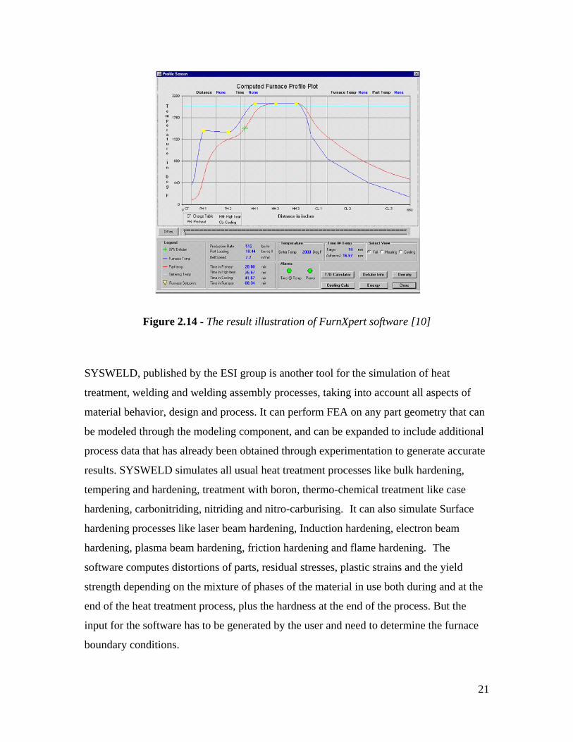
2.14 - The result illustration of FurnXpert software .................................................... 21
3.1 - Key components of a process heating system ................................................ 23
3.2 - Flowchart for temperature calculation of loaded furnace .................................. 25
3.3 - Schematic of a heat balance in a batch furnace. .............................................. 27

vii
3.4 - Schematic of a heat balance in a continuous furnace ..................................... 31
3.5 - Factors that affect the furnace temperature ..................................................... 36
3.6 - Loads in a heat treating furnace ...................................................................... 36
3.7 - The factors affecting the workpiece temperature ............................................. 37
3.8 – The equivalent workpiece ............................................................................... 39
3.9 - Schematic of the Temperature controller in a radiant tube type furnace ........ 42
3.10 - On/Off & Proportional type controllers commonly used in furnaces ............... 43
3.11 - Control feedback loop of PID control ............................................................... 45
5.1a - The thermal gradients inside a Continuous Pusher Furnace, experimental
data from continuous datapak with 6 thermocouples. .................................... 55
5.1b - The thermal profile of the CHT calculated and measured workpiece
temperature at 6 different locations in a Continuous Furnace ....................... 57
5.2 - Pusher type Continuous Furnace Model ............................................................ 58
5.3 - Door open/ Push sequence in a Continuous Furnace Model ........................... 60
5.4 - Empirical data used by a furnace manufacturer based on experiments and
experience to predict the loss of atmosphere during the door operation in a
continuous furnace ............................................................................................ 61
5.5 - The pressure in two different final zones in a Continuous Pusher Furnace ....... 62
5.6 - The pressure variations as a function of different door operations events
Holding Chamber (left) & Quench Chamber (right) .......................................... 63
5.7 - The door open schedule based on the furnace layout represented in the
time domain ....................................................................................................... 64
5.8 - The screen shot of the furnace thermal profile computed by CHT-c/f
software using the improved furnace model ..................................................... 66
5.9 - The comparison of the furnace thermal profile computed using improved
furnace model and measurement results. ........................................................ 67

viii
5.10 - The thermal gradients inside a batch type heat treating furnace .................... 69
5.11 - Furnace temperature gradients and gradient variations in a fully loaded
furnace over a period of 40 minutes in a Continuous Pusher type.
Carburizing Furnace with a push cycle time of 16 minutes. ............................ 70
5.12a - Experimental setup showing the datapak and thermocouple locations
inside the Pusher Furnace. .......................................................................... 72
5.12b - The thermal gradients inside a Continuous Pusher Furnace, experimental
data from continuous datapak with 6 thermocouples. .................................. 72
5.13 - Temperature gradient between the set point temperature and the work
area (center of furnace) at 3 different zones and locations in a Rotary type
Continuous Furnace ......................................................................................... 73
5.14 - Different burner patterns / schemes commonly used in the Pusher Type
Continuous Furnaces ....................................................................................... 75
5.15 - Thermal gradients measured at different locations in a Pusher type
Continuous Furnace with different zones marked. .......................................... 76
5.16 – The top view of boost zone with thermocouple locations and the
corresponding shim port locations for the data gathered. ............................ 77
5.17a – The measured temperature gradient pattern inside furnace – Holding
Chamber (Burner layout – I) ......................................................................... 78
5.17b – The measured temperature gradient pattern inside furnace (Burner
layout – II) .................................................................................................... 78
5.17c – The measured temperature gradient pattern inside furnace (Burner
layout –III) .................................................................................................... 79
5.18 – The gradient generated across the entire furnace using the static
experiments .................................................................................................... 79
5.19 - Calculation domain of the represented in the space domain and

ix
the location of i,j,k and zone in a Continues Pusher Furnace. ....................... 80
5.20 - Experimental setup to determine .................................................................. 81
5.21 - Trilinear interpolation scheme to populate the thermal gradients from the
experimental data ........................................................................................... 81
5.22 - Plot of workspace inside the furnace showing locations of the 6 points
measured using the experiments and 3 interpolated points (P3, P4 & P5) .... 82
5.23(a) - Interpolated at point P3 ............................................................................... 83
5.23(b) - Interpolated at point P4 ............................................................................... 83
5.23(c) - Interpolated at point P5 ............................................................................... 83
5.23 - Plots of calculated at points P3, P4 & P5 (refer Fig.5.22 for locations) .......... 83
5.24 - Comparison of the measured and improved CHT model calculated results
in a Pusher type Continuous Furnace. (Top figure - calculated near top of
the load, Bottom figure- calculated near bottom of load) ............................... 84
5.25 - Spalled and corroded furnace refractory walls ................................................. 87
6.1 - Heat distribution and balance in the furnace .................................................... 93
6.2 - Error of predicted furnace temperature (Illustration) ....................................... 95
6.3 - Strategy logic of KDD furnace model solution ................................................. 97
6.4 - Neural Network based calibration furnace model ............................................ 99
6.5 - Two layer feed forward neural network .......................................................... 100
6.6 - CHT-bf Temperature prediction with KDD model .......................................... 102
6.7 - Arrangement of workpieces in the basket and thermocouple placements ..... 103
6.8 - Comparison of CHT-bf & KDD Temperature prediction with measured
results............................................................................................................ 104
6.9 - Classification Illustration of loads with same As ............................................ 106

x
LIST OF TABLES
3.1 - Energy terms and their definitions ............................................................... 26
3.2 - Heat loss for different furnace walls construction (Btu/hr-ft2) .................. 29
3.3 - Combustion properties of typical commercial fuel gases .......................... 30
4.1 - List of case studies in different furnaces and locations ............................. 49

1
CHAPTER - 1 Introduction
Heat treating is the controlled heating and cooling of a material to achieve certain
mechanical properties, such as hardness, strength, flexibility, and the reduction of
residual stresses. Many heat treating processes require the precise control of temperature
over the heating cycle. Heat treating is used extensively in metals production, and in the
tempering and annealing of glass and ceramics products. Typically, the energy used for
process heating accounts for 2% to 15% of the total production cost. The US industrial
sector consumes 32.6 quadrillion Btu per year, over 1/3 of the total energy use in the US
with a value of $100 billion. Of that amount, 60% is consumed in fossil-fired systems
such as furnaces, boilers, and lehrs, with varying energy losses. Thermal efficiencies can
range from over 90% for condensing boilers to under 10% for small, batch operated, high
temperature furnaces like heat treat furnaces [1]. In order to improve the energy
efficiency and optimize the load throughput, it’s vital to have numerical modeling
capability to accurately simulate the heat treatment processes. Currently there are plenty
of commercial solutions for modeling the heat transfer and material properties for a
single workpiece but none of them have a furnace model for simulating the thermal
profile of the entire load. A comprehensive furnace model for different kinds of furnaces
is crucial to accurately simulate the temperature of the load.
1.1 Objectives and scope of study The objective of this work is to develop a comprehensive furnace model by
improving the current Computerized Heat Treatment Planning System (CHT) based
furnace model. The research methodology was based on both experimental work and
theoretical developments including modeling different types of heat treat furnaces. More
than 40 experimental validations through case studies using the current CHT model were
conducted in 11 manufacturing locations to identify the specific problems in the current
model. From the experimental data and knowledge from the experiments several
improvements to the current furnace model are implemented and a new furnace model

2
based on Knowledge Data Discovery (KDD) technique is also developed and validated.
A furnace tuning and calibration procedure is developed based on a virtual load design.
The main improvements include modeling thermal gradients present inside the
furnace and accounting for heat loss arising due to the furnace door openings during
loading and unloading of the furnaces. Also a virtual load is design procedure is
developed for different loads and the reverse calculation for determining the furnace
emissivity that accounts the wear and tear. Several constants are added to the current heat
balance equation and they are determined using the experimental data and neural
network. This KDD based model is used to optimize the load pattern using maximum
entropy.
It is possible to accurately predict the thermal profile of the load inside a furnace
using the improved furnace model. The new model enables us to improve the furnace
efficiency by maximizing the load throughputs and save energy by accurately predicting
the cycle time. The new model takes into account all the real time furnace parameters
determined from the experimental data and accounts for some of the complex gradients
and heating patterns that exist inside the furnace that is difficult to model. Based on
experimental results the model is trained using neural network and the new improved
KDD based model is validated with case studies at different production facilities.

3
1.2 Dissertation organization This dissertation is organized into six parts:
Part I - (Chapter 1 – 2) Introduction and Review
Chapter 1. Introduction (this chapter). Introduces the background, specific problem,
objectives, solution and results of this research.
Chapter 2. Literature Review. Gives a review of earlier studies related to the furnace
models and softwares.
Part II - (Chapter 3) Current Furnace Model & (Chapter 4 & Appendix - A) Furnace
Model Analysis
The current model furnace model for both batch and continuous furnaces are studied in
detail. It studies the different heat terms in the furnace model and how they are
calculated. A detailed analysis is conducted through experimental case studies at different
industries (Appendix –A) The furnace model analysis is done to identify the areas for
improvement to the current model.
Part IV- (Chapter 5) Furnace model improvements
The furnace model improvements are divided into three sub chapters: Door open model –
describes the addition of the heat loss term to the CHT model, Thermal Gradients –
describes the approach the model to incorporate the thermal gradients present in the
model. Virtual load – describes the virtual load calibration procedure.
Part V (Chapter 6) Knowledge Data Discovery (KDD) based furnace model
A new intelligent furnace model based on Knowledge data discovery is proposed and the
model is validated by using industrial case studies
Part VI - (Chapter 7) Summary
The different improvements to the current model and their advantages and limitations are
studied in detail.
Appendix A. Analysis of experimental case studies
4
CHAPTER – 2 Background and literature review This chapter discusses the various researches done in modeling the heat treat
furnaces and different software models available for performing the heat treat thermal
simulation and their features and limitations.
2.1 Heat treating process overview Heat Treatment may be defined as heating and cooling operations applied to
metals and alloys in solid state so as to obtain the desired properties. Heat treatment is
sometimes done inadvertently due to manufacturing processes that either heat or cool the
metal such as welding or forming. Heat treatment is often associated with increasing the
strength of material, but it can also be used to refine the grain size, relieve internal stress,
to improve machinability and formability and to restore ductility after a cold working
process. Some of the objectives of heat treatment are summarized as follows:
• Improvement in ductility
• Relieving internal stresses
• Refinement of grain size
• Increasing hardness or tensile strength
• Improvement in machinability
• Alteration in magnetic properties
• Modification of electrical conductivity
• Improvement in toughness

5
Figure 2.1 - Energy Source Breakdown for Key Industrial Process
Heating Applications [2]
The energy source for the heat treating industry is more than 80% from gas. Fig.
2.1 illustrates how fuels are used in several process heating applications. The costs of
different fuel types can vary widely, which has a significant impact on the payback
period of efficiency improvement projects.
A heated workpiece in a heat-treating furnace will undergo a given thermal schedule,
typically, a heating ⎯ soaking ⎯ cooling cycle. (Fig. 2.2)
Figure 2.2 – A typical heat treatment cycle for a typical carburizing process with a
reheat cycle [3]

6
2.1.1 Basic requirements of heat treatment process The main requirement of the heat treatment process is the accurate control of the
temperature profile. And also soaking/holding at specified temperature for obtaining
uniform cross section temperature across load and workpiece is another basic
requirement of the heat treatment process. In processes like carburizing once the load
reaches the soaking temperature the enriching hydrocarbon gas is added to the furnace
and the load is held at the carburizing temperature for the carbon diffusion to occur until
the required case depth is achieved. And the cooling cycle is determined by the required
microstructure desired. And the cooling can be either liquid or gas cooling depending on
the furnace.
2.1.2 Basic requirements of furnaces The main requirement of the furnaces in the heat treatment process is to provide
the necessary heat input for the load/workpiece. The furnace also requires a control
system to control the temperature in the furnace accurately. Also a uniform temperature
distribution is desired inside the furnace. Apart from the temperature controller there are
also several atmosphere controllers and material handling controllers required based on
the type of furnaces.
2.1.3 Heat treatment processes There are several different types of heat treatment processes. By controlling the soak
temperature and the cool down rate of the steel, we can determine the process to be
accomplished. Those processes include,
• Annealing
• Normalizing
• Stress relieving
• Hardening
• Tempering

7
Annealing
Annealing is the process of heating the steel to a particular temperature in the austenite
region and cooling down the steel very slowly. There are many derivatives of the
annealing process, but generally the process is a slow cool process.
Another derivative of the annealing process is known as sub-critical anneal. This process
involves soaking at a temperature below the lower transformation line, in the region of
1,200F to 1,300F, until the steel has equalized across its cross-section in temperature,
followed by a slow cool. Slow cooling can mean a cooling rate between 5F per hour up to
50F per hour.
Normalizing
Normalizing is a process that makes the grain size normal. This process is usually carried
out after forging, extrusion, drawing or heavy bending operations. When steel is heated to
elevated temperatures to complete the above operations, the grain of the steel will grow.
In other words, the steel experiences a phenomenon called "grain growth." This leaves
the steel with a very coarse and erratic grain structure. Furthermore, when the steel is
mechanically deformed by the aforementioned operations, the grain becomes elongated.
There are mechanical property changes that take place as a result of normalizing -
inasmuch as the normalized steel is soft, but not as soft as a fully annealed steel. Its grain
structure is not as coarse as an annealed steel, simply because the cooling rate is faster
than that of annealing. Usually the steel is cooled in still air and free from air drafts. The
process temperature is virtually the same as for annealing, but the results are different due
to the cooling rate.
Stress relieving
Stress relieving is an intermediate heat treatment procedure to reduce induced residual
stresses as a result of machining, fabrication and welding. The application of heat to the
steel during its machining or fabrication will assist in removing residual stresses that will,

8
unless addressed during the manufacturing by stress relieving, manifest themselves at the
final heat treatment procedure.
It is a relatively low temperature operation that is done in the ferrite region, which means
that there is no phase change in the steel, only the reduction of residual stresses. The
temperature region is usually between 800F to 1,300F. However, the higher that one goes
in temperature, the greater the risk of surface oxidation there is. It is generally better to
keep to the lower temperatures, particularly if the steel is a "pre-hard" steel. The hardness
will be reduced if the stress relieve temperature exceeds the tempering temperature of the
steel.
2.2 Types of furnaces
The furnaces used in the heat treating process can be classified in several different
ways. The most popular classification method is shown in Fig. 2.3.
Figure 2.3 – Furnace Classification
2.2.1 Classification based on heating method
One of the popular methods of classifying the furnaces is based upon the heating
or energy input method. And it can be divided into combustion based heating and electric
heating methods.
Combustion-based (Fuel-based) Process Heating

9
Heat is generated by the combustion of solid, liquid, or gaseous fuels, and transferred
either directly or indirectly to the material. Common
fuel types are fossil fuels (e.g. oil, natural gas, coal) The combustion gases can be either
in contact with the material (direct heating), or be confined and thus be separated from
the material (indirect heating; e.g., radiant burner tube, radiant panel, muffle).
Electric process heating (Electrotechnologies)
Electric currents or electromagnetic fields are used to heat the material. Direct heating
methods generate heat within the work piece, by either (1) passing an electrical current
through the material, (2) inducing an electrical current (“eddy current”) into the material,
or (3) by exciting atoms/molecules within the material with electromagnetic radiation
(e.g. microwave). Indirect heating methods use one of these three methods to heat a
heating element or susceptor, and transfer the heat either by conduction, convection,
radiation or a combination of these to the work piece.
2.2.2 Classification based on mode of operation
Another classification of the furnaces is based on the mode of operation. The
classification is either a batch type operation or a continuous operation.
Batch furnaces
The basic batch furnace normally consists of an insulated chamber with an
external reinforced steel shell, a heating system for the chamber, and one or more access
doors to the heated chamber. Standard batch furnaces such as box, bell, elevator, car-
bottom, and pit types are most commonly used when a wide variety of heat-hold-cool
temperature cycles are required. Batch furnaces are normally used to heat treat low
volumes of parts (in terms of weight per hour). Batch furnaces are also used to carburize
parts that require heavy case depths and long cycle times. These furnaces are either
electrically heated or gas/oil fired. The gas/oil fired furnaces can further be classified as
direct fired and in-direct fired (radiant tube burners)

10
Figure 2.4 - A schematic of Batch–Integral furnace [5]
Vacuum furnaces (Type of batch furnace)
In most heat-treating processes, when materials are heated, they react with atmospheric
gases. If this reaction is undesirable, the work must be heated in the presence of some gas
or gas mixture other than normal air. This is done in normal atmosphere furnace
processing. The gas or gas mixture may be varied to cause desirable reactions with the
material being processed or it may be adjusted so that no reactions occur. At different
temperatures, different reactions may occur with the work and furnace atmosphere. In
most atmosphere furnaces it is not possible to change the atmosphere composition rapidly
enough for optimum reactions or to control the atmosphere composition with the degree
of precision required for some heat-treating processes. Vacuum furnaces allow gas
changes to be made quite rapidly because they contain gases of low weight. Vacuum
furnace technology removes most of the components associated with normal atmospheric
air before and during the heating of the work. Fig. 2.2 shows a typical vacuum
carburizing cycle with time and pressure vs time plot.

11
Continuous furnaces
Continuous furnaces consist of the same basic components as batch furnaces: an
insulated chamber, heating system, and access doors. In continuous furnaces, however,
the furnaces operate in uninterrupted cycles as the workpieces move through them.
Consequently, continuous furnaces are readily adaptable to automation and thus are
generally used for high-volume work. Another advantage of continuous furnaces is the
precise repetition of time-temperature cycles, which are a function of the rate of travel
through the various furnace zones. A multi chamber pusher-type continuous carburizing
furnace system is widely used in industry where the heating, carburizing, and diffusion
portions of the cycle are separated.
Figure 2.5 - Pusher-type and rotary-hearth heat-treat system [5]
2.2.3 Classification based on material handling system The selection of the material handling system depends on the properties of the material,
the heating method employed, the preferred mode of operation (continuous, batch) and
the type of energy used. An important characteristic of process heating equipment is how
the load is moved in, handled, and moved out of the system. Several important types of
material handling systems are,
• Conveyor, Belts, Buckets, Rollers
• Rotary Hearth Furnaces

12
• Walking Beam Furnaces
• Pusher Type Furnaces
• Car Bottom Furnaces
• Continuous Strip Furnaces
2.3 Furnace heat input 2.3.1 Indirect fired (Radiant-tube) furnaces
Figure 2.6 - Schematic of the indirect-fired section of the
Inland Steel annealing furnace [8]
‘A Thermal System Model for a Radiant-Tube Continuous Reheating Furnace’
discusses about a thermal system mathematical model developed for a gas-fired radiant-
tube continuous reheating furnace (Fig. 2.6). The mathematical model of the furnace
integrates submodels for combustion and heat transfer within the radiant tube with
models for the furnace enclosure. The transport processes occurring in the radiant tube
are treated using a one-dimensional scheme, and the radiation exchange between the load,
the radiant-tube surfaces, and the furnace refractories are analyzed using the radiosity

13
method. The continuous furnace operation is simulated under steady-state conditions. The
scope and flexibility of the model are assessed by performing parametric studies using
furnace geometry, material properties, and operating conditions as input parameters in the
model and predicting the thermal performance of the furnace. The various parameters
studied include the effects of load and refractory emissivities (Fig. 2.7), load velocities,
properties of the stock material [8].
Figure 2.7 - Variations in the furnace thermal efficiencies with load and refractory
emissivities (left) & Variations in the load and roof surface
temperatures with distance for varying load emissivities (right)[8]
Another study is conducted to access the different types of radiant tube designs. Fig 2.8
which shows the variations in the load surface temperature for the same net fuel firing
rate in the radiant tubes, indicates that the load surface temperatures are the highest for
the W-type tube design, followed by the U-type and then the straight-through tubes. The
lower load surface temperatures for the straight-through tubes in the furnace is due to the
incomplete burning of fuel in the radiant tubes. A considerable amount of energy is lost
in the form of unburned fuel at the exhaust of the straight-through tube. However, in the
U-type and W-type tubes, further burning of the unburned fuel from the first branch takes
place, resulting in a higher average tube wall temperature in the successive branches of
the tube [8].

14
Figure 2.8 - Variations in the load and crown surface temperatures
with distance for different radiant-tube designs in the furnace[8]
2.3.2 Direct fired furnaces ‘The Development, Verification, and Application of a Steady-State Thermal Model for
the Pusher-Type Reheat Furnace’ outlines the development of a steady-state thermal
model for the pusher-type steel reheating furnace. (Fig.2.9) Commonly encountered
energy consumption are analyzed. The objective of the work is to provide a means by
problems with this furnace type like skidmark generation, scale formation, and high
which furnace users might assess the effectiveness of changes to current operating
practice, proposed furnace modifications, or new furnace designs in controlling these
difficulties. The model is verified using data obtained in plant trials on several 32-m
furnace reheating slabs, and model predictions for steel temperatures at six locations

15
within the steel are compared with the experimental results. The inclusion of a hearth in
Figure 2.9 - A typical pusher-type direct fired furnace: (a) longitudinal section,
(b) transverse section [9].
the furnace soak zone was found to impose the least severe skidmark on the product,
reducing the temperature variation over the bottom face from the level of 130 ~ incurred
by the best of the soak zone skid configurations examined, to the level of 85 ~ The results
suggest that, in the absence of a hearth section, the use of a well-insulated,
cold-rider skid system over the majority of the furnace length, followed by a single offset
of all skids occurring at the transition to a short section of hot-rider skids near the furnace
discharge, is sufficient to suppress the final skidmark to a level very close to the
minimum achievable with that particular skid design. When assessed on the basis of
minimizing both the final skidmark and the energy loss to the skid system, this
configuration was found to be the best of the skid layouts examined

16
Figure 2.10 – (a) A comparison of model predictions for steel temperature
and plant data at between-skid thermocouple locations.
(b) A comparison of model predictions for steel temperature and plant data
at over-skid thermocouple locations[9].
‘Modeling and Parametric Studies of Heat Transfer in a Direct-Fired Continuous
Reheating Furnace’ – is a mathematical system model of a direct-fired continuous
reheating furnace. The furnace is modeled as several well-stirred gas zones with one-
dimensional (l-D) heat conduction in the refractory walls and two-dimensional heat
transfer in the load. The convective heat-transfer rate to the load and refractory surfaces
are calculated using existing correlations from the literature. Radiative heat exchange
within the furnace is calculated using Hottel's zone method by considering the radiant
energy exchange between the load, the combustion gases, and the refractories. The
nongray characteristics of the combustion gases are considered by using a four-gray gas
model to treat the mixture as a radiatively participating medium. The parametric
investigations included in this paper study the effects of the load and refractory
emissivities and the height of the combustion space on the thermal performance of the
furnace.

17
2.4 Furnace control Thermal imaging control of furnaces and combustors developed by Gas
Technology Institute [6]. The objective of this project is to demonstrate and bring to
commercial readiness a near infrared thermal imaging control system for high
temperature furnaces and combustors.
The concept used in this project is to provide improved control to high temperature
furnaces using a near-IR thermal imaging control system. Initial stages of the Thermal
Imaging sensor hardware development were conducted by testing on a laboratory electric
furnace. The complete system was then tested on a GTI heat treat furnace. A state-of-the-
art control system was installed and accepted input for control from the thermal imaging
system.
Figure 2.11 – Comparison of the thermocouples with the thermal imaging system and the
thermal gradient inside the box type furnace [6]
The project strategy is to input the thermal imaging system data into a set of control
system algorithms that would give secondary control instructions to burners (air-fuel
ratios, etc.) for tuning control.

18
2.5 The need to model furnaces A commonly overlooked factor in energy efficiency is scheduling and loading of
the furnace. “Loading” refers to the amount of material processed through the furnace in
a given period of time. It can have a significant effect on the furnace's energy
consumption when measured as energy used per unit of production (Btu/lb). Certain
furnace losses (wall, storage, conveyor and radiation) are essentially constant regardless
of production volume; therefore, at reduced throughputs, each unit of production has to
carry a higher burden of these fixed losses. Flue gas losses, on the other hand, are
variable and tend to increase gradually with production volume. If the furnace is pushed
past its design rating, flue gas losses increase more rapidly, because the furnace must be
operated at a higher temperature than normal to keep up with production. Total energy
consumption per unit of production will follow the curve in Fig. 2.12, which shows the
lowest at 100% of furnace capacity and progressively higher the farther throughputs
deviate from 100%. Furnace efficiency varies inversely with the total energy
consumption. The lesson here is that furnace operating schedules and load sizes should be
selected to keep the furnace operating as near to 100% capacity as possible. Idle and
partially loaded furnaces are less efficient
Figure 2.12 - Impact of production rate on energy consumption per unit of production
[2].

19
In order to achieve maximum efficiency it is required to design the furnace part load to
the maximum furnace capacity. A numerical tool with a furnace model helps to achieve
this goal. Also another important quality metric in the heat treatment processes is soak
time (amount of time a load stays at a given temperature) A furnace model with
workpiece thermal profile prediction can accurately predict the time required to reach the
process temperature and the soak time. So the process can be accurately designed
eliminating guesses and removing conservative recipes.
2.6 Current research
The current research to model the heat treatment process is focused mostly on a single
part model using the commercially available FEM software tools. The topics discussed in
chapters 2.3.1 and 2.3.2 are the research conducted by E.S Chapman et al and it focuses
on using the FEM method with temperature boundary conditions [9].
Limitations
The major limitations of the single part model and the FEM based model are the
determination of the temperature boundary condition. The temperature boundary
condition is an important input for the model and the results are dependent on the
accuracy of the boundary conditions. Every furnace is unique in the heat treatment
industry so it’s difficult to determine the boundary condition without a comprehensive
furnace model. Currently none of the research is focused on the furnace model. Also
FEM based approach is a computation intensive and consumes several hours for
calculating results.
2.7 Current software tools
Process Heating Assessment and Survey Tool (PHAST) – is a software tool developed at
DOE for identifying methods to improve thermal efficiency of heating equipment. This
tool helps industrial users survey process heating equipment that consumes fuel, steam, or
electricity, and identifies the most energy-intensive equipment. Use the tool to compare

20
performance of equipment under various operating conditions and test "what-if"
scenarios. PHAST constructs a detailed heat balance for selected pieces of process heat-
ing equipment. The process considers all areas of the equipment in which energy is used,
lost, or wasted. Results of the heat balance pinpoint areas of the equipment in which
energy is wasted or used unproductively.
FurnXpert program is developed to optimize furnace design and operation. The program
mainly focuses on the heat balance of the furnace. The load pattern is just aligned load
pattern with one layer and it cannot deal with the condition of workpieces loaded in the
fixtures. While, in this condition the workpieces inside the fixture are heated by adjacent
workpieces, not directly by furnace. Figure 2.13 shows an interface of load pattern
specifications in FurnXpert. The result curves are shown in Figure 2.14
Figure 2.13 - The load pattern for continuous belt in FurnXpert software [10]
21
Figure 2.14 - The result illustration of FurnXpert software [10]
SYSWELD, published by the ESI group is another tool for the simulation of heat
treatment, welding and welding assembly processes, taking into account all aspects of
material behavior, design and process. It can perform FEA on any part geometry that can
be modeled through the modeling component, and can be expanded to include additional
process data that has already been obtained through experimentation to generate accurate
results. SYSWELD simulates all usual heat treatment processes like bulk hardening,
tempering and hardening, treatment with boron, thermo-chemical treatment like case
hardening, carbonitriding, nitriding and nitro-carburising. It can also simulate Surface
hardening processes like laser beam hardening, Induction hardening, electron beam
hardening, plasma beam hardening, friction hardening and flame hardening. The
software computes distortions of parts, residual stresses, plastic strains and the yield
strength depending on the mixture of phases of the material in use both during and at the
end of the heat treatment process, plus the hardness at the end of the process. But the
input for the software has to be generated by the user and need to determine the furnace
boundary conditions.

22
2.8 Summary
Heat treatment is an important manufacturing process. The furnace is key element
in the heat treat process. The heat treat process variations can often be attributed to
temperature variations in the process. So a tight control of temperature during the process
is key to achieve minimum part variations during heat treatment. Also the modeling study
is very limited. The current research is focused mostly on Finite Element Analysis based
approach. And all the tools predict the microstructure and material properties for a given
workpiece. The key input for these tools is the thermal profile of the heat treat process
and there is no comprehensive solution currently available.

23
CHAPTER – 3 CHT furnace model 3.1 Overview of current Computerized Heat Treatment (CHT) furnace model Common to all process heating systems is the transfer of energy to the material to
be heat treated. Direct heating methods generate heat within the material itself
(microwave, induction, controlled exothermic reaction), whereas indirect methods
transfer energy from a heat source to the material by conduction, convection, radiation, or
a combination of these functions. In most processes, an enclosure is needed to isolate the
heating process and the environment from each other. Functions of the enclosure include,
but are not restricted to, the containment of radiation (microwave, infrared), the
confinement of combustion gases and volatiles, the containment of the material itself, the
control of the atmosphere surrounding the material, and combinations thereof. Common
industrial heat treat process heating systems fall in one of the following categories:
• Combustion-based process heating systems
• Electric process heating systems
Figure 3.1 - Key components of a process heating system [15]

24
Temperature control is one of the most important aspects in heat treatment
process. Heat treatment temperature mainly refers to soaking temperature and time. The
soak temperature and time significantly affect the material properties of parts. The
furnace productivity and efficiency are maximized by aggressive part load design and
optimum thermal schedules.
Currently in the industry part load design is determined based on experience and
empirical rules. With the advent of several heat transfer simulation tools it is now
possible to simulate heat transfer of the workpieces in a furnace. Although there are a lot
of commercial FEA tools available for simulation they all require a boundary condition
for the simulation. Determining the boundary condition is difficult as it involves a
complex furnace model.
The CHT software was developed for simulating the thermal profiles of the parts
inside a furnace based on a hybrid FDM and empirical solution. The core of the software
is the furnace model that was developed based on several empirical equations determined
through experiments and knowledge and expertise derived from the furnace
manufacturers. To accurately calculate the part temperature it is important to calculate the
furnace temperature and heat balance in the furnace. Figure 3.2 shows the flow chart for
the calculation of furnace temperature using the CHT furnace model.
The CHT furnace model can be divided into furnace energy balance model, heat
transfer model and furnace control model.

25
INPUT
PREPROCESSING
MAIN MODULES
Part properties calculation: • Geometry and sizes • Surface area(A) and Volume(V) • Equival. thickness (t_eff) • Weight (M_wp)
Furnace parameters calc/setting: • Surface area (A_ext) • Alloys weight (V, ρ, M_Alloy) • Insulation weight (M_insu) • Cooling air folw capacity (Flow_clg)
Thermal schedule designTime –temperature table & profile
Part load design • Parts quantity and weight
• Parts arrangement in furnace
Initial/boundary condition setting • Furnace temperature (T_fce) • Part temperature (T_ld) • Medium temperature (T_air)
Calculation parameters setting • Calculation intervals (δt) • Stefan Boltzmann constant (σ) • Emissivity of workpiece (ε) • Convection film coefficient (h)
Part temperature calculation: • Specific heat calculation (cp) • Part Average Temp calculation
Furnace temperature calculation • Furnace heat storage (q_storage) • Furnace average temperature calculation (T_fce)
Furnace energy calculation • Effective heat input (q_ht) • Heat loss (q_loss) • Gross heat to loads (q_ld) • Fan heat calculation (q_fan) • Furnace cooling (q_cl)
Furnace control: • PI control model • PI parameters setting (GP, GI )
OUPUT (Thermal Profile)
Convection heat transfer
Coefficient (h) • Heat flow calculation
Radiation heat transfer • View factor calculation • Heat flow calculation
Figure 3.2 - Flowchart for temperature calculation of loaded furnace
Workpiece DB
Materials DB
Furnace DB
H.T. Spec. DB / Material DB
FurnaceDB

26
3.2 Furnace energy balance model Heat storage is calculated according to the energy balance,
(Heat storage) ∼ Function of [(Available heat), (Heat to load),(Wall losses), (Radiation losses)]
(Available Heat) ∼ Function of (Gross input)
Table 3.1 - Energy terms and their definitions[11]
Energy Items Definitions
Gross Input The total amount of heat used by the furnace.
Available Heat Heat that is available to the furnace and its workload, including workpiece, furnace structural components, accessories, and heat losses due to furnace itself.
Heat to Load Heat that ultimately reaches the product in the furnace.
Wall Losses Heat conducted out through the furnace walls, roof and floor due to the temperature difference between inside and outside.
Radiation Losses Heat lost from the furnace as radiant energy escaping through openings in walls, doors, etc.
Heat Storage Heat absorbed by the insulation and structural components of the furnace to raise them to operating temperature.
q_storage = q_ht - q_ld - q_loss - q_air + q_fan (3.1)
where q_ht is effective heat input; q_loss is heat loss; q_ld is the heat to the workpieces;
q_air is heat absorbed by atmosphere; and q_fan is the heat input effect created due to the
increase in convection by fan. (Fig. 3.3)

27
Figure 3.3 – Schematic of a heat balance in a batch furnace.
3.2.1 Energy terms calculation (Indirect gas-fired batch furnace)
Effective heat input (q_ht) :
q_ht = Htg · AHC · q_conn (3.2)
where Htg is an adjust coefficient for heat input. The calculation will be given in the next
section.
AHC is the corrected coefficient to the gross heat input
AHC = AH1 + AH2 + AH3 (3.3)
where, the values AH,AH2 & AH3 are based on the experimental data:

28
Heat to load (q_ld):
The heat to load, is mainly subjected to the hybrid convection and radiation heat transfer.
It can be calculated using the following equation:
( ) ( )4_
4___
___ ldfceldfce
ldldld TTTTh
tddT
kq −⋅⋅+−⋅=⎟⎟⎠
⎞⎜⎜⎝
⎛⋅= εσ (3.4)
Heat loss (q_loss):
Heat loss depends on the design factor for the heat loss of furnace and the surface area of
furnace. Following is an empirical equation:
q_loss = DF·( Q_loss_wall + Q_loss_rad) (3.5)
where, DF is the design factor, and A_ext is the surface area of furnace.
Furnace wall losses:
Q_loss_wall = A_fce × f (T_fce) (3.6) where A_fce is furnace wall area (inside); f (T_fce) is a function for heat loss, in Btu/ft2-hr.
Typical heat loss data are tabulated in Table 3.2
Radiation losses:
( )44___ ambgasopenradloss TTAQ −⋅⋅= σ (3.7)
where, Q_loss_rad is the radiation losses, A_open is the opening area, Tgas is the temperature
of furnace gas, Tamb is the temperature of ambient outside furnace, σ is Stefan-Boltzmann
constant.

29
Table 3.2 - Heat loss for different furnace walls construction (Btu/hr-ft2)[11]
Fan heat input effect (q_fan):
It is calculated based on an empirical equation:
⎟⎟⎠
⎞⎜⎜⎝
⎛
+⋅=
fcefanfan T
HPq_
__ 460520 (3.8)
where, HP_fan is the horsepower of re-circulating fan.
Heat absorbed by air (q_air)
q_air = Clg ⋅ Flow_air ⋅ ρ ⋅ cp ⋅ (T_fce – T_air) (3.9)
Wall Construction
Hot Face Temperature, °F 1000 1200 1400 1600 1800 2000 2200 2400
9" Hard Firebrick 550 705 862 1030 1200 1375 1570 17689" Hard Firebrick + 4.5" 2300° Insulating F.B. 130 168 228 251 296 341 390 447
9" Hard Firebrick + 4.5" 2000° Insulating F.B. +2" Block Insulation
111 128 155 185 209 244 282 325
4.5" 2000° Insulating F.B. 185 237 300 365 440 521 - - 9" 2000° Insulating F.B. 95 124 159 189 225 266 9" 2800° Insulating F.B. 142 178 218 264 312 362 416 4749" 2800° Insulating F.B. + 4.5" 2000° Insulating F.B. 115 140 167 197 232 272 307 347
9" 2800° Insulating F.B. + 4.5" 2000° Insulating F.B. + 2" Block Insulation
71 91 112 134 154 184 204 230
9" 2800° Insulating F.B. + 3" Block Insulation 114 142 172 201 232 264 298 333 8" Ceramic Fiber – Stacked Strips, 8 #/cu ft Density 27 45 64 86 114 146 178 216 10" Ceramic Fiber – Stacked Strips, 8 #/cu ft Density 16 35 54 76 94 120 142 172 12" Ceramic Fiber – Stacked Strips, 8 #/cu ft Density 13 27 43 60 79 98 118 143 9" Hard Firebrick + 3" Ceramic Fiber Veneer, 8 #/cu ft Density 177 240 309 383 463 642 721 800
9" 2800° Insulating F.B. + 3" Ceramic Fiber Veneer, 8 #/cu ft Density
102 125 151 183 227 274 325 408

30
where Clg is the PID control variable,
Flow_air is the airflow heated by the fuel gas and it equals to
( )air
Grossair xsR
hvQ
Flow __
_ 1+⋅⋅= (3.10)
where hv is the gross heating value of commercial fuel gases, as listed in Table 3.3; R is
the stoichiometric air/gas ratio, listed in Table 3.3; Q-gross is the gross heat input; xs-air is
the combustion access air; ρ is air density; cp is the air specific heat; T_fce is the furnace
temperature; and T_air is the air temperature before mixed enter furnace.
Table 3.3 - Combustion properties of typical commercial fuel gases[11]
Gas type Heating value(Btu/ft3)
Heating value(Btu/lb)
Air/Gas Ratio (ft3 air/ft3 gas)
Air/Gas Ratio(lb air/lb gas)
Acetylene 1498 21,569 11.91 13.26 Hydrogen 325 61,084 2.38 33.79 Butane (natural gas) 3225 21,640 30.47 15.63 Butylene (Butene) 3077 20,780 28.59 14.77 Carbon Monoxide 323 4368 3.38 2.46 Carburetted Water Gas 550 11,440 4.60 7.36 Ethane 1783 22,198 16.68 15.98 Methane 1011 23,811 9.53 17.23 Natural (Birmingham, AL) 1002 21,844 9.41 15.68 Natural (Pittsburgh, PA) 1129 24,161 10.58 17.31 Natural (Los Angeles, CA) 1073 20,065 10.05 14.26 Natural (Kansas City, MO) 974 20,259 9.31 14.59 Natural (Groningen, Netherlands) 941 19,599 8.41 13.45 Propane (natural gas) 2572 21,500 23.82 15.37 Propylene (Propene) 2322 20,990 21.44 14.77
3.2.2 Heat balance in continuous furnace
The calculation deals with static condition. Therefore the heat balance is dynamic. It is
assumed furnace temperature doesn’t vary to load changes. So the heat storage in the
furnace need not be calculated. (Fig 3.4) The heat terms only refer to the heat input, heat
absorption by the load and moving accessories and heat loss. The furnace structure and

31
accessories are classified into two types: moving and fixed/shaking. The moving
accessories take away heat while the fixed or shaking accessories do not take away heat.
Figure 3.4 – Schematic of a heat balance in a continuous furnace.
Heat balance in each zone:
The dynamic heat balance is
pcoolingshellpzoneplosswallpbeltpfixploadpfanpinput QQQQQQQQ __________ +++++=+
(3.11)
where,
pinputQ _ ---the heat input by furnace
pfanQ _ --- the heat input by fan
ploadQ _ ---the heat absorption by load
pfixQ _ ---the heat absorption by fixture
pbeltQ _ ---the heat absorption by belt

32
plosswallQ __ ---the heat loss from furnace wall
pzoneQ _ ---the heat transfer between zones and heat loss from the end zones
pcoolingshellQ __ ---the heat absorption by shell cooling water
From the above equation the heat input by furnace can be calculated indirectly as follows,
pfanpcoolingshellpzoneplosswallpbeltpfixploadpinput QQQQQQQQ __________ −+++++= (3.12)
It is compared with the power of the furnace to see if it exceeds the power, which means
the heat balance cannot be maintained. So the furnace temperature control system such as
PID is not considered.
The heat balance is calculated when a cycle is finished. Then the heat absorption
in each zone is calculated based on the relationship between calculation domain and zone
length. These heat terms are the functions of furnace temperature. The furnace
temperature is adjusted to maintain the heat balance. The heat input should also be
calculated directly by the connected heat input and the available heat coefficient.
Energy terms calculation
In the following equations, p refers to furnace zone number, i,j,k refers to workpiece
number, m refers to time constant. The following equations discuss the heat balance in
each zone during a time step delta t.
Heat absorbed by the load:
ploadpload CQ __ =
)()( ,,1
,,m
kjim
kjiwpi j k
TTgc −+∑∑∑ ρ
(3.13)
where ploadC _ is the ratio of load held in each zone over the calculation domain; the total
of i, j, k is for the calculation domain and not for the whole furnace zone.
33
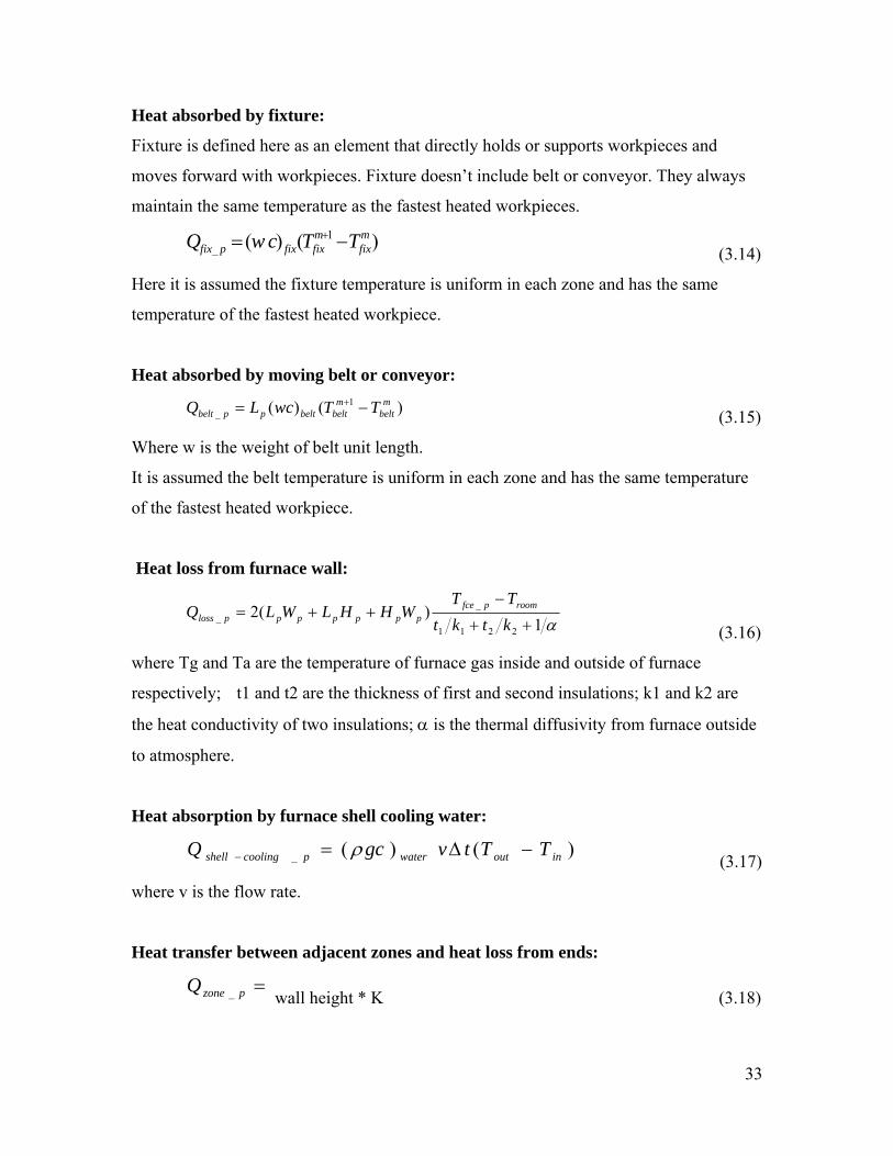
Heat absorbed by fixture:
Fixture is defined here as an element that directly holds or supports workpieces and
moves forward with workpieces. Fixture doesn’t include belt or conveyor. They always
maintain the same temperature as the fastest heated workpieces.
)()( 1_
mfix
mfixfixpfix TTcwQ −= +
(3.14)
Here it is assumed the fixture temperature is uniform in each zone and has the same
temperature of the fastest heated workpiece.
Heat absorbed by moving belt or conveyor:
)()( 1_
mbelt
mbeltbeltppbelt TTwcLQ −= +
(3.15)
Where w is the weight of belt unit length.
It is assumed the belt temperature is uniform in each zone and has the same temperature
of the fastest heated workpiece.
Heat loss from furnace wall:
α1)(2
2211
__ ++
−++=
ktktTT
WHHLWLQ roompfceppppppploss
(3.16)
where Tg and Ta are the temperature of furnace gas inside and outside of furnace
respectively; t1 and t2 are the thickness of first and second insulations; k1 and k2 are
the heat conductivity of two insulations; α is the thermal diffusivity from furnace outside
to atmosphere.
Heat absorption by furnace shell cooling water:
)()(_ inoutwaterpcoolingshell TTtvgcQ −Δ=− ρ
(3.17)
where v is the flow rate.
Heat transfer between adjacent zones and heat loss from ends:
=pzoneQ _ wall height * K (3.18)

34
K- constant. The heat transfer between heating zones can be neglected. While the heat
transfer between hot zone and cold zone, between end zones and atmosphere cannot be
neglected.
Heat release by circulation fan:
t
THPQ
fcefanpfan Δ⎟
⎟⎠
⎞⎜⎜⎝
⎛
+⋅=
__ 460
520
(3.19)
where fanHP is the power of the fan.
Heat input by the furnace:
tqKQ connAHpfce Δ⋅=_ (3.20)
Net heat input:
tqKKQ pconnpAHpPIDpnet Δ= ____ (3.21)
where pPIDK _ is the constant for PID control;AHK is the constant for combustion. For
electric furnace pAHK _ is 1. pconnq _ is the heat connected input by dialog . pPIDK _ is
calculated as follows
tTTItTTD
TPTTK pfce
mpsp
mpfcem
pfcem
span
pfcem
pspm
pPID Δ−+Δ−
+⋅−
= ∑−
)()(__
_1
____
(3.22)

35
3.3 Heat transfer model The temperature history of the loaded furnace in the heat treating cycle is a hybrid
convection/radiation heat transfer process. According to the heat transfer theory and
energy balance equation, the heat exchange of loaded furnace can be mathematically
presented in the following model:
∑= ∂
∂⋅⋅⋅=
N
i
iiistorage
TVcpq1
_ )(τ
ρ (3.24)
where N is the quantity of accessories in the furnace. For convenience, we assume that all
the accessories have the same Let time step be k and time calculation interval be δτ. The
equation can be rearranged in the time step (k+1) for the average furnace temperature.
∑=
+
⋅⋅
⋅+= N
iiii
kstoragek
fcek
fce
Vcp
qTT
1
__
1_
)(ρ
δτ (3.25)
where q_storage is the average storage of heat flux in loaded furnace; δτ is the time interval;
ρi, cpi, and Vi are the density, specific heat, and the volume of accessory i in the furnace.
These accessories include all the components involved in the heat treating process except
for the workpieces. Eq. 3.25 can be used to calculate the furnace average temperature at
time step (k+1). The equation is further grouped and rewritten as:
fce
kstoragek
fcek
fce HCQ
TT−
+ ⋅+=
δτ__
1_ (3.26)
where, Q_storage is the heat storage in heat-treating furnace; HC_fce is the heat capacity of
furnace components; k is the time step; and δτ is the time interval.
3.3.1 Factors that affect the furnace temperature calculation
The main factors affecting the furnace temperature are loads and heat storage.
Loads include parts and all the furnace accessories, and heat storage is related to the
furnace heat input, furnace control method, and furnace heat loss as shown in Fig. 3.5
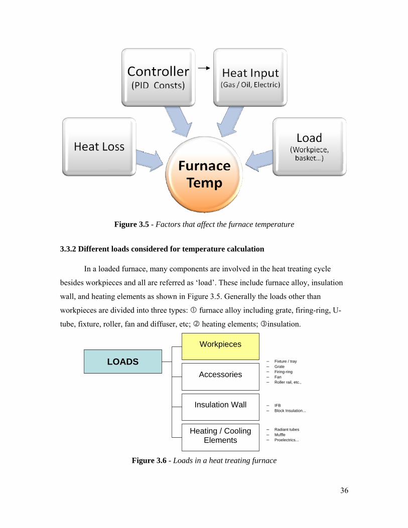
36
Figure 3.5 - Factors that affect the furnace temperature
3.3.2 Different loads considered for temperature calculation In a loaded furnace, many components are involved in the heat treating cycle
besides workpieces and all are referred as ‘load’. These include furnace alloy, insulation
wall, and heating elements as shown in Figure 3.5. Generally the loads other than
workpieces are divided into three types: furnace alloy including grate, firing-ring, U-
tube, fixture, roller, fan and diffuser, etc; heating elements; insulation.
Figure 3.6 - Loads in a heat treating furnace
LOADS
Workpieces
Accessories
Insulation Wall
Heating / Cooling Elements
– Fixture / tray – Grate – Firing-ring – Fan – Roller rail, etc.,
– IFB – Block Insulation...
– Radiant tubes – Muffle – Proelectrics...

37
Effective heat capacity calculation of furnace components
HC_fce = HC_alloy + HC_heater + HC_insulation (3.23)
where, HC_alloy is the furnace alloy heat capacity,
HC_heater is heater heat capacity,
HC_insu is furnace insulation heat capacity
3.3.3 Factors that affect the part temperature calculation
There are four main factors affecting part temperature in heat treatment, they are
part properties, part loading, part materials, and furnace condition and control, as shown
in Figure 3.7. The part temperature history in the heat treating furnace is a 3-D
conduction heat transfer process with hybrid convection/radiation boundary conditions. It
depends on the furnace temperature, working conditions, and part properties. Part load
patterns and the thermal schedule design are the main tasks in the heat treatment process
planning to guarantee the heat treatment quality. In order to simplify the temperature
calculation, three basic assumptions are made here first:
• Lumped-mass problem, i.e., temperature in part is uniform;
• Air temperature in the furnace space is uniform; and
• Convection heat transfer on the part surface is uniform.
Figure 3.7 - The factors affecting the workpiece temperature
Furnace condition and control: • Conductivity (k) • Convection (h, T_fce) • Radiation (F, T_fce)
Part properties: • Shape and sizes • Surface area and volume (A,V)
Part loading: • Weight (M_ld) • Loading patterns
Part materials: • Physical (ρ) • Thermal (cp, ε)
WorkpieceTemperature

38
In a heat treating process, parts are subjected to both convection and radiation
heat transfer. Apply the energy balance equation to the part, then,
Estorage = Econvection + Eradiation (3.27)
where, Estorage is the heat storage in the workpiece; Econvection and Eradiation are the
heat obtained from convection and radiation heat transfer, respectively.
Let the volume and surface area of the part are V and A. The energy terms in Eq. 3.27
can be calculated using following equation:
(1) Convection at ambient temperature Tfce:
( )TTAhE fceconvection −⋅⋅= (3.28)
where h is the convection heat transfer coefficient, T is the temperature of workpiece,
Tfce is furnace temperature.
(2) Radiation at heat source temperature Theater:
( )44 TTAFE fceradiation −⋅⋅⋅⋅= σε (3.29)
where ε is emissivity, σ is Stefan Boltzmann constant, F is view factor between furnace
wall and workpiece, T is the temperature of workpiece.
(3) Heat storage interior workpiece:
τρ
ddTVcE pstorage ⋅⋅=
(3.30)
where ρ is the density of workpiece, cp is the specific heat, and τ is the time.
Combine Eqs. 3.28, 3.29 and 3.30 into Eq. 3.31, then
( ) ( )44 TTAFTTAh
ddTVc fcefce −⋅⋅⋅⋅+−⋅⋅=⋅⋅⋅ σετ
ρ (3.31)
Since the part is taken as the lumped-mass body, we can imagine an equivalent
workpiece or “visual workpiece” to represent the real workpiece, as shown in Fig. 3.13.
In this way the calculation can be further simplified.

39
Figure 3.8 – The equivalent workpiece
Let V = A· t_equ, where t_equ is the equivalent thickness of the part. Apply finite
difference method to the left-side of Eq. 3.31, then
( )τδ
τδτΟ+
−=
∂∂ + kk TTT 1
(3.32)
where k is the time step. By combining Eqs. 3.31 and 3.32, at time step k, the equation
becomes,
( ) ( ) ( )( )[ ]44
_
1 kkfce
kkfce
equ
kk TTFTThtc
TT −⋅⋅⋅+−⋅⋅⋅
+=+ σερ
τδ
(3.33)
Eq. 3.33 can be used to calculate the part temperature with uniform temperature
distributions at any time in a heat treating cycle.
Above equations can be used to calculate the part temperature at arbitrary position
in the furnace. Because there are different work environment at different positions in
furnace space, the temperatures are different for different parts too. In practice, the
temperature histories of all the parts have to be considered so as to get the good products.
The effect of workpiece quantity and equivalent thickness
If lots of parts are treated in a heat treat cycle, we have to assure that all the parts
are well heated during the process. It is not necessary to calculate the temperature-time
profile for every part in furnace. Instead, the temperature-time profiles of some typical
parts are considered in the furnace (such as the parts close to furnace wall and in the
(a) Real workpiece (b) equivalent workpiece
t equ
x
y
z
40
middle of furnace). The part load effect on the part temperature is mainly contributed
from the radiation heat transfer and will be discussed in a later section.
The reason to calculate equivalent thickness is that sometime we need not only
the surface temperature on the workpiece, but also the core temperature. This is a simple
method used to calculate the interior temperature of a part. There are several methods that
can be used to calculate the equivalent thickness of a workpiece. The calculation methods
will depend on the load conditions and calculation methods:
• The minimum dimension of heaviest cross section in workpiece
• The value of workpiece volume divided by surface area: t_eff = V/A
• The value of 3 times of volume divided by surface area: t_eff = (3·V)/A
• The value of volume divided by exposition area to heater: t_eff = V/A_exposition
In our development of CHT, the first method is used as default value which can be
changed through a user interface.
The effect of convection heat transfer
In practice, the convection heat transfer around part surface is not uniform. This
can be described using convection film coefficient h. Following is one of the calculation
methods for the coefficient h:
h = (k ⋅ Nu) / L* (3.34)
where Nu is Nusselt number, a dimensionless heat transfer coefficient, and can be
calculated using an experimental equation[11]:
Nu =c⋅ Rem (3.35)
where Re is Reynolds number, a dimensionless group charactering a viscous flow; the
characteristic dimensions c and m are calculated from experimental values. Note that this
equation is only used to gases medium.
Re = (V ⋅ L*) / ν = (ρ ⋅V ⋅ L*) / μ (3.36)
where L* is a characteristic length of the part; k is the thermal conductivity; V is air
velocity; ν is the kinematic viscosity; ρ is density; and μ is dynamic viscosity.

41
The effect of radiation heat transfer
Because the parts are located in the different positions in the furnace, the heat
they receive from the radiation transfer are different. This effect can be represented by
the view factors. The value of view factor is affected mainly by the distance between
furnace wall and the part, as well as the shadowing among workpieces. A CAD-based
method of calculating the view factors is developed, the view factors can be specified
based on the CAD-based calculation method.

42
3.4 Furnace temperature control model The furnaces are controlled by temperature controllers. The temperature
controllers get their inputs from a thermocouple located inside the furnace and send
necessary control action to the burner to maintain the process setpoint.
Figure 3.9 - Schematic of the Temperature controller in a radiant tube type furnace.
3.4.1 Commonly used schemes in heat treatment furnaces
The control action for the temperature controller can be either on/off or proportional.
Process tolerances and the final device being controlled normally determine the type of
control action.
On/off control is simple to understand. For example in a heat treat furnace during
the heating process, if the measured process temperature is below the control setpoint,
burners are continuously fired by the controller. If the measured value exceeds the control
setpoint, the controller shuts the burners. Switching the heat on and off takes place at
setpoint. This type of control causes the process value to oscillate around the control
setpoint.

43
Figure 3.10 - On/Off & Proportional type controllers commonly used in furnaces.
Proportional control (PID) is a more sophisticated control approach which results in
tighter control around a setpoint and less process oscillation.
Proportional control consists of 3 basic control functions:
1. Proportional band
2. Reset, or Integral
3. Rate, or Derivative
Proportional band is the process range over which proportioning control action takes
place. In a heating situation, if the process temperature is below the proportional band,

44
burners are continuously fired by the controller. If the process value is above the
proportional band, the burners are shut. Within the proportional area, as the process
temperature increases the amount of heat being called for decreases proportionately. (as
shown in Fig 3.15 where T1, T2, T3… are the proportionally decreasing time values)
To determine the proper proportional band setting, the time required to approach setpoint
must be balanced with the processes' ability to withstand overshoot. If proportional band
is too narrow, the heat input will not be cut back soon enough and the process will
overshoot. A wide proportional band begins cutting back the heat input sooner. A narrow
proportional band (means heat is on longer) will approach setpoint quicker than a wide
proportional band.
Reset (Integral) shifts the proportional band in relation to the desired setpoint. Reset
action is used to compensate for sustained process offset from the control setpoint.
Rate (Derivative) is used to compensate for initial overshoot and sudden process
disturbances. Rate will temporarily compress the proportional band around setpoint to
bring the process under control.
3.4.2 Controller tuning
It is necessary to tune a controller to a particular process. This will enable the
controller to maintain tight control of the process. This will remain so even if process
variables (ambient temperature, load size, hearth/gasket condition, etc.) change over time.
Properly tuning a controller to a process is an absolute necessity to ensure tight
control. Manually tuning a controller is a time consuming and tedious exercise. There are
several features available in today's controllers which facilitate tuning. Autotune
capability now allows a controller to tune itself to a process. Autotune will introduce a
minor process disturbance and this enables the controller to determine how the process
should react to the change and the amount of time required to recover. Based on these
parameters the controller determines the necessary constants.
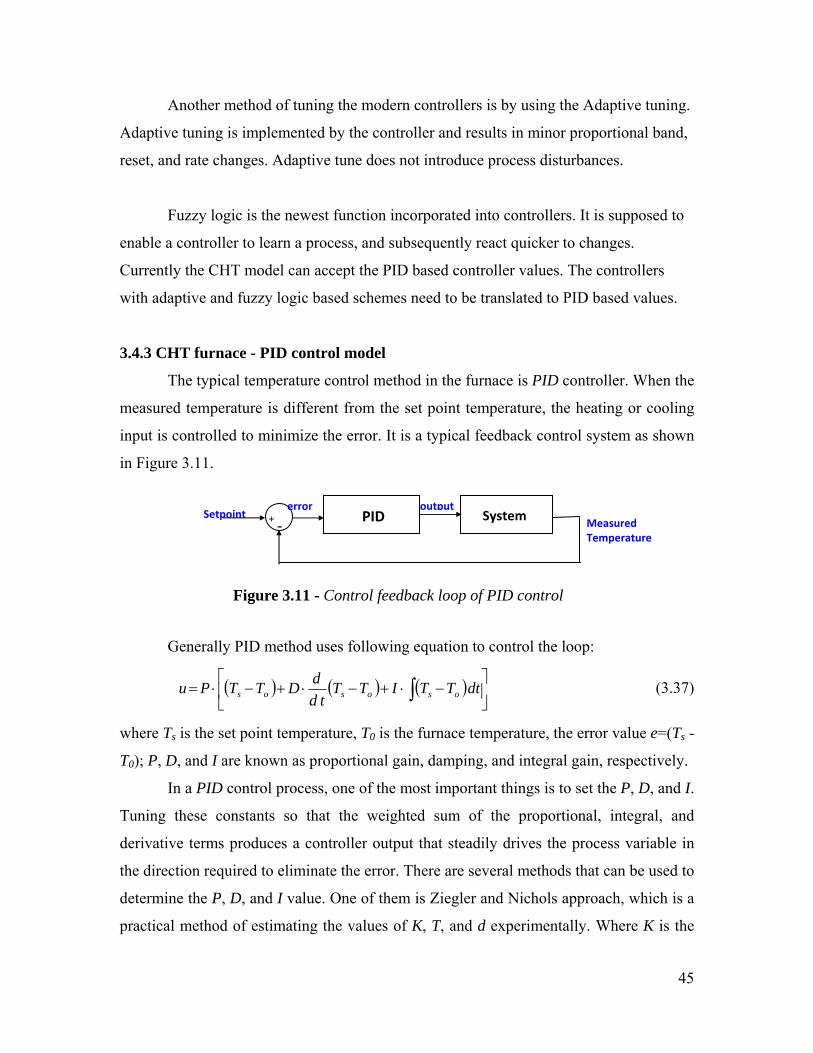
45
Another method of tuning the modern controllers is by using the Adaptive tuning.
Adaptive tuning is implemented by the controller and results in minor proportional band,
reset, and rate changes. Adaptive tune does not introduce process disturbances.
Fuzzy logic is the newest function incorporated into controllers. It is supposed to
enable a controller to learn a process, and subsequently react quicker to changes.
Currently the CHT model can accept the PID based controller values. The controllers
with adaptive and fuzzy logic based schemes need to be translated to PID based values.
3.4.3 CHT furnace - PID control model
The typical temperature control method in the furnace is PID controller. When the
measured temperature is different from the set point temperature, the heating or cooling
input is controlled to minimize the error. It is a typical feedback control system as shown
in Figure 3.11.
Generally PID method uses following equation to control the loop:
( ) ( ) ( ) ⎥⎦
⎤⎢⎣
⎡−⋅+−⋅+−⋅= ∫ dtTTITT
tddDTTPu ososos (3.37)
where Ts is the set point temperature, T0 is the furnace temperature, the error value e=(Ts -
T0); P, D, and I are known as proportional gain, damping, and integral gain, respectively.
In a PID control process, one of the most important things is to set the P, D, and I.
Tuning these constants so that the weighted sum of the proportional, integral, and
derivative terms produces a controller output that steadily drives the process variable in
the direction required to eliminate the error. There are several methods that can be used to
determine the P, D, and I value. One of them is Ziegler and Nichols approach, which is a
practical method of estimating the values of K, T, and d experimentally. Where K is the
PID System+ -
Figure 3.11 - Control feedback loop of PID control
Setpoint error output
Measured Temperature

46
process gain used to represent the magnitude of the controller's effect on the process
variable, T is the process time constant used to represent the severity of the process lag,
and d is the deadtime used to represent another kind of delay present in many processes.
With the controller in manual mode (no feedback), a step change is included in the
controller output and the process reaction is analyzed. The process gain P can be
approximated by dividing the net change of the process variable by the size of the step
change generated by the controller. The dead time is estimated from the interval between
the controller step change and the beginning of a line drawn tangent to the reaction curve
at its steepest point. They are also used the inverse slope of that line to estimate the time
constant T.
dKTP⋅⋅
=2.1
2
6.0dKTI
⋅⋅
=
KTD ⋅
=6.0
Sometimes, when the sensor measuring the furnace temperature is susceptible to
other electrical interference, derivative action can cause the heater power to fluctuate
wildly. In this case D = 0, and a PI controller is often used instead of PID controller. The
typical application of PD control in furnace is to control heat/cool gases input. The
adjustment coefficient of heat input, Htg, is calculated using following equation:
( ) ( )∫ −⋅⋅
+−⋅=τ
0 ____ fcespfcesp TTSpan
IGPGTTSpanPGHtg (3.39)
where the proportional gain PG=10 and the integral gain IG=0.05.
(3.38)

47
3.5 Summary
The CHT furnace model is a comprehensive model with a capability to model
several different types of furnaces and control schemes. Currently there are several
proprietary models used internally by the industry that is not publicly available. The CHT
model is the most comprehensive model currently available to the industry and is in use
at several CHT member companies since 2002. The model used in the CHT software
system and has been validated with several case studies.

48
CHAPTER - 4 Furnace model analysis The experiments conducted using the CHT software at various customer locations
are listed in Appendix-A and grouped by Furnace type and the results are analyzed. The
CHT-b/f & CHT-c/f calculated results are compared to the measured thermocouple
results. The comparison between the results are performed by focusing on the following
areas / issues,
• Heat up rate accuracy
• Time taken to reach furnace setpoint (comparision)
• Accuracy of soak time and temperature
• Abnormal peaks – gradients, flame screens,…
Each area with high error percentages was analyzed to determine the cause of the
problem. Some minor problems were attributed to software bugs which were fixed later.
The major problems were studied in detail and expert opinion from the shop floor was
requested to further understand the problem. A detailed list of problems in the current
model due to furnace issues like gradients, furnace aging, and the model constraints are
documented. The results presented in this chapter as based on the observations and
conclusions based on the experimental results documented on Appendix – A.

49
Table 4.1. List of case studies in different furnaces and locations
Furnace Type Company Location Number of experiments
Continuous Furnaces
American Heat Treating Monroe, CT 4 Bodycote Waterbury, CT 6 Worcester, MA 1 Caterpillar Peoria, IL 13
(24)
Vacuum Furnace
Bodycote Worcester, MA 4 Bodycote South Windsor,
CT2
Bodycote Wisconsin 2 Sousa Corporation CT 1 American Heat Treating Monroe, CT 5
(14) Batch Furnace Bodycote Worcester, MA 12
American Heat Treating Monroe, CT 1 Surface Combustion Maumee, OH 1 Queen city steel Cincinnati, OH 1
(15) Total 53
4.1 Furnace model study
To breakdown the analysis task, the model was studied from three practical perspectives,
1. Structural model
2. Control schemes model
3. Process related parameters

50
4.1.1 Structural model
The furnace was studied from a structure stand point and several factors were
classified and important to the accuracy of the model. The several problems and their
effects are listed below.
Universal furnace
The current model is universal for all furnaces. Due to this issue its unable to calculate
the heat losses that are more specific to certain kinds of furnace. The effect of having a
universal furnace is in the improvement in the accuracy certain heat loses and heat heat
storage in the furnace (Q_fce) if we have more specific furnace categories. (eg: Vacuum,
Box, Pit, etc.,)
Burner locations
Thermal gradient in the furnace due to location of the burners and their BTU’s. There is a
thermal gradient inside the furnace and the BTU is not distributed uniformly inside.
Current model assumes uniform furnace temp. And Accuracy issues especially in
Continuous furnaces.
Atmosphere flow
The effect of atmosphere flow and calculating a constant to adjust the heating parameters
due to the heat losses. These result in accuracy issues. Case studies done for validation in
the atmosphere furnaces show the inconsistency especially during heat up.
Incomplete accessory data
Make a generic list of accessories for each kind of furnace. Improves the model accuracy
by considering all the furnace elements.
4.1.2 Control model
Similar to the structural model all the elements that contribute to the furnace
control were studied separately and their effects are listed below.

51
Furnace controller
In the current model there is no option to specify the exact control schemes used in the
furnace. This results in aprroximation of the control scheme that is deployed in the shop
floor.
Multiple controllers
There is no option to specify multiple controller parameters for different zones. Also the
controllers are tuned differently for different zones based on the process parameters
especially in the continuous furnaces. These result in inaccurate thermal profile
calculation.
Control thermocouple
There is often a thermal gradient inside a furnace and one of the reasons is due to the
location of the control thermocouple. Currently the model assumes a uniform temperature
distribution. The control thermocouple location information helps to calculte the gradient
present inside the furnace.
4.1.3 Process parameters
Several processes require the furnace to be controlled differently. The main differences
are in the atmosphere control and the temperature control. The experiments were
conducted for the current list of processes,
1. Annealing
2. Tempering
3. Carburizing
4. Brazing

52
4.2 Problem identification in the current CHT furnace model A detailed study of the experimental analysis based on Furnace classification,
Control schemes and Process related parameters revealed the following limitations or
issues in the current CHT model. Several of these also have an effect on the model
accuracy.
1. Universal furnace model
The current model is based on an universal model for all furnaces. Hence it
cannot accurately calculate the heat losses that are more specific to certain kinds
of furnaces. (eg: Vacuum, Box, Pit, etc.,)
2. Burner locations
Current model assumes uniform furnace temperature, often there is a thermal
gradient in the furnace due to location of the burners and their capacities.
3. Atmosphere flow
Case studies done for validation in the atmosphere furnaces show the
inconsistency especially during heat up. The effect of atmosphere flow and the
heat losses and heat transfer affects the accuracy of the model.
4. Furnace accessories
Furnace accessories like baskets, fixtures, etc, also consume heat inside furnace
along with the load. The current model uses a generic fixture approximation.
5. Door operations
The current furnace model does not take into effect the heat loss arising due to the
door operations during charging and discharging the parts from the furnace. From
the experimental analysis this was not an issue in Batch furnaces but it had an
impact on the continuous furnaces.

53
6. Furnace controller
Inability to translate the control schemes used in the furnace to the PID based
control in the furnace model.
7. Multiple furnace controllers
The furnaces often use multiple controllers for different zones. The controllers are
tuned differently for different zones based on the process parameters, especially in
the continuous furnaces. Currently CHT model uses a universal controller.
8. Control thermocouple location
It was found a thermal gradient inside the furnace may be present due to the
location of the control thermocouple.
9. Process data
Several processes require operating the furnaces differently. (For example, in the
carburizing furnace, the enriching gas is added to the furnace after the load
reaches the temperature. The ability to specify in the CHT model the amount of
gas added in the cycle improves the calculation of heat loss, which is currently not
possible)
10. Proprietary furnace control schemes
The furnace and controller manufacturers use several proprietary furnace control
techniques. Its difficult to model these control schemes. (for example – its
difficult to determine the PID constants (for CHT model) from a controller tuned
with an adaptive tuning algorithm)
11. Furnace deterioration (wear/tear)
The furnace refractory and burners deteriorate over time, increasing heat losses
and reducing heat available respectively.

54
12. Faulty or incorrectly tuned burners
The burners need to be tuned properly for complete combustion. An incorrectly
tuned burner or a faulty burner does not produce the specified heat.
4.3 Summary & conclusions After analyzing all the list of limitations and problems in the current CHT furnace
model the following were determined to have significant effect on the furnace model
accuracy.
1. Heat loss due to door operations
2. Thermal gradients inside the furnace
3. Furnace deterioration over time
The heat loss in the furnace due to door operation is a problem more significant in
continuous furnaces than batch furnaces. With several experimental data and modeling
we can develop new model to incorporate in the CHT model to account for this loss. The
thermal gradients present inside the furnace is a complex phenomenon, it is caused due to
several factors like burner and control thermocouple location, the furnace construction,
etc., and it is also unique to every furnace, so more detailed study is required to
understand and model this phenomenon. Furnace wear phenomenon can be modeled by
conducting calibration experiments with virtual load and the parameters reverse
calculated. These are the development proposed for the improvement of the CHT furnace
model.

55
CHAPTER - 5
Improved furnace model
5.1 Introduction
The Furnace Model Analysis study gave an insight on the current CHT Furnace model’s
shortcomings and opportunities to improve the overall accuracy. From one of the experimental
results on a Continuous Pusher Furnace (as seen in Fig. 5-1a) we can see a significant thermal
gradient present inside the furnace in the holding chamber and also there was a wave due to the
heat loss from the door openings and the controller action. This problem is specific to this type of
furnace and more due to the design and arrangement of the burners.
Time (min)
Tem
pera
ture
(°C
)
20 40 60 80840
850
860
870
880
Northwest 1Northwest 26North 1North 26Northeast 1Northeast 26
Figure 5.1a - The thermal gradients inside a Continuous Pusher Furnace,
experimental data from continuous datapak with 6 thermocouples.

56
Based on the furnace model analysis presented in the earlier chapter and from discussion
with customers and experts, the key focus was narrowed down to 3 specific problems,
(i) Heat loss due to furnace charge / discharge door operations (specific to continuous furnaces)
(ii) Thermal gradients present inside the furnace
(iii) Furnace deterioration and related inaccuracies in the model.
The new model is represented as follows by addition of 3 new terms to the original equation,
(5.1)
where, kfceT = Furnace temperature (at time step, k)
kdoorfceT _Δ = Furnace temperature variation due to door operations
),,(_ zyxT kgradientfceΔ = Temperature gradient inside furnace in 3D space
kvirtualfceT _Δ = Furnace calibration using virtual load
Detailed explanation of the 3 terms, how they are calculated and used in the model are
described in the following chapters. Experimental case studies are also conducted to verify the
results.
kvirtualfce
kgradientfce
kdoorfce
kfce
kfce TzyxTTTT ___
1 ),,( Δ+Δ+Δ+=+

57
5.2 The door open model ( kdoorfceT _Δ )
The CHT model does not calculate the heat loss and the heat exchange between zones
that occur as a result of the door operation. Currently the furnace temperature is not calculated in
the continuous furnace model based on the PID control. The calculated furnace temperature does
not reflect the variation observed in the experiments. This chapter discusses addition of a heat
term to compensate for the heat loss arising out of door operations.
5.2.1 Introduction
A series of experiments were conducted at a beta test facility to evaluate the accuracy of
the continuous furnace model under different conditions. The experiments were conducted on a
brand new furnace undergoing production trails. This helped us eliminate some of the guess
work out of calculation especially the heat loss factor due to the physical wear and tear of the
furnace. After conducting the experiments a significant variation between furnace set-point
temperature and the measured workpiece temperature (around 25°C) was noticed. There also
existed a uniform pattern to the thermal profiles in all the experiments. This pattern matched with
that of the door open sequence. This thermal pattern is shown in the Fig.5-1b.
Time (min)
Tem
pera
ture
(°C
)
110 115 120 125 130
840
850
860
870
880
North 1North 26NW 1NW 26NE 1NE 26CHT Calculated
Figure 5.1b - The thermal profile of the CHT calculated and measured workpiece
temperature at 6 different locations in a Continuous Furnace.

58
The current furnace model (CHT model) was developed based on the batch furnace
model and the main assumptions in the model are,
(i) The furnace temperature does not change with varying load conditions. It always remains
same. (So the heat balance is not calculated and PID control is not considered either)
(ii) The workpiece movement is considered linear. (either step movement or continuous)
(iii) The workpiece is fixed and the furnace is moving. So the thermal schedule is a function
of the movement speed. The furnace temperature is the same as thermal schedule.
(iv) The heat transfer at the calculated domain boundary to other loads is zero.
Zone 1 Zone 2 Zone n
vstep
Calculationdomain
row
column
layer
Figure 5.2 - Pusher type Continuous Furnace Model
With the workpiece as a reference, the furnace temperature involved in the calculation
changes with the workpiece row number and time, as shown in Fig.5-2 the temperature is
calculated for different zones. The furnace temperature distribution is a function of furnace zone
and corresponding transition zone. It is depicted as follows:

59
⎪⎪⎩
⎪⎪⎨
⎧
−<<+
+≤≤−−−+
−+
=
∑∑
∑∑∑
=
−
=
+===+
+
j
j
iij
j
iizonej
j
j
iij
j
iij
j
ii
jj
zonejjzonezonej
fce
LLdLLT
LLdLLLLdLL
TTT
dT
0
1
0_
10001
_)1(__
_
))(()(
(5.2)
where,
i and j are the zone numbers,
d is the distance from the beginning of the furnace, in the range of 0 to the whole length of the
furnace; L is the length of furnace zone.
Since the temperature variations observed during the experiments were significant from a
heat treatment processes stand point, it was decided to integrate new terms to the current
Continuous Furnace model to improve the furnace temperature accuracy to reflect the real world
conditions.
There are two modes of heat loss arising due to the door operation. A radiation heat loss
and heat loss due to the exchange of the furnace gas between zones and to the atmosphere in the
final zone. There are several doors in the furnace between zones.

60
Figure 5.3 - Door open/ Push sequence in a Continuous Furnace Model
As illustrated in Fig. 5-3 the door open sequence can be simulated starting from a fully
loaded furnace. The door 5 is opened through a slot door for quenching, during this operation
there is a radiation heat loss and also heat loss due to the loss of furnace atmosphere. Once the
door 5 is closed the door 4 opens and parts are pushed in the final zone. During this operation
there is a heat exchange through radiation depending upon the zone temperatures and normally
there is not a significant amount of atmosphere exchange. (Assumed based data on the pressure
variation during the door operation is presented later). The same sequence of operations follow
during the operation of doors 3 and 2. When the door 1 opens a new cold part is loaded in the
furnace. We do not model the first few zones, as there is a significant cold mass entering the
furnace. There is no temperature swings in the first few zones and the burners are firing at the
maximum rate to achieve the set-point temperature.

61
Figure 5.4 - Empirical data used by a furnace manufacturer based on experiments
and experience to predict the loss of atmosphere during the door
operation in a continuous furnace
The atmosphere exchange and heat loss in the final zone is complex as shown in Fig.5-4.
When the slot door opens, due to the pressure differential the furnace hot atmosphere escapes the
furnace and at the same time there is cold air entering the furnace due to the vacuum created
inside the furnace. This happens due to a drop in the furnace atmosphere volume because of the
heat loss. It’s difficult to calculate the exact volume of atmosphere lost and air added. Based on
experimental data presented from a furnace manufacturer the velocity of hot air leaving the
furnace is around 500-600 ft/min and usually this takes place in the top 1/3 space of the slot
door. And the cold air velocity entering the furnace is around 100-200 ft/min.
5.2.2 Experiments on pressure differences between zones & during door operations
Further experiments were conducted to understand the gas exchange between the
different zones in the furnace and to the atmosphere during the door operations. A series of
experiments were conducted to study the pressure in the different zones in the furnace and the
changes in pressure during the door operation.

62
Time (minutes)
Pre
ssur
e(H
2O")
0 5 10 15 200.05
0.1
0.15
0.2
DUNK QUENCHHOLDING CHAMBER
Figure 5.5 - The pressure in two different final zones in a Continuous Pusher Furnace
Figure 5-5 shows the plot of pressure in Holding Chamber and Dunk Quench Chamber in
inches of water (27.7 inches of Water = 1 PSI at 62° F). The pressure inside the furnace is
slightly above the atmospheric pressure. Also the pressure in the holding chamber is maintained
above the dunk quench chamber to prevent the gas from entering the holding chamber. This is
done to prevent decarburization in the holding chamber.

63
Time (minutes)
Pre
ssur
e(H
2O")
0 5 10 15 20 25-0.5
0
0.5
Hol
ding
/Dun
kIn
nerd
oor
Diff
use/
Hol
ding
Slot
Doo
r
Allig
ator
Time (minutes)
Pre
ssur
e(H
2O")
0 5 10 15 20-0.5
0
0.5
1
Alli
gato
r
Hol
ding
/Dun
kIn
nerD
oor
Hol
ding
/Dun
kIn
nerD
oor
Diff
use
/Hol
ding
Alli
gato
r
Slo
tDoo
r
Slo
tDoo
r
Figure 5.6 - The pressure variations as a function of different door operations events.
Holding Chamber (left) & Quench Chamber (right)
As observed in Fig. 5-6 the pressure variations in the different zones are plotted as a
function of the different door operation events. One of the observations is that the door openings
in a zone had an effect on the pressure on several different zones. It had a clear influence on the
pressures in the adjacent zones and this implies that the intermediate zone doors are not pressure
tight and hence there is exchange of gases that takes place during the door openings.
The negative pressure formed after the door operation is created due to the reduction in
volume of gas. When the door opens a significant amount of air enters the furnace and creates
combustion of the endothermic gas present in the zone. When the door closes, pressure spikes
due to the expansion of the gas due to higher temperature resulting from the combustion. And the
combustion stops once all the oxygen is consumed from the air and this result in a significant
reduction in the temperature and volume causing the pressure to go in the negative.
Based on the experimental data on temperature and pressure a new term was added to the
current Continuous furnace model to account for the heat loss.

64
5.2.3 Modified model to include door open term
(5.3)
where, q_dopn is the heat loss caused by radiation and mass loss during doors operation. , q_dopn is
also a function of time calculated from the door open schedule.
Figure 5.7 - The door open schedule based on the furnace layout represented in the time domain
An assumption was made for creating the door open schedule. The door is either open or
closed so the intermediate positions are not considered in the schedule as shown in Fig.5-7.
The q_dopn is calculated based on the following equations,
(5.4)
dopnfanclldlosshtstorage qqqqqqq _______ −+−−−=
⎩⎨⎧ +
=doorlast not the while,
doorlast the while,
__
______
raddopn
exchangeairdopnraddopndopn q
qqq

65
(5.5)
(5.6)
As shown in equation (5.4) another assumption was made based on the experiments that
there is not significant loss of heat in the intermediate zones due to the air exchange.
exchangeairdopnq ___ is calculated only for the last zone.
(5.7)
where,
d is the equivalent diameter of the door,
λ is the coefficient of heat conductivity,
l is the thickness of the door, R is the gas constant,
p_fce is the pressure in the door,
p_door_outside the pressure outside the door, and
kd is the empirical coefficient of heat convection (for the current furnace its 3.5 m/s based on the
pressure experiments.
⎩⎨⎧
=closedoor while,0
opendoor while,)( ,_
_mdoor
open
AA τ
( )4__
4____ )( outsidedoorfceopenraddopn TTAq −⋅⋅⋅⋅= τσεη
( )
( )outsidedoorfced
outsidedoorfceoutsidedoorfcefce
exchangeairdopn
TTkc
TTpplRT
dcq
___
___2
__2_
_
52
___ )(16
−⋅⋅=
−⋅−⋅⋅=λπ

66
Figure 5.8 - The screen shot of the furnace thermal profile computed by
CHT-c/f software using the improved furnace model
As observed in Fig. 5-8 the new thermal profile computed using the improved furnace
model reflects the furnace temperature drops due to the door operation in the first and the final
zones. This plot also shows the effect on the part temperature due to the variation in the furnace
temperature. Another experiment was conducted to verify the improved furnace model.

67
Time (minutes)
Tem
pera
ture
(C)
40 45 50 55 60
850
860
870
880
890
900
Measured (datapak NW1)Calculated (CHT-c/f Furnace)
Figure 5.9 - The comparison of the furnace thermal profile computed using
improved furnace model and measurement results.
As seen from the above Fig. 5-9 as well as from Fig. 5-8 the computed results now take
into account the heat loss due to the furnace door operations. Fig. 5-9 also illustrates that the
calculated furnace thermal profile is in good agreement with the measured results. This helps
in accurate calculation of the part temperature profile especially in the last zones where the
temperature of the part is critical in carburizing operations.

68
5.2.4 Conclusions
The new improved model was verified with experiments to take into consideration the
heat loss involved with the door operations. The same modeling method can be used to
determine the heat loss involved with other type of continuous furnaces, but in this study the
model was verified only with the Pusher type continuous furnaces. Some of the problems
with this new door model are: to accurately determine the heat loss due to door opening, and
to differentiate the peaks arising due to the PID controller. The key to accurately determine
the door opening peaks is to understand and filter the false peaks arising out of the controller
activity.

69
5.3 The furnace gradient model ( ),,(_ zyxT kgradientfceΔ )
5.3.1 Introduction
The furnace temperature gradient is a phenomenon that exists inside a furnace due to non
uniform heating. This non uniformity in temperature directly affects the part temperature profile.
And it has direct impact on the heat treating processes. For example a carburizing process
operating at a carbon potential of 1% and running at 927 °C yields a 1.35mm case depth. If the
carburizing temperature is reduced to 850 °C the carburized case depth achieved is only 0.8mm
(for the same material and same carburizing duration a 40% reduction)
Figure 5.10 - The thermal gradients inside a batch type heat treating furnace[6]
The Fig 5-10 shows a thermal image captured inside a batch type heat treating furnace.
There is a 22 °C variation (Max. 1692 & Min 1621 Fig. 5-10-right) with no load in the furnace.

70
5.3.2 Study of thermal gradients in continuous furnace (at 2 locations in 4 zones)
Figure 5.11 - Furnace temperature gradients and gradient variations in a fully loaded furnace
over a period of 40 minutes in a Continuous Pusher type Carburizing Furnace
with a push cycle time of 16 minutes.
Another experiment was performed to study the effect of load and the thermal gradient
and variation in the gradient over a period of time in a continuous furnace. A carburizing type
Setpoint
Temp
°C

71
pusher furnace was selected for the experiment and two thermocouple locations were selected.
The first thermocouple was inserted close to the control thermocouple location, which is located
near the top wall of the furnace above the burners and the second thermocouple was inserted
through the shim port on the side wall of the furnace and was inserted around 6” from the inside
wall of furnace. The temperature data were recorded simultaneously using two different data
recorders. To check the repeatability of the experiments since two different experimental setups
(different type of data recorders) were used, the experiments were repeated in Boost Zone 2 (B2)
by swapping the control and shim setup after the first experiment was completed. As shown in
Fig. 5-13 they had a good repeatability and the error was within 0.5°C, this gave us confidence to
go ahead with the rest of the experiments in the other zones with two different experimental
setups.
As observed in Fig. 5-11 furnace zones boost 1 and boost 4 (B1 & B4) had the highest
average temperature gradient (ΔTAVG) 14.6°C and 18.4°C respectively. And coincidentally the
temperature variation was also the highest at the shim location in the zones B1 and B4 which
was recorded over a period of 40 minutes. At the time of the experiments the furnace had a push
time of 16 minutes, so 40 minutes gave an opportunity for the thermocouples to gather data over
two push cycles. There were several observations made from the collected data. The TAVG was
always less than the median value (the data was collected at 10 second intervals and averaged).
Also at the locations B1 and B4 where the temperature gradients were highest the TAVG was
closer to the min value. So from the experiments it can be concluded that the load has an effect
on the furnace thermal gradient (ΔTAVG ).
5.3.3 Study of thermal gradients in pusher furnace
As discussed in the earlier door open model, when we conducted experiments to evaluate
the accuracy of the continuous furnace model we came across thermal gradient problem that
prevails in several industrial heat treat furnaces. In this particular furnace in which we were
conducting experiments, the thermal gradients were significant (around 30°C) especially in the
last zone due to the complex design of the furnace and lengthy radiant tube burners. Fig. 5-12b

72
illustrates the experimental temperature data collected using a datapak device with 6
thermocouples placed at different locations. Fig 5-12a shows the experimental setup and the
location of the thermocouples.
Figure 5.12a - Experimental setup showing the datapak and
thermocouple locations inside the Pusher Furnace.
Time (min)
Tem
pera
ture
(°C
)
20 40 60 80840
850
860
870
880
Northwest 1Northwest 26North 1North 26Northeast 1Northeast 26
Figure 5.12b - The thermal gradients inside a Continuous Pusher Furnace,
experimental data from continuous datapak with 6 thermocouples.

73
The thermocouples were placed in two groups, first set of 3 thermocouples were placed
1” from the top of the fixture grid and the second set of 3 thermocouples were placed 26” from
the fixture grid. The thermocouple locations were marked North, Northeast and Northwest.
North being the furnace push direction as shown in Fig. 5-12a. From the experiments it was clear
the thermocouples that were located 1” from the fixture grid had a lower temperature compared
with the rest of the thermocouples and this was significant in the last zone of the furnace. In
certain locations where the furnace temperature drop was more than 30°C, it had a huge impact
on the accuracy of the calculated furnace and part temperatures in the CHT furnace model.
5.3.4 Study of thermal gradients in rotary type continuous furnace (at 2 planes & 12
locations in 3 zones)
Since most of the experiments were conducted in continuous pusher type furnace several
more experiments were conducted in different types of continuous furnaces to study the
prevalence and the extent of the thermal gradients inside the furnaces.
Figure 5.13 - Temperature gradient between the set point temperature
and the work area (center of furnace) at 3 different zones and locations
in a Rotary type Continuous Furnace
SETPOINT ‐ M
EASU
RED

74
Figure 5-13 shows the thermal gradients present inside a rotary type continuous furnace.
The different bars in the chart indicate 3 different zones (B – Boost zone, D – Diffuse zone and
E – Equalize zone) and 4 different locations (1, 2, 3 and 4) in each zone. At the time of the
experiments the Boost zone was at 927 °C, Diffuse zone was at 880°C and the Equalize zone
was at 850 °C. All the four locations where the temperatures were measured were in the same
place (near the work pieces). As seen in the graphs the Boost zone had the highest temperature
difference between the setpoint thermocouple and the measured results. Again a 16 °C
inaccuracy in the CHT furnace model due to the gradient that is present in the furnace is
significant.
5.3.5 Gradient patterns
It is important to understand why thermal gradients exist inside the furnace. It is a
complex issue to study all the possible gradients that exist inside the furnace. So only the
gradients that are significant to the process and quality of the product are focused. In a
carburizing furnace 10°C variation in the temperature in the boost zone affects the carbon
potential by 3% and in the diffuse zone a 10 °C variation in the temperature affects the carbon
potential by 10% C so any temperature variation in the 10 °C magnitude has consequences for
the product quality.
Several experiments were conducted in different furnaces to determine the thermal
gradients and the gradients that were more than 10°C from the set point temperature were
analyzed. Out of the several possible causes the most predominant occurrence in the thermal
gradient was when the burners were not symmetrically placed (for example if there were not
equal number of burners on top and bottom of the furnace). It was observed in the experiments
that if a zone has a long radiant tube burner a thermal gradient was present. The different burner
schemes or layouts that are commonly used in the furnaces are shown in Fig. 5-14. As shown
there are three different schemes that are commonly used,
1. Equal number of burners on top and bottom 2. Unequal number of burners (more burners on one side) 3. Burners on only one side (only on top)

75
Figure 5.14 - Different burner patterns / schemes commonly used in the
Pusher Type Continuous Furnaces
Several experiments were conducted with furnace with all three burner configurations.
The case (iii), when there was burner present only on top side had the highest gradients observed.
Fig. 5-15 shows the thermal gradients present in a furnace inside different zones. The zones 1-4
had equal number of burners on top and bottom. And zone 5 had burners only on the top.
5.3.6 Effect of burner layout on gradient patterns
As illustrated in Fig 5-14 there is a different layout of burners used in different zones of
the continuous furnaces depending on the furnace design parameters. Usually the initial zones
have the most number of burners with maximum energy to bring the parts to temperature as soon
as possible. And different furnace manufacturers design and locate the burners differently inside
the furnace. An experiment with a continuous pusher type furnace was conducted and the time
scale was translated to distance and the effect of burner layout is analyzed. The burner layout
pattern had a direct effect on the gradient patterns. The zone 5 had burners only on the top wall
and no burners in the bottom and also due to the furnace design it had long burners.

76
Figure 5.15 - Thermal gradients measured at different locations in a
Pusher type Continuous Furnace with different zones marked.
From the graphs above in Fig 5-15 we can clearly see a gradient of almost 30°C is
present. Also Holding Chamber (5 in Fig-5-15) had a long radiant tube so this created another
variation in the temperature along the length of the radiant tube burner.
5.3.7 Different common burner layout types and gradient pattern (at furnace cross
sections)
In order to understand the burner layout effects on the thermal gradient, a series of
experiments were conducted in a relatively old continuous pusher type furnace that had all the 3
types of burner layouts in the different zones. A thermocouple was inserted at a location directly

77
underneath the burner through the hole on the top of the furnace and the temperature was
measured for 2 parts pushed in the furnace and the average temperature was recorded. And the
thermocouple was lowered into the furnace 1/3, 2/3 the total distance and all the way down from
the top wall and measurements were repeated.
Figure 5.16 – The top view of boost zone with thermocouple locations and the corresponding
shim port locations for the data gathered.
And the thermocouple was inserted into the side wall through the shim port of the furnace
wall and the temperature was recorded near the furnace wall. And another data was recorded by
inserting the thermocouple thorough the gas port located just above shim port on the side of the
furnace wall. Fig. 5-16 shows the location of ports locations.

78
temp
Furn
ace
(Dis
tanc
e%
)
900905910915920925930
0
20
40
60
80
100BOTTOM
TOP
Figure 5.17a – The measured temperature gradient pattern inside furnace
– Holding Chamber (Burner layout – I)
Temperature (C)
Furn
ace
(Dis
tanc
e%
)
900905910915920925930
0
20
40
60
80
100BOTTOM
TOP
Figure 5.17b – The measured temperature gradient pattern inside furnace (Burner layout – II)

79
Temperature (C)
Furn
ace
(Dis
tanc
e%
)
900905910915920925930
0
20
40
60
80
100BOTTOM
TOP
Figure 5.17c – The measured temperature gradient pattern inside furnace (Burner layout –III)
The Fig. 5.17 a, b & c represent the various gradient patterns that exist inside the furnace
measured at 3 cross sections across the furnace. The next task was to use this cross-sectional data
Figure 5.18 – The gradient generated across the entire furnace using the static experiments.
Distance (feet)
° C

80
to generate the gradient pattern across the entire furnace length. The interpolated data generated
from the cross sectional experimental gradients is shown in Fig. 5.18.
5.3.8 Furnace gradient model development
A new improved furnace model is developed in order to calculate the furnace temperature
accurately by accounting the thermal gradients. A new term is added to the existing model to
calculate the furnace temperature. The kgradientfceT _Δ is calculated based on the experimental data.
Also a load constant A is included in the equation to account for the load size. The constant A is
dependent on the size of the load that was used to determine kgradientfceT _Δ .
(5.8)
where,
k is time space in the original equation and can be translated to space domain.
A=Load size constant
Figure 5.19 - Calculation domain of the kgradientfceT _Δ represented in the space domain and
the location of i,j,k and zone in a Continues Pusher Furnace.
kgradientfce
fce
kstoragek
fcek
fce TAHC
QTT _
__
1_ .Δ+
⋅+=
−
+ δτ

81
Experiment design to calculate kgradientfceT _Δ
Figure 5.20 - Experimental setup to determine kgradientfceT _Δ
An experiment is designed with 6 thermocouples either embedded in the workpiece or in
a thermal probe and depending on the mass of the load the load constant A is calculated. The
setup is run through a continuous furnace with the aid of a datapaq setup (as shown in Fig.5-11).
This experiment provides us with data at 6 different points, but this data is not sufficient to create
a gradient map for the entire furnace. The data from the experiments contain kgradientfceT _Δ
(x,y,z,zone_i). This data is present in a certain work envelope inside the furnace and it is required
to determine the rest of the gradients. We use trilinear interpolation in 3D space as illustrated in
Fig. 5.21 to populate the gradients in the entire workspace inside the furnace.
Figure 5.21 - Trilinear interpolation scheme to populate the thermal gradients from the
experimental data.

82
Figure 5.22 - Plot of workspace inside the furnace showing locations of the 6 kgradientfceT _Δ points
measured using the experiments and 3 interpolated points (P3, P4 & P5)
The experimental data from 6 points are used in the CHT furnace model to compute the
thermal gradients. To verify the results from the model a new set of experiments are performed
to calculate the furnace temperature based on the gradient model. Fig.5.22 shows the several
points picked for the verification. X1Y2, X2Y2, X3Y2, X1Y1, X2Y1 and X3Y1 are the
measured points where the data were collected. P1 and P2 were picked exactly at X1Y1 and
X2Y1 to verify the calculated results match with the measured results. P3 and P4 were picked
inside the measured workspace and P5 was picked outside the workspace.

83
5.23(a) - Interpolated k
gradientfceT _Δ at point P3
5.23(b) - Interpolated k
gradientfceT _Δ at point P4
5.23(c) - Interpolated k
gradientfceT _Δ at point P5
Figure 5.23 - Plots of calculated kgradientfceT _Δ at points P3, P4 & P5 (refer Fig.5.22 for locations)

84
Figure 5.24 - Comparison of the measured and improved CHT model calculated results in a
Pusher type Continuous Furnace. (Top figure - calculated near top of the load,
Bottom figure- calculated near bottom of load)

85
Fig. 5.23 shows the plots of kgradientfceT _Δ interpolated from the measured result and they
agreed with the rest of the data. Fig. 5.24 shows the comparison of the measured and the
calculated results based on the improved CHT furnace model with thermal gradients. The
comparison was done at two points - one on top of the load shown on the top figure and another
at the bottom on the load shown in the bottom figure in Fig. 5.24. The computed results were in
good agreement with the measured results and the improved model also reflected a change in the
calculation of the part temperature due to the furnace temperature gradient. This ultimately
enables us to accurately predict the part temperature of the workpiece present in different
locations in the furnace by taking into account the furnace gradient anomaly.
5.3.9 Conclusion
The gradient model for furnace gradient determination was developed and verified by
using continuous experiment data (datapaq), conducting several experiments at different cross
sections of the furnace zones and constructing the gradient thermal profile across the furnace
length. The method demonstrated good accuracy in predicting the gradient pattern existing in the
furnace. But a thorough experiment is required to construct the gradient pattern accurately.
Under the cross sectional experiments the generated profile was not verified with the
experimental data but it is a quicker alternative to develop the furnace gradients.

86
5.4 Virtual load design and calibration ( kvirtualfceT _Δ )
During the course of experiments at different CHT customer locations, one of the
feedbacks was the furnace that we have do not have the exact furnace in the CHT software
database. And they were of opinion if we had a specific model tailored to the furnace at the
customers location our accuracy would be better. The main problem currently is the universal
furnace model and it’s difficult to design a specific furnace model for every furnace in the shop.
So the idea was to build a comprehensive furnace model, one for Batch furnaces and another for
continuous furnaces. And to overcome the different issues we currently face a virtual load is used
to determine and adjust various key parameters to accurately reflect the current state of the
furnace in the shop floor. The virtual load is not real workpiece, it’s made of the same material as
real load, but in simple geometry, such as cylinder, block, and plate etc., to conduct the
experiment for the calculation of several key parameters required for the furnace model.
Some of the key problems encountered with the CHT model were the inaccuracy in the
furnace and the part temperature especially during the initial heatup. After a detailed analysis of
the experimental results the key reason of these inaccuracies was attributed to a deteriorated
furnace condition. The furnaces like other machine tools wear over time and their heat inputs and
heat loss change, especially the insulation gets spalled and corroded and furnace structures fail
due to creep. Fig. 5.25 shows the pictures of the furnace walls deteriorated over time. These
introduce inaccuracies in the input information for the furnace model, and reflect in the final
furnace temperature. Although several factors could be attributed to this problem, it was decided
to focus on the top parameters that likely will reduce the errors. The key factors selected for
improvement were,
1. Furnace emissivity
2. Heat loss (QLOSS) & Heat input (QHT)

87
Figure 5.25 - Spalled and corroded furnace refractory walls [12]
5.4.1 Furnace emissivity
Currently the furnace emissivity is determined from the CHT database. The data in
database is populated based on the data available from the furnace and refractory manufacturers.
And the emissivity data is sensitive to the surface condition of the refractory, and the data is
compiled based on an assumption of brand new furnace. As shown in the Fig. 5-25 the furnace
wall emissivity changes over time and this affects the furnace model.

88
Heat input (QHT) & Heat loss (QLOSS)
In the current model the Heat Input (QHT) & Heat Loss (QLOSS) are calculated based on
empirical equations determined from experiments. These values are calculated based on the ideal
new furnace conditions. The heat input from the radiant tube burners is also dependant on several
parameters, often a leaky radiant tube or an improperly tuned burners result in a reduced heat
input as high as 30% [13]. The heat loss also becomes significant if the furnace refractory bricks
are spalled and it exposes the external furnace wall or the consecutive refractory layers.
5.4.2 Designing virtual load
The virtual load is not real workpiece, it’s made of the same material as real load, but in
simple geometry, such as cylinder, block, and plate etc., and the dimension should meet the
following criteria. The Biot number of the virtual load should be less than 0.1. The Biot number
means the ratio of outside heat transfer coefficient to the conductive heat transfer coefficient
inside the workpiece[11]. It is used to assess the temperature uniformity of the workpiece .The
criteria is defined as,
⎩⎨⎧ <
=massiveOtherwise
lumpedhtBiot eff 1.0
λ (5.9)
where,
h is the heat transfer coefficient of the workpiece surface and environment, it’s the
combination effects of convection and radiation, radiationconvection hhh += , λ is the thermal
conductivity,
teff is the equivalent thickness of the workpiece.
For different shapes the equivalent thickness calculation is different, as follows:

89
AVteff = Plate (5.10)
AVteff
2= Cylinder/ bar with rectangular section (5.11)
AVteff
3= Sphere/cubic (5.12)
where V is the workpiece volume.
By selecting virtual load with Biot number less than 0.1, the heat transfer between the
furnace walls and virtual load can be easily solved as 1D problem, discussed in next section.
5.4.3 Determination of the furnace model constants using virtual load
The furnace temperature is calculated from the following equations
(5.13)
where,
(5.14)
Correcting the heat loss ( klossQ )
A new method using the virtual load is used to calculate the heat loss. The heat loss is
related to the layers thickness, density and specific heat, the exterior surface temperature.
fce
kstoragek
fcek
fce HCQ
TT−
+ ⋅+=
δτ__
1_
kfan
kcooling
kload
kloss
kht
kstorage QQQQQQ +−−−=+1

90
αλλλ1...
2
2
1
1
01_
++++
−=
n
n
kVLoadloss sss
TTQ (5.15)
where si, λi are the thickness and conductivity of the furnace wall insulation layers,
respectively. T1 is the temperature of the virtual load and T0 is the outside temperature of the
furnace wall. α is the thermal diffusivity from furnace outside to atmosphere.
Correcting furnace emissivity
For the virtual load (Biot<0.1), the emissivity of radiation between furnace walls and the
virtual load can be solved by the Lumped Heat Capacity [14]
)( 44ldfcepradiation TTA
dtdTcmQ −⋅⋅⋅=⋅⋅= εσ
(5.16)
where
m is the mass of the virtual load,
cp is the specific heat of load material,
σ is the Stenfan-Boltzmann constant,
ε is emissivity,
A is the exposure surface area of the workpiece,
Tfce and Tld are the temperatures of furnace and load respectively.

91
Therefore heat the virtual load in the furnace shutting down the fan and atmosphere, and
measure the load and the furnace wall temperature by embedded thermal couples, the emissivity
of the material can be reverse calculated by
)( 44ldfce
p
measured TTAdtdTcm
−⋅⋅
⋅⋅=σ
ε (5.17)
This procedure is also helpful to build a life time emissivity model E (lifetime) for a
specified material by knowledge discovery the customer data sets.
5.5 Conclusion
Several challenging issues that affect the accuracy of the furnace model are analyzed and
incorporated in the improved furnace model. The three key areas where the model was improved
were in calculation of accurate heat loss due to door operations, modeling the thermal gradients
present inside the furnace and the virtual load design and calibration for determining the different
furnace parameters associated with furnace deterioration over time.

92
CHAPTER – 6
Knowledge data discovery based furnace model
In the United States, approximately 5,000 facilities operate roughly 55,000 furnaces[15]
Furnaces are widely used in heat treating metal products to achieve the desired material
properties by accurately controlling the furnace temperature close to the set points. In order to
study and optimize the heat treating process by numerical modeling, the key is the furnace
model. The furnace model is used to simulate the furnace operations, evaluate the energy input
and heat distribution in the furnace, and finally predict the furnace temperature, which is required
for calculating the load’s temperature profiles.
Current furnace model
During the heating process of heat treatment, the workpieces are heated in the furnace. The
mixed fuel gases are fired in the burner, and the cold workpieces, furnace walls, furnace
accessories etc. will absorb heat from the hot burner. Furnaces which are equipped with a water
cooling system also absorb part of the heat. Heat loss also occurs through the opening area, like
holes on the wall of the furnace. Thus, heat is distributed to different parts inside the furnace
through the above mentioned processes, see Fig. 6-1.
The total heat in the furnace will be in balance, therefore
(1)
where,

93
Q_ht is the heat input generated by the mixed fuel gases that are burning in the furnace
Q_fce is the heat stored in the furnace wall and accessories
Q_ld is the heat distributed to the load of workpieces via radiation and convection
Q_loss is the heat loss through opening areas, and
Q_cl is the heat absorbed by water cooling system.
These Q variables are called heat items, and are described in the earlier chapters.
It’s assumed that all the accessories have the same temperature and the temperature distribution
in accessories is uniform, therefore the heat exchange of a loaded furnace can be mathematically
presented in following model:
∑= ∂
∂⋅⋅⋅=
N
i
iii
inc TVcpQfce
1)(
_ τρ (2)
Q_ht = Q_fce + Q_ld + Q_loss + Q_cl
Gas flow rate
VFD set point
Heat Loss & Cooling
Q_loss, Q_cl
Heat to loadsQ_ld
Heat input, Q_ht
Controller
Heat storage in furnace
Q_fce
Radiation
Convection
Forced convectionConduction
Figure 6.1- Heat distribution and balance in the furnace

94
where N is the quantity of accessories in the furnace. And the average furnace temperature
increment in a small time step can be calculated by
∑=
⋅⋅
⋅= N
iiii
incfceinc
fce
Vcp
QT
1
__
)(ρ
δτ (3)
where,
T_fce is average furnace temperature
Q_fce is the average storage of heat flux in a loaded furnace, superscript inc means
increment
δτ is the time interval
ρi, cpi, and Vi are the density, specific heat, and the volume of accessory i in the furnace.
These accessories include all the components involved in the heat treating process except the
workpieces.
Problem Identification
Based on the furnace model and CHT Technology, the CHTE center at WPI have developed
thermal analysis models and simulation tools for loaded batch (CHT-bf) and continuous (CHT-
cf) furnaces for the heating up processes. The CHT technology has been tested and validated via
more than twenty cases studies using production data. The prediction accuracy is generally good,
but varies case by case. The main issue of current CHT technology has been identified as,
Universal furnace model is used for all furnaces even though the individual furnaces are
designed differently;

95
Even for the same type of furnaces, the performance may vary under different production
environments and at different life time of the furnace;
Since the furnace model used is an approximation, the user can not modify the model
accurately to achieve the desired results; and
There is no method to evaluate the different models to help diagnose the issue, and find a
solution.
Consider the heat distribution in a small time step i, from Eq. 1,
icl
iloss
ild
iht
ifce qqqqq _____ −−−= (4)
where Q={q1,q2,…,qm}. The heat items are empirical equations gained from experience and
essential to the furnace temperature prediction. However furnaces are of different types,
operation strategies, working conditions etc.
Therefore the predicted furnace temperature deviates from the actual measurements in some
cases, as shown in Fig. 6-2. This means the calculated heat distribution inside the furnace is not
accurate.
Time, s
Tem
pera
ture
, F
O
Predicted by CHT-bf
Measured
Furnace temperature
devi
atio
n
Figure 6.2 - Error of predicted furnace temperature (Illustration)

96
Developing a breakthrough technology through adaptive modeling to improve the simulation
accuracy is necessary to commercialize the CHT technology, and thus promote the market
growth for the CHT technology and broaden the utilization of the CHT software tools.
Strategy of Technical Solution
For CHT technologies, CHT-bf and cf, an accurate set of furnace rules and knowledge are
essential to simulate and optimize the heat treatment processes. This knowledge is hard to
discover from the limited number of furnace studies, and production data that are available.
Since this data will change from furnace to furnace, load to load, a more flexible furnace model
which is adaptable to these changes is desired.
In this project in order to improve the accuracy of the heat distribution, an upgraded furnace
model based on KDD technology is developed, which can flexibly re-adjust the heat distribution
using the test data. A series of undetermined coefficients are employed in Eq.4, these coefficients
are dependent on the furnace type, and load pattern.
The technical solution strategy is plotted in Fig.6-3.

97
To find a set of coefficient values, the new furnace model will be studied using a neural network
which will produce minimum error between the predicted results and measured furnace
temperature (red arrow). Since different load patterns may have different coefficient values, a
maximum entropy model will be used to classify the load patterns into groups, and all the load
patterns in a particular group will have similar coefficient values. Consequently, the rules
between the undetermined coefficient and load patterns will be discovered, and used to improve
the prediction accuracy (orange arrow).
The black arrow represents the proposed calibration procedure. The heating, especially the
radiation ability of furnace varies during the life time of the furnace. This can be studied by
reverse calculating the emissivity of the virtual load heated in the furnace. Calibration can also
be applied to the convection model to study the heat transfer coefficient. Furthermore, the new
developed hypothesis model will allow the user to customize Q item, which can be calculated by
User Defined Functions
Neural Network Model
Load Model(Material, Geometry, Size, Arrangement)
Unsupervised Classification Model
CQAQN
iiifce +⋅=∑
=1_
As={A1, A2, …, AN}
Life Time Tuning Procedure
T_fcem
As(Load pattern)
•E(life time)
Virtualload, T_wp
As calibration for individual furnace
Pattern learning for AsLife time tuning for emissivity
Furnace Model
•Door item•Gradient item
Figure 6.3 - Strategy logic of KDD furnace model solution

98
the calibration, and adjusted by the red and orange arrows itself or together with the original
items.
6.1 Furnace calibration model
Theoretically, if all the heat items in Eq. (4) are correctly defined in the empirical equation,
which estimates the heat stored in the furnace accessories, the furnace model will produce
accurate furnace temperature. But an error in the prediction of the furnace temperature (Fig. 6-2)
cannot be avoided, since these empirical equations are obtained from the studies of limited types
of furnaces, and do not consider the effects of real production conditions. An error in the furnace
temperature prediction means the estimation of heat stored in separate furnace parts is not
accurate, and thus the heat items must be adjusted.
It’s hard to verify and modify heat items one by one, because these items are related to each
other.
However, all the heat items must be in balance in Eq. (4). It’s possible to assume that the heat
items can be adjusted such that the total heat is redistributed in the furnace. Therefore keeping all
the heat items same, but their proportions of the total energy are adjusted for different conditions.
The solution is to introduce the undetermined coefficients in equation (4), which then becomes
CqAqAqAqAq icl
iloss
ild
iht
ifce +⋅−⋅−⋅−⋅= _4_3_2_1_ (5)
where,
A1, A2, A3, A4, are the proportions of different q items,
C is a constant used to evaluate the heat storage of the undiscovered heat item.

99
6.1.1 Neural Network Calibration Procedure
Since these A’s can be considered as weight functions, Eq. (5) is also used to evaluate the
contribution of the heat items to the furnace temperature, and adjust the heat redistribution (value
of q items) based on calibration for individual furnace.
Eq. (5) can be studied by carefully designed neural network as shown in Fig. 6-4, to determine
the optimized As vector {A} by minimizing the error between the predicted furnace temperature
T_fcenn and measured furnace temperature T_fce
m. Finally As are introduced to CHT-bf, and will
predict the new furnace temperature T_fce, which is close to T_fcem
Figure 6.4 - Neural Network based calibration furnace model
The whole procedure is defined as follows:
Step 1-Measurements
Measurement of furnace temperature during production, have T_fcem(t)
Step 2-Calculate heat items in equation (4) using the measured furnace temperature
CHT-bf
Neural Network Model
Learning Algorithm
Case definitions T fce
m
T_fcenn
Error
+-
{q} {A}
T fce

100
◦ qi_ht=f_ht(T_fce
m (t),…)
◦ qi_ld=f_ld(T_fce
m (t),…)
◦ qi_loss=f_loss(T_fce
m(t) ,…)
◦ qi_cl=f_cl(T_fce
m (t),…)
Identify A’s by Neural Network calculation
◦ Initial NN network
◦ Import{ qi_ht }, { qi
_ld }, { qi_loss }, { qi
_cl } to NN network as input
◦ Import T_fcem (t) to NN network as target
◦ Initial weights, and bias(θ, b)
◦ Calculate NN output, have T_fcenn (t)
◦ Calculate least mean square error (LMS)
( ) ( ) ( )( )∑∑==
−==N
t
nnfce
mfce
N
ttTtT
Nte
Nmse
1
2__
1
2 11 (6)
◦ Adjust weights, and bias using Levenberg-Marquardt algorithm
[ ] eJIJJ TTtt 1
1111
−
+ +−= μθθ (7A)
Two-layer feed-forward neural network trained with Levenberg-Marquardt.
Input OutputNeurons
W*
b
+W*
b
+
Figure 6.5- Two layer feed forward neural network

101
[ ] eJIJJbb TTtt 2
1221
−
+ +−= μ (7B)
where J1, J2 is the Jacobian matrix that contains first derivatives of the network
errors with respect to the weights and biases, i.e. the matrix of all first-order
partial derivatives of a vector-valued function, and e is a vector of network errors
(mse).
◦ Repeat 5, 6, 7 until
◦ mse is less than the goal
◦ Reach the max epochs
◦ Calculate As, and output
As={A1, A2, A3, A4} =f(weights, bias)= f(θ, b) (8)
Update CHT furnace model with A’s
Predict new results
Evaluation model
If all important heat items are included in the furnace model, the energy should be only
redistributed between the defined items. Therefore, the constant C in Eq. (5) should be a very
small number, which can be ignored, and
( ) 11
_
_
1
4
_
_
1
3
_
_
1
2
_
_
1
≅⎟⎟⎠
⎞⎜⎜⎝
⎛⋅+⋅+⋅+⋅= i
ht
icl
iht
iloss
iht
ild
iht
ifce
AA
AA
AA
AHE
(9)
and i
ht
iinput
A_
_1 ≤
, i
inputq_ is the connect input .
If neural network generates a large C value, either it’s wrong, require a new NN calculation, or it
may indicate new energy items required to be identified, and can be add to the furnace model by
user defined functions

102
6.1.2 Case study
A case study was conducted to test the neural network furnace model. The workpiece is
made of stainless steel 403, box shape, 6.7 inch long, 2 inch wide, and 5.25 inch in height, the
load of workpieces in one fixture is 2 row, 32 columns and 1 layer, total 8 fixtures arrange in, 2
row, 1 column and 4 layers, loaded in the Bodycote-350 electric furnace.
The controller in this furnace had a proprietary algorithm and it was difficult to model the
furnace accurately. This was one of the reasons this case was selected to verify the KDD model.
Since several experiments were conducted on this same furnace, the data from those experiments
helped for the learning process.
As seen in the predicted furnace temperature profile (Fig 6.6) below, the furnace is not
heating up as desired, therefore the loads’ temperature are not correctly heated up either,
especially in the ramp 2. The model was trained using more experimental data and the furnace
temperature corrected closer to the actual results.
Figure 6.6 - CHT-bf Temperature prediction with KDD model

103
To attain this goal, the problem is solved by studying the A’s with neural network furnace
model, using set points as target, and q items obtained from CHT-bf as inputs, and finally the
optimized A’s are calculated at different time steps and they were used for correction. The A’s
value are used in the new prediction, the results are plotted in Fig.6-8. (The thermocouple
locations shown in Fig. 6.7) As seen from the figure there is a clear improvement in the furnace
temperature prediction when compared with the original CHT-bf model. The furnace
temperature profile is predicted more accurately although the controller algorithms are not
known.
Figure 6.7 - Arrangement of workpieces in the basket and thermocouple placements

104
Time (M inutes)
Tem
pera
ture
(°F)
50 100 150 200 250 300 350
500
1000
1500
2000
MEASURED F1MEASURED F2KDD CALCCHT-bf CALC
Figure 6.8 - Comparison of CHT-bf & KDD Temperature prediction with measured results
From this case study, the neural network furnace model is proven to improve the furnace
temperature prediction. The furnace model can be tuned by the neural network model based on
the experimental thermal profiles available for the furnace.

105
6.2 User defined item
Furnaces are of various types, structures, accessories, equipments etc. Therefore to study a wide
variety of furnaces by the CHT technology, it’s necessary to allow the user to customize the
furnace model. In this project, the user defined function is left open to the customer to specify
heat item in the furnace model.
6.2.1 Model description
To allow user defined heat item, Eq. 5 becomes adjustable by introducing new items
CqAqAqAqAqAqN
k
kuserk
icl
iloss
ild
iht
ifce +⋅+⋅−⋅−⋅−⋅= ∑
=5__4_3_2_1_ (12)
where q_user is user defined heat item,
( )nmuseruser syssyssyspppfq ,,,,,,, 2121__ LL= (13)
it’s function consist of user parameters pi, and system parameters, such as time, furnace
temperature.
6.3 KDD auto-learning classification model
When the original CHT furnace model was built, it mainly considered only the furnace
parameters itself, i.e. our maximum furnace knowledge was obtained without running real load.
So this model can only used when dealing with different workpieces, load size, and load pattern
(arrangement), even the neural network furnace model can be calibrated.
Furnace model should include the effects of load parameters, but it’s not easy to reach such a
general equation. One possible approach is that

106
• first calibrate the neural network furnace model to determine the coefficients A’s for all
kinds of loads,
• then classify these sets of coefficients into different groups by unsupervised classification
method,
• finally predict the class label for new production load, and select the coefficients tied to
the group and use these values in the neural network furnace model.
In practice, the procedure is ideal to discover the unknown classes from the huge heat treaters
accumulated data sets.
6.3.1 Model description
To accurately distinguish different groups, a class is defined as a group, with different loads in
either material type, workpiece geometry, load size, or arrangement pattern, but all the loads can
predict the correct furnace temperature by neural furnace model using the same coefficients As,
see Fig. 6.9.
Figure 6.9 - Classification Illustration of loads with same As
Class #1 (As1)
D is the maximum distance range of the group,
, and
where are measured and neural network predicted furnace temperature respectively.
Load 1(Grade 1, Shape 1, Size 1, Arrange 1)
Load n (Grade n, Shape n, Size n, Arrange n)
Load 2 Load 3
D

107
6.3.2 Unsupervised classification algorithm
The classification algorithm proposed here is a iterative self-organizing scheme, and designed as
following steps
(1) Define the project file for load(1) in CHT-bf, calculate heat items by CHT-bf for
load(1)
(2) Calculate As(1) by NN_fur for load(1)
(3) Assign As(1) for the first group, class(1)
(4) Define the project file for load(i) in CHT-bf, calculate heat items by CHT-bf for
load(i)
(5) Calculate furnace temperature using As(1) in the neural network furnace model, and
predict the mse
17 where As (j) belong to class(j)
(6) If mse is less than the maximum distance of class(1), label load(i) on class(1)
(7) If not, search for all the labeled class, repeat (5),(6) until find load(i) belonging class,
(8) If not, load(i) belong to the new class, and name the new class
(9) Search the entire database, until all loads are labeled
(10) Calculate the final D for each class.
After the first iteration, a new maximum radius is calculated for each class based on the
actual load information, instead of the initial calculations. What occurs next depends on the
actual load data distributions. Class can be (1) split or (2) merged. After each split or merge,

108
class means are recalculated and loads are reassigned to the new classes based again on a
minimum distance criterion.
6.4 Tuning model and procedure
During production time, furnace walls heat up quicker than the whole load, therefore even after
the burners are shutdown for a while, the walls which are still hot like radiator heat the
workpieces up. A furnace continues to run for a long time, cyclically heating and cooling down.
The wear and tear of furnace walls material will cause a loss of the heating ability, i.e. radiation
of the furnace walls. To make up for this loss, the virtual load model proposed in the earlier
chapter can be included along with this model to account for this loss.
6.5 Summary & conclusions
The KDD model has remarkable ability to derive meaning from complicated data and can be
used to extract patterns and detect trends that are too complex to be modeled by numerical
methods or other computer techniques. The KDD based furnace model is developed and
validated with an experimental case study. Although a large dataset of experimental data is
required for the model to learn, the knowledge is saved in the database and it gets richer and
stronger over time.

109
CHAPTER – 7
Summary
The different models used in the CHT software, Energy balance model, Heat transfer
model and Control model was studied and shown how they contribute to accuracy of the furnace
and part temperature profiles. Around 53 experiments were conducted at 11 manufacturing
locations to compare and analyze the CHT predictions with the measured results in the shop
floor. Based on experimental analysis several problems were identified. Some of the problems
were solved using knowledge from experimental data. The continuous furnace model was
modified to account for the heat loss arising from the door operations. These specific problems
like thermal gradients are prevalent only in furnaces with certain burner layouts. Taking the
burner location and design into account two methods for predicting the thermal gradients inside
the furnace are proposed. One of the methods is also experimentally validated. A new model was
developed using the Knowledge Data Discovery technique. The model is expanded with addition
of several constants and these constants are calculated using neural network. The neural network
is trained based on the experimental data obtained. The model is also validated with a case study.
The new KDD model improves the furnace model prediction accuracy especially in situations
where it is difficult to use the CHT model to represent the current situation.
Limitations
Some of the limitations of the proposed work in this research are the availability of
experimental data. The thermal gradient model is based on experimental data and is not possible
to represent the gradients, unless a few experiments are conducted at several locations in the

110
furnace. In the continuous furnaces its difficult and expensive to conduct such experiments. A
datapack device that has a thermally insulated data recorder to withstand high temperatures over
the duration of the process (typically several hours) is required to measure the temperature inside
the furnace. Also the specifications of the datapack device itself become constraints while
conducting experiments. The time allowed for the datapack to stay inside the furnace at a
specified temperature has to be considered while designing the experiments. The control model
needs to be modified to represent more advanced control techniques used in the industry like
adaptive controllers. The heat transfer model inside the load is complex and currently in this
research it was not studied.
Future Work
The recommended future work for the project is the incorporation of a load optimization
routine. Such a routine enables the furnace utilization and improves furnace efficiency. Also
models specifically developed to different processes enable more accurate prediction of thermal
profiles and also useful for process optimization. Another recommendation is creating furnace
specific models for different kinds of furnaces instead of two general models. For example, a
different model for pit furnace, box furnace, vacuum furnace, etc. Another idea is using FEA as a
knowledge input to model the process variations once the thermal profile of the load is
calculated. This module will be helpful in designing processes accurately.

111
REFERENCES
1. “Roadmap for Process Heating Technology Priority Research & Development
Goals and Near-Term Non-Research Goals To Improve Industrial Process
Heating”, Industrial Heating Equipment Association, U.S. Department of Energy
Office of Industrial Technologies, Capital Surini Group International, Inc.,
Energetics, Incorporated, March 16, 2001.
2. Improving Process Heating System Performance: A Sourcebook for Industry is a
development of the Best Practices initiative under the U.S. Department of Energy
(DOE) Industrial Technologies Program (ITP) and the Industrial Heating
Equipment Association (IHEA)
3. Heat Treating, ASM Handbook -Volume 4, 1991
4. H. Ramamurthy, S. Ramadhyani, and R. Viskanta, "A Thermal System Model for
a Radiant-Tube Continuous Reheating Furnace", Journal of Materials Engineering
and Performance, Volume 4(5), 519-531, October 1995
5. K. S. Chapman, S. Ramadhyani, R. Viskanta, “Modeling And Analysis Of Heat
Transfer In A Direct-Fired Continuous Reheating Furnace,” Heat Transfer In
Combustion Systems, 35-44 (1989).
6. "Thermal Imaging Control of Furnace and Combustors" David M. Rue, Serguei
Zelepouga - Gas Technology Institute, Final Technical Report for U.S.
Department of Energy, GTI Project-61118.
7. D. O. Marlow, “Modeling Direct-Fired Annealing Furnaces For Transient
Operations,” Appl. Math. Modeling, 20, 35-40 (1996).
8. K. S. Chapman, S. Ramadhyani, “Modeling And Parametric Studies Of Heat
Transfer In A Direct-Fired Batch Reheating Furnace,” Journal Of Heat Treating,
8(2), 137 -46 (1990).
9. K.S. Chapman, S. Ramadhyani, R. Viskanta, “Modeling And Analysis Of Heat
Transfer In A Direct-Fired Continuous Reheating Furnace,” Heat Transfer In
Combustion Systems, 35-44 (1989).

112
10. Y. Rong, J. Kang, R. Purushothaman And W. Wang, “Development of An
Analytical Tool for Part Load Design and Temperature Control in Continuous
Furnaces”, Report 03-1 At CHTE Consortium Meeting, May 28-29, 2003.
11. Y. Rong, Q. Lu, J. Kang And R. Vader, “Development Of An Analytical Tool For
Workpiece Load Design And Temperature Control Within Loaded Furnace,”
Center For Heat Treating Excellence Consortium Meeting, Report # 01-1,
Worcester, MA.,May.18 (2001).
12. Industrial Heating Magazine, June 2007
13. Burner Manual, Eclipse Inc, Rockford, IL
14. Y. Rong, J. Kang, R.Vader And C. Bai, “Enhancement Of Computer-Aided Heat
Treating Process Planning System (CAHTPS)”, Report 02-1 At CHTE
Consortium Meeting, May 29-30, 2002.
15. W. Halliday, “Computer Control Model For Continuous Reheat Furnaces,”
Metallurgia, 57(10), 412-3 (1990).
16. P.V. Barr, “The Development, Verificatiotn, and Application of a Steady-State
Thermal Model for the Pusher-Type Reheat Furnace”, Metallurgical and
Materials transactions b, Volume 26b, August 1995—pp 851-869.
17. W. Halliday, “Computer Control Model For Continuous Reheat Furnaces,”
Metallurgia, 57(10), 412-3 (1990).
18. D. O. Marlow, “Modeling Direct-Fired Annealing Furnaces For Transient
Operations,” Appl. Math. Modeling, 20, 35-40 (1996).
19. M.S. Liu, C.K. Choi And C.W. Leung, “Startup Analysis Of Oil-Fired Furnace –
The Smoothing Monte Carlo Model Approach,” Heat And Mass Transfer, 37,
449-457 (2001).
20. F. R. Steward, P. Cannon, “The Calculation Of Radiative Heat Flux In A
Cylindrical Furnace Using The Mote Carlo Method,” International Journal Of
Heat And Mass Transfer, 14, 245-62 (1971).
21. E. P. Keramida, H. H. Liakos, M. A. Founti, A. G. Boudouvis And N. C.
Markatos, “The Discrete Transfer Radiation Model In A Natural Gas-Fired
Furnace,” International Journal For Numerical Methods In Fluids, 34, 449–62
(2000).

113
22. H. K. Nandi, M. C. Tomason and M. R. Delhunty, “Software Tool Optimizes
Furnace Design and Operation,” Industrial Heating Progress, Nov. 2002.
23. F. Liu, H. A. Becker, Y. A. Bindar, “Comparative Study Of Radiative Heat
Transfer Modeling In Gas-Fired Furnaces Using The Simple Grey Gas And The
Weighted-Sum-Of Grey-Gases Models,” Int. J. Of Heat And Mass Transfer, 41,
3357-71 (1998).
24. Ge Song, Tor Bjørge, Jens Holen And F. Bjørn Magnussen, “Simulation Of Fluid
Flow And Gaseous Radiation Heat Transfer In A Natural Gas-Fired Furnace,” Int.
J. Of Numerical Methods For Heat & Fluid Flow, 7(2/3), 169-80 (1997).
25. R. Viskanta, K.S. Chapman, S. Ramadhyani, “Mathematical Modeling Of Heat
Transfer In High Temperature Industrial Furnaces,” Proceedings of the First
International Conference on Advanced Computational Methods in Heat Transfer,
Jul 17-20 Portsmouth, 117 (1990).
26. M. Gao, C. N. Reid, M. Jahedi And Y. Li, “Estimating Equilibration Times And
Heating/Cooling Rates In Heat Treatment Of Parts With Arbitrary Geometry,”
Journal Of Materials Engineering And Performance, 9(1), 62-71 (2000).
27. A. Bejan, Heat Transfer, John Wiley & Sons, Inc., New York (1993).
28. Y. Rong, Q. Lu, J. Kang And R. Vader, “Development Of An Analytical Tool For
Workpiece Load Design And Temperature Control Within Loaded Furnace,”
Center For Heat Treating Excellence Consortium Meeting, Report # 01-2,
Cincinnati, OH., Nov.15 (2001).
29. L. He, J. Kang, T. Huang and Y. Rong, "The Integrated Technique for the Heat
Treatment of Aluminum Alloy Castings: a Review", Heat Treatment of Metals,
Vol. 31, No. 3, 2004, pp. 69-72.
30. J. Kang, Y. Rong, W. Wang, "Numerical simulation of heat transfer in loaded
heat treatment furnaces", Journal of Physics, Vol. 4, France, No. 120, 2004, pp.
545-553.
31. Q. Lu, R. Vader, J. Kang and Y. Rong, M. Hoetzl, "Development of A Computer-
Aided Heat Treatment Planning System", Heat Treatment of Metals, March 2002,
pp. 65-70

114
32. R. Purushothaman, J. Kang, L. Zhang, and Y. Rong, "Application of CHT-bf and
CHT-cf in Heat Treatment Process Operation Design", ASM Materials Science
and Technology Conference and Exhibition, Sep. 25-28, 2005, Pittsburgh, PA
33. J. Kang, T. Huang, Y. Rong, "Modeling and Simulation of Heat Transfer in
Loaded Heat Treatment furnace", The Third Sino-Korean Conference on
Advanced Manufacturing Technology, Xi'an, China, June 10~13, 2004
34. J. Kang, R. Purushothaman, Y. Rong, "Industrial Applications of CHT-bf and
CHT-cf", the 23rd ASM Heat Treating Society Conference and Exposition,
September 26-28, 2005 in Pittsburgh, PA.
35. J. Kang, R. Vaidya and Y. Rong, "A Computer Aided Heat Treating Planning
System," ASM 22nd Heat Treating Conference & 2nd International Surface
Engineering Congress, Indianapolis, IN, September 15-18, 2003
36. J. Kang, Y. Rong and W. Wang, "Numerical Simulation of Heat Transfer In
Loaded Heat Treatment Furnaces", 2nd International Conference on Thermal
Process Modeling and Computer Simulation, (ICTPMCS), March 31 - April 2,
2003, Nancy, France, pp. 545-553
37. J. Kang and Y. Rong, "Modeling And Simulation of Heat Transfer In Loaded
Heat Treatment Furnaces", The 13th International Federation for Heat Treatment
and Surface Engineering Congress, Columbus, OH October 7-10, 2002
38. J. Kang, T. Huang, R. Purushothaman, W. Wang, Y. Rong, "Modeling and
simulation of heat transfer in loaded continuous heat treatment furnace",
Transactions of Materials and Heat Treatment, Vol. 25, No. 5, 2004, pp. 764-768
39. J. Kang, T. Huang, R. Purushothaman, W. Wang, and Y. Rong, "Modeling and
Simulation of Heat Transfer in Loaded Continuous Heat Treatment Furnace",
14th International Federation for Heat Treatment and Surface Engineering
Congress, Shanghai, China, Oct. 26-28, 2004.
40. J. Kang and Y. Rong, "Modeling And Simulation of Heat Transfer In Loaded
Heat Treatment Furnaces", The 13th International Federation for Heat Treatment
and Surface Engineering Congress, Columbus, OH October 7-10, 2002

115
41. Y. Rong, Q. Lu, J. Kang And R. Vader, “Development Of An Analytical Tool For
Workpiece Load Design And Temperature Control Within Loaded Furnace,”
Center For Heat Treating Excellence Consortium Meeting, Report # 00-1 (2000).
42. Y. Rong, Q. Lu, J. Kang And R. Vader, “Development Of An Analytical Tool For
Workpiece Load Design And Temperature Control Within Loaded Furnace,”
Center For Heat Treating Excellence Consortium Meeting, Report # 00-2 (2000).
43. Y. Rong, Q. Lu, J. Kang And R. Vader, “Development Of An Analytical Tool For
Workpiece Load Design And Temperature Control Within Loaded Furnace,”
Center For Heat Treating Excellence Consortium Meeting, Report # 01-2,
Cincinnati, OH.,Nov.15 (2001).
44. Y. Rong, J. Kang, R. Vader And C. Bai, “Enhancement Of Computer-Aided Heat
Treating Process Planning System (CAHTPS)”, Report 02-2 At CHTE
Consortium Meeting, Nov. 13-14, 2002.
45. Y. Rong, J. Kang, R. Purushothaman, W. Wang, and W Hu, “Development of An
Analytical Tool for Part Load Design and Temperature Control in Continuous
Furnaces”, Report 03-1 At CHTE Consortium Meeting, Nov 14-15, 2003.
46. Y. Rong, J. Kang, L. Zhang, R. Purushothaman, and A. Singh, “Development of
Computer Aided Heat Treatment Planning System for Quenching and Tempering
(CHT-q/t)”, Report 05-01 at CHTE consortium meeting, May 2005.
47. Vader, Ranjeet D, “Development of Computer Aided Heat Treatment Planning
System (CAHTPS)” Masters. Thesis, Department of Manufacturing
Engineering, Worcester Polytechnic Institute, 2002-06
48. Vaidya, Rohit Subhash, “Experimental Testing of a Computer Aided Heat
Treatment Planning System” Masters. Thesis, Department of Mechanical
Engineering, Worcester Polytechnic Institute, 2003-08
49. Singh, Amarjit Kumar, Development of Computer Aided Heat Treatment
Planning System for Quenching & Tempering (CHT – q/t) and Industrial
Application of CHT-bf & CHT-cf Masters. Thesis, Department of Mechanical
Engineering, Worcester Polytechnic Institute, 2006-05

116
50. National Productivity Council of India - National Certificate Examination for
Energy Managers and Energy Auditors, Guide Book 2 "Energy Efficiency in
Thermal Utilities"
51. Industrial Technologies Program E-Bulletin - DOE Energy Technology Solutions,
US DOE, EERE, June 2006
52. Ben Krose and Patrick van der Smagt, Introduction to Neural Networks, The
University of Amsterdam, Eighth edition, November 1996.
53. Singer, A. (1990). Implementations of Articial Neural Networks on the
Connection Machine (Tech. Rep. Nos. RL90-2). Cambridge, MA: Thinking
Machines Corporation.
54. Widrow, B., Winter, R. G., & Baxter, R. A. (1988). Layered neural nets for
pattern recognition. IEEE Transactions on Acoustics, Speech, and Signal
Processing, 36(7), 1109-1117.

117
Appendix - A
List of Case Studies
Table A.1. List of case studies in different furnaces and locations
Furnace Type Company Location Number of experiments
Continuous Furnaces
American Heat Treating Monroe, CT 4 Bodycote Waterbury, CT 6 Worcester, MA 1 Caterpillar Peoria, IL 13
(24)
Vacuum Furnace
Bodycote Worcester, MA 4 Bodycote South Windsor,
CT2
Bodycote Wisconsin 2 Sousa Corporation CT 1 American Heat Treating Monroe, CT 5
(14) Batch Furnace Bodycote Worcester, MA 12
American Heat Treating Monroe, CT 1 Surface Combustion Maumee, OH 1 Queen city steel Cincinnati, OH 1
(15) Total 53

118
CONTINOUS FURNACES The case studies for continuous furnace were done at three companies – American Heat Treating, Bodycote and Caterpillar. This section presents all the case studies grouped by company. The table below lists all the case studies that were done for continuous furnaces.
S. No. Company Workpiece Furnace type A1-1 Bodycote Thermal Processing,
Waterbury, Connecticut Seahorse Mesh belt Furnace
A1-2 Clamp Mesh belt Furnace A1-3 PEG Mesh belt Furnace A1-4 XHD005 Screw Mesh belt Furnace A1-5 14004 Standard Screw Mesh belt Furnace A1-6 XHD005 screw Mesh belt Furnace A1-7 Bodycote Thermal Processing,
Worcester, Massachusetts Cylinder Mesh belt Furnace
A1-8 American Heat Treating Inc.Monroe, Connecticut
Plate Shaker Furnace
A1-9 Disc Shaker Furnace A1-10 Precision Shaker Furnace A1-11 Box type plate Shaker Furnace A1-12 A1-24
Caterpillar, Peoria, Illinois
Several studies Pusher Furnace
VACUUM FURNACES The case studies for vacuum furnace were done at three companies – American Heat Treating, Bodycote and Sousa Corporation. This section presents all the case studies grouped by company. The table below lists all the case studies that were done for vacuum furnaces.
S. No. Company Workpiece Furnace type A2-1 American Heat Treating Inc.
Monroe, Connecticut Handle VFS Vacuum Furnace
A2-2 Blade Vacuum furnace
A2-3 Standard Vacuum furnace A2-4 Geared Shaft Vacuum furnace A2-5 Geared Shaft II Vacuum furnace A2-6 Sousa Corporation, CT 4340 Plates & 4340
blockBar Pressure Quench furnace
A2-7 Bodycote Thermal Processing, Cylinder Abar-Ipsen Turbo Treater

119
BATCH FURNACES The case studies for batch furnace were done at four companies – American Heat Treating, Bodycote, Surface Combustion and Queen City Steel Treating. This section presents all the case studies grouped by company. The table below lists all the case studies that were done for batch furnaces.
Wisconsin A2-8 Bodycote Thermal Processing,
Worcester, MassachusettsSS-bar Abar Vacuum Furnace
A2-9 Marver machine part, 243348
Vacuum furnace, 438
A2-10 Bourdon Forge Company part
Vacuum furnace, 438
A2-11 Blade Abar Vacuum FurnaceA2-12 Bodycote Thermal Processing,
Wisconsin Ipsen Furnace
A2-13 Bodycote Thermal Processing, South Windsor, Connecticut
Robot Abar Vacuum Furnace
A2-14 ST-11 Abar Vacuum Furnace
S. No. Company Workpiece Furnace type A3-1 American Heat Treating Inc.
Monroe, Connecticut Diesel Tech T3 Furnace
A3-2 Bodycote Thermal Processing, Worcester, Massachusetts
Pit Furnace
A3-3 Casco Lindure Furnace A3-4 R. H. Handles Pit Furnace A3-5 Numa part Pit Furnace A3-6 Hitchiner part no.
87296 & 87292Pit Furnace
A3-7 Hitchiner part - 87191
Allcase Furnace
A3-8 Hitchiner part Allcase Furnace A3-9 Hitchiner part - 4140 Allcase Furnace A3-10 Hitchiner 87056,
Shift LeverAllcase Furnace
A3-11 Hitchiner 243860 Allcase Furnace A3-12 Rack Temper, 466 A3-13 Washer Lindure Furnace A3-14 Surface Combustion Inc.,
Toledo, Ohio Alumina Rods and metal chips
Allcase Furnace
A3-15 Queen City Steel Treating Company, Cincinnati, OH
Flat Ring Box type HFC36-34-38 Furnace

120