Source of Acquisition NASA Goddard Space Flight Center

Evaluation of a Cloud Resolving Model Using T W I M Observations for NIuItiscale Modeling Applications

Derek J. Posselt, Tristan S. L'Ecuyer, Wei-Kuo Tao, Arthur Y. Hou, and Graeme L. Stephens

Submitted to J: Climate

Popular Summary

As an intermediate step between conventional general circulation models (GCMs) and global cloud resolving models (CRMs), many climate prediction centers are embedding a CRM in each grid cell of a conventional GCM. These Multiscale Modeling Frameworks (MMFs) represent a theoretical advance over the use of conventional GCM cloud and convection parameterizations in that they directly simulate a distribution of convective elements in a given GCM grid box. Though they represent a theoretical advance over conventional GCMs, MMFs have been shown to exhibit an overproduction of precipitation in the tropics during the northern hemisphere summer. This precipitation bias is particularly pronounced over the Tropical Western Pacific and South China Sea during the Asian Monsoon.

In this study, the CRM component of the NASA Goddard MMF is evaluated against retrievals derived from multiple instruments aboard the Tropical Rainfall Measuring Mission (TRMM) satellite platform. To examine the CRM in isolation from the parent GCM, the NASA Goddard Cumulus Ensemble (GCE) model is driven with observed large-scale forcing derived from soundings taken during the South China Sea Monsoon Experiment. Simulations of clouds, precipitation, and radiation over the South China Sea are then compared with TRMM retrieved clouds, precipitation, and radiative fluxes. It is found that the GCE configuration used in the NASA Goddard MMF responds too vigorously to the imposed large-scale forcing, accumulating too much moisture and producing too much cloud cover during convective phases, and overdrying the atmosphere and suppressing clouds during monsoon break periods.

Sensitivity experiments reveal that changes to microphysical parameters that determine the precipitating (snow and graupel) ice particle size distribution have a relatively large effect on simulated clouds, precipitation, and radiation, while changes to grid spacing and domain length have little effect on simulation results. The results motivate a more detailed and quantitative exploration of the sources and magnitude of the uncertainty associated with specified cloud microphysical parameters in the CRM components of MMFs. Data assimilation experiments, in which this uncertainty is quantified for each microphysical parameter, as well as comparisons between microphysical schen~es with differing levels of complexity, are underway.

https://ntrs.nasa.gov/search.jsp?R=20070030218 2018-07-06T20:31:26+00:00Z

Evaluation of a Cloud Resolving Model Using TRMM

0 bservations for Multiscale Modeling Applications

Derek J . Posselt , Tristan L'Ecuyer, Wei-Kuo Tao,

Arthur Y. Hou, and Graeme L. Stephens

Submitted to Journal of Climate

1 February 2007

Abstract

The climate change simulation community is moving toward use of global cloud

resolving models (CRMs), however, current computational resources are not sufficient

to run global CRMs over the hundreds of years necessary to produce climate change

estimates. As an intermediate step between conventional general circulation models

(GCMs) and global CRMs, many climate analysis centers are embedding a CRM in

each grid cell of a conventional GCM. These Multiscale Modeling Frameworks (MMFs)

represent a theoretical advance over the use of conventional GCM cloud and convection

parameterizations, but have been shown to exhibit an overproduction of precipitation

in the tropics during the northern hemisphere summer.

In this study, simulations of clouds, precipitation, and radiation over the South

China Sea using the CRM component of the NASA Goddard MMF are evaluated using

retrievals derived from the instruments aboard the Tropical Rainfall Measuring Mission

(TRMM) satellite platform for a 46-day time period that spans 5 May - 20 June 1998.

The NASA Goddard Cumulus Ensemble (GCE) model is forced with observed large-

scale forcing derived from soundings taken during the intensive observing period of the

South China Sea Monsoon Experiment. It is found that the GCE configuration used in

the NASA Goddard MMF responds too vigorously to the imposed large-scale forcing,

accumulating too much moisture and producing too much cloud cover during convective

phases, and overdrying the atmosphere and suppressing clouds during monsoon break

periods. Sensitivity experiments reveal that changes to ice cloud microphysical param-

eters have a relatively large effect on simulated clouds, precipitation, and radiation,

while changes to grid spacing and domain length have little effect on simulation results.

The results motivate a more detailed and quantitative exploration of the sources and

magnitude of the uncertainty associated with specified cloud microphysical parameters

in the CRM components of XIINIFs.

One of the greatest sources of uncertainty in current estimates of climate system response

to surface warming is the influence of clouds and precipitation. Specifically, it is uilknocvn

whether, given a globally averaged rise in surface temperature, clouds will act to enhance

or mitigate the climate system response. Of particular interest is deep convection in the

tropics, which plays an important role as it links the fluxes of short and longwave radiation

with the large scale circulation and provides an important mid-tropospheric energy source

through the release of latent heat. Though the effects of deep convection and the associated

cloud field are felt on scales greater than 1000 km, the processes that critically determine

the amount and intensity of precipitation, as well as the properties and extent of upper-level

cirrus operate on the scales of a few km. I t is in part due to this intrinsic separation in scales

that it has been traditionally difficult for General Circulation Models (GCMs) to accurately

simulate the observed distribution of clouds and precipitation in the tropics (Bony et al.

2006, Soden and Held 2006).

Clouds and precipitation have typically been parameterized in climate models by as-

suming a distribution of cloud heights and convective cores within a single GCM grid cell

(Arakawa and Schubert 1974, Zhang and McFarlane 1995, Sud and Walker 1999). This type

of representation suffers from uncertainty in the inherent assumptions about the character-

istics of clouds and precipitation on the sub-GCM grid scale, leading to a wide range of

uncertainty in the interaction between clouds and radiation, as well as in the vertical distri-

bution of latent heat release. After three decades of concentrated efforts designed to develop,

evaluate, and improve conventional GCM cloud and convective parameterizations, it is gen-

erally acltnowledged that clouds, precipitation, and their interaction with radiation can be

most realistically simulated using models that are run on the scales of the cloud processes

themselves (grid lengths of at most four ltilometers). Though conlputational resources are

continually increasing, it is still not possible to perform global simulations of climate change

on cloud-resolving scales. As an intermediate step between GCMs and global cloud resolv-

3

ing models, selected centers have implemented so-called "Multi-scale Modeling Franieworks"

(MMFs). These models employ a Cloud Resolving Convective Parameterization (CRCP,

Grabowski 2001) or "Super-Parameterization" (Khairoutdinov and Randall 2001, Randall et

al. 2003), and use a cloud resolving model to represent cloud-scale processes by embedding

a small two-dimensional CRM in each GCM grid cell. Though certain features of the

observed climate system (e.g. the Madden Julian Oscillation) are more realistically simu-

lated in MMFs, there are problems in MMFs that are not observed in conventional GCMs.

The most prominent example is the existence of the so-called "Great Red Spot"; a region of

anomalously large precipitation centered over the South China Sea and Bay of Bengal during

the northern hemisphere summer (Khairoutdinov et al. 2005, Tao et al. 2007). Sensitivity

tests have indicated that the use of a small three-dimensional domain, and the adjustment

of 2D CRM orientation within each GCM grid cell may help to reduce this anomaly, and

Luo and Stephens (2006) have hypothesized that the problem arises from a convection-wind-

evaporation feedback operating on a small cyclic CRM domain. In general, the problem

illustrates the need for a more systematic evaluation of the CRM component of a multiscale

modeling framework. In particular, it remains to be demonstrated that the CRM simu-

lated distribution of clouds and precipitation and the associated interaction with visible and

infrared radiative fluxes is consistent with 'observations.

This paper addresses two fundamental questions regarding use of a CRM as a replace-

ment for the conventional convective parameterization in a GCM. First, given the limited

domain and two-dimensional nature of CRM simulations in a MMF, can the CRM correctly

reproduce the observed statistics of clouds, precipitation, and radiation? Second, what are

the dominant sources of uncertainty in the CRM, and can observations be brought t o bear

to reduce this uncertainty? The first question is addressed by comparing statistics of the

clouds, precipitation, and radiation produced by the NASA Goddard Cumulus Ensemble

(GCE) cloud resolving model used in the NASA Go.ddard Space Flight Center MMF to re-

trievals of clot~ds, precipitation, and radiation from the Tropical Rainfall Measuring Mission

(TRhlIM) satellite platform. A partial answer to the second question is provided through

a set of sensitivity experiments, in which changes to domain size, grid spacing, and cloud

niicrophysical assumptions are applied to the model and the resulting fields are compared

to a control simulation.

A multiscale modeling framework typically consists of a two-way interaction between

CRM and GCM, in which GCM "large-scale" tendencies of temperature and water vapor

are first applied over the a CRM simulation time equal to a GCM timestep, after tvhich

the CRM tendencies of temperature and water vapor are applied on the GCM grid. The

resulting CRM fields are therefore affected by errors in both CRM and GCM. To evaluate

clouds, precipitation, and radiation produced by the CRM apart from uncertainties in the

parent GCM, CRM simulations are performed in the presence of observed large-scale forcing

computed from a sounding network deployed during the South China Sea Monsoon Experi-

ment (SCSMEX) that ran from 5 May through 20 June, 1998. Large-scale forcing includes

the effects of advection of temperature and water vapor, as well as large-scale tendencies of

the three-dimensional wind. A thorough description of the methodology used to generate

the forcing dataset is contained in (Johnson and Ciesielski 2000). Forcing the GCE with

observed large scale fields is analogous to embedding the CRNf within a GCM that perfectly

simulates the large-scale flow, with the primary difference being that this is a purely one-way

interaction with no feedback allowed from the CRM back t o the large scales. When forced

with observed large-scale advective tendencies of wind, temperature, and moisture, the CRM

should produce clouds and precipitation that are consistent with observed conditions, and

ideally, consistent with the observed distribution of clouds and precipitation.

The comparison of model with observations is done in a statistical manner since it is

the temporal and spatial distribution of clouds and cloud properties that have an effect on

key climate variables. As such, i t is not necessary for the model to reproduce each observed

convective element or system a t the exact time and place i t occurred in reality. Instead, it is

sufficient that the model produce the appropriate distribution of clouds and precipitation and

that the effect of clouds on radiative fluxes and heating rates is consistent with observations.

To this end, statistics of GCE-simulated clouds, precipitation, and radiation, accumulated

over the SCSMEX field experiment are compared to TRNlM observations via two quantitative

metrics. The first is a measure of the center of mass of the distribution, which can be defined

as the mean, median, or mode, depending on the specifics of the comparison. The second is

an integrated measure of the difference between each histogram over the combined range of

values found in observations and model. This measure is effectively the sum of differences

between histograms in each bin, and can be computed as the absolute value (integrated

absolute difference, IAD) or alternatively as the root mean square (integrated RMS). The

IAD carries the added benefit of an intuitive interpretation, as a 50% difference in PDF mass

is computed as an IAD of 1.0, while a perfect mismatch (no shared mass between histograms)

is computed as an IAD of 2.0. An illustration of the utility of both measures can be found

in figure 1, in which a comparison of two idealized histogram is presented. While the mean

of the two PDFs is identical in the first case, the IAD reveals a difference in structure. The

second case has the identical IAD as the first case, but the means are shifted, indicating that

the difference in PDF may be due more to the fact that there is a bias in the solution than

t o a structural difference in PDF.

Two time periods are examined in this study: a 46-day interval, equal to one full TRMM

precession cycle, and a shorter 9-day period during which the SCSMEX domain was charac-

terized by repeated development of convective squall lines evolving in the presence of strong

vertical wind shear. This second case is of particular interest for two reasons (1) it allows

the evaluation of CRM simulations of convection in the region of the Great Red Spot and

(2) in past numerical studies of convection it has been demonstrated that strongly sheared

convective squall lines are more likely to be realistically represented in the two-dimensional

framework than is convection that develops in weak shear or under suppressed conditions

(Grabowski et al. 1998, Tornpkiiis 2000, Petcli and Gray 2001). Comparisons between model

data and observations will be used to demonstrate that the GCE develops a moist bias over

the course of the 46-day integration, and that this bias exists independent of changes to grid

length or spacing. The steady accumulation of tropospheric water vapor leads to overpre-

diction of cloud fraction, more frequent and intense precipitation, liquid and ice cloud that

is thicker than observed, and cloud radiative forcing that is too strong. I t will also be shown

that modification of cloud microphysical parameters can lead to significant changes to the

stat istics of all simulated fields, and potentially to an improved agreement with observations.

The results imply that the details of the cloud microphysical parameterization play a key

role in determining the statistics of clouds and precipitation simulated by the CRM, and that

changes in grid spacing or geometry cannot eliminate problems associated with uncertainties

in the cloud microphysical scheme. It is clear from this study that prior to use of a CRM

in an MMF, uncertainties in the cloud microphysical representation must be quantified and

mitigated.

The remainder of this paper is organized as follows. A brief overview of the SCSMEX field

campaign and computed large-scale forcing fields, along with a description of the TRMM

multisensor retrieval algorithm, retrieved products, and estimated errors is presented in

section 2. The details of the GCE model and of the specific configuration used in the GSFC

MMF are described in section 3. Results of the GCE comparison with TRMM are presented

in section 4, while sensitivity to grid and cloud microphysical parameters is explored in

section 5. Summary, conclusions, and suggestions for future work are offered in section 6.

2 TRMM Retrievals and Description of SCSMEX

2.1 South China Sea Monsoon Experiment

The South China Sea Monsoon Experiment (SCSMEX, Lau et al. 2000) was condtlcted

during May and June 1998 to examine the mechanisms associated with the onset of mon-

soon convection over the northern and southern South China Sea (SCS). It also served as

a validation campaign for the newly-launched TRMM satellite (Kumn~eraw et al. 2000).

During SCSMEX, radiosondes were regularly launched from several sites on and around the

SCS (Ding and Lau 2001) with frequencies of four tinies daily over each of two Enhanced

Sounding Arrays; one centered around the TOGA-BMRC dual-doppler radar network in the

northern SCS, and the other centered around the Kexue # I GPS sounding site. Gridded

fields of temperature, specific humidity, geopotential height, and the horizontal components

of the wind were produced over the South China Sea a t one-degree resolution using a mul-

tiquadric interpolation scheme (Nuss and Titley 1994, Johnson and Ciesielski 2000). These

fields were subsequently used to compute the pressure vertical velocity (w) and large-scale

advective forcing of temperature and water vapor at six-hourly intervals averaged over both

the Northern Enhanced Sounding Array (NESA) and Southern Enhanced Sounding Array

(SESA) regions. These forcing fields have been used to drive 2D GCE simulations in previous

studies of the Asian monsoon (Tao et al. 2003a, Tao et al. 2004). Depiction of the SCS with

NESA and SESA regions is provided in figure 2; only results from the NESA will be used in

this paper.

Timeseries of TRMM observed daily domain-averaged precipitation rate and outgoing

longwave radiation (OLR) over the NESA region (Fig. 3) reveals convection occurring in

two distinct phases; a pre- and during-monsoon onset period that lasted from 18-26 May, and

a post-onset episode that lasted from 2-11 June. Examination of the mean vertical shear for

each of these periods (not shown) reveals weak unidirectional shear (approximately 10 m s-l)

that extends through the depth of the troposphere for the May time period, with stronger

shear (approximately 15 m s-l) during 2-11 June that reverses sign in the mid-troposphere.

Consistent with the expectation of more strongly organized propagating convection under

conditions of strong low-level vertical shear (Fovell and Ogura 1989), convection was observed

to be more vigorous during the June time period with nearly double the mean precipitation

rate observed during the pre-onset period (Johnson and Ciesielski 2002). OLR is generally

anti-correlated with the precipitation rate, with relatively large values of OLR observed

during periods in which precipitation was light, and small OLR observed during periods of

heavy precipitation. Consistent with the production of stratiform precipitation regions and

the persistence of clouds following a period of deep convection, the tinling of maxima in OLR

lag the peak precipitation slightly.

2.2 TRMM Multisensor Retrieval Algorithm

Observations used in this study derive from a multisensor retrieval algorithm that combines

ice cloud information from the Visible and Infrared Scanner (VIRS) (Cooper et al. 2003),

liquid cloud information from the TRMM Microwave Imager (TMI) (Greenwald et al. 1993),

and precipitation information from the TMI-based Goddard Profiling algorithm (GPROF)

(Kumrnerotv et al. 2000) to produce an analysis of the precipitable water vapor (PWV),

precipitation rate, liquid water path (LWP), ice water path (IWP), and liquid and ice cloud

fraction. Visible and infrared top of atmosphere fluxes and short-cvave and longwave heating

and cooling rates computed in three discrete layers; low (0.5 - 2.5 ltm), middle (2.5 - 5.0

km), and high (5.0 - 17.0 km) (L'Ecuyer and Stephens 2003) are obtained from broadband

radiative transfer calculations in each pixel. The estimated uncertainties in all retrieved

parameters (Table 1) are based on a combination of rigorous sensitivity studies and product

intercomparisons (L'Ecuyer and Stephens 2002, Cooper et al. 2003, L'Ecuyer and Stephens

2003). The time period that spans 0000 UTC 5 May - 0000 UTC 20 June 1998 was specifically

chosen t o match a single 46-day TRMM precession period,l the time interval over which

TRMM repeats an observation of the identical position on the Earth's surface at the identical

local time. Use of the full precession period helps avoid a bias toward observing at a particular

local time, and consequently avoids biases in observations of the diurnal cycle of clouds and

precipitation.

'See http : //tsdis .gsf c .nasa .gov/overf li~ht/PredictLocalSolar . html for more details.

3 Description of the NASA Goddard Cumulus Ensemble

Model

The NASA Goddard Cumulus Ensemble model is a nonhydrostatic cloud system resolving

model based on the work of Soong and Ogura (1980), Soong and Tao (1980), and Tao and

Soong (1986). I t employs either an anelastic or compressible solution to the atmospheric

governing equations, and can be run in either two (one vertical and one horizontal) or three

spatial dimensions. The model prognostic variables include potential temperature, perturba-

tion pressure, turbulent kinetic energy, and the three Cartesian velocity components, as well

as water vapor mass mixing ratio and the mixing ratios of two liquid and three ice conden-

sate species. A fourth order accurate scheme is used to advect velocity components, while a

multidimensional positive definite advection transport algorithm (Smolarltiewicz 1983, 1984,

Smolarkiewicz and Grabowski 1990) is used to advect all scalar quantities. Forward time

differencing is employed for scalar variables, while a time splitting leapfrog scheme is used

for the velocity.

The subgrid turbulence scheme is based on Deardorff (1975)) Klemp and Wilhelmson

(1978), and Soong and Ogura (1980)) and includes the effect of condensation on the gen-

eration of subgrid-scale kinetic energy. Interaction of visible and infrared radiation with

atmospheric trace gases, clouds, and the surface is parameterized according t o Chou and

Kouvaris (1991), Chou et al. (1995), Kratz et al. (1998), Chou et al. (1999), and Chou

and Suarez (1999). Infrared fluxes are computed via a k-distribution method, while the

solar radiation scheme uses a delta-Eddington approximation to compute two-stream radia-

tive fluxes, and accounts for absorption by water vapor, C 0 2 , 0 2 , and 03, as well as the

details of the cloud and ice particle size distribution. Surface fluxes are computed using

the TOGA-COARE bulk flux algorithm (Fairall et al. 1996), and a 5 km deep Rayleigh

relaxation (absorbing) layer is used a t the top of the model to prevent reflection of vertically

propagating gravity waves.

The GCE configuration employed in the NASA Goddard multi-scale modeling framework

(Tao et al. 2007) employs a 256 km horizontal domain with 4 km grid spacing and cyclic

boundary conditions in the horizontal. 29 vertical levels are used, which stretch in spacing

from 80 meters near the surface to approximately 1000 meters in the upper troposphere

and lower stratosphere, and the model top is located a t 23 km. In this study, the model

is forced a t every grid point and a t every timestep with the SCSMEX large-scale advective

and thermodynamic tendencies of temperature and water vapor, as well as with large-scale

horizontal winds. The GCE cloud microphysical scheme is derived from a combination of

Lin et al. 1983 and Rutledge and Hobbs (1984), with updates that include a sequential

saturation adjustment scheme (Tao et al. 2003a), and adjustments t o the Bergeron process,

dry growth of graupel, and ice sedimentation according to Lang et al. (2007). This is

a single-moment bulk scheme, which predicts the mass mixing ratio of each of two liquid

and three ice species, and assumes monodisperse cloud droplets and pristine ice crystals.

Precipitating species (rain, snow, and graupel) are assumed to follow a Marshall-Palmer

particle size distribution with fixed slope intercept and particle density.

4 Results

Comparison between GCE simulations and TRMM retrievals is performed over two different

time periods: simulated fields are first compared with TRMM observations over the full

46-day observation period, then the focus of the comparison is narrowed to the nine-day

period spanning 2-11 June. The full 46-day integration includes both periods of active con-

vection and periods during which convection is suppressed, allowing for an assessment of

the model performance under a range of different conditions. By contrast, the 2-11 June

case consistently exhibits convection over the entire time period (Fig. 3), which accommo-

dates inspection of model performance during conditions for which the NINIF was originally

designed. In each case, GCE output aggregated to the size of TRNINI retrieval pixels are

matched to a time window within f 30 minutes of each TRMM overpass. Examination of

the statistics accumulated over the 46-day integration when all GCE timesteps are used (not

shown) indicated differences of at most 5% from the statistics when only TRMM-matched

times were used. In contrast to the 46-day integration, 2-11 June TRMM observations of the

SCSMEX domain are not evenly distributed in time. This leads to a bias in the diurnal cycle

when all GCE output times are used in the comparison and to a corresponding difference in

statistics. For consistency, and in order to avoid any bias during the 2-11 June time period,

only the TRMM-matched times are used in the comparisons documented below.

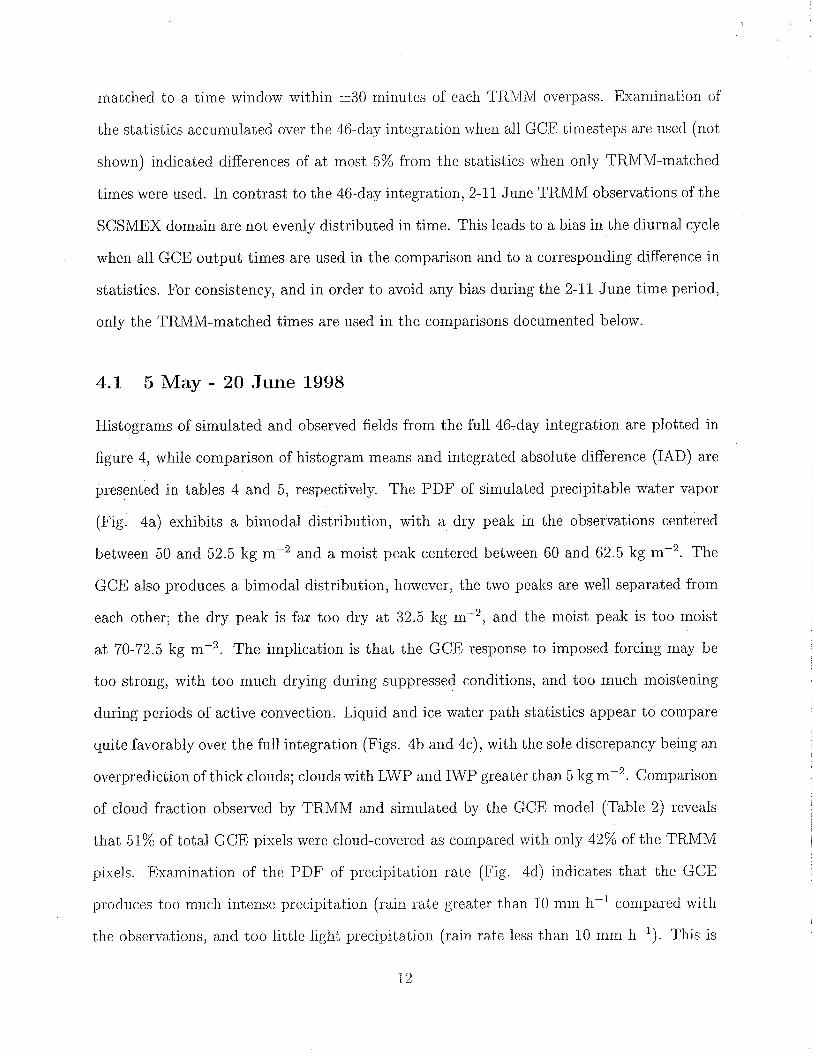
4.1 5 May - 20 June 1998

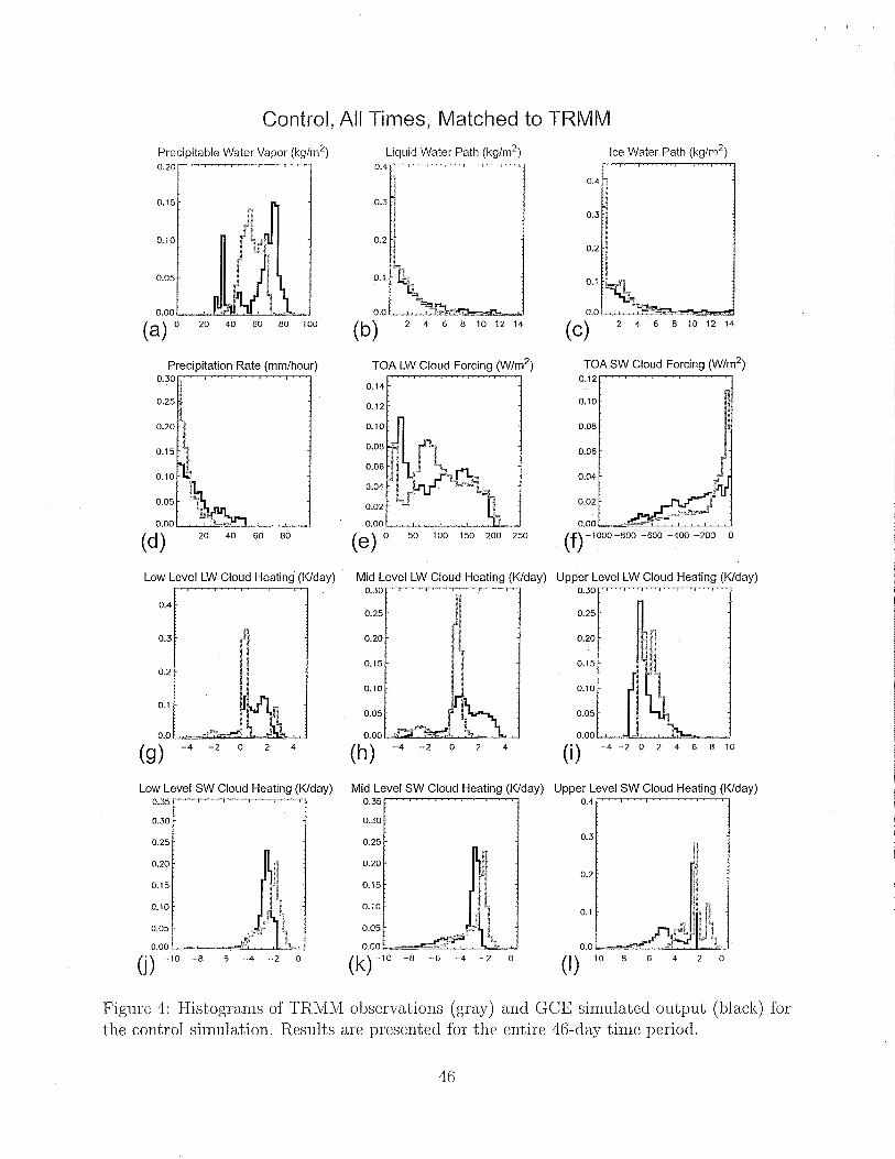
Histograms of simulated and observed fields from the full 46-day integration are plotted in

figure 4, while comparison of histogram means and integrated absolute difference (IAD) are

presented in tables 4 and 5, respectively. The PDF of simulated precipitable water vapor

(Fig. 4a) exhibits a bimodal distribution, with a dry peak in the observations centered

between 50 and 52.5 kg m-2 and a moist peak centered between 60 and 62.5 kg m-2. The

GCE also produces a bimodal distribution, ho-cvever, the two peaks are well separated from

each other; the dry peak is far too dry at 32.5 kg m-2, and the moist peak is too moist

a t 70-72.5 kg mP2. The implication is that the GCE response to imposed forcing may be

too strong, with too much drying during suppressed conditions, and too much moistening

during periods of active convection. Liquid and ice water path statistics appear t o compare

quite favorably over the full integration (Figs. 4b and 4c), with the sole discrepancy being an

overprediction of thick clouds; clouds with LWP and IWP greater than 5 kg m-2. Comparison

of cloud fraction observed by TRMM and simulated by the GCE model (Table 2) reveals

that 51% of total GCE pixels were cloud-covered as conipared with only 42% of the TRMM

pixels. Examination of the PDF of precipitation rate (Fig. 4d) indicates that the GCE

produces too much intense precipitation (rain rate greater than 10 mm h-I compared with

the observations, and too little light precipitation (rain rate less than 10 mm h-I). This is

reflected in the fact that only 5% of the GCE pixels had a precipitation rate greater than

the assumed 1 mm h-' detection threshold as compared with 13% of TRMrVI pixels (Table

2).

PWV, LWP, IWP, and precipitation serve as effective illustrations of the utility of both

the mean and integrated absolute difference in comparing observed and simulated distribu-

tions. In particular, comparison of the means of retrieved and simulated PWV indicate a

relatively close fit between the two distributions, as there is approximately a 10% difference

in means. By contrast, the integrated absolute difference between the two PDFs is 1.28;

a greater than 100% disagreement between the PDFs, indicating that there are significant

differences in the structure of the two histograms. The LWP, IWP, and precipitation rate

histograms exhibit very different means, but the IAD is quite low (less than 0.1 for LWP

and IWP, and less than 0.4 for precipitation rate); an indication that though the overall

structure of the PDFs agrees quite well, there is an error due to sliewness. In general, the

combination of comparable means with large (>1.0) IAD indicates either a misrepresentation

of the dispersion or multiple modes in the observed or simulated PDF. By contrast, if the

IAD is low (< 0.5), but the mean is displaced (as in LWP, IWP, and precipitation rate),

it is an indication that the general structure of the PDF is well-represented, but that the

skewness is not properly represented in the simulated PDF.

The effects of clouds on radiation can be assessed through subtraction of the clear-sky

from all-sky radiative fluxes and heating rates; the resulting quantities are hereafter referred

to as cloud radiative forcing and cloud-aSfected heating rates, respectively.2 Examination

of the cloud radiative forcing (Figs. 4e and 4f) reveals an overprediction of longwave and

shortwave cloud forcing in the GCE simulations; the GCE LW cloud forcing histogram has

two peaks, as in the observations, however, both the low and high peaks are biased toward

2Subtraction of clear-sky fluxes a,nd heating rates serves to filter any bias in the comparison that might be due to use of temperature, water vapor, a,nd gaseous absorption profiles in the TRMM retrievals that differ from those simulated by the model. since the veracity of simulated water vapor ca,n be assessed through comparison of GCE and TRMWI PWV, and since it is the cloud effect on the radiation field that is the focus of the use of a CRM in a MMF, comparison of only the cloud-affected component of fluxes and heating rates is appropriate in this context.

large absolute values of radiative forcing. The peak in the simulated shortwave cloud forcing

is located in the range between -0 to -25 W m-2 , ~vhich is close to the observed -25 to -50

mP2, but the model produces too many instances of large negative shortwave cloud radiative

forcing relative to the observations. Both long and shortwave results are consistent with

overprediction of thick clouds in the GCE, and cloud-affected heating rates follow suit. In

particular, at low levels (Fig. 4g), the GCE PDF is missing the enhanced longwave cloud-

induced cooling, and produces cloudy heating that is too weak by approximately 1.0-1.5 K

d-l. At mid-levels (Fig. 4h), the GCE approximately reproduces the observed histogram

of longwave cooling, but overpredicts cloudy heating, while at high levels (Fig. 4i), the

GCE exhibits a bias toward greater cooling than in the observations. The lack of low-level

longwave cooling is consistent with underprediction of low cloud under otherwise clear skies;

in the case of low cloud under high cloud, cloudy cooling is reduced. Underprediction of

mid-level cloudy cooling is consistent with the presence oT too much high cloud in the GCE,

as most of the midlevel cloud tends to also be associated with the presence of high cloud

(not shown). Simulated shortwave cloud-affected heating rates are biased toward too much

cooling a t all levels, indicating an overprediction of shortwave reflection and consequently

clouds that are too optically thick in the visible. It is interesting to note that, although

the form of the PDFs for low and mid-level cloudy heating are quite similar (Figs. 4k and

41), the PDF of simulated shortwave cloudy heating a t upper levels appears to be missing a

distinct mode at small cooling rates. This, combined with results from low and mid levels

provides a further indication that simulated clouds are too thick relative to those that are

observed.

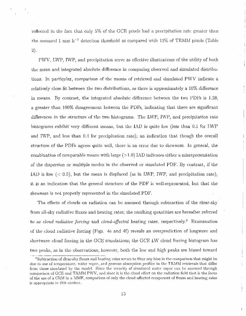
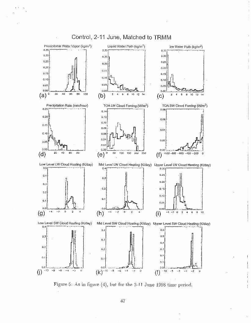
4.2 2-11 June 1998

A comparison of histograms of observed fields from TRMM with GCE output over the 2-

I1 June time period is presented in figure 5. Though a double peak in the PWV field is

still clearly visible in the TRMM observations, the moist mode located between 60-65 kg

mP2 is now the primary one. By contrast, the GCE PkVV has only a single primary peak,

located at 70-75 kg m-2. Comparison of precipitable water vapor from the June time period

with PWV from the entire integration indicates that the peak PWV for the June case is

collocated with the GCE moist mode in the full integration, and that it is still biased moist

compared with the TRMM retrievals. This is reflected in both the mean and IAD; mean

simulated PWV is now significantly different from the retrievals, while the IAD indicates

a disagreement of nearly 100% (IAD = 2.0)./ Compared with the full integration, the June

case exhibits relatively greater departures from TRMM in the liquid and ice water paths;

both simulated LWP and IWP are missing the secondary peak a t LWP of 1.5-2.0 kg m-2

and IWP of 2.0-2.5 kg md2, and both exhibit more occurrences of LWP and IWP greater

than 5 kg mP2 compared with the observations. The histogram mean and IAD again reflect

an increased departure from observations in the 2-11 June case; IAD, in particular, is twice

that computed for histograms over the full 46-day period. In comparing simulated and

observed LWP and IWP, it should be noted that the differences in the means are quite small

relative to the range of simulated values, and that the IAD values reflect a less than 10%

departure from observations for the June case, and less than 5% departure for the full 46-

day period. By contrast, the difference in mean precipitation rate reflects a significant shift

toward higher rain rates in the model, and IAD values indicate a greater than 25% difference

in the PDFs for 2-11 June; an indication that, though the integrated condensate mass may

be well-represented in the GCE, the convection is too intense.

LW cloud radiative forcing in the GCE exhibits a nearly flat histogram from 30-200

W mW2, while the TRMM retrievals pealc noticeably at around 80 W m-2, with a steady

decrease to 200 W m-2. Comparison of simulated and retrieved shortwave cloud radiative

forcing again indicates a preponderance of highly reflective cloud in the GCE model, as

the peak a t low values is much reduced in the GCE, and the simulated PDF exhibits a

pronounced mode at cloud radiative forcing values less tliaii -400 W m-2. By contrast, the

observations exhibit a sharp decrease in the occurrence of shortwave cloud radiative forcing

less than -100 W m-2 and almost zero occurrence of values less than -400 14T m-'. Longwave

cloud affected heating rates exhibit the structures that are similar to those in the long-term

integration, though there is a relatively greater bias toward higher longwave heating at low

and middle levels, and toward smaller heating and larger cooling at upper levels. Shortwave

cloud-affected heating in the model is, as in the long-term integration, biased toward stronger

rates of cooling, though it is interesting to note that the PDFs in the June case are uniformly

narrower than in the 46-day period. In addition, the secondary and tertiary modes in the

observed upper-level shortwave cloudy heating are greatly diminished relative to the full time

period. This is most likely a reflection of the fact that the active phase of the monsoon is

characterized by cirrus anvils in the domain with far fewer middle and low clouds and less

thin cirrus.

The general picture that emerges from comparison of the control GCE simulation with

TRMM retrievals is a model that responds too vigorously to the imposed large-scale forcing,

accumulating too much moisture and producing too much cloud cover during convective

phases, and overdrying the atmosphere and suppressing clouds during monsoon break peri-

ods. Evidence for this is provided in figure 6, in which the daily mean precipitable water

vapor timeseries is plotted from the GCE control run, the TRMM retrievals, and the SC-

SMEX forcing dataset. From this plot, i t can be noted that, though the PWV in the forcing

dataset is consistently higher than that in the TRMM retrievals by a few kg m-2, it tracks

the observed temporal changes in integrated water vapor with great fidelity. In contrast, the

GCE simulated water vapor decreases dramatically early in the time period, and increases

unrealistically in the latter half. I t is interesting to note that, despite the model's problems

simulating the observed distribution of water vapor, the distribution of integrated liquid and

ice cloud mass is generally well-simulated by the GCE, indicating that the cloud microphys-

ical scheme is producing physically realistic clouds. The fact that the precipitation rate is

generally overpredicted compared with observations indicates overactive convection in the

model, while the discrepancies in the cloudy fluxes and heating rates can be explained by

noting that, in spite of the fact that LWP and IWP compare favorably with observations,

there is simply too much cloud cover in the model. The frequency of occurrence of cloudy

pixels is nearly 10% and 20% greater in the model as compared with TRMM observations

for the 46-day and 2-11 June time periods, respectively (Tables 2 and 3).

5 Sensitivity Experiments

Having determined that clouds and water vapor tend to be overpredicted in the control

version of the GCE used in the NASA Goddard MMF, with concomitant effects on the

cloud-affected radiation, sensitivity tests are now performed to assess whether the discrep-

ancies between simulated and observed fields can be traced to the specifics of the model grid

configuration, uncertainties in the cloud microphysical parameterization, or a combination

of both. In the interest of brevity, results are presented only for the 2-11 June case; this

allows identification of the sources of model error that are more directly associated with

post-monsoon onset convection. Two sets of experiments are performed; one in which the

model grid spacing and domain size are modified, and another in which assumptions in the

GCE cloud microphysical parameterization that govern the ice particle size distribution are

changed. The first set of comparisons is aimed at determining whether the differences be-

tween GCE simulated clouds, precipitation, and radiation are due t o coarse grid spacing

and/or a small horizontal domain. Specifically, if changes in domain size can be shown to

improve simulation results, this will be an indication that connection of CRM domains across

GCNI grid cells may lead to an improvement in modeled clouds and precipitation. The sec-

ond set of comparisons is designed t o obtain an order of magnitude estimate of the sensitivity

of CRM simulations in the MMF framework to changes in the assumptions contained in the

GCE cloud microphysical parameterization. If the sensitivity to changes in cloud microphys-

ical parameters is large, this result will provide motivation to further quantify and mitigate

uncertainty in these parameters.

5.1 Grid Size and Spacing

In the cloud resolving modeling community, four kilometer grid spacing is generally accepted

as an upper limit to what may legitimately be called "cloud resolving" (Weisman et al. 1997);

at grid lengths greater than four ltilometers, it is assumed that some manner of subgrid

cumulus parameterization will be necessary to represent convection in the model.3 Since

the CRMs used in current MMFs employ a four kilometer grid spacing, it is appropriate

to consider whether the CRM results presented in this study are sensitive to changes in

grid spacing. To this end, an experiment is performed in which the model grid spacing

is halved to two kilometers (hereafter, 2KM) while the model domain is held fixed at 256

kilometers. While many studies have documented a sensitivity of simulations of cumulus

cloud structure to changes in grid spacing, the role of mesoscale circulations in the evolution

of deep convective systems, particularly those that form in the presence of vertical shear,

has also been well documented (Fovell and Ogura 1989). Arguably, a 256 kilometer cyclic

horizontal domain may be too small to allow development of realistic mesoscale circulations,

hence a simulation is performed in which the model grid is extended to 1024 km in length

(hereafter, 1024KM).

Results from 2KM and 1024KM simulations are presented along with TRMM observa-

tions of the 2-11 June time period in figure 7. Comparison of PWV between control, 2KM,

and 1024KM simulations (Fig. 7a) reveals that a change in the grid spacing and grid length

has a slight effect on the increase of moisture in the model. The fact that the 1024KM

simulation more closely matches the TRMM observations than either the 2KM or control is

likely due to a combination of ttvo factors: (1) a larger domain provides a greater area over

tvhich compensating subsidence can act, and (2) in a larger domain, convective systems must

31ndeed, following recent case studies of turbulent structures in convection (Bryan et al. 2003) and vertically propagating gravity waves (Lane and Icnievel 2005), it is now generally agreed that grid spacing on the order of 100 meters is necessary to appropriately resolve deep convection, with even smaller grid spacings required for the realistic simulation of trade-wind cumulus and stratocumulus clouds. Due to computational limitations, MMFs cannot be run with CRM grid spacings much less than 4 kilometers; the two kilometer grid spacing used here is assunled to be marginally computationally feasible.

travel a greater distance before encountering a cyclic boundary. Some sensitivity t o both

grid spacing and length is also observed in the LIVP and IPVP histograms (Figs. 7b and 7c),

however, as indicated in the histograms and IAD values (Table 7), 2KM and 1024KM sim-

ulations provide little improvement over the control. Comparison of cloud fraction between

TRMM, control, 2KM, and 1024KM (Table 3) indicates that the large-domain simulation

produces a total cloud fraction that is more consistent with TRMM observations, while cloud

cover in 2KM is even greater than in the control simulation. Neither simulation produces

a more realistic precipitating fraction than the control; in fact, the large-domain simulation

produces quite sparse precipitation compared with both the control and 2KM. The precipi-

tation rate (Fig. 7d) itself is sensitive to changes in grid geometry, though neither the 2KM

nor the 1024KM simulation provide a clear improvement over the control. The most notable

difference is the reduction in large precipitation rates in 2KM, however, this improvement

is offset by an anomalous increase in the moderate (10-20 m m h-l) rain rates. 1024KI\iI

exhibits precipitation rates that are even larger on average than the control simulation, and

a precipitating fraction that is one third of what is observed by TRMM. Examination of the

longwave radiative forcing (Fig. 7e) indicates that the 2KM simulation appears to provide

a better fit to the observations than either the control or 1024KM, however, the model is

still biased toward longwave forcing values that are too large compared with TRMM. Im-

provement in 2KM over the control may be due to a reduction in the occurrence of large

LWP values and concurrent reduction of liquid cloud longwave absorption. Both simulations

produce a shortwave cloud radiative forcing PDF (Fig. 7f) that is a better match to ob-

servations than the control; specifically, 1024KM exhibits less than 10% difference from the

observed PDF (Table 7), with a marked reduction in the highest shortwave radiative forcing

values. Comparison of the long and shortwave heating rates (Figs. 7g-71) produced by 2KM

and 1024KM with the control simulation reveal only slight differences in the simulated re-

sults, and it appears that changes to grid spacing and domain size do not affect the overall

distribution of low, middle, and high clouds in the model.

Overall, neither an increase in grid resolution nor an increase in grid domain greatly

improves the veracity of simulated results, though comparison of the total IAD values for

each simulation (Table 7) indicates that both experiments provided a slight overall improve-

ment. Comparison of rain rates and cloud fraction appears to indicate that 2KM may more

effectively simulate stratiform rain than the control, but overproduces it-perhaps due to use

of a small model domain. In contrast, the large domain of 1024KIVI produces improved cloud

fraction, but, as in the control, generates too much convective precipitation relative to strat-

iform. Because recent studies have indicated that grid spacing of less than 500 meters may

be required for proper simulation of deep convection (Bryan et al. 2003, W. Cotton, personal

communication), an experiment was performed in which the grid spacing was reduced to 250

m (results not shown). This simulation produced results that were generally comparable to

those of the 2KM run, with the exception of the shortwave cloud radiative forcing, which

exhibited a significant bias toward large values.

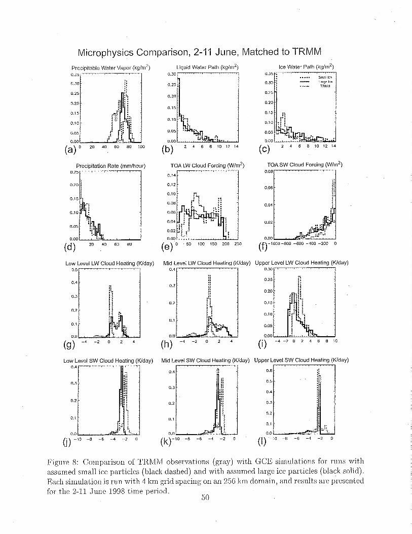
5.2 Sensitivity Experiments: Cloud Microphysical Parameters

As was noted in section 3, the particle size distribution of precipitating ice species (snow

and graupel) in the GCE cloud microphysical scheme is assumed to be exponential, with the

number of particles of a given diameter D parameterized for condensate species x as

where fh, is the slope-intercept and the slope Ax can be written

where p, is the particle density. In addition, the fall velocity of precipitating particles is

typically expressed as a power relationship (Mitchell 1996)

Note that a,, b,, No, and p, are constant parameters that must be specified in advance.

These parameters, along with assumed-constant collision/collection efficiencies for the in-

teractions between each pair of species, govern to some extent the properties of clouds,

precipitation, and water vapor simulated by the model. To rigorously assess the sensitivity

of the full set of cloud microphysical parameters used in the GCE, each parameter should be

systematically varied while the others are held constant. Though such an exercise is beyond

the scope of this study, it is useful to obtain an order of magnitude estimate of the effect of

changes to these parameters on simulated output. Hence, in this section the uncertainty of

simulated output to changes in cloud microphysical parameters is estimated by considering

two scenarios; one in which precipitating ice particles are uniformly assumed to be small

compared to the control, and one in which ice particles are assumed to be large. In the

small-ice case (hereafter SMICE), the slope intercepts of the snow and graupel ice particle

size distributions are increased, while the collection efficiencies and fall speed parameters

are decreased. In the large-ice case (hereafter LGICE), the opposite is done; collection effi-

ciencies and fall speed parameters are increased, while snow and graupel slope intercepts are

decreased. In each experiment, perturbations are applied within the range of values reported

in the literature (Locatelli and Hobbs 1974, Mitchell 1996), and results are compared with

TRMM retrievals as in sections 4 and 5.1.

Histograms of fields output from both SMICE and LGICE simulations are presented in

figure 8. The PDFs of precipitable water vapor from each case (Fig. 8a) indicate that, in

contrast to the domain and grid spacing perturbation experiments, changes to ice microphys-

ical parameters have a relatively large effect on the accumulated water vapor. The SMICE

simulation exhibits an even larger moist bias than the control, with mean PWV of 75.56 l<g

n ~ - ~ and IAD of 1.90, while the LGICE simulation produces an improved match to TRMM

retrievals, with mean PWV of 70.82 kg m-2 and IAD of 1.60 (Table 7). I t is interesting that

21

both perturbation experiments yield better fits to the observed PDFs of LIVP, IWP, and

precipitation rate than the control, though close inspection of the I\VP histograms reveals

a tendency toward thicker ice clouds in the LGICE case as compared to SMICE (Fig. 8d).

Examination of the LW cloud radiative forcing (Fig. 8e) reveals that the SMICE simulation

yields nearly identical results as in the control, while the LGICE run produces a better fit

a t the larger values. This comes a t the expense of a poorer fit to.the observed PDF at small

values; hence the IAD is nearly identical between SMICE and LGICE runs. Both SMICE

and LGICE simulations produce a nearly identical tail in the shortwave radiative forcing

(Fig. Sf), though the LGICE simulation produces a closer fit at smaller values, and thus the

overall IAD is smaller (Table 7). I t is interesting to note that both SMICE and LGICE pro-

duce a better fit to the observations than the control, primarily through a visible reduction

in the number of SPV radiative forcing values less than -400 W mP2. This is reflected in the

fact that the means of SMICE and LGICE simulations are closer to that of TRMM, and the

IAD values are smaller than in the control. In contrast to the cloud, precipitation, vapor,

and radiative forcing, the cloud-affected heating rates do not differ much between the con-

trol simulation, SMICE, and LGICE. Aside from a slightly better agreement in the mid-level

shortwave radiative heating for LGICE, the histograms are nearly identical, as are the means

and IAD values. As was the case for the control and grid sensitivity experiments, changes

to cloud microphysical parameters appear not to affect the simulated distribution of low,

middle, and high clouds, nor to mitigate the biases in cloud-affected radiative heating. The

fact that the cloud fraction was similar between SMICE, LGICE, and control indicates that

a combination of a larger grid with proper specification of cloud microphysical parameters

may be needed for improved simulation of clouds and precipitation.

.6 Discussion

6.1 Integrated Absolute Difference

Though most of the results presented in sections 4 and 5 involved visual inspection of PDF

structures, the utility of the mean and integrated absolute difference as quantitative metrics

in the statistical comparison was also clearly demonstrated. Use of these statistics becomes

increasingly valuable as the work transitions from comparison t o assimilation; in particular,

given appropriate specification of error statistics, mean and IAD provide different pieces of

information that together can be used t o constrain uncertainty in the model. The primary

drawback to the use of any integrated measure of difference between histograms lies in

the discretization of the histogram into bins; if bin sizes are defined too small, spurious

differences in histograms over small ranges will lead to consistently large IAD. By contrast,

if bin sizes are set too large, the comparison may neglect important characteristics of either

the observed or simulated PDF; e.g., secondary modes. The method that perhaps makes the

most intuitive sense is to let the bin size depend on the error in the observations themselves.

In this way, a measure of the observation uncertainty explicitly enters the process, and there

is less chance that there will be noise in the comparison. In addition, it is unlikely that

statistically significant structures can exist in the observed PDFs a t scales that are smaller

than, or comparable to the error magnitude.

6.2 CRM Feedback to the Large Scales

This study has considered the effect of changes in grid configuration and cloud microphysical

parameters on the simulated histograms, however, an equally important consideration is the

feedback of the CRM temperature and moisture tendencies to the large scale. This feedback

can be computed following I<hairoutdinov et al. (2005) as

-+I where QLs is the variable of interest on the GCM grid and is the accumulated CRM

tendency over the GCM timestep AtLs. In the current case, no feedback from the CRM to

the large scales is allowed, and the CRM "forcing" is computed a t half-hour intervals as

where [%Itotai is the total change in @ over the half-hour interval, and [%ILS is the tendency

of @ obtained from the observed large-scale forcing fields.

Total domain mean temperature and water vapor feedbacks are computed from equation

(5) over the 2-11 June time period for the each simulation. The CRM temperature response

(Fig. 9a) exhibits a structure that is nearly identical across all model configurations, with

heating maximized in the middle troposphere and cooling observed near the surface and

above 15 km. The vertical structure closely resembles superposition of a strong convective

heating profile on a much weaker stratiform mode, and reinforces the notion that the model

generates too much convective precipitation relative to stratiform. Cooling above 15 km,

combined with heating between 12 and 15 km is consistent with the existence of thick cirrus

anvils in all simulations. I t is interesting to note that differences in the temperature feedback

are greatest in the upper troposphere, a reflection of the vertically integrated effect of changes

in cloud properties and distribution between different simulations. Though comparison with

the temperature feedback reveals greater variability in the water vapor response, the CRM

water vapor feedback (Fig. 9b) exhibits moistening in the lower and middle troposphere in

all simulations. The moistening is greatest below 5 km, where evaporation of precipitation

is occurring, and it can be seen that differences between simulations generally reflect the

differences in the mean precipitable water vapor during the June time period (Table 6).

6.3 Role of Large Scale Forcing

The results presented in sections 4 and 5 above indicate that the GCE appears to produce an

overactive response to large scale forcing, generating too much cloud and water vapor during

periods of active convection. Though the large-scale forcing datasets used in this study have

been extensively evaluated, and comparisons between PWV derived from the analysis and

from TRMM demonstrate close agreement, i t is fitting t o examine how simulation results

might change if the forcing were reduced. In this case, it is assumed that all sources of

forcing are overestimated, and a constant correction factor is applied in the model equations

so that the forcing magnitude is reduced to 80%. The control simulation is then re-run

with the adjusted forcing, and fields are compared with the original control simulation. The

results of reducing the large-scale forcing are in general comparable with the results from the

unadjusted control simulation, with a few notable exceptions. In particular, the simulated

precipitable water vapor, precipitation rate, LWP, and IWP (Fig. 10) are decreased relative

t o the control to values that are comparable with that observed in the LGICE simulation

(Fig. 8). By contrast, the cloud-affected long and shortwave fluxes and heating rates are

unaffected (results not shown). The implication is that , while a reduction in forcing appears

t o have led to a reduction in convective intensity, as measured by the precipitation rate,

cloud thickness, and accumulation of water vapor, it does not appear that a bias in the large

scale forcing fields is necessarily the reason for the discrepancies observed between simulation

and observations.

7 Summary and Conclusions

In this study, clouds, precipitation, and long and shortwave radiation simulated by a cloud-

resolving model were evaluated against retrievals from TRMM. The two-dimensional NASA

Godclard cumulus ensemble cloud resolving model was run in an identical configuration to

that used in the NASA Goddard multiscale modeling framework with a relatively small

Cotton 2004) has recently been included in the GCE model, and the radiative transfer of

Gabriel et al. (2001) and Stephens et al. (2001) has also been implemented to provide more

accurate treatment of the interaction of radiation with the RAMS cloud and ice condensate

s'pecies. Tests of the RAMS microphysical scheme and Gabriel-Stephens radiation code are

underway, and comparison of simulation results with TRNIM observations is left for a future

study. Finally, i t is reasonable to expect that the role of cloud microphysical parameters

might change when CRM simulations are run over different geographical regions and for

different seasons. Further comparison of CRM results vs. observations will be necessary to

determine whether this is, indeed, the case.

Acknowledgments

The authors wish to thank Paul Ciesielski for his instructive comments regarding the SC-

SMEX forcing dataset. Chung-Lin Shie provided extensive assistance with configuring and

running the GCE model, while Steve Lang offered enlightening discussions of the particulars

of the GCE cloud microphysical scheme. This work was funded by NASA NMP contract

NAS1-00072 and by NASA Energy and Water Cycle Sponsored (NEWS) research grant

NNG06GC46G. W.-K. Tao wishes to thank Dr. D. Anderson a t NASA headquarters for

his support under the Cloud Modeling and Analysis Initiative (CMAI) program. Tao also

wishes to thank Dr. R. Kakar for supporting the GCE model development and improvement

through PMM.

References

Arakatva, A., and W. H. Schubert, 1974: Interaction of a cumulus cloud ensemble with the

large-scale environment. Part I. J. Atmos. Sci., 31, 674-701.

P I 2004: The cumulus parameterization problem: past, present, and future. J. Cli-

23

mate, 17, 2493-2525.

Bony, S., R. Colman, V. M. Kattsov, R. P. Allan, C. S. Bretherton, J.-L. Dufresne, A.

Hall, S. Hallegatte, M. M. Holland, W. Ingra,m, D. A. Randall, B. J . Soden, G. Tselioudis,

and M. J . Webb, 2006: How well do we understand and evaluate climate change feedback

processes? J. Climate, 19, 3445-3482.

Bryan, G. H., J. C. Wyngaard, and J. M. Fritsch, 2003: Resolution requirements for the

simulation of deep moist convection. Mon. Wea. Rev., 131, 2394-2416.

Chou, M.-D., and L. Kouvaris, 1991: Calculations of transmission functions in the IR COa

and O3 bands. J. Geophys. Res., 96, 9003-9012.

-, W. Ridgway, and M.-H. Yan, 1995: Parameterizations for water vapor IR radia-

tive transfer in both the middle and lower atmospheres. J. Atmos. Sci., 52, 1159-1167.

-, and M. J. Suarez, 1999: A shortwave radiation parameterization for atmospheric

studies. 15, NASA/TM-104606, 40 pp.

-7 K.-T. Lee, S.-C. Tsay, and Q. Fu, 1999: Parameterization for cloud longwave scat-

tering for use in atmospheric models. J. Clim., 12, 159-169.

Cooper, S. J., T. S. L'Ecuyer, and G. L. Stephens, 2003: The impact of explicit cloud bound-

ary information on ice cloud microphysical property retrievals from infrared radiances. J.

Geophys. Res., 108, DOI: 10.1029/2002 JD002611.

Cotton, \V. R., R. A. Pielke Sr., R. L. Walko, G. E. Liston, C. J. Tremback, H. Jiang,

29

Kratz, D. P., M.-D. Chou, &I.-H. Yan, and C.-H. Ho, 1998: Minor trace gas radiative forcing

calculations using the k-distribution method with one-parameter scaling. J. Geophys. Res.,

103, 31647-31656.

Kummerow, C. and Co-Authors, 2000: The status of the Tropical Rainfall Measuring Mis-

sion (TRMM) after two years i'n orbit. J. Appl. Meteor., 39, 1965-1982.

Lang, S., W.-K. Tao, R. Cifelli, W. Olson, J. Halverson, S. Rutledge, and J. Simpson,

2007: Improving simulations of convective systems from TRMM LBA: easterly and westerly

regimes. J. Atmos. Sci., In Press.

Lau, K. M., and Coauthors, 2000: A report of the field operations and early results of

the South China Sea Monsoon experiment (SCSMEX). Bull. Amer. Meteor. Soc., 81, 1261-

1270.

LIEcuyer, T . S., and G. L. Stephens, 2002: An uncertainty model for Monte Carlo re-

trieval algorithms: Application to the TRMM observing system. Quart. J. Roy. Meteor.

Soc., 128, 1713-1737.

-, and G. L. Stephens, 2003: The tropical oceanic energy budget from the TRMM

perspective. Part I: Algorithm and uncertainties. J. Climate, 16, 1967-1985.

Lin, Y.-L., R. D. Farley, and H. D. Orville, 1983: Bulk parameterization of the snow field in

a cloud model. J. Climate Appl. Meteor., 22, 1065-1092.

Locatelli, J . D., and P. V. Hobbs, 1974: Fall speeds and masses of solid precipitation parti-

cles. J. Geophys. Res., 79, 2185-2197.

Luo, Z., and G. L. Stephens, 2006: An enhanced convection-wind-evaporation feedback in a

superparameterization GCM (SP-GCM) depiction of the Asian summer monsoon. Geophys.

Res. Lett., 33, L06707, doi:10.1029/2005GL025060.

Meyers, IVI. P., R. L. Walko, J. Y. Harrington, and W. R. Cotton, 1997: New RAMS micro-

physics parameterization. Part 11: the two-moment scheme. Atmos. Res., 45, 3-39.

Mitchell, D. L., 1996: Use of mass- and area-dimensional power laws for determining precip-

itation particle terminal velocities. J. Atmos. Sci., 53, 1710-1723.

Nuss, W. A., and D. W. Titley, 1994: Use of multiquadric interpolation for meteorologi-

cal objective analysis. Mon. Wea. Rev., 122, 1611-1631.

Petch, J. C., and M. E. B. Gray, 2001: Sensitivity studies using a cloud-resolving mode1

simulation of the tropical west Pacific. Q. J. Roy. Met. Soc., 127, 2287-2306.

Randall, D. A., M. Khairoutdinov, A. Araka~va, and W. W. Grabowski, 2003: Breaking

the cloud parameterization deadlock. Bull. Amer. Met. s&., 84, 1547-1564.

Rutledge, S. A., and P. V. Hobbs, 1983: The mesoscale and microscale structure and orga-

nization of clouds and precipitation in midlatitude cyclones. VIII: A model for the "seeder-

feeder" process in warm-frontal rainbands. J. Atmos. Sci., 40, 1185-1206.

-, and P. V. Hobbs, 1984: The mesoscale and microscale structure and organization

of clouds and precipitation in midlatitude cyclones. Part XII: A diagnostic modeling study

of precipitation development in narrow cold frontal rainbands. J. Atmos. Sci., 41, 2949-2972.

Saleeby, S. M., and W. R. Cotton, 2004: A large-droplet mode and prognostic number con-

centration of cloud droplets in the Colorado State University Regional Atmospheric i\/Iodeling

System (RAMS). Part I: module descriptions and supercell test simulations. J. Appl. Me-

teor., 43, 182-195.

Smolarkiewicz, P. K., 1983: A simple positive definite advection scheme with small im-

plicit diffusion. Mon. Wea. Rev., 111, 479-486.

-, 1984: A fully multidimensional positive definite advection transport algorithm with

small implicit diffusion. J. Comput. Phys., 54, 325-362.

-, and W. W. Grabowski, 1990: The multidimensional positive advection transport

algorithm: nonoscillatory option. J. Comput. Phys., 86, 355-375.

Soden, B. J., and I. M. Held, 2006: An assessment of climate feedbacks in coupled ocean-

atmosphere models. J. Climate, 19, 3354-3360.

Soong, S.-T., and Y. Ogura, 1980: Response of trade wind cumuli to large-scale processes.

J. Atmos. Sci., 37, 2036-2050.

-, and W.-K. Tao, 1980: Response of deep tropical clouds to mesoscale processes.

J. Atmos. Sci., 37, 2016-2035.

Stephens, G. L., P. M. Gabriel and P. T. Partain, 2001: Parameterization of Atmospheric

Radiative Transfer. Part I: Validity of Simple Models. J. Atmos. Sci., 48, 3391 - 3409.

Y. C. Sud and G. K. Walker, 1999: Microphysics of clouds with the relaxed Arakawa-

Schubert scheme (McRAS). Part I: Design and evaluation with GATE phase III data. J.

Atmos. Sci., 56, 3196-3220.

Tao, 1V.-K., and Y. Ogura, 1986: A study of the response of deep tropical clouds to mesoscale

processes: Three dimensional numerical experiments. J. Atmos. Sci., 43, 2653-2676.

-, J . Simpson, and M. McCumber,l989: Ice-water saturation adjustment. Mon. Wea.

Rev., 117, 231-235.

-, and J. Simpson, 1993: Goddard Cumulus Ensemble Model. Part I: Model De-

scription. Terrestrial, Atmospheric, and Oceanic Sciences, 4, 35-72.

-7 C.-L. Shie, R. H. Johnson, S. Braun, J . Simpson, and P. E. Ciesielski, 2003a: Con-

vective systems over the South China Sea: cloud-resolving model simulations. J. Atmos.

Sci., 60, 2929-2956.

-7 J . Simpson, D. Baker, S. Braun, M.-D. Chou, B. Ferrier, D. Johnson, A. Khain,

S. Lang, B. Lynn, C.-L. Shie, D. Starr, C.-H. Sui, Y. Wang, and P. Wetzel, 2003b: Micro-

physics, radiation, and surface processes in the Goddard Cumulus Ensemble (GCE) model. A

Special Issue on Non-hydrostatic Mesoscale Modeling, Meteorology and Atmospheric Physics,

82, 97-137.

-7 D. Johnson, C.-L. Shie, and J. Simpson, 2004: The atmospheric energy budget and

large-scale precipitation efficiency of convective systems during TOGA COARE, GATE, SC-

ShlIEX, and ARM: cloud-resolving model simulations. J. Atmos. Sci., 61, 2405-2423.

-, J. Chern, R. Atlas, D. A. Randall, X. Lin, M. F. Khairoutdinov, J.-L. Li, D. E.

Waliser, A. Y. Hou, C. Peters-Lidard, W. Lau, and J. Simpson, 2007: A multi-scale model-

ing system: developments, applications and critical issues. Submitted to J. Geophys. Res.

Tompkins, A. M., 2000: The impact of dimensionality on long-term cloud-resolving model

simulations. Mon. Wea. Rev., 128, 1521-1535.

Wallto, R. L., W. R. Cotton, M. P. Meyers, and J . Y. Harrington, 1995: New RAMS cloud

microphysics parameterization. Part I: the single-moment scheme. Atmos. Res., 38, 29-62.

Weisman, M. L., W. C. Skamarock, and J . B. Klemp, 1997: The resolution dependence

of explicitly modeled convective systems. Mon. Wea. Rev., 125, 527-548.

Zhang, G. J., and N. A. McFarlane, 1995: Sensitivity of climate simulations to the pa-

rameterization of cumulus convection in the Canadian Climate Centre general circulation

model, Atmos. Ocean, 33, 407-446.

List

1 Observations used in the GCE comparison study, along with their units and

error estimates. . . . . . . . . . . . . . . . . . . . . . . . . . . . . . . . . . . 40

Cloudy and precipitating fraction from TRMM and each of the GCE simula-

tions over the entire 46-day integration period. . . . . . . . . . . . . . . . . 40

Cloudy and precipitating fraction from TRMM and each of the GCE simula-

tions over the 2-11 June 1998 time period. . . . . . . . . . . . . . . . . . . . 40

Mean values of each of the simulated and observed fields over the entire 46-day

integration period. . . . . . . . . . . . . . . . . . . . . . . . . . . . . . . . . 41

Integrated absolute difference between PDFs generated from each GCE sim-

ulation and those observed by TRMM over the full 46-day integration. . . . 41

Mean values of each of the simulated and observed fields over the 2-11 June

1998 time period. . . . . . . . . . . . . . . . . . . . . . . . . . . . . . . . . 42

Integrated absolute difference between PDFs generated from each GCE sim-

ulation and those observed by TRMM over the 2-11 June 1998 time period. 42

Table 1: Observations used in the GCE comparison study, along with their units and error estimates.

Observation I Units I Error

Precipitable Water Vapor I k g . m-2 1 10 % Precipitation Rate I rnrn - hr-' 1 25 % Liquid Water Path ( kg - mp2 1 40 %

Ice Water Path I kg - rn-2 f 100 % TOA LW Cloud Forcing I W - m - 2 I 20 % - I I

TOA SW Cloud Forcing I ~ . r n - ~ 1 40 % Three-Layer All-Sky LW and SW

Radiative Cooling/Heating

Three-Layer Clear-Sky LW and SW

Radiative Cooling/Heating

Table 2: Cloudy and precipitating fraction from TRMM and each of the GCE simulations over the entire 46-day integration period.

Table 3: Cloudy and precipitating fraction from TRWIM and each of the GCE simulations over the 2-11 June 1998 time period.

1 TRMM 1 CTRL I SMICE I LGICE I Ax =2 km 1 1000 km I I I I I I I

Cloudy I 0.60 / 0.80 / 0.85 / 0.79 1 0.82 1 0.63

LGICE 0.49 0.05

Cloudy Precipitating

I Precipitating I 0.16 1 0.09 1 0.10 1 0.10 1 0.10 1 0.06 1

CTRL 0.51 0.05

TRMM 0.42 0.13

SMICE 0.54 0.05

Ax =2 km 0.53 0.05

1000 km 0.43 0.04

Table 4: Mean values of each of the simulated and observed fields over the entire 46-day integration period.

I Observation / TRMM CTRL SMICE LGICE Ax =2 km 1000 km /

Table 5: Integrated absolute difference between PDFs generated from each GCE simulation and those observed by TRMM over the full 46-day integration.

/ Observation I CTRL SMICE LGICE Ax =2 lrm 1024 km I

PWV

LWP

IWP

Precip Rate

LW CRF

SW CRF

Low Qlw

Alid Qlw

Upper Qlw

Low QS'CV

Mid Qsw

Upper Qstv

PWV 1 LWP

I IWP

Precip Rate

LW CRF

SW CRF

Low Qlw

Mid Qlw

Upper Qlw

Low QSW

Mid Qsw

Upper Qsw

55.21

0.09

0.14

0.23

94.90

-90.66

0.48

-0.23

0.99

-2.19

-2.74

-2.08

I Total 1 9.00 9.25 8.60 8.96 8.79 1

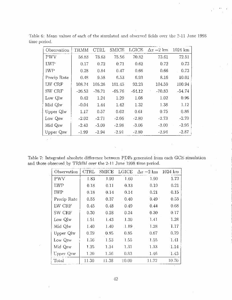
Table 6: Mean values of each of the simulated and observed fields over the 2-11 June 1998 time period.

1 Observation I TRMM CTRL SMICE LGICE Ax -2 ltrn 1024 ltrn 1 P\VV

LWP

IWP

Precip Rate

58.83 73.63 75.56 70.82 73.61 72.51

0.17 0.72 0.71 0.62 0.72 0.73

0.28 0.84 0.47 0.66 0.66 0.73

0.48 9.58 6.53 6.93 8.16 10.01

LW CRF

SW CRF

Low Qlw

Table 7: Integrated absolute difference between PDFs generated from each GCE simulation and those observed-by TRMM over the 2-11 June 1998 time period.

108.74 105.26 101.45 92.23 104.59 100.94

-26.53 -76.71 -65.76 -64.12 -70.83 -54.74

0.42 1.24 1.29 1.08 1.02 0.96

Mid Qlw

Upper Qlw

Low Qsw

Mid Qsw

Upper Qsw

Observation I CTRL SMICE LGICE Az =2 km 1024 k m

-0.04 1.44 1.42 1.32 1.38 1.12

1.17 0.57 0.62 0.61 0.75 0.86

-2.02 -2.71 -2.66 -2.80 -2.73 -2.70

-2.43 -3.00 -2.98 -3.06 -3.00 -2.95

-1.99 -2.94 -2.91 -2.80 -2.94 -2.87

P\VV

LWP

IWP

Precip Rate

LW CRF

SW CRF

Low Qlw

Mid Qlw

Upper Qlw

Low Qsw

Mid QSW

Upper Qs-cv

Total

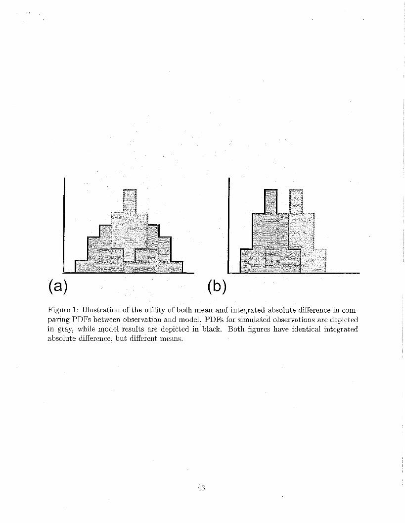
Figure 1: Illustration of the utility of both mean and integrated absolute difference in com- paring PDFs between observation and model. PDFs for simulated observations are depicted in gray, while model results are depicted in black. Both figures have identical integrated absolute difference, but different means.

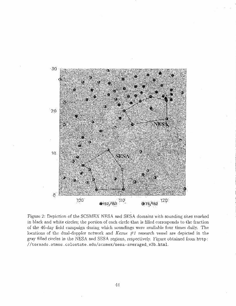
Figure 2: Depiction of the SCSMEX NESA and SESA domains with sounding sites marked in black and white circles; the portion of each circle that is filled corresponds to the fraction of the 46-day field campaign during which soundings were available four times daily. The locations of the dual-doppler network and Kexue #1 research vessel are depicted in the gray filled circles in the NESA and SESA regions, respectively. Figure obtained from http: //tornado.atmos.colostate.edu/scsmex/nesa-averaged~v3b.html.

TRMM Daily Averaged Precipitation and OLR Timeseries 40 300

Figure 3: Depiction of the daily domain-averaged precipitation rate (black) and outgoing longwave radiative flux (gray) retrieved from TRMM over the 46-day SCSMEX intensive observation period.

Control, All Times, Matched to TRMM Precipitable Water Vapor (kg/m2) Liquid Water Path (kg/m2) ice Water Path (kg/rn2) 0.20

0.4

0.15 0.3

0.10 0.2 0.2

0.05 0.1

0.00 0.0 0.0

Precipitation Rate (rnrnlhour) TOA LW Cloud Forcing (w/rn2) TOA SW Cloud Forcing (w/rn2) 0.30

0.14

0.25 0.12

0.20 0.10

0.15 0.08

0.06 0.10

0.04

0.05 0.02

0.00 0.00

(d) 20 40 60 80 50 100 150 200 250 1000-800 -600 -400 -200 0

Low Level LW Cloud Heating (Wday)

0.4 7 4 Mid Level LW Cloud Heating (Wday) Upper Level LW Cloud Heating (Wday)

0.30 -j

(h) -" -' 0 2 4 - 4 - 2 0 2 4 6 8 10

Low Level SW Cloud Heat~ng (Wday) Mid Level SW Cloud Heating (Wday) Upper Level SW Cloud Heating (Klday) 0.35

0 20

0.15 0.15

0 10 0 10 0 1

0 05

(j) -10 -8 -6 -4 -2 0 ( k ) - 1 0 -8 -6 -4 -2 0 (1) -10 -8 -6 -4 -2 0

Figure 4: Histograms of TRMM observations (gray) and GCE simulated output (black) for the control simulation. Results are presented for the entire 46-day time period.

Control, 2-1 1 June, Matched to TRMM Precipitable Water Vapor (kg/m2)

0.30

Liquid Water Path (kg/rn2) 0.30 r-1 Ice Water Path (kg/rn2)

0.35 F-'---"--"-mj

Precipitation Rate (mmlhour) TOA LW Cloud Forcing (w/m2) TOA SW Cloud Forcing (w/m2) 0.25 0.08

0.14

0.12 0.06

0.10

0.08 0.04

0.10 0.06

0.04 0.02

0.02

0.00 0.00 0.00

Low Level LW Cloud Heating (Wday) Mid Level LW Cloud Heating (Wday) Upper Level LW Cloud Heating (Wday) 0.30

0.25

0.20

0.15

0.10

0.05

0.00

(i> - 4 - 2 0 2 4 6 8 10

Low Level SW Cloud Heating (Wday) Mid Level SW Cloud Heating (Klday) Upper Level SW Cloud Heating (Wday)

Figure 5: As in figure (4), but for the 2-11 June 1998 time period.

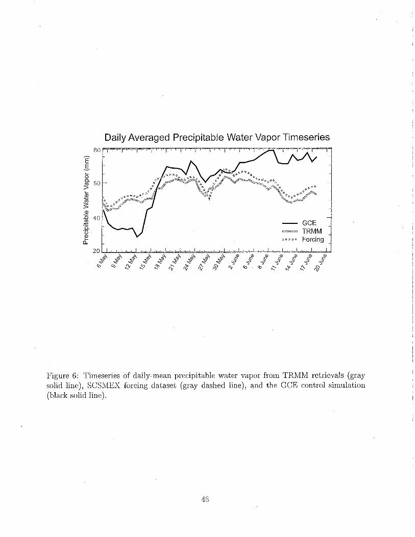
Daily Averaged Precipitable Water Vapor Timeseries

- TRMM

Figure 6: Timeseries of daily-mean precipitable water vapor from TRMM retrievals (gray solid line), SCSMEX forcing dataset (gray dashed line), and the GCE control simulation (black solid line).

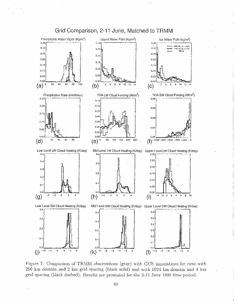
Grid Comparison, 2-1 1 June, Matched to TRMM Precipitable Water Vapor (kg/m2) Liquid Water Path (kg/m2) Ice Water Path (kg/m2)

0.30 0.35

0.25 0.30 - 256km,dx=Zkm = TREAEJ

0.20 0.25

0.20 0.15

0.15

0.10 0.10

0.05 0.05

0.00 0.00 20 40 60 80 100 (b) 2 4 6 8 1 0 1 2 1 4 2 4 6 8 10 12 14

Precipitation Rate (rnrnlhour) TOA LW Cloud Forcing (w/rn2) TOA SW Cloud Forcing (w/rn2) 0.25 0.08

0.20 0.06

0.15

0.04

0.10

0.05 0.02

0.00 0.00

(d) 20 40 60 80

(e) 50 100 150 200 250

( f ) - 1000 -800 -600 -400 -200 0

Low Level LW Cloud Heating (Wday) Mid Level LW Cloud Heating (Wday) Upper Level LW Cloud Heating (Wday) 0.4 0.30

0.25 0.3

0.20

0.2 0.15

0.10 0.1

0.05

0.0 0.00 0 2 4

(h) -4 -2 O (0 - 4 - 2 0 2 4 6 8 1 0

Low Level SW Cloud Heating (Wday) Mid Level SW Cloud Heating (Klday) Upper Level SW Cloud Heating (Wday) :rfl 0.3

0.2

8 0.1 : "

: 1 0.0 # e (j) -10 -8 -6 -4 -2 0 (1) -10 -8 -6 -4 -2 0

Figure 7: Comparison of TRMM observations (gray) with GCE simulations for runs with 256 km domain and 2 km grid spacing (blacli solid) and with 1024 km domain and 4 kni grid spacing (blacli dashed). Results are presented for the 2-11 June 1998 time period.

Microphysics Comparison, 2-1 1 June, Matched to TRMM

Precipitable Water Vapor (kg/m2) 0.35 1-4

Liquid Water Path (kg/m2) 0.301"'1""'' """"'"'""I

Ice Water Path (kg/m2)

- Large Ice

Precipitation Rate (mmlhour) TOA LW Cloud Forcing (w/m2) TOA SW Cloud Forcing (w/m2)

0.04

0.02

0.00

(d) 20 40 60 80 50 100 150 200 250 1000 -800 -600 -400 -200 0

Low Level LW Cloud Heating (Wday) Mid Level LW Cloud Heating (Wday) Upper Level LW Cloud Heating (Wday) 0.4 0.30

0.25 0.3

0.20

0.2 0.15

0.10 0.1

0.05

0.0 0.00 2 4 (0 -4-20 2 4 6 8 10

Low Level SW Cloud Heating (Wday) Mid Level SW Cloud Heating (Wday) Upper Level SW Cloud Heating (Wday)

0.4

0.3

0.2

0.1

0.0 (j) -10 -8 -6 -4 -2 0 (k)-10 -8 -6 -4 -2 0

Figure 8: Comparison of TRMM observations (gray) with GCE sinlulations for runs with assumed small ice particles (black dashed) and with assumed large ice particles (black solid). Each simulation is run with 4 km grid spacing on an 256 ltm domain, and results are presented for the 2-11 June 1998 time period.

5 0

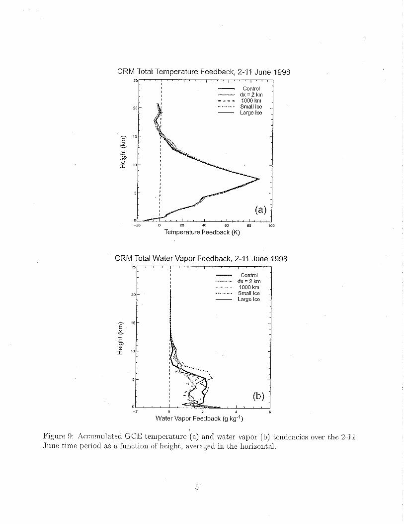
CRM Total Temperature Feedback, 2-1 1 June 1998 2 5 ~ 8 6 0 ~ ~ ~ ~ ~ s 8 ~ ~ ~ ~ ~ ~ ~ ~ ~ ~ ~ ~ ~ ~

t I I - Control - I I - dx=2krn - I - - - - 1000 km -

-,.,...,. Small Ice -

- 15 -

I

I

1 1 ~ 1 1 1 1 1 1 1 1 1 1 1 1 1

-20 0 20 40 60 80 100

Temperature Feedback (K)

CRM Total Water Vapor Feedback, 2-11 June 1998 2 5 [ " ' 1 ~ ~ ~ { ~ ~ ~ 1 a s * l

-2 0 2 4 6

Water Vapor Feedback (g kg-')

Figure 9: Accumulated GCE temperature (a) and water vapor (b) tendencies over the 2-11 June time period as a function of height, averaged in the horizontal.

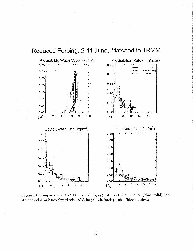
Reduced Forcing, 2-11 June, Matched to TRMM

Precipitable Water Vapor (kg/m2) 0.35 7 1

Precipitation Rate (mm/hour) . L ~ ' . " l . . . l " ' " " - Control - - - - 80% Forcing

0.20

0.1 5

Liquid Water Path (kg/m2)

0.25

Ice Water Path (kg/m2)

Figure 10: Comparison of TRMM retrievals (gray) with control simulation (black solid) and the control simulation forced with 80% large scale forcing fields (black dashed).