Ville Leppälä Evaluation of a Small Brushless Direct Current Motor in an Opto-Mechanical Positioning Application

Thesis of diploma given in for the degree of Master of Science in Technology Espoo 3rd of January 2019 Supervisor: Professor Kari Tammi Instructor: MSc. Klaus Melakari

Aalto-yliopisto, PL 11000, 00076 AALTO www.aalto.fi

Diplomityön tiivistelmä Tekijä Ville Leppälä Työn nimi Harjattoman tasavirtamoottorin arviointi opto-mekaanisessa paikkasää-tösovelluksessa Koulutusohjelma Mechanical Engineering Pääaine Mechanical Engineering

Työn valvoja Professori Kari Tammi Työn ohjaaja Diplomi-insinööri Klaus Melakari Päivämäärä 03.01.2019 Sivumäärä 54 Kieli englanti

Tiivistelmä Tämän diplomityön tarkoituksena on arvioida pienikokoisen harjattoman tasavirtamootto-rin soveltuvuutta opto-mekaaniseen paikkasäätösovellukseen. Harjattomat tasavirtamoot-torit ovat elektronisesti ohjattuja moottoreita, joissa ilmavälin magneettivuo luodaan kes-tomagneeteilla. Moottorille syötetään virtaa taajuusmuuttajalta, joka muodostaa halutun-laisen vaihtovirran jokaiselle moottorin vaiheelle. Syötettävää virtaa ohjataan mootto-rinohjaimelta määritettyjen vääntö-, nopeus- ja paikkavaatimusten perusteella. Harjatto-man DC-moottorin edut verrattuna perinteiseen harjalliseen DC-moottoriin ovat hyvä teho-paino-suhde, hiljainen käyntiääni ja pitkä käyttöikä. Diplomityön tavoitteena on kartoittaa kyseisen moottorityypin suorituskyky paikkasää-dössä ja tutkia keinoja saavuttaa haluttu taso. Alan tutkimuksessa ja kirjallisuudessa tun-nettuja suorituskykyisiä säätömenetelmiä ja laite- sekä komponenttikokoonpanoja on koostettu kirjallisuuskatsauksessa. Tämän perusteella kokeellisiin testeihin valittiin säätö-arkkitehtuuri vektorisäätöön perustuvalla virransäädöllä sekä PI-pohjaisilla nopeus- ja paikkasäätimillä. Kokeellisilla paikoitustesteillä arvioitiin kahden moottorin suoritusky-kyä erilaisilla voimansiirtovaihtoehdoilla. Testit suoritettiin sekä ohjelmistopohjaisella että sovelluskohtaiseen mikropiiriin toteutetulla laitepohjaisella säätimellä. Tulokset osoittavat että vaaditun kiihtyvyyden saavuttaminen on mahdollista sekä vaih-teellisella että suoravetoisella voimansiirrolla. Vektorisäätö osoittautui suorituskykyiseksi virransäätömenetelmäksi, mutta moottorin asentomittauksen luotettava toteutus vaati eri-tyishuomiota, sillä vektorisäätöalgoritmi on herkkä paikkadatan tarkkuudelle. PI-sääti-millä toteutettu paikkasäätö osoittautui toimivaksi, mutta herkäksi moottorin epäideaali-suuksille sekä häiriöille takaisinkytkennässä. Moottoreiden välillä havaittiin laatueroja mekaanisissa toleransseissa ja staattorin rakenteessa. Lopullisen asettumisajan saavuttaminen vaatii lisätutkimusta. Erityishuomiota on kiinni-tettävä harmonisten komponenttien suodattamiseen sekä systeemin säätöön, jotta ei-toivo-tut värinät saadaan minimoitua. Avainsanat Harjaton tasavirtamoottori, servosäätö, vektorisäätö, paikkasäätö

Aalto University, P.O. BOX 11000, 00076 AALTO www.aalto.fi

Abstract of master's thesis Author Ville Leppälä Title of thesis Evaluation of a Small Brushless Direct Current Motor in an Opto-Me-chanical Positioning Application Degree programme Mechanical Engineering Major Mechanical Engineering

Thesis supervisor Professor Kari Tammi Thesis advisor(s) MSc (Tech) Klaus Melakari Date 3rd January 2019 Number of pages 54 Language English

Abstract This thesis evaluates the applicability of a micro-sized brushless direct current (DC) mo-tor in an opto-mechanical positioning application. Brushless DC motors are electronically commutated motors that use permanent magnets to produce the airgap magnetic field. The motor is powered through an inverter or switching power supply which produces an AC electric current to drive each phase of the motor. Optimal current waveforms are de-termined by the motor controller based on the desired torque, speed or position require-ments. The benefits of a brushless motor over conventional brushed DC motors are a high power to weight ratio, low noise and a long operating life. The purpose of this thesis is to find out the performance potential of such motors and determine methods to achieve it. Firstly, a motor model and an exact motor classification is presented. A literature review is made to discuss state of the art control methods and hardware configurations for dynamic position control. Based on the literature review, a control scheme with field-oriented control based torque control and cascaded PI con-trolled speed and position loops was selected for further evaluation. Experimental posi-tioning tests were executed for two motors with different power transmission setups. Tests were performed with both, a hardware and software implemented, motor control-lers. Results show promising performance. It was shown that the required acceleration is fea-sible with both, geared and direct drive, transmissions. Field-oriented control was shown as a well performing method to control torque but special caution was needed to imple-ment a reliable position sensing solution in a small size as the control algorithm is intol-erant for inaccurate and noisy position data. The conventional PI based position control-ler was effective in cases with no feedback related harmonics or motor related torque rip-ple but was not capable in handling ripple caused by a non-ideal system. Quality variances were seen between motors which were originated from mechanical defects and non-ide-alities in the stator structure. Further research is needed to achieve a better settling performance through filtering un-desired feedback harmonics, better tuning and thus minimizing undesired vibrations. Keywords Brushless DC motor, Permanent Magnet Synchronous Motor, Position Con-trol, Field-oriented control

Preface This work was written for the benefit of Varjo Technologies Oy. I want to thank my instructor at Varjo Technologies, CTO Klaus Melakari, for the opportunity to write this thesis. Also, I would like to acknowledge my supervisor Kari Tammi, Associate Professor of Design of Mechatronic Machines at Aalto University, for his guidance and support. Espoo, 3rd of January 2019 Ville Leppälä Ville Leppälä

1

Table of Contents Abstract Preface Table of Contents .............................................................................................................. 1 Symbols ............................................................................................................................. 3 Abbreviations .................................................................................................................... 4 1 Introduction ............................................................................................................... 5

1.1 Background ........................................................................................................ 5 1.2 Objective of the Thesis ....................................................................................... 6 1.3 Scope of the Thesis ............................................................................................. 6 1.4 Outline of the Thesis .......................................................................................... 6 1.5 Author’s Contribution ........................................................................................ 6

2 Modelling of a Brushless DC Motor ......................................................................... 7 2.1 Mathematical Model of a BLDC Motor ............................................................. 8 2.2 Mathematical Model of a PMSM ....................................................................... 9

3 Control of Brushless DC Drives ............................................................................. 10 3.1 Scalar Control ................................................................................................... 10

3.1.1 Six-Step Commutation ............................................................................ 10 3.1.2 Volts/Hertz Control ................................................................................. 11

3.2 Vector Control .................................................................................................. 11 3.2.1 Field-oriented Control ............................................................................. 12 3.2.2 Direct Torque Control ............................................................................. 14 3.2.3 Feasibility for Position Control ............................................................... 15

3.3 Harmonic Factors ............................................................................................. 15 3.4 Inverter Techniques .......................................................................................... 16

3.4.1 Pulse Width Modulation ......................................................................... 17 3.4.2 Space-Vector Modulation ....................................................................... 19 3.4.3 Hysteresis Controller ............................................................................... 20

3.5 Position Sensing ............................................................................................... 20 3.5.1 Incremental Encoders .............................................................................. 20 3.5.2 Absolute Encoders .................................................................................. 22 3.5.3 Hall Effect Sensors .................................................................................. 22

3.6 Sensorless Control ............................................................................................ 25 3.7 Control Architectures for Position Control ...................................................... 26 3.8 Digital Control .................................................................................................. 27 3.9 Power Transmission ......................................................................................... 27

4 System Model ......................................................................................................... 29 4.1 Single-Mass Model ........................................................................................... 30 4.2 Numerical Models ............................................................................................ 31 4.3 Motor Requirements ......................................................................................... 31

5 Motor Evaluation .................................................................................................... 33 5.1 Pre-selection Criteria ........................................................................................ 33 5.2 Motor Tests ....................................................................................................... 34

5.2.1 Test Setups .............................................................................................. 34 5.2.2 Test Runs ................................................................................................. 36

6 Motor Controller Evaluation ................................................................................... 43 6.1 Pre-selection Criteria ........................................................................................ 43

2

6.1.1 Test Runs ................................................................................................. 43 6.1.2 Test Results ............................................................................................. 44

7 Discussions .............................................................................................................. 48 8 References ............................................................................................................... 50

Symbols e back-EMF voltage c friction d duty cycle f frequency i current J moment of inertia L length m mass R resistance t time T torque p number of pole pairs v voltage u voltage δ modulation time T angle W time constant Z angular velocity ψ flux linkage

4

Abbreviations AC Alternating current ADC Analog-to-digital converter ADRC Active disturbance rejection control BLDC Brushless direct current CSI Current source inverter DC Direct current DQ Direct-quadrature DSP Digital signal processor DTC Direct torque control EMF Electromotive force FOC Field-oriented control IC Integrated circuit MCU Micro controller PI Proportional integral PID Proportional integral derivative PMSM Permanent-magnet synchronous motor PWM Pulse-width modulation RPM Rounds-per-minute SVM Space-vector modulation VSI Voltage source inverter

1 Introduction 1.1 Background Virtual reality (VR) devices have been developed in an increasing pace after the Oculus Rift prototype launched the second wave of commercial VR in 2010. The first devices were presented already in the 1990’s but the development of screen technology has lagged far behind. It has been predicted that the technology will be used in various industries such as in entertainment, architecture, car design and simulators. However, still a major challenge for utilization in industrial applications has been the limited resolution of screens used in these devices. Based on scenarios presented by Nvidia, the leading graphics processing unit manufacturer, it will take yet twenty years to achieve a similar pixel density to a human eye (Durbin, 2017). One solution for the resolution challenge is similar to a technique known as foveated rendering, which shows the user highest-reso-lution images at the point where eyes are focused, and lower-resolution images in the periphery field of view (Metz, n.d.). In practice, a high-density micro display is reflected to the eye focus point with an angled beam combiner in front of the regular display of the headset. The combiner enables merging the high-resolution micro-display to the lower-resolution background display into one image that the user sees. As illustrated in figure 1, the beam combiner is turned to move the highest resolution picture to the point where the user is looking. Thus, eyes are tracked and the combiner is actuated based on this position information.

Figure 1. An approach to foveated rendering illustrated © Varjo Technologies Oy Usage of permanent magnet motors has been widely concentrated to industrial large-scale applications. In small-sized and consumer degree applications, brushed DC motors have dominated the market due to their simplicity and cost-efficiency. The degree of automa-tion is continuously increasing in numerous of consumer applications and growing the demand for reliable and small-sized actuation systems. This has increasingly raised inter-est towards brushless options and consequently manufacturers have introduced easy-to-implement on-chip motor controllers to drive small permanent magnet motors . However, only a little research has been made related to controlling small permanent magnet motors which leaves their performance characteristics and boundaries yet uncovered.

6

1.2 Objective of the Thesis Brushless direct current (DC) motors are considered to offer good power density and low noise while being widely commercially available. The aim of this thesis is to evaluate the performance of a brushless DC motor in positioning a small optical beam combiner in a head mounted device. The combiner reflects an image following the focus point of a hu-man eye and the motor is controlled based on eye-tracking. This leads to a need for a fast dynamic response and high precision positioning. As operation is performed close to face, all hardware has to be light weight and needs to be fitted in a small space while simultaneously noise and vibration have to be eliminated.

1.3 Scope of the Thesis In order to achieve best possible performance, motors are reviewed as a part of a mecha-tronic system. Therefore, also motor controller, position sensing and power transmission implementations are investigated. Experimental tests are made with two different brush-less DC motors and two motor controller implementations. Test hardware is selected based on thorough discussions with representatives of various manufacturers. All evalu-ations are made with commercially available motors, controller kits and other compo-nents, thus no unique hardware design is made. The test scenario is designed based on the specifications set by the final application. The literature review presents literature on small brushless DC motors, position sensing, power transmission and control systems design. The control perspective is focused on power electronics while an in-depth control engineering analysis is left out of the scope. Test results and literature review are used to determine the applicability of brushless DC motors in the required specification.

1.4 Outline of the Thesis Section 3 reviews current literature on micro-sized brushless DC motors and system ar-chitecture including necessary hardware components and the most common schemes to high accuracy position control. Mechanics of the application are modelled mathemati-cally in section 4. A set of suitable brushless DC motors are reviewed in section 5 with experimental tests and an analysis of the results. Tests focus on performance and features like noise and technical quality. Two different controller implementations are evaluated experimentally in section 6. Finally, the results of the evaluation are analyzed and dis-cussed and recommendations for further research are given.

1.5 Author’s Contribution The author conducted a literature research summing up all major parts related to the sub-ject. This was complemented with a practical perspective through interviewing technical representatives of all major industrial-grade motor manufacturers. Both sources of infor-mation were used to select suitable components and build test setups. Only few infor-mation was available for practical considerations in advanced control of micro-sized mo-tors. Therefore, considerable effort was used to determine right scale control parameters and to test various of software and hardware combinations. This was made iteratively observing results and comparing them to the literature. The most promising setups were selected for further examination and are presented in this thesis.

2 Modelling of a Brushless DC Motor Despite its name, brushless DC motors are by design and control closer to AC motors than brushed DC motors. Unlike in brushed DC motors, brushless DC motors or perma-nent magnet AC motors use magnets to produce the air gap magnetic field. In public, the name brushless DC often refers to a small to mid-size permanent magnet motor which is commutated electronically. More precisely, these permanent magnet motors can be clas-sified as:

a. Permanent Magnet Synchronous Motor (PMSM) or sinusoidally excited PM mo-tors

b. Brushless DC motors (BLDC), or trapezoidally excited PM motors, or switched PM motors

The differences of the motors come from construction. BLDCs have concentrated stator windings while PMSMs have distributed stator windings. A concentrated winding pro-duces a trapezoidal back electromotive force (back-EMF) voltage waveform and a dis-tributed winding a sinusoidal waveform. Differences might also occur in pole structures. PMSMs might also have a salient pole structure while BLDCs are built with a non-salient structure (Aḥmad, 2010). Differences are illustrated in figure 2. Under the non-salient rotor classification, magnets can be placed either to the exterior of the rotor surface or inserted inside the rotor. The first option is called as surface-mounted permanent magnet motor and the latter as interior permanent magnet motors. Illustrations can be seen in figure 3. In practice, all micro-sized motors are surface-mounted permanent magnet mo-tors.

Figure 2. Salient and non-salient pole structure

Figure 3. Surface-mounted and interior permanent magnet motors

8

Even though both motor types have similarities, the varying back-EMF profile causes differentiation. For the sake of clarity, this thesis in concentrates mostly in PMSM drives with a sinusoidal back-EMF as these represent the majority of the commercial offering. However, the division is not always clear as back-EMF waveforms for small motors with low inductances are rarely as ideal in theory and therefore some of the motors discussed are with a non-sinusoidal back-EMF.

2.1 Mathematical Model of a BLDC Motor The BLDC motor has permanent magnets on the rotor and, as a standard, three-phase windings on the stator. The stator winding current is electronically commutated and switched on sequentially. Since sleeves retaining magnets have high resistivity, rotor in-duced currents can be neglected due to stator harmonic fields. Also, damper windings are not usually part of a BLDC motor and therefore not modelled. The circuit equations of the three windings in phase variables are:

[𝑣𝑎𝑣𝑏𝑣𝑐

] = [𝑅𝑎 0 00 𝑅𝑏 00 0 𝑅𝑐

] [𝑖𝑎𝑖𝑏𝑖𝑐

] + 𝑝 [𝐿𝑎 𝐿𝑎𝑏 𝐿𝑎𝑐𝐿𝑏𝑎 𝐿𝑏 𝐿𝑏𝑐𝐿𝑐𝑎 𝐿𝑐𝑏 𝐿𝑐

] [𝑖𝑎𝑖𝑏𝑖𝑐

] + [𝑒𝑎𝑒𝑏𝑒𝑐

] (1)

where va, vb, vc and ia, ib, ic are a, b and c phase voltages and currents, respectively. ea, eb, ec are induced back-EMF voltages of each phase. La, Lb, Lc are self-inductances of each phase and Lab represents the mutual inductance between phase a and b. Ra, Rb, Rc are stator winding resistances per phase, which are assumed to be equal for all three phases. As the rotor is assumed non-salient, the rotor reluctance does not change with angle. Therefore,

𝐿𝑎 = 𝐿𝑏 = 𝐿𝑐 = 𝐿 (2)

𝐿𝑎𝑏 = 𝐿𝑏𝑎 = 𝐿𝑎𝑐 = 𝐿𝑐𝑎 = 𝐿𝑏𝑐 = 𝐿𝑐𝑏 = 𝑀 (3) Hence

[𝑣𝑎𝑣𝑏𝑣𝑐

] = [𝑅 0 00 𝑅 00 0 𝑅

] [𝑖𝑎𝑖𝑏𝑖𝑐

] + 𝑝 [𝐿 𝑀 𝑀𝑀 𝐿 𝑀𝑀 𝑀 𝐿

] [𝑖𝑎𝑖𝑏𝑖𝑐

] + [𝑒𝑎𝑒𝑏𝑒𝑐

] (4)

For a balanced system

𝑖𝑎 + 𝑖𝑏 + 𝑖𝑐 = 0 𝑜𝑟 𝑀𝑖𝑏 + 𝑀𝑖𝑐 = −𝑀𝑖𝑎 (5) Hence

[𝑣𝑎𝑣𝑏𝑣𝑐

] = [𝑅 0 00 𝑅 00 0 𝑅

] [𝑖𝑎𝑖𝑏𝑖𝑐

] + 𝑝 [𝐿 − 𝑀 0 0

0 𝐿 − 𝑀 00 0 𝐿 − 𝑀

] [𝑖𝑎𝑖𝑏𝑖𝑐

] + [𝑒𝑎𝑒𝑏𝑒𝑐

] (6)

The electromagnetic torque produced by the motor is therefore

𝑇𝑒 =[𝑒𝑎𝑖𝑎 + 𝑒𝑏𝑖𝑏 + 𝑒𝑐𝑖𝑐]

𝜔 (7)

where ω is the rotor rotational speed. For PMSM motors with a sinusoidal back-EMF, a direct-quadrature (dq) transformation can be made from phase variables either in a sta-tionary or a synchronously rotating reference frame. The transform can be used to rotate the reference frames from the alternating phase waveforms such that they become dc sig-nals. The back-EMF of a BLDC is non-sinusoidal, which means that the mutual induction between the rotor and stator is also non-sinusoidal. Therefore, the conventional dq trans-formation is not possible and the dynamic performance is often analyzed in a stationary reference frame based on these phase variables (Pillay & Krishnan, 1989). However, ex-tended dq transformation models have been presented which make it possible to apply vector control methods also on motors with non-sinusoidal back-EMF (Oliveira, Mon-teiro, Aguiar, & Gonzaga, 2005).

2.2 Mathematical Model of a PMSM For PMSM, the model is usually presented in a synchronous rotor coordinate. Consider-ing only small, non-salient pole structure motors, core losses can be ignored and the equa-tions are as follows:

𝑣𝑑 = 𝑅𝑠𝑖𝑑 +𝑑𝜓𝑑

𝑑𝑡− 𝜔𝜓𝑞 (8)

𝑣𝑞 = 𝑅𝑠𝑖𝑞 +𝑑𝜓𝑞

𝑑𝑡− 𝜔𝜓𝑑 (9)

𝜓𝑑 = 𝐿𝑑𝑖𝑑 + 𝜓𝑓 (10)

𝜓𝑞 = 𝐿𝑞𝑖𝑞 (11)

where Rs is the stator resistance, Ld and Lq d and q axis inductances, ψf permanent mag-net flux, ψd and ψd d and q axis stator fluxes, vd and vq d and q axis stator voltages and ω rotor rotational speed. In a surface magnet machine Ld and Lq are equal and often ex-pressed as Ls. Torque is expressed as

𝑇𝑒 =32

𝑝(𝜓𝑑𝑖𝑞 − 𝜓𝑞𝑖𝑑) (12)

where p is the number of pole pairs.

10

3 Control of Brushless DC Drives This section presents typical control methods for brushless DC drives. The review con-centrates on finding best practices for dynamic and high precision position control in a context of a micro-sized motor. Despite of aiming to find solution for position control, a major part of the discussion is related to power electronics and current control since it is often the first step to achieve high accuracy positioning. All approaches are based on a closed-loop scheme as all effective commutation methods requires knowledge or an esti-mate of the rotor angle.

3.1 Scalar Control Scalar control is a current control scheme based on steady state relationships. Here, mag-nitude and frequency of voltage, current, and flux linkage space vectors are controlled. Thus, scalar control does not effect on the space vector position during transients and is used mainly in applications with constant speed.

3.1.1 Six-Step Commutation Conventional BLDC motor control is known as six-step commutation. In six-step com-mutation, the three phases of the motor are energized in 120 degree sequences and each winding remains energized for 120 electrical degrees as shown in figure 4. Current is fed into two of the three windings. The first winding is held at a high electrical potential while the second is kept at a low electrical potential. This results in six commutation states per rotor revolution. Stable operation requires precise timing of each commutation sequence and information of the rotor position relative to the stator windings (Yedamale, 2003). Various methods can be used to determine rotor position including hall effect sensors, encoders, and several sensorless strategies. Sensorless methods and estimation techniques are discussed in section 3.6.

Six-step commutation has gained popularity due to its simple control algorithm. It is effective in controlling speed but drawbacks are related to lower efficiency and torque ripple at low speeds. This is caused by the non-linearities generated because only two windings are energized at any given time. A variation of 120 degree six-step commutation is 180 degree six-step commutation which switches sequences in every 180 electrical de-grees. This method generates more torque but causes a higher torque ripple (Lemley, Keohane, & Inc, n.d.).

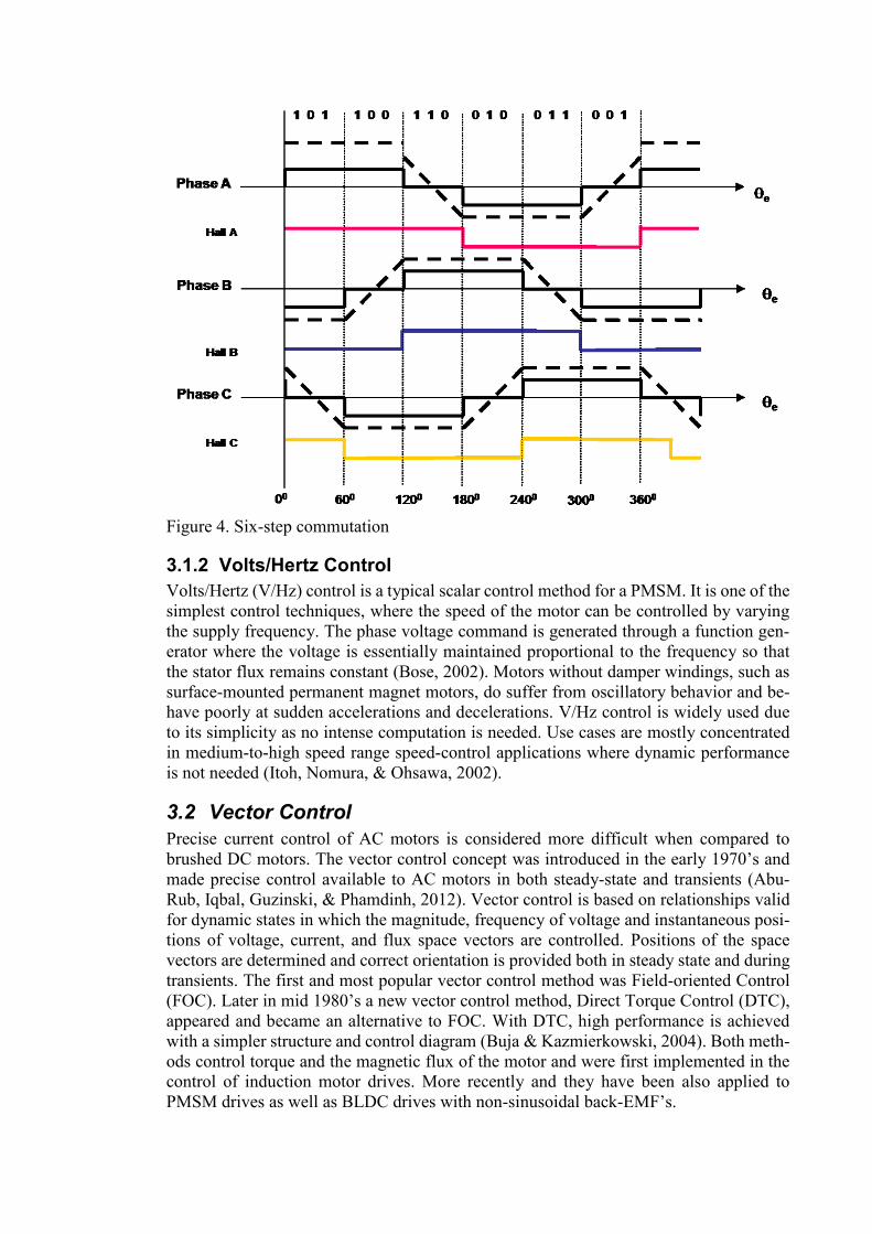
Figure 4. Six-step commutation

3.1.2 Volts/Hertz Control Volts/Hertz (V/Hz) control is a typical scalar control method for a PMSM. It is one of the simplest control techniques, where the speed of the motor can be controlled by varying the supply frequency. The phase voltage command is generated through a function gen-erator where the voltage is essentially maintained proportional to the frequency so that the stator flux remains constant (Bose, 2002). Motors without damper windings, such as surface-mounted permanent magnet motors, do suffer from oscillatory behavior and be-have poorly at sudden accelerations and decelerations. V/Hz control is widely used due to its simplicity as no intense computation is needed. Use cases are mostly concentrated in medium-to-high speed range speed-control applications where dynamic performance is not needed (Itoh, Nomura, & Ohsawa, 2002).

3.2 Vector Control Precise current control of AC motors is considered more difficult when compared to brushed DC motors. The vector control concept was introduced in the early 1970’s and made precise control available to AC motors in both steady-state and transients (Abu-Rub, Iqbal, Guzinski, & Phamdinh, 2012). Vector control is based on relationships valid for dynamic states in which the magnitude, frequency of voltage and instantaneous posi-tions of voltage, current, and flux space vectors are controlled. Positions of the space vectors are determined and correct orientation is provided both in steady state and during transients. The first and most popular vector control method was Field-oriented Control (FOC). Later in mid 1980’s a new vector control method, Direct Torque Control (DTC), appeared and became an alternative to FOC. With DTC, high performance is achieved with a simpler structure and control diagram (Buja & Kazmierkowski, 2004). Both meth-ods control torque and the magnetic flux of the motor and were first implemented in the control of induction motor drives. More recently and they have been also applied to PMSM drives as well as BLDC drives with non-sinusoidal back-EMF’s.

12

3.2.1 Field-oriented Control Field-oriented control (FOC) makes it possible to control the current of a PMSM like in a brushed DC motor and achieve an equivalent torque control performance. This is made possible by transforming the three-phase stator currents into a two-axis system in a rotat-ing reference frame synchronized with the rotor flux. Resulting currents act like DC cur-rents and can be controlled with simple PI controllers. For ideal behavior, the following transformation models can be used only for motors with sinusoidal back-EMFs but recent findings have presented models that extend the transformations for a BLDC motor.

Figure 5. FOC Block Diagram

The control process starts by measuring the currents in two of the stator windings. These are transformed with a Clarke (or alpha-beta) transformation into a two-axis, alpha-beta, reference frame. It can be thought of as the projection of the three currents onto two sta-tionary axes, the alpha axis and the beta axis as shown in figure 6. The resulting two-phase current waveforms have an equivalent amplitude as the original current waveforms in three-phase. Next, a Park (or dq, direct-quadrature) transformation is performed to con-vert the two-axis system from a static reference to a rotating reference frame synchronized with the rotor flux. This results into d and q currents. The d axis current is aligned with the rotor flux while the q axis is orthogonal to the rotor flux. Therefore, the q axis current represents the torque production of the motor. Both d and q axis currents are controlled with PI controllers that read current error signals and produce voltage to control the mo-tor. Figure 5 shows a simplified illustration of the process. As torque is proportional to current, the target torque can be fed directly to the current control loop.

Figure 6. FOC transformations illustrated Before feeding voltage to the motor, the voltages have to be converted back to a stationary reference frame and to a three-axis system. This is achieved by an inverse Park transfor-mation and an inverse Clarke transformation, respectively. The resulting three voltages are now applied to the stator windings. The stator currents in the dq frame are given as

[𝑖𝑑𝑠𝑖𝑞𝑠

] =23

[𝑠𝑖𝑛𝜃𝑟 sin (𝜃𝑟 −

2𝜋3

) sin (𝜃𝑟 +2𝜋3

)

𝑐𝑜𝑠𝜃𝑟 cos (𝜃𝑟 −2𝜋3

) cos (𝜃𝑟 +2𝜋3

)] [

𝑖𝑎𝑠𝑖𝑏𝑠𝑖𝑐𝑠

] (13)

where θr is the rotor angle and ias, ibs and ics are balanced three phase stator currents. The same representation applies also for stator voltages in the dq axis. δ is the angle between the stator current is and the rotor field. This is also called as the torque angle. Thus, stator currents can be also written as

𝑖𝑎𝑠 = 𝑖𝑠 sin(𝜃r + δ) (14)

𝑖𝑏𝑠 = 𝑖𝑠 sin (𝜃r + δ −2π3

) (15)

𝑖𝑐𝑠 = 𝑖𝑠 sin (𝜃r + δ +2π3

) (16)

The stator current is related to the stator current d and q components by

[𝑖𝑑𝑠𝑖𝑞𝑠

] = 𝑖𝑠 [𝑐𝑜𝑠𝛿𝑠𝑖𝑛𝛿] (17)

In a reference frame synchronized with the rotor, the stator dq currents are constant. This is because δ is constant for the determined torque and the rotor runs at a synchronous speed. Therefore, the electromagnetic torque can be represented as follows

𝑇𝑒 =32

𝑝 [12

(𝐿𝑑 − 𝐿𝑞)𝑖𝑠2𝑠𝑖𝑛2𝛿 + 𝜓𝑓𝑖𝑠𝑠𝑖𝑛𝛿] (18)

where Ld and Lq are winding inductances of d and q axis. Lm is the mutual induction between the rotor magnet and the stator windings. Ψf represents the permanent magnet

14

flux which is always along the d axis. As seen, torque mostly depends on issin δ. There-fore, q current is equivalent to the armature current of a brushed dc motor. At δ = π/2, torque is

𝑇𝑒 =32

𝑝𝜓𝑓𝑖𝑠 (19)

It can be seen that, if the torque angle is 90 degrees and the flux is constant, the motor torque can be controlled with the magnitude of the stator current.

3.2.2 Direct Torque Control Direct torque control (DTC) is a technique that enables direct control of flux and torque. The flux set point and the torque set point are used as control references and to establish a closed loop flux and torque control, DTC requires estimation of the motor torque and stator flux. The existing errors in flux and torque can be used directly to drive the inverter without a separate current control loop or coordinate transformation. Therefore no rotor position sensor is needed. In conventional DTC models, flux and torque are controlled with a hysteresis type of controller that determines which of the possible inverter states should be applied to keep the error in the flux and torque within the prescribed hysteresis bands. A more detailed description of a hysteresis controller is presented in section 3.4.3. In DTC, it is essential to have an accurate machine model as the stator flux and motor torque estimation is based on the model and motor input stator voltage and current meas-urements. The stator flux is estimated in a stationary reference frame where the stator flux linkage can be obtained by integrating the stator EMF. Estimations are made based on the following equations which are expressed in the dq reference frame.

𝑣𝑑𝑠 = 𝑅𝑠𝑖𝑑𝑠 +𝑑𝜓𝑑

𝑑𝑡− 𝜔𝜓𝑞 (20)

𝑣𝑞𝑠 = 𝑅𝑠𝑖𝑞𝑠 +𝑑𝜓𝑞

𝑑𝑡− 𝜔𝜓𝑑 (21)

𝜓𝑑 = 𝐿𝑑𝑖𝑑 + 𝜓𝑓 (22)

𝜓𝑞 = 𝐿𝑞𝑖𝑞 (23)

As the rotor of the PMSM is a permanent magnet, the electromagnetic torque equation is as follows

𝑇𝑒 =32

𝑝(𝜓𝑓𝑖𝑞 − (𝐿𝑑 − 𝐿𝑞)𝑖𝑞𝑖𝑑) (24)

𝑑𝜔𝑑𝑡

=1𝐽

(𝑇𝑒 − 𝑇𝐿)

(25)

where ω is the motor angular speed, J moment of inertia and TL motor load. Thus, the following relationship can be derived

𝑇𝑒 =32

𝑝𝜓𝑠−𝑟𝑒𝑓

𝐿𝑑𝐿𝑞(𝜓𝑓𝐿𝑞𝑠𝑖𝑛𝛿 +

12

𝜓𝑠−𝑟𝑒𝑓(𝐿𝑑−𝐿𝑞)𝑠𝑖𝑛2𝛿) (26)

From equation 26 it can be seen that for constant stator flux amplitude and permanent magnet flux, the electromagnetic torque can be controlled by the torque angle δ. This is the angle between the rotor flux linkage and stator, when the stator resistance is neglected. The torque angel can be changed by changing the stator flux vector position in respect to the permanent magnet flux vector using the actual voltage vector supplied by the inverter. In steady state δ is constant and corresponds to a load torque, whereas stator and rotor flux rotate at synchronous speed. In transient operation, δ varies and the stator and rotor flux rotate at different speeds. (T. Zhang, Liu, & Zhang, 2010)

A conventional DTC scheme uses two hysteresis comparators and a switching table which enables quick dynamic response but might cause undesired torque ripple, acoustic noises and has a variable switching frequency. To overcome the issues, the hys-teresis controller can be replaced with a voltage modulator. Space vector modulation (SVM) is a modulation technique commonly used in DTC to create continuous voltage vectors, that can adjust torque and flux precisely and moderately (Y. Zhang & Zhu, 2011). Using SVM requires also a lower sampling frequency. However in the SVM-based DTC models, a rotary coordinate transformation is often needed, which makes it more compu-tationally intensive than the conventional DTC (Zhong, Rahman, Hu, Lim, & Rahman, 1999). The SVM model is presented in section 3.4.2.

3.2.3 Feasibility for Position Control From a torque control perspective, position control is more challenging than speed con-trol. Fast accelerations and decelerations require a constant change in torque while tran-sitions might be short and maximum speeds remain low. In general, scalar control meth-ods do not provide as fast and stable torque control as would be needed for fast position-ing. (Itoh et al., 2002) Besides, all torque control methods require high resolution rotor position or speed data to produce smooth torque at low frequencies which excludes most sensorless estimation methods.

Vector control methods provide more dynamic torque control which is seen suitable for positioning applications. Performance-wise, a conventional DTC scheme is consid-ered as the fastest method while FOC and SVM-DTC schemes induce less torque rip-ple(Garcia, Zigmund, Terlizzi, Pavlanin, & Salvatore, 2011). FOC is computationally more intense which was seen as a problem still in the early 2000’s. but not at the same extent anymore as the availability of cost-efficient powerful MCUs has decreased. As a theory FOC is already rather mature and widely used in industrial applications. Software libraries and dedicated IC’s are commercially available. At the same time, apart from the electric drive manufacturer ABB’s products, DTC is still quite rarely used in the industry and few software or hardware is commercially available.

3.3 Harmonic Factors In order to create a high-performance position control, it is essential to achieve torque smoothness. Current control schemes aim to create a torque close the given reference. Due to harmonic factors, this is not always easily achievable. Resonance and ripple cause also audible noise. Causes can be classified into three main groups: motor, inverter and load induced factors.

The most remarkable factors in the motor causing torque ripple are cogging torque, mutual torque and reluctance torque. Cogging torque is induced by stator slots that interact with the rotor magnetic field. Variation in phase inductance, which is relative to position, produces reluctance torque while mutual torque is caused by mutual coupling between the rotor magnetic field and stator winding current (Wang, Kamper, Westhuizen, & Gieras, 2005). Other factors, such as flux linkage harmonics caused by magnetic satu-ration and iron stator slots can be neglected for a coreless stator motor. In practice, a large

16

air gap between the stator and rotor minimizes harmonics produced by the stator back-EMF space distribution. Due to the fast change of phases and low inductance stator wind-ings caused by the coreless design, cogging torque and reluctance torque have only a minor effect which makes it possible to concentrate in minimizing mutual torque (Fang et al., 2012). Besides harmonics caused directly by the motor design, a major part of torque ripple might be caused by the inverter not capable to produce ideal voltage waves. In general, torque ripple remains modest by matching the waveforms of the phase current and phase back-EMF. Most current control schemes presume a sinusoidal back-EMF while in practice it is often not the case. For surface mounted PMSMs, the gap between two adjacent permanent magnets always exists no matter how close they are placed. Thus the back EMF will always contain high-order harmonics (Xinda & Bangcheng, 2016). Also, modulation of a three-phase inverter induces remarkable torque ripple caused by the small inductance of a small brushless DC motor and is discussed more in section 3.4. Low inductance is a consequence of a coreless stator structure which is typical in small size and light weight motors. This can be compensated by increasing switching frequency but limitations are set by the controller performance (Fang et al., 2012). Some of the harmonics are purely caused by the inverter hardware. In an inverter, non-sinusoidal volt-ages results in a non-sinusoidal current. These are caused by non-linear power electronic components, inaccurate current measurements, delays in sampling and filters and dead-time between switching. Torregrossa et al. (2012) and Laurila, (2004) present analytical models of the harmonic orders resulted from each component. Besides harmonics, most current control schemes require precise current measurement to perform as expected. For small inductance motors it is challenging as current drops quickly during measurement intervals. Load induced ripple is caused by bearings, load and motor shaft couplings, gearings and the load itself. Mechanical defects such as problems in bearings and cou-plings might also cause static eccentricity which means that the center of the rotor is dis-placed to a fixed eccentric position. This is critical because it results in an asymmetrical distribution of the flux density at the air gap between the stator and rotor and thereby causes additional harmonics (Coenen, Herranz Gracia, & Hameyer, 2011).

3.4 Inverter Techniques After the current control loop, a dc-to-ac power conversion is performed in an inverter. Inverters can be broadly classified in two groups: voltage source inverters (VSI) and cur-rent source inverters (CSI). In voltage source inverters DC voltage is kept constant while in current source inverters input current is kept constant. As discussed in section 3.2, controlling current enables high precision torque control and therefore is essential in ac-curate positioning. Therefore, all inverters presented are current controlled or in other words voltage source inverters. Current source or multi-level inverters are rarely used in smaller brushless DC drives and therefore not discussed in the scope of this thesis. The following sub-sections introduce the most typical pulsing methods of a conventional two-level three-phase VSI.

A typical filterless, low voltage and current VSI consists of 3 MOSFET bridges. This means 6 power MOSFET switches and 6 diodes as seen in figure 6. The three generated phases are A, B and C (U, V, W in figure 6).

Figure 6. Circuit diagram of a three-phase VSI with AC motor

3.4.1 Pulse Width Modulation Pulse width modulation (PWM) is a method for creating an analog signal with a digital source. PWM controls the inverter switches in such a way that the output voltage consists of a row of pulses. Each pulse is separated with “notches” that represent zero state. Duty cycle of a switch represents the time the signal is in high state relative to the time of it takes to complete one cycle.

𝑑 = 𝑡𝑜𝑛

𝑡𝑜𝑛 + 𝑡𝑜𝑓𝑓(27)

Where ton is the time when the switch is on while toff denotes off-time. The average value, Vdc, of the output voltage is proportional to the duty cycle, d12, and the fixed value of the high voltage level, vi.

𝑣𝑑𝑐 = 𝑑12𝑣𝑖 (28) As seen, the duty ratio can be adjusted from 0 to 1 which enables adjusting the output voltage Vdc from 0 to Vi. Switching frequency fsw is defined as

𝑓𝑠𝑤 =1

𝑡𝑜𝑛 + 𝑡𝑜𝑓𝑓 (29)

Switching frequency describes how fast the PWM completes the cycle and therefore how fast it is switched between high and low states. It does not affect the output voltage Vdc but rather to its quality. By keeping the time between consecutive state changes short, significant current changes between consecutive states can be prevented. The output volt-age harmonics are around the integer multiples of the switching frequency (Bose, 2002). As an inductive component, the PMSM stators oppose current changes which smoothens the output waveform close to an ideal dc quality. However, this does not fully apply for small motors that have a low inductance. In an electrical circuit, the interaction between voltage v, inductance L and current i can be described as follows:

𝑣 = 𝐿𝑑𝑖𝑑𝑡

(30)

18

As can be seen, current change is related to the voltage and inductance. A smaller induct-ance causes current to rise faster which grows the PWM induced current and torque rip-ple. This is often compensated with a higher switching frequency. The effect of an in-creased switching frequency can be seen in figure 7 and 8.

Figure 7. Current as a function of time, 50% duty cycle, fsw = 33 Hz

Figure 8. Current as a function of time, 50% duty cycle, fsw = 1000Hz It is clear that a higher switching frequency improves the output current quality. However in practical devices, switching frequency is restricted due to the limitations of the control system performance, operating frequency of the switches and switching losses of practical switches (Trzynadlowski, 2016). Therefore the switching frequency selection is always a tradeoff between quality and efficiency.

3.4.2 Space-Vector Modulation Various PWM techniques have been presented to determine the timing of opening and closing switches. Differences are typically related in output current quality and output voltage level maximums. Three-phase voltage-source inverter applications like PMSM control use mainly space-vector modulation PWM (SVM) which, compared to other ap-proaches, is considered as an advanced but computationally more intensive technique. It enables a high output quality, a low harmonic distortion and a flexible control over output voltage and frequency (Bose, 2003).

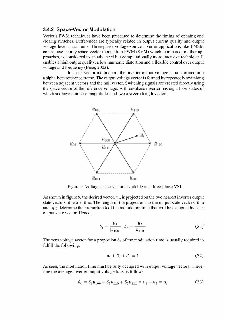
In space-vector modulation, the inverter output voltage is transformed into a alpha-beta reference frame. The output voltage vector is formed by repeatedly switching between adjacent vectors and the null vector. Switching signals are created directly using the space vector of the reference voltage. A three-phase inverter has eight base states of which six have non-zero magnitudes and two are zero length vectors.

Figure 9. Voltage space-vectors available in a three-phase VSI

As shown in figure 9, the desired vector, us, is projected on the two nearest inverter output state vectors, û100 and û110. The length of the projections to the output state vectors, û100 and û110 determine the proportion δ of the modulation time that will be occupied by each output state vector. Hence,

𝛿1 =|𝑢1|

|�̅�100| , 𝛿2 =|𝑢2|

|�̅�110| (31)

The zero voltage vector for a proportion δ3 of the modulation time is usually required to fulfill the following:

𝛿1 + 𝛿2 + 𝛿3 = 1 (32) As seen, the modulation time must be fully occupied with output voltage vectors. There-fore the average inverter output voltage ûo is as follows

�̂�𝑜 = 𝛿1𝑢100 + 𝛿2𝑢110 + 𝛿3𝑢111 = 𝑢1 + 𝑢2 = 𝑢𝑠 (33)

20

3.4.3 Hysteresis Controller A hysteresis controller is a feedback controller that switches rapidly between two states. It is a type of a bang-bang non-linear controller that provides an extremely fast dynamic response due to the absence of a modulator. It is argued that no linear controller can achieve the same performance (Buso & Mattavelli, 2006). As seen in figure 10, the state of the inverter high and low side switches is determined directly by comparing the instan-taneous inverter current with the given reference. A hysteresis controller is typically im-plemented analogically due to its high sampling frequency needed for digital, discrete implementation which is also called as sampled hysteresis (Buja & Kazmierkowski, 2004).

Figure 10. Hysteresis current control

In practice, a comparator tracks the instantaneous current error, and drives directly the converter switches. As the dc link voltage is always higher than the output voltage peak value, the current derivative is positive always when the high-state switch is closed and negative when the low-state switch is closed. Therefore, the controller will maintain the inverter output current close to its reference. The hysteresis bandwidth determines the limits for negative and positive errors. The current error can be minimized to near zero by setting a zero hysteresis bandwidth and increasing switching frequency but as in the case of a PWM, switching frequency selection is always a compromise of quality and an increased dead-time and switching losses. Despite of the fast response and high tracking capabilities, hysteresis con-trollers are not the most common choice for PMSM drives. The main drawback is its variable switching frequency which makes it hard to filter high frequency voltage and current components. Increased torque ripple and acoustic noise have also been seen as a negative consequences (Y. Zhang & Zhu, 2011).

3.5 Position Sensing Accurate rotor position feedback is an essential part of advanced current control methods such as FOC while the same information is also used for accurate position and speed control. Angle feedback is typically obtained with position sensors such as rotary encod-ers or hall effect sensors. Rotary encoders can be generally divided into absolute and incremental encoders.

3.5.1 Incremental Encoders Incremental encoders provide a simple quadrature output of A and B pulses which are decoded in an external unit. Typically, the encoder supplies square-wave signals in two channels that are offset from each other by 90 degrees. These channels indicate both po-sition and direction of rotation. Each rotation increment creates an output pulse. As seen

in figure 11, direction can be determined by comparing A and B channel outputs. For example, if A leads B the rotor is rotating in a clockwise direction and if B leads A, then the rotor is rotating in a counter-clockwise direction. Pulses are counted from the startup point and each mechanical rotation ends to a reference point which is often implemented with an index pulse. Each time the encoder is turned on it begins to count from zero, regardless of its position earlier. The amount of pulses per revolution (PPR) are also measures of resolution for an incremental encoder. An incremental encoder does not pro-vide position information on startup but this can be obtained by referencing the shaft in a zero point or recording the angle somehow else. These type of encoders are generally simple by construction and therefore also cost-efficient. Incremental encoders can also be fitted in a small space and are light weight.

Figure 11. Quadrature pulses Typical designs of incremental rotary encoders are magnetic and optical. A magnetic en-coder consists of a rotor and a sensor. The rotor rotates with the motor output shaft and contains evenly spaced south and north poles around its ring. Shifts in position are sensed by detecting poles changing from N to S or S to N. Sensing is implemented either with a Hall Effect sensor or a Magneto resistive sensor. A Hall Effect sensor works by detecting changes in voltage responding to a magnetic field while a Magneto resistive sensor tracks changes in resistance caused by a magnetic field (Kuttan, 2007). Optical rotary encoders on the other hand consist of a light source, a sensor, a movable disc and a fixed mask. The disc is attached to the rotating shaft while the disc has a series of tracks on its periph-eral. The mask has an equivalent track for every track on the, and small holes are made along the tracks in the mask. As the disk rotates, holes in the mask are either covered or open, showing the movement and position of the optical encoder (Ireland, n.d.). Like any other optical systems, optical encoders are considered accurate but also sensitive to dis-turbances and environmental contamination. Magnetic encoders are, on the other hand, extremely robust and tolerate levels of dust, shock and vibration. The magnet is however intolerant for displacement and might cause non-linearities in the output angle data.

22

Figure 12. Left: incremental encoder, right: absolute encoder

3.5.2 Absolute Encoders Absolute encoders provide unique position values and maintain position information when power is turned off. As seen in figure 12, this type of encoder has a encoder disc that has marks or slots on a shaft and a stationary pickup. Each shaft position sequence provides a unique code. As each position sequence is unique, the encoder records also movement that has happened while power is off. The ability to maintain position infor-mation is often a benefit when using a PMSM as the rotor position has to be known for commutation. Typical communication interfaces are serial interfaces such as SPI or SSI but PWM interfaces are also used. These benefits often come with the drawback of a more complex design and higher unit cost. Some limitations for usage is set by the more com-plex communication interfaces. Many commercial motor controllers do not support com-munication with an absolute encoders by default and extra effort has to be done for im-plementation. Similar to the incremental encoders, absolute encoders are typically either magnetic or optical by design and can be described with the same features as in section 3.6.1.

3.5.3 Hall Effect Sensors Hall effect sensors are transducers that vary their output voltage in response to a magnetic field. Besides usage in magnetic rotary encoders, they can be installed inside the motor to detect the bypassing rotor permanent magnets (figure 13).

Figure 13. Placement of Hall Effect Sensors

Hall effect sensors are either digital or analog (linear). Digital sensors have a Schmitt-trigger with built in hysteresis connected to the op-amp. The built-in hysteresis decreases oscillation of the output signal. When the magnetic flux passing through the sensor ex-ceeds a pre-determined value, the output signal switches between an “OFF” condition to an “ON”. Analog sensors differ in a way that the output is a continuous voltage that in-creases with a strong magnetic field and decreases with a weak magnetic field.

Therefore, the working principle of a digital hall effect sensor in a motor is simple: when the rotor passes a hall-effect sensor, a high or a low signal is created to express which rotor pole (N or S) has passed. Therefore, switching signals of the three hall effect sensors (from high to low or from low to high) provide rotor position data with a 60 degree resolution. An analog hall effect sensor on the other hand increases the output voltage when approaching the rotor, provides the peak voltage during bypass and de-creases while growing the distance. Outputs are shown in figure 14 and 15.

Figure 14. Analog Hall Effect Sensor output

24

Figure 15. Digital Hall Effect Sensor output Hall effect sensors are considered as a cost-efficient way to determine rotor position feed-back. Sensors are cheap and can be installed directly to the motor. No extra space or installations is therefore needed which is beneficial in small size applications. Limitations are set by resolution: a typical setup with three digital hall effect sensors is able to produce position information every 60 degrees which is not enough for most position control ap-plications. Combined with an incremental encoder, digital hall effect sensors can be used for motor startup. An incremental encoder does not remember its position during shut down while a digital hall effect sensor provides a value immediately after startup. After a short movement, feedback input can be switched to back to the primary incremental encoder. Analog hall effect sensors on the other hand provide more resolution. In digital control, the resolution of the rotor angle estimate (pulses per revolution, PPR) is determined from the maximum peak-to-peak voltage (vpp) of the hall effect sensors and ADC resolution (vADC) as follows

𝑣𝐴𝐷𝐶 =𝑣𝐹𝑆𝑉

2𝑀 (34)

𝑃𝑃𝑅 =𝑣𝑝𝑝

𝑣𝐴𝐷𝐶(35)

where M is the ADC resolution in bits and vFSV the full scale voltage of the converter. It is feasible to achieve resolutions over 1000 PPR with optimal ADC and hall effect sensor peak-to-peak voltage values. Despite the high theoretical resolution, most implementa-tions suffer from poor accuracy due to uncertainties such as the influence of magnetic and mechanical tolerances, temperature variations, and the armature reaction field (Xinda & Bangcheng, 2016). Consequently, the output signal will be distorted to nonstandard sine wave. Most position estimation methods are based on the assumption that each hall effect sensor is exactly aligned with stator magnetic axes and stator poles are not displaced. Therefore, various approaches have been suggested to compensate the misalignment ef-fect of hall effect sensors. Beccue et al. (2007) present a routine for compensating the offset in hall effect sensor placement. The resultant actual state transition values are stored in a lookup table. The drawback of this algorithm is that it is based on the average speed of the motor and loses performance in variable speed operation. Yoo et al. (2009) suggests improved observers for position and speed estimation that show promising results in var-iable speed control tests with a washing machine. For signal filtering, it is presented that the output signal harmonics could be filtered with a notch filter (Karimi-Ghartemani, Khajehoddin, Jain, Bakhshai, & Mojiri, 2012).

3.6 Sensorless Control Generally, the brushless DC drive requires continuous rotor position feedback to form proper current waveforms in the inverter. A shaft position sensor provides accurate infor-mation but has its drawbacks including the increased cost, complexity and size. To bypass the downsides, methods to estimate the rotor position without a sensor have been pre-sented.

A typical approach for sensorless control is to integrate the output voltage of a PWM inverter to determine the stator flux and determine the rotor position from the current angle. Stator and rotor flux vectors rotate synchronously in steady state. The angle difference between these two space vectors is equivalent to the load torque angle. The rotor flux angle, which indicates rotor position, can be calculated if the stator flux vector is known. For a PMSM, mathematic equations are symmetric in αβ coordinates. This method works in open loop but is vulnerable to parameter uncertainty (Yongdong & Hao, 2008). Therefore, a low pass filter is used to replace a pure integrator, which on the other hand causes a delay and thus an error in the rotor position estimation at low speeds. Pre-cisely, the EMF space vector, e, can be determined by measuring the stator line-to-line voltages, v, and phase currents, i, as follows (Aḥmad, 2010)

𝑒 = 𝑣 − 𝑅𝑠𝑖 (36) The resulting value is integrated as follows

𝜓 = ∫ 𝑒 𝑑𝑡 (37)

which results as the flux linkage space vector. The space angle of flux is obtained from its real and imaginary components as

𝜃𝜓 = tan−1 (𝜓𝐼

𝜓𝑅) (38)

The model has two shortcomings that degrade performance as speed reduces. Firstly, in-tegration creates a problem and secondly it is sensitive to stator resistance mismatch (Yongdong & Hao, 2008). Therefore, it is not suitable for high accuracy applications. Other advanced methods include the Extended Kalman Filter (EKF) and High Frequency Injection (HFI) of which the first is a stochastic state observation based on least–square variance estimation extended to a non-linear system. It is considered as more accurate than the back-EMF integration method but computationally intensive which limits its usage in industrial applications. The HF injection method is based on the motors magnetic saliency property and thus considered as insensitive for parameter inac-curacy. In practice, high frequency signals are injected to the PMSM. As the injected voltage or current signals have a varying frequency from the fundamental, the response signals can be used to determine spatial information. This method provides good results already on low speeds but requires a salient rotor structure which is barely used in small motors. In general, sensorless rotor position estimation methods have been success-fully implemented in speed controllers optimized for higher frequencies. All methods for non-salient motors lack the capability to estimate accurately positions at low-frequencies which is essential in high accuracy position control.

26

3.7 Control Architectures for Position Control A key part of this thesis is to find ways to position the determined load in a limited time frame. This includes reaching the specified settling time target as well as settling accu-racy. The environment is closed and active forces are known which decreases the need for robustness. However, the system has to be able to handle uncertainties in electrical and mechanical components. This could mean parameter variations for example in torque constant of the motor and vibration mode frequencies due to temperature fluctuation and/or aged degradations, system delay components, and unpredicted disturbances from environments (Iwasaki, Seki, & Maeda, 2012). To achieve the required response and pre-cision, several closed-loop position control methods and different tuning approaches have been proposed ranging from tuning a simple proportional integral (PI) controller to the use of complex nonlinear controllers.

A classical position control system is implemented with PI controllers and contains at least two cascade control loops, one for torque regulation and other for posi-tion control. A speed control loop typically added between the torque loop and the posi-tion loop, leading to a three-loop position control system. The intermediate speed control loop adds robustness against parameter variations due to temperature sensitivity of the magnets and helps to optimize the velocity profiles (Palacios, 2017). The classical PI controller is considered as simple and good enough for many applications which have a close-to linear behavior and can be modeled by a first-order differential equation. Lacking dynamic response can be improved by adding a feed-forward compensator to the system. A feedback controller has always a delay and reacts passively to all disturbances. If the system behavior is known, part of the control input can be pre-determined and thus delays can be decreased. This requires that the disturbances are measured and accounted for be-fore they have time to affect the system. Therefore, the precise modeling of the system is essential. This should include load side disturbances as well as non-idealities in the motor structure. A more precise system model enables higher compensation in the feedforward manner as well as a more aggressive design in the feedback controller (Iwasaki et al., 2012).

Typically, the system cannot be modelled perfectly as mechanical systems and non-ideal motors produce resonances at certain frequencies. This creates challenges to the conventional position control scheme. Therefore, frequency-dependent filtering is used to filter undesired regions of the operational frequency spectrum. This might be use-ful in systems that resonate at a certain frequency or speed, or to reduce high-frequency noise. In practice, these can be used to filter either feedback data or the target values. For example, a filter for the torque target value can be used as a low-pass filter for bandwidth limitation and noise suppression. Moreover, it can be designed to suppress a resonance or anti-resonance (Lewin, 2006). A typical implementation of a filter limiting bandwidth is known as a biquad filter. Biquad filters are common in digital control systems since they are considered flexible and easy to implement. A biquad filter can be designed to operate as a notch, bandpass, band reject, or high or low-pass filter. A biquad filter can be repre-sented as:

𝑌𝑛 = 𝐾(𝐵0𝑋𝑛 + 𝐵1𝑋𝑛−1 + 𝐵2𝑋𝑛−2 + 𝐴1𝑌𝑛−1 + 𝐴2𝑌𝑛−1) (39) where Yn is the filter's output at time n, Xn is the filter's input at time n, K is a positive scalar gain and B0, B1, B2, A0, A1 are programmable biquad coefficients. B0, B1, B2 de-termine the zeros while A1, A2 determine the position of poles.

3.8 Digital Control Most controllers today are based on digital controllers implemented on microprocessors and digital signal processors (DSP). Advantages of digital control are related to the ability to incorporate complex control algorithms and filtering. Functions can be reprogrammed and corrected with low effort. The most remarkable disadvantage is related to the fact that digital controllers do not process analog signals directly. Instead, the signals are sampled. Between successive samples no information is obtained on the intermediate value of the analog signal. This can be handled by keeping the time intervals between samplings clearly shorter than the time constant of the controlled process. Due to this, a sudden disturbance is detected in the controller after an average time of half a sampling period. The sampled version is therefore delayed compared with the actual signal, and the delay is approximately half the sampling period (Tan & Putra, 2011). The delay can be mini-mized by increasing the controller sampling frequency. Due to the decreased cost of com-putation power, high sampling frequencies have been made possible even on low-cost microcontrollers. However, still some of the most high speed applications are imple-mented analogically. Analog controllers operate in real time and do not require sampling. Therefore, some digital motor controllers include analog components to execute tasks like filtering or multiplying.

3.9 Power Transmission In mechatronic applications the motor and transmission must be chosen in consideration of each other. Characteristics of both components affect the selection of a suitable power transmission. In particular, the speed range of the motor related to the torque characteris-tics, are generally decisive because of the constraints that they impose on the choice. In the scope of this thesis, possible implementations are a direct-drive and a geared trans-mission. Gearboxes are used to convert the lower torque output of the motor to achieve a higher torque at a usable speed. This also decreases the demand for high accuracy motor control. Ripple effects on the motor are smaller on the load-side due to the reduction made by the gears. Minor overshoot and settling issues on the motor output shaft might be neg-ligible on the load-side. At high speeds, torque ripple is mostly filtered out by the rotor inertia (Mandel & Weiss, 2009). However, at lower speeds torque ripple produces notice-able effects that create undesirable speed variations, and cause inaccuracy in motion con-trol. Similarly reduction allows the system to use the lower torque motors that might save weight and costs.

A major drawback in gearing is the backlash caused by the gear mechanic structure making it as a two-mass system. Backlash is the slack in the system, also referred to as the play in the gears meaning that the load-side position is always misaligned to the motor output shaft. Eliminating backlash is difficult with multiple stage gearboxes. Gears have to be manufactured with very tight fit, or tolerance, which can be costly. In addition, tight tolerances lead to high friction, or a mechanism is needed to keep the gears tightly engaged over their range of torque. Flexible gear systems, like a strain wave gear, offer another method to help eliminate backlash, since the gearbox has some flexible compo-nents that take up the slack. Unfortunately, this can lead to potential fragility and makes back driving, operating the device in reverse, very difficult. Therefore, backlash compen-sation is often done in the controller software by taking in account the exact backlash of the particular gearbox. This takes time and requires recalibration after mechanical wear which is inevitable in all gears. Due to the restrictions related to the elimination or com-pensation methods, a second position encoder is often used to track the position of the load. This method is often needed in high performance applications requiring exact posi-tion control. An advanced torque control method, like FOC, requires accurate position information meaning that the position sensor is attached directly to the motor output shaft

28

(Nordin & Gutman, 2002). Therefore, a load-side position sensor cannot be used for con-trolling torque. Load-side position information provided by the second encoder is used as a feedback for the position controller enabling the controller to position the load as re-quired regardless of the backlash. This method is effective but increases the system weight, cost and complexity.

The most basic type of gear is the spur gear, where the teeth within the gear will come into full contact for each engagement, causing noise, and leading to wear and often the need for lubrication (figure 15). A more advanced gear type fixing some of the disadvantages is a planetary gear (figure 16). It consists of several planet gears, a sun gear and a ring gear or annulus. In addition, it includes a movable arm or a carrier holding the planet gears. The movable arm and the planet gears rotate around the sun gear. The outer gear or annulus rotates along with the planet gears. Usually, axes of the gears are parallel to each other and are concentric. These lead to a more compact size, higher efficiency, and lower noise level than for spur gears. Disadvantages of a planetary gear system in-clude design complexity, high bearing load and inaccessibility.

Figure 15. Spur gears

Figure 16. Planetary gear

In a direct-drive actuator the load is driven directly from the motor output shaft thus no gearbox is used. It requires the motor to be able to produce enough native torque at a usable speed which in the scope of this thesis means not thousands of RPMs, but hundreds of RPMs. Direct-drive has no backlash because there are no gears; the torsional stiffness provides very high precision. Direct-drive has also no restrictions for back-driving. Pre-cision however requires high controller performance. All ripple effects and settling issues are directly seen in the load which requires careful tuning of the control system. Another major disadvantage is related to the higher torque required from the motor, which in-creases the motor weight and cost. However, the system complexity is lower and requires less supporting components.

4 System Model The application can be described as a rotating electrical-drive system. The mechanical dynamics can be derived from Newton’s law of rotating bodies using the motor inertia JM and load inertia JL. The free end of the axle is attached to a bearing. The system is modeled as a single-mass system due to the overdamped nature of the system which reduces higher order vibrations.

Figure 5. System model

TL Te ω

30

4.1 Single-Mass Model The model of a system represented in figure 17 is the following:

𝐽𝑑𝜔𝑑𝑡

= 𝑇𝑒 − 𝑇𝐿 where J is the total moment of inertia of the system. Te is the electromagnetic torque produced by the motor and ω is the angular speed of the motor. Load torque is represented as TL which is produced by the bearing friction and the internal inertia and friction of the motor. The required angular speed can be derived from the maximum angle that the plate will turn:

𝜔 = 𝑑𝜃𝑚𝑎𝑥

𝑑𝑡

The total moment of inertia for a rectangular plate where its rotational axis goes through the center in the plane of the plate is as follows:

𝐽𝑐𝑚 =1

12𝑚𝐿2

Figure 18. Total moment of inertia for a rectangular plate

where m is the mass and L is the height of the plate, respectively. However, the above mentioned moment of inertia does not apply as the desired axis of rotation is not in the center of gravity of the plate. Therefore, based on the Steiner theorem the new moment of inertia is as follows:

𝐽 = 𝐽𝑐𝑚 + 𝑚𝑑2 = 𝑚(1

12𝐿2 + 𝑑2)

where d is the perpendicular distance between the axes.

Figure 19. Plate measures

4.2 Numerical Models The numerical values of the system are defined based on values given by the manufac-turer. The plate material is toughened glass and the frames are made of plastic. Mass of the system is 5.9 grams including the plastic frames but excluding the bearing shown in figure 19. The center line of mass in the plane of the plate is 3.5 mm below the desired axis of rotation. Maximum rotation for the plate is 10°, which shall be executed in 10 ms. The torque produced by the motor rotor inertia is assumed as cJ = 0.1 mNm and the motor friction torque as c = 0.02 mNm. The torque caused by air drag can be estimated as cD =0.3 mNm with a drag coefficient of 2 and maximum speed of 3 m/s. Bearing friction is neglected. Therefore, the maximum required motor torque can be defined from the following:

𝑇𝑒 = 𝐽𝑑𝜔𝑑𝑡

+ 𝑇𝐿 (40)

𝑇𝑒 = (𝑚 (1

12𝐿2 + 𝑑2))

∆𝜃∆𝑡2 + 𝑐 + 𝑐𝐽 + 𝑐𝐷 (41)

𝑇𝑒 = (0.0059 𝑘𝑔 ∗ ((0.058 𝑚)2

12+ (0.0035 𝑚)2))

𝜋18

(0.01 𝑠)2 +

0.0001 𝑁𝑚 + 0.00002 𝑁𝑚 + 0.0003 𝑁𝑚 = 0.00343286 𝑁𝑚 ≈ 3.4 𝑚𝑁𝑚 (42)

4.3 Motor Requirements Motor selection is made largely based on load characteristics, which are presented in sec-tion 3.2. Besides maximum torque, a measure describing average continuous torque re-quirement is needed. Root mean square torque (RMS torque) is a calculation that takes into account the varying torque requirement that is needed during operation and the amount of time for which each torque must be produced. The result is a measure that, if

32

produced continuously by the motor, would yield the same level of load as the various torques and durations encountered by the motor during its duty cycle. (“AN885, Brushless DC (BLDC) Motor Fundamentals,” 2003) The RMS torque is defined as follows:

𝑇𝑅𝑀𝑆 = √𝑇𝑒

2𝑡𝑎 + 𝑇𝐿2𝑡𝑅 + (𝑇𝐽 − 𝑇𝐿)2𝑡𝐷

𝑡𝑎 + 𝑡𝑅 + 𝑡𝐷 (43)

where TJ is the torque caused by the moment of inertia of the system, ta is the acceleration time, tR is the run time and tD is the deceleration time. Numerical values are presented in table 1. Table 1. System properties

Property Value ta 0.01 s tR 0.02 s tD 0.01 s TJ 0.003 Nm TL 0.00132 Nm

RMS torque is therefore

𝑇𝑅𝑀𝑆 = √(0.00343 𝑁𝑚)2 ∗ 0.01 𝑠 + (0.00132 𝑁𝑚)2 ∗ 0.02 𝑠 + (0.003 𝑁𝑚)2 ∗ 0.01 𝑠0.01 𝑠 + 0.02 𝑠 + 0.01 𝑠

= 0.00246320 𝑁𝑚 ≈ 2.5 𝑚𝑁𝑚 (44)

5 Motor Evaluation Motor selection criteria is discussed on this section. Based on the criteria set by the ap-plication, two commercially available motors are selected for further evaluation which includes a feature review and experimental tests determining performance in positioning.

5.1 Pre-selection Criteria The following chart presents prioritized requirements set by the application. Priorities are ranked as requirements (R) and wishes (W) of which requirements are considered as es-sential features that have to be included while wishes are not requisites but accounted as beneficial additions. In order to evaluate a wide range of possible solutions, it is desired to include an actuator with a reduction gear. This naturally decreases the motor torque requirement and increases the motor speed requirement depending on the gear ratio and gear efficiency. Table 2. Requirements list

Feature Requirement Priority Mass < 12 g R RMS load torque > 2,5 mNm R Load speed > 1000 RPM R Commercially available True R Nominal voltage < 20 V W Sinusoidal back-EMF True W Encoder option True W

As presented in section 2, brushless permanent magnet motors can be categorized into PMSM and BLDC motors based on their back-EMF profile. In addition, both can be con-structed either as inrunners or outrunners. In an inrunner construction, the rotor is inside the stator while in an outrunner the rotor is outside the stator. In general, outrunners have a better power-weight ratio while inrunners have a smaller inertia due to the smaller rotor diameter. In practice, all commercially available motors fulfilling the mass requirement are outrunners. Six major manufacturers were contacted and the selection was discussed thoroughly with technical representatives of each. Many small sized brushless motors are used primarily in speed controlled applications and only a few references were shown related to high performance position control. It was also noted that the offering fulfilling all requirements is limited without using a reduction gear. Gearing is made attractive due to the fact that most motors have a high maximum speed and therefore also a geared option is selected for further evaluation. Both motors selected were commercially avail-able and it was possible to order a sample for testing. There are also many small BLDC motors with close-by specifications. These are marketed especially for hobby RC or drone use. However, the given specifications are often vague and it was decided to concentrate on the offering of industrial grade producers. Selected motors are listed in table 3. Firstly, it was seen important to review a direct drive option with torque characteristics above the minimum requirement. At this specific torque-weight combination, offering was scarce, as most available under 12 gram motors produce only 2 mNm continuous torque. The Namiki SOBL23 fits the require-ments and has a shape that allows an reliable encoder installation. Unlike most offering, the width of the motor, meaning the measure orthogonal to the output axis, is larger than the length of the motor. Thus, it is categorized as a flat or “pancake” shaped motor. The biggest difference is that the rotor and stator radius is larger than in conventional shaped

34

long and thin motors. Secondly, it was seen valuable to review a motor with a geared power transmission. The Faulhaber 0824 is equipped with a planetary gear that has a reduction ratio of 16:1. Efficiency is estimated as 80%. Therefore, the maximum contin-uous load side torque is T = 0,86 mNm * 0,8 * 16 = 11,008 mNm. It shall be noted that the gears have a maximum backlash of 3 degrees at no-load conditions. This means that the load side position is by default unaligned to the motor output shaft. As discussed in section 3.9, backlashes can be compensated in software, or with an secondary load side encoder. Also, higher precision gear types exist and can be used for minimizing backlash. These are however left for further evaluation and the following tests concentrate on re-viewing motor performance and controllability. Table 3. Plate values

Faulhaber 0824 Namiki SOBL23 Rated torque [mNm] 0,86 6,3

Maximum torque [nNm]

1,15 8

Rated speed [RPM] 24 560 2000

Nominal voltage [V] 12 5

Mass without encoder or gear [g]

5,2 12

Number of pole pairs 1 4

Factory installed en-coder

True False

Hall Sensors Digital None Gear 16:1 planetary gear None

Back-EMF waveform Sinusoidal Sinusoidal

5.2 Motor Tests

5.2.1 Test Setups In order to review characteristics and real life performance, experimental tests are exe-cuted with the actual load. Most control schemes are designed and validated for larger scale motors and therefore test behavior might vary from expected. Experimental tests make it also possible to evaluate problems related to design and manufacturing quality that cause unexpected torque ripple and non-linear behavior. Test setups require special caution due to variations caused by other hardware components used in the system. As the mechanical construction of each motor is different, the same encoder setup cannot be applied universally. This variation is minimized by using similar technology and resolu-tion encoders attached with a minimal mechanical error. In addition, all motors are tested

with the same controller which is tuned uniquely for each motor to achieve the best pos-sible performance. Performance targets are given in table 4. Table 4. Performance targets Performance characteristic Benchmark Settling time for 10 degree turn 10 ms Accuracy 0.1 degrees

Control is performed with a FOC based current control scheme cascaded with PI-based velocity and position control loops (figure 20).

Figure 20. Control Scheme

The control scheme is implemented in a Trinamic TMC4671 servo controller. Control functions are implemented in hardware. The controller is equipped with integrated ADC converters, incremental encoder interfaces and position interpolators. Using a hardware implementation minimizes the amount of parameters needed to be tuned as software and microcontroller related setups are not present which makes it easier to build an objective test setup. Power is converted with a Trinamic TMC-UPS-2A24V-EVAL which is a uni-versal power converter driving current up to 2 A and tolerant to supply voltages up to 24 V. It uses half bridge gate drivers and discrete MOSFETs. Current measurement is im-plemented by inline shunt amplifiers. For the Namiki SOBL23, an Austria Microsystems AS5047 12 bit magnetic rotary encoder is used to sense the rotor position. This is set to provide an incremental ABI output with a resolution of 1024 PPR. Initial test runs show that a FOC current con-troller is intolerant for errors in position data while on the other hand magnetic position sensors are sensible for displacing the magnet. In addition to sensor noise, even small errors in placement caused a non-linear signal, undesired noise and thus caused the con-troller to perform poorly. Therefore, special effort was used to build precise magnet and sensor fittings. The Faulhaber 0824 motor is equipped with a factory installed 1024 PPR incremental magnetic encoder with close by characteristics. Hardware setups for each motor are listed in table 5.

36

Table 5. Configurations

Faulhaber 1028 Namiki SOBL23

Encoder 1024PPR incremental 1024PPR incremental

Hall Sensors None None

PWM switching frequency [kHz]

100kHz 100Khz

5.2.2 Test Runs Test runs concentrate on position control. Control loops are tuned independently starting from the most inner loop. Tuning was carefully performed with a trial and error method starting from the proportional term and keeping the integral term close to zero if possible. Only slight integral gains were used to decrease continuous errors of the output. Rise time Tr and settling time Ts were used as key performance values. Rise time measures the swiftness of the response with the time required for the response to rise from x% to y% of its final value while settling time describes the time required for the response curve to reach and stay within a range of certain percentage of the final value. For rise time, a 5-95% range was used while settling time was defined as a stay in a 1% range of the final reference value. Measurements are sampled from the encoder signal and thus measure-ment accuracy is limited to the encoder accuracy which is 0.9 degrees.

In addition, current control is tracked in a zero position reference state with an oscilloscope current probe. Theoretically, a FOC controller should keep torque fluctu-ations close to zero. In practice this is not the case and harmonic factors are seen in most tests. Based on the literature review, most ripple is caused by mutual torque, non-sinus-oidal back-EMF, PWM induced torque ripple and inaccurate position data of which the first two can be considered as a product of motor design and manufacturing quality while the latter are not motor related. The used control scheme is a classical positioning architecture where veloc-ity and position control performance is largely affected by the capabilities of the torque controller and controller tuning. Besides these, positioning performance can be increased with various higher performance and application specific methods which are discussed in section 3.7. Positioning tests are designed to simulate usage in the final application. Achieving a rise time close to the final target is considered important while challenges in settling are mostly considered as control engineering issues and not dealt in this scope. This should be separated from a clearly unstable behavior which often indicates other problems such as a under-rated performance characteristics.

5.2.2.1 Direct Drive Test Run The direct drive option, Namiki SOBL23, was tested under load at positioning sequences of 5, 10, 22 and 360 degrees. Figures 21-26 show example runs from each test.

Figure 21. Namiki SOBL23, target: 5°

Figure 22. Namiki SOBL23, target: 10° Figure 23. Namiki SOBL23, target: 10°

Figure 24. Namiki SOBL23, target: 22° Figure 25. Namiki SOBL23, target: 22°

38

Figure 26. Namiki SOBL23, target: 360°

In positioning tests of 10 degrees, an average rise time of 35 ms was achieved with Namiki SOBL23. The average settling time was 110 ms with a relatively large standard deviation. In best performing runs, settling was achieved in under 30 ms with a rise time under 20 ms. Variations between sequential runs were remarkable. The current controller had to be tuned aggressive in order to achieve the desired acceleration. High gains how-ever resulted in undesired resonances and vibrations which can be seen in figure 21. Higher control gains enabling a faster velocity ramp up led to a vibration mode in which the desired settling was not achieved at all. Compared to longer transitions, response pro-files have more variation at short transitions. As illustrated in figures 24 and 25, motor behavior was generally more predictable at longer transitions. A mechanical defect was detected in the rotor installation. The rotor was not in parallel towards the stator leading to a different axis of rotation for both. This was seen as a slight mechanical vibration at higher speeds. In addition, this causes the airgap between the stator and rotor being eccentric changing flux values during each rotation cycle. Phase current measurements at constant velocity can be seen in figure 27. A clear 5th order harmonic wave can be separated from the sinusoidal wave. A similar 5th order harmonic wave can be seen in the back EMF waveform that is shown in figure 28.

Figure 27. Namiki SOBL23 phase current at constant velocity

Figure 28. Namiki SOBL23 back-EMF waveform

5.2.2.2 Geared Test Run The geared option, Faulhaber 0824, was tested under load at positioning sequences of 5, 10 and 22 degrees. A 22 degree sequence is roughly equivalent to a full rotor rotation Figures 29-31 show example runs from each test.

40

Figure 29. Faulhaber 0824, target: 5°

Figure 30. Faulhaber 0824, target: 10°

Figure 31. Faulhaber 0824, target: 22°

Positioning tests of 10 degrees were performed in an average rise time of 11 ms and av-erage settling time of 16 ms. Variation between sequential runs exist but behavior was consistently more predictable than for the Namiki SOBL23. This helped tuning the con-trollers close to the required response. No vibration or resonance behavior was met during the tests. Position measurements were made from the motor shaft and as mentioned in section 5.1, the gears have a backlash of maximum 3 degrees. The backlash was notable in all tests and caused variation to the load side position if not strained to any direction. Gears caused a sharp audible noise during positionings which was measured in average as 51 dB. Phase current measurements at constant velocity can be seen in figure 32. Harmonics is seen but no clear frequency can be separated. The back-EMF waveform shown in figure 33 is close to sinusoidal and matches the main waveform of the phase current.

Figure 32. Faulhaber 0824 phase current at constant velocity

Figure 33. Faulhaber 0824 back-EMF waveform

42

5.2.2.3 Review Test results are shown in table 6. The Faulhaber 0824 with a 16:1 planetary gear per-formed clearly better at both, 10° and 22°, sequences. The direct driven Namiki SOBL23 was underperforming due to harmonics which made it not possible to tune the controller for faster response. Single runs showed performance close to the desired response but further actions are needed to filter undesired harmonics and avoid amplifying resonant behavior. Some evidence was also shown that the motor settling behavior was more pre-dictable and relatively faster at longer transitions which might also be one of the ad-vantages of using a reduction gear. On the other hand, the controllability of the Faulhaber 0824 was good as no remarkable ripple was met. Table 6. Evaluation chart

Measure-ment type

Angle Unit Namiki SOBL23

Namiki SOBL23 stand-ard de-viation

Faulhaber 0824

Faulha-ber 0824 stand-ard de-viation

Settling time 1%

10 de-grees

[ms] 90 63 16 6

Rise time 5-95%

10 de-grees

[ms] 35 21 11 6

Settling time 1%

22 de-grees

[ms] 73 28 26 10

Rise time 5-95%

22 de-grees

[ms] 52 16 29

11

Peak noise N/A [dB] 42 N/A 51 N/A Weight N/A g 11 N/A 10 N/A

As a system, the direct driven setup is simple while the use of gears requires actions to manage backlash and noise. Even though the motor of the geared system performed bet-ter, position accuracy of the load requires further engineering to overcome backlash.

6 Motor Controller Evaluation Motor controller selection criteria is discussed in this section. Main focus is on the con-troller hardware and architecture while the most suitable control schemes are discussed in section 3.

6.1 Pre-selection Criteria In general a motor controller refers to a device that serves to govern in a predetermined manner the performance of an electric motor. (Motor controller, 2018) More precisely, it uses position feedback to close the control loop and communicates with a master device.

Evaluation is performed by running tests on one motor with two different controllers. Hardware implementation limits possibilities to implement additional fea-tures such as disturbance controllers or estimators. Therefore, a software implemented controller is selected for review in addition to the Trinamic motor controller used in sec-tion 5.

A typical software implementation is made with a microcontroller (MCU) which are available from various manufacturers such as Texas Instruments, ST and Mi-crochip. Low performance motor control can be done with as low as 8 bit MCUs but a typical solution for high performance schemes, such as FOC, is a 32 bit MCU with suit-able control peripherals. To speed up product development, most manufacturers offer MCU specific software libraries for most generic control schemes. This is considered as an advantage since implementing a motor control scheme from scratch requires hundreds of engineering hours. Digital signal processors (DSP) and field programmable gate arrays (FPGA) implementations can also be used to achieve higher performance. Thus, flexibil-ity is more limited and the engineering cost is considered higher than for a MCU.

Based on the easier implementation and thus a sufficient performance for servo control and FOC, a MCU based option is selected for review. Generally, none of the commercially available motor control suitable 32 bit MCUs are capable to run a PWM switching frequency as high as the Trinamic hardware implemented motor controller. By properly decimating the remaining control loops, PWM switching frequency can be set up to 80kHz. As control functions are implemented in software the generic control scheme can be flexibly modified specific to the application - in the limits of the MCU performance. Therefore, to fully utilize the benefits of a MCU, a generic active disturb-ance rejection control (ADRC) control, provided by the chip manufacturer, was imple-mented to minimize undesired behavior caused by disturbances like non-linear friction and resonance modes caused by current harmonics. The ADRC scheme is developed from the conventional PID controller and is explained in more detail by Han (2009).

The selected MCU is a Texas Instruments (TI) TMC320F28069M 32 bit microcontroller. Power is converted with a BOOSTXL-DRV8301 kit that supports con-tinuous current up to 10A and supply voltages on a range of 6-24V. It uses power MOSFETs for switching and current measurement is implemented by current shunts and low side current amplifiers. Software implementation is made with the support of the TI Instaspin motor control software library.

6.1.1 Test Runs As in section 5.2, test runs concentrate on position control. In order to get a good refer-ence, tests are executed with the same direct-drive setup as in 5.2.2.1. This was selected because from the controller perspective this direct drive setup turned out to be more chal-lenging and performed worse than the geared option. As was noted, the motor produces torque ripple that disturbs positioning with an aggressive controller setup.

44

The TI Instaspin software library includes an inertia and friction estimation tool which is used as a base in ADRC. The ADRC therefore replaces the conventional PI speed and position control loops while a traditional FOC scheme is used to control torque. The ADRC gain is a simple bandwidth measure which is tuned in a zero position holding test. Besides finding an optimal bandwidth, the control frequencies have to be determined. Higher values increase performance but limitations are set by the controller performance and therefore an ideal ratio has to be found. Typically control loops run at the PWM switching frequency but TI has enabled a software decimation capability meaning that other loops can run at lower rates. An estimate of an optimal PWM frequency can be determined from the time constant of the RL circuit as follows:

𝜏 =𝐿𝑅

=0,0000535

5,35= 0,00001 (45)

𝜔 =1𝜏

(46)

𝑓 =𝜔2𝜋

=1

𝜏2𝜋=

10,00001 ∗ 2 ∗ 𝜋

≈ 15918 [𝐻𝑧] (47)

The resulting frequency describes the maximum frequency of the motor phenomena and based on the Nyquist theorem should be sampled at least with a sampling frequency of fs = 2*f. However for PWM switching, it is recommended to use a sampling frequency of 5-10 times the magnitude of the motor phenomena. Therefore, a 80 – 160 kHz PWM switching frequency should be considered. Based on this, emphasis was given to the PWM frequency in order to decrease PWM induced ripple caused by the low inductance of the motor. The determined rate is the maximum for the hardware configuration. Other frequencies are set to the maximum values allowed by the controller performance. Con-trol frequencies are shown in table 7. Table 7. Control frequency settings

Measure Value PWM switching frequency [kHz] 80 Controller frequency [kHz] 20 Current controller frequency [kHz] 20 Speed controller frequency [kHz] 2 Position controller frequency [kHz] 2

6.1.2 Test Results The Namiki SOBL23 controlled with the TI TMC320F28069M MCU was tested under load at positioning sequences of 7, 9 and 10 degrees. Tests concentrated on shorter se-quences as they turned out to be most challenging. Figures 34-37 show example runs from each test.

Figure 34. Namiki SOBL23, target: 7°

Figure 35. Namiki SOBL23, target: 7°

-1

0

1

2

3

4

5

6

7

8

4 4.2 4.4 4.6 4.8 5

Posit

ion

[deg

]

Time [s]

POSITION GRAPH 7 DEGREE REFERENCE

-1

0

1

2

3

4

5

6

7

8

4 4.2 4.4 4.6 4.8 5

Posit

ion

[deg

rees

]

Time [s]

POSITION GRAPH 7 DEGREE REFERENCE

46

Figure 36. Namiki SOBL23, target: 9°

Figure 37. Namiki SOBL23, target: 10° The average rise time for 10 degrees was 18 ms and the average settling time 28ms. Standard deviation for both values was smaller than with the Trinamic motor controller. Measurement values can be seen from table 8. The resonance phenomenon at higher con-trol gains discussed in section 5.2.2.3 was visible but the TI controller made it possible to

0

2

4

6

8

10

12

3 3.1 3.2 3.3 3.4 3.5 3.6 3.7 3.8 3.9 4

Posit

ion

[deg

rees

]

Time [s]

POSITION GRAPH 9 DEGREE REFERENCE

-2

0

2

4

6

8

10

12

3 3.2 3.4 3.6 3.8 4 4.2 4.4 4.6 4.8 5

Posit

ion

[deg

rees

]

Time [s]

POSITION GRAPH 10 DEGREE REFERENCE

use a more aggressive control setup before remarkable vibrations. The control architec-ture decreased disturbances but did not eliminate them. Resonances are seen in example figures 36 and 37. However, a faster acceleration and torque ramp up is still needed. Fil-tering is necessary to remove undesired current harmonics and achieve the target rise and settling times. Table 8. Evaluation chart

Measurement type Angle Unit Namiki SOBL23

Namiki SOBL23 standard de-viation

Settling time 1% 10 degrees [ms] 28 18

Rise time 5-95% 10 degrees [ms] 18 7

Peak noise N/A [dB] 43 N/A

48

7 Discussions The scope of the thesis covers the whole mechatronic system and therefore findings have been made throughout the system. Firstly, results show that achieving good quality cur-rent control is the key for controlling the motor speed and position. Even though field-oriented control is an established concept, implementation required a fair quantity of work due to the complexity of the system. A lot of time was spent with a underperforming algorithm which in the end was fixed by improving the position feedback signal. Finding an appropriate rotor position sensing solution is therefore essential but difficult due to limitations set by cost, size, accuracy and resolution. Incremental encoders were investi-gated experimentally while sensorless solutions were discovered as unfeasible for posi-tion control applications. Factory installed encoders with proper resolution minimize the risk of mechanical errors and were proved to be a convenient choice. Analog hall-effect sensors provide the required performance theoretically and should be further tested due to their attractive weight and cost. Previous literature has revealed that it is difficult to assemble each sensor as precisely as it would be required which leads to errors in the sensed angle. This could be improved with various estimation or calibration methods. Besides torque control, speed and position control was implemented with a PI based scheme while also an Active Disturbance Rejection Control scheme was used. The main challenge was to achieve the required acceleration which was mostly velocity and torque control related. The ADRC scheme decreased disturbances but not to a desired level. As a complex and advanced scheme it would have been expected to perform better but on the other hand load behavior is close to linear and external disturbances are limited. This implicates that sources of disturbances are inside the system. A possible factor dis-turbing the system could be harmonics and non-linearity in the feedback signal from the position sensor. A lot effort was made to improve the position measurement but more investigation in needed. This problem could cause undesired behavior in both the current and velocity controller and thus effort should be focused on inspecting the signals, filter-ing possible harmonic frequencies individually on the selected motor and tuning the con-troller properly. Also, the velocity calculation algorithm should be reviewed since the sampling frequency used is high while the resolution of available encoders in limited. These might cause a quantization error to the velocity feedback. This could be as well filtered but on the other hand it will cause a delay and affect the properties of the mechan-ical system. Therefore, the consequences should be studied further. Alternative solutions could include options like using an observer or removing the velocity controller and using only a position and current controller. Schemes were implemented in hardware and software which both have their advantages and disadvantages. Implementation-wise, the hardware controller required less work. This most likely reflects the fact that the tested integrated circuit is especially designed for advanced motor control purposes. Achieving decent results was therefore clearly easier. On the other hand, a commercial hardware implementation offers less flex-ibility for application specific control schemes such as hall effect sensor misalignment estimation algorithms. As opposite, software implementation on a microcontroller turned out to be more complex for a small motor. One reason is that only a few benchmarks are available for setting up parameters for a small voltage and inductance PMSM. Despite a higher barrier of getting started, a MCU offers flexibility to implement various of differ-ent control schemes – in the limit of its performance. Ready-made software libraries are available from various of MCU suppliers but further implementations require understand-ing of embedded systems. In addition, a controller needs to be able to execute an especially high PWM switching frequency. A frequency of 80kHz-100kHz was seen necessary to minimize

PWM induced ripple in the low inductance motors. ADC and control clock rates are typ-ically running at the same rate but can be decimated to a certain extent. For most control-lers this is a high rate and on the upper limits or above of most 32 bit microcontrollers. Besides a high processing speed requirement, phase currents have to be measured in a low time interval which makes it harder to create a stable signal to measure. In a low inductance circuit, the current decay tends to vary on each sample which makes it difficult to measure a proper average. A reliable current measurement is an essential part of the algorithm but no specific research was made in the scope of this thesis. Investigations shall be made in order to further improve the control of currents. Despite of the previous, the most apparent part of the system is the motor. Commercial investigation shows that the offering in micro-sized PMSM’s and BLDC motors is limited. Therefore, finding an exactly right size direct drive motor seems to be challenging. This is mostly a size but also a cost related issue. Advantages and disad-vantages in motor characteristics and quality are mostly related to the amount of torque ripple. Some mechanical errors were detected which is clearly a manufacturing issue. In addition the second motor had a non-sinusoidal back-EMF profile which is most likely caused by mutual torque and therefore a motor design issue. R/L ratios were high but PWM induced ripple was minimized with a high PWM switching frequency. All ripple factors can be compensated with good control but only to some extent and not without more engineering hours. Correlation was also shown between the transition length and controllability. Settling times were relatively shorter at longer transitions which can be achieved by using a reduction gear. However, all gearing options include some sort of a backlash which decreases positioning accuracy and has to be dealt with. Gears also cre-ates a small but audible noise which is problematic in a head-mounted device. Noises can be damped which on the downside increases the system weight and complexity. There-fore, the threshold noise level should be defined in separate user tests.

50

8 References Abu-Rub, H., Iqbal, A., Guzinski, J., & Phamdinh, D. T. (2012). High Performance Con-

trol of AC Drives with Matlab / Simulink Models. Hoboken, UNITED KING-

DOM: Wiley. Retrieved from http://ebookcentral.proquest.com/lib/aalto-

ebooks/detail.action?docID=881653

Aḥmad, S. M. (2010). High performance AC drives: modelling analysis and control. Lon-

don: Springer Verlag.

AN885, Brushless DC (BLDC) Motor Fundamentals. (2003), 20.

Beccue, P. B., Pekarek, S. D., Deken, B. J., & Koenig, A. C. (2007). Compensation for

Asymmetries and Misalignment in a Hall-Effect Position Observer Used in

PMSM Torque-Ripple Control. IEEE Transactions on Industry Applications,

43(2), 560–570. https://doi.org/10.1109/TIA.2006.889883

Bose, B. K. (2002). Modern power electronics and AC drives. Prentice-Hall.

Buja, G. S., & Kazmierkowski, M. P. (2004). Direct torque control of PWM inverter-fed

AC motors - a survey. IEEE Transactions on Industrial Electronics, 51(4), 744–

757. https://doi.org/10.1109/TIE.2004.831717

Buso, S., & Mattavelli, P. (2006). Digital Control in Power Electronics. Synthesis Lec-

tures on Power Electronics, 1(1), 1–158.

https://doi.org/10.2200/S00047ED1V01Y200609PEL002

Coenen, I., Herranz Gracia, M., & Hameyer, K. (2011). Influence and evaluation of non‐

ideal manufacturing process on the cogging torque of a permanent magnet excited

synchronous machine. COMPEL - The International Journal for Computation

and Mathematics in Electrical and Electronic Engineering, 30(3), 876–884.

https://doi.org/10.1108/03321641111110843

Durbin, J. (2017, May 15). NVIDIA Estimates VR Is 20 Years Away From Eye-Quality

Resolution. Retrieved September 26, 2018, from https://uploadvr.com/nvidia-es-

timates-20-years-away-vr-eye-quality-resolution/

Fang, J., Zhou, X., & Liu, G. (2012). Instantaneous Torque Control of Small Inductance

Brushless DC Motor. IEEE Transactions on Power Electronics, 27(12), 4952–

4964. https://doi.org/10.1109/TPEL.2012.2193420

Garcia, X. T., Zigmund, B., Terlizzi, A., Pavlanin, R., & Salvatore, L. (2011). COMPAR-

ISON BETWEEN FOC AND DTC STRATEGIES FOR PERMANENT MAG-

NET SYNCHRONOUS MOTORS. Advances in Electrical and Electronic Engi-

neering, 6.

Han, J. (2009). From PID to Active Disturbance Rejection Control. IEEE Transactions

on Industrial Electronics, 56(3), 900–906.

https://doi.org/10.1109/TIE.2008.2011621

Ireland, J. (n.d.). Optical vs. Magnetic: How to Pick the Right Encoder Engine. Dynapar.

Retrieved from https://www.dynapar.com/hubfs/uploadedFiles/_site_root/Tech-

nology/White_Papers/Magnetic%20vs%20Optical%20White%20paper_vf3.pdf

Itoh, J.-, Nomura, N., & Ohsawa, H. (2002). A comparison between V/f control and po-

sition-sensorless vector control for the permanent magnet synchronous motor. In

Proceedings of the Power Conversion Conference-Osaka 2002 (Cat.

No.02TH8579) (Vol. 3, pp. 1310–1315 vol.3).

https://doi.org/10.1109/PCC.2002.998163

Iwasaki, M., Seki, K., & Maeda, Y. (2012). High-Precision Motion Control Techniques:

A Promising Approach to Improving Motion Performance. IEEE Industrial Elec-

tronics Magazine, 6(1), 32–40. https://doi.org/10.1109/MIE.2012.2182859

Karimi-Ghartemani, M., Khajehoddin, S. A., Jain, P. K., Bakhshai, A., & Mojiri, M.

(2012). Addressing DC Component in PLL and Notch Filter Algorithms. IEEE

52

Transactions on Power Electronics, 27(1), 78–86.

https://doi.org/10.1109/TPEL.2011.2158238

Kuttan, A. (2007). Introduction to Mechatronics (Vol. 2007). Oxford University Press.

Laurila, L. (2004). ANALYSIS OF TORQUE AND SPEED RIPPLE PRODUCING NON-

IDEALITIES OF FREQUENCY CONVERTERS IN ELECTRIC DRIVES. Lap-

peenranta University of Technology.

Lemley, T., Keohane, G., & Inc, M. (n.d.). A Comparison Study of the Commutation

Methods for the Three-Phase Permanent Magnet Brushless DC Motor, 7.

Lewin, C. (2006, June 1). Tuning servomotors. Retrieved October 17, 2018, from

https://www.machinedesign.com/archive/tuning-servomotors

Mandel, Y., & Weiss, G. (2009). Reduction of torque ripple in brushless DC motor drives.

IFAC Proceedings Volumes, 42(6), 84–89. https://doi.org/10.3182/20090616-3-

IL-2002.00015

Metz, R. (n.d.). This startup is making virtual images super sharp, which could be huge

for professional VR and AR. Retrieved February 28, 2018, from

https://www.technologyreview.com/s/608115/this-startup-is-making-virtual-

and-augmented-reality-so-crisp-it-looks-real/

Motor controller. (2018). In Wikipedia. Retrieved from https://en.wikipedia.org/w/in-

dex.php?title=Motor_controller&oldid=842085676

Nordin, M., & Gutman, P.-O. (2002). Controlling mechanical systems with backlash—a

survey. Automatica, 38(10), 1633–1649. https://doi.org/10.1016/S0005-

1098(02)00047-X

Oliveira, A. A. de, Monteiro, J. R. B. de A., Aguiar, M. L., & Gonzaga, D. P. (2005).

Extended DQ Transformation for Vectorial Control Applications of Non-sinusoi-

dal Permanent Magnet AC Machines. In 2005 IEEE 36th Power Electronics Spe-

cialists Conference (pp. 1807–1812).

https://doi.org/10.1109/PESC.2005.1581876

Palacios, A. A. P. (2017). High Performance Position Control for Permanent Magnet Syn-

chronous Drives, 98.

Pillay, P., & Krishnan, R. (1989). Modeling, simulation, and analysis of permanent-mag-

net motor drives. II. The brushless DC motor drive. IEEE Transactions on Indus-

try Applications, 25(2), 274–279. https://doi.org/10.1109/28.25542

Tan, K. K., & Putra, A. S. (2011). Drives and control for industrial automation. London ;

New York: Springer Verlag.

Torregrossa, D., Paire, D., Peyraut, F., Fahimi, B., & Miraoui, A. (2012). Active Mitiga-

tion of Electromagnetic Vibration Radiated by PMSM in Fractional-Horsepower

Drives by Optimal Choice of the Carrier Frequency. IEEE Transactions on Indus-

trial Electronics, 59(3), 1346–1354. https://doi.org/10.1109/TIE.2010.2081961

Trzynadlowski, A. (2016). Introduction to modern power electronics (Third edition).

John Wiley & Sons, Inc.

Wang, R.-J., Kamper, M. J., Westhuizen, K. V. der, & Gieras, J. F. (2005). Optimal de-

sign of a coreless stator axial flux permanent-magnet generator. IEEE Transac-

tions on Magnetics, 41(1), 55–64. https://doi.org/10.1109/TMAG.2004.840183

Xinda, F., Jiancheng Song, & Bangcheng, H. (2016). High-Precision Rotor Position De-

tection for High-Speed Surface PMSM Drive Based on Linear Hall-Effect Sen-

sors. IEEE TRANSACTIONS ON POWER ELECTRONICS, 2016(31), 4720–

4731.

Yongdong, L., & Hao, Z. (2008). Sensorless control of permanent magnet synchronous

motor — a survey. In 2008 IEEE Vehicle Power and Propulsion Conference (pp.

1–8). https://doi.org/10.1109/VPPC.2008.4677421

54

Yoo, A., Sul, S., Lee, D., & Jun, C. (2009). Novel Speed and Rotor Position Estimation

Strategy Using a Dual Observer for Low-Resolution Position Sensors. IEEE

Transactions on Power Electronics, 24(12), 2897–2906.

https://doi.org/10.1109/TPEL.2009.2022969

Zhang, T., Liu, B., & Zhang, H. (2010). Direct torque control of permanent magnet syn-

chronous motor. In Proceedings of the 29th Chinese Control Conference (pp.

3358–3361).

Zhang, Y., & Zhu, J. (2011). Direct Torque Control of Permanent Magnet Synchronous

Motor With Reduced Torque Ripple and Commutation Frequency. IEEE Trans-

actions on Power Electronics, 26(1), 235–248.

https://doi.org/10.1109/TPEL.2010.2059047

Zhong, L., Rahman, M. F., Hu, W. Y., Lim, K. W., & Rahman, M. A. (1999). A direct

torque controller for permanent magnet synchronous motor drives. IEEE Trans-

actions on Energy Conversion, 14(3), 637–642.

https://doi.org/10.1109/60.790928