Evaluation of a Solar Powered Variable Flow Tail Water

University of Arkansas, FayettevilleScholarWorks@UARK

Theses and Dissertations

8-2018

Evaluation of a Solar Powered Variable Flow TailWater Recovery System for Furrow IrrigationVaishali KandpalUniversity of Arkansas, Fayetteville

Follow this and additional works at: http://scholarworks.uark.edu/etd

Part of the Biological Engineering Commons, and the Bioresource and Agricultural EngineeringCommons

This Thesis is brought to you for free and open access by ScholarWorks@UARK. It has been accepted for inclusion in Theses and Dissertations by anauthorized administrator of ScholarWorks@UARK. For more information, please contact [email protected], [email protected].

Recommended CitationKandpal, Vaishali, "Evaluation of a Solar Powered Variable Flow Tail Water Recovery System for Furrow Irrigation" (2018). Theses andDissertations. 2880.http://scholarworks.uark.edu/etd/2880

http://scholarworks.uark.edu?utm_source=scholarworks.uark.edu%2Fetd%2F2880&utm_medium=PDF&utm_campaign=PDFCoverPages

http://scholarworks.uark.edu/etd?utm_source=scholarworks.uark.edu%2Fetd%2F2880&utm_medium=PDF&utm_campaign=PDFCoverPages

http://scholarworks.uark.edu/etd?utm_source=scholarworks.uark.edu%2Fetd%2F2880&utm_medium=PDF&utm_campaign=PDFCoverPages

http://network.bepress.com/hgg/discipline/230?utm_source=scholarworks.uark.edu%2Fetd%2F2880&utm_medium=PDF&utm_campaign=PDFCoverPages



http://scholarworks.uark.edu/etd/2880?utm_source=scholarworks.uark.edu%2Fetd%2F2880&utm_medium=PDF&utm_campaign=PDFCoverPages

mailto:[email protected],%[email protected]

Evaluation of a Solar Powered Variable Flow Tail-Water Recovery System for Furrow Irrigation

A thesis submitted in partial fulfillment

of the requirements for the degree of

Master of Science in Biological Engineering

by

Vaishali Kandpal

G. B. Pant University of Agriculture and Technology

Bachelor of Technology in Agricultural Engineering, 2015

August 2018

University of Arkansas

This thesis is approved for recommendation to the Graduate Council.

______________________________________

Chris Henry, Ph.D.

Thesis Director

______________________________________ ____________________________________

K. Bradley Watkins, Ph.D. Thomas A. Costello, Ph.D.

Committee Member Committee Member

______________________________________ ___________________________________

Michele Reba, Ph.D. Ranjitsinh Mane, Ph.D.

Committee Member Committee Member

______________________________________

Charolette Bowie, B.S.

Ex-Officio

Abstract

Furrow irrigation is a very common irrigation method for growing crops like soybean, cotton and

corn in Arkansas. A major portion of this irrigation water is lost as runoff from the field

significantly reducing the irrigation application efficiency. There are various methods of

improving irrigation efficiency and one of the methods is using tail-water recovery. A tail-water

recovery system utilizes tail-water recovery ditches or pits to collect tail-water which can be re-

used for irrigation. However, this method is very labor intensive and has been found to be

economically non-feasible for some farms in the past research studies. In order to reduce the cost

of a tail-water recovery system, a new system was designed at the University of Arkansas, a

Variable Flow Tail-Water Recovery System (VFTWRS). This system eliminates the need of tail-

water recovery ditches or pits. It can be operated using grid power or photo voltaic (PV)

modules. Application and system efficiency tests were performed in a 16 ha rice field planted in

76 cm × 76 cm rows. Application efficiencies of VFTWRS were compared with continuous

furrow and surge irrigation methods. Results have indicated that application efficiency of furrow

irrigation can be increased up to 93% using this designed tail-water recovery system. Application

efficiency for continuous furrow irrigation was from 47% to 83%, 32% to 88% for surge

irrigation, 81% to 97% for VFTWRS on electric grid as the energy source, and 23 to 96% for

VFTWRS on PV modules as the energy source. Average percent of Nebraska Pumping Plant

Performance Criteria were 98% and 77% for VFTWRS on grid and VFTWRS on PV modules,

respectively.

Net Present Value (NPV) and Discounted Payback Period (DPP) were analyzed for different

scenarios with an interest rate of 4%. VFTWRS on grid was found to be the most economically

feasible system with the highest NPV of $8,031 per hectare with a DPP of 2 years. VFTWRS on

PV modules was a better alternative than VFTWRS on grid when the distance of the tail-water

pump to the power source was greater than 900 m. In general, all of the designs of tail-water

recovery systems which consisted of a tail-water ditch had lower NPV and higher DPP in

comparison to VFTWRS operated using grid as well as PV modules.

Acknowledgements

First of all, I would like to thank my supervisor, Dr. Chris Henry. Thank you for putting your

trust in me with this project. I am grateful for your guidance, support and patience.

To my committee members; Drs. Brad Watkins, Michele Reba, Ranjitsinh Mane, Thomas

Costello and Mrs. Charolette Bowie, thank you for your invaluable suggestions and input. To

members (current and past) of the water management group; Jason Gaspar, Phil Horton and

Dustin Pickelmann, I appreciate your constant help throughout my project.

To the BAEG staff and the department chair; Dr. Lalit Varma for their support. Special thanks to

Linda for being so patient with me from the beginning. You are inspirational.

To my mom, Munni; my dad, Anand; and my brothers; Rajat and Sudhanshu, no words can

express the gratitude I feel to have you all by my side.

To all my friends in India and the USA; Pranjal, Priyanka, Eeshan, Kaushik and Deeksha; my

aunt and uncle, Chandana and Hemant. Thank you for listening to me in the worst and the best of

my moods and providing me with your advice and support.

I am also thankful to the Arkansas Rice Research and Promotion Board for providing the funding

to accomplish the project.

Dedication

To my family.

Table of Content

1. Introduction and Literature Review ................................................................................ 1

1.1 Overview of water resources and irrigation in USA ........................................................ 1

1.2 Surge irrigation ................................................................................................................. 2

1.3 Cutback irrigation ............................................................................................................. 9

1.4 Blocked-end furrow irrigation ........................................................................................ 12

1.5 Tail-water recovery systems........................................................................................... 15

1.6 Solar powered irrigation pumping system ..................................................................... 23

2. Overview of the Study and Objectives ........................................................................... 26

2.1 Details of the variable flow tail-water recovery system ................................................. 26

2.2 Research objectives ........................................................................................................ 28

3. Materials and Methods .................................................................................................... 29

3.1 Description of study area................................................................................................ 29

3.2 Hydrogeology ................................................................................................................. 29

3.3 Experimental plot for variety study ................................................................................ 31

3.4 Field experiment management ....................................................................................... 33

3.5 Crop management .......................................................................................................... 36

3.6 Variables measured in the field ...................................................................................... 37

3.6.1 Soil moisture potential and irrigation scheduling ................................................... 37

3.6.2 Water advance time over furrow surface: ............................................................... 39

3.6.3 Water inflow ........................................................................................................... 40

3.6.4 Water outflow ......................................................................................................... 40

3.6.5 Yield of rice crop .................................................................................................... 41

3.6.6 Plant height and growth stage ................................................................................. 42

3.7 Estimated variables ....................................................................................................... 42

3.7.1 Deep percolation and evapotranspiration ................................................................ 42

3.7.2 Irrigation efficiency and water use efficiency ........................................................ 44

3.8 Pump testing ................................................................................................................... 45

3.9 Solar analysis.................................................................................................................. 47

3.10 Economic analysis ......................................................................................................... 48

3.10.1 Water budgeting for simulated tail-water recovery systems ................................... 50

3.10.2 Scenario 1: VFTWRS with lay-flat pipe ................................................................. 52

3.10.3 Scenario 2: VFTWRS with underground pipeline .................................................. 53

3.10.4 Scenario 3: VFTWRS with lay-flat pipeline using solar panels ............................. 53

3.10.5 Scenario 4: VFTWRS with underground pipeline with solar panels ...................... 54

3.10.6 Scenarios 5/7: Tail-water recovery full width (electric and diesel pump) .............. 54

3.10.7 Scenarios 6/8: Tail-water recovery half width (electric and diesel pump) ............. 55

3.10.8 Scenarios (1, 2, 5, 6)-x foot: VFTWRS and conventional tail water recovery at

different distances form the grid power source ...................................................... 55

4. Results and Discussion ..................................................................................................... 57

4.1 Irrigation efficiency results for 2016 .............................................................................. 57

4.2 Irrigation efficiency results for 2017 .............................................................................. 70

4.3 Irrigation efficiency discussion (2016-17) .................................................................... 81

4.4 GMS sensor readings interpretation ............................................................................... 83

4.5 Solar data analysis .......................................................................................................... 84

4.6 Pump testing ................................................................................................................... 86

4.6.1 Pump curve ............................................................................................................. 86

4.6.2 Nebraska pumping plant performance criteria and pump efficiency ...................... 87

4.7 Rice variety results ......................................................................................................... 88

4.7.1 Yield ........................................................................................................................ 88

4.7.2 Plant height ............................................................................................................. 90

4.7.3 Growth stage obervations ....................................................................................... 93

4.8 Economic feasibility results ........................................................................................... 94

4.8.1 Scenario 1 and 1-x foot: VFTWRS with lay-flat pipe at different distances from

power source ......................................................................................................... 100

4.8.2 Scenario 2 and 2-x foot: VFTWRS with underground irrigation pipeline at different

distances from power source ................................................................................ 100

4.8.3 Scenario 3: VFTWRS with lay-flat pipeline using solar panels ........................... 101

4.8.4 Scenario 4: VFTWRS with underground pipeline using solar panels .................. 101

4.8.5 Scenarios 5, 7: Tail-water recovery full width (electric/diesel pump).................. 101

4.8.6 Scenarios 6, 8: Tail-water recovery half width (electric/diesel pump) ................. 102

4.8.7 Overall conclusion for all scenarios ...................................................................... 103

5. Conclusions ..................................................................................................................... 105

6. Recommendations .......................................................................................................... 108

7. References ....................................................................................................................... 109

A. Appendices ...................................................................................................................... 118

List of Figures

Figure 1.1: Cumulative groundwater depletion in Mississippi embayment, 1900 to 2008 ............ 1

Figure 1.2: Tail-water recovery ditch collects water from field ................................................... 15

Figure 2.1: Overhead view of the VFTWRS in the experimental field. ....................................... 27

Figure 3.1: Web Soil Survey result of the field of study on 10/5/2016. ....................................... 30

Figure 3.2: Randomized block design for rice variety study, 2016 .............................................. 32

Figure 3.3: Randomized block design for rice variety and Nitrogen study, 2017 ........................ 32

Figure 3.4: Universal hydrant is connect to a propeller flowmeter, a badger meter and a pipeline

which supplies water to the field .................................................................................................. 34

Figure 3.5: Screenshot of the design obtained from Pipe Planner for the experimental plot. ...... 34

Figure 3.6: Generic soil water characteristic curves for each soil type (Bilsie, 2001) ................. 38

Figure 3.7: Position of GMS stations in the field for moisture tension measurement ................. 39

Figure 3.8: Crop coefficient values for sprinkler irrigated rice (Vories et al., 2013) ................... 44

Figure 4.1: Advance curves for each irrigation and rainfall event for the year 2016. .................. 63

Figure 4.2: Hydrographs for each irrigation and rainfall event for the year 2016. ....................... 66

Figure 4.3: Advance curves for irrigation and rainfall event for the year 2017. .......................... 76

Figure 4.4: Hydrographs for each irrigation and rainfall event for the year 2017 ........................ 77

Figure 4.5: Data acquired from solar panels from March to June ................................................ 85

Figure 4.6: Relationship between estimated energy and actual energy from the PV modules ..... 85

Figure 4.7: Estimated Power generation from panels for 10 years ............................................... 86

Figure 4.8: Relationship between total dynamic head and discharge of VFTWRS during

irrigation (System Curve) ............................................................................................................. 86

Figure 4.9: Pump curve and system curve for the VFTWRS ....................................................... 87

Figure 4.10: % of NPPPC distribution with respect to motor frequency for a) VFTWRS-PV and

b) VFTWRS-Grid. ........................................................................................................................ 88

Figure A.1: Electromechanical detail of instruments used in the VFTWRS .............................. 137

Figure A.2: Plan for Scenario 1 (VFTWRS-Grid with lay-flat pipe) ......................................... 138

Figure A.3: Plan for Scenario 2 (VFTWRS-Grid with permanent underground pipeline) ........ 139

Figure A.4: Plan for Scenario 3 (VFTWRS-PV with lay-flat pipe) ........................................... 140

Figure A.5: Plan for Scenario 4 (VFTWRS-PV with permanent underground pipeline) ........... 141

Figure A.6: Plan for Scenario 5 (Tail-water recovery system with a full sized pit) ................... 142

Figure A.7: Plan for Scenario 6 (Tail-water recovery system with a half sized pit) .................. 143

Figure A.8: Moisture tension readings obtained from GMS stations for year 2016. .................. 144

Figure A.9: Moisture tension readings obtained from GMS stations for year 2017. .................. 149

List of Tables

Table 1.1: Advance rate and opportunity time for surge, cutback, bunds and cut-off irrigation for

furrow lengths, 50 m, 75 m and 100 m ......................................................................................... 11

Table 1.2: The value by which NPV for furrow irrigation was greater than that for furrow

irrigation with tail-water recovery at different discount rates ...................................................... 19

Table 3.1: Web Soil Survey result of the field of study ................................................................ 30

Table 3.2: Laboratory results of the soil samples from the field of study .................................... 31

Table 3.3: Seeding rates for all rice varieties planted in the plots, 2016 and 2017 ...................... 33

Table 3.4: Treatments done on the rice field in 2016 and 2017 ................................................... 37

Table 3.5: Summary of all scenarios considered for the economic analyses ................................ 52

Table 4.1: Summary of all the irrigation and rainfall events for the year 2016 ............................ 65

Table 4.2: Summary of all the irrigation and rainfall events for the year 2017 ............................ 80

Table 4.3: Yield differences between variety and water use efficiency differences between

variety revealed by analysis of variance (Tukey honest significant difference method for mean

comparison) for 2016 and 2017 .................................................................................................... 90

Table 4.4: Plant height differences by position within variety revealed by analysis of variance

(Tukey honest significant difference method for mean comparison) ........................................... 92

Table 4.5: Plant height differences between positions along furrow length revealed by analysis of

variance blocked by Variety (Tukey honest significant difference method for mean comparison)

....................................................................................................................................................... 93

Table 4.6: Heading notes taken on 18th August 2016 for all rice plots (similar for all replications

within varieties) ............................................................................................................................ 94

Table 4.7: Heading notes taken on 12th August 2017 for all rice plots ........................................ 94

Table 4.8: Water budget summary for each scenarios for the year 2016 and 2017 as observed in

field experiments ........................................................................................................................... 95

Table 4.9: Net returns, revenue and other costs associated with each scenario ............................ 96

Table 4.10: Net present value (NPV) at 4% interest rate and discounted payback period (DPP)

for each scenario (in year) at 4% discount rate for surface water ................................................. 98

Table A.1: Instrumentation of Parameters to be measured ......................................................... 118

Table A.2: Water balance for 2016 VFTWRS-PV events .......................................................... 119

Table A.3: Water balance for 2017 VFTWRS-PV events .......................................................... 121

Table A.4: Water balance for 2016 TWR full width events ....................................................... 122

Table A.5: Water balance for 2017 TWR full width events ....................................................... 123

Table A.6: Water balance for 2016 TWR half width events ...................................................... 124

Table A.7: Water balance for 2017 TWR half width events ...................................................... 125

Table A.8: Capital cost calculation (in $) for each base case scenario ....................................... 126

Table A.9: Net present value (NPV) at 5% interest rate and discounted payback period (DPP in

year) for each scenario at 5% discount rate for surface water .................................................... 130









Table A.14: Water balance for each irrigation event for 2016 to calculate deep percolation using

GMS sensor values at 15 locations ............................................................................................. 135

Table A.15: Water balance for each irrigation event for 2017 to calculate deep percolation using

GMS sensor values at 15 locations ............................................................................................. 136

1

1. Introduction and Literature Review

1.1 Overview of water resources and irrigation in USA

Water withdrawal in the world for agricultural irrigation was about 70% of the total water

withdrawal (World Bank, 2013). Groundwater consumption has more than doubled from 1950 to

1975 in the US (Hutson et al., 2004). Arkansas was the second largest state in the US in 2010 in

terms of groundwater withdrawal with a total withdrawal percentage of 10% of total

groundwater withdrawal in the US (Maupin et al., 2014). In the Mississippi Embayment Area,

the Mississippi River Valley Alluvial Aquifer (MRVAA) forms the largest aquifer unit (Clark

and Hart, 2009). The water from the alluvial aquifer has been used for a long period of time for

irrigation which has resulted in the decrease in the groundwater level throughout the embayment

area in Arkansas, Louisiana, Mississippi and Tennessee. However, Arkansas has been affected

the most by this loss in groundwater storage (Konikow, L., 2013). Upholt (2015) estimated that

water levels in the MRVAA have declined by 30 to 46 cm (1 to 1.5 ft) a year over the past four

decades (Figure 1.1).

Figure 1.1: Cumulative groundwater depletion in Mississippi embayment, 1900 to 2008.

(Konikow, L., 2013)

2

Furrow and flood irrigation (surface irrigation) are the most common irrigation methods

practiced in Arkansas (Maupin et al., 2014). These forms of surface irrigation are appealing to

farmers because of the minimal capital investment and lower energy costs in comparison to

pressurized irrigation systems, primarily sprinkler irrigation. However, they require higher labor

input. The major disadvantages associated with surface irrigation systems are their low

efficiencies (compared to pressurized irrigation systems), waterlogging, and salinization

problems. It may also require the fields to be levelled which can be costly (Walker, 2003).

Irrigation efficiency is defined as the ratio of beneficially used irrigated water to the total

irrigated water (Burt et al., 1997). Non-beneficial uses include wet soil evaporation, deep

percolation, tail-water, and phreatophyte evapotranspiration (Burt et al., 1997). Phreatophytes are

plants that depend for their water supply upon ground water that lies within reach of their roots

(Robinson, 1958). For this literature review, irrigation efficiency was considered within the field

boundary which is synonymous with application efficiency. The literature often uses both of

these definitions to describe the same. There are a number of methods through which furrow

irrigation efficiency can be improved, they include surge irrigation, cutback irrigation, end-

blocking irrigation and tail-water recovery.

1.2 Surge irrigation

Surge irrigation improves efficiencies and uniformity of surface irrigation methods (Humphreys,

1989). Surge irrigation is the on and off application of water for short time intervals which may

range from 20 min to 2 hr (Humphreys, 1989; Younts & Eisenhauer, 2008). Surge irrigation may

provide farmers with the same benefits as are observed in pressurized irrigation systems like

center pivots and has much less investment than a center pivot (Younts & Eisenhauer, 2008).

Water savings from 20 to 38 cm (8 to 15 in) are possible for cotton if surge irrigation is adopted

3

with alternate-furrow irrigation (Horst et al., 2007). Water is alternatively cycled in surge

irrigation between two sides or irrigation sets using a diversion valve (Younts & Eisenhauer,

2008; Rogers & Sothers, 1995). This process aids the movement of water down the furrow

(Younts & Eisenhauer, 2008) and improves down furrow distribution uniformity. This method is

capable of reducing runoff (Horst et al., 2007, Rogers & Sothers, 1995) and deep percolation

losses and increasing overall irrigation efficiency and application uniformity (Rogers & Sothers,

1995).

Schattin et al. (1993) evaluated conventional gated pipe irrigation and surge irrigation on garlic,

bluegrass and peppermint in Jefferson County in Oregon in 1993. Solar powered surge valves

were used to control sets of irrigation on surge irrigation fields. It was found that irrigation

efficiencies for surge irrigation were improved compared to conventional gated pipe irrigation.

Field efficiency was calculated by the researchers, however, no definition of field efficiency was

provided in the article. Two values for field efficiency were calculated, “the first value was

efficiency assuming no collection of tail-water, the second value assumed efficiency assuming

100 percent tail-water recovery”. The efficiencies for conventional gated systems were between

13% was 29% while those for surge irrigation were between 27% and 99%.

Eisenhauer et al. (2000) evaluated feedback-controlled surge irrigation system in fields in 1994

and 1995 in Central Platte Valley, Nebraska. The application efficiencies obtained from surge

irrigation was 81.2% in 1994 and 80.3% in 1995. Their mathematical model was successful in

predicting the results accurately. Younts et al. (1996) compared advance inflow times for surge

irrigation along with furrow packing (individually and in combination) to continuous flow

irrigation in Nebraska from 1983 to 1990. Seventy six tests were conducted at ten sites in

Nebraska with different crops at different sites. The slopes of these fields varied from 0.0015 to

4

0.011 m/m and furrow runs ranged from 230 to 420 m (755 to 1,378 ft). Five experiments were

conducted (surge irrigation in soft, packed and hard furrows and continuous irrigation in packed

and hard furrows) and results were compared to continuous irrigation technique with soft

furrows. Surge irrigation resulted in 0 to 61% reduction in advance inflow time compare to

continuous irrigation. In soft furrows, an average reduction in advance time of 20% was

observed for surge irrigation in comparison to continuous irrigation. Surge in packed furrows,

surge irrigation in soft furrows and continuous irrigation in packed furrows exhibited comparable

reduction in advance inflow time when compared to continuous in soft furrows. However, a 9%

reduction in the advance inflow time was observed with surge in packed furrows when compared

to surge in soft furrows. Advance inflow times for continuous irrigation and surge irrigation were

similar for both packed and hard furrows.

Musick et al. (1987) conducted a study on corn on a field with Oltan clay loam soil in Parmer

County, Texas. Surge irrigation (with a 24 hr application time, 45 min cycle time) and

conventional continuous furrow irrigation (with 12 hr application time) were compared. A

significant reduction of 31% in water application was seen with surge irrigation (118 cm (46.5

in) for continuous to 81 cm (32.0 in) for surge flow). A reduction of 24% was seen in surge flow

for cumulative water intake (from 99 cm (39.1 in) for continuous to 73 cm (28.8 in) for surge

flow). The tail-water runoff was observed to be 18.8 cm (7.4 in) (16%) for continuous flow and

8.1 cm (3.2 in) (10.1%) for surge. This resulted in a reduction in water use by 10.7 cm (4.2 in).

Another study was done in the Texas High Plains by Musick and Walker (1987) on corn. A 32%

reduction in water application, 28% reduction in intake, 57% reduction in runoff and 64%

reduction in deep percolation compared to continuous flow were reported.

5

Horst et al. (2007) studied surge irrigation and its impact on cotton in Azizbek, Kazakhstan in

2002. Three irrigation methods were studied; surge flow with a furrow flow rate of 2.4 l/s (38

gpm), surge flow with a furrow flow rate of 3 l/s (47.5 gpm) inflow rate and continuous furrow

irrigation. Results indicated that continuous flow furrow irrigation created more erosion than

surge-flow. The advance time for surge was less than continuous flow irrigation in the beginning

of growing season which led to 40% less water use. However, advance time was similar at later

times of the growing season for all the methods of irrigation. The distribution uniformity for the

first irrigation ranged from 92% to 95% and greater than 95% for the fourth irrigation for all

experiments. Continuous flow had an irrigation depth 1.5 times greater than surge for the first

irrigation and similar case was found for fourth irrigation where application efficiency was poor

for continuous flow 37-38% and 48-59% for surge irrigation. Tail-water was high for both surge

and continuous flow for the first and fourth irrigation. It was observed higher in surge irrigation

because of low steady infiltration caused by a large inflow rate. No deep percolation for the first

irrigation was measured and only a minimal amount for the fourth irrigation was observed for

surge irrigation during the experiment. Deep percolation was observed to be very high (greater

than 20%) for continuous flow irrigation when compared to surge irrigation.

Samani et al. (1985) studied infiltration rates under surge flow and the effect of negative

capillary pressure near soil surface. This negative capillary pressure is generated by the

distribution process of infiltrated water during off-time. The experiments for this study took

place in a corn field in Utah while the other site was a bare field in Idaho in the summer of 1981.

They found that as the off time for surge irrigation is increased, the intake rate decreases for

initial times but this process was only observed after the first irrigation event. Increasing the off

time resulted in further decrease in intake of water. In their study, any increase in the off-time

6

which corresponds to a negative pressure of -36 cm (14.2 in) will increase the intake rate when

the next advance occurs. The study concluded that surge flow significantly reduced the intake

rate during the first irrigation while the intake rate may increase for the subsequent following

irrigation events.

Rodriguez et al. (2004) studied the effects of surge irrigation and furrow irrigation in Cuba in

1997 on covered black tobacco. Mathematical modeling formed an integral part of their research

for determining optimum strategies for managing surge irrigation water. The type of soil was a

Ferralsol on a 4.21 ha (10.4 ac) field with 0.45% slope. Surge irrigation for four 10 min cycles,

three 7 min cycles and four variable cycles (first cycle of 6 min) were compared with continuous

furrow irrigation. All these evaluations were studied for three different soil water contents.

Furrow spacing was the same for all but furrow lengths varied from 86.4 m (34 in) to 97.2 m

(38.3 in). Results indicated that there was no difference in basic infiltration rates for any cycle of

surge irrigation. For surge irrigation, the largest application efficiency and least volume of

applied water was observed for surge cycles with variable time when furrow lengths were less

than 200 m (656 ft). For lengths greater than 200 m (656 ft), application efficiency was found to

be similar for variable and constant time surge cycles. Distribution uniformities greater than 80%

were obtained with variable cycle surge flow while they were greater than 65% for constant time

cycles. The effect of change in irrigation water inflow on distribution uniformity for surge was

small. Whereas, on increasing inflow for continuous flow irrigation an increase in distribution

uniformity was observed. For furrow lengths greater than 200 m (656 ft), an increase in

application efficiencies for variable cycle surge was 700% higher than for continuous flow

irrigation. Increment from 25 to 30% was seen in distribution uniformity for surge flow when

compared to continuous for furrow lengths less than 200 m (656 ft) while the increment started

7

to decrease from 30% for lengths greater than 200 m (656 ft) and was observed to be 10% for

lengths of 300 m (984 ft). A reduction from 40% to 95% (inflow 1 l/s or 15.85 gpm) in deep

percolation was seen for surge flow (row lengths less than 200 m (656 ft)) while a reduction of

30% to 40% (all ranges of inflow) was found for row lengths greater than 200 m (656 ft). In

conclusion, they found an improvement in variable cycle time over constant cycle time by a 15%

improvement in distribution uniformity which resulted in a reduction in water use by 30-40%.

An improvement of more than 6 times in application efficiency and an 80% reduction in applied

water were observed using surge flow with variable cycle compared to continuous flow

irrigation. The benefit is greater for longer row or furrow lengths.

Rajesh et al. (2005) evaluated surge irrigation and continuous flow irrigation on pure cassava,

cassava + groundnut and pure groundnut during 2002-03 and 2003-04 in Eastern block of Tamil

Nadu Agricultural University, India. Their experiment was conducted on a clay loam field. Field

length was divided into four equal sectors along 100 m (328 ft) long furrows. No significant

difference in yield was observed for tuber yield of cassava or groundnut pod for both irrigation

methods. Comparable yields for cassava were observed in sectors 1, 2 and 4 while lower for

sector 3. For groundnut pods, yield decreased from sector 1 followed by sector 2, sector 4 and

sector 3. Economic analysis of the study indicated that ‘mean net return’ for both years was

greater by Rs. 1,014.46 per ha or Rs. 410.54 per ac (Rs. is currency of India) for surge over

continuous flow irrigation. The average benefit to cost ratio was 2.82 for surge and 2.61 for

continuous flow irrigation. Surge flow irrigation proved to be beneficial in terms of the

additional cost without significant difference in yields when compared to continuous flow.

El-Dine and Hosny (1999) compared performances of surge and continuous flow irrigation in

New Mexico on two farms with soybeans and alfalfa in 1991. The soil type was Will Loam on

8

farm-1 (0.08% slope and 369.7 m or 1,213 ft furrow length) and Willard loam in farm-2 (0.1%

slope and 366 m or 1,201 ft furrow length). Each of the two methods were performed on both the

farms, 20 furrows for continuous and 42 furrows for surge irrigation. Intake opportunity time for

surge was 3 to 6 times less than that for continuous. Surge flow reduced applied water from 40-

48% when compared to continuous. Runoff water was only 9% to 9.2% of total applied water for

surge irrigation while it was from 13% to 22% for continuous flow irrigation. Application

efficiencies and distribution uniformities were from 76% to 91% and 90% to 91%, respectively,

for surge irrigation while it was from 59% to 83% and 77% to 82%, respectively, for continuous

furrow irrigation.

Kifle et al. (2008) compared surge irrigation to continuous flow irrigation for onion in Ethopia.

The soil type of the experiment field was a clay with slope 0.26%. Two inflow rates (1 l/s (15.85

gpm) and 2 l/s (31.7 gpm)) and two cycles (cycle ratio: 1/3 and 1/2) were evaluated for surge-

flow. It was observed that advance time for surge was 7 to 23% faster than continuous flow.

Application efficiency for continuous flow was between 46% and 48% (mean of 47%) while for

surge flow it was between 55% and 60% (mean of 56%). Storage efficiency of 89% was

observed for continuous flow (1 l/s or 15.85 gpm) and least was seen for surge flow (1 l/s or

15.85 gpm and cycle ratio ½). Tail-water runoff was between 16 and 19% for continuous flow

and 13% for surge flow while deep percolation was maximum at 36% for continuous (1 l/s) and

least at 28% for surge flow (1 l/s or 15.85 gpm and cycle ratio 1/2). Water use efficiency

(defined as crop yield per unit of irrigation water applied) for surge irrigation was higher than

continuous flow with an average improvement of 21.3%. Water use efficiency ranged from 2.103

kg/m3 (0.13 lb/ft3) to 2.27 kg/m3 (0.14 lb/ft3) for surge with an average of 2.16 kg/m3 (0.135

lb/ft3) while for continuous flow irrigation it ranged from 1.68 (0.105 lb/ft3) to 1.72 kg/m3 (0.107

9

lb/ft3) with an average of 1.7 kg/m3 (0.106 lb/ft3). The yield was highest for surge flow with 1 l/s

(15.85 gpm) inflow rate and 1/3 cycle ratio. However, a small decrease in average yield by

2.28% for surge flow was observed when compared to continuous flow irrigation. This study

showed that cycle ratios and discharge values along with surge flow and continuous technique

had significant effect on yield of onion, distribution efficiency, application efficiency and storage

efficiency of the irrigation system.

1.3 Cutback irrigation

Cutback Irrigation is another method to decrease runoff and increase efficiency. In this method,

the inflow rate is reduced during the set to match infiltration capacity of soil after the water has

reached the lower end of the field and after the wetting front has advanced through the field

(Bali, 2008). The intake rates of soil initially are very high when dry and large advance water

front wet a larger wetted perimeter. However, as runoff begins, the size of advance water front

can reduce runoff because the intake rate is less. The amount of water applied is less in a cutback

system than a non-cutback one (Humpherys, 1971). Distribution uniformity of irrigation water

can be increased and runoff losses can be decreased (Wilke & Smerdon, 1969). Cutback systems

can be automated by lowering the water depth over openings of the ditch which supplies water to

the furrows. Cutback systems can also be employed simultaneously on two sets, advance phase

set and wetting phase set where their duration is equal to required opportunity time for intake.

(Brouwer et al., 1985). The most common problems associated with this system are the

flexibility which needs to be provided to furrow streams for proper adjustment. These

adjustments allow for soil type variations and other factors. Evans (1977) reported that the

design and construction of properly automated cutback systems was expensive and not likely to

be adopted by farmers.

10

Mohammed et al. (2015) studied four different irrigation methods on 1,700 m2 (18,300 ft.2) of

clay soil field in Shambat, Sudan between November 2010 and October 2011. The irrigation

methods compared included surge flow, bunds (also known as furrow diking), cut-back and

cutoff irrigation. Cut off irrigation is defined as stopping the flow when the water has advanced

to 75% of furrow length. Highest application efficiency was observed for surge flow (82%) and

then bund (64%), cut-back (49%) and cutoff (32%) irrigation methods. Distribution efficiency

was the highest for surge (98%), 95% for cutback, 92% for bund and 90% for cutoff irrigation.

Soil storage efficiency was 73% for surge, 58% for bund, 44% for cut-back and 29% for cutoff

irrigation.

Issaka et al. (2015) studied the above four mentioned methods, surge, cutback, cutoff and bunds

on furrow lengths of 100 m (328 ft), 75 m (246 ft) and 50 m (164 ft) in Kumbungu, Ghana.

Results from their study on advance rates and opportunity time is tabulated in Table 1.1. For 100

m (328 ft) furrow lengths, the highest application efficiency of 90.4% was found for surge flow

and the lowest, 71% for cut-off irrigation. Application efficiency means for the four methods

were significantly different from each other except for bunds and cut-back. For 75 m (246 ft)

furrow lengths, differences in application efficiency was non-significant for surge, cut-back and

bunds technique. Application efficiency was 85% for surge (highest) and 64% for cut-off

(lowest). For 50 m (164 ft) furrow lengths, all methods were significantly different but not for

cut-back and bunds. Surge irrigation was 78% efficient (highest) and 56% application efficiency

was seen for bunds (lowest). Distribution efficiency for 100 m (328 ft) lengths was highest for

surge (94%) and lowest for cut-off (75%). It was significantly different for 75 m (246 ft) where

79% was observed for cut-off and 90% for bunds. For 50 m (164 ft), bunds, cutback and cutoff

11

were not significantly different and 94% distribution efficiency was found for surge and 89% for

cut-off irrigation.

Table 1.1: Advance rate and opportunity time for surge, cutback, bunds and cut-off

irrigation for furrow lengths, 50 m, 75 m and 100 m (Issaka et al., 2015)

Furrow lengths Advance rates (min/m) (min/ft) Opportunity time (min)

Surge Cutback Bunds Cut-off Surge Cutback Bunds Cutback

100 m (328 ft) 1.26

(0.394)

1

(0.312)

0.98

(0.306)

0.92

(0.287) 11 8 7 5

75 m (246 ft) 1

(0.312)

0.91

(0.284)

0.80

(0.25)

0.72

(0.225) 9 6 3 5

50 m (164 ft) 1

(0.312)

0.91

(0.284)

0.80

(0.25)

0.72

(0.225) 5 4 3 3

Evans (1977) developed simplified “drop-open” and “drop-closed” type gate to semi-automate

cutback irrigation system. The drop-open gate was installed at two sites in Grand Junction,

Colorado. The cost associated with the largest system was $4,300 or $11.22 per m ($3.42 per ft).

Such cut-back systems are very labor intensive, thus, an automated system as these may be

helpful to facilitate efficiency improvements in furrow irrigation.

A study conducted in Tehran by Valipour (2013) set up experiments to improve irrigation

efficiency using surge with cut back irrigation. Mathematical Surface Irrigation Simulation,

Evaluation and Design (SIRMOD) model was used for evaluation. A comparison between

continuous flow, cutback, fixed surge and variable surge was done. SIRMOD software showed

that surge and cutback can increase irrigation efficiency from 12% to 28% while water

application can be reduced from 6.7 m3 to 16.6 m3 when compared to continuous flow irrigation.

Another study by Mohammed, et al. (2006) applied cut-back irrigation system with varying

inflow rates of 2.2 l/s (34.87 gpm), 1.9 l/s (30.12 gpm) and 1.7 l/s (26.95 gpm). Water

application efficiency was improved by 5%, 8% and 6% (in order of inflow rates).

12

1.4 Blocked-end furrow irrigation

Blocked-end furrow Irrigation is the blocking of ends of furrows on gently sloping fields

(Cahoon et al., 1995). This system, if properly managed, can reduce water application (Yonts

and Eisenhauer, 2008), however, they may result in poor infiltration, agri-chemical leaching and

excessive deep percolation (Cahoon et al., 1995).

Allen and Musick (1994) studied open end furrow irrigation with 4 hr to 6 hr runoff time before

cutoff and blocked end furrow irrigation with early cutoff. The experiment took place in a plot of

slowly permeable Pullman Clay Loam in USDA Conservation and Production Research

Laboratory, Bushland, Texas during 1987 to 1990 on winter wheat crop. Early cutoff for

blocked-end method was scheduled when water advanced 90-95% of furrow length for earlier

applications and 75% of furrow length for later applications. Experiment results for year 1987-

1988 indicated that a reduction of average application time was observed under blocked end

furrow irrigation with a decrease of 20% in total gross application for adequate irrigation and

15% with deficit irrigation. Runoff was 6% and 8% of total application for adequate and deficit

irrigation, respectively. Runoff from open furrow was 6.9% in 1988 and 12.2% in 1990. A 24%

(from 48.6 cm (19 in) to 36.6 cm (14.4 in)) reduction for adequate irrigation and 21% for deficit

irrigation in total gross application was observed for blocked—end furrow when compared to

open furrow irrigation. Grain yields were not significantly different between the irrigation

methods. Water use efficiency (ratio of grain yield to crop evapotranspiration) and irrigation

water use efficiency (defined as ratio of irrigated grain yield minus dryland yield to net

irrigation) was 9% and 13% higher for blocked furrows than open end furrow irrigation for

deficit and fully irrigated treatments.

13

Another study in 2001 by Allen and Musick evaluated the effect of different tillage methods,

chiseling and deep tillage (ripping) on infiltration characteristics and the effect of open end

versus blocked end on furrow irrigation. In this study they measured the infiltration

characteristics, yield, irrigation water applied and tail-water volume. They compared open end

and blocked end furrow irrigation. The experiments took place in Bushland, Texas in 1995 and

1996 on corn on a Pullman clay soil. Tillage was done to a depth of 0.3 m (0.98 ft) and 0.15 m

(0.49 ft) for deep tillage (2.5 cm (1 in) wide rigid shanks) and chiseling (heavy duty spring tine

shanks) respectively in the lower 1/3rd of the field, replicated three times. The remainder of the

field was chiseled for both treatments. For open end furrows the water was allowed to runoff

from 6 to 8 hr and for blocked end, water was cutoff after ponding for 2 hr. For blocked end

furrows, 0.3 m (0.98 ft) high dikes or blocks were constructed. Deep ripping increased

infiltration by 26% to 29% initially but did not affect the net irrigation volume,

evapotranspiration or yield after irrigation events which followed. A reduction of 24% in gross

application, 17% to 20% in net application and a 13% reduction in yield in 1995 was observed

with blocked end furrow treatments. In 1996, a reduction in net irrigation and grain yield was

found to be 11% and 3%, respectively. Water use efficiency did not undergo significant changes

for any method.

Davila et al. (2012) evaluated continuous flow irrigation (CFI) and increased discharge irrigation

(IDI) techniques on blocked-end furrow irrigation. The experiments were conducted on maize

(Hybrid H-311) in 2004 and 2005 in Zacatecas, Mexico. The total applied volume of irrigation

water was observed to be 47.2 m3 (1,667 ft3) for IDI and 77.6 m3 (2,740 ft3) for CFI, distribution

uniformity for CFI was 75.6% and 89.6% for IDI. For 2004, Water use efficiency (ratio between

economic yield and evapotranspiration) was 179.5 for IDI and 170 for CFI, irrigation water use

14

efficiency (ratio of difference of economic yield and crop economic yield under rain-fed

conditions and applied water table) for IDI was 2.2 and for CFI was 1.71 and water productivity

(ratio of economic yield to volume of water applied) was 2.34 kg/m3 (0.146 lb/ft3) for IDI and

1.83 kg/m3 (0.114 lb/ft3) for CFI. Clearly, IDI method for blocked-end furrow irrigation was

recommended as a good irrigation practice.

Pordeus et al. (2003) evaluated water infiltration parameters in a continuous flow blocked end

and open end furrow irrigation field. The experiments were conducted in Sousa, Paraiba State,

Brazil. The soil type ranged from sandy loam to clay loam and the field were different in furrow

length and geometry, slope, infiltration characteristics and roughness. The results indicated that

distribution uniformity for blocked furrow improved from opened furrow with an increase in the

range of 4.95% to 23.2%. The infiltrated depth was larger at furrow outlet for blocked end and

larger at furrow inlet for opened furrow. The volume of water applied for both techniques were

similar and the water infiltrated in blocked furrows increased between 1.2% and 13.2% with

increase in recession time from 11.1% to 165.9% when compared to opened furrow. Blocked end

furrow irrigation was shown to improve water distribution uniformity and reduce tail-water

volume.

Vazquez-Fernandez (2006) used a mathematical model to compare continuous flow irrigation

(CFI) and increased discharge (IDI) blocked end furrow irrigation. The model was validated at

two sites with two different geometric characteristics of furrows; Calera and Chapingo furrow.

The distribution uniformity for the methods were measured and were found to be 75.5% for IDI

and 61% for CFI. Results showed that distribution uniformity increased by 14.5% and irrigation

water can be saved by 18.2% when using increased discharge irrigation than continuous

irrigation for blocked end.

15

Kanber et al. (2012) conducted a study to analyze every furrow with and without end blocking

and alternate furrow irrigation with and without end-blocking. It was found that highest water

savings of 60% was achieved by alternate furrow irrigation with end-blocking but with 27%

yield reduction when compared to open end continuous furrow irrigation.

1.5 Tail-water recovery systems

Tail-water or runoff water is the water which flows over the field after demands of interception,

evapotranspiration, infiltration and surface storage are met (Huffman et al., 2013). Tail-water has

its own importance in furrow irrigation to ensure adequate irrigation of the lower end of a field.

In a tail-water recovery system, tail-water recovery pits or sumps are constructed at the lower

end of the field and are used to collect the generated runoff (Figure 1.2). This collected water can

be reused by re-circulating it to the top of the field (Schwankl & Swenson, ND; Reddy & Clyma

1983). This system can reduce runoff losses and deep percolation and can increase application

efficiencies (Reddy & Clyma, 1983; Hagen & Sharif, 1981; Bondurant, 1969).

Figure 1.2: Tail-water recovery ditch collects water from fields (Fritscher, 2015)

Tail-water recovery systems (TWRS) are applicable to any irrigated farm field but are mostly

used on flood or furrow irrigation systems because of high potential of runoff water (TWDB,

2004). Benefits of tail-water recovery systems are many. Some of them are savings in irrigation

16

pumping power consumption, increased uniformity of application and higher irrigation

efficiencies (Broner, 2003). The major problem associated with TWRS has been the large land

requirement for reservoir construction on-farm (TWDB, 2004; Broner, 2003; Falconer et al.,

2015; Bouldin et al., 2004) and has thus been termed as not economically feasible (Falconer et

al., 2015). Conventional tail-water recovery systems takes this reservoir area out of agricultural

production which might have added value to the farmer. It may not be possible for smaller farms

to realize the benefits of this system because of inadequate land area (Bouldin et al., 2004).

However, Variable Flow Tail-Water System (VFTWRS) can be used at farms where tail-water

cannot be stored easily in a reservoir (Carman, No Date). VFTWRS is explained in the section

1.3.

Shock and Welch (2011) highlighted the importance of sedimentation ponds and pumpback

systems in a tail-water recovery system. Growers in Oregon have benefitted by using tail-water

recovery system with sedimentation ponds. These benefits include improvement in irrigation

efficiency as there is reduction in water withdrawals from groundwater and surface water. Use of

sedimentation ponds reduces loss of nutrients and soil from fields as the runoff water is collected

and sent back to the field. Consequently, drainage of chemical and sediment laden water to the

surface waters are minimized and aquatic life is protected. Certain factors depending on

topography should be considered before designing a tail-water recovery system. Growers must

know beforehand if they need to install a “closed” tail-water recovery system or an “open” one.

A “closed” system is designed to drain runoff water only from the fields that the system is

designed to service and the water supply is predictable. While in an “open” system, runoff water

can be collected from nearby fields, highway and other sources allows the system to collect

water from a larger watershed than its own. Growers of Malheur County, Oregon prefer a two

17

pond system, where one is primarily a sedimentation pond while the other works as a reservoir.

Storage capacity of the system can be determined by rate, volume, sediment load of runoff water;

level of water control needed at tail-water entry point and provision for regulating fluctuating

flows and collection of rainfall. Sedimentation ponds are potential drowning hazards (Broner,

2003; Shock & Welch, 2011) and their management is necessary. Regular removal of sediment

from the pond, erosion regulation, use of sediment traps, protection of side slopes, protection

from heavy rainfall using water control structure and seepage control of contaminated water

using soil liners are some of the management measures that could be used. A tail-water pump

can be protected using a float or water control structure which adjusts according to the level of

water in the pond.

Broner (2003) quoted the importance of tail-water recovery systems for effective and efficient

irrigation for surface graded systems. Efficient management of fertilizers is ensured by water

reuse as nutrients in runoff water can be re-applied. A tail-water use system can increase the

irrigation efficiency by about 25 to 30 %. (Broner, 2003; Carman, ND). It can improve

application uniformity of water, can decrease water use and can provide considerable savings in

energy by reducing high horsepower pumps. A major disadvantage of this system is the farm’s

area which is taken out of production for construction of storage ponds and ditches (Broner,

2003; UCCE Resource sheets, 2012; TWDB, 2004). Broner mentions two types of recovery

systems. A sequential system is one which collects tail-water into storage ponds through gravity

and supplies the collected water to fields which are at lower elevations through gravity. Second

type of system uses tail-water on lands at higher elevations than the storage ditch or pond. The

water from these storage ponds can be applied to the same field from which tail-water was

collected or to any other field by means of a pump and power unit and conveyance system.

18

Higher furrow flow rates should be used in order to improve distribution uniformity. An NRCS

formula (Broner, 2003) can be used to estimate it:

q =B

S (1)

where, q=flow in gpm

B=a constant according to soil types; 10 for erosive soils and 15 for less erosive

s=average slope of furrow in feet per 100 ft

According to experience, a farmer can estimate the flow rate which works best for his field. Tail-

water pits should be designed large enough to hold half of the water to be applied for first

irrigation event. To estimate the size of a tail-water pit a rule of thumb (Broner, 2003) is to size

the pit to be less than half an acre and 2.44 m (8 ft) to 3.05 m (10 ft) deep plus 0.305 m (1 ft) of

freeboard. Concrete or plastic membranes could be used to line the pit. Side slopes of earthen pit

should be 2 to 1 or 2.5 to 1 and pit walls could be vertical for concrete pits. Side slope of 5 to 1

should be provided at one end of the pit for cleaning. Sediment trap trash removal structure and a

bypass to flush can be installed. Capacity of the recovery pump should be about one-third of the

available pump capacity at the primary source. This pump capacity criteria when combined with

cut-back systems can provide application efficiency of 90% or more. General power

requirements for tail-water recovery pumps are from 1.5 kW (2 hp) to 7.5 kW (10 hp) single-

stage turbine or centrifugal pumps. Depending upon the topography of a farm, different modes of

collection and reuse of tail-water can be adopted.

Bouldin et al. (2004) conducted cost and benefit analysis of tail-water recovery systems in

Northeast Arkansas using a debit/credit model. In their cost and benefit analysis model, functions

19

related to pumps (amount of fuel for well pumps, efficiency factor between relift and well pump,

government payback for relift pump); functions related to earth work $0.78 per m3 (60 cents per

yd.3); rate of cost of construction of reservoir and ditches; 30% government payback for earth

work; conversion of farmland to natural habitat or wetland at $168 per ha ($68 per ac); and

functions related to water utilization (water use for rice and soybeans as 61 ha-cm/ha (2 ac-ft/ac),

precipitation of 51 cm (20 in), evapotranspiration of 84 cm (33 in), annual safe yield of

groundwater, 32% per year fertility lost/saved) were included in the model. It was seen that the

present value benefits for a surface water relift system were always higher than that for well

system and B/C ratio difference for relift pump was 5 times higher than well systems. This

recovery system has economic and environmental benefits but they might not be suitable for

every farm, especially small farms.

Falconer et al. (2015) conducted economic feasibility analyses of tail-water recovery systems in

the Mississippi Delta. Non-irrigated production, furrow irrigation and center pivot irrigation

system (both systems with and without tail-water recovery system) were analyzed. The economic

analyses were used to estimate net present value and profit of corn and soybean from 2014 to

2023. Tail-water recovery system was not found to be economically feasible mainly due to the

loss in opportunity cost from the loss of a significantly large area for reservoir and ditch. The

difference in the NPVs for furrow irrigation and furrow irrigation with tail-water recovery is

given in Table 1.2.

Table 1.2: The value by which NPV for furrow irrigation was greater than that for

furrow irrigation with tail-water recovery at different discount rates.

Discount

Rates 5% 6% 7% 8% 9% 10%

Difference

in NPV $162,000 $159,000 $157,000 $154,000 $152,000 $150,000

20

Bondurant and Willardson (1996) conducted a survey of 66 runoff recovery irrigation systems in

Idaho. Information on soils, topography, contributing area, sump area, pump and controls,

pipelines and costs were collected. Area of field to which recirculated water was applied ranged

from 16 ha (40 ac) to 64 ha (160 ac) with an average field size of 28 ha (70 ac). The area

contributing to runoff ranged from 48.6 ha (120 ac) to 202 ha (500 ac) with an average of 97 ha

(240 ac). Pumping flow for recirculating pumps ranged from 0.014 m3 s-1 (0.5 ft.3 s-1) to 0.057 m3

s-1 (2 ft.3 s-1) with an average of 0.042 m3 s-1 (1.5 ft.3 s-1). In some areas, silt disposal costs were

as much as annual pumping costs in the areas where slopes were greater than 0.5% due to silt

problems. Forty six of the tail-water recovery pumps used centrifugal pumps and 20 used vertical

turbine pumps. Collection reservoir size was between 14.8 ha-cm (0.6 ac-ft) to 197 ha-cm (8 ac-

ft) with 49 ha-cm (2 ac-ft) as the average. Runoff from the fields were shown to be about 18.5%

of total water delivered (in California studies it ranged from 10 to 20% of irrigation water).

About 15% increase in efficiency was estimated if the runoff water is reapplied to the field with

the original efficiency. They described three types of water return systems, namely, sequence,

reservoir and cycling sump. Sequence systems are very simple in design and might not need a

pump. Water collected from the lower end of the field is reapplied to a nearby field which is at

lower elevation. A significant difference in the elevation between these two fields can eliminate

the need of a pump. Reservoir systems use large reservoirs to hold runoff water for longer

periods of time. This water can be pumped independently or can be combined with existing

water supplies. This can ensure a constant pumping rate. Cycling sump systems use a small sump

and a pump-controlling float system. These are complicated in design and difficult to manage.

This system can work effectively if water is recirculated to the field which is different than the

contributing one. In their survey, reservoir systems were the most common systems. Some of

21

their surveyed reservoirs had a cleaning cost similar to that for recirculating tail-water. They

concluded that a small amount of work was done on the design of tail-water recovery systems

and that all these systems lacked engineering data, design criteria and basic soil conservation and

hydrologic design considerations.

Bondurant (1969) presented design criteria for recirculating irrigation systems. He recommended

to adopt a system which can apply collected water to a different field because application on the

same field could result in only temporary water storage and increased runoff with higher soil

erosion but a decreased infiltration rate. It was recommended to level the field for channelizing

runoff water to collect in a ditch or pond. Before a system is designed, the runoff water should be

estimated to finalize the size of the storage reservoir and pump. Design of recirculating systems

needs information on rate and quantity of water diverted to a farm, size of reservoir, pumping

rate for returning water to system, total operating head, pipe diameter and its type, type size and

efficiency of pump and size and efficiency of motor. These systems improve efficiency of

irrigation by saving runoff and providing room for applying management practices to minimize

deep percolation. It could work well with a cutback irrigation system.

Popp et al. (2003) used modified Arkansas off-stream reservoir analysis (MARORA) model to

conduct economic analysis, evaluate water use and estimate sediment loadings of on-farm

reservoirs and tail-water recovery systems with other best management practices (shortened

season rice varieties, laser leveling and underground pipe). Model was simulated for 320 acre

field of soil type silt loam (prevalent soil type in largest rice growing area of Arkansas,

Stuttgart), model field was 50% rice and 50% soybean for first year of simulation and for rest

years it was different according to water and weather conditions, water recovery efficiency was

assumed to be 80%, baseline irrigation was assumed to be 50% for rice and 45% for soybeans,

22

discount rate was assumed to be 8%, cost for laser leveling was taken as $741 per ha ($300 per

ac), cost of excavation was $1.34 per cu. m ($1 per cu. yd.), underground piping costed $123 per

ha ($50 per ac) and model was simulated for 30 years. Under strong groundwater scenario (15 m

(50-ft) saturation thickness and water level decline of 0.15 m/yr (0.5 ft/yr)) for tail-water

recovery with reservoir, annual return of $63,277 was earned in a period of 30 years, water usage

for rice and soybeans was high and soil loss was very high (14,460 tons in 30 years). This

scenario was non-profitable (but profitable at 75% cost share opportunity). However, reservoir

system with tail-water recovery was profitable under a weak groundwater scenario (30-foot

saturation thickness and water level decline of 1 foot per year) with annual return of $49,280.

The scenario assumed similar water usage and less soil loss (1,814,369 kg (2,000 tons) in 30

years). Any sediment removal cost are offset by the profits of this system. Therefore, reservoirs

and tail-water recovery systems are profitable under weak groundwater supply conditions and

increase profit when used with the best management practices.

Pope and Barefoot (1973) studied six gated pipe furrow irrigation system with corn or grain

sorghum to determine amount and time of surface runoff, develop relationship between size of

tail-water reservoir and pumping capacity and test economic feasibility of tail-water recovery

systems in Oklahoma Panhandle. The water source for these six systems were deep wells and

row lengths studied were 0.4 km (0.25 mile) and 0.8 km (0.5 mile). The runoff from the fields

ranged from 4.2% to 28.2% of applied water. They recommended to design a system to handle

90% to 95% of runoff. The runoff rate was found to be increasing with advance in water down

the furrow. The time distribution of runoff and log-probability relationships (developed for

runoff percentages for different irrigation sets) data can be used to design a cycling (requires

larger pump size and leads to high cost per year) or continuously operating a runoff recovery

23

pump. Annual cost for the runoff recovery system was analyzed for two reservoir sizes (reservoir

size considering 10% overflow and reservoir size considering no overflow). Annual cost ranged

from $0.25 per ha-cm/yr ($6.20 per ac-ft/yr) to $0.83 per ha-cm/yr ($20.40 per ac-ft/yr) (for

reservoir size assuming 10% overflow consideration) and from $0.253 per ha-cm/yr ($6.25 per

ac-ft/yr) to $0.78 per ac-ft/yr ($19.30 per ac-ft/yr) (for reservoir size assuming no overflow). The

system was found to not be feasible for one farm which had low runoff rate.

Stringham and Hamad (1975) presented design method for tail-water recovery systems with

constant furrow discharge and varied number of furrows for different sets by using information

of stream supply discharge, size of each stream and estimated runoff water percentage. The

major limitation for this tail-water recovery system design was the requirement of a variable

discharge recirculating pump.

Reddy and Clyma (1983) used a generalized geometric programming technique to optimize

runoff recovery systems. System design costs (cost of pumping, cost of labor, cost of

construction of pit), system constraints (required depth, volume of runoff at end of irrigation,

maximum available irrigation time, maximum non-erosive stream size, maximum pumping rate

from well, number of furrows) and design variables were considered for optimization. This

optimization method was compared to trial and error method used by Stringham and Hamad,

1975 and was found that for a six sets design, the system was optimal with time constraint.

However, the cost of system design using Reddy and Clyma method was less by $91/ha ($37/ac).

1.6 Solar powered irrigation pumping system

Consumption of energy for irrigation has become very expensive along with an increase in

pollution and greenhouse gas emissions as prices of conventional sources of energy have

24

increased (Hitaj & Suttles, 2016). With increase in water scarcity, population growth, and cost of

conventional sources of energy, it is very important to develop agricultural systems which can

help to reduce consumptive water use in the fields, increase yields, and also reduce energy

consumption. An advantage of using solar powered system is that this technology can be used in

farms where grid power source and diesel is unavailable or expensive. However, photovoltaic

solar panels are expensive which contributes to a very high capital cost (Shouman et al., 2016).

Also, such a system does not operate well during foggy, cloudy and rainy weather conditions.

Energy consumption for irrigation has been on a rise since 2003. Electricity, diesel and natural

gas are the most common sources for irrigation. In 2013, about 63% of total energy used for

irrigation was from electricity. The main reason for farmers favoring electricity over other

sources are that electric motors are easy to operate, maintain and repair, they do not violate air-

quality control laws and provide consistent power output. Given this fact, it is not easy for

farmers to adopt new technology unless it helps them to reduce their cost of energy (Hitaj &

Suttles, 2016). Solar energy can be harnessed into electrical or thermal energy. Photovoltaic (PV)

solar energy converts radiation into electricity. PV modules or PV arrays are made up of PV cells

which are used to convert light energy into electrical energy. There are three processes that take

place simultaneously which contribute to generation of electricity using sunlight: the sunlight

which strikes the PV cells are absorbed, energy of the photons are transferred to electrical

charges and current is collected in an electric circuit. Different elements used for manufacturing

the PV cells produce different amount of electrical energy (Labouret & Villoz, 2009).

In a water pumping setting, a PV system consists of PV panels (Gopal et al, 2013; Foster & Cota,

2014; Campana, 2015; Shouman et al., 2016), irrigation water pumping system (Gopal et al.,

2013; Foster & Cota, 2014; Campana, 2015; Shouman et al., 2016) , control system for power

25

(Foster & Cota, 2014; Campana, 2015) and storage unit (Campana, 2015). The design of a PV

water pumping system depends upon many parameters including number of sunshine hours at

the site and irradiance level, efficiency of the PV panels, efficiency of the controller and load

power (Shouman et al., 2016). Performance of the system is influenced by factors like solar

intensity, ambient temperature, relative humidity and wind speed (Gopal et al., 2013). PV system

has managed to provide optimum performance. A PV pumping system in Mexico has managed

to meet water demand as well as irrigation demand in a 16 m (52.5 ft) TDH system for 19 years

(Foster & Cota, 2014). A study in Cairo, Egypt conducted economic analysis of three well water

pumping systems- PV only, diesel only and hybrid PV-diesel water pumping systems. Net

present cost, operation and maintenance cost, operation cost, and cost of energy were considered

for the analyses. An increase in capital cost was observed for a PV system; however, the cost of

energy and net present cost for PV system was found to be very low as compared to diesel only

and hybrid diesel-PV pumping system for a period of 20 years (Shouman et al., 2016). Another

system in Mexico was able to save 90,000 l (23,775 gal) of diesel (or $50,000) by pumping

similar volume of water using a solar pumping system than a diesel pumping system and was

able to reduce operating cost of the system. The payback for PV system was 2 years (Foster &

Cota, 2014)

26

2. Overview of the Study and Objectives

The purpose of this study was to evaluate a Variable Flow Tail-Water Recovery System that was

developed at the University of Arkansas, Rice Research and Extension Center by Dr. C. G.

Henry. This system was developed to eliminate the use of a storage reservoir and tail-water

recovery pits/ditches while still utilizing and recirculating runoff water generated from surface

irrigated fields. Other than the water saving benefits that this system can provide to the farmers,

the system may also provide economic benefits as compared to conventional tail-water recovery

systems. Economic feasibility analyses were conducted in this study using a grid powered and a

solar powered pump. The goal of this study was to provide water, energy and cost savings in a

surface irrigation system. This study can help to understand this newly designed irrigation

system as well as provide some recommendations to further improve the efficiency of the

system.

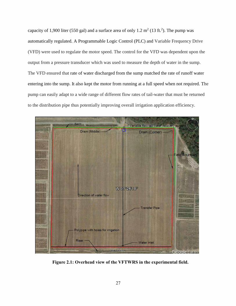
2.1 Details of the variable flow tail-water recovery system

This irrigation system was located at the University of Arkansas, Rice Research and Extension

Center, Stuttgart, AR. The field of study was a 16 ha (40 ac) graded slope (row rice) field. Rice

crop was primarily chosen for the study because it remains unaffected by waterlogging and thus

allows the opportunity for more irrigation events in comparison to other row crops in a growing

season. The system consisted of a small pumping unit which was installed at the bottom end of

the field. This pumping unit was used to recirculate tail-water collected at the bottom end of the

field into the same field. The outlet of the pump was connected to a transfer pipe (30 cm or 12 in

diameter & 20 mil poly-pipe) which ran along a furrow and was connected to a poly-pipe line

(10 mil) which was used to allow irrigation water into each furrow at the field (Figure 2.1). The

unit consisted of a stainless steel axial propeller pump which was installed in a sump with a

27

capacity of 1,900 liter (550 gal) and a surface area of only 1.2 m2 (13 ft.2). The pump was

automatically regulated. A Programmable Logic Control (PLC) and Variable Frequency Drive

(VFD) were used to regulate the motor speed. The control for the VFD was dependent upon the

output from a pressure transducer which was used to measure the depth of water in the sump.

The VFD ensured that rate of water discharged from the sump matched the rate of runoff water

entering into the sump. It also kept the motor from running at a full speed when not required. The

pump can easily adapt to a wide range of different flow rates of tail-water that must be returned

to the distribution pipe thus potentially improving overall irrigation application efficiency.

Figure 2.1: Overhead view of the VFTWRS in the experimental field.

28

2.2 Research objectives

The objectives for this study were to:

1. Evaluate the performance of the variable flow tail-water recovery system on electric

energy source (using conventional electric power from local utility grid (Grid) and solar

energy captured by PV modules (PV)).

2. Compare and contrast irrigation efficiencies of three different furrow irrigation systems-

conventional furrow irrigation system, surge irrigation and VFTWRS.

3. Determine the economic feasibility of the VFTWRS by comparing it to a conventional

tail-water recovery systems designed for the same field.

4. Evaluate crop yields and plant heights of different rice varieties in a furrow irrigated

field.

29

3. Materials and Methods

3.1 Description of study area

The Rice Research and Extension Centre is located in the Grand Prairie rice growing region in

Arkansas. With subsequent land additions each year since 1927, the RREC has now about 414 ha

(1,022 ac) of land for research in rice, soybean, etc. RREC, with USDA/ARS National Rice

Research Center alongside, is the well-known and largest rice research location in the US.

According to the Soil Survey of Arkansas County (NRCS 2005) the soil type in the Grand Prairie

(GP) region is mainly silty material at the top and red clayey material as the subsoil. The

prevalent soil types in the GP region are the Dewitt and Stuttgart soils. Average winter

temperature since 1971 is 6.7ºC (44º F) and daily average minimum temperature is 1ºC (34o F).

Average summer temperature is 26ºC (80o F) while the maximum daily temperature is 33ºC (91º

F). Arkansas receives annual precipitation of 124 cm (49 in) and the average snowfall is about 13

cm (5 in). Average rainfall of 94 cm (37 in) is expected between March and November. The

average relative humidity is 57 percent at mid-noon and about 84 percent at dawn. Observed

wind speed from February to April averages to 14.5 km/hr (9 miles/hr).

3.2 Hydrogeology

The total area of the field of study was approximately 16 ha (40 ac). According to the Web Soil

Survey (WSS), 92% of the total study area has DeWitt silt loam while the rest is Stuttgart silt

loam. The results from the WSS is shown in Figure 3.1.

30

Figure 3.1: Web Soil Survey result of the field of study on 10/5/2016 (The dots represent the

site of soil sampling for soil properties’ analysis).

Table 3.1: Web Soil Survey result of the field of study

Soil samples from 5 locations (shown in Figure 3.1) from the middle of the field equidistant from

top to bottom at different depths were also sent for textural, field capacity, wilting point, bulk

density and organic matter analysis to the American Agricultural Laboratory, Nebraska. The

results obtained from the soil tests are shown in Table 3.2.

Map Unit

Symbol

Map Unit Name Hectares (acres) in

Area of Interest

Percent of Area of Interest

3A Dewitt silt loam, 0 to 1 percent slopes 14.5 (35.9) 92.1%

23B Stuttgart silt loam, 1 to 3 percent slopes 1.25 (3.1) 7.9%

3A

23B

31

Table 3.2: Laboratory test results for the soil samples from the field of study

Site Depth (cm) Texture (%) OM, LOI Bulk

density

WP (v/v %) FC (v/v

%) Sand Silt Clay

1 (Top) 0-25.4 13 70 17 1.7 1.37 10.31 28.37

>25.4 cm 21 30 40 2.1 1.19 27.10 41.06

2 0-25.4 11 70 19 1.6 1.37 10.58 28.55

>25.4 in 21 30 40 2.1 1.19 27.10 41.06

3 0-25.4 13 70 17 1.8 1.34 10.81 28.83

>25.4 cm 21 30 40 2.1 1.19 27.10 41.06

4 0-25.4 13 68 19 1.8 1.33 10.51 29.45

>25.4 cm 21 30 40 2.1 1.19 27.10 41.06

5 (Bottom) 0-25.4 13 68 19 1.9 1.31 12.58 30.02

>25.4 cm 21 30 40 2.1 1.19 27.10 41.06

3.3 Experimental plot for variety study

Due to the presence of a compaction subsoil layer, the experimental field was deep tilled prior to

bed construction to a depth of 30 cm (12 in) perpendicular to the slope of the field with a 5-shank

no-till soil management system ripper (John Deere, Moline, IL) in the year 2016. Raised beds

were constructed on a 76 cm (30 in) spacing while the seeds were drilled at a 19 cm (7.5 in)

spacing along the furrows and beds. The dimensions of the plot for year 2016 were 386 m (1,265

ft) wide by 379 m (1,243 ft) long, area was 14.7 ha (36.3 ac), with slope of 0.2 m for every 100

m (0.2%) and 512 furrows. The dimensions of the plot for year 2017 were 386 m (1,265 ft) wide

by 384 m (1,260 ft) long, area was 14.8 ha (36.6 ac), with slope of 0.2 m for every 100 m (0.2%)

and 510 furrows. Experimental setup for both years, 2016 and 2017, were different. In 2016,

evaluation of continuous flow furrow irrigation (CFI), surge irrigation (SI) and furrow flow

irrigation with tail-water recovery using the VFTWRS was performed on the same experimental

plot. In 2017, furrow irrigation using VFTWRS was performed and power sources were changed

for different events from electric grid (VFTWRS-Grid) to solar PV modules (VFTWRS-PV). All

rice varieties were replicated three times in three blocks 1, 2 and 3 using Mermentau as the filler

32

rice crop in 2016 and Jupiter as the filler crop in 2017. Filler crop (F) was planted in 6 rows

between each replication block 1 & 2 and 2 & 3, respectively and on the sides as well as bottom

of the plot. Each variety was planted on twelve rows each. In 2016, 12 rows on either sides of the

plot were planted with XL 729 as filler and 24 rows on east side of the field were used for

Nitrogen (N) study which was followed by 20 rows of filler crop (Figure 3.3). In 2017, 144 rows

in the West side of the field were used for N Study with 7 rows of filler on the west side and 18

rows of filler on the east side (Figure 3.4). Experiments related to the N study are not presented

in the thesis.

Following rice varieties with the seeding rates were used for planting for the respective years

(Table 3.3). All varieties were direct seeded with a Great Plains 1500 drill with 19 cm (7.5 in)

row spacing across the raised beds and furrows.

Figure 3.2: Randomized block design for rice variety study, 2016

Figure 3.3: Randomized block design for rice variety and Nitrogen study, 2017

Rows 12 12 12 12 25 42

Tre

atm

ent

F

XP

75

6

Tit

an

Fra

nci

s

Dia

mo

nd

XL

74

5

Mer

men

tau

XL

72

9

Lak

ast

45

22

Jup

iter

10

99

F

Mer

men

tau

XL

74

5

Fra

nci

s

Jup

iter

Tit

an

Dia

mo

nd

45

22

XL

72

9

10

99

XP

75

6

Lak

ast

F

10

99

XL

74

5

XP

75

6

45

22

Dia

mo

nd

Jup

iter

Mer

men

tau

XL

72

9

Lak

ast

Tit

an

Fra

nci

s

F

N S

tud

y

F

Variety study

12×11 12×11

North

12×11

33

Table 3.3: Seeding rates for all rice varieties planted in the plots, 2016 and 2017

2016 2017

Varieties Seeding Rate

[kg/ha (lbs/ac)] Varieties

Seeding Rate

[kg/ha (lbs/ac)]

Titan

Co

nv

entio

nal

84 (75) CL 153

Co

nv

entio

nal

85 (76)

Francis 70 (63) CL 172 84 (74)

1099 72 (64) Jupiter 91 (81)

Jupiter 78 (70) Diamond 68 (61)

Diamond 69 (62) Gemini

Hy

brid

27 (24)

Mermentau 72 (64) RT XL753 29 (26)

RT XL753

Hy

brid

30 (27) RT CL 7311 29 (26)

RT XL729 27 (24) RT CL XP4534 32 (29)

RT XL745 27 (24) RT XP 754 34 (30)

RT XP756 29 (26) RT CL XL745 (N

Study) 31 (28)

4522 27 (24)

3.4 Field experiment management

A lay-flat pipe (Delta Plastics®, 30.5 cm (12 in) diameter, 0.25 mm (10 mil) thickness) was used

for irrigating the furrows. A universal hydrant was used to control the inflow of water from the

reservoir to the field. The position of the hydrant was almost in the middle of the field. A PVC T

was used to connect PVC pipeline from the hydrant to the 10 mil PVC pipeline (Figure 3.4).

Each hole of diameter 0.95 cm (3/8 in) was punched for each furrow. The appropriate diameter

of the holes was determined using Phaucet® (Version 8.2.20; NRCS, 2011) and Pipe Planner®

(Delta Plastics®, 2016) (Figure 3.5).

34

Figure 3.4: Universal hydrant is connect to a propeller flowmeter, a badger meter and a

pipeline which supplies water to the field

Figure 3.5: Screenshot of the design obtained from Pipe Planner for the experimental

plot.

Irrigation methods which were studied in the field were continuous flow furrow irrigation, surge

irrigation and variable flow tail-water recovery system in the year 2016. All the events were

applied in the same plot. The irrigation methods were randomly selected while the scheduling of

the irrigation events were done using GMS sensors. Generally, average number of days between

irrigation events was 3 days. These sensors are discussed later in detail. Average target irrigation

35

on-time which is the time the field is watered using irrigation was taken as 42 hrs. Average target

flow rate for continuous flow irrigation and tail-water recovery irrigation was taken as 50.5 l/s

(800 gpm) but in actual field conditions it varied from 47.3 l/s (750 gpm) to 63.1 l/s (1,000 gpm).

For surge irrigation, target flow rate was taken as 31.5 l/s (500 gpm) and was maintained as 31.5

l/s (500 gpm) throughout the irrigation period while for the last surge irrigation event it was kept

as 53.6 l/s (850 gpm). Ideally, the hole sizes for the surge irrigation events were supposed to be

larger (1.27 cm or 1/2 in) than the hole size for CFI events (0.95 cm or 3/8 in). This was not

possible due to usage of the same poly-pipe as in CFI events. However, for the last surge

irrigation event the holes sizes were increased to 1.27 cm (1/2 in).

In the CFI events, the runoff water generated from the fields was allowed to free drain after

desired water depth was applied. For surge irrigation events, the inline tee connecter was

replaced with a surge valve. The runoff water was allowed to free drain and irrigation was turned

off after desired depth was applied. In the case of VFTWRS, all the drains were blocked by

raising the inlet elevation of the drop pipe up to the level of the berm surrounding the field. The

runoff water, thus, was allowed to back up at the bottom of the field. Horizontal drain furrows

were constructed at the bottom of the field which some grade towards the tail-water recovery

sump. This allowed the tail-water to enter the sump. VFTWR pump was turned on from the start

of the event whose speed varied according to the depth of water in the sump. The inlet flow was

initially started with a flow rate similar to that of continuous furrow irrigation, the flow rate was

adjusted according to the flow rate of recirculated water from the VFTWR pump. The main

supply of water from the reservoir was turned off after bottom of the field was filled with tail-

water. This condition was usually possible after about 12 hrs since the start of the event.

36

For the year 2017, irrigation events using only the VFTWRS were conducted. However, the

energy source to run the system was changed to either electric or solar. For the electric VFTWRS

all the events were managed the same way as they were in 2016. For solar VFTWRS, the

irrigation events were started at night and the inflow was cutoff in the morning. This was done in

order to ensure that there was enough tail-water generated by morning so the daylight hours

could be utilized to power the system using solar energy.

3.5 Crop management

In 2016, the crop varieties were planted on May 13 which was followed shortly by an application

of Diammonium Phosphate (DAP) and Zinc. Herbicides, Facet and Command, were applied 20

days and 38 days after planting according to labeled rates. Two applications of Urea with

Agrotain were applied on June 9 and June 23 at the rate of 57 kg/ha (50 lbs./ac) and then 111

kg/ha (100 lbs./ac) of Nitrogen. One application of Ravage (Innvictis, Loveland Colorado) was

applied on August 13. The middle 6.1 m (20 ft) of each plot was harvested using a 1620 Case

International Combine (CNH Industrial, London, UK) between September 16 and September 17.

Out of 32 rows in each plot, 16 middle rows of each rice variety plot were harvested.

In 2017, the planting was completed on May 11-18. Three herbicide treatments were done in that

year (7th, 32nd and 93rd days from the planting day). The first treatment was done with Command

and League, the second treatment with Facet, Stam, Permit Plus and COC and the third with

Clincher and RebelX according to their labelled rates. Sixty eight kg (150 lb) of N was applied in

the variety study by splitting it into 84 kg/ha (75 lb/ac) applications each on 33rd and 50th day

from the planting day. One application of MustangMax was applied for stinkbugs on August 23.

37

Harvesting for variety plots was completed by September 22. All the herbicide, pesticide and

fertilizer treatments done into the experimental plot is shown in Table 3.4.

Table 3.4: Treatments done on the rice field in 2016 and 2017

2016 2017

Planting date 13 May Planting date 11-18 May

DAP and Zinc application 13 May Herbicide application 18 May

Herbicide application 2 June Herbicide application 12 June

Urea application 8 June Urea application 13 June

Herbicide application 20 June Urea application 29 June

Urea application 22 June Herbicide application 11 August

Pesticide application 13 August Pesticide application 23 August

Harvesting date 16-17 September Harvesting date 10-22 September

3.6 Variables measured in the field

3.6.1 Soil moisture potential and irrigation scheduling

One of the important factors for determining the adequacy of an irrigation event is by looking at

soil moisture content in the root zone of the soil (Davila et al., 2012). Soil moisture tension can

also be used to determine soil moisture condition in the root zone. Soil water potential and soil

water content are related to each other and can be represented using relationship similar to the

one shown in Figure 3.6 (Bilsie, 2001).

38

Figure 3.6: Generic soil water characteristic curves for each soil type (Bilsie, 2001)

Soil moisture potential in experimental plots were measured using Granular Matrix Sensors

(GMS) (Watermark Sensors®, Irrometer, CA) and were installed at varied depths throughout the

field. These sensors are solid state electrical resistance sensing devices which are used to

measure soil water tension. Sixty-four GMS sensors were installed in the field in three equally

spaced rows to measure moisture tension readings at different depths. Each row was termed as E

(for East), W (for West) and M (for middle). In each row, five GMS stations were installed

equidistantly at location 1, 2, 3, 4 and 5 (Figure 3.7). Each GMS station consisted of 4 sensors at

10 cm (4 in), 15 cm (6 in), 30 cm (12 in) and 60 cm (24 in) of depth and were installed at five

equally spaced locations along each of the three rows in 2016. The sensor depths were 10 cm (4

in), 15 cm (6 in), 30 cm (12 in) and 46 cm (18 in) for year 2017. Irrigation scheduling was

determined by another GMS station installed at bottom 1/3rd of the field. This station was

connected to a soil moisture monitor (AgSense, AquaTrac®, Huron, SD) which was monitored

daily.

39

Figure 3.7: Position of GMS stations in the field for moisture tension measurement (Blue

dots represent position of GMS stations)

3.6.2 Water advance time over furrow surface:

Advance time is the number of hours needed for water to travel from the delivery point to the

lower end of a field. Long advance time could mean uneven distribution of water in the field and

higher deep percolation and therefore, shorter advance time is desirable (Kranz et al., 2015). In

the experimental plots, advance time was measured by determining the advanced length of water

in the furrow and the time since the start of irrigation. The border rows of the field were flagged

at every 30 m (100 ft) to make estimates of distance travelled by the water front from the top of

the furrow. The elapsed time was determined using a stop watch by the researcher. Advance

front was observed four to five times for each irrigation event. Each time, 20-25 random furrows

were observed to record length of advance front and time elapsed. The final readings were

determined by taking average of these observations.

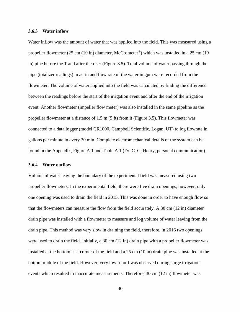
40

3.6.3 Water inflow

Water inflow was the amount of water that was applied into the field. This was measured using a

propeller flowmeter (25 cm (10 in) diameter, McCrometer®) which was installed in a 25 cm (10

in) pipe before the T and after the riser (Figure 3.5). Total volume of water passing through the

pipe (totalizer readings) in ac-in and flow rate of the water in gpm were recorded from the

flowmeter. The volume of water applied into the field was calculated by finding the difference

between the readings before the start of the irrigation event and after the end of the irrigation

event. Another flowmeter (impeller flow meter) was also installed in the same pipeline as the

propeller flowmeter at a distance of 1.5 m (5 ft) from it (Figure 3.5). This flowmeter was

connected to a data logger (model CR1000, Campbell Scientific, Logan, UT) to log flowrate in

gallons per minute in every 30 min. Complete electromechanical details of the system can be

found in the Appendix, Figure A.1 and Table A.1 (Dr. C. G. Henry, personal communication).

3.6.4 Water outflow

Volume of water leaving the boundary of the experimental field was measured using two

propeller flowmeters. In the experimental field, there were five drain openings, however, only

one opening was used to drain the field in 2015. This was done in order to have enough flow so

that the flowmeters can measure the flow from the field accurately. A 30 cm (12 in) diameter

drain pipe was installed with a flowmeter to measure and log volume of water leaving from the

drain pipe. This method was very slow in draining the field, therefore, in 2016 two openings

were used to drain the field. Initially, a 30 cm (12 in) drain pipe with a propeller flowmeter was

installed at the bottom east corner of the field and a 25 cm (10 in) drain pipe was installed at the

bottom middle of the field. However, very low runoff was observed during surge irrigation

events which resulted in inaccurate measurements. Therefore, 30 cm (12 in) flowmeter was

41

replaced with a 20 cm (8 in) flowmeter. Clogging of the propeller caused by biological mass was

observed during some irrigation events. Regular cleaning of flowmeters were ensured during the

irrigation seasons.

3.6.5 Yield of rice crop

A commercial combine (model 1620 Case International, Grass Island, NE) and a 6.1 m (20 ft)

rice header were used to harvest the crop on September 16-17, 2016 and September 14-22, 2017.

Out of 32 rows in each plot, 16 middle rows of each rice variety plot were harvested. The

harvested rice was weighed in a calibrated weigh-wagon. A total of 33 rice plots (eleven rice

varieties in three replications) were harvested in 2016. In 2017, 27 rice variety plots and 12 N

study plots were harvested. The plot length was measured using a wheel distance measuring

gauge (Rolatape®, Watseka, IL) while the plot width (W) was the same as the length of rice

header (6.1 m or 20 ft). Length of harvested plot (L), harvest weight (W), gain moisture (MC),

and plant heights were recorded at the time of harvest. The harvest weights were corrected with a

12% moisture correction using the measured grain moisture from each plot using the following

formula,

WMC = W ×(100−MC)

(100−12) (2)

where, WMC= moisture corrected weight, %v/v

W= harvested weight

MC= moisture content of the harvested weight sample.

42

Yield was calculated as,

Yield =WMC

A (3)

where, WMC= moisture corrected weight

A= area of the harvested plot.

3.6.6 Plant height and growth stage

Plant heights were measured using a wooden graduated scale with a least scale of 0.25 cm (0.1

in). The scale was placed next to the plant and the height was measured from the bottom of the

plant to the top of the plant. For each plot, the plant height was measured at the top (1/3rd of field

length), middle (1/3rd to 2/3rd of field length) and bottom (bottom 1/3rd of the field length) of the

field length. For each block, heights of 8-10 randomly selected plants were measured at the beds

and furrows and their average was recorded. The rice growth stages were determined according

to the Arkansas Rice Production Handbook (Moldenhauer et al., 2013). Reproductive growth

stage of different rice varieties for each replication were recorded in mid-August for both years.

Random plants were selected in the middle of the rice plots to observe the growing stage of the

crop.

3.7 Estimated variables

3.7.1 Deep percolation and evapotranspiration

The GMS sensor readings were monitored at different depths (10 cm, 15 cm and 30 cm) in order

to estimate deep percolation. The root zone of the crop was determined by inspection between 25

cm (10 in) to 36 cm (14 in). In theory, field capacity is the amount of water remaining in a soil

when the downward water flow due to gravity becomes negligible (Lo et al., 2017). Therefore,

43

the deep percolation losses were taken as 0 when the values of the bottom most sensors at 30 cm

(12 in) were above field capacity (33 cb). Deep percolation losses were also considered to be 0

when values of bottom most sensors were observed to be increasing during the irrigation events.

This indicated a decrease in soil moisture content and hence deep percolation was considered 0.

For the rest of the events, the following water balance equation was used (Hatiye et al., 2016):

DPi = ∑ (θi−1 − θi)jnj=1 + Pi + Ii − ETci − Ri (4)

where, P = precipitation

I = applied irrigation

ETc = actual evapotranspiration

DP = deep percolation of water moving out of the root zone

R = surface runoff

i and i – 1, respectively = the current and previous time steps (days in this study).

θ = soil moisture content (%) in the root zone depth

j= individual root zone interval.

Moisture content at i and i-1 time periods were calculated by converting the moisture tension

readings obtained from GMS sensors to v/v % using soil water characteristics equation (Saxton

and Rawls, 2006).

Average readings from the sensors at 4 in and 6 in were used to represent moisture tension in the

top 25 cm (10 in) of the root zone. Readings from the sensor at 30 cm (12 in) was used to

represent moisture tension from 25 cm (10 in) to 36 cm (14 in) of the root zone. Water balance

calculations at each of the 15 GMS stations were performed where one station represented 1 ha

(2.5 ac) of area. The deep percolation values were calculated for all of the 15 GMS stations.

44

These values were then averaged to obtain DP for the whole field. Similar calculations were

done for all of the irrigation events for both years (Tables A.14 and A.15). Evapotranspiration

was estimated using weather station data was used to calculate grass reference ET. University of

Idaho ET software Ref-ET® was used to calculate FAO 56 Penman-Montieth grass reference ET

using parameters max/min air temperature, wind speed, average solar radiation, precipitation and

max/min relative humidity. The crop coefficients to calculate crop ET for rice were obtained

from Vories et al. (2013) study on sprinkler rice (Figure 3.8).

Figure 3.8: Crop coefficient values for sprinkler irrigated rice (Vories et al., 2013)

3.7.2 Irrigation efficiency and water use efficiency

Irrigation efficiency is defined as the ratio of beneficially used irrigated water and total applied

water. Beneficially used water is calculated by subtracting non beneficial uses from total applied

water. These non-beneficial uses include soil evaporation, deep percolation and tail-water (Burt

et al., 1997). For the experimental studies zero soil evaporation was assumed. Irrigation

efficiency can be represented by the following equation (Burt et al., 1997):

Irrigation Efficiency, IE =Beneficially used irrigated water

(Beneficially+Non−beneficially)used irrigated water (5)

WUE was calculated as bu/ac-in/ac by dividing yield per acre of each plot by water used (ac-

in/ac) throughout the irrigation season by the plot (Gaspar et al., 2016).

45

3.8 Pump testing

In order to find optimum operating conditions for the pump, pump testing of the developed

VFTWR pump was performed. As the first step a pump curve was created by plotting Total

Dynamic Head (TDH) against ‘pump discharge’, Q at different motor speeds ranging from 35 Hz

to 60 Hz. TDH is the sum of total static head, velocity head and friction head (USDE, 2006). Total

static head is the sum of suction lift and elevation lift, also known as discharge head. Velocity

head is generally ignored in TDH calculations because of their low values (Bernuth, 2015).

Pressure at the discharge end was measured using a watch glass PVC pipe which was connected

to the top of stand pipe. Suction lift was measured using a yard stick from water surface to the

datum (center line of discharge pipe). During pump testing, the discharge was varied and

corresponding suction lift and discharge head was noted. This test was performed for different

motor frequencies of 35, 40, 50 and 60 Hz. Discharge, Q from the pump was measured using

Krohne waterflux 3070 flowmeter and power consumption was measured using 434 Fluke power

quality analyzer. The pump curve was obtained by plotting total dynamic head against discharge

at different speeds. Pump efficiency and Water Horse Power (WHP) were determined using the

following equation (Kranz & Yontz, 2010):

ŋ𝑃 =WHP

BHP ×ŋ𝑀 (6)

where, ŋ𝑃= pump efficiency

WHP= water horsepower

BHP=brake horsepower

ŋ𝑀= motor efficiency

46

WHP =Q × TDH

3956 (7)

where, WHP= water horsepower

Q=discharge

TDH=total dynamic head

Pumping plant efficiency can be calculated once water power and energy consumption are

calculated, since there is a known ratio between work done by the pump system and total energy

consumption. This ratio is used to determine pumping plant performance relative to the

Nebraska Pumping Plant Performance Criteria. The NPPPC provides numerical values for

expected work done on the water by the pump per unit consumption over the same duration.

NPPPC benchmark values are given as a ratio of work (whp-hr) per unit of input energy. The

NPPPC for electric pumps is 0.885 whp-hr/kW-hr (Kranz and Yontz, 2010).

% of NPPPC =

whp−hr

Unit of power consumed

NPPPC (8)

% of NPPPC was also calculated during the irrigation season. The parameters for the

calculations were automatically logged on the Campbell scientific logger. The TDH was evaluated

as follows,

TDH = (Length of airline sensor tube − Head from airline sensor) +Elevation from top of airline sensor tube to datum + Discharge head +

Elevation from datum to water outlet (9)

Due to low values of discharge head, the pressure transducer installed at the stand pipe was unable

to report any readings. For the year 2017, the PVC relief connected to the standpipe was replaced

with another PVC relief which was installed with an 81 cm (32 in) long Milone eTape® liquid level

sensor in order to record discharge head. However, the liquid level sensor was corrupted after a

few days due to poor construction of the sensor. In order to estimate discharge head, a relationship

between frequency of pump, Hz and discharge head was calculated from the data when the liquid

47

level sensor was in working condition. Following logarithmic relationship (R2=0.824) was the best

fit relationship obtained from the data,

Discharge head, in = (39.1088 ∗ Ln(Frequency, Hz)) − 118.95 (10)

This relationship was then used to estimate discharge head for all events in 2016 and 2017. An

exponential relationship between the two overestimated discharge head for frequencies > 40 Hz.

Although the equation underestimated discharge head for frequencies less than 19 Hz, the

efficiency analysis was conducted for data greater than 20 Hz. The power consumption, speed of

the motor, current and voltage used by the pump, discharge from the pump were collected by

CR1000 and MD485 using MODBUS communication with the VFD.

3.9 Solar analysis

The VFTWRS can be operated with solar energy by connecting it to PV modules. For some

irrigation events during the irrigation season in 2017, the pump was operated using the energy

generated from the Monocrystalline silicone PV modules (Mitsubishi Electric Photovoltaic

module, Model: PV-MLE265HD, maximum power= 265W).

The % of NPPPC for the solar powered system was calculated the same way as described in the

pump testing section. In order to decrease the payback period of the solar panels, the panels were

designed to be mounted on a portable trailer so they could be connected to the utility grid via

inverter to obtain net metering credit in the offseason. The potential average power generated per

month from the panels was estimated by using average solar irradiance data for each month for

10 years from 2008 to 2017. This solar irradiance data was obtained from the weather station at

the RREC, Stuttgart AR. This information was used to find a relationship between solar

irradiance and energy generated from panels which was then eventually used to estimate average

48

energy for each month. For the months of March to June, the PV Modules were connected to an

inverter and a DENT instruments ELITEproXC power meter to record voltage, current and

power generated from the PV modules. For these months the PV modules were facing South at a

tilt angle of 150. For the period from July to September the panels were connected to the

VFTWRS and for these months the panels were facing South at a tilt angle of 450. The distance

between the location of the PV Modules and the weather station was 1.38 km (0.86 miles). The

instrument used to measure the solar irradiance was the CS300 apogee pyranometer. The area of

panels was 17.5 m2 (188 ft2) and the rated module efficiency was 16%. The relationship between

estimated energy generated from the panels and actual energy generated from the panels was also

obtained. The estimated energy from the panels was obtained as,

Estimated energy (kWh) = Hourly solar irriadiance (kW

m2 ) × Area of panels (m2) ×

Module efficiency (%) (11)

3.10 Economic analysis

To determine the economic feasibility of the developed variable flow tail-water recovery system,

a number of different possible tail-water recovery scenarios were studied. The scenarios included

conventional tail-water designs, variable flow tail-water recovery designs operated with PV

modules as well as with grid power available at different lengths. Case studies were performed

for all of these scenarios for a similar field by the researcher. Since the source of irrigation water

can be from two sources, well and surface water, all scenarios were studies for both of these

sources. Each base scenario was designed in AutoCAD Civil 3D (Figures A.2 to A.7) and their

capital and operating costs were identified. Water balancing for each scenario was conducted

using data from irrigation events which were performed on the field for years 2016 and 2017.

49

Annual irrigation water use and volume of water recirculated from these tail-water recovery

systems were estimated from the water budgets. These values were used to evaluate cost of

pumping from the irrigation water source and for the tail-water recovery pump. Costs involving

field preparation, chemical/fertilizer application, farm machinery and seeds remained constant

for all scenarios. Annual operating costs were determined using 2017 row rice budget using

inputs from water budgeting for each scenario (Table 4.9). Capital costs for tail-water recovery

systems with ditches were evaluated using 2016 cost data available from NRCS (Table A.8). The

Net Present Value (NPV) approach was chosen for the analyses because it allows the

consideration of projects with different risk profiles and doesn’t involve setting an explicit

arbitrary threshold such as a minimum rate of return or a maximum pay-back time (Gaily, 2011).

NPV of estimated returns to land and profit generated from rice production were projected over

25 years (from 2017-2041) of time period on a per hectare basis.

NPV is the method to estimate net returns at one point in time using discounting formula of a

series of projected returns (Barry et al., 1983). Discount rates of 4%, 5%, 6%, 7%, 8% and 9%

were used for NPV calculations.

NPV = −INV + ∑Pn

(1+i)n25n=1 (12)

where, INV= system cost for each scenario in $/ha ($/ac)

Pn=net returns in $/ha ($/ac)

i=discount rate

Simple payback period as well as discounted payback periods were calculated for each of these

scenarios for discount rates of 4%, 5%, 6%, 7%, 8% and 9%. Simple payback period approach

assumes annual cost to remain the same over time and does not account for the time value of

money (Hofstrand, 2013). It is calculated as,

50

SPP =INV

P (13)

where, P=annual estimated net return per acre

The discount payback period (DPP) is the amount of time required for the cumulative present

value of operating costs to equal the cost of the irrigation system (Henry et al., 2016).

DPP = q +|CPVq|

CPVq+1= q +

|∑ PVqqy=1 |

|∑ PVq+1q+1y=1 |

(14)

where, q=last period (year) with a negative discounted cumulative present value (or CPV)

ǀCPVqǀ= absolute value of cumulative present value at time period q

ǀCPVq+1ǀ= absolute value of cumulative present value at time period q+1

Rice variety (XL753) and yield were assumed to be similar for all the scenarios. The results

obtained from rice variety studies indicated that XL753 had highest yield for both years 2016

and 2017 (explained in Section 4.7.1), hence, it was chosen as the crop for the analyses. The crop

was assumed to be continuously grown for each scenario. The yield results from 2017 rice

variety experiments were taken in the calculations which was 9,533 kg/ha (189 bu/ac) for XL-

753.

3.10.1 Water budgeting for simulated tail-water recovery systems

Water budgeting was done for each event using the data from irrigation efficiency experiments

for each year, 2016 and 2017. Before the start of the irrigation season, the tail-water pit was

assumed to be completely full from rain events prior to irrigation. For tail-water recovery events

with pit, net irrigation water applied to the field was calculated by adding water supplied from

the irrigation water source and total water recirculated by the VFTWRS. This data was obtained

from experiments conducted in both years at RREC. For each event, use of tail-water in the pit

was maximized. A small volume of 8.24 to 10.3 ha-cm (4 to 5 ac-in) of water was estimated to

51

be non-pump able to avoid cavitation. If volume of water in the pit was insufficient to complete

an irrigation event then irrigation water from other sources were used. For each irrigation event

and rainfall event, runoff was collected in the tail-water pits. Runoff volume exceeding the

capacity of the pits was allowed to drain from the pit as overflow. Runoff from irrigation events

was calculated by applying the water balance equation 4.

Runoff from rainfall events were calculated by using SCS Curve Number method for Hydrologic

soil group C. Curve number of 85 was used for agricultural lands of straight row crops of a good

condition (Huffman et al., 2013). Evaporation loss from soil was assumed to be negligible,

however, evaporation from pits were considered in the water balance equation. It was obtained

from mean monthly free water surface evaporation from the station Neptune, TN for the months

of June, July and August (USDA, 1992). Evaporation volume from the pit was calculated by

using a formula for a trapezoidal prism for the identified evaporation depth in the previous step.

Deep percolation and precipitation data obtained from field experiments were used for the

respective years. Irrigation events for solar powered tail-water recovery events were managed in

a different way. Therefore, water budgeting for these systems was slightly different than tail-

water recovery systems with pits. Solar radiation data was used to estimate energy generated by

the solar panels which was in turn used to estimated volume of tail-water pumped from the

pumping system for each irrigation event. Irrigation events were started at night and the water

was supplied from a nearby water source at the start of the event. After 7 AM, irrigation water

from nearby source was shut off and VFTWRS pumping system was allowed to recirculate tail-

water during the day using PV modules. Runoff generated from irrigation and rainfall were

allowed to collect at the bottom of the field for the VFTWRS to recirculate. Drain plugs were

never opened for these events. Additional irrigation water into the field was added after low

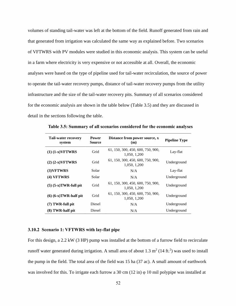
52

volumes of standing tail-water was left at the bottom of the field. Runoff generated from rain and

that generated from irrigation was calculated the same way as explained before. Two scenarios

of VFTWRS with PV modules were studied in this economic analysis. This system can be useful

in a farm where electricity is very expensive or not accessible at all. Overall, the economic

analyses were based on the type of pipeline used for tail-water recirculation, the source of power

to operate the tail-water recovery pumps, distance of tail-water recovery pumps from the utility

infrastructure and the size of the tail-water recovery pits. Summary of all scenarios considered

for the economic analysis are shown in the table below (Table 3.5) and they are discussed in

detail in the sections following the table.

Table 3.5: Summary of all scenarios considered for the economic analyses

Tail-water recovery

system

Power

Source

Distance from power source, x

(m) Pipeline Type

(1) (1-x)VFTWRS Grid 61, 150, 300, 450, 600, 750, 900,

1,050, 1,200 Lay-flat

(2) (2-x)VFTWRS Grid 61, 150, 300, 450, 600, 750, 900,

1,050, 1,200 Underground

(3)VFTWRS Solar N/A Lay-flat

(4) VFTWRS Solar N/A Underground

(5) (5-x)TWR-full pit Grid 61, 150, 300, 450, 600, 750, 900,


(6) (6-x)TWR-half pit Grid 61, 150, 300, 450, 600, 750, 900,


(7) TWR-full pit Diesel N/A Underground

(8) TWR-half pit Diesel N/A Underground

3.10.2 Scenario 1: VFTWRS with lay-flat pipe

For this design, a 2.2 kW (3 HP) pump was installed at the bottom of a furrow field to recirculate

runoff water generated during irrigation. A small area of about 1.3 m2 (14 ft.2) was used to install

the pump in the field. The total area of the field was 15 ha (37 ac). A small amount of earthwork

was involved for this. To irrigate each furrow a 30 cm (12 in) φ 10 mil polypipe was installed at

53

the top of the field and a 0.95 cm (3/8 in) φ hole was punched for each furrow in the polypipe.

The water from the pump was returned to the polypipe at the top using a thicker 12 mil 30 cm

(12 in) φ polypipe. A power line of 61 m (200 ft) was connected from the power source to the

pump. Energy consumption for VFTWRS system was estimated from the experimental data

obtained for the year 2017. The storage for tail-water at the bottom of the field was about 44 ha-

cm (1.8 ac-ft). A total of 2 drain pipelines were deemed sufficient for drying the field for

harvesting. The grade of the field as well as the drain pipeline was 0.2%. This design was similar

to the VFTWRS which was used in the irrigation efficiency analysis. The total amount of water

used for this scenario was identified from the field experiments on irrigation efficiency

conducted in 2016 and 2017 at Rice Research and Extension center, Stuttgart.

3.10.3 Scenario 2: VFTWRS with underground pipeline

This system was designed similar to Scenario 1 except one change in the design. The transfer

pipe was used to recirculate tail-water from the bottom of the field to the top was replaced with a

permanent irrigation pipeline of similar length. This change in the system increased the capital

cost of the system while the annual operating cost of the system remained the same as in

Scenario 1.

3.10.4 Scenario 3: VFTWRS with lay-flat pipeline using solar panels

The design for this scenario was the same as the one above except for the power source. A

portable solar panel structure was constructed to hold 12 PV modules. Each module was 1.63 m

(64 in) by 1 m (40 in) in area and had a maximum power rating of 265 W (Mitsubishi PV-

MLE265HD). Two portable structures each 1.83 m (6 ft) by 6 m (20 ft) was designed to hold 6

PV modules for each structure. Each module was able to pivot along its middle axis

(perpendicular to its length) which was able to provide angle adjustments for the panels for

54

different seasons throughout the year. A Fronius Galvo 3.1-1 inverter was used to convert

variable DC output from the PV modules into a utility frequency AC for the pump. The panels

were used as a power source for the pump during the months of irrigation, May to August. For

the rest of the months, September to April, the panels were connected to the public utility power

grid to obtain credit under the Arkansas net metering law. Any gain in revenue from net metering

credit was taken as a monetary benefit for NPV analysis.

3.10.5 Scenario 4: VFTWRS with underground pipeline with solar panels

This system was designed similar to Scenario 3. The water balance was similar to that in

Scenario 3. The transfer pipe used to recirculate tail-water from the bottom of the field to the top

was replaced by a permanent irrigation pipeline.

3.10.6 Scenarios 5/7: Tail-water recovery full width (electric and diesel pump)

This system was designed on the same field for a tail-water recovery system. A standardized

TWR ditch dimensions from NRCS were used to construct a tail-water ditch along the bottom

width of the field. The total length of the ditch was about 384 m (1260 ft) and surface area taken

by the ditch was 0.97 ha (2.4 ac). The ditch was designed according to a cut to fill ratio of 1.2: 1.

A total of five drain pipelines were included in the design from the ditch to the drain trench. The

inlet of each drain was set 0.3 m (1 ft) below the highest elevation of the ditch for any

overflowing rain or irrigation events. An L-drop was also constructed within the ditch to mount a

tail-water recovery pump. Scenario 5 consisted of electrical tail-water pump while scenario 7

consisted of diesel operated tail-water pump. Total area of the ditch was 0.97 ha (2.4 ac) which

reduced the total area of the field to 14 ha (34.6) ac. Opportunity cost from the 0.97 ha (2.4 ac)

land used for the construction of ditch was considered in the NPV analysis. The outlet of the

55

pump was connected to the irrigation water inlet into the field using an irrigation pipeline. Tail-

water storage of 207 ha-cm (8.4 ac-ft) was provided by the ditch.

3.10.7 Scenarios 6/8: Tail-water recovery half width (electric and diesel pump)

This system was designed for the same experimental field for a tail-water recovery system with a

ditch along the bottom of the field for half of its width. The total length of the ditch was 215 m

(706 ft) and area was 0.5 ha (1.2 ac). Opportunity cost from this 0.5 ha (1.2 ac) land which was

used for the ditch was considered in the NPV analysis. The total area of the field available for

production was 14.5 ha (35.8) ac. The design of the rest of the field was the same as in Scenario

5. Tail-water storage of 123 ha-cm (5 ac-ft) was provided by the ditch. Two types of tail-water

recovery pump was considered for Scenarios 6 and 8. Scenario 6 consisted of electrical tail-water

pump while scenario 8 consisted of diesel operated tail-water pump.

3.10.8 Scenarios (1, 2, 5, 6)-x foot: VFTWRS and conventional tail water recovery at

different distances form the grid power source

These scenarios were the same as Scenario 1, 2, 5, 6 except that the length of electrical wire from

the electrical supply to the tail-water pump was raised to x distance. The distances between the

pump and the utility service connections were 150 m (500 ft), 300 m (1,000 ft), 450 m (1,500 ft),

600 m (2,000 ft), 750 m (2,500 ft), 900 m (3,000 ft), 1,050 m (3,500 ft) and 4,000 ft (1,200 m). It

is important to note that the electrical wire up to length 600 m (2,000 ft) was an Aluminum 4

quad wire whose installation cost was $3.38/m ($1.03/ft), that between 600 m (2,000 ft) and 960

m (3,150 ft) was a 2 Quad Aluminum wire whose installation cost was $4.23/m ($1.29/ft) and

that between 960 m (3,150 ft) and 1,524 m (5,000 ft) was an Aluminum 1/0 quad wire whose

installation cost was $5.61/m ($1.71/ft). The length and quad of the electrical wire were

determined based on the amperage need of 3 hp motor and 3% voltage drop using a Paige®

56

agwire electric slide rule. With an increase in length of power source to the location of the

pumping system, the cost of the system also increased. It was important to account for different

lengths from power source to the pumping system because each farm is different in design and

values like these can play a big role in determining feasibility of irrigation systems.

57

4. Results and Discussion

4.1 Irrigation efficiency results for 2016

Each irrigation event was different from each other due to differences in soil moisture condition,

rainfall occurrences and availability of irrigation source. Each event has been described below in

detail. Irrigation efficiency, runoff, deep percolation, rainfall, tail-water ratio and water

application are tabulated in Table 4.1. Advance curve and hydrographs for all the events are

presented in Figure 4.1 and 4.2, respectively. Water balance conducted to estimated deep

percolation is provided in Table A.14.

a. Irrigation 1: CFI

The first irrigation (continuous irrigation) of the season was started on June 10 (planting date

May 13) which was 28 days after planting at about 3-4 leaf stage. The inflow was started at

about 49 l/s (775 gpm) which then slowed down to about 41 l/s (650 gpm) due to interrupted

supply of water at the experiment location. The advance time for this event was about 14 hours

and a very low runoff volume was generated from the irrigation. The field was deep tilled to 46

cm (18 in) prior to planting which may have helped in increasing the infiltration rate of the soil

resulting in a low runoff water. An irrigation efficiency of 83% was observed for the event. The

irrigation was followed by a rain event and the runoff water generated from the rain was allowed

to drain from the field. The plot was able to capture 1 cm (0.4 in) of rain from a total

precipitation of 1.7 cm (0.66 in).

b. Irrigation 2: CFI

A second event (continuous furrow irrigation) was started on June 19. The inflow of about 52 l/s

(825 gpm) was maintained throughout the event. The advance time for this event was 11 hours.

The irrigation, however, had to be stopped before the target application depth of 3.8 ha-cm/ha

58

(1.5 ac-in/ac) was achieved. This was done to avoid any drainage of herbicides from the field

which was to be applied the next day. The total time for this irrigation was about 31 hours. An

efficiency of 95% was achieved from this event, however, this event was discarded as a true

irrigation event due to insufficient target depth application.

c. Irrigation 3: CFI

This event was started on June 23 as a continuous furrow irrigation method. A constant inflow of

44 l/s (700 gpm) was maintained throughout the irrigation event. The advance time for the event

was 10 hours while an increase in runoff volume was observed after 30 hours. The event lasted

for about 45 hours and the efficiency was calculated to be 73%.

d. Irrigation 4: SI

This event was the first surge irrigation event for this growing season and was started on June 29

with an inflow of 38 l/s (600 gpm). The advance time for this event was 12.5 hours. This event

took 60 hours to apply the target application depth. Due to inability to increase furrow flow rates

for surge cycles, it took longer to apply required irrigation depth to the whole field. Uneven

distribution of furrow holes on both sides of the valve resulted in different furrow flow rates for

the two sides. Left cycle of the surge valve covered 60% of the total field area while the right

cycle covered 40% of the total field area. An application efficiency of 94% was achieved in this

event.

e. Rain

The runoff generated from this rain event on July 5 was allowed to leave from the field. A

rainfall capture of 0.86 cm (0.34 in) (94%) was calculated from the total precipitation of 0.91 cm

(0.36 in).

59

f. Irrigation 5: SI

This was a surge irrigation event which was started on July 7. The inflow was started at 28.4 l/s

(450 gpm). The advance time for this event was 9 hrs. A significant volume of runoff water was

observed to occur after 30 hrs from the start of the irrigation which was sooner in comparison to

the last surge irrigation event where significant runoff volume was observed after 42 hrs. This

irrigation resulted in a tail-water ratio of 0.18 which was 4.5 times higher than the last SI event.

The efficiency for this event was 81%.

g. Irrigation 6: VFTWRS-Grid

This event was the first VFTWRS event and it was also the first time of running the VFTWR

pump after the reinstallation of the pump. In the initial days there were some issues during the

pump operation like a leak in the bearing which took a couple of days to repair. Therefore, the

tail-water pump ran intermittently throughout the event. The inflow was started at 50 l/s (800

gpm) which was turned off after 11 hr just after the start of precipitation in order to capture and

recirculate tail-water from it. The advance time for this event was 8 hrs. Inflow was started again

after 35 hr after low tail-water volume was observed at the field’s bottom. It was also during this

time period that the readings of GMS sensors were close to 82 cb. Therefore, the event was

allowed to run for another 10 days continuously until GMS sensor readings came down to 0.

Total duration of this event was 11 days. During this period the event was managed by applying

water from the reservoir when the tail-water at the bottom of the field was insufficient. There

was a period during the event when the VFTWR was not functional which caused overflowing of

tail-water from the drains. This caused a runoff loss of about 1.2 ha-cm/ha (0.47 ac-in/ac). The

VFTWRS managed to recirculate 4.32 ha-cm/ha (1.7 ac-in/ac) of water while the water applied

from the reservoir was 9.9 ha-cm/ha (3.9 ac-in/ac) or 0.89 ha-cm/ha per day (0.35 ac-in/ac per

day).

60

h. Rain

This rain event occured on July 27 and the drains were were left open. A rainfall capture of 1.57

cm (0.62 in) was achieved while the total precipitation was 2 cm (0.8 in). Rainfall recovery for

this event was 77.5%.

i. Rain + VFTWRS-Grid

Total precipitation of 1.5 cm (0.60 in) occurred on July 30. For this event, the drains were

blocked and the VFTWRS was allowed to run on auto mode. A rainfall capture of 1.5 cm (0.59

in) (98%) was achieved and 1.37 ha-cm/ha (0.54 ac-in/ac) of rain water was recirculated.

j. Irrigation 7: CFI

This was a CFI event which was started on August 2. The inflow was started at 57 l/s (900 gpm).

The advance time for this event was 10 hrs and a large volume of runoff started to generate

immediately after the advance time. A total of 2.4 ha-cm/ha (0.95 ac-in/ac) of irrigation water

was lost as runoff and an efficiency of only 46% was achieved. A possible reason to explain this

event was the low infiltration rate of soil caused by a thin sealed crust which was observed at the

topmost layer.

k. Irrigation 8: VFTWRS-Grid

From previous VFTWR event’s data it was observed that keeping the initial inflow rate between

57 to 63 l/s (900-1000 gpm) caused higher runoff potential which allowed the VFTWRS to

complete irrigation within 40 hrs. The advance time for this event was 7.5 hrs. After about 17

hrs, inflow was turned off and VFTWR pump was turned on. In about 15 hrs, tail-water was

collected at the bottom of the field and the rest of the event was completed using the collected

tail-water. After 44 hrs, the target application depth was applied and the drains were unblocked

and remaining tail-water was allowed to drain from the field. While the tail-water was draining

61

from the field, rainfall occurred and the runoff for the event was estimated from hydrograph.

This event was 81% efficient. One of the reasons for its low efficiency than the other VFTWRS

events is that the VFTWR pump was not turned on in auto mode from the beginning of the event

and the inflow was not cut back after the advance time. This resulted in generation of runoff in

absence of runoff recirculation. This caused collection of runoff water at the bottom of the field

which was completely recirculated within 40 hrs of irrigation. However, it is anticipated that an

improvement in efficiency would have been observed if VFTWR pump was allowed to run from

the beginning and the inflow rate cut off after the advance time.

l. Irrigation 9: VFTWRS-Grid

This event was a VFTWRS event which was started on August 11. The inflow was started at 62

l/s (980 gpm) which was reduced to 39 l/s (620 gpm) after advance time of 10 hrs. This allowed

enough tail-water to be collected at the pump to be recirculated to compensate for this drop in

inflow. After 24 hrs, inflow was turned off and the remaining application was completed by the

recirculated tail-water. The drains were opened after 47 hrs into the event. An efficiency of 93%

was observed.

m. Irrigation 10: VFTWRS-Grid

This event was started on August 28 with an inflow of 59.94 l/s (950 gpm) which was then

reduced to 37.85 l/s (600 gpm) after 7 hrs. The advance time for this event was 11 hrs. By this

time tail-water was being re-circulated at 26.5 l/s (420 gpm) to compensate for the drop in

inflow. After 30 hrs, inflow was turned off and the drains were opened after 43 hrs. An

efficiency of 93% was achieved.

62

n. Irrigation 11: SI

For this surge irrigation event, all the holes in the polypipe were increased to a size of 1.27 cm

(1/2 in) from 0.95 cm (3/8 in). This was done in order to provide target application depth to the

field between 40-44 hrs. The inflow for the event was kept at 54 l/s (850 gpm) for both sides of

surge cycle. This increased the furrow flow rates for each side to 0.17 and 0.23 l/s (2.7 and 3.6

gpm) compared to the furrow flow rates of all other events which were in between 0.075 and

0.101 l/s (1.2 and 1.6 gpm). The runoff for this event started to generate after 7 hrs. This event

had the highest tail-water ratio of 0.66 and least efficiency of 32% compared to all other events.

In general, application efficiency started out high earlier in the season irrespective of the method

used. As the season progressed and soil sealing increased and water demand increased, efficiencies

for continuous flow and surge decreased from 83% and 94% to 46% and 32%, respectively.

However, tail-water recovery (TWR) remained highly efficient even at the end of the season

(93%). This data suggests that as the growing season progresses, irrigation efficiencies are

reducing the water supplied to rice plants at the time in the season when plant water demand is

highest for rice. This corresponds with sensor trends (Figure A.8) and suggests that monitoring of

soil moisture and taking steps to improve irrigation efficiency later in the season is needed to

improve water delivery to furrow irrigated rice.

63

Figure 4.1 (a, b, c, d, e, f): Advance curves for each irrigation and rainfall event for the

year 2016.

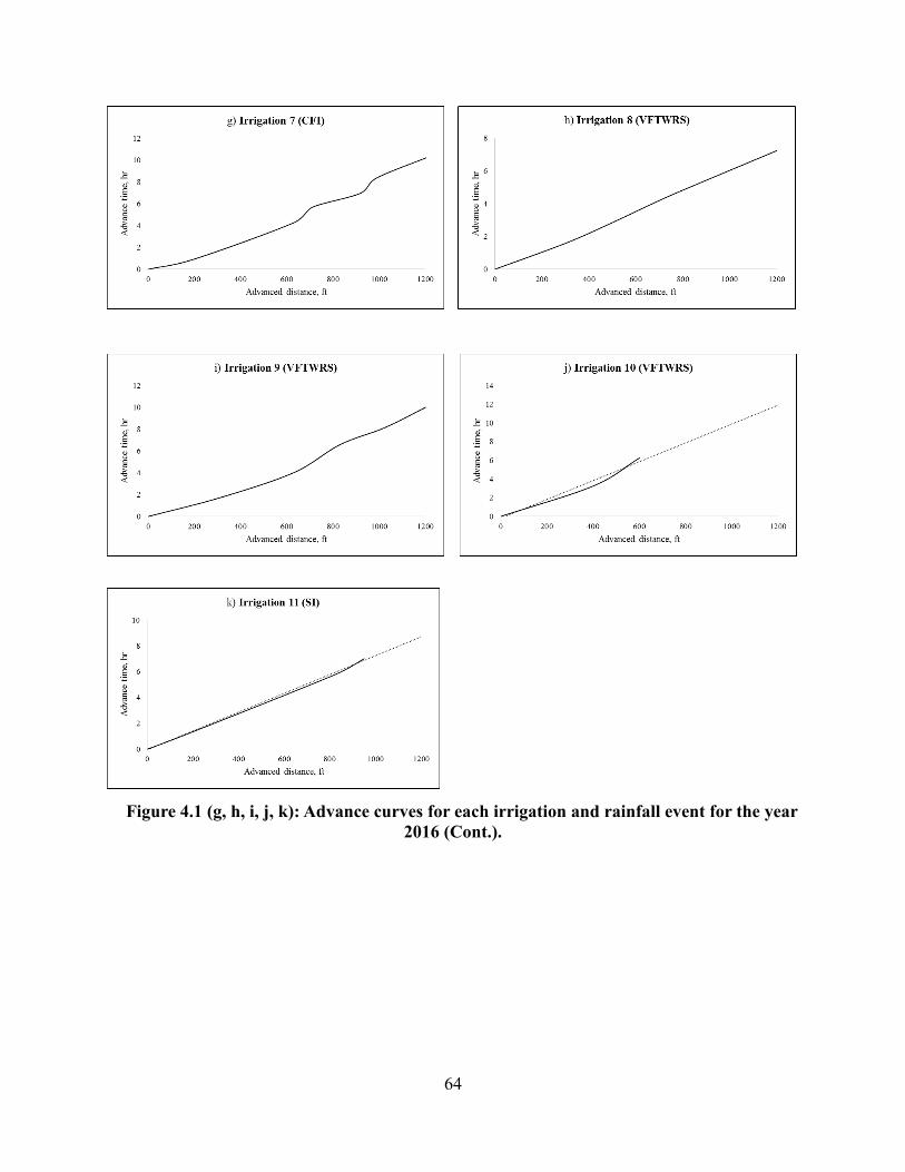
64

Figure 4.1 (g, h, i, j, k): Advance curves for each irrigation and rainfall event for the year

2016 (Cont.).

65

Table 4.1: Summary of all the irrigation and rainfall events for the year 2016

Irrigation/

Pptn. Date

Total

hours

Avg total

flow rate

(l/s)

Avg furrow

flow rate

(l/s)

Water

applied

(ha-cm)

Water

applied

(ha-

cm/ha)

Precipitat

ion (cm)

Runoff

(ha-

cm/ha)

Deep

Percolatio

n (ha-

cm/ha)

Water

recirculated

(ha-cm/ha)

Tail-

water

ratio

Irrigatio

n

efficien

cy (%)

Estimated

irrigation

efficiency w/o

VFTWRS (%)

Rainfall

capture

(cm)

CFI 6/10/2016 46 41.07 0.080 136 4.55 0.00 0.76 N/A 0 0.17 83 N/A 0

Precipitation 6/13/2016 N/A N/A N/A 0 0.00 1.68 0.66 N/A 0 0.4 N/A N/A 0

CFI 6/19/2016 31.3 52.74 0.103 119 3.96 0.00 0.10 0.11 0.00 0.03 95 N/A N/A

CFI 6/23/2016 45 43.09 0.084 140 4.67 0.00 0.84 0.42 0.00 0.18 73 N/A N/A

SI 6/29/2016 58 30.60 0.105 (W)

0.139 (E) 128 4.27 0.00 0.18 0.02 0.00 0.04 94 N/A N/A

Precipitation 7/5/2016 N/A N/A N/A 0 0.00 0.91 0.05 0.00 0.00 0.06 N/A N/A 0.81

SI 7/7/2016 51.7 28.39 0.097 (W)

0.129 (E) 106 3.53 0.00 0.66 0.00 0.00 0.18 81 N/A N/A

VFTWRS 7/14/2016 269 21.83 0.043 297 9.91 1.93 1.22 0.03 4.22 0.12 89 70 0.81



CFI 8/2/2016 36.7 51.74 0.101 137 4.57 0.00 2.41 0.04 0.00 0.53 46 N/A N/A

VFTWRS 8/5/2016 43.5 45.24 0.088 71 2.44 0.15 0.46 0.00 2.44 0.19 81 40 0.00


VFTWRS 8/11/2016 46.7 48.33 0.094 83 2.77 0.25 0.20 0.00 2.36 0.09 93 50 0.05

VFTWRS 8/28/2016 42 49.09 0.096 90 3.00 0.00 0.20 N/A 2.67 0.07 93.3 70 N/A

SI 9/1/2016 34.5 50.35 0.172 (W)

0.227 (E) 125 4.17 0.00 2.77 0.06 0.00 0.66 32 N/A N/A

Total 42 (Avg) 1,433 48 10 12 1 13 0.23 5

65

66

Figure 4.2 (a, b, c, d): Hydrographs for each irrigation and rainfall event for the year 2016.

a) b)

c) d)

66

67

a)

Figure 4.2 (e, f, g, h): Hydrographs for each irrigation and rainfall event for the year 2016 (Cont.).

e) f)

g) h)

67

68

Figure 4.2 (i, j, k, l): Hydrographs for each irrigation and rainfall event for the year 2016 (Cont.).

i) j)

k) l)

68

69

Figure 4.2 (m. n, o): Hydrographs for each irrigation and rainfall event for the year 2016 (Cont.).

m) n)

o)

69

70

4.2 Irrigation efficiency results for 2017

All irrigation events for this year were run on VFTWRS. The only parameter which was changed

in the events was the source of power to the system: solar energy from PV modules, electric

energy from electrical grid. Advance curves and hydrographs are presented in Figures 4.3 and

4.4, respectively while efficiencies are provided in Table 4.2. Water balance conducted to

estimated deep percolation is provided in Table A.15.

a. Irrigation 1: VFTWRS-Grid

It was observed from last year’s data that for VFTWRS events the initial inflow rate should be

about 57-63 l/s (900-1000 gpm) which should be cut off to about 38 l/s (600 gpm) after the

advance. The drains should be opened after target application depth has been applied. The first

irrigation of the season was started on 15th June, 30 days after planting. The inflow for the event

was variable for the whole event between 20 to 50 l/s (320 to 800 gpm). One of the pumps of the

pumping system in the station was damaged and only one pump system was used for all the

fields in the station which resulted in a low and inconsistent flow. During the night an inflow of

47 l/s (750 gpm) was available which was reduced to 25 (400 gpm) in the day. For this event, a

small amount of runoff water was generated and recirculated. An application efficiency of 93%

was achieved for the event.

b. Rain

This was a heavy rainfall event where a total precipitation of 9.98 cm (3.93 in) occurred. The

VFTWRS was allowed to run for the event although the precipitation was enough to fulfill the

irrigation requirement. Rainfall capture was about 5 cm (2 in) for the event, which was about

50% of the total rainfall.

71

c. Irrigation 2: VFTWRS-Grid

This event was started on June 30 at 50.47-56.78 l/s (800-900 gpm) of initial flowrate. No drains

were opened for this event and the end of the event was considered when almost all of the tail-

water at the bottom of the field was recirculated. Therefore, there was no runoff observed for this

event. The irrigation supply of the station was still being managed with one pump and the inflow

at the study field was not always consistent but it was stable for the most part. The VFTWR

pump had stopped due to inadequate tail-water in the sump after about 40 hrs and this was

considered as the end of irrigation. On 3rd July, a total precipitation of 0.43 cm (0.17 in) occurred

and only 0.54 ha-cm (0.26 ac-in) of tail-water was recirculated.

d. Irrigation 3: VFTWRS-Grid

This event was initiated on July 7. There was already some tail-water collected in the depressions

at the bottom of the field from the last event. The inflow was maintained in between 57 and 63

l/s (900 and 1000 gpm) for 10 hrs which was then reduced to 32 l/s (500 gpm) and was

terminated after 20 hrs. The rest of the event was completed by the recirculated tail-water. One

of the blocked drains in the field was not elevated to the level of the berm at the bottom of the

field, therefore, runoff water was lost from that end of the field during the irrigation. Also, a

precipitation of 1.78 cm (0.7 in) was received. The efficiency for the event was 73%. A higher

efficiency could have been achieved if the drains were elevated to the level of the berm.

e. Irrigation 4/5/6: VFTWRS-PV & Grid

This was the first VFTWRS using solar energy from the PV modules. The event was started on

July 10 at night so that runoff water could be collected by morning. This allowed VFTWRS to

run during the day when solar energy was available. The inflow was managed at 57 l/s (900

gpm) for the first 12 hrs of the irrigation which was then reduced to 25 l/s (400 gpm) for the next

72

3 hrs. The inflow was shut off earlier than other events to avoid a large volume of tail-water

collecting at the bottom when the pump was not running at night. On the first day when the

pump was running on solar, it was observed that it was turned off. It remained un-noticed for

about 3 hrs. Later, with toggling of the switch, the pump started to run again. Next day,

acceleration timing in VFD program was increased in order to avoid such incidents. By the third

day of the event, most of the tail-water at the bottom was pumped up and this was considered as

the end of irrigation 5, however, drains were not opened. The VFTWRS on solar managed to

recirculate 0.66 ha-cm/ha (0.26 ac-in/ac) of water when the water supplied from source was 1.9

ha-cm/ha (0.75 ac-in/ac). The inflow was again started on the same day at night when the last

event ended on July 13 (can also be considered as a continuation of the last event) at 62 l/s (975

gpm) for 12 hrs. By morning of the next day, adequate tail-water was collected at the bottom and

the inflow was reduced to 25 l/s (400 gpm). The flow was turned off after running for another 6

hrs. One of the days for this event was cloudy and 0.63 ha-cm/ha (0.25 ac-in/ac) of water was

recirculated while 2.26 ha-cm/ha (0.89 ac-in/ac) of water was supplied from the source. The soil

moisture tension in the soil profile was rising as indicated by the GMS sensors, therefore, more

water was added from the source on July 16, 17 and 18 and VFTWRS was switched from solar

to power grid on July 16. However, on July 18, the coupler holding the transfer pipe together

failed due to animal damage and source supply and the VFTWR pump were both turned off.

Because of mixed solar and electric events and problems with the transfer pipeline, the

remaining tail-water was allowed to drain in order to start new event afresh. The hydrograph for

these events were compiled into one hydrograph while the irrigation efficiency calculations were

separately reported in Table 4.2.

73

f. Irrigation 7: VFTWRS-Grid

The irrigation was started on July 21 with an inflow of 60 l/s (950 gpm) for 13 hrs. It was

reduced to 28 l/s (450 gpm) for the next 3 hrs and was tuned off after it. When the tail-water

started to reduce at the bottom, the flow was started again after 40 hrs at 16 l/s (250 gpm) and

allowed to run for 8 hrs. The water was allowed to run continuously in the field and no runoff

water was allowed to drain because of rising moisture tension readings. The efficiency for this

event was 95%.

g. Irrigation 8: VFTWRS-PV & Grid

This event was started on July 24. VFTWRS was initially started on power grid, the next day it

was switched to solar in order to get more solar data but it was then switched again to power grid

in order to keep the water moving during the evening so that soil moisture sensors could be

covered. A failure in the transfer pipeline was also observed on the second day which was fixed

within 2 hrs since failure. Remaining runoff water was allowed to drain from the field after 6

days into the event. The efficiency of irrigation was 99%.

h. Irrigation 9: VFTWRS-PV

This was a 5 days event which was started on July 30 on solar PV modules. The inflow was

started at 50 l/s (800 gpm) at 8 pm at night and was let to run for 13 hrs. It was cut off to 25 l/s

(400 gpm) for the next 6 hrs and was turned off after this. For the rest for the days, the tail-water

collected at the bottom was pumped by the VFTWRS using PV modules during the day when

sunlight was available. The drains were opened only after most of the tail-water at the bottom

was recirculated. The efficiency of this event was 98%.

74

i. Irrigation 10: VFTWRS-Grid

This event was started on August 5 and the VFTWRS was run using power grid. Inflow was

started at 57 l/s (900 gpm) which was cut back to 35 l/s (550 gpm) after 10 hours. The water

supply from the source was turned off after 24 hrs. Rainfall of 0.68 cm (0.27 in) occurred during

the event while the rainfall capture was 0.58 cm (0.23 in). The drains were opened after 100 hrs

when marginal tail-water was left at the bottom. An irrigation efficiency of 95% was achieved.

j. Irrigation 11: VFTWRS-PV

This was a solar powered VFTWRS event and was started on August 11 and was run in a

different manner than the other events. The flow was started at 34 l/s (540 gpm) and was turned

off in 13 hrs after some tail-water was collected at the bottom. The event was managed in a way

so the irrigation water was supplied from the reservoir only when the tail-water at the bottom

started to run out. This was done to avoid evaporation losses of the water stored at the bottom

and to also allow VFTWRS-PV to completely recirculate the stored tail-water within 5-6 days of

time. These adjustments were made so as to avoid a very long irrigation event so that more

events could be performed.

o. Irrigation 12: VFTWRS-Grid

The tail-water pump was started using a grid power source to run the first day after collecting the

0.3 cm (0.12 in) of rain which occurred on August 19. The irrigation was started the next

morning at 57 l/s (900 gpm) for about 10 hrs. The water supply from the source as well the

VFTWR pump was turned off for 14 hrs because of layflat pipe failure which was fixed the next

day. The inflow was then started at 35 l/s (550 gpm) for 12 more hrs. The drains were opened

after 46 hrs (this excludes the time period when the pump was turned off due to pipe failure)

from the time the inflow was started. The irrigation efficiency achieved for this event was 97%.

75

p. Irrigation 13: VFTWRS-PV & Grid

This event was started on solar PV modules. The inflow was started on August 22 at 38 l/s (600

gpm) and was turned off after 16 hrs. More water from the source was added after 65 hrs into the

event to keep the tail-water backed at the bottom of the field from drying up. The weather in the

days following this addition was cloudy and not much water was recirculated. In order to

accommodate rain from a hurricane induced storm, the drains were opened after 8 days and

VFTWR was switched from solar to electrical system. The total amount of water applied from

the source before the rain was 48 ha-cm (23.2 ac-in) and water recirculated from solar driven

VFTWR was 41 ha-cm (20 ac-in). After the drains were opened and VFTWRS was switched to

electric, 38 ha-cm (19 ac-in) of water was lost as runoff water before the rain. The irrigation

efficiency was only 23%. About 8.3 cm (3.3 in) of rain was received from the storm after the

irrigation event. A total of 83.08 ha-cm or 2.8 ha-cm/ha (40.3 ac-in or 1.1 ac-in/ac) of water was

recirculated from the rain and 6.55 ha-cm/ha (2.6 ac-in/ac) was lost as runoff water. The total

rainfall capture was 1.75 cm (0.7 in).

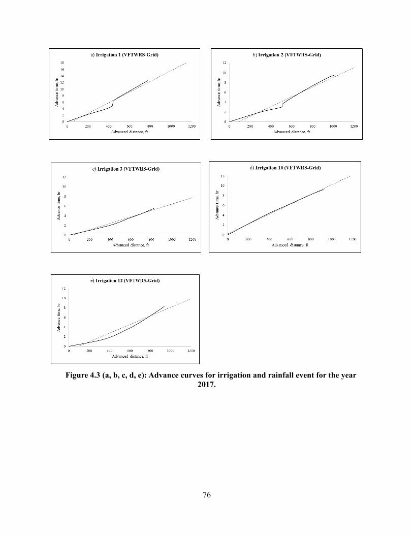
76

Figure 4.3 (a, b, c, d, e): Advance curves for irrigation and rainfall event for the year

2017.

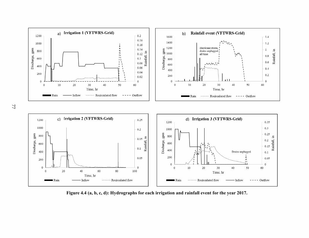
77

Figure 4.4 (a, b, c, d): Hydrographs for each irrigation and rainfall event for the year 2017.

a) b)

c) d)

77

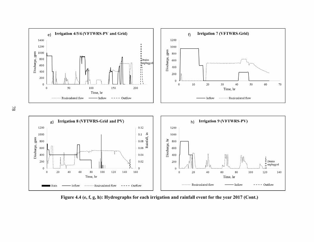
78

Figure 4.4 (e, f, g, h): Hydrographs for each irrigation and rainfall event for the year 2017 (Cont.)

e) f)

g) h)

78

79

Figure 4.4 (i, j, k, l): Hydrographs for each irrigation and rainfall event for the year 2017 (Cont.).

i) j)

k) l)

79

80

Table 4.2: Summary of all the irrigation and rainfall events for the year 2017

Irrigation/

Precipitation Date

Total

hours

Avg total

flow rate

(l/s)

Avg

furrow

flow rate

(l/s)

Water

applied

(ha-cm)

Water

applied

(ha-

cm/ha)

Precipit

ation

(cm)

Runoff

(ha-

cm/ha)

Deep

Percolation

(ha-cm/ha)

Water

recirculate

d (ac-in/ac)

Tail-

water

ratio

Irrigatio

n

efficienc

y (%)

Est. irri.

effi. w/o

VFTWRS

(%)

Rainfall

capture (cm)

VFTWRS G 6/15/2017 49 38.74 0.076 126 4.19 0.00 0.30 N/A 0.00 0.06 93.0 85.4 N/A

Precipitation 6/22/2017 N/A N/A N/A N/A N/A 9.98 4.83 N/A 0.00 0.54 N/A N/A 5.16

VFTWRS G 6/30/2017 54.5 23.47 0.046 68 2.26 0.00 0.00 0.000 1.67 0 100* 73.5 N/A

Precipitation 7/3/2017 N/A N/A N/A N/A N/A 0.43 N/A 0.000 0.04 0 N/A N/A 0.43

VFTWRS G 7/7/2017 48.5 30.28 0.059 63 2.11 1.93 1.09 0.000 2.93 0.27 73.0 54.0 0.84

VFTWR-PV 7/10/2017 74 N/A 0.028 57 1.91 0.00 0.00 0.000 1.36 0 100* 74.3 N/A

VFTWR-PV 7/13/2017 48.5 24.16 0.047 66 2.21 0.00 0.00 0.001 1.26 0 99.961 78.3 N/A

VFTWRS G 7/16/2017 53 58.68 0.115 101 3.35 0.00 0.51 0.036 8.47 0.15 83.8 37.6 N/A

VFTWRS G 7/21/2017 74 N/A 0.078 77 2.64 0.00 0.00 0.127 9.31 0 95.2 35.1 N/A

VFTWRS

G+PV 7/24/2017 149 N/A 0.070 141 4.70 0.74 0.05 0.076 16.75 0.008 97.7 39.1 0.69

VFTWR-PV 7/30/2017 120 11.36 0.022 59 2.03 0.13 0.05 0.025 2.78 0.02 96.5 59.4 0.08

VFTWRS G 8/5/2017 103 32.87 0.064 70 2.41 0.00 0.13 0.025 12.30 0.05 93.7 27.0 N/A

VFTWR-PV 8/11/2017 74 N/A 0.022 33 1.14 1.52 0.57 0.000 1.90 0.21 78.7 58.4 0.96

VFTWRS G 8/19/2017 67 24.35 0.048 59 2.01 0.30 0.08 0.002 4.18 0.04 96.6 51.4 0.23

VFTWR-PV 8/22/2017 188 6.56 0.013 48 1.65 0.00 1.27 N/A 2.88 0.79 23.1 12.5 N/A

VFTWRS G 8/30/2017 N/A N/A N/A N/A N/A 8.31 6.55 N/A 5.71 0.79 N/A N/A 1.75

Total 27.83

(Avg)

0.053

(Avg) 846 33 23 15 0.293

- - - 10

*Irrigation efficiency doesn’t include evaporation losses from the field.

80

81

4.3 Irrigation efficiency discussion (2016-17)

Continuous flow irrigation (CFI): The irrigation efficiency for this system was observed to be

in between 46% and 83%, the tail-water ratio was between 0.17 and 0.53, and the average furrow

flow rate was between 0.08 and 0.10 l/s. The irrigation efficiency started out high earlier in the

season (83%) and it decreased to 46% as the growing season progressed.

Surge irrigation (SI): The irrigation efficiency for this system was measured to be between 32%

and 94%, the tail-water ratio was between 0.04 and 2.77, and the average furrow flow rate was

between 0.08 and 0.10 l/s. Similar to the CFI events, the irrigation efficiency was higher earlier

in the season (94%) and it decreased to 32% towards the end of the growing season.

As the season progressed and soil sealing increased and water demand increased, the irrigation

efficiencies for CFI and SI events decreased. This data suggested that as the growing season

progressed, decrease in irrigation efficiencies caused reduction in water supply to the rice plants

at the time in the season when plant water demand is highest. This corresponded with sensor

trends (Figure A.8) and suggested that monitoring of soil moisture and taking steps to improve

irrigation efficiency later in the season is needed to improve water delivery to furrow irrigated

rice.

VFTWRS-Grid: The irrigation efficiency for both years was between 84% and 99%. The

irrigation efficiency for VFTWRS-Grid remained similar irrespective of the time into the

growing season. The lower range for irrigation efficiencies were due to the result of poor drain

plug installation. It is anticipated that a better management can result in higher irrigation

efficiency. The tail-water ratio was between 0.04 and 0.19 while the average furrow flow rate

82

was between 0.05 to 0.12 l/s. The difference in furrow flow rate was due to the variable flow rate

available at the research centre.

VFTWRS-PV: The irrigation efficiency for these events varied between 78% and 99%. The

irrigation efficiency for some of the VFTWRS-PV events were observed to be higher than

VFTWRS-Grid events. It should be noted that the VFTWRS-PV irrigation events were managed

in a way different than the VFTWRS-Grid events. The irrigation was started at night and was

turned off during the day (water applied for about 12 hr). VFTWRS-PV was continued to be

operated and no additional water from the source was added during this period. A new irrigation

event was started immediately after no more tail-water was available at the bottom of the field.

The drains remained plugged for this duration and therefore no runoff water was observed for the

events which show higher efficiency.

The irrigation efficiency is expected to be low if the irrigation events are managed in a way

similar to VFTWRS-Grid. In VFTWRS-Grid events, volume of irrigation water applied from the

source was approximately twice of what was applied in VFTWRS-Solar events. If the same

volume is applied, then this can result in a high volume of tail-water. The data has suggested that

the volume of water recirculated using solar energy by the VFTWRS is lower in comparison to

that recirculated using grid power in a day. The VFTWRS-PV would be unable to recirculate this

increased volume of tail-water before it would start to overflow. Hence, the overflow from the

drains will cause a decrease in the irrigation efficiency. The efficiency results could also change

if the row crop in the study is different than rice. Row crops like soybean and corn should not be

irrigated for a duration of more than 40 hr, hence, for each irrigation event field would have to be

drained after 40 hr. This could result in runoff water which could in turn decrease irrigation

efficiency.

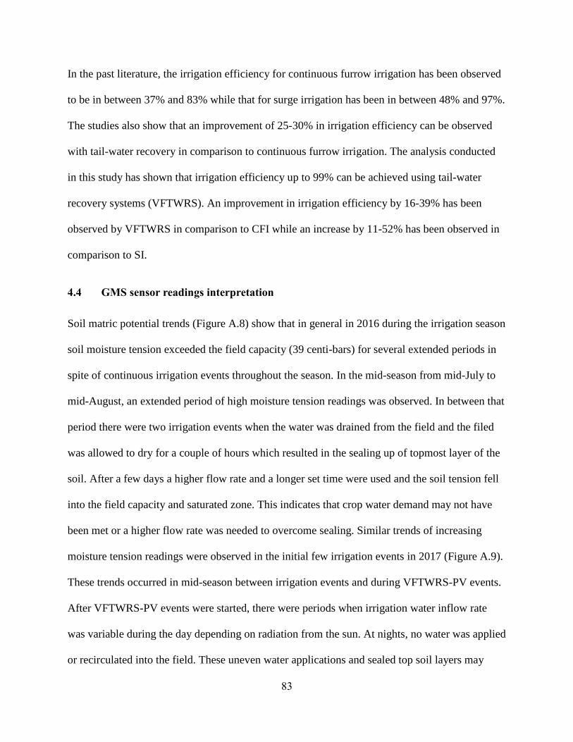
83

In the past literature, the irrigation efficiency for continuous furrow irrigation has been observed

to be in between 37% and 83% while that for surge irrigation has been in between 48% and 97%.

The studies also show that an improvement of 25-30% in irrigation efficiency can be observed

with tail-water recovery in comparison to continuous furrow irrigation. The analysis conducted

in this study has shown that irrigation efficiency up to 99% can be achieved using tail-water

recovery systems (VFTWRS). An improvement in irrigation efficiency by 16-39% has been

observed by VFTWRS in comparison to CFI while an increase by 11-52% has been observed in

comparison to SI.

4.4 GMS sensor readings interpretation

Soil matric potential trends (Figure A.8) show that in general in 2016 during the irrigation season

soil moisture tension exceeded the field capacity (39 centi-bars) for several extended periods in

spite of continuous irrigation events throughout the season. In the mid-season from mid-July to

mid-August, an extended period of high moisture tension readings was observed. In between that

period there were two irrigation events when the water was drained from the field and the filed

was allowed to dry for a couple of hours which resulted in the sealing up of topmost layer of the

soil. After a few days a higher flow rate and a longer set time were used and the soil tension fell

into the field capacity and saturated zone. This indicates that crop water demand may not have

been met or a higher flow rate was needed to overcome sealing. Similar trends of increasing

moisture tension readings were observed in the initial few irrigation events in 2017 (Figure A.9).

These trends occurred in mid-season between irrigation events and during VFTWRS-PV events.

After VFTWRS-PV events were started, there were periods when irrigation water inflow rate

was variable during the day depending on radiation from the sun. At nights, no water was applied

or recirculated into the field. These uneven water applications and sealed top soil layers may

84

have resulted in rising tension readings. While there were high soil tension levels, no visual

stress in the crops was observed. At harvest, in many of the plots, no visual difference in rice

height or color between the row and bed was observed as is typical in furrow rice that has

experienced stress. While often the top of the bed was dry, saturated soil in the beds appeared to

be providing water to the bed and visually one could not detect any visual stress difference

between a bed plants and a furrow plants. We believe these irrigation shortcomings in furrow

irrigation may help explain why furrow irrigated rice does not generate the same yields as

flooded rice. Thus additional work is warranted to overcome these issues in furrow irrigation to

maintain lower soil water thresholds for rice in this production system.

4.5 Solar data analysis

The data from the panels was obtained during the period when PV modules were connected to

the utility. The data from the months March to June, 2017 were used for this analysis. The

relationship between the energy generated from the panels and the solar irradiance was found to

be linear with a goodness of fit (R2) 0.83 (Figure 4.5). The relationship between estimated energy

from the panels and actual energy generated from the panels was also found to be linear with an

R-squared value of 0.83 indicating that the actual power generated from the panels were very

close to the estimated potential energy generated from the panels (Figure 4.6). The energy

generated from panels using solar irradiance data was estimated for the last 10 years for each

month. It was observed that the average monthly solar radiation as well as the energy estimated

from the PV modules between years were comparable to each other between years (Figure 4.7).

The total estimated energy that can be generated from the PV modules for the purpose of net

metering during the months from September to May was 2,240 kWh at the rate of $0.10/unit.

This estimate was obtained from the 10 years daily average data for each month. The PV

85

modules for these nine months were connected to the utility to obtain credit from the utility

provider at the RREC. The payback period for the PV modules is explained in the economic

feasibility section.

Figure 4.5: Data acquired from solar panels from March to June (both panels at 15deg

from the zenith)

Figure 4.6: Relationship between estimated energy and actual energy from the PV

modules

86

Figure 4.7: Estimated Power generation from panels for 10 years, from historical

radiation data

4.6 Pump testing

4.6.1 Pump curve

The discharge and TDH data from 2016 and 2017 were used to develop a system curve (Figure

4.10). The data included in the curve was obtained when the VFTWRS was operated using

power-grid in field experiments. Following linear relationship was obtained between discharge,

Q and TDH, H with an R2 value of 0.35 (Figure 4.9).

Figure 4.8: Relationship between total dynamic head and discharge of VFTWRS during

irrigation (System Curve)

87

Pump curve was obtained from data collected from the pump testing (Figure 4.10). The system

curve data was superimposed with the data obtained from pump testing. The relationship

between TDH and discharge for each frequency was found to be exponential with an R2 value

between 0.97 and 0.99. The highest pump efficiency of 93% was obtained at 50 Hz for a TDH of

about 1.83 m (6 ft) and discharge of about 30 l/s (480 gpm). The highest efficiency of 83% was

calculated at 60 Hz. During the irrigation season, the pump usually operated between 25 and 32

l/s (400 and 500 gpm). The efficiencies for this range of discharge varied from 77 to 93% for

frequencies at 50 and 60 Hz.

Figure 4.9: Pump curve and system curve for the VFTWRS

4.6.2 Nebraska pumping plant performance criteria and pump efficiency

The % of NPPPC was calculated for each irrigation event for both year, 2016 and 2017 (Figure

4.11). During pump operation it was observed that actual discharge from the pump which

resulted in recirculation of tail-water to the top of the field was for pump frequency of 28.5 Hz

and more. Therefore, data for frequency greater than 28.5 Hz was included in % of NPPPC

R² = 0.9761

R² = 0.9947

R² = 0.9702

R² = 0.977

0

2

4

6

8

10

12

14

16

18

0 100 200 300 400 500 600 700

TD

H, ft

Discharge, gpm

35 Hz 40 Hz 50 Hz 60 Linear (system curve)

86%

79%

83%

63%

55%

57%

46%

77%84%

93%

75%

59%

46%

35%

26%

15%

9%

78%

74%

64%

58%36%

21%

11%

87%65%

49%29%

21%

11%

50%

88

calculation. For VFTWRS-Grid operation, pump operation was mostly at frequency of 60 Hz

and the % of NPPPC greater than 90% (and average pump efficiency of 76%) was observed for

frequencies greater than 45 Hz, in general. The mean % of NPPPC for was found to be 98%,

however, for most part of the pump operation the % of NPPPC was between 90 and 120%.

VFTWRS-PV was mostly operated at frequencies between 28.5 and 30 Hz. This is because

cloudy weather was observed for these events resulting in a low energy available for the pump.

The % of NPPPC value was variable throughout the solar powered pump operation and was

anywhere between 30 and 110% while the mean was 77%. The pump efficiency for VFTWRS-

PV was an average of 61%. From the analyzed data it can be concluded that VFTWRS had

higher % of NPPPC when operated using grid energy source as compared to a solar source.

Figure 4.10 (a, b): % of NPPPC distribution with respect to motor frequency for a)

VFTWRS-PV and b) VFTWRS-Grid.

4.7 Rice variety results

4.7.1 Yield

The yields for each rice variety were compared to each other. In 2016 and 2017, there was a

significant interaction effect of variety on yield (P<0.0001). Statistical analyses for 2016 yield data

a) b)

89

were done at 99% confidence level (data was normal at α=0.01) while those in 2017 were done at

95% confidence interval (Table 4.3). Yields for hybrid rice varieties were greater than the

conventional rice varieties in general for both years. In 2016, the best yield of 8,499 kg/ha (168.5

bu/ac) was observed for XL753 and the lowest study yield of 4,882 kg/ha (96.8 bu/ac) was

observed for 1099. Hybrid varieties were not significantly different from each other. Also,

conventional rice varieties were not significantly different from each other. Yields of only two

conventional rice varieties, Jupiter (6,376 kg/ha or 126.4 bu/ac) and Mermentau (5,861 kg/ha or

116.2 bu/ac), were comparable to XL 745. In 2017, rice yields were better than 2016 due to better

irrigation management. Highest average yield of 9,533 kg/ha (189 bu/ac) were produced by

XL753. Average yield from all hybrid rice varieties was calculated as 8,777 kg/ha (174 bu/ac)

while 6,557 kg/ha (130 bu/ac) was calculated for conventional rice varieties. Varieties had a similar

effect on water use efficiencies as they had on crop yield (Table 4.3). It should be noted that the

field was in its second year of continuous rice production in 2017 and the planting date was very

late relative to the area. Thus yields are likely not representative of what farmer would expect to

obtain in a rice-soybean rotation with an earlier planting date. Higher conventional yields would

be expected with an earlier planting date.

90

Table 4.3: Yield differences between variety and water use efficiency differences between

variety revealed by analysis of variance (Tukey honest significant difference method for

mean comparison) for 2016 and 2017

2016 2017

Variety

Yield

[kg/ha (bu/ac)]

(P<0.0001)

WUE

[kg/ha-cm (bu/ac-

in)]

(P<0.0001)

Variety Yield

(kg/ha)/(bu/ac)

(P<0.0001)

WUE

(kg/ha-cm)/(bu/ac-

in)

(P<0.0001)

XL753 8,524 (169) A* 55.5 (5.6) A* XL753 9,533 (189) A 98.7 (9.9) A

XL729 8,323 (165) AB 54.5 (5.5) AB XP4534 8,928 (177) A 92.6 (9.3) A

XP756 8,020 (159) AB 52.5 (5.3) AB Gemini 8,777 (174) A 90.6 (9.1) A

4523 8,020 (159) AB 52.5 (5.3) AB CL7311 8,676 (172) A 90.0 (9.1) A

XL745 7,768 (154) ABC 50.5 (5.1) ABC XP754 7,919 (157) A B 82.1 (8.3) A B

Jupiter 6,355 (126) BCD 41.6 (4.2)

BCD Jupiter 7,162 (142) B 74.1 (7.5) B

Mermenta

-u 5,851 (116) CD 38.6 (3.9)

CD Diamond 6,789 (133) B 69.3 (7.0) B

Diamond 5,447 (108) D 35.7 (3.6)

D CL153 6,254 (124) B 64.8 (6.5) B

Francis 5,246 (104) D 34.7 (3.5)

D CL172 6204 (23) B 64.3 (6.5) B

Titan 4,994 (99) D 32.7 (3.3)

D

1099 4,893 (97) D 31.7 (3.2)

D

*Means within a column followed by different letters

are significantly different at α = 0.01 level.

*Means within a column followed by different letters

are significantly different at α = 0.05 level.

4.7.2 Plant height

In both years, plant heights were not influenced by their position on bed or furrow; however,

their position along the furrow length (Top/Middle/Bottom, where Top is top 1/3rd furrow length,

Middle is middle 1/3rd furrow length and Bottom is bottom 1/3rd furrow length) had significant

effect on plant heights. In 2016, plants at bottom were the tallest followed by those at middle and

top positions, respectively (alpha = 0.05) (Table 4.4). Plant heights were also analyzed to study

differences within varieties (Table 4.4). Four out of eleven rice variety’s plant heights were

influenced by their positions along the furrow length where plants at the bottom position were

taller than the rest (Table 4.4). In the year 2017, plants at bottom were still the tallest, however,

91

no significant differences were seen between the plant heights at the middle and top positions.

For plant height differences within varieties, eight out of the nine rice varieties were influenced

by their position along the furrow length. Plants at the top were always the shortest (Table 4.5).

No differences in plant height in furrow and bed within the varieties blocked by position along

the furrow length for both years. No effect of plant position at beds and furrows were detected on

plant heights when interaction was blocked by variety.

92

Table 4.4: Plant height differences by position within variety revealed by analysis of

variance (Tukey honest significant difference method for mean comparison)

Plant heights (m)/(ft)

Position Bottom Middle Top

2016

XL729 (P=0.0006) 42.0/4.2 A* 37.5/3.8 B* 39.1/4.0 B*

XL745 (P=0.0135) 40.2/4.1 A 38.2/3.9 B 38.7/3.9 AB

XP756 (P=0.0325) 38.7/3.9 A 36.3/3.7 B 38.3/3.9 AB

XL753 (P=0.0674) 39.4/4.0 A 35.9/3.6 A 37.1/3.7 A

Francis (0.2040) 34.6/3.5 A 32.9/3.3 A 33.1/3.3 A

1099 (P=0.6415) 33.7/3.4 A 33.4/3.4 A 33.1/3.3 A

Diamond (P=0.0102) 34.1/3.4 A 31.2/3.2 B 33.2/3.4 AB

4523 (P=0.2210) 32.6/3.3 A 30.8/3.1 A 32.8/3.3 A

Mermentau(P=0.3115) 32.6/3.3 A 31.8/3.2 A 31.5/3.2 A

Jupiter (P=0.1038) 30.8/3.1 A 30.1/3.0 A 28.5/2.9 A

Titan (P=0.2273) 28.3/2.9 A 28.4/2.9 A 29.1/2.9 A

2017

CL153 (P=0.0012) 31.4/3.2 A* 29.3/3.0 B* 27.5/2.8 B*

CL172 (P=0.1262) 28.2/2.9 A 26.6/2.7 A 26.4/2.7 A

CL7311 (P=0.0066) 37.9/3.8 A 34.6/3.5 B 35.1/3.5 B

Diamond (P=0.0463) 33.6/3.4 A 33.6/3.4 A 31.4/3.2 B

Gemini (0.0014) 40.6/4.1 A 36.3/3.7 B 37.2/3.8 B

Jupiter (P=0.0173) 30.2/3.1 A 30.0/3.0 A 28.7/2.9 B

XL753 (P=0.0007) 37.6/3.8 A 34.5/3.5 B 34.4/3.5 B

XP4534 (P<0.0001) 32.4/3.3 A 28.4/2.9 B 27.9/2.8 B

XP754 (P=0.0257) 36.4/3.7 A 32.9/3.3 B 31.6/3.2 B

*Means within a column followed by different letters are significantly different

at α = 0.05 level.

93

Table 4.5: Plant height differences between positions along furrow length revealed by

analysis of variance blocked by Variety (Tukey honest significant difference method for

mean comparison)

Plant position along

furrow length

2016 2017

Plant Height (m)/(ft.)

(P<0.0001) (P<0.0001)

Bottom 1.08/3.55 A* 1.05/3.46 A*

Top 1.05/3.44 B 0.96/3.14 B

Middle 1.02/3.36 C 0.98/3.21 B

*Means within a column followed by different letters are significantly

different at α = 0.05 level.

4.7.3 Growth stage obervations

In 2016, growth stage observations were taken on 18th August. It was observed that all of the hybrid

rice varieties were 100% headed and were anywhere in between R6 to R9 stage. Most of the

conventional rice varieties were not completely headed and were anywhere in between R4 to R6

(milk) (Table 4.6). In 2017, growth stage observations notes were taken on 12th August. It was

observed that different replications were headed in different percentages depending upon the

presence of weed (Barnyard grass) in the plots. In general, most of the hybrid variety plots were

headed anywhere between 60-90% and conventional variety plots were headed between 0-60%

(Table 4.7).

94

Table 4.6: Growth stage observations taken on 18th August 2016 for all rice plots (similar

for all replications within varieties)

Variety % headed Heading Stage

XL 729 100% R6 Stage (milk to soft dough)

XL 753 100% R6 Stage (milk to soft dough)

1099 100% R6 Stage (milk to soft dough)

XL 745 100% R6 (milk)

XP 756 50% R4 to R5

4523 100% R8 to R9

Diamond 90% R5

Jupiter 80% R5

Mermentau 100% R5 to R6 (milk)

Titan 90% R6 (milk)

Francis 100% R6 (milk)

Table 4.7: Heading notes taken on 12th August 2017 for all rice plots

Variety % Headed Heading Stage

Rep 1 Rep 2 Rep 3 Rep 1 Rep 2 Rep 3

XP754 20% 5% 0-5% R5 R2 R2

CL7311 80% 60% 10-20% (grassy) R6 R5-R6 R4

CL172 30% 30-40% (grassy) 40% (grassy) R4-R5 R4 R5

Jupiter 10% 0% (grassy) 2% R4 R3-R4 R3

CL153 60-70% 60% 50% R5 R5 R5

XP4534 70% 75% 70% R5-R6 R6-R7 R6-R7

XL753 80-90% 85% 70-80% R5 R6 R6

Diamond 5-10% 10% 5% R4 R4 R3-R4

Gemini 30% 40% 10-20 R5 R6 R4

4.8 Economic feasibility results

The water budgeting summary for all of the scenarios are shown in the Table 4.8. The total

irrigation requirement for each scenarios was obtained from this table and was included in the

row-rice budget 2017 to estimate operating expenses and revenue.

95

Table 4.8: Water budget summary for each scenarios for the year 2016 and 2017 as

observed in field experiments

Note: For the economic analysis, water budgeting for VFTWRS-PV was adjusted to best

represent the system and was managed differently than the VFTWRS-Grid. VFTWRS was

allowed to be operated each day and was never turned off. The only events which resulted in

runoff were caused by the overflow during heavy rainfall events. Therefore, overall irrigation

efficiency for solar events was 96% and higher than VFTWRS-Grid. If the VFTWRS-PV events

are directly compared to the VFTWRS-Grid events, the irrigation efficiencies thus obtained are

expected to be less than that for VFTWRS-Grid. The reason would be less and variable power

availability from the PV modules for VFTWRS-PV events.

Date

Recd. tail-

water (ha-

cm/ha)

Irri. water,

(ha-cm/ha)

Overflow

(ha-cm/ha)

Pptn.

(cm)

Overall irri.

efficiency

(%)

Evap. from

pit

(ha-cm/ha)

Deep

percolation

(ha-cm/ha)

2016

VFTWRS-Grid 35.05 47.80 6.25 14.17 89 ~0 0.30

VFTWRS-Solar 15.24 27.94 2.26 14.17 96.7 ~0 0.30

TWR-FPit 40.64 38.10 1.78 14.17 94.5 1.52 0.30

TWR-HPit 50.80 30.48 8.38 14.17 88.56 0.86 0.30

2017

VFTWRS-Grid 38.10 27.94 16.70 24.41 93 ~0 0.28

VFTWRS-Solar 12.70 20.83 4.32 24.41 96.2 ~0 0.28

TWR-FPit 35.56 31.75 1.63 24.41 94.6 1.40 0.28

TWR-HPit 33.02 35.56 4.57 24.41 96.56 0.81 0.28

Overall Average for 2016 and 2017

VFTWRS-Grid 36.58 37.87 11.47 19.29 91 ~0 0.29

VFTWRS-Solar 13.97 24.38 3.29 19.29 96.45 ~0 0.29

TWR-FPit 38.10 34.93 1.70 19.29 94.55 1.46 0.29

TWR-HPit 41.91 33.02 6.48 19.29 92.3 0.84 0.29

96

Table 4.9: Net returns, revenue and other costs associated with each scenario

Tail-water recovery

system

Power

Source

Distance

from power

source (m)

Pipeline Type

Net returns ($/ha) Revenue

* ($/ha)

Fixed

capital costs

**($/ha)

Opportu

nity cost

($/ha)

Monetar

y benefit

($/ha)

Surface

water

source

Ground

-water

source

(4) VFTWRS Grid 61 Lay-flat $576 $548 $2,312 $965 $0 $0

(5) VFTWRS Grid 61 Underground $605 $578 $2,312 $1,634 $0 $0

(6) VFTWRS Solar N/A Lay-flat $568 $522 $2,312 $1,384 $0 $15

(7) VFTWRS Solar N/A Underground $598 $551 $2,312 $2,026 $0 $15

(8) TWR-full pit Grid 61 Underground $588 $557 $2,312 $3,933 $41 $0

(9) TWR-half pit Grid 61 Underground $586 $550 $2,312 $3,066 $20 $0

(10) TWR-full pit Diesel 61 Underground $556 $525 $2,312 $3,847 $39 $0

(11) TWR-half pit Diesel N/A Underground $564 $527 $2,312 $2,983 $19 $0

(1) VFTWRS Grid 150 Lay-flat $576 $548 $2,312 $985 $0 $0




(1) VFTWRS Grid 300 Lay-flat $576 $548 $2,312 $1,020 $0 $0








* obtained from Crop Budget 2017 developed at the Rice Research and Extension Center, Stuttgart AR for row rice

** calculated from the retail cost of each equipment, raw material and labor involved in each scenario

96

97

Table 4.9: Net returns, revenue and other costs associated with each scenario (Cont.)

Tail-water recovery

system

Power

Source

Distance

from power

source (m)

Pipeline Type

Net returns ($/ha) Revenue

* ($/ha)

Fixed

capital costs

**($/ha)

Opportu

nity cost

($/ha)

Monetar

y benefit

($/ha)

Surface

water

source

Ground

-water

source













(1) VFTWRS Grid 1,050 Lay-flat $576 $548 $2,312 $1,351 $0 $0

(2) VFTWRS Grid 1,050 Underground $605 $578 $2,312 $2,020 $0 $0

(5) TWR-full pit Grid 1,050 Underground $588 $557 $2,312 $4,345 $41 $0

(6) TW-half pit Grid 1,050 Underground $586 $550 $2,312 $3,465 $20 $0

(1) VFTWRS Grid 1,200 Lay-flat $576 $548 $2,312 $1,408 $0 $0

(2) VFTWRS Grid 1,200 Underground $605 $578 $2,312 $2,078 $0 $0

(5) TWR-full pit Grid 1,200 Underground $588 $557 $2,312 $4,406 $41 $0

(6) TWR-half pit Grid 1,200 Underground $586 $550 $2,312 $3,524 $20 $0

* obtained from Crop Budget 2017 developed at the Rice Research and Extension Center, Stuttgart AR for row rice

** calculated from the retail cost of each equipment, raw material and labor involved in each scenario

97

98

Table 4.10: Net present value (NPV) at 4% interest rate and discounted payback period (DPP) for each scenario (in year) at

4% discount rate for surface water and groundwater source

Tail-water recovery

system

Power

Source

Distance

from power

source (m)

Pipeline Type NPV ($/ha) DPP (years) NPV ($/ha) DPP (years)

Surface water Groundwater

(1) VFTWRS Grid 61 Lay-flat $8,031 1.77 $7,598 1.86

(2) VFTWRS Grid 61 Underground $7,821 2.92 $7,391 3.06

(3) VFTWRS Solar N/A Lay-flat $7,725 2.55 $7,003 2.78

(4) VFTWRS Solar N/A Underground $7,542 3.62 $6,823 3.9

(5) TWR-full pit Grid 61 Underground $4,618 8.64 $4,166 9.08

(6) TWR-half pit Grid 61 Underground $5,780 6.23 $5,241 6.66

(7) TWR-full pit Diesel 61 Underground $4,243 8.99 $3,791 9.32

(8) TWR-half pit Diesel N/A Underground $5,525 6.31 $4,972 6.78














98

99

Table 4.10: Net present value (NPV) at 4% interest rate and discounted payback period (DPP) for each scenario (in year) at

4% discount rate for surface water and groundwater source (Cont.)

Tail-water recovery

system

Power

Source

Distance

from power

source (m)

Pipeline Type NPV ($/ha) DPP (years) NPV ($/ha) DPP (years)

Surface water Groundwater












(1) VFTWRS Grid 1,050 Lay-flat $7,643 2.5 $7,213 2.65

(2) VFTWRS Grid 1,050 Underground $7,435 3.64 $7,003 3.85

(5) TWR-full pit Grid 1,050 Underground $4,206 9.72 $3,754 10.42

(6) TW-half pit Grid 1,050 Underground $5,382 7.14 $4,841 7.7

(1) VFTWRS Grid 1,200 Lay-flat $7,586 2.39 $7,156 2.77

(2) VFTWRS Grid 1,200 Underground $7,379 3.53 $6,946 3.96

(5) TWR-full pit Grid 1,200 Underground $4,146 9.55 $3,692 10.6

(6) TWR-half pit Grid 1,200 Underground $5,323 6.99 $4,784 7.86

99

100

The initial investment and annual operating cost for each scenario is represented in the Table 4.9.

The monetary benefit and opportunity costs are also depicted in the table, as applicable. Net

present value (NPV) and discounted payback period (DPP) used in this section is for a discount

rate of 4% (Table 4.10). NPV and DPP was also calculated for discount rates of 5%, 6%, 7%, 8%

and 9% which are presented in the Tables A.9, A.10, A.11, A.12 and A.13. Water budgeting and

economic analysis results are discussed within the sections explained below while water budget

summary is provided in Table 4.8.

4.8.1 Scenario 1 and 1-x foot: VFTWRS with lay-flat pipe at different distances from

power source

The total irrigation water requirement observed for all of these scenarios was 15 ac-in/ac.

Scenario 1 (61 m) had the highest NPV of $8,01 and the least SPP of almost 1.5 years while

lowest NPV of $7,586 and a SPP of 2.3 years was calculated for Scenario 1- 1,200 m from the

supply source. As the distance from the electric supply increased, the capital cost of the system

increased by 2.3% for 150 m (500 ft), 6% for 300 m (1,000 ft), 10% for 450 m (1,500 ft), 13.8%

for 600 m (2,000 ft), 22.5% for 750 m (2,500 ft), 27% for 900 m (3,000 ft), 43% for 1,050 m

(3,500 ft) and 50% for 1,200 m (4,000 ft). The NPV of the system was observed to decrease and

the discounted payback period increased as the distance increased from 61 m (200 ft) to 1,200 m

(4,000 ft) (Table 4.10).

4.8.2 Scenario 2 and 2-x foot: VFTWRS with underground irrigation pipeline at different

distances from power source

The installation of irrigation pipeline alone cost almost $10,000. This increased the total

installation cost of the system by 46% in comparison to Scenario 1. The base scenario for this

category was Scenario 2 (61 m) with the highest NPV $7,821 and a SPP of 2.92 years. Lowest

NPV of $7,621 was calculated for Scenario 2 at 1,200 m. The increase in capital cost of the

101

scenarios from the base scenario as the distance increased was by 1.35% for 150 m, 3.5% for 300

m, 5.7% for 450 m, 8% for 600m, 12.9% for 750 m, 15.6% for 900m, 24.7% for 1,050 m and

28.3% for 1,200 m. The NPV of the scenario sin this category also decreased and DPP increased

as the distance increased (Table 4.10).

4.8.3 Scenario 3: VFTWRS with lay-flat pipeline using solar panels

A total of 2,204 kWh of energy was estimated to be generated for off season months. Water

balance data showed that total irrigation requirement was about 14 ha-cm/ha for this system. The

total irrigation efficiency for this system was 96%. The difference in management of irrigation

events resulted in a change in irrigation efficiency in comparison to Scenarios 1 and 2. The water

balance for this scenario is provided in Tables A.2 and A.6. The total cost of inverter, solar

panels and their structure was about $7,000. The increase in the capital cost of this system

comparison to that of Scenario 1 was by 37%.This value was used to estimate monetary benefit

of $14.95/ha ($6.05/ac). The capital cost of this system was 54% higher than that of base

Scenario 1. The NPV of this scenario was $7,725 and a DPP of 2.55 years.

4.8.4 Scenario 4: VFTWRS with underground pipeline using solar panels

The water balance for this scenario is provided in Tables A.2 and A.6. The additional cost for

solar panel structure was about $17,000. The capital cost of this system was 126% higher than

that of base Scenario 1. The NPV of this scenario was $7,542 and a DPP of 3.62 years.

4.8.5 Scenarios 5, 7 and 5-x foot: Tail-water recovery full width (electric/diesel pump)

In 2016, a total irrigation water of 41 ha-cm/ha (16 ac-in/ac) was supplied from a near-by surface

water source while 38 ha-cm/ha (15 ac-in/ac) of irrigation water was supplied from tail-water

which was collected in the ditch. A total of 12.7 cm (5 in) of rainfall was captured from a total

precipitation of 14 cm (5.5 in) in 2016. Average irrigation efficiency was calculated as 91%. By

102

the end of the irrigation season 50 ha-cm (24.3 ac-in) of tail-water was remaining in the TWR

ditch. A total overflow of 27 ha-cm (13.1 ac-in/ac) occurred during the season. Rainfall events

documented in the water balance tables are those which resulted in runoff water. The other

rainfall events were excluded (Tables A.4). In 2017, a total irrigation water of 163 ha-cm/ha

(64.2 ac-in/ac) was supplied from a near-by surface water source while 177 ha-cm/ha (70 ac-

in/ac) of irrigation water was supplied from tail-water which was collected in the ditch. Total

rainfall capture was 23 cm (9 in) from a total rainfall of 25.4 cm (10 in). Average irrigation

efficiency was 90%. By the end of the irrigation season 106 ha-cm (51.46 ac-in) of tail-water

was remaining in the TWR ditch. A total overflow of 45 ha-cm (21.8 ac-in) occurred during the

season (Table A.5). Average overall irrigation efficiency for both years was 94.5%. Scenario 7 is

the same as Scenario 5 except that the tail-water recovery pump was a diesel operated pump

rather than an electric pump.

The highest NPV in this category was $4,618 for the base scenario 5 (61 m) with a DPP of 8.64

years. The NPV for scenario 7 (diesel TWR pump) was $4,243 with a DPP of 9 years. The

capital cost of scenarios 5 and 7 was 330% and 328% greater than base scenario 1. The increase

in capital cost in comparison to base scenario 5 was by 0.6% for 150 m, 1.5% for 300 m, 2.5%

for 450 m, 3.4% for 600 m, 5.6% for 750 m, 6.8% for 900 m, 10.7% for 1,050 m and 12.3% for

1,200 m.

4.8.6 Scenarios 6, 8 and 6-x foot: Tail-water recovery half width (electric/diesel pump)

In 2016, a total irrigation water of 50 ha-cm/ha (19.7 ac-in/ac) was supplied from a near-by

surface water source while 25.4 ha-cm/ha (10 ac-in/ac) of irrigation water was supplied from

tail-water which was collected in the ditch using an electric tail-water pump. A total of 13 cm

(5.1 in) of rainfall was captured from a total precipitation of 14 cm (5.5 in) in 2016. Average

103

irrigation efficiency was calculated as 88%. By the end of the irrigation season 45 ha-cm (21.84

ac-in) of tail-water was remaining in the TWR ditch. A total overflow of 136 ha-cm (66.02 ac-in)

occurred during the irrigation season (Table A.4). In 2017, a total irrigation water of 33 ha-cm/ha

(13 ac-in/ac) was supplied from a near-by surface water source while 30 ha-cm/ha (11.8 ac-in/ac)

of irrigation water was supplied from tail-water which was collected in the ditch. Total rainfall

capture was 23 cm (9.06 in) from a total rainfall of 25 cm (9.84 in). Average irrigation efficiency

was 96%. By the end of the irrigation season 68 ha-cm/ha (26.78 ac-in/ac) of tail-water was

remaining in the TWR ditch. A total overflow of 133.2 ha-cm (5.4 ac-ft) occurred during the

irrigation season. Average irrigation efficiency for both years was 92.3%. Scenario 8

corresponds to Scenario 6 except the tail-water pump is a diesel operated pump. The highest

NPV in this category was $5,780 for the base scenario 6 (61 m) with a DPP of 6 years. The NPV

for scenario 8 (diesel TWR pump) was $5,525 with a DPP of 6.3 years. The capital cost of

scenarios 6 and 8 was 234% and 232% greater than base scenario 1. The increase in capital cost

in comparison to base scenario 6 was by 0.66% for 150 m, 1.9% for 300 m, 3% for 450 m, 4.2%

for 600 m, 6.9% for 750 m, 8.4% for 900 m, 13.3% for 1,050 m and 15.3% for 1,200 m.

4.8.7 Overall conclusion for all scenarios

From the analysis it was observed that the developed variable flow tail-water recovery system

(VFTWRS) was more feasible than conventional tail-water recovery systems. The highest NPV

of $8,031 (least DPP ~2 years) was observed for Scenario 1 which was the VFTWRS at a

distance of 61 m from the electric power source. It was observed that as this distance increased,

NPV for the scenarios started to decrease. At the distance from the power source greater than

900 m, solar powered VFTWRS had the highest NPV (Scenario 3). Depending on the distance of

farm from the power supply line, the most feasible option will change. The table 4.10 can be

104

used as a guide to identify the best feasible scenario. Least NPV of $4,146 was observed for

Scenario 5-1,200 m which was the scenario of a conventional tail-water recovery system with a

pit along the full width of the field at a distance of 1,200 m from an electric source and a highest

DPP of ~10years.

105

5. Conclusions

A Variable Flow Tail-Water Recovery System (VFTWRS) was evaluated in this study on a

furrow irrigated rice field in Stuttgart, AR. A total of three different irrigation systems were

analyzed in the rice field. These systems were Continuous Furrow Irrigation (CFI), Surge

Irrigation and VFTWRS (on grid and solar panels). Irrigation efficiencies in the literature were

observed to be from 45% to 83% for continuous flow furrow irrigation and from 48% to 97% for

surge irrigation. An improvement by 15%-30% was reported for tail-water recovery irrigation

systems in comparison to continuous flow furrow irrigation method. Average irrigation

efficiency for continuous flow furrow irrigation in the study was 67%, for surge irrigation it was

69% for surge irrigation, for VFTWRS on grid it was 94% and for VFTWRS on solar panels it

was 79%. Improvement in irrigation efficiency for the VFTWRS-Grid was by 16%-39% in

comparison to CFI. It was observed that as the irrigation season progressed, the irrigation

efficiencies for surge irrigation and continuous furrow irrigation decreased. A possible

explanation for such a trend was the sealing up of top soil which was observed as the season

progressed. This could be a reason for a decrease in infiltration and generation of more runoff

water, thus, causing a decrease in the irrigation efficiency. This observation was also validated

by the Granular Matrix Sensor trends.

The VFTWRS was evaluated using the Nebraska Pumping Plant Performance Criteria (NPPPC)

for electric energy. The variables like electric energy consumption, sump water depth, discharge

pressure, motor frequency, and discharge for the VFTWRS were collected using a data logger.

These values were used to determine the percentage of NPPPC for the system. It was observed

that during VFTWRS operation on grid, the system mostly operated at a frequency of 60 Hz.

However, VFTWRS on solar panels was unable to run on its full potential due to cloudy weather

106

conditions. Most of the data obtained for VFTWRS on solar panels were below 30 Hz. The

percentage of NPPPC for VFTWRS on grid had an average value of 98% while that for

VFTWRS on solar panels was 77%. However, it is important to note that the VFTWRS-Grid was

mostly operable at a frequency of more than 45 Hz. The % of NPPPC for frequencies greater

than 45 Hz varied between 90% and 120% (with an average % of NPPPC of 101%). The average

pump efficiency for VFTWRS-Grid was 76% and that for VFTWRS-PV was 61%.

The economic feasibility analysis for VFTWRS was conducted using the Net Present Value

(NPV) and Discounted Payback Period (DPP) methods. The feasibility analysis was conducted

based on the following factors: the size of tail-water recovery pits; distance of tail-water recovery

pump from utility infrastructure; use of PV modules as the power source; use of lay-flat pipes

versus permanent underground irrigation pipeline as the means of water conveyance for tail-

water recirculation. From the analysis it was observed that the VFTWRS-Grid (lay-flat pipe) was

the most feasible system with the highest NPV of $8,031 per ha and with a DPP of 2 years. For

distance up to 900 m (3,000 ft) from the electric power source, VFTWRS system with layflat

pipeline was the most feasible system. When the distance from the utility infrastructure exceeded

900 m (3,000 ft), solar powered VFTWRS with lay-flat pipe was found to be the most feasible.

NPVs of solar powered systems were $7,725 and $7,542 with a DPP of 2.5 and 3.6 years,

respectively. NPVs for conventional tail-water recovery systems with pit were found to be in

between $4,206 and $5,760 while the DPPs were between 6 and 10 years. In general, all of the

designs of tail-water recovery systems with pits had lower NPVs and higher DPPs in comparison

to VFTWRS operated using grid as well as PV modules. Thus, VFTWRS-Grid and PV were

more economically feasible compared to pit based tail-water recovery systems.

107

The yield and plant height analysis for the rice crop in the study was also analyzed. A total of

eleven and ten rice varieties were analyzed for the years 2016 and 2017, respectively. The yield

for hybrid rice varieties was generally higher than the yield for conventional rice varieties for

both years. The rice variety, XL753 had the highest yield for both years (8,524 kg/ha in 2016 and

9,533 kh/ha in 2017) while the highest yield in conventional rice varieties was obtained from

Jupiter (6,355 kg/ha in 2016 and 7,162 kg/ha in 2017). Plant heights were not influenced by their

position on the bed or in the furrow; however, their position along the furrow length

(Top/Middle/Bottom, where Top is the top one-third furrow length, Middle is the middle one-

third furrow length and Bottom is the bottom one-third furrow length) had a significant effect on

plant heights. Plants at the bottom were the tallest; however, no significant differences between

plant heights at bottom and middle were seen in the year 2017. In 2016, plants at top position

were taller than the plants at the middle position. Changes in plant heights could be an indication

of changes in plant yield along the furrow length; however, no statistical analyses on yield at

position along the furrow length were done for the study.

Overall, we were able to evaluate the performance of the VFTWRS in a furrow irrigated field.

The performance parameters included the percentage of NPPPC, irrigation efficiency, NPV and

DPP for the system. Different irrigation systems were also evaluated to provide a comparison

between these systems and the VFTWRS.

108

6. Recommendations

Rice yield in the economic analysis for all of the scenarios was assumed to be the same.

However, the actual yield can be different for VFTWRS-Grid, TWR and VFTWRS-PV

scenarios. Experimental studies can be performed in separate fields for VFTWRS-Grid,

VFTWRS-PV and pit based TWR to collect yield data for each case.

Most of the irrigation events in the study were completed within 40-45 hr from the start

of an irrigation event to simulate irrigation for row crops. However, VFTWRS field

experiments are recommended on row crops to calculate actual irrigation efficiency for

crops like soybean and corn.

The drying periods in between irrigation events resulted in sealing of the top layer of soil

which created large volumes of runoff water. In order to avoid this, it is recommended to

operate VFTWRS continuously without any interruptions each day after the start of first

irrigation. It is suggested to drain fields only before harvest.

In order to improve understanding on the economic feasibility of the VFTWRS, further

case studies are needed. Analyses on soybean-rice rotation, corn, soybean as well as on

different field sizes should be considered.

109

7. References

Allen, R. R., & Musick, J. T. (1994). Graded furrow irrigation of winter wheat with blocked ends.

Applied Engineering in Agriculture, 10(5), 687-692.

Allen, R. R., & Musick, J. T. (2001). Deep ripping and blocked furrow effects on lower 1/3 furrow

irrigation infiltration. Applied Engineering in Agriculture, 17(1), 41.

Arnold, C.A. (Tony) (2009). Water Privatization Trends in the United States: Human Rights, Natio

nal Security and Public Stewardship. William andMary Environmental Law and Policy Review

33: 785.

Arnold, C.A., Norton, C. & Wallen, D. (2009) A Handbook on Land Use and Water for Kentucky

Communities. Kentucky Wet Growth Handbook. Louisville: University of Louisville.

Bali, Khaled. M. (2008, April 19) Cutback irrigation reduces runoff. Western Farm Press.

Retrieved from http://westernfarmpress.com/cutback-irrigation-reduces-runoff on 6-12-2016

Barry, P.J., Hopkin, J. A. & Baker, C. B. (1983). Financial management in agriculture. 4th Edition.

The Interstate Printers and Publishers, Inc., Danville, IL

Bernuth, R. D. (2015). Pumps and pumping systems. Fairfax, VA: Irrigation Association.

Bondurant, J. A., & Willardson, L. S. (1966). Recirculating farm irrigation systems. Irrigation and

Drainage Specialty Conference Proceeding. pp. 243-256.

Bondurant, J. A. (1969). Design of recirculating irrigation systems. Transactions of the American

Society of Agricultural Engineers, 12(2), 195-0198.

Bouldin, J.L., Bickford, N.A., Stroud, H.B. & Guha, G.S. (2004). Tailwater recovery systems for

irrigation: Benefit/cost analysis and water resource conservation technique in Northeast

Arkansas. Journal of the Arkansas Academy of Science, 58.

Broner. (2003) Tailwater recovery for surface irrigation. Fact Sheets: Colorado State University

Cooperative Extension (4.709). Retrieved from

http://irrigationtoolbox.com/ReferenceDocuments/BasicWaterManagement/f56_tailwater_recov

ery_system.pdf on 5-4-2016

Brouwer, C., Goffeau, A., & Heibloem, M. (1985). Irrigation water management: Training manual

No. 1-Introduction to irrigation. Food Agricultural Organization, Rome, Italy.

110

Burt, C. M., Clemmens, A. J., Strelkoff, T. S., Solomon, K. H., Bliesner, R. D., Hardy, L. A., &

Eisenhauer, D. E. (1997). Irrigation performance measures: efficiency and uniformity. Journal of

Irrigation and Drainage Engineering, 123(6), 423-442.

Cahoon, J. E., Mandel, P., & Eisenhauer, D. E. (1995). Management recommendations for sloping

blocked-end furrow irrigation. Applied Engineering in Agriculture, 11(4), 527-533.

Campana, P. E. (2015). PV water pumping systems for agricultural applications. PhD diss.

Sweden: Mälardalen University.

Carman, D. (ND). Tailwater recovery. Phosphorus Best Management Practices. Protecting Water

Quality. Retrieved from http://www.cost869.alterra.nl/SERA17_BMP/BMP_tailwater.pdf on 6-

15-2016.

Clark, B. R., & Hart, R. M. (October 20, 2009). The Mississippi Embayment Regional Aquifer

Study (MERAS): Documentation of a groundwater-flow model constructed to assess water

availability in the Mississippi Embayment (No. 2009-5172). US Geological Survey. Retrieved

from http://pubs.usgs.gov/sir/2009/5172/ on 6-12-2016

Czarnecki, J.M. (May 14, 2014). Conservation practices benefit water quality, wildlife. Mississippi

State University Extension Service. Retrieved from http://extension.msstate.edu/news/extension-

outdoors/2014/conservation-practices-benefit-water-quality-wildlife

Davila, F. M., Capetillo, C. F. B., Fernandez, E. V., & Valdez, J. G. O. (2012). Chapter 1:

Comparing water performance by two different surface irrigation methods. Croatia: InTech

Open Access Publisher.

Delta Plastics® (2016). Pipe Planner. Web-based application. Available at

https://www.pipeplanner.com/

Eisenhauer, D. E., Fekersillassie, D., & Boldt, A. (2000). Feedback-controlled surge irrigation: III.

Field experiments. Transactions of the American Society of Agricultural Engineers, 43(6), 1643.

El-Dine, T. G., & Hosny, M. M. (2000). Field evaluation of surge and continuous flows in furrow

irrigation systems. Water resources management, 14(2), 77-87.

Evans, R. G. (1977). Improved semi-automatic gates for cut-back surface irrigation systems.

Transactions of the American Society of Agricultural Engineers, 20(1), 105-0108.

Falconer, L., Lewis, A., & Krutz, J. (2015). Economic feasibility analysis of tail-water recovery

systems in the Mississippi delta. Southern Agricultural Economics Association Annual Meeting,

January 31-February 3, 2015, Atlanta, Georgia (No. 196721).

111

FAO-UN (2002). World agriculture towards 2015/2030: Summary report. Food and Agriculture

Organization of the United Nations, Rome.

FAO-UN (2015). Food and Agriculture Organization Statistical Pocketbook World Food and

Agriculture. Rome: Food Agricultural Organization of the United Nations.

Foster, R. & Cola, A. (2014). Solar water pumping advances and comparative economics. Energy

Procedia, 57, 1431-1436.

Fritscher, J. (Nov, 15, 2012). NRCS conservation efforts benefit the environment, boosts economy

in Miss. delta town. NRCS Mississippi in Conservation. Available at

https://www.usda.gov/media/blog/2012/11/15/nrcs-conservation-efforts-benefit-environment-

boosts-economy-miss-delta-town (accessed on 12 February 2018).

Gailly, B. (2011). Developing innovative organizations: a roadmap to boost your innovation

potential. Houndmills, Basingstoke, Hampshire: Palgrave Macmillan.

Gaspar, J., Henry, C. G., Duren, M. W., Horton, A. P. & James, H. (2016). Effects of three different

alternate wetting and drying regimes in rice cultivation on yield, water use, and water use

efficiency in a clay soil during a wet year. B. R. Wells Rice Research Studies 2015. 634, 251-

260.

Gopal, C., Mohanraj, M., Chandramohan, P. & Chandrasekar, P. (2013). Renewable energy source

water pumping systems—a literature review. Renewable and Sustainable Energy Reviews, 25,

351-370.

Hagen, L. J., & Sharif, M. (1981). Wind-powered irrigation tailwater system: Sizing the wind

turbine and storage pit. Transactions of the American Society of Agricultural Engineers, 24(1),

103-0106.

Hatiye, S. D., Hari Prasad, K. S., Ojha, C. S. P. & Adeloye, A. J. (2016). Estimation and

characterization of deep percolation from rice and berseem fields using lysimeter experiments

on sandy loam soil. Journal of Hydrologic Engineering, 21(5).

Henry, C. G., Watkins, K. B., Mane, R. U. & Stark, G. L. (2016). Vertical hollow shaft motors for

irrigation: Does premium efficiency payback? American Society of Agricultural Engineers

Annual International Meeting, Orlando- FL.

Hitaj C. & Suttles S. (2016). Trends in U.S. Agriculture’s consumption and production of energy:

Renewable power, shale energy, and cellulosic biomass. (No. 159). U.S. Department of

Agriculture, Economic Research Service.

112

Hofstrand, D. (August 2013). Capital budgeting basics (File C5-240). Ag Decision Maker.

Cooperative Extension Service. Iowa State University of Science and Technology, Ames, Iowa.

Horst, M. G., Shamutalov, S. S., Goncalves, J. M., & Pereira, L. S. (2007). Assessing impacts of

surge-flow irrigation on water saving and productivity of cotton. Agricultural Water

Management, 87(2), 115-127.

Huffman, R. L., Delmar, D. F., Elliot, W. J. & Workman, S. R. (2013). Chapter 5: Infiltration and

runoff. Soil and Water Conservation Engineering. American Society of Agricultural and

Biological Engineers. 81-113.

Humpherys, A. S. (1971). Automatic furrow irrigation systems. Transactions of the American


Humpherys, A. S. (1989). Surge irrigation: 2. Management. International Commission of Irrigation

and Drainage Bulletin, 38(2), 49-61.

Hutson, S. S. (2004). Estimated use of water in the United States in 2000 (No. 1268). Geological

Survey (United States Geological Survey). Retrieved from

http://pubs.usgs.gov/circ/2004/circ1268/ on 6-15-2016.

Irrigation and Drainage. Context. (Jun, 12, 2013). The World Bank. Retrieved from

http://www.worldbank.org/en/topic/irrigationdrainage/overview on 6-15-2016.

Irrometer (No Date). Watermark soil moisture sensors. Retrieved from

http://www.irrometer.com/sensors.html#wm on 4/30/2018.

Ismail, S. M., Westesen, G. L., & Larsen, W. E. (1985). Surge flow border irrigation using an

automatic drop gate. Transactions of the American Society of Agricultural Engineers, 28(2),

532-0536.

Ismail, S. M., Depeweg, H., & Schultz, B. (2004). Surge flow irrigation under short field

conditions in Egypt. Irrigation and Drainage: The Journal of International Commission on

Irrigation and Drainage, 53(4), 461-475.

Issaka, R.Z., Ibrahim, H. & Issah, M.H. (2015). Performance evaluation of furrow lengths and field

application techniques. International Journal of Scientific & Technology Research, 4(10), 278-

281.

Kanber, R., Önder, S., ÜNLü, M., Tekin, S., SEZEN, S. M., & Diker, K. (2012). Different furrow

management techniques for cotton production and water conservation in Harran Plain, Şanlıurfa.

Turkish Journal of Agriculture and Forestry, 36(1), 77-94.

113

Kifle, M., Tilahun, K., & Yazew, E. (2008). Evaluation of surge flow furrow irrigation for onion

production in a semiarid region of Ethiopia. Irrigation Science, 26(4), 325-333.

Konikow, L. (2013). Groundwater depletion in the United States (1900–2008). United States

Geological Survey Scientific Investigations Report 2013–5079, 63 p. Retrieved from

http://pubs.usgs.gov/sir/2013/5079/ on 6-20-2016.

Kramer, P.J. & Boyer, J.S. (1995). Water relations of plants and soils. San Diego, CA: Academic

Press.

Kranz, W., & Yontz, D. (2010, February). Updating the Nebraska pumping plant performance criteria.

Proceedings of 22nd Annual Central Plains Irrigation Conference. Kearney, NE.

Labouret, A. & Villoz, M. (2009). Solar photovoltaic energy (4th ed.). London, UK: The Institution

of Engineering and Technology, London, United Kingdom.

Lal, R. & Pandya, A. C. (1970). Furrow irrigation with decreasing inflow rate. Journal of the

Irrigation and Drainage Division, 96(4), 451-460.

Lillevik, S. L. (1982). Discrete-time, cutback furrow irrigation. Transactions of the American


Lo, T. H., Heeren, D. M., Mateos, L., Luck, J. D., Martin, D. L., Miller, K. A., Barker, J. B., and

Shaver, T. M. (2017). Field characterization of field capacity and root zone available water

capacity for variable rate irrigation. Biological Systems Engineering: Papers and Publications,

496.

Maupin, M. A., Kenny, J. F., Hutson, S. S., Lovelace, J. K., Barber, N. L., & Linsey, K. S.

(2014). Estimated use of water in the United States in 2010. United States Geological Survey

(No. 1405). Retrieved from http://pubs.usgs.gov/circ/1405/ on 6-20-2016

Miller, D. E., Aarstad, J. S., & Evans, R. G. (1987). Control of furrow erosion with crop residues

and surge flow irrigation. Soil Science Society of America Journal, 51(2), 421-425.

Mohammed, A., Abdeen, N., & Hamid, A. R. (2015) Effect of irrigation technique on the

efficiency of furrow irrigation. International Conference on Chemical, Environmental and

Biological Sciences (CEBS-2015) March 18-19, 2015 Dubai (UAE).

Moldenhauer, K., Wilson, Jr., W. E., Counce, P., & Hardke, J. (2013) Rice growth and

development. Arkansas Rice Production Handbook, MP192, 9-20.

114

Monserrat, J., Vilaró, J., Casalí, J., & Barragan, J. (1992, November). Comparison between

continuous and surge flow irrigation in borders and furrows (Segre Basin, Spain). Acta

Horticulturae Irrigation of Horticultural Crops, 335, 455-460.

Musick, J. T., & Walker, J. D. (1987). Irrigation practices for reduced water application-Texas High

Plains. Applied Engineering in Agriculture, 3(2), 190-195.

Musick, J. T., Walker, J. D., Schneider, A. D., & Pringle, F. B. (1987). Seasonal evaluation of surge

flow irrigation for corn. Applied Engineering in Agriculture, 3(2), 247-251.

NRCS (2011). Pipe-Hole and Universal Crown Evaluation Tool (PHAUCET), Version 8.2.20.

Science and technology conservation tools software. Available at

https://www.nrcs.usda.gov/wps/portal/nrcs/detailfull/national/ndcsmc/?cid=stelprdb1042198

NRCS Code 447. (2011). Irrigation System, Tailwater Recovery. Natural Resources Conservation

Service Conservation Practice Standard. Retrieved from

http://www.nrcs.usda.gov/Internet/FSE_DOCUMENTS/stelprdb1046887.pdf on 6-12-2016.

Pope, D. L., & Barefoot, A. D. (1973). Reuse of surface runoff from furrow irrigation. Transactions

of the American Society of Agricultural Engineers, 16(6), 1088-1091.

Popp, J., Wailes, E., Young, K., Smartt, J., & Intarapapong, W. (2003). Use of on-farm reservoirs in

rice production: Results from the MARORA model. Journal of Agricultural and Applied

Economics, 35(02), 371-379.

Popp, J., Wailes, E., Young, K., & Smartt, J. (2004). Assessing the benefits of on-farm reservoirs

and tail-water recovery systems. American Agricultural Economics Association Annual

Meeting, Denver, CO.

Pordeus, R. V., de Azevedo, C. A. V., de Lima, V. L. A., Neto, J. D., & Azevedo, M. R. D. Q. A.

(2003). Field evaluation of water infiltration profile in opened and blocked furrow irrigation

with continuous flow. International Annual Meeting of American Society of Agricultural

Engineers, Las Vegas, Nevada, USA, July 27-30, 2003.

Rajesh, V., Krishnakumar, S., & Samy, P. M. (2007). Surge Irrigation on yield and economics of

cassava+ groundnut cropping. Journal of Ecobiology, 20(3), 269.

Reddy, J. M., & Clyma, W. (1983). Optimizing furrow irrigation runoff recovery systems.

Transactions of the American Society of Agricultural Engineers, 26(4), 1050-1056.

Robinson, T. W. (1958). Phreatophytes. Geological Survey Water Supply Paper 1423. Unites States

Geological Survey.

115

Rodríguez, J. A., Díaz, A., Reyes, J. A., & Pujols, R. (2004). Comparison between surge irrigation

and conventional furrow irrigation for covered black tobacco cultivation in a Ferralsol soil.

Spanish Journal of Agricultural Research, 2(3), 445-458.

Rogers, D. H., & Sothers, W. (1995). Surge Irrigation (No. L-912). Cooperative Extension Service,

Manhattan, Kansas: Kansas State University Extension Service. 6.

Samani, Z. A., & Walker, W. R. (1985). Infiltration under surge flow irrigation. Transactions of the

American Society of Agricultural Engineers, 28(5), 1539-1542.

Saxton, K.E. & Rawls, W. J. (2006). Soil water characteristic estimates by texture and organic

matter for hydrologic solutions. Soil Science Society of America Journal, 70, 1569-1578.

Schattin, R., Farris, N.A & Mitchell, A.R (1993). Surface irrigation evaluations under conventional

gated pipe irrigation and surge irrigation. Central Oregon Agricultural Research Center 1993

Annual Report. Retrieved from

http://oregonstate.edu/dept/coarc/sites/default/files/publication/93_surface_irrigation.pdf on 6-

14-2016.

Schneider, A. D., New, L. L., & Musick, J. T. (1976). Reducing tailwater runoff for efficient

irrigation water use. Transactions of the American Society of Agricultural Engineers, 19(6),

1093-1097.

Schwankl, L. & Swenson, E. Tailwater return systems. Dairy educational materials. Retrieved from

https://apps.co.merced.ca.us/dwnm/documents/DairyTailwaterReturn.pdf on 6-4-2016.

Schwankl, Lawrence J., Prichard, Terry L. & Hanson, Blaine R. (2007) Tailwater return systems.

Reducing runoff from irrigated lands, University of California, Division of Agriculture and

Natural Resources, Publication 8225. Retrieved from http://anrcatalog.ucanr.edu/pdf/8225.pdf on 5-20-2016

Shasta Valley Resource Conservation District Brochure (2016). Irrigation tailwater management in

the Shasta Valley. Retrieved from

http://www.waterboards.ca.gov/northcoast/water_issues/programs/tmdls/shasta_river/110726/11

0726_tailwatrpub_pamphlet3.pdf on 7-5-2016.

Shock, C.C. & Welch, T. (July 2011). Tailwater recovery using sedimentation ponds and pumpback

systems, Sustainable Agriculture Techniques, Oregon State University, Department of Crop and

Soil Science Ext/CrS 134. Retrieved from http://www.cropinfo.net/pdf/extension/ExtCrs134-

TailwaterRecovery.pdf on 3-12-2018

Shouman, E.R., El Shenawy, E.T. & Badr, M.A. (2016). Economics analysis of diesel and solar

water pumping with case study water pumping for irrigation in Egypt. International Journal of

Applied Engineering Research, 11(2), 950-954.

116

Stringham, G. E. & Hamad, S.N. (1975). Design of irrigation runoff recovery systems. Journal of

Irrigation and Drainage Division, 101(IR3):209-219.

TWDB (November 2004). Water conservation best management practices guide. Texas Water

Development Board Report 362. Retrieved from

http://www.twdb.texas.gov/publications/reports/numbered_reports/doc/R362_BMPGuide.pdf on

10-21-2016

UCCE (2012). Irrigation ditches and tailwater systems. Balancing food safety and sustainability.

Opportunities for Co-management. University of California Cooperative Extension Resource

Sheets. Retrieved from http://ucfoodsafety.ucdavis.edu/files/198473.pdf on 10-21-2016

UN-DESA (2017). World Population Prospects: The 2017 Revision, Data Booklet. United Nations,

Department of Economic and Social Affairs. ST/ESA/SER.A/401.

Upholt, B. (Dec, 4, 2015). An interstate battle for groundwater. The Atlantic. Available at

http://www.theatlantic.com/science/archive/2015/12/mississippi-memphis-tennesee-

groundwater-aquifer/418809/ (accessed on 7 January 2018).

USDA (1992). Part 651 Agricultural waste management field handbook. United States Department

of Agriculture.

USPE (2008). Water supply and use in the United States. United States Environment Protection

Agency, 2008 Report.

Valipour, M. (2013). Increasing irrigation efficiency by management strategies: cutback and surge

irrigation. ARPN Journal of Agricultural and Biological Science, 8(1), 35-43.

Vazquez-Fernandez, E. (2006). Comparison between continuous-flow and increased-discharge

irrigations in blocked end furrows using a mathematical model. Applied Engineering In

Agriculture, 22(3), 375-380.

Walker, W. R. (2003). SIRMOD III: Surface irrigation simulation, evaluation and design. Guide

and Technical Documentation. Department of Biological and Irrigation Engineering. Utah State

University, Logan, Utah, USA.

Walker, W. R. (1989). Guidelines for designing and evaluating surface irrigation systems. Food

Agricultural Organization Report.

Wang, W. Y., Luo, W., & Wang, Z. R. (2005). Surge flow irrigation with sediment-laden water in

northwestern China. Agricultural Water Management, 75(1), 1-9.

117

Wilke, O. C., & Smerdon, E. T. (1969). A hydrodynamic determination of cutback stream sizes for

irrigation furrows. Transactions of the American Society of Agricultural Engineers, 12(5), 634-

0637.

Younts, C.D. & Eisenhauer, D.E. (July 2008). Neb Guide G1870. Irrigation operations and

Management, University of Nebraska-Lincoln Extension. Retrieved from

http://extensionpublications.unl.edu/assets/html/g1870/build/g1870.htm on 10-21-2016.

Younts, C. D., Eisenhauer, D. E., & Fekersillassie, D. (1996). Impact of surge irrigation on furrow

water advance. Transactions of the American Society of Agricultural Engineers, 39(3), 973-979.

118

A. Appendices

Table A.1: Instrumentation of Parameters to be measured

S. No. Parameter Instrument

a) Pump Testing

1 TDH Air-line pressure transducer and pressure transducer at

discharge end

2

Speed, Power, Voltage (from main

source), Voltage (DC from Solar

Panel), Current

Fluke power quality analyzer and collected by CR1000

3 Discharge Magnetic flowmeter collected by CR1000

b) Rainfall Capture

4 Rainfall Tipping Bucket Rain Gauge collected by Ag-Sense and a

pluviometer.

5 Runoff

Propeller flowmeters at two drain sites. One is 12 inches

diameter changed to 8 inches and another a 10 inches one.

Data collected by logger.

6 Outflow from VFTWR Pump Magnetic flowmeter collected by CR1000

c) Efficiency

Deep Percolation Unsaturated Zone Water Balance (UZWB) Method using

moisture tension readings

9 Runoff Propeller flowmeters at two drain sites. One is 12 inches

diameter (changed to 8 inches) and other 10 inches.

10 Water delivered from main source Impeller and Propeller flowmeters

d) Irrigation Scheduling

12 Moisture Tension Readings Granular Matrix Sensors

e) Economic Analysis

13 Cost data NRCS, Crop budget 2017 and University of Arkansas

VFTWRS data.

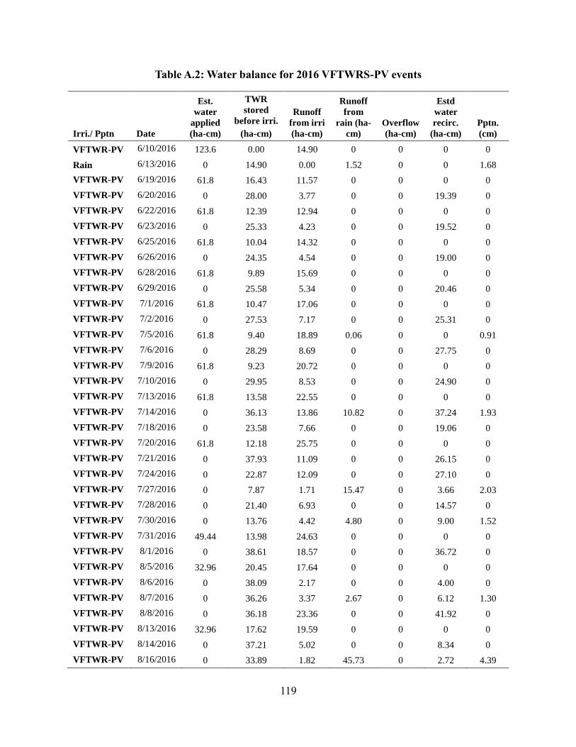
119

Table A.2: Water balance for 2016 VFTWRS-PV events

Irri./ Pptn Date

Est.

water

applied

(ha-cm)

TWR

stored

before irri.

(ha-cm)

Runoff

from irri

(ha-cm)

Runoff

from

rain (ha-

cm)

Overflow

(ha-cm)

Estd

water

recirc.

(ha-cm)

Pptn.

(cm)

VFTWR-PV 6/10/2016 123.6 0.00 14.90 0 0 0 0

Rain 6/13/2016 0 14.90 0.00 1.52 0 0 1.68

VFTWR-PV 6/19/2016 61.8 16.43 11.57 0 0 0 0

VFTWR-PV 6/20/2016 0 28.00 3.77 0 0 19.39 0

VFTWR-PV 6/22/2016 61.8 12.39 12.94 0 0 0 0

VFTWR-PV 6/23/2016 0 25.33 4.23 0 0 19.52 0

VFTWR-PV 6/25/2016 61.8 10.04 14.32 0 0 0 0

VFTWR-PV 6/26/2016 0 24.35 4.54 0 0 19.00 0

VFTWR-PV 6/28/2016 61.8 9.89 15.69 0 0 0 0

VFTWR-PV 6/29/2016 0 25.58 5.34 0 0 20.46 0

VFTWR-PV 7/1/2016 61.8 10.47 17.06 0 0 0 0

VFTWR-PV 7/2/2016 0 27.53 7.17 0 0 25.31 0

VFTWR-PV 7/5/2016 61.8 9.40 18.89 0.06 0 0 0.91

VFTWR-PV 7/6/2016 0 28.29 8.69 0 0 27.75 0

VFTWR-PV 7/9/2016 61.8 9.23 20.72 0 0 0 0

VFTWR-PV 7/10/2016 0 29.95 8.53 0 0 24.90 0

VFTWR-PV 7/13/2016 61.8 13.58 22.55 0 0 0 0

VFTWR-PV 7/14/2016 0 36.13 13.86 10.82 0 37.24 1.93

VFTWR-PV 7/18/2016 0 23.58 7.66 0 0 19.06 0

VFTWR-PV 7/20/2016 61.8 12.18 25.75 0 0 0 0

VFTWR-PV 7/21/2016 0 37.93 11.09 0 0 26.15 0

VFTWR-PV 7/24/2016 0 22.87 12.09 0 0 27.10 0

VFTWR-PV 7/27/2016 0 7.87 1.71 15.47 0 3.66 2.03

VFTWR-PV 7/28/2016 0 21.40 6.93 0 0 14.57 0

VFTWR-PV 7/30/2016 0 13.76 4.42 4.80 0 9.00 1.52

VFTWR-PV 7/31/2016 49.44 13.98 24.63 0 0 0 0

VFTWR-PV 8/1/2016 0 38.61 18.57 0 0 36.72 0

VFTWR-PV 8/5/2016 32.96 20.45 17.64 0 0 0 0

VFTWR-PV 8/6/2016 0 38.09 2.17 0 0 4.00 0

VFTWR-PV 8/7/2016 0 36.26 3.37 2.67 0 6.12 1.30

VFTWR-PV 8/8/2016 0 36.18 23.36 0 0 41.92 0

VFTWR-PV 8/13/2016 32.96 17.62 19.59 0 0 0 0

VFTWR-PV 8/14/2016 0 37.21 5.02 0 0 8.34 0

VFTWR-PV 8/16/2016 0 33.89 1.82 45.73 0 2.72 4.39

120

Table A.2: Water balance for 2016 VFTWRS-PV events (Cont.)

Irri./ Pptn Date

Est.

water

applied

(ha-cm)

TWR

stored

before irri.

(ha-cm)

Runoff

from irri

(ha-cm)

Runoff

from

rain (ha-

cm)

Overflow

(ha-cm)

Estd

water

recirc.

(ha-cm)

Pptn.

(cm)

VFTWR-PV 8/17/2016 0 39.55 31.72 0 40.03 46.93 0

VFTWR-PV 8/25/2016 20.6 24.34 15.14 0 0 0 0

VFTWR-PV 8/26/2016 0 39.48 35.01 0 0 47.15 0

Total 816 23 (Avg) 472 81 40 487 14

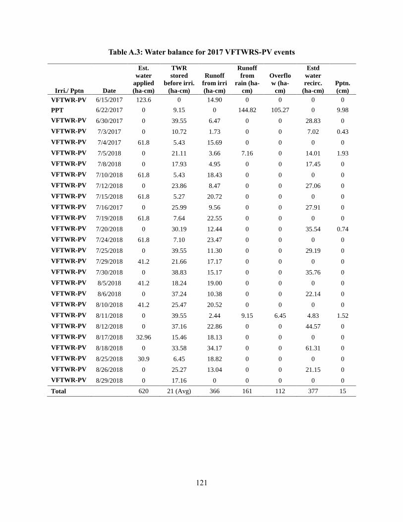
121

Table A.3: Water balance for 2017 VFTWRS-PV events

Irri./ Pptn Date

Est.

water

applied

(ha-cm)

TWR

stored

before irri.

(ha-cm)

Runoff

from irri

(ha-cm)

Runoff

from

rain (ha-

cm)

Overflo

w (ha-

cm)

Estd

water

recirc.

(ha-cm)

Pptn.

(cm)

VFTWR-PV 6/15/2017 123.6 0 14.90 0 0 0 0

PPT 6/22/2017 0 9.15 0 144.82 105.27 0 9.98

VFTWR-PV 6/30/2017 0 39.55 6.47 0 0 28.83 0

VFTWR-PV 7/3/2017 0 10.72 1.73 0 0 7.02 0.43

VFTWR-PV 7/4/2017 61.8 5.43 15.69 0 0 0 0

VFTWR-PV 7/5/2018 0 21.11 3.66 7.16 0 14.01 1.93

VFTWR-PV 7/8/2018 0 17.93 4.95 0 0 17.45 0

VFTWR-PV 7/10/2018 61.8 5.43 18.43 0 0 0 0

VFTWR-PV 7/12/2018 0 23.86 8.47 0 0 27.06 0

VFTWR-PV 7/15/2018 61.8 5.27 20.72 0 0 0 0

VFTWR-PV 7/16/2017 0 25.99 9.56 0 0 27.91 0

VFTWR-PV 7/19/2018 61.8 7.64 22.55 0 0 0 0

VFTWR-PV 7/20/2018 0 30.19 12.44 0 0 35.54 0.74

VFTWR-PV 7/24/2018 61.8 7.10 23.47 0 0 0 0

VFTWR-PV 7/25/2018 0 39.55 11.30 0 0 29.19 0

VFTWR-PV 7/29/2018 41.2 21.66 17.17 0 0 0 0

VFTWR-PV 7/30/2018 0 38.83 15.17 0 0 35.76 0

VFTWR-PV 8/5/2018 41.2 18.24 19.00 0 0 0 0

VFTWR-PV 8/6/2018 0 37.24 10.38 0 0 22.14 0

VFTWR-PV 8/10/2018 41.2 25.47 20.52 0 0 0 0

VFTWR-PV 8/11/2018 0 39.55 2.44 9.15 6.45 4.83 1.52

VFTWR-PV 8/12/2018 0 37.16 22.86 0 0 44.57 0

VFTWR-PV 8/17/2018 32.96 15.46 18.13 0 0 0 0

VFTWR-PV 8/18/2018 0 33.58 34.17 0 0 61.31 0

VFTWR-PV 8/25/2018 30.9 6.45 18.82 0 0 0 0

VFTWR-PV 8/26/2018 0 25.27 13.04 0 0 21.15 0

VFTWR-PV 8/29/2018 0 17.16 0 0 0 0 0

Total 620 21 (Avg) 366 161 112 377 15

122

Table A.4: Water balance for 2016 TWR full width events

Date

Source

Avail.

water in

pit (ha-

cm)

Water

appl.

from

twr pit

(ha-cm)

Water

from

source

(ha-

cm)

Overf

low

(ha-

cm)

Water

applied

(ha-

cm)

Pptn

(cm)

Irri

efficienc

y, %

Expd.

RO

from irri

(ha-cm)

Expd.

RO

from

pptn.

(cm)

Total

runof

f (ha-

cm)

Evap. (ha-

cm)

Deep

perc. (ha-

cm)

6/10/2016 Twr 206 136 0 0 136 0 98.83 23 0 23 1.58 0

6/13/2016 Rain 90 0 0 0 0 1.68 N/A 0 0.0508 2 3.19 0

6/19/2016 Twr +

pump 88 78 41 0 119 0 98.22 25 0 25 2.12 0

6/23/2016 Pump 33 21 119 0 140 0 97.72 31 0 31 3.19 0

6/29/2016 Twr +

pump 41 29 99 0 127 0 97.51 35 0 35 3.19 0

7/5/2016 Rain 43 0 0 0 0 0.91 N/A 0 0.002 0 1.03 0

7/7/2016 Twr +

pump 41 31 74 0 105 0 96.59 35 0 35 3.60 0

7/14/2016 Pump 41 31 384 0 415 1.93 98.38 113 0.361 123 6.68 0.25

7/27/2016 Rain 173 0 0 0 0 2.03 N/A 0 0.516 14 1.54 11.84

7/30/2016 Rain 183 0 0 0 0 1.52 N/A 0 0.160 4 1.54 42.68

8/2/2016 Twr 183 138 0 0 138 0 97.39 68 0 68 1.44 25.66

8/5/2016 Twr 111 103 263 0 366 0.15 99.54 37 0 37 0.95 8.63

8/7/2016 Rain 206 0 0 0 0 1.30 N/A 0 0.089 2 1.91 8.63

8/11/2016 Twr +

pump 206 195 169 0 364 0.25 99.34 49 0 49 2.38 0

8/16/2016 Rain 206 0 0 14 0 4.39 N/A 0 1.524 43 5.74 0

8/28/2016 Twr +

pump 206 164 0 35 164 0 99.67 53 0 53 0.47 0.74

9/1/2016 Twr +

pump 140 125 0 0 125 0 99.31 76 0 76 0.42 0

Total 1,051 1,149 49 2,200 14.17 94.50 545 2.7 621 40.54 98

122

123

Table A.5: Water balance for 2017 TWR full width events

Date

Source

Avail.

water in

pit (ha-

cm)

Water

appl.

from

twr pit

(ha-

cm)

Water

from

sourc

e (ha-

cm)

Overf

low

(ha-

cm)

Water

applied

(ha-cm)

Pptn

(cm)

Irri

efficien

cy, %

Expd. RO

from irri

(ha-cm)

Expd.

RO from

pptn.

(cm)

Total

runoff

(ha-cm)

Evap. (ha-

cm)

Deep

perc.

(ha-cm)

6/15/2017 Twr 206 125 0 0 125 0 97.05 21 0 21 3.72 0

6/22/2017 Rain 97 0 0 0 0 9.98 N/A 0 5.588 156 4.24 0

6/30/2017 Twr 206 99 0 45 99 0 98.92 25 0 25 1.07 0

7/1/2018 Rain 132 0 0 0 0 0 N/A 0 0.006 0 1.03 0

7/3/2017 Rain 130 0 0 0 0 0 N/A 0 0 0 2.06 0

7/7/2017 Twr + rain 127 117 0 0 117 1.93 98.70 41 0.239 47 1.54 0

7/10/2017 Pump 49 41 45 0 86 0 98.21 27 0 27 1.54 0

7/13/2017 Twr 33 21 64 0 84 0.00 98.15 29 0 29 1.54 0.25

7/16/2017 Pump 39 31 152 0 183 0.00 98.05 64 0 64 2.57 11.84

7/21/2017 Pump 70 62 132 0 193 0.00 97.37 74 0 74 1.54 42.68

7/24/2017 Twr + rain

76 62 234 0 296 0 98.23 121 0 121 3.08 25.66

7/30/2017 Twr 130 105 0 0 105 0.13 96.39 47 0 47 3.08 8.63

8/5/2017 Twr + rain 68 62 173 0 234 0.00 98.48 117 0 117 2.86 8.63

8/11/2017 Twr 121 93 0 0 93 1.52 95.91 51 0.305 60 3.82 0

8/19/2017 Twr + rain 84 72 53 0 125 0.30 98.80 74 0 74 1.44 0

8/22/2017 Twr + rain 84 74 33 0 107 0 96.42 66 0 66 3.82 0.00

8/30/2017 Rain 72 0 0 0 0 0 N/A 0 4.318 121 0 0

Total 962 886 45 1,848 13.87 94.62 757 10.456 1,048 38.96 98

123

124

Table A.6: Water balance for 2016 TWR half width events

Date

Source

Avail.

water

in pit

(ha-

cm)

Water

appl. from

twr pit

(ha-cm)

Water

from

source

(ha-cm)

Overfl

ow

(ha-

cm)

Water

applied

(ha-cm)

Pptn

(cm)

Irri

efficien

cy, %

Expd.

RO

from irri

(ha-cm)

Expd. RO

from

pptn.

(cm)

Total

runof

f (ha-

cm)

Evap. (ha-

cm)

Deep

perc. (ha-

cm)

6/10/2016 TWR 123 115 21 0 136 0 99.30 23 0 23 0.95 0

6/13/2016 Rain 31 0 0 0 0 1.68 N/A 0 0.051 2 1.91 0

6/19/2016 TWR +

pump 31 21 99 0 119 0 98.93 25 0 25 1.27 0

6/23/2016 Pump 33 21 119 0 140 0 98.64 31 0 31 1.91 0

6/29/2016 TWR +

pump 41 29 99 0 127 0 98.51 35 0 35 1.91 0

7/5/2016 Rain 45 0 0 0 0 0.91 N/A 0 0 0 0.62 0

7/7/2016 TWR +

pump 43 31 74 0 105 0 97.96 35 0 35 2.16 0

7/14/2016 Pump 45 31 389 0 419 1.93 99.04 158 0.356 169 4.01 0.25

7/27/2016 Rain 123 0 0 27 0 2.03 N/A 0 0.508 14 0.93 12.34

7/30/2016 Rain 123 0 0 12 0 1.52 N/A 0 0.152 4 0.93 44.16

8/2/2016 TWR 123 111 27 0 138 0 97.76 70 0 70 0.86 26.40

8/5/2016 TWR 78 68 300 0 368 0.15 99.64 199 0 199 0.58 8.88

8/7/2016 Rain 123 0 0 82 0 1.30 N/A 0 0.102 2 1.15 8.88

8/11/2016 TWR +

pump 123 113 253 0 366 0.25 99.61 214 0 214 1.42 0

8/16/2016 Rain 123 0 0 99 0 4.39 N/A 0 1.524 43 3.43 0

8/28/2016 TWR +

pump 123 113 53 25 167 0 99.79 101 0 101 0.29 0.74

9/1/2016 TWR +

pump 109 103 23 0 125 0 99.31 76 0 76 0 0

Total 754 1,456 245 2,210 14.17 88.56 966 2.692 1,042 24.32 102

124

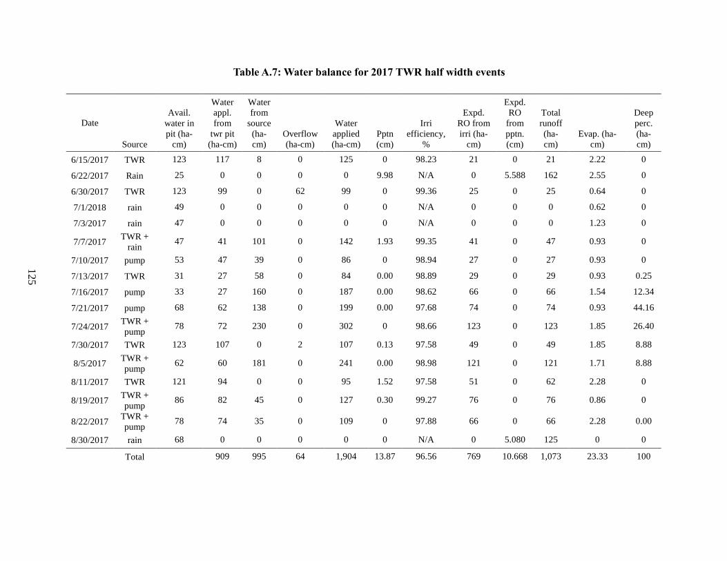
125

Table A.7: Water balance for 2017 TWR half width events

Date

Source

Avail.

water in

pit (ha-

cm)

Water

appl.

from

twr pit

(ha-cm)

Water

from

source

(ha-

cm)

Overflow

(ha-cm)

Water

applied

(ha-cm)

Pptn

(cm)

Irri

efficiency,

%

Expd.

RO from

irri (ha-

cm)

Expd.

RO

from

pptn.

(cm)

Total

runoff

(ha-

cm)

Evap. (ha-

cm)

Deep

perc.

(ha-

cm)

6/15/2017 TWR 123 117 8 0 125 0 98.23 21 0 21 2.22 0

6/22/2017 Rain 25 0 0 0 0 9.98 N/A 0 5.588 162 2.55 0

6/30/2017 TWR 123 99 0 62 99 0 99.36 25 0 25 0.64 0

7/1/2018 rain 49 0 0 0 0 0 N/A 0 0 0 0.62 0

7/3/2017 rain 47 0 0 0 0 0 N/A 0 0 0 1.23 0

7/7/2017 TWR +

rain 47 41 101 0 142 1.93 99.35 41 0 47 0.93 0

7/10/2017 pump 53 47 39 0 86 0 98.94 27 0 27 0.93 0

7/13/2017 TWR 31 27 58 0 84 0.00 98.89 29 0 29 0.93 0.25

7/16/2017 pump 33 27 160 0 187 0.00 98.62 66 0 66 1.54 12.34

7/21/2017 pump 68 62 138 0 199 0.00 97.68 74 0 74 0.93 44.16

7/24/2017 TWR +

pump 78 72 230 0 302 0 98.66 123 0 123 1.85 26.40

7/30/2017 TWR 123 107 0 2 107 0.13 97.58 49 0 49 1.85 8.88

8/5/2017 TWR +

pump 62 60 181 0 241 0.00 98.98 121 0 121 1.71 8.88

8/11/2017 TWR 121 94 0 0 95 1.52 97.58 51 0 62 2.28 0

8/19/2017 TWR +

pump 86 82 45 0 127 0.30 99.27 76 0 76 0.86 0

8/22/2017 TWR +

pump 78 74 35 0 109 0 97.88 66 0 66 2.28 0.00

8/30/2017 rain 68 0 0 0 0 0 N/A 0 5.080 125 0 0

Total 909 995 64 1,904 13.87 96.56 769 10.668 1,073 23.33 100

125

126

Table A.8 (a): Capital cost calculation (in $) for each base case scenario

Description Unit Pump + layflat pipe

Pump + underground piping

(12") Pump + Solar+layflat pipe

Cost per

unit

No. of

unit Total cost

Cost per

unit

No. of

unit Total cost

Cost per

unit

No. of

unit Total cost

Pump each $4,050.50 1 $4,050.50 $4,050.50 1 $4,050.50 $4,050.50 1 $4,050.50

Pump panel each $5,386.00 1 $5,386.00 $5,386.00 1 $5,386.00 $5,386.00 1 $5,386.00

Utility each $1,000.00 1 $1,000.00 $1,000.00 1 $1,000.00 $1,000.00 0 $0.00

Culvert

VF

-TW

R (

Pum

p)

each $433.00 1 $15.00 $433.00 1 $433.00 $433.00 1 $433.00

1/4" steel plate 4' by 4' sheet metal each $100.00 2 $200.00 $100.00 2 $200.00 $100.00 2 $200.00

Pump fabrication labor hours $20.00 24 $480.00 $20.00 24 $480.00 $20.00 24 $480.00

Field installation hours $20.00 6 $120.00 $20.00 6 $120.00 $20.00 6 $120.00

Pressure transducer for depth each $120.00 1 $120.00 $120.00 1 $120.00 $120.00 1 $120.00

PVC and hardware for sensor and standpipe each $50.00 1 $50.00 $50.00 1 $50.00 $50.00 1 $50.00

2" by 2" 1/8" angle iron for support ft $2.58 12 $30.90 $2.58 12 $30.90 $2.58 12 $30.90

Ladder (optional) each $20.00 1 $20.00 $20.00 1 $20.00 $20.00 1 $20.00

Standpipe steel (used pipe) each $100.00 1 $100.00 $100.00 1 $100.00 $100.00 1 $100.00

Flanges 8" each $22.65 2 $45.30 $22.65 2 $45.30 $22.65 2 $45.30

Flange gaskets each $2.50 2 $5.00 $2.50 2 $5.00 $2.50 2 $5.00

bolts 3/4 hex by 3" each $0.95 12 $11.40 $0.95 12 $11.40 $0.95 12 $11.40

nuts 3/4" each $0.20 12 $2.40 $0.20 12 $2.40 $0.20 12 $2.40

8" check valve (drainage agri-drain) each $227.40 1 $227.40 $227.40 1 $227.40 $227.40 1 $227.40

Primer, paint and epoxy coating $55.00 $55.00 $55.00

bolts 1/2" by 1.5" (panel) each $0.22 4 $0.87 $0.22 4 $0.87 $0.22 4 $0.87

nuts 1/2" (panel) each $0.07 4 $0.26 $0.07 4 $0.26 $0.07 4 $0.26

hardware fabric for sump 19g 1/4" ft $0.35 12 $4.20 $0.35 12 $4.20 $0.35 12 $4.20

PVC paint $0.50 5.99 $3.00 $0.50 5.99 $3.00 $0.50 5.99 $3.00

washers 1/2" each $0.08 8 $0.64 $0.08 8 $0.64 $0.08 8 $0.64

126

127

Table A.8 (a): Capital cost calculation (in $) for each base case scenario (Cont.)

Description Unit Pump + layflat pipe

Pump + underground piping

(12") Pump + Solar+layflat pipe

Cost per

unit

No. of

unit Total cost

Cost per

unit

No. of

unit Total cost

Cost per

unit

No. of

unit Total cost

3/4" conduit, connectors and wire for motor $50.00 $50.00 $50.00

Fronius Galvo 3.1-1 inverter

Sola

r S

truct

ure

each $0.00 0 $0.00 $0.00 0 $0.00 $1,800.00 1 $1,800.00

Mitbushi 265 panels (PV-MjE265FB) each $0.00 0 $0.00 $0.00 0 $0.00 $214.50 12 $2,574.00

4 x 4 x 5/16 square tubing (frame) ft $0.00 0 $0.00 $0.00 0 $0.00 $8.71 130 $1,132.30

4x1/2 flat bar ft $0.00 0 $0.00 $0.00 0 $0.00 $2.82 3 $8.46

1 x 1, 1/8" SQ tube ft $0.00 0 $0.00 $0.00 0 $0.00 $0.69 142 $97.98

2 x 2 square tubing (uprights) 3/16" ft $0.00 0 $0.00 $0.00 0 $0.00 $2.09 28 $58.52

Steel rod solid 1" ft $0.00 0 $0.00 $0.00 0 $0.00 $3.92 1.81 $7.10

4 x 4 x 5/16 square tubing (3 pt) ft $0.00 0 $0.00 $0.00 0 $0.00 $8.71 12 $104.52

Solar wire and connectors each $0.00 0 $0.00 $0.00 0 $0.00 $0.36 50 $18.00

MC4 Solar connectors each $0.00 0 $0.00 $0.00 0 $0.00 $1.40 2 $2.80

Tamper resis. bolts 18-8 SS, 3/8"-16, 2" each $0.00 0 $0.00 $0.00 0 $0.00 $2.06 96 $197.76


tamper resistant nuts, 3/8" sloped nuts each $0.00 0 $0.00 $0.00 0 $0.00 $1.05 108 $113.40

SS washers each $0.00 0 $0.00 $0.00 0 $0.00 $0.32 108 $34.56

SS nylon lock nuts 3/8"-16 each $0.00 0 $0.00 $0.00 0 $0.00 $0.31 12 $3.66

SS cap screws 3/8"-16, 3.5" each $0.00 0 $0.00 $0.00 0 $0.00 $0.18 12 $2.16

Primer and paint for solar panels $0.00 0 $0.00 $0.00 0 $0.00 $55.00

Labor for solar panel fabrication hours $0.00 0 $0.00 $0.00 0 $0.00 $20.00 40 $800.00

Wire from electric source to pump, 4 Quad ft $1.03 200 $206.00 $1.03 200 $206.00 $1.03 0 $0.00

Irrigation pipeline, 12 in ft $0.00 0 $0.00 $7.80 1232 $9,609.60 $0.00 0 $0.00

Drainline ft $7.80 290 $2,262.00 $7.80 290 $2,262.00 $7.80 290 $2,262.00

Earthwork for pit cy $0.00 0 $0.00 $0.00 0 $0.00 $0.00 0 $0.00

Total cost $14,445.87 $24,473.47 $20,725.69

127

128

Table A.8 (b): Capital cost calculation (in $) for each base case scenario

Description Unit Pump + Solar+ underground pipe TWR (full length) TWR (half length)

Cost per

unit

No. of

unit Total cost

Cost per

unit

No. of

unit Total cost

Cost per

unit

No. of

unit Total cost

Pump each $4,050.50 1 $4,050.50 $22,508.00 1 $22,508.00

$22,508.0

0 1 $22,508.00

Pump panel each $5,386.00 1 $5,386.00 $0.00 0 $0.00 $0.00 0 $0.00

Utility each $1,000.00 0 $0.00 $1,000.00 1 $1,000.00 $1,000.00 1 $1,000.00

Culvert

VF

-TW

R (

Pum

p)

each $433.00 1 $433.00 $0.00 0 $0.00 $0.00 0 $0.00

1/4" steel plate 4' by 4' sheet metal each $100.00 2 $200.00 $0.00 0 $0.00 $0.00 0 $0.00

Pump fabrication labor hours $20.00 24 $480.00 $0.00 0 $0.00 $0.00 0 $0.00

Field installation hours $20.00 6 $120.00 $0.00 0 $0.00 $0.00 0 $0.00

Pressure transducer for depth each $120.00 1 $120.00 $0.00 0 $0.00 $0.00 0 $0.00

PVC and hardware for sensor and standpipe each $50.00 1 $50.00 $0.00 0 $0.00 $0.00 0 $0.00

2" by 2" 1/8" angle iron for support ft $2.58 12 $30.90 $0.00 0 $0.00 $0.00 0 $0.00

Ladder (optional) each $20.00 1 $20.00 $0.00 0 $0.00 $0.00 0 $0.00

Standpipe steel (used pipe) each $100.00 1 $100.00 $0.00 0 $0.00 $0.00 0 $0.00

Flanges 8" each $22.65 2 $45.30 $0.00 0 $0.00 $0.00 0 $0.00

Flange gaskets each $2.50 2 $5.00 $0.00 0 $0.00 $0.00 0 $0.00

bolts 3/4 hex by 3" each $0.95 12 $11.40 $0.00 0 $0.00 $0.00 0 $0.00

nuts 3/4" each $0.20 12 $2.40 $0.00 0 $0.00 $0.00 0 $0.00

8" check valve (drainage agri-drain) each $227.40 1 $227.40 $0.00 0 $0.00 $0.00 0 $0.00

Primer, paint and epoxy coating $55.00 $0.00 0 $0.00 $0.00 0 $0.00

bolts 1/2" by 1.5" (panel) each $0.22 4 $0.87 $0.00 0 $0.00 $0.00 0 $0.00

nuts 1/2" (panel) each $0.07 4 $0.26 $0.00 0 $0.00 $0.00 0 $0.00

washers 1/2" each $0.08 8 $0.64 $0.00 0 $0.00 $0.00 0 $0.00

3/4" conduit, connectors and wire for motor $50.00 $0.00 0 $0.00 $0.00 0 $0.00

128

129

Table A.8 (b): Capital cost calculation (in $) for each base case scenario (Cont.)

Description Unit Pump + Solar+ underground pipe TWR (full length) TWR (half length)

Cost per

unit

No. of

unit Total cost

Cost per

unit

No. of

unit Total cost

Cost per

unit

No. of

unit Total cost

hardware fabric for sump 19g 1/4" ft $0.35 12 $4.20 $0.00 0 $0.00 $0.00 0 $0.00

PVC paint $0.50 5.99 $3.00 $0.00 0 $0.00 $0.00 0 $0.00

Fronius Galvo 3.1-1 inverter

Sola

r S

truct

ure

each $1,800.00 1 $1,800.00 $0.00 0 $0.00 $0.00 0 $0.00

Mitbushi 265 panels (PV-MjE265FB) each $214.50 12 $2,574.00 $0.00 0 $0.00 $0.00 0 $0.00

4 x 4 x 5/16 square tubing (frame) ft $8.71 130 $1,132.30 $0.00 0 $0.00 $0.00 0 $0.00

4x1/2 flat bar ft $2.82 3 $8.46 $0.00 0 $0.00 $0.00 0 $0.00

1 x 1, 1/8" SQ tube ft $0.69 142 $97.98 $0.00 0 $0.00 $0.00 0 $0.00

2 x 2 square tubing (uprights) 3/16" ft $2.09 28 $58.52 $0.00 0 $0.00 $0.00 0 $0.00

Steel rod solid 1" ft $3.92 1.81 $7.10 $0.00 0 $0.00 $0.00 0 $0.00

4 x 4 x 5/16 square tubing (3 pt) ft $8.71 12 $104.52 $0.00 0 $0.00 $0.00 0 $0.00

Solar wire and connectors each $0.36 50 $18.00 $0.00 0 $0.00 $0.00 0 $0.00

MC4 Solar connectors each $1.40 2 $2.80 $0.00 0 $0.00 $0.00 0 $0.00



tamper resistant nuts, 3/8" sloped nuts each $1.05 108 $113.40 $0.00 0 $0.00 $0.00 0 $0.00

SS washers each $0.32 108 $34.56 $0.00 0 $0.00 $0.00 0 $0.00

SS nylon lock nuts 3/8"-16 each $0.31 12 $3.66 $0.00 0 $0.00 $0.00 0 $0.00

SS cap screws 3/8"-16, 3.5" each $0.18 12 $2.16 $0.00 0 $0.00 $0.00 0 $0.00

Primer and paint for solar panels $55.00 $0.00 0 $0.00 $0.00 0 $0.00

Labor for solar panel fabrication hours $20.00 40 $800.00 $0.00 0 $0.00 $0.00 0 $0.00

Wire from electric source to pump, 4 Quad ft $1.03 0 $0.00 $1.03 200 $206.00 $1.03 200 $206.00

Irrigation pipeline, 12 in ft $7.80 1232 $9,609.60 $7.80 1232 $9,609.60 $7.80 1232 $9,609.60

Drainline ft $7.80 290 $2,262.00 $7.80 290 $2,262.00 $7.80 174 $1,357.20

Earthwork for pit cy $0.00 $0.00 $1.19 16370 $19,480.30 $1.19 8185 $9,740.15

Total cost $30,335.29 $55,065.90 $44,420.95

129

130

Table A.9: Net present value on per acre basis (NPV) at 5% interest rate and discounted payback period (DPP in year) for

each scenario at 5% discount rate for surface water

Scenarios NPV DPP,

years

NPV DPP,

years

Scenarios NPV DPP,

years

NPV DPP,

years Surface water source Groundwater source Surface water source Groundwater source

1 $3,250 1.80 $2,736 1.89 1-2000 ft $3,199 2.04 $2,686 2.15

2 $3,165 2.97 $2,633 3.12 2-2000 ft $3,115 3.22 $2,583 3.39

3 $3,126 2.60 $2,502 2.83 5-2000 ft $1,816 9.52 $1,312 10.21

4 $3,052 3.71 $2,410 3.99 6-2000 ft $2,287 6.79 $1,740 7.33

5 $1,869 9.12 $1,365 9.66 1-2500 ft $3,168 2.19 $2,654 2.31

6 $2,339 6.48 $1,792 6.93 2-2500 ft $3,084 3.38 $2,552 3.55

7 $1,717 9.52 $1,231 9.74 5-2500 ft $1,782 9.77 $1,278 10.48

8 $2,236 6.56 $1,697 7.05 6-2500 ft $1,905 6.99 $1,708 7.55

1-500 ft $3,241 1.84 $2,728 1.93 1-3000 ft $3,150 2.28 $2,637 2.40

2-500 ft $3,157 3.01 $2,625 3.17 2-3000 ft $3,066 3.46 $2,534 3.64

5-500 ft $1,860 9.19 $1,356 9.85 5-3000 ft $1,763 9.90 $1,259 10.63

6-500 ft $2,331 6.53 $1,783 7.03 6-3000 ft $2,237 7.11 $1,690 7.67

1-1000 ft $3,227 1.90 $2,714 2.00 1-3500 ft $3,093 2.56 $2,580 2.70

2-1000 ft $3,143 3.08 $2,611 3.24 2-3500 ft $3,009 3.75 $2,477 3.94

5-1000 ft $1,845 9.30 $1,341 9.96 5-3500 ft $1,702 10.37 $1,198 11.14

6-1000 ft $2,316 6.62 $1,769 7.13 6-3500 ft $2,178 7.49 $1,631 8.08

1-1500 ft $3,213 1.97 $2,700 2.07 1-4000 ft $3,070 2.68 $2,557 2.82

2-1500 ft $3,129 3.15 $2,597 3.32 2-4000 ft $2,986 3.86 $2,454 4.06

5-1500 ft $1,831 9.41 $1,326 10.08 5-4000 ft $1,678 10.56 $1,173 11.35

6-1500 ft $1,952 6.71 $1,755 7.23 6-4000 ft $2,154 7.65 $1,607 8.25

130

131



Scenarios NPV DPP,

years

NPV DPP,

years

Scenarios NPV DPP,

years

NPV DPP,


1 $3,250 1.82 $2,445 1.92 1-2000 ft $3,199 2.07 $2,395 2.18

2 $3,165 3.03 $2,327 3.19 2-2000 ft $3,115 3.29 $2,277 3.47

3 $3,126 2.64 $2,217 2.89 5-2000 ft $1,816 10.13 $1,037 10.91

4 $3,052 3.80 $2,110 4.08 6-2000 ft $2,287 7.09 $1,458 7.68

5 $1,869 9.67 $1,090 10.19 1-2500 ft $3,168 2.23 $2,364 2.35

6 $2,339 6.75 $1,510 7.20 2-2500 ft $3,084 3.46 $2,245 3.64

7 $1,717 10.13 $972 10.19 5-2500 ft $1,782 10.41 $1,003 11.23

8 $2,236 6.84 $1,427 7.33 6-2500 ft $2,255 7.32 $1,426 7.92

1-500 ft $3,241 1.86 $2,437 1.96 1-3000 ft $3,150 2.32 $2,346 2.44

2-500 ft $3,157 3.08 $2,319 3.24 2-3000 ft $3,066 3.54 $2,228 3.73

5-500 ft $1,860 9.76 $1,081 10.51 5-3000 ft $1,763 10.57 $984 11.41

6-500 ft $2,331 6.80 $1,501 7.36 6-3000 ft $2,237 7.44 $1,408 8.05

1-1000 ft $3,227 1.93 $2,423 2.03 1-3500 ft $3,093 2.61 $2,289 2.75

2-1000 ft $3,143 3.15 $2,305 3.32 2-3500 ft $3,009 3.84 $2,171 4.04

5-1000 ft $1,845 9.88 $1,066 10.65 5-3500 ft $1,702 11.10 $923 12.00

6-1000 ft $2,316 6.90 $1,487 7.46 6-3500 ft $2,178 7.86 $1,349 8.52

1-1500 ft $3,213 2.00 $2,409 2.11 1-4000 ft $3,070 2.73 $2,266 2.88

2-1500 ft $3,129 3.22 $2,291 3.39 2-4000 ft $2,986 3.96 $2,148 4.18

5-1500 ft $1,831 10.00 $1,052 10.78 5-4000 ft $1,678 11.33 $899 12.25

6-1500 ft $2,302 6.99 $1,473 7.57 6-4000 ft $2,154 8.02 $1,325 8.71

131

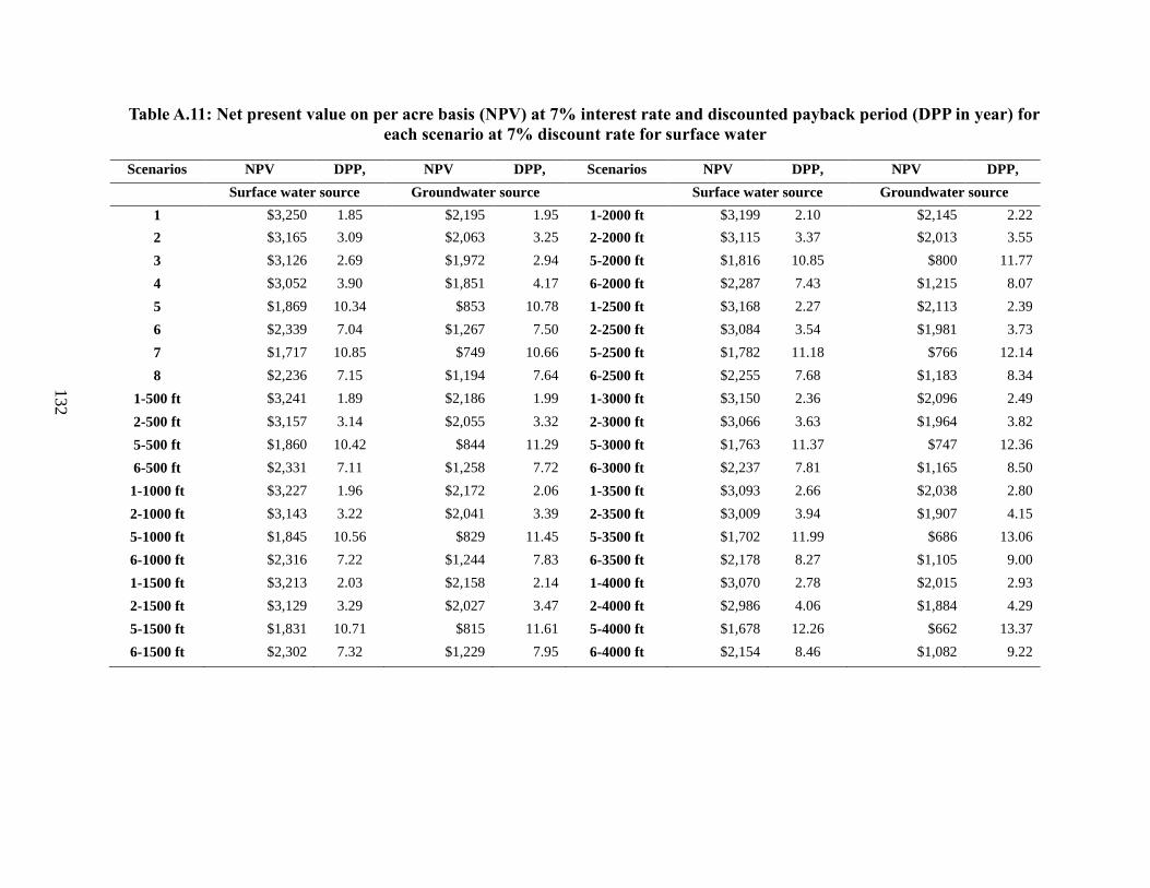
132



Scenarios NPV DPP,

years

NPV DPP,

years

Scenarios NPV DPP,

years

NPV DPP,


1 $3,250 1.85 $2,195 1.95 1-2000 ft $3,199 2.10 $2,145 2.22

2 $3,165 3.09 $2,063 3.25 2-2000 ft $3,115 3.37 $2,013 3.55

3 $3,126 2.69 $1,972 2.94 5-2000 ft $1,816 10.85 $800 11.77

4 $3,052 3.90 $1,851 4.17 6-2000 ft $2,287 7.43 $1,215 8.07

5 $1,869 10.34 $853 10.78 1-2500 ft $3,168 2.27 $2,113 2.39

6 $2,339 7.04 $1,267 7.50 2-2500 ft $3,084 3.54 $1,981 3.73

7 $1,717 10.85 $749 10.66 5-2500 ft $1,782 11.18 $766 12.14

8 $2,236 7.15 $1,194 7.64 6-2500 ft $2,255 7.68 $1,183 8.34

1-500 ft $3,241 1.89 $2,186 1.99 1-3000 ft $3,150 2.36 $2,096 2.49

2-500 ft $3,157 3.14 $2,055 3.32 2-3000 ft $3,066 3.63 $1,964 3.82

5-500 ft $1,860 10.42 $844 11.29 5-3000 ft $1,763 11.37 $747 12.36

6-500 ft $2,331 7.11 $1,258 7.72 6-3000 ft $2,237 7.81 $1,165 8.50

1-1000 ft $3,227 1.96 $2,172 2.06 1-3500 ft $3,093 2.66 $2,038 2.80

2-1000 ft $3,143 3.22 $2,041 3.39 2-3500 ft $3,009 3.94 $1,907 4.15

5-1000 ft $1,845 10.56 $829 11.45 5-3500 ft $1,702 11.99 $686 13.06

6-1000 ft $2,316 7.22 $1,244 7.83 6-3500 ft $2,178 8.27 $1,105 9.00

1-1500 ft $3,213 2.03 $2,158 2.14 1-4000 ft $3,070 2.78 $2,015 2.93

2-1500 ft $3,129 3.29 $2,027 3.47 2-4000 ft $2,986 4.06 $1,884 4.29

5-1500 ft $1,831 10.71 $815 11.61 5-4000 ft $1,678 12.26 $662 13.37

6-1500 ft $2,302 7.32 $1,229 7.95 6-4000 ft $2,154 8.46 $1,082 9.22

132

133



Scenarios NPV DPP,

years

NPV DPP,

years

Scenarios NPV DPP,

years

NPV DPP,


1 $3,250 1.87 $1,978 1.97 1-2000 ft $3,199 2.14 $1,927 2.26

2 $3,165 3.16 $1,834 3.32 2-2000 ft $3,115 3.45 $1,784 3.63

3 $3,126 2.74 $1,759 3.00 5-2000 ft $1,816 11.72 $594 12.83

4 $3,052 3.99 $1,627 4.26 6-2000 ft $2,287 7.80 $1,004 8.52

5 $1,869 11.11 $648 11.41 1-2500 ft $3,168 2.31 $1,896 2.43

6 $2,339 7.39 $1,056 7.81 2-2500 ft $3,084 3.62 $1,753 3.82

7 $1,717 11.73 $555 11.15 5-2500 ft $1,782 12.11 $561 13.29

8 $2,236 7.50 $993 7.96 6-2500 ft $2,255 8.07 $972 8.82

1-500 ft $3,241 1.92 $1,969 2.02 1-3000 ft $3,150 2.40 $1,879 2.53

2-500 ft $3,157 3.21 $1,826 3.39 2-3000 ft $3,066 3.72 $1,735 3.92

5-500 ft $1,860 11.22 $639 12.25 5-3000 ft $1,763 12.34 $542 13.55

6-500 ft $2,331 7.46 $1,048 8.12 6-3000 ft $2,237 8.23 $954 8.99

1-1000 ft $3,227 1.99 $1,955 2.10 1-3500 ft $3,093 2.71 $1,821 2.86

2-1000 ft $3,143 3.29 $1,812 3.47 2-3500 ft $3,009 4.04 $1,678 4.27

5-1000 ft $1,845 11.38 $624 12.45 5-3500 ft $1,702 13.10 $481 14.44

6-1000 ft $2,316 7.57 $1,033 8.25 6-3500 ft $2,178 8.74 $895 9.58

1-1500 ft $3,213 2.06 $1,941 2.18 1-4000 ft $3,070 2.83 $1,798 2.99

2-1500 ft $3,129 3.37 $1,798 3.55 2-4000 ft $2,986 4.18 $1,655 4.42

5-1500 ft $1,831 11.55 $609 12.64 5-4000 ft $1,678 13.43 $456 14.81

6-1500 ft $2,302 7.69 $1,019 8.39 6-4000 ft $2,154 8.95 $871 9.82

133

134



Scenarios NPV DPP,

years

NPV DPP,

years

Scenarios NPV DPP,

years

NPV DPP,


1 $3,250 1.90 $1,789 2.00 1-2000 ft $3,199 2.17 $1,738 2.29

2 $3,165 3.22 $1,635 3.39 2-2000 ft $3,115 3.53 $1,585 3.72

3 $3,126 2.80 $1,574 3.06 5-2000 ft $1,816 12.81 $416 14.20

4 $3,052 4.10 $1,431 4.35 6-2000 ft $2,287 8.23 $821 9.03

5 $1,869 12.07 $469 12.09 1-2500 ft $3,168 2.35 $1,707 2.48

6 $2,339 7.76 $873 8.15 2-2500 ft $3,084 3.71 $1,553 3.91

7 $1,717 12.82 $386 11.67 5-2500 ft $1,782 13.30 $382 14.79

8 $2,236 7.88 $817 8.30 6-2500 ft $2,255 8.54 $789 9.39

1-500 ft $3,241 1.94 $1,780 2.05 1-3000 ft $3,150 2.44 $1,689 2.58

2-500 ft $3,157 3.29 $1,627 3.47 2-3000 ft $3,066 3.81 $1,536 4.02

5-500 ft $1,860 12.20 $460 13.47 5-3000 ft $1,763 13.59 $363 15.12

6-500 ft $2,331 7.84 $864 8.59 6-3000 ft $2,237 8.71 $771 9.58

1-1000 ft $3,227 2.02 $1,766 2.13 1-3500 ft $3,093 2.76 $1,632 2.91

2-1000 ft $3,143 3.37 $1,613 3.56 2-3500 ft $3,009 4.14 $1,479 4.40

5-1000 ft $1,845 12.40 $445 13.71 5-3500 ft $1,702 14.55 $302 16.30

6-1000 ft $2,316 7.96 $850 8.73 6-3500 ft $2,178 9.29 $711 10.25

1-1500 ft $3,213 2.09 $1,752 2.21 1-4000 ft $3,070 2.89 $1,609 3.05

2-1500 ft $3,129 3.45 $1,599 3.64 2-4000 ft $2,986 4.30 $1,456 4.55

5-1500 ft $1,831 12.61 $430 13.95 5-4000 ft $1,678 14.96 $277 16.81

6-1500 ft $2,302 8.09 $835 8.88 6-4000 ft $2,154 9.54 $688 10.54

134

135

Table A.14: Water balance for each irrigation event for 2016 to calculate deep percolation using GMS sensor values at 15 locations

M1 E1 W1 M2 E2 W2 M3 E3 W3 M4 E4 W4 M5 E5 W5 M1 E1 W1 M2 E2 W2 M3 E3 W3 M4 E4 W4 M5 E5 W5

CF 6/10/2016 1.79 0.00 0.30 0.39 N/A N/A N/A N/A N/A N/A N/A N/A N/A N/A N/A N/A N/A N/A N/A N/A N/A N/A N/A N/A N/A N/A N/A N/A N/A N/A N/A N/A N/A N/A N/A

CF 6/19/2016 1.56 0.00 0.04 0.42 1.00 1.45 1.43 1.00 0.88 1.34 1.81 1.49 1.62 1.73no

DP

no

DP1.76

no

DP0.88 0.10 -0.35 -0.33 0.11 0.23 -0.23 -0.71 -0.39 -0.51 -0.62

no

DP

no

DP-0.65

no

DP0.23 0.04

CF 6/23/2016 1.84 0.00 0.33 0.62 0.54 0.86 0.70 0.61 0.52 0.57 0.74 1.03 0.49 1.09 0.64 0.59 1.12 1.21 1.17 0.35 0.03 0.19 0.28 0.37 0.32 0.15 -0.14 0.40 -0.20 0.25 0.30 -0.23 -0.32 -0.28 0.17

Surge 6/29/2016 1.68 0.00 0.07 0.80no

DP

no

DP1.33

no

DP

no

DP

no

DP

no

DP

no

DP1.47 0.82

no

DP1.57

no

DP1.34 0.67

no

DP

no

DP-0.51

no

DP

no

DP

no

DP

no

DP

no

DP-0.66 0.00

no

DP-0.75

no

DP-0.53 0.14 0.01

Pptn 7/5/2016 0.00 0.36 0.02 0.21no

DP

no

DP0.43

no

DP

no

DP

no

DP

no

DP

no

DP

no

dp

no

DP

no

DP

no

DP

no

DP

no

DP

no

dp

no

DP

no

DP-0.30

no

DP

no

DP

no

DP

no

DP

no

DP

no

DP

no

DP

no

DP

no

DP

no

DP

no

DP

no

DP0.00

Surge 7/7/2016 1.39 0.00 0.26 0.80no

DP

no

DP1.79

no

DP

no

DP

no

DP

no

DP

no

DP

no

DP

no

DP

no

DP

no

DP

no

DP

no

DP

no

dp

no

DP

no

DP-1.46

no

DP

no

DP

no

DP

no

DP

no

DP

no

DP

no

DP

no

DP

no

DP

no

DP

no

DP

no

DP0.00

VFTWRS 7/14/2016 3.90 0.76 0.49 2.99 1.02no

DP1.63

no

DP

no

DP2.61

no

DP

no

DP3.43

no

DP

no

DP1.63 2.19 1.72 1.96 0.16

no

DP-0.45

no

DP

no

DP-1.43

no

DP

no

DP-2.25

no

DP

no

DP-0.44 -1.01 -0.54 -0.78 0.01

Pptn 7/27/2016 0.00 0.80 0.18 0.28 0.76no

DP0.00

no

DP

no

DP1.25 1.38

no

DP1.38

no

DP

no

DP0.00

no

DP

no

DP

no

dp-0.42

no

DP0.34

no

DP

no

DP-0.91 -1.04

no

DP-1.04

no

DP

no

DP0.34

no

DP

no

DP

no

DP0.05

Pptn 7/30/2016 0.00 0.60 0.01 0.58 0.52no

DP0.68

no

DP

no

DP0.81

no

DP

no

DP0.97

no

DP

no

DP0.55

no

DP

no

DP

no

dp-0.51

no

DP-0.67

no

DP

no

DP-0.80

no

DP

no

DP-0.96

no

DP

no

DP-0.54

no

DP

no

DP

no

DP0.00

CF 8/2/2016 1.80 0.00 0.95 0.54 0.37no

DP0.56

no

DP

no

DP

no

DP

no

DP

no

DP

no

DP

no

DP

no

DP0.00

no

DP

no

DP

no

dp-0.06

no

DP-0.25

no

DP

no

DP

no

DP

no

DP

no

DP

no

DP

no

DP

no

DP0.31

no

DP

no

DP

no

DP0.02

VFTWRS 8/5/2016 0.96 0.06 0.18 0.39 1.06no

DP0.75

no

DP

no

DP

no

DP

no

DP

no

DP0.97

no

DP

no

DP

no

DP

no

DP2.06 1.03 -0.61

no

DP-0.30

no

DP

no

DP

no

DP

no

DP

no

DP-0.52

no

DP

no

DP

no

DP

no

DP-1.61 -0.58 0.00

Pptn 8/7/2016 0.00 0.51 0.34 0.12no

DP

no

DP0.00

no

DP

no

DP

no

DP

no

DP

no

DP0.00

no

DP

no

DP

no

DP

no

DP0.00 0.05

no

DP

no

DP0.05

no

DP

no

DP

no

DP

no

DP

no

DP0.05

no

DP

no

DP

no

DP

no

DP0.05 0.00 0.02

VFTWRS 8/11/2016 1.09 0.10 0.08 0.50 1.10no

DP1.25

no

DP

no

DP1.63 1.56

no

DP1.81 1.65

no

DP1.33 1.35 1.26 1.30 -0.49

no

DP-0.64

no

DP

no

DP-1.02 -0.95

no

DP-1.20 -1.04

no

DP-0.72 -0.74 -0.65 -0.69 0.00

VFTWRS 8/28/2016 1.18 0.00 0.08 0.42 N/A N/A N/A N/A N/A N/A N/A N/A N/Ano

DP

no

DP

no

DPN/A N/A N/A N/A N/A N/A N/A N/A N/A N/A N/A N/A

no

DP

no

DP

no

DPN/A N/A N/A N/A

Surge 9/1/2016 1.64 0.00 1.09 0.35no

DP

no

DP0.00

no

DP

no

DP

no

DP0.73

no

DP0.37

no

DP

no

DP0.04

no

DP

no

DP

no

dp

no

DP

no

DP0.20

no

DP

no

DP

no

DP-0.53

no

DP-0.17

no

DP

no

DP0.16

no

DP

no

DP

no

DP0.02

Soil moisture storage (in) Deep percolation (in)

Total

DP

(in)

IR/Pptn

(in)Date

IR (ac-

in/ac)

Pptn

(in)

RO

(in)

ET

(in)

135

136

Table A.15: Water balance for each irrigation event for 2017 to calculate deep percolation using GMS sensor values at 15 locations

M1 E1 W1 M2 E2 W2 M3 E3 W3 M4 E4 W4 M5 E5 W5 M1 E1 W1 M2 E2 W2 M3 E3 W3 M4 E4 W4 M5 E5 W5

VFTWRS

G06/15/17 1.65 0.00 0.12 0.31 1.16 1.14 1.18

no

DPN/A N/A N/A N/A N/A N/A

no

DPN/A N/A N/A 1.95 0.06 0.08 0.03

no

DPN/A N/A N/A N/A N/A N/A

no

DPN/A N/A N/A -0.74 N/A

VFTWRS

G06/30/17 0.89 0.00 0.00 0.35 1.74 1.56 1.65 1.58 1.43 1.94 1.08 1.27 1.62 1.68

no

DP2.42

no

DP

no

DP

no

DP-1.20 -1.02 -1.11 -1.04 -0.89 -1.40 -0.54 -0.73 -1.08 -1.14

no

DP-1.88

no

DP

no

DP

no

DP0.00

VFTWRS

G07/07/17 0.83 0.76 0.43 0.49 1.19 1.45 1.79 1.43 1.29 1.65 2.11 1.04 1.35 1.76 1.83 2.27 1.67 no dp 0.84 -0.52 -0.78 -1.12 -0.76 -0.62 -0.98 -1.44 -0.37 -0.68 -1.09 -1.16 -1.60 -1.00

no

DP-0.17 0.00

VFTWRS

S07/10/17 0.75 0.00 0.00 0.72

no

DP

no

DP0.53

no

DP0.37 0.57

no

DP0.20

no

DP

no

DP

no

DP

no

DP

no

DP

no

DP

no

DP

no

DP

no

DP-0.50

no

DP-0.34 -0.54

no

DP-0.17

no

DP

no

DP

no

DP

no

DP

no

DP

no

DP

no

DP0.00

VFTWRS

S07/13/17 0.87 0.00 0.00 0.45

no

DP

no

DP

no

DP

no

DP0.42 0.72

no

DP0.63

no

DP

no

DP

no

DP

no

DP1.63

no

DP0.82

no

DP

no

DP

no

DP

no

DP0.00 -0.30

no

DP-0.21

no

DP

no

DP

no

DP

no

DP-1.21

no

DP-0.40 0.00

VFTWRS

G07/16/17 1.32 0.00 0.20 0.77

no

DP0.89 1.69

no

DP0.15 0.88

no

DP0.59

no

DP

no

DP

no

DP

no

DP1.79

no

DP0.89

no

DP-0.54 -1.34

no

DP0.21 -0.52

no

DP-0.23

no

DP

no

DP

no

DP

no

DP-1.43

no

DP-0.54 0.01

VFTWRS

G07/21/17 1.04 0.00 0.00 0.75

no

DP

no

DP

no

DP

no

DP

no

DP

no

DP

no

DP1.54

no

DP

no

DP

no

DP

no

DP0.07 0.04 0.05

no

DP

no

DP

no

DP

no

DP

no

DP

no

DP

no

DP-1.25

no

DP

no

DP

no

DP

no

DP0.22 0.25 0.24 0.05

VFTWRS

G+S07/24/17 1.85 0.29 0.02 1.80 1.98 2.08 1.50 1.95 1.80 2.14

no

DP0.16 2.08

no

DP

no

DP2.20 0.33 0.13 0.23 -1.66 -1.76 -1.18 -1.63 -1.48 -1.82

no

DP0.17 -1.76

no

DP

no

DP-1.88 -0.01 0.19 0.09 0.03

VFTWRS

S07/30/17 0.80 0.05 0.02 0.80 0.11 0.04 0.00 0.11 0.09 0.00 0.16 0.00 0.00

no

DP0.18 0.00 0.24 0.14 0.19 -0.08 -0.01 0.03 -0.08 -0.06 0.03 -0.13 0.03 0.03

no

DP-0.15 0.03 -0.21 -0.11 -0.16 0.01

VFTWRS

G08/05/17 0.95 0.00 0.05 0.83 0.96 0.00 0.12 1.26 0.38 1.36 1.30 0.11 0.68

no

DP0.99 1.42

no

DP0.42 -0.89 0.08 -0.05 -1.19 -0.31 -1.29 -1.22 -0.03 -0.60

no

DP-0.92 -1.35 0.00 -0.35 0.08 0.01

VFTWRS

S08/11/17 0.45 0.60 0.22 0.95

(ET+

RO)

> I+P

(ET+

RO)

> I+P

(ET+

RO)

> I+P

(ET+

RO)

> I+P

(ET+

RO)

> I+P

(ET+

RO)

> I+P

(ET+

RO)

> I+P

(ET+

RO)

> I+P

(ET+

RO)

> I+P

(ET+

RO)

> I+P

(ET+

RO)

> I+P

(ET+

RO)

> I+P

(ET+

RO)

> I+P

(ET+

RO)

> I+P

(ET+

RO)

> I+P

(ET+

RO)

> I+P

(ET+

RO)

> I+P

(ET+

RO)

> I+P

(ET+

RO)

> I+P

(ET+

RO)

> I+P

(ET+

RO)

> I+P

(ET+

RO)

> I+P

(ET+

RO)

> I+P

(ET+

RO)

> I+P

(ET+

RO)

> I+P

(ET+

RO)

> I+P

(ET+

RO)

> I+P

(ET+

RO)

> I+P

(ET+

RO)

> I+P

(ET+

RO)

> I+P

0.00

VFTWRS

G08/19/17 0.79 0.12 0.03 0.47

no

DP

no

DP0.83

no

DP0.63 1.26

no

DP0.40

no

DP

no

DP

no

DP

no

DP

no

DP

no

DP

no

DP

no

DP

no

DP-0.42

no

DP-0.21 -0.84

no

DP0.01

no

DP

no

DP

no

DP

no

DP

no

DP

no

DP

no

DP0.00

VFTWRS

S08/22/17 0.65 0.00 0.50 1.58 ET>I ET>I ET>I ET>I ET>I ET>I ET>I ET>I ET>I ET>I ET>I ET>I ET>I ET>I ET>I ET>I ET>I ET>I ET>I ET>I ET>I ET>I ET>I ET>I ET>I ET>I ET>I ET>I ET>I ET>I 0.00

VFTWRS

G08/30/17 0.00 3.27 3.08 0.25 1.05 0.26 0.16 1.02 0.71 1.34 1.51 0.00 0.65

no

DP1.11 1.63 0.10 0.05 0.08 -1.11 -0.32 -0.23 -1.08 -0.77 -1.40 -1.58 -0.06 -0.71

no

DP-1.17 -1.70 -0.17 -0.12 -0.14 0.00

Soil moisture storage (in) Deep percolation (in)

Total

DP

(in)

IR/Pptn (in) DateIR (ac-

in/ac)

Pptn

(in)

RO

(in)

ET

(in)

136

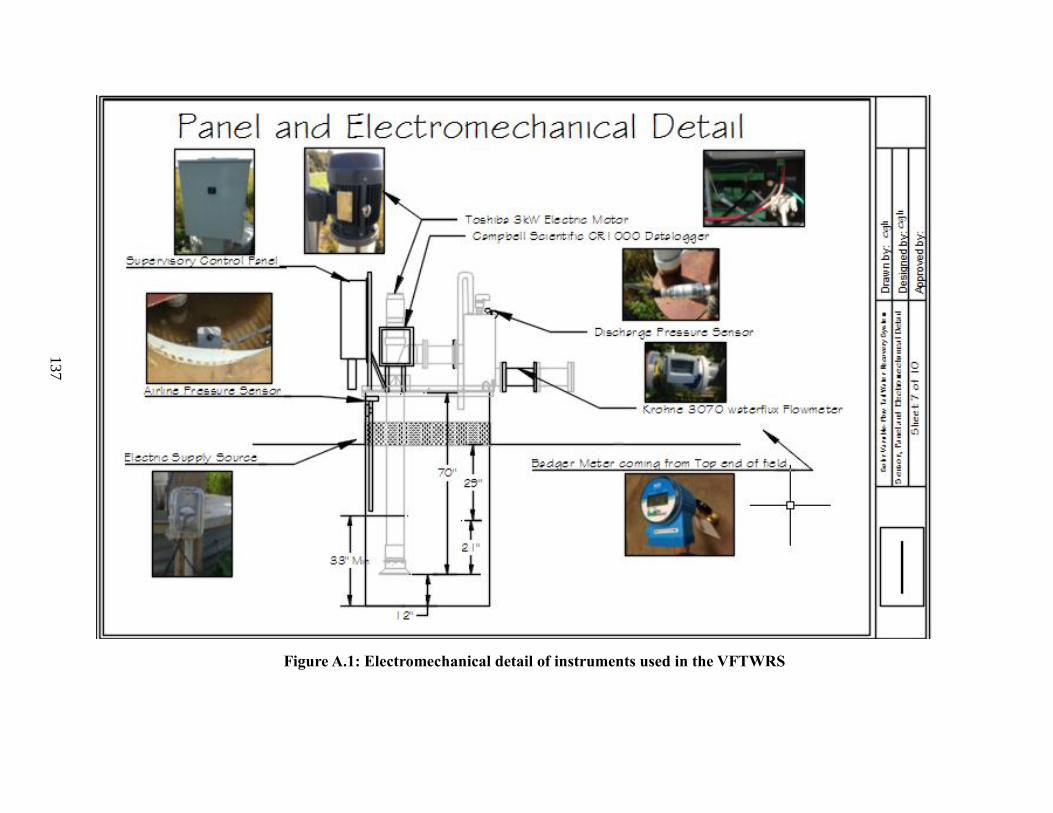
137

Figure A.1: Electromechanical detail of instruments used in the VFTWRS

137

138

Figure A.2: Plan for Scenario 1 (VFTWRS-Grid with lay-flat pipe)

138

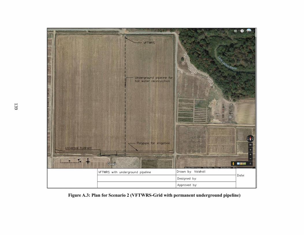
139

Figure A.3: Plan for Scenario 2 (VFTWRS-Grid with permanent underground pipeline)

139

140

Figure A.4: Plan for Scenario 3 (VFTWRS-PV with lay-flat pipe)

140

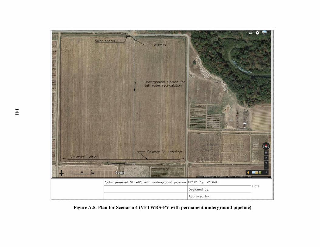
141

Figure A.5: Plan for Scenario 4 (VFTWRS-PV with permanent underground pipeline)

141

142

Figure A.6: Plan for Scenario 5 (Tail-water recovery system with a full sized pit)

142

143

Figure A.7: Plan for Scenario 6 (Tail-water recovery system with a half sized pit)

143

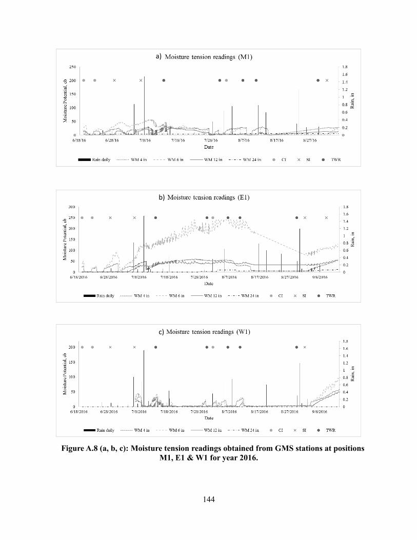
144

Figure A.8 (a, b, c): Moisture tension readings obtained from GMS stations at positions

M1, E1 & W1 for year 2016.

a)

b)

c)

145

Figure A.8 (d, e, f): Moisture tension readings obtained from GMS stations at positions

M2, E2 & W2 for year 2016 (Cont.).

d)

e)

f)

146

Figure A.8 (g, h, i): Moisture tension readings obtained from GMS stations at positions


g)

h)

i)

147

Figure A.8 (j, k, l): Moisture tension readings obtained from GMS stations at positions


j)

k)

l)

148

Figure A.8 (m, n): Moisture tension readings obtained from GMS stations at positions


m)

n)

149

Figure A.9 (a, b, c): Moisture tension readings obtained from GMS stations at positions

M1, E1 & W1 for year 2017.

a)

b)

c)

150

Figure A.9 (d, e, f): Moisture tension readings obtained from GMS stations at positions


d)

e)

f)

151

Figure A.9 (g, h, i): Moisture tension readings obtained from GMS stations at positions


g)

h)

i)

152

Figure A.9 (j, k, l): Moisture tension readings obtained from GMS stations at positions


j)

k)

l)

153

Figure A.9 (m, n): Moisture tension readings obtained from GMS stations at positions


m)

n)