EVALUATION OF ANOMALY AND FAILURE SCENARIOS INVOLVING ANEXPLORATION ROVER: A BAYESIAN NETWORK APPROACH.

Daniele Codetta-Raiteri1, Luigi Portinale1, Andrea Guiotto2, and Yuri Yushtein3

1DiSIT, Computer Science Institute, University of Piemonte Orientale, 15121 Alessandria, Italy2Business Unit Optical Observation & Science Engineering Software, Thales Alenia Space, 10146 Torino, Italy

3Systems, Software & Technology Department, ESA-ESTEC, 2200 Noordwijk, The Netherlands

ABSTRACT

Recent studies focused on the achievement of autonomyby spacecrafts, with the aim of avoiding the interventionof the ground control. In this sense, the ARPHA soft-ware prototype has been developed for the automatic fail-ure detection, identification and recovery (FDIR), and isbased on the on-board analysis of a Dynamic BayesianNetwork (DBN) representing the system behaviour con-ditioned by the conditions of components and environ-ment. In this paper, we describe the main functionali-ties of ARPHA, and we apply its FDIR capabilities tothe power supply subsystem of an exploring rover, takinginto account four scenarios leading to anomalies or fail-ures. The DBN model of the system is described. Then,we test the execution of ARPHA, together with a roversimulator providing sensor data and plan data. In par-ticular, we show the results of diagnosis, prognosis andrecovery, returned by ARPHA when the scenarios occur.

Key words: Failure Detection, Identification and Recov-ery; autonomous systems; dynamic Bayesian networks.

1. INTRODUCTION

Recent studies tried to obtain the autonomy by space-crafts, in order to avoid the involvement of the groundcontrol to solve malfunctioning issues. Several avail-able techniques for system diagnosis and prognosis havebeen considered and evaluated for the application in thespace exploration domain [1, 2, 3]. The traditional ap-proach for on-board FDIR (Fault Detection, Identifica-tion and Recovery) is based on the run-time observationof the system operational status (health monitoring) in or-der to detect faults, while the initiation of the correspond-ing recovery actions uses static pre-compiled look-up ta-bles. In this paper, we present ARPHA (Anomaly Res-olution and Prognostic Health management for Auton-omy), a software prototype for automatic FDIR, based onthe on-board analysis (inference) of a Dynamic BayesianNetworks (DBN) [4] representing the system behaviour.Bayesian Networks (BN) [5] are a typical probabilistic

graphical model allowing the computation of diagnos-tic and predictive measures, possibly conditioned by thepartial observation of the system. DBN is a particularform of BN and introduces a discrete temporal dimen-sion (Sec. 2). The system can be initially modelled as aDynamic Fault Tree (DFT) [6] which is a model familiarto reliability engineers. The DFT can be automaticallytransformed in DBN [7] which can be completed by theuser adding the system features that are not captured bythe DFT model. The enriched DBN (in Junction Tree(JT) [8] form) becomes the on-board model that ARPHAexploits for FDIR conditioned by observations comingfrom the system sensors and concerning the componentsor environment conditions (Sec. 3). In this paper, we ap-ply ARPHA to an exploring rover in specific scenariospossibly leading to anomalies or failures. In particular,we take into account the power supply subsystem, witha specific attention to the power generation by solar ar-rays, the load due to the current action performed by therover, and the variations to the battery charge due to thedifference between the amounts of power generation andload. ARPHA is executed together with a rover simulatorgenerating the observations from the sensors. ARPHAestimates, at each time step, the current system state (Di-agnosis) and the future state (Prognosis), and select themost suitable Recovery policy in case of detection of cur-rent or future anomalies or failures (Sec. 4).

2. BASIC NOTIONS ABOUT DBN

BN [5] are defined by a direct acyclic graph (DAG) whereeach node is a discrete random variable. Each node hasassociated a conditional probability table (CPT) specify-ing the probability of each value of the node, conditionedby every instantiation of parent nodes. In this way, it ispossible to include local conditional dependencies, by di-rectly specifying the causes that influence a given effect.This allows computing the probability distribution of anyvariable given the observation of the values of any subsetof the other variables. DBN extend BN by providing adiscrete temporal dimension. A DBN is essentially thereplication of a BN over two time slices, t − ∆ and t,where ∆ is the time discretization step. If a variable is

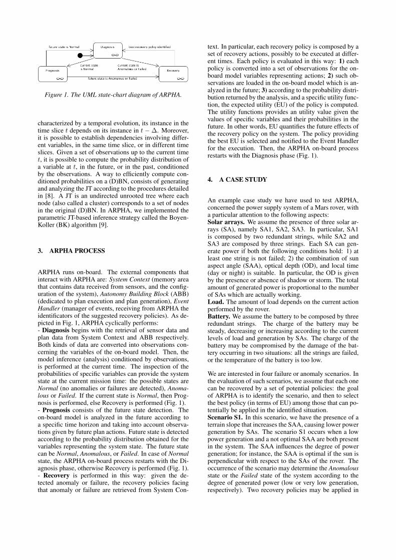
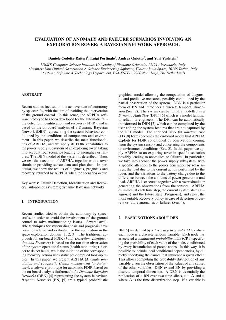
Figure 1. The UML state-chart diagram of ARPHA.

characterized by a temporal evolution, its instance in thetime slice t depends on its instance in t −∆. Moreover,it is possible to establish dependencies involving differ-ent variables, in the same time slice, or in different timeslices. Given a set of observations up to the current timet, it is possible to compute the probability distribution ofa variable at t, in the future, or in the past, conditionedby the observations. A way to efficiently compute con-ditioned probabilities on a (D)BN, consists of generatingand analyzing the JT according to the procedures detailedin [8]. A JT is an undirected unrooted tree where eachnode (also called a cluster) corresponds to a set of nodesin the original (D)BN. In ARPHA, we implemented theparametric JT-based inference strategy called the Boyen-Koller (BK) algorithm [9].

3. ARPHA PROCESS

ARPHA runs on-board. The external components thatinteract with ARPHA are: System Context (memory areathat contains data received from sensors, and the config-uration of the system), Autonomy Building Block (ABB)(dedicated to plan execution and plan generation), EventHandler (manager of events, receiving from ARPHA theidentificators of the suggested recovery policies). As de-picted in Fig. 1, ARPHA cyclically performs:- Diagnosis begins with the retrieval of sensor data andplan data from System Context and ABB respectively.Both kinds of data are converted into observations con-cerning the variables of the on-board model. Then, themodel inference (analysis) conditioned by observations,is performed at the current time. The inspection of theprobabilities of specific variables can provide the systemstate at the current mission time: the possible states areNormal (no anomalies or failures are detected), Anoma-lous or Failed. If the current state is Normal, then Prog-nosis is performed, else Recovery is performed (Fig. 1).- Prognosis consists of the future state detection. Theon-board model is analyzed in the future according toa specific time horizon and taking into account observa-tions given by future plan actions. Future state is detectedaccording to the probability distribution obtained for thevariables representing the system state. The future statecan be Normal, Anomalous, or Failed. In case of Normalstate, the ARPHA on-board process restarts with the Di-agnosis phase, otherwise Recovery is performed (Fig. 1).- Recovery is performed in this way: given the de-tected anomaly or failure, the recovery policies facingthat anomaly or failure are retrieved from System Con-

text. In particular, each recovery policy is composed by aset of recovery actions, possibly to be executed at differ-ent times. Each policy is evaluated in this way: 1) eachpolicy is converted into a set of observations for the on-board model variables representing actions; 2) such ob-servations are loaded in the on-board model which is an-alyzed in the future; 3) according to the probability distri-bution returned by the analysis, and a specific utility func-tion, the expected utility (EU) of the policy is computed.The utility functions provides an utility value given thevalues of specific variables and their probabilities in thefuture. In other words, EU quantifies the future effects ofthe recovery policy on the system. The policy providingthe best EU is selected and notified to the Event Handlerfor the execution. Then, the ARPHA on-board processrestarts with the Diagnosis phase (Fig. 1).

4. A CASE STUDY

An example case study we have used to test ARPHA,concerned the power supply system of a Mars rover, witha particular attention to the following aspects:Solar arrays. We assume the presence of three solar ar-rays (SA), namely SA1, SA2, SA3. In particular, SA1is composed by two redundant strings, while SA2 andSA3 are composed by three strings. Each SA can gen-erate power if both the following conditions hold: 1) atleast one string is not failed; 2) the combination of sunaspect angle (SAA), optical depth (OD), and local time(day or night) is suitable. In particular, the OD is givenby the presence or absence of shadow or storm. The totalamount of generated power is proportional to the numberof SAs which are actually working.Load. The amount of load depends on the current actionperformed by the rover.Battery. We assume the battery to be composed by threeredundant strings. The charge of the battery may besteady, decreasing or increasing according to the currentlevels of load and generation by SAs. The charge of thebattery may be compromised by the damage of the bat-tery occurring in two situations: all the strings are failed,or the temperature of the battery is too low.

We are interested in four failure or anomaly scenarios. Inthe evaluation of such scenarios, we assume that each onecan be recovered by a set of potential policies: the goalof ARPHA is to identify the scenario, and then to selectthe best policy (in terms of EU) among those that can po-tentially be applied in the identified situation.Scenario S1. In this scenario, we have the presence of aterrain slope that increases the SAA, causing lower powergeneration by SAs. The scenario S1 occurs when a lowpower generation and a not optimal SAA are both presentin the system. The SAA influences the degree of powergeneration; for instance, the SAA is optimal if the sun isperpendicular with respect to the SAs of the rover. Theoccurrence of the scenario may determine the Anomalousstate or the Failed state of the system according to thedegree of generated power (low or very low generation,respectively). Two recovery policies may be applied in

case of detection of S1, with the aim of reducing the neg-ative effects: P1) transition to stand-by mode includingthe suspension of the plan, with the aim of reducing theload while the power generation is limited. P2) change ofinclination of SA2 and SA3, with the goal of improvingthe SAA and consequently the level of power generation(the tilting system cannot act on SA1).Scenario S2. In this scenario, we have the presence ofdust or shadow that increases the OD and reduces thepower generated by SAs. The scenario S2 occurs whenboth a low power generation and a compromised OD arepresent in the system. The presence of dust in the air orthe rover positioned in a shadowed area, reduce the irra-diation of SAs, and the degree of generated power, as aconsequence. In the best situation, there is no dust and theOD is null. The OD grows proportionally to the densityof dust in the air, or the level of obscurity. The occur-rence of S2 determines the Anomalous state or the Failedstate, given the level of power generation. Two recoverypolicies may be applied to face S2 and improve the situa-tion: P3) movement of the rover into another position, inorder to try to avoid the dust or the shadow, and improvethe power generation as a consequence. P4) modifica-tion of the inclination of SA2 and SA3 (to compensatefor the OD, with a better SAA), retraction of the drill ifa drilling operation is under execution (safe condition forthe drilling device), and transition to stand-by mode (toreduce the load).Scenario S3. In this scenario, we have an unexpectedhigh request of energy by the drilling operation. Thepower generated by SAs may not be enough to copewith the request of energy, so the battery may be usedto provide the additional power. The scenario S3 occurswhen the level of battery charge is not optimal during thedrilling operation. This leads the system to the Anoma-lous or Failed state according to degree of charge of thebattery. The recovery policies facing S3 are the follow-ing: P4) as above; the goal is improving the power gen-eration thanks to a better SAA, and avoiding the use ofthe battery by suspending the drill. P5) suspension of theplan, retraction of the drill if drilling is under execution,and transition to stand-by mode (with the aim of reducingthe load).Scenario S4. If the battery is damaged, the battery chargelevel may become low. The scenario S4 occurs when boththe battery damage and the low battery charge character-ize the system. The damage may be due to the low tem-perature of the battery or the failure of its strings. In thiscase, we have a damage due to a low external temper-ature; such a fault is transient, since an increase of thetemperature can bring back the battery to work correctly.The Anomalous or Failed state depends on the degree ofcharge. The recovery policies considered for S4 are P2and P4 defined as above. In this case, the aim of the poli-cies is to suspend the plan and then to try to get powerfrom a better inclination of SAs. Notice that P2 and P4are potentially different (even when a drilling operationis not involved), since P2 first stops the current plan andthen moves the SAs, while P4 tries to move SAs beforestopping the plan.

4.1. The DBN model of the case study

The DBN model (Fig. 2.a) of the case study has the fol-lowing features:Solar arrays. The variables representing the function-ing or failure of basic components or subsystems, arebinary; for example, StringSA11 and StringSA12 repre-sent the state of a string of SA1, while StringsSA1 repre-sents the state of the set of strings. The variables model-ing environmental conditions are binary, in order to rep-resent the presence or absence of such conditions; thisis the case of the variables Storm and Shadow influenc-ing OpticalDepth, and the variable Time (day or night).The variable AngleSA1 representing the SAA of SA1, isternary (good, discrete, bad). The fact that the combi-nation of OpticalDepth, Time, AngleSA1 allows or com-promises the power generation by SA1, is represented bythe binary variable SA1perf. Such variable, together withStringsSA1, influences the binary variable PowGenSA1modelling the presence or absence of power generationby SA1. SA2 and SA3 are modelled in the same way.The variable PowGen is influenced by PowGenSA1, Pow-GenSA2, PowGenSA3. The size of PowGen is 4, in orderto represent 4 intermediate levels of power generation de-pending on the number of SAs generating power.Load. The size of the variable ActionId is 8, in order torepresent 8 actions of interest in the model (in this exam-ple, actions may concern either the plan or the recovery).Such variable influences Load whose size is 5, in order torepresent 5 intermediate levels of power consumption ac-cording to the action under execution. The variable Bal-ance is ternary and indicates that PowGen is equal, higheror lower than Load.Battery. The state (working or failed) of each re-dundant string composing the battery is represented byBattString1, BattString2, BattString3, while the state ofthe set of strings is modelled by BattStrings. The vari-able Temp is ternary and represents the temperature of thebattery (low, medium, high). Temp and BattStrings influ-ence BattFail representing the damage of the battery. Thevariable Trend indicates that the battery charge is steady,increasing or decreasing, according to Balance and Bat-tFail. Four intermediate levels of battery charge are rep-resented by the variable BattCharge.Scenarios. The variables S1, S2, S3, S4 are ternary, in or-der to represent the states Normal, Anomalous and Failedin each scenario (the Normal state indicates that the sce-nario does not currently occur).

In the DBN in Fig. 2.a, the instance of a variable at timeslice t is distinguished from the instance at time slicet − ∆, by the symbol # following the name of the vari-able. For instance, StringSA11 is present in t−∆, whileStringSA11# is present in t. If a variable has a temporalevolution its two instances are connected by a temporalarc (appearing as a thick line in Fig. 2.a). Still in Fig. 2.a,the observable variables appear as black nodes; the val-ues coming from sensors, ABB, and recovery policies,will become observations for such variables. In Fig. 2.b,we provide the utility function (on a [0, 1] scale) neces-sary to compare the recovery policies in case of failure or

Figure 2. a) DBN model of the case study. b) Utility function for policies.

anomaly detection due to power supply problems. In par-ticular, the utility function provides an utility value de-pending on the plan or recovery action under executionand the balance between power generation and load. No-tice that there are actions (“standby” and “retract” of thedrill) that, when used in recovery policies, are meant toavoid the rover halting in an unsafe condition (for exam-ple with the drill locked on the ground, with the dangerof icing during the night); such actions have a large util-ity for cases corresponding to low power supply situa-tions (meaning that they are useful for recovering situ-ations where the generated power is less than the load),while they have a small utility in case the power supplyis sufficient to cover the required load. Remaining ac-tions (which are also usual standard plan operations of therover) have a smaller utility in correspondence to casesrelated to low power supply situations, since in such casesone should avoid power consuming actions.

4.2. Executing ARPHA

In order to perform an empirical evaluation of the ap-proach, ARPHA has been deployed in an evaluation plat-form composed by a workstation linked to a PC via Eth-ernet cable. A rover simulator (called ROSEX) has beeninstalled on the workstation. On the PC we installed theTSIM environment, emulating the on-board computinghardware environment (LEON3), and ARPHA runningas a task of RTEMS. Sensors data and plan data that thesimulator provides, are the following: OD, power gener-ated by each SA, SAA of SA1, SA2, SA3, charge andtemperature of the battery, mission elapsed time, actionunder execution, plan under execution.

At each mission step (in DBN, time is discretized), thecurrent sensor data and plan action are retrieved and con-verted into current or future observations for the vari-ables in the on-board model. Such observations are ex-pressed as the probability distribution of the possible vari-able values. For example, in Fig. 3.c, the “wait” (an-other name for “standby”) action in the plan at the mis-sion step 3, is converted in the probability distribution1, 0, 0, 0, 0, 0, 0, 0 concerning the variable ActionId in thesame step. The first value of the distribution indicatesthat the first possible value of the variable (0) has beenobserved with probability 1. This is due to the fact thatActionId represents in the model the plan action (or therecovery action). In particular, the value 0 correspondsto the “wait” action. An example about sensor data isthe sensor pwrsa1 providing the value 15.71248 at themission step 3 (see Fig. 3.c). This value becomes theprobability distribution 1, 0 for the values of the variablePowGenSA1. In other words, PowGenSA1 is observedequal to 0 with probability 1 at the same time step, inorder to represent that SA1 is generating enough power(pwrsa1 > 15) in that step (the value 1 instead, repre-sents that the generated power is too low). We assumethat the power is high if greater than 15 in the case ofSA1, and greater than 25 in the case of SA2 and SA3(SA1 is composed by two strings, while SA2 and SA3

are composed by three strings).

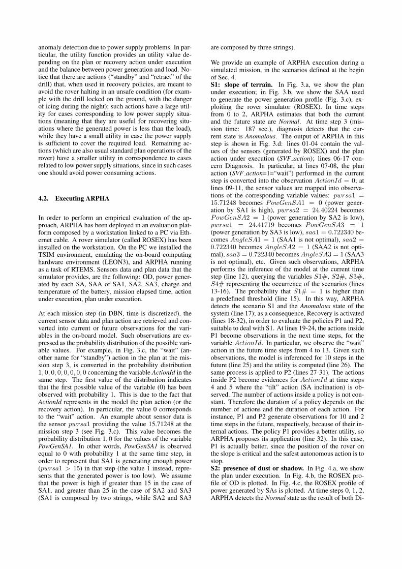
We provide an example of ARPHA execution during asimulated mission, in the scenarios defined at the beginof Sec. 4.S1: slope of terrain. In Fig. 3.a, we show the planunder execution; in Fig. 3.b, we show the SAA usedto generate the power generation profile (Fig. 3.c), ex-ploiting the rover simulator (ROSEX). In time stepsfrom 0 to 2, ARPHA estimates that both the currentand the future state are Normal. At time step 3 (mis-sion time: 187 sec.), diagnosis detects that the cur-rent state is Anomalous. The output of ARPHA in thisstep is shown in Fig. 3.d: lines 01-04 contain the val-ues of the sensors (generated by ROSEX) and the planaction under execution (SVF action); lines 06-17 con-cern Diagnosis. In particular, at lines 07-08, the planaction (SVF action=1=“wait”) performed in the currentstep is converted into the observation ActionId = 0; atlines 09-11, the sensor values are mapped into observa-tions of the corresponding variable values: pwrsa1 =15.71248 becomes PowGenSA1 = 0 (power gener-ation by SA1 is high), pwrsa2 = 24.40224 becomesPowGenSA2 = 1 (power generation by SA2 is low),pwrsa1 = 24.41719 becomes PowGenSA3 = 1(power generation by SA3 is low), saa1 = 0.722340 be-comes AngleSA1 = 1 (SAA1 is not optimal), saa2 =0.722340 becomes AngleSA2 = 1 (SAA2 is not opti-mal), saa3 = 0.722340 becomes AngleSA3 = 1 (SAA3is not optimal), etc. Given such observations, ARPHAperforms the inference of the model at the current timestep (line 12), querying the variables S1#, S2#, S3#,S4# representing the occurrence of the scenarios (lines13-16). The probability that S1# = 1 is higher thana predefined threshold (line 15). In this way, ARPHAdetects the scenario S1 and the Anomalous state of thesystem (line 17); as a consequence, Recovery is activated(lines 18-32), in order to evaluate the policies P1 and P2,suitable to deal with S1. At lines 19-24, the actions insideP1 become observations in the next time steps, for thevariable ActionId. In particular, we observe the “wait”action in the future time steps from 4 to 13. Given suchobservations, the model is inferenced for 10 steps in thefuture (line 25) and the utility is computed (line 26). Thesame process is applied to P2 (lines 27-31). The actionsinside P2 become evidences for ActionId at time steps4 and 5 where the “tilt” action (SA inclination) is ob-served. The number of actions inside a policy is not con-stant. Therefore the duration of a policy depends on thenumber of actions and the duration of each action. Forinstance, P1 and P2 generate observations for 10 and 2time steps in the future, respectively, because of their in-ternal actions. The policy P1 provides a better utility, soARPHA proposes its application (line 32). In this case,P1 is actually better, since the position of the rover onthe slope is critical and the safest autonomous action is tostop.S2: presence of dust or shadow. In Fig. 4.a, we showthe plan under execution. In Fig. 4.b, the ROSEX pro-file of OD is plotted. In Fig. 4.c, the ROSEX profile ofpower generated by SAs is plotted. At time steps 0, 1, 2,ARPHA detects the Normal state as the result of both Di-

d) ARPHA output:00 *** MISSION STEP: 3 (MISSION TIME: 187 sec.) ***01 *************** ROSEX VALUES ***************02 opticaldepht = 1.00000 pwrsa1 = 15.71248 pwrsa2 = 24.40224 pwrsa3 = 24.4171903 saa1 = 0.72340 saa2 = 0.72340 saa3 = 0.72340 batterycharge = 90.2453304 batttemp = 273.00000 time = 10.04274 SVF_action = 1 SVF_plan = 105 *********************************************06 *** Diagnosis ***07 Propagate PLAN STREAM08 3:ActionId#:1 0 0 0 0 0 0 0 :09 Propagate SENSORS STREAM10 3:OpticalDepth#:1 0 : 3:PowGenSA1#:1 0 : 3:PowGenSA2#:0 1 : 3:PowGenSA3#:0 1 : 3:AngleSA1#:0 1 0:11 3:AngleSA2#:0 1 0 : 3:AngleSA3#:0 1 0 : 3:BattCharge#:0 0 0 1 : 3:Temp#:0 1 0 : 3:Time#:1 0 :12 Current inference (STEP 3)13 Pr{S1#=2} = 0.00000000 < 0.99000000 Pr{S2#=2} = 0.00000000 < 0.5900000014 Pr{S3#=2} = 0.00000000 < 0.99000000 Pr{S4#=2} = 0.00000000 < 0.9900000015 Pr{S1#=1} = 1.00000000 >= 0.99000000 Pr{S2#=1} excluded because under recovery or minor criticality16 Pr{S3#=1} = 0.00000000 < 0.99000000 Pr{S4#=1} = 0.00000000 < 0.9900000017 SYSTEM STATE: "ANOMALOUS" (S1#=1)18 ## Preventive Recovery ##19 Policy to convert: P120 Propagate POLICY STREAM21 4:ActionId#:1 0 0 0 0 0 0 0 : 5:ActionId#:1 0 0 0 0 0 0 0 : 6:ActionId#:1 0 0 0 0 0 0 0 :22 7:ActionId#:1 0 0 0 0 0 0 0 : 8:ActionId#:1 0 0 0 0 0 0 0 : 9:ActionId#:1 0 0 0 0 0 0 0 :23 10:ActionId#:1 0 0 0 0 0 0 0 : 11:ActionId#:1 0 0 0 0 0 0 0 : 12:ActionId#:1 0 0 0 0 0 0 0 :24 13:ActionId#:1 0 0 0 0 0 0 0 :25 Future inference (STEP 13)26 Utility Function= 0.473627 Policy to convert: P228 Propagate POLICY STREAM29 4:ActionId#:0 0 0 0 0 0 1 0 : 5:ActionId#:0 0 0 0 0 0 1 0 :30 Future inference (STEP 13)31 Utility Function= 0.062232 Best policy for Preventive Recovery is P1

Figure 3. Scenario S1: a) plan under execution. b) Sun Aspect Angle (SAA) of solar array SA2. c) Power generation bysolar arrays SA1, SA2, SA3. d) ARPHA output at time step 3 (mission time: 187 sec.).

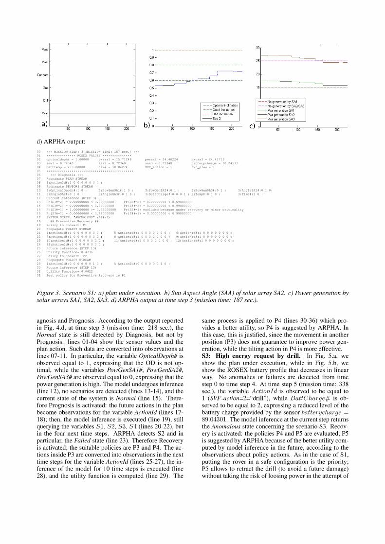
agnosis and Prognosis. According to the output reportedin Fig. 4.d, at time step 3 (mission time: 218 sec.), theNormal state is still detected by Diagnosis, but not byPrognosis: lines 01-04 show the sensor values and theplan action. Such data are converted into observations atlines 07-11. In particular, the variable OpticalDepth# isobserved equal to 1, expressing that the OD is not op-timal, while the variables PowGenSA1#, PowGenSA2#,PowGenSA3# are observed equal to 0, expressing that thepower generation is high. The model undergoes inference(line 12), no scenarios are detected (lines 13-14), and thecurrent state of the system is Normal (line 15). There-fore Prognosis is activated: the future actions in the planbecome observations for the variable ActionId (lines 17-18); then, the model inference is executed (line 19), stillquerying the variables S1, S2, S3, S4 (lines 20-22), butin the four next time steps. ARPHA detects S2 and inparticular, the Failed state (line 23). Therefore Recoveryis activated; the suitable policies are P3 and P4. The ac-tions inside P3 are converted into observations in the nexttime steps for the variable ActionId (lines 25-27), the in-ference of the model for 10 time steps is executed (line28), and the utility function is computed (line 29). The

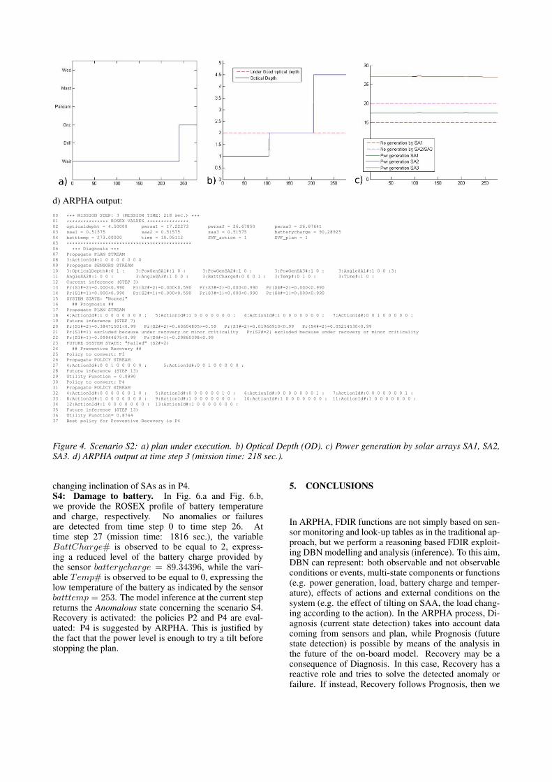
same process is applied to P4 (lines 30-36) which pro-vides a better utility, so P4 is suggested by ARPHA. Inthis case, this is justified, since the movement in anotherposition (P3) does not guarantee to improve power gen-eration, while the tilting action in P4 is more effective.S3: High energy request by drill. In Fig. 5.a, weshow the plan under execution, while in Fig. 5.b, weshow the ROSEX battery profile that decreases in linearway. No anomalies or failures are detected from timestep 0 to time step 4. At time step 5 (mission time: 338sec.), the variable ActionId is observed to be equal to1 (SVF action=2=“drill”), while BattCharge# is ob-served to be equal to 2, expressing a reduced level of thebattery charge provided by the sensor batterycharge =89.04301. The model inference at the current step returnsthe Anomalous state concerning the scenario S3. Recov-ery is activated: the policies P4 and P5 are evaluated; P5is suggested by ARPHA because of the better utility com-puted by model inference in the future, according to theobservations about policy actions. As in the case of S1,putting the rover in a safe configuration is the priority;P5 allows to retract the drill (to avoid a future damage)without taking the risk of loosing power in the attempt of

d) ARPHA output:00 *** MISSION STEP: 3 (MISSION TIME: 218 sec.) ***01 *************** ROSEX VALUES ***************02 opticaldepht = 4.50000 pwrsa1 = 17.22273 pwrsa2 = 26.67850 pwrsa3 = 26.6764103 saa1 = 0.51575 saa2 = 0.51575 saa3 = 0.51575 batterycharge = 90.2892504 batttemp = 273.00000 time = 10.05112 SVF_action = 1 SVF_plan = 105 *********************************************06 *** Diagnosis ***07 Propagate PLAN STREAM08 3:ActionId#:1 0 0 0 0 0 0 009 Propagate SENSORS STREAM10 3:OpticalDepth#:0 1 : 3:PowGenSA1#:1 0 : 3:PowGenSA2#:1 0 : 3:PowGenSA3#:1 0 : 3:AngleSA1#:1 0 0 :3:11 AngleSA2#:1 0 0 : 3:AngleSA3#:1 0 0 : 3:BattCharge#:0 0 0 1 : 3:Temp#:0 1 0 : 3:Time#:1 0 :12 Current inference (STEP 3)13 Pr{S1#=2}=0.000<0.990 Pr{S2#=2}=0.000<0.590 Pr{S3#=2}=0.000<0.990 Pr{S4#=2}=0.000<0.99014 Pr{S1#=1}=0.000<0.990 Pr{S2#=1}=0.000<0.590 Pr{S3#=1}=0.000<0.990 Pr{S4#=1}=0.000<0.99015 SYSTEM STATE: "Normal"16 ## Prognosis ##17 Propagate PLAN STREAM18 4:ActionId#:1 0 0 0 0 0 0 0 : 5:ActionId#:1 0 0 0 0 0 0 0 : 6:ActionId#:1 0 0 0 0 0 0 0 : 7:ActionId#:0 0 1 0 0 0 0 0 :19 Future inference (STEP 7)20 Pr{S1#=2}=0.38471501<0.99 Pr{S2#=2}=0.60604805>=0.59 Pr{S3#=2}=0.01966910<0.99 Pr{S4#=2}=0.05214530<0.9921 Pr{S1#=1} excluded because under recovery or minor criticality Pr{S2#=2} excluded because under recovery or minor criticality22 Pr{S3#=1}=0.09944675<0.99 Pr{S4#=1}=0.29860398<0.9923 FUTURE SYSTEM STATE: "Failed" (S2#=2)24 ## Preventive Recovery ##25 Policy to convert: P326 Propagate POLICY STREAM27 4:ActionId#:0 0 1 0 0 0 0 0 : 5:ActionId#:0 0 1 0 0 0 0 0 :28 Future inference (STEP 13)29 Utility Function = 0.089030 Policy to convert: P431 Propagate POLICY STREAM32 4:ActionId#:0 0 0 0 0 0 1 0 : 5:ActionId#:0 0 0 0 0 0 1 0 : 6:ActionId#:0 0 0 0 0 0 0 1 : 7:ActionId#:0 0 0 0 0 0 0 1 :33 8:ActionId#:1 0 0 0 0 0 0 0 : 9:ActionId#:1 0 0 0 0 0 0 0 : 10:ActionId#:1 0 0 0 0 0 0 0 : 11:ActionId#:1 0 0 0 0 0 0 0 :34 12:ActionId#:1 0 0 0 0 0 0 0 : 13:ActionId#:1 0 0 0 0 0 0 0 :35 Future inference (STEP 13)36 Utility Function= 0.876437 Best policy for Preventive Recovery is P4

Figure 4. Scenario S2: a) plan under execution. b) Optical Depth (OD). c) Power generation by solar arrays SA1, SA2,SA3. d) ARPHA output at time step 3 (mission time: 218 sec.).

changing inclination of SAs as in P4.S4: Damage to battery. In Fig. 6.a and Fig. 6.b,we provide the ROSEX profile of battery temperatureand charge, respectively. No anomalies or failuresare detected from time step 0 to time step 26. Attime step 27 (mission time: 1816 sec.), the variableBattCharge# is observed to be equal to 2, express-ing a reduced level of the battery charge provided bythe sensor batterycharge = 89.34396, while the vari-able Temp# is observed to be equal to 0, expressing thelow temperature of the battery as indicated by the sensorbatttemp = 253. The model inference at the current stepreturns the Anomalous state concerning the scenario S4.Recovery is activated: the policies P2 and P4 are eval-uated: P4 is suggested by ARPHA. This is justified bythe fact that the power level is enough to try a tilt beforestopping the plan.

5. CONCLUSIONS

In ARPHA, FDIR functions are not simply based on sen-sor monitoring and look-up tables as in the traditional ap-proach, but we perform a reasoning based FDIR exploit-ing DBN modelling and analysis (inference). To this aim,DBN can represent: both observable and not observableconditions or events, multi-state components or functions(e.g. power generation, load, battery charge and temper-ature), effects of actions and external conditions on thesystem (e.g. the effect of tilting on SAA, the load chang-ing according to the action). In the ARPHA process, Di-agnosis (current state detection) takes into account datacoming from sensors and plan, while Prognosis (futurestate detection) is possible by means of the analysis inthe future of the on-board model. Recovery may be aconsequence of Diagnosis. In this case, Recovery has areactive role and tries to solve the detected anomaly orfailure. If instead, Recovery follows Prognosis, then we

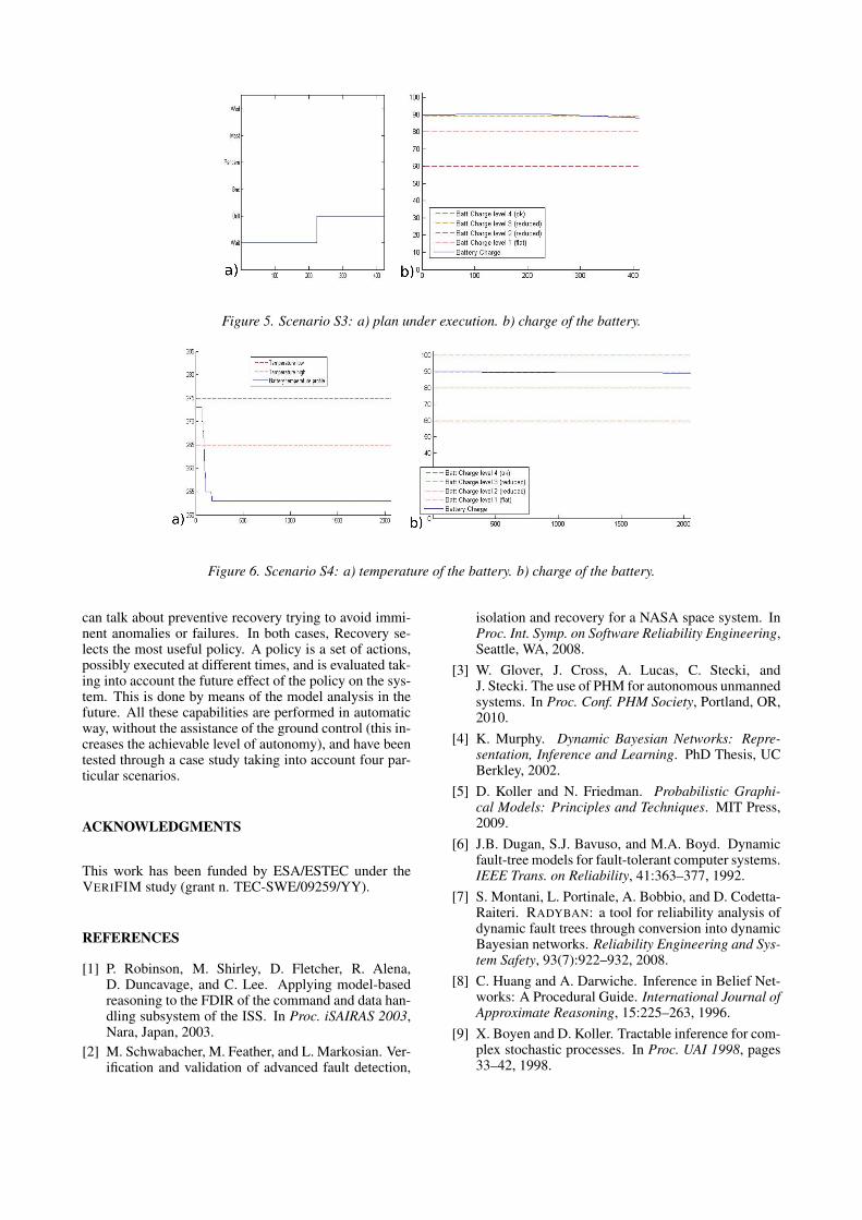
Figure 5. Scenario S3: a) plan under execution. b) charge of the battery.

Figure 6. Scenario S4: a) temperature of the battery. b) charge of the battery.

can talk about preventive recovery trying to avoid immi-nent anomalies or failures. In both cases, Recovery se-lects the most useful policy. A policy is a set of actions,possibly executed at different times, and is evaluated tak-ing into account the future effect of the policy on the sys-tem. This is done by means of the model analysis in thefuture. All these capabilities are performed in automaticway, without the assistance of the ground control (this in-creases the achievable level of autonomy), and have beentested through a case study taking into account four par-ticular scenarios.

ACKNOWLEDGMENTS

This work has been funded by ESA/ESTEC under theVERIFIM study (grant n. TEC-SWE/09259/YY).

REFERENCES

[1] P. Robinson, M. Shirley, D. Fletcher, R. Alena,D. Duncavage, and C. Lee. Applying model-basedreasoning to the FDIR of the command and data han-dling subsystem of the ISS. In Proc. iSAIRAS 2003,Nara, Japan, 2003.

[2] M. Schwabacher, M. Feather, and L. Markosian. Ver-ification and validation of advanced fault detection,

isolation and recovery for a NASA space system. InProc. Int. Symp. on Software Reliability Engineering,Seattle, WA, 2008.

[3] W. Glover, J. Cross, A. Lucas, C. Stecki, andJ. Stecki. The use of PHM for autonomous unmannedsystems. In Proc. Conf. PHM Society, Portland, OR,2010.

[4] K. Murphy. Dynamic Bayesian Networks: Repre-sentation, Inference and Learning. PhD Thesis, UCBerkley, 2002.

[5] D. Koller and N. Friedman. Probabilistic Graphi-cal Models: Principles and Techniques. MIT Press,2009.

[6] J.B. Dugan, S.J. Bavuso, and M.A. Boyd. Dynamicfault-tree models for fault-tolerant computer systems.IEEE Trans. on Reliability, 41:363–377, 1992.

[7] S. Montani, L. Portinale, A. Bobbio, and D. Codetta-Raiteri. RADYBAN: a tool for reliability analysis ofdynamic fault trees through conversion into dynamicBayesian networks. Reliability Engineering and Sys-tem Safety, 93(7):922–932, 2008.

[8] C. Huang and A. Darwiche. Inference in Belief Net-works: A Procedural Guide. International Journal ofApproximate Reasoning, 15:225–263, 1996.

[9] X. Boyen and D. Koller. Tractable inference for com-plex stochastic processes. In Proc. UAI 1998, pages33–42, 1998.