Evaluation of cloudiness simulated by climate models using CALIPSO and PARASOL

H. Chepfer

Laboratoire Météorologie Dynamique / Institut Pierre Simon Laplace,

France

Contributors : S. Bony, G. Cesana, JL Dufresne, D. Konsta, LMD/IPSL

D. Winker, NASA/LaRCD. Tanré, LOAC. Nam, MPI

Y. Zhang, S. Klein, LLNLJ. Cole, U. Toronto

A. Bodas-Salcedo, UKMO

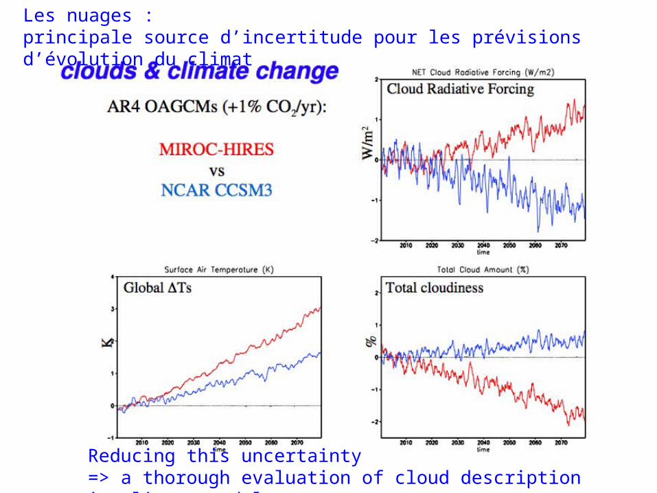
Les nuages : principale source d’incertitude pour les prévisions d’évolution du climat

Reducing this uncertainty => a thorough evaluation of cloud description in climate models

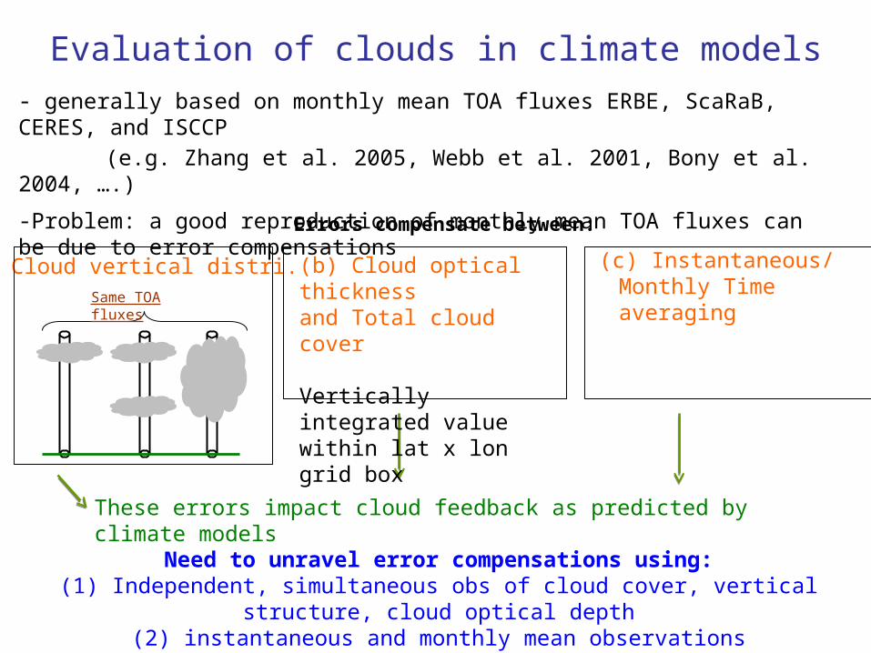
Evaluation of clouds in climate models- generally based on monthly mean TOA fluxes ERBE, ScaRaB, CERES, and ISCCP

(e.g. Zhang et al. 2005, Webb et al. 2001, Bony et al. 2004, ….)

-Problem: a good reproduction of monthly mean TOA fluxes can be due to error compensations

Same TOA fluxes

These errors impact cloud feedback as predicted by climate models

Errors compensate between:

Need to unravel error compensations using:(1) Independent, simultaneous obs of cloud cover, vertical structure, cloud optical depth

(2) instantaneous and monthly mean observations(3) methods for consistent model/obs comparisons

(a) Cloud vertical distri. (c) Instantaneous/ Monthly Time averaging

(b) Cloud optical thicknessand Total cloud cover

Vertically integrated valuewithin lat x lon grid box

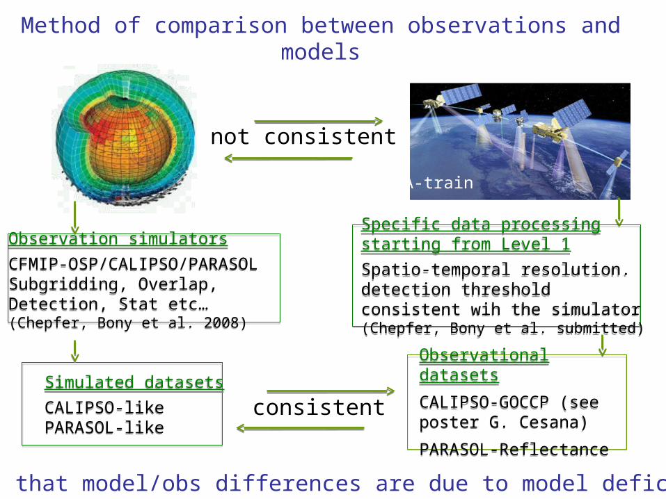
A-train

Observation simulators

CFMIP-OSP/CALIPSO/PARASOLSubgridding, Overlap, Detection, Stat etc… (Chepfer, Bony et al. 2008)

Observation simulators

CFMIP-OSP/CALIPSO/PARASOLSubgridding, Overlap, Detection, Stat etc… (Chepfer, Bony et al. 2008)

Observational datasets

CALIPSO-GOCCP (see poster G. Cesana)

PARASOL-Reflectance

Observational datasets

CALIPSO-GOCCP (see poster G. Cesana)

PARASOL-Reflectance

not consistent

Method of comparison between observations and models

consistentSimulated datasets

CALIPSO-likePARASOL-like

Simulated datasets

CALIPSO-likePARASOL-like

Specific data processing starting from Level 1

Spatio-temporal resolution. detection threshold consistent wih the simulator (Chepfer, Bony et al. submitted)

Specific data processing starting from Level 1

Spatio-temporal resolution. detection threshold consistent wih the simulator (Chepfer, Bony et al. submitted)

Ensures that model/obs differences are due to model deficiencies

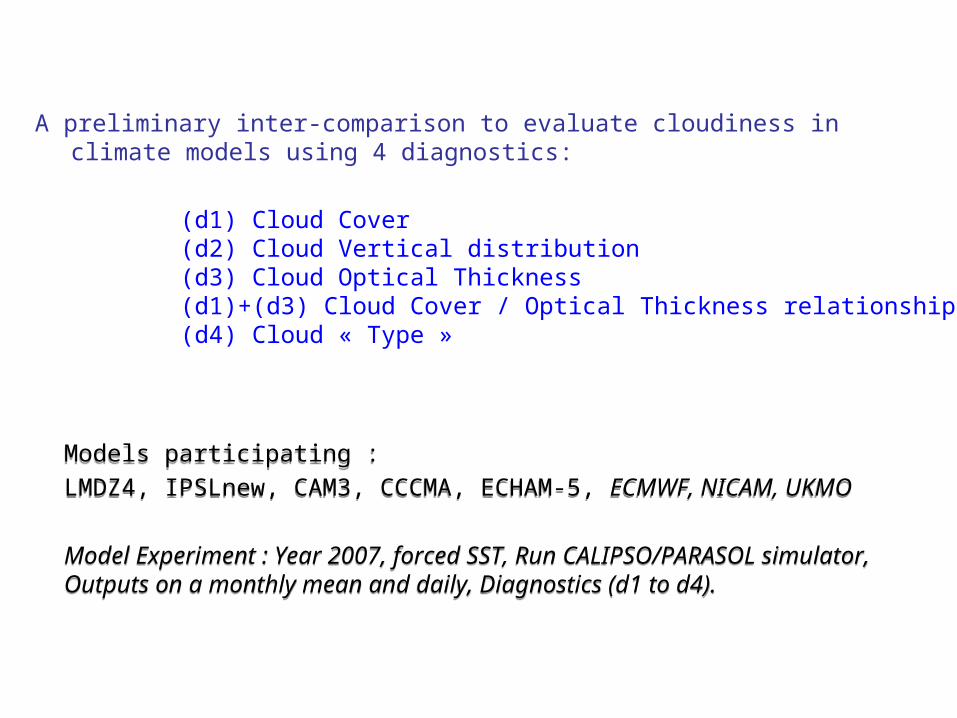
Models participating :

LMDZ4, IPSLnew, CAM3, CCCMA, ECHAM-5, ECMWF, NICAM, UKMO

Model Experiment : Year 2007, forced SST, Run CALIPSO/PARASOL simulator, Outputs on a monthly mean and daily, Diagnostics (d1 to d4).

Models participating :

LMDZ4, IPSLnew, CAM3, CCCMA, ECHAM-5, ECMWF, NICAM, UKMO

Model Experiment : Year 2007, forced SST, Run CALIPSO/PARASOL simulator, Outputs on a monthly mean and daily, Diagnostics (d1 to d4).

A preliminary inter-comparison to evaluate cloudiness in climate models using 4 diagnostics:

(d1) Cloud Cover (d2) Cloud Vertical distribution (d3) Cloud Optical Thickness (d1)+(d3) Cloud Cover / Optical Thickness relationship(d4) Cloud « Type »

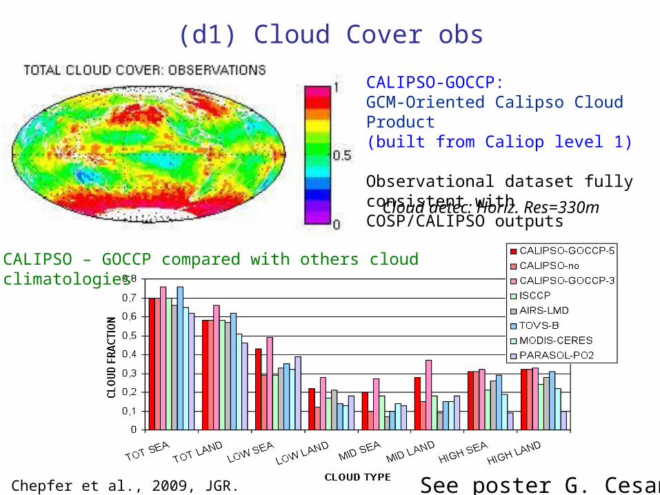
(d1) Cloud Cover obs

CALIPSO-GOCCP:GCM-Oriented Calipso Cloud Product(built from Caliop level 1)

Observational dataset fully consistent with COSP/CALIPSO outputs

CALIPSO – GOCCP compared with others cloud climatologies

Chepfer et al., 2009, JGR. submitted

Cloud detec: Horiz. Res=330m

See poster G. Cesana

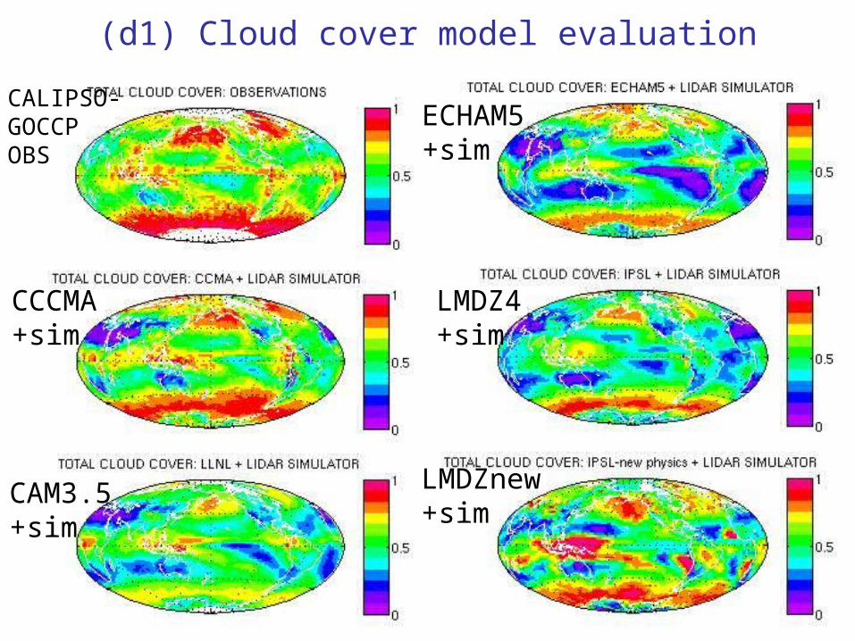
(d1) Cloud cover model evaluation

CALIPSO-GOCCPOBS

CCCMA+sim

CAM3.5+sim

ECHAM5+sim

LMDZ4+sim

LMDZnew+sim

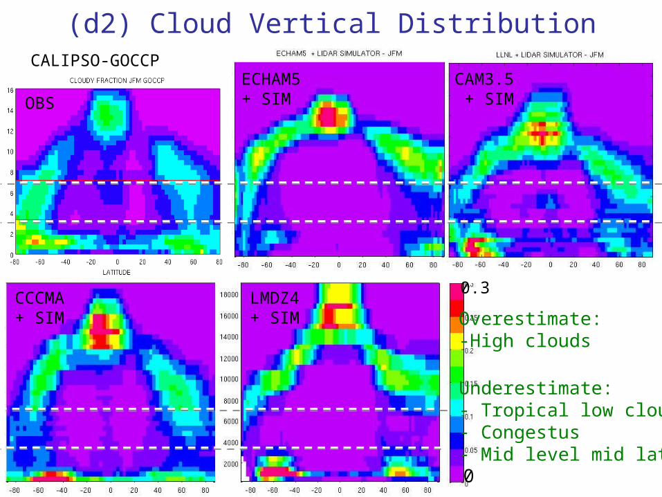
(d2) Cloud Vertical Distribution

LMDZ4+ SIM

CCCMA+ SIM

CALIPSO-GOCCPCAM3.5 + SIM

ECHAM5 + SIM

Overestimate:-High clouds

Underestimate:- Tropical low clouds- Congestus- Mid level mid lat

OBS

0

0.3

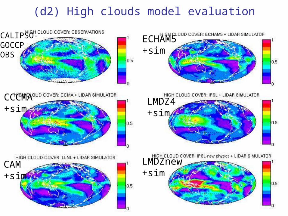
(d2) High clouds model evaluation

CCCMA+sim

CAM+sim

ECHAM5+sim

LMDZ4+sim

LMDZnew+sim

CALIPSO-GOCCPOBS

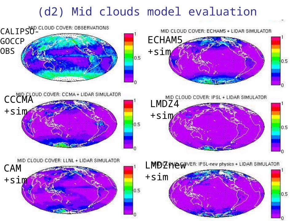
(d2) Mid clouds model evaluation

CCCMA+sim

CAM+sim

ECHAM5+sim

LMDZ4+sim

LMDZnew+sim

CALIPSO-GOCCPOBS

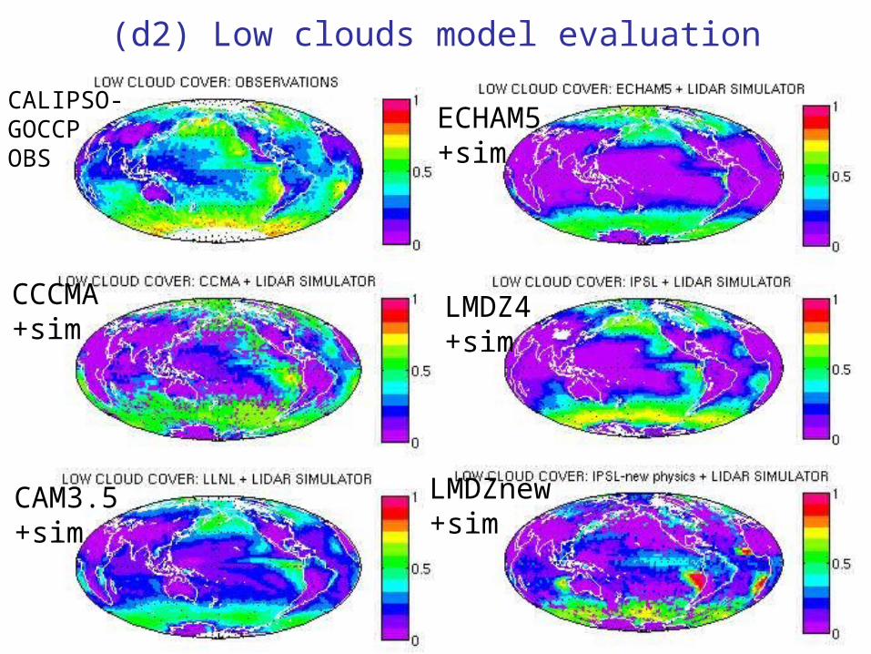
(d2) Low clouds model evaluation

CCCMA+sim

CAM3.5+sim

ECHAM5+sim

LMDZ4+sim

LMDZnew+sim

CALIPSO-GOCCPOBS

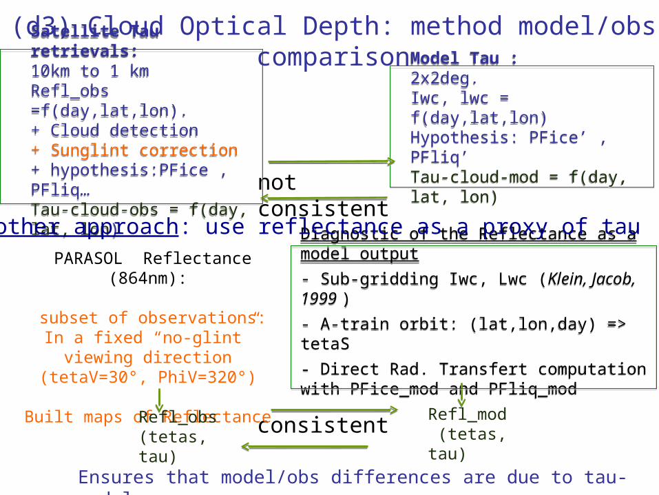
Model Tau : 2x2deg.Iwc, lwc = f(day,lat,lon)Hypothesis: PFice’ , PFliq’Tau-cloud-mod = f(day, lat, lon)

Model Tau : 2x2deg.Iwc, lwc = f(day,lat,lon)Hypothesis: PFice’ , PFliq’Tau-cloud-mod = f(day, lat, lon)

not consistent

consistent

Diagnostic of the Reflectance as a model output

- Sub-gridding Iwc, Lwc (Klein, Jacob, 1999 )

- A-train orbit: (lat,lon,day) => tetaS

- Direct Rad. Transfert computation with PFice_mod and PFliq_mod

Diagnostic of the Reflectance as a model output

- Sub-gridding Iwc, Lwc (Klein, Jacob, 1999 )

- A-train orbit: (lat,lon,day) => tetaS

- Direct Rad. Transfert computation with PFice_mod and PFliq_mod

Satellite Tau retrievals: 10km to 1 kmRefl_obs =f(day,lat,lon).+ Cloud detection+ Sunglint correction+ hypothesis:PFice , PFliq…Tau-cloud-obs = f(day, lat, lon)

Satellite Tau retrievals: 10km to 1 kmRefl_obs =f(day,lat,lon).+ Cloud detection+ Sunglint correction+ hypothesis:PFice , PFliq…Tau-cloud-obs = f(day, lat, lon)

(d3) Cloud Optical Depth: method model/obs comparison

PARASOL Reflectance (864nm):

subset of observations:In a fixed “no-glint” viewing direction

(tetaV=30°, PhiV=320°)

Built maps of Reflectance

Refl_mod (tetas, tau)

Refl_obs(tetas, tau)

Another approach: use reflectance as a proxy of tau

Ensures that model/obs differences are due to tau-model

14

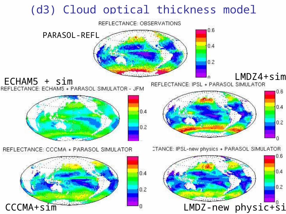
(d3) Cloud optical thickness model evaluation

PARASOL-REFL

ECHAM5 + sim

CCCMA+sim

LMDZ4+sim

LMDZ-new physic+sim

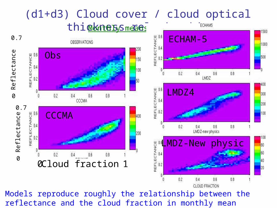
(d1+d3) Cloud cover / cloud optical thickness relationship

0.8

Ref

lect

ance

0.7

0 01 1

Monthly means

Observations LMDZ4 + Sim. LMDZ new physics+ Sim.

Obs

CCCMA

Cloud fraction

ECHAM-5

LMDZ4

LMDZ-New physicRef

lect

ance

0.7

00 1

Models reproduce roughly the relationship between the reflectance and the cloud fraction in monthly mean

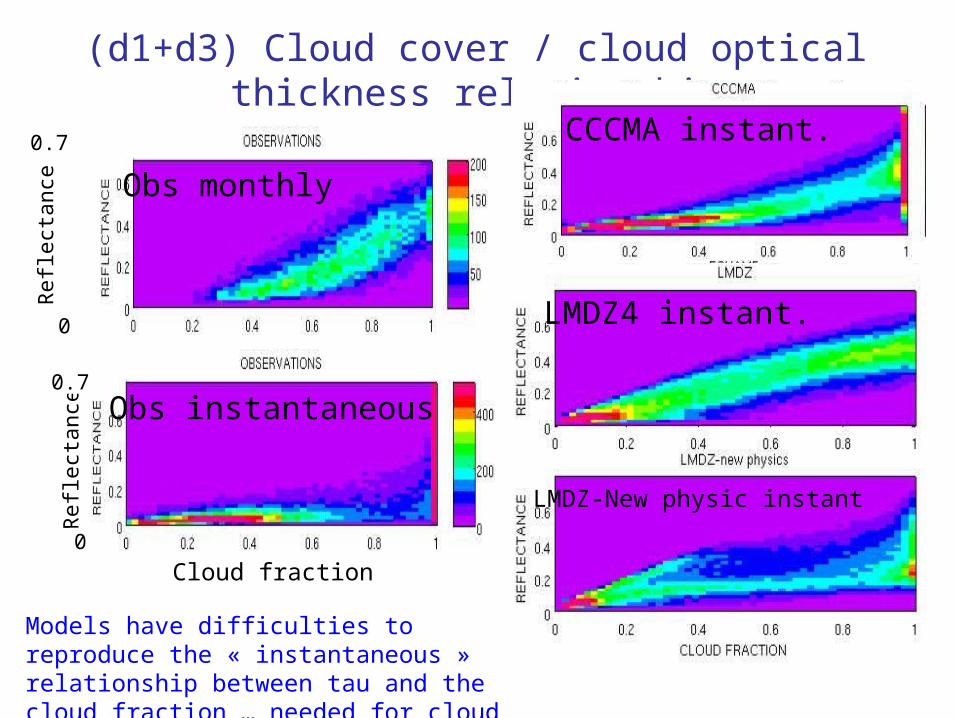
(d1+d3) Cloud cover / cloud optical thickness relationship

Ref

lect

ance

0.7

0

Observations LMDZ4 + Sim. LMDZ new physics+ Sim

Cloud fraction

Obs instantaneous

CCCMA instant.

LMDZ4 instant.

LMDZ-New physic instantRef

lect

ance

0.7

0

Obs monthly

Models have difficulties to reproduce the « instantaneous » relationship between tau and the cloud fraction … needed for cloud feedbacks

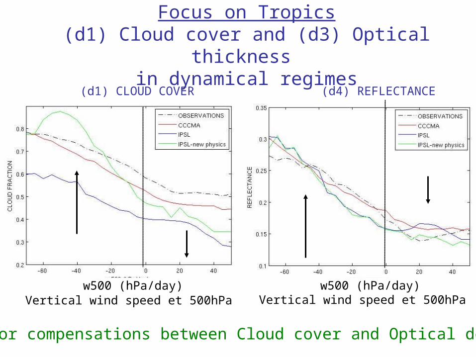
Focus on Tropics(d1) Cloud cover and (d3) Optical thickness

in dynamical regimes

(d4) REFLECTANCE

w500 (hPa/day)

(d1) CLOUD COVER

w500 (hPa/day)

Error compensations between Cloud cover and Optical depth

Vertical wind speed et 500hPa Vertical wind speed et 500hPa

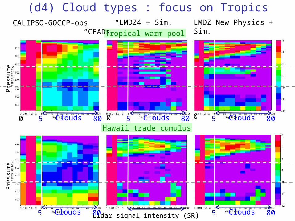
(d4) Cloud types : focus on Tropics

Tropical warm pool

Hawaii trade cumulus

LMDZ4 + Sim.CALIPSO-GOCCP-obs “CFADs”

LMDZ New Physics + Sim.

Pre

ssur

e

Lidar signal intensity (SR)

Clouds0 805 00

Pre

ssur

e

Clouds 805 Clouds 805

Clouds 805 Clouds 805

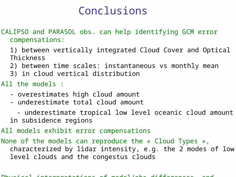
Conclusions

CALIPSO and PARASOL obs. can help identifying GCM error compensations:

1) between vertically integrated Cloud Cover and Optical Thickness2) between time scales: instantaneous vs monthly mean3) in cloud vertical distribution

All the models :

- overestimates high cloud amount- underestimate total cloud amount

- underestimate tropical low level oceanic cloud amount in subsidence regions

All models exhibit error compensations

None of the models can reproduce the « Cloud Types », characterized by lidar intensity, e.g. the 2 modes of low level clouds and the congestus clouds

Physical interpretations of model/obs differences and inter-model differences … just starts now

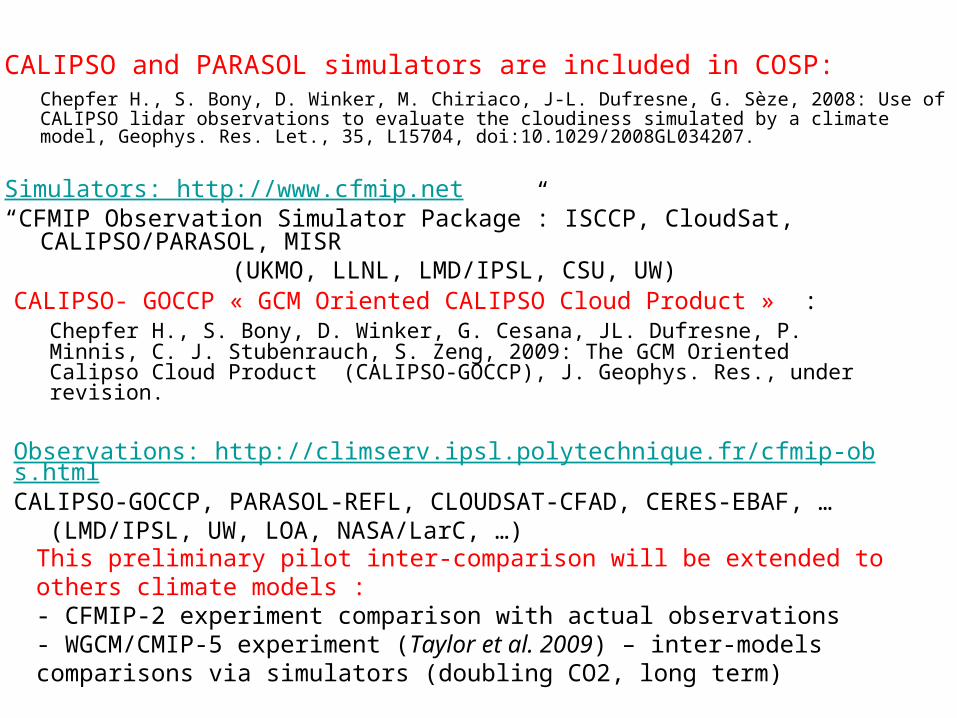
CALIPSO and PARASOL simulators are included in COSP:Chepfer H., S. Bony, D. Winker, M. Chiriaco, J-L. Dufresne, G. Sèze, 2008: Use of CALIPSO lidar observations to evaluate the cloudiness simulated by a climate model, Geophys. Res. Let., 35, L15704, doi:10.1029/2008GL034207.

Simulators: http://www.cfmip.net“CFMIP Observation Simulator Package”: ISCCP, CloudSat, CALIPSO/PARASOL, MISR

(UKMO, LLNL, LMD/IPSL, CSU, UW)

This preliminary pilot inter-comparison will be extended to others climate models : - CFMIP-2 experiment comparison with actual observations- WGCM/CMIP-5 experiment (Taylor et al. 2009) – inter-models comparisons via simulators (doubling CO2, long term)

Today, about 20 models use COSP (CFMIP Obs. Simulator Package)-

CALIPSO- GOCCP « GCM Oriented CALIPSO Cloud Product » :Chepfer H., S. Bony, D. Winker, G. Cesana, JL. Dufresne, P. Minnis, C. J. Stubenrauch, S. Zeng, 2009: The GCM Oriented Calipso Cloud Product (CALIPSO-GOCCP), J. Geophys. Res., under revision.

Observations: http://climserv.ipsl.polytechnique.fr/cfmip-obs.htmlCALIPSO-GOCCP, PARASOL-REFL, CLOUDSAT-CFAD, CERES-EBAF, …

(LMD/IPSL, UW, LOA, NASA/LarC, …)

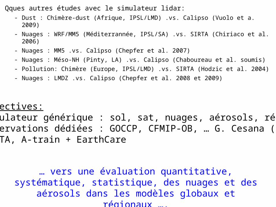
Qques autres études avec le simulateur lidar:- Dust : Chimère-dust (Afrique, IPSL/LMD) .vs. Calipso (Vuolo et a. 2009)

- Nuages : WRF/MM5 (Méditerrannée, IPSL/SA) .vs. SIRTA (Chiriaco et al. 2006)

- Nuages : MM5 .vs. Calipso (Chepfer et al. 2007)

- Nuages : Méso-NH (Pinty, LA) .vs. Calipso (Chaboureau et al. soumis)

- Pollution: Chimère (Europe, IPSL/LMD) .vs. SIRTA (Hodzic et al. 2004)

- Nuages : LMDZ .vs. Calipso (Chepfer et al. 2008 et 2009)

Perspectives:- Simulateur générique : sol, sat, nuages, aérosols, régional,- Observations dédiées : GOCCP, CFMIP-OB, … G. Cesana (Cdd)- SIRTA, A-train + EarthCare

… vers une évaluation quantitative, systématique, statistique, des nuages et des aérosols dans les modèles globaux et

régionaux ….

fin

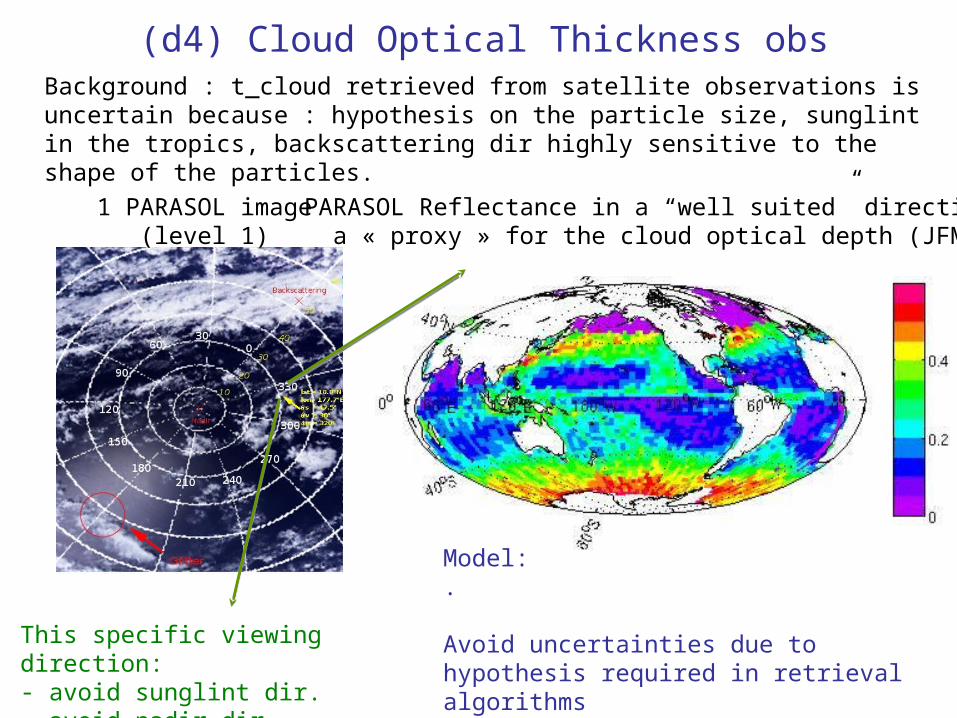
(d4) Cloud Optical Thickness obs

PARASOL Reflectance in a “well suited” direction :a « proxy » for the cloud optical depth (JFM)

1 PARASOL image(level 1)

This specific viewing direction:- avoid sunglint dir.- avoid nadir dir.- avoid backscattering dir.

Model:.

Avoid uncertainties due to hypothesis required in retrieval algorithms

Background : t_cloud retrieved from satellite observations is uncertain because : hypothesis on the particle size, sunglint in the tropics, backscattering dir highly sensitive to the shape of the particles.

23

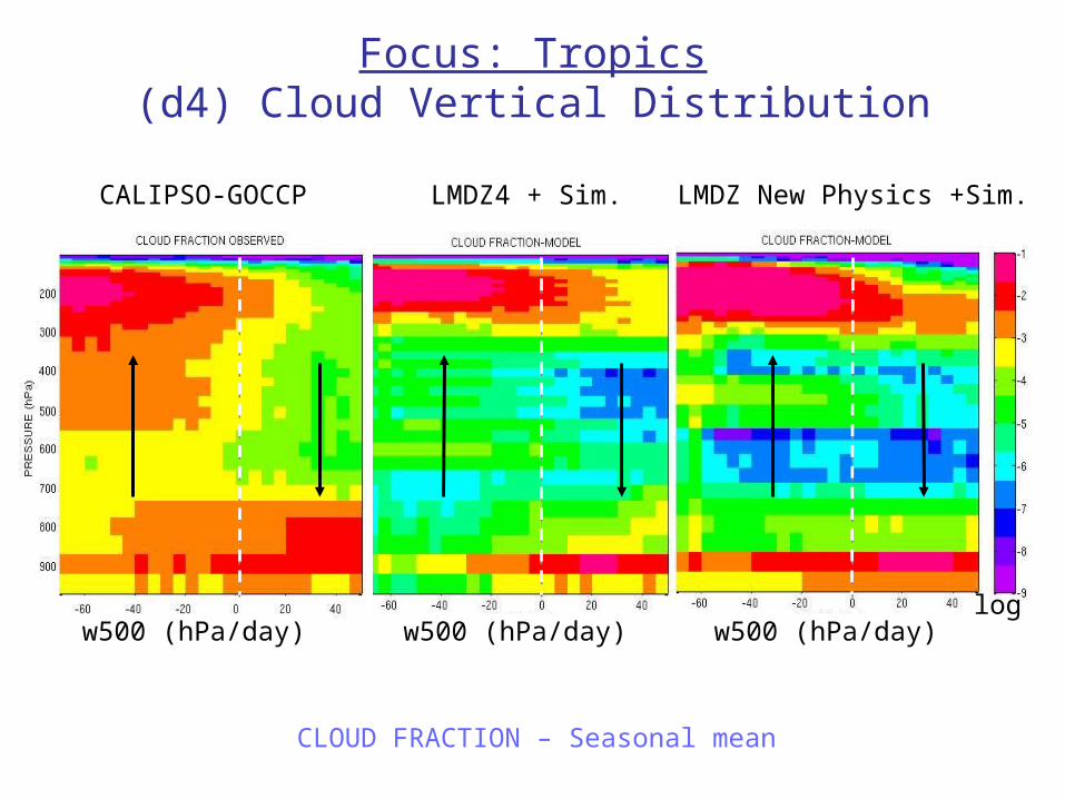
Focus: Tropics(d4) Cloud Vertical Distribution

CLOUD FRACTION – Seasonal mean

LMDZ4 + Sim.CALIPSO-GOCCP LMDZ New Physics +Sim.

logw500 (hPa/day) w500 (hPa/day)w500 (hPa/day)

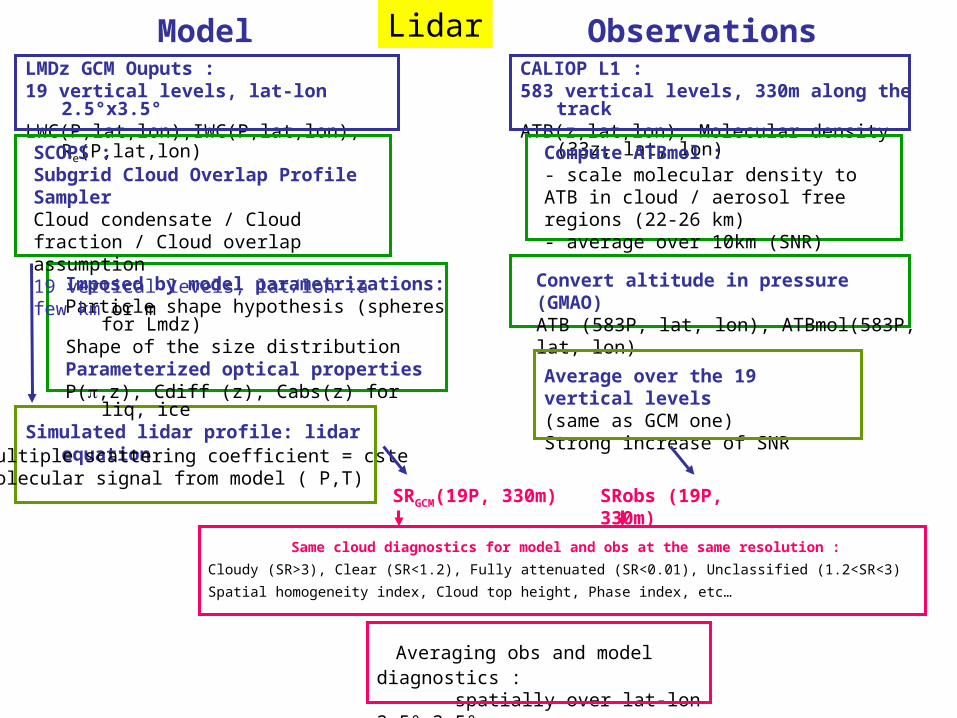
ModelLMDz GCM Ouputs : 19 vertical levels, lat-lon 2.5°x3.5°LWC(P,lat,lon),IWC(P,lat,lon), Re(P,lat,lon)

Simulated 1dir radiance

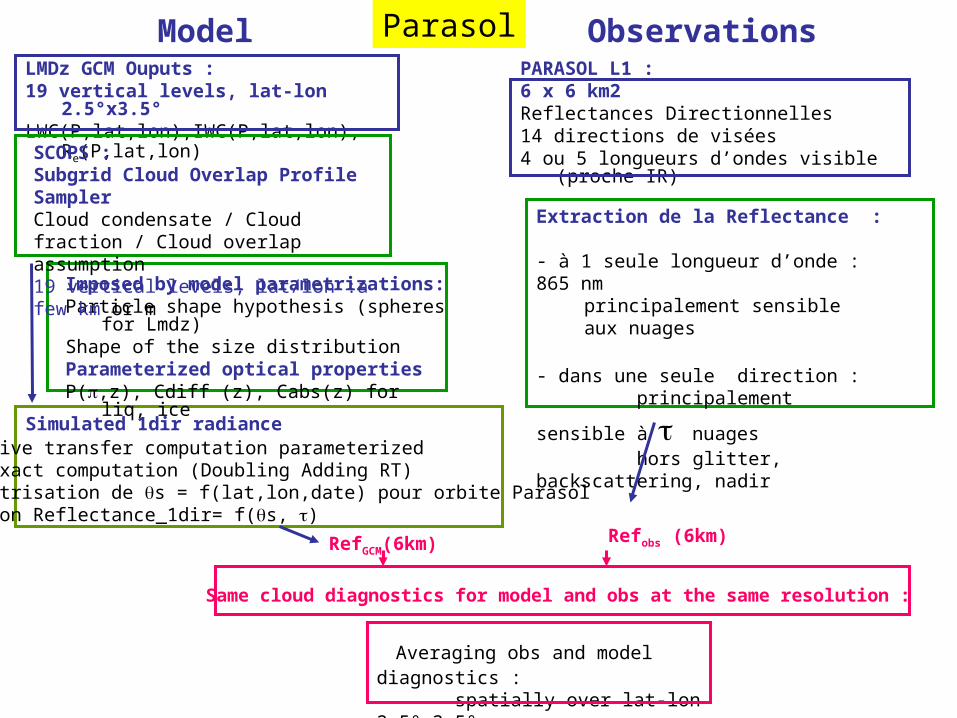
Imposed by model parametrizations:Particle shape hypothesis (spheres for Lmdz)Shape of the size distributionParameterized optical propertiesP(,z), Cdiff (z), Cabs(z) for liq, ice

SCOPS :Subgrid Cloud Overlap Profile SamplerCloud condensate / Cloud fraction / Cloud overlap assumption19 vertical levels, lat/lon :a few km or m

Radiative transfer computation parameterizedfrom exact computation (Doubling Adding RT)Parametrisation de s = f(lat,lon,date) pour orbite ParasolRelation Reflectance_1dir= f(s, )

PARASOL L1 : 6 x 6 km2Reflectances Directionnelles 14 directions de visées4 ou 5 longueurs d’ondes visible (proche IR)

Extraction de la Reflectance :

- à 1 seule longueur d’onde : 865 nm principalement sensible aux nuages

- dans une seule direction :

principalement sensible à nuages hors glitter, backscattering, nadir

Observations

RefGCM(6km) Refobs (6km)

Same cloud diagnostics for model and obs at the same resolution :

Averaging obs and model diagnostics : spatially over lat-lon 2.5°x3.5° temporally (month, season)

Parasol

ModelLMDz GCM Ouputs : 19 vertical levels, lat-lon 2.5°x3.5°LWC(P,lat,lon),IWC(P,lat,lon), Re(P,lat,lon)

Simulated lidar profile: lidar equation

Imposed by model parametrizations:Particle shape hypothesis (spheres for Lmdz)Shape of the size distributionParameterized optical propertiesP(,z), Cdiff (z), Cabs(z) for liq, ice

SCOPS :Subgrid Cloud Overlap Profile SamplerCloud condensate / Cloud fraction / Cloud overlap assumption19 vertical levels, lat/lon :a few km or m

Multiple scattering coefficient = csteMolecular signal from model ( P,T)

CALIOP L1 : 583 vertical levels, 330m along the trackATB(z,lat,lon), Molecular density (33z, lat, lon)

Compute ATBmol :- scale molecular density to ATB in cloud / aerosol free regions (22-26 km)- average over 10km (SNR)

Convert altitude in pressure (GMAO)ATB (583P, lat, lon), ATBmol(583P, lat, lon)

Observations

SRGCM(19P, 330m)

Average over the 19 vertical levels (same as GCM one)Strong increase of SNR

SRobs (19P, 330m)

Same cloud diagnostics for model and obs at the same resolution :

Cloudy (SR>3), Clear (SR<1.2), Fully attenuated (SR<0.01), Unclassified (1.2<SR<3)

Spatial homogeneity index, Cloud top height, Phase index, etc…

Averaging obs and model diagnostics : spatially over lat-lon 2.5°x3.5° temporally (month, season)

Lidar

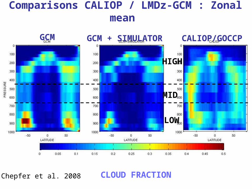
Comparisons CALIOP / LMDz-GCM : Zonal mean

GCM GCM + SIMULATOR CALIOP/GOCCP

CLOUD FRACTION

LOW

MID

HIGH

Chepfer et al. 2008

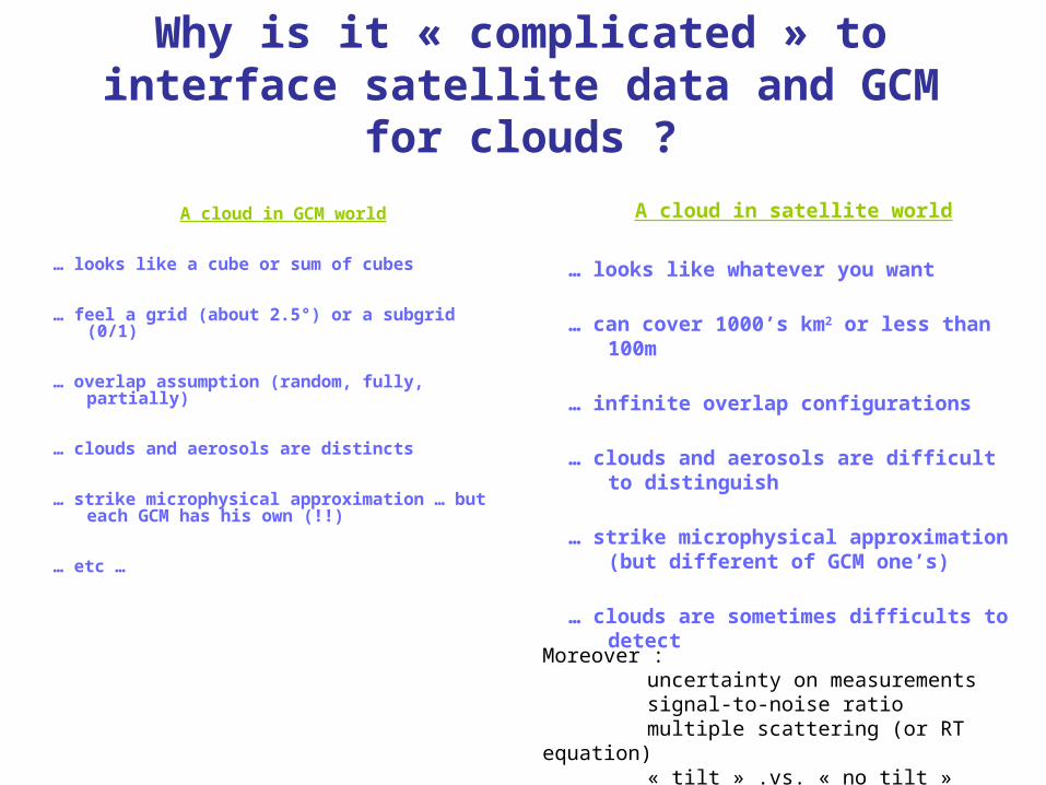
Why is it « complicated » to interface satellite data and GCM for clouds ?

A cloud in GCM world

… looks like a cube or sum of cubes

… feel a grid (about 2.5°) or a subgrid (0/1)

… overlap assumption (random, fully, partially)

… clouds and aerosols are distincts

… strike microphysical approximation … but each GCM has his own (!!)

… etc …

A cloud in satellite world

… looks like whatever you want

… can cover 1000’s km2 or less than 100m

… infinite overlap configurations

… clouds and aerosols are difficult to distinguish

… strike microphysical approximation (but different of GCM one’s)

… clouds are sometimes difficults to detect

Moreover :uncertainty on measurementssignal-to-noise ratiomultiple scattering (or RT equation)« tilt » .vs. « no tilt »

29

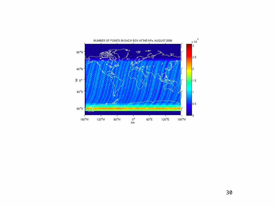
30

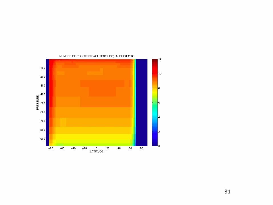
31

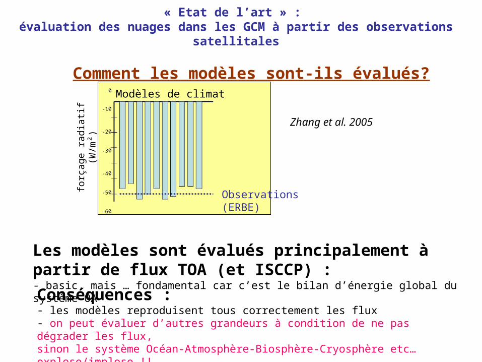
« Etat de l’art » : évaluation des nuages dans les GCM à partir des observations satellitales

Comment les modèles sont-ils évalués?

Observations (ERBE)

0

-10

-20

-30

-40

-50

-60

Modèles de climatfo

rçag

e ra

dia

tif (

W/m

²)

Zhang et al. 2005

Les modèles sont évalués principalement à partir de flux TOA (et ISCCP) :- basic, mais … fondamental car c’est le bilan d’énergie global du système OAConséquences :- les modèles reproduisent tous correctement les flux- on peut évaluer d’autres grandeurs à condition de ne pas dégrader les flux,sinon le système Océan-Atmosphère-Biosphère-Cryosphère etc… explose/implose !!

(dans le modèle)

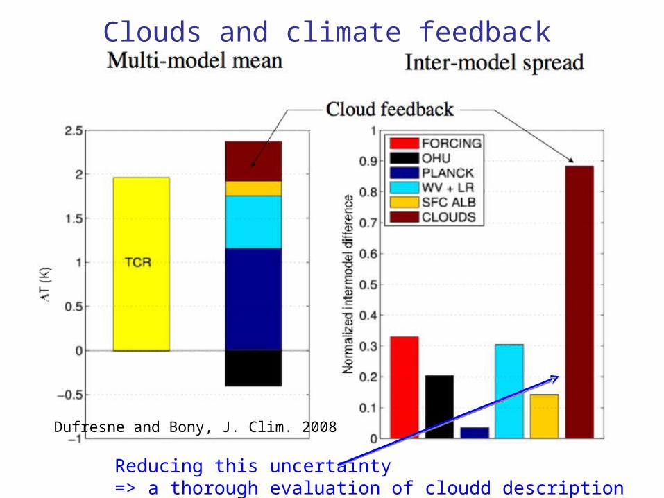
Clouds and climate feedback

Dufresne and Bony, J. Clim. 2008

Reducing this uncertainty => a thorough evaluation of cloudd description in climate models