Embed Size (px)
Citation preview

1
Evaluation of coefficient of friction in bulk metal forming*
Soheil Solhjoo†
Faculty of Mathematics and Natural Sciences, University of Groningen, Groningen, The Netherlands
Abstract
In this study an upper bound analysis for cylindrical "Barrel Compression Test" (BCT) is
developed. BCT method is a very simple method which can be utilized in order to
evaluate quantitatively the coefficient of friction by means of just one cylindrical
specimen in an upsetting test. The method is checked by a series of finite element
method (FEM) simulations and by means of the results of FEM simulations the method
is modified.
Keywords: Barrel Compression Test; bulk deformation; coefficient of friction; upper
bound method; finite element simulation.
1-Introduction:
The most accepted ways of characterizing friction quantitatively are to define a
coefficient of friction or a friction factor at the die/workpiece interface. There are
many researchers studied on the interface friction and readers may find some good
introductory in references [1-2].
* Written in summer of 2010, at Department of Materials Science and Engineering, Sharif University of
Technology, Tehran, Iran.

2
The upsetting at room temperature is one of the most widely used workability tests. As
the sample is compressed in the presence of friction, it tends to barrel. Variation of the
friction conditions and of the upset cylinder’s aspect ratio makes changes on the barrel
curvature. Avitzur [3] analyzed the barrel compression test (BCT) by means of upper
bound theorem and found a relationship between b (which was introduced as an
arbitrary coefficient) and the friction factor. Ebrahimi and Najafizadeh [1] proposed a
method in order to calculate the value of b and showed that there is a relationship
Nomenclature b the barrel parameter
H0 initial height of cylinder
H1 height of cylinder after deformation
ΔH reduction of height of cylinder after deformation
k, k current and mean shear yield stress of material, respectively
m constant friction factor
P average external pressure applied to cylinder in compression
R, θ, y general cylindrical coordinate
R0 initial radius of cylinder
RM, RT maximum and top radius of cylinder after deformation
R average radius of cylinder after deformation
ΔR difference between maximum and top radius
∑R summation of maximum and top radius
SD velocity discontinuity surface
SF friction surface
U die velocity
U , RU , yU velocity components in cylindrical coordinate
V volume of deformation zone
Sv magnitude of sliding velocity on SF
tv magnitude of velocity discontinuity tangent to SD
tW upper bound applied power
iW , fW , sW power dissipation due to internal deformation, friction, internal velocity
discontinuity and external traction force, respectively
Y flow stress of material
ij components of strain rate tensor
equivalent strain rate
µ Coulomb coefficient of friction
µc calculated coefficient of friction from the simulations
τ shear stress

3
between b and barrel curvature. Very recently, Solhjoo [4] utilized their method and
showed that the results of this method need some modifications.
Usually the calculations of metal forming analyses facilitate using the friction factor but
most of the computer simulation programs use the coefficient of friction. Therefore, it
is important to determine the coefficient of friction of interfaces precisely in order to
have a reliable simulation. In this study using the upper bound theorem, the BCT
method is analyzed and a relationship is derived which can be used to determine the
coefficient of friction. Afterwards, a series of finite element method (FEM) simulations
are done in order to check the derived formula. Using the results, the model is
modified. The major advantage of the BCT method is that it involves only the physical
measurement of the changes in shape.
2-Coulomb coefficient of friction
A relative motion between two bodies in contact provides a resistance to this motion
which is called friction. The surface area of contact is a boundary of the deformed
metal. Thus, the friction resistance is also the shear stress in the material at its
boundary. If the friction is assumed to obey coulomb’s law, then:
1P
The shear stress at any point on that surface is proportional to the pressure (P)
between the two bodies and is directed opposite to relative motion between those
bodies. Since the value of P is different at any point, the value of coefficient of friction
would be different for each point. As a result, any calculations will be far too complex.
In order to solve this problem an average value for the pressure can be defined which
leads to a single mean value for coefficient of friction and also taken as a constant for a
given die and material (under constant surface and temperature conditions). This value
is also considered independent of velocity [3].

4
3-Evaluation of coefficient of friction
The value of coefficient of friction could be obtained by two different procedures. First
one is to calculate the value of coefficient of friction from the constant friction factor.
This method starts from two different formulae for shear stress ( mkP ). In BCT
the value of P evaluates as follows:
233
21
1
H
RmYP
where 1
0
0H
HRR [1] determined from volume constancy. Using von Mises’ yield
criterion one can find kY 3 which leads to:
33
23
1H
Rmm
k
P
By means of this equation the value of coefficient of friction can be easily found from
constant friction factor.
4
233
3
1
H
Rm
m
Additionally, it is possible to analyze BCT by means of the upper bound theorem in
order to determine the value of the coefficient of friction directly from the test results
without undue calculations of constant friction factor.
5
4-Upper bound method
The upper bound method (UBM) is based on the energy principle known as the upper
bound theorem [5]. The upper bound theorem states that the rate of total energy
associated with any kinematically admissible velocity field defines an upper bound to
the actual rate of total energy required for the deformation. Hence, for a given class of
kinematically admissible velocity fields the velocity field that minimizes the rate of
total energy is the lowest upper bound and therefore is nearest to the actual solution.
The upper bound theorem was formulated by Prager and Hodge [6] and later modified
by Drucker et al. [7-9] by including the velocity discontinuities. Kudo [10] introduced
the concept of dividing the workpiece into several rigid blocks, obtaining lower upper
bounds by changing the shape and number of these blocks. Kobayashi and Thomsen
[11] suggested curved discontinuity surfaces for the deformation blocks which gave
better upper bounds for some axisymmetric problems. The upper bound theorem
states that the actual energy rate is less than or equal to:
aWWWW sfit 5
bdVkWV
i 52
cdSvW
FS
Sf 5
ddSvkW
DS
ts 5
where can be determined by Eq.6:
621
ijij
6
The third term of Eq.5a (SW ), also known as the jump condition, can be omitted when
a class of continuous velocity fields is considered [5].
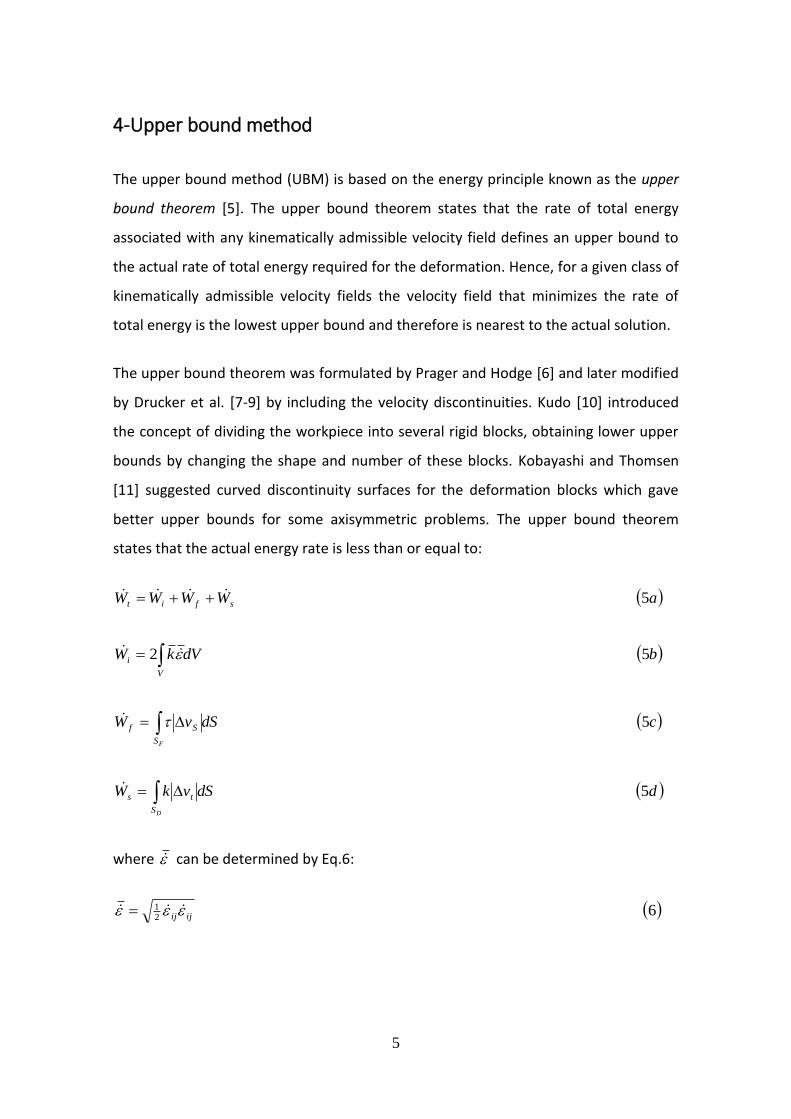
5-Analysis of BCT
The coordinates system applied to a solid disk is plainly illustrated in Fig.1. Two anvils
move toward each other at the same absolute velocity. Since the radial component of
velocity (RU ) in the center of the disk (y=0) is larger than
RU at the friction surfaces
(surfaces in contact with anvils i.e. y=±H1/2), the cylinder barrels out during the
compression.
Fig.1. A simple representation of barrel compression test. (upper) coordinates system,
(lower) the disk after upsetting.

7
As Avitzur clarified [3] friction reduces velocity components on the platen surfaces
which lead to reduced friction loss. But since RU changes over the thickness of the
billet, a shear component introduces which increases the internal power of
deformation. Because of this, the velocity at the die surface may decreases but does
not drop to zero. To sum up, bulging produces a slightly lower total energy.
In order to make the paper easier to read, the whole mathematical steps taken for the
analysis of BCT by means of UBM is written in appendix A. The analysis results in the
following equation which can be used in order to evaluate the value of coefficient of
friction.
7
1212
3
2
1
1
H
Rb
H
Rb
where the value of b defines as [4]:
8124 1
H
H
R
Rb
6-Examination of BCT method
Finite element method (FEM) is employed to check the correctness of BCT method.
6.1-Finite element method
The FEM was conducted using DEFORM-2D V9.0 software (Scientific Forming
Technologies Corp.) and a series of simulations of upsetting tests were performed. Due

8
to the axisymmetric profile of the simulation, only one half of each cylindrical billet and
die was modeled. The value of H0 and R0 were selected as 16 and 5mm, respectively. -
Using the materials library of the software, aluminum (Al-6063) was selected as the
material of the billet. Rigid bodies were suggested for the upper and lower platens to
reduce the running time during the simulations.
6.2-Simulation control of upsetting process
In these simulations, the coordinates system’s perpendicular direction was set as y-
axis. During the upsetting process, the upper die, which was primary die, with a given
speed moved along the negative y-axis and the billet was placed between the moving
upper and the still lower platens.
6.3-Simulation procedures
Different final heights (between 15 and 12mm with 1mm steps) and different
coefficients of friction (0.01, 0.03, 0.05, 0.07, 0.1, 0.2, 0.3, 0.4, 0.5 and 0.577) were
selected for simulations.
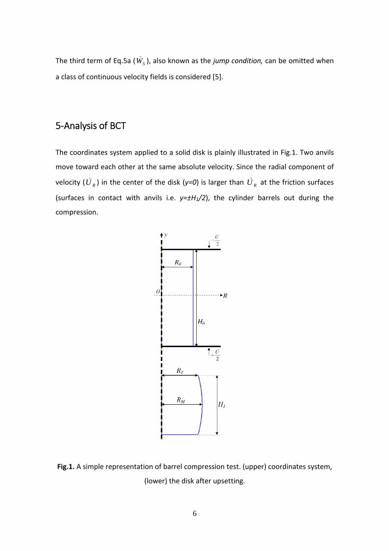
7-Results and discussion
After each simulation the values of RM and RT were measured and consequently the
values of parameter b and coefficient of friction were calculated. The values of RM, RT,
parameter b and µ are listed in table 1.
9
Table 1. The measured and calculated values of RM, RT, b and µc from the simulations
performed under different constant friction factors with different final heights.
µ 0.01 0.03 0.05 0.07 0.1 0.2 0.3 0.4 0.5 0.577
H1 15
RM 5.166 5.173 5.180 5.186 5.195 5.220 5.229 5.230 5.230 5.230
RT 5.156 5.143 5.129 5.117 5.100 5.052 5.027 5.021 5.020 5.020
B 0.112 0.337 0.574 0.777 1.070 1.897 2.285 2.365 2.377 2.377
µc 0.010 0.031 0.054 0.075 0.109 0.226 0.296 0.312 0.314 0.314
H1 14
RM 5.347 5.355 5.363 5.37 5.382 5.418 5.437 5.44 5.44 5.441
RT 5.333 5.312 5.292 5.271 5.241 5.144 5.082 5.073 5.069 5.066
B 0.068 0.210 0.347 0.484 0.690 1.349 1.755 1.815 1.836 1.856
µc 0.007 0.021 0.035 0.050 0.073 0.159 0.223 0.234 0.237 0.241
H1 13
RM 5.550 5.562 5.574 5.586 5.602 5.651 5.671 5.674 5.675 5.675
RT 5.528 5.497 5.465 5.434 5.388 5.235 5.190 5.179 5.173 5.170
B 0.061 0.180 0.303 0.423 0.597 1.172 1.358 1.399 1.419 1.428
µc 0.007 0.020 0.034 0.048 0.069 0.149 0.178 0.184 0.188 0.189
H1 12
RM 5.777 5.795 5.813 5.829 5.853 5.918 5.938 5.941 5.943 5.943
RT 5.747 5.703 5.659 5.615 5.548 5.345 5.300 5.289 5.276 5.271
B 0.052 0.160 0.268 0.374 0.535 1.017 1.135 1.161 1.189 1.199
µc 0.006 0.020 0.033 0.047 0.069 0.141 0.160 0.164 0.169 0.170
10
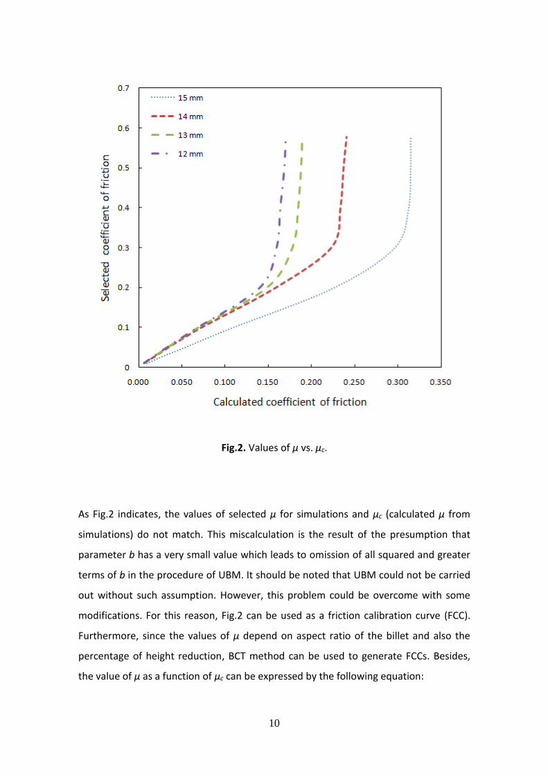
Fig.2. Values of µ vs. µc.
As Fig.2 indicates, the values of selected µ for simulations and µc (calculated µ from
simulations) do not match. This miscalculation is the result of the presumption that
parameter b has a very small value which leads to omission of all squared and greater
terms of b in the procedure of UBM. It should be noted that UBM could not be carried
out without such assumption. However, this problem could be overcome with some
modifications. For this reason, Fig.2 can be used as a friction calibration curve (FCC).
Furthermore, since the values of µ depend on aspect ratio of the billet and also the
percentage of height reduction, BCT method can be used to generate FCCs. Besides,
the value of µ as a function of µc can be expressed by the following equation:

11
9exp 321 cc uuu
where u1, u2 and u3 are constants which have different values for different reduction in
heights. The calculated values for these three constants based on the applied
simulations are listed in table 2. It is considerable in Fig.2, lower reduction in height
results in higher accuracy of calculations and also acquires a wider range for µc that
make it easier to use the FCCs.
Table 2. The values of u1, u2 and u3 at different final heights
H1 (mm) %Reduction
in height u1(×10-8) u2 u3
15 6.25 5.917 48.28 0.8536
14 12.5 6.811×10⁻² 81.95 1.235
13 18.75 6.548 80.88 1.282
12 25 7.704×10⁻¹ 103.2 1.351
8-Conclusion
In this paper the barrel compression test is analyzed by means of UBM and a formula is
derived for evaluation of coefficient of friction quantitatively from BCT method. The
method was tested by a series of FEM simulations (for Al-6063) which showed that this
method needs to be modified. This modification can be done using FCCs or Eq.9. Also,
it showed that this method can be used to generate FCCs in order to determine the
coefficient of friction at the die/workpiece interface in large deformation processes. In
addition, it is noted that upsetting under low percentage of reduction in height yields
more reliable and accurate results.

12
9-Appendix A
The axes of a cylindrical coordination system are the radial direction R, the
circumferential direction θ and the direction of the axis of symmetry y. The velocity is
yR UUUU ,, while the strain rate components ij acquire the subscripts R, θ and y.
The strain rates as functions of the velocity components are:
aAR
URRR 1
bAU
RR
UR 11
cAy
U y
yy 1
dAR
U
R
UU
R
RR 1
1
2
1
eAU
Ry
U y
y 11
2
1
fAR
U
y
U yRyR 1
2
1
The axes were chosen as shown in Fig.1. The origin of the cylindrical coordinate system
is at the center of the disk. The two platens are considered rigid bodies and move
toward each other at the same absolute velocity (2
U). Because of symmetry and to
ease computation, the upper half of the disk is considered. Assume a velocity field [3]
for 2
0 1Hy only
aAU 20
bAH
by
H
RUAUR 2exp
11
cAyRUU yy 2,
13
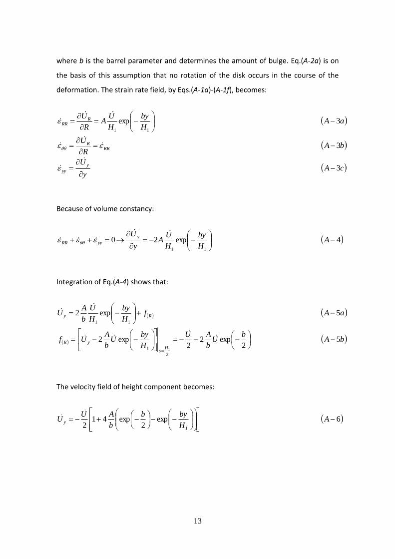
where b is the barrel parameter and determines the amount of bulge. Eq.(A-2a) is on
the basis of this assumption that no rotation of the disk occurs in the course of the
deformation. The strain rate field, by Eqs.(A-1a)-(A-1f), becomes:
aAH
by
H
UA
R
URRR 3exp
11
bAR
URR
R 3
cAy
U y
yy 3
Because of volume constancy:
4exp2011
A
H
by
H
UA
y
U y
yyRR
Integration of Eq.(A-4) shows that:
aAfH
by
H
U
b
AU Ry 5exp2
11
bAb
Ub
AU
H
byU
b
AUf
Hy
yR 52
exp22
exp2
2
1 1
The velocity field of height component becomes:
6exp2
exp412 1
A
H
byb
b
AUU y
14
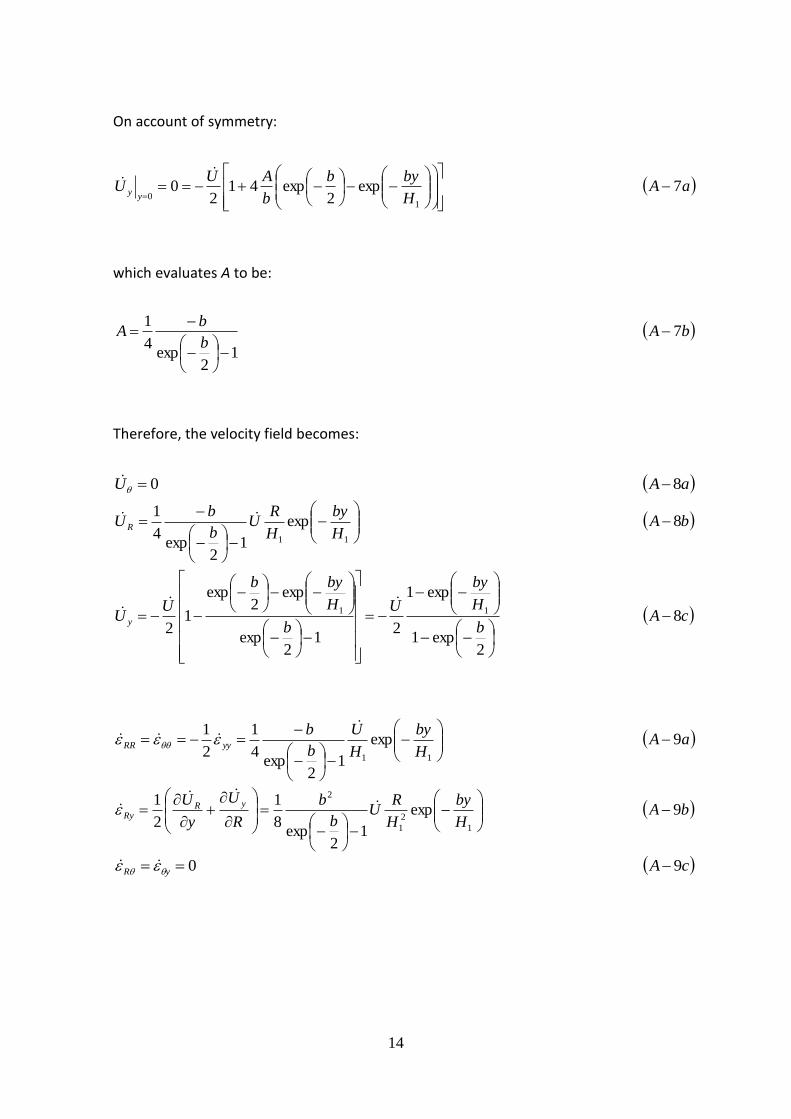
On account of symmetry:
aAH
byb
b
AUU
yy 7exp
2exp41
20
10
which evaluates A to be:
bAb
bA 7
12
exp4
1
Therefore, the velocity field becomes:
aAU 80
bAH
by
H
RU
b
bU R 8exp
12
exp4
1
11
cAb
H
by
U
b
H
byb
UU y 8
2exp1
exp1
21
2exp
exp2
exp
12
11
aAH
by
H
U
b
byyRR 9exp
12
exp4
1
2
1
11
bAH
by
H
RU
b
b
R
U
y
U yRRy 9exp
12
exp8
1
2
1
1
2
1
2
cAyR 90

15
By using Eqs.(A-9a)-(A-9c) the internal power of deformation becomes:
aAdVYdVYWV
RyRRV
ijiji 1033
2
2
1
3
2 22
where dydRRdV 2 . Therefore:
bAdydRH
RbR
H
by
b
b
T
UYW
Hy
oy
R
Ri 10
4
13exp
12
exp4
22
3
22
0 2
1
22
1
1
cAb
H
Rb
H
RRb
T
UYWi 10
12121
33
2
3
2
2
1
2
2
3
2
2
1
2
3
Minimum iW is obtained for b=0 and it represents the ideal power of deformation
where there is no bulging in the specimen. But in actual solution 0b and the internal
power of deformation as computed by Eq.(A-10c) is higher than the ideal value.
The friction loss is:
aAdRRH
U
b
b
bPRdRUPWR
R
R
RH
yRf 11
12
exp
2exp
40
2
10
2
1
Multiplying the numerator and denominator of Eq.(A-11a) by
2exp
b results in:
bAb
RbT
UPW f 11
2exp1
1
3
3

16
The external power is supplied by two platens and equals:
122
2. 22 APURU
PRWt
Equating the external power with the internal power of deformation plus friction loss,
one obtains:
aAbH
Rb
Y
P
b
H
Rb
H
RH
Rb
YUR
W
Y
P t
13
2exp1
1
3
112121
33
1
1
2
3
2
2
1
2
2
3
2
2
1
2
1
2
This can be simplified to:
bAM
S
bH
Rb
b
H
Rb
H
RH
Rb
Y
P13
12
exp
1
3
11
12121
33
1
1
2
3
2
2
1
2
2
3
2
2
1
2
1
where S and M stand as numerator and denominator of Eq.(A-13b). S can be rearrange
as follows:
14112
11
18
11
12
18
2
3
2
2
1
2
2
1
3
3
1
2
3
2
2
1
1
Ab
H
R
bR
H
bR
H
bR
Hb
H
RS
Since the actual shape of disk is such that the required power is minimized, to have
minimum value of P the optimum b must be chosen. The value minimizing the
17
pressure can be determined by successive approximations directly from the above
equation. Differentiating the above equation with respect to b and equating the
derivative to zero results in an implicit equation which offers no advantage over Eq.(A-
14). But some advantage can be gained by substituting the proper series expansions as
follows. First let’s define two variables as follows:
aAbH
R
b
Cb
H
RC 15
6
1
12
12
1
2
2
1
bAb
b15
2
1
2
Therefore, S and M become:
aACC
S 16111
3
22
3
bA
H
R
b
b
H
RM 16
1exp3
21
12
exp
2
3
21
11
In order to solve Eqs.(A-16a) and (A-16b) two following series expansions are needed:
aACCCCCC 17...10
5
8
3
6
1
4
1
2
3
8
3
6
1
4
1
2
3
6
1
4
1
2
3
4
1
2
3
2
311 5432
2
3
bA
n
B
n
n
n 17!1exp 0
where Bn’s are called Bernoulli’s numbers and sometimes called even-index Bernoulli
numbers. The first few Bernoulli numbers (Bn) are 10 B , 2
11 B ,
6
12 B ,
30
14 B ,
42
16 B and
30
18 B . Expanding the series, S and M become:

18
aACCCCS 18...10
5
8
3
6
1
4
1
8
3
6
1
4
1
6
1
4
1
4
11 432
bAH
RM 18...
!830
1
!642
1
!430
1
!26
1
21
3
21
8642
1
The expression M
S
Y
P can be differentiated with respect to b and the derivative can
be equated to zero for the optimum value of b.
1902
A
b
MS
b
SM
M
b
MS
b
SM
Y
P
b
aAbH
Rb
H
Rb
H
R
b
CCC
b
S
206
1...
144
1
64
3
144
1
4
1
...38
3
6
1
4
12
6
1
4
1
4
1
2
1
4
4
1
2
2
1
2
bAbb
H
R
bH
R
b
M20...
1440122
1
3
1...
!4
4
30
1
!2
2
6
1
2
1
3
2 3
1
3
1
Substituting the expansions in b
MS
b
SM
and omitting all squared and greater
terms of b:
2106
1
36
1
24
1
36
1
11
2
1
3
1
A
H
Rb
H
R
H
R
H
R
This equation can be solved explicitly for the optimum b:
22
23
12
1
1
1
A
H
R
R
H
R
H
b

19
which with a rearrangement can be rewritten as follows:
23
1212
3
212
32
1
1
1
11
A
H
Rb
H
Rb
H
R
R
Hb
R
H
b
References
[1] R. Ebrahimi, A. Najafizadeh, A new method for evaluation of friction in bulk metal
forming, J. Mater. Process. Technol., 152 (2004) 136-143.
[2] H. Sofuoglu, H. Gedikli, Determination of friction coefficient encountered in large
deformation processes, Trib. Int., 35 (2002) 27-34.
[3] B. Avitzur, Metal Forming Processes and Analysis. 1968: McGraw-Hill.
[4] S. Solhjoo, A note on "Barrel Compression Test", Comput. Mater. Sci., 49 (2010)
435–438.
[5] W.T. Wu, J.T. Jinn, C.E. Fischer, Modeling Techniques in Forming Processes, in
Handbook of Workability and Process Design, G.E. Dieter, H.A. KuhnS.L.
Semiatin, Editors. 2003, ASM International: Material Parks, Ohio. p. 220-231.
[6] W. Prager, P.G. Hodge, Theory of Perfectly Plastic Solids. 1951, New York: Wiley.
[7] D.C. Drucker, H.J. Greenberge, W. Prager, The safety factor of an elastic-plastic
body in plane strain, J. Appl. Mech. Trans. ASME, 73 (1951) 371-378.
[8] D.C. Drucker, W. Prager, H.J. Greenberge, Extended limit design theorems for
continuous media, Quart. Appl. Math, 9 (1952) 381-389.
[9] D.C. Drucker, R.I. Providence, Coulomb friction, plasticity, and limit loads, J. Appl.
Mech, 21 (1954) 71-74.

20
[10] H. Kudo, An upper bound approch to plane-strain forging and extrusion- II, Int. J.
Mech. Sci., 1 (1960) 229-252.
[11] S. Kobayashi, E.G. Thomsen, Upper- and lower bound solutions to axisymmetric
compression and extrusion problems, Int. J. Mech. Sci., 7 (1965) 127-143.