Evaluation of Gas Insulated Lines (GIL) for Long Distance ...orca.cf.ac.uk/73315/1/2015ElnaddabKPhD.pdf · Evaluation of Gas Insulated Lines ... using an HVAC gas-insulated transmission

Evaluation of Gas Insulated Lines

(GIL) for Long Distance HVAC

Power Transfer

A thesis submitted to Cardiff University

in candidature for the degree of

Doctor of Philosophy

By

Khalifa Elnaddab

School of Engineering

Cardiff University

December 2014

DECLARATION

This work has not previously been accepted in substance for any degree and is not

concurrently submitted in candidature for any degree.

Signed……………..………… (Candidate) Date……………….

STATEMENT 1

This thesis is being submitted in partial fulfilment of the requirements for the

degree of PhD.


STATEMENT 2

This thesis is the result of my own independent work/investigation, except where

otherwise stated. Other sources are acknowledged by explicit references.


STATEMENT 3

I hereby give consent for my thesis, if accepted, to be available for photocopying

and for inter-library loan, and for the title and summary to be made available to

outside organisations.


STATEMENT 4

I hereby give consent for my thesis, if accepted, to be available for photocopying

and for inter-library loans after expiry of a bar on access previously approved by

the Graduate Development Committee.


In the name of Allah, the Most Gracious, the Most Merciful

Peace and blessings be upon our Prophet Muhammad

and upon his family and companions

ACKNOWLEDGEMENTS

First and foremost, I would like to thank the Almighty Allah for enabling me to

complete this work; peace and blessings be upon our Prophet Muhammad and

upon his family and companions.

I would like to express my extreme appreciation and sincere gratitude to my

supervisor, Professor Manu Haddad. His guidance, encouragement and advice

were essential in helping me to finish this work.

My sincere appreciation also goes to my second supervisor, Dr Huw Griffiths, for

his valuable advice and constructive criticism during our weekly meetings and

annual progress assessment.

I would also like to thank the following for their contributions:

Professor Abdelhafid BAYADI from Ferhat ABBAS University of Setif, Algeria

for his extensive knowledge and help in the EMTP simulation program

All the members of the academic and administrative staff of School of

Engineering, Cardiff University

Dr Alex Bogias, Dr Maurizio Albano, Dr David Clark, Fabian Moore, Dr

Muhammad Saufi Kamarudin, Philip Widger, Tony Chen, for valuable

discussions and for their friendship

And my special thanks to my wife, my daughter, and my parents for the selfless

patience and endless support which they have shown throughout the period of my

studies.

Lastly, I would like to thank my older brother Abu Baker for his financial support

during my PhD studies.

PUBLICATIONS

i. K. H. Elnaddab, A. Haddad, H. Griffiths, "The transmission

characteristics of gas insulated lines (GIL) over long distance,"

Universities Power Engineering Conference (UPEC), 2012 47th

International, vol., no., p.1,5, 4-7 Sept. 2012 doi:

10.1109/UPEC.2012.6398633

ii. K. H. Elnaddab, A. Haddad, H. Griffiths, ‘Future Gas Insulation Lines

for Transmission Networks’, Fifth Universities High Voltage Network

(UHVNet), 18-19 January 2012, Leicester, UK

iii. K. H. Elnaddab, L. Chen, M.S. Kamarudin, A. Haddad, and H.

Griffiths, ‘Gas Insulated Transmission Lines Using CF3I’, Sixth

Universities High Voltage Network (UHVNet), 16-17 January 2013,

Glasgow, UK

iv. M. S. Kamarudin, P. Widger, L. Chen, K. H. Elnaddab, A. Haddad, H.

Griffiths, ‘CF3I and Its Mixtures: Potential for Electrical Insulation’,

International Council on Large Electric Systems (CIGRE) Session 45,

D1-309_2014, Paris, France

SUMMARY

Offshore wind power is a key element in EU policies to reduce the greenhouse

effect and secure energy sources. In order to accomplish the EU’s target of a 20%

share of energy from renewable sources by 2020, some of the planned projects

have to be placed far away from the shoreline to benefit from the high wind

speeds in the open sea area.

However, a traditional transmission system for offshore wind farms based on a

High Voltage Alternating Current (HVAC) utilizing conventional cables is not

appropriate for long distances. In contrast, a High Voltage Direct Current

(HVDC) can transmit electrical power over such distances, but the complicated

concept of converting the HVAC offshore generated power into DC and then

converting the DC power at the onshore grid back to AC requires sophisticated

and expensive converter stations at both ends.

Therefore, developing a new infrastructure solution based on HVAC transmission

technology, which has been in operation for more than a century and which runs

almost entire electrical systems, to support and advance the development of

offshore wind energy is a highly desirable outcome.

This research work was conducted to examine and determine the suitability of

using an HVAC gas-insulated transmission line (GIL) as a long-distance

transmission system for offshore wind farms in terms of technical and economic

costs.

A computer model of GIL has been built using the Electromagnetic Transient

Program (EMTP) to assess the suitability of GIL and quantify the voltage, current

and power transfer characteristics of the GIL under different steady state

conditions. Furthermore, a suitable model has been developed for the simulation

of the switching transient during energisation of the GIL transmission system and

various wind farm components.

The development concept of GIL as a submarine Power Transmission Pipeline

(PTP) is described, and the practical side of installing the PTP technology and the

special design requirements of the offshore wind farms were illustrated. The PTP

components, the maximum transmission capacity of the PTP system and the

layout options were addressed. In addition, the challenges facing this technology

were discussed.

An economic comparison of the total cost for both HVAC-GIL and HVDC-VSC

transmission systems is made, including annual costs (operation, maintenance,

and losses) during the lifetime of the projects. The initial investment costs are

added to the annual costs in order to obtain the total cost for the assumed project.

Furthermore, the Power Transmission Cost (PTC) is calculated for each MVA-km

being delivered to the receiving end of the GIL transmission line.

Table of Contents

DECLARATION ........................................................................................................ ii

ACKNOWLEDGEMENTS ....................................................................................... ii

PUBLICATIONS ....................................................................................................... iii

SUMMARY ................................................................................................................ iv

CHAPTER 1: INTRODUCTION .......................................................................... 1-1

1.1 Introduction ........................................................................................... 1-1

1.2 Transmission System for Offshore Wind Frames ................................ 1-3

1.3 Research Objectives .............................................................................. 1-7

1.4 Contribution of Thesis .......................................................................... 1-8

1.5 The Structure of the Thesis ................................................................... 1-9

CHAPTER 2: OVERVIEW OF GAS-INSULATED TRANSMISSION LINE

(GIL) ......................................................................................................................... 2-1

2.1. Introduction ........................................................................................... 2-1

2.2. Definition and Description of GIL ....................................................... 2-2

2.3. History of Development ....................................................................... 2-3

2.3.1. First Generation of GIL ................................................................. 2-3

2.3.2. Second Generation of GIL ............................................................ 2-6

2.3.3. Alternative Gas to SF6 ................................................................... 2-9

2.4. GIL Design Criteria ............................................................................ 2-12

2.4.1. Dielectric Dimensioning .............................................................. 2-13

2.4.2. Thermal Dimensioning ................................................................ 2-14

2.4.3. Gas Pressure Dimensioning ......................................................... 2-14

2.4.4. High Voltage Tests Design .......................................................... 2-15

2.4.5. Short Circuit Rating Design ........................................................ 2-16

2.4.6. Internal Arc Design ..................................................................... 2-17

2.4.7. Mechanical Design ...................................................................... 2-18

2.4.8. Thermal Design ........................................................................... 2-19

2.5. GIL Component Design ...................................................................... 2-20

2.5.1. Technical Data ............................................................................. 2-20

2.5.2. Standard Units ............................................................................. 2-21

2.5.3. Electrical Parameters of GIL ....................................................... 2-23

2.5.4. Joint Technology ......................................................................... 2-24

2.6. Layout Methods .................................................................................. 2-24

2.6.1. Above Ground Installation .......................................................... 2-25

2.6.2. Directly Buried ............................................................................ 2-25

2.6.3. Tunnel Installation ....................................................................... 2-26

2.6.4. Vertical Installation ..................................................................... 2-26

2.7. Advantages of GIL ............................................................................. 2-26

2.7.1. High Transmission Capacity ....................................................... 2-26

2.7.2. Low Electrical Power Losses ...................................................... 2-27

2.7.3. High Level of Personnel Safety ................................................... 2-27

2.7.4. Natural Cooling Still Adequate at Over 3000 A ......................... 2-28

2.7.5. Low Magnetic Fields ................................................................... 2-28

2.8. Corrosion Protection ........................................................................... 2-29

2.9. System Control and Diagnostic Tools ................................................ 2-32

2.9.1. Gas Density Monitoring .............................................................. 2-32

2.9.2. Partial Discharge Measurement ................................................... 2-33

2.9.3. Temperature Measurement .......................................................... 2-34

2.10. Summary ......................................................................................... 2-34

CHAPTER 3: MODELLING OF GIL AND ASSOCIATED EQUIPMENT

IN THE ELECTRICAL NETWORK ................................................................... 3-1

3.1. Introduction ........................................................................................... 3-1

3.2. Line Models in EMTP .......................................................................... 3-1

3.3. Transmission Line Modelling ............................................................... 3-3

3.3.1. GIL Modelling ............................................................................... 3-3

3.3.2. XLPE Cable Modelling ................................................................. 3-5

3.3.3. Overhead Line Modelling ............................................................. 3-9

3.4. Transformer Modelling ....................................................................... 3-11

3.4.1. BCTRAN Model ......................................................................... 3-12

3.4.2. Linear BCTRAN Part Modelling ................................................ 3-12

3.4.3. Nonlinear BCTRAN Part ............................................................ 3-15

3.4.4. Estimation of Core Saturation Curve .......................................... 3-15

3.4.5. Capacitances of the Transformer ................................................. 3-16

3.5. Wind Farm Modelling ........................................................................ 3-17

3.5.1. Effect of Wind Turbine Converter Model on Switching Transient . 3-

18

3.5.2. Equivalent Model of Wind Farm ................................................. 3-19

3.5.3. Models Used in This Thesis ........................................................ 3-20

3.6. Circuit Breaker Modelling .................................................................. 3-21

3.7. Summary ............................................................................................. 3-23

CHAPTER 4: STEADY STATE OPERATION FOR LONG GAS-

INSULATED TRANSMISSION LINES (GIL) .................................................... 4-1

4.1. Introduction ........................................................................................... 4-1

4.2. Effect of Line Length in GIL on Maximum Real Power Transmission 4-2

4.2.1. Comparison of Maximum Transmission Capacity with other AC

Transmission Technology ........................................................................... 4-4

4.3. Electrical Transmission Characteristics for GIL under Different Line

Lengths ............................................................................................................ 4-6

4.3.1. EMTP Simulation Model .............................................................. 4-7

4.3.2. Analytical Method ......................................................................... 4-8

4.3.3. Comparison of Simulation and Analytical Results ..................... 4-11

4.4. The Effect of Different Load Conditions for 300 km, 500 km GIL Line

Lengths .......................................................................................................... 4-13

4.4.1. EMTP-ATP Simulation Model ................................................... 4-13

4.5. Effect of variation in Receiving End Power Factor on Transmission

Performance for a 300 km and 500 km GIL Lengths .................................... 4-17

4.5.1. Effect of Lagging Power Factors on Transmission Performance 4-17

4.5.2. Effect of Leading Power Factors on Transmission Performance 4-23

4.6. Summary ............................................................................................. 4-27

CHAPTER 5: SWITCHING TRANSIENTS IN LONG GIL CONNECTING

OFFSHORE WIND FARMS ................................................................................. 5-1

5.1. Introduction ........................................................................................... 5-1

5.2. Analysis of Switching Transient Overvoltages .................................... 5-3

5.2.1. An Overview of Statistical Switching Studies .............................. 5-3

5.2.2. Switching Phenomena and Statistical Methods ............................. 5-3

5.3. Description of Electrical Network Modelled in EMTP ........................ 5-4

5.4. Circuit Breakers Sequences Operation Study ....................................... 5-7

5.5. Energisation Scenario ........................................................................... 5-8

5.5.1. Sensitivity of Switching Transient to Pole Span ........................... 5-9

5.5.2. Energisation of XLPE Cables Connecting Offshore Wind Farm

Substations to the Main Offshore Substation ............................................ 5-11

5.5.3. Energisation 420/33 kV offshore wind farm transformers .......... 5-13

5.5.4. Energisation of 420 kV GIL with Trapped Charge ..................... 5-14

5.6. Evaluation of the risk of failure of a GIL due to switching transient

overvoltages ................................................................................................... 5-16

5.6.1. Determining the Probability of Insulator Breakdown ................. 5-17

5.6.2. Simplified Method for calculating Risk of Failure ..................... 5-18

5.7. Switching Transient Waveform .......................................................... 5-21

5.7.1. Energisation of GIL Submarine Transmission Line .................... 5-21

5.7.2. Energisation of XLPE Cables Connecting Offshore Wind Farm

Substations to the Main Offshore Substation ............................................ 5-23

5.7.3. Energisation 420/33 kV Offshore Wind Farms Transformers .... 5-25

5.7.4. Energisation of 420 kV GIL with trapped charge ....................... 5-28

5.8. Effect of GIL Line Length on the Switching Transient ...................... 5-29

5.9. Effects of Feeding Network on the Switching Transient .................... 5-30

5.10. Summary ......................................................................................... 5-31

CHAPTER 6: THE PRACTICAL SIDE OF INSTALLING A “GIL” BASED

ON POWER TRANSMISSION PIPLINE “PTP” TECHNOLOGY ................. 6-1

6.1 Introduction ........................................................................................... 6-1

6.2 Power Transmission Pipelines (PTP) ................................................... 6-2

6.3 PTP Offshore Design Consideration .................................................... 6-3

6.3.1 Physical Factors ............................................................................. 6-4

6.3.2 Other Users of the Seabed ............................................................. 6-4

6.4 PTP System Design .............................................................................. 6-5

6.4.1 Model of an AC Offshore Solutions .............................................. 6-5

6.4.2 Offshore Substation Size and Distance to the Main Substation .... 6-6

6.5 PTP Laying Technology ....................................................................... 6-7

6.5.1 GIL Tunnel Laying Option ............................................................ 6-8

6.5.2 GIL Coated Pipes ........................................................................ 6-11

6.5.3 Pipe in Pipe Layout Technology ................................................. 6-12

6.6 Offshore Wind Farm Substations and Platforms ................................ 6-13

6.7 Shafts .................................................................................................. 6-15

6.8 PTP System Construction Challenges ................................................ 6-16

6.8.1 Operation and Maintenance of an Offshore Grid ........................ 6-16

6.8.2 Operational Responsibilities and Offshore Grid Codes .............. 6-17

6.8.3 Financing the Large Investments ................................................ 6-18

6.9 Summary ............................................................................................. 6-18

CHAPTER 7: ECONOMIC COMPARISON OF ESTIMATION COST FOR

HVAC-PTP AND HVDC-VSC OFFSHORE TRANSMISSION SYSTEMS .... 7-1

7.1. Introduction ........................................................................................... 7-1

7.2. Proposed Transmission Systems........................................................... 7-2

7.3. Economic Comparison .......................................................................... 7-4

7.3.1. Introduction to the Lifetime Cost Method ..................................... 7-4

7.3.2. Initial Investment Cost .................................................................. 7-5

7.3.3. HVAC-PTP Investment Cost ........................................................ 7-6

7.3.4. HVDC-VSC Investment Cost ..................................................... 7-14

7.4. Lifetime Cost Comparison .................................................................. 7-19

7.4.1. Transmission Distances ............................................................... 7-19

7.4.2. Transmission Capacity ................................................................ 7-22

7.5. Summary ............................................................................................. 7-24

CHAPTER 8: GENERAL CONCLUSION, DISCUSSION, AND FUTURE

RESEARCH ............................................................................................................. 8-1

8.1. General conclusion ............................................................................... 8-1

8.2. Future Work .......................................................................................... 8-6

8.3. Recommendation .................................................................................. 8-7

REFERENCES ............................................................................................................ i

APPENDIX 1: List of Abbreviations ..................................................................... xiii

Appendix 2: Existing GIL Projects ........................................................................... ii

Appendix 3: Physical Properties of CF3I Gas ......................................................... iv

Appendix 4: GIL Electrical Parameters .................................................................. v

Appendix 5: MTLAP Equations for Long Transmission Line ............................ vii

xii

LIST OF FIGURES

Figure 2-1: Overview of Single Phase GIL Pipeline [20] ................................... 2-2

Figure 2-2: Straight Construction Unit with Angle Element [64] ..................... 2-22

Figure 2-3: Comparison of Magnetic Flux Densities of Overhead Line, Cable and

GIL [70] ............................................................................................................. 2-29

Figure 3-1: Cross Section of GIL Modelled in EMTP-ATP ............................... 3-4

Figure 3-2: Layout for Three Single-Cores Coaxial GIL Pipes Modelled in

EMTP-ATP ......................................................................................................... 3-5

Figure 3-3: Single Core XLPE Cable Modelled in EMTP-ATP ......................... 3-7

Figure 3-4: Double Circuit Overhead Line Modelled in EMTP [86] ................ 3-10

Figure 3-5: Characteristic Values for Excitation Current Curr (%) and Power

Losses Pk versus SrT of Two Winding Transformer [89]. ............................... 3-13

Figure 3-6: Characteristic Value of Impedance Voltage of Two Winding

Transformer [89] ............................................................................................... 3-14

Figure 3-7: Short Circuit Losses (Lower Curve) of Transformers with Rated

Voltages above 115 kV [89]. ............................................................................. 3-14

Figure 3-8: Modelling of Transformer Core in BCTRAN ................................ 3-15

Figure 3-9: Magnetising Characteristic for 420/33 kV Transformer ................ 3-16

Figure 3-10: 420/33 kV BCTRAN Transformer Modelled in EMTP-ATP ...... 3-17

Figure 3-11: Equivalent Circuit of Wind Farm Represented by Voltage Source

and Equivalent Short Circuit Impedance ........................................................... 3-21

Figure 4-1: GIL Line Model Connecting Two Voltage Sources Modelled in

EMTP-ATP. ........................................................................................................ 4-3

Figure 4-2: Voltage Profile for 800 km GIL Connected between Two Equal

Voltage Sources ................................................................................................... 4-3

Figure 4-3: Maximum Active Power Transmitted through the GIL Line versus

Line Length for 800 km GIL Connected between two Equal Voltage Sauces ... 4-4

Figure 4-4: Comparison of Maximum Real Power Transfer for Uncompensated

420kV GIL Transmission Line with 50/50 Compensated Overhead Line and

XLPE Cable Transmitting their Thermal Power Limit versus Line Length. ...... 4-5

Figure 4-5: GIL Model in EMTP Sectionalized to 50 km each Connected by Load

Operating at 0.8 Power Factor. ............................................................................ 4-7

xiii

Figure 4-6: EMTP-ATP Simulation Results for Electrical Transmission

Characteristics of Different GIL Line Lengths Ranging from 200 km to 500 km. 4-

8

Figure 4-7: MATLAB Calculation Results for Electrical Transmission

Characteristics of Different GIL Line Lengths Ranging from 200 km to 500 km.

............................................................................................................................... 10

Figure 4-8: Effect of Different Load Conditions on the Transmission

Characteristics for GIL at Line Lengths of 300 km and 500 km. ..................... 4-14

Figure 4-9: Effect of Different Lagging Power Factors on Electrical Transmission

Characteristics for 300 km and 500 km GIL Line Lengths. .............................. 4-19

Figure 4-10: Effect of Different Leading Power Factors on Electrical

Transmission Characteristics for 300 km and 500 km GIL Line Lengths. ....... 4-24

Figure 5-1: Interface Model between 420 kV Offshore and Onshore Networks 5-5

Figure 5-2: Voltage at Sending and Receiving End of a 300 km GIL, Circuit

Breaker Closed at Instant of Peak Voltage .......................................................... 5-8

Figure 5-3: Range of Peak Overvoltage Over all Phases for 1000 Systematic CB

Closing Combinations (Energisation of the 300 km GIL). ............................... 5-10


Closing Combinations (Energisation of Three 10 km XLPE Cables). .............. 5-12


Closing Combinations (Energisation of 420/33 kV Offshore Wind Farms

Transformers). ................................................................................................... 5-14


Closing Combinations (Re-energisation 300 km GIL Line). ............................ 5-16

Figure 5-7: Cumulative Probability Curves of Overvoltages Calculated for

Different Measurement Point on the Network Using the Statistical Energisation

Studies. .............................................................................................................. 5-18

Figure 5-9: Correlation between Risk of Failure and Statistical Safety Factor IEC

60071-2 .............................................................................................................. 5-20

Figure 5-6: Voltage Waveforms at Different Nodes during Energisation of 300

km GIL. ............................................................................................................. 5-22

Figure 5-7: Three-Phase Current at the Onshore Connection Point (PCC) during

Energisation of a 300km GIL ............................................................................ 5-23

Figure 5-8: Voltage Waveforms at Different Nodes during Energisation of 10 km

XLPE Cables. .................................................................................................... 5-24

Figure 5-9: Current through CB5 during Energisation XLPE Cable ................ 5-25

xiv

Figure 5-10: Voltage Waveforms at Different Nodes during Energisation of

420/33 kV Offshore Wind Farm Transformer. ................................................. 5-27

Figure 5-11: Current through CB9 during Energisation 420/33 kV Offshore Wind

Farm Transformer .............................................................................................. 5-28

Figure 5-12: Three-Phase Voltage during Re-closing Operation on Unloaded 300

km GIL .............................................................................................................. 5-29

Figure 5-13: Effect of Different GIL Line Lengths on the Occurrence for

Maximum Overvoltage at the Receiving End for Different Feeding Network

Including 2% Value. .......................................................................................... 5-30

Figure 5-14: Effect of Feeding Network on Maximum Overvoltage for Different

GIL Line Lengths Including 2% Value. ............................................................ 5-31

Figure 6-1: Visualisation of PTP Offshore Transmission Solution [122] ........... 6-3

Figure 6-2: Model of an AC Offshore Solution .................................................. 6-6

Figure 6-3: Prefabricated Immersed Tunnel Segments [122] ........................... 6-10

Figure 6-4: Coating Process of Aluminium Pipe [127] ..................................... 6-12

Figure 6-5: Pipe in Pipe Layout Technology [128] ........................................... 6-13

Figure 6-6: The PTP Main Substation [128] ..................................................... 6-15

Figure 6-7: Intermediate Shaft for PTP System [128]. ..................................... 6-16

Figure 7-1: Transmission System Boundaries (A) HVAC-PTP System, (B)

HVDC-VSC System ............................................................................................ 7-4

Figure 7-2: Total Lifetime Cost for both HVAC-PTP and HVDC-VSC

Transmission Technologies and Length of 75 km. ........................................... 7-20

Figure 7-3: Total Lifetime Cost for both HVAC-PTP and HVDC-VSC

Transmission Technologies and Length of 300 km. ......................................... 7-22

Figure 7-4: Power Transfer Cost for Each MVA/MW Delivered to the Receiving

End of Proposed Transmission Line Lengths .................................................... 7-23

xv

LIST OF TABLES

Table 2-1: Technical Data of the Schluchsee Project: First Generation of GIL [23]

............................................................................................................................. 2-5

Table 2-2: Key Technical Data for GIL from an EDF Feasibility Study [15], [33],

[34] ...................................................................................................................... 2-7

Table 2-3: The Technical Data of the Palexpo Project [37] ................................ 2-9

Table 2-4: General Properties Comparison of CF3I and SF6 [44] ..................... 2-11

Table 2-5: High Voltage Dielectric Tests for Different Voltage Levels [52], [48]

........................................................................................................................... 2-16

Table 2-6: Technical Data for Different Voltage Levels [15] ........................... 2-21

Table 2-7: Technical Data for Different Transmission Systems [15] ............... 2-27

Table 3-1 Geometrical Characteristics of 420 kV GIL [78] ............................... 3-3

Table 3-2: Electrical Data and Parameters of a 420 kV GIL .............................. 3-4

Table 3-3: Converted Data of 420 kV Submarine XLPE Cable Used in the EMTP-

ATP Model .......................................................................................................... 3-8

Table 3-4: Electrical Parameters of XLPE Submarine Cable Modelled in EMTP-

ATP [83], [84] ..................................................................................................... 3-8

Table 3-5: Equivalent Electrical Data and Parameters of a 420 kV Double Circuit

Overhead Line ................................................................................................... 3-10

Table 3-6: Modelling Guideline for Representation Transformer Parameters [87]

........................................................................................................................... 3-11

Table 3-7: Modelling Guidelines for Circuit Breakers Proposed by CIGRE [96] 3-

22

Table 4-1: Load Connected to the End of Each Line Operating at 0.8 Power

Factor ................................................................................................................... 4-7

Table 4-2: The Electrical GIL Line Parameters Used in the Analytical Method. 4-9

Table 4-3: Maximum Sending End Current as Determined from the EMTP-ATP

Simulation Model. ............................................................................................... 4-9

Table 4-4: Electrical Power Transfer Characteristics of GIL for Length Ranging

from 200 km to 500 km. .................................................................................... 4-11

Table 4-5: Impedance Connected to the End of the 300, 500 km GIL Line for

Different Load Conditions. ................................................................................ 4-13

xvi

Table 4-6: Voltage Drop at the Receiving End of 300 km and 500 km GIL Line

Lengths for Different Loads. ............................................................................. 4-15

Table 4-7: Current Rise at the Receiving End for 300 km and 500 km GIL Line

Lengths. ............................................................................................................. 4-16

Table 4-8: Real Power Losses at Receiving End of 300 km and 500 km GILs. 4-16

Table 4-9: Reactive Power at Receiving End of the 300 km and 500 km GILs. .. 4-

17

Table 4-10: Load Connected to the Lines End for Different Lagging Power

Factors ............................................................................................................... 4-18

Table 4-11: Voltage Drop at Receiving End of 300 km and 500 km for Different

Lagging Power Factors. ..................................................................................... 4-20

Table 4-12: Current Gain at Receiving End of 300 km and 500 km for Different


Table 4-13: Real Power Losses for Different Lagging Power Factors for 300 km

and 500 km GILs. .............................................................................................. 4-21

Table 4-14: Reactive Power Demand for Different Lagging Power Factors for 300

km and 500 km GIL. ......................................................................................... 4-22

Table 4-15: Load Connected to the Line End for Different Leading Power

Factors. .............................................................................................................. 4-23

Table 4-16: Voltage Drop at Receiving End of 300 km and 500 km for Different

Leading Power Factors. ..................................................................................... 4-25

Table 4-17: Current Losses at Receiving End of 300 km and 500 km for Different


Table 4-18: Real Power Losses for Different Leading Power Factors for 300 km

and 500 km GIL. ............................................................................................... 4-26

Table 4-19: Reactive Power Gain for Different Leading Power Factors for 300 km

and 500 km GIL line lengths ............................................................................. 4-27

Table 5-1: Statistical Overvoltages Results for V2% and V10% Value Obtained

from the Cumulative Probability Curves. .......................................................... 5-19

Table 7-1: Estimated Total Fixed Build Cost for both Layout Options and

Different Transmission Capacities for 75 km and 300 km HVAC-PTP

Transmission Technology [132]. ......................................................................... 7-7

Table 7-2: Estimated Variable Build Cost of Different Layout and Different

Transmission Capacities Options for 75 km and 300 km HVAC-PTP

Transmission System. ........................................................................................ 7-10

xvii

Table 7-3: Estimated Variable Operation Cost of Different Transmission

Capacities and Different Transmission Layout Options for 75 km PTP

Transmission System [132]. .............................................................................. 7-12


Capacities and Different Transmission Layout Options for 300 km PTP

Transmission System ......................................................................................... 7-13

Table 7-5: Calculated Lifetime Cost with both Different Layout Technologies and

Different Transmission Capacities for 75 and 300 km Line Length ................. 7-13

Table 7-6: Estimated Fixed Build Cost of Different Transmission Capacities for

300 km HVDC-VSC Transmission Technology. .............................................. 7-16

Table 7-7: Estimated variable Build Cost of Different Transmission Capacities for

300 km HVDC-VSC Transmission Technology. .............................................. 7-17


Capacities for 300 km HVDC-VSC Transmission Technology. ...................... 7-18

Table 7-9: Calculated Total Lifetime Cost of HVDC-VSC Transmission

Technology for Different Transmission Capacities and Different Transmission

Line Lengths ...................................................................................................... 7-19

Table 8-1: Project Timeline for Gas Insulated Pipeline Connecting Main Offshore

Collecting Substation to the First Onshore Connection Point (PCC) ................. 8-8

1-1

1 CHAPTER 1: INTRODUCTION

1.1 Introduction

Due to its commitment to the Kyoto Protocol about reducing greenhouse gases

and regarding the security of energy supplies, the European Union parliament has

set a target of a 20% share of energy from renewable sources in the gross of final

consumption of electrical power by 2020 [1], [2]. Wind power is one of the

richest renewable energy sources in the EU and has the ability to fulfil a

significant part of the EU target. In the past decade, wind power has experienced

rapid growth compared to other renewable energy sources, and it is expected to

increase significantly in the near future. Therefore, wind power is expected to

play an important role in the energy market to accomplish the EU target.

Even though onshore wind power is much easier as regards installation and

maintenance, and there are still large areas with huge potential as locations for

wind turbines, there are several reasons why offshore wind power development is

being given serious consideration.

First, the wind power is proportional to the cube of the wind speed; therefore, the

high wind speed at the open sea area will improve the capacity factor of the wind

farm and increase its energy output. Second, the wind speed is more constant

offshore and does not increase with height as it does onshore, which allows the

use of turbines with shorter towers. Third, the large open sea area allows the

implementation of large scale wind farms, which is not possible in countries with

densely populated areas [3].

1-2

The number of wind power plants under construction or planned for offshore

installations is increasing rapidly. Since the first offshore wind farm was installed

in 1991 at 1.5 km from the Danish coast [4], experience has made it possible to

improve the design, structure and technical performance of offshore wind farms.

By the end of 2012, there were just under than 5 GW of installed offshore wind

energy in Europe [5]. An additional 4.5 GW were under construction and consent

had been given for around 18 GW of offshore projects. EWEA estimates that by

2020, about 40 GW could be generated from offshore wind power plants. This is

enough to power the equivalent of 39 million households. By 2020, offshore

wind will represent 30% of the new installations of the annual wind market [6].

By 2030, EWEA expects 150 GW of cumulative offshore wind capacity in

European waters, enough to power 145 million households [3]. Offshore wind

will represent 60% of the new annual installations, exceeding the onshore market.

EWEA has identified 141 GW of projects in European waters, which are either

online, under construction, or have obtained or applied for planning permission

[7].

Most of these developments are taking place in the North Sea and Baltic Sea, with

62% of total approved capacity in the North Sea. The Mediterranean could begin

exploiting its offshore potential with 8% of approved capacity in that time frame,

along with the Baltic Sea with 21% of approved capacity, and 9% will be in the

Atlantic Ocean. Finally, by 2050, offshore wind power generation could reach

460 GW, producing 1,813 TWh, with 50% of the European power supply coming

from wind power generation [7], [8].

1-3

The numbers look very promising, but on the other hand, there are huge

challenges slowing down the development of this industry. Wind farms are

growing ever bigger in size. In addition, they are moving farther from the

shoreline. Some of the approved projects in the North Sea are more than 200 km

from the shoreline [9]. Therefore, there is a clear need to find new power

transmission options or possible electrical structures to connect high power and

long-distance offshore wind farms to a nearby on-land transmission system.

1.2 Transmission System for Offshore Wind Frames

There are two technologies for electricity transmission, namely, HVAC and

HVDC. HVAC has been in practical use for decades transmitting and distributing

electrical power. For offshore transmission, HVAC technology utilizes HV/EHV

AC submarine cables, which are using cross-linked polyethylene (XLPE)

insulation. High voltage cables are limited by their high capacitance, which

generates large amounts of reactive power along the cable length. This reduces

the ability of the cable to transmit active power, especially over longer distances.

At certain distance, reactive compensation needs to be installed at both ends of

the cable to increase the amount of active power that can be transmitted and to

help reduce losses. Increasing the line length beyond this distance requires

additional shunt compensation to be installed at the middle of the line length. In

offshore applications, this is very expensive, as it requires additional offshore

platforms; therefore, in economic and technical terms, transmission distances are

limited for XLPE cables.

1-4

Moreover, conventional cables are also limited by the transmission capacity. For

high transmission capacity, more cables are required, but to find routes and

landing points for all of them is especially complex. Therefore, this type of

cables are not able to fulfil the requirement of future offshore power generated

transmission [10].

On the other hand, in the HVDC transmission technology, the frequency is not an

issue as it is direct current, which means no reactive power is generated along the

cables. This advantage allows HVDC technology to transmit high amounts of

power over long distances, while reducing the power losses and solving the

stability problems caused by compensation equipment [11]. There are two types

of HVDC transmission technologies. The first is Line-Commutated Current

Source Converters (LCC); this is known also as classical HVDC and is used for

extremely long line distances. The second is Self-Commutated Voltage Source

Converters (VSC).

HVDC-LCC technology is based on electronic semiconductor valves (thyristors)

that are switched on by a pulse and switched off when the current flowing through

them decreases to zero. The converters need to be connected to a reliable AC

system, since the AC voltage forces the current to commutate from one phase to

another. The thyristor can withstand a high current and a high power rating. The

LCC connection also has high efficiency of up to 98%, including the converter at

both ends [12].

The power connection in the HVDC-LCC technology is grid controlled. It is

dependent upon the existence of a relatively powerful three-phase grid. However,

there is a delay between the current and the voltage and, because of this delay,

1-5

reactive power compensation is required, which consists of a harmonic filter and

usually other capacitors in the magnitude of about 50% of the converter rated

power. This requires a considerable amount of space and so represents a major

cost factor, especially on an offshore platform. The HVDC-LCC also generates a

harmonic current, with the amplitude depending on the amount of power being

transmitted. For this reason, harmonic filters are normally used at both end;

again, these require a considerable amount of room [13].

Additionally, a diesel generator is required for black-start the link in the case of

failure; this requires a large diesel storage compartment that might cause

environmental concerns when implemented in offshore substations.

Consequently, HVDC-LCC has not been implemented as a transmission system

for offshore applications.

The HVDC-VSC technology is based on insulation gate bipolar transistors

(IGBT) which can be switched on and off extremely quickly. This means that not

only the active power can be controlled, but also the reactive power can be

controlled as well independently from each other, which gives the advantage that

no additional reactive power compensation is required [14]. The fast control over

the reactive power improves the voltage stability and transfer capacity of the AC

grids at both ends of the link.

An HVDC-VSC transmission system can control the amplitude of the output

voltage, which reduces losses. Moreover, the current can flow in both directions

and is independent of the power level, which is ideal for multi-terminal systems

[12]. The VSC shows the capability for black-starting the link since the voltage

1-6

restoration can be done by the transmission link itself without additional

equipment providing when one of the terminals is working properly.

Compared to the LCC technology, only a small-sized harmonic filter is needed

due to the rapid IGBT actuation. The DC voltage in the VSC is kept constant,

and the polarity is not changed when the power is reversed, allowing the use of

XLPE cables [12]. However, no matter how attractive the HVDC transmission

technology might appear, one important issue has to be considered: the

complicated concept of converting the HVAC offshore-generated power to

HVDC and then converting the HVDC power at the onshore grid back to HVAC

requires complicated and expensive converter stations at both ends.

Because of this disadvantage, developing a new HVAC transmission system that

operates under less complicated principles, has high transmission capacity, and is

capable of transmitting bulk power over long distances with high efficiency is an

urgent task. Gas insulated transmission lines (GILs) have higher transmission

capacities than other transmission technology, with up to 4000 MW per three-

phase system [15]. In addition, GILs offer low losses and high overload

capacities, which is useful for transferring the power generated by wind farms.

Moreover, GILs have a proven reliability, having been used for more than 40

years inside substations without any major failures [15].

So far, GILs have only been laid over relatively short distances. A total of 300 km

of GIL systems are in operation worldwide, with the longest system measuring

3,300 m [15]. Although GILs have the potential to fulfil the offshore power

generated transmission requirements, using GIL as a transmission system in a

submarine environment over such long distances is a completely new application

1-7

for this technology, which may be adopted to solve the special requirements of

offshore wind power.

This can be done by introducing the new transmission technology called ‘power

transmission pipelines’ or (PTP). The PTP technology is a total system for

transporting electrical power generated far away from the load centre based on

approaches taken from offshore oil and gas pipeline technology. The GILs form a

core in the PTP transmission technology. The system includes a main collecting

platform for the feed-in of electrical power from different offshore wind farm

substations. At the main collecting platform, the bundled power is connected to the

transmission system to transmit the power to the onshore connecting point.

Moreover, the lay out technology for the transmission system is via directly buried

GIL aluminium pipes coated with a thick layer of polyethylene or polypropylene for

corrosion protection or via tunnel construction.

1.3 Research Objectives

The objectives of this thesis are to investigate and evaluate the technical and

economical suitability of using HVAC gas-insulated transmission line (GIL)

technology as a transmission system for high power capacity generated offshore

over long distances ranging from 200 km to 500 km. For this purpose, an EMTP-

ATP model of (GIL) has been developed based on the geometric and material

properties of a typical 420 kV GIL system to study the electrical characteristics of

GIL as a long transmission system under different steady state conditions. To

enable comparisons to be made with the results obtained from the physical model

of the GIL, an analytical method employing MATLB has been used to calculate

the electrical transmission characteristics of GIL. A model of an offshore wind

1-8

farm has been developed in EMTP-ATP to analyse the switching transient during

energisation of the long transmission line (GIL) and to determine the effect of

such stresses on all components of the offshore wind farm. The main objectives

of this study are specified as follows:

Determine the limit of maximum transmission capacity against the line

length of GIL compared to other HVAC transmission technology.

Determine the transmission characteristics for different line lengths

ranging from 200 km to 500 km.

Determine the transmission characteristics of different load conditions for

loads ranging from open end line up to a 120% load condition for 300 km

and 500 km line lengths.

Determine the transmission characteristics for various power factors at the

load side for 300 km and 500 km line lengths.

Determine the transient overvoltages that may occur during energisation

along GIL and the effect of this transient on the equipment connected to

the GIL at both ends.

Analyse and determine the special requirement for installing GIL under

the sea based on the transmission capacity required and the protection of

GIL aluminium pipes.

With available data, make an economic comparison between both HVAC-

GIL and HVDC-VSC transmission technologies.

1.4 Contribution of Thesis

The important contributions achieved during the course of this research work are

as follows:

1-9

An extensive review is provided of the development of GIL and its

potential for power transmission applications (see chapter 2).

A model has been developed of a GIL transmission system connecting

offshore wind farms to an onshore transmission network (see chapter 3).

The maximum transmission capacity limit of the GIL was determined

based on the line length (see chapter 4).

The electrical transmission characteristics for different GIL line lengths,

ranging from 200 to 500km, were determined (see chapter 4).

The electrical transmission characteristics of different load conditions

ranging from 0-120% were determined for line lengths of 300 and 500km

(see chapter 4).

The operational power factor ring for 300 and 500km GIL line length was

specified (see chapter 4).

The switching transient overvoltages arising during the energisation of a

300 km GIL transmission system have been examined (see chapter 5).

The practical side of installing GIL based on power transmission pipeline

(PTP) technology has been explained (see chapter 6).

The total lifetime cost of a GIL transmission system has been determined

per km for line lengths of 75 and 300km, in addition to the cost of each

MVA delivered to the receiving end of both transmission line lengths (see

chapter 7).

1.5 The Structure of the Thesis

This thesis contains eight chapters. A list of abbreviations is included in Appendix

1.

1-10

Chapter 2: Overview of gas-insulated transmission lines (GIL). A definition

and description of GIL is given, including a history of the development of GIL

and a summary of the main features. The general technical design characteristics

of GIL are detailed and the electrical parameters are compared to those of

overhead lines and conventional cables. A detailed description of the GIL

components is provided. The insulation and overvoltage aspects of GIL are

discussed from an insulation coordination and long-term reliability aspect. In

addition, both mechanical and corrosion protection for different types of

installation are described. The advantages of using GIL compared to other

transmission systems are explained in detail.

Chapter 3: Modelling of GIL and the power system equipment. This chapter

describes how a 420 kV GIL transmission line was modelled based on its

geometric and material properties using EMTP-ATP along with all the electrical

equipment used in this study, including the equivalent of onshore network

sources, 420 kV overhead lines and 2500 mm2 420 kV XLPE cables, circuit

breakers, 420/33 kV generator transformers, and the equivalent circuit of a wind

power plant.

Chapter 4: GIL behaviour under steady state conditions, describes how a

model of a 420 kV GIL was built using EMTP-ATP for the purpose of carrying

out a steady state power flow study for different line lengths of GIL. The

electrical characteristics of the GIL are calculated for the different factors

affecting steady state conditions. The maximum transmission capacity of the GIL

is studied and a brief comparison is made with other AC transmission

technologies. Moreover, the electrical transmission characteristics under different

line lengths are explored. In addition, the effects of different load conditions for

1-11

300 km and 500 km line lengths are studied. Finally, the effect of the variation in

power factor at the receiving end for 300 km and 500 km line lengths is

examined.

Chapter 5: Transient behaviour of long GIL connecting offshore wind farms.

This chapter describes the development of a computer model using the EMTP-

ATP simulation transient program for a GIL system connecting an offshore wind

farm to the main grid. Moreover, this chapter investigates the voltages arising

during the energisation and de-energisation of the 300 km submarine GIL, and the

energisation of the submarine GIL with an offshore 420/33kV transformer.

Chapter 6: Practical side of installation GIL based on PTP technology,

explains the practical side of installing GIL using power transmission pipeline

technology “PTP” and the special design required of the offshore wind farms.

The PTP component, the maximum transmission capacity of the PTP system, and

the laying technology is addressed. In addition, the challenges facing this

technology are illustrated.

Chapter 7: Economic comparison between HVAC-GIL and HVDC-VSC

transmission technology. In this chapter, the estimated total build costs of a new

transmission system for both transmission technologies are carried out; these are

subdivided into the fixed build costs and the variable build costs. The variable

operation costs are estimated as well and are divided into maintenance costs and

power losses costs during the lifetime of the equipment. The overall lifetime cost

of both transmission technologies are estimated as lifetime cost per km. The

power transmission cost (PCT) is calculated as a lifetime cost per km for each

1-12

MVA/MW being delivered to the receiving end of the proposed transmission line

length.

Chapter 8: General Conclusions and Future Work. Presents overall conclusions

based on results and findings in this study and outlines recommendations for future

investigations.

2-1

2 CHAPTER 2: OVERVIEW OF GAS-INSULATED

TRANSMISSION LINE (GIL)

2.1. Introduction

Gas insulation technology was developed based on the excellent electrical

insulation properties of Sulphur hexafluoride (SF6). SF6 is an artificial gas which

is non-toxic, non-flammable, non-corrosive, inert and is stable over the long term

[16]. It was designed in the 1920s, and its excellent electrical properties allowed

high voltage and high current rating systems to be designed. The first closed

chamber for an experimental set-up was built in 1960 using SF6 under high

voltage conditions for both DC and AC voltages [17], [18].

The physical nature of an aluminium pipe representing an electrical conductor

held by insulators in the centre of an outer enclosure pipe made of aluminium and

filled with SF6 as an insulation gas was seen as the best solution for high electric

power transmission. Both DC and AC voltages were investigated. However, the

DC caused many problems to the dielectric stability of the insulation system; thus,

the gas insulation technology developers have focused on an AC system [15].

Based on the excellent insulation performance of SF6 and the high transmission

capability of gas-insulated pipes, the GIL technology was introduced. In addition,

the outstanding arc interruption performance of SF6 increased the switching

efficiency of circuit breakers and led to the development of a very successful high

voltage switchgear with an extremely high switching capability and reliability

[15].

2-2

This chapter gives an overview of GIL, including a definition and description of

GIL and the history of their development. The general technical characteristics of

GIL and the design factors that influenced their development are addressed. There

is also a discussion of the insulation coordination and overvoltage aspects of GIL.

The chapter also gives details of GIL components, illustrates the advantages of

using GIL, and explains the laying method and the corrosion protection. Finally,

the system control and diagnostic tools are discussed.

2.2. Definition and Description of GIL

The fundamental structure of GIL and gas insulated switchgear (GIS) are the

same: the aluminium conductor pipe at high voltage is placed inside another

earthed aluminium enclosure pipe and the space between the two pipes is filled

with pressurised gas for insulation purposes. Solid support insulators are used to

hold the conductor pipe in position inside the enclosure pipe [15], [19]. The

basic structure of GIL is shown in Figure 2-1.

Figure 2-1: Overview of Single Phase GIL Pipeline [20]

2-3

Moreover, thermal expansion was taken into account by adding sliding contacts to

the GIL design. The designer has also taken the elastic banding into account with

a bending radius of up to 400 m allowed, thus making adaptation to the bends in

the tunnel possible without any need for angle modules.

To change direction, an angle unit was introduced as well; it can change the

direction from 40

up to 900. Disconnecting units are used to separate gas

compartments and to connect high-voltage testing and monitoring equipment for

the commissioning of GIL [15].

The final dimensions of GIL are determined by taking the dielectric, thermal and

mechanical factors into consideration. Conductor and enclosure diameters and

their thicknesses are varied according to the voltage level. The dielectric strength

is the main factor in determining the dimensions and the required current rating.

For more highly rated circuits, thermal considerations may be predominant and

larger dimensions will be chosen to maintain temperatures within acceptable

limits [15], [19], [21].

2.3. History of Development

2.3.1. First Generation of GIL

The development of the gas insulation medium is the only major difference

between the GIL generations. The first generation of GIL used 100% SF6 as the

insulation medium without any flexibility for bending the aluminium pipes [15],

[22]. In the 1960s, the first high voltage experimental tests were carried out using

SF6 in a closed compartment. The tests were carried out with both DC and AC

voltages.

2-4

The AC voltage exhibited good results especially regarding electrical stability;

therefore, the product development with AC was more successful. The first

application was the section of a bus bar without any switching application [23],

[24].

In 1968, the first complete SF6 system was introduced including a switchgear

circuit breaker, a ground switch, and a bus bar, which then led to the development

of a very successful electrical system (GIS). The development of the GIS and

GIL was in parallel with the development of other technology for jointing,

monitoring, and installing GIL.

With different designs, different names were created: gas-insulated bus duct,

compressed gas-insulated bus duct, bus bar, gas-insulated transmission line

(GITL) or gas-insulated line (GIL). In 1998, the international standardization

organization (IEC-61640) introduced the name ‘Gas-Insulated Transmission Line’

with the abbreviation ‘GIL’ as the preferred term for use world-wide [25].

In 1974, first application of first generation of GIL were built at the cavern

hydropower plant of the “Schluchseewerke” in the Black Forest in Germany at a

voltage level of 400 kV. A failure in the oil cable connecting the hydropower

plant at the top of the mountain through the cavern led the owner to look for

incombustible material for a transmission system, and GIL provided the solution

[23]. The technical data for the Schluchsee project is shown in Table 2-1.

2-5

Table 2-1: Technical Data of the Schluchsee Project: First Generation of GIL [23]

Nominal Voltage 380 kV

Maximum Voltage 420 kV

Nominal Current 2000 A

Lightning impulse voltage 1640 kV

Switching impulse voltage 1200 kV

Power frequency voltage 750 kV

Rated short time current 135 kA

Insulation gas 100% SF6

Subsequently, 700 m of a three-phase GIL system was placed in a tunnel to

connect the high voltage transformers at 420 kV to the overhead line. As

indicated in Table 2-1, due to the lack of experience, and to avoid any failure,

high voltage test data were chosen for the first generation GIL. To date, the GIL

at Schluchsee has been in a full operation for about 40 years, which proves the

high reliability of GIL technology as a transmission system.

Based on the experience gained from this application, it can be concluded that,

once GILs have been installed and have been put into operation, they remain

reliable for a long time without any sign of aging. Moreover, this application has

shown that no gas leakage is detected when the pipe joints are welded. In this

case, the gas tightness of GIL did not require any gas refill during the 40 years of

operation, which indicates a high reliability of the on-set welding technology of

GIL.

2-6

Although the first generation of GIL showed very high reliability and high

transmission capability, it was not widely used due to the following reasons:

SF6 is an artificial gas, which is very expensive. Therefore, in order to be

used in a wide range of applications, the cost of the first generation of GIL

had to be reduced as much as possible to make GIL projects economical.

SF6 gas has a strong molecule, which is very resistant to assault in the

atmosphere. The self-cleansing property of the atmosphere is unable to

deal with such super molecules. therefore, its production is now restricted

under the Kyoto Protocol [26].

Sulphur hexafluoride (SF6) has a global-warming potential 23,900 times

higher than that of CO2. This means that one SF6 molecule has the same

effect on warming the planet as 23,900 CO2 molecules [27].

Future transmission networks require more underground solutions with very high

transmission capabilities and long transmission distances. Therefore,

development second generation of GIL to replace overhead transmission lines

became a crucial task.

2.3.2. Second Generation of GIL

The second generation of GIL are filled with a gas insulation mixture of 80% N2

and 20% SF6; they may be welded or flanged and have elastic bending to a radius

of 400 m [15]. The above reasons were the basis for the development of the

second generation of GIL. Since the 1970s, many research studies have been

carried out to find a gas to replace SF6. Some of the tested gases and gas mixtures

showed higher insulation capabilities than SF6, but all of them were more critical

in terms of toxicity or greenhouse effect [28], [29], [30].

2-7

Research showed that there is no alternative to SF6, especially of current

interruption applications, but mixing SF6 with other gases and reducing its

percentage can give good insulation results. It was found that N2 can form a good

insulation gas in combination with SF6; the insulation characteristics of the

N2/SF6 gas mixtures show that with an SF6 content of less than 20%, an insulating

capability that is 70 - 80% that of pure SF6 can be reached at the same gas

pressure [31], [32].

In 1994, EDF carried out a feasibility study to develop a technical solution for a

future generation of GIL. Key technical data were specified by EDF as a target

for the new design of GIL [15], [33]. Table 2-2 shows key technical data for GIL

from an EDF feasibility study. Three GIL design groups, namely, ABB, Alstom,

and Siemens, were working on the development of the second generation of GIL.

The three teams came up with two basic designs: the three-phase insulation

design and the single-phase insulation design.

Table 2-2: Key Technical Data for GIL from an EDF Feasibility Study [15], [33], [34]

Power per three-phase system 3000-4000 MW

Nominal voltage 400 kV

Maximum voltage 420 kV

Current rating 4300-5700 A

System length Up to 100 km

Isolation gas mixture N2> 80% and SF6<20%

Type of laying Directly buried

2-8

The three-phase insulation design was based on three aluminium conductors

placed inside an enclosure of steel with an aluminium inlay that acted as a high-

pressure vessel. The enclosure was made of steel to withstand the required 1.5-

2.0 MPa gas pressure. The diameter of the three-phase design was about 1.5 m.

The single-phase design was based on one aluminium conductor in one

aluminium enclosure. The gas pressure was 0.8 MPa, and the diameter was 0.5

m. The insulation gas for both designs was a mixture of (80%-98%) N2 and

(20%-2%) SF6 depending on the gas pressure and the dimensions of the conductor

and the enclosure [15], [34], [35], [36].

More research was carried out into both designs to cover all design aspects

including the manufacturing possibility, laying process requirements, on-site

testing, operation, and maintenance. The results showed that, from a technical

point of view, both designs were possible. The single phase GIL design required

more space for laying, but the jointing and laying process was simpler than that of

the three-phase design. Therefore, the single-phase design was chosen for the

second stage of the investigation.

In the second stage of the investigation, two prototypes of GIL were built to

simulate the lifetime of the equipment of a directly buried 100 m long GIL

system. One of them was built at the EDF test field in France based on the ABB

design, and the other one was built at the IPH test field in Germany based on the

Siemens design. The second prototype was designed and installed at the IPH test

field by Siemens for tunnel layout tests [15].

The long term behaviour was investigated by simulating the GIL system in

operation over a 50 years lifetime [36]. The prototypes had to prove on-site

2-9

assembly under realistic conditions covering all types of GIL elements in use,

including all the stresses the GIL system may be subjected to during its

operational lifetime.

The first application of second generation GIL was built in 2001 in Palexpo

Geneva, Switzerland, with a gas mixture of 20% SF6 and 80% N2, 0.7 MPa gas

pressure, and 420 m in length. It was laid in an underground tunnel [15], [37].

The technical data for the Palexpo project is shown in Table 2-3.

The GIL has been in operation since January 2001. The results demonstrate

excellent power transmission behaviour and reliability, with minimal negative

impact. Further details on existing GIL projects can be seen in Appendix 2.

Table 2-3: The Technical Data of the Palexpo Project [37]

Nominal Voltage 300 kV

Nominal Current 2000 A

Lightning impulse voltage 1050 kV

Switching impulse voltage 850 kV

Power frequency voltage 460 kV

Rated short time current 50 kA

Rated gas pressure 7 bar

Insulation gas 80% N2/20%SF6

2.3.3. Alternative Gas to SF6

One of the main reasons for developing GIL generations is to reduce as much as

possible the use of SF6 as an insulation gas or to find a new gas that has the ability

to replace SF6 due to concerns about the greenhouse effects of using SF6. The

2-10

global warming potential (GWP) of SF6 is so high that its production has been

restricted under the Kyoto Protocol [38].

Since the conventional gases, such as N2, CO2 and air, do not have enough

insulation strength and lack the required interruption capability, the only solution

available is to develop an insulation gas mixture with SF6. Since 2000, many

experimental works and tests have been carried out to find a replacement for SF6

with a gas with a smaller GWP and less environmental impact [39], [32], [40],

[41]. Gases and gas mixtures especially that have carbon (C) and fluorine (F) can

have better dielectric strength than SF6. Some per-fluorocarbons and related

mixtures have 2.5 times greater breakdown strength than SF6, but these are also

greenhouse gases [42].

Trifluoroiodomethane (CF3I) gas is one of the most promising candidates for

substituting SF6 gas due to its extremely low GWP, near-zero ODP, good long-

term stability under ambient conditions, and relatively low toxicity; in addition, as

a gas, it is colourless and non-flammable [43]. Details of the physical properties

of CF3I are given in Appendix 3.

Research into the properties of CF3I has shown that the gas has high dielectric

strength and good electronegative attachment characteristics, which would

indicate its use as an insulating medium in power system applications should be

extended. Table 2-4 shows the general properties of CF3I gas compared with SF6

gas [44]. The dielectric strength of CF3I gas is 1.2 times greater than that of SF6

gas under atmospheric pressure [45].

2-11

Table 2-4: General Properties Comparison of CF3I and SF6 [44]

Material CF3I SF6

Molecular mass 195.91 146.05

Characteristic Colourless, Non-Flammable Colourless, Non-Flammable

Global Warming Potential Less than 5 23,900

Ozone Depleting Potential 0.0001 0

Lifetime in atmosphere (year) 0.005 3,200

Boiling Point (1 bar) -22.5oC -63.9oC

However, CF3I has a crucial disadvantage: it cannot be used alone due to its high

boiling point of -22.5o at ambient pressure [45]. In practice, the SF6 gas in GIL is

utilized at about 0.7 MPa. At this pressure level, SF6 gas has lower a boiling

point (about -30oC)

while that of CF3I gas is relatively high (about 26

oC).

Therefore, it is not possible to utilize CF3I gas at this pressure level due to its high

boiling point, which leads to the liquefying of the gas. However, there are several

ways to avoid liquefying the gas, for example, by decreasing the partial pressure

and mixing the gas with other gases such as N2, air, or CO2 [40], [46].

Recent studies have shown that pure CF3I provides a better insulation

performance than does SF6. Although mixing it with other gases decreases its

insulation characteristics, its performance remains at acceptable levels. According

to [47], the interruption performance of CF3I in a mixture of CO2 is higher than in

a mixture with N2. This is due to the electron attaching properties of CO2, which

are better than those of N2. A mixture of CF3I-CO2 with a ratio of 70% CO2 and

2-12

30% CF3I will give a dielectric strength of around 0.75 to 0.8 times that of SF6

[40].

Thus, it can be concluded that CF3I provides good dielectric strength properties as

well as environmentally friendly characteristics, and these properties make it the

most suitable gas to date to replace SF6. Even though CF3I cannot be used alone,

and mixing it with CO2 will reduce its dielectric strength, the dielectric strength of

the gas mixture remains at a good level, which makes CF3I-CO2 a better gas

mixture to replace SF6.

2.4. GIL Design Criteria

A GIL system is a system for transmitting power without any switching elements

or power transfer instruments. It has been defined as a coaxial configuration for

power transmission with a few inhomogeneous locations [15]. Most of the

cylindrical coaxial electrical field in a GIL system is quasi homogenous. The GIL

design follows the IEC 62271-204 standard [48]. The main factor that affects the

final dimension of the high voltage GIL system is the insulation coordination,

which is related to the rated voltage of the equipment.

In some cases, the GIL is integrated with overhead lines, which are subject to

lightning strikes that cause high transient overvoltages. These overvoltages

depend on the type of tower structure and the geographical situation in the area

where the towers are standing. This has an impact on the amplitude and

probability of transient overvoltages and the related test voltages. Therefore, the

lightning impulse withstand overvoltage is one of tests that is responsible for

determining the insulation coordination of the GIL [49].

2-13

By connecting protection surge arresters to the GIL gas compartment at each end

or at defined positions along the route, the transient overvoltage level can be

limited, which leads to lower insulation levels of the GIL. The use of surge

arresters reduces the diameter of the GIL and the volume of insulating gas

required. This has a great impact on cost reductions.

Moreover, the rated current also has a strong impact on the final dimension design

of the GIL. The current carrying capability depends on the cross section of the

conductor pipe and its wall thickness. Moreover, the maximum carrying

capability is limited by the maximum allowable temperature, which adds another

factor that needs to be considered, namely, the thermal dimension.

The dimensions of the conductor and enclosure pipe of the GIL system depend on

the heat dissipation of the temperature generated by the current into the

surrounding air for tunnel layout option or into the soil for directly buried option.

Another design parameter related to the current rating is the short circuit current

requirement. A high short circuit rating requires GIL to have high mechanical

and thermal properties. In general, GIL offers very good short circuit behaviour

due to the large cross section of the outer enclosure. The following sections

discuss further factors that affect the final design of GIL.

2.4.1. Dielectric Dimensioning

The dielectric dimensioning of GIL is determined by the maximum allowable

electrical field strength, which is identified through voltage tests. The dielectric

dimensioning is basically optimized by the best relationship between the

cylindrical configuration of the inner conductor and outer enclosure pipe to give a

2-14

typical field strength of about 20 kV/mm [15]. The value 20 kV/mm can be

higher if the affected area is not too large [50]. The field strength can be

calculated by using Gauss’s law as shown in Equation (2-1) [51]. Where Vtest is a

high frequency lightning impulse voltages test and ‘a’, ‘b’ are the outer conductor

radius (mm) and inner enclosure radius (mm) respectively.

Emax =Vtest

a∗ln (b

a) (2-1)

2.4.2. Thermal Dimensioning

The thermal dimensioning design requires a trade-off between the cost and the

current rating, which is responsible for the heat generated from the GIL conductor

pipe [15], [19]. GIL’s current rating depends on the wall thickness and the inner

and outer diameter of the conductor and the enclosure.

A conductor with a large diameter means more current can be transmitted which

require a larger enclosure pipe diameter to offer enough surface area to transfer

the heat to the ambient air. This has a great impact on the total cost of the GIL

pipe. According to (IEC 62271-1), the typical temperature of the insulators is

105-1200C and the maximum allowed temperature for the enclosure pipe is 40-

500C for directly buried and 60-70

0C for tunnel laid GIL [48], [52].

2.4.3. Gas Pressure Dimensioning

A GIL is filled with the insulation gas mixture at a relatively low pressure of

about 0.7MPa, and so is seen as a low pressure vessel. The operation experience

of the gas insulated system has shown that the GIL insulation gas pressure ranges

from 0.4MPa to 0.8MPa depending on the percentage of the insulation gas

2-15

mixture [15]. When the gas pressure is increased to about 1.5MPa to 2.0MPa, the

sensitivity toward internal failure is increased due to even small inhomogeneous

areas [53]. At this pressure, the vessel can no longer be seen as a low-pressure

vessel. Therefore, an increase in the conductor and the enclosure dimensions and

wall thickness is required, which will add a further cost to the final price of the

GIL.

2.4.4. High Voltage Tests Design

Three standard voltage tests Lightning Impulse Withstand Voltage (LIWV),

Switching Impulse (SIWV) and Power Frequency (PFWV) are used when

designing high voltage equipment. The design tests values are given by the

related standards IEC 62271-204 [48], IEC 62271-1 [52] for different voltage

levels. For 400 kV and 500 kV networks, the maximum voltage Vm is

respectively 420 kV and 550 kV for the equipment during operation.

The PFWV is given by a factor of 1.5 for Vm = 420 kV and 1.36 kV for Vm = 550

kV. An increase the voltage behind these factors, increases the possibility of

flashover. The ratio of LIWV to the rated voltage is 3.39 for Vm = 420 kV and

2.9 for Vm = 550 kV. For SIWV, the ratio is 2.5 for Vm = 420 kV and 2.18 for

Vm =550 kV.

These test voltage ratios are standard values and reflect the experiences over the

last 40 years. LIWV and SIWV tests are required to prove the design is suitable

for the transient voltage that may come from the lightning strikes when

connecting overhead lines to GIL or when a switching operation occurs in the

network [54]. An example of the voltage tests is given in Table 2-5.

2-16

Table 2-5: High Voltage Dielectric Tests for Different Voltage Levels [52], [48]

Nominal voltage 400 kV 500 kV

Maximum voltage (Vm) 420 kV 550 kV

Power frequency withstand voltage (PFWV) 1 min 630 kV 750 kV

Lightning impulse withstand voltage (LIWV) 1425 kV 1600 kV

Switching impulse withstand voltage (SIWV) 1050 kV 1200 kV

2.4.5. Short Circuit Rating Design

When a short circuit fault occurs in a transmission system, the amount of current

that flows toward that location depends on the source impedance of the system

feeding that fault [19], [55]. The magnitude of the current that may flow when a

fault occurs at a point in a transmission system is known as the fault level at that

point. A high fault level is undesirable due to the heating effect and

electromagnetic forces produced by the fault current. Thus, it is clear that the

switchgear controlling the faulted circuit must be rated adequately to interrupt the

fault current.

Depending on the network location, different levels of short-circuit ratings are

found depending on how far the fault is from the power plant. Typical values of

short-circuit ratings are found in the transmission network 50 kA, 63 kA and 80

kA. In some rare cases, 100 kA can be found [15], [19]. A GIL short circuit

rating has to fulfil two requirements:

To withstand the electromagnetic forces between conductor and ground

To limit the maximum conductor temperature due to the high current.

2-17

In GIL, the enclosure is solidly grounded, and the electromagnetic forces are

concentric around the conductor and so centralize the conductor in the enclosure.

Therefore, the insulator does not need to withstand high mechanical forces. The

solidly grounded system causes an induced current in the enclosure in the

opposite direction, and both forces are subtracted from each other resulting in

only a small force. The thermal heat caused by the high current rating is

relatively low due to the large cross section of the GIL.

2.4.6. Internal Arc Design

The internal arc is the worst case of failure that may happen to a GIL. Therefore,

the internal arc design is defined as a safety value for withstanding the internal arc

before the failure occurs in the system [15]. The internal arc can be caused by

particles inside the gas compartment or from failure at the conductor or enclosure

pipes which can cause high electric field strength and a flash over through the

insulating gas.

The arc generates high temperatures, which leads to an increase in the pressure

inside the gas compartment. This increase in the pressure depends on the current

and the volume of gas. The smaller the compartment, the higher the pressure; that

is why small compartments use pressure interruption discs that break when a

defined pressure is reached and so release the gas pressure. The second criterion

which must be met for the safe operation of GIL is that the internal arc should not

burn a hole in the enclosure wall [56].

For the development and design of the internal arc test, several tests were carried

out in the IPH test field in Germany. The test set-up was built based on Siemens

design which include all the major components of a GIL to prove the arc

2-18

withstand capabilities of the enclosure in case of an internal arc. The internal arc

tests were designed according to the IEC requirements. The short-circuit arc

current for example 63 kA is driven by an arc voltage of about 8000V, which

results in a power of approximately 500 MVA [15].

The length of the GIL section was about 25 m, so the increase in gas pressure due

to the heat generated by the arc remained within acceptable limits. The summary

of the test results is as follows:

No external influence during and after the internal arc test was noticed.

No burn-through of the enclosure occurred and only very low material

consumption was noticed on the enclosure and conductor.

The increase in pressure within the enclosures during arcing was

significantly low, so that even the rupture discs did not open.

The arc characteristic was much smoother in terms of speed and the wider

arc discharge canal compared with the characteristics when using pure SF6

(wider arc diameter/lower arc travelling speed).

The cast resin insulators were not seriously affected.

All these results indicate the safe operation of GIL; even in the very unlikely case

of an internal arc, the environment is not affected. The results of the arc fault test

also showed that in case of tunnel-laid GIL, no personal danger to people in the

tunnel could be expected.

2.4.7. Mechanical Design

The mechanical design of a GIL depends on the installation type, that is, whether

it is directly buried or laid in a tunnel. In operation, thermal expansion and gas

2-19

pressure generate the main forces that are influential on the enclosure. The

differential expansion in the inner and outer pipes can be handled by using sliding

contacts.

In the case of directly buried GIL, a high mechanical load is applied to the outer

enclosure due to the friction with the soil. The further loads applied to the

enclosure from the soil pressure and traffic load need to be considered.

Moreover, banding stresses are another aspect of the mechanical design resulting

from the condition of the installation, as it may be necessary to change direction

within the 400 m bending radius. Such bending will introduce a tensile stress on

the outside of the bend and a compressive stress on the internal side of the bend

[15], [19], [21], [57].

2.4.8. Thermal Design

GIL forms a thermal system. The current circulating in both the conductor and

the enclosure is the source of heat production. The generated heat is dissipated in

a radial direction to the surrounding soil and then flows into the ambient air by

convection. Many experimental and numerical works have been carried out to

investigate the thermal behaviour of GIL under steady state and overload

conditions [19], [58], [59], [60].

The thermal behaviour of GIL was studied in an experimental thermal test set-up

[60]. The outer diameter of the conductor was 250 mm with a wall thickness of 16

mm. The inner diameter of the enclosure was 630 mm with a wall thickness of

10 mm. A gas mixture of SF6 and N2 was used as the insulating gas. The GIL

pipes were heated by an electric current. The pipes were held at 12 m by

insulators of epoxy cast resin. The outer pipe was thermally isolated by glass

2-20

wool. The temperatures of the conductor and the enclosure were measured at

different angles: 0o, 90

o and 180

o. The experimental data were collected 12 hours

after the test started.

At the same time, a finite element thermal analysis was carried out [61]. Since

the heat transfer occurs mainly in the radial direction, a 2D model was designed.

A calculation domain of 40 m length and 20 m depth was modelled to take

account of all the areas influenced by the heat coming from the GIL. The physical

parameters were the same as the experimental model.

The temperature of the GIL conductor buried at 1.5 m remained at 65oC, which is

below the limit of 105-120oC fixed by IEC 62271-1. The simulation shows that

GIL can be overloaded by 150% with no time limitation without reaching the

maximum allowed temperature, and they can be overloaded by 200% during 8.3

days to finally reach the maximum allowable temperature of the GIL (105C).

The thermal calculations have shown that with GIL, a high-power transmission

system is available that, even under severe climatic and thermal conditions, can

provide enough safety margins for reliable operation over the GIL’s lifetime [62].

2.5. GIL Component Design

2.5.1. Technical Data

Similar to the bus sections and the bus bar arrangements on GIS, a GIL system

can be described as a coaxial configuration consisting of an aluminium tubular

conductor at high voltage inside an outer aluminium tube, which is usually

grounded and which serves as encapsulation. The dimensions of the enclosure, the

conductor pipes, and the wall thickness depend on the voltage rating, the gas

2-21

pressure, the rated current and the percentage of the gas mixtures. The main

technical data of the GIL for 420 kV and 550 kV transmission networks are

shown in Table 2-6.

Table 2-6: Technical Data for Different Voltage Levels [15]

Rated voltage kV 420 550

Rated current A 4000 4500

Rated power MVA 3000 4500

Lightning impulse kV 1425 1550

Power Frequency Voltage kV 650 825

Short circuit current kA/3s 63 100

Gas pressure MPa 0.7 0.7

Weight per metre Kg 25 30

Gas mixture % 20 % SF6 80%N2 60%SF6 40%N2

2.5.2. Standard Units

In general, a GIL pipe consists of two basic units, namely, the straight unit and

the angle unit, as shown in Figure 2-2. The straight unit consists of a single phase

enclosure made of an aluminium alloy. The conductor is made from electrical

aluminium that has 99.5% Al. The electrical aluminium has very high

conductivity and low electrical resistance, which makes the power transmission

losses very low. The surface of the conductor joint weld has to be very smooth to

fulfil the high voltage requirements. The surface of the conductor pipes have to

2-22

be at a maximum surface roughness and should not have even small scratches or

single spikes; thus, a special manufacturing process is required [63].

Figure 2-2: Straight Construction Unit with Angle Element [64]

The inner conductor is centred inside the outer enclosure by an insulator and lies

on other support insulators. Different types of insulators were developed to fulfil

the requirements of supporting the conductor and separating the gas compartment.

Both post and conical insulators are used. The post insulators hold the conductor

in the centre and enclose the conductor with insulating material. The insulators

are made of tracking resistant cast resin mixtures which have a high mechanical

strength [63].

The tracking resistance is important to prevent surface discharge during high

voltage testing. There are two types of conical insulators in use: One forms a

gas-tight enclosure pipe at the end of the GIL system and forms a gas

compartment between two gas-tight conical insulators; The other type of conical

insulator is non gas-tight and is used to fix the conductor towards the enclosure,

and so is called the conductor fix point [63].

The thermal expansion of the conductor toward the enclosure is adjusted by the

sliding contact system. One straight unit has a length up to 12-18 m comprising

2-23

several single pipe sections welded together by orbital welding machines. If a

directional change exceeds what is allowed by the elastic bending, then the angle

element is added to the straight unit by orbital welding. As mentioned previously,

the angle element covers angles from 4o to 90

o. Under normal conditions of the

landscape, no angle units are needed due to the elastic bending, as a bending

radius of 400 m is sufficient to follow the contour of the landscape.

Disconnecting units are placed at distances from 1200 m to 1500 m to separate

gas compartments and to connect high voltage testing equipment for the

commissioning of the GIL [63].

A compensator unit is used to accommodate the thermal expansion of the

enclosure in sections that are not buried in the earth. A compensator is a type of

metallic enclosure with a mechanical soft section, which allows movement related

to the thermal expansion of the enclosure. It compensates for the length of

thermal expansion of the enclosure section. Thus, compensators are used in

tunnel-laid GIL as well as in the shafts of directly buried GIL [63].

2.5.3. Electrical Parameters of GIL

The electrical parameters of GIL are related to the dimensions of the aluminium

conductor and enclosure pipes, and the type of insulation gas. For single-phase

GIL with the enclosures solidly bonded at both ends, each phase has series

inductance and capacitance to earth. Coupling between phases is negligible due

to the screening effect of the enclosures. The per unit length resistance depends

on the conductor and enclosure dimensions and the electrical resistivity. The skin

and proximity effects are negligible due to the thickness of the pipes and the

space between them. Due to the cylindrical design and the solidly grounded

2-24

enclosure, the inductance is relatively small. More details of GIL’s electrical

parameters are given in Appendix 4.

2.5.4. Joint Technology

Different connection technologies are available for GIL. The choice of the right

technology depends on the requirements. The flanges with bolts and a single O-

ring sealing have been used in GIS for more than 40 years and show high quality

and reliability. The only disadvantage when long distances have to be covered is

the intensive manual handling on site when the GIL is assembled.

For long distances, an automated orbital welding system offers less manual

handling. The clamp is also another manual technology used to connect the

conductors. The clamp technology can be designed to standardize the connecting

work step and minimize the manual work on site.

A new technology that has been introduced recently and that is very robust for on-

site application is friction stir welding. This welding process uses a stir to

generate heat to melt the aluminium and to make the connection. The advantages

of this technology are higher speed and almost no impact from humidity and air

movement [63].

2.6. Layout Methods

The layout options of GIL depend on the applications. When using GIL inside

substations to connect different parts, the GIL are usually laid above the ground

using steel structures or in concrete trenches. In some cases, the GIL is laid

directly in the soil with corrosion protection on the outside. In hydropower

plants, the GIL is installed in tunnels. Each case of layout has its own

2-25

requirements of thermal and mechanical stress that need to be taken into account

[63], [65].

2.6.1. Above Ground Installation

GIL installation above ground is a trouble-free option. Most installed GIL are

above ground even in extreme environmental conditions as GIL are unaffected by

high ambient temperatures, intensive solar radiation, or severe atmospheric

pollution, such as dust, sand or moisture. Corrosion protection is not always

necessary for this type of installation. High transmission power can be achieved

with above-ground installation [63].

2.6.2. Directly Buried

Directly buried GIL is the most economical and fastest method of laying options

for long transmission distances. Directly buried GIL take the form of an

“electrical pipeline” with the GIL layout method adapted from oil and gas

pipeline laying techniques.

In addition, GIL laid in the soil are continuously anchored, so no compensation

for additional thermal expansion is required, which makes the system more

economical and reduces the time taken to complete the long distance installation.

However, since the GIL is directly buried, the enclosure needs to be protected

from corrosion using a polymer coating. As magnetic fields are marginal in the

vicinity of all GIL applications, the land can be returned to agricultural use with

very minor restrictions once the GIL system installation is completed [66].

2-26

2.6.3. Tunnel Installation

Tunnels made up of prefabricated structural elements are another method of GIL

installation, and they open up the opportunity for high and compact electrical

power transmission without being visible from above. Building a tunnel will add

extra expense to the transmission project, but the cost depends on the way the

tunnels are built. These can range from simple close to surface tunnels to those

that are water tight or deep underground. With this method of installation, the

land above the tunnel can be fully restored to agricultural use as only a negligible

amount of heat is dissipated to the soil from the tunnel. The system stays

accessible for easy inspection and high transmission capacity is ensured [67].

2.6.4. Vertical Installation

Gas-insulated tubular conductors can be installed easily at any gradient, even

vertically. This makes them one of the best solutions, especially for cavern

hydropower plants, where large amounts of energy have to be transmitted from

the underground machine transformer to the switchgear and overhead line on the

surface [67].

2.7. Advantages of GIL

2.7.1. High Transmission Capacity

A comparison has been made between different 400 kV transmission systems as

they are used today. The technical data for the comparison are shown in Table

2-7.

2-27

Table 2-7: Technical Data for Different Transmission Systems [15]

Overhead line 4*240/40Al/St

Cross-bounded Oil cable 1200

mm2 Tunnel- laid

XLPE cable1600

mm2 Tunnel -laid

GIL Tunnel laid Ø 600 mm

grounded

Thermal power limit

(MVA)

1790 1120 1150 3190

Thermal current limit (A) 2580 1610 1660 4600

Resistance R (mΩ/km) 30.4 23 19 6.9

Losses at limit current (W/m)

600 150 190 44

Losses at 1600 (A) (W/m) 230 145 177 53

2.7.2. Low Electrical Power Losses

GIL has the lowest electrical power losses compared to other transmission

technologies. As can be seen in Table 2-7 the GIL resistance is lower than the

resistance of other AC transmission technologies. The typical GIL resistance is

6.89mΩ/km for GIL outer diameter of 600 mm. The transmission losses are

related to the square of the transmitted current as 𝑃𝑙𝑜𝑠𝑠 = 𝐼2 ∗ 𝑅 . When the

current rating is high as in this case 3190 A, the effect of low resistance on the

transmission losses is high. This is a very important feature when it comes to

calculating the total life cycle costs. Over the many years of service that can be

anticipated, this represents a saving of millions of pounds.

2.7.3. High Level of Personnel Safety

The personnel safety level of GIL is very high due to the metallic enclosure,

which provides reliable protection. Even in the rare case of an internal failure, the

metallic enclosure is strong enough to withstand the stress of failure. The inherent

safety of a GIL system, which contains no flammable materials, makes it suitable

2-28

for use in road or railway tunnels and on bridges. The use of existing tunnels has

the obvious economic advantages of sharing the costs and solving some

environmental problems because no additional overhead line is needed [63].

2.7.4. Natural Cooling Still Adequate at Over 3000 A

GIL needs no extra cooling when in service. The natural flow of air is sufficient

to dissipate the heat losses when a transmission line is laid in a tunnel and the

dissipation of the heat losses into the surrounding soil is sufficient when a GIL

transmission line is laid directly in the ground. This is also the case even up to the

maximum thermal current of 3150 A. As a comparison, in the case of cables

buried in the ground, the thermal limit is usually well below 2000 A, while for

overhead power lines that are operated at these high currents, the losses are very

high [61].

2.7.5. Low Magnetic Fields

A high magnetic field can cause high interference and disturb electric equipment.

For example, devices such as computer monitors can be influenced by magnetic

field inductions of >2µT [63]. Moreover, magnetic fields may also harm human

beings. The IRPA in Germany states a maximum exposure level for human

beings of 100µT [68]. In UK the maximum exposure level is 20µT [69].

However, several countries have recently reduced this limit for power frequency

magnetic fields.

For instance, in Switzerland, the maximum magnetic induction for the erection of

new systems must be below 1µT in buildings [68]. Currently, some exceptions

may be accepted. In Italy, 0.5µT has been proposed for residential areas in some

2-29

regions, with the goal of allowing a maximum of 0.2µT for the erection of new

systems [68]. This trend suggests that, in the future, electrical power transmission

systems with low magnetic fields will become increasingly important.

One of the advantages of GIL is the excellent electromagnetic compatibility.

There is almost zero electric field outside the aluminium enclosing tube due to the

solid grounded earth system. The currents flowing in the enclosing tube and the

conductor tube for each phase are almost 180o

out of phase, which causes the two

magnetic fields to be superimposed on each other and to cancel each other out.

When a GIL is laid directly in the ground at a depth of one metre, the values of

the magnetic field strength at ground level are less than 0.5µT. Figure 2-3 shows

a comparison of the magnetic fields for different transmission systems [70].

Figure 2-3: Comparison of Magnetic Flux Densities of Overhead Line, Cable and GIL [70]

2.8. Corrosion Protection

For most applications, the aluminium pipes are used above ground or in a tunnel;

thus, the aluminium generates an oxide layer that protects the enclosure tube from

2-30

any kind of corrosion. The oxide layer of an aluminium pipe is very thin, but it is

very hard and very resistive against environmental corrosion factors. Even in the

case of outdoor application, no extra corrosion protection is required [71].

For directly buried systems, where the aluminium pipe has direct contact with the

soil, corrosion protection is required. Two basic methods are used currently:

passive corrosion protection and active corrosion protection.

Passive corrosion protection is an added layer of noncorrosive materials, usually,

polyethylene (PE) or polypropylene (PP). In general, the process used to add

coatings to the pipe as passive corrosion protection is similar to that for oil and

gas pipelines. The surface of the enclosure aluminium pipe needs to be

degreased, and the oxide layer needs to be removed using acid fluids or

mechanical brushes. After the surface of the aluminium pipe has been prepared,

the first layer of a corrosion protection fluid is applied onto the pipe to stop

corrosion [71].

This first layer forms the active part of the passive corrosion protection and is

only a few micrometres thick. On top of this layer, a 3 to 5 mm layer is added

mainly for mechanical protection reasons. To apply this protective layer, two

basic processes are used: the extruded layer and the tape wrapped layer methods.

The use of these passive corrosion protection methods has a long history and

thousands of kilometres of experience as well as years of operating experience.

After the pipe segments have been welded together, it is also necessary to protect

the welded area by coating this area with passive corrosion protection [71].

2-31

In the active corrosion protection method, the induced current generates a voltage

potential of the metallic enclosure toward the soil. If this voltage level is at a

potential of around 1V toward a loss electrode, then the loss electrode corrodes

instead of the aluminium enclosure.

The active corrosion protection system is a backup for the passive corrosion-

protection system. It is installed as an additional quality insurance system if the

passive corrosion protection fails. Failures in the passive corrosion protection can

occur over the lifetime of the system due to outer damage through other

earthworks or by cracks or voids in the protective material. If necessary, the

active corrosion-protection system prevents corrosion in the event of cracks and

voids in the passive corrosion-protection system [71].

Experience with directly buried pipe systems installed worldwide shows that, over

the decades, some cracks or voids in the passive corrosion-protection system can

occur, which increases the induced current of the active protection system.

The positive effect of the active corrosion protection system is that each passive

corrosion-protection failure need not be repaired immediately, and the guaranteed

lifetime of the passive corrosion protection system of 50 years can be extended by

many more years. Repairs of passive corrosion protection systems can be planned

for and concentrated on troublesome segments. Experience with oil and gas

pipelines show that the lifetime can be extended significantly without any need to

open the pipe.

The active corrosion protection system, also called cathodic corrosion protection,

uses an induced current to adjust the protective voltage of approximately 1V

against the lost electrode. To achieve this 1V protective voltage, an induced

2-32

current of approximately 100 µA is needed. The induced current is related to the

total of the surface to be protected and increases with the length of the system and

the number of failures. In practice, several kilometres can be protected with only

one DC voltage source because the current is low.

Active corrosion protection can be easily installed along with an electrical

transmission system, with no interference between electrical transmission and the

corrosion protection voltage potential. Such electrical transmission systems have

been operating for many years with no failures reported. The high reliability

observed for pipelines and cables also applies to GIL systems [71].

2.9. System Control and Diagnostic Tools

In a complex insulation system such as a GIL system, a control and a diagnostic

tool are necessary. It is important that gas density, partial discharge, and

temperature be measured and monitored. The gas density needs to be monitored

during operation, but partial discharge measurements are needed only for the

commissioning process while temperature measurements are needed only at

specific locations along the line where thermal overheating may be possible [72].

2.9.1. Gas Density Monitoring

The dielectric properties of the insulation gas are related to the gas density inside

the enclosure. In turn, the gas density depends on the temperature and the

pressure. Therefore, a temperature compensated pressure gauge is used to

monitor the gas density level in the GIL.

The measured data are transmitted to the control centre, and a contact signal is

used to give a warning of gas loss and to switch off the signal. The warning of gas

2-33

loss is given when the density is 5–10% lower than the minimum filling pressure

[61].

If the gas density continues to drop below the safe dielectric level, the gas density

monitoring system gives another signal to the control system to shut off the GIL

system to avoid any internal flashover. The gas density monitoring system is a

continuous measuring system of the GIL to ensure continued safe operation [61].

2.9.2. Partial Discharge Measurement

The partial discharge measurement is used during the commissioning process

when the onsite test voltage is applied. This very sensitive measurement system is

connected by internal antennae to detect any partial discharge and to give

integrity to the electrical insulation system. Once these commissioning tests have

been successfully completed, the partial discharge measuring system can be

disconnected [73], [74]. Experience with gas-insulated technology (GIS and GIL)

over the last 40 years has shown that once a gas compartment is free of partial

discharges, it will remain that way. Only very few failures are related to

increasing partial discharge intensities in gas-insulated systems. Once the partial

discharges have disappeared during the high-voltage commissioning process,

there is no need for continuous partial discharge measurement of the GIL. The

UHF internal antenna to measure the electromagnetic radiation inside the GIL

will stay in the GIL; only the external measuring equipment needs to be

connected when required [75].

2-34

2.9.3. Temperature Measurement

During operation, the GIL may have different thermal locations because of

external circumstances. Roadway tunnels, being buried at a greater depth,

temporary soil dryness, or other reasons may cause thermal locations with a

higher temperature. Control of such locations which are identified when the GIL

route is studied can be monitored by external temperature sensors to avoid the

GIL overheating [62], [61].

The design and layout of a GIL is made according to the worst-case scenario of an

operation. The maximum temperatures are calculated for the laying conditions in

a tunnel, trench, above ground or directly buried for operational conditions.

Maximal load, maximal ambient and soil temperature, and expected load cycles

are the calculation criteria for the thermal dimensioning of the GIL. If the

conditions are not changing, no temperature measurements are required on a

continuous basis. Only if conditions change, it is necessary to take control of the

outside and inside temperatures of the GIL. Higher loads than expected, or

temporary overload conditions, may be a reason for condition change.

2.10. Summary

Gas insulation transmission lines (GILs) are a high power transmission

technology that can be installed above ground, directly buried in the soil, or

placed in a tunnel. Since the first industrial application was built in 1974 using

SF6, more than 300 km phase length has been installed worldwide without a

single failure.

2-35

Second step of GIL development was in 2001, when first second generation

application was installed. Second generation of GIL was using a 70% N2 and

30% SF6 insulation gas mixture, which reduces the total cost of GIL system.

Today, GIL is adapted for many projects around the world especially when a high

power transmission system is required. The size of projects is constantly

increasing from some hundred metres in length to several kilometres. After more

than 40 years in operation, the GIL has been proved very reliable technology.

The flexibility of laying options offers large possible applications inside

substations and power plants or even outside as cross-country installations.

GIL can be fitted into the high-power transmission network of voltage levels of

typically 400 kV and higher with the availability of 500 kV, 800 kV and even

1200 kV GIL solutions. From an environmental point of view, GIL offers several

advantages, such as being invisible underground, having lower transmission

losses with very low electromagnetic fields, and having a high safety level

concerning surrounding equipment or nearby personnel.

Moreover, it is possible to combine high-power transmission with roads and

railways or as concentrated high-power underground electric pipes in a small

corridor. The connection of large offshore wind farms and the landing of

electrical energy are undergoing extensive investigation. After 40 years of very

positive experiences with GIL, this technology is now ready to solve the high-

power transmission requirements of the future.

3-1

3 CHAPTER 3: MODELLING OF GIL AND ASSOCIATED

EQUIPMENT IN THE ELECTRICAL NETWORK

3.1. Introduction

The accurate representation of a power system component is essential to obtain

correct and reliable results. The purpose of this chapter is to model GIL

accurately in an EMTP simulation program for both steady state and transient

state conditions. Moreover, models for other electrical network components such

as circuit breakers, XLPE cables, overhead lines, transformers and equivalent

wind farms are represented in order to identify the overvoltages that may occur

along any point of the GIL during the energisation or disconnection of the wind

farm. In this chapter, the approach and data used for the transient simulations and

the data used in this research are described. A case is made for each choice of

model and the source of data is given.

3.2. Line Models in EMTP

Representing a line or cable in an EMTP-ATP program is based on converting its

physical characteristics (geometrical data and the material properties of the cable)

to equivalent electrical parameters [70]. Depending on the phenomenon to be

simulated, several line models can be used in EMTP-ATP. The lumped

parameter model (PI) is usually used for steady state analysis. The distributed

parameter model (Bergeron’s model), which is based on travelling wave theory,

can be used for both steady state and transient studies. The main limit of this

model is that it was designed as a constant frequency model, and so its use is only

for the cases when only one frequency is considered. The frequency dependent

3-2

parameter model (J-Marti) is also based on travelling wave theory, but the

characteristic impedance 𝑍𝑜 and the propagation constant 𝛾 are calculated over a

wide frequency range [76]. All these models require the same input parameters

to calculate the series impedance matrix Z and the shunt admittance matrix Y.

The following basic equations show the electrical characteristics of an insulated

line:

Z(ω) = R(ω) + jωL(ω) (3-1)

Y(ω) = G(ω) + jωC(ω) (3-2)

Where R is the series resistance, L is the series inductance, G is the shunt

conductance and C is the shunt capacitance per unit length of the line system.

These quantities are [n x n] where n is the number of parallel conductors of the

cable system. Both Z and Y are frequency-dependant quantities. The series

impedance Z and the shunt admittance Y are calculated automatically by the cable

constants routine (LCC) within the program, using cable geometry and material

properties as input parameters[77].

The geometry required for simulation of the GIL line in EMTP-ATP is:

GIL location of each conductor (x-y coordinates)

GIL inner and outer radius of conductor and enclosure

burial depth of the GIL system

The material properties required for simulation line is:

resistivity ρ and relative permeability µr of the conductor material

resistivity ρ and relative permeability µr of the enclosure material

relative permittivity 휀𝑟 of the insulating gas

3-3

3.3. Transmission Line Modelling

3.3.1. GIL Modelling

The principle of representing GIL in an electromagnetic transient program is

similar to representing conventional cables, but there are certain differences. The

GIL is represented by three single core lines. Each line consists of an inner

conductor and an outer enclosure both made of aluminium alloy with resistivity ρ

= 2.8264E-8 and relative permeability µr = 1. The dielectric gas is a mixture of

70% CO2 and 30% CF3I with a relative permittivity of 휀𝑟 = 1.

The outer surface of the enclosure is coated by polyethylene or polypropylene of a

thickness of 5 mm to give passive corrosion protection with a relative permittivity

휀𝑟 = 2.3. A soil resistivity of 1Ω ∙ m was used to represent wet soil in the seabed.

The geometrical characteristics of the GIL are given in Table 3-1[78] while

Figure 3-1 shows a cross section of a single core GIL. The series impedance

matrix Z and shunt admittance matrix Y were calculated internally using EMTP-

LCC routines.

Table 3-1 Geometrical Characteristics of 420 kV GIL [78]

Phase cross-section area mm2 5340

Enclosure cross-section area mm2 10000

Phase outer diameter mm 180

Enclosure inner diameter mm 500

Phase thickness mm 10

Enclosure thickness mm 6.4

Protection layer mm 5

3-4

Figure 3-1: Cross Section of GIL Modelled in EMTP-ATP

The calculated electrical parameters are given in Table 3-2. It can be seen from

Table 3-2 that the difference between the calculated electrical parameters at 50 Hz

and the datasheet is relatively small. An example of the layout for three single

core coaxial GIL pipes laid 100 m under the seabed is shown in Figure 3-2.

Table 3-2: Electrical Data and Parameters of a 420 kV GIL

Electrical Parameters Units Datasheet Simulation results

Resistance per phase r mΩ/km 8.6 8.22

Inductance per phase l mH/km 0.204 0.201

Capacitance per phase C uF/km 0,0545 0.0521

Conductance per phase g nS/km negligible negligible

Characteristic Impedance Z0 Ω 61.46 62.11

Surge Impedance Loading

at 420kV

SIL MVA 2870 2840

Capacitive current related

to 𝑉0 = 420 𝑘𝑉/√3

𝐼𝑐𝑎𝑝 A/km 4.15 3.97

3-5

Figure 3-2: Layout for Three Single-Cores Coaxial GIL Pipes Modelled in EMTP-ATP

3.3.2. XLPE Cable Modelling

The EMTP-ATP simulation program cannot readily represent all details and

layers of the XLPE cables. In practical terms, the core of the cables is designed

using a segmented and stranded design. In addition, there are inner and outer

semiconducting screens and a sheath that may be composed of a wire screen,

which makes it difficult to specify these configurations directly into EMTP-ATP.

However, a conversion method is combined with cable constants (CC) to take

account of the effect of stranded conductors, semiconducting layers, and sheath in

the model of the cable [79].

I. Cable Core:

CC routines require the core data to be given using the resistivity ρ and radius r1.

However, the core conductor is often of a stranded design, whereas CC routines

assume a solid conductor. This makes it necessary to increase the resistivity of

the core material to take into account the space between strands using Equation

Sea Water

Air

100

m

Insulation Layer

Enclosure

Insulation Gas

Conductor

1 m 1 m

3-6

(3-3). If the DC resistance (RDC) of the core has been specified by the

manufacturer, the resistivity can be alternatively calculated using Equation (3-4)

[80]:

𝜌𝑐′ = 𝜌 ∗

𝑟12∗𝜋

𝐴𝑐 (3-3)

𝜌𝑐′ = 𝑅𝐷𝐶 ∗

𝜋∗ 𝑟12

𝑙 (3-4)

In [81], it was shown that either Equation (3-3) or Equation (3-4) can be used to

calculate the core conductor resistance, as the small difference between the two

does not affect the accuracy of the simulation results: 𝜌𝑐′ is the increased

resistivity, 𝜌 is the resistivity of the stranded core, 𝐴𝑐 is the nominal cross

sectional area of the core, and r1 is the radius of the core. The 𝜌𝑐 of annealed

copper wires is 1.7241E-8 Ω∙m and from BS 60228 [82], RDC = 0.0072 Ω/km,

and 𝑙 is cable length per km.

II. Insulation and Semiconducting Screen:

The different semiconducting layers of the cable cannot be automatically included

in the cable model of EMTP-ATP. However, the effect of different

semiconducting layers can be considered by changing the electrical permittivity

of the insulation and keeping the capacitance between the conductor and the metal

screen constant as shown in Equation (3-5) [80].

휀′ = 휀𝑟 ∗ 𝑙𝑛

𝑟2𝑟1

𝑙𝑛𝑏

𝑎

(3-5)

Where r1 and r2 are the core radius and the sheath inner radius respectively, a and

b are the inner and outer insulation radius respectively, and 휀𝑟 is the permittivity

3-7

of the insulating material (휀𝑟 = 2.3 for XLPE). This neglects the possible

attenuation caused by semiconducting screens, which affects the results for very

high frequency transient simulations.

III. Inner Sheath:

It was not possible to specify a wire screen in EMTP-ATP, so the wire screen was

replaced with a tubular conductor. The tubular conductor had a cross sectional

area equal to the total wire area As . With an inner sheath radius of r2, then the

outer radius r3 of the tubular conductor can be calculated from Equation (3-6)

[80]. Figure 3-3 shows a single core XLPE cable modelled in EMTP.

𝑟3 = √𝐴𝑠

𝜋∗ 𝑟2

2 (3-6)

Figure 3-3: Single Core XLPE Cable Modelled in EMTP-ATP

The procedure outlined in the previous section is used to demonstrate the

electrical characteristics of a 420 kV submarine XLPE cable with a cross section

area of 2500 mm2

[83], [84]. The conductor is made of copper. The converted

data of the submarine cable used in the EMTP model is given in Table 3-3.

Real XLPE Cable EMTP Model

Conductor

Conductor

Screen

Insulation

Insulation

Screen

Metallic

Screen

Separation

Sheath Armour

Outer Sheath

3-8

Table 3-4 shows the comparison between electrical parameters calculated at 50 Hz

using the EMTP-LCC routine and the cable data sheath.

Table 3-3: Converted Data of 420 kV Submarine XLPE Cable Used in the EMTP-ATP

Model

EMTP Model Geometrical Parameters Measurement

Conducting Layer Outer Radius 33 mm

Resistivity 2.36 E-8

Relative Permeability 1

Insulation Layer 1 Outer Radius 62 mm

Relative permittivity 2.72

Relative permeability 1

Sheath Outer radius 62.4 mm

Resistivity 1.72E-8


Insulation Layer 2 Outer radius 71 mm

Relative permittivity 2.3


Table 3-4: Electrical Parameters of XLPE Submarine Cable Modelled in EMTP-ATP [83],

[84]

Cable parameters Units Simulation data Datasheet

R Ω/km 0.0188 0.0113

l mH/km 0.422 0.41

C uF/km 0.233 0.24

𝑍𝑜 Ω 42.46 41.5

SIL MVA 4154.5 4250

Capacitive current related to

𝑉0 = 420 𝑘𝑉/√3

A/km 17.75 17.6

3-9

3.3.3. Overhead Line Modelling

A 420 kV double circuit overhead transmission line was modelled in the EMTP-

ATP using L6 tower model. The conductors are numbered from 1 to 7 and their

spacing, including average conductor sag relative to the centre of the tower and

earth, are shown in Figure 3-4 [85].

A phase conductor is 4×400 mm2 ACSR per phase 54/7 strands and the conductor

outer radius is 14.31mm; the conductor ac resistance is 0.0684Ω/km. The earth

wire conductor is 1×400 mm2 ACSR 54/7 strands, the outer radius is 9.765 mm,

and the ac resistance is 0.0643Ω/km. The earth resistivity is 20 Ωm, and the

nominal frequency is 50 Hz [86].

Modelling of the overhead line in the EMTP-ATP was carried out following the

same concept used for modelling the GIL and the XLPE cable. The electrical

characteristics are calculated based on the geometry and the material properties of

the conductor.

The overhead line input data were used with the line constant (LCC) calculation

routine to calculate the line series impedance Z and shunt admittance Y matrices

[79]. Table 3-5 shows equivalent electrical parameters of a 420 kV double

circuit overhead line modelled in EMTP-ATP.

3-10

Figure 3-4: Double Circuit Overhead Line Modelled in EMTP [86]

Table 3-5: Equivalent Electrical Data and Parameters of a 420 kV Double Circuit Overhead

Line

Cable parameters Units Simulation data

R Ω/km 0.017

l mΩ/km 0.8854

C uF/km 0.0131

𝑍0 Ω 260

SIL MVA 678.5

Capacitive current related to 𝑉0 = 420 𝑘𝑉/√3 A/km 1

400 kV Double-

Circuit line

Quad

Bundle

Conductor pos

Including sag

g

3-11

3.4. Transformer Modelling

Producing an exact representation of the transformer can be a significant

challenge. Particular care has to be taken to model the transformer based on the

requirement of the specific phenomena to be investigated. Therefore, a modelling

guideline was developed by CIGRE [87] for the importance of representing

different transformer parameters of the four main frequency ranges. Table 3-6

shows the modelling guideline.

Table 3-6: Modelling Guideline for Representation Transformer Parameters [87]

Transformer

parameter

Group 1

0.1 to 3kHz

Group 2

50/60 to 3kHz

Group 3

10kHZ to 3MHz

Group 4

100kHz to50MHz

Short circuit impedance

Very Important Very Important

Important only

for surge transfer Negligible

Saturation

Very Important

Very important for transformer

energising

Negligible

Negligible

Hysteresis and

iron losses

Important only

for resonance phenomena

Important only

for transformer energising

Negligible

Negligible

Frequency

dependent

series losses

Very Important

Important

Negligible

Negligible

Capacitance

coupling

Negligible

Important for

surge transfer

Very Important

for surge transfer

Very Important

for surge transfer

The energisation of offshore wind farm transformers falls under the second

category of low frequency transients. Table 3-6 shows the parameters that have to

be taken into account when modelling a power transformer. Several transformer

models are available in the EMTP, such as BCTRAN, Hybrid and Saturable

models [77]. Given to the data available, the BCTRAN model has been modelled

in this thesis. The detailed representation of the BCTRAN model is explained in

the following sections.

3-12

3.4.1. BCTRAN Model

The BCTRAN model consist of two parts: a linear part to represent the

transformer short circuit characteristics and a nonlinear part to represent the

transformer core saturation characteristics, which consist of a set of delta

connected nonlinear inductors located at the low voltage (LV) side of the

BCTRAN model. Moreover, the transformer capacitances must be represented as

they determine the voltage distribution across the internal windings when a

transformer is subjected to the transient.

A supporting routine BCTRAN can be used to derive a linear [R]-[ωL]

representation for a single or three phase, a two or three winding, or for an

autotransformer; using tests data of both the open exciting test and the short

circuit test at the rated frequency [77].

The input data required for the BCTRAN model consist of rated power MVA,

rated voltage, winding connection, grounding, impedance, losses, frequency, short

circuit, and open circuit tests. More required parameters can be obtained from

the transformer name plate, such as the number of phases, number of windings,

frequency test, rated power, line-to-line voltage, and the winding connection, and

all phase shifts are supported [77].

3.4.2. Linear BCTRAN Part Modelling

The transformer that is modelled in this thesis is a 783MVA, 420/33 kV three-

phase two-winding Yd transformer. Under the open circuit tab, it can specify how

the real factory test has been performed and where to connect the excitation

branch. In this model for the factory, tests were performed at the HV winding,

3-13

and the excitation branch was connected at the low voltage side. Usually, the

excitation branch is connected to the lowest voltage side of the transformer, but in

some cases, the delta connected excitation branch is connected to the Y connected

winding due to stability problems [88].

Depending on available data, up to 6 points on the magnetizing curve can be

specified under the open circuit tab. The excitation voltage and current must be

specified in % and the losses in kW [77]. Figure 3-5 [89] shows the open circuit

test characteristics value of the excitation current Curr (%) and the power losses

for two winding three phase transformers in relation to the rated apparent power

MVA. At 100% excitation voltage, a 0.4% IEXPOS = Curr (%) excitation

current was specified and the power loss was 900 kW. The zero sequence open

circuit test data can be neglected for three phase low reluctance transformers [88].

Figure 3-5: Characteristic Values for Excitation Current 𝐂𝐮𝐫𝐫 (%) and Power Losses 𝐏𝐤

versus 𝐒𝐫𝐓 of Two Winding Transformer [89].

Under the short circuit tab, the positive sequence data can be specified. The

positive sequence short circuit impedance Imp [%], rated power for the short

3-14

circuit test [MVA] and the power losses [kW] at short circuit test. These three

values are specified for all the windings. Imp [%] is 15.13%, which was taken

from Figure 3-6 [89]; this is a characteristic value of the impedance voltage of

two winding transformers. The short circuit power losses are 2800 kW. Figure

3-7 [89] shows the short circuit power losses. The zero-sequence short circuit

factory test data are not specified due to a lack of data.

Figure 3-6: Characteristic Value of Impedance Voltage of Two Winding Transformer [89]

Figure 3-7: Short Circuit Losses (Lower Curve) of Transformers with Rated Voltages above

115 kV [89].

3-15

3.4.3. Nonlinear BCTRAN Part

The nonlinear behaviour of the transformer’s core, which accounts for the

saturation effect, has been modelled externally using element type 96. This can

be accomplished by selecting the external Lm under the positive core

magnetization tab. The core is then represented by three nonlinear inductors

connected in delta as shown in Figure 3-8, which are connected externally at the

secondary terminals of the BCTRAN model.

Figure 3-8: Modelling of Transformer Core in BCTRAN

3.4.4. Estimation of Core Saturation Curve

The open circuit data is used to approximate the saturation curve. The open

circuit data voltage and current are usually given in RMS values, which are

converted to peak value. Then, the SATURA supporting routine is used

internally to calculate the flux linkage λ versus current 𝑖 curve. According to the

data available, the saturation knee point is reached at 1.13 from the 100% open

circuit excitation voltage level, which will generate a λ/ 𝑖 characteristic curve

consisting of only two points. The phase peak flux leakage 𝜆𝑝𝑒𝑎𝑘 and the 𝐼𝑅𝑀𝑆

Primary

Secondary

Nonlinear Inductor

3-16

for the knee point are calculated from Equations (3-7) and (3-8). The saturation

slope part in the saturation range is unknown, and so it has been approximated.

Figure 3-9 shows the magnetising characteristic for a 420/33 kV transformer

which is calculated based on the open-circuit test data of 100% excitation voltage.

𝜆𝑝𝑒𝑎𝑘 = √2∙1.13∙ 𝑉𝑅𝑀𝑆

𝑘∙𝜔 =186 (Wb-T) (3-7)

𝐼𝑝𝑒𝑎𝑘 = √2∙𝑃𝑙𝑜𝑠𝑠

√3∙1.13∙𝑉𝑅𝑀𝑆 = 61.3 A (3-8)

Figure 3-9: Magnetising Characteristic for 420/33 kV Transformer

3.4.5. Capacitances of the Transformer

The external and internal coupling capacitive effects of the transformer are taken

into consideration in the BCTRAN model; the capacitances between windings:

primary to ground, secondary to ground, and primary to secondary are included.

Figure 3-10 shows a 420/33 kV BCTRAN transformer model modelled in EMTP.

3-17

Figure 3-10: 420/33 kV BCTRAN Transformer Modelled in EMTP-ATP

3.5. Wind Farm Modelling

Large scale wind farms were undertaken by several researchers. This wind farms

can consist of up to hundreds of wind turbines, which are interconnected by a

complex collector system. The impact of single turbines on the large power

system network is minimal and beyond the scope of this study, while large wind

farms can have a significant impact on the power system during a severe

disturbance, such as a nearby fault.

A power flow study is commonly performed during the different development

stages of the wind farms. Therefore, it is important to model the wind farm as

closely as possible to the real implementation, which will give reliable results.

However, representing hundreds of turbines and branches is not practical in terms

of the amount of time required. Therefore, modelling the wind farms as an

equivalent model especially for transient studies is essential.

3-18

3.5.1. Effect of Wind Turbine Converter Model on Switching

Transient

For simulations involving faults such as Transient Recovery Voltage (TRV)

study, the model used for the wind turbine should represent the short circuit (SC)

current contribution from this turbine. With the different types of wind turbine

generators, the task of calculating SC current is not simple task as in case of a

synchronous generator in a conventional power plant [90].

The fault current contribution from a wind power plant (WPP) depends on the

wind turbines are they fixed speed induction machines (FSIG), doubly-fed

induction generators DFIG or fully rated converter machines (FRC). The

calculation of a wind farm’s short circuit current contribution is not only

important for the rating of switchgear but also for the coordination of network

protection.

First generation of wind turbines generator is a fixed speed turbine with a

squirrel-cage induction generator (SCIG) which is directly coupled to the grid.

The equivalent machine impedance for fault calculations is the sum of the stator

and rotor reactance. The fixed speed induction machines (FSIG), are able to

contribute significantly in the fault current. The contribution during the initial

cycle of the fault can be as high as six times the rated current or more [91].

For doubly-fed induction generators DFIG there is a power converter between the

rotor windings and the grid. In case of short circuit in the DFIG wind turbine

generator a large current will flow in the rotor circuit and through the generator-

side converter during system faults. The response of a DFIG can be divided into

two phases [92]. During the first phase, which lasts approximately 2 to 3 cycles, it

3-19

can be considered to operate as an FSIG. In the second phase, the current on the

rotor side of the converter is limited by a control function or crowbar protection

and the short circuit current contribution for three-phase fault is about 3pu from

the rated current [91].

For FRC machines the wind turbine generator is decoupled from the grid through

a power converter that is rated to the full output of the turbine. The short circuit

current contribution of a three-phase fault is limited to its rated current of the

converter or a little above its rated current. After a fault in the system is detected

by the fully rated generator, the grid side converter rapidly limits the output to

1pu. The FRC can therefore be approximated as a constant current source [91].

3.5.2. Equivalent Model of Wind Farm

The wind turbines induction generators are directly connected to the grid or

decoupled from the grid using power electronics. These topologies have different

short circuit characteristics than conventional power generation machines.

Therefore, appropriate short circuit studies are necessary to determine the

maximum short circuit contribution from the wind farm. For short circuit studies

at the transmission level, it is not practical to model the entire wind farm in detail;

it is more appropriate to represent the wind farm by 1pu voltage source behind the

equivalent impedance.

According to IEC 60909 [93], to determine the maximum short circuit current

contribution from induction generators, it is possible to represent the induction

generators of the wind farm by a 1pu voltage source in series with the equivalent

sub-transient impedance. In [94], an equivalent circuit is used to represent a 50

MW wind farm consisting of Fixed Speed Induction Generator (FSIG) for short

3-20

circuit calculations. In [95], a method for calculating the equivalent wind power

plant for short circuit studies was described in detail.

3.5.3. Models Used in This Thesis

To represent a large-scale wind farm energised or referenced to voltage source in

series with equivalent impedance, the basic concept of wind farm connections has

to be understood. Current wind turbines generate electrical power at LV levels of

typically 575 V or 690 V, and the power ratings range from 1.5 MW to 5 MW up

to 10 MW per turbine.

Several turbines are connected to each other to form a single feeder. Several

feeders are connected to the MV bus at 33 kV that is connected to the offshore

power plant transformer substation, which steps up the voltage to the transmission

voltage level.

In this research programme, the total capacity of the wind farm that needed to be

simulated was based on the full load for the GIL transmission system, which is

2.3 GVA. This wind farm is quite large, and it would be time consuming to

represent each topology. Therefore, according to Seven Year Statement (SYS),

the fault level contribution from the wind farm network was assumed to be about

5.7 kA, which is typical for 33 kV network in the UK transmission system [4].

According to IEC 60909, the X/R ratio is about 8%. Figure 3-11 shows the

equivalent circuit of the wind farm represented by the voltage source and

equivalent short circuit impedance.

3-21

Figure 3-11: Equivalent Circuit of Wind Farm Represented by Voltage Source and

Equivalent Short Circuit Impedance

3.6. Circuit Breaker Modelling

A circuit breaker is a mechanical switching device that is capable of breaking or

connecting currents under normal or abnormal conditions, such as a short circuit.

The level of modelling for the circuit breaker depends on the transient analysis

required. Therefore, a guideline was developed by CIGRE to represent the circuit

breaker’s closing and opening operations for studying transients in different

frequency ranges, as shown in Table 3-7 [96].

In the simplest model, the circuit breaker is assumed to be an ideal switch whose

impedance changes instantaneously from an infinite value for the open switch

condition to a zero value at the closing switch condition. This performance can

be represented at any point of a power cycle.

A closing operation can produce transient overvoltages whose maximum peaks

depend on several factors, such as the closing instant, the network representation

on the source side of the breaker, or the trapped charge on transmission lines in a

reclosing operation. The closing instant, which can be different for every pole of

Wind Power Plant

Equivalent Circuit

Offshore Substation

Transformer

Onshore Grid

Z1, Z0

LV bus HV bus

3-22

a three-phase breaker, has more influence on the maximum peak of the

overvoltages subjected to the power system.

Table 3-7: Modelling Guidelines for Circuit Breakers Proposed by CIGRE [96]

OPERATION

Low Frequency

Transient

Slow Front

Transient

Fast-Front

Transient

Very Fast-Front

Transient

Closing

Mechanical pole

spread

Important

Very important

Negligible

Negligible

Prestrikes (decrease of

spark overvoltage

versus time)

Negligible

Important

Important

Very important

Opening

High current

interruption (arc equation)

Important only

for interruption capability studies

Important only for

interruption capability studies

Negligible

Negligible

Current chopping (arc

instability)

Negligible

Important only for

interruption of small inductive currents

Important only for

interruption of small inductive currents

Negligible

Restrike characteristic (increase of sparkover

voltage versus time)

Negligible

Important only for interruption of small

inductive currents

Very important

Very important

High frequency current interruption

Negligible

Important only for interruption of small

inductive currents

Very important

Very important

For the closing time span, in general, there is small time delay from the moment

at which the contacts start to close to the moment that they finally closed.

Transient program allows analysing the influence of this factor and obtaining a

statistical distribution of switching overvoltages, usually provided in the form of a

cumulative distribution function. Two types of switches can be used to obtain the

statistical distribution of the overvoltages:

Systematic switch, in this switch the closing time is systematically

changed from a minimum to a maximum instant in equal increments of

time. This switch has been used in this thesis.

3-23

Statistical switch, the closing time is randomly changing according to

either a normal (Gaussian) or a uniform distribution. Data required to

represent these switches are the mean closing time, the standard deviation,

and the number of switching operations.

3.7. Summary

A model for GIL transmission line has been developed in EMTP for both steady

state and transient studies. The electrical characteristics of the GIL are frequency

dependent. The range of the frequency at which the electrical characteristics will

be calculated depends on the phenomena studied. Moreover, XLPE cable and

overhead line models were required to build offshore electrical network

connected to onshore grid using GIL as the main transmission system.

For transient studies, the way of representing various component of different

transmission systems have strong impact in the simulation results. Unlike XLPE

cables, the simple coaxial homogenous configuration of the GIL made it possible

to represent the model without the conversion procedure used for modelling the

XLPE cable.

For switching transient in the offshore wind farm, the terminal behaviour of

transformers is required. Therefore, the transformer model has been designed.

The magnetizing characteristic, which has a strong influence on the energisation

studies, was estimated as accurately as possible. In addition, the capacitance

effect of the transformer winding, which is important for surge transfer, was taken

into consideration.

3-24

The switching transient studies considered in this thesis do not include the

medium voltage collector system. This means that the entire wind power plant

(WPP) can be represented by an equivalent model that consists of voltage source

in series with its equivalent impedance. The impedance was chosen based on the

current fault level contribution from the WPP.

4-1

4 CHAPTER 4: STEADY STATE OPERATION FOR LONG

GAS-INSULATED TRANSMISSION LINES (GIL)

4.1. Introduction

The rapid growth of renewable energy sources of electrical power, such as

offshore wind farms, has brought transmission technology into focus. Proposing

GIL as an alternative transmission option not only for short links but also for

power transmission over long distances requires extensive investigation. This is

necessary to prove the functionality of the planned GIL link in any case and

condition during operation. A steady state power flow is one of these studies.

Power flow studies are used to calculate various bus voltages, current, and active

and reactive power flow along the transmission system. Power flow analysis is

used to determine the condition of a power system operating at steady state [97].

This study is very important in the planning stages for any transmission network.

In this chapter, a model of 420 kV gas-insulated transmission line (GIL) was built

using EMTP to carry out a steady state power flow study for different line lengths

of a GIL. The electrical characteristics of the GIL are calculated for different

factors affecting the steady state conditions. The maximum transmission capacity

of the GIL is studied, and a brief comparison with other AC transmission

technologies is provided. Moreover, the electrical transmission characteristics

under different line lengths are explored. In addition, the effect of different load

conditions for line lengths of 300 km and 500 km is studied. Finally, the effect

4-2

of variation power factors at the receiving end for line lengths of 300 km and 500

km are examined.

4.2. Effect of Line Length in GIL on Maximum Real Power

Transmission

The maximum power flow through a transmission line can be limited by electrical

or thermal factors [98]. The electrical limitation factor includes the voltage drop

limit and the stability limit. The main reason for the electrical limitation factor in

AC transmission systems, such as cables and overhead lines, is their electrical

capacitance. As the length of the AC transmission system increases, the

capacitive charging current increases; this, in turn, reduces the ability to transmit

real power and causes a voltage drop at the load bus.

To determine the maximum transmission power limit against line length for a GIL

without reactive power compensation, the method applied was that originally

proposed by St. Clair [99] and later analytically derived by Dunlop et al. [100].

The method offers a good approximation for quickly estimating the maximum

transmission power limit. Previous papers have shown that the maximum

transmission power limit for uncompensated high voltage transmission lines

depends only on the line length.

In order to evaluate the maximum length of GIL line for transmitting the thermal

power limit, let us refer to the GIL line represented in Figure 4-1. The GIL is

connecting two identical voltage sources at both ends. The voltage at the sending

end is Vs = 420∠0𝑜kV, and the voltage at the receiving end is Vr = 420∠𝛿𝑜kV.

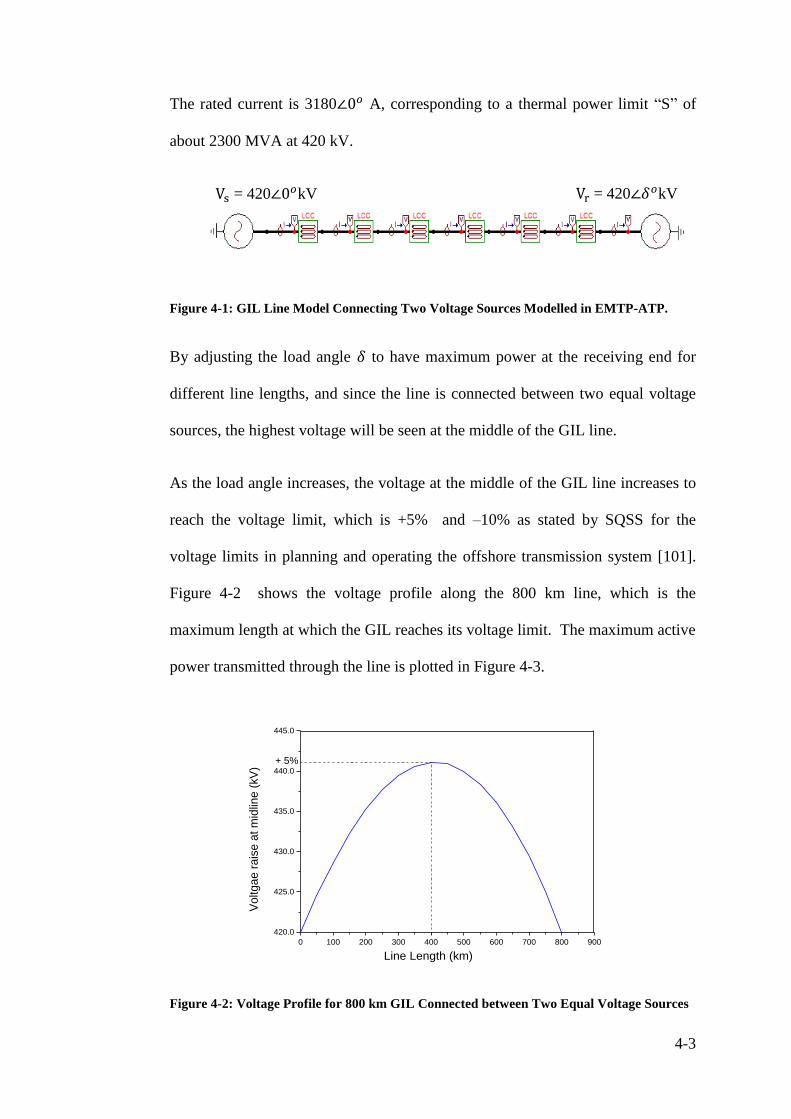
4-3

The rated current is 3180∠0𝑜 A, corresponding to a thermal power limit “S” of

about 2300 MVA at 420 kV.

Figure 4-1: GIL Line Model Connecting Two Voltage Sources Modelled in EMTP-ATP.

By adjusting the load angle 𝛿 to have maximum power at the receiving end for

different line lengths, and since the line is connected between two equal voltage

sources, the highest voltage will be seen at the middle of the GIL line.

As the load angle increases, the voltage at the middle of the GIL line increases to

reach the voltage limit, which is +5% and –10% as stated by SQSS for the

voltage limits in planning and operating the offshore transmission system [101].

Figure 4-2 shows the voltage profile along the 800 km line, which is the

maximum length at which the GIL reaches its voltage limit. The maximum active

power transmitted through the line is plotted in Figure 4-3.

Figure 4-2: Voltage Profile for 800 km GIL Connected between Two Equal Voltage Sources

0 100 200 300 400 500 600 700 800 900

420.0

425.0

430.0

435.0

440.0

445.0

Voltga

e r

ais

e a

t m

idlin

e (

kV

)

Line Length (km)

+ 5%

Vs = 420∠0𝑜kV Vr = 420∠𝛿𝑜kV

4-4

Figure 4-3: Maximum Active Power Transmitted through the GIL Line versus Line Length

for 800 km GIL Connected between two Equal Voltage Sauces

It can be seen from Figure 4-3 that the maximum active power transmitted

through the line decreases as the line length increases, up to about 800 km where

the voltage limit +5% has been reached at the middle of the GIL line. It can be

seen also that the GIL can carry active power of up to 2070 MW, which equates

to 90% of its thermal power rating for distances of up to 680 km without any

shunt reactive power compensation; this demonstrates the high transmission

capability of GIL.

4.2.1. Comparison of Maximum Transmission Capacity with

other AC Transmission Technology

The production of a large amount of reactive power is the main limitation factor

for utilizing HVAC transmission systems over long distances. This can be

mitigated by installing reactive compensation at both ends of the transmission

line. Increasing the line length beyond this distance requires additional shunt

compensation to be installed at the middle of the line length. In an offshore

application, it is very expensive to install shunt compensation at the middle of the

0 100 200 300 400 500 600 700 800 900

2000

2050

2100

2150

2200

2250

2300

PM

AX (

MW

)

Line Length (km)

90 %

4-5

line as it requires additional offshore platforms; therefore, economic transmission

distances are limited [102], [103].

A comparison study for maximum real power transmission against line length has

been made between three different AC transmission systems, with each of the

three AC transmission systems transmitting its maximum thermal power limit

XLPE cable, overhead line, and GIL, all of them operating at 420 kV.

Long XLPE cables and overhead lines require permanently connected inductive

shunt compensation, in order to suppress undesired effects of their reactive power

output. Therefore, 50/50% inductive shunt reactors were installed at both

terminals for XLPE cable and overhead line to compensate their reactive power

output. No reactive power compensation is used for the GIL line. Figure 4-4

shows a comparison of maximum real power transfer for the different

transmission systems.

Figure 4-4: Comparison of Maximum Real Power Transfer for Uncompensated 420kV GIL

Transmission Line with 50/50 Compensated Overhead Line and XLPE Cable Transmitting

their Thermal Power Limit versus Line Length.

As can be seen in Figure 4-4, even though the GIL line is operating without

reactive power compensation a big difference is evident between the GIL and

0 100 200 300 400 500 600 700 800 900

0

500

1000

1500

2000

2500

GIL

Overhead Line

XLPE Cable

PM

AX

(M

W)

Line Length (km)

90 %

90 %

4-6

other AC transmission technologies in both the amount of real power that can be

transmitted and in the distances. The reason for this is the large cross section of

the GIL conductor, which allows transmission of a high amount of real current. At

the same time, the reactive current generated by the line capacitance is still small

and will not reach the amount of real current transmitted by the GIL even with an

increase in the line length.

In the case of XLPE cable, Figure 4-4 shows that the critical distance is achieved

before the voltage drop limit. When the reactive current produced by the cable

reaches the nominal current at the end of the cable, there is no transmission

capacity left for active power transmission; this is called the critical line length

[104]. For the considered cable, the critical distance is achieved at 200 km. It can

be seen also that 90% of the thermal rated power was reached at about 85 km with

50/50 shunt reactive power compensation connected at both ends.

For the considered overhead line, the voltage drop limit was reached before the

critical line length was reached. It can be seen that the voltage drop limit was

reached at 435 km and 90% of the thermal rated power was reached at about 280

km also with 50/50 shunt reactive power compensation connected at both ends.

4.3. Electrical Transmission Characteristics for GIL under

Different Line Lengths

In this section, the effect of the line length on electrical transmission

characteristics for a 100% load condition and a 0.8 typical power factor is studied.

A computer model was developed using EMTP-ATP to quantify the voltage,

current and power transfer characteristics for different line lengths. In addition, an

4-7

analytical method using MATLB was used to calculate the voltage, current and

power profiles for GIL line lengths ranging from 200 km to 500 km.

4.3.1. EMTP Simulation Model

The GIL is represented by three single-core GIL lines using a 𝜋 model. It is

divided into sections of 50 km length each. Figure 4-5 shows a GIL model

constructed in EMTP-ATP and an assumed sending end voltage of Vs =

420∠0𝑜kVrms. In order to achieve the thermal current limit 3180A at the

receiving end with a power factor of 0.8, the load at the end of line was specified

as given in Table 4-1. The voltage and current profiles are plotted in Figure 4-6

(a) and (b) respectively and the corresponding real and reactive powers are plotted

in Figure 4-6 (c) and (d).

Figure 4-5: GIL Model in EMTP Sectionalized to 50 km each Connected by Load Operating

at 0.8 Power Factor.

Table 4-1: Load Connected to the End of Each Line Operating at 0.8 Power Factor

Line Length (km) ZLoad (Ω)

200 55 + j 39.9

300 52 + j 38

400 49.35 + j 36.3

500 47+ j 34.54

Vs = 420∠0𝑜kV

Cos (𝜑) = 0.8

4-8

(a) Voltage Drop Profiles

(b) Current Rise profiles

(c) Real Power Losses Profiles

(d) Reactive Power Gain Profiles

Figure 4-6: EMTP-ATP Simulation Results for Electrical Transmission Characteristics of

Different GIL Line Lengths Ranging from 200 km to 500 km.

4.3.2. Analytical Method

The analytical method was based on the long transmission line equations that are

used to calculate the voltage, current and power profiles for different GIL line

lengths [105]. The total series impedance Z and the total shunt admittance Y per

phase are calculated based on the per unit line length parameters shown in Table

3-2, and their values are shown in Table 4-2 together with the characteristic

impedance, propagation constant, and surge impedance loading.

0 100 200 300 400 500

3.0

3.2

3.4

3.6

3.8

4.0

4.2

4.4

4.6

Pea

k P

hase C

urr

ent (k

A)

Line Length (km)

200 km 300 km 400 km 500 km

(b)

0 100 200 300 400 500

480.0

500.0

520.0

540.0

560.0

580.0

Pea

k R

eal P

ow

er

Per

Pha

se

(M

W)

Line Length (km)

(c)

200 km

300 km

400 km

500 km

0 100 200 300 400 500

150.0

200.0

250.0

300.0

350.0

400.0

Pe

ak R

ea

ctive

Po

we

r P

er

Ph

ase

(M

Va

r)

Line Length (km)

200 km

300 km

400 km

500 km

(d)

0 100 200 300 400 500

260.0

280.0

300.0

320.0

340.0

Pea

k P

hase V

oltage (

kV

)

Line Length (km)

200 km

300 km

400 km

500 km

(a)

4-9

Table 4-2: The Electrical GIL Line Parameters Used in the Analytical Method.

Longitudinal impedance Z= r + jωl mΩ/km 8.616+j64

Shunt admittance Y= g + jωc mS/km 0 + j0.017

Characteristic Impedance Z0= √Z/Y Ω 61.64 - j 4.1

Propagation Constant γ = √Z*Y 1/km 0.0001 + j0.001

Surge Impedance Loading

at 420 kV

SIL= (420kV)2/Z0 MVA 2893.6

The ABCD generalised circuit constants were obtained using the electrical

parameters shown in Table 4-2 The relationship between the sending and

receiving end quantities given in Equations (4-1) and (4-2) were adopted

assuming a maximum sending end voltage of Vs = 420∠0𝑜kVrms, a maximum

receiving end current as determined from the EMTP simulation method shown in

Table 4-3, and a power factor of 0.8 at the receiving end. The MATLAB

equations are shown in Appendix 5.

𝑉𝑅 = 𝐴 ∗ 𝑉𝑠 − 𝐵 ∗ 𝐼𝑆 (4-1)

𝐼𝑅 = 𝐷 ∗ 𝐼𝑆 − 𝐶 ∗ 𝑉𝑆 (4-2)

Table 4-3: Maximum Sending End Current as Determined from the EMTP-ATP Simulation

Model.

Line Length (km) Sending End Current (A)

200 3145∠20.9o

300 3361∠24.90

400 3611∠28.20

500 3882∠310

4-10

Figure 4-7 (a) and (b) respectively show the calculated voltage and current

profiles along the GIL. The active and reactive power flow can be calculated at

any point along the GIL using Equations (4-3) and (4-4). Figure 4-7 (c) and (d)

respectively show calculated active and reactive power flows on the line where

(θV – θI) is the angle by which the current is lagging the voltage.

𝑃𝑅 = 𝑉𝑅 ∗ 𝐼𝑅 ∗ Cos (θV – θI) (4-3)

𝑄𝑅 = 𝑉𝑅 ∗ 𝐼𝑅 ∗ Sin (θV – θI) (4-4)

(a) Voltage Drop Profiles

(c) Real Power Losses profiles

(b) Current Rise profiles

(d) Reactive Power Gain Profiles

Figure 4-7: MATLAB Calculation Results for Electrical Transmission Characteristics of

Different GIL Line Lengths Ranging from 200 km to 500 km.

0 100 200 300 400 500 600

2.6

2.7

2.8

2.9

3

3.1

3.2

3.3

3.4

3.5x 10

5

Line Length (km)

Pe

ak P

ha

se

Vo

lta

ge

(kV

)

0 100 200 300 400 500 6006.6

6.8

7

7.2

7.4

7.6

7.8

8

8.2x 10

8

Line Length (km)

Pe

r P

ha

se

Pe

ak R

ea

l P

ow

er

(MW

)

0 100 200 300 400 500 6003000

3200

3400

3600

3800

4000

4200

4400

4600

4800

Line Length (km)

Pe

ak P

ha

se

Cu

rre

nt (A

)

0 100 200 300 400 500 6002.5

3

3.5

4

4.5

5

5.5

6x 10

8

Line Length (km)

Pe

r P

ha

se

Pe

ak R

ea

ctive

Po

we

r (M

Va

r)

200 km

300 km

400 km

500 km

200 km 300 km 400 km 500 km

200 km

300 km

400 km

500 km

200 km 300 km

400 km

500 km

4-11

4.3.3. Comparison of Simulation and Analytical Results

The electrical power transfer characteristics of GIL have been studied for lengths

ranging from 200 km to 500 km. The electrical power transfer characteristics

were calculated using Equation (4-5).

% = (𝑅𝑒𝑐𝑒𝑖𝑣𝑖𝑛𝑔 𝑒𝑛𝑑

𝑠𝑒𝑛𝑑𝑖𝑛𝑔 𝑒𝑛𝑑− 1)*100 (4-5)

A summary of the results obtained is given in Table 4-4. As can be observed, the

results of the analytical model agree very closely with the results obtained from

the EMTP-ATP simulation method.

Table 4-4: Electrical Power Transfer Characteristics of GIL for Length Ranging from 200

km to 500 km.

Line Length

(km)

Voltage Drop

ΔV (%)

Current Rise

I (%)

Real Power Losses P

P (%)

Reactive Power Gain

Q (%)

200 -11 +13.9 -2.48 +17.4

300 -15.64 +19.9 -3.33 +30.87

400 -19.81 +25.3 -4.41 +50

500 -23.58 +43.5 -5.6 +82

The voltage profiles along the GIL are shown in Figure 4-6 (a) (EMTP) and

Figure 4-7 (a) (analytical equations) for line lengths ranging from 200 km to 500

km. From the figures, it can be seen that there is a fall in the voltage from the

sending to the receiving end. The voltage drop percentage increased from -11%

for 200 km to -23.58% for 500 km. The voltage drop percentages fall outside of

the voltage drop limit + 5% and – 10% stated by SQSS for voltage limits in

planning and operating the offshore transmission system [101].

The voltage drop percentage for each line length with this load condition is due to

the heavy inductive load. Therefore, in order to maintain the load bus voltage

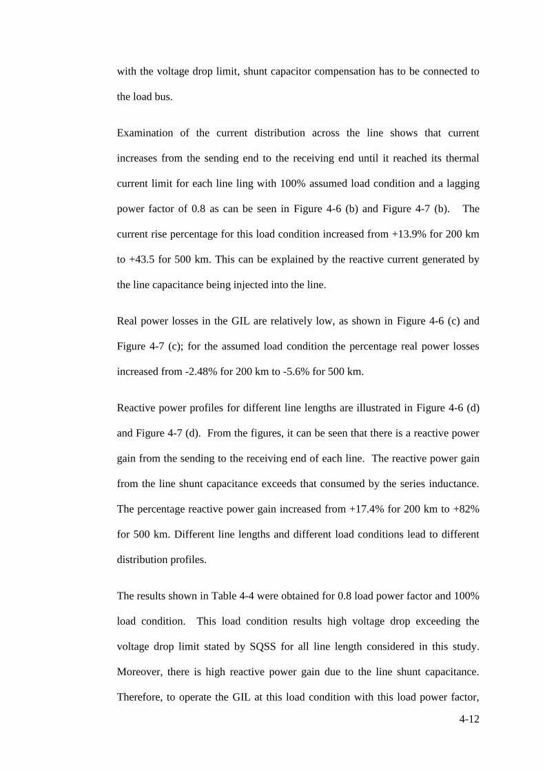
4-12

with the voltage drop limit, shunt capacitor compensation has to be connected to

the load bus.

Examination of the current distribution across the line shows that current

increases from the sending end to the receiving end until it reached its thermal

current limit for each line ling with 100% assumed load condition and a lagging

power factor of 0.8 as can be seen in Figure 4-6 (b) and Figure 4-7 (b). The

current rise percentage for this load condition increased from +13.9% for 200 km

to +43.5 for 500 km. This can be explained by the reactive current generated by

the line capacitance being injected into the line.

Real power losses in the GIL are relatively low, as shown in Figure 4-6 (c) and

Figure 4-7 (c); for the assumed load condition the percentage real power losses

increased from -2.48% for 200 km to -5.6% for 500 km.

Reactive power profiles for different line lengths are illustrated in Figure 4-6 (d)

and Figure 4-7 (d). From the figures, it can be seen that there is a reactive power

gain from the sending to the receiving end of each line. The reactive power gain

from the line shunt capacitance exceeds that consumed by the series inductance.

The percentage reactive power gain increased from +17.4% for 200 km to +82%

for 500 km. Different line lengths and different load conditions lead to different

distribution profiles.

The results shown in Table 4-4 were obtained for 0.8 load power factor and 100%

load condition. This load condition results high voltage drop exceeding the

voltage drop limit stated by SQSS for all line length considered in this study.

Moreover, there is high reactive power gain due to the line shunt capacitance.

Therefore, to operate the GIL at this load condition with this load power factor,

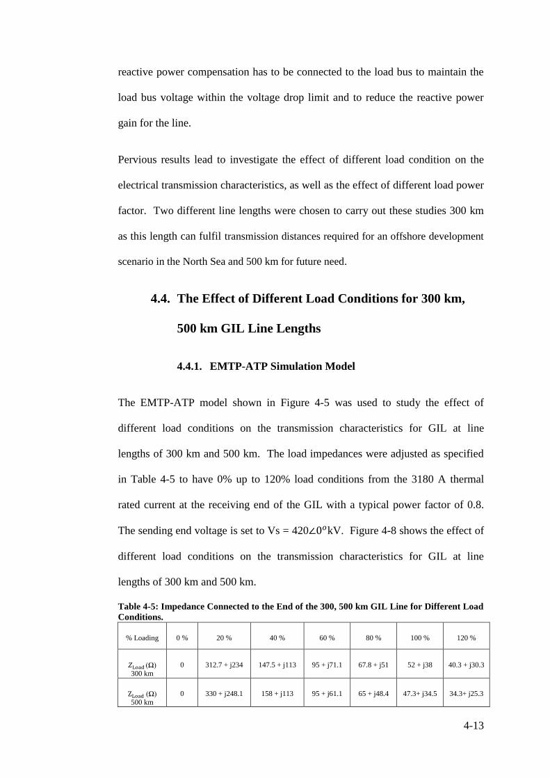
4-13

reactive power compensation has to be connected to the load bus to maintain the

load bus voltage within the voltage drop limit and to reduce the reactive power

gain for the line.

Pervious results lead to investigate the effect of different load condition on the

electrical transmission characteristics, as well as the effect of different load power

factor. Two different line lengths were chosen to carry out these studies 300 km

as this length can fulfil transmission distances required for an offshore development

scenario in the North Sea and 500 km for future need.

4.4. The Effect of Different Load Conditions for 300 km,

500 km GIL Line Lengths

4.4.1. EMTP-ATP Simulation Model

The EMTP-ATP model shown in Figure 4-5 was used to study the effect of

different load conditions on the transmission characteristics for GIL at line

lengths of 300 km and 500 km. The load impedances were adjusted as specified

in Table 4-5 to have 0% up to 120% load conditions from the 3180 A thermal

rated current at the receiving end of the GIL with a typical power factor of 0.8.

The sending end voltage is set to Vs = 420∠0𝑜kV. Figure 4-8 shows the effect of

different load conditions on the transmission characteristics for GIL at line

lengths of 300 km and 500 km.

Table 4-5: Impedance Connected to the End of the 300, 500 km GIL Line for Different Load

Conditions.

% Loading 0 % 20 % 40 % 60 % 80 % 100 % 120 %

𝑍Load (Ω) 300 km

0 312.7 + j234 147.5 + j113 95 + j71.1 67.8 + j51 52 + j38 40.3 + j30.3

ZLoad (Ω) 500 km

0 330 + j248.1 158 + j113 95 + j61.1 65 + j48.4 47.3+ j34.5 34.3+ j25.3

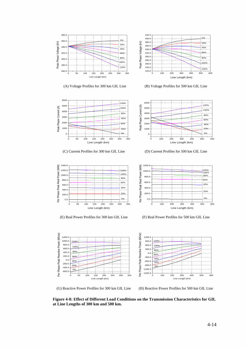
4-14

(A) Voltage Profiles for 300 km GIL Line

(B) Voltage Profiles for 500 km GIL Line

(C) Current Profiles for 300 km GIL Line

(D) Current Profiles for 500 km GIL Line

(E) Real Power Profiles for 300 km GIL Line

(F) Real Power Profiles for 500 km GIL Line

(G) Reactive Power Profiles for 300 km GIL Line

(H) Reactive Power Profiles for 500 km GIL Line

Figure 4-8: Effect of Different Load Conditions on the Transmission Characteristics for GIL

at Line Lengths of 300 km and 500 km.

0 50 100 150 200 250 300 350260.0

280.0

300.0

320.0

340.0

360.0

380.0

Peak

Pha

se V

olta

ge (

kV)

Line Length (km)

0%

20%

40%

60%

80%

100%

120%

0 100 200 300 400 500 600220.0

240.0

260.0

280.0

300.0

320.0

340.0

360.0

380.0

400.0

420.0

Pea

k P

hase

Vol

tag

e (k

V)

Line Length (km)

0%

20%

40%

60%

80%

100%

120%

0 50 100 150 200 250 300 350

0

1000

2000

3000

4000

5000

6000

Peak

Pha

se C

urr

ent

(A)

Line Length (km)

120%

100%

80%

60%

40%

20%

0%

0 100 200 300 400 500 600

0

1000

2000

3000

4000

5000

6000

Pea

k P

hase

Cur

rent

(A

)Line Length (km)

120%

100%

80%

60%

40%

20%

0%

0 50 100 150 200 250 300 350

0.0

200.0

400.0

600.0

800.0

1000.0

1200.0

1400.0

Per

Ph

ase

Pe

ak

Rea

l Pow

er

(MW

)

Line Length (km)

120%

100%

80%

60%

40%

20%

0%

0 100 200 300 400 500 600

0.0

200.0

400.0

600.0

800.0

1000.0

1200.0

Per

Pha

se P

eak

Rea

l Pow

er (

MW

)

Line Length (km)

120%

100%

80%

60%

40%

20%

0%

0 50 100 150 200 250 300 350

-600.0

-400.0

-200.0

0.0

200.0

400.0

600.0

800.0

1000.0

1200.0

Per

Pha

se P

eak

Rea

ctiv

e P

ower

(M

Var

)

Line Length (km)

120%

100%

80%

60%

40%

20%

0%

0 100 200 300 400 500 600-1500.0

-1200.0

-900.0

-600.0

-300.0

0.0

300.0

600.0

900.0

1200.0

Per

Pha

se P

eak

Rea

ctiv

e P

ower

(M

Var

)

Line Length (km)

120%

100%

80%

60%

40%

20%

0%

4-15

The electrical power transfer characteristics of 300 km and 500 km GIL have

been studied for different load conditions. Figure 4-8 (A, B) show the voltage

profiles for both line lengths. It can be seen from the figures that the highest

voltage were seen at the receiving ends are at 0% load condition which is +5.44%

for 300 km and +16.4% for 500 km.

By increasing the load from 20% up to 120%, the voltage continues dropping

until it reaches -20.4% voltage drop for 300 km and -32.9% voltage drop for 500

km for 120% load condition and 0.8 power factor.

It should be noted that during the change in the voltage from the case of no load

condition to the 120% load condition, the voltage crosses the voltage drop limit

+5% and -10%, but at very low load conditions, which are considered non-

economic load conditions to operate such a transmission line. Table 4-6 shows

the voltage drop at the receiving end of GIL line lengths of 300 km and 500 km

for different load conditions.

Table 4-6: Voltage Drop at the Receiving End of 300 km and 500 km GIL Line Lengths for

Different Loads.

Length (km) 0 % 20 % 40 % 60 % 80 % 100 % 120 %

300 + 5.44% + 1.57% - 2.6% - 6.708% - 11.1% -15.63% - 20.4%

500 + 16.4% + 9.2% + 2.05% - 6.3% -1 4.7% - 23.28% - 32.9%

Figure 4-8 (C, D) show the current profiles for different load conditions. It can be

seen that for the case of no load condition, there is no current flow through the

line at the receiving end. By increasing the load from 20% to 120%, the current

starts increasing from the sending end to the receiving end due to the reactive

current generated by the line capacitance until it reaches 18.7% for 300 km and

4-16

40% for 500 km at a 120% load condition and a 0.8 power factor. Table 4-7

shows the current increase at the receiving end of GIL line length of 300 km and

500 km for different load conditions.

Table 4-7: Current Rise at the Receiving End for 300 km and 500 km GIL Line Lengths.

Length (km) 0 % 20 % 40 % 60 % 80 % 100 % 120 %

300 0% -36.7% 19.3% 31.4% 27.6% 20.3% 18.7%

500 0% -66% -22.9% 19.7% 48.4% 43.1% 40.1%

The real power profiles are shown in Figure 4-8 (E, F). It can be seen that the real

power losses are relatively low; even for a 120% load condition and a 0.8 power

factor, the power losses are 4.5% for a line length of 300 km and 7.7% for 500

km, which confirms that the power losses are very low in the GIL transmission

line. Table 4-8 shows the real power losses at the receiving end of the 300 km

and 500 km GIL for different load conditions.

Table 4-8: Real Power Losses at Receiving End of 300 km and 500 km GILs.

Length (km) 0 % 20 % 40 % 60 % 80 % 100 % 120 %

300 0% 0.8% 1.1% 1.7% 2.5% 3.4% 4.5%

500 0% 2.1% 2.29% 2.51% 3.86% 5.54% 7.75%

The reactive power profiles are shown in Figure 4-8 (G, H). It can be seen that

there is an increase in the reactive power from the sending end to the receiving

end for every load condition at a 0.8 power factor, except for the 120% load

condition.

The highest increase in the reactive power is at the 60% load condition with

355%, which is the worst load condition for 300 km. For 500 km, the worst load

4-17

condition was seen at the 80% load condition, with a 213% increase in the

reactive power.

For the 120% load condition, the big inductive load connected at the receiving

end absorbs all the reactive power generated by the line capacitance. The reactive

power generated by the line capacitance is not enough to feed this inductive load.

Therefore, the reactive power starts decreasing at the receiving end for both line

lengths.

Table 4-9 shows the reactive power at the receiving end of the 300 km and 500

km GILs. Table 4-9 shows that when the GIL is fully loaded, the increase in

reactive power at the receiving end is reduced to lower levels.

Table 4-9: Reactive Power at Receiving End of the 300 km and 500 km GILs.

Length (km) 0% 20% 40% 60% 80% 100% 120%

300 0% 145% 279% 355% 108% 31% -0.8%

500 0% 123% 160.5% 183% 213% 83% -2.9%

4.5. Effect of variation in Receiving End Power Factor on

Transmission Performance for a 300 km and 500 km

GIL Lengths

4.5.1. Effect of Lagging Power Factors on Transmission

Performance

In this section, the effect of different lagging power factors on the transmission

characteristics has been studied for 300 km and 500 km GIL line lengths. The

4-18

EMTP model shown in Figure 4-5 was used, and the sending end voltage was set

to Vs = 420∠0𝑜kV.

Different inductive loads were adjusted at the receiving end to achieve a load of

3180A, which represents a 100% load condition. The loads connected at the

receiving end of GIL as a function of the lagging power factors are shown in

Table 4-10. Figure 4-9 shows the effect of the lagging power factors on the

transmission performance of 300 km and 500 km GILs.

Table 4-10: Load Connected to the Lines End for Different Lagging Power Factors

Power factor Z load (Ω) for 300 km Z load (Ω) for 500 km

Unity 77.31 + j0 87.57 + j0

0.98 69.75 + j14.13 68 + j13.424

0.95 65.5 + j21.67 62.5 + j20.41

0.9 60 + j29.52 56.5 + j26.69

0.8 52 + j37.994 47.3 + j34.54



0 50 100 150 200 250 300 350 400285.0

300.0

315.0

330.0

345.0

Pe

ak P

ha

se V

olta

ge

(kV

)

Line Length (km)

Cos ()

Cos ()

Cos )

Cos ()

Cos ()

(A)

-10%

0 100 200 300 400 500 600

260.0

280.0

300.0

320.0

340.0

360.0

Cos ()

Peak P

ha

se

Voltag

e (

kV

)

Line Length (km)

Cos ()

Cos ()

Cos ()

Cos ()

-10 %

(B)

4-19







Figure 4-9: Effect of Different Lagging Power Factors on Electrical Transmission

Characteristics for 300 km and 500 km GIL Line Lengths.

The relationship between the voltage drop and the different lagging power factors

for both line lengths is shown in Figure 4-9 (A, B). From the voltage profile of

300 km, it can be seen that there is drop in the voltage from the sending end to the

receiving end. This drop increased from -1.2% for a unity power factor to a -

15.45% voltage drop for a 120% load condition and a 0.8 lagging power factor.

0 50 100 150 200 250 300 350

3600

3800

4000

4200

4400

4600

Cos()

Cos()

Cos()

Cos()

Peak

Pha

se C

urr

ent

(A)

Line Length (km)

Cos()

0 100 200 300 400 500 6003000

3200

3400

3600

3800

4000

4200

4400

4600

4800

Cos()

Cos()

Cos()

Cos()

Peak

Pha

se C

urr

ent

(A)

Line Length (km)

Cos()

0 100 200 300 400500.0

550.0

600.0

650.0

700.0

750.0

800.0

Per

Ph

ase P

eak R

ea

l pow

er

(MW

)

Line Length (km)

Cos ()

Cos ()

Cos ()

Cos ()

Cos ()

(F)

0 100 200 300 400 500 600450.0

500.0

550.0

600.0

650.0

700.0

750.0

800.0

Pe

r P

ha

se P

ea

k R

ea

l Po

we

r (M

W)

Line Length (km)

Cos ()

Cos ()

Cos ()

Cos ()

Cos ()

(G)

0 100 200 300 400

-100.0

0.0

100.0

200.0

300.0

400.0

500.0

Pe

r P

ha

se P

ea

k R

ea

ctiv

e P

ow

er

(MV

ar)

Line Length (km)

Cos ()

Cos ()

Cos ()

Cos ()

Cos ()

(H)

0 100 200 300 400 500 600-300.0

-200.0

-100.0

0.0

100.0

200.0

300.0

400.0

500.0

Per

Ph

ase

Pe

ak

Rea

ctiv

e P

ow

er

(MV

ar)

Line Length (km)

Cos ()

Cos ()

Cos ()

Cos ()

Cos ()

(I)

4-20

According to the voltage drop limit stated by SQSS, which is +5% and -10% for

planning and operating offshore transmission systems [101], 300 km GIL can be

operated as an offshore transmission system with a lagging power factor limit

between unity and 0.95 without the need for any reactive power compensation

support at the load bus.

For 500 km, the drop in the voltage increases from +2.4% for a unity power factor

to -23.4% for a 0.8 lagging power factor. From the voltage profiles, it can be seen

that the limit of the lagging power factor to operate the 500 km GIL as an

offshore transmission system without the need for any reactive power

compensation support is between unity and 0.98. Table 4-11 shows the voltage

drop at the receiving end of 300 km and 500 km due to the variation in the

lagging power factors.

Table 4-11: Voltage Drop at Receiving End of 300 km and 500 km for Different Lagging

Power Factors.

Length (km) Cos (φ) = 1 Cos (φ) = 0.98 Cos (φ) = 0.95 Cos (φ) = 0.9 Cos (φ) = 0.8

300 -1.2% -4.9% -9.2% -12% -15.45%

500 2.4% -8.78% -13.7% -17.2% -23.4%

Figure 4-9 (C, D) show the current distribution profiles for both line lengths. It

can be seen that for a unity power factor, there is a 2.9% loss in the current flow

from the sending end to the receiving end for the 300 km line length, which

means that the real current flows through a mostly resistive impedance.

For other power factors, it can be seen that there is an increase in the current from

the sending end to the receiving end. This increase starts from +3.26% for a 0.98

4-21

lagging power factor to +20.62% for a 0.8 lagging power factor due to the

reactive current generated by the line capacitance.

For 500 km GIL line length at a unity power factor, there is a loss in the current

from the sending to the receiving end of -10.88%. For a 0.98 lagging power

factor, the current increases from +7.67% to +43.1% for a 0.8 lagging power

factor as shown in Table 4-12.

Table 4-12: Current Gain at Receiving End of 300 km and 500 km for Different Lagging

Power Factors.


300 -2.56% 3.26% 10.59% 16.28% 20.62%

500 -10.88% 7.76% 15.5% 26% 43.1%

The real power profiles for the 300 km and 500 km line lengths are shown in

Figure 4-9 (E, F). It can be seen that the percentage real power losses are

relatively low; even for 500 km and a 0.8 power factor, the power losses are

5.5%. The figures show the effect of the variation in power factors on the amount

of real power that can be transmitted through the GIL. Table 4-13 shows the real

power losses for the different lagging power factors for both line lengths.

Table 4-13: Real Power Losses for Different Lagging Power Factors for 300 km and 500 km

GILs.


300 2.88% 2.95% 3.05% 3.016% 3.31%

500 4.47% 4.89% 4.91% 4.97% 5.55%

4-22

The reactive power profiles along the 300 km and 500 km lines GIL are shown in

Figure 4-9 (G, H). For the 300 km line, it can be seen that for unity power factor,

the reactive power received at the receiving end is zero.

For the remaining power factors considered here, it can be seen that there are

positive reactive power flows out from both ends of the GIL line, which means

there is a demand for capacitive reactive power compensation. The reactive

power demand is decreased by reducing the power factor, which means increasing

the line capacitance. Even though there is a high demand for capacitive reactive

power compensation, the voltage at the load bus is still within the voltage drop

limit from 0.95 lagging up to unity power factor.

For 500 km, it can be seen that the demand for capacitive reactive power

compensation increases as the line length increases. The power factor operating

limit decreases between 0.98 and unity power factor. Table 4-14 shows the

reactive power demand for different lagging power factors for 300 km and 500

km GIL.

Table 4-14: Reactive Power Demand for Different Lagging Power Factors for 300 km and

500 km GIL.


300 0% +180% +72% +45% +31%

500 0% +700% +280.5% +161.4% +82.3%

4-23

4.5.2. Effect of Leading Power Factors on Transmission

Performance

In this section, the effect of different leading power factors on the transmission

characteristics is investigated for 300 km and 500 km GIL line lengths. Different

capacitive loads are adjusted at the receiving end to achieve a load of no more

than 3180 A, which represents a 100% load condition.

The loads connected at the receiving end of the GIL as a function of the leading

power factors are shown in Table 4-15. Figure 4-10 shows the effect of leading

power factors on the transmission performance of 300 km and 500 km GIL line

lengths.

Table 4-15: Load Connected to the Line End for Different Leading Power Factors.

Power factor Z load (Ω) for 300 km Z load (Ω) for 500 km

Unity 77.31 – j0 87.57 – j0

0.98 88.25 – j0.0568 127 – j0.03925

0.95 93.5 – j0.0327 152.75 – j0.0201

0.9 97.5 – j0.0214 176 – j0.01224

0.8 98 – j0.01365 204 – j0.00659



0 100 200 300 400

315.0

330.0

345.0

360.0

375.0

390.0

405.0

Pe

ak P

ha

se

Vo

lta

ge

(kV

)

Line Length (km)

+ 5%

Cos ()

Cos ()

Cos ()

Cos ()

Cos ()

(A)

0 100 200 300 400 500 600330.0

345.0

360.0

375.0

390.0

405.0

420.0

435.0

450.0

Pe

ak P

ha

se

Vo

lta

ge

(kV

)

Line Length (km)

+ 5%

Cos ()

Cos ()

Cos ()

Cos ()

Cos ()

(B)

4-24







Figure 4-10: Effect of Different Leading Power Factors on Electrical Transmission

Characteristics for 300 km and 500 km GIL Line Lengths.

Leading power factors cause an increase in the voltage from the sending end to

the receiving end of the line, as shown in Figure 4-10 (A, B). For 300 km, the

increase in the voltage starts from -1.2% for unity power factor to +14% for 0.8

leading power factor.

0 100 200 300 4003000

3200

3400

3600

3800

4000

4200

4400

4600

Pe

ak P

ha

se

Cu

rre

nt

(A)

Line Length (km)

Cos ()

Cos ()

Cos ()

Cos ()

Cos ()

(C)

0 100 200 300 400 500 6001500

2000

2500

3000

3500

4000

4500

5000

Pe

ak P

ha

se C

urr

en

t (A

)

Line Length (km)

Cos ()

Cos ()

Cos ()

Cos ()

Cos ()

(D)

0 100 200 300 400

500.0

550.0

600.0

650.0

700.0

750.0

800.0

Pe

r P

ha

se P

ea

k R

ea

l Po

we

r (M

W)

Line Length (km)

Cos )

Cos )

Cos )

Cos )

Cos )

(F)

0 100 200 300 400 500 600200.0

300.0

400.0

500.0

600.0

700.0

800.0

Pe

r P

ha

se P

ea

k R

ea

l Po

we

r (M

W)

Line Length (km)

Cos )

Cos )

Cos )

Cos )

Cos )

(G)

0 100 200 300 400-700.0

-600.0

-500.0

-400.0

-300.0

-200.0

-100.0

0.0

100.0

200.0

Pe

r P

ha

se P

ea

k R

ea

ctiv

e P

ow

er

(MV

ar)

Line Length (km)

Cos ()

Cos ()

Cos ()

Cos ()

Cos ()

(H)

0 100 200 300 400 500 600

-700.0

-600.0

-500.0

-400.0

-300.0

-200.0

-100.0

0.0

100.0

200.0

Per

Ph

ase

Pe

ak

Rea

ctiv

e P

ow

er

(MV

ar)

Line Length (km)

Cos ()

Cos ()

Cos ()

Cos ()

Cos ()

(I)

4-25

For 500 km, the increase in the voltage is increased from +2.4% for unity power

factor to +24.5% for a 0.8 leading power factor. Table 4-16 shows the voltage

drop at the receiving end of the 300 km and 500 km lines for different leading

power factors.

The voltage drop limit stated by SQSS for planning and operating offshore

transmission systems is +5% and -10%. Table 4-16 shows that the operating

power factor ranges from unity to a 0.98 leading power factor for the 300 km line

length, where the voltage at the load bus falls within the voltage drop limit, which

is +5%. For the 500 km line length, the voltage increase falls out of the voltage

drop limit except for unity power factor.

Table 4-16: Voltage Drop at Receiving End of 300 km and 500 km for Different Leading

Power Factors.

Length (km) Cos (φ) = 1 Cos (φ) = -0.98 Cos (φ) = -0.95 Cos (φ) = -0.9 Cos (φ) = -0.8

300 -1.2% 4.55% 7.6% 10.5% 14%

500 2.4% 14.1% 18.5% 21.5% 24.5%

Operating GIL with leading power factor will lead to the highest current being

seen at the sending end as shown in Figure 4-10 (C, D). For the 300 km line

length, the current losses increased from the sending end to the receiving end by -

2.65% for unity power factor to -29% for a 0.8 leading power factor. For the 500

km line length, the current losses increased from the sending end to the receiving

end by -10.88% for unity power factor to -62.7% for a 0.8 leading power factor as

shown in Table 4-17.

4-26

Table 4-17: Current Losses at Receiving End of 300 km and 500 km for Different Lagging

Power Factors.


300 -2.56% -11.45% -16.6% -22% -29%

500 -10.88% -32.89% -43.5% -52.3% -62.7%

The real power profiles for the 300 km and 500 km line lengths operated at

different leading power factors are shown in Figure 4-10 (E, F). Table 4-18

shows real power losses at the receiving ends of both line lengths. It can be seen

that the percentage real power losses is relatively low even for the 500 km line

length where the power loss is 5.5% at a 0.8 leading power factor.

Table 4-18: Real Power Losses for Different Leading Power Factors for 300 km and 500 km

GIL.


300 2.88% 2.8% 2.81% 2.9% 3.3%

500 4.47% 4.5% 4.7% 4.9% 5.5%

The reactive power profiles are shown in Figure 4-10 (G, H) for leading power

factors. It can be seen that the percentage of the reactive power gain decreases by

the decreasing leading power factor from -49.5% for a 0.98 leading power factor

to -34.7% for a 0.8 leading power factor for the 300 km line length.

For the 500 km line length, the reactive power gain decreases from -75.8% for a

0.98 leading power factor to -69.8% for a 0.8 leading power factor. Table 4-19

shows the reactive power gain for different leading power factors at the receiving

ends for both line lengths. It should be noted that the reactive power gain in the

4-27

case of a leading power factor is smaller than the reactive power gain in the case

of a lagging power factor due to the local capacitive reactive power supply at the

load bus.

Table 4-19: Reactive Power Gain for Different Leading Power Factors for 300 km and 500

km GIL line lengths


300 0% -49.5% -42% -37.9% -34.7%

500 0% -75.8% -72.2% -70.7% -69.8%

4.6. Summary

AC transmission technologies such as overhead line and XLPE cable are limited

in their transmission capacity and transmission distances. The main reason for

this limit is their high shunt capacitance. As the length of the AC transmission

system increases, the capacitive charging current increases; this, in turn, reduces

the ability to transmit real power and causes a voltage drop at the load bus.

Shunt reactive power compensation has to be connected to the load bus to

regulate the voltage within acceptable voltage drop limit and to transmit more real

power for these transmission technologies.

This limit for utilizing AC transmission technologies for long distances without

any need for reactive power compensation can be addressed by introducing GIL

as a transmission system. GIL has lower shunt capacitance than XLPE cable by

four times which make the reactive power generated by the GIL shunt capacitance

less by four times than the reactive power generated by XLPE cable for the same

voltage level. The high amount of real power that can be transmitted by a single

4-28

circuit of GIL is another advantage of utilizing GIL over other underground or

submarine transmission technology.

The effects of different factors on the transmission characteristics, such as line

length, load conditions, and variable power factors, have been studied for 420 kV

gas insulted transmission line and with no reactive power compensation. It can be

concluded from the results obtained that to operate the voltage profile of long GIL

transmission line within the voltage drop limit of +5% and -10% stated by SQSS

for planning and operating offshore transmission systems without any need for

reactive power compensation, the acceptable operating power factor at the

receiving end is ranging from 0.95 lagging to 0.98 leading power factor for a 300

km line length with 100% load condition.

As the line length increases, the range of acceptable power factors decreases. For

operating a 500 km gas insulated transmission line with no reactive power

compensation, the operation power factor at the receiving is ranging from 0.98

lagging to 0.98 leading power factor. Both line lengths were operated at a 100%

load condition to reduce the reactive power produced by the line to the lower

level.

Due to the fact that wind farms have a variable output and they will not operate at

their full nameplate capacity, so the GIL transmission line in this case will not be

operated at its 100% load condition. Therefore, for lower load condition higher

voltage drop will be seen at the load bus which may require reactive power

compensation to be connected to the load bus to maintain the bus voltage within

the acceptable voltage drop limit.

5-1

5 CHAPTER 5: SWITCHING TRANSIENTS IN LONG GIL

CONNECTING OFFSHORE WIND FARMS

5.1. Introduction

The electrical transient is a short period of oscillation in a system caused by a

sudden change in voltage, current or load due to the switching operation or a fault

occurring on the system [79]. The transient duration is short compared to the

operating period of the system under steady-state conditions, but it is in the course

of such events that network components are subjected to high stress from extreme

currents or voltages, which may lead to permanent equipment damage.

Switching overvoltages are a result of the operation of switching devices during

normal conditions or are a result of fault clearings. These transients last from ten

to thousands of microseconds [106]. In an extra high voltage (EHV) transmission

line, the switching impulse withstand voltage (SIWV) is generally lower than the

lightning impulse withstand voltage (LIWV). It is the SIWV that governs the

insulation design of an EHV transmission line, as the overvoltage caused by

lightning strikes is independent of the power system voltage.

Moreover, the transmission line insulation has its lowest breakdown strength

under surges whose fronts fall in the range 50-500 µs which is typical for

switching surges [107]. According to (IEC) recommendations, all equipment

designed for operating voltages above 245 kV should be tested under switching

impulses [106]. The specification of an insulation level capable of withstanding

switching surge overvoltages has a significant influence on the capital cost of

5-2

transmission lines. Therefore, an accurate estimate of the switching overvoltages

expected under various operating conditions is an important stage in the design of

new transmission systems.

Offshore wind farms are steadily increasing in capacity and distance from the

shoreline [108]. GIL is proposed as an alternative transmission system to the

conventional submarine cables for offshore wind farms. GILs are coaxial gas

insulated pipes that must be capable of withstanding the electrical field caused by

transient conditions. During transient conditions, electromagnetic waves are

propagated and reflected throughout the system, negatively affecting the

insulation gas, in some extreme transient conditions, this may lead to a failure in

the insulation medium.

The aim of this chapter is to carry out studies on the behaviour of the transients

due to the energisation of a 300 km 420 kV GIL connecting offshore wind farms

to the onshore transmission system. The two major objectives of this research are

now presented.

First, development of a computer model, using the EMTP-ATP transient

simulation program, of a GIL connecting offshore wind farms to the onshore

transmission system. This includes models for circuit breakers, XLPE cable,

overhead line, transformers and equivalent offshore wind farm.

Secondly, an extensive study of gas insulated transmission line (GIL) is carried

out with a view to provide useful information on switching overvoltage

distribution based on the statistical method, as suggested by the IEC

standards[106], [107]. The modelling of the offshore and onshore power system

5-3

networks employing the statistical evaluation of overvoltage data is to be carried

out.

5.2. Analysis of Switching Transient Overvoltages

5.2.1. An Overview of Statistical Switching Studies

Switching overvoltage studies are of primary importance in electric power

insulation co-ordination. Studies are normally performed with particular interest

in avoiding breakdown, or minimising transient stress on the insulation systems as

well as the transmission and distribution equipment. In general, characterisation

of overvoltage stress may be performed by the following means [112]:

The maximum peak values;

A statistical overvoltage of the peak values;

A statistical overvoltage generated by particular events with a peak value

that has a 2% probability of being exceeded.

The latter method has been used in studying the influence of the cable length and

the risk of insulation failure of the transmission on MV and HV lines.

5.2.2. Switching Phenomena and Statistical Methods

Switching surges are random in nature as they are affected by many different

factors. Two factors to be further investigated in this work are:

The pole span of the circuit breaker (CB) which refers to the time between

the first and the third pole to close.

The point-on-wave (POW) of switching angles on the 3-phase closure.

5-4

In practice, the breaker poles will not close simultaneously. There will be a small

time gap between poles during the 3-phase closure. The high speed closing of

contacts and their closing time are governed by their mechanical tolerances.

The second parameter considered is the closing angle, which refers to the point-

on-wave where the CB starts to close. If a contact initiates a close at the peak of

the power frequency (50 Hz) voltage, the corresponding phase will experience

higher transient magnitude.

Due to the random behaviour of CB poles during switching, probability analysis

is the most practical way in providing useful data on switching overvoltgaes. In

practice, there are several analytical methods. However, the statistical study

approach is the most common which was adapted in this study. Random closing

of contacts can be assumed to follow the normal distribution.

In the statistical approach, statistics are used to evaluate the switching surges to

obtain relevant data such as those suggested by IEC standards for insulation

coordination. The range of values required include the maximum value, 2%

probability value, mean amplitude as well as the standard deviation. Scattering

characteristics of CB poles, normally assumed as normal distribution (Gaussian).

Cumulative probability distribution of overvolatges is calculated and compared

with the ability of the system to withstand transient overvoltages.

5.3. Description of Electrical Network Modelled in EMTP

Figure 5-1 shows a model for the interface between offshore and onshore

transmission networks using a 300 km 420 kV submarine GIL, consisting of three

single-core coaxial lines. The model described here was created to explore the

5-5

level of overvoltages seen when energizing the long GIL transmission system

connecting the main offshore platform substation to the first onshore connection

point (PCC).

Figure 5-1: Interface Model between 420 kV Offshore and Onshore Networks

The onshore transmission system is represented using two network equivalents

connected by a 420 kV double circuit overhead line with 60 km length each.

Each network equivalent is a voltage source behind impedance. The impedance

consists of the inductance representing the network fault level in parallel with a

resistance representing the network surge impedance [88].

It is assumed that the fault level contribution is shared equally between the two

equivalent sources. According to the Seven Year Statement (SYS), the network

fault level is assumed to be 19.85GVA, which is typical for the UK transmission

5-6

system [113]. It should be noted that a detailed description of the network model

components is presented in Chapter 3.

The 420 kV bus bar at the PCC is connected to one of the double circuit overhead

lines through one of the circuit breakers CB1, CB2. The GIL system is

represented by a three-phase single core line using a JMarti frequency-dependant

model, with modal transformation matrices calculated at 20 kHz. It is divided

into six sections with 50 km each and connects the main offshore substation to the

onshore interface substation through CB3 and CB4.

The wind farm is divided into three clusters, each with a capacity of 772 MW.

Three XLPE cables, each 10 km in length and having CSA 2,500 mm2, are also

modelled using the JMarti model with modal transformation matrices calculated

at 20 kHz. The XLPE cables connect the three offshore wind farm substations to

the main offshore platform substation through three circuit breakers CB5, CB6

and CB7.

The 420/33 kV (Yd) transformer at the offshore substations is modelled using the

BCTRAN component. The saturation effect is included using nonlinear inductors

connected externally to the lowest voltage winding. Core losses are modelled as

resistance within each BCTRAN component. Winding capacitances are

connected externally. Three circuit breakers CB8, CB9 and CB10 connect each

wind farm substation to the main offshore substation through the XLPE cables.

Each wind power plant is represented by a voltage source behind the impedance

representing the short circuit current contribution from the wind farm. According

to (SYS), the short circuit current is assumed to be 5.7 kA [113].

5-7

Three 33 kV circuit breakers CB.11, CB.12 and CB.13 are used to connect the

equivalent wind farms to the collection of offshore substations. The 420 kV and

33 kV circuit breakers are represented as ideal switches.

5.4. Circuit Breakers Sequences Operation Study

The following scenarios are considered:

Energisation of GIL submarine transmission line

Energisation of main offshore platform

Energisation of XLPE cables connecting the offshore wind farm

substation to the main collection platform.

Energisation of 420/33 kV offshore wind farm transformers

The energisation scenario assumes that, since the circuit breakers isolate the

network components from each other, the circuit may be energised in sections.

This happens by first energising the GIL submarine transmission line by closing

the 420kV circuit breaker (CB3).

Closing the 420 kV offshore circuit breaker (CB4) will energize the main offshore

collection platform. Through the 420 kV offshore circuit breakers CB5, CB6 and

CB7, the XLPE cables will be energised.

The 420/33 kV wind farm transformers will be energized through the 420 kV

offshore circuit breakers CB8, CB9 and CB10. The offshore wind farms will be

connected to the offshore substations through the 33 kV circuit breakers CB11,

CB12, and CB13.

5-8

5.5. Energisation Scenario

Energisation of the 300 km GIL causes a transient overvoltage with amplitude

dependent on the pole-closing instant in each phase. If energisation occurs at a

moment when the voltage across the open CB terminals is high, a large amplitude

travelling wave will be injected into the transmission line. When this wave

reaches the open far end of the line it is reflected, and a transient overvoltage may

thus be experienced [101].

To investigate the maximum overvoltage generated during energisation of the 300

km GIL without taking the pole-span delay between phases in consideration, an

ideal circuit breaker model was used. The pole-span between the closing of the

circuit breaker phases was selected to be zero. The GIL was energized at 20ms

where the voltage for phase A at the source side was at its peak value and the line-

side voltage is initially zero. Figure 5-2 shows voltage in phase A at the sending

and the receiving end of the 300 km GIL, when the circuit breaker is closed at the

instant of peak voltage.

Figure 5-2: Voltage at Sending and Receiving End of a 300 km GIL, Circuit Breaker Closed

at Instant of Peak Voltage

0.02 0.04 0.06 0.08

-600.0

-400.0

-200.0

0.0

200.0

400.0

600.0

800.0

1000.0

Peak

Vol

tage

(kV)

Time (ms)

V Source

V Sending

V Receiving

1.4pu

1.85pu

5-9

As can be seen from Figure 5-2, the highest peak overvoltage recorded at the

sending end of the 300 km GIL is 1.4pu and at the receiving end is 1.85pu. The

three phases of the circuit breaker were assumed to close at the same time with no

pole-span. In practice, however, the three poles of a circuit breaker close with a

delay, due to mechanical dispersion and the occurrence of pre-strikes. The pole

span is defined as the time between the closing times of the first and the last

poles.

5.5.1. Sensitivity of Switching Transient to Pole Span

All switching surges are products of circuit breaker operations. As results of

random variations in the circuit breakers poles, a higher transient overvoltage may

occur in the power system. The worst-case values of these transient overvoltages

depend on several factors, such as the closing instant of each circuit breaker pole,

the network configuration on the source side of the circuit breaker, and the

amount of trapped charge remaining on the transmission line to be energised

[102].

Therefore, the sensitivity of the transient overvoltages distributed as a function of

the circuit breaker closing time was studied. A systematic switch was placed at

the interface point between the onshore and the offshore networks (PCC) to

determine the range of overvoltages from different circuit-breaker pole closing

times in the energisation of the 300 km GIL. The combination of switching times

at which the highest overvoltage occurs is thus determined.

Switching across one third or half of the waveform would probably be acceptable

if symmetry is assumed; however, trapped charge is explored by simulating a

single breaker opening event prior to statistically re-closing the circuit breaker. In

5-10

this case, switching across the whole waveform is required. The switching time

varied from 20ms to 40ms in time increments of 2ms giving 1000 switching

operations with different pole closing times. For each simulated switching

operation, the maximum phase voltage was recorded at each node, giving 3,000

recorded voltages per node.

The switching overvoltages distributed across the network for three different

measurement points are shown in Figure 5-3. The frequency of occurrence shown

in Figure 5-3 is the number of simulated switching events walling into each

overvoltage range.

a) 420kV Network Source

b) Sending End of GIL (PCC)

c) Open Receiving End of GIL

Figure 5-3: Range of Peak Overvoltage Over all Phases for 1000 Systematic CB Closing

Combinations (Energisation of the 300 km GIL).

The over-voltages were calculated in per unit for peak phase voltage. Figure 5-3

(a) shows that there is impact on the 420 kV network sources where the highest

0

50

100

150

200

250

300

350

1 1.2 1.4 1.6 1.8 2 2.2 2.4 2.6

Freq

uen

cy o

f O

ccu

rren

ce

Peak Voltage (pu)

0

50

100

150

200

250

300

350

400

1 1.2 1.4 1.6 1.8 2 2.2 2.4 2.6

Freq

uen

cy o

f O

ccu

rren

ce

Peak Voltage (pu)

0

20

40

60

80

100

120

140

160

1 1.2 1.4 1.6 1.8 2 2.2 2.4 2.6

Freq

uen

cy o

f O

ccu

rren

ce

Peak Voltage (pu)

5-11

overvoltage recorded is 1.4pu. In addition, it can be seen that the most frequently

occurring voltage is in rang between (1.15-1.20pu).

Figure 5-3 (b) shows the overvoltage distributed at the sending end of the GIL

where the highest overvoltage recorded is 1.9pu and the most frequently recurring

voltage is in range (1.4-1.45pu). It should be noted that the overvoltage increases

by about 35% at the sending end (from 1.4pu to 1.9pu) when pole-span is taken

into consideration.

The highest overvoltage seen at the open receiving end of the GIL is 2.45pu, and

the most frequently recurring voltage is in range (2.0-2.1pu) as shown in Figure 5-

3 (c). The highest overvoltage was increased also by about 30% from 1.85pu to

2.45pu when the pole-span was taken into consideration.

5.5.2. Energisation of XLPE Cables Connecting Offshore Wind

Farm Substations to the Main Offshore Substation

Energisation three 10 km XLPE cables from the already energised 420 kV bas bar

at the collecting offshore platform can be done by turning on CB5, CB6 and CB7.

To determine the highest overvoltages that may occur at the receiving end of the

XLPE cables due to the effect of pole-span and the combination of switching

times at which the highest overvoltage occur a systematic study similar to

previous study is carried out by replacing CB5 with systematic switch. The

switching overvoltages distributed across the network for four different

measurement points are shown in Figure 5-4.

5-12



c) Receiving End of GIL

d) Open Receiving End of XLPE cable


Combinations (Energisation of Three 10 km XLPE Cables).

Figure 5-4 (a) shows that there is a small impact on the 420 kV network sources

where the highest overvoltage recorded is 1.3pu and the most frequently

occurring voltage is in rang between (1.15-1.2pu). Figure 5-4 (b) shows the

overvoltage distributed at the sending end of the GIL where the highest

overvoltage recorded is 1.8pu and the most frequently recurring voltage is in

range (1.4-1.5pu). The highest overvoltage seen at the receiving end of the GIL

is 1.9pu, and the most frequently recurring voltage is in range (1.55-1.6pu) as

shown in Figure 5-4 (c). The highest overvoltage was recorded at the open

receiving end of XLPE cable is 2.0pu and the most frequently recurring voltage is

in range (1.55-1.6pu).

0

200

400

600

800

1000

1200

1400

1 1.2 1.4 1.6 1.8 2

Freq

uen

cy o

f O

ccu

rren

ce

Peak Voltage (pu)

0

100

200

300

400

500

600

1 1.2 1.4 1.6 1.8 2

Freq

uen

cy o

f O

ccu

rren

ce

Peak Voltage (pu)

0

100

200

300

400

500

600

1 1.2 1.4 1.6 1.8 2

Freq

uen

cy o

f O

ccu

rren

ce

Peak Voltage (pu)

0

100

200

300

400

500

600

1 1.2 1.4 1.6 1.8 2

Freq

uen

cy o

f O

ccu

rren

ce

Peak Voltage (pu)

5-13

5.5.3. Energisation 420/33 kV offshore wind farm transformers

To determine the highest overvoltages that may occur at the transformer terminals

during energization of the 420/33 kV offshore wind farm transformer, a

systematic study is carried out by replacing CB9 with systematic switch. The

switching overvoltages distributed across the network due to the effect of the

pole-span for five different measurement points are shown in Figure 5-5.

A standard SIWV for the low voltage transformer terminals 33kV is not directly

listed in IEC 60071-1. The SIWV needs to be calculated applying a test

conversion factor to the standard corresponding to the lightning impulse

withstand voltages LIWV which is 170 kV for the insulation used on the 33 kV

transmission network [106].

This test conversion factor depends on the insulation type. By dividing the LIWV

by the test conversion factor of 1.25 for GIS, and then a safety factor of 1.15, we

can calculate the SIWV which is equal to 4.4pu. The highest overvoltage seen at

the low voltage terminal of the transformer is 5.94pu which is exceeded the

SIWV limit by about 35%.



0

500

1000

1500

2000

2500

3000

3500

1 1.2 1.4 1.6 1.8 2 2.2 2.4 2.6

Freq

uen

cy o

f O

ccu

rren

ce

Peak Voltage (pu)

0

500

1000

1500

2000

2500

3000

3500

1 1.2 1.4 1.6 1.8 2 2.2 2.4 2.6

Freq

uen

cy o

f O

ccu

rren

ce

Peak Voltage (pu)

5-14


d) Receiving End of XLPE Cable

e) High Voltage Terminal of 420/33 kV Transformer


Combinations (Energisation of 420/33 kV Offshore Wind Farms Transformers).

5.5.4. Energisation of 420 kV GIL with Trapped Charge

Reclosing the circuit breaker can produce a significantly higher transient than

the transient produced by the first energisation action. When the transmission

line is disconnected, there is a high chance of leaving a trapped charge in the

line when there is no in-circuit component to provide a discharge path to earth.

Due to an increase in the potential difference across the open CB terminals

prior reclosing the CB a large amplitude travelling wave will be injected into

the transmission line. When this wave reaches the open far end of the line, it is

reflected, and a high transient overvoltage of up to 4pu may be experienced,

which will likely damage the insulation medium.

0

500

1000

1500

2000

2500

1 1.2 1.4 1.6 1.8 2 2.2 2.4 2.6

Freq

uen

cy o

f O

ccu

rren

ce

Peak Voltage (pu)

0

500

1000

1500

2000

1 1.2 1.4 1.6 1.8 2 2.2 2.4 2.6

Freq

uen

cy o

f O

ccu

rren

ce

Peak Voltage (pu)

0

200

400

600

800

1000

1200

1 1.2 1.4 1.6 1.8 2 2.2 2.4 2.6

Freq

uen

cy o

f O

ccu

rren

ce

Peak Voltage (pu)

5-15

Due to an increase in the potential difference across the open CB terminals

prior reclosing the CB a large amplitude travelling wave will be injected into

the transmission line. When this wave reaches the open far end of the line, it is

reflected, and a high transient overvoltage of up to 4pu may be experienced,

which will likely damage the insulation medium.

For this reason, a systematic switch is used to study the influence of the trapped

charge on the switching overvoltage. A trapped charge was introduced to the

system during energisation of a 300 km GIL. The trapped charge was modelled

by three single-phase current sources connected to the line. By specifying the

special code for the TSTART = 5432 rather than -1, the trapped charge sources

serve to initialise the phase conductor voltage, but are disconnected at the start

of the time-domain solution [88].

Moreover, for the steady state phase solution, the current sources were treated

as a voltage sources having amplitude of +1pu for phase A, -1pu for phase B

and +1pu for phase C. The three sources were disconnected at the circuit-

breaker closing time. The switching overvoltages distributed across the network

due to the effect of the pole-span for five different measurement points are

shown in Figure 5-6.

a) 420 kV Network Source

b) Sending End of GIL

0

100

200

300

400

500

600

1.05 1.15 1.25 1.35 1.45 1.55 1.65

Fre

qu

en

cy o

f O

ccu

rre

nce

Peak Voltage (pu)

050

100150200250300350400

1.4

1.5

5

1.7

1.8

5 2

2.1

5

2.3

2.4

5

2.6

Fre

qu

en

cy o

f O

ccu

rre

nce

Peak Voltage (pu)

5-16



Combinations (Re-energisation 300 km GIL Line).

Reclosing the circuit breaker produce very high overvoltages during re-

energistion unloaded 300 km GIL line. The highest overvoltage seen at the

receiving end of the GIL was 3.95pu with low probability of occurrence less

than 5%. This overvoltage exceeded the SIWV limit by about 27%. This

overvoltage is high enough to cause a failure in the insulation medium.

Therefore, connecting a shunt reactor during energisation of the line is required

to provide a path for the cable to discharge to earth.

5.6. Evaluation of the risk of failure of a GIL due to

switching transient overvoltages

The risk of failure caused by the switching surges is always viewed as the

switching impulse flashover rate, which is the probability that an unwanted

stress along the line exceeds the insulation strength. For self-recovering

insulation the overvoltages and the insulation strength show probabilistic

behaviours. A rigorous calculation of the risk of failure requires the frequency

distribution of the transmission line insulation strength and switching

overvoltage stresses. Assume that an overvoltage Vk is having a probability of

occurrence Po (Vk) dV, whereas the probability of insulator breakdown at this

0

50

100

150

200

250

300

2.2

2.3

52

.52

.65

2.8

2.9

53

.13

.25

3.4

3.5

53

.73

.85

Fre

qu

en

cy o

f O

ccu

rre

nce

Peak Voltage (pu)

5-17

voltage is Pb (Vk). Therefore the probability that the insulator will fail at an

overvoltage Vk is:

dR = Po(Vk)*Pb(Vk) dV (5-1)

For the overall range of the overvoltages, the total probability of the insulator

failure or "risk of failure" is given by:

𝑅 = ∫ 𝑃0(𝑉𝑘). 𝑃𝑏(𝑉𝑘) 𝑑𝑉∞

0 (5-2)

This integral can be evaluated numerically provided that the point-by-point

distribution is available for both Po (Vk) and Pb (Vk). For a particular network,

the probability of occurrence Po (Vk) as well as the probability of insulator

breakdown Pb (Vk) can be obtained using EMTP with the capability of

statistical switching overvoltage calculation.

5.6.1. Determining the Probability of Insulator Breakdown

The task of co-ordinating the electrical stresses with electrical strengths

requires representing the overvoltage distribution in the form of a probability

density function and the insulation failure probability by a cumulative

distribution function. For this reason, statistical switching was used to

determine the range of overvoltages from different circuit breaker pole closing

times across the 20ms/50Hz waveform. The parameters required to perform the

simulations are the point of circuit breaker closing aiming point of 22ms and

the standard deviation σ. To cover the entire range of a 50 Hz cycle, the

standard deviation for a uniformly distributed switch must be 20/(2√3) =

5.77ms.

If a normal distribution is truncated at −4σ and +4σ, more than 99.99% of the

switching times will range within a cycle centered at the aiming instant;

5-18

therefore, for a 50 Hz cycle, the selected standard deviation is 20/10 = 2ms. A

total of 500 operations were simulated for each circuit breaker operation

studied. The 2% value which is defined as the value of the overvoltage having a

2% probability of being exceeded as proposed by IEC 60071-2 can be directly

obtained as well as the 90% value which is defined by the voltage

corresponding to a 10% probability of breakdown. Figure 5-7 shows the

cumulative probability curves of overvoltages calculated for different

measurement point on the network using the statistical energisation studies.

a) Energisation GIL

b) Energisation GIL +XLPE Cable

c) Energisation GIL +XLPE Cable +

420/33 kV Transformer

d) Energisation GIL with Tripped

Charge

Figure 5-7: Cumulative Probability Curves of Overvoltages Calculated for Different

Measurement Point on the Network Using the Statistical Energisation Studies.

5.6.2. Simplified Method for calculating Risk of Failure

IEC60071-2 proposed simplified method to calculate the risk of failure which

0

20

40

60

80

100

120

1 1.2 1.4 1.6 1.8 2 2.2 2.4 2.6

Cu

mu

lati

ve P

rob

abili

ty P

b (

Vk)

(%

)

Voltage (pu)

420 NetworkGIL Sending EndGIL Receiving End

0

20

40

60

80

100

120

1 1.1 1.2 1.3 1.4 1.5 1.6 1.7 1.8 1.9 2

Cu

mu

lati

ve P

rob

abili

ty P

b (

Vk)

(%

)

Voltage (pu)

420 kV Network

GIL Sending End

GIL Receiving End

XLPE Receiving End

0

20

40

60

80

100

120

1 1.5 2 2.5 3

Cu

mu

lati

ve P

rob

abili

ty P

b (

Vk)

(%

)

Voltage (pu)

420kV Networ

GIL Sending End

GIL Resiving End

XLPE Receiving End

420/33kV HV Terminal

0

20

40

60

80

100

120

1 2 3 4 5

Cu

mu

lati

ve P

rob

abili

ty P

b (

Vk)

(%

)

Voltage (pu)

420kV Network

GIL Sending End

GIL Receiving End

5-19

was used in this study. The risk of failure is related to a statistical safety facto

(𝐾𝐶𝑆) which is defined as the ratio of statistical overvoltage to statistical

withstands voltage. The overvoltage distribution is identified by the statistical

overvoltage, which is the overvoltage having a 2 % probability of being

exceeded. The insulation strength distribution is identified by the statistical

withstand voltage, which is the voltage at which the insulation exhibits a 90 %

probability of withstand or the voltage corresponding to a 10% probability of

breakdown.

Table 5-1 shows statistical overvoltages results for 2% and 10% value obtained

from the cumulative probability curves for every considered configuration as

well as the calculated statistical safety factor. The risk of failure can be directly

determined from the graph given by IEC 60071-2 which shows the correlation

between risk of failure and statistical safety factor for 1050 kV switching

impulse withstand voltage.

Table 5-1: Statistical Overvoltages Results for V2% and V10% Value Obtained from the

Cumulative Probability Curves.

Energisation

Scenario

300 km

GIL

GIL + XLPE

Cable

GIL + XLPE

Cable +420/33

kV

Transformer

Re-energisation

GIL with

tripped charge

Main Value

2.45

2

2.65

3.95

2% value

2.57

2.05

2.61

3.65

10% value

2.35

1.68

2.45

4.33

𝐾𝐶𝑆

1.20

1.22

1.06

0.84

Risk of failure

1.0E-4

6.0E-4

4.0E-2

-

5-20

Figure 5-8: Correlation between Risk of Failure and Statistical Safety Factor IEC 60071-2

It can be seen from table 1 that the statistical safety facto (𝐾𝐶𝑆) for the three

energistion scenario 300 km GIL, with XLPE cable and with XLPE and 420/33

kV transformer is at good level 𝐾𝐶𝑆 > 1. This safety factor result low risk of

failure rate, which means there is no need for extra protection equipment to deal

with the switching overvoltages during energistion action.

For re-energistion 300 km GIL line the statistical safety facto is low 𝐾𝐶𝑆 < 1

this factor means the overvoltage caused by re-energisation the line is at high

level that may cause breakdown to the insulation. Therefore, temporary shunt

reactor has to be connected to offer path to the tripped charge to the earth.

5-21

5.7. Switching Transient Waveform

5.7.1. Energisation of GIL Submarine Transmission Line

Figure 5-9 shows the three phase voltage waveforms during energisation of the

open end 300 km GIL from the 420 kV onshore network for three measurement

nodes. The circuit-breaker pole closing times were taken from the results of

previous systematic study. The corresponding highest overvoltage is found on the

randomly switching operation 90 and at times 20.0ms, 26.03ms and 25.36ms.

The time span between the first and third pole to close is 6.03ms.

It can be seen from the waveforms that the distortion of the wave at the network

source where the highest overvoltage was recorded is 1.4pu. The voltage at the

grid took 45ms to settle and return to study state condition due to the damping

effect of the network surge impedance.

Figure 5-9 (b) shows the voltage wave form at the sending end of GIL (PCC). It

can be seen that the highest overvoltage was recorded is 1.9pu. The voltage at the

sending end took longer time 65ms to settle to study state condition.

Figure 5-9 (c) shows the voltage wave form at the receiving end of GIL. The

simulation results show that highest overvoltage of 2.45pu was recorded at the

receiving end of the GIL. The voltage took 80ms to settle when the GIL only was

energized. The current waveform during energisation of the GIL that flowed

through CB3 is shown in Figure 5-10.

5-22

(a) 240 kV Network Source

(b) Sending End of GIL (PCC)

(c) Receiving End of GIL

Figure 5-9: Voltage Waveforms at Different Nodes during Energisation of 300 km GIL.

0.02 0.04 0.06 0.08 0.10

-400.0

-200.0

0.0

200.0

400.0

Pea

k V

olta

ge (k

V)

Time (ms)

(a)1.4pu

0.02 0.04 0.06 0.08 0.10

-600.0

-400.0

-200.0

0.0

200.0

400.0

600.0

800.0

Peak

Vol

tage

(kV)

Time (ms)

1.9pu(b)

0.02 0.04 0.06 0.08 0.10-800.0

-600.0

-400.0

-200.0

0.0

200.0

400.0

600.0

800.0

1000.0

Peak

Vol

tage

(kV)

Time (ms)

2.45pu (c)

5-23

Figure 5-10: Three-Phase Current at the Onshore Connection Point (PCC) during

Energisation of a 300km GIL

5.7.2. Energisation of XLPE Cables Connecting Offshore Wind

Farm Substations to the Main Offshore Substation

Figure 5-11 shows the voltage waveform for different measurement point. Figure

5-11 (d) shows the voltage waveform at the receiving end of XLPE cable where

the highest overvoltage recorded is 2pu. The voltage at the grid took 65ms to

settle and return to study state condition. It can be notes that the voltage wave

form took longer time to settle than when energisation GIL alone. The current

waveform during energisation of the XLPE cable that flowed through CB5 is

shown in Figure 5-12.

(a) 420kV Network Source

0.02 0.04 0.06 0.08 0.10

-8.0

-6.0

-4.0

-2.0

0.0

2.0

4.0

6.0

8.0

Peak

Cur

rent

(kA)

Time (ms)

0.02 0.04 0.06 0.08 0.10

-400.0

-200.0

0.0

200.0

400.0

600.0

Peak

Vol

tage

(kV)

Time (ms)

1.3pu

(a)

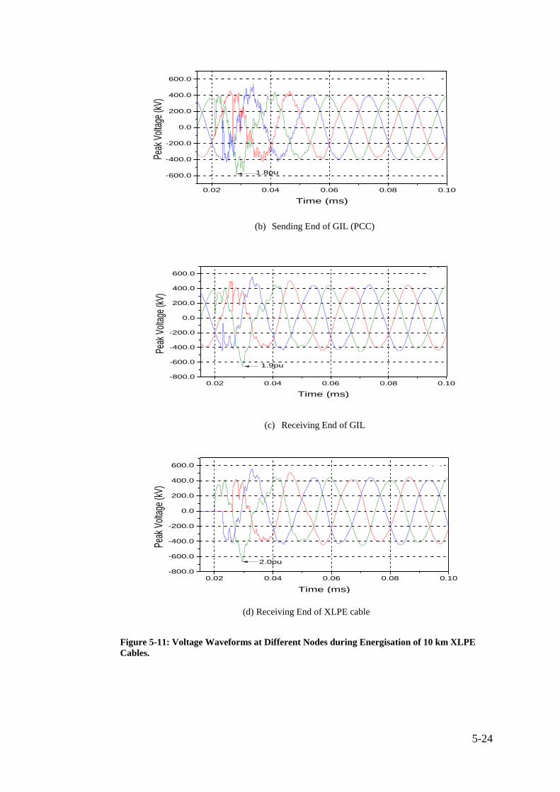
5-24



(d) Receiving End of XLPE cable

Figure 5-11: Voltage Waveforms at Different Nodes during Energisation of 10 km XLPE

Cables.

0.02 0.04 0.06 0.08 0.10

-600.0

-400.0

-200.0

0.0

200.0

400.0

600.0

Peak

Vol

tage

(kV)

Time (ms)

1.8pu

(b)

0.02 0.04 0.06 0.08 0.10-800.0

-600.0

-400.0

-200.0

0.0

200.0

400.0

600.0

Peak

Vol

tage

(kV)

Time (ms)

(c)

1.9pu

0.02 0.04 0.06 0.08 0.10-800.0

-600.0

-400.0

-200.0

0.0

200.0

400.0

600.0

Peak

Vol

tage

(kV)

Time (ms)

(d)

2.0pu

5-25

Figure 5-12: Current through CB5 during Energisation XLPE Cable

5.7.3. Energisation 420/33 kV Offshore Wind Farms

Transformers

Figure 5-13 shows the voltage waveforms during the energisation of the

420/33kV transformers at the offshore wind farm platforms. Closing the three

circuit breakers CB8, CB9 and CB10 connects the already energised XLPE cables

to the 420/33 kV offshore transformers.

The closing time of the circuit breakers was taken from the systematic study. The

corresponding highest overvoltage was found on the randomly switching

operation 101 and at times 20.67ms, 26.67ms and 20.0ms. The current waveform

during energisation of the XLPE cable that flowed through CB5 is shown in

Figure 5-14.

0.02 0.04 0.06 0.08 0.10-8.0

-6.0

-4.0

-2.0

0.0

2.0

4.0

6.0

Peak

Cur

rent

(kA)

Time (ms)

5-26




0.02 0.04 0.06 0.08

-400.0

-300.0

-200.0

-100.0

0.0

100.0

200.0

300.0

400.0

Peak

Vol

tage

(kV)

Time (ms)

(a)

0.00 0.02 0.04 0.06 0.08

-400.0

-300.0

-200.0

-100.0

0.0

100.0

200.0

300.0

400.0

Peak

Vol

tage

(kV)

Time (ms)

(b)

0.00 0.02 0.04 0.06 0.08

-400.0

-200.0

0.0

200.0

400.0

600.0

Peak

Vol

tage

(kV)

Time (ms)

(c)

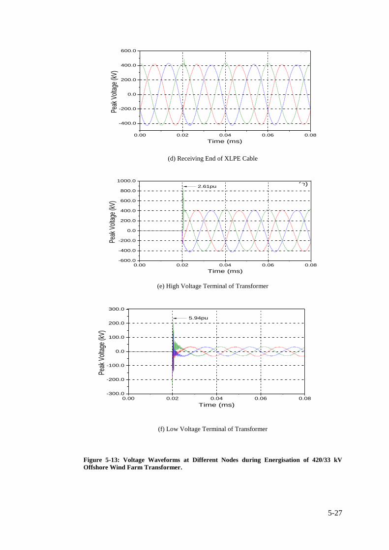
5-27

(d) Receiving End of XLPE Cable

(e) High Voltage Terminal of Transformer

(f) Low Voltage Terminal of Transformer

Figure 5-13: Voltage Waveforms at Different Nodes during Energisation of 420/33 kV

Offshore Wind Farm Transformer.

0.00 0.02 0.04 0.06 0.08

-400.0

-200.0

0.0

200.0

400.0

600.0

Peak

Vol

tage

(kV)

Time (ms)

(d)

0.00 0.02 0.04 0.06 0.08-600.0

-400.0

-200.0

0.0

200.0

400.0

600.0

800.0

1000.0

Peak

Vol

tage

(kV)

Time (ms)

2.61pu(e)

0.00 0.02 0.04 0.06 0.08-300.0

-200.0

-100.0

0.0

100.0

200.0

300.0

Peak

Vol

tage

(kV)

Time (ms)

5.94pu(f)

5-28

Figure 5-14: Current through CB9 during Energisation 420/33 kV Offshore Wind Farm

Transformer

5.7.4. Energisation of 420 kV GIL with trapped charge

Figure 5-15 shows the voltage waveform during the reclosing operation on an

unloaded 300 km GIL for different measurement points.



0.00 0.02 0.04 0.06 0.08 0.10-1.0

-0.5

0.0

0.5

1.0

1.5

2.0

Pea

k C

urre

nt (k

A)

Time (ms)

0.00 0.02 0.04 0.06 0.08 0.10-600.0

-400.0

-200.0

0.0

200.0

400.0

600.0

Peak

Vol

tage

(kV)

Time (ms)

1.48pu (a)

0.00 0.02 0.04 0.06 0.08 0.10-800.0

-600.0

-400.0

-200.0

0.0

200.0

400.0

600.0

800.0

1000.0

Peak

Vol

tage

(kV)

Time (ms)

(b)2.33pu

5-29

(c) Receiving End of GIL.

Figure 5-15: Three-Phase Voltage during Re-closing Operation on Unloaded 300 km GIL

5.8. Effect of GIL Line Length on the Switching Transient

The overvoltage amplitudes due to line energization depend on several factors

including type of circuit-breaker nature, short-circuit power of the bus bar from

which the line is energized and the transmission line length. Therefore, this

section illustrates the effect of different GIL length on the overvoltages generated

during energisation of the GIL under the no load condition. Figure 5-16 shows

respectively the effects of the line length on the maximum overvoltages and 2%

values in 3000 line energizations. Different colours in the figures show different

feeding networks.

0.00 0.02 0.04 0.06 0.08 0.10

-1000.0

-500.0

0.0

500.0

1000.0

1500.0

Peak

Vol

tage

(kV)

Time (ms)

3.6pu(c) 3.96pu

5-30

Figure 5-16: Effect of Different GIL Line Lengths on the Occurrence for Maximum

Overvoltage at the Receiving End for Different Feeding Network Including 2% Value.

As can be seen from Figure 5-16, the overvoltages on GIL lines are more

dependent on the line length. Increase the line length means longer travelling

time for the transient surge to reach the open far end of the line. This increase in

the travelling time will lead to increase the transient surge amplitude. When this

surge gets reflected a higher transient overvoltage will be experienced. From

Figure 5-16 it can be seen that the highest switching overvoltage recorded at the

receiving end of 500 km was 2.80pu which is still within the SIWV limit of

3.1pu.

5.9. Effects of Feeding Network on the Switching Transient

It has been established, from the literature, that the overvoltage amplitudes due to

line energization depend on several factors including type of circuit-breaker

(closing resistor or not), nature and short-circuit power of the bus bar from which

the line is energized. There for in this section the effect of a different feeding

network on the switching transient during energisation different GIL line length

was carried out. Figure 5-17 shows respectively the effects of the feeding

network on the maximum overvoltages and 2% values in 3000 line energizations.

Different colours in the figures show different line lengths.

1.3

1.5

1.7

1.9

2.1

2.3

2.5

2.7

2.9

100 200 300 400 500

Max

imu

m O

verv

olt

age

s (p

u)

Line Length (km)

28.1mH

16.1mH

112mH

1.3

1.5

1.7

1.9

2.1

2.3

2.5

2.7

100 200 300 400 500

2%

Val

ue

Line Length (km)

28.1mH

16.1mH

112mH

5-31

The figures show that the overvoltages in cables have a clear dependence on the

feeding network. The overvoltage level becomes lower for larger source

impedance (weaker feeding network). From Figure 5-17, it is clear that the

overvoltages are more dependent on the line length and the feeding network than

on the line type.

Figure 5-17: Effect of Feeding Network on Maximum Overvoltage for Different GIL Line

Lengths Including 2% Value.

5.10. Summary

The energisation of an unloaded gas insulated transmission line causes high

overvoltage transient and stresses the insulation systems. The level of

overvoltage experienced is governed by many factors, in particular, the problem

underlying sensitivity of CB contacts as well as the characteristics of switching

operation. In this case, attention has been given to the CB pole closing span as

well as the point-on-wave where the contacts initiate their closure.

According to the statistical analysis to the overvoltages distribution data obtained

from simulation approaches for different energisation scenario of 300 km GIL

with offshore transmission network using different pole spans, the switching

transient overvoltage magnitudes are at average level compared to the values

1.5

1.7

1.9

2.1

2.3

2.5

2.7

2.9

0 20 40 60 80 100 120

Max

imu

m O

verv

olt

age

s (p

u)

Source Impedance (mH)

200 km

300 km

400 km

500 km

1.3

1.5

1.7

1.9

2.1

2.3

2.5

2.7

0 20 40 60 80 100 1202

% V

alu

e

Source Impedance (mH)

200 km

300 km

400 km

500 km

5-32

indicated by IEC standard. Overall, for the cases studied using different pole

spans, the range of overvoltages value obtained including the 2% probability of

failure values are within acceptable level and considered to comply with the

standards. Moreover, the risk of insulation failure due to the switching transient

stress applied to the insulation medium was calculated using simplified method

proposed by IEC60071-2. The results have shown that the risk of failure is at low

level which means the risk of insulation is negligible.

The transient overvoltage caused by the trapped charge during re-closing on the

unloaded GIL results in the worst overvoltages at the remote end of the 300 km

GIL. The transient overvoltages was recorded at the receiving end has exceeded

the value specified by IEC by about 27%. The overvoltage is high enough to

cause a failure in the insulation gas. This overvoltage can be avoided by

providing a path for the line to discharge to earth, by connecting a temporary

shunt reactor during energisation of the line.

The overvoltage stress affecting the insulation medium of gas insulation line

increases as the line length increases for different feeding network. Up to 500 km

line length, all the overvoltage magnitudes were within the average level

compared to the values indicated by IEC standard. The network source impedance

also has a strong impact on the overvoltage seen at the receiving end during

energisation of the unloaded GIL. The energisation overvoltages of GIL become

lower for a weaker feeding network

6-1

6 CHAPTER 6: THE PRACTICAL SIDE OF INSTALLING A

“GIL” BASED ON POWER TRANSMISSION PIPLINE

“PTP” TECHNOLOGY

6.1 Introduction

Grid connection for offshore wind farms presents a significant challenge,

especially because of the planned capacities, environmental considerations,

technical constraints, and limited experience regarding offshore power pipeline

projects. Moreover, design power transmission routes complicate the network

development in some subsea areas. This has led to calls for the development of a

new infrastructure solution that can support and advance the development of

offshore wind energy. A new technology based on GIL, which meet the electrical

requirements of connecting large-scale offshore wind farms, has recently received

attention. This technology is known as ‘power transmission pipelines’ or (PTP)

[118].

The construction and operation of a PTP system and other tubular structures

offshore presents great challenges and unique design needs, which sometimes

require the development of new technologies, such as new underwater surveying

technologies, a variety of methods and associated vessels for installing pipelines

in increasingly deeper waters, new corrosion protection methods and insulation

materials, submarine welding and monitoring methods and facilities, seafloor

trench digging methods, remotely controlled vehicles, and equipment for deep

water operations [119], [120].

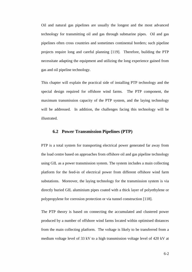
6-2

Oil and natural gas pipelines are usually the longest and the most advanced

technology for transmitting oil and gas through submarine pipes. Oil and gas

pipelines often cross countries and sometimes continental borders; such pipeline

projects require long and careful planning [119]. Therefore, building the PTP

necessitate adapting the equipment and utilizing the long experience gained from

gas and oil pipeline technology.

This chapter will explain the practical side of installing PTP technology and the

special design required for offshore wind farms. The PTP component, the

maximum transmission capacity of the PTP system, and the laying technology

will be addressed. In addition, the challenges facing this technology will be

illustrated.

6.2 Power Transmission Pipelines (PTP)

PTP is a total system for transporting electrical power generated far away from

the load centre based on approaches from offshore oil and gas pipeline technology

using GIL as a power transmission system. The system includes a main collecting

platform for the feed-in of electrical power from different offshore wind farm

substations. Moreover, the laying technology for the transmission system is via

directly buried GIL aluminium pipes coated with a thick layer of polyethylene or

polypropylene for corrosion protection or via tunnel construction [118].

The PTP theory is based on connecting the accumulated and clustered power

produced by a number of offshore wind farms located within optimised distances

from the main collecting platform. The voltage is likely to be transferred from a

medium voltage level of 33 kV to a high transmission voltage level of 420 kV at

6-3

each collecting wind farm platform in order to reduce the losses to the lower level

during the transmission of electrical power to the main collecting platform for

feed-in [121].

At the main collecting platform, the bundled power is connected to the

transmission system, that is, the GIL, to transmit the power to the onshore

connecting point. The GIL form the core for the PTP technology as a

transmission system lay in a tunnel under the seawater or coated with a thick

passive corrosion protection layer for carrying power to the shore. Figure 6-1

shows a visualisation of the PTP offshore transmission solution.

Figure 6-1: Visualisation of PTP Offshore Transmission Solution [122]

6.3 PTP Offshore Design Consideration

The construction of an offshore PTP requires the involvement of several

engineering disciplines. A survey of the installation site has to be commissioned

before the route of the pipelines is selected. The water depth and sea floor tenacity

6-4

for the pipelines route define the load that can be applied to the sea floor as well

as the installation method chosen for the project.

Furthermore, several impediments that may affect the final route selection need to

be taken in consideration, such as political issues in the case of crossing other

countries territorial waters; geological hazards, such as earthquakes and volcanos;

physical factors along the prospective route; and other users of the seabed in the

selected area. This task starts with a survey of geological maps, fishing charts,

and aerial and satellite photography, as well as information from navigation

authorities [119].

6.3.1 Physical Factors

The physical factors that need to be considered at the beginning are the state of

the seabed, that is, whether it is relatively flat or rough with high hills. If the sea

floor has high hills, the PTP will include free spans. When the PTP is placed on

high points, there will be unsupported sections between these points. If the

unsupported sections are too long, the bending stress applied to them due to their

weight may cause the PTP to bend. Therefore, corrective measures for

unsupported PTP spans with post installation support, such as berm or sand

infilling below the PTP, are very important. The solidity of the sea floor is

another important factor; if the soil is not strong enough to withstand the weight

of the PTP, the PTP may sink into it [120].

6.3.2 Other Users of the Seabed

Western Europe, including the North Sea, falls into the International Council for

exploration and monitoring of human activities in the seas [123]. Therefore,

6-5

proper planning of a PTP has to take in a wide range of human activities that may

affect the seabed along the proposed route or that are likely to do so in the future,

such as other pipelines, fishing vessels, ships anchors, and military activities. The

offshore PTP pipelines are major structures with costs that run into the hundreds

of millions of pounds; thus, they need and deserve to be designed carefully with

all the care and attention that modern engineering tools can provide [120].

6.4 PTP System Design

6.4.1 Model of an AC Offshore Solutions

Each feeder consists of a number of turbines; these will be connected to an

offshore collector platform, located in an appropriate place to minimise the feeder

cable lengths required. At the offshore collector platform, the generated power

will be transformed from a medium voltage level to a higher voltage level to

transmit the generated power to the PTP main collection platform with minimum

power loss using AC cables as the connection medium. The cross section and the

number of cables will be determined based on the amount of power generated and

the transmission voltage level. The voltage level will be determined by detailed

studies, but it is likely to be 420 kV or 550 kV [121].

The number of collector substations for the project will be determined based on

detailed studies. An immersed tunnel is one of the laying technology options for

the PTP system design, not only from the economic point of view but also for

safety and reliability reasons; the tunnel should have at least two three-phase

transmission circuits. The special design of the tunnels can give a space for four

three-phase systems with a total power of 4*3000 MW. Figure 6-2 shows a

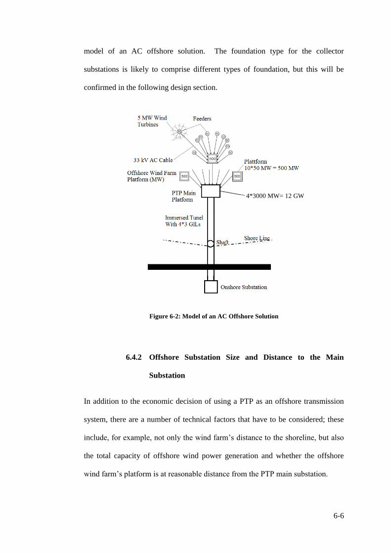
6-6

model of an AC offshore solution. The foundation type for the collector

substations is likely to comprise different types of foundation, but this will be

confirmed in the following design section.

Figure 6-2: Model of an AC Offshore Solution

6.4.2 Offshore Substation Size and Distance to the Main

Substation

In addition to the economic decision of using a PTP as an offshore transmission

system, there are a number of technical factors that have to be considered; these

include, for example, not only the wind farm’s distance to the shoreline, but also

the total capacity of offshore wind power generation and whether the offshore

wind farm’s platform is at reasonable distance from the PTP main substation.

4*3000 MW= 12 GW

6-7

The maximum power transmission capacity is limited by the cross section of the

AC cables and the amount of reactive power generated by the cable shunt

capacitance where the reactive power is proportional to the square voltage level.

Based on the ABB and Prysmian models [124], [125], the 2500 mm2 XLPE cable

for offshore application can transmit up to 800 MVA at 420 kV per three-phase

system.

The technological advancement of the PTP system, which utilizes GIL as a main

connection medium, reconfirmed that, based on the conductor and enclosure cross

sections, a single three-phase circuit of GIL can transmit power up to 4000 MVA

at 420 kV [78]. The largest distance from the individual wind farms to the PTP

main substation is generally less than 20 km as stated in the report [121]. Beyond

a certain distance from the main PTP substation, AC cables lose their

attractiveness as an option and are no longer economically viable for the

connection of the wind farms to the PTP main substation.

6.5 PTP Laying Technology

Constructing a subsea tunnel for such line lengths is not an easy task. A subsea

tunnel represents the biggest percentage of the cost of the overall system cost, but

in some cases, it is still central to the PTP system for a variety of reasons. Unlike

the oil and gas pipelines, which are made from steel pipes, the PTP pipe is made

from an aluminium alloy, which is weaker than steel and has a low corrosion

resistivity. Strength and corrosion resistivity are required characteristics for

offshore pipelines to resist collapse due to external pressure and to extend the

pipeline’s life.

6-8

The wall thickness of the gas and oil pipelines ranges from 11.4 mm to 38 mm

depending on the type of goods and the water depth [119], whereas the wall

thickness of the GIL ranges from 6.4 mm for 420 kV to 9.5 mm for 1200 kV[78].

Therefore, there are three options to meet these requirements: installing GIL pipes

in a subsea tunnel, which is the most expensive option; coating GIL pipes with a

thick layer of polyethylene; or installing the GIL pipes in another steel pipe,

which is called pipe in pipe laying technology.

6.5.1 GIL Tunnel Laying Option

6.5.1.1 Tunnel Constructed with a Tunnel Boring Machine

The exact method of tunnel construction, that is, with a tunnel-boring machine

(TBM) or a drilled tunnel, depends on the geological and hydrogeological

conditions along the selected route. The basic concept of building a tunnel is that

the ground is dismantled gradually under the protection of a shield. The tunnel

tubes are lined with waterproof concrete shell elements. The required equipment

and material are brought into the tunnel through the tunnel portal using a transport

system. Excavated material is taken out using the same route. Intermediate

constructions, such as shafts, are not necessary using this construction technique.

The main purpose of a drilled tunnel is to bridge a certain distance from land into

the sea, which will then be connected to a subsea immersed tunnel; a shaft is

required at this point [126].

Finishing the tunnel is the most difficult stage of construction of a PTP system.

Subsequently, the GIL pipes are fitted inside the tunnel. The tunnel features

include energy supply, ventilation, monitoring and communications systems as

well as a transport system. The transport system is necessary to overcome the

6-9

long tunnel distances during the construction period and later for servicing

purposes. Tunnels are constructed usually with four three-phase systems both for

economic reasons and for operational and personnel safety reasons. Two tunnel

construction methods are available: a closed construction tunnel using a TBM,

such as those used worldwide for the construction of traffic tunnels, and the

immersed tunnel method, which forms a part of current offshore building

techniques [126].

6.5.1.2 Immersed Tunnel

The immersed tunnel is a kind of underwater tunnel composed of concrete

segments, constructed in another place, and floated to the tunnel site to be sunk

into place after they have been connected together. Immersed tunnels are usually

used in combination with other forms of tunnel at both ends, such as a drilled

tunnel or bored tunnel, as this is usually necessary to continue the tunnel from

near the water’s edge to the entrance at the land surface. Figure 6-3 shows a cross

section of prefabricated immersed tunnel segments [126].

The tunnel is fabricated in separate segments, with each segment prefabricated in

a manageable length. The ends of each segment are blocked with bulkheads so

they can be floated. At the same time, the corresponding parts of the tunnel path

are prepared, with a submarine trench in the selected route being dredged and

graded to fine tolerances to support the elements. The next stage is to place the

segments into place; each is towed to the final location and in most cases,

assistance is required to keep the segments buoyant. Once the segments have

been placed in the required position, additional weight is used to sink the

elements into the final location; this is the most critical stage as it is essential to

6-10

ensure that each piece is aligned correctly. Once this stage is finished, the joint

between the new element and the tunnel is dewatered and then made watertight;

this process is continued sequentially along the tunnel [126].

The trench is then backfilled and any necessary protection, such as rock armour,

added over the top. The ground beside each end tunnel element will often be

reinforced, to permit a TBM to drill the final links to the portals on land. Once

these stages have been finished, the tunnel is complete and the internal fit out can

be carried out [126].

The segments of the tube may be constructed using one of two methods. The first

method is to construct steel or cast iron tubes, which are then lined with concrete.

This allows the use of conventional ship building techniques, with the segments

being launched after assembly in dry docks. The second method, which is a

reinforced concrete box tube construction, has been the standard; the sections are

cast in a basin, which then flooded to allow their removal [126].

Figure 6-3: Prefabricated Immersed Tunnel Segments [122]

6-11

6.5.1.3 Fitting GIL inside the Tunnel

GIL is laid after the completion of the tunnel. Preassembled GIL pipes are

delivered to the landing shaft and lowered into the shaft using a crane. In the

welding tent, individual elements are completely assembled, welded together, and

then pulled into the tunnel. The GIL is kept on rollers or mounts equipped with

sliding contact bearings, which allows for thermal expansion of the coat tube. The

compensator units, built in at regular intervals, permit the respective thermal

expansion in the conductor tubes.

6.5.2 GIL Coated Pipes

Coating the GIL pipes with a thick layer of polyethylene or polypropylene is the

cheapest and most trouble free installing method. Adding a thick layer of

polyethylene or polypropylene can give the pipe the physical strength required to

withstand the external pressure and provide corrosion protection as well [127].

The global pipeline manufacturers have developed a high quality polyethylene

and polypropylene coating for aluminium and steel pipes for the transmission of

gas, oil, water, and other fluids, making the pipes highly resistant to corrosion

from moisture, chemicals, and other harmful substances. The thickness of the

coated layer depends on the external pressure that will be applied to the pipe,

which is strongly related to the water depth. Figure 6-4 shows the coating process

of the aluminium pipe [127].

6-12

Figure 6-4: Coating Process of Aluminium Pipe [127]

6.5.3 Pipe in Pipe Layout Technology

Due to the high cost of the immersed tunnel and the special protection

requirement of the aluminium GIL in a seawater environment, the pipe in pipe

technology and the concrete coated pipe are recently being considered. Pipe in

pipe technology can offer a cheaper solution and less installation effort than an

immersed tunnel. In this case, the protective steel casing pipe and the GIL are

laid together as a PTP system. Figure 6-5 shows the pipe in pipe

technology[128].

As with offshore pipelines from the oil and gas industry, laying takes place on

offshore pipe laying vessels. Here, the entire assembly of the GIL and casing

pipes is carried out aboard the ship. During the laying process, the tough

requirements of the PTP regarding external conditions during construction are of

paramount importance. In addition to procedures for laying, welding, and

connecting along the various pipes, material properties must be taken into account

6-13

during construction. As the laying, operational, and repair technology of this

extremely complex pipe in pipe system will not be available for the foreseeable

future, this concept is currently considered a future option[128].

Figure 6-5: Pipe in Pipe Layout Technology [128]

6.6 Offshore Wind Farm Substations and Platforms

The traditional voltage level for connecting offshore wind turbines to the

medium-voltage wind farm collection system is 33 kV. However, due to the

maximum transmission capacity limit, it is not possible to transmit generated

power to the onshore grid at this voltage level. Hence, for many of the projects,

offshore substations are required to accumulate the power from the internal wind

farm cable arrays and step up the voltage to an appropriate level for transmission

over long distances.

The amount of power that can be accumulated at the PTP main offshore

substation and the number of offshore wind farm substations required for the

project will be decided by the total power carrying capacity of the onward

transmission medium. The power carrying capacity of the array cabling and the

6-14

number of wind turbines will determine the size of the offshore wind farm

substations. The distance from the platform to the furthest wind turbine in the

array must also be taken into consideration, as using excessive lengths of 33 kV

cable to connect an array can lead to excessive power losses.

An offshore wind farm platform is required to house the substations that gather

the wind turbine connection cables. A step up transformer and switchgear are the

main components. A bus bar and additional control and measurement equipment

are required as well. Export cables then connect the offshore wind farm

platforms, generally by HVAC cables, to the PTP main substation for feed-in

power to the PTP transmission system to shore.

The PTP main substation is shown in Figure 6-6. It is designed to house the

substation that gathers the connection cables of the offshore substation platforms.

Platform topsides are supported on jackets made from steel pipes each having

three to eight legs piled into the seabed. Monopiles can be used for smaller

platforms.

In addition to housing transformers, cooling radiators, fans, switchgears, and the

associated control panels, the platform will typically include emergency

accommodation and life-saving equipment, a crane for maintenance lifts, a winch

to hoist the subsea cables, a backup diesel generator, fuel, a helipad,

communication systems, and the means to support the J-tubes that contain the

subsea GIL [128].

6-15

Figure 6-6: The PTP Main Substation [128]

6.7 Shafts

Three types of shafts are required during the construction of a PTP system:

working shaft, reception shaft and intermediate shaft. All shafts should be of an

appropriate size to permit safe temporary access for construction work and

operational access to the completed tunnel; for the insertion and removal of

electrical and services equipment, such as preassembled GIL segments; and for

the safe installation and removal of the TBM and its equipment. The working

shaft and reception shaft can be removed after finishing the construction process.

Figure 6-7 shows an intermediate shaft for a PTP system [128].

6-16

Figure 6-7: Intermediate Shaft for PTP System [128].

6.8 PTP System Construction Challenges

As explained previously, the PTP project is a field with great challenges and

unique design needs. The PTP developer needs to concentrate on the techno-

economic assessment of the offshore projects, which are strongly affected by

policy trends, regulatory issues, and industry developments [129].

Identifying a concrete path for the PTP project after the spatial analysis for the

maritime area will ensure the technical and political feasibility of the project.

This will force the developer to accept some regulatory, industry or policy issues.

Once the developer has identified an optimal offshore grid design, the next

question raised is whether the design can be done within a reasonable time frame.

More challenges are discussed below [129].

6.8.1 Operation and Maintenance of an Offshore Grid

Offshore grid faults have to be cleared as soon as possible with quick and large

primary control actions, especially in the case of high wind penetration. The

6-17

question is whether these primary control actions already exist at all sites. If not,

their construction or market integration is a necessary condition for maintenance

of an offshore grid. The offshore grid outage can take longer to repair than is the

case for an onshore grid, due to difficulties accessing the offshore equipment [6],

[129].

In general, the maintenance costs for the offshore grid are much higher than for

the onshore grid, mainly due to offshore weather variations during the seasons

and a small number of offshore cable production. At the aggregate level (PTP),

based on the long experience gained from onshore insulation, the GIL does not

require much maintenance. Therefore, maintenance issues are a minor issue for

the offshore PTP system itself.

In the case of a fault leading to a failure in the PTP system, a very good

monitoring system is required to identify the exact place of the failure. Due to the

special design of the GIL, there are disconnecting units placed every 1200 m to

1500 m to separate the insulation gas and to connect high voltage test equipment;

this makes it possible to repair the failed section without releasing all the

insulation gas.

6.8.2 Operational Responsibilities and Offshore Grid Codes

As mentioned previously, most of the developed projects occur in the North Sea.

Therefore, some of the planned projects will be shared between countries. The

clear division of operational responsibilities for an international offshore grid is

more complicated than for between national transmission operators. In addition,

the agreement of which offshore grid codes should be used represents a challenge.

The development of European network codes as initiated by the European

6-18

Commission, which is expected to be made public very soon, is the first step

towards overcoming this challenge. Uniform grid connection requirements need

to be determined for connecting wind plants to the transnational offshore grid

[6],[7],[129].

6.8.3 Financing the Large Investments

Establishing such offshore grids will be expensive due to the large amount of high

cost equipment and the high cost of installing this equipment in an offshore

environment. The overall benefits of an international offshore grid from the

system perspective cannot directly be returned to the investor. Therefore, an

indication of long-term commitment and reliability in national offshore policies is

needed to attract investors. Otherwise, investments in onshore and offshore grid

infrastructure will not be made in sufficient magnitude. In addition, it may be the

case that publicly funded securities are needed to give a breakthrough for

pioneering offshore investments. At the aggregate level, raising enough funds for

an offshore grid is viewed by the offshore grid consortium as a major challenge

[6], [7], [129].

6.9 Summary

The PTP system is an AC transmission system for high and extra high voltage

based on GIL. Compared to other transmission technology, a PTP system has

high transmission capacity; a low power loss, which means high efficiency; and a

high overload capacity. Moreover, it allows the transfer of bulk power over long

distances.

6-19

The idea of a PTP system is based on clustering wind power projects in one main

substation. Sharing the transmission system offers the most advantages. When a

high number of wind farm capacities are connected in a small area and when the

clusters’ capacities are about the standard size of the PTP transmission system,

sharing one transmission system can reduce the amount of planning, installation,

and maintenance and can even be more economical than individual connections.

In addition, apart from the economic comparison with other transmission

technologies, a PTP system can help to mitigate the environmental and social

impact of laying multiple cables through sensitive coastal areas and allow for

more efficient logistics during installation. These benefits need to be balanced

with the risk of bounded investments.

7-1

7 CHAPTER 7: ECONOMIC COMPARISON OF

ESTIMATION COST FOR HVAC-PTP AND HVDC-VSC

OFFSHORE TRANSMISSION SYSTEMS

7.1. Introduction

The decision to use HVAC or HVDC transmission technology involves an

economic analysis of the proposed project where the costs of the transmission

line, stations, and power losses have to be considered. As mentioned in previous

chapters, the rapid growth in the development of offshore wind farms requires a

transmission system with high transmission capacity and low power losses [6].

Moreover, the capability of transmitting power over long distances is an

important feature. Therefore, due to their capability of transmitting high power

over long distances, an economic comparison has been made between two

possible offshore transmission technologies: HVAC-PTP and HVDC-VSC

systems. The most difficult part of this study was finding the most recent data

concerning the cost of the various components of the transmission technologies

that are under investigation. This is because the related industry treats this

information and data as confidential, or they just give estimated data.

In this chapter, the total build costs of a new transmission system for both

transmission technologies have been estimated; these are subdivided into the

fixed build cost and the variable build cost. The variable operation cost has been

estimated as well and has been divided into maintenance cost and power losses

cost during the lifetime of the equipment. The overall lifetime cost of both

7-2

transmission technologies has been estimated as lifetime cost per km. The power

transmission cost (PCT) has been calculated as lifetime cost per km for each

MVA/MW being delivered to the receiving end of the proposed transmission line

length.

7.2. Proposed Transmission Systems

Two basic factors affect the total cost of any electrical transmission system: the

amount of power they are expected to transfer and the length of the transmission

line. In this study, two different transmission capacities have been considered.

The HVAC-PTP low transmission capacity consists of two AC circuits, each of

2000 MVA at 420 kV, whereas the HVAC-PTP high transmission capacity

consists of two AC circuits, each of 3180 MVA at 420 kV.

The HVDC-VSC low transmission capacity consists of two DC bi-poles, each of

1500 MW at ± 320 kV while the high transmission capacity consists of four DC

bi-poles, each of 1500 MW at ± 320 kV. Two basic route lengths have been

chosen to carry out this comparison study. The first is a 75 km line length, as this

distance is the maximum economic distance for utilizing XLPE cables as a

transmission system, and the second is a 300 km line length, which can fulfil the

transmission distances required for an offshore development scenario in the North

Sea with the transmission equipment having a lifetime of 25 years.

It should be noted that two layout options for the PTP technology have been

considered, the first option is directly buried aluminium pipes coated with a thick

layer of PE or PP, and the second option is aluminium pipes laid in a subsea

7-3

tunnel. However, the only layout option for HVDC technology under

consideration is directly buried cables under the seabed.

These choices have been made based on a consideration of future offshore wind

farm requirements with a close evaluation of planned projects in the Dogger Bank

Teesside project, Round 3 in the UK, and German planned projects in the North

Sea [130], [121].

The main components of the total cost of the HVAC-PTP transmission

technology are: the main collection substation, the GIL equipment including the

insulation gas, and the layout technology option, that is, whether it is coated with

a PE insulation layer or installed inside a subsea-constructed tunnel. The main

components of the total cost of HVDC-VSC transmission technology are the

converter stations both offshore and onshore, the DC cables, onshore land use,

and the offshore substations.

The implementation of such large projects is extremely complicated and involves

many factors and variables that affect their total economic cost; however, many of

these are not recognized by the public. Such costs include the settlement cost of

the seabed the transmission connection runs through; the onshore land cost for the

onshore substation; the world metal price, which fluctuates daily, and the cost of

labour.

The blue boxes in Figure 7-1 show the boundaries of each transmission system

considered in this calculation. The offshore wind farm platform and its electrical

equipment, including the XLPE cables connecting the wind farm collection points

to the main collection substations, are considered as forming part of the wind-

farm generation side rather than the transmission system side [131].

7-4

Figure 7-1: Transmission System Boundaries (A) HVAC-PTP System, (B) HVDC-VSC

System

7.3. Economic Comparison

7.3.1. Introduction to the Lifetime Cost Method

The following steps indicate the method used to calculate the lifetime cost [132]:

The total build cost for each new transmission technology has been

divided into the fixed build cost and the variable build cost. The fixed

build cost is not dependant on the length of the new transmission system

being constructed, such as costs for project planning and management and

equipment for the termination of the transmission line at both ends, that is,

offshore and onshore. The variable build cost varies depending on the

transmission system length, such as costs for studying the route and the

transmission line layout option requirements.

7-5

Variable operation costs also include costs that depend on the length, such

as the cost for the transmission line and whether it is conventional cable or

aluminium pipes, including the insulation gas. Moreover, the maintenance

of the equipment during its lifetime and the power losses costs are also

included. These costs increase over the lifetime of the equipment. The

sum of the fixed build cost, the variable build cost, and the variable

operation cost combine to make the total lifetime cost.

By dividing the lifetime cost by the length of the transmission system, the

value of the lifetime cost per km can be calculated.

By dividing the lifetime cost per km by the total transmission capacity, the

power transfer cost (PTC) for each MVA/MW delivered to the receiving

end can be calculated, which will compensate for the difference in the

transmission capacities between the proposed transmission systems.

7.3.2. Initial Investment Cost

The transmission systems component costs data were taken from the most recent

electrical transmission costing reports. In 2012, European Network of

Transmission System Operators for Electricity (ENTSOE) prepared a report for

the EU about different offshore transmission technology options and their costs

[133]. Moreover, on 31 January 2012, the Institution of Engineering and

Technology and Parsons Brinckerhoff published a report about the costs of a new

electricity transmission infrastructure [132].

The price given in [132] was based on the British market and the British currency;

this study has been shown by the UK national grid on February 2012 to be a very

valuable costing data source [134]. For other price sources, exchange rates of

7-6

GBP£/EUR€ = 0.88 and EUR€/US$ = 1.4 [132] have been used to convert the

price to pounds sterling.

The previous sources considered in this study are considered the most recent and

reliable sources since their authors have listed as their price sources most of the

industrial companies that have a relationship with this kind of projects, which has

provided them with the most accurate data. However, none of them have costs

for an offshore transmission system 300 km from the shore; therefore,

adjustments have been made in order to match the specific characteristics of the

proposed transmission systems.

7.3.3. HVAC-PTP Investment Cost

7.3.3.1. Total Fixed Build Cost

The overall fixed build cost comprises the costs for project launching and

management studies; the PTP main substation; and the equipment needed at both

ends, such as GIL termination equipment compatible with air-insulated

switchgear. It also includes the cost of the transmission line route selection.

According to [132], the fixed build cost value for 75 km of directly buried GIL

aluminium pipes with 2*2000 MVA low transmission capacity is £7.4 M.

However, the fixed build cost of 2*3190 MVA high transmission capacity is

similar to the fixed build cost of low transmission capacity, due to the high

transmission capability of GIL, which can transmit up to double the low

transmission capacity with no additional equipment [19].

Moreover, the total fixed build cost value for 75 km GIL aluminium pipes laid

inside a subsea tunnel and having low transmission capacity is £278.2 M [132].

7-7

The fixed build cost of high transmission capacity is also similar to the fixed build

cost for low transmission capacity for the same reason. It can be noted that the

big difference in the fixed build cost for both layout options is due to the high cost

of the subsea tunnel construction.

The fixed build cost value for 300 km line length and directly buried GIL

aluminium pipes is £7.4 M for both low and high transmission capacities.

However, the fixed build cost value for 300 km GIL installed inside a subsea

tunnel for both low and high transmission capacities increases to £1090.6 M.

This cost was calculated based on assumption taken from [132]. The fixed build

cost value for 300 km was calculated by multiplying the cost of 75 km cost for the

components depend on the transmission line length by four times [132]. The

components that make up the total fixed build cost for both layout options and

different transmission capacities for both 75 km and 300 km are shown in Table

7-1.

Table 7-1: Estimated Total Fixed Build Cost for both Layout Options and Different

Transmission Capacities for 75 km and 300 km HVAC-PTP Transmission Technology [132].

Fixed Build

Cost Component

Directly

Buried GIL 2*2000 MVA

75 & 300 km

GIL In

Tunnel 2*2000 MVA

75 km

GIL In

Tunnel 2*2000 MVA

300 km

Directly

Buried GIL 2*3180 MVA

75 & 300 km

GIL In

Tunnel 2*3180 MVA

75 km

GIL In

Tunnel 2*3180MVA

300 km

GIL

Termination

(AIS) and Testing

£2.3 M

[132]

£2.3 M

[132]

£2.3 M

£2.3 M

[132]

£2.3 M

£2.3 M

GIL Terminal

Compound

£5.1 M

[132]

£5.1 M

[132]

£5.1 M

£5.1 M

[132]

£5.1 M

£5.1 M

Tunnel + Shafts

Design and Equipment

-

£149.6 M [132]

£598.4 M

-

£149.6 M

£598.4 M

Tunnel Boring

Machine Cost

-

£23.6 M

[132]

£94.4 M

-

£23.6 M

£94.4 M

Tunnel PM

-

£97.6 M [132]

£390.4 M

-

£97.6 M

£390.4 M

Total Fixed

Build Costs

£7.4 M

[132]

£278.2 M

[132]

£1090 M

£7.4 M

[132]

£278.2 M

£1090 M

7-8

7.3.3.2. Total Variable Build Cost

The variable build cost makes up the biggest part of the total lifetime cost. The

variable build cost of the PTP covers the cost of those items that principally vary

by transmission line length. The material and the insulation gas cost for the GIL

aluminium pipes required for the proposed line length is included in the variable

build cost. The costs associated with construction of the tunnel and shafts are also

included.

The volume of the aluminium material required for the GIL pipes is defined by

the diameter of the pipe and the wall thickness of the pipe. The diameter of the

pipe is defined by the rated voltage for the enclosure and the conductor pipe.

Depending on the power to be transmitted per circuit and the voltage level the

volume of aluminium required can be calculated.

For 420 kV GIL, 1 km of single phase GIL aluminium pipe requires 47.310

tonnes of aluminium material [78]. To make a three-phase circuit requires 141.93

tonnes per km. For example, 300 km of GIL requires 42579 tonnes of aluminium

material. The price of aluminium on the international metal markets in January

2012 was £1867 per tonne [132]. Based on this calculation, the total aluminium

material required for 300 km GIL costs £79.495 M. It should be noted that this

cost does not include the sampling of GIL pipes and fitting the conductor inside

the enclosure with all the equipment required and the outer PE insulation coated

layer.

The volume of the insulation gas required for a 1 km single-phase GIL is 5.72

tonnes, which makes 17.16 tonnes per three-phase system [78]. In addition, 5148

tonnes of insulation gas are required for 300 km. CF3I is the insulating gas

7-9

considered for this calculation. However, as noted in the literature review, CF3I is

a new artificial gas, and its production still does not meet the industrial

requirement [135].

Recently, at least two manufacturers have invested in producing commercial

quantities of CF3I to create sufficient capacity to fulfil all foreseeable

requirements. Active competition is already occurring, and the price of CF3I has

been reduced from over £630 per kg to around £62.86 per kg at present [136].

For this calculation, the price of £62.86 per kg has been used, which makes a total

cost of £323.6 M.

It should be notes that, the recovery of aluminium pipe material and the disposal

of insulation gas after 25 years lifetime was taken in consecration in [132]. The

increase of the aluminium material cost on the international metal markets has

reduced the variable build cost by 10% after the accounting of the cost of

extracting the aluminium pipes from the sea bed and the disposal of the insulation

gas.

According to [132], which has considered all previous factors, the total variable

build cost for 75 km of directly buried GIL aluminium pipes for low transmission

capacity is £937.4 M. The variable build cost of high transmission capacity is

also similar to the variable build cost of low transmission capacity because no

additional equipment is required.

The total variable build cost value for 75 km of GIL aluminium pipes inside a

subsea tunnel for low transmission capacity is £1606 M, which is similar to the

variable build cost of high transmission capacity [132]. The components making

7-10

up the total variable build cost for a 75 km line length and both layout options are

shown in Table 7-2.

The total variable build cost for 300 km with both layout options was calculated

based on the same assumption taken from [132]. The fixed build cost value for

300 km was calculated by multiplying the cost of 75 km for the components

depend on the transmission line length by four times [132]. The total variable

build cost for 300 km directly buried GIL with low transmission capacity is £3750

M, which is equal to the cost of high transmission capacity. The total variable

build cost for 300 km of GIL installed inside a subsea tunnel is equal to £6424 M.

This cost is similar to the variable build cost of high transmission capacity. The

components making up the total variable build cost for a 300 km line length and

both layout options are shown in Table 7-2.

Table 7-2: Estimated Variable Build Cost of Different Layout and Different Transmission

Capacities Options for 75 km and 300 km HVAC-PTP Transmission System.

Variable Build Cost Component

Directly Buried GIL 2*2000 MVA

2*3180 MV

75 km

GIL In Tunnel 2*2000 MVA

2*3180 MV

75 km


2*3180 MV

300 km


2*3180 MV

300 km

Equipment Costs

(GIL Aluminium Tubes + Gas

insulation)

£561.2 M [132]

£561.2 M [132]

£2244.8 M

£2244.8 M

Civil Costs Including

EP Coating Layer or

Special Tunnel Construction

£131.3 M

[132]

£211.2 M

[132]

£525.2 M

£844.8 M

Project Launching +

mgmt.

£140 M

[132]

£140 M

[132]

£560 M

£560 M

Build Contingency (GIL)

£105 M [132]

£489.4 M [132]

£420 M

£1957.6 M

Tunnel Boring Machine Costs

-

£147.5 M [132]

-

£590 M

Tunnel PM

-

£56.7 M

[132]

-

£226.8 M

Total Variable Build

Costs

£937.5 M

[132]

£1606 M

[132]

£3750 M

£6424 M

7-11

7.3.3.3. Total Operation Cost

The variable operation cost is a combination of the operating and maintenance

costs. The cost related to power losses at the power station and the transmission

system as well the cost for reactive power compensation. In general, the real

power losses in the GIL are relatively low, as was shown in Chapter 4,

comprising less than 2% of the total power losses for a 300 km GIL line length.

Wind farms have a variable output and they will not operate at their full

nameplate capacity all the time. Therefore, the GIL will not operate at 100% load

condition. As the load condition decreases the voltage drop at the load bus

increases which require reactive power compensation to be connected to the load

bus to maintain the bus voltage within acceptable limit.

The normal way of controlling the voltage drop is to install reactive power

compensation in the form of shunt reactors or shunt capacitors. the capacitor

affect in the GIL line is high than the inductive affect, but due to the large

inductive load connected to the bus load, the GIL will require capacitive reactive

power compensation to be connected at the load bus.

These compensation devises are, however, large and expensive. According to

[133] the cost of supplying and installing a 200 Mvar capacitor has been

estimated to be £5.786 M. Thus the cost of reactive compensation has been

estimated to be £28.9 per Mvar.

According to the reviewed literature, the gas-insulated technology does not

require much maintenance during their lifetime. Therefore, the variable operation

cost for 75 km of directly buried GIL is £37.3 M for low transmission capacity

7-12

whereas the variable operation cost for high transmission capacity is £48.2 M

[132].

The total variable operation cost for 75 km of GIL inside a subsea tunnel is

£54.85 M for low transmission capacity whereas the variable operation cost for

high transmission capacity is £70.9 M [132]. The components making up the total

variable operation cost for both layout options are shown Table 7-3.

Table 7-3: Estimated Variable Operation Cost of Different Transmission Capacities and

Different Transmission Layout Options for 75 km PTP Transmission System [132].

Variable Operation Cost

component

Directly Buried

GIL 2*2000 MVA 75 km

GIL In Tunnel

2*2000 MVA 75 km

Directly Buried

GIL 2*3180 MVA 75 km

GIL In Tunnel

2*3180 MVA 75 km

Cost of Power Losses (Station) £10.4 M £10.4 M £15.3 M £15.3 M

Cost of Energy Losses (Fuel) £18.2 M £18.2 M £18.2 M £18.2 M

Operation and Maintenance £8.7 M £19.6 M £21.35 M £37.4 M

Total Variable Operation Cost £37.3 M £48.2 M £54.85 M £70.9 M

The variable operation cost for 300 km of directly buried GIL is £149.2 M for low

transmission capacity whereas the variable operation cost for high transmission

capacity is £219.4 M.

The total variable operation cost for 300 km of GIL aluminium pipes inside a

tunnel is £192.8 M for low transmission capacity whereas the variable operation

cost for high transmission capacity is £283.6 M. The components making up the

total variable operation cost for both layout options are shown in Table 7-4.

7-13

Table 7-4: Estimated Variable Operation Cost of Different Transmission Capacities and

Different Transmission Layout Options for 300 km PTP Transmission System

Cost component Directly Buried GIL 2*2000 MVA

300 km


300 km


300 km


300 km

Cost of Power Losses (Station) £41.6 M £41.6 M £61.2 M £61.2 M

Cost of Energy Losses (Fuel) £72.8 M £72.8 M £72.8 M £72.8 M

Operation and Maintenance £34.8 M £78.4 M £85.4 M £149.6 M

Total Variable Operation Cost £149.2 M £192.8 M £219.4 M £283.6 M

7.3.3.4. HVAC-PTP Total Lifetime Cost

The lifetime cost for both different HVAC-PTP layout technologies and different

transmission lengths are shown in Table 7-5.

Table 7-5: Calculated Lifetime Cost with both Different Layout Technologies and Different

Transmission Capacities for 75 and 300 km Line Length

Cost component Directly Buried GIL 2*2000 MVA




75 km Line length

Total lifetime cost £982.2 M £1932.4 M £999.75 M £1955M

Lifetime cost per km £13.1 M £25.8 M £13.33 M £26.1 M

Power Transfer Cost

£/MVA-km

3274

£/MVA-km

6441.3

£/MVA-km

2096

£/MVA-km

4104

£/MVA-km

300 km Line length

Total lifetime cost £3906.6 M £7707.4 M £3976.8 M £7798.2 M

Lifetime cost per km £13.02 M £25.7 M £13.256 M £26 M

Power Transfer Cost

£/MVA-km

3255.5

£/MVA-km

6425

£MVA-km

2084.3

£/MVA-km

4088.1

£/MVA-km

7-14

7.3.4. HVDC-VSC Investment Cost

Several economic studies have been conducted to determine the final HVDC-

VSC transmission system price. For the converter substations, ENTSOE has

reported a price of £70-£75 M for 800 MW + 320 kV and £86.43-£107 M for

1250 MW + 500 kV [133]. This price includes all electrical equipment (valves,

reactors, filters, capacitors, etc.).

In [137], a price of £32.14 M for 375 MVA + 150 kV was reported. In [13], the

author stated a price of £99.75 M for a 600 MW substation. This price included

£85.7 M for the converter station; £2.89 M for the power auxiliary transformers;

£4.857 M for the HV and LV switchgears; £1.5 M for the standby generator,

ancillary services, workshop accommodation and fire protection; and finally

£4.75 M for the installation of the electrical equipment.

Regarding the DC cable cost, ABB reported a cross section area of 1400 mm2 per

cable for a M9 converter module with a rated capacity of 1216 MVA at + 320 kV

[138]. ENTSOE has reported a cost of £0.246-£0.37 M per km/cable with 1200-

1500 mm2 cross-section area at + 320 kV.

In [13], a price of £0.153 M per km/cable for 1600 mm2

was reported. In 2010,

[137] £0.43 M per km/cable-pair was recommended. As can be seen, the price

differs from source to source possibly because of the commodity price fluctuation

for copper and aluminium.

ENTSOE has reported that the cable installation cost is very difficult to estimate

as many factors affect that estimation. Therefore, ENTSOE has estimated a value

ranging between £0.411-0.75 M per km for a twin cable in a single trench. A

7-15

value of £0.5-£0.98 M per km has been estimated for two single cables in

different trenches. In 2010, [137] a value of £0.245 M per km/cable-pair was

reported. While, in [13], a value of £0.26 M per km/cable-pair plus £3.6 for cable

mobilization was reported.

The offshore platform is an additional cost to the previous costs. ENTSOE

reports a case study of 800-1000 MW at + 320 - 500 kV of 8000 tonne, where the

topside costs £49.3-£66 M, the jacket £23-£29 M and the installation £22-£26 M;

also, it reports a self-installing platform of £100-£120 M.

In [137], the author has reported a cost of £24 M for installation of a 300 MW

substation with dimensions of 30*40*20 m. In [13], a £27.6 M offshore platform

of 60*40*30 m of 600 MW and 4500 tonne was reported, with a topside of £3.51

M, a jacket of £4.072 M, and pile pins of £2.81 M. Thus, it is clear how difficult it

is to find an intermediate value due to the wide cost range.

Therefore, according to [132], which considered all previous factors affecting the

final build cost of the HVDC-VSC transmission system, a fixed build cost of

£717.9 M was stated for 75 km line length and low transmission capacity whereas

the fixed build cost of 1376.3 M for 75 km and high transmission capacity [132].

A fixed build cost of £1169.7 M was calculated for 300 km and low transmission

capacity whereas a £2228 M fixed build cost was calculated for 300 km and high

transmission capacity due to the double amount of equipment required for the

project. Table 7-6 shows the cost of components that make up the total fixed

build cost for both transmission capacities.

7-16

Table 7-6: Estimated Fixed Build Cost of Different Transmission Capacities for 300 km

HVDC-VSC Transmission Technology.

Estimated Cost Component 2*1500MW

75 km

4*1500 MW

75 km

2*1500MW 300

km

4*1500 MW

300 km

Converter Project Launch + mgmt. £67.8 M £84.8 M £102 M £129.74 M

Converter EPC Contract Cost £76.3 M £152.6 M £113.1 M £233.5 M

Converter EPC Contract Cost (EUP

Costs)

£488.7 M £977.5 M £816 M £1632 M

Converter Build Contingency £63.3 M £121.5 M £96 M £185.9 M

Cable Studies and Assessments £0.2 M £0.8 M £3.4 M £7.8 M

Cable landing Costs Materials £18.3 M £36.5 M £18.3 M £18.3 M

Cable mobilisation £3.4 £3.4 £20.9 £20.9

Total Fixed Build Cost £717.9 M £1376.3 M £1169.7 M £2228 M

The total variable build cost, which is strongly affected by the transmission line

length and the commodity price fluctuation for copper and aluminium, has been

taken as £185.9 M for low transmission capacity and 75 km, whereas the variable

build cost of high transmission capacity and 75 km is £367.3 M [132].

The variable build cost of £772.8 M was calculated for low transmission capacity

and 300 km and £1469.2 M for high transmission capacity and 300 km. Table 7-7

shows the cost of components that make up the total variable build cost for both

different line lengths and different transmission capacities.

7-17

Table 7-7: Estimated variable Build Cost of Different Transmission Capacities for 300 km

HVDC-VSC Transmission Technology.

Cost Component 2*1500MW

75 km

4*1500 MW

75 km

2*1500 MW

300 km

4*1500 MW

300 km

Cable Contractor PM £6.8 M £13 M £27.2 M £52 M

Cable Studies and Assessments £20 M £38 M £80 M £152 M

Cable Material and installation £95.6 M £191.3 M £382.4 M £765.2 M

Bad Weather Allowance (Cable) £12.1 M £24.2 M £48.4 M £96.8 M

Marine Insurance (Cable) £4.6 M £9.1 M £20.4 M £36.4 M

Cable Subsea Service Crossing £5.1 M £10.3 M £48.4 M £41.2 M

Cable Project Launch + mgmt. £16.6 M £32.6 M £66.4 M £130.4 M

Cable system build contingency £24.9 M £48.9 M £99.6 M £195.6 M

Total Variable Build Cost £185.7 M £367.3 M £772.8 M £1469.2 M

The variable operation cost depends on the route length of the transmission

system. It is a combination of the costs related to power losses at the power

station, and operation and maintenance over the lifetime of the transmission

equipment with a converter refurbishment at the midlife time. System losses are a

very important factor for the economic efficiency of an HVDC system.

VSC-HVDC losses are divided into two elements: converter station losses and

cable losses. The losses for a VSC-HVDC converter depend on many parameters

(switching frequency, IGBT losses, snubber circuits, etc.) and are complicated to

7-18

calculate. The power losses in the HVDC cable are lower than the power losses

at the converter station [137].

Therefore, the power losses are often specified as a guaranteed value. They

should be verified in a suitable manner by the manufacturer. Losses above the

specified guaranteed value are subject to monetary penalties. Direct measurement

of system losses is not possible due to the lack of precision of available measuring

instruments and methods. For this reason, it can be taken as a fixed value.

The variable operation cost for 75 km line length and low transmission capacity is

£325.1 M and for high transmission capacity is £643 M [132] whereas a variable

operation cost of £1283.3 M has been calculated for 300 km line length and low

transmission capacity. A £2537.7 M variable operation cost for high transmission

capacity has been calculated due to double the amount of equipment being

required. Table 7-8 shows the cost of components that make up the total variable

operation cost for the different line lengths and different transmission systems.

Table 7-8: Estimated Variable Operation Cost of Different Transmission Capacities for 300

km HVDC-VSC Transmission Technology.

Cost Component 2*1500MW

75 km

4*1500 MW

75 km

2*1500 MW

300 km

4*1500 MW

300 km

Combined Cost of Power Losses £51.5 M £100.4 M £206 M £401.6 M

Combined Cost of Energy Losses £90.6 M 176.6 M £362.4 M £706 M

Combined Operation and

Maintenance

£177.3 M £354.7 M £709.2 M £1418.8 M

Converter Refurbishment £5.7 M £11.3 M £5.7 M £11.3 M

Total Variable Operation Cost £325.1 M £643 M £1283.3 £2537.7

7-19

7.3.4.1. HVDC-VSC Total Lifetime Cost

The lifetime cost for HVDC-VSC transmission technology has been calculated

for different transmission capacities and different transmission line lengths. The

calculation results are shown in Table 7-11.

Table 7-9: Calculated Total Lifetime Cost of HVDC-VSC Transmission Technology for

Different Transmission Capacities and Different Transmission Line Lengths

Cost component

2*1500 MW

75 km

4*1500 MW

75 km

2*1500 MW

300 km

4*1500 MW

300 km

Total lifetime cost for 300 km £1228.9 M £2386.6 M £3225.8 M £6234.9 M

Lifetime cost per km £16.4 M £31.82 M £10.75 M £20.8 M

Power Transfer Cost £/MW-km

5461 £/MW-km

5303.6 £/MW-km

3584.2 £/MW-km

3467 £/MW-km

7.4. Lifetime Cost Comparison

Total lifetime cost analysis has been carried out for different transmission

distances from the main collecting offshore substation to the first onshore

connection point (PCC) and for different transmission capacities as presented in

the next section.

7.4.1. Transmission Distances

Figure 7-2 shows the lifetime cost per km for both HVAC-PTP and HVDC-VSC

transmission technologies and 75 km route length. From Figure 7-2 it can

observe the following:

The directly buried GIL appears to be the cheapest transmission option for

this line length for both transmission capacities. The 1km lifetime cost for

7-20

directly buried GIL and low transmission capacity costs £13.1 M, whereas

for the high transmission capacity costs £13.33 M. It can be notes that

there is no much deference in the life time cost by increasing the

transmission capacity from low to high.

The lifetime cost for 1km GIL laid in tunnel has been increased by about

98% comparing to the directly buried GIL transmission option, due to the

high cost of the variable operation cost, which include the cost of the

subsea tunnel. The 1km GIL laid in tunnel costs £25.8 M for low

transmission capacity and it costs £26.1 M for high transmission capacity.

It can be observed also the lifetime cost deference between low and high

transmission capacities is verily low.

The lifetime cost for 1km HVDC-VSC transmission technology and low

transmission capacity is £16.4 M, which is higher than the directly buried

GIL transmission technology for both low and high transmission capacity.

For high transmission capacity the 1km costs £31.82 M.

Figure 7-2: Total Lifetime Cost for both HVAC-PTP and HVDC-VSC Transmission

Technologies and Length of 75 km.

0

500

1000

1500

2000

2500

3000

DirectlyBuried GIL,

2*2000 MVA

GIL In Tunnel,2*2000 MVA

DirectlyBuried GIL,

2*3180 MVA


2*1500MW,HVDC

4*1500MW,HVDC

Co

st (

£M

)

Fixed Build Costs

Variable Build Costs

Variable OperationCostTotal Life Time Cost

7-21

Figure 7-3 shows the lifetime cost per km for both HVAC-PTP and HVDC-VSC

transmission technologies and 300 km route length. From Figure 7-3 it can

observe the following:

The 1km lifetime cost for directly buried GIL and low transmission

capacity costs £13.02 M, whereas for the high transmission capacity costs

£13.3 M. It can be notes also there is no much deference in the lifetime

cost when the transmission capacity increases from low to high.

The lifetime cost for 1km GIL laid in tunnel has been increased by about

98% comparing to the directly buried option due to the high cost of the

subsea tunnel. The 1 km GIL laid in tunnel costs £25.7 M for low

transmission capacity and it costs £26 M for high transmission capacity. It

can be observed also the life time cost deference between low and high

transmission capacities is verily low.

The life time cost for 1km HVDC-VSC transmission technology and low

transmission capacity is £10.75 M, which is cheaper than the directly

buried GIL transmission technology for both low and high transmission

capacity. For high transmission capacity the 1km costs £20.8 M, Which

more expensive than directly buried GIL option and cheaper than the GIL

laid in subsea tunnel for this route length.

7-22

Figure 7-3: Total Lifetime Cost for both HVAC-PTP and HVDC-VSC Transmission

Technologies and Length of 300 km.

7.4.2. Transmission Capacity

Figure 7-4 shows the effect of different transmission capacities on the total cost of

each MVA/MW delivered to the receiving end of the proposed transmission line

lengths:

For HVAC-PTP and 75 km directly buried transmission system with low

transmission capacity, each MVA delivered to the receiving end costs

£3274, whereas each MVA delivered by the high transmission capacity

costs £2096.

For HVAC-PTP and 75 km line length using a subsea tunnel, each MVA

delivered to the receiving end costs £6441.3 for a low transmission

capacity system, while it costs £4104 when the transmission capacity is

increased to a high transmission level.

For HVAC-PTP and 300 km directly buried transmission system with

low transmission capacity, the MVA delivered to the receiving end costs

0

1000

2000

3000

4000

5000

6000

7000

8000

DirectlyBuried GIL,

2*2000 MVA


DirectlyBuried GIL,

2*3180 MVA


2*1500MW,HVDC

4*1500MW,HVDC

Co

st (

£M

)

Fixed Build Costs

Variable Build Costs

Variable OperationCost

Total Life Time Cost

7-23

£3157.5, whereas it costs £2013 when the transmission capacity is

increased to high transmission capacity.

For HVAC-PTP and 300 km line length using a tunnel construction

under the seawater, each MVA delivered by a low transmission capacity

system costs £5964.5, whereas it costs £3559.7 for a high transmission

capacity system.

For HVDC, the high cost of each MW delivered to the receiving end for

both transmission capacities and 75 km line length can be seen from

figure 7-3. Each MW delivered to the end of a 75 km line length with

low transmission capacity costs £5467, whereas it costs £5303.3 for high

transmission capacity.

For 300 km line length, each MW delivered to the receiving end for low

transmission capacity costs £3583.3, whereas it costs £3467 for high

transmission capacity.

Figure 7-4: Power Transfer Cost for Each MVA/MW Delivered to the Receiving End of

Proposed Transmission Line Lengths

0

1000

2000

3000

4000

5000

6000

7000

DirectlyBuried GIL,

75 km

GIL InTunnel, 75

km

DirectlyBuried GIL,

300 km

GIL InTunnel, 300

km

HVDC,75 km

HVDC300 km

Po

we

r Tr

ansf

er

Co

st (

£?M

VA

-km

)

Low TransmissionCapacity

High TranmsissionCpacity

7-24

7.5. Summary

The lifetime cost per km and the power transfer cost per MVA/MW for both

transmission technologies, that is, HVAC-PTP and HVDC-VSC, have been

calculated. The different transmission capacities and different layout options,

especially for the HVAC-PTP transmission technology, have been considered,

whereas the layout technology considered for HVDC-VSC transmission

technology is directly buried cables under the seabed due to the strong

characteristics of XLPE cables. These cables can be laid under difficult

conditions, such as subsea, without the need for a tunnel to protect them. The

economic comparison of both transmission technologies, HVAC-PTP and

HVDC-VSC, reveals the following.

The increase in the lifetime cost for HVAC-PTP between low and high

transmission capacities are verily low, due to the high transmission capacity of the

GIL which can transmit about double of the transmission capacity without needs

for extra equipment. Therefore, from the economic point of view, increase the

power capacity that can be transmitted through the PTP system lead to decrease

the cost of each MVA delivered to the reserving end.

The 1km lifetime cost of HVAC-PTP transmission technology with high

transmission capacity and directly buried transmission technology appears to be

the most economic transmission option for line length of 75 km. For subsea

tunnel layout option the lifetime cost has increased by about 98% but it is still

cheaper than the HVDC-VSC transmission technology with high transmission

capacity for this line length.

7-25

The 1km lifetime cost of HVAC-PTP transmission technology with high

transmission capacity and directly buried transmission technology is still the most

economic transmission option for line length of 300 km. Whereas, the HVDC-

VSC transmission option with high transmission capacity is more economic

option than the HVAC-PTP with subsea tunnel for this line length due to the high

cost of the subsea tunnel.

Furthermore, the power transfer cost has shown that the HVAC-PTP with high

transmission capacity and directly buried layout option delivers the cheapest

MVA to the receiving end of both proposed transmission line lengths.

The HVAC-PTP with a tunnel construction layout technology appears to be

significantly expensive, and the MVA delivered to the receiving end by this

layout option is the most expensive compared to the other transmission options,

which make this layout option not viable.

The HVDC-VSC transmission technology with both transmission capacity and

short line length 75 km delivers the most expensive MW for this route length.

Whereas, for 300 km the MW delivered to the receiving by high transmission

capacity slightly cheaper than the MVA delivered by HVAC-PTP laid in subsea

tunnel.

8-1

8 CHAPTER 8: GENERAL CONCLUSION, DISCUSSION,

AND FUTURE RESEARCH

This chapter discusses the main conclusions and recalls the key parts of the work

undertaken. Future research and recommendations are also proposed.

Renewable energy sources will enter the electrical power market as large-scale

generators or as distributed small-sized power installations. Large-scale electrical

power generators are usually located far away from the load centres, which need

to be connected through the electric power grid. The limitation in the

transmission distances and the transmission capacity of existing transmission

systems are pushing for the development of a new transmission system to fulfil

these requirements.

Therefore, the aims of this thesis are to investigate and evaluate the technical and

economical suitability of using HVAC gas-insulated transmission line (GIL)

technology as a transmission system for high power capacity generated offshore over

long distances.

GIL provide high transmission capacities and a fewer power losses than other

cable technologies. These properties correspond with the offshore-generated

power transmission requirements to the mainland. Moreover, GIL has a proven

reliability for more than 40 years inside substations for relatively short lengths

without any major failure.

8.1. General conclusion

The work in this thesis has been divided into three main parts. The first part is a

steady state power flow study. In this part, the maximum transmission capacity of

8-2

the GIL was determined based on the line length. Moreover, the maximum

transmission capacity of the GIL is compared with other HVAC transmission

technologies, which gives a quick indication about the transmission capability of

the GIL from both aspects, that is, the amount of transmission capacity that can be

transferred and the line length.

To achieve this aim, a model of the GIL was simulated in an EMTP simulation

program. Moreover, for comparison purposes, a model of overhead line and

XLPE cable was simulated as well. The GIL showed high power transmission

capability over long distance with no reactive power compensation. The

economic distances, which were defined by 90% of the power transmission

capacity being delivered by GIL, was 7 times higher than the economic distances

for the XLPE cable which was operating with 50/50% reactive power

compensation connected to both ends.

The electrical transmission characteristics of different line lengths, ranging from

200 km to 500 km were studied. The limiting factor of transmission

characteristics was the voltage drop at the receiving end of the GIL, which is the

load side. Based on the SQSS, the voltage drop limit for the operation and

maintenance of the offshore transmission system was +5% and -10%.

Even though, The GIL showed a good capability for transmitting power over the

proposed transmission distances with low power losses and low reactive power

generated along the GIL, the voltage drop percentage for this load condition falls

outside of the voltage drop limit stated by SQSS.

Heavy inductive load was behind this voltage drop. For this load condition, in

order to maintain the voltage within the voltage drop limit, shunt capacitive

8-3

reactive power compensation has to be connected to the load bus. Previous

results lead to investigate the effect of different load condition on the transmission

characteristics.

The transmission characteristics of the GIL for different load conditions ranging

from open end to 120% load condition with 0.8 typical power factor were

investigated for 300 km and 500 km line lengths. The GIL showed good

performance in terms of power losses and reactive power gain along proposed

line lengths. The voltage drop was within the voltage drop limit but for low load

condition, which is nun-economic condition to operate such expensive

transmission line. The voltage drop for higher load condition was outside of the

voltage drop limit stated by SQSS. Therefore, investigation of the effect of

different load power factor on the transmission characteristics was carried out.

The transmission characteristics of the GIL for different load power factors

ranging from 0.8 lagging to 0.8 leading power factors for both line lengths of 300

km and 500 km were examined. The results showed that, according to the voltage

drop limit for operation and maintenance of the offshore transmission system,

which is +5% and -10%. The acceptable operating power factor for 300 km GIL

line length is ranging from 0.95 lagging to 0.98 leading power factor. This range

of load power factor was calculated for 100% load condition.

In reality, wind farms output is fluctuating due to the weather condition. They

will not operate at their full nameplate capacity all the time. For this reason, the

GIL transmission lines will not operate at their 100% load condition. Therefore,

for lower load condition higher voltage drop will be seen at the load bus which

8-4

requires reactive power compensation to be connected to the load bus to maintain

the bus voltage within the acceptable voltage drop limit.

For 500 km line length, the acceptable operating power factor range for the same

load condition decreases. It is ranging from a 0.98 lagging power factor to a 0.98

leading power factor.

The impact of transients on insulation system is vital when considering switching

operation of offshore transmission system. Therefore, studies on the switching

transmission behaviour of the power system during energisation of 300 km

offshore GIL transmission line connecting offshore wind farm to the first onshore

connection point (PCC) was carried out. For this purpose, a model of the

proposed GIL was simulated in EMTP. Moreover, models for other electrical

network components, such as circuit breakers, XLPE cables, overhead lines,

420/33 kV generator transformers and equivalent wind farms, were simulated.

In the second part of this thesis, the impact of switching transient introduced in a

gas insulated transmission GIL has been further analysed, particularly the

statistical distribution of peak magnitude overvoltage at different measurement

point for different offshore transmission system energistion scenario. This has

been motivated by the needs for analysis of the impact of circuit breaker (CB)

contact closure which are random in nature. The magnitudes of overvoltages

depend strangle on the point-on-wave where the CB closed and the influence of 3-

phase CB pole span.

Although the majority of the peak switching transients overvoltage obtained at

different measurement point for different offshore energistion scenario are still at

the average level compared to typical value indicated by IEC standard. These

8-5

values are not high enough to cause a failure in the insulation gas and further

studies to limit the transients are not required. The peak switching transients

overvoltage recorded at the low voltage terminal of 420/33kV transformer is

5.94pu which is exceeding the SIWV limit 4.4pu by about 35%. This value is

high enough to cause a failure to the insulation at the low voltage side of the

transformer terminal. This overvoltage could perhaps be reduced using surge

arresters.

The transient overvoltage caused by the trapped charge during re-closing on the

unloaded GIL results in the worst overvoltages at the remote end of the 300 km

GIL. The transient overvoltages was recorded at the receiving end has exceeded

the value specified by IEC by about 27%. This overvoltage is at high level which

probability will lead to insulation failure. This overvoltage can be avoided by

providing a path for the cable to discharge to earth, by connecting a shunt reactor

during energisation of the line.

The effect of the line length and the feeding network on the transient overvoltage

during energisation unloaded GIL line was studied as well. For line length up to

500 km line length, the overvoltages magnitude were within the average level

compared to the values indicated by IEC standard for different feeding network.

The third part of this thesis deals with the practical side of installing PTP

transmission technology and estimated economic comparison between the

HVAC-PTP and HVDC-VSC transmission technologies. This part was started

with clear explanation to the PTP technology and there components. Besides, the

special design for the wind farms and the layout of the PTP, which allow better

understanding to the economic comparison.

8-6

Moreover, economic comparison between the HVAC-PTP and HVDC-VSC

transmission technologies was carried for a proposed offshore wind farm clusters

for different transmission capacities and different transmission distances from the

main collection substation to the first onshore connection point (PCC).

Two layout options were considered for GIL. First, GIL technology laid inside a

subsea tunnel which appears to be very expensive for both low and high

transmission capacities compared to the HVDC transmission technology due to

the high cost of constructing the subsea tunnel.

Second, GIL technology laid directly under the seabed and coated with thick layer

of PE, high transmission capacity appears to be more economical option than the

HVDC for offshore transmission technology.

The HVDC transmission technology with high transmission capacity is more

economic than the GIL installed inside subsea tunnel due to the high cost of the

tunnel that increase the lifetime cost of each km by about 98%.

8.2. Future Work

Further investigations are required into the economic benefits of the GIL

transmission technology when the transmission capacity is increased to

4*3180 MVA in a transmission corridor. Moreover, further investigation

is required into the economic benefit when the GIL is operated at a higher

voltage, such as 550 kV and up to 4*3800 MVA, in a transmission

corridor.

8-7

Investigation is needed into the possibility of increasing the voltage up to

800 kV or the rated current by changing the dimensions of the GIL

conductor and enclosure pipes.

Investigation into the environmental impacts caused during the life cycle

of the equipment materials used in the transmission systems would be

beneficial from a global warming potential and energy demand

perspective.

8.3. Recommendation

There are number of factors that influence the connection of wind farms using

GIL technology and that need to be considered in the early stages of planned

projects, such as the production of the cladding aluminium tubes and the

insulation gas. The production capacities for long distances are currently limited

and the availability of cladding tubes and the insulation gas will lead to a longer

construction time. As demand increases, the existing capacity must be developed

in order to prevent delays when the connections are being implemented.

Table 8-1 shows estimated project timeline which was built based on clos

evaluation to the Dogger Bank project [121]. It should be noted that this timeline

was built just for the main transmission line between the main offshore collecting

substation and the first onshore connection point (PCC) without taking the

offshore wind farms construction in consideration.

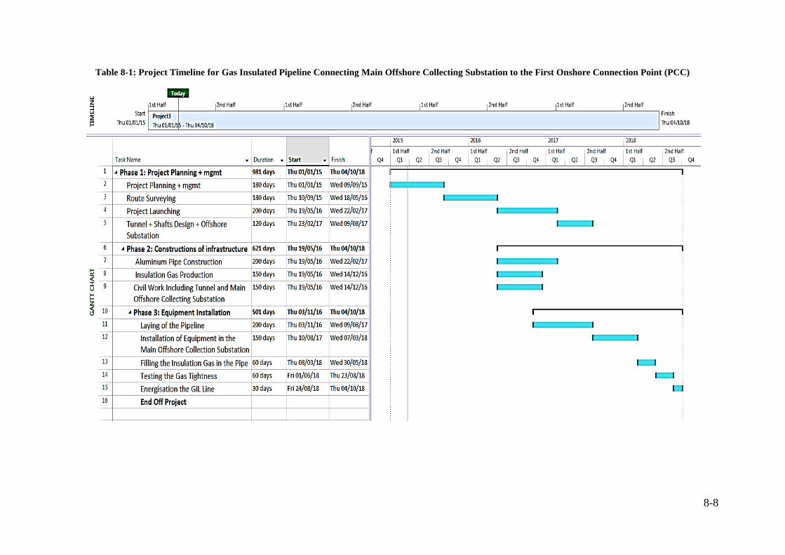
8-8

Table 8-1: Project Timeline for Gas Insulated Pipeline Connecting Main Offshore Collecting Substation to the First Onshore Connection Point (PCC)

8-9

Utilizing GIL as an offshore transmission system requires several wind farms

with high capacity to be combined. This means that a total connection power of

at least 6-8 GW must be achieved. In order to do this, general legal and

regulatory conditions must make it possible not just to connect wind farms

individually but also to take into consideration the future development of offshore

wind farms in an area. If several wind farms are being connected with a single

connection, the connection must be designed in anticipation of future wind farm

developments and be installed before the first wind farm is commissioned.

i

REFERENCES

[1] Roland Berger Strategy Consultants, “Pushing forward: The future of

Offshore Wind Energy.” [Online]. Available:

http://www.rolandberger.co.uk/rbsearch/control/search.html?pid=rbuk_rb_

2332035643&lastWasAdvanced=yes&quickSearch=no&initial=true&quer

yStr=wind&submit.x=16&submit.y=3. [Accessed: 03-Apr-2013].

[2] EWEA, “Wind in power, 2010 european statistics,” 2011. [Online].

Available:

http://www.ewea.org/fileadmin/files/library/publications/statistics/EWEA_

Annual_Statistics_2010.pdf. [Accessed: 05-Apr-2013].

[3] EWEA, “Oceans of opportunity, Harnessing Europe’s largest domestic

energy resource,” 2009. [Online]. Available:

http://www.ewea.org/fileadmin/ewea_documents/documents/publications/r

eports/Offshore_Report_2009.pdf. [Accessed: 07-Jun-2013].

[4] Larsen, Jens HM, Hans Christian Soerensen, Erik Christiansen, Stefan

Naef, and Per Vølund. “Experiences from Middelgrunden 40 MW Offshore

Wind Farm,” Copenhagen offshore Wind Conf. (pp. 1-8)., no. October,

2005.

[5] 4C Offshor, “Forecast of Offshore Wind Foundation Demand in North

West Europe for the Period 2013 -2023,” 2013. [Online]. Available:

http://www.4coffshore.com/windfarms/reports/foundationsReport.aspx.

[6] dena, EWEA, ForWind, IEO, NTUA, Senergy, SINTEF, “Offshore

Electricity Grid Infrastructure in Europe A Techno-Economic

Assessment,” 2011. [Online]. Available:


eports/OffshoreGrid__report.pdf. [Accessed: 28-Feb-2014].

[7] EWEA, “Deep water The next step for offshore wind energy,” 2013.

[Online]. Available:

http://www.ewea.org/fileadmin/files/library/publications/reports/Deep_Wat

er.pdf. [Accessed: 15-Feb-1014].

[8] EWEA, “EU Energy Policy to 2050,” 2011. [Online]. Available:


eports/EWEA_EU_Energy_Policy_to_2050.pdf. [Accessed: 03-Mar-2014].

[9] EWEA, “Wind in our Sails- the coming of european offshore wind energy

industry,” 2011. [Online]. Available:


eports/23420_Offshore_report_web.pdf.

ii

[10] Negra, N. Barberis, Jovan Todorovic, and Thomas Ackermann. “Loss

evaluation of HVAC and HVDC transmission solutions for large offshore

wind farms,” Electric Power Systems Research, 76(11), 916-927. 2006.

[11] Behravesh, Vahid, and Nahid Abbaspour. “New Comparison of HVDC and

HVAC Transmission system,” IJEIR 1, no. 3 (2012): 300-304.

[12] Ackermann, Thomas, Antje Orths, and Krzysztof Rudion." Transmission

Systems for Offshore Wind Power Plants and Operation Planning

Strategies for Offshore Power Systems." Wind Power in Power Systems,

Second Edition (2012): 293-327.

[13] (dena) Deutsche Energie-Agentur GmbH., “dena Grid Study II . Integration

of Renewable Energy Sources in the German Power Supply System from

2015 – 2020 with an Outlook to 2025 .,” 2011. [Online]. Available:

http://www.dena.de/en/publications/energy-system/dena-grid-study-ii.html.

[14] J. Jessus, Rui Castro, J.M. Ferreira,, “HVDC Connection of Offshore Wind

Parks : VSC vs LCC with STATCOM,” in International Conference on

Power Systems Transients (IPST2011)., in Delft., the Netherlands.,.

[15] H. Koch, "Gas-Insulated Transmission Lines (GIL)". Chichester, UK: John

Wiley & Sons, Ltd, 2011.

[16] Takuma, Tadasu, Osamu Yamamoto, and Shoji Hamada. “Gases as a

Dielectric,” In Gaseous Dielectrics X, pp. 195-204. Springer US, 2004.

[17] Koch, H., and A. Schuette. “Gas insulated transmission lines for high

power transmission over long distances,” Electric power systems research

44, no. 1 (1998): 69-74.

[18] Siemens, “Power Engineering Guide, Power Transmission and Distribution

Solutions., Edition 7.0,” [Online]. Available:

http://www.energy.siemens.com/hq/en/energy-topics/publications/power-

engineering-guide/. [Accessed: 19-Feb-2014].

[19] Cigre brochure_218 Joint Working Group 23/21/33.15, “Gas insulated

transmission lines (GIL),” no. February, 2003.

[20] Siemens AG, “International Electrotechnical Commission, Rigid High-

Voltage, Gas-Insulated Transmission Lines for Rated Voltages of 72.5 kV

and above, IEC 61640, IEC,”

[21] Cigre, Working Group B3/B1.09, “Application of Long High Capacity

Gas-Insulated Lines in Structures,” no. October, 2008.

[22] Koch, H., and M. Hopkins. “Overview of gas insulated lines (GIL),” In

Power Engineering Society General Meeting, 2005. IEEE, pp. 940-944.

IEEE.

iii

[23] Baer, Gregor P., A. Diessner, and G. F. Luxa. “420 kV SF6-insulated

tubular bus for the Wehr pumped-storage plant electric tests,” Power

Apparatus and Systems, IEEE Transactions on 95, no. 2 (1976): 469-477.

[24] Schichler, U., A. Diessner, and J. Gorablenkow. “Dielectric on-site testing

of GIL." In Properties and Applications of Dielectric Materials, 2003.

Proceedings of the 7th International Conference on, vol. 1, pp. 15-18.

IEEE.

[25] International Electrotechnical Commission, Rigid High-Voltage, “ Gas-

Insulated Tranmission Lines for Rated Voltages of 72.5 kV and above.",

IEC 61640, IEC, 1998.

[26] Environmental News Service, “Potent New Greenhouse Gas Discovered,”

2000. [Online]. Available: http://www.fluoridealert.org/news/potent-new-

greenhousegas- discovered/. .

[27] Environment News Service, “California Limits SF6, World’s Most Potent

Greenhouse Gas,” 2010. [Online]. Available: http://www.ens-

newswire.com/ens/mar2010/2010-03-02-091.html.

[28] Christophorou, Loucas G., and Richard J. Van Brunt. “SF6/N2 mixtures:

basic and HV insulation properties,” Dielectrics and Electrical Insulation,

IEEE Transactions on 2, no. 5 (1995): 952-1003.

[29] Christophorou, Loucas G., James Kenneth Olthoff, and David S. Green.

“Gases for Electrical Insulation and Arc Interruption: Possible Present and

FutureAlternatives to Pure SF6,” National Instutute of Standards and

Technology (NIST), U.S. Department of Commerce, Washington, USA,

November, 1997.

[30] Marsden, H. I., M. D. Hopkins, and C. R. Eck III. “Lightning Impulse

Withstand Performance of a Practical GIC With 5 and 10 Percent SF6/N2

Mixtures,”. In Electrical Insulation, 1998, Conference Record of the 1998

IEEE International Symposium on, vol. 2, pp. 710-713. IEEE, 1998.

[31] Boeck, W., W. Taschner, J. Gorablenkow, G. F. Luxa, and L. Menten.

“Insulating behaviour of SF6 without solid insulation in case of fast

transients,” CIGRE paper 15-07 (1986).

[32] Qiu, Y., and Y. P. Feng. “Investigation of SF6-N2, SF6-CO2 and SF6-Air

as Substitutes for SF6 Insulation,” In Electrical Insulation, 1996.,

Conference Record of the 1996 IEEE International Symposium on, vol. 2,

pp. 766-769. IEEE.

[33] Koch Hermann. “Experience with 2nd Generation Gas-Insulated

Transmission Lines GIL,” In World Energy Transmission System

Workshop, Meudon, France., 2003.

iv

[34] Koch Hermann, A. Schuette. “Gas insulated transmission lines for high

power transmission over long distances,” Electric Power Systems

Research, 44, no. 1 (1998): 69-74.

[35] Koch Hermann, and Thomas Hillers. “Second generation gas-insulated

line,” Power Engineering Journal 16, no. 3 (2002): 111-116.

[36] Henningsen, C. G., G. Kaul, H. Koch, A. Schuette, and R. Plath “Electrical

and Mechanical Long-Time Behaviour of Gas-Insulated Transmission

Lines,” In CIGRE Session (Vol. 8, p. 2000), Paris.

[37] Koch Hermann. “N2/SF6 gas-insulated line of a new GIL generation in

service", CIGRE Session, Paris, 08/2002.”

[38] United Nations, “KYOTO PROTOCOL TO THE UNITED NATIONS

FRAMEWORK KYOTO PROTOCOL TO THE UNITED NATIONS

FRAMEWORK,” 1998. [Online]. Available:

http://unfccc.int/resource/docs/convkp/kpeng.pdf.

[39] Qiu, Y., and E. Kuffel. “‘Comparison of SF6/N2 and SF6/CO2 Gas

Mixtures as Alternatives to SF6 Gas,’ Dielectrics and Electrical Insulation,


[40] MUHAMMAD SAUFI KAMARUDIN, “Experimental Investigation of

CF3I-CO2 Gas Mixtures on the Breakdown Characteristics in Uniform and

Nonuniform Field Configurations,” School of Engineering Cardiff

University, 2013.

[41] Hikita, Masayuki, Shinya Ohtsuka, Shigemitsu Okabe, and Genyo Ueta.

“Breakdown Mechanism in C3F8/CO2 Gas Mixture under Non-uniform

Field on the Basis of Partial Discharge Properties,” Dielectrics and

Electrical Insulation, IEEE Transactions on 16, no. 5 (2009): 1413-1419.

[42] Qiu, X. Q., I. D. Chalmers, and P. Coventry. “A study of alternative

insulating gases to SF6,” Journal of Physics D: Applied Physics 32, no. 22

(1999): 2918.

[43] ISO/DIS 14520-12, “Gaseous media fire extinguishing systems — Physical

properties and system design — Part 2: CF3I Extinguishant,” 2013.


http://www.iso.org/iso/home/store/catalogue_tc/catalogue_detail.htm?csnu

mber=55348&commid=46628.

[44] Taki, M., D. Maekawa, H. Odaka, H. Mizoguchi, and S. Yanabu.

“Interruption capability of CF/sub 3/I Gas as a substitution candidate for

SF/sub 6/ gas,” Dielectrics and Electrical Insulation, IEEE Transactions

on 14, no. 2 (2007): 341-346.

[45] Toyota, Hiroyuki, Shigeyasu Matsuoka, and Kunihiko Hidaka.

“Measurement of sparkover voltage and time lag characteristics in CF3I–

v

N2 and CF3I– air gas mixtures by using steep-front square voltage,” IEEJ

Transactions on Fundamentals and Materials 125 (2005): 409-414.

[46] Mohamad Kamarol bin Mohd Jamil., “Partial Discharge Properties and Gas

Decomposition Analysis of Environmental Friendly Gas Insulation Media

as a Basis of Diagnostic Technique Development,” Department of

Electrical and Electronic Engineering Graduate School of Engineering

Kyushu Institute of Technology,, 2007.

[47] Katagiri, H., H. Kasuya, H. Mizoguchi, and S. Yanabu. “Investigation of

the performance of CF3I Gas as a Possible Substitute for SF6,” Dielectrics

and Electrical Insulation, IEEE Transactions on 15, no. 5 (2008): 1424-

1429.

[48] IEC 62271-204, “High-voltage switchgear and controlgear – Part 204:

Rigid gas-insulated transmission lines for rated voltage above 52 kV, IEC,

Geneva, Switzerland,” 2011.

[49] Volcker, O., and H. Koch. “Insulation Co-ordination for Gas-Insulated

Transmission Lines ( GIL )", In Power Engineering Society Winter

Meeting, 2000, IEEE, vol. 1, pp. 703-711. IEEE.

[50] Chakravorti, S., and H. Steinbigler. “Capacitive-resistive field calculation

on HV bushings using the boundaryelement method", Dielectrics and

Electrical Insulation, IEEE Transactions on 5, no. 2 (1998): 237-244.

[51] Kuffel, John, E. Kuffel, and Walter S. Zaengl. High Voltage Engineering

Fundamentals., Second edition, Newnes, 2000.

[52] IEC 62271-1 ed1.0, “High-voltage switchgear and controlgear – Part 1:

Common specifications, IEC, Geneva, Switzerland, 2007-10.” .

[53] EN 50068., “Wrought steel enclosures for gas-filled high-voltage

switchgear and controlgear, IEC, Geneva, Switzerland 1991.,” no. 1, 1991.

[54] Cigre Working Group 21/23/33-02, “Insulation co-ordination of 420 kV

gas insulated lines (GIL),” 1998.

[55] Kuroyanagi, Y., A. Toya, T. Hayashi, and T. Araki. “Construction of

8000A class 275 kV gas insulated transmission line,” Power Delivery,


[56] Babusci B., Colombo E., Speziali. “Assessment of the behaviour of gas-

insulated electrical components in the presence of an internal arc,” ENEL

Research, CIGRE Session, Paris, France,, 1998.

[57] Henningsen, C. G., G. Kaul, H. Koch, A. Schuette, and R. Plath.

“Electrical and Mechanical Long- Time Behaviour of Gas-Insulated

Transmission Lines,” In CIGRE Session, vol. 8, p. 2000. 2000.

vi

[58] Minaguchi, D., M. Ginno, K. Itaka, H. Furukawa, K. Ninomiya, and T.

Hayashi. “Heat Transfer Characteristics of Gas-Insulated Transmission

Lines,” Power Delivery, IEEE Transactions on 1, no. 1 (1986): 1-9.

[59] Itaka, Koshi, Tomoo Araki, and Takushi Hara. “Heat Transfer

Characteristics of Gas Spacer Cables,” Power Apparatus and Systems,

IEEE Transactions on 5 (1978): 1579-1585.

[60] Chakir, A., and H. Koch. “Turbulent Natural Convection and Thermal

Behaviour of Cylindrical Gas-Insulated Transmission Lines ( GIL ),” In

Power Engineering Society Summer Meeting, 2001, vol. 1, pp. 162-167.

IEEE, 2001.

[61] Chakir, Abdellah, Y. Sofiane, Nicolas Aquelet, and Mhamed Souli. “Long

term test of buried gas insulated transmission lines (GIL),” Applied thermal

engineering 23, no. 13 (2003): 1681-1696.

[62] Koch, H., and A. Chakir. “Thermal calculation for buried Gas-Insulated

Transmission Lines (GIL) and XLPE-cable,” In Power Engineering Society

Winter Meeting, 2001. IEEE, vol. 2, pp. 857-862. IEEE.

[63] McDonald, John D., ed. “ElECTRIC POWER SUBSTATIONS

ENGINEERING.” CRC press, 2012.

[64] Henningsen, C. G., G. Kaul, H. Koch, A. Schuette, and R. Plath.

“Electrical and mechanical long time behaviour of gas-insulated

transmission lines,” In CIGRE Session, vol. 8, p. 2000. 2000.

[65] Cigre SESSION B1-103_2004, “New generation of GIL -Characteristics

and applications,” 2004.

[66] Poehler, S.; Rudenko, P., “Directly Buried Gas-Insulated Transmission,”

Transmission and Distribution Conference and Exposition (T&D), 2012

IEEE PES , vol., no., pp.1,5, 7-10 May 2012

[67] Siemens AG, “GIL – high-power transmission technology.” [Online].

Available: http://www.energy.siemens.com/hq/pool/hq/power-

transmission/gas-insulated-transmission-lines/GIL_e.pdf. [Accessed: 15-

May-2012].

[68] Radiation International and Association Protection., “Human Exposure to

Electromagnetic Fields,” 2009. [Online]. Available: http://www.irpa.net/.

[69] Health and Safety Ececutive, “Radiation Home,” 2010. [Online].

Available: http://www.hse.gov.uk/radiation/ionising/doses/. [Accessed: 03-

Sep-2013].

[70] Siemens AG, “Undergrounding Electricity Transmission: Introduction to

Gas Insulated Line (GIL) technology,” National Symposium on Future

Electricity Networks, ICE,. 2011.

vii

[71] Chakir, Abdellah, and Hermann Koch. “Corrosion protection for gas-

insulated transmission lines,” In Power Engineering Society Summer

Meeting, 2002 IEEE, vol. 1, pp. 220-224. IEEE, 2002.

[72] Koch H, “Preferential Subject D1 PS2 Q6: Is there any experience from the

application in the field of N2/SF6 mixtures and especially in high voltage

Gas-Insulated Lines?,” CIGRE Session 2004, Paris, 08/2004.

[73] Miyazaki, Akinobu, Manabu Yagi, S-I. Kobayashi, C. Min, K. Hirotsu, and

H. Nishima. “Development of partial discharge automated locating system

for power cable,” In Electrical Insulation and Dielectric Phenomena, 1998.

Annual Report. Conference on, pp. 424-427. IEEE, 1998.

[74] Okubo, H., M. Yoshida, T. Takahashi, T. Hoshino, M. Hikita, and A.

Miyazaki. “Partial Discharge Measurement in a Long Distance SF6 Gas

Insulated,” Power Delivery, IEEE Transactions on 13, no. 3 (1998): 683-

690.

[75] Hoshino, Toshihiro, Hiroshi Koyama, Shiro Maruyama, and Masahiro

Hanai. “Comparison of Sensitivity Between UHF Method and IEC 60270

for Onsite Calibration in Various GIS,” Power Delivery, IEEE

Transactions on 21, no. 4 (2006): 1948-1953.

[76] Orlando P. Hevia., “Alternative Transients Program - Comparison of

transmission line models.” [Online]. Available: http://iitree-

unlp.org.ar/caue/Archivos/emodlin.pdf.

[77] Dommel. Hermann W, Electromagnetic Transients Program: Reference

Manual:(EMTP theory book). Bonneville Power Administration,, 1986.

[78] CGIT Westboro., “Compressed Gas Insulated Transmission Bus Systems

Proven Solutions.” [Online]. Available:

http://www.azz.com/sites/default/files/documents/CGIT.pdf. [Accessed:

01-Mar-2011].

[79] A. Juan, Martinez-Velasco, Ed., Power systems transients :parameter

determination, 1st ed. CRC Press Taylor & Francis Group, 2010.

[80] Gustavsen, Bjørn. “Panel Session on Data for Modeling System Transients

Insulated Cables,” In Power Engineering Society Winter Meeting, 2001.

IEEE, vol. 2, pp. 718-723. IEEE, 2001.

[81] Gudmundsdottir, Unnur Stella, Bjørn Gustavsen, Claus Leth Bak, and

Wojciech Wiechowski. “Field Test and Simulation of a 400 kV Cross-

Bonded Cable System,” Power Delivery, IEEE Transactions on 26, no. 3

(2011): 1403-1410.

[82] BS EN, “Conductors of insulated cables,. BS EN 60228:2005.” .

viii

[83] ABB, “XLPE Land Cable Systems User ´ s Guide.” [Online]. Available:

http://www.elektroskandia.ee/pub/tooted/keskpinge-korgepinge/XLPE-

Land-Cable-Systems-2GM5007GB-rev-5.pdf. [Accessed: 03-Mar-2012].

[84] ABB, “XLPE Submarine Cable Systems Attachment to XLPE Land Cable

Systems - User ´ s Guide.” [Online]. Available:

http://www04.abb.com/global/seitp/seitp202.nsf/0/badf833d6cb8d46dc125

7c0b002b3702/$file/XLPE+Submarine+Cable+Systems+2GM5007+.pdf#

page=1&zoom=auto,0,814. [Accessed: 03-Mar-2012].

[85] National Grid, “Electric and Magnetic Fields ‘Geometries for calculating

fields from power lines.’”[Online]. Available:

http://www.emfs.info/Sources+of+EMFs/Overhead+power+lines/Calculati

ng/geometries/. [Accessed: 05-Apr-2012].

[86] Nasser D. Tleis, Power Systems Modelling and Fault Analysis Theory and

Practice. Elsevier Ltd., 2008.

[87] CIGRE WG 33.02, “Guidelines for representation of network elements

when calculating transients,” CIGRE Rep. no. 39.,, 2000.

[88] Alternative Transient Program (ATP) Rule Book. .

[89] Schlabbach, Jürgen, and Karl-Heinz Rofalski. Power System Engineering

Planning, Design, and Operation of Power Systems and Equipment. John

Wiley & Sons, 2008.

[90] Institute of Electrical and Electronics Engineers, “IEEE Application Guide

for AC High-Voltage Circuit Breakers Rated on a Symmetrical Current

Basis,” IEEE Std C37.010-1999. p. i, 2000.

[91] Martinez, Jorge, P. C. Kjar, Pedro Rodriguez, and Remus Teodorescu.

“Short circuit signatures from different wind turbine generator types,” In

Power Systems Conference and Exposition (PSCE), 2011 IEEE/PES, pp. 1-

7. IEEE, 2011.

[92] Kanellos, F. D., and John Kabouris. “Wind farms modeling for short-

circuit level calculations in large power systems,” Power Delivery, IEEE

Transactions on 24, no. 3 (2009): 1687-1695.

[93] IEC 60909-0, “Short-circuit currents in three-phase a.c. systems - Part 0:

Calculation of currents.” 2001.

[94] Samaan, Nader, Robert Zavadil, J. Charles Smith, and Jose Conto.

“Modeling of wind power plants for short circuit analysis in the

transmission network,” In Transmission and Distribution Conference and

Exposition, 2008. T&D x00026; D. IEEE/PES, pp. 1-7. IEEE, 2008.

[95] Muljadi, E., C. P. Butterfield, A. Ellis, J. Mechenbier, J. Hochheimer, R.

Young, N. Miller, R. Delmerico, R. Zavadil, and J. C. Smith.

ix

“Equivalencing the collector system of a large wind power plant,” In

Power Engineering Society General Meeting, 2006. IEEE, pp. 9-pp. IEEE,

2006.

[96] Martinez, J. A., J. Mahseredjian, and B. Khodabakhchian. “Parameter

Determination for Modeling System Transients — Part VI : Circuit

Breakers,” Power Delivery, IEEE Transactions on 20, no. 3 (2005): 2079-

2085.

[97] HOTA, BHABANI SANKAR. “LOAD FLOW STUDY IN POWER

SYSTEM,” Doctoral dissertation, Department of Electrical Engineering

National Institute of Technology, 2011.

[98] EPRI, “Increased Power Flow Through Transmission Circuits : Overhead

Line Case Studies and Quasi-Dynamic Rating,” vol. 3, no. 3, 2006.

[99] CLAIR, HPST. “Practical Concepts in Capability and Performance of

Transmission Lines,” Power Apparatus and Systems, Part III. Transactions

of the American Institute of Electrical Engineers, vol. 72, no.2,, pp. 1152–

1157, 1953.

[100] Gutman, Richard, P. P. Marchenko, and R. D. Dunlop. “Analytical

Development of Loadability Characteristics for EHV and UHV

Transmission Lines,” Power Apparatus and Systems, IEEE Transactions

on 2 (1979): 606-617.

[101] National Grid, “National Electricity Transmission System Security and

Quality of Supply Standard,” 2012.

[102] Colla, L., F. M. Gatta, A. Geri, S. Lauria, and M. Maccioni. “Steady-state

operation of very long EHV AC cable lines,” In PowerTech, 2009 IEEE

Bucharest, pp. 1-8. IEEE, 2009.

[103] Gatta, F. M., and S. Lauria. “Very long EHV cables and mixed overhead-

cable lines. Steady-state operation,” In Power Tech, 2005 IEEE Russia, pp.

1-7. IEEE, 2005.

[104] Gatta, F. M., A. Geri, S. Lauria, and M. Maccioni. “Steady-state operating

conditions of very long EHVAC cable lines: Two case studies,” Electric

Power Systems Research 83, no. 1 (2012): 160-169.

[105] John J. Grainger, WUliam D. Stevenson, POWER SYSTEM ANALYSIS.

McGraw-Hill, Inc.,, 1994.

[106] IEC 60071-1, “Insulation Co-ordination Part 1: Definitions. Principles and

Rules.” 2006.

[107] “IEC 60071-1, ‘Insulation Co-ordination Part 2: Application Guide,’

1996.”.

x

[108] A report by the European Wind Energy Association, “Wind in our Sails,

The coming of Europe’s offshore wind energy industry,” 2011. [Online].

Available:


eports/23420_Offshore_report_web.pdf.

[109] Yu, Cunyi, Nit Petcharaks, and Chairoj Panprommin. “The statistical

calculation of energization overvoltages, case of EGAT 500 kV lines,” In

Power Engineering Society Winter Meeting, 2000. IEEE, vol. 4, pp. 2705-

2709. IEEE, 2000.

[110] Marzinotto, M., C. Mazzetti, and P. Schiaffino. “Statistical approach to the

insulation coordination of medium and high voltage cable lines,” In Power

Tech, 2005 IEEE Russia, pp. 1-8. IEEE, 2005.

[111] Thomas, Mini S., C. S. Indulkar, and P. R. Bijwe. “Sensitivity analysis of

peak switching overvoltages in underground cables,” Electric Machines

and Power Systems 16, no. 5 (1989): 331-342.

[112] “IEC 60071-1, “Insulation Co-ordination-part 2: Application guide, IEC

STD 60071-2.3. Technical report, IEC, 1996.” .

[113] National Grid, “Seven Year Statement 2010 (SYS), Appendix D.”


http://www.nationalgrid.com/uk/Electricity/SYS/current/. [Accessed: 19-

Apr-2012].

[114] da Silva, Filipe Miguel Faria. “Analysis and simulation of electromagnetic

transients in HVAC cable transmission grids,” PhD diss., Videnbasen for

Aalborg UniversitetVBN, Aalborg UniversitetAalborg University, Det

Teknisk-Naturvidenskabelige FakultetThe Faculty of Engineering and

Science, Elektriske anlægElectric Power Systems, 2011.

[115] Ohno, T., A. Ametani, C. L. Bak, W. Wiechowski, and T. K. Sørensen.

“Analysis of the Statistical Distribution of Energization Overvoltages of

EHV Cables and OHLs,” 2013.

[116] King, R., F. Moore, N. Jenkins, A. Haddad, H. Griffiths, and M. Osborne.,

“Switching Transients in Offshore Wind Farms–Impact on the Offshore

and Onshore Networks.” IPST, Delft, the Netherlands (2011).

[117] Johansson, Stefan G., J. Hanson, J. Karlström, F. Krogh, and L. Liljestrand

“AC Cable solutions for Offshore Wind Energy,” In Copenhagen Offshore

Wind Conference., pp. 1–10, 2005.

[118] WindTECH International, “PTP Goes Offshore.” [Online]. Available:

http://www.windtech-international.com/articles/ptp-goes-offshore.

[Accessed: 10-Mar-2013].

xi

[119] Kyriakides, Stelios, and Edmundo Corona, “Mechanics of offshore

pipelines: volume 1 buckling and collapse. Vol. 1.” Elsevier,, 2007.

[120] Chakrabarti, Subrata, “Handbook of Offshore Engineering (2-volume set).

Vol. 1.” Elsevier,, 2005.

[121] Forwind., “Dogger Bank Project One Environmental Impact Assessment

Scoping Report,” 2010. [Online]. Available:

http://www.forewind.co.uk/uploads/files/project-one-scoping-report.pdf.

[Accessed: 20-Nov-2013].

[122] ForWind, E.U. Commission of European Transmission Networks

Electricity, “Broshure Grid Connection of Offshore Wind Farms – A

Feasibility Study on the Application of Power Transmission Pipelines

(PTP®),” 2005. [Online]. Available:

http://www.forwind.de/forwind/index.php?article_id=306&clang=1.

[123] ICES, “International Council for the Exploration of the Sea (ICES).”


https://www.google.co.uk/webhp?tab=ww&ei=zfx2VJyGDMb4UtzKgegJ

&ved=0CAYQ1S4#q=+International+Council+for+the+Exploration+of+th

e+Sea+%28ICES%29. [Accessed: 02-Mar-2014].

[124] “Prysmian Cable and System. High Voltage Cables.” [Online]. Available:

www.prysmian.nl/export/sites/prysmian-nlNL/.../Prysmian_HVC_LR.pdf.

[Accessed: 02-Aug-2012].

[125] ABB, “XLPE Cable Systems User ´ s guide,” pp. 1–32.

[126] R. Nick, Barton, TBM tunnelling in jointed and faulted rock. CRC Press,

2000.

[127] W. Leader, I. N. Large, and D. Pipe, “WORLD LEADER IN LARGE

DIAMETER PIPE MANUFACTURING POLYETHYLENE,” no. 510.

[128] ForWind, Siemens, ILF Consultaing Engineers, “Feasibility Study for

Large-Scale Grid Connection of Remote Offshore Wind Energy.” [Online].

Available:

http://www.forwind.de/forwind/index.php?article_id=61&clang=1.

[129] Carbon Trust, “Offshore wind power: big challenge, big opportunity.”


http://www.carbontrust.com/resources/reports/technology/offshore-wind-

power.

[130] Danielle Lane., “THE CROWN ESTATE Round 3 Offshore Wind Farm

Connection Study Version 1.0,” A report by Senergy Econnect and

National Grid for the Crown Estate. .

xii

[131] Madariaga, A., I. Martínez de Alegría, J. L. Martín, P. Eguía, and S.

Ceballos. “Current facts about offshore wind farms,” Renewable and

Sustainable Energy Reviews 16, no. 5 (2012): 3105-3116.

[132] Parsons Brinckerhoff and Institution of Engineering and Technology,

“electricity transmission costing study,” 2012. [Online]. Available:

http://www.theiet.org/factfiles/transmission-report.cfm. [Accessed: 06-

Nov-2013].

[133] ENTSOE, “Offshore Transmission Technology,” PREPARED BY THE

REGIONAL GROUP NORTH SEA FOR THE NSCOGI (NORTH SEAS

COUNTRIES‟ OFFSHORE GRID INITIATIVE), 2011. .

[134] National Grid., “Electricity Transmission Cost Study: How does the

independent report compare to National Grid’s view?,” no. February, pp.

1–3, 2012.

[135] T. A. Moore., S. R. Skaggs., M. R. Corbitt., R. E. Tapscott., D. S.

Dierdorf., and C. j. Kibert., “No TitleThe Development of CF3I as a Halon

Replacement.,” The University of New Mexico, 1994. .

[136] Charles J. Kibert., “Fluoroiodocarbons as Halon 1211 / 1301

Replacements : An Overview,” Wright Laboratory, U.S. Air Force. .

[137] K. S. and R. B. B. Van Eeckhout, D. Van Hetem, M. Reza, “Economic

comparison of VSC HVDC and HVAC as transmission system for a 300

MW offshore wind farm,” European Transactions on Electrical Power, no.

June 2009, pp. 661–671, 2010.

[138] ABB., “It’s time to connect with offshore wind supplement,” 2010.


http://www05.abb.com/global/scot/scot221.nsf/veritydisplay/1bad1970cd0

766eec1257b28005757df/$file/Pow0038 R6 LR.pdf. [Accessed: 09-Dec-

2013].

xiii

APPENDIX 1: List of Abbreviations

HVAC

HVDC

GIL

GIS

EMTP

EU

EHV

XLPE

LCC-CSC

VSC

PCC

IGBT

pu

SF6

CF3I

EDF

GWP

C

F

ODP

SYS

LIWV

SIWV

PFWV

IRPA

PE

PP

IEC

CIGRE

High Voltage Alternate Current

High Voltage Direct Current

Gas-Insulate Transmission Line

Gas Insulated Substation/Switchgear

Electromagnetic Transient Program

European Union

Extra High Voltage

Cross-Linked Polyethylene

Line-Commutated Current Source Converters

Voltage Source Converters

Point of Common Coupling

Insulation Gate Bipolar Transistors

Per unit

Sulphur Hexafluoride

Trifluoroiodomethane

Electrical De France

Global Warming Potential

Carbon

Fluorine

Ozone Depleting Potential

Seven Year Statement

Lightning Impulse Withstand Voltage

Switching Impulse Withstand Voltage

Power Frequency Withstand Voltage

International Radiation Protection Association

Polyethylene

Polypropylene

International Electrotechnical Commission

International Council on Large Electric Systems

ii

Appendix 2: Existing GIL Projects

Examples of Existing GIL Projects [2] Examples of existing GIL Projects (1)

OWNER Energie Ouest

Suisse

RWE Net Chubu electric power

company

DATE OF

COMMISSIONING

2001 1975 1998

INSTALLATION

PLACE

GENEVA,

Switzerland

WEHR, Germany SHINMEIKATOKAI,

Japan

TYPE OF

INSTALLATION

TUNNEL TUNNEL TUNNEL

LENGTH OF LINK 420 m 670 m 3300 m

NUMBER OF

SYSTEMS

2 2 2

NOMINAL VOLTAGE

OF NETWORK

220 kV 380 kV 275 kV

HIGHEST VOLTAGE

FOR EQUIPMENT

300 kV 420 kV 300 kV

RATED CURRENT

PERSYSTEM

2000 A 2500 A 6300 A

INSULATING GAS

7 bar abs 4.9 bar abs 5.4 bar abs

20% SF6 / 80% N2 100% SF6 100% SF6

CONDUCTOR

OUTER DIAMETER

(mm)

180

150

170

WALL THICKNESS

(mm)

5

5

20

MATERIAL

Al alloy

EN AW 6101B

E-Al/MgSi0,5 T6

W19

E-ALMgSi0,5

Al alloy

IACS*

61 % 48-54 % 59.5 %

CONDUCTIVITY at

20oC

m/Ω.mm2

35.3857 27.84-31.32 34.518

RESISTIVITY at 20oC

m/Ω.mm2

0.02826 0.032-0.036 0.02897

ENCLOSURE

INNER DIAMETER 500 520 460

WALL THICKNESS 6 5 10

iii

*IACS = International Annealed Copper Standard (IACS=100 % ⇒ Copper Standard

Conductivity = 58,108 m/Ω⋅mm2)

Examples of existing GIL Projects (2)

OWNER National Grid

UK

Entergy BC Hydro

DATE OF

COMMISSIONING

2004 2001 1981

INSTALLATION PLACE Hams Hall, United

Kingdom

Baxter Wilson Power

Plant

USA

Revel stoke Hydro

Power Plant

Canada

TYPE OF

INSTALLATION

Above Ground /

Trench

Above Ground TUNNEL

LENGTH OF LINK 545 m 1250 m 400 m

NUMBER OF SYSTEMS 1 1 2

NOMINAL VOLTAGE

OF

NETWORK

400 kV 500 kV 500 kV

HIGHEST VOLTAGE

FOR

EQUIPMENT

420 kV 550 kV 550 kV

RATED CURRENT PER

SYSTEM

4000 A 4500 A 4000 A

INSULATING GAS 10.3 bar abs 3.79 bar abs 3.45 bar abs

20% SF6 / 80% N2 100% SF6 100% SF6

CONDUCTOR

OUTER DIAMETER

(mm)

512-520 178 178

WALL THICKNESS

(mm)

12.7 12.7 12.7

MATERIAL Al alloy

Al alloy

6061-T6

Al alloy

6061-T6

IACS*

- 59.5 % 59.5 %

CONDUCTIVITY at 20oC

m/Ω.mm2

- 34.57 % 34.57 %

RESISTIVITY at 20oC

m/Ω.mm2

- 0.0289 0.0289

ENCLOSURE

INNER DIAMETER 500 508 508

WALL THICKNESS 6-10 6.35 6.35

*IACS = International Annealed Copper Standard (IACS=100 % ⇒ Copper Standard

Conductivity = 58,108 m/Ω⋅mm2)

iv

Appendix 3: Physical Properties of CF3I Gas

Physical Properties of CF3I [3] Physical or Chemistry Property Value or Description

Molecular weight 195.1

Physical state at 20°C Gas

Melting point – 110°C (– 166°F)

Boiling point at 1 atm – 22.5°C (– 8.5°F)

Liquid density at – 32.5°C 2.36 g/mL

Odour threshold Odourless

Solubility in water Slight

Vapour pressure at 25°C 78.4 psia

Pressure-temperature curve log psia = 5.7411-1146.82/T/K

Critical pressure 586 psia (estimated)

Critical temperature 122°C (estimated)

Critical volume 225 cm3/mole (estimated)

Electron affinity 150 ± 20 kJ/mole 150 ± 20 kJ/mole

Vapour heat capacity 16.9 cal/mole-K

C-I bond dissociation energy 54 kcal/mole

Vapour density (air = 1) 6.9

v

Appendix 4: GIL Electrical Parameters

GIL Inductance “l”

The inductance per unit length can be calculated by considering the typical

coaxial structure of a GIL as shown in Figure 1 where R1, R2 are the phase

inner and outer radius and R3, R4 the enclosure inner and outer radius

respectively [2], [4].

Where 𝜇0 → Magnetic permeability of free space = 2𝜋 ∗ 10−7 H/m

𝑙 = μ0

2πln

R3

R2 [H/m]

Figure 1: coaxial structure of a GIL

GIL Capacitance “C”

The capacitance per unit length can be computed considering the cylindrical

symmetry and the permittivity of the gas mixture 휀0 = 8.854 ∗ 10−12 F/m.

Since the nitrogen is 80% of the gas mixture, so then the permittivity considered

(as for the free space). R3 and R2 are shown in figure 2 [2],[4].

𝐶 =2𝜋𝜀0

ln𝑅3𝑅2

[F/m]

vi

GIL Resistance “r”

The resistance r per unit length depends on the conductor and enclosure

dimensions and electrical resistivity, where the skin and proximity effects of the

conductor and enclosure are negligible [2], [4].

r = rph + ren [Ω/km]

rph = ρph

Sph [Ω/km]

Where ρph is expressed in [Ω mm2/km] and it must be evaluated at the operation

temperature and Sph is the cross section area. R1,R2, R3 and R4 are shown in fig

1.

Sph = π ∗ (R22 − R1

2) [mm2]

For the enclosure

ren = ρen

Sen [Ω/km]

Sen = π ∗ (R42 − R3

2) [mm2]

GIL Surge Impedance

𝑍0 =1

2𝜋ln

𝑅3

𝑅2√

𝜇𝑜

휀𝑜

vii

Appendix 5: MTLAP Equations for Long Transmission Line

R=8.616e-3;

l=2.05e-4;

c=54.2e-9;

f=50;

l=j*2*pi*f*l;

𝑧 = 𝑅 + 𝑙 y=j*2*pi*f*c

Zc = sqrt (z/y);

ga = sqrt(z ∗ y);

L1= [0:50:500];

L2= [0:50:400];

L3= [0:50:300];

L4= [0:50:200];

B1= Zc.∗ sinh(L1.∗ ga); B2= Zc.∗ sinh(L2.∗ ga); B3= Zc.∗ sinh(L3.∗ ga); B4= Zc.∗ sinh(L4.∗ ga); A1= cosh(L1.∗ ga); A2= cosh(L2.∗ ga); A3= cosh(L3.∗ ga); A4= cosh(L4.∗ ga); C1= (sinh(L1.∗ ga))./Zc; C2= (sinh(L2.∗ ga))./Zc; C3= (sinh(L3.∗ ga))./Zc; C4= (sinh(L4.∗ ga))./Zc; Vs=complex (342928.6,0);

Is1=complex (2938.838,-1120.535);

Is2=complex (3048.19,-1415.391);

Is3=complex (3181.1768,-1708.13578);

Is4=complex (3327.33369,-1999.885);

Vr1= (A1.*Vs)-(B1.*Is1);

Vr2= (A2.*Vs)-(B2.*Is2);

Vr3= (A3.*Vs)-(B3.*Is3);

Vr4= (A4.*Vs)-(B4.*Is4);

V1=abs (Vr1);

V2=abs (Vr2);

V3=abs (Vr3);

V4=abs (Vr4);

Plot (L1, V1,'b', L2, V2,'g', L3, V3,'r', L4, V4)

Ir1= (A1.*Is1)-(C1.*Vs);

Ir2= (A2.*Is2)-(C2.*Vs);

Ir3= (A3.*Is3)-(C3.*Vs);

Ir4= (A4.*Is4)-(C4.*Vs);

I1=abs (Ir1);

I2=abs (Ir2);

I3=abs (Ir3);

viii

I4=abs (Ir4);

Plot (L1, I1,'b', L2, I2,'g', L3, I3,'r', L4, I4)

thV1=angle (Vr1);

thV2=angle (Vr2);

thV3=angle (Vr3);

thV4=angle (Vr4);

thI1=angle (Ir1);

thI2=angle (Ir2);

thI3=angle (Ir3);

thI4=angle (Ir4);

V1=V1. /sqrt (2);

V2=V2. /sqrt (2);

V3=V3. /sqrt (2);

V4=V4. /sqrt (2);

I1/I1. / sqrt (2);

I2/I2. / sqrt (2);

I3/I3. / sqrt (2);

I4/I4. / 𝑠𝑞𝑟𝑡 (2);

P1= (V1.*I1).*cos (thV1-thI1);




Plot (L1, P1,'b', L2, P2,'g', L3, P3,'r', L4, P4)

Q1= (V1.*I1).*sin (thV1-thI1);




Plot (L1, Q1,'b', L2, Q2,'g', L3, Q3,'r', L4, Q4)

REFERENCES for APPENDIXES:

1. EWEA., “Wind in our Sails- the coming of european offshore wind energy

industry,” 2011. [Online].

Available:http://www.ewea.org/fileadmin/ewea_documents/documents/pu

blications/reports/23420_Offshore_report_web.pdf

2. Cigre, Working Group B3/B1.09, “Application of Long High Capacity

Gas-Insulated Lines in Structures,” no. October, 2008.

3. Subcommittee on Iodotrifluoromethane, Committee on Toxicology, Board

on Environmental Studies and Toxicology, and Division on Earth and Life

Studies, “Iodotrifluoromethane: Toxicity Review,” Washington, D.C.

Natl. Acad. Press. Press., 2004.

4. Cigre brochure_218 Joint Working Group 23/21/33.15, “Gas insulated

transmission lines (GIL),” no. February, 2003.

Documents

Evaluation of Gas Insulated Lines (GIL) for Long Distance ...orca.cf.ac.uk/73315/1/2015ElnaddabKPhD.pdf · Evaluation of Gas Insulated Lines ... using an HVAC gas-insulated transmission