Evaluation of hydrodynamic dispersion parameters in ... · Evaluation of hydrodynamic dispersion parameters in fractured rocks ... equivalent porous media of fracture networks)

$Page 1: Evaluation of hydrodynamic dispersion parameters in ... · Evaluation of hydrodynamic dispersion parameters in fractured rocks ... equivalent porous media of fracture networks)$
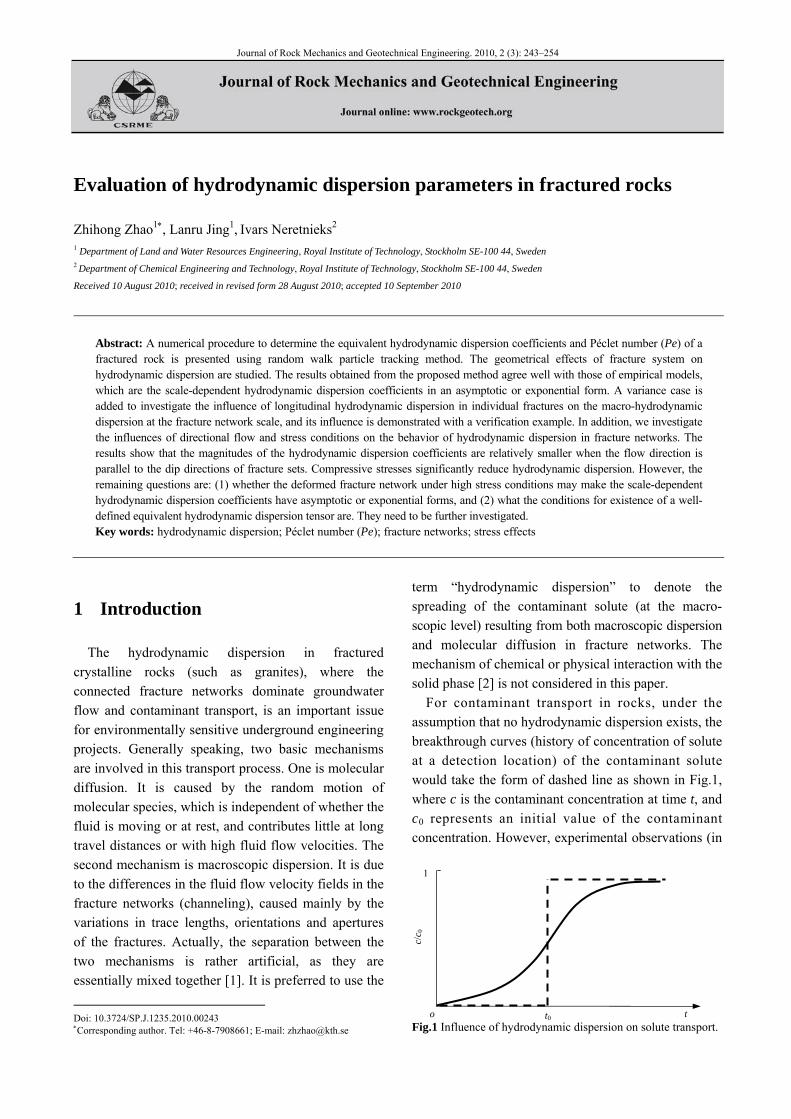
Journal of Rock Mechanics and Geotechnical Engineering. 2010, 2 (3): 243–254

Evaluation of hydrodynamic dispersion parameters in fractured rocks

Zhihong Zhao1, Lanru Jing1, Ivars Neretnieks2 1 Department of Land and Water Resources Engineering, Royal Institute of Technology, Stockholm SE-100 44, Sweden 2 Department of Chemical Engineering and Technology, Royal Institute of Technology, Stockholm SE-100 44, Sweden

Received 10 August 2010; received in revised form 28 August 2010; accepted 10 September 2010

Abstract: A numerical procedure to determine the equivalent hydrodynamic dispersion coefficients and Péclet number (Pe) of a fractured rock is presented using random walk particle tracking method. The geometrical effects of fracture system on hydrodynamic dispersion are studied. The results obtained from the proposed method agree well with those of empirical models, which are the scale-dependent hydrodynamic dispersion coefficients in an asymptotic or exponential form. A variance case is added to investigate the influence of longitudinal hydrodynamic dispersion in individual fractures on the macro-hydrodynamic dispersion at the fracture network scale, and its influence is demonstrated with a verification example. In addition, we investigate the influences of directional flow and stress conditions on the behavior of hydrodynamic dispersion in fracture networks. The results show that the magnitudes of the hydrodynamic dispersion coefficients are relatively smaller when the flow direction is parallel to the dip directions of fracture sets. Compressive stresses significantly reduce hydrodynamic dispersion. However, the remaining questions are: (1) whether the deformed fracture network under high stress conditions may make the scale-dependent hydrodynamic dispersion coefficients have asymptotic or exponential forms, and (2) what the conditions for existence of a well-defined equivalent hydrodynamic dispersion tensor are. They need to be further investigated. Key words: hydrodynamic dispersion; Péclet number (Pe); fracture networks; stress effects

1 Introduction

The hydrodynamic dispersion in fractured crystalline rocks (such as granites), where the connected fracture networks dominate groundwater flow and contaminant transport, is an important issue for environmentally sensitive underground engineering projects. Generally speaking, two basic mechanisms are involved in this transport process. One is molecular diffusion. It is caused by the random motion of molecular species, which is independent of whether the fluid is moving or at rest, and contributes little at long travel distances or with high fluid flow velocities. The second mechanism is macroscopic dispersion. It is due to the differences in the fluid flow velocity fields in the fracture networks (channeling), caused mainly by the variations in trace lengths, orientations and apertures of the fractures. Actually, the separation between the two mechanisms is rather artificial, as they are essentially mixed together [1]. It is preferred to use the

Doi: 10.3724/SP.J.1235.2010.00243 Corresponding author. Tel: +46-8-7908661; E-mail: [email protected]

term “hydrodynamic dispersion” to denote the spreading of the contaminant solute (at the macro-scopic level) resulting from both macroscopic dispersion and molecular diffusion in fracture networks. The mechanism of chemical or physical interaction with the solid phase [2] is not considered in this paper.

For contaminant transport in rocks, under the assumption that no hydrodynamic dispersion exists, the breakthrough curves (history of concentration of solute at a detection location) of the contaminant solute would take the form of dashed line as shown in Fig.1, where c is the contaminant concentration at time t, and c0 represents an initial value of the contaminant concentration. However, experimental observations (in

Fig.1 Influence of hydrodynamic dispersion on solute transport.

1

c/c 0

t t0 o

244 Zhihong Zhao et al. / Journal of Rock Mechanics and Geotechnical Engineering. 2010, 2 (3): 243–254

laboratory tests or in-situ experiments) show that the actual breakthrough curves follow the S-shaped form as shown with the solid line in Fig.1. This means that the solute particles tend to spread while they move by advection with groundwater flow in the fractured rocks.

To describe the process of hydrodynamic dispersion, the coefficients of hydrodynamic dispersion are defined by relating the dispersive flux to the concentration gradient:

J = D· c (1)

where J is the hydrodynamic dispersive flux vector; D is the matrix (or tensor if conditions for its existence are satisfied) of hydrodynamic dispersion. Direct measurement of hydrodynamic dispersion coefficients by laboratory or in-situ experiments with a large number of fractures is technically impossible at present. Therefore, numerical experiments become the only alternative to provide meaningful approximate solutions to the problem.

For two-dimensional (2D) fracture network models subjected to fluid flow with a specified pressure gradient, a straightforward way of evaluating components of the hydrodynamic dispersion matrix D was proposed by de Josselin et al. [3, 4] using particle tracking methods. Later, Schwartz and Smith [5] applied the same methodology for more complex fracture networks. Their results showed that the anisotropic character of hydrodynamic dispersion was related to the geometry of fracture system and hydraulic pressure conditions.

However, these published studies did not consider the effects of the hydrodynamic dispersion in individual fractures. Such effects have been demonstrated to have a significant influence on the transport within single fractures [6, 7]. Actually, the hydrodynamic dispersion in individual fractures should not be neglected when modeling transport processes in the fracture networks, especially when considering the radionuclide migration for safety assessments of geological radioactive waste repositories. The hydrodynamic dispersion coefficients are not only scale- or time-dependent, but also affected by in-situ stresses. Such in-situ stress effects have not been properly investigated compared with their potential importance in practice for subsurface engineering and environmental protections.

The paper has two main objectives. The first objective is to study the effects of longitudinal dispersion within individual fractures on the solute dispersion behavior in fractured rocks. This study is

carried out with two comparative modeling cases. The longitudinal dispersion in individual fractures is neglected in the base case and is considered in the variance case. The second objective is to investigate the scale-dependent hydrodynamic dispersion in fracture systems and to show how it is influenced by directional flow and in-situ stresses. 2 Theory

The study focuses on the 2D discrete fracture network (DFN) model due to the fact that this research is a generic fundamental study at present. 2.1 Hydrodynamic dispersion at fracture network scale

For the conservative solute (without sorption, matrix diffusion and decay), the commonly used advection-dispersion equation (ADE) for porous media (or equivalent porous media of fracture networks) can be formulated using the following differential mass balance equation [8]:

0i iji i j

c c cv D

t x x x

(2)

where iv is the average steady flow velocity of fluid;

ijD is the components of hydrodynamic dispersion coefficient matrix D, which describes the spreading of a solute (or tracer) pulse caused by local variations in groundwater flow velocity and molecular diffusion, usually defined by the equation below for isotropic geological porous media [8]:

L T T m( ) ( | | )| |

a a a D vv

D v Iv

(3)

where La and Ta are the longitudinal dispersivity (or called dispersion length) and transverse dispersivity, respectively; | |v is the magnitude of the fluid flow velocity vector; mD is the molecular diffusion coefficient.

The term of longitudinal dispersivity is used to avoid the confusion between dispersion length and travel distance of particles. It represents the same meaning as the dispersion length in other literatures. In practice, it is almost impossible to measure the equivalent hydrodynamic dispersion coefficients defined in Eq.(3), even though the velocity field of fluid could be obtained. The reason is that the dispersivity actually represents the geometrical and topological effects of fracture network configurations. However, how the fracture system geometry in fractured rocks affects dispersivity is not clear yet.

Zhihong Zhao et al. / Journal of Rock Mechanics and Geotechnical Engineering. 2010, 2 (3): 243–254 245

Compared with permeability, the hydrodynamic dispersion not only relates to the fracture network geometry, but also depends on the fluid velocity field (hydraulic conditions). In turn, it depends on mechanical (stress or displacement) boundary conditions due to deformation processes of the fracture system.

The Péclet number is a widely used measure to quantify the hydrodynamic dispersion [9]. The dimensionless Péclet number in fractured rocks can be defined as

L L/Pe xv D (4) where x is the average travel distance in flow direction; Lv is the average flow velocity of fluid in the flow direction; LD is the longitudinal hydrodynamic dispersion coefficient for fracture network. High values of the longitudinal dispersion coefficient yield low Péclet numbers. When molecular diffusion is negligible, one has

L L LD a v (5) Combining Eqs.(4) and (5), the Péclet number can

be expressed as

L/Pe x a (6) In field tracer tests, Pe is often found to vary from 1

to 100 in fractured rocks [10]. The particle tracking method is employed to

simulate the solute transport process. Before the presentation of the methodology of numerically estimating the hydrodynamic dispersion coefficients, it is worthwhile to first describe how solute particle moves in individual fractures. 2.2 Hydrodynamic dispersion in single fractures

The simplest case is considered. The conservative solute particles move in a single fracture with two idealized smooth, parallel and impervious walls. The principal transport mechanisms involved are advection and longitudinal dispersion. The highly idealized fracture geometry makes the transverse dispersion across the fracture width negligible, compared with the longitudinal dispersion in the flow direction (along the fracture length). In this way, the volumetric concentration of solute in the fracture obeys the classical one-dimensional ADE [7]:

f f ff 0

c c cv D

t x x x

(7)

where fc is the contaminant concentration in the fracture; v is the mean fluid velocity in the fracture;

fD is the longitudinal hydrodynamic dispersion coefficient in the fracture, which is generally defined as f Lf m ,D a v D where Lfa is the longitudinal dispersivity in a single fracture.

Under continuous injection of contaminant solute of a constant concentration, the closed form solution to Eq.(7) is the classical one given by Ogata and Banks [11]:

f

0 ff f

( , ) 1erfc exp erfc

2 2 2

c x t x vt xv x vt

c DD t D t

(8) where the value of f ( , )c x t / 0c is within the interval of [0, 1]. Therefore, if the value of f ( , )c x t / 0c is a random number [R] uniformly distributed in the interval of [0, 1] to represent the solute concentration considering a random longitudinal hydrodynamic dispersion process, the actual particle travel time through a single fracture in particle tracking simu-lations can be obtained by

10

ff f

1[ ] erfc exp erfc

2 2 2

x vt xv x vtR

DD t D t

(9)

This technique was originally proposed by Yamashita and Kimura [12]. Here this method is used to determine the residence time of a particle as it travels through single fractures, considering the effects of longitudinal hydrodynamic dispersion along the fracture length. When there is no longitudinal hydrodynamic dispersion, the travel time would be

w / .t x v With a known longitudinal dispersivity ( Lfa ) for the fracture, we obtain the total residence time t in each single fracture with known v and x , by generating a random number [R] in the interval [0, 1] and solving Eq.(9). In this context, we assume a constant longitudinal dispersivity of 0.5 m in individual fractures, and a molecular diffusion coefficient m( )D of 1.6×109 m2/s for simplicity and a demonstrative purpose. 2.3 Determination of equivalent hydrodynamic dispersion coefficients of fracture networks

The hydrodynamic dispersion coefficients of the fracture network are determined with a statistical description of the spread of a swarm of particles with time. If the spatial particle distribution behaves essentially as a moving and spreading Gaussian curve over an adequately long time (or travel distance), we can determine the values of the hydrodynamic dispersion matrix and dispersivity using the following equations [13]:

1lim [ ( ) ( ) ][ ( ) ( ) ]

2tt t t t

t D r r r r (10)

1lim [ ( ) ( ) ][ ( ) ( ) ]

2 ( )tt t t t

t a r r r r

r (11)

where ( )tr is the spatial position of the particles, represents the center of the swarm of reference particles at time t , and a is the dispersivity tensor.


Substituting Eq.(11) into Eq.(6), the Péclet number can be determined by

2 ( ) ( )lim

[ ( ) ( ) ][ ( ) ( ) ]t

t tPe

t t t t

r r

r r r r (12)

Note that Eqs.(11) and (12) are correct only for cases with negligible molecular diffusion effects.

Another method to determine the hydrodynamic dispersion matrix was proposed by Lee et al. [14]. The main idea is to fit the analytical (continuous) breakthrough curves to the discrete ones obtained with particle tracking method by trials of different values of hydrodynamic dispersion matrix D .

We use the method proposed by Grubert [13] because of its simplicity. Figure 2 shows the flowchart of numerical determination of the time- or scale- dependent hydrodynamic dispersion matrix. For the DFN model generation and flow simulations, a 2D discrete element method (DEM) code, UDEC [15], is used, which can also simulate the stress/deformation process of fracture networks under applied stress conditions. The detailed description on UDEC and its use for simulating stress/deformation process of DFN models can be found in Refs.[15–17] and are not discussed here. To perform particle tracking simulations, a code called PTFR was developed in association with the concepts of “contact” and “domain” used in data structure of UDEC.

After a steady state flow field in the fracture network model is obtained, a sufficiently large number of reference particles are injected to the central point of the upstream inlet boundary simultaneously. The particles then move randomly with the flowing groundwater in the fracture network model. By the assumption of completely being mixed at fracture intersections, the particles are fully mixed with fluids and with each other. As a result, their probability of going forward to any one of the outlet fractures connected to that intersection is proportional to its flow rate. In other words, the probability of a particle leaving the domain through a certain existing fracture is dependent on the ratio of the flow rate in each outlet fracture to total outlet flow rate of the fracture intersection (domain). This is the way how the particle leaves the former domain and enters the next domain.

During this process, one can monitor the positions of all particles within the fracture network model. At any time t, one can have a statistical description of the spread of a swarm of reference particles, with the

Fig.2 Flowchart for determining the hydrodynamic dispersion coefficients in fracture networks by particle tracking method.

center of the swarm computed whenever needed. The components of the hydrodynamic dispersion matrix can be obtained by using Eq.(10). Once the values of

xxD , yyD and xyD (or yxD ) in the matrix D are determined, the principal values of the hydrodynamic dispersion coefficients at time t and their directions can be derived in the following forms [4]:

2 2 0.5

11

[( ) 4 ]

2 2xx yy xx yy xyD D D D D

D

(13)

2 2 0.5

22

[( ) 4 ]

2 2xx yy xx yy xyD D D D D

D

(14)

2 2 0.5

2tan

( ) [( ) 4 ]xy

xx yy xx yy xy

D

D D D D D

(15)

where 11D and 22D are the major and minor hydrodynamic dispersion coefficients, respectively; is the angle between the major axis 11D and the horizontal direction.

By repeating the above procedure over the

prescribed number of time step ( t ), we can obtain

the evolutions of the hydrodynamic dispersion

coefficients as a function of time, or the distance that

the reference particles have traveled.

Discrete element method (DEM) model

Stress-deformation simulation

Fluid flow simulation

Particle transport simulation

Time- or scale-dependent hydrodynamic dispersion

Fluid flow field results

DEM model after deformation

Hydraulic boundary conditions

UDEC

PTFR


3 A modeling test case of fracture networks

In this section, the proposed method is employed to simulate the coupled stress-flow-transport processes in a 2D DEM fracture network model that is based on the realistic fracture mapping data at Sellafield, UK, as used by Min et al. [16, 17]. We study the hydrodynamic dispersion process in the fracture network influenced by the basic geometrical properties of fracture network, hydraulic boundary conditions and in-situ stresses.

A square DEM model with a side length of 10 m is extracted from the center of the original parent model of fracture system with a larger size (Fig.3(a)). The fracture trace lengths are characterized by a power law, and their orientations follow a Fisher’s distribution. We use a constant aperture of 30 μm for all fractures for simplicity. More details on geometrical properties of the fracture network can be found in Ref.[16].

After building the DEM model, the hydraulic boundary conditions shown in Fig.3(b) are applied to generate a hydraulic pressure gradient of 104 Pa/m within the model. The hydraulic pressures applied on the top and bottom boundaries change linearly. Thus, one has the fluid flows horizontally at the macroscopic scale from the right to the left. Because individual fractures are idealized as smooth parallel models, the flow rate in each fracture segment follows the cubic law. When the fluid flow simulations are completed using the code UDEC, the information on fracture system geometry and fluid velocity for all connected fractures is transferred to code PTFR. Reference particles are injected at the middle of upstream inlet boundary (the vertical boundary at right hand side), and the hydrodynamic dispersion coefficients are computed according to the tracked particle motions at each time step by the method presented in Section 2.3. The trial calculations are carried out for different numbers of input particles ranging from 300 to 10 000, in order to check the effect of the number of reference particles on the estimated hydrodynamic dispersion coefficients. The results demonstrate that 8 000 particles are adequate for the study, since they yield the converging and representative values of hydro dynamic dispersion coefficients with increasing number of particles. The time step ( t ) employed in this study is 1 000 s (for case without stress applied) or 4 000 s

(a) Model geometry.

(b) Hydraulic boundary conditions.

(c) Stress boundary conditions.

Fig.3 DEM model and boundary conditions.

(for case with stress applied). 3.1 A verification example

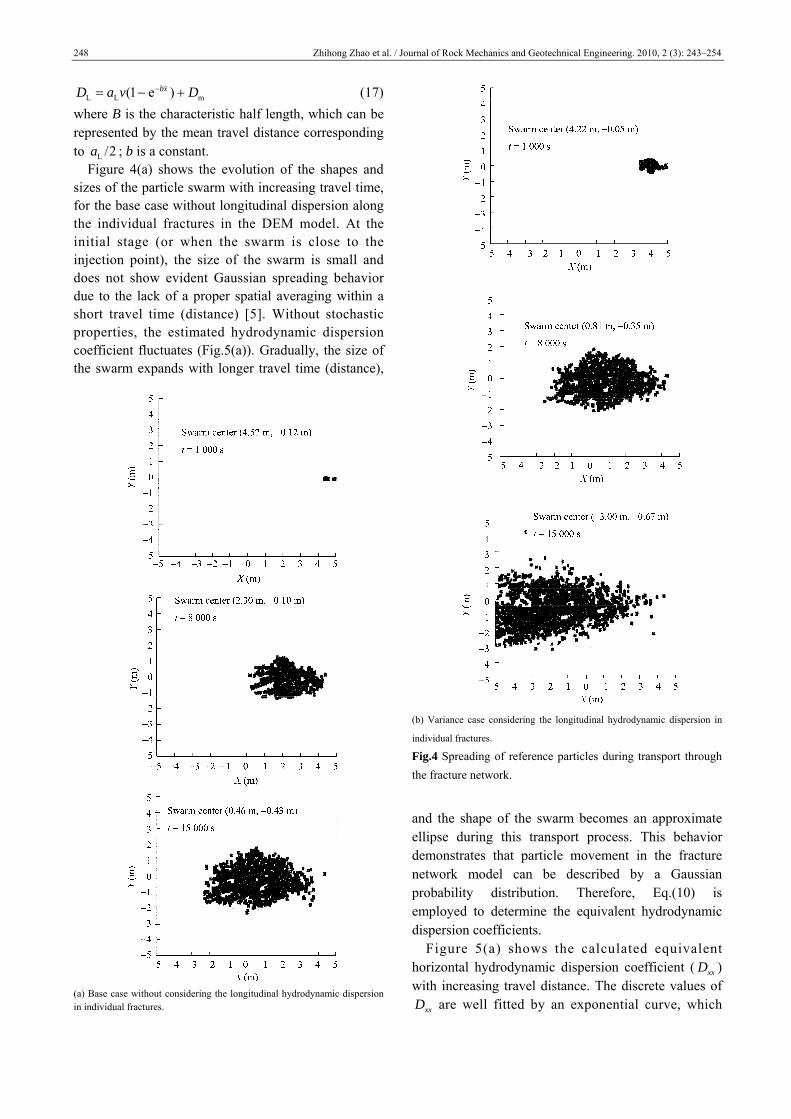
Since there are no available experimental results for flow and transport processes in fracture systems, the accuracy and ability of the proposed method are verified by comparison with the theoretical or empirical scale-dependent hydrodynamic dispersion models proposed in literatures, without longitudinal dispersion in single fractures. The commonly accepted and widely used scale-dependent hydrodynamic dispersion models are in asymptotic or exponential forms [18–20], given by

L L m[1 / ( )]D a v B B x D (16)

h =

5 1

01 5

20 M

Pa

v = 5 MPa

P1

= 2

.5×

105 P

a

P2

= 1

.5×

105 P

a

10 m

20 m


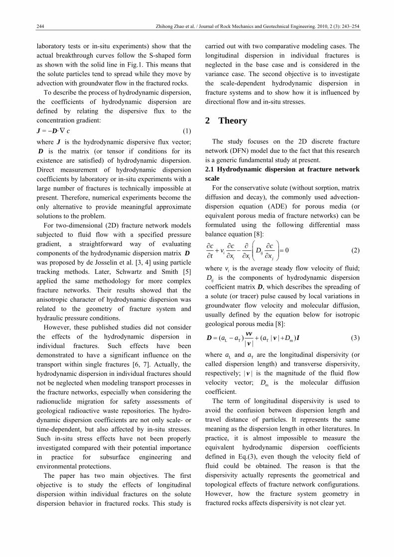
L L m(1 e )bxD a v D (17) where B is the characteristic half length, which can be represented by the mean travel distance corresponding to L /2a ; b is a constant.

Figure 4(a) shows the evolution of the shapes and sizes of the particle swarm with increasing travel time, for the base case without longitudinal dispersion along the individual fractures in the DEM model. At the initial stage (or when the swarm is close to the injection point), the size of the swarm is small and does not show evident Gaussian spreading behavior due to the lack of a proper spatial averaging within a short travel time (distance) [5]. Without stochastic properties, the estimated hydrodynamic dispersion coefficient fluctuates (Fig.5(a)). Gradually, the size of the swarm expands with longer travel time (distance),

(a) Base case without considering the longitudinal hydrodynamic dispersion in individual fractures.

(b) Variance case considering the longitudinal hydrodynamic dispersion in

individual fractures.

Fig.4 Spreading of reference particles during transport through

the fracture network.

and the shape of the swarm becomes an approximate ellipse during this transport process. This behavior demonstrates that particle movement in the fracture network model can be described by a Gaussian probability distribution. Therefore, Eq.(10) is employed to determine the equivalent hydrodynamic dispersion coefficients.

Figure 5(a) shows the calculated equivalent horizontal hydrodynamic dispersion coefficient ( xxD ) with increasing travel distance. The discrete values of

xxD are well fitted by an exponential curve, which


(a) Base case without considering the longitudinal hydrodynamic dispersion in individual fractures.

(b) Variance case considering the longitudinal hydrodynamic dispersion in individual fractures.

Fig.5 Horizontal hydrodynamic dispersion coefficient ( )xxD

with increasing travel distance.

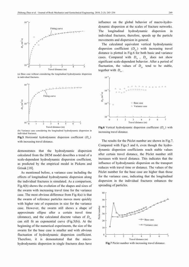
demonstrates that the hydrodynamic dispersion calculated from the DEM model describes a trend of a scale-dependent hydrodynamic dispersion coefficient, as predicted by the empirical model in Pickens and Grisak [18].

As mentioned before, a variance case including the effects of longitudinal hydrodynamic dispersion along the individual fractures is simulated. As a comparison, Fig.4(b) shows the evolution of the shapes and sizes of the swarm with increasing travel time for the variance case. The most obvious difference from Fig.4(a) is that the swarm of reference particles moves more quickly with higher rate of expansion in size for the variance case. However, the swarm still shows a shape of approximate ellipse after a certain travel time (distance), and the calculated discrete values of xxD can still fit an exponential curve (Fig.5(b)). At the beginning of the numerical experiments, the size of the swarm for the base case is smaller and with obvious fluctuation of hydrodynamic dispersion coefficient. Therefore, it is demonstrated that the micro-hydrodynamic dispersion in single fractures does have

influence on the global behavior of macro-hydro-dynamic dispersion at the scales of fracture networks. The longitudinal hydrodynamic dispersion in individual fractures, therefore, speeds up the particle movements and dispersion in general.

The calculated equivalent vertical hydrodynamic dispersion coefficient ( )yyD with increasing travel distance is plotted in Fig.6 for both basic and variance cases. Compared with xxD , yyD does not show significant scale-dependent behavior. After a period of fluctuation, the values of yyD tend to be stable, together with xxD .

Fig.6 Vertical hydrodynamic dispersion coefficient ( )yyD with

increasing travel distance.

The results for the Péclet number are shown in Fig.7. Compared with Figs.5 and 6, even though the hydro-dynamic dispersion coefficients reach stable values after certain travel distance, the Péclet number still increases with travel distance. This indicates that the influence of hydrodynamic dispersion on the transport reduces with travel time or distance. The values of the Péclet number for the base case are higher than those for the variance case, indicating that the longitudinal dispersion in the individual fractures enhances the spreading of particles.

Fig.7 Péclet number with increasing travel distance.

Travel distance (m) 0 1 2 3 4 5

106

105

104 D

xx (

m2 /s

)

Fitting curve

0 1 2 3 4 5 6 7

Travel distance (m)

104

105

106

Dxx

(m

2 /s)

Fitting curve

0 1 2 3 4 5 6 7

Base case Variance case

Travel distance (m)

Dyy

(m

2 /s)

107

106

105

104

Travel distance (m) 0 1 2 3 4 5 6 7

0

10

20

30

40

50

60

Péc

let n

umbe

r

Base case

Variance case


3.2 Influence of hydraulic conditions As mentioned before, the hydrodynamic dispersion

coefficients are dependent on the fluid velocity field, in addition to the geometry of the fracture system. In order to study the influence of directional flow on the anisotropy of the hydrodynamic dispersion coefficients, we rotate the fracture network in an interval of 30° (Fig.3(a)) anticlockwise and repeat the same numerical experiments using the hydraulic boundary conditions as shown in Fig.3(b). For each rotated model, we calculate the corresponding hydrodynamic dispersion coefficients, both along and perpendicular to the major flow direction. Note that this method is equivalent to rotating the direction of the specified hydraulic gradient.

The upper sub-figures in Figs.8(a) and (b) show the equivalent hydrodynamic dispersion coefficients changing with the rotated DFN models for the base case. With the changes in main flow direction, the values of longitudinal hydrodynamic dispersion coefficient ( xxD ) vary from 1.83×105 to 3.85×105 m2/s at t = 15 000 s. This indicates that the flow direction has a significant influence on the hydrodynamic dispersion in the fracture network model. To identify the contributions of the geometry of fracture network and flow velocity variations to the hydrodynamic dispersion coefficients, we plot the longitudinal dispersivity ( La ) and mean flow velocity ( Lv ) changing with rotated DFN models, as shown in Figs.8(c) and 8(d), respectively. The plots show that the molecular diffusion plays a minor role on the hydrodynamic dispersion, so the hydrodynamic dispersion coefficient is mainly dependent on the longitudinal dispersivity and the flow velocity (Eq.(5)). The smallest longitudinal dispersivity happens in the direction of 60°–240°, with the largest mean flow velocity in this direction. In general, if the flow direction is approximately parallel to the dip direction of fracture set, one has a larger flow velocity (or permeability) and a smaller longitudinal dispersivity, and vice versa.

The effects of directional flow on the equivalent hydrodynamic dispersion coefficients for the variance case are shown in Fig.8 (the lower sub-figures). One difference is that the values of equivalent hydro dynamic dispersion coefficients for variance case are larger than those for base case. At t =15 000 s, values of xxD vary from 4.26×105 to 7.45×105 m2/s. The geometrical influence on the longitudinal dispersivity is similar between two cases because of the similar shape in Fig.8(c).

(a) Dxx.

(b) Dyy.

Variance case t = 8 000 s

0

30

60 90

120

150

180

210

240270

300

330

0.0

1.0105

2.0105

3.0105

1.0105

2.0105

3.0105

Dyy

(m

2 /s)

t = 12 000 s t = 15 000 s

Dyy

(m

2 /s)

t = 8 000 s t = 12 000 s t = 15 000 s

Base case

0

30

6090

120

150

180

210

240270

300

330

3.0105

2.0105

1.0105

0.0

1.0105

2.0105

3.0105

0

30

60

90 120

150

180

210

240 270

300

330

1.0104

8.0105

6.0105

4.0105

2.0105

0.0

2.0105

4.0105

6.0105

8.0105

1.0104

Dxx

(m

2 /s)

t = 8 000 s t = 12 000 s t = 15 000 s

Base case

t = 8 000 s t = 12 000 s t = 15 000 s

0

30

60

90 120

150

180

210

240 270

300

330

1.0104

8.0105

6.0105

4.0105

2.0105

0.0

2.0105

4.0105

6.0105

8.0105

1.0104

Dxx

(m

2 /s)

Variance case


(c) Longitudinal dispersivity.

(d) Mean flow velocity.

Fig.8 Influence of directional flow on the hydrodynamic dispersion.

3.3 Influence of stress In order to study the influence of stress on the

hydrodynamic dispersion, an isotropic stress of 5 MPa is applied to compressing the DEM model firstly. Then the stress is increased at the left and right vertical boundaries with an interval of 5 MPa, till 20 MPa, to generate shear dilation (Fig.3(c)). The behaviors of fractures under stress can be found in Ref.[16–21]. The stress ratio K is defined as the ratio of horizontal/ vertical stress for sake of simple expression, which increases from 55 to 205. K = 00 represents an initial stress free state, under which the results are presented in Section 3.1. After a mechanical equilibrium state of

the DEM model under the stress boundary conditions is obtained, fluid flow through the deformed DEM model is simulated by applying the same hydraulic boundary condition as shown in Fig.3(b). Finally, the particle transport simulation is done based on the fluid flow velocity fields and deformed fracture network geometry data that are generated by the DEM model. Note that we only investigate the variance case considering longitudinal hydrodynamic dispersion in single fractures here, because its influence has been demonstrated in the previous sections.

Figure 9 shows a comparison of shapes and sizes of the particle swarms with increasing stress ratios at t = 60 000 s. Under the conditions of isotropic stress (K = 5:5) or a stress ratio of K = 10:5, the swarm of reference particles, showing a Gaussian behavior, moves much slowly, compared with the case under the

(a) K = 5:5.

(b) K = 10:5.

(c) K = 15:5.

270

240

Variance case

t = 8 000 s

0.00

0.05

0.10

0.15

0.20

0

30

6090

120

150

180

210

240270

300

330

0.05

0.10

0.15

0.20

t = 12 000 s t = 15 000 s

a L

1.0107

1.5107

0

30

6090

120

150

180

210

240270

300

330

0.0

5.0108

1.0107

1.5107

5.0108

Mea

n fl

ow v

eloc

ity (

m/s

)

Base case

t = 8 000 s

0.00

0.05

0.10

0.15

0.20

0

30

60

90 120

150

180

210

300

330

0.05

0.10

0.15

0.20

a L

t = 12 000 s t = 15 000 s


(d) K = 20:5.

Fig.9 Spreading of reference particles during transport through

the fracture network at t = 60 000 s.

stress-free condition (K = 0:0, Fig.4(b)), but retains the general shape of approximate ellipse during its movement. The reason is that all the fractures undergo normal closure under these stress conditions, which results in almost uniformly decreasing fracture apertures and flow rates (Fig.10(a)). For the same travel distance, it needs 5 times more than that under the condition of K = 0:0. Through a comparison of the magnitudes of longitudinal hydrodynamic dispersion coefficient at the same travel distance, we find that they are decreased by 5 times as well (Fig.11(a)). We can conclude that the decreasing hydrodynamic dispersion is included by the decreasing flow rates.

(a) K = 5:5.

(b) K = 20:5.

Fig.10 Flow rate distribution with stress applied (Thickness of the line represents the magnitude of flow rate. Each line represents the flow rate of 1×109 m3/s, and flow rates smaller than this value are not shown).

(a) Dxx.

(b) Dyy.

Fig.11 Hydrodynamic dispersion coefficients changing with increasing stress ratio for case considering longitudinal hydrodynamic dispersion in individual fractures.

This effect can also be demonstrated by the similar longitudinal dispersivity values of 1.2 and 1.3, respectively, before and after stress is applied. Therefore, for the fracture network model with approximately uniform apertures, fracture aperture plays a minor role in longitudinal dispersivity. For the scale-dependent hydrodynamic dispersion coefficients ( xxD and yyD ), they increased steadily before reaching a travel distance of 2 m, after that they leveled off to some asymptotic values (Fig.11). By fitting the discrete values of xxD using exponential curve, we find that the behavior of hydrodynamic dispersion can be still described by a scale-dependent hydrodynamic dispersion coefficient in an exponential form (Eq.(17)).

After K = 15:5, the shape of reference particle swarm becomes more irregular (Figs.9 (c) and (d)), induced by the influence of channeling of the fluid flow due to the shear dilations under higher stress ratios. The percentage of fractures with larger aperture than initial aperture of 30 μm increases (Fig.12). A large number of particles follow a few big channels,

0 1 2 3 4 5 6107

106

105

K = 0:0 K = 5:5 K = 10:5 K = 15:5 K = 20:5

Travel distance (m)

104

Dyy

(m

2 /s)

0 1 2 3 4 5 6106

105

104

K = 0:0 K = 5:5 K = 10:5 K = 15:5 K = 20:5

Travel distance (m)

103

Dxx

(m

2 /s)


Fig.12 Fracture aperture distribution with increasing stress ratio (For the initial case without stress applied (K = 0:0), the fracture aperture is a constant of 30 μm).

consisting of fractures with larger shear dilation (Fig.10(b)). The values of longitudinal hydrodynamic dispersion coefficient ( xxD ) increase drastically, and then decrease. The reason for the decreasing equivalent hydrodynamic dispersion is that a part of reference particles following the big channels exit the DFN models. Neretnieks [2] showed that channeling would make the equivalent hydrodynamic dispersion coefficients increase with the travel distance, which was in accord with our results. The values of yyD also increase with increasing travel distance (Fig.11(b)), compared to the nearly constant values of yyD under the stress-free state (K = 0:0).

Figure 13 shows that the Péclet number changes with travel distance under different stress ratios. When the isotropic stress is applied, the Péclet number increases compared with that at K = 0:0 because of the decreasing hydrodynamic dispersion coefficients. With continuously increasing stress ratio, the Péclet number decreases in contrast to the increasing hydrodynamic dispersion coefficient with increasing stress ratio. This is in line with the fact that low Péclet number corresponds to high hydrodynamic dispersion effect. To try to explain the stress influence on the hydrodynamic dispersion, we plotted the aperture distribution under different stress ratios, as shown in Fig.12. The peak of the aperture distribution shifts in the direction of small magnitude of aperture as stress ratio increases. A large number of fractures continue to close, and the portion of open fractures increases. The results show an obvious channeling effect with a few dominant flow paths and they are caused by stress conditions. This makes the stress effect on the hydrodynamic dispersion process in fracture network more significant.

Fig.13 Péclet number changing with increasing stress ratio for variance case.

4 Discussions and conclusions

A numerical procedure to determine the equivalent hydrodynamic dispersion coefficients and Péclet number of fractured rocks is presented with a random walk particle tracking method. Numerically calculated equivalent hydrodynamic dispersion coefficients can be represented by a function of travel distance in an exponential form for the tested fracture system with a constant initial aperture. The trend of the calculated hydrodynamic dispersion behavior agrees well with that of the usually accepted empirical models. The variance case shows that the longitudinal hydro-dynamic dispersion in individual fractures could have a significant influence on the macro-hydrodynamic dispersion of the full scale of fracture networks. It enhances the spreading of particles, and increases the values of the equivalent hydrodynamic dispersion coefficients. These results represent an enhancement to our understanding on the conceptual behavior of the transport of solute in fractured rocks.

The proposed method is used to study the influence of directional flow and stress on the behaviors of macro-hydrodynamic dispersion of fracture networks with stochastic geometrical properties, and some useful insights are obtained. Some important concluding remarks are presented below: (1) The scale- or time-dependent hydrodynamic dispersion coefficients can be described by an asymptotic or exponential function of travel distance (or time). (2) The anisotropy of fracture system determines different hydrodynamic dispersion coefficients under different flow directions. If the flow direction is approximately parallel to the dip direction of fracture sets, smaller hydrodynamic dispersion coefficients are generated. (3) Stress has a considerable effect on the fracture system configuration, flow field and macro-hydrodynamic dispersion. Smaller stress ratios significantly decrease the magnitudes of hydrodynamic dispersion coefficients,

5.01051.0105 2.0105 3.0105 4.0105 0.0

0.1

0.2

0.3

0.4

0.5

0.6

K = 5:5 K = 10:5 K = 15:5 K = 20:5

Fre

quen

cy

Aperture (m)

0 1 2 3 4 5 60

10

20

30

40

50

60 K = 0:0 K = 5:5 K = 10:5 K = 15:5 K = 20:5

Péc

let n

umbe

r

Travel distance (m)


but the relation between hydrodynamic dispersion coefficients and travel distance remains to be in an asymptotic or exponential form. The hydrodynamic dispersion coefficients do not reach a constant value as increasing travel distance under higher stress ratios, due to the influence of channeling phenomenon caused by shear dilations of the fractures. (4) The Péclet number increases with increasing travel distance, which means that the hydrodynamic dispersion contributes less to the transport of particles, compared with advection.

Although this paper provides some basic insights into understanding the behavior of hydrodynamic dispersion in fracture systems, some important issues are discussed below.

The 2D DFN model is used mainly for its simplicity. But the proposed methodology can be extended to a three-dimensional DFN model without major theoretical difficulties. The study assumes that the rock matrix is impermeable, and the fluid flow only happens in the fractures. This assumption is acceptable for the short time scale or relatively large flow velocity [2]. However, if the problem is considered at the time scale of performance/safety assessments, the above assumption may be questionable because the matrix diffusion probably becomes an important factor. The factor may significantly increase the solute residence time and change the distribution of reference particles. The effects of matrix diffusion on dispersion cannot be neglected under those cases, and a model including matrix diffusion is needed.

The DEM model setup requires a fracture system regularization, by which the isolated fractures and dead-ends are removed for mechanical and flow simulations. In this way, no stagnant water exists in the isolated fractures or dead-ends within the rock blocks. The influence of removing the isolated fractures and dead-ends may need to be investigated in the future to see if it has significant effects on the transport processes.

This study assumes a constant initial fracture aperture for the entire fracture network model for simplicity. The methodology proposed in this paper can be applied to studying the more realistic fracture networks with varying apertures, or correlated to fracture lengths. However, larger DFN models are expected to generate stable hydrodynamic dispersion coefficients, and more powerful computational ability is needed.

The fractures are idealized as a smooth parallel plate model, with the cubic law for fluid flow in them. This makes it impossible to properly reflect the effect of

roughness of fracture surfaces on the behaviors of microscopic or macro-hydrodynamic dispersion.

Acknowledgement

We would like to acknowledge the financial supports from Swedish Nuclear Fuel and Waste Management Co. (SKB) through the DECOVALEX-2011 project. References

[1] Bear J, Buchlin J M. Modeling and applications of transport phenomena in porous media. [S.l.]: Kluwer Academic Publishers, 1991.

[2] Neretnieks I. A note on fracture flow dispersion mechanism in the ground. Water Resources Research, 1983, 19 (2): 364–370.

[3] de Josselin de Jong G, Way S C. Dispersion in fissured rock. Socorro, New Mexico: Institute of Mining and Technology, 1972.

[4] Way S C, McKee C R. Restoration of in-situ coal gasification sites from naturally occurring flow and dispersion. In Situ, 1981, 5 (2): 77–101.

[5] Schwartz F W, Smith L. A continuum approach for modeling mass transport in fractured media. Water Resources Research, 1988, 24 (8): 1 360–1 372.

[6] Bodin J, Delay F, de Marsily G. Solute transport in a single fracture with negligible matrix permeability: 1. fundamental mechanisms. Hydrogeology Journal, 2003, 11 (4): 418–433.

[7] Bodin J, Delay F, de Marsily G. Solute transport in a single fracture with negligible matrix permeability: 2. mathematical formalism. Hydrogeology Journal, 2003, 11 (4): 434–454.

[8] Salamon P, Fernàndez-Garcia D, Gómez-Hernàndez J. A review and numerical assessment of the random walk particle tracking method. Journal of Contaminant Hydrology, 2006, 87 (3/4): 277–305.

[9] Rasmuson A, Neretnieks I. Migration of radionuclides in fissured rock: the influence of micropore diffusion and longitudinal dispersion. Journal of Geophysical Research, 1981, 86 (B5): 3 749–3 758.

[10] Gelhar L W. Stochastic subsurface hydrology. New York: Prentice Hall, 1993.

[11] Ogata A, Banks R B. A solution of the differential equation of longitudinal dispersion in porous media. [S. l.]: U. S. Geological Survey, 1961: 1–7.

[12] Yamashita R, Kimura H. Particle-tracking technique for nuclide decay chain transport in fractured porous media. Journal of Nuclear Science and Technology, 1990, 27 (11): 1 041–1 049.

[13] Grubert D. Effective dispersivities for a two-dimensional periodic fracture network by a continuous time random walk analysis of single-intersection simulations. Water Resources Research, 2001, 37 (1): 41–49.

[14] Lee C, Lee C, Lin B. The estimation of dispersion behavior in discrete fractured networks of andesite in Lan-Yu Island, Taiwan. Environmental Geology, 2007, 52 (7): 1 297–1 306.

[15] Itasca Consulting Group Inc.. UDEC user’s guide. Minneapolis: Itasca Consulting Group Inc., 2004.

[16] Min K B, Rutqvist J, Tsang C F, et al. Stress-dependent permeability of fractured rock masses: a numerical study. International Journal of Rock Mechanics and Mining Sciences, 2004, 41 (7): 1 191–1 210.

[17] Baghbanan A, Jing L. Stress effects on permeability in fractured rock masses with correlated fracture length and aperture. International Journal of Rock Mechanics and Mining Sciences, 2008, 45 (8): 1 320–1 334.

[18] Pickens J F, Grisak G E. Modeling of scale-dependent dispersion in hydrogeologic systems. Water Resources Research, 1981, 17 (6): 1 701–1 711.

[19] Yates S R. An analytical solution for one-dimensional transport in porous media with an exponential dispersion function. Water Resources Research, 1992, 28 (8): 2 149–2 154.

[20] Huang K, van Genuchten M T, Zhang R. Exact solutions for one-dimensional transport with asymptotic scale-dependent dispersion. Applied Mathematical Modelling, 1996, 20 (4): 298–308.

[21] Zhao Z, Jing L, Neretnieks I, et al. Numerical modeling of stress effects on solute transport in fractured rocks. Computers and Geotechnics, 2010 (to be published).

Documents

Evaluation of hydrodynamic dispersion parameters in ... · Evaluation of hydrodynamic dispersion parameters in fractured rocks ... equivalent porous media of fracture networks)