Evaluation of IEEE802.15.4g for Environmental Observations

HAL Id: hal-01968648https://hal.inria.fr/hal-01968648

Submitted on 2 Jan 2019

HAL is a multi-disciplinary open accessarchive for the deposit and dissemination of sci-entific research documents, whether they are pub-lished or not. The documents may come fromteaching and research institutions in France orabroad, or from public or private research centers.

L’archive ouverte pluridisciplinaire HAL, estdestinée au dépôt et à la diffusion de documentsscientifiques de niveau recherche, publiés ou non,émanant des établissements d’enseignement et derecherche français ou étrangers, des laboratoirespublics ou privés.

Evaluation of IEEE802.15.4g for EnvironmentalObservations

Jonathan Munoz, Tengfei Chang, Xavier Vilajosana, Thomas Watteyne

To cite this version:Jonathan Munoz, Tengfei Chang, Xavier Vilajosana, Thomas Watteyne. Evaluation of IEEE802.15.4gfor Environmental Observations. Sensors, MDPI, 2018. �hal-01968648�

https://hal.inria.fr/hal-01968648

https://hal.archives-ouvertes.fr

Article

Evaluation of IEEE802.15.4g for EnvironmentalObservationsJonathan Muñoz1,∗, Tengfei Chang1, Xavier Vilajosana2, Thomas Watteyne1

1 Inria, EVA team, Paris, France.2 Universitat Oberta de Catalunya, Barcelona, Spain.* Correspondence: [email protected]

Version October 8, 2018 submitted to Sensors; Typeset by LATEX using class file mdpi.cls

Abstract: IEEE802.15.4g is a low-power wireless standard initially designed for Smart Utility1

Networks, i.e. for connecting smart meters. IEEE802.15.4g operates at sub-GHz frequencies to offer2

2–3× longer communication range compared to its 2.4 GHz counterpart. Although the standard3

offers 3 PHYs (FSK, OFDM and O-QPSK) with numerous configurations, 2-FSK at 50 kbps is the4

mandatory and most prevalent radio setting used. This article looks at whether IEEE802.15.4g can5

be used to provide connectivity for outdoor deployments. We conduct range measurements using6

the totality of the standard (all modulations with all further parametrization) in the 863 – 870 MHz7

band, within four scenarios which we believe cover most low-power wireless outdoor applications:8

line of sight, smart agriculture, urban canyon, and smart metering. We show that there are radio9

settings that outperform the “2-FSK at 50 kbps” base setting in terms of range, throughput and10

reliability. Results show that highly reliable communications with data rates up to 800 kbps can11

be achieved in urban environments at 540 m between nodes, and the longest useful radio link is12

obtained at 779 m. We discuss how IEEE802.15.4g can be used for outdoor operation, and reduce13

the number of repeater nodes that need to be placed compared to a 2.4 GHz solution.14

Keywords: Wireless Sensor Networks; Environmental Observations; IEEE802.15.4g; sub-GHz;15

Range Measurements.16

1. Introduction17

Low-power wireless mesh (sensor) networks drastically decrease the cost of implementing18

monitoring/control systems, enabling a wide range of applications in the industrial, environmental19

and urban context. Wireless mesh networks are used over a wide spectrum of environmental20

observation applications, including smart agriculture [1], fire monitoring [2], seismic activity21

logging [3], and snow-pack monitoring [4].22

In these applications and many others, the IEEE802.15.4 standard is often used to provide23

connectivity between sensor nodes. Most deployments use the 2.4 GHz version of this standard,24

with O-QPSK modulation, 16 frequencies, and a maximum frame length of 127 B [5]. When sensors25

need to cover a large area, repeater nodes often need to be added to ensure that the deployment is26

dense enough. Malek et al. [4] for example reported the need of installing three times more repeaters27

than sensor nodes, increasing the cost and time of deployment. With IEEE802.15.4 at 2.4 GHz, radio28

links are typically 100 m, sometimes up to 300 m, but with a range that drastically decreases when29

obstacles (such as trees) are between the nodes.30

Analysis of sub-GHz based communications for environmental observations have also been31

carried out. Kjeldsen et al. [6] and Zhou et al. [7] study the radio waves propagation in sub-terrain32

environments such as mines and sewers. Both studies conclude that in those environments the radio33

waves propagate as inside a waveguide. The smaller the cross-section area of the structure, more34

attenuation happen for lower frequencies (sub-GHz) than for higher frequencies (2.4 and 5.8 GHz).35

Submitted to Sensors, pages 1 – 39 www.mdpi.com/journal/sensors

http://www.mdpi.com

http://www.mdpi.com/journal/sensors

Version October 8, 2018 submitted to Sensors 2 of 39

Thelen et al. [8] present an extensive set of measurements taken in a potato field of 154 m36

× 105 m in order to study how the environmental conditions affects the performance of the radio37

communications. For their experiment they used 13 Mica2Dot nodes with a Chipcon CC1000 radio38

chip in the 433 MHz band, working with a FSK modulation, 19.2 kbps and +10 dBm TX power. Nodes39

are placed on the ground and the antennae are at a height of 11 cm. Meanwhile one node transmitted,40

the rest of the nodes listen and stored the amount of received packets and their Received Strength41

Signal Indicator (RSSI) value. It is perceived that radio waves propagated better with conditions42

of high humidity, e.g., during rain and at nights. They concluded that for reliable communication43

(RSSI ≥ -90 dBm), nodes need to be separated for at most 10 m for during blooming (potato plants44

grow up to 1 m approximately) and 23 m when the crop is on its return.45

Hartung et al. [2] described FireWxNet: an hybrid wireless system to monitor weather46

conditions. This system allow the fire fighters to measure fire and weather conditions in order to47

predict fire behavior and reduced the damages caused by these events. Two sensor networks was48

deployed in the Bitterroot National Forest. The nodes used are based on the Mica2 platform featuring49

a Chipcon CC1000 radio operating at 900 MHz, with a maximum TX power of +10 dBm. Nodes were50

mounted on a tripod at 1.5 m from the ground and are located on the surface of the Hell’s Half Acre51

and Kit Carson mountains, at different heights. Stable radio links up to 400 m are formed.52

Lazarescu [9] described the design considerations of a low cost WSN for wildfire monitoring. It53

is used a 50 node deployment using the 433 MHz frequency band, connecting to a gateway embedded54

inside a wooden birdhouse with solar panels on the top. The antenna of the gateway was left inside55

the box. This choice reduced drastically the quality of the radio links between gateway and sensor56

nodes, allowing communication ranges only up to 70 m.57

Cerpa et al. [10] presented SCALE, a measurement visualization tool that allow the collection58

of packet delivery statistics and can help to engineers to determine data capacity and latency of the59

system. They used the same micro-controller with two types of radios, a RFM TR1000 and a Chipcon60

CC1000. The former working at 916 MHz, 13.3 kbps with a Amplitude Shift Keying (ASK) modulation61

and the latter at 433 MHz, 19.2 kbps and FSK. They show that radio links of 50 m with PDR over 60 %62

are achieved in outdoor environments, with a 0 dBm TX power with the TR1000 radio. Due to the lack63

of more hardware, they could not test over longer distances. They conclude that there is no evident64

correlation between PDR and distance for more than 50 % communication range.65

The IEEE802.15.4 standard continuously evolves. In 2012, the “g” amendment to the66

standard [11] added a new physical layer, with three modulations (FSK, OFDM and O-QPSK), and a67

maximum frame size of 2047 B. Most importantly, IEEE802.15.4g is designed to operate in sub-GHz68

bands (such as 863–870 MHz in Europe, 902–928 MHz band in the US), increasing communication69

range for the output power, when compared to 2.4 GHz. Nonetheless, it can also be used at 2.4 GHz.70

The Wi-SUN industrial alliance1 has adopted this amendment, specifically the 2–FSK 50 kbps71

option. This is one of the most frequently implemented options in smart metering applications 2. As72

a result, most “IEEE802.15.4g compliant” chips only implement that option.73

In opposition to the 2.4 GHz band, license-free sub-GHz bands are at different frequencies in74

different countries, and are subjected to regional regulations. This means that devices compliant in75

one region may not be suitable to be deployed in another. One example is the European regulation,76

that imposes a duty cycle of < 0.1%, or 3.6 s of transmit time over one hour while The United States77

imposes a duty cycle of < 2%.78

This study explores the entire “g” amendment, i.e. all three modulations techniques with their79

further parametrization. The result is that IEEE802.15.4g contains 31 different radio settings, with80

1 www.wi-sun.org2 other sub-GHz solutions are popular, such as wireless M-Bus, LoRa, Sigfox.


data rates ranging from 6.25 kbps to 800 kbps, and channel bandwidth from 200 kHz to 1.2 MHz in81

the European sub-GHz band.82

Some studies of IEEE802.15.4g already exist. Sum et al. [12] evaluate the performance of83

a WPAN when using the IEEE802.15.4/4e/4g for smart utility networks through simulations.84

Dias et al. [13] deploy a WSN in office/canteen/warehouse buildings in a smart grid application, and85

evaluate the performance of a single radio setting (O-QPSK, 250 kbps, 2 MHz channel bandwidth).86

Mochizuki et al. [14] propose an enhancement to a conventional Wi-SUN system by increasing the87

transmission power of the downlink communication, and using a 2-FSK 100 kbps setting for their88

system tested in the city of Kyoto.89

Sum et al. [15] study the communication and interference range for deployments for90

IEEE802.15.4g Smart Utility Network (SUN) devices in low and high dense environments (from91

10 up to 2500 devices per square kilometer). Based on realistic channel models and assuming92

FSK modulation with -90 dBm sensitivity, they conclude that the communication range in urban93

environments (PER ≤ 1%) for SUN devices is 33 m, 65 m and 104 m when using 2.4 GHz, 915 MHz94

and 460 MHz frequency bands respectively.95

Bragg et al. [16] deployed six sensor nodes and two dedicated routing nodes in the Cairngorm96

Mountains in Scotland. The Zolertia Z1 sensor mote with a CC1120 radiochip was the hardware97

choice for the nodes. These were separated into two clusters covering one kilometer square area. The98

border router was located 3.5 km away of the closest router. The data rate was set to 50 kbps. The99

deployment showed that the radios can provide a single hop communication over that distance. By100

using a Line of Sight propagation model for a CC2420 radio (implementing O-QPSK PHY, 250 kbps101

at 2.4 GHz), they determined that for a solution using this radio would need at least 25 routing nodes.102

Through simulations and outdoor experimentation, Kojima et al. [17] investigate the feasibility of103

employing the Gaussian FSK PHY under multi-path conditions in a suburban area. With transmitter104

and receiver tunned at 413 MHz, with a BPSK modulation and a TX power of +10 dBm, the radio105

signal is received with a power level of -60 dBm. Results show that for a frame length of 1500 B,106

PER ≤ 10 % and considering a receiver sensitivity of -100 dBm, the coverage area of the radio link is107

few hundred meters.108

All these IEEE802.15.4g studies and experiments have something in common: they only consider109

a single radio setting.110

What is missing is a comparative performance evaluation of all possible radio settings of111

IEEE802.15.4g, with a particular focus on communication range, performance and limits for different112

scenarios. Through experimentation, we test all IEEE802.15.4g radio settings in different scenarios113

where a wide range of applications can take place.114

The contribution of this article is three-fold:115

1. We define a system to carry out range testing of different radio settings with automatic116

out-of-band synchronization and minimum human intervention.117

2. We determine the best radio setting(s) to be used in the scenarios covered in this study, taking118

into account Packet Delivery Ratio (PDR), “goodput” (nominal data rate times the PDR), electric119

charge consumption and communication range.120

3. We provide an executive summary of the regulation on sub-GHz band usage in Europe, the US121

and Japan.122

The remainder of the article is organized as follows. Section 2 details the materials used for the123

experiments, explains the main sub-GHz regulation, and describes the characteristics of the scenarios124

and PHYs tested. Section 3 shows the PDR for each scenario at different communication ranges.125

Section 4 determines the most fitting PHYs per scenario according to PDR value, throughput and126

power consumption. Section 5 concludes this article by presenting future work.127

2. Materials and Methods128

We use the networking term “PHY” (physical layer) interchangeably with “radio setting”.129


Section 2.1 provides an overview of the PHYs being tested, Section 2.2 gives the main130

characteristics of the regulations of Europe, the United States and Japan when using sub-GHz bands.131

Section 2.3 and Section 2.4 describe the hardware and software used in these range test experiments,132

respectively. Section 2.5 details the scenarios where the nodes were deployed.133

2.1. IEEE802.15.4g PHYs134

The “g” amendment of the IEEE802.15.4 standard has been specifically designed to target SUN135

applications. Its maximum packet size is 2047 B, enough to carry a complete IP packet in one136

frame without the need of implementing link-layer fragmentation. A longer communication range137

is needed by SUN applications, therefore the standard makes a more extensive use of the sub-GHz138

frequencies than the previous version of 2006, using O-QPSK.139

In sub-GHz bands, radio signals can cover longer distances with the same transmission power,140

compared to 2.4 GHz.141

In Europe, two of the most popular unlicensed ISM sub-GHz frequency bands for Non-Specific142

Short Range Devices are 433.05–434.79 MHz and 863–870 MHz [18,19]. For this study, we use the143

latter because the frequency band is wider (7 MHz vs. 1.74 MHz), allowing more communication144

channels. This band also provides a good trade-off between range and antenna dimension3.145

The IEEE802.15.4g includes three modulations:146

• Frequency Shift Keying (FSK). In transmission, it delivers good power efficiency thanks to the147

constant envelope of the signal. It may implement a Gaussian filter or be unfiltered. It uses148

convolutional coding as Forward Error Correction (FEC). This technique uses redundancy of149

information and gives the possibility to the receiver to correct errors by itself, without having150

to request a retransmission of the information. The price to pay is the reduced effective data151

rate, since more bits are needed to encode the same information. A FEC rate of 1/2 means152

that for 1 bit of information, 2 bits are transmitted. Data Whitening and interleaving are also153

optional. Data rates vary from 5 kbps to 400 kbps. SUN FSK devices are simple and do not154

require complex circuitry consuming high processing power, resulting in a less power-hungry155

technology. This PHY targets low data rates and high energy efficiency applications, e.g. smart156

metering. Most electric meters in the US use this PHY.157

• Orthogonal Frequency Division Multiplexing (OFDM): This PHY is designed to provide high158

data rate communication in challenging environments presenting multi-path fading conditions,159

such as urbanized areas or indoor scenarios. Here, the transmitted signals bounce off obstacles,160

taking different paths and some of them arriving to the receiver at slightly different times (with161

a different phase). As a result, the overall received signal is the complex sum of those reflections,162

which can constructively or destructively (self-)interfere. Multi-path fading is also dependent163

on the frequency used, i.e. it affects different frequencies in different ways. In order to cope with164

this, OFDM spreads the information to be transmitted over multiple sub-carriers occupying165

different frequencies. Each sub-carrier is modulated according to a Modulation and Coding166

Scheme (MCS) value, and it can be BPSK, QPSK and 16-QAM. If part of the data is lost, it can be167

recovered using FEC techniques and frequency repetition (2 or more sub-carriers transporting168

the same information). OFDM devices require a more complex circuitry with higher power169

consumption in order to carry out sophisticated signal processing functions such as creating or170

demodulating OFDM symbols. This technology has been widely applied in high-end systems171

such as cellular networks; its use in low power devices is new. Data rates vary from 50 kbps up172

to 800 kbps. Typical applications are security and surveillance systems, where high data rates173

are required.174

3 The recommended size of an antenna depends of the wavelength – λ – of the signal. For dipole antennas, using length λ/2is common. At 433 MHz, this translates top a 35 cm antenna, compared to a 17 cm at 863–870 MHz.


Table 1. Radio settings using FSK modulation. The values of these parameters are defined in thestandard [20]. Data rate values consider the amount of bits per second leaving the radio. In the casewhere FEC is used, 1 bit of information is encoded in 2 bits leaving the radio, therefore the informationrate reduces to half. Channel spacing is the separation between the center of two adjacent channels.The “Alias” column provides an identifier to each group of parameters.

PHY FEC Data rate Ch. spacing Alias1/2 rate

2-FSK No 50 kbps 200 kHz 2FSK-502-FSK No 100 kbps 400 kHz 2FSK-1004-FSK No 200 kbps 400 kHz 4FSK-2002-FSK Yes 50 kbps 200 kHz 2FSK-FEC-502-FSK Yes 100 kbps 400 kHz 2FSK-FEC-1004-FSK Yes 200 kbps 400 kHz 4FSK-FEC-200

• Offset Quadrature Phase Shift Keying (O-QPSK). It uses Direct Sequence Spread Spectrum175

(DSSS) or Multiplexed Direct Sequence Spread Spectrum (MDSSS), with data rates from 6 kbps176

up to 500 kbps. It shares some characteristics with IEEE802.15.4-2006, making multi-mode177

systems easier to design and more cost-effective [? ].178

These PHYs accept further parametrization, either by modifying the data rate (more information179

per symbol transmitted or more symbols per unit of time) and/or channel bandwidth. In this study,180

each PHY with a specific set of parameters is defined as radio setting and identified by an “alias”. In181

the 863–870 MHz frequency band, a total of 31 radio settings have been tested.182

Table 1 describes the radio settings for all the combinations of parameters using FSK and183

provides an “alias” to each of them. Tables 2 and 3 provide the same information for OFDM and184

O-QPSK, respectively. Only for the FSK radio settings implementing 12 rate FEC, the actual data rate185

is halved, since every two bits sent by the radio correspond to 1 bit of information. For the rest of the186

radio settings, the data rates stated in Tables 1, 2 and 3 are the data rates of the actual information187

leaving the radio.188

Table 2. Radio settings using OFDM modulation. The values of these parameters are defined inthe standard [20]. Channel spacing is the separation between the centers of two adjacent channels.OFDM channels group a number of sub-carriers, option 1 being the widest one (the most number ofsub-carriers), option 4 the narrowest (the least number of sub-carriers). The data rate depend on thecombination of the MCS (Modulation and Coding Scheme) value and the OFDM option. Frequencyrepetition identifies the number of sub-carriers encoding the same information. The “Alias” of eachradio setting is used to identify each set of parameter, e.g., OFDM1-400 identifies the PHY usingOFDM option 1 and MCS2.

Parameter OFDM Opt. 1 OFDM Opt. 2 OFDM Opt. 3 OFDM Opt. 4

Channel spacing (kHz) 1200 kHz 800 kHz 400 kHz 200 kHzNumber of sub-carriers 104 52 26 14

MCS0 (kbps) - 4x freq. rep. 100 kbps 50 kbps - -MCS1 (kbps) - 2x freq. rep. 200 kbps 100 kbps 50 kbps -MCS2 (kbps) - 2x freq. rep. 400 kbps 200 kbps 100 kbps 50 kbpsMCS3 (kbps) - 2x freq. rep. 800 kbps 400 kbps 200 kbps 100 kbpsMCS4 (kbps) - No freq. rep. - 600 kbps 300 kbps 150 kbpsMCS5 (kbps) - No freq. rep. - 800 kbps 400 kbps 200 kbpsMCS6 (kbps) - No freq. rep. - - 600 kbps 300 kbps

Alias OFDM1-<datarate> OFDM2-<datarate> OFDM3-<datarate> OFDM4-<datarate>


Table 3. Radio settings using O-QPSK modulation. The values of these parameters are defined in thestandard [20]. The rate mode defines the resulting data rate. The radio signal is composed by chips;in the 868 MHz frequency band, the standard uses a fixed 100 kchip/s. The spreading mode definesthe amount of chips needed to encode a bit of information.

Rate mode Chip rate Data rate Aliaskchip/s kbps

0 100 6.25 kbps OQPSK-6.251 100 12.5 kbps OQPSK-12.52 100 25 kbps OQPSK-253 100 50 kbps OQPSK-50

Using sub-GHz bands has two main drawbacks. First, license-free sub-GHz bands are not at the189

same frequency in all countries – unlike the 2.4 GHz ISM band – and each country/region makes its190

own selection of frequency to be assigned to unlicensed users:191

• In Europe, 863–870 MHz, with upcoming availabilities in the 870–876 MHz (early stages).192

• In the United States, 902–928 MHz.193

• In Japan, 922.4–928 MHz.194

Second, each country/region imposes (different) regulations to these sub-GHz bands. This195

significantly reduces the throughput of these networks, and products for one country may not satisfy196

the regaulations of another.197

2.2. Regional regulations198

Duty cycle, maximum bandwidth per communication channel, maximum dwell time and199

maximum transmission power are some of the parameters each region/country regulates. This200

section summarizes the regulations in Europe, the United States and Japan.201

2.2.1. Europe202

The European Telecommunication Standards Institute (ETSI) and the Electronic203

Communications Committee (part of the European Conference of Postal and Telecommunications204

Administrations, CEPT) define the set of recommendations and standards [18,21] for Short Range205

Devices operating in the 25–1000 MHz frequency band.206

Considering that the CEPT includes 48 European countries (national level) and ETSI has more207

than 800 members (regulatory bodies, governments, companies, universities, research bodies) from208

66 countries and five continents, their normative and regulations are complex, as consensus within209

the parties have to be made. In addition, some countries may differ on the designated bands or210

impose certain conditions on uses of specific bands.211

The normative for EU wide harmonized National Radio Interfaces cuts the 863–870 MHz band212

into sub-bands, as detailed in Table 4. Table 5 shows conformance to any National Radio Interface, in213

the case of using the entire 7 MHz band.214

The duty cycle restriction of 0.1% in some of the sub-bands could be eased and taken up to215

2.8% if polite spectrum access is applied to the transmitters. Polite spectrum access refers to Listen216

Before Talk (LBT) and Adaptability Frequency Agility (AFA). Prior to transmission, a “polite” device217

performs Clear Channel Assessment (CCA) to check its availability. If the channel is free, the device218

continues its transmission. If it is not, the device should not retry its transmission until a random time219

has passed. Optionally, the device can change the intended transmitting frequency and listens again220

before starts the transmission.221

The timing parameters of polite spectrum access are:222

• Minimum CCA time: 160 µs223


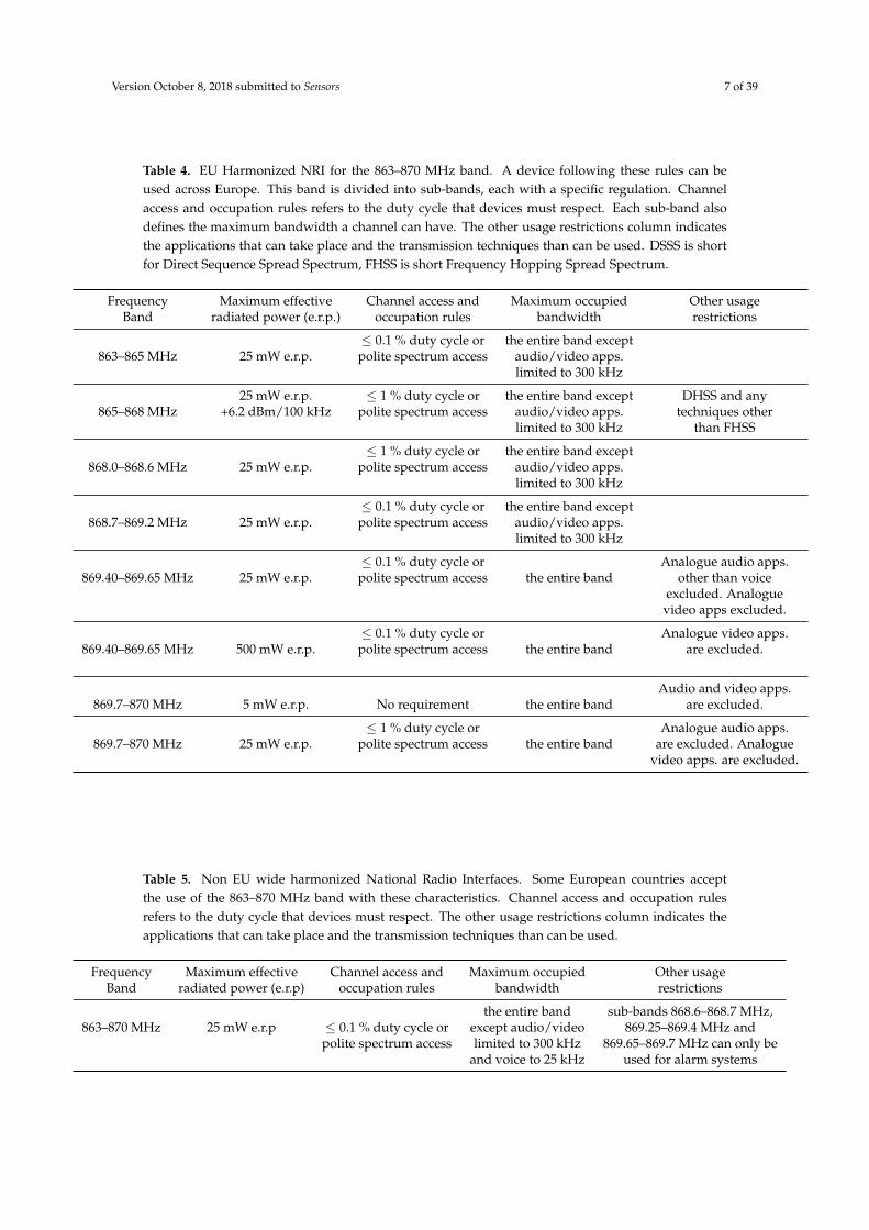
Table 4. EU Harmonized NRI for the 863–870 MHz band. A device following these rules can beused across Europe. This band is divided into sub-bands, each with a specific regulation. Channelaccess and occupation rules refers to the duty cycle that devices must respect. Each sub-band alsodefines the maximum bandwidth a channel can have. The other usage restrictions column indicatesthe applications that can take place and the transmission techniques than can be used. DSSS is shortfor Direct Sequence Spread Spectrum, FHSS is short Frequency Hopping Spread Spectrum.

Frequency Maximum effective Channel access and Maximum occupied Other usageBand radiated power (e.r.p.) occupation rules bandwidth restrictions

≤ 0.1 % duty cycle or the entire band except863–865 MHz 25 mW e.r.p. polite spectrum access audio/video apps.

limited to 300 kHz

25 mW e.r.p. ≤ 1 % duty cycle or the entire band except DHSS and any865–868 MHz +6.2 dBm/100 kHz polite spectrum access audio/video apps. techniques other

limited to 300 kHz than FHSS

≤ 1 % duty cycle or the entire band except868.0–868.6 MHz 25 mW e.r.p. polite spectrum access audio/video apps.

limited to 300 kHz

≤ 0.1 % duty cycle or the entire band except868.7–869.2 MHz 25 mW e.r.p. polite spectrum access audio/video apps.

limited to 300 kHz

≤ 0.1 % duty cycle or Analogue audio apps.869.40–869.65 MHz 25 mW e.r.p. polite spectrum access the entire band other than voice

excluded. Analoguevideo apps excluded.

≤ 0.1 % duty cycle or Analogue video apps.869.40–869.65 MHz 500 mW e.r.p. polite spectrum access the entire band are excluded.

Audio and video apps.869.7–870 MHz 5 mW e.r.p. No requirement the entire band are excluded.

≤ 1 % duty cycle or Analogue audio apps.869.7–870 MHz 25 mW e.r.p. polite spectrum access the entire band are excluded. Analogue

video apps. are excluded.

Table 5. Non EU wide harmonized National Radio Interfaces. Some European countries acceptthe use of the 863–870 MHz band with these characteristics. Channel access and occupation rulesrefers to the duty cycle that devices must respect. The other usage restrictions column indicates theapplications that can take place and the transmission techniques than can be used.

Frequency Maximum effective Channel access and Maximum occupied Other usageBand radiated power (e.r.p) occupation rules bandwidth restrictions

the entire band sub-bands 868.6–868.7 MHz,863–870 MHz 25 mW e.r.p ≤ 0.1 % duty cycle or except audio/video 869.25–869.4 MHz and

polite spectrum access limited to 300 kHz 869.65–869.7 MHz can only beand voice to 25 kHz used for alarm systems


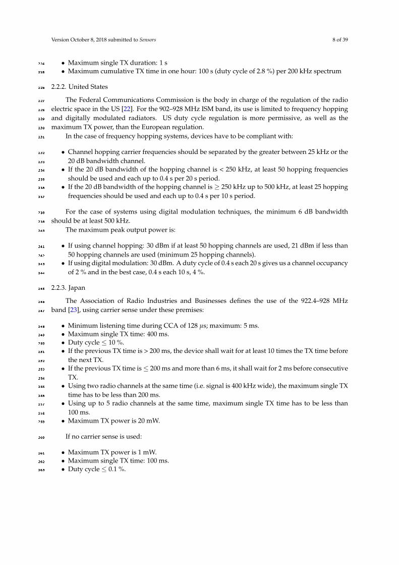
• Maximum single TX duration: 1 s224

• Maximum cumulative TX time in one hour: 100 s (duty cycle of 2.8 %) per 200 kHz spectrum225

2.2.2. United States226

The Federal Communications Commission is the body in charge of the regulation of the radio227

electric space in the US [22]. For the 902–928 MHz ISM band, its use is limited to frequency hopping228

and digitally modulated radiators. US duty cycle regulation is more permissive, as well as the229

maximum TX power, than the European regulation.230

In the case of frequency hopping systems, devices have to be compliant with:231

• Channel hopping carrier frequencies should be separated by the greater between 25 kHz or the232

20 dB bandwidth channel.233

• If the 20 dB bandwidth of the hopping channel is < 250 kHz, at least 50 hopping frequencies234

should be used and each up to 0.4 s per 20 s period.235

• If the 20 dB bandwidth of the hopping channel is ≥ 250 kHz up to 500 kHz, at least 25 hopping236

frequencies should be used and each up to 0.4 s per 10 s period.237

For the case of systems using digital modulation techniques, the minimum 6 dB bandwidth238

should be at least 500 kHz.239

The maximum peak output power is:240

• If using channel hopping: 30 dBm if at least 50 hopping channels are used, 21 dBm if less than241

50 hopping channels are used (minimum 25 hopping channels).242

• If using digital modulation: 30 dBm. A duty cycle of 0.4 s each 20 s gives us a channel occupancy243

of 2 % and in the best case, 0.4 s each 10 s, 4 %.244

2.2.3. Japan245

The Association of Radio Industries and Businesses defines the use of the 922.4–928 MHz246

band [23], using carrier sense under these premises:247

• Minimum listening time during CCA of 128 µs; maximum: 5 ms.248

• Maximum single TX time: 400 ms.249

• Duty cycle ≤ 10 %.250

• If the previous TX time is > 200 ms, the device shall wait for at least 10 times the TX time before251

the next TX.252

• If the previous TX time is ≤ 200 ms and more than 6 ms, it shall wait for 2 ms before consecutive253

TX.254

• Using two radio channels at the same time (i.e. signal is 400 kHz wide), the maximum single TX255

time has to be less than 200 ms.256

• Using up to 5 radio channels at the same time, maximum single TX time has to be less than257

100 ms.258

• Maximum TX power is 20 mW.259

If no carrier sense is used:260

• Maximum TX power is 1 mW.261

• Maximum single TX time: 100 ms.262

• Duty cycle ≤ 0.1 %.263


Figure 1. Node used in the range test measurement campaign.

2.3. Hardware264

This section describes the hardware used in the range measurement campaign. We used 4 nodes,265

1 configured as a TX (transmitter) and 3 others as RX (receiver). Each node is mounted on a 1.8 m266

PVC tube. From Watteyne et al [1] and Malek et al [4], we see their choice of putting their sensors at267

a height of 4 m on top of fixed wooden poles, reducing the impact the ground poses as an obstacle268

to the radio links. In our case, 1.8 m tubes reach the same height at which smart meters are located269

in a house. Therefore, the impact of the ground being an obstacle (e.g., Fresnel Zone obstruction) is a270

condition nodes have to cope with.271

2.3.1. Node272

A node consists of a Raspberry Pi 3 (rPi) model, an ATREB215-XPRO-A radio board evaluation273

kit, a 2 dBi omni-directional antenna, a GPS module and a push button; all housed in a plastic box. The274

rPi controls the radio board through a SPI bus. The electronic devices are powered by a 22,000 mAh275

battery bank. Fig. 1 shows a node.276

ATREB215-XPRO-A: This radio board features an AT86RF215 radio chip implementing both the277

IEEE802.15.4-2006 and the IEEE802.15.4g standards. It contains two transceivers, one for sub-GHz278

frequencies and the other for the 2.45 GHz frequency band. It has two SMA connectors, one for each279

transceiver, where we connect 2 dBi 1/2 wavelength whip antennae. It is driven through an SPI bus.280

Table 6 shows the sensitivity for each radio setting in the sub-GHz transceiver.281

Raspberry Pi: Each rPi has a Linux Debian distribution. Through a SPI bus, it drives the radio282

board, configuring it on each radio setting to be tested. After each range test experiment, it stores the283

results of each test to a system file.284

GPS module: We used the Ultimate GPS module from Adafruit, with an external uFL connector285

to an active GPS antenna. This module is built around the MTK3339 GPS chip-set. It provides the286

rPi with the GMT Time and the position. Each rPi has the same System time, making them tightly287

synchronized.288

2.4. Software289

The range test scripts are written in Python and they perform the processes depicted in Fig. 2.290

When powering the nodes, the GPS modules at each node wait for satellite signals. Once the GPS291

gets a lock signal, they feed the rPis with GMT (Greenwich Mean Time) and position, enabling the292

experiment scripts to start. The test script then waits for the signal from the push button to start the293

experiment, therefore a person per node is needed. When the signal is received from the push button,294

the script waits for the start of the next minute. They drive the radio board through an experiment,295

making the TX node loop over the 31 radio settings and sending burst of 100 frames of 127 B and 100296


Table 6. Radio characteristics of the ATREB215 XPRO Extension board featuring the AT86RF215radio chip. For each item in the PHY Alias column (indicating a radio setting), the table specifiesthe maximum TX power allowed by the hardware, its current consumption when transmitting atmaximum power, the receiver sensitivity with the condition in which this value is obtained and thelink budget for each PHY (considering the 2 dBi antennae connected to the radios). PSDU stands forPacket Service Data Unit and is the PHY payload. PER stands for Packet Error Rate. TX power wasset to the maximum allowed by the hardware.

PHY Alias Max TX power Current Comsumption Receiver Sensitivity Link@max TX power Sensitivity Condition Budget

2FSK-50 +14 dBm 84.1 mA -109 dBm PSDU length 127 dB2FSK-100 +14 dBm 83.9 mA -106 dBm 250 B 124 dB4FSK-200 +14 dBm 83.6 mA -96 dBm PER < 10% 114 dB

2FSK-FEC-50 +14 dBm 83.7 mA -114 dBm 132 dB2FSK-FEC-100 +14 dBm 83.6 mA -111 dBm 129 dB4FSK-FEC-200 +14 dBm 83.7 mA -104 dBm 122 dB

OFDM1-100 +10 dBm 75.6 mA -109 dBm PSDU length 123 dBOFDM1-200 +10 dBm 75.6 mA -109 dBm 250 B 123 dBOFDM1-400 +10 dBm 75.6 mA -107 dBm PER < 10% 121 dBOFDM1-800 +10 dBm 76 mA -104 dBm 118 dBOFDM2-50 +10 dBm 76.5 mA -111 dBm 125 dBOFDM2-100 +10 dBm 76.5 mA -111 dBm 125 dBOFDM2-200 +10 dBm 76.7 mA -108 dBm 122 dBOFDM2-400 +10 dBm 76.7 mA -106 dBm 120 dBOFDM2-600 +10 dBm 76.8 mA -104 dBm 125 dBOFDM2-800 +10 dBm 77.1 mA -101 dBm 115 dBOFDM3-50 +10 dBm 76 mA -113 dBm 127 dBOFDM3-100 +10 dBm 76.1 mA -109 dBm 123 dBOFDM3-200 +10 dBm 76.1 mA -107 dBm 121 dBOFDM3-300 +10 dBm 75.3 mA -106 dBm 120 dBOFDM3-400 +10 dBm 75.8 mA -102 dBm 116 dBOFDM3-600 +10 dBm 76 mA -97 dBm 111 dBOFDM4-50 +11 dBm 75.8 mA -111 dBm 126 dBOFDM4-100 +11 dBm 75.8 mA -109 dBm 124 dBOFDM4-150 +11 dBm 75.8 mA -108 dBm 123 dBOFDM4-200 +11 dBm 75.8 mA -105 dBm 120 dBOFDM4-300 +11 dBm 75.8 mA -101 dBm 116 dB

OQPSK-6.25 +14 dBm 84.1 mA -123 dBm PSDU length 20 B 141 dBOQPSK-12.5 +14 dBm 84.1 mA -121 dBm PER < 10% 139 dBOQPSK-25 +14 dBm 84.1 mA -119 dBm 137 dBOQPSK-50 +14 dBm 84.1 mA -117 dBm PSDU length 250 B 135 dB

PER < 10%


frames of 2047 B for a total of 200 frames sent per radio setting. On the RX nodes, the script configures297

the radio board with the same PHY and frequency as the TX node at the same time. Since the System298

time at the nodes is the same (GMT, fed by the GPS module), the nodes are tightly synchronized.299

An experiment consists in the node sending 100 frames of 127 B and 100 frames of 2047 B, using300

the 31 radio settings shown in Table 6. 127 B is the maximum size of the previous version of the301

standard, defined in 2006, that uses O-QPSK with 250 kbps, and that can be used just as a comparison302

for the interested reader willing to perform the same experiments with that technology. 2047 B is303

the maximum size of the ‘g’ amendment, and now appended to the standard as SUN-PHYs. We304

measure the time the TX node takes to transmit 100 frames of 127 B and 100 frames of 2047 B over305

each one of the radio settings tested, therefore we know for how long RX nodes need to listen on306

every configuration. Appropriate guard times are taken into account, in order to guarantee that the307

RX nodes are listening when the TX node starts transmitting. With this information, we build the308

sequence of radio settings that the nodes need to implement and for how long. Since the nodes start309

executing the range test scripts aligned with the next change of minute, they are synchronized within310

milliseconds.311

The inter-frame spacing time is 20 ms, enough to avoid collisions between consecutive frames.312

Each frame has a sequence number, allowing us to know which frames were well received and which313

were not. The frames sent in the range test experiment do not have any MAC or Network addresses.314

They are filled with dummy data with just a 2 B sequence number and a 4 B Frame Check Sequence315

(FCS), checking the correctness of the frame in the RX side.316

RX nodes log, for each frame received, the radio setting and frequency it listens on, the RSSI317

value and the correctness of the FCS. This information is stored as a JSON object in a file system,318

in addition to the GPS information (position and time). Because 100 frames are sent on each radio319

setting and length, the PDR can be computed4.320

2.5. Scenarios321

The range test experiments are carried out in the city of Paris, France, in 4 scenarios, each being322

a likely IoT application environment. These are:323

• Line of Sight (LoS): nodes are deployed in the Bois de Vincennes, on a pedestrian 12 m324

wide asphalted route (Rue Dauphine). The area is characterized by dense vegetation with tall325

trees at both sides of the route. No important obstruction is between the TX and RX nodes326

during the length of the experiment with people occasionally crossing this path. Numerous327

IoT applications are foreseen in this scenario: monitoring natural resources on a prairie-like328

environment, smart metering in the country side, smart grid in rural areas, livestock monitoring,329

mining and more. Fig. 3 depicts the location where the nodes are deployed, and the distances330

between them.331

4 As an online addition to this article, the test scripts and documentation is available at https://github.com/openwsn-berkeley/range_test.

https://github.com/openwsn-berkeley/range_test

https://github.com/openwsn-berkeley/range_test


Wait for the GPS module to get

locked (satellite signals).

Press push button. Start signal given.

Wait for the next change of minute to start the range test

scripts.

rPi configures the radio module with a specific

radio setting.

End of range test on this radio setting. Save the range

test results as a JSON object.

Last radio setting? YesEnd of range test. Move to a different

location.

List of radio settings

TX node transmit 100 frames of 127 B and 100

frames of 2047 B.

No

Powering the node (Start)

RX nodes listen for enough time to received 100 frames of 127 and 2047 B. Guard

times included.

Figure 2. Diagram of the steps followed by each node during an experiment.


Figure 3. Line of Sight scenario. Distances show where the RX nodes are placed away from the TXnode.

• Smart Agriculture: nodes are deployed in the Parc de Vincennes, next to the Lac Daumesnil. There332

are trees between the TX and RX nodes, obstructing the direct path between the nodes. This333

scenario mimics IoT application environments such as: Smart agriculture, monitoring natural334

resources on a forest-like environment, livestock monitoring on a vegetation-abundant terrain335

and more. Fig. 4 shows the deployment setup and the distances between the nodes.336

Figure 4. Smart Agriculture scenario.


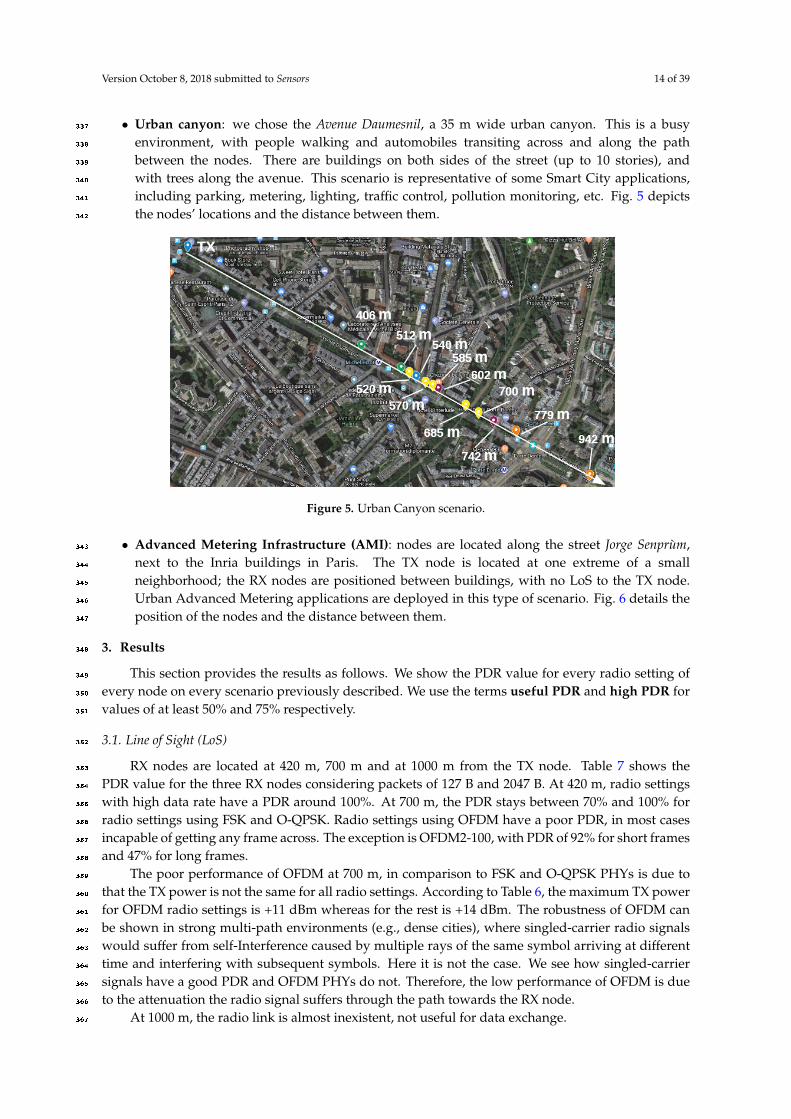
• Urban canyon: we chose the Avenue Daumesnil, a 35 m wide urban canyon. This is a busy337

environment, with people walking and automobiles transiting across and along the path338

between the nodes. There are buildings on both sides of the street (up to 10 stories), and339

with trees along the avenue. This scenario is representative of some Smart City applications,340

including parking, metering, lighting, traffic control, pollution monitoring, etc. Fig. 5 depicts341

the nodes’ locations and the distance between them.342

Figure 5. Urban Canyon scenario.

• Advanced Metering Infrastructure (AMI): nodes are located along the street Jorge Senprùm,343

next to the Inria buildings in Paris. The TX node is located at one extreme of a small344

neighborhood; the RX nodes are positioned between buildings, with no LoS to the TX node.345

Urban Advanced Metering applications are deployed in this type of scenario. Fig. 6 details the346

position of the nodes and the distance between them.347

3. Results348

This section provides the results as follows. We show the PDR value for every radio setting of349

every node on every scenario previously described. We use the terms useful PDR and high PDR for350

values of at least 50% and 75% respectively.351

3.1. Line of Sight (LoS)352

RX nodes are located at 420 m, 700 m and at 1000 m from the TX node. Table 7 shows the353

PDR value for the three RX nodes considering packets of 127 B and 2047 B. At 420 m, radio settings354

with high data rate have a PDR around 100%. At 700 m, the PDR stays between 70% and 100% for355

radio settings using FSK and O-QPSK. Radio settings using OFDM have a poor PDR, in most cases356

incapable of getting any frame across. The exception is OFDM2-100, with PDR of 92% for short frames357

and 47% for long frames.358

The poor performance of OFDM at 700 m, in comparison to FSK and O-QPSK PHYs is due to359

that the TX power is not the same for all radio settings. According to Table 6, the maximum TX power360

for OFDM radio settings is +11 dBm whereas for the rest is +14 dBm. The robustness of OFDM can361

be shown in strong multi-path environments (e.g., dense cities), where singled-carrier radio signals362

would suffer from self-Interference caused by multiple rays of the same symbol arriving at different363

time and interfering with subsequent symbols. Here it is not the case. We see how singled-carrier364

signals have a good PDR and OFDM PHYs do not. Therefore, the low performance of OFDM is due365

to the attenuation the radio signal suffers through the path towards the RX node.366

At 1000 m, the radio link is almost inexistent, not useful for data exchange.367


Table 7. Line-of-Sight. PDR considering packets of 127 B and 2047 B for each RX node. High datarates with high PDR are achieved at least up to 420 m from the TX node. Maximum length of the radiolink is close to 700 m.

RX at 420 m RX at 700 m RX at 1000 mPHY Alias PDR PDR PDR

127 B – 2047 B 127 B – 2047 B 127 B – 2047 B

2FSK-50 100 % – 100 % 83 % – 58 % 0 % – 0 %2FSK-100 100 % – 100 % 76 % – 0 % 0 % – 0 %4FSK-200 100 % – 99 % 0 % – 0 % 0 % – 0 %

2FSK-FEC-50 100 % – 100 % 95 % – 94 % 0 % – 0 %2FSK-FEC-100 100 % – 100 % 100 % – 79 % 0 % – 0 %4FSK-FEC-200 100 % – 100 % 73 % – 38 % 0 % – 0 %

OFDM1-100 100 % – 100 % 31 % – 5 % 0 % – 0 %OFDM1-200 100 % – 100 % 0 % – 18 % 0 % – 0 %OFDM1-400 100 % – 100 % 0 % – 0 % 0 % – 0 %OFDM1-800 100 % – 100 % 0 % – 0 % 0 % – 0 %

OFDM2-50 99 % – 98 % 23 % – 59 % 0 % – 0 %OFDM2-100 100 % – 98 % 92 % – 47 % 0 % – 0 %OFDM2-200 100 % – 100 % 0 % – 0 % 0 % – 0 %OFDM2-400 100 % – 99 % 0 % – 0 % 0 % – 0 %OFDM2-600 100 % – 100 % 0 % – 0 % 0 % – 0 %OFDM2-800 98 % – 51 % 0 % – 0 % 0 % – 0 %

OFDM3-50 100 % – 100 % 34 % – 26 % 0 % – 0 %OFDM3-100 100 % – 100 % 0 % – 0 % 0 % – 0 %OFDM3-200 100 % – 100 % 0 % – 0 % 0 % – 0 %OFDM3-300 100 % – 100 % 0 % – 0 % 0 % – 0 %OFDM3-400 100 % – 97 % 0 % – 0 % 0 % – 0 %OFDM3-600 26 % – 0 % 0 % – 0 % 0 % – 0 %

OFDM4-50 100 % – 98 % 35 % – 11 % 0 % – 0 %OFDM4-100 98 % – 99 % 1 % – 1 % 0 % – 0 %OFDM4-150 100 % – 99 % 8 % – 0 % 0 % – 0 %OFDM4-200 99 % – 100 % 0 % – 0 % 0 % – 0 %OFDM4-300 97 % – 63 % 0 % – 0 % 0 % – 0 %

OQPSK-6.25 100 % – 99 % 100 % – 98 % 27 % – 1 %OQPSK-12.5 100 % – 100 % 94 % – 94 % 2 % – 1 %OQPSK-25 100 % – 100 % 100 % – 83 % 0 % – 0 %OQPSK-50 100 % – 99 % 100 % –100 % 0 % – 0 %


TX

126 m

180 m

350 m

210 m

400 m

215 m

Figure 6. Advance Metering Infrastructure scenario.

3.2. Smart Agriculture Scenario368

In this scenario, the experiment is run twice during the same day and with equal weather369

conditions. RX nodes are located at 213 m, 439 m and 615 m from the TX node on the first run370

and at 337 m, 538 m and 715 m on the second run. Table 8 shows the PDR for all the RX nodes, for371

packets of 127 B and 2047 B. High data rates radio setting with high PDR are achievable at least up to372

337 m. At 615 m, the radio link allows communication of at least 50 kbps with high PDR value. At373

715 m, only OQPSK-12.5 present a high PDR for short packets.374

3.3. Urban Canyon375

In this scenario we collect measurements from 12 locations, between 406 m and 942 m and within376

3 non-consecutive days with similar conditions (sunny days, at noon). Tables 9 and 10 shows the PDR377

for packets of 127 B and 2047 B on each RX node location.378

In this scenario, interference and multi-path fading are expected since this is a high populated379

area with many buildings along the street, with smart metering devices already implemented and380

other applications accessing the same frequency band. As shown in Table 9, the PDR for OFDM2381

is lower at 406 m than at 512 m. An explanation for this is external interference. These two382

measurements were not taken at the same moment, and we can also see that the interference383

was present during the transmission of packets with OFDM2-50, OFDM2-100, OFDM2-200 and384

OFDM2-400. Before and after that time, PDR rose to values close to 100 %. And for the following385

node locations, these high values are maintained.386

After 540 m, there is a negative slope in the street level and after 685 m there is a viaduct which387

is perpendicular to the avenue Daumesnil. High data rates with high PDR are achieved at least up to388

540 m, and the maximum coverage of the radio link is around 780 m.389


Table 8. Smart Agriculture. PDR for packets of 127 B and 2047 B for each RX node. Maximumcoverage with high data rate happens at 337 m and maximum length of the radio link with usefulPDR and data rate of at least 50 kbps is at 615 m.

RX at 213 m RX at 337 m RX at 439 m RX at 538 m RX at 615 m RX at 715 mPHY Alias PDR PDR PDR PDR PDR PDR

127 B – 2047 B 127 B – 2047 B 127 B – 2047 B 127 B – 2047 B 127 B – 2047 B 127 B – 2047 B

2FSK-50 100 % – 96 % 100 % – 100 % 31 % – 33 % 0 % – 0 % 5 % – 11 % 0 % – 0 %2FSK-100 100 % –100 % 100 % – 100 % 0 % – 2 % 0 % – 0 % 0 % – 0 % 0 % – 0 %4FSK-200 99 % –100 % 100 % – 100 % 0 % – 0 % 0 % – 0 % 0 % – 0 % 0 % – 0 %

2FSK-FEC-50 100 % – 98 % 100 % – 100 % 100 % –100 % 0 % – 33 % 98 % – 64 % 0 % – 0 %2FSK-FEC-100 100 % –100 % 100 % – 91 % 85 % – 32 % 23 % – 6 % 0 % – 0 % 0 % – 0 %4FSK-FEC-200 100 % –100 % 100 % – 60 % 0 % – 0 % 0 % – 0 % 0 % – 0 % 0 % – 0 %

OFDM1-100 100 % – 99 % 100 % – 100 % 0 % – 0 % 0 % – 0 % 0 % – 0 % 0 % – 0 %OFDM1-200 100 % – 99 % 100 % – 100 % 0 % – 0 % 0 % – 0 % 52 % – 1 % 0 % – 0 %OFDM1-400 100 % –100 % 100 % – 100 % 0 % – 0 % 0 % – 0 % 0 % – 0 % 0 % – 0 %OFDM1-800 100 % –100 % 100 % – 100 % 0 % – 0 % 0 % – 0 % 0 % – 0 % 0 % – 0 %

OFDM2-50 100 % –100 % 100 % – 100 % 5 % – 5 % 0 % – 0 % 17 % – 14 % 0 % – 0 %OFDM2-100 100 % – 99 % 98 % – 100 % 0 % – 0 % 0 % – 0 % 81 % – 1 % 0 % – 0 %OFDM2-200 73 % – 98 % 100 % – 99 % 0 % – 0 % 0 % – 0 % 0 % – 0 % 0 % – 0 %OFDM2-400 99 % –100 % 100 % – 100 % 0 % – 0 % 0 % – 0 % 0 % – 0 % 0 % – 0 %OFDM2-600 99 % – 99 % 99 % – 100 % 0 % – 0 % 0 % – 0 % 0 % – 0 % 0 % – 0 %OFDM2-800 99 % –100 % 97 % – 40 % 0 % – 0 % 0 % – 0 % 0 % – 0 % 0 % – 0 %

OFDM3-50 100 % –100 % 100 % – 100 % 49 % – 0 % 0 % – 0 % 4 % – 3 % 0 % – 0 %OFDM3-100 100 % –100 % 100 % – 92 % 4 % – 0 % 0 % – 0 % 0 % – 0 % 0 % – 0 %OFDM3-200 100 % –100 % 100 % – 100 % 0 % – 0 % 0 % – 0 % 0 % – 0 % 0 % – 0 %OFDM3-300 100 % –100 % 100 % – 86 % 0 % – 0 % 0 % – 0 % 0 % – 0 % 0 % – 0 %OFDM3-400 100 % – 99 % 99 % – 97 % 0 % – 0 % 0 % – 0 % 0 % – 0 % 0 % – 0 %OFDM3-600 100 % –100 % 84 % – 36 % 0 % – 0 % 0 % – 0 % 0 % – 0 % 0 % – 0 %

OFDM4-50 99 % – 98 % 100 % – 100 % 3 % – 3 % 0 % – 0 % 0 % – 0 % 0 % – 0 %OFDM4-100 100 % –100 % 100 % – 100 % 14 % – 0 % 0 % – 0 % 0 % – 0 % 0 % – 0 %OFDM4-150 100 % – 99 % 100 % – 100 % 0 % – 0 % 0 % – 0 % 0 % – 0 % 0 % – 0 %OFDM4-200 100 % – 99 % 99 % – 95 % 0 % – 0 % 0 % – 0 % 0 % – 0 % 0 % – 0 %OFDM4-300 89 % – 99 % 44 % – 75 % 0 % – 0 % 0 % – 0 % 0 % – 0 % 0 % – 0 %

OQPSK-6.25 100 % –100 % 100 % – 100 % 100 % – 96 % 44 % – 37 % 100 % – 87 % 22 % – 64 %OQPSK-12.5 100 % –100 % 100 % – 100 % 94 % – 97 % 91 % – 31 % 90 % – 90 % 91 % – 35 %OQPSK-25 100 % –100 % 100 % – 100 % 100 % –100 % 47 % – 34 % 92 % –100 % 4 % – 14 %OQPSK-50 100 % –100 % 100 % – 100 % 100 % –100 % 56 % – 13 % 100 % – 99 % 0 % – 34 %


Table 9. Urban Canyon. PDR for packets of 127 B and 2047 B for each RX node, for node locationsfrom 406 m to 585 m. Up to 520 m, all radio settings present a PDR over 50 %. PDR of high data ratesdecay at 540 m.


127 B – 2047 B 127 B – 2047 B 127 B – 2047 B 127 B – 2047 B 127 B – 2047 B 127 B – 2047 B

2FSK-50 100 % – 68 % 100 % – 100 % 100 % – 98 % 95 % – 84 % 7 % – 0 % 92 % – 30 %2FSK-100 100 % – 100 % 100 % – 98 % 100 % – 93 % 99 % – 95 % 41 % – 0 % 89 % – 21 %4FSK-200 94 % – 100 % 100 % – 99 % 93 % – 99 % 98 % – 87 % 0 % – 0 % 0 % – 0 %

2FSK-FEC-50 88 % – 100 % 98 % – 97 % 100 % –100 % 100 % – 93 % 92 % – 84 % 91 % – 86 %2FSK-FEC-100 100 % – 100 % 100 % – 100 % 100 % – 99 % 100 % – 96 % 91 % – 69 % 98 % – 78 %4FSK-FEC-200 100 % – 100 % 100 % – 99 % 100 % –100 % 100 % – 95 % 42 % – 26 % 78 % – 39 %

OFDM1-100 96 % – 99 % 83 % – 89 % 97 % – 85 % 96 % – 80 % 0 % – 0 % 7 % – 0 %OFDM1-200 96 % – 99 % 98 % – 92 % 100 % – 84 % 99 % – 83 % 0 % – 0 % 0 % – 0 %OFDM1-400 90 % – 90 % 36 % – 61 % 99 % – 94 % 97 % – 91 % 0 % – 0 % 0 % – 0 %OFDM1-800 43 % – 87 % 68 % – 68 % 98 % – 98 % 97 % – 79 % 0 % – 0 % 0 % – 0 %

OFDM2-50 72 % – 58 % 97 % – 76 % 97 % – 86 % 97 % – 86 % 1 % – 1 % 6 % – 6 %OFDM2-100 17 % – 59 % 97 % – 88 % 99 % – 93 % 97 % – 86 % 0 % – 0 % 58 % – 4 %OFDM2-200 72 % – 61 % 84 % – 93 % 98 % – 93 % 95 % – 76 % 0 % – 0 % 0 % – 0 %OFDM2-400 41 % – 57 % 40 % – 42 % 99 % – 95 % 91 % – 92 % 0 % – 0 % 0 % – 0 %OFDM2-600 98 % – 98 % 29 % – 0 % 98 % – 97 % 97 % – 88 % 0 % – 0 % 0 % – 0 %OFDM2-800 88 % – 96 % 99 % – 94 % 97 % – 90 % 84 % – 11 % 0 % – 0 % 0 % – 0 %


OFDM4-50 100 % – 100 % 99 % – 100 % 100 % – 99 % 99 % – 91 % 9 % – 0 % 33 % – 8 %OFDM4-100 100 % – 100 % 98 % – 98 % 99 % –100 % 97 % – 96 % 0 % – 0 % 33 % – 0 %OFDM4-150 99 % – 80 % 98 % – 100 % 94 % – 98 % 95 % – 91 % 0 % – 0 % 31 % – 0 %OFDM4-200 100 % – 88 % 99 % – 86 % 100 % – 88 % 93 % – 22 % 0 % – 0 % 0 % – 0 %OFDM4-300 99 % – 99 % 100 % – 92 % 88 % – 72 % 60 % – 31 % 0 % – 0 % 0 % – 0 %

OQPSK-6.25 94 % – 85 % 91 % – 49 % 97 % – 55 % 97 % – 81 % 60 % – 12 % 89 % – 7 %OQPSK-12.5 93 % – 86 % 86 % – 59 % 96 % – 56 % 97 % – 56 % 73 % – 4 % 82 % – 12 %OQPSK-25 95 % – 63 % 91 % – 61 % 96 % – 75 % 95 % – 61 % 23 % – 6 % 57 % – 14 %OQPSK-50 91 % – 74 % 90 % – 76 % 99 % – 86 % 98 % – 84 % 41 % – 19 % 67 % – 48 %


Table 10. Urban Canyon. PDR for packets of 127 B and 2047 B for each RX node for node locationsfrom 602 m to 942 m The limit of the radio link is at 779 m.


127 B – 2047 B 127 B – 2047 B 127 B – 2047 B 127 B – 2047 B 127 B – 2047 B 127 B – 2047 B

2FSK-50 0 % – 0 % 99 % – 94 % 2 % – 0 % 0 % – 0 % 42 % – 0 % 0 % – 0 %2FSK-100 0 % – 0 % 40 % – 0 % 0 % – 0 % 0 % – 0 % 0 % – 0 % 0 % – 0 %4FSK-200 0 % – 0 % 0 % – 0 % 0 % – 0 % 0 % – 0 % 0 % – 0 % 0 % – 0 %

2FSK-FEC-50 15 % – 3 % 100 % – 80 % 100 % – 88 % 0 % – 0 % 66 % – 55 % 0 % – 0 %2FSK-FEC-100 8 % – 0 % 100 % – 46 % 38 % – 4 % 0 % – 0 % 17 % – 0 % 0 % – 0 %4FSK-FEC-200 0 % – 0 % 73 % – 24 % 0 % – 0 % 0 % – 0 % 0 % – 0 % 0 % – 0 %

OFDM1-100 0 % – 0 % 79 % – 53 % 0 % – 0 % 0 % – 0 % 0 % – 0 % 0 % – 0 %OFDM1-200 0 % – 0 % 55 % – 1 % 0 % – 0 % 0 % – 0 % 0 % – 0 % 0 % – 0 %OFDM1-400 0 % – 0 % 0 % – 0 % 0 % – 0 % 0 % – 0 % 0 % – 0 % 0 % – 0 %OFDM1-800 0 % – 0 % 0 % – 0 % 0 % – 0 % 0 % – 0 % 0 % – 0 % 0 % – 0 %



OFDM4-50 0 % – 0 % 93 % – 9 % 0 % – 0 % 0 % – 0 % 0 % – 0 % 0 % – 0 %OFDM4-100 0 % – 0 % 6 % – 1 % 0 % – 0 % 0 % – 0 % 0 % – 0 % 0 % – 0 %OFDM4-150 0 % – 0 % 11 % – 0 % 0 % – 0 % 0 % – 0 % 0 % – 0 % 0 % – 0 %OFDM4-200 0 % – 0 % 0 % – 0 % 0 % – 0 % 0 % – 0 % 0 % – 0 % 0 % – 0 %OFDM4-300 0 % – 0 % 0 % – 0 % 0 % – 0 % 0 % – 0 % 0 % – 0 % 0 % – 0 %

OQPSK-6.25 36 % – 0 % 88 % – 53 % 99 % – 79 % 15 % – 0 % 86 % – 16 % 29 % – 1 %OQPSK-12.5 27 % – 0 % 100 % – 79 % 97 % – 87 % 0 % – 0 % 72 % – 38 % 32 % – 0 %OQPSK-25 8 % – 1 % 98 % – 66 % 92 % – 64 % 0 % – 0 % 73 % – 18 % 0 % – 0 %OQPSK-50 0 % – 1 % 98 % – 73 % 94 % – 76 % 0 % – 0 % 89 % – 48 % 0 % – 0 %


Table 11. AMI. PDR for packets of 127 B and 2047 B long. Even without LOS, high data rates can beachieved up to 215 m with the maximum packet length. At 350 m and 400 m, the PDR decays due tothe multiple buildings between TX and RX nodes.


127 B – 2047 B 127 B – 2047 B 127 B – 2047 B 127 B – 2047 B 127 B – 2047 B 127 B – 2047 B

2FSK-50 100 % – 100 % 100 % –100 % 100 % –100 % 100 % –100 % 0 % – 0 % 0 % – 0 %2FSK-100 100 % – 100 % 0 % – 0 % 100 % –100 % 100 % –100 % 0 % – 0 % 0 % – 0 %4FSK-200 94 % – 98 % 0 % – 1 % 97 % –100 % 97 % –100 % 0 % – 0 % 0 % – 0 %

2FSK-FEC-50 83 % – 92 % 100 % –100 % 100 % –100 % 100 % –100 % 3 % – 5 % 79 % – 17 %2FSK-FEC-100 100 % – 100 % 100 % – 73 % 100 % –100 % 100 % –100 % 0 % – 0 % 0 % – 0 %4FSK-FEC-200 100 % – 100 % 43 % – 0 % 100 % –100 % 100 % –100 % 0 % – 0 % 0 % – 0 %

OFDM1-100 100 % – 100 % 100 % –100 % 100 % – 99 % 100 % –100 % 0 % – 0 % 0 % – 0 %OFDM1-200 100 % – 99 % 100 % –100 % 93 % –100 % 100 % – 98 % 0 % – 0 % 0 % – 0 %OFDM1-400 100 % – 94 % 100 % –100 % 100 % –100 % 100 % –100 % 0 % – 0 % 0 % – 0 %OFDM1-800 31 % – 5 % 100 % –100 % 100 % –100 % 100 % –100 % 0 % – 0 % 0 % – 0 %

OFDM2-50 84 % – 100 % 100 % –100 % 99 % – 99 % 99 % – 83 % 0 % – 0 % 0 % – 0 %OFDM2-100 100 % – 99 % 100 % –100 % 100 % –100 % 100 % –100 % 0 % – 0 % 0 % – 0 %OFDM2-200 99 % – 99 % 100 % – 99 % 100 % –100 % 100 % –100 % 0 % – 0 % 0 % – 0 %OFDM2-400 100 % – 99 % 100 % –100 % 100 % –100 % 100 % –100 % 0 % – 0 % 0 % – 0 %OFDM2-600 97 % – 95 % 99 % –100 % 100 % –100 % 99 % –100 % 0 % – 0 % 0 % – 0 %OFDM2-800 100 % – 100 % 99 % –100 % 100 % –100 % 100 % –100 % 0 % – 0 % 0 % – 0 %

OFDM3-50 100 % – 100 % 100 % –100 % 100 % – 98 % 100 % –100 % 0 % – 0 % 0 % – 0 %OFDM3-100 100 % – 91 % 100 % –100 % 100 % –100 % 100 % –100 % 0 % – 0 % 0 % – 0 %OFDM3-200 100 % – 100 % 29 % – 84 % 100 % –100 % 100 % – 95 % 0 % – 0 % 0 % – 0 %OFDM3-300 100 % – 72 % 100 % – 99 % 100 % –100 % 100 % – 87 % 0 % – 0 % 0 % – 0 %OFDM3-400 100 % – 99 % 100 % –100 % 100 % –100 % 100 % –100 % 0 % – 0 % 0 % – 0 %OFDM3-600 99 % – 91 % 99 % – 93 % 87 % – 76 % 97 % – 94 % 0 % – 0 % 0 % – 0 %

OFDM4-50 100 % – 100 % 99 % –100 % 100 % –100 % 100 % – 98 % 0 % – 0 % 0 % – 0 %OFDM4-100 100 % – 100 % 99 % – 99 % 99 % –100 % 99 % – 99 % 0 % – 0 % 0 % – 0 %OFDM4-150 100 % – 99 % 100 % – 97 % 100 % –100 % 100 % – 98 % 0 % – 0 % 0 % – 0 %OFDM4-200 99 % – 100 % 100 % – 98 % 100 % –100 % 100 % – 99 % 0 % – 0 % 0 % – 0 %OFDM4-300 100 % – 99 % 99 % – 99 % 100 % –100 % 97 % – 99 % 0 % – 0 % 0 % – 0 %

OQPSK-6.25 100 % – 96 % 100 % –100 % 100 % –100 % 100 % –100 % 97 % – 10 % 76 % – 24 %OQPSK-12.5 100 % – 100 % 100 % –100 % 100 % –100 % 100 % –100 % 0 % – 0 % 98 % – 31 %OQPSK-25 100 % – 100 % 100 % –100 % 100 % –100 % 100 % –100 % 3 % – 0 % 98 % – 68 %OQPSK-50 100 % – 100 % 100 % –100 % 100 % –100 % 100 % –100 % 0 % – 0 % 98 % – 78 %

3.4. Advanced Metering Infrastructure390

In this scenario, we run the experiment twice during non consecutive days having similar391

weather conditions. In the first run, RX nodes are located at 126 m, 180 m and 215 m. In the second392

run, RX nodes are located at 210 m, 350 m and 400 m. All nodes located within 215 m, even without393

line of sight, have a PDR close to 100 % for almost all radio settings considering packets of 127 B and394

2047 B.395

There are some buildings between the TX node and the RX nodes located at 350 m and 400 m.396

This severely affects the quality of the radio link. In these two node locations only the O-QPSK radio397

settings and in less proportion the 2FSK-FEC-50 are able to get connectivity. These PHYs happen to398

be the most sensitive of the radio.399

Table 11 shows these PDR values for all the RX nodes.400


4. Analysis401

In this section, we provide an analysis per scenario based on three parameters: PDR, throughput402

and electric charge consumption.403

The first parameter, PDR, tackles latency. Making the assumption that retransmissions do not404

take place right after the failure of a packet exchange, this time between retries increases latency.405

Also, a radio link with high PDR is of utmost interest in order to reduce retransmissions and thus,406

electric charge consumption.407

The second parameter, throughput, takes into account the nominal data rate of each radio setting408

times its PDR. The result is the ‘goodput‘, and with this value we can calculate the maximum amount409

of packets that can be exchanged during a given time.410

European regulation requires the use of this frequency band with a duty cycle < 0.1 %.Accordingly, we calculated the maximum amount of correct packets we could send during one hour,which corresponds to 3.6 s combined transmission time. (1) shows how we calculated this number.

Max_Packets ≤ 3.6 s × DR(B/s)× PDRPacket size(B) + Packet overhead(B)

(1)

where 3.6 s is the maximum time a node can transmit per hour and DR is the nominal data rate411

of the radio setting. Packet size is the length of the data in the PHY (PSDU), and Packet overhead412

includes the PHY header and the Synchronization Header (in the case of FSK and O-QPSK)5 or the413

Short Training Field (STF) and Long Training Field (LTF) (in the case of OFDM). The addition of414

Packet size and Packet overhead result in the total amount of bytes the radio needs to transmit in415

order to send a frame.416

The third parameter, electric charge consumption, is obtained by calculating how much electric417

charge is needed to transmit a single packet. We take into account all radio activity, including the418

packet overhead and packet size (PSDU). Eq. (2) shows how we get the electric charge per packet.419

The ITX value is the current drawn by the radio module when it is in transmission mode (see Table 6).420

Electric charge (Coulombs) ≥ Packet size(B) + Packet overhead(B)DR(B/s)× PDR

× ITX (mA) (2)

We see that the PDR value is present in both (1) and (2). This takes into account the potential421

number of retransmissions needed in order to get one correct packet at the receiver side.422

For each scenario, two node locations are considered: the longer coverage where high data rates423

can be achieved and the maximum coverage of the radio link, despite of the data rate. For these node424

locations, we differentiate short (127 B) and long (2047 B) packets.425

We take the value of 2FSK–50 as a reference because this is the most used configuration in the426

industry for smart metering applications worldwide. In addition, this PHY is the one designated to be427

used as the Common Signaling Mode (CSM) during the Multi-PHY Management procedure defined428

in the standard [20]. Moreover, the 2FSK-50 radio setting is the mandatory mode for the Wi-SUN429

alliance in the US and in Europe.430

In the following graphs, we highlight the highest values of each parameter with dotted bars and431

the reference 2FSK–50 with a striped bar. A dotted line is added as a reference on every figure to easily432

compare the 2FSK–50 kbps radio setting with the rest of the PHYs. Although in most cases 2FSK–50433

delivers a good PDR in comparison with most of the other PHYs, this paper shows that there may434

be more interesting PHYs depending on the constraints of range, throughput, duty cycle and electric435

charge consumption.436

5 The Synchronization Header is composed of a Preamble and a Start of Frame Delimiter (SFD). We consider the shortestpreamble defined in the standard [20] for our calculation.


4.1. Line of Sight Scenario437

High data rates can be achieved up to 420 m, and the maximum length of the radio link with low438

data rates can reach 700 m with a high PDR. There is not useful radio link at 1000 m.439

4.1.1. RX at 420 m440

As shown in Fig. 7(a) for a packet size of 127 B, most of the radio settings have a PDR close441

to 100 %, including the reference 2FSK-50. OFDM3-600 is the only exception, with a 26 % PDR. The442

majority of the radio settings has a high reliability at 420 m with LoS.443

Increasing the packets size to 2047 B, Fig. 7(b) shows that the performance of the radio settings444

is not much affected, with high data rates still having a PDR close to 100 %, including the reference445

2FSK-50. The exception in this case are OFDM2-800, OFDM3-600 and OFDM4-300, the highest data446

rates of OFDM options 2, 3 and 4. One of the reasons is that these PHYs present the lowest sensitivity6447

(-101 dBm, -97 dBm and -101 dBm respectively) of the different OFDM radio settings. The poor448

performance of OFDM3-600 (with a 26 % PDR) could be linked to its low sensitivity, being at least449

4 dB lower than any other OFDM radio setting. The sensitivity for 4FSK-200 is 1 dB lower but the450

TX power is 4 dBm higher. Therefore, the signal at the receiver is 4 dB higher for the 4FSK-200 PHY,451

enough to present a PDR of 100%.452

On the other hand, the rest of the PHYs present high reliability. Thus, we do not highlight any453

particular PHY in Figs. 7(a) and 7(b) since most of them have 100 % PDR.454

Considering throughput, with 127 B packets, Fig. 7(c) clearly shows that OFDM1-800 is the PHY455

than can have the maximum amount of correct packets transmitted within an hour (duty cycle of456

0.1 %), with 1531 packets. The reference value, 2FSK–50, can transmit during the same time just 166457

packets.458

This proportion is maintained with packets of 2047 B, as shown in fig. 7(d). OFDM1-800 stands459

alone with the possibility of transmitting 167 packets against roughly 11 of 2FSK-50 whilst having460

0.1 % duty cycle. Therefore, OFDM1-800 has the capability of transmitting more short and long461

packets than any other PHY within the standard, under the 0.1 % duty cycle regulation and at 420 m462

from the TX. If it is the interest of the user to maximize the amount of packets that can be sent,463

OFDM1-800 or any other OFDM option with high data rate can be used, as figs 7(c) and 7(d) show.464

Fig. 7(e) shows the average electric charge consumption per packet transmitted for all radio465

settings. We can see that high data rates PHYs, mostly OFDM, consume several times less electric466

charge charge that the reference 2FSK-50. The most electric charge efficient is, again, OFDM1-800. It467

consumes 178.6 µC to get a 127 B packet across while 2FSK-50 consumes 1807 µC.468

For long packets, average electric charge consumption is depicted in fig. 7(f). The tendency is469

maintained, high data rates consumed less electric charge than the rest. 2FSK-50 consumes in average470

27.5 mC while OFDM1-800 only 1.637 mC.471

4.1.2. RX at 700 m472

Considering the RX node at 700 m, we approach to the limit of the radio link. Fig. 8 shows that473

high data rates are not capable of delivering any packet, making them unusable for similar distances.474

From Fig. 8(a), with short packets, we see that most OFDM radio settings have a poor or475

inexistent PDR. The reference 2FSK-50 has a PDR of 83 %. Only OFDM2-100 presents a PDR of 92 %.476

O-QPSK radio settings have a high reliability, with 3 out of 4 PDR values of 100 % and the remaining477

(OQPSK-12.5) of 94 %. 2FSK-FEC-100 has 100 % PDR. Therefore, we highlight 2FSK-FEC-100 and478

O-QPSK since they have the highest PDR and highest data rate in their technology.479

6 the lower the sensitivity value is, the higher sensitivity is. e.g., a device A with sensitivity of -110 dBm and another deviceB with sensitivity of -120 dBm, device B has a higher sensitivity than device A.


2FSK

-FEC

-50

2FSK

-FEC

-100

4FSK

-FEC

-200

2FSK

-50

2FSK

-100

4FSK

-200

OFDM

1-10

0OF

DM1-

200

OFDM

1-40

0OF

DM1-

800

OFDM

2-50

OFDM

2-10

0OF

DM2-

200

OFDM

2-40

0OF

DM2-

600

OFDM

2-80

0OF

DM3-

50OF

DM3-

100

OFDM

3-20

0OF

DM3-

300

OFDM

3-40

0OF

DM3-

600

OFDM

4-50

OFDM

4-10

0OF

DM4-

150

OFDM

4-20

0OF

DM4-

300

OQPS

K-6.

25OQ

PSK-

12.5

OQPS

K-25

OQPS

K-50

PHY alias

0

20

40

60

80

100

PDR(

%)

(a) PDR of all radio settings at 420 m from TX with packets of127 B. Except from OFDM3-600, all radio settings have a PDRclose to 100 %.

2FSK

-FEC

-50

2FSK

-FEC

-100

4FSK

-FEC

-200

2FSK

-50

2FSK

-100

4FSK

-200

OFDM

1-10

0OF

DM1-

200

OFDM

1-40

0OF

DM1-

800

OFDM

2-50

OFDM

2-10

0OF

DM2-

200

OFDM

2-40

0OF

DM2-

600

OFDM

2-80

0OF

DM3-

50OF

DM3-

100

OFDM

3-20

0OF

DM3-

300

OFDM

3-40

0OF

DM3-

600

OFDM

4-50

OFDM

4-10

0OF

DM4-

150

OFDM

4-20

0OF

DM4-

300

OQPS

K-6.

25OQ

PSK-

12.5

OQPS

K-25

OQPS

K-50

PHY alias

0

20

40

60

80

100

PDR(

%)

(b) PDR of all radio settings at 420 m from TX with packets of2047 B. OFDM2-800 and OFDM4-300 do not have PDR valuesclose to 100 %. OFDM3-600 has 0 % PDR.

2FSK

-FEC

-50

2FSK

-FEC

-100

4FSK

-FEC

-200

2FSK

-50

2FSK

-100

4FSK

-200

OFDM

1-10

0OF

DM1-

200

OFDM

1-40

0OF

DM1-

800

OFDM

2-50

OFDM

2-10

0OF

DM2-

200

OFDM

2-40

0OF

DM2-

600

OFDM

2-80

0OF

DM3-

50OF

DM3-

100

OFDM

3-20

0OF

DM3-

300

OFDM

3-40

0OF

DM3-

600

OFDM

4-50

OFDM

4-10

0OF

DM4-

150

OFDM

4-20

0OF

DM4-

300

OQPS

K-6.

25OQ

PSK-

12.5

OQPS

K-25

OQPS

K-50

PHY

0

200

400

600

800

1000

1200

1400

1600

max

imum

pac

kets

per

hou

r

(c) Maximum amount of 127 B packets that can be correctlysent per PHY under 0.1 % duty cycle regulation. OFDM1-800can send 1531 packets while 2FSK-50 only 166.

2FSK

-FEC

-50

2FSK

-FEC

-100

4FSK

-FEC

-200

2FSK

-50

2FSK

-100

4FSK

-200

OFDM

1-10

0OF

DM1-

200

OFDM

1-40

0OF

DM1-

800

OFDM

2-50

OFDM

2-10

0OF

DM2-

200

OFDM

2-40

0OF

DM2-

600

OFDM

2-80

0OF

DM3-

50OF

DM3-

100

OFDM

3-20

0OF

DM3-

300

OFDM

3-40

0OF

DM3-

600

OFDM

4-50

OFDM

4-10

0OF

DM4-

150

OFDM

4-20

0OF

DM4-

300

OQPS

K-6.

25OQ

PSK-

12.5

OQPS

K-25

OQPS

K-50

PHY

0

20

40

60

80

100

120

140

160

max

imum

pac

kets

per

hou

r

(d) Maximum amount of 2047 B packets that can be correctlysent per PHY under 0.1 % duty cycle regulation. OFDM1-800can send 167 packets while 2FSK-50 roughly 11.

2FSK

-FEC

-50

2FSK

-FEC

-100

4FSK

-FEC

-200

2FSK

-50

2FSK

-100

4FSK

-200

OFDM

1-10

0OF

DM1-

200

OFDM

1-40

0OF

DM1-

800

OFDM

2-50

OFDM

2-10

0OF

DM2-

200

OFDM

2-40

0OF

DM2-

600

OFDM

2-80

0OF

DM3-

50OF

DM3-

100

OFDM

3-20

0OF

DM3-

300

OFDM

3-40

0OF

DM3-

600

OFDM

4-50

OFDM

4-10

0OF

DM4-

150

OFDM

4-20

0OF

DM4-

300

OQPS

K-6.

25OQ

PSK-

12.5

OQPS

K-25

OQPS

K-50

PHY alias

0

1000

2000

3000

4000

5000

6000

C

(e) Average electric charge consumption per packet of 127 Bcorrectly sent. OFDM1-800 is the most electric charge-efficient,consumes 178.6 µC whereas the reference 2FSK-50 consumes1807 µC.

2FSK

-FEC

-50

2FSK

-FEC

-100

4FSK

-FEC

-200

2FSK

-50

2FSK

-100

4FSK

-200

OFDM

1-10

0OF

DM1-

200

OFDM

1-40

0OF

DM1-

800

OFDM

2-50

OFDM

2-10

0OF

DM2-

200

OFDM

2-40

0OF

DM2-

600

OFDM

2-80

0OF

DM3-

50OF

DM3-

100

OFDM

3-20

0OF

DM3-

300

OFDM

3-40

0OF

DM3-

600

OFDM

4-50

OFDM

4-10

0OF

DM4-

150

OFDM

4-20

0OF

DM4-

300

OQPS

K-6.

25OQ

PSK-

12.5

OQPS

K-25

OQPS

K-50

PHY alias

0

10000

20000

30000

40000

50000

60000

C

(f) Average electric charge consumption per packet of 2047 Bcorrectly sent. OFDM1-800 consumes the lowest amount ofelectric charge per packet, with 1637 µC whereas the reference2FSK-50 consumes 27.5 mC.

Figure 7. Line of Sight, 420 m. The radio link allows the transmission of packets with 2047 B evenwith the highest data rates available with a PDR very close to 100 %. Within this distance, high datarates radio settings maintain high reliability while consuming less electric charge and allowing moredata exchange than low data rates radio settings.


Increasing the packet size to 2047 B, we see from Fig. 8(b) that the PDR slightly drops in480

comparison to small packets. Nonetheless, it is still around 80 % for some radio settings. The481

reference is at 58 % PDR, being matched by OFDM2-50 and outperformed by all O-QPSK PHYs482

and 2FSK-FEC-50 and 2FSK-FEC-100. We highlight the highest PDR of each technology, therefore483

2FSK-FEC-50 and OQPSK-50.484

It is notable that for OFDM2-50, the PDR concerning long packets is 59% whereas for short485

packets is only 23%. This is counterintuitive since short packets should have a higher PDR than long486

packets due to is lower probability of getting a wrong symbol throughout the complete received487

frame. Therefore, this effect can be attributed to interference that occurred only in that precise488

moment. For the following radio setting tested, OFDM2-100, we see how the PDR for short packets489

increased to 92%, using the same frequency as OFDM2-50, which shows that the interference is no490

longer present.491

In [16] we see that a link of 3.5 km can be obtained with this technology. They were in the492

Highlands of Scotland and the router node with that link was located at the top of a hill 7. In our493

case, our link did not arrive to one kilometer, mainly due to the obstacle the ground posses at that494

distance 8.495

Now, considering the maximum amount of packets that can be transmitted under the duty cycle496

regulation with short packets. Fig. 8(c) shows that OFDM2-100 is the radio setting that can send up497

to 285 short packets within an hour. Not far behind we have 4FSK-FEC-200 and 2FSK-100 capable of498

transmitting 239 and 253 short packets per hour. 2FSK-50 can transmit only 138 short packets in the499

same period.500

At this distance from TX, few long packets can be transmitted per hour. The reference 2FSK-50501

can transmit roughly 6 packets per hour while OFDM2-100 and OQPSK-50 just 10. We highlight502

those two PHYs. Therefore, if the user is interested in maximizing the throughput, 4FSK-FEC-200,503

2FSK-100 and OFDM2-100 are the most performing PHYs to do so with short packet. With long504

packets, OFDM2-100 and OQPSK-50.505

Fig. 8(e) shows the average electric charge consumption per packet of 127 B transmitted.506

For short packets, the reference consumes 2178 µC whereas the less power hungry in this case,507

OFDM2-100, consumes 964 µC.508

For long packets, average power consumption is depicted in Fig. 8(f). 2FSK-50 consumes in509

average 47.5 mC. The less electric charge consuming PHYs in this scenario are OFDM2-100 and510

OQPSK-50, with 26.8 mC and 29.1 mC respectively. Should the potential user be focused on reducing511

electric charge consumption, dotted-pattern highlighted bars in Figs. 8(e) and 8(f) depict the less512

electric charge hungry PHYs in this case.513

7 https://mountainsensing.org/deployment/router-nodes/8 the Fresnel radius to that distance is 9.29 m and the nodes are at 1.8 m above the ground.


2FSK

-FEC

-50

2FSK

-FEC

-100

4FSK

-FEC

-200

2FSK

-50

2FSK

-100

4FSK

-200

OFDM

1-10

0OF

DM1-

200

OFDM

1-40

0OF

DM1-

800

OFDM

2-50

OFDM

2-10

0OF

DM2-

200

OFDM

2-40

0OF

DM2-

600

OFDM

2-80

0OF

DM3-

50OF

DM3-

100

OFDM

3-20

0OF

DM3-

300

OFDM

3-40

0OF

DM3-

600

OFDM

4-50

OFDM

4-10

0OF

DM4-

150

OFDM

4-20

0OF

DM4-

300

OQPS

K-6.

25OQ

PSK-

12.5

OQPS

K-25

OQPS

K-50

PHY alias

0

20

40

60

80

100

PDR(

%)

(a) PDR at 700 m from TX with packets of 127 B.Highest reliability achieved with 2FSK-FEC-100, OQPSK-6.25,OQPSK-12.5 and OQPSK-50. The reference has 83 % PDR.OFDM2-100 has also higher reliability than the reference.

2FSK

-FEC

-50

2FSK

-FEC

-100

4FSK

-FEC

-200

2FSK

-50

2FSK

-100

4FSK

-200

OFDM

1-10

0OF

DM1-

200

OFDM

1-40

0OF

DM1-

800

OFDM

2-50

OFDM

2-10

0OF

DM2-

200

OFDM

2-40

0OF

DM2-

600

OFDM

2-80

0OF

DM3-

50OF

DM3-

100

OFDM

3-20

0OF

DM3-

300

OFDM

3-40

0OF

DM3-

600

OFDM

4-50

OFDM

4-10

0OF

DM4-

150

OFDM

4-20

0OF

DM4-

300

OQPS

K-6.

25OQ

PSK-

12.5

OQPS

K-25

OQPS

K-50

PHY alias

0

20

40

60

80

100

PDR(

%)

(b) PDR at 700 m from the TX with packets of 2047 B. Thereference has 58 % PDR, while 2FSK-FEC-50 94 % PDR andOQPSK-50 100 % PDR.

2FSK

-FEC

-50

2FSK

-FEC

-100

4FSK

-FEC

-200

2FSK

-50

2FSK

-100

4FSK

-200

OFDM

1-10

0OF

DM1-

200

OFDM

1-40

0OF

DM1-

800

OFDM

2-50

OFDM

2-10

0OF

DM2-

200

OFDM

2-40

0OF

DM2-

600

OFDM

2-80

0OF

DM3-

50OF

DM3-

100

OFDM

3-20

0OF

DM3-

300

OFDM

3-40

0OF

DM3-

600

OFDM

4-50

OFDM

4-10

0OF

DM4-

150

OFDM

4-20

0OF

DM4-

300

OQPS

K-6.

25OQ

PSK-

12.5

OQPS

K-25

OQPS

K-50

PHY

0

50

100

150

200

250

300

max

imum

pac

kets

per

hou

r

(c) Maximum amount of 127 B packets that can be correctlysent within an hour. 4FSK-FEC-200 and 2FSK-100 can send239 and 253 short packets. OFDM2-100 can send up to 285packets, while the reference only 138 packets.

2FSK

-FEC

-50

2FSK

-FEC

-100

4FSK

-FEC

-200

2FSK

-50

2FSK

-100

4FSK

-200

OFDM

1-10

0OF

DM1-

200

OFDM

1-40

0OF

DM1-

800

OFDM

2-50

OFDM

2-10

0OF

DM2-

200

OFDM

2-40

0OF

DM2-

600

OFDM

2-80

0OF

DM3-

50OF

DM3-

100

OFDM

3-20

0OF

DM3-

300

OFDM

3-40

0OF

DM3-

600

OFDM

4-50

OFDM

4-10

0OF

DM4-

150

OFDM

4-20

0OF

DM4-

300

OQPS

K-6.

25OQ

PSK-

12.5

OQPS

K-25

OQPS

K-50

PHY

0

2

4

6

8

10

max

imum

pac

kets

per

hou

r

(d) Maximum amount of 2047 B packets that can be correctlysent within an hour. OFDM2-100 and OQPSK-50 can send upto 10 packets, while the reference 2FSK-50 just 6 packets.

2FSK

-FEC

-50

2FSK

-FEC

-100

4FSK

-FEC

-200

2FSK

-50

2FSK

-100

4FSK

-200

OFDM

1-10

0OF

DM1-

200

OFDM

1-40

0OF

DM1-

800

OFDM

2-50

OFDM

2-10

0OF

DM2-

200

OFDM

2-40

0OF

DM2-

600

OFDM

2-80

0OF

DM3-

50OF

DM3-

100

OFDM

3-20

0OF

DM3-

300

OFDM

3-40

0OF

DM3-

600

OFDM

4-50

OFDM

4-10

0OF

DM4-

150

OFDM

4-20

0OF

DM4-

300

OQPS

K-6.

25OQ

PSK-

12.5

OQPS

K-25

OQPS

K-50

PHY alias

0

1000

2000

3000

4000

5000

C

(e) Average electric charge consumption per packet of 127 B.OFDM2-100 consumes the less electric charge, 964 µC while2FSK-50 consumes 2178 µC.

2FSK

-FEC

-50

2FSK

-FEC

-100

4FSK

-FEC

-200

2FSK

-50

2FSK

-100

4FSK

-200

OFDM

1-10

0OF

DM1-

200

OFDM

1-40

0OF

DM1-

800

OFDM

2-50

OFDM

2-10

0OF

DM2-

200

OFDM

2-40

0OF

DM2-

600

OFDM

2-80

0OF

DM3-

50OF

DM3-

100

OFDM

3-20

0OF

DM3-

300

OFDM

3-40

0OF

DM3-

600

OFDM

4-50

OFDM

4-10

0OF

DM4-

150

OFDM

4-20

0OF

DM4-

300

OQPS

K-6.

25OQ

PSK-

12.5

OQPS

K-25

OQPS

K-50

PHY alias

0

20000

40000

60000

80000

100000

C

(f) Average electric charge consumption per packet of 2047 B.OFDM2-100 and OQPSK-50 are the less electric charge-hungryradio setting, consuming 26.8 mC and 29.1 mC respectivelywhile 2FSK-50 consumes almost the double, 47.5 mC.

Figure 8. Line of Sight, 700 m. Only O-QPSK and FSK radio settings are able to provide thehighest reliability. This node is close to the limits of the coverage. OFDM radio settings have a poorperformance at this distance, but the difference is that OFDM transmissions are at least 3 dBm weakerthat the rest of the PHYs.

4.2. Smart Agriculture Scenario514

In this scenario, high data rates with high PDR are achieved up to 337 m, and maximum length515

of the radio link is reached around 615 m away from the TX node.516


4.2.1. RX at 337 m517

With a packet size of 127 B, Fig. 9(a) shows the PDR of almost all radio settings are very close518

to 100 %, including those with the highest data rate possible (800 kbps). Increasing the packet size to519

2047 B, Fig. 9(b) shows that the PDR remains 100 % for the majority of the radio settings, including520

OFDM1-800. 2FSK-50 is 100 % in both, with short and long packets, as well as its variations with521

higher data rates. Therefore we do not highlight any other PHY, since the potential user has many522

options to choose a radio setting with 100 % PDR.523

We can see that the PDR values for some radio settings are higher for long packets than short524

packets. This is the case for OFDM2-200 and OFDM4-300 at 213 m, and for OFDM4-300 at 337 m. This525

can be linked to interference. Since we are transmitting packets with only 20 ms separation between526

them, short packets series are more likely to be affected than longer packets by a single transmission527

of a different radio technology device using the same frequency and with a lower data rate9.528

Fig. 9(c) shows the maximum amount of packets that can be transmitted per hour, and we can see529

that OFDM1-800 can transmit up to 1531 packets while the reference 2FSK-50 only 166. We highlight530

OFDM1-800 since it can transmit at least 25 % more packets than any other radio setting, and more531

that 9 times the amount of the reference. Considering long packets, OFDM1-800 has the capability532

of sending the maximum amount of packets per hour, up to 167 packets, while the reference roughly533

11. Fig. 9(d) shows the maximum amount of 2047 B packets that can be delivered at 337 m. In534

consequence, if the potential user wants to maximize the throughput of the nodes separated by a535

similar distance, OFDM1-800 offers the highest throughput.536

Fig. 9(e) depicts the average electric charge consumption per packet the radio needs in order to537

send a 127 B packet. The reference 2FSK-50 needs in average 1800 µC. The lowest amount of electric538

charge needed corresponds to OFDM1-800, with just 178 µC, around ten times less electric charge.539

Other radio settings are also “low energy” such as OFDM2-800 with 215 µC, and OFDM2-600 with540

243 µC.541

In Fig. 9(f), we can see the average electric charge consumed by the TX radio in order to transmit542

a long packet. The radio setting with the smallest electric charge requirement is OFDM1-800, with543

1630 µC in average per a 2047 B transmitted packet. The reference 2FSK-50 consumes 27.5 mA, 16544

times more than OFDM1-800. OFDM2-600 consumes 2200 µC, more than 12 times less than the545

reference. If the potential user wants to increase the lifetime of a battery power node, OFDM1-800 is546

the less electric charge demanding PHY in these conditions.547

4.2.2. RX at 615 m548

At this distance, the overall performance of the radio settings is poor.549

Fig. 10(a) shows the PDR of all radio settings for short frames, where the majority of OFDM and550

FSK radio settings are not able to get any frames across. Only O-QSPK PHYs, 2-FSK-FEC-50 and551

OFDM2-100 have a PDR over 80 %. The reference 2FSK-50 has a negligible PDR, only 5 %.552

PDR values for long packets are shown in Fig. 10(b). Only OQPSK PHYs maintain a high PDR.553

2FSK-FEC-50 drops to 64 % and the reference is only 11 %. Therefore, if the potential user wants to554

have radio links with similar length, 2FSK-FEC-50, OFDM2-100 and any O-QPSK radio setting are555

useful for such requirement with short packets. For long packets, any O-QPSK radio setting is useful.556

It can be seen in Table 8 that the PDR values at 538 m are lower than at 615 m. This seems557

counterintuitive since at further distance, lower should be the power of the received signal and thus,558

the PDR. This assumption is correct in environments where the attenuation of the radio signals are559

only due to distance, without obstacles located between the transmitter and receiver. But this is not560

our case. The obstacles surrounding the RX node located at 538 m and its relative position to the TX561

9 A LoRa packet using Spreading Factor 12 with a 13 B payload has a ToA of 925 ms (LoRa Modem Calculator Tool).


2FSK

-FEC

-50

2FSK

-FEC

-100

4FSK

-FEC

-200

2FSK

-50

2FSK

-100

4FSK

-200

OFDM

1-10

0OF

DM1-

200

OFDM

1-40

0OF

DM1-

800

OFDM

2-50

OFDM

2-10

0OF

DM2-

200

OFDM

2-40

0OF

DM2-

600

OFDM

2-80

0OF

DM3-

50OF

DM3-

100

OFDM

3-20

0OF

DM3-

300

OFDM

3-40

0OF

DM3-

600

OFDM

4-50

OFDM

4-10

0OF

DM4-

150

OFDM

4-20

0OF

DM4-

300

OQPS

K-6.

25OQ

PSK-

12.5

OQPS

K-25

OQPS

K-50

PHY alias

0

20

40

60

80

100

PDR(

%)

(a) Packets of 127 B. Almost all radio settings with a PDR closeto 100 %, including those with the higher data rates.

2FSK

-FEC

-50

2FSK

-FEC

-100

4FSK

-FEC

-200

2FSK

-50

2FSK

-100

4FSK

-200

OFDM

1-10

0OF

DM1-

200

OFDM

1-40

0OF

DM1-

800

OFDM

2-50

OFDM

2-10

0OF

DM2-

200

OFDM

2-40

0OF

DM2-

600

OFDM

2-80

0OF

DM3-

50OF

DM3-

100

OFDM

3-20

0OF

DM3-

300

OFDM

3-40

0OF

DM3-

600

OFDM

4-50

OFDM

4-10

0OF

DM4-

150

OFDM

4-20

0OF

DM4-

300

OQPS

K-6.

25OQ

PSK-

12.5

OQPS

K-25

OQPS

K-50

PHY alias

0

20

40

60

80

100

PDR(

%)

(b) Packets of 2047 B. PDR of some radio settings drops, suchas OFDM2-800, 2FSK-100 and 4FSK-200. The whole OFMDoption 1 PHYs stay at 100 %, as well as the reference 2FSK-50and all the O-QPSK radio settings.

2FSK

-FEC

-50

2FSK

-FEC

-100

4FSK

-FEC

-200

2FSK

-50

2FSK

-100

4FSK

-200

OFDM

1-10

0OF

DM1-

200

OFDM

1-40

0OF

DM1-

800

OFDM

2-50

OFDM

2-10

0OF

DM2-

200

OFDM

2-40

0OF

DM2-

600

OFDM

2-80

0OF

DM3-

50OF

DM3-

100

OFDM

3-20

0OF

DM3-

300

OFDM

3-40

0OF

DM3-

600

OFDM

4-50

OFDM

4-10

0OF

DM4-

150

OFDM

4-20

0OF

DM4-

300

OQPS

K-6.

25OQ

PSK-

12.5

OQPS

K-25

OQPS

K-50

PHY

0

200

400

600

800

1000

1200

1400

1600

max

imum

pac

kets

per

hou

r

(c) Maximum amount of short packets that can be transmittedper hour. OFDM1-800 can transmit up to 1531 packets whilethe reference just 166.

2FSK

-FEC

-50

2FSK

-FEC

-100

4FSK

-FEC

-200

2FSK

-50

2FSK

-100

4FSK

-200

OFDM

1-10

0OF

DM1-

200

OFDM

1-40

0OF

DM1-

800

OFDM

2-50

OFDM

2-10

0OF

DM2-

200

OFDM

2-40

0OF

DM2-

600

OFDM

2-80

0OF

DM3-

50OF

DM3-

100

OFDM

3-20

0OF

DM3-

300

OFDM

3-40

0OF

DM3-

600

OFDM

4-50

OFDM

4-10

0OF

DM4-

150

OFDM

4-20

0OF

DM4-

300

OQPS

K-6.

25OQ

PSK-

12.5

OQPS

K-25

OQPS

K-50

PHY

0

20

40

60

80

100

120

140

160

max

imum

pac

kets

per

hou

r

(d) Maximum amount of long packets that can be transmittedper hour. OFDM1-800 can transmit up to 167 packets, morethan 10 times the reference with just 11 packets.

2FSK

-FEC

-50

2FSK

-FEC

-100

4FSK

-FEC

-200

2FSK

-50

2FSK

-100

4FSK

-200

OFDM

1-10

0OF

DM1-

200

OFDM

1-40

0OF

DM1-

800

OFDM

2-50

OFDM

2-10

0OF

DM2-

200

OFDM

2-40

0OF

DM2-

600

OFDM

2-80

0OF

DM3-

50OF

DM3-

100

OFDM

3-20

0OF

DM3-

300

OFDM

3-40

0OF

DM3-

600

OFDM

4-50

OFDM

4-10

0OF

DM4-

150

OFDM

4-20

0OF

DM4-

300

OQPS

K-6.

25OQ

PSK-

12.5

OQPS

K-25

OQPS

K-50

PHY alias

0

500

1000

1500

2000

2500

3000

3500

4000

C

(e) Average electric charge consumed per 127 B packettransmitted. OFDM1-800 is the less power-hungry, with178 µC consumed, against the 1800 µC needed by 2SFK-50to transmit the same packet. The rest of the high data ratesOFDM PHYs also consume significantly less electric chargethan the reference.

2FSK

-FEC

-50

2FSK

-FEC

-100

4FSK

-FEC

-200

2FSK

-50

2FSK

-100

4FSK

-200

OFDM

1-10

0OF

DM1-

200

OFDM

1-40

0OF

DM1-

800

OFDM

2-50

OFDM

2-10

0OF

DM2-

200

OFDM

2-40

0OF

DM2-

600

OFDM

2-80

0OF

DM3-

50OF

DM3-

100

OFDM

3-20

0OF

DM3-

300

OFDM

3-40

0OF

DM3-

600

OFDM

4-50

OFDM

4-10

0OF

DM4-

150

OFDM

4-20

0OF

DM4-

300

OQPS

K-6.

25OQ

PSK-

12.5

OQPS

K-25

OQPS

K-50

PHY alias

0

10000

20000

30000

40000

50000

60000

C

(f) Average electric charge consumed to sent a long packet.Still OFDM1-800 is the less electric charge-consuming, with1637 µC per packet, whereas the reference consumes 27.5 mC.

Figure 9. Smart Agriculture, 337 m. The PDR for all radio setting considering short and longpackets is high. Using high data rates does not impact in the reliability while reducing electric chargeconsumption and increasing the number of packets exchange within the 0.1 %duty cycle regulation.


node cause this shadowing effect, affecting its PDR. At 615 m, the surroundings of the RX node did562

not have this effect and therefore, the PDR values are higher.563

The maximum amount of short packets that can be sent under the 0.1 % duty cycle regulation564

are shown in Fig. 10(c). Even though OFDM1-200 has only 52 % PDR, its high data rate allows it to565

send just over 300 packets per hour. Not far behind, OFDM2-100 has the possibility of sending up to566

251 packets per hour. 2FSK-50 only 8 packets, and OQPSK-50 below 100 packets of 127 B.567

Now considering long packets, Fig. 10(d) shows the maximum amount each PHY can correctly568

send within an hour. 2FSK-50 can send one long packet per hour, whereas OQPSK-50 just 10. For a569

potential user, if it is wanted to maximize the amount of transmitted packets, OFDM1-200 is the best570

option for short packets. For long packets, OQPSK-50 is the best option but just few packets possible.571

Fig. 10(e) shows the electric charge consumed in average per short packet transmitted to this572

node. 2FSK-50 has a poor PDR, thus the eventual need of retransmissions makes energetically573

expensive to get a packet across. It consumes 36 mC, whereas OFDM1-200 and OFDM2-100 consume574

895 µC and 1095 µC respectively. Therefore, we highlight these last two as the more efficient in electric575

charge consumption. For long packets, Fig. 10(f) shows the average consumption. The reference576

2FSK-50 consumes 250 mC per packet of 2047 B. We can observe that the less consuming PHY is577

OQPSK-50, with 29.5 mC. In both cases, for short and long packets, 2FSK-50 is at least one magnitude578

higher than the most electric charge efficient PHYs.579

4.3. Urban Canyon Scenario580

High data rates with high PDR values are reached up to 540 m away from the TX node. The581

maximum length of the radio link is at 779 m, with important losses at 602 m and 742 m due to582

obstacles and the topography of the scenario.583

4.3.1. RX at 540 m584

PDR values of all radio settings are depicted in Fig. 11(a) for short packets. Overall, all PHYs585

have a high reliability, with values between 84 % and 100 % PDR. The exceptions are OFDM3-600 and586

OFDM4-300, with values of 21 % and 60 % PDR respectively. The reference 2FSK-50 has 95 % PDR.587

We do not highlight any since there are many PHYs with their PDR greater that the reference.588

For long packets, the PDR values are shown in Fig. 11(b). We can see the PDR values decay589

few points, but still several PHYs with higher PDR that the reference (with 84 % PDR). The two590

PHY with highest reliability with long packets are 2FSK-FEC-100 and OFDM4-100 with 95 % and591

96 % PDR respectively. Noticeably, O-QPSK radio settings have a lower PDR, even though their592

sensitivity is higher. Their low data rate makes the time needed to send each frame longer, increasing593

the probabilities of collision with other networks/technologies during transmissions.594

Fig. 11(c) shows the maximum number of packets that can be sent under the 0.1 % duty cycle595

regulation. OFDM1-800 stands alone with the possibility of sending 1485 packets. Some hundreds of596

packets behind, OFDM2-600 and OFDM2-800 with roughly 1115 packets. The reference 2FSK-50 can597

send up to 158 packets per hour.598

Fig. 11(d) shows the maximum number of long packets that can be sent per hour. Still,599

OFDM1-800 is the PHY that allows the maximum number of transmissions per hour, under the duty600

cycle regulation, with roughly 132 packets. OFDM2-600 allows 110 full packet length transmissions,601

while the reference only 9. Consequently, if the potential user wants to maximize the amount of602

packets until the duty cycle regulation limit, OFDM1-800 is shown to be the best for short and long603

packets.604

The average amount of electric charge used to transmit a 127 B packet for all the radio settings605

can be seen in fig. 11(e). The lower electric charge consumption to get one packet across is achieved606

with OFDM1-800, spending 184 µC. The reference 2FSK-50 spends 1900 µC, one magnitude higher.607

Concerning the electric charge consumption for long packets, Fig. 11(f) shows these values. The608

tendency is maintained, OFDM1-800 is the most efficient radio setting to send a packet of 2047 B, with609


2FSK

-FEC

-50

2FSK

-FEC

-100

4FSK

-FEC

-200

2FSK

-50

2FSK

-100

4FSK

-200

OFDM

1-10

0OF

DM1-

200

OFDM

1-40

0OF

DM1-

800

OFDM

2-50

OFDM

2-10

0OF

DM2-

200

OFDM

2-40

0OF

DM2-

600

OFDM

2-80

0OF

DM3-

50OF

DM3-

100

OFDM

3-20

0OF

DM3-

300

OFDM

3-40

0OF

DM3-

600

OFDM

4-50

OFDM

4-10

0OF

DM4-

150

OFDM

4-20

0OF

DM4-

300

OQPS

K-6.

25OQ

PSK-

12.5

OQPS

K-25

OQPS

K-50

PHY alias

0

20

40

60

80

100

PDR(

%)

(a) PDR values for all radio settings with short packets. Only2FSK-FEC-50, OFDM2-100 and all the O-QPSK radio settingshave a PDR over 80 %. The reference has a poor PDR, only5 %.

2FSK

-FEC

-50

2FSK

-FEC

-100

4FSK

-FEC

-200

2FSK

-50

2FSK

-100

4FSK

-200

OFDM

1-10

0OF

DM1-

200

OFDM

1-40

0OF

DM1-

800

OFDM

2-50

OFDM

2-10

0OF

DM2-

200

OFDM

2-40

0OF

DM2-

600

OFDM

2-80

0OF

DM3-

50OF

DM3-

100

OFDM

3-20

0OF

DM3-

300

OFDM

3-40

0OF

DM3-

600

OFDM

4-50

OFDM

4-10

0OF

DM4-

150

OFDM

4-20

0OF

DM4-

300

OQPS

K-6.

25OQ

PSK-

12.5

OQPS

K-25

OQPS

K-50

PHY alias

0

20

40

60

80

100

PDR(

%)

(b) PDR values considering long packets. Only O-QPSK PHYshave PDR values over 85 %, against the reference with 11 %.

2FSK

-FEC

-50

2FSK

-FEC

-100

4FSK

-FEC

-200

2FSK

-50

2FSK

-100

4FSK

-200

OFDM

1-10

0OF

DM1-

200

OFDM

1-40

0OF

DM1-

800

OFDM

2-50

OFDM

2-10

0OF

DM2-

200

OFDM

2-40

0OF

DM2-

600

OFDM

2-80

0OF

DM3-

50OF

DM3-

100

OFDM

3-20

0OF

DM3-

300

OFDM

3-40

0OF

DM3-

600

OFDM

4-50

OFDM

4-10

0OF

DM4-

150

OFDM

4-20

0OF

DM4-

300

OQPS

K-6.

25OQ

PSK-

12.5

OQPS

K-25

OQPS

K-50

PHY

0

50

100

150

200

250

300

max

imum

pac

kets

per

hou

r

(c) Maximum amount of TXs with short packets under0.1 % duty cycle. Despite its PDR of 52 %, OFDM1-200 is ableto transmit up to 300 short packets. The reference can sendjust 8 packets.

2FSK

-FEC

-50

2FSK

-FEC

-100

4FSK

-FEC

-200

2FSK

-50

2FSK

-100

4FSK

-200

OFDM

1-10

0OF

DM1-

200

OFDM

1-40

0OF

DM1-

800

OFDM

2-50

OFDM

2-10

0OF

DM2-

200

OFDM

2-40

0OF

DM2-

600

OFDM

2-80

0OF

DM3-

50OF

DM3-

100

OFDM

3-20

0OF

DM3-

300

OFDM

3-40

0OF

DM3-

600

OFDM

4-50

OFDM

4-10

0OF

DM4-

150

OFDM

4-20

0OF

DM4-

300

OQPS

K-6.

25OQ

PSK-

12.5

OQPS

K-25

OQPS

K-50

PHY

0

2

4

6

8

10m

axim

um p

acke

ts p

er h

our

(d) Maximum amount of TXs with long packets within onehour. OQPSK-50 can send up to 10 long packets while thereference roughly 1 packet per hour.

2FSK

-FEC

-50

2FSK

-FEC

-100

4FSK

-FEC

-200

2FSK

-50

2FSK

-100

4FSK

-200

OFDM

1-10

0OF

DM1-

200

OFDM

1-40

0OF

DM1-

800

OFDM

2-50

OFDM

2-10

0OF

DM2-

200

OFDM

2-40

0OF

DM2-

600

OFDM

2-80

0OF

DM3-

50OF

DM3-

100

OFDM

3-20

0OF

DM3-

300

OFDM

3-40

0OF

DM3-

600

OFDM

4-50

OFDM

4-10

0OF

DM4-

150

OFDM

4-20

0OF

DM4-

300

OQPS

K-6.

25OQ

PSK-

12.5

OQPS

K-25

OQPS

K-50

PHY alias

0

5000

10000

15000

20000

25000

30000

35000

40000

C

(e) Energy consumed per 127 B packet transmitted.OFDM1-200 and OFDM2-100 are the most electriccharge-efficient, consuming 895 µC and 1095 µC respectively.The reference consumes 36 mC. This is due to its poor PDR.

2FSK

-FEC

-50

2FSK

-FEC

-100

4FSK

-FEC

-200

2FSK

-50

2FSK

-100

4FSK

-200

OFDM

1-10

0OF

DM1-

200

OFDM

1-40

0OF

DM1-

800

OFDM

2-50

OFDM

2-10

0OF

DM2-

200

OFDM

2-40

0OF

DM2-

600

OFDM

2-80

0OF

DM3-

50OF

DM3-

100

OFDM

3-20

0OF

DM3-

300

OFDM

3-40

0OF

DM3-

600

OFDM

4-50

OFDM

4-10

0OF

DM4-

150

OFDM

4-20

0OF

DM4-

300

OQPS

K-6.

25OQ

PSK-

12.5

OQPS

K-25

OQPS

K-50

PHY alias

0

100000

200000

300000

400000

500000

600000

C

(f) Energy consumed per 127 B packet transmitted. O-QPSK isthe less electric charge-consuming radio setting, with 29.5 mCwhile the reference consumes 250 mC.

Figure 10. Smart Agriculture, 615 m. The radio link is very close to the maximum distance where itcan deliver connectivity. High data rates OFDM radio settings are unable to get any packet across.Maximum data rate that can provide connectivity is 200 kbps, but with PDR of 52 % with shortpackets.


an average consumption of 2070 µC. OFDM2-600 is close to this value, with 2507 µC per 2047 B sent.610

2FSK-50 consumes, for the same transmission, around 32760 µC.611

4.3.2. RX at 779 m612

At this distance we approach to the limit of the radio link. As shown in Fig. 12(a), only radio613

settings with data rates ≤ 50 kbps present PDR values over 60 % for frames of 127 B. The PDR of614

the reference 2FSK-50 is only 42 %. 2FSK-FEC-50 is the only non O-QPSK PHY with its PDR > 50 %.615

This RX node is located at the limits of the coverage proportionated by the TX node. We can observe616

the PDR values in the fig. 12(b) for packets of 2047 B. Only 2FSK-FEC-50 has a PDR over 50 %. Even617

OQPSK PHYs, with their higher sensitivity, do not have a PDR over 50 %. At this distance and in618

these conditions, only short packets can deliver a good reliability of 80 % with OQPSK-50.619

Fig. 12(c) shows the maximum amount of 1287 B packets that can be sent within an hour under620

the 0.1 % duty cycle regulation. Only OQPSK-50 outperforms the reference, with the possibility of621

sending up to 81 packets per hour against 70 packets of 2FSK-50. For long packets, the maximum622

amount of packets per hour can be seen in fig. 12(d). With a maximum of roughly 5 packets per hour,623

OQPSK-50 is the most convenient PHY. 2FSK-FEC-50 can send up to just 3 full packets and 2FSK-50624

is incapable of get any packet across.625

Fig. 12(e) shows the average electric charge consumed by the TX node in order to get a 127 B626

packet across with the different PHYs. 2FSK-50 consumes 4.3 mC and OQPSK-50 consumes 3.7 mC.627

Any other PHY does not consume less electric charge than those two.628

Similarly but with long packets, we see the electric charge consumption in Fig. 12(f). The TX629

node needs 105 mC to get a packet across when using 2FSK-FEC-50 and 60.7 mC with OQPSK-50. In630

this scenario and at this distance, low data rates and poor PDR make energetically expensive to get631

packets correctly transmitted. If compared with the values at 540 m, at 779 m it is consumed twice632

the electric charge (2FSK-50 at 540 m consumes 32 mC vs OQPSK-50 at 779 m with 60.7 mC).633

In this scenario, we can see results that are counterintuitive:634

For OFDM1-800 and OFDM2 PHYs at 406 m, the PDR is lower for low data rates (50 to 400 kbps)635

than for high data rates (600 and 800 kbps). In interference-and-obstacle-free scenarios, it should636

be the opposite since lower data rates PHYs have a higher sensitivity. This can be attributed to637

interference occurred at the moment of the experiment. This affirmation is backed by the fact that638

for the rest of the radio settings at this distance, the PDR values are above 90%, even for those PHYs639

with lower sensitivity. Same reasoning goes with OFDM2-400 and OFDM2-600 at 512 m.640

Short frames have worst PDR than long frames. The reason is also interference, since a burst of641

short packets can be more affected by a single transmission of different technology/network using a642

lower data rated communication than a long packet burst. We see this more notably in OFDM2-100643

at 406 m and OFDM1-400 at 512 m.644

Nodes located at further distance presenting higher PDR values than nodes located closer to645

the TX node. We are in a scenario where the radio signals interact with trees, people, cars, buses,646

shops, buildings and big metal infrastructure and for some RX locations, these objects are in the way647

between the TX and RX nodes. These objects can cause the shadowing effect of the node, affecting648

the quality of the link between TX and RX and thus, drastically reducing the PDR for that link.649

4.4. Advanced Metering Infrastructure Scenario650

For the nodes located within 215 m, the PDR values of almost all radio settings are close to 100 %.651

Taking one of those 4 locations would have similar results to those exposed in Section 4.3.1. For the652

RX nodes at 350 m and 400 m, PDR values decay and we approach to the limits of the radio link.653

Therefore we present the analysis for those 2 RX locations. Several buildings are between TX and654

those 2 RX nodes, making it a challenging environment to the radio link.655


2FSK

-FEC

-50

2FSK

-FEC

-100

4FSK

-FEC

-200

2FSK

-50

2FSK

-100

4FSK

-200

OFDM

1-10

0OF

DM1-

200

OFDM

1-40

0OF

DM1-

800

OFDM

2-50

OFDM

2-10

0OF

DM2-

200

OFDM

2-40

0OF

DM2-

600

OFDM

2-80

0OF

DM3-

50OF

DM3-

100

OFDM

3-20

0OF

DM3-

300

OFDM

3-40

0OF

DM3-

600

OFDM

4-50

OFDM

4-10

0OF

DM4-

150

OFDM

4-20

0OF

DM4-

300

OQPS

K-6.

25OQ

PSK-

12.5

OQPS

K-25

OQPS

K-50

PHY alias

0

20

40

60

80

100

PDR(

%)

(a) PDR values with packets of 127 B. Overall, high reliabilityexcept for OFDM3-600 and OFDM4-300. Reference value,98 % PDR.

2FSK

-FEC

-50

2FSK

-FEC

-100

4FSK

-FEC

-200

2FSK

-50

2FSK

-100

4FSK

-200

OFDM

1-10

0OF

DM1-

200

OFDM

1-40

0OF

DM1-

800

OFDM

2-50

OFDM

2-10

0OF

DM2-

200

OFDM

2-40

0OF

DM2-

600

OFDM

2-80

0OF

DM3-

50OF

DM3-

100

OFDM

3-20

0OF

DM3-

300

OFDM

3-40

0OF

DM3-

600

OFDM

4-50

OFDM

4-10

0OF

DM4-

150

OFDM

4-20

0OF

DM4-

300

OQPS

K-6.

25OQ

PSK-

12.5

OQPS

K-25

OQPS

K-50

PHY alias

0

20

40

60

80

100

PDR(

%)

(b) PDR values with 2047 B packets. Overall values are over50 %, with few OFDM radio settings. Highest values with2FSK-FEC-100 and OFDM4-100, 95 % PDR and 96 % PDR.Reference value, 84 % PDR.

2FSK

-FEC

-50

2FSK

-FEC

-100

4FSK

-FEC

-200

2FSK

-50

2FSK

-100

4FSK

-200

OFDM

1-10

0OF

DM1-

200

OFDM

1-40

0OF

DM1-

800

OFDM

2-50

OFDM

2-10

0OF

DM2-

200

OFDM

2-40

0OF

DM2-

600

OFDM

2-80

0OF

DM3-

50OF

DM3-

100

OFDM

3-20

0OF

DM3-

300

OFDM

3-40

0OF

DM3-

600

OFDM

4-50

OFDM

4-10

0OF

DM4-

150

OFDM

4-20

0OF

DM4-

300

OQPS

K-6.

25OQ

PSK-

12.5

OQPS

K-25

OQPS

K-50

PHY

0

200

400

600

800

1000

1200

1400

max

imum

pac

kets

per

hou

r

(c) Maximum amount of TX packets of 127 B under the0.1 % duty cycle regulation. OFDM1-800 can transmit up to1485 packets, while the reference 158 packets. OFDM2-600and OFDM2-800 can also transmit more than 1000 shortpackets.

2FSK

-FEC

-50

2FSK

-FEC

-100

4FSK

-FEC

-200

2FSK

-50

2FSK

-100

4FSK

-200

OFDM

1-10

0OF

DM1-

200

OFDM

1-40

0OF

DM1-

800

OFDM

2-50

OFDM

2-10

0OF

DM2-

200

OFDM

2-40

0OF

DM2-

600

OFDM

2-80

0OF

DM3-

50OF

DM3-

100

OFDM

3-20

0OF

DM3-

300

OFDM

3-40

0OF

DM3-

600

OFDM

4-50

OFDM

4-10

0OF

DM4-

150

OFDM

4-20

0OF

DM4-

300

OQPS

K-6.

25OQ

PSK-

12.5

OQPS

K-25

OQPS

K-50

PHY

0

20

40

60

80

100

120

max

imum

pac

kets

per

hou

r

(d) Maximum amount of TX packets of 2047 B under the0.1 % duty cycle regulation. OFDM1-800 can send up to132 packets, OFDM2-600 110 packets and the reference just 9packets.

2FSK

-FEC

-50

2FSK

-FEC

-100

4FSK

-FEC

-200

2FSK

-50

2FSK

-100

4FSK

-200

OFDM

1-10

0OF

DM1-

200

OFDM

1-40

0OF

DM1-

800

OFDM

2-50

OFDM

2-10

0OF

DM2-

200

OFDM

2-40

0OF

DM2-

600

OFDM

2-80

0OF

DM3-

50OF

DM3-

100

OFDM

3-20

0OF

DM3-

300

OFDM

3-40

0OF

DM3-

600

OFDM

4-50

OFDM

4-10

0OF

DM4-

150

OFDM

4-20

0OF

DM4-

300

OQPS

K-6.

25OQ

PSK-

12.5

OQPS

K-25

OQPS

K-50

PHY alias

0

1000

2000

3000

4000

C

(e) Average electric charge consumed per packet of 127 B sent.OFDM1-800 is the less consuming radio setting, with 184 µCper packet whilst 2FSK-50 consumes 1900 µC.

2FSK

-FEC

-50

2FSK

-FEC

-100

4FSK

-FEC

-200

2FSK

-50

2FSK

-100

4FSK

-200

OFDM

1-10

0OF

DM1-

200

OFDM

1-40

0OF

DM1-

800

OFDM

2-50

OFDM

2-10

0OF

DM2-

200

OFDM

2-40

0OF

DM2-

600

OFDM

2-80

0OF

DM3-

50OF

DM3-

100

OFDM

3-20

0OF

DM3-

300

OFDM

3-40

0OF

DM3-

600

OFDM

4-50

OFDM

4-10

0OF

DM4-

150

OFDM

4-20

0OF

DM4-

300

OQPS

K-6.

25OQ

PSK-

12.5

OQPS

K-25

OQPS

K-50

PHY alias

0

10000

20000

30000

40000

C

(f) Average electric charge consumed per packet of 2047 Bsent. OFDM1-800 and OFDM2-600 are the more electriccharge-efficient PHYs, consuming around 2.1 mC and 2.5 mC.2FSK-50 consumes around 33 mC.

Figure 11. Urban Canyon, 540 m. Some high data rate radio settings have a good PDR, close to100 %, and some others suffer from interferences. This is expected in this type of scenarios so an agileMAC layer would be useful in order to overcome those interferences by either changing frequency orwaiting for the availability of the medium.


2FSK

-FEC

-50

2FSK

-FEC

-100

4FSK

-FEC

-200

2FSK

-50

2FSK

-100

4FSK

-200

OFDM

1-10

0OF

DM1-

200

OFDM

1-40

0OF

DM1-

800

OFDM

2-50

OFDM

2-10

0OF

DM2-

200

OFDM

2-40

0OF

DM2-

600

OFDM

2-80

0OF

DM3-

50OF

DM3-

100

OFDM

3-20

0OF

DM3-

300

OFDM

3-40

0OF

DM3-

600

OFDM

4-50

OFDM

4-10

0OF

DM4-

150

OFDM

4-20

0OF

DM4-

300

OQPS

K-6.

25OQ

PSK-

12.5

OQPS

K-25

OQPS

K-50

PHY alias

0

20

40

60

80

PDR(

%)

(a) PDR with packets of 127 B. Only data rates up to 50 kbpsprovide some connectivity, with the exception of O-QPSK-50whose PDR is above 80 %. We are very close to the maximumlength of the radio link. PDR of 2FSK-50 is 42 %.

2FSK

-FEC

-50

2FSK

-FEC

-100

4FSK

-FEC

-200

2FSK

-50

2FSK

-100

4FSK

-200

OFDM

1-10

0OF

DM1-

200

OFDM

1-40

0OF

DM1-

800

OFDM

2-50

OFDM

2-10

0OF

DM2-

200

OFDM

2-40

0OF

DM2-

600

OFDM

2-80

0OF

DM3-

50OF

DM3-

100

OFDM

3-20

0OF

DM3-

300

OFDM

3-40

0OF

DM3-

600

OFDM

4-50

OFDM

4-10

0OF

DM4-

150

OFDM

4-20

0OF

DM4-

300

OQPS

K-6.

25OQ

PSK-

12.5

OQPS

K-25

OQPS

K-50

PHY alias

0

10

20

30

40

50

PDR(

%)

(b) PDR with packets of 2047 B. Only 2FSK-FEC-50 has a PDRover 50 %. The rest of the radio settings does not provide anyconnectivity, with the exception of the O-QPSK radio settings.

2FSK

-FEC

-50

2FSK

-FEC

-100

4FSK

-FEC

-200

2FSK

-50

2FSK

-100

4FSK

-200

OFDM

1-10

0OF

DM1-

200

OFDM

1-40

0OF

DM1-

800

OFDM

2-50

OFDM

2-10

0OF

DM2-

200

OFDM

2-40

0OF

DM2-

600

OFDM

2-80

0OF

DM3-

50OF

DM3-

100

OFDM

3-20

0OF

DM3-

300

OFDM

3-40

0OF

DM3-

600

OFDM

4-50

OFDM

4-10

0OF

DM4-

150

OFDM

4-20

0OF

DM4-

300

OQPS

K-6.

25OQ

PSK-

12.5

OQPS

K-25

OQPS

K-50

PHY alias

01020304050607080

max

imum

pac

kets

per

hou

r

(c) Maximum amount of short packets transmitted per hour.The reference 2FSK-50 can send up to 70 packets andOQPSK-50 81 packets.

2FSK

-FEC

-50

2FSK

-FEC

-100

4FSK

-FEC

-200

2FSK

-50

2FSK

-100

4FSK

-200

OFDM

1-10

0OF

DM1-

200

OFDM

1-40

0OF

DM1-

800

OFDM

2-50

OFDM

2-10

0OF

DM2-

200

OFDM

2-40

0OF

DM2-

600

OFDM

2-80

0OF

DM3-

50OF

DM3-

100

OFDM

3-20

0OF

DM3-

300

OFDM

3-40

0OF

DM3-

600

OFDM

4-50

OFDM

4-10

0OF

DM4-

150

OFDM

4-20

0OF

DM4-

300

OQPS

K-6.

25OQ

PSK-

12.5

OQPS

K-25

OQPS

K-50

PHY alias

0

1

2

3

4

5

max

imum

pac

kets

per

hou

r

(d) Maximum amount of long packets transmitted per hour.OQPSK-50 can send up to 5 2047 B packets per hour under the0.1 % duty cycle regulation.

2FSK

-FEC

-50

2FSK

-FEC

-100

4FSK

-FEC

-200

2FSK

-50

2FSK

-100

4FSK

-200

OFDM

1-10

0OF

DM1-

200

OFDM

1-40

0OF

DM1-

800

OFDM

2-50

OFDM

2-10

0OF

DM2-

200

OFDM

2-40

0OF

DM2-

600

OFDM

2-80

0OF

DM3-

50OF

DM3-

100

OFDM

3-20

0OF

DM3-

300

OFDM

3-40

0OF

DM3-

600

OFDM

4-50

OFDM

4-10

0OF

DM4-

150

OFDM

4-20

0OF

DM4-

300

OQPS

K-6.

25OQ

PSK-

12.5

OQPS

K-25

OQPS

K-50

PHY alias

0

2000

4000

6000

8000

10000

12000

14000

C

(e) Average electric charge consumption per 127 B packet sent.2FSK-50 needs 4.3 mC to transmit one short packet whilstOQPSK-50 consumes 3.7 mC per packet.

2FSK

-FEC

-50

2FSK

-FEC

-100

4FSK

-FEC

-200

2FSK

-50

2FSK

-100

4FSK

-200

OFDM

1-10

0OF

DM1-

200

OFDM

1-40

0OF

DM1-

800

OFDM

2-50

OFDM

2-10

0OF

DM2-

200

OFDM

2-40

0OF

DM2-

600

OFDM

2-80

0OF

DM3-

50OF

DM3-

100

OFDM

3-20

0OF

DM3-

300

OFDM

3-40

0OF

DM3-

600

OFDM

4-50

OFDM

4-10

0OF

DM4-

150

OFDM

4-20

0OF

DM4-

300

OQPS

K-6.

25OQ

PSK-

12.5

OQPS

K-25

OQPS

K-50

PHY alias

0

100000

200000

300000

400000

500000

C

(f) Average electric charge consumption per packet of 2047 Bsent. O-QSPK consumes 60.7 mC, less than any other radiosetting.

Figure 12. Urban Canyon, 779 m. The limit of the radio link is very close to this distance of 779 mfrom the TX node. The PDR for short and long packets is poor, so is the maximum amount of packetsper hour. Applications with short packets and low throughput can stand radio links with similarcharacteristics.


4.4.1. RX at 350 m656

Fig. 13(a) shows the PDR values for all radio settings with a packet length of 127 B. The radio link657

is almost inexistent. Only OQPSK-6.25, the PHY with the slowest data rate available in the standard,658

has a high PDR value, 97 %. The rest of the radio settings have a negligible PDR. Fig. 13(b) depicts the659

poor PDR values with long packets. It is not possible to establish a radio communication with these660

PDR values, which is as high as 10 % for OQPSK-6.25.661

Fig. 13(c) shows the maximum number of packets that can be sent within an hour. OQPSK-6.25662

is capable of delivering roughly 19 short packets. This is enough for some applications where few663

sensor readings are performed per hour. Considering long packets, it is not possible to get even one664

packet across for any PHY, as it is shown in Fig. 13(d).665

The average electric charge consumed to transmit a packet is shown in Fig. 13(e). With666

OQPSK-6.25, the TX node consumes 15.7 mC per packet of 127 B to get correctly sent. For long667

frames, it would take more than 2 C to get a packet across. Therefore, long frames in this scenario are668

not achievable.669


2FSK

-FEC

-50

2FSK

-FEC

-100

4FSK

-FEC

-200

2FSK

-50

2FSK

-100

4FSK

-200

OFDM

1-10

0OF

DM1-

200

OFDM

1-40

0OF

DM1-

800

OFDM

2-50

OFDM

2-10

0OF

DM2-

200

OFDM

2-40

0OF

DM2-

600

OFDM

2-80

0OF

DM3-

50OF

DM3-

100

OFDM

3-20

0OF

DM3-

300

OFDM

3-40

0OF

DM3-

600

OFDM

4-50

OFDM

4-10

0OF

DM4-

150

OFDM

4-20

0OF

DM4-

300

OQPS

K-6.

25OQ

PSK-

12.5

OQPS

K-25

OQPS

K-50

PHY alias

0

20

40

60

80

100

PDR(

%)

(a) PDR values considering packets of 127 B. OnlyOQPSK-6.25 can provide good connectivity with 97 % PDR.The rest of the radio links offers no connectivity at all, PDRvalues of 0 %.

2FSK

-FEC

-50

2FSK

-FEC

-100

4FSK

-FEC

-200

2FSK

-50

2FSK

-100

4FSK

-200

OFDM

1-10

0OF

DM1-

200

OFDM

1-40

0OF

DM1-

800

OFDM

2-50

OFDM

2-10

0OF

DM2-

200

OFDM

2-40

0OF

DM2-

600

OFDM

2-80

0OF

DM3-

50OF

DM3-

100

OFDM

3-20

0OF

DM3-

300

OFDM

3-40

0OF

DM3-

600

OFDM

4-50

OFDM

4-10

0OF

DM4-

150

OFDM

4-20

0OF

DM4-

300

OQPS

K-6.

25OQ

PSK-

12.5

OQPS

K-25

OQPS

K-50

PHY alias

0

2

4

6

8

10

PDR(

%)

(b) PDR values with long packets of 2047 B. The quality of theradio link is overall poor. With PDR values below 10 %, nocommunication link is possible.

2FSK

-FEC

-50

2FSK

-FEC

-100

4FSK

-FEC

-200

2FSK

-50

2FSK

-100

4FSK

-200

OFDM

1-10

0OF

DM1-

200

OFDM

1-40

0OF

DM1-

800

OFDM

2-50

OFDM

2-10

0OF

DM2-

200

OFDM

2-40

0OF

DM2-

600

OFDM

2-80

0OF

DM3-

50OF

DM3-

100

OFDM

3-20

0OF

DM3-

300

OFDM

3-40

0OF

DM3-

600

OFDM

4-50

OFDM

4-10

0OF

DM4-

150

OFDM

4-20

0OF

DM4-

300

OQPS

K-6.

25OQ

PSK-

12.5

OQPS

K-25

OQPS

K-50

PHY

0.0

2.5

5.0

7.5

10.0

12.5

15.0

17.5

20.0

max

imum

pac

kets

per

hou

r

(c) Maximum amount of TX packets per hour. OQPSK-50 canroughly send 19 packets per hour. 2FSK-FEC-50 only 2 andOQPSK-25 only 1. The rest of the PHYs cannot get even onepacket across.

2FSK

-FEC

-50

2FSK

-FEC

-100

4FSK

-FEC

-200

2FSK

-50

2FSK

-100

4FSK

-200

OFDM

1-10

0OF

DM1-

200

OFDM

1-40

0OF

DM1-

800

OFDM

2-50

OFDM

2-10

0OF

DM2-

200

OFDM

2-40

0OF

DM2-

600

OFDM

2-80

0OF

DM3-

50OF

DM3-

100

OFDM

3-20

0OF

DM3-

300

OFDM

3-40

0OF

DM3-

600

OFDM

4-50

OFDM

4-10

0OF

DM4-

150

OFDM

4-20

0OF

DM4-

300

OQPS

K-6.

25OQ

PSK-

12.5

OQPS

K-25

OQPS

K-50

PHY

0.00

0.05

0.10

0.15

0.20

0.25

max

imum

pac

kets

per

hou

r

(d) Maximum amount of TX packets per hour. Any radiosetting is able to send one packet.

2FSK

-FEC

-50

2FSK

-FEC

-100

4FSK

-FEC

-200

2FSK

-50

2FSK

-100

4FSK

-200

OFDM

1-10

0OF

DM1-

200

OFDM

1-40

0OF

DM1-

800

OFDM

2-50

OFDM

2-10

0OF

DM2-

200

OFDM

2-40

0OF

DM2-

600

OFDM

2-80

0OF

DM3-

50OF

DM3-

100

OFDM

3-20

0OF

DM3-

300

OFDM

3-40

0OF

DM3-

600

OFDM

4-50

OFDM

4-10

0OF

DM4-

150

OFDM

4-20

0OF

DM4-

300

OQPS

K-6.

25OQ

PSK-

12.5

OQPS

K-25

OQPS

K-50

PHY alias

0

20000

40000

60000

80000

100000

120000

140000

160000

C

(e) Average electric charge consumed per packet of 127 Btransmitted. OQPSK-6.25 needs 15.7 mC per short packet.

2FSK

-FEC

-50

2FSK

-FEC

-100

4FSK

-FEC

-200

2FSK

-50

2FSK

-100

4FSK

-200

OFDM

1-10

0OF

DM1-

200

OFDM

1-40

0OF

DM1-

800

OFDM

2-50

OFDM

2-10

0OF

DM2-

200

OFDM

2-40

0OF

DM2-

600

OFDM

2-80

0OF

DM3-

50OF

DM3-

100

OFDM

3-20

0OF

DM3-

300

OFDM

3-40

0OF

DM3-

600

OFDM

4-50

OFDM

4-10

0OF

DM4-

150

OFDM

4-20

0OF

DM4-

300

OQPS

K-6.

25OQ

PSK-

12.5

OQPS

K-25

OQPS

K-50

PHY alias

0

500000

1000000

1500000

2000000

C

(f) Average electric charge consumed per packet of 2047 Btransmitted. In average, it takes more than 1 C per packetusing 2FSK-FEC-50 and more than 2 C if OQPSK-6.25 is used.

Figure 13. AMI, 350 m. Only the radio setting OQPSK-6.25 with short packets is useful for this typeof challenging conditions, with several buildings between nodes.

4.4.2. RX at 400 m670

Fig. 14(a) depicts the PDR values for short packets. 2FSK-FEC-50 and O-QPSK PHYs present671

PDR values above 75 %. The rest of the PHYs do not have any reliability, PDR values are zero.672

OQPSK-12.5, OQPSK-25 and OQPSK-50 have 98 % PDR. In Fig. 14(b) is shown the PDR for 2047 B673

packets. The PDR of 2FSK-FEC-50 decays below 20 % while the PDR of OQPSK-50 is still high, at674


78 %. Therefore, the radio setting with the highest reliability for short and long packets is OQPSK-50675

and we highlight it.676

Fig. 14(c) shows the maximum number of short packets that can be transmitted. The radio677

setting that can transmit more packet within one hour is OQPSK-50 with roughly 90 packets. Now678

considering long packets, see Fig. 14(d), OQPSK-50 is still the PHY with a maximum of 8 possible679

packets per hour. Ergo, in order to maximize the throughput of the nodes and being compliant with680

the duty cycle regulation, OQPSK-50 is the most convenient.681

It is depicted in Fig. 14(e) the average electric charge consumed per short packet transmitted. The682

less power-hungry is the OQPSK-50 PHY, with 3.4 mC. Similarly, Fig. 14(f) shows the electric charge683

consumption for long packets. The tendency is maintained, OQPSK-50 consumes the less amount of684

electric charge per 2047 B packet, with 37 mC. Thus, OQPSK-50 is the more electric charge-efficient685

PHY for this scenario, despite of the length of the packet.686


2FSK

-FEC

-50

2FSK

-FEC

-100

4FSK

-FEC

-200

2FSK

-50

2FSK

-100

4FSK

-200

OFDM

1-10

0OF

DM1-

200

OFDM

1-40

0OF

DM1-

800

OFDM

2-50

OFDM

2-10

0OF

DM2-

200

OFDM

2-40

0OF

DM2-

600

OFDM

2-80

0OF

DM3-

50OF

DM3-

100

OFDM

3-20

0OF

DM3-

300

OFDM

3-40

0OF

DM3-

600

OFDM

4-50

OFDM

4-10

0OF

DM4-

150

OFDM

4-20

0OF

DM4-

300

OQPS

K-6.

25OQ

PSK-

12.5

OQPS

K-25

OQPS

K-50

PHY alias

0

20

40

60

80

100

PDR(

%)

(a) PDR values with packets of 127 B. OQPSK-12.5, OQPSK-25and OQPSK-50 have 98 % PDR. We see that the mostadvantageous of that group is OQPSK-50, offering samereliability with higher data rate.

2FSK

-FEC

-50

2FSK

-FEC

-100

4FSK

-FEC

-200

2FSK

-50

2FSK

-100

4FSK

-200

OFDM

1-10

0OF

DM1-

200

OFDM

1-40

0OF

DM1-

800

OFDM

2-50

OFDM

2-10

0OF

DM2-

200

OFDM

2-40

0OF

DM2-

600

OFDM

2-80

0OF

DM3-

50OF

DM3-

100

OFDM

3-20

0OF

DM3-

300

OFDM

3-40

0OF

DM3-

600

OFDM

4-50

OFDM

4-10

0OF

DM4-

150

OFDM

4-20

0OF

DM4-

300

OQPS

K-6.

25OQ

PSK-

12.5

OQPS

K-25

OQPS

K-50

PHY alias

0

10

20

30

40

50

60

70

80

PDR(

%)

(b) PDR values with packets of 2047 B. OQPSK-50 offers thehighest reliability, 78 %, between the 5 radio settings withnon-zero PDR.

2FSK

-FEC

-50

2FSK

-FEC

-100

4FSK

-FEC

-200

2FSK

-50

2FSK

-100

4FSK

-200

OFDM

1-10

0OF

DM1-

200

OFDM

1-40

0OF

DM1-

800

OFDM

2-50

OFDM

2-10

0OF

DM2-

200

OFDM

2-40

0OF

DM2-

600

OFDM

2-80

0OF

DM3-

50OF

DM3-

100

OFDM

3-20

0OF

DM3-

300

OFDM

3-40

0OF

DM3-

600

OFDM

4-50

OFDM

4-10

0OF

DM4-

150

OFDM

4-20

0OF

DM4-

300

OQPS

K-6.

25OQ

PSK-

12.5

OQPS

K-25

OQPS

K-50

PHY

0

20

40

60

80

max

imum

pac

kets

per

hou

r

(c) Maximum amount of TX short packets under 0.1 % dutycycle regulation. O-QPSK-50 can send up to 90 short packets,more than any other radio setting.

2FSK

-FEC

-50

2FSK

-FEC

-100

4FSK

-FEC

-200

2FSK

-50

2FSK

-100

4FSK

-200

OFDM

1-10

0OF

DM1-

200

OFDM

1-40

0OF

DM1-

800

OFDM

2-50

OFDM

2-10

0OF

DM2-

200

OFDM

2-40

0OF

DM2-

600

OFDM

2-80

0OF

DM3-

50OF

DM3-

100

OFDM

3-20

0OF

DM3-

300

OFDM

3-40

0OF

DM3-

600

OFDM

4-50

OFDM

4-10

0OF

DM4-

150

OFDM

4-20

0OF

DM4-

300

OQPS

K-6.

25OQ

PSK-

12.5

OQPS

K-25

OQPS

K-50

PHY

0

1

2

3

4

5

6

7

8

max

imum

pac

kets

per

hou

r

(d) Maximum amount of TX long packets under 0.1 % dutycycle regulation. OQPSK-50 is able to send up to 8 longpackets within one hour.

2FSK

-FEC

-50

2FSK

-FEC

-100

4FSK

-FEC

-200

2FSK

-50

2FSK

-100

4FSK

-200

OFDM

1-10

0OF

DM1-

200

OFDM

1-40

0OF

DM1-

800

OFDM

2-50

OFDM

2-10

0OF

DM2-

200

OFDM

2-40

0OF

DM2-

600

OFDM

2-80

0OF

DM3-

50OF

DM3-

100

OFDM

3-20

0OF

DM3-

300

OFDM

3-40

0OF

DM3-

600

OFDM

4-50

OFDM

4-10

0OF

DM4-

150

OFDM

4-20

0OF

DM4-

300

OQPS

K-6.

25OQ

PSK-

12.5

OQPS

K-25

OQPS

K-50

PHY alias

0

2500

5000

7500

10000

12500

15000

17500

20000

C

(e) Average electric charge consumed per packet of 127 Btransmitted. OQPSK-50 consumes in average, 3.4 mC perpacket transmitted.

2FSK

-FEC

-50

2FSK

-FEC

-100

4FSK

-FEC

-200

2FSK

-50

2FSK

-100

4FSK

-200

OFDM

1-10

0OF

DM1-

200

OFDM

1-40

0OF

DM1-

800

OFDM

2-50

OFDM

2-10

0OF

DM2-

200

OFDM

2-40

0OF

DM2-

600

OFDM

2-80

0OF

DM3-

50OF

DM3-

100

OFDM

3-20

0OF

DM3-

300

OFDM

3-40

0OF

DM3-

600

OFDM

4-50

OFDM

4-10

0OF

DM4-

150

OFDM

4-20

0OF

DM4-

300

OQPS

K-6.

25OQ

PSK-

12.5

OQPS

K-25

OQPS

K-50

PHY alias

0

100000

200000

300000

400000

500000

C

(f) Average electric charge consumed per packet of 2047 Btransmitted. OQPSK-50 is the less electric charge-hungryradio setting, consuming 37 mC per packet transmitted.

Figure 14. AMI, 400 m. It is normal to have several buildings and any other kind of obstacles betweennodes. Having these conditions, the most useful radio setting is OQPSK-50.

5. Discussion687

The lower the frequency, the higher the maximum coverage of the signal with the same TX688

power (considering devices with similar sensitivity). Consequently, the use of a frequency band below689

2.4 GHz increases the range of the radio signals. In comparison with a 2.4 GHz solution, sub-GHz690

enables networks with fewer hops, allowing simpler deployments but with the performance and691

flexibility that mesh networks provide.692


The adoption of the PHYs described in the “g” amendment of IEEE802.15.4 can be beneficial to693

any type of WSN due to the following reasons:694

• They can be used in sub-GHz bands, increasing the range of the radio links.695

• Higher data rates, up to 800 kbps, reduce the transmission/reception time for a packet; this696

lowers the electric charge consumption per byte exchanged and increases the maximum amount697

of packets that can be exchanged considering duty cycle regulations.698

• They provide long range as a Low Power Wide Area Network (LPWAN) combined with the699

flexibility of a mesh network. This enables networks to be built with simple architectures700

(few-hop deep networks) bringing good trade-off between performance and simplicity.701

• The diverse characteristics of each modulation enable further optimization to the low power702

networks solutions. Networks are now able to trade-off data rate, robustness, electric charge703

consumption, range and duty cycle. Choices on the PHY to be used can be made according to704

the current conditions.705

Regulations on sub-GHz bands are in constant revision, which poses an additional challenge to706

keep up with all the evolutions.707

This work is meant to provide the reader a first reference of what can be achieved by the708

IEEE802.15.4g standard in terms of PDR and range on different scenarios where WSN are likely to709

be deployed. We acknowledge that the ideal approach would be to run several times the experiment,710

well separated in time in order to provide results richer in statistical relevance. By doing this, we can711

reduce the impact that transient effects may have in the results. More over, experiments should be712

repeated but the RX nodes should be put half wavelength away in all directions from the selected713

measurement point. This would be useful in order to discard positions where multi-path fading can714

heavily attenuate the radio signal.715

5.1. On the longer range of FSK-FEC and O-QPSK716

Throughout the experiments we can observe that the longest radio links were obtained when717

using the FSK-FEC and O-QPSK PHYs. This is expected as both set of PHYs have the highest718

sensitivity of all PHYs, delivering up to 141 dB of link budget (see Table 6, OQPSK-6.25).719

OFDM radio signals are more robust against interferences and multi-path effects. OFDM1-100720

uses 104 sub-carriers (96 data and 8 pilot tones) with 4x frequency repetition (there are 4 sub-carriers721

with the same information), providing a high level of robustness. OFDM2-50 has the same722

characteristics but half of the sub-carriers and thus, half of the data rate.723

Each OFDM option 1 channel occupies 1.2 MHz and the 4 equal sub-carriers are separated by the724

same distance (in frequency). Even if 3 sub-carriers get compromised during one symbol transmission725

on the path towards the receiver, this can still recover the information. Even though that robustness is726

provided, in Table 7 the PDR for this PHY is just 31% and 5% for short and long packets at 700 m. For727

OFDM2-100, the PDR increased to 92% and 47%. This PHY is 2 dB more sensitive than OFDM1-100.728

We see in Table 6 that the maximum power for OFDM is +11 dBm whereas for the rest is +14dBm.729

Our believe is that the longer range of the O-QPSK and FSK-FEC can be attributed to their higher730

sensitivity in comparison to the rest of the PHYs tested. FSK-FEC holds 5 dB, 5 dB and 8dB higher731

sensitivity than its non-FEC counterpart (2FSK-50, 2FSK-100, 4FSK-200). When compared 2FSK-50732

with OQPSK-50, the difference is 8 dB.733

The reason why OFDM PHYs do not reach as far as these PHYs is that they present a lower734

sensitivity and a lower maximum TX power.735

These values of sensitivity and maximum TX power are directly dependent of the hardware and736

can vary depending on the manufacturer.737


5.2. Future work738

Having such diverse options of PHYs available, it is possible to build a mesh network with739

heterogeneous radio settings. We see the need of designing an agile MAC layer with the following740

characteristics:741

• capable of choosing the most convenient PHY for each pair of nodes.742

• with a Time Slotted Channel Hopping (TSCH) approach, to reduce power consumption by743

eliminating idle listening and reduce collision probabilities. This adds a level of determinism,744

therefore nodes switch on their radios only when their schedule indicate that they are expected745

to transmit/receive frames. The rest of the time nodes can sleep, saving electric charge.746

• a CCA procedure, to be able to increase the duty cycle from 0.1 % to the maximum 2.8 %.747

Conflicts of Interest: The authors declare no conflict of interest.748

Bibliography749

1. Watteyne, T.; Diedrichs, A.L.; Brun-Laguna, K.; Chaar, J.E.; Dujovne, D.; Taffernaberry, J.C.; Mercado, G.750

PEACH: Predicting Frost Events in Peach Orchards Using IoT Technology. EAI Endorsed Transactions on751

the Internet of Things. <hal-01312685> 2016.752

2. Hartung, C.; Han, R.; Seislstad, C.; Holbrook, S. FireWxNet: A Multi-Tiered Portable Wireless System753

for Monitoring Weather Conditions in Wildland Fire Environments. Proceedings of the 4th International754

Conference on Mobile Systems, Applications and Services. ACM, 2006, number 14, pp. 28–41.755

3. Guha, S.K.; Bhaumik, T.K. Design and development of a wireless sensor network for the study of thermal756

instability of the Earth surface as a probable precursor of earthquake. Electronics, Materials Engineering757

and Nano-Technology (IEMENTech) 2017.758

4. Malek, S.; Avanzi, F.; Brun-Laguna, K.; Maurer, T.; Oroza, C.; Hartsough, P.; Watteyne, T.; Glaser, S.759

Real-Time Alpine Measurement System Using Wireless Sensor Networks. Sensors 2017.760

5. IEEE. IEEE Standard for Information Technology - Telecommunications and Information Exchange Between761

Systems - Local and Metropolitan Area Networks Specific Requirements Part 15.4: Wireless Medium Access762

Control (MAC) and Physical Layer (PHY) Specifications for Low-Rate Wireless Personal Area Networks763

(LR-WPANs) IEEE Std 802.15.4-2015, 2015.764

6. Kjeldsen, E.; Hopkins, M. An Experimental Look at RF Propagation in Narrow Tunnels. IEEE Military765

Communications conference 2006.766

7. Zhou, C.; Plass, T.; Jacksha, R.; Waynert, A. RF Propagation in Mines and Tunnels: Extensive767

measurements for vertically, horizontally, and cross-polarized signals in mines and tunnels. IEEE768

Antennas and Propagation Magazine 2015, pp. 88–102.769

8. Thelen, J.; Goense, D.; Langendoen, K. Radio Wave Propagation in Potato Fields. 2005.770

9. Lazarescu, M. Desing and field test of a WSN platform prototype for long-term enviromental monitoring.771

Sensors 2015, pp. 9481–9518.772

10. Cerpa, A.; Busek, N.; Estrin, D. SCALE: A tool for Simple Connectivity Assessment in Lossy773

Environments. Technical report, 2003.774

11. IEEE. IEEE Standard for Local and metropolitan area networks–Part 15.4: Low-Rate Wireless Personal Area775

Networks (LR-WPANs) Amendment 3: Physical Layer (PHY) Specifications for Low-Data-Rate, Wireless, Smart776

Metering Utility Networks. IIEEE Std 802.15.4g-2012 (Amendment to IEEE Std 802.15.4-2011). IEEE, 2012.777

12. Sum, C.S.; Lu, L.; Zhou, M.T.; Kojima, F.; Harada, H. System evaluation of a practical IEEE 802.15.4/4e/4g778

multi-physical and multi-hop smart utility network. 2015, Vol. 9, pp. 665–673.779

13. Dias, J.; Ribeiro, F.; Campos, R.; Ricardo, M.; Martins, L.; Gomes, F.; Carrapatoso, A. Evaluation of an780

RPL/6LoWPAN/IEEE 802.15.4g solution for smart metering in an industrial environment. 12th Annual781

Conference on Wireless On-demand Network Systems and Services (WONS), 2016, pp. 1–4.782

14. Mochizuki, K.; Obatam, K.; Mizutani, K.; Harada, H. Development and Field Experiment of Wide Area783

Wi-SUN System Based on IEEE 802.15.4g. IEEE 3rd World Forum on Internet of Things (WF-IoT)., 2016.784

15. Sum, C.S.; Rahman, M.A.; Lu, L.; Kojima, F.; Harada, H. On Communication and Interference Range of785

IEEE 802.15.4g Smart Utility Networks. IEEE Wireless Communications and Networking Conference 2012.786


16. Bragg, G.M.; Martinez, K.; Basford, P.J.; Hart, J.K. 868MHz 6LoWPAN with ContikiMAC for an Internet787

of Things Environmental Sensor Network. SAI Computing Conference 2016, pp. 1273–1277.788

17. Kojima, F.; Harada, H. Study on Multipath Characteristics for IEEE 802.15.4g SUN Applications in the789

Frequency Band Used in Japan. Communications Workshops. IEEE, 2010.790

18. CEPT-ECC. ERC Recommendation 70-03. Relating to the use of Short Range Devices (SRD). Technical791

report, 2017.792

19. ETSI. Short Range Devices (SRD) operating in the frequency range 25 MHz to 1 000 MHz; Part 1: Technical793

characteristics and methods of measurement, 2017.794

20. IEEE. 802.15.4-2015 - IEEE Standard for Low-Rate Wireless Networks, 2016.795

21. European Telecommunications Standards Institute. Short Range Devices (SRD) operating in the frequency796

range 25 MHz to 1 000 MHz; Part 2: Harmonised Standard covering the essential requirements of article 3.2 of797

Directive 2014/53/EU for non specific radio equipment, 2017.798

22. FCC. 15.247 Operation within the bands 902–928 MHz, 2400–2483.5 MHz, and 5725–5850 MHz, 13.799

23. Association of Radio Industries and Businesses (ARIB). 920MHz-Band Telemeter, Telecontrol and Data800

Transmission Radio Equipment. STD-T108, 2012.801

c© 2018 by the authors. Submitted to Sensors for possible open access publication under the terms and conditions802

of the Creative Commons Attribution license (http://creativecommons.org/licenses/by/4.0/)803

http://creativecommons.org/licenses/by/4.0/.

Documents

Evaluation of IEEE802.15.4g for Environmental Observations