Evaluation of Interestingness and Interaction of Conditions in Discovered Rules:

Applications in Medical Data Analysis

Jerzy Stefanowski Institute of Computing Sciences, Poznań University of Technology Poland

MLLS workshop, Sept. 23, 2016; Riva del Garda

General outline

§  Medical applications of ML

§  Rules induced from data → Interpretation

§  Rule interestingness measures §  Selection of complete rules

§  Another perspective → focus on conditions inside a single rule and in sets of rules

§  Studying most important conditions, their subsets and their interaction in rules

§  Set functions → Shapley and Banzhaf indices, Möbius representation

§  Medical case studies

IF(BAO > 3)THEN disease A IF(vol.ofgastric juice < 150)and(pain = high) THEN disease A IF (Ot.gastric ≥ 100)and(duration=long)THEN disease B

Machine Learning for medical data

§  Machine learning algorithms from beginning applied to analyse medical data

§  Digitalization, new diagnostics tools → facilitate collecting and storing more data

§  Many health units – collect, share large amounts of medical records

§  Interest in automatic deriving medical diagnostic knowledge and interpreting results

See some surveys, such as: I.Konenko: Machine Learning for Medical Diagnosis: History, State of the Art and

Perspectives. R.Bellazzi, F.Felazzi, L.Sachi: Predictive data mining in clinical medicine: a focus

on selected methods and applications. G.Magoulas, A.Prentza: Machine learning in medical applications. …

However, difficulties with clinical acceptance - ECMLPKDD14 tutorial – P.Rodrigues: Knowledge discovery from clinical data

Requirements for systems supporting medical diagnosis

I.Kononeko’s postulates: §  Good performance

§  Dealing with missing data

§  Dealing with noisy data

§  Transparency of diagnostic knowledge

§  Explanation ability

§  Reduction of the number of tests

This paper perspective: →  Symbolic knowledge representation and its interpretation

Usually considered in medicine: Decision trees, rules and partly Bayesian classifiers

Rules – basics

§  Symbolic representation form

IF Conditions THEN Class

§  Natural and easy for human → possible inspection and interpretation → descriptive perspective

§  Individual rules constitute "blocks" of knowledge

§  Rules directly related to facts in the training data

§  Class predictions → easier to justify §  Rules could be integrated with domain knowledge

§  Rules are more flexible than other representations

§  Knowledge representations in AI / Intelligent Systems §  Expert systems, Inference in IS

§  Often used in medical applications

R. Michalski I.Bratko: Machine Learning and Data Mining.; W.Klosgen, J.Zytkow: Handbook of Data Mining and Knowledge Disc; J.Stefanowski: Rule discovery algorithms; C.Aggarwal: Data Classification 2015.

IF Sex = male AND Age > 46 AND

No_of_painful_joints > 3 AND

Skin_manif. = psoriasis THEN Diagnosis =

Crystal_induced_synovitis

Different types of rules

q  Various types of rules in data mining §  Decision / classification rules §  Association rules §  Subgroup discovery → rule patterns §  Logic formulas (ILP) §  Rules in preference learning, rankings and ordinal classification §  Multi-labeled classification §  Sequential rule patterns §  Other → action rules, …

q Other forms of rules in AI or MCDA, q  Comprehensive view:

§  Johannes Fürnkranz, Dragan Gamberger, Nada Lavrač: Foundations of Rule Learning, Springer 2012

How to learn rules?

q  Typical algorithms based on the scheme of a sequential covering and heuristically generate a minimal set of rule to cover learning examples: §  see, e.g., AQ, CN2, LEM, PRISM, MODLEM, Other ideas – PVM, R1,

RIPPER, PART,..

q  Other approaches to induce „richer” sets of rules: §  Satisfying some requirements (Explore, BRUTE, or modification of

association rules → „Apriori-like” CBA, OPUS,…) §  Based on local „reducts” → Boolean reasoning or LDA

q  Optimization problem (MP - Boolean rules) q  Meta-heuristics, e.g., genetic approaches q  Transformations of other representations:

§  Trees → rules §  Construction of (fuzzy) rules from ANN

Case study - buses diagnostic rules

§  A fleet of homogeneous 76 buses (AutoSan H9-21) operating in an inter‑city and local transportation system [ack: J.Zak]

§  76 buses described by 8 technical symptoms and classified into 2 decision classes (good or bad technical condition)

§  Induction of a minimal set of rules (MODLEM) 1. if (s2≥2.4 MPa) & (s7<2.1 l/1000km) then (technical state=good)  [46]

2. if (s2<2.4 MPa) then (technical state=bad)  [29]

3. if (s7≥2.1 l/1000km) then (technical state=bad)  [24]

§  The prediction accuracy → 98.7%.

§  s2 → compression pressure, the most difficult measurement

s1 – maximum speed [km/h] s5 – summer fuel consumption [l/100lm]

s2 – compression pressure [Mpa] s6 – winter fuel consumption [l/100km]

s3 – blacking components in exhaust gas s7 – oil consumption [l/1000km]

s4 – torque [Nm] s8 – maximum horsepower

Another set of rules – describe other conditions

Rules by Explore with threshold (rule coverage > 50% in class): 1. if (s1>85 km/h) then (technical state=good) [34]

2. if (s8>134 kM) then (technical state=good) [26]

3. if (s2≥2.4 MPa) & (s3<61 %) then (technical state=good) [44]

4. if (s2≥2.4 MPa) & (s4>444 Nm) then (technical state=good) [44]

5. if (s2≥2.4 MPa) & (s7<2.1 l/1000km) then (technical state=good) [46]

6. if (s3<61 %) & (s4>444 Nm) then (technical state=good) [42]

7. if (s1≤77 km/h) then (technical state=bad) [25]

8. if (s2<2.4 MPa) then (technical state=bad) [29]

9. if (s7≥2.1 l/1000km) then (technical state=bad) [24]

10. if (s3≥61 %) & (s4≤444 Nm) then (technical state=bad) [28]

11.  if (s3≥61 %) & (s8<120 kM) then (technical state=bad) [27]

More appreciated by domain experts Characteristic description / profile of buses

The prediction accuracy - still 97%

Evaluating conditions in ACL rules

q  Diagnosing of an anterior cruciate ligament (ACL) rupture in a knee on the basis of magnetic resonance (MR) images (Slowinski K. et al. 2002)

q  140 patients described by 6 selected attributes §  age, sex and body side and MR measurements (X, Y and PCL

index) q  Patients categorized into two classes: „1” (with ACL lesion – 100 p.)

and „2” (without ACL – 40 p.)

q  Previous analysis of attribute importance

§  PCLINDEX; then age, sex, side

q  Rule induction → (MODLEM) 15 rules (1- 4 conditions, with different supports)

or richer set of rules (Explore) → over 30 rules

Predictive performance → accuracy 93.5%; G-mean 91.2%

ACL → minimal set of rules

Clinical discussion → MR measurements are the most important. §  In particular, PCL< 3.23 (patients with ACL), PCL ≥ 4.53 (without ACL) §  Other PCL values → combinations with two other attributes age or sex

indicate classes •  Age below 16.5 years (so children or youth) characteristic class

(without ACL lesion) •  ACL injury more frequent for men and right side leg (sportsmen)!

Highly selective vagotomy (HSV) q  Highly selective vagotomy (HSV) - laparoscopic surgery

for perforated Duodenal Ulcer Disease – stomach; q  An attempt to determine indications for HSV treatment

(Slowinski K. et al. 1986);

q  122 patients × 11 pre-operating attributes and assigned to 4 target classes (long term result wrt. Visick grading)

§  Highly imbalanced and complex data

q  LEM2 rule induction algorithm → 44 rules (1- 5 conditions)

q  Predictive performance – accuracy 57% (not the main criterion)

q  Focus on describing characteristic profiles of patients

q  The previous results (e.g. very good prediction – class 1) §  medium or longer duration of the disease, §  without complications of ulcer or acute haemorrhage from ulcer, §  medium or small volume of gastric juice per 1 hour (basic

secretion), §  medium volume of gastric juice per 1 hour under histamine, §  high HCl concentration under histamine.

HSV – patient profiles for other classes

Other classes

q  Satisfactory result of HSV treatment (class 2) §  long or medium duration of disease, §  multiple haemorrhages, §  medium volume of gastric juice per 1 hour (basic secretion), §  medium volume of gastric juice per 1 hour under histamine, §  medium HCl concentration under histamine

q  Unsatisfactory result of HSV treatment (class 3) §  medium or short duration of the disease, §  perforation of ulcer, §  high or small volume of gastric juice per 1 hour (basic secretion), §  high volume of gastric juice per 1 hour under histamine, §  low HCl concentration under histamine.

Motivations for interpreting rule patterns

§  Description perspective → each rule evaluated individually - possibly an „interesting pattern”.

§  Difficulties §  Too many rules to be analyzed!

§  HSV (122 ob.×11 attr.) → 44 rules §  Urology (500 ob. × 33 attr.) → 121 rules

§  Related works → focus interest on some rules: §  Subjective vs. objective perspective §  Rule selection or ordering

§  Studies on rule evaluation measures §  Interactive browsing

§  Need for identification of characteristic attribute value pairs describing patients from particular classes

r1. (A6 = 3) => (D1=1); r2. (A1=2)&(A2=2)&(A4=2)&(A5 =3) => (D1=1); r3. (A1 =2)&(A3=1)&(A4=2) & (A =3) => (D1=1) r4. (A1 = 2) & (A5 = 1) => (D1=2); r5. (A1 = 2) & (A6 = 1) => (D1=2); r6. (A2 = 1) & (A4 = 3) => (D1=2); r7. (A2 = 1) & (A5 = 1) => (D1=2); ………………

Training data

Rule interestingness measures

Rule R: IF P THEN K Objective measures → quantify R with the contingency table (learning data - n)

Many measures → see McGarry, Geng, L., Hamilton, H.et al. surveys; §  Besides support → Bayesian confirmation measures (K,P)

§  Study impact of the rule premise on its conclusion

•  Refer to class probabilities → imbalance

I.Szczech, S.Greco, R.Slowinski: Properties of rule interestingness measures. Inf. Scie. 2012

K ¬K

P a c nP

¬P b d n¬P

nK n¬K n

aRsup =)(

caaRconf+

=)(

naKPG =∧ )(

)()()(),(KGPGKPGQKIND

⋅∧

=

)()|(),( KPPKconfKPC −=

dcc

baaKPPKPPPKN

+−

+=¬−= )|()|(),(

))()|(()()|( KGPKPPGPKK −⋅= α

The best rules according to any monotonic measure are located on the support–anti-support Pareto border

Minority class rules in the support–anti-support evaluation space → transfusion data and BRACID rules [Szczech,Stefanowski]

Toward analysing conditions in rules

Current proposals: → Selecting a subset of rules from a larger set of many rules; → Focus on a „complete” condition part of a rule!

New view → evaluating an importance of elementary conditions and their interaction within the „if” part of the rule

Our aims: §  To propose a new approach based using set functions → Shapley,

Banzhaf indices and Möbius representation §  Start from a single rule → then generalize to the set of rules

§  To verify the approach in rule discovery problems

if p1∧p2∧…∧pn then class K

if (blacking=medium) ∧ (oil_cons=low) ∧ (horsepower=high) then (technical condition = good)

Origins of the proposal

Shapley, Banzhaf indices / values and Möbius representation q  Previously considered in cooperative games, voting systems,

party coalitions and multiple criteria decision aid: q  X = {1,2,...,n} a set of elements / agents

A set function µ : P(X) → [0,1] §  A weighted average contribution of agent / element i in

all coalitions §  Conjoint importance of elements A⊆X §  Measuring interaction of elements

q  Main inspiration (Greco, Slowinski 2001) → a study of the relative value of information supplied by attributes to the quality of classification

Basics q  X = {1,2,...,n} a set of elements (e.g. players in the game);

P(X) – the power set of X = the set of all possible subsets of X A set function µ : P(X) → [0,1]

q  Function µ - a fuzzy measure satisfying: §  µ(∅) = 0 and µ(X) = 1 §  A⊆B implies µ(A) ≤ µ(B) §  „1” could be treated as max value

q  Interpretation of function µ in a particular problem §  The profit obtained by players / agents §  The importance of criteria in MCDA

q  Transformations of function µ §  Shapley and Banzhaf values refer to single elements i ∈ X,

their interactions, subsets of elements A ⊆ X §  Möbius representation m: P(X) → R

Illustrative example – Möbius representation

Möbius representation m: P(X) → R For all A ⊆ X :

§  m(A) – the contribution given by the conjoint presence of all elements from A to the function µ

------------

Consider players 1,2,3, where the profits of their actions are µ({1})=5, µ({2})=7, µ({3})=4 and µ({1,2})=15 (by def. µ(∅)=0)

Calculate m({1})=5, m({2})=7 and m({1,2})=15-5-7=3 Note - µ({1,2})=15 is greater than µ({1} + µ({2})= 5+7 The contribution coming out from the conjoint presence

of {1} and {2} in this coalition and it is equal to m({1,2})=3

)()( ABmAB µ=∑ ⊆

∑ ⊆−−= ABBABAm )1)(()( µ

Illustrative example – Shapley value

§  Shapley value – average contribution / importance of element

§  Consider X={1,2,3} where the profits of the agent actions are µ({1})=5, µ({2})=7, µ({3})=4, µ({1,2})=15, µ({1,3})=12, µ({2,3})=14 and µ({1,2,3})=30

§  How to fairly split the total profit of 30 units among the agents taking into account their contribution?

§  Attribute to the conjoint presence of agents A⊆X, so split equally m(A) among agents

§  Each agent should receive the value (Shapley)

AAm )(

( ) ∑∈⊆

=AiXA

i AAm

:

)(µφ

Illustrative example – Shapley value

§  X={1,2,3} and profits are µ({1})=5, µ({2})=7, µ({3})=4, µ({1,2})=15, µ({1,3})=12, µ({2,3})=14 and µ({1,2,3})=30

Möbius representations §  m({1})=5, m({2})=7, m({3})=4, m({1,2})=µ({1,2})- µ({1}) -µ({2})

=15-5-7=3, m({1,3})=3, µ({2,3})=3 and m({1,2,3})=µ({1,2,3})-µ({1,2})-µ({1,3})-µ({2,3})+µ({1})+ µ({2})+µ({3})=30-15-12-14+5+7+4=5

Shapley values for each agent §  φ1(µ)=m({1})/1+m({1,2})/2+m({1,3})/2+m({1,2,3})/

3=5+3/2+3/2+5/3=9.67 §  φ2(µ)=m({2})/1+m({1,2})/2+m({2,3})/2+m({1,2,3})/

3=7+3/2+3/2+5/3=11.67 §  φ3(µ)=m({3})/1+m({1,3})/2+m({2,3})/2+m({1,2,3})/

3=5+3/2+3/2+5/3=9.67 ( ) ∑

∈⊆=

AiXAi A

Am:

)(µφ

Other formulations

Shapley value:

Banzhaf value:

Both interpreted as an averaged contribution of element i to all coalitions A Interaction indices (i,j) → Morofushi and Soneda; Roubens

)](}){([!

!)!1()( }{ AiA

XAAX

iXAi µµµ −∪⋅−−

=Φ ∑ −⊆

∑ −⊆−+∪−∪−∪= },{2 )](}){(}){(}),{([

21),( jiXAnR AjAiAjiAjiI µµµµ

)](}){([21)( }{2 AiAiXAXiB µµµ −∪=Φ ∑ −⊆−

)](}){(}){(}),{([)!1(

!)!2(),( },{ AjAiAjiA

XAAX

jiI jiXAMS µµµµ +∪−∪−∪⋅−

−−=∑ −⊆

Adaptation to evaluate conditions in a single rule

§  Consider a single rule if p1∧p2∧…∧pn then class K

§  Need to analyse its sub-rules if pj1∧pj2∧…∧pjl then class K such that {pj1,pj2,…,pjl } ⊆ {p1,p2,…,pn }

§  sub-rules are more general than the first rule

§  Choice of the characteristic function µ to evaluate a rule?

§  Confidence of the rule µ(W,K)=conf(r), where W is a set of conditions in r

§  Also – confirmation measures, …

§  Then, for Y ⊂ W we need to adapt set functions

§  µ(∅,K)=? O or class prior

Indices for each condition in a rule

pi∈W - single condition in rule r, and |W| = n §  Shapley value:

§  Banzhaf value:

Both values Φ – a weighted contribution of pi in rules generalized from r For Shapley value - µ(W) is shared among all elements of W Pairs – measures of an interaction resulted from putting pi and pj together

in all subsets of conditions in rule r: •  Positive – complementary in increasing the confidence •  Negative – putting together provide some redundancy

)],()},{([!

!)!1(),( }{ KYKpY

nYYn

rp iipWYis µµ −∪⋅−−

=Φ ∑ −⊆

∑ −⊆−−∪=Φ }{1 )],()},{([

21),(

ipWY iniB KYKpYrp µµ

)],(}){()},{()},,{([)!1(

!)!2(),( },{ KYpYKpYKppY

nYYn

ppI jijijpipWYjiMS µµµµ +∪−∪−∪⋅−

−−=∑ −⊆

Adapted indices for subsets - part 2

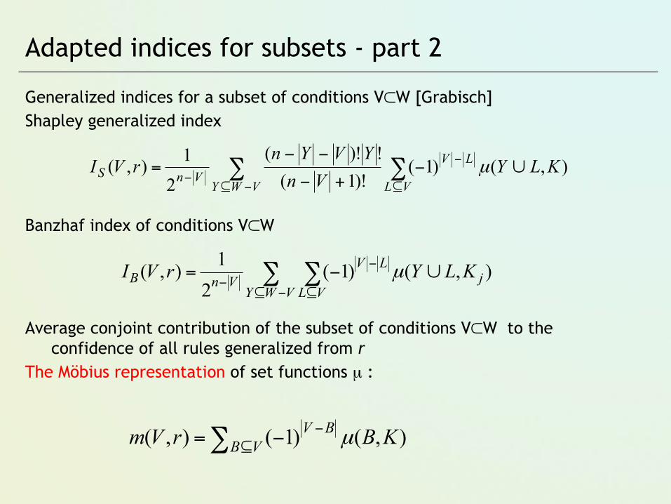
Generalized indices for a subset of conditions V⊂W [Grabisch] Shapley generalized index

Banzhaf index of conditions V⊂W

Average conjoint contribution of the subset of conditions V⊂W to the confidence of all rules generalized from r

The Möbius representation of set functions µ :

∑ ∑−⊆ ⊆

−−

∪−=VWY VL

jLV

VnB KLYrVI ),()1(21),( µ

∑ ∑−⊆ ⊆

−−

∪−+−

−−=

VWY VL

LVVnS KLY

VnYVYn

rVI ),()1()!1(!)!(

21),( µ

∑ ⊆−−= VBBV KBrVm ),()1(),( µ

An intuitive example

HSV treatment – one of the rules if (gastric_juice=medium)∧(HCL_conc.=low) then (result=good)

conf=1.0 , supp = 13 examples.

Möbius representation m(1,2) = -0.14493!!!

§  Rule generalizations and Möbius representation m: §  Empty condition part → m(0)=0 §  if (gastric_juice=medium) then (result =good)

m(1)=0.16667 and conf=0.16667 §  if (HCL_conc.=low) then (result =good)

m(2)=0.97826 and conf= 0.97826 §  An increase of rule confidence

1 = m(1) + m(2) + m(1,2) §  Values of Möbius representation show the distribution of confidence among

all coalitions of the considered conditions in the subset {(gastric_juice=medium),(HCL_conc.=low)}

Shapley value for single conditions ϕ(gastric_juice=medium)=0.0942; ϕ((HCL_conc.=low) =0.908

Evaluating conditions in ACL rule if (sex = female)∧(Y1 < 2.75) ∧( PCL∈[3.71,4.13)) then (no ACL) conf. =1.0

Sex Y1 PCL Banzhaf Shapley Mobius conf.

∅ ∅ √ 0.43535 0.49575 0.28571 0.2857

∅ √ ∅ 0.24207 0.30246 0.04651 0.0465

∅ √ √ 0.53015 0.53015 0.1766 0.5241

√ ∅ ∅ 0.14139 0.1591 0.1452 0.1452

√ ∅ √ 0.1135 0.1135 -0.2316 0.2923

√ √ ∅ 0.1734 0.1734 -0.1034 0.1486

√ √ √ 0.72476 0.72476 0.72476 1

Evaluating conditions in a set of rules

§  The set of rules , where R(Kj) a set of rules having as a consequence class Kj

§  A given set of conditions Γf occur in many rules

§  denote an evaluation of its contribution to the confidence of rule r

§  The global contribution of Γf in a rule set R with respect to class Kj is calculated as:

§  Conditions Γf are ranked according to → identify the most characteristic combinations of conditions for rules from a given class

§  Computational costs → start from the smallest sets of cond.

∪kj jKRR 1 )(==

∑∑ ¬∈∈ ⋅Γ−⋅Γ=Γ )()( )sup()()sup()()( KjRs fsKjRr frjKj sFMrFMG

)( frFM Γ

)( fKjG Γ

An illustrative example

An interest in condition (a7=0) in a set of several rules

It occurs in following rules with conf=1: R1 if (a3=1)∧(a7=0) ∧(a3=1) then (D=1) sup 1

R2 if (a4=1)∧(a7=0) then (D=1) sup 45

R5 if (a4=0)∧(a7=0) then (D=2) sup 7

(Möbius representation of (a7=0)) in R1, R2 m=0.939 and in R5 m=0.184

A global contribution of (a7=0)

§  (D=1) 0.939×1 + 0.939 × 45 = 43.194

§  (D=2) 0.184 ×7 = 1.288

Finally GD=1(a7=0) = 43.194 – 1.288 = 41.906

Analysis of conditions in buses rules

q  Pairs of conditions – much lower evaluations e.g. (horsepower=average) and (oil consumption=low) 0.166

q  Previous analysis → „good” conditions: high compression pressure, torque, max-speed and low blacking components. Opposite values → characteristic for bad technical conditions. Blacking components in the exhaust gas and oil consumption more important than fuel consumption.

Evaluating conditions in ACL rules q  Diagnosing an anterior cruciate ligament (ACL) rupture in a knee on the

basis of magnetic resonance (MR) images (Slowinski K. et al.)

q  140 patients described by 6 attributes §  age, sex and body side and MR measurements (X, Y and PCL index).

q  Patients classified into two classes „1” (with ACL lesion – 100) and „2” (without ACL – 40).

q  LEM2 rule induction algorithm → 15 rules (1- 4 elementary conditions with different support, few possible rules).

q  Clinical discussion → MR measurements are the most important. §  In particular PCL< 3.23 (patients with ACL), PCL ≥ 4.53 (without ACL) §  Other PCL values → combinations with two other attributes age or

sex indicate classes. §  Age below 16.5 years (so children or youth) characteristic

for class (without ACL lesion). §  ACL injury more frequent for men (sportsmen)!

ACL → minimal set of rules

Evaluating conditions in ACL rules

Subsets of conditions → characteristic description of both diagnostic classes; PCL index with extreme intervals definitely the most important + its other values occur in some pairs, e.g (Age∈[16.5,35]) & (PCL ∈ [3.7,4.1) Sex and age – young men (often sportsmen)

With ACL Without ACL Möbius Shapley Möbius Shapley

PCL < 3.23 18.57 PCL < 3.23 18.57 PCL ≥ 4.53 21.42 PCL ≥ 4.53 21.42

PCL∈[3.23,3.7) 4.87 PCL∈[3.23,3.7) 5.06 Age < 16.5 4.0 Age < 16.5 4.0

(Age∈[16.5,35] & (PCL ∈[3.7,4.1)

1.58 Age∈[16.5,35) 1.63 Sex=female 3.23 Sex=female 2.85

(X1≥14.5) & (PCL ∈[3.7,4.1)

0.54 (X1≥14.5) & (PCL ∈[3.7,4.1)

0,92 PCL∈[4.13,4.5) 2.22 Y1∈[2.75,3.75) 1.84

X1 ∈[8.5,11.8) 0.52 Age∈[16.5,35 & (PCL ∈[3.7,4.1)

0.86 (Age≥35] & (PCL ∈[3.7,4.1)

1.78 (Age≥35] & (PCL ∈[3.7,4.1)

1.78

Sex=male 0.44 Sex=male 0.83 X1∈[11.8,14.5)PCL∈[3.23,3.7)

1.31 X1∈[11.8,14.5) 1.53

Age∈[16.5,35) 0.34 Y1<2,75 & (PCL ∈[3.7,4.1)

0.67 Y1∈[2.75,3.75) 1.28 PCL∈[4.13,4.53 1.48

Evaluating conditions in ACL rules

q  Rankings of conditions with respect to Shapley and Banzhaf values – top elements are the same.

q  Top ranking with Möbius representation small re-ordering but PCL also dominates

q  Pairs of conditions are higher evaluated than in the previous case

q  Support for profiles of ACL patients

§  MR measurements are the most important

Patients with ACL §  PCL< 3.23 ; (Age∈[16.5,35]) & (PCL ∈ [3.7,4.1) §  Sex=male and X1 ∈[8.5,11.8) Patients without ACL §  PCL ≥ 4.53 §  Other MR measurements → combinations with two other attributes

age or sex indicate classes. §  Age below 16.5 years (so children or youth) or (age = much older)

are characteristic for (without ACL) q  Profiles consistent with the earlier analyses and clinical knowledge

Highly selective vagotomy rules

Highly selective vagotomy (HSV) - laparoscopic surgery for perforated Duodenal Ulcer Disease.

q  An attempt to determine indications for surgery treatment;

§  122 patients described by 11 pre-operating attributes and assigned to 4 target class

§  44 rules (1- 5 conditions)

q  Focus on describing characteristic profiles of patients

q  The previous results, e.g. very good prediction – class 1) §  long or medium duration of the disease, §  without complications of ulcer or acute haemorrhage from ulcer, §  medium or small volume of gastric juice per 1 hour (basic

secretion), §  medium volume of gastric juice per 1 hour under histamine, §  high HCl concentration under histamine.

Evaluating conditions in HSV rules – class 1 (good)

Attributes: A2 – age; A4 – complications of ulcer; A6 - volume of gastric juice per h; A9 - HCL concentration after histamine; A5 - HCL concentration; A3 - duration of disease

Subsets of conditions → closer to single conditions

Möbius Shapley Banzhaf

Cond Value Cond Value Cond Value

A6=2 2,34 A6=2 3,85 A6=2 4,01

A9=3 2,31 A4=1 3,41 A4=1 3,57

A4=2 1,89 A4=2 3,16 A4=2 3,08

A4=1 1,58 A9=3 2,59 A9=3 2,72

A2=2 1,27 A2=2 1,65 A2=2 1,88

Möbius Shapley Banzhaf Cond Value Cond Value Cond Value

A4=1 & A6=2 2,62 A4=1 & A6=2 2,82 A4=1 & A6=2 2,83

A4=1 & A8=1 1,95 A4=1 & A8=1 1,95 A4=1 & A8=1 1,95

A2=2 & A6=2 1,89 A5=2 & A6=1 1,49 A5=2 & A6=1 1,49

A2=2 & A9=3 1,53 A3=3 & A7=2 1,18 A3=3 & A7=2 1,18

A5=2 & A6=1 1,49 A2=2 & A6=2 1,01 A2=2 & A6=2 1,01

HSV –patient class profiles q  Very good result of HSV (class 1)

§  without complications of ulcer or acute haemorrhage from ulcer,

§  medium or small volume of gastric juice per 1 hour (basic secretion),

§  medium volume of gastric juice per 1 hour under histamine,

§  high HCl concentration under histamine

§  / no medium duration of disease

q  Satisfactory result of HSV (class 2) §  long or medium duration of disease, §  multiple haemorrhages, §  medium or small volume of gastric

juice per 1 hour (basic secretion), §  medium volume of gastric juice per 1

hour under histamine, §  medium or low HCl concentration

under histamine

q  Unsatisfactory result of HSV treatment (class 3) §  medium or short duration of the

disease, §  perforation of ulcer, §  high or small volume of gastric

juice per 1 hour (basic secretion),

§  high volume of gastric juice per 1 hour under histamine,

§  No low HCl concentration under histamine condition in the rankings

q  Bad result of HSV treatment (class 4) §  Consistent profile §  + new condition - low HCl

concentration under histamine

Working with larger set of rules

q  „ESWL” – urological data §  Urinary stones treatment by ESWL extracorporeal shock waves

lithotripsy q  500 patients × 33 attributes classified into two classes

(imbalanced) – difficult to analyse (Antczak, Kwias et al. 2000) q  Explore rule induction algorithm → 484 rules (2-7 conditions with

different support ≥ 5%, confidence ≥ 0.8).

ESWL rules

q  Explore rule induction algorithm → 484 rules (2-7 conditions with different support ≥ 5%, confidence ≥ 0.8).

q  Using the set functions we identify: §  Class 1 → 8 single conditions, 12 pairs

•  (basic dysuric symptoms=1), (crystaluria=1), (location of the concrement=2),(stone size=2), …, (crystaluria=2)&(proteinurine=1), etc.

§  Class 2 → 10 single conditions, 13 pairs •  (location of the concrement =3), (lumbar region pains=5),

(operations in the past=3),…, (crystaluria=3)&(proteinurine=2),..,(cup-concrement=1)&(stone size=2), etc.

q  More visible differences in Shapley and Banzhaf rankings ; triples less evaluated than single conditions and pairs.

Extensions to improve computability

§  Limitations - computational for rules having more conditions

§  Both time and memory (to store temporary results)

§  Possible heuristic approaches:

§  First filter and reduce the set of rules, then evaluate.

§  Iterative analysis, start from single conditions, pairs and work with smaller sets of conditions

§  Modify calculations of measures (approximate them)

M.Sikora: Selected methods for decision rule evaluation and pruning (2013)

§  Analyse only single conditions in rules

§  Do not consider all sub-rules (restrict to rules affected by dropping the single condition, or base sub-rules with the single condition)

§  Simpler forms of Baznhaf and Shapley indices

Possible re-using of best conditions in rule constructive induction

Final remarks

Interpretation of rule patterns Our contribution: §  Evaluating the role of subsets of elementary conditions in rules discovered

from data + their interaction and conjoint contribution §  An adaptation of measures based on set functions (not so frequent in ML)

Medical context: §  Identification of the most important conditions in single rules, sets of rules §  Support for characteristic descriptions of patients from different targets §  Using rules → order of applying diagnostic tests inside rules, complementary

tests (use together), redundancy,..

Experimental observations: §  Identified conditions, pairs consistent with previous results (4 case studies) §  Rankings quite similar: Möbius has a wider range, Shapley and Banzhaf nearly

the same – differences for larger sets of rules having more conditions

Approximate calculations + other applications

Co-operation with

Rules and set functions: Salvatore Greco (University of Catania) and Roman Słowiński (Poznan University of Technology)

S.Greco, R.Slowinski, J.Stefanowski: Evaluating importance of conditions in the set of discovered rules. In RFSDMGC Proc. (2007)

Med. applications: Krzysztof Słowiński, Dariusz Siwiński Andrzej Antczak, Zdzisław Kwias (Poznan Univ. of Medical Sciences)

Technical diagnostics: Jacek Żak et al. (PUT)

My master students (PUT) §  Bartosz Jędrzejczak (also soft. implementation)

Thank you for your attention

Contact, remarks: Jerzy.Stefanowski@cs.put.poznan.pl

or www.cs.put.poznan.pl/jstefanowski

Questions and remarks?