DEPARTMENT OF COMMUNICATIONS ENGINEERINGDEGREE PROGRAMME IN WIRELESS COMMUNICATION ENGINEERING

EVALUATION OF LONG TERM EVOLUTIONAND IEEE 802.15.4K FOR SUBURBANENERGY SMART METERING

AuthorAvvaru Aravind

SupervisorProf. Matti Latva-aho

InstructorDr. Jussi Haapola

Accepted / /2013

Grade

Aravind P. (2013) Evaluation of Long Term Evolution and IEEE 802.15.4k forSuburban Energy Smart Metering. Department of Communication Engineering,University of Oulu, Oulu, Finland. Master’s thesis, 69 p.

ABSTRACT

Smart grid is a concept to modernize the present day electricity power networkwith efficient transmission, distribution and consumption of energy to the end de-vices by application of information and communication technologies. Recently,smart meters have been introduced in smart grids for dynamic pricing and to sat-isfy the present day demands using real-time communication technologies. Com-munication technologies in smart meters are used to exchange information withthe grid. The communication between smart meters and the grid have certain pre-defined requirements that are specified by the standard organization bodies e.g.,national institute of standards and technology (NIST). The feasibility of the com-munication technology can be concluded, if the requirements set by such standardorganizations are satisfied. In this thesis firstly, the feasibility of long term evo-lution and institute of electrical and electronics engineers (IEEE) 802.15.4 wire-less personal area networks are studied using NIST specific smart grid use cases.Secondly, the thesis provides a solution for the fragment and cyclic redundancycheck (CRC) checksum sizes in the medium access layer of low energy criticalinfrastructure monitoring (LECIM) IEEE 802.15.4k draft amendment standard.Finally, the energy consumed for transmission while using wireless sensor node(i.e., LECIM node) for the obtained results of fragment and CRC checksum sizesis evaluated.

Keywords: Smart grids, Smart metering, LTE, IEEE 802.15.4k, Fragmentationanalysis, Error correction coding, CRC, Energy Analysis.

TABLE OF CONTENTS

ABSTRACTTABLE OF CONTENTSFOREWORDLIST OF ABBREVIATIONS AND SYMBOLS1. INTRODUCTION 112. LONG TERM EVOLUTION OVERVIEW 13

2.1. Introduction . . . . . . . . . . . . . . . . . . . . . . . . . . . . . . . . . . . . . . . . . . . . . . . . . . 132.2. Architecture of LTE. . . . . . . . . . . . . . . . . . . . . . . . . . . . . . . . . . . . . . . . . . . . 13

2.2.1. Functions of each component in the LTE architecture . . . . . . . . . 142.3. Downlink communication . . . . . . . . . . . . . . . . . . . . . . . . . . . . . . . . . . . . . . 162.4. Uplink communication . . . . . . . . . . . . . . . . . . . . . . . . . . . . . . . . . . . . . . . . . 182.5. Challenges for implementing LTE in smart meters . . . . . . . . . . . . . . . . . . 20

3. SURVEY ON IEEE 802.15.4 STANDARD WIRELESS SENSOR NET-WORKS 223.1. Introduction . . . . . . . . . . . . . . . . . . . . . . . . . . . . . . . . . . . . . . . . . . . . . . . . . . 223.2. Physical layer (PHY) . . . . . . . . . . . . . . . . . . . . . . . . . . . . . . . . . . . . . . . . . . . 233.3. 802.15.4 MAC layer Family . . . . . . . . . . . . . . . . . . . . . . . . . . . . . . . . . . . . . 24

3.3.1. Superframe structure . . . . . . . . . . . . . . . . . . . . . . . . . . . . . . . . . . . . 263.3.2. CSMA-CA algorithm . . . . . . . . . . . . . . . . . . . . . . . . . . . . . . . . . . . . 26

4. ERROR CONTROL ALGORITHMS 304.1. Introduction . . . . . . . . . . . . . . . . . . . . . . . . . . . . . . . . . . . . . . . . . . . . . . . . . . 30

4.1.1. Error detection . . . . . . . . . . . . . . . . . . . . . . . . . . . . . . . . . . . . . . . . . 314.1.2. Error correction . . . . . . . . . . . . . . . . . . . . . . . . . . . . . . . . . . . . . . . . 324.1.3. Sensor networks . . . . . . . . . . . . . . . . . . . . . . . . . . . . . . . . . . . . . . . . 37

5. SIMULATION RESULTS 395.1. LTE Model . . . . . . . . . . . . . . . . . . . . . . . . . . . . . . . . . . . . . . . . . . . . . . . . . . . 39

5.1.1. Topology description . . . . . . . . . . . . . . . . . . . . . . . . . . . . . . . . . . . . 395.1.2. Propagation model . . . . . . . . . . . . . . . . . . . . . . . . . . . . . . . . . . . . . . 405.1.3. Simulation scenarios . . . . . . . . . . . . . . . . . . . . . . . . . . . . . . . . . . . . 42

5.2. Sensor Network . . . . . . . . . . . . . . . . . . . . . . . . . . . . . . . . . . . . . . . . . . . . . . . 475.2.1. Topology description . . . . . . . . . . . . . . . . . . . . . . . . . . . . . . . . . . . . 475.2.2. Propagation model . . . . . . . . . . . . . . . . . . . . . . . . . . . . . . . . . . . . . . 475.2.3. Simulation scenarios . . . . . . . . . . . . . . . . . . . . . . . . . . . . . . . . . . . . 48

5.3. Discussion . . . . . . . . . . . . . . . . . . . . . . . . . . . . . . . . . . . . . . . . . . . . . . . . . . . 506. FRAGMENTATION ANALYSIS IN THE MAC LAYER OF IEEE 802.15.4K

STANDARD 516.1. Introduction . . . . . . . . . . . . . . . . . . . . . . . . . . . . . . . . . . . . . . . . . . . . . . . . . . 516.2. Error performance analysis . . . . . . . . . . . . . . . . . . . . . . . . . . . . . . . . . . . . . . 516.3. Fragmentation scheme in IEEE 802.15.4k standard . . . . . . . . . . . . . . . . . 536.4. Energy evaluation analysis . . . . . . . . . . . . . . . . . . . . . . . . . . . . . . . . . . . . . . 586.5. Discussion . . . . . . . . . . . . . . . . . . . . . . . . . . . . . . . . . . . . . . . . . . . . . . . . . . . 63

7. CONCLUSION 648. REFERENCES 65

FOREWORD

This master’s thesis has been carried out at the centre for wireless communications(CWC), University of Oulu Finland in the project smart grids and energy markets(SGEM) work package (WP) 6 supported by funding agency TEKES. I wish to ex-press my gratitude to the TEKES for funding my master thesis research through theproject SGEM. The WP-6.1 in the project SGEM proposes new information and com-munication technologies (ICT) in network management, and in information security.

I would like to thank my thesis instructor Dr. Jussi Haapola for his patience, invalu-able advices, help, corrections and suggestions with regular meetings. Without him itwould be impossible to complete this thesis. I would like to express my heartfelt thanksto my thesis supervisor, Professor Matti Latva-Aho for giving me this opportunity andhis confidence on me. I would like to thank M.Sc. Juha markkula for helping me inpractically providing the Opnet LTE model simulation results. Furthermore, I wouldalso like to thank M.Tech. Animesh Yadhav who has helped me during coffee breakswhen I am stuck with the matlab simulations and B.E. Kamaldeep Singh for his moralsupport during the entire thesis.

Finally, I wish to thank the almighty god for the completion of this master thesis.

Oulu, February 14, 2013

Avvaru Aravind

LIST OF ABBREVIATIONS AND SYMBOLS

ACK AcknowledgementA/D Analog to digital conversionARQ Automatic Repeat Re-QuestAM Amplitude ModulationAMI Advanced Metering InfrastructureAMR Automated Meter ReadingAMM Advanced Meter ManagementASK Amplitude Shift KeyingAuC Authentication CenterAP Aggregation PointBPSK Binary Phase Shift KeyingBCCH Broadcast Control ChannelBLE Battery Life ExtensionBI Beacon IntervalBE Backoff ExponentBER Bit Error RateBO Beacon OrderBW BandwidthCAP Contention Access PeriodCC Chase CombiningCCA Clear Channel AssessmentCCCH Common Control ChannelCFP Contention Free PeriodCN Core NetworkCRC Cyclic Redundancy CheckCSS Chirp Spread SpectrumCW Contention WindowCSMA-CA Carrier Sense Multiple Access with Collision AvoidanceCSMA-CD Carrier Sense Multiple Access with Collision DetectionCP Cyclic PrefixD/A Digital to analog conversionDFT Discrete Fourier TransformDHCP Dynamic Host Configuration ProtocolDSSS Direct Sequence Spread SpectrumDTCH Dedicated Traffic ChannelDVB Digital Video BroadcastingDQPSK Differential Quadrature Phase Shift KeyingEDGE Enhanced Data rates for GSM EvolutionECC Error Correction CodeseNodeB Evolved Node BEPC Evolved Packet CoreEPS Evolved Packet SystemE-UTRAN Enhanced Universal Terrestrial Radio Access NetworkFCS Frame Check SequenceFFD Full Function Device

FFT Fast Fourier TransformFDD Frequency-division duplexFEC Forward Error CorrectionFTP File Transfer ProtocolFSK Frequency Shift Keying3GPP Third Generation Partnership ProjectGBR Guaranteed Bit RateGF Galois FieldGSM Global System for Mobile CommunicationGTS Guaranteed Time SlotGPRS General Packet Radio ServiceGGSN Gateway GPRS Support NodeGUTI Global Unique Temporary IdentityHSPA High Speed Packet AccessHSDPA High Speed Downlink Packet AccessHSS Home Subscription ServerHTTP HyperText Transfer ProtocolIEEE Institute of Electrical and Electronics EngineersITU International Telecommunication UnionICT Information and Communication TechnologiesIDFT Inverse DFTIFFT Inverse FFTIP Internet ProtocolIP-GW IP GatewayIMS IP Multimedia Sub-SystemIMSI International Mobile Subscriber IdentityIR Incremental RedundancyISI Inter Symbol IntereferenceLECIM Low Energy Critical Infrastructure MonitoringLFSR Linear Feedback Shift RegisterLQI Link Quality DetectionLSB Least Significant BitLTE Long Term EvolutionM2M Machine to MachineMAC Medium Access ControlMCCH Multicast Control ChannelMHR MAC HeaderMFR MAC FooterMLS Maximum Length SequencesMM Mobility ManagementMME Mobility Management EntityMMSE Minimum Mean Square ErrorMPDU MAC Protocol Data UnitMSB Most Significant BitMSDU MAC Service Data UnitMTCH Multicast Traffic ChanelNB Number of Backoff

NIST National Institute of Standard and TechnologyOFDM Orthogonal Frequency Division MultiplexingO-QPSK Offset QPSKOVSF Orthogonal Variable Spreading FactorPAN Personal Area NetworkPAPR Peak to Average Power RatioPD-SAP Physical Data Service Access PointP-GW Packet GatewayPCH Paging ChannelPBCH Physical Broadcast ChannelPCFICH Physical Control Format Indicator ChannelPCRF Policy and Charging Resource FunctionPCCH Paging Control ChannelPDCCH Physical Downlink Control ChannelPDSCH Physical Downlink Shared ChannelPER Packet Error RatePHICH Physical Hybrid ARQ Indicator ChannelPL Path Loss in dBPLC Power Line CommunicationPLME Physical Layer Management EntityPN Pseudo NoisePPDU Physical Layer Protocol Data UnitPRACH Physical Random Access ChannelPSSS Parallel Sequence Spread SpectrumPUCCH Physical Uplink Control ChannelPUSCH Physical Uplink Shared ChannelQAM Quadrature Amplitude ModulationQPSK Quadrature Phase Shift KeyingQOS Quality of ServiceRAN Radio Access NetworkRF Radio FrequencyRFD Reduced Function DeviceRLC Radio Link ControlRTU Remote Terminal UnitRNC Radio Network ControllerRRM Radio Resource ManagementRS Reed SolomonSAP Service Access PointSAE System Architecture EvolutionSAE GW SAE GatewaySD Superframe DurationSECDED Single Error Correct Double Error DetectSFD Start Frame DelimiterSG Smart GridS-GW Serving GatewaySC-FDMA Single Carrier Frequency Division Multiplexing AccessSGSN Serving GPRS Support Node

SIP Session Initiation ProtocolSO Superframe OrderSUN Smart Utility NetworksTDD Time-Division DuplexUSIM Universal Subscriber Identity ModuleUMTS Universal Mobile Telecommunication SystemUWB Ultra WidebandUL-SCH Uplink Shared ChannelVOIP Voice Over Internet ProtocolXOR Exclusive ORWCDMA Wideband Code Division Multiple AccessWPAN Wireless Personal Area NetworkWi-Fi Wireless FidelityWSN Wireless Sensor NetworkWIMAX Worldwide Interoperability for Microwave Access

↵ gaussian field elementA free space pathloss constantAi weight distribution of the codeBi weight distribution of the dual codea, b, & c data driven constant in Erceg pathloss modelc(t) raised cosine pulsed hamming distancedpl distance separation between the transmitter and receiverdpl0 reference distance separation between the transmitter and receiverD distance between transmitter and receiver� f frequency subcarrier spacing✏ bit error ratee number of errorseb energy consumption per bitetx energy required for transmissionerx energy of the received bitete energy required for the transmitter electronicseta energy of the transmit amplifier⌘amp transmitter efficiencyfc carrier frequency in megahertzg(x) generator polynomial� memory digits in convolution code�pl pathloss componentGant antenna gainhbs base station height in metershms mobile station height in metersi weight of the codek message length of the codel output frequency domain symbolsL(x) error location polynomialLp free space path lossm number of correctable errors in the codeM number of orthogonal subcarriers in SCFDMAµ� mean of �N number of subcarriersn block length of the codent n transmit pair antennasPue probability of undetected errorPL pathlossPLf free space pathlossp(t) half sine pulseQ bandwidth expansion factorrm receive antenna pairss(t) time domain representation of OFDM signals(x) syndrome polynomialt time in secondstc number of errors correctable by the code

Tc chip duration in secondsW (x) error evaluation polynomialX(k) kth subcarrier of the signaly, z zero mean Gaussian random variable of unit standard deviation N[0,1]cos cosine functionsin sine functionlog logarithm function⇧ pi

11

1. INTRODUCTION

A standard electrical grid network consists of transmission lines, substations, trans-formers and devices that can deliver electricity from power plant to the end users. Theelectrical power grid network is primitively developed and designed as a centralisedunidirectional system of electric power transmission, distribution with demand drivencontrol. With the enhancements in information and communication technologies(ICT), many new possibilities to control and manage the energy transmission, dis-tribution, and consumption are yielded which further led to the invention of smart grid(SG). SGs are introduced to generate, consume and distribute energy efficiently in theelectricity grid network. The term SG was first coined and used by Massoud Amin,S. and Wollenberg, B.F. [1]. SG can be defined as an advanced digital two way com-munication power flow power system consisting of self healing network with resilientarchitecture, and sustainable generation with foresight prediction under different un-certainties [2]. The main key applications of SG are in smart metering, distributedautomation, demand response and wide area monitoring. The application of SG to thepresent electrical power grid network is to enhance and improve the efficiency, reliabil-ity both in transmission and distribution side. The application wide area monitoring isused to monitor real time generation and transmission in the electrical power grid. Thedistributed automation refers to intelligent control of devices in distribution side. Theapplication demand response relates to implementation of dynamic demand mecha-nisms which are used to manage energy consumption in response to supply. The smartmetering enables the operator to monitor and remotely read the energy usage with thehelp of metering systems. In the last two decades, smart metering has gained more at-tention. Distribution utilities are replacing the traditional mechanical meters with smartmeters. Smart meter is an electrical consumption measurement device which recordselectrical energy and power usage and send them back to the utility in specific intervalsof time [3]. The functionalities of the smart meters are improved with new approachesin metering systems. The previously used metering systems in the electrical grid net-work are called automated meter reading (AMR) systems. AMR systems use only oneway communication to remotely read energy usage and does not permit the operator tocontrol and manage them. Advanced metering infrastructure (AMI) is the newer ver-sion of AMR systems in SG which use smart meters to measure, collect and analyzethe energy usage with bidirectional communications.

The smart meter requires communication technology to interact with the utility. Dif-ferent communication technologies are proposed for the use in smart meters andcan be seen in the recent literature [4]. Some of them include wired communication(e.g, power line communication (PLC) [5]) or wireless communication (e.g., generalpacket radio service (GPRS) [6], bluetooth technology [7], and peer to peer technol-ogy [8]). The use of a particular communication technology in smart meters dependson the communication requirements. The communication requirements for smart me-tering can be obtained from the documents released by national institute of standardsand technologies (NIST) [9]. If the requirements set by such standard organizationsare satisfied, the usage of a particular communication technology can be concluded.

In this thesis, we study the feasibility of long term evolution (LTE) and institute ofelectrical and electronics engineers (IEEE) 802.15.4k [10] wireless sensor networks(WSN) in smart meters. The feasibility is studied in order to understand the usage

12

of the particular communication technologies in smart meters and to analyse whethersmart meter traffic effects LTE and WSN traffic. The feasibility of the chosen com-munication technologies (i.e., LTE and WSN) is concluded by comparing the outputsimulation results with the NIST [9] smart metering use case requirements. The de-livery ratio requirement for smart metering application is tightly bound [9]. In orderto conclude the chosen communication technology (i.e., LTE, and WSN) the deliveryratio is bounded during simulations and latency values of LTE and WSN are eval-uted. The simulated latency results are compared with NIST [9] requirements. If therequirements are satisfied by LTE and WSN, we can conclude that the chosen commu-nication technology can be used in smart meters. Here we wish to evaluate the feasibil-ity of long range WSN communication systems. The reason for choosing long rangeWSN communication systems is their simpler architectural topology, ease of installa-tion and also to support thousands of devices in a single network. But long range WSNcommunication systems rather instigate more communication challenges. The com-munication challenges include heavy coding, low-order modulation, lower data rateand higher channel usage time. The heavy coding and low-order modulation are re-quired so as to combat the signal attenuation in suburban and urban environments. Thehigher coherence time is due to longer packet and sometimes can be detrimental formultiple access/contention access mechanisms causing collisions in WSN communi-cation systems. Hence it is required to break the longer packet in to several pieces orfragments known as fragmentation. Fragmentation reduces the channel coherence timerelatively lowering the packet error rate (PER). Fragmentation also reduces the trans-mission time per each packet. But fragmentation introduces overhead while preservingthe functionality. The impact of the frame check sequence (FCS) size in the proposedfragmentation scheme of the draft IEEE 802.15.4k [10] standard (i.e., low energy crit-ical infrastructure monitoring (LECIM) node) is analyzed in this thesis. The optimaltradeoff between overhead and the undetected errors is evaluated using fragment andpacket undetected error probabilities. The energy consumption per bit for the chosenfragment and FCS sizes for different bit error rates is also evaluated in the last part ofthe thesis.

This thesis is organized as follows: Chapter 1 gives introduction to smart grids andthe thesis problem formulation, Chapter 2 provides an overview of the third generationpartnership project (3GPP) standard LTE architecture [11] used for cellular communi-cation in uplink and downlink directions. The chapter also analyse the LTE communi-cation technology as an potential candidate for the smart meters. Chapter 3 provides anoverview on IEEE 802.15.4 standard [12] type WSN. While choosing communicationtechnology (e.g. WSN), the reliability of the sent data is crucial. Chapter 4 discussesthe error control or recovery mechanisms, that are used in WSN to mitigate errors thatoccur in wireless communication channel. Chapter 5 presents the numerical resultsfor average load and delay in smart meters using LTE and WSN technologies. Thenumerical results signify the feasibility of the communications technologies. Chapter6 discusses why longer frame structure cannot be used in WSN while handling smartmeter traffic. Chapter 6 also details the proposed fragmentation algorithm in the draftIEEE 802.15.4k [10] standard. The impact of fragment and FCS size is studied usingundetected error probability. Chapter 7 concludes the importance of the obtained sim-ulation results of LTE and WSN in smart meters along with the fragment and FCS sizein the proposed fragmentation scheme of WSN.

13

2. LONG TERM EVOLUTION OVERVIEW

2.1. Introduction

The 3GPP LTE is the 4th generation mobile technology standard by internationaltelecommunication union (ITU) [11]. It is a successor of the global system for mo-bile communication (GSM), enhanced data rates for GSM evolution (EDGE), univer-sal mobile telecommunication system (UMTS), and high speed packet access (HSPA)standards. The Table 1 show the evolution of mobile technologies with respect to la-tency, bandwidth, downlink and uplink speeds.

Table 1. Evolution of mobile communication technologies [13]Technology GSM UMTS HSPA LTEMax downlink speed (bps) 10-150 K 384 K 14 M 100 MMax uplink speed (bps) 10-150 K 128 K 5.7 M 11 MLatency (s) 600 ms 150 ms 100 ms 10 msBandwidth (Hz) 200 KHz 5 MHz 5 MHz 1.4 to 20 MHz

From the Table 1, it is evident that performance of LTE is superior compared withpreviously known communication technologies. The data rate, and latency are some ofthe key characteristics which makes LTE an excellent candidate for SG use. The LTEhas sufficient system capacity to handle smart meter traffic without hindering otherdevices in the network.

2.2. Architecture of LTE

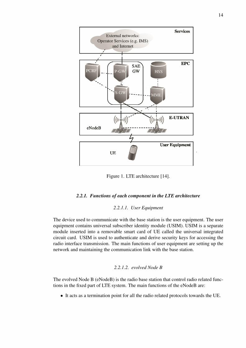
The architecture of the LTE network is depicted in the Figure 1. It is mainly composedof core network (CN) and radio access network (RAN). The CN consist of evolvedpacket core (EPC) and service domain. The RAN is composed of user equipment andevolved universal terrestrial radio access (E-UTRAN).

There are two routers present in CN of EPC. The first router called packet datanetwork gateway (P-GW) router which is used to connect the external services. Thesecond router is divided into service gateway (S-GW) and mobility management en-tity (MME). The S-GW provides data transport service to the eNodeB from the CN.The MME performs the control functions and is connected to the database home sub-scription server (HSS). The S-GW and P-GW are the core elements in the networkarchitecture and termed as system evolution architecture gateways (SAE GW). TheE-UTRAN in RAN is a mesh of evolved NodeB’s (eNodeB) which are connectedeach other using an interface called X2. The user equipment, E-UTRAN and EPCare connected through internet protocol (IP) [14]. Since the network components areconnected through IP, thus LTE supports packet switching unlike circuit switching inprevious generation mobile communication systems.

14

Figure 1. LTE architecture [14].

2.2.1. Functions of each component in the LTE architecture

2.2.1.1. User Equipment

The device used to communicate with the base station is the user equipment. The userequipment contains universal subscriber identity module (USIM). USIM is a separatemodule inserted into a removable smart card of UE called the universal integratedcircuit card. USIM is used to authenticate and derive security keys for accessing theradio interface transmission. The main functions of user equipment are setting up thenetwork and maintaining the communication link with the base station.

2.2.1.2. evolved Node B

The evolved Node B (eNodeB) is the radio base station that control radio related func-tions in the fixed part of LTE system. The main functions of the eNodeB are:

• It acts as a termination point for all the radio related protocols towards the UE.

15

• It is responsible for control plane functions, radio resource management (RRM)(e.g., allocating resources, maintaining quality of service (QOS), and monitoringusage of resources).

• It plays an important role in mobility management (MM). eNodeB performs therequired signal level measurements to handover the UE’s inbetween cells.

2.2.1.3. Mobility Management Entity

Mobility management entity (MME) is control element of EPC. It is used only incontrol plane. The main functions of MME are

• Authentication and security: MME performs the authentication procedure when-ever the user equipment registers for the first time. A detailed authenticationprocedure named ’EPS-AKA’ is presented in [15]. The MME initiates the au-thentication procedure when needed or periodically. The MME also assigns eachUE a temporary identity called global unique temporary identity (GUTI). GUTIreduces the transmission of permanent UE identity (i.e., international mobilesubscriber identity (IMSI)) over the radio interface to protect user equipment’sprivacy.

• Mobility management: The MMEs keep track of the user equipment locationand its service areas. MME requests the appropriate resources to be setup fromthe eNodeB and S-GW for the UE. MME also participates in control signallingfor handover of UE between the eNodeBs and S-GWs.

• Managing profile subscription and service connectivity: Whenever a UE regis-ters to the network, MME automatically sets up a default bearer providing thebasic IP connectivity to UE. Then MME retrieves the subscription profile fromthe home network. The subscription profile details the packet data network con-nections that are needed to be allocated to the user equipment.

2.2.1.4. Packet Data Network Gateway

Packet data network gateway (P-GW) is a router between the evolved packet system(EPS) and external packet data networks. The EPS comprises of EPC, E-UTRANand user equipment. P-GW assigns the IP address to the UE using the dynamic hostconfiguration protocol (DHCP). The user plane traffic between P-GW and externalnetworks is in the form of IP packets. The P-GW also controls the user plane tunneldata delivery in the uplink and downlink of S-GW.

2.2.1.5. Serving Gateway

The main functions of the serving gateway (S-GW) are user plane tunnel managementand switching. A tunnel is created between P-GW and eNodeB when UE is connected

16

to the network. Tunnel management of S-GW refers to swapping the tunnel connectionfrom one eNodeB to another eNodeB during the UE mobility. The S-GW also sets up,clear, or modifies bearers for the UE based on the requests from MME, P-GW, andpolicy and charging resource function (PCRF).

2.2.1.6. Home Subscription Server

Home subscription server (HSS) is the subscription data repository of all permanentusers (subscribers). The subscriber profile is stored in HSS. The subsequent authenti-cation keys derived from permanent user key used for user authentication are stored inauthentication center (AuC) which is a part of the HSS.

2.2.1.7. Services Domain

The service domain offer different kinds of services (e.g., web browsing, voice, anddata streaming) to various subsystems in LTE. There are mainly three categories ofservices offered in the service domain. The offered services in the service domain are

• IP based multimedia services (IMS): The IMS based services are offered in theLTE network with session initiation protocol (SIP). The more details of the IMSarchitecture is defined in [16].

• Non-IMS based operator services (Non-IMS): The architecture for Non-IMSbased services is not defined by the 3GPP. A server can be attached to the net-work via some agreed protocol that is supported by an application in the UE(e.g., video streaming).

• Other services: The other services include (e.g., services offered through inter-net) are not provided by the mobile operator. The architecture depends on theoffered service. The architecture for providing other services is not addressed in3GPP.

2.3. Downlink communication

The RAN of the LTE architecture in the downlink communication uses orthogonalfrequency division multiplexing access (OFDMA). OFDMA is also used in other ra-dio communication systems (e.g., worldwide interoperability for microwave access(WIMAX) [17], digital video broadcasting (DVB) [18]). OFDMA is multi user chan-nel access technique based on the OFDM. The OFDM approach was first proposed byR.W.Chang [19]. The basic principle of OFDM is to divide the available spectrum intoparallel narrowband channels referred as subcarriers and transmit information on theseparallel channels at a reduced signaling rate [20].

17

Figure 2. OFDM transmitter and receiver block diagram [20].

Figure 3. (a) Pulse shape in time domain. (b) Single subcarrier spectrum in frequencydomain. [21].

Figure 4. OFDM transmission [14].

The Figure 2 shows the block diagram of OFDM transmitter and receiver used inRAN of LTE downlink system. At the transmitter in Figure 2, the data bits are firstlymodulated either using quadrature amplitude modulation (QAM) or phase shift keying(PSK) and are then converted to parallel data streams through demultiplexing. Theparallel data streams are mapped to different subcarriers. The shape of a single sub-carrier in time domain and spectrum in frequency domain is shown in Figure 3. LTE

18

comprises maximum of 2048 subcarriers in the available bandwidth with spacing of15 KHz within each other. The placing of subcarriers in an OFDM transmission withspacing of 15 KHZ is shown in Figure 4. The subcarriers are made orthogonal usingfast fourier transform (FFT) technique. The FFT converts the signal from time domainto frequency domain. The parallel data streams which are obtained after modulationare subjected to inverse FFT. The output of IFFT is the sum of signal samples. Cyclicprefix (CP) is added to the IFFT output symbols to avoid inter symbol interference(ISI). The addition of CP refers to prefixing symbols with a copy of the end of thesymbol as shown in Figure 5. CP also helps to preserve the orthogonality betweensubcarriers. The CP added output symbols from IFFT are then converted to analog andtransmitted to the receiver.

Figure 5. Cyclic Prefix [22].

At the receiver, the analog signal is converted back to digital form and CP is re-moved. The digital signal is then subjected to FFT which reverses the effect of IFFTat the transmitter. The output signal is equalized. The main purpose of equalization isto avoid ISI during signal transmission. The equalized symbols are then demodulatedback in to output as bits.

OFDM baseband signal can be represented by:

s(t) =

N�1X

k=0

X(k) ⇤ ej2⇧k�ft, (2.1)

where s(t) is the time domain representation of OFDM signal, N represents the numberof subcarriers, X(k) is the kth subcarrier, �f is the subcarrier spacing and t is time inseconds.

2.4. Uplink communication

The uplink communication in the 3GPP LTE standard [11] occurs from user equipmentto the eNodeB. Single carrier- frequency division multiple access (SC-FDMA) is themodulation technique used in uplink communication. Due to high peak to averagepower ratio (PAPR) caused by OFDM signals in downlink communication of LTE,SC-FDMA is selected for the uplink communication. The block diagram of SC-FDMAtransmitter and receiver is presented in Figure 6.

19

Figure 6. SC-FDMA transmitter and receiver block diagram [22].

At the transmitter, the input data bits are modulated before performing N-point dis-crete fourier transform (DFT). The common modulation schemes used are quadraturephase shift keying (QPSK), binary phase shift keying (BPSK), 16-ary QAM, and 64-QAM. The modulation scheme is chosen, depending on the radio channel. The mod-ulated data symbols are then converted into N parallel data streams. Then N-pointDFT is performed on the parallel streams. DFT converts the time domain modulatedsymbols to frequency domain symbols. The obtained N output frequency domain sym-bols are mapped to M orthogonal subcarriers, where M is an integer multiple of l. Mcan be represented as M=l*Q where Q is the bandwidth expansion factor or the max-imum number of users that can be supported in the system For example, if there are l= 64 output frequency domain symbols and M= 256 orthogonal subcarriers then Q = 4users can be supported. After the subcarrier mapping, the complex frequency domainsymbols are converted back to time domain signals using inverse DFT (IDFT). Cyclicprefix (CP) is then added to time domain signal to avoid inter symbol interference (ISI)similar to downlink communication. CP also helps to maintain the periodicity of thesignal. To maintain the desired spectrum at the receiver pulse shaping is performed atthe transmitter. The pulse shaped signal is converted to analog signal using digital toanalog (D/A) converter. The analog signal is transmitted to the receiver through theradio channel.

At the receiver, the analog signal is converted back to digital form using analog todigital (A/D) converter followed by CP removal. The time domain signal is convertedto frequency domain symbols. The subcarrier demapping is performed. Once the sub-carrier demapping is done the symbols are subjected to frequency domain equalization.The most commonly used equalizer is the minimum mean square error (MMSE) fre-quency domain equalizer. The frequency domain equalized signal is then converted totime domain using IDFT. The output symbols are finally demodulated to data bits.

20

2.5. Challenges for implementing LTE in smart meters

The implementation of LTE in smart meters pose many research challenges. Some ofthe key challenges are:

• Flexible architecture approach: The network architecture should be designedhighly flexible. The devices should have the ability to connect to a aggregationpoint (AP) (e.g., direct and indirect method) or among themselves (e.g., Ad-hoc).The direct and indirect architectures used in smart meters [23] while using LTEare shown in Figure 7. In direct method shown in Figure 7 a), the smart meterhas the broadband access module along with the device and they communicatedirectly with the base station. Relay nodes are used to extend the coverage area.

Figure 7. LTE Architectures for smart metering [23].

In indirect method shown in Figure 7 b), the smart meter communicates with theAP and then AP communicates with the base station. In this thesis for evaluat-ing LTE in smart meters, direct communication architecture is considered. Theaverage load and delay posed by the smart meter traffic when smart meters useLTE is discussed in Section 5.1.3.

• Congestion control: As there would be a major increase in the usage of LTEthe eventuality of congestion may also increase. The feasibility study of thesmart meter traffic without hindering LTE background applications is studied inSection 5.3. The congestion in the LTE traffic when used in smart meters canhappen at:

– Radio network part: As there is increase in the number of UE’s, the usageof same channels by different UE’s can cause collisions.

– EPC network part: The another bottleneck in the network architecture is inthe core devices, which communicate with the radio network access part.

21

The components (e.g., MME, S-GW and P-GW) are responsible for at-tachment of UE’s and will send, and receive traffic simultaneously causingcongestion to the network.

Figure 8. Congestion in LTE network architecture.

• Traffic scheduling: Smart meters connect (or reconnect) to the wireless broad-band network (i.e., LTE) during the exchange of information. The traffic gen-erated by smart meters is generally regarded to be periodic. Hence, the trafficgenerated by the smart meters by connecting and reconnecting for specific in-stances of time is called time controlled traffic. Smart meters are connected onlyfor a specific duration in time controlled operation. The duration of the con-nected intervals can be configured to be different for each smart meter and canbe dynamically adjusted by the network as needed. In scenarios related to criti-cal alarm indication, data from the smart meter should be reported immediatelyand not be queued until the next scheduled connected period. Therefore, withinframework of time controlled operation, the smart meters shall be allowed tosend messages outside its assigned interval and the system should allow for suchunscheduled transactions to be processed.

22

3. SURVEY ON IEEE 802.15.4 STANDARD WIRELESSSENSOR NETWORKS

3.1. Introduction

A wireless sensor network (WSN) is a collection of nodes which have the ability ofactuation, sensing, computing and communication. Sensor nodes in WSN communi-cate through wireless channels in real time providing information to utility and the endusers. There are two types of nodes defined by the IEEE 802.15.4 [12] standard typeWSN. They are full-function device (FFD) and reduced-function device (RFD). FFDis a node which can operate as personal area network (PAN) coordinator, or as an endnode but RFD operates only as end node. Sensor networks have architectures of star,peer to peer, mesh and cluster tree. The star and peer to peer topologies are the mostcommonly used, and are shown in Figure 9.

Figure 9. Star, and Peer to Peer Topology for IEEE 802.15.4 type WSN [12].

Communication between the nodes in a star topology is established using singlecentral controller known as personal area network (PAN) coordinator. All the devicesconnected in the network will use unique address or an extended address which is as-signed by the PAN coordinator. Other nodes in the network can communicate throughthe PAN coordinator. In peer to peer network topology, any node can communicatewith any other node as long as they are in range of one another. An example of peer topeer communication topology is cluster tree network topology. In cluster tree networktopology all the devices are FFDs. An RFD can connect to a cluster tree network as aleaf node at the end of a branch because RFDs do not allow other devices to associate.

In IEEE 802.15.4 [12] standard, the architecture of sensor node is defined in termsof blocks called layers. Each layer is part of the IEEE 802.15.4 [12] standard. Theyare physical, MAC and upper layers. In this chapter, the functionalities of the physicaland MAC layer are studied with respect to the standard 802.15.4 [12]. The physicallayer consist of radio frequency (RF) transceiver with low level control mechanism andprovides mainly two kinds of services, PHY data and management service at serviceaccess points (SAPs). The physical layer is connected to MAC layer using the physicaldata service access point (PD-SAP) and physical layer management entity (PLME)

23

SAP. The MAC also has MAC data and MAC management service. The MAC layer isconnected similarly to upper layers using MAC sublayer management entity (MLME)and MAC common part sublayer (MCPS) SAP.

3.2. Physical layer (PHY)

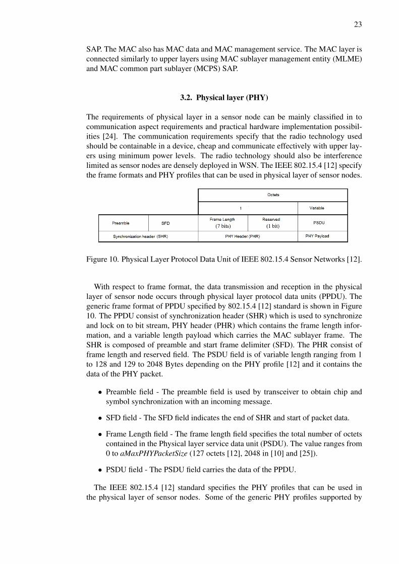
The requirements of physical layer in a sensor node can be mainly classified in tocommunication aspect requirements and practical hardware implementation possibil-ities [24]. The communication requirements specify that the radio technology usedshould be containable in a device, cheap and communicate effectively with upper lay-ers using minimum power levels. The radio technology should also be interferencelimited as sensor nodes are densely deployed in WSN. The IEEE 802.15.4 [12] specifythe frame formats and PHY profiles that can be used in physical layer of sensor nodes.

Figure 10. Physical Layer Protocol Data Unit of IEEE 802.15.4 Sensor Networks [12].

With respect to frame format, the data transmission and reception in the physicallayer of sensor node occurs through physical layer protocol data units (PPDU). Thegeneric frame format of PPDU specified by 802.15.4 [12] standard is shown in Figure10. The PPDU consist of synchronization header (SHR) which is used to synchronizeand lock on to bit stream, PHY header (PHR) which contains the frame length infor-mation, and a variable length payload which carries the MAC sublayer frame. TheSHR is composed of preamble and start frame delimiter (SFD). The PHR consist offrame length and reserved field. The PSDU field is of variable length ranging from 1to 128 and 129 to 2048 Bytes depending on the PHY profile [12] and it contains thedata of the PHY packet.

• Preamble field - The preamble field is used by transceiver to obtain chip andsymbol synchronization with an incoming message.

• SFD field - The SFD field indicates the end of SHR and start of packet data.

• Frame Length field - The frame length field specifies the total number of octetscontained in the Physical layer service data unit (PSDU). The value ranges from0 to aMaxPHYPacketSize (127 octets [12], 2048 in [10] and [25]).

• PSDU field - The PSDU field carries the data of the PPDU.

The IEEE 802.15.4 [12] standard specifies the PHY profiles that can be used inthe physical layer of sensor nodes. Some of the generic PHY profiles supported by

24

IEEE 802.15.4 [12] standard are offset phase shift keying (O-QPSK), binary phaseshift keying (BPSK), and amplitude shift keying (ASK). The PHY profiles specificto 802.15.4k [10] LECIM standard are direct sequence spread spectrum (DSSS) andfrequency shift keying (FSK). Different PHY profiles result in different bit rate andsymbol rate performances. The different PHY alternative profiles with their respectivebit rate and symbol rates are shown in Table 2.

Table 2. Data rates and bit rates in PHY alternatives of 802.15.4 [12] standardPHY Profile Frequency Band Bit Rate Symbol RateModulation (MHz) (Kb/s) (Ksymbol/s)BPSK 902-908 40 40ASK 902-908 250 50O-QPSK 902-908 250 62.5FSK 917 -923.5 12.5 12.5CSS 2400-2483.5 250 166.6O-QPSK 2450 DSSS 250 62.5

Smart metering devices are mainly characterised by large path loss, minimal infras-tructure requirements, and low energy. These requirements must be satisfied whileconsidering the PHY profile. The generic requirements for choosing PHY profile aredata rate, bandwidth efficiency, error performance and design complexity with less in-terference. In general, IEEE 802.15.4 [12] standard supports BPSK, OQPSK, ASK,and CSS PHY profiles. In this thesis, we focus on low energy critical infrastructuremonitoring (LECIM) network application (i.e., smart metering). DSSS and FSK PHYprofiles are mainly designed for LECIM applications (e.g., smart metering). The DSSSPHY profile data rate is band and region specific. DSSS PHY uses different frequencybands in different countries [10]. The DSSS PHY profile uses either BPSK or OQPSKmodulation depending the phyLECIMDSSSPPDUModulation [10]. The FSK PHYprofile uses narrow bandwidth with low data rate devices to enable high sensitivitiesfor reduction in the possibility of collisions. The performance of the chosen PHY pro-file transmission decides the signal level, and the modulation scheme (i.e.,constellationmapping and encoding).

3.3. 802.15.4 MAC layer Family

Introduction

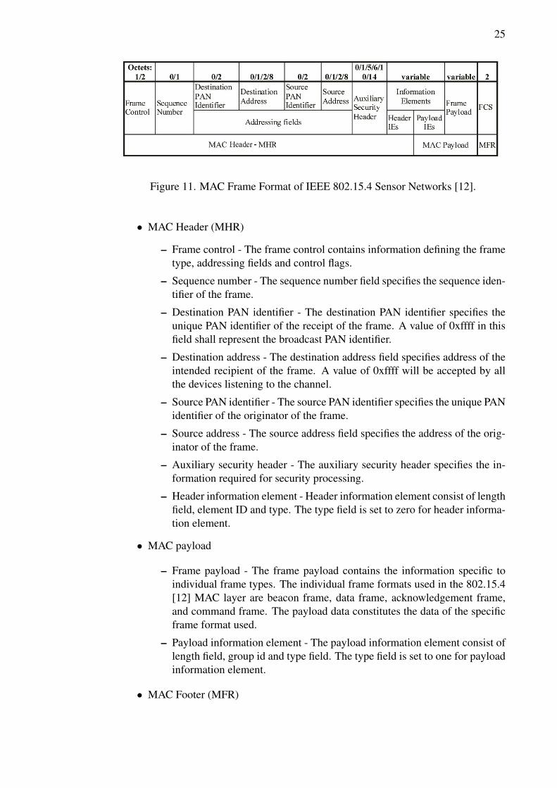
The layer above the PHY is MAC sublayer. The generic requirements of MAC layerare framing, medium access, reliability, flow control, and error control. The mainfunctions of the MAC layer specified by IEEE 802.15.4 [12] are generating networkbeacons if the node is a coordinator, synchronizing to the network beacons, support-ing PAN association and disassociation, device security and employing carrier sensemultiple access - collision avoidance (CSMA-CA) mechanism for channel access. Thegeneric frame format in MAC layer is shown in Figure 11 along with the descriptionof the fields.

25

Figure 11. MAC Frame Format of IEEE 802.15.4 Sensor Networks [12].

• MAC Header (MHR)

– Frame control - The frame control contains information defining the frametype, addressing fields and control flags.

– Sequence number - The sequence number field specifies the sequence iden-tifier of the frame.

– Destination PAN identifier - The destination PAN identifier specifies theunique PAN identifier of the receipt of the frame. A value of 0xffff in thisfield shall represent the broadcast PAN identifier.

– Destination address - The destination address field specifies address of theintended recipient of the frame. A value of 0xffff will be accepted by allthe devices listening to the channel.

– Source PAN identifier - The source PAN identifier specifies the unique PANidentifier of the originator of the frame.

– Source address - The source address field specifies the address of the orig-inator of the frame.

– Auxiliary security header - The auxiliary security header specifies the in-formation required for security processing.

– Header information element - Header information element consist of lengthfield, element ID and type. The type field is set to zero for header informa-tion element.

• MAC payload

– Frame payload - The frame payload contains the information specific toindividual frame types. The individual frame formats used in the 802.15.4[12] MAC layer are beacon frame, data frame, acknowledgement frame,and command frame. The payload data constitutes the data of the specificframe format used.

– Payload information element - The payload information element consist oflength field, group id and type field. The type field is set to one for payloadinformation element.

• MAC Footer (MFR)

26

– FCS - The frame check sequence (FCS) field contains the 16-bit ITU-Tcyclic redundancy check (CRC). The FCS is calculated for both MHR andMAC payload. The evaluation of CRC code is detailed in Section 4.1.1.

The IEEE 802.15.4 MAC supports two modes of operation. They are beacon-enabled mode and nonbeacon-enabled mode. PANs that wish to use the superframestructure are referred to beacon-enabled PANs otherwise called as nonbeacon-enabledPANs. The frame format of the superframe structure is defined by the PAN coordinator.

3.3.1. Superframe structure

The structure of superframe is shown in Figure 12. The superframe structure consist ofbeacon, active and optional inactive portions. The active portion consist of contentionaccess period (CAP) and optional contention free period (CFP). In CFP the node mayrequest the PAN coordinator to allocate guaranteed time slots (GTS). In the inactiveperiod coordinator can enter into sleep mode.

Figure 12. Superframe Structure of IEEE 802.15.4 Sensor Networks [12].

The structure of the superframe is characterized by beacon interval (BI) and super-frame duration (SD). The BI specifies the time between two consecutive beacons. TheSD corresponds to the active period in the superframe structure. The BI and SD aredefined by

BI = aBaseSuperframeDuration ⇤ 2BO (3.1)SD = aBaseSuperframeDuration ⇤ 2SO

where beacon order (BO) and superframe order (SO) are macBeacondOrder andmacSuperframeOrder respectively. In a beacon enabled PAN, the macBeaconOrderand macSuperframeOrder ranges from 0 to 14. If both macBeacondOrder and macSu-perframeOrder equals to 15, coordinator will not transmit beacon frames, and hencereferred as nonbeacon enabled PANs.

3.3.2. CSMA-CA algorithm

Sensor nodes use CSMA-CA algorithm for accessing the channel. The CSMA-CA al-gorithm is used during the CAP of the superframe structure before the transmission of

27

data or MAC command frames. During the transmission of beacon frames, acknowl-edgement frames and data, CSMA-CA is not employed.

If beacon enabled mode is used by PAN, the CSMA-CA algorithm is slotted i.e., thebackoff period boundaries of every device in the PAN are aligned with the superframeboundaries of the PAN coordinator. In slotted CSMA-CA, node that transmits dataframes during the CAP shall first locate the boundary of the next backoff period. Ifnon-beacon enabled mode is used or a beacon cannot be located in a beacon enablednetwork, unslotted CSMA-CA algorithm is used. In unslotted CSMA-CA, the backoffperiods of one device are not synchronized with any other device backoff period in thePAN. But, both slotted and unslotted CSMA-CA algorithms use units of time calledbackoff periods, which is aUnitBackoffPeriod equal to 20 symbols.

There are three main variables used by CSMA-CA algorithm to update for everytransmission attempt. They are 1) Number of backoffs (NB), 2) Contention window(CW), and 3) Backoff exponent (BE). NB is the number of times CSMA-CA algorithmwas required to backoff. CW is the contention window length defining the number ofbackoff periods required for the channel to be clear before transmission. CW is usedonly in slotted CSMA-CA. BE is the number of backoff periods required for a deviceto wait before attempting to assess the channel. BE enables the computation of backoffdelay.

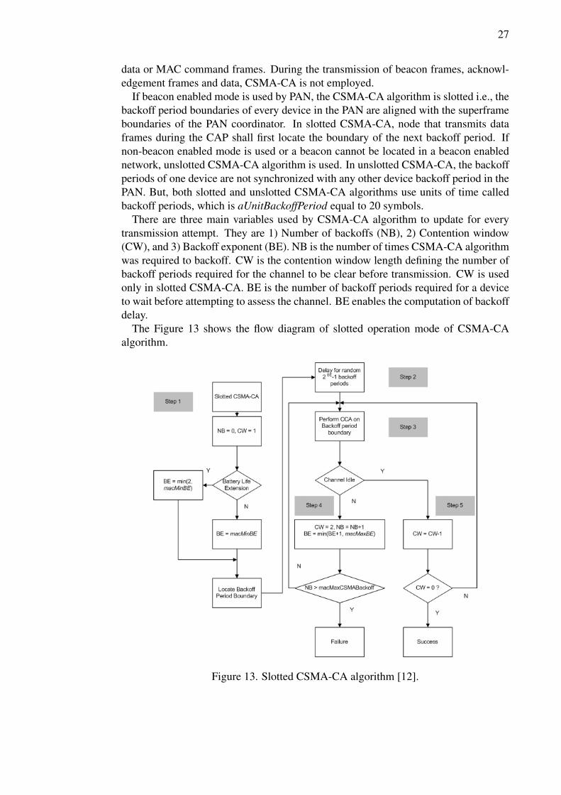
The Figure 13 shows the flow diagram of slotted operation mode of CSMA-CAalgorithm.

Figure 13. Slotted CSMA-CA algorithm [12].

28

The slotted CSMA-CA is carried out in the following steps:

• Step 1: NB, BE, and CW variables are initialized. The boundary of the nextbackoff period is located. The value of BE is decided by the battery life extension(BLE). If BLE is set to zero then BE is initialized to macMinBE. If BLE is set toone then BE is initialized to min(2,macMinBE).

• Step 2: A Random delay of 2BE � 1 backoff periods is introduced for each nodein the sensor network.

• Step 3: After the random backoff delay, the slotted CSMA-CA shall request thePHY to perform clear channel assessment (CCA). CCA is the ability of the PHYto analyze whether the channel is free for transmission.

• Step 4: If the channel is busy, the MAC sublayer shall increment both NB andBE by a value 1. The algorithm ensures that BE cannot be more than mac-MaxBE with NB not more than macMaxCSMABackoff. If NB is more than themacMaxCSMABackoff, CSMA-CA algorithm will terminate with channel accessfailure status.

• Step 5: If the channel assessed is found to be idle, the MAC sublayer wouldcheck for the expiration of CW before transmission. If CW is not equal to zeroCSMA-CA algorithm returns to CW=CW-1. If it is equal to zero the MACsublayer shall begin the transmission on the boundary of the next backoff period.

The Figure 14 shows the unslotted operation mode of CSMA-CA algorithm.

Figure 14. Unslotted CSMA-CA algorithm [12].

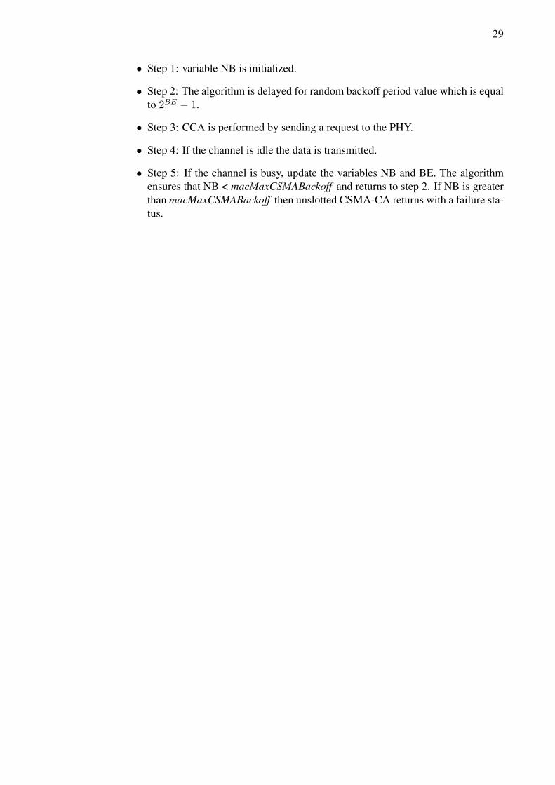
The unslotted CSMA-CA algorithm follows the steps:

29

• Step 1: variable NB is initialized.

• Step 2: The algorithm is delayed for random backoff period value which is equalto 2

BE � 1.

• Step 3: CCA is performed by sending a request to the PHY.

• Step 4: If the channel is idle the data is transmitted.

• Step 5: If the channel is busy, update the variables NB and BE. The algorithmensures that NB < macMaxCSMABackoff and returns to step 2. If NB is greaterthan macMaxCSMABackoff then unslotted CSMA-CA returns with a failure sta-tus.

30

4. ERROR CONTROL ALGORITHMS

4.1. Introduction

In this thesis we wish to study the feasibility of long range IEEE 802.15.4k [10] de-vices in smart meters. The long range WSN devices suffers from higher signal atten-uation and increased channel coherence time. Due to higher channel coherence timeand attenuation the bit error rate (BER) and PER is also increased. This chapter pro-vides the background to understand the underlying mechanisms used to overcome thechannel pathloss and propagation effects in WSN devices. The mechanisms are knownas error control or mitigation algorithms. Error control algorithms are used to detectand correct the transmission errors at the receiver. Error control algorithms [26] arebroadly classified in to forward error correction (FEC) and automatic repeat request(ARQ). FEC [27] scheme uses error correcting code to add redundant bits to the orig-inal message. When the receiver detects an error in the received bits, it attempts todetermine the error locations and corrects the errors using checksum. If the exact lo-cations of the errors are determined the received bits will be correctly decoded. If thereceiver fails to determine the exact location of errors, the received bits will be de-coded incorrectly. In ARQ [27] system, a code with good error detecting capability ischosen. At the receiver the syndrome vector of the received codeword is computed.The syndrome vector is obtained from the parity check matrix. The parity check ma-trix is matrix of redundant bits which are chosen to be added to the original messageby transmitter. If the syndrome vector is zero the received codeword is assumed tobe error free. The receiver notifies the transmitter via a return channel, that the trans-mitted codeword has been successfully received. If the syndrome vector is not zero,errors are detected in received codeword. Then the transmitter is instructed, through areturn channel, to retransmit the same codeword. Retransmission is used to receive thecodeword successfully.

There are three kinds of ARQ [27]. They are

• Stop and wait: In stop and wait scheme, transmitter sends a codeword to thereceiver and waits for an acknowledgement (ACK) from the receiver. A positiveACK from the receiver signals that the codeword has been successfully received(i.e.,no errors are detected). A negative ACK from the receiver indicates thatreceived vector has been detected in error. The transmitter resends the codeword.Retransmissions occur until positive ACK is received by the transmitter.

• Go back N: In go back N scheme codewords are transmitted continuously. Thetransmitter does not wait for an ACK after sending the codeword. When thereis a negative ACK for the Nth codeword. The transmitter backs up to the code-word that was negatively acknowledged and resend that codeword and the N-1succeeding codewords.

• Selective repeat: In selective repeat codewords are transmitted continuously. Butthe retransmission takes only to the negatively acknowledged codewords.

Hybrid ARQ (H-ARQ) is essentially a combination of FEC and ARQ system inan optimal manner [27]. The function of FEC scheme is to reduce the frequency of

31

retransmission by correcting the error patterns. ARQ is used for retransmitting thecorrupt codeword. The H-ARQ scheme combines both. The H-ARQ schemes [28] arefurther classified into

• Type I, chase combining (CC) [26] - When receiver requests for retransmission,the retransmissions consist of same set of coded bits as the original transmission.In other words the coding technique used in the original transmission will not bealtered even for retransmission. In Type I H-ARQ systems, the receiver com-bines each received codeword with any of the previous transmissions of samecodeword to make decoding easy.

• Type II, incremental redundancy (IR) [29] - The retransmissions are not iden-tical to the original transmission. The coded redundant bits are different thanthe previous transmission. Multiple sets of redundant bits are generated by thetransmitter for the same information bits.

• Type III [26] - The type III scheme is similar to incremental redundancy but usespuncturing techniques to create a set of bits. In puncturing some of the paritybits are removed to improve the efficiency of coding. The removed parity bitsare known at the receiver.

4.1.1. Error detection

Error detection is performed in ARQ mechanisms using error detecting codes. Someof the examples of error detecting codes are

• Cyclic redundancy check (CRC) codes. In CRC codes, a group of error controlbits are appended at the end of the original message. The error control bits areobtained as the result of polynomial division of the original message using thegenerator polynomial. If the remainder of the polynomial division is zero orsome other known preset value at the receiver then the original data message isnot corrupted, if not the receiver requests for retransmission.

Figure 15. Polynomial Division at transmitter [30].

32

An example of CRC coding is shown in Figure 15, the dataword "1001" is trans-mitted. The control bits "110" are obtained by division of the original data messagewith the predefined generator polynomial "1011". The codeword transmitted is a com-bination of original message and remainder of the polynomial division. The polyno-mial division using the same generator polynomial is evaluated at the receiver with thetransmitted codeword as shown in Figure 16.

Figure 16. Polynomial Division at Receiver [30].

If the syndrome is zero, the codeword received is not corrupted due to the com-munication channel. If the reminder is not zero, the receiver discards the receivedcodeword and requests for retransmission. Even if the remainder or syndrome is equalto zero there can be a possibility of error in the received codeword, which is termedas undetected error. Undetected error is used as a performance criteria for evaluatingCRC codes. In this thesis to evaluate the appropriate CRC size in MAC frame of IEEE802.15.4k [10], undetected error probability is used. The section 6.2 details the analy-sis of undetected error probabilities for 8, 16, 24, and 32 bit generator polynomials ofCRC codes.

4.1.2. Error correction

Error correction is performed in FEC using error correcting codes (ECC). ECC are usedto correct the errors. ECC are classified mainly into block and convolutional codes.The difference between block and convolutional codes, is the calculation of checksumvalue which is attached along with the data for protection. In block codes the parity orcheck bits are calculated only from the information bits but in convolutional codes theparity bits are obtained using the previous information blocks as in Figure 17.

33

Figure 17. Classification of Error Correction Codes.

4.1.2.1. Block Codes

In block codes, the encoder divides the information sequence into message blocks ofk information bits (i.e., symbols) each. Each k information bit or symbol block istreated as the original message. Error correction bits are appended for every blockof this message. Some of the examples of block codes are reed solomon (RS) codes,Hamming codes, Hadamard codes, golay codes and reed-muller codes.

4.1.2.2. Reed Solomon codes

Reed Solomon codes are systematic linear block codes developed by Irving Reed andGustave Solomon [31]. It is called as systematic code, because the original messageblock codeword is left intact even after encoding and decoding.

RS code is defined as (n,k) code, where n represents the block length in symbols andk represent the message length in symbols. Symbols can contain m bits. The encodertakes k symbols where each symbol can contain a maximum of 8 binary bits. Themessage symbols k are represented in Galois Field (GF) polynomial. The messagepolynomial is multiplied with x

n�k to allow space for the parity symbols. The multi-plied message polynomial is divided using a code generator polynomial derived fromthe GF. The remainder is appended to form the transmitted message symbols.

The block length n for a given code is given by:

n 2

m � 1 (4.1)

34

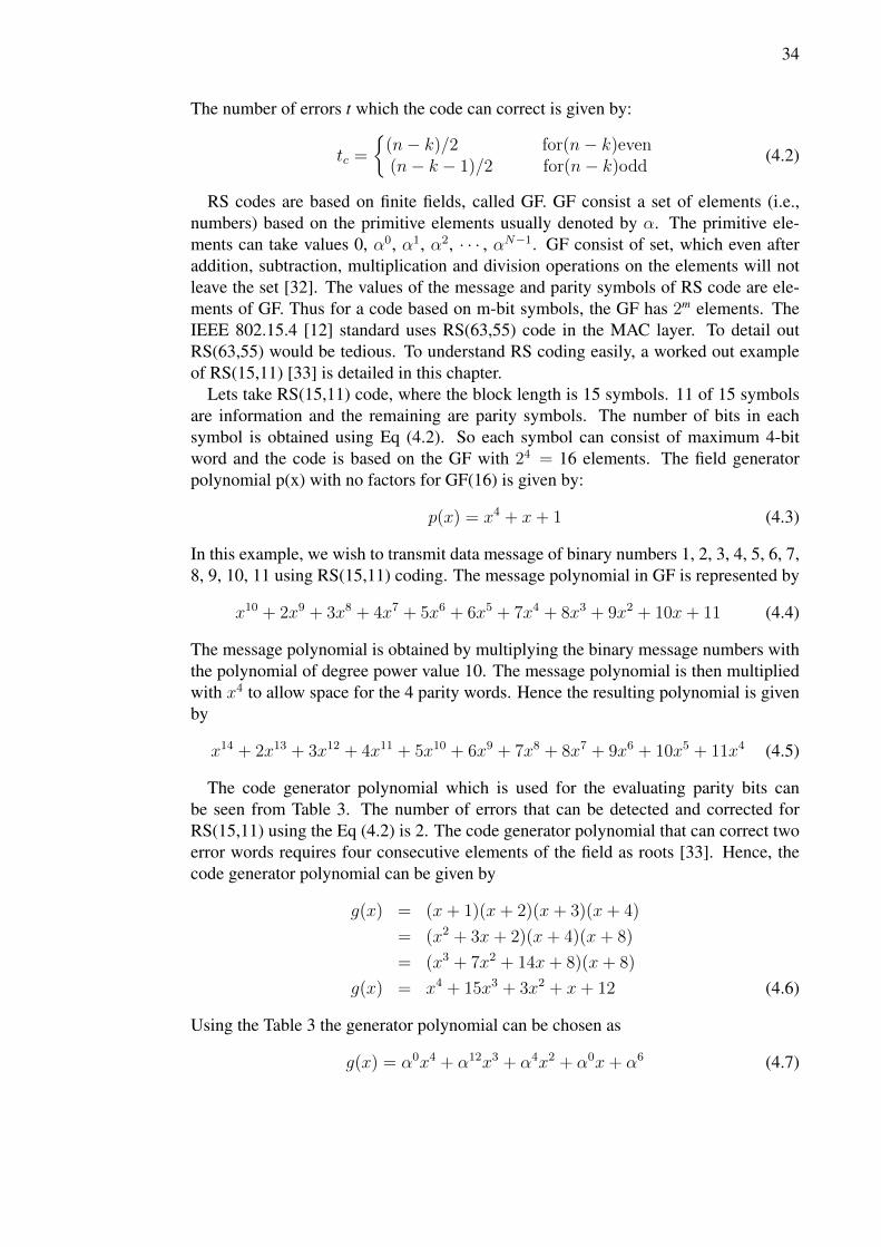
The number of errors t which the code can correct is given by:

tc =

⇢(n� k)/2 for(n� k)even

(n� k � 1)/2 for(n� k)odd

(4.2)

RS codes are based on finite fields, called GF. GF consist a set of elements (i.e.,numbers) based on the primitive elements usually denoted by ↵. The primitive ele-ments can take values 0, ↵0, ↵1, ↵2, · · · , ↵N�1. GF consist of set, which even afteraddition, subtraction, multiplication and division operations on the elements will notleave the set [32]. The values of the message and parity symbols of RS code are ele-ments of GF. Thus for a code based on m-bit symbols, the GF has 2

m elements. TheIEEE 802.15.4 [12] standard uses RS(63,55) code in the MAC layer. To detail outRS(63,55) would be tedious. To understand RS coding easily, a worked out exampleof RS(15,11) [33] is detailed in this chapter.

Lets take RS(15,11) code, where the block length is 15 symbols. 11 of 15 symbolsare information and the remaining are parity symbols. The number of bits in eachsymbol is obtained using Eq (4.2). So each symbol can consist of maximum 4-bitword and the code is based on the GF with 2

4= 16 elements. The field generator

polynomial p(x) with no factors for GF(16) is given by:

p(x) = x

4+ x+ 1 (4.3)

In this example, we wish to transmit data message of binary numbers 1, 2, 3, 4, 5, 6, 7,8, 9, 10, 11 using RS(15,11) coding. The message polynomial in GF is represented by

x

10+ 2x

9+ 3x

8+ 4x

7+ 5x

6+ 6x

5+ 7x

4+ 8x

3+ 9x

2+ 10x+ 11 (4.4)

The message polynomial is obtained by multiplying the binary message numbers withthe polynomial of degree power value 10. The message polynomial is then multipliedwith x

4 to allow space for the 4 parity words. Hence the resulting polynomial is givenby

x

14+ 2x

13+ 3x

12+ 4x

11+ 5x

10+ 6x

9+ 7x

8+ 8x

7+ 9x

6+ 10x

5+ 11x

4 (4.5)

The code generator polynomial which is used for the evaluating parity bits canbe seen from Table 3. The number of errors that can be detected and corrected forRS(15,11) using the Eq (4.2) is 2. The code generator polynomial that can correct twoerror words requires four consecutive elements of the field as roots [33]. Hence, thecode generator polynomial can be given by

g(x) = (x+ 1)(x+ 2)(x+ 3)(x+ 4)

= (x

2+ 3x+ 2)(x+ 4)(x+ 8)

= (x

3+ 7x

2+ 14x+ 8)(x+ 8)

g(x) = x

4+ 15x

3+ 3x

2+ x+ 12 (4.6)

Using the Table 3 the generator polynomial can be chosen as

g(x) = ↵

0x

4+ ↵

12x

3+ ↵

4x

2+ ↵

0x+ ↵

6 (4.7)

35

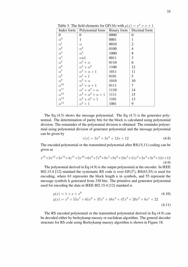
Table 3. The field elements for GF(16) with p(x) = x

4+ x+ 1

Index form Polynomial form Binary form Decimal form0 0 0000 0↵

0 1 0001 1↵

1↵ 0010 2

↵

2↵

2 0100 4↵

3↵

3 1000 8↵

4↵+1 0011 3

↵

5↵

2+ ↵ 0110 6

↵

6↵

3+ ↵

2 1100 12↵

7↵

3+ ↵ + 1 1011 11

↵

8↵

2+ 1 0101 5

↵

9↵

3+ ↵ 1010 10

↵

10↵

2+ ↵ + 1 0111 7

↵

11↵

3+ ↵

2+ ↵ 1110 14

↵

12↵

3+ ↵

2+ ↵ + 1 1111 15

↵

13↵

3+ ↵

2+ 1 1101 13

↵

14↵

3+ 1 1001 9

The Eq (4.5) shows the message polynomial. The Eq (4.7) is the generator poly-nomial. The determination of parity bits for the block is calculated using polynomialdivision. The remainder of the polynomial division is obtained. The reminder polyno-mial using polynomial division of generator polynomial and the message polynomialcan be given by

r(x) = 3x

3+ 3x

2+ 12x+ 12 (4.8)

The encoded polynomial or the transmitted polynomial after RS(15,11) coding can begiven as

x

14+2x

13+3x

12+4x

11+5x

10+6x

9+7x

8+8x

7+9x

6+10x

5+11x

4+3x

3+3x

2+12x+12

(4.9)The polynomial derived in Eq (4.9) is the output polynomial at the encoder. In IEEE

802.15.4 [12] standard the systematic RS code is over GF(26), RS(63,55) is used forencoding, where 63 represents the block length n in symbols, and 55 represent themessage symbols k generated from 330 bits. The primitive and generator polynomialused for encoding the data in IEEE 802.15.4 [12] standard is

p(x) = 1 + x+ x

6 (4.10)g(x) = x

8+ 55x

7+ 61x

6+ 37x

5+ 48x

4+ 47x

3+ 20x

2+ 6x

1+ 22

(4.11)

The RS encoded polynomial or the transmitted polynomial derived in Eq (4.9) canbe decoded either by berleykamp massey or euclidean algorithm. The general decoderstructure for RS code using Berleykamp massey algorithm is shown in Figure 18.

36

Figure 18. Reed Solomon decoder [33].

In decoding of the RS encoded codeword, the first step is the evaluation of syndromecomponents. Syndrome calculation is similar to parity evaluation and is calculated for2t syndrome components (i.e., s0, s1, · · · , s3 for RS(15,11) code). If the remainder ofthe polynomial division is equal to zero for all syndrome components, it can be inferredthat the transmitted polynomial shown in Eq (4.9) was not subjected to any errors.Otherwise the error location polynomial is derived using the syndrome polynomialand error evaluation polynomial. The error location location L(x) and syndrome s(x)polynomials are related by

L(x)s(x) = W (x)modX

2t, (4.12)

Where syndrome polynomial s(x), error location polynomial L(x), and error evaluationpolynomials W(x) are given by

s(x) = s0 + s1x1+ s2x

2+ · · ·+ s2t�1x

2t�1 (4.13)L(x) = 1 + L1x+ L2x

2+ L3x

3+ · · ·+ Lex

e

W (x) = 1 +W1x+W2x2+W3x

3+ . . .+We�1x

e�1,

where e represent the number of errors. The Berleykamp Massey algorithm [34] isused for evaluation of error location and syndrome polynomial. The error locations areobtained using chien search algorithm [35]. The error magnitudes are evaluated usingForney algorithm [36]. The error correction is done by adding the corrupted symbol tocorrect the error.

4.1.2.3. Convolution codes

Convolution codes are developed by Elias [37]. In block codes k information symbolsare encoded in to n information symbols. But in convolution codes, encoding schemetakes in to consideration of the current and previously sent messages. In order toutilize preceding messages convolution codes use memory element at the encoder. Thedecoding algorithm of the convolution codes is done using Viterbi algorithm [30].

37

The generalized convolution encoder consist of input shift register that outputs n0

binary digits for every k0 information digits presented at its input. As a block of k0digits enter the register, the n0 modulo-2 adders feed the output register with the n0

digits and these are shifted out. The code rate is given by Rc = k0/n0. It is visible thatthe encoding of n0 digits not only depend on k0 but also the previous (N � 1)k0 digitswhich constitutes the memory � = (N � 1)k0 of the encoder. Hence the convolutioncode is represented as (n0, k0, N) code. The parameter N denotes the constraint length.To understand the encoding scheme, N submatrices G1, G2, . . ., GN containing k0

rows and n0 columns. The submatrix Gi describes the connection between the k0 inputregister and n0 output register. In IEEE 802.15.4 [12] standard PPDU is encoded usingconvolution coding. The code rate is Rc = 1/2 which means that k0 = 1 and n0 = 2.

g0 = 010 (4.14)g1 = 101

Figure 19. PPDU convolutional encoder [12].

The Figure 19 shows the convolution encoding scheme performed at PHY layer. Thetransmitted PPDU is encoded using the convolutional encoder with the generator poly-nomial in Eq (4.15). The generator polynomials represents the connection of memoryelements with the modulo-2 adders.

4.1.3. Sensor networks

Sensor networks (IEEE 802.15.4 [10]) can use three kinds of mechanisms for errorrecovery [38]. They are ARQ, error correction coding (ECC), and HARQ. The basicARQ protocols, stop-n-wait, goback-N, and selective repeat are also used for higher re-liability [27]. ECC uses ARQ with coding for the retransmitted packet during adversechannel conditions. Different coding schemes can be used for sensor networks to over-come errors in wireless communication channels. Some of them include BCH [39],RS codes [40], turbo codes [41]. The error correction capability is obtained in WSNdevices at the expense of a high redundancy in the transmitted data and complex de-coding circuitry [41].

38

The IEEE 802.15.4k [10] standard MAC layer fragmentation simulations are per-formed in Section 6.3. The simulations use ARQ with CRC coding to analyze the frag-ment and FCS values. The reason to chose ARQ based error mitigation algorithm is toreduce the complexity of the decoding compared to FEC algorithm. The paper [42] dis-cusses the competitiveness of FEC and ARQ algorithm using BCH block coding. It canbe inferred from the conclusions of the paper [42] that ARQ outperforms the capabili-ties of FEC. Hence ARQ is chosen as the error mitigation algorithm in this thesis. ARQscheme uses an error detection code to determine the corrupted fragment or packet andthen retransmit. Here, in the simulations we chose CRC code as error detection codebecause they do not have built in error correction capability unlike any other blockor convolutional coding and are much easy to implement. The WSN devices are alsopower limited and produce low signal to noise ratio. To overcome these challenges bi-nary linear block codes (i.e., CRC codes) are chosen and are found to be efficient [27]compared to RS, BCH codes in this scenarios. Hence the proposed algorithm in Sec-tion 6.3.0.1 uses ARQ based CRC coding to evaluate the undetected error probabilitiesfor each fragment and packet.

39

5. SIMULATION RESULTS

5.1. LTE Model

In this chapter, the simulation results of smart meters using LTE and WSN in suburbanenvironments are discussed. The simulations are performed in Opnet modeler v16.1[43]. The simulations show the load and delay profile of smart meter traffic whenimplemented using LTE. The results show that LTE and WSN can handle smart metertraffic requirements [9] without hindering their respective background applications.

5.1.1. Topology description

The LTE simulations are done in suburban environment. The suburb of Jääli, inKiminki is chosen as a model for implementing LTE in smart meters. The suburbanenvironment is chosen, as it largely consist of houses instead of apartment buildings orrow houses resulting in lower density of remote terminal units (RTU). The total sub-urb is divided in to clusters as shown in Figure 20. Each cluster dimension roughlyabout 150m*150m and constitute around 25 smart meters. There are about 30 of suchclusters in the area that is contained in space 2.5 km*1.5 km. Therefore the expectednumber of AMR RTUs to be 750 units in the whole area. The RTUs are randomlyplaced inside every cluster at the start of the each simulation run. The purpose of therandom placement is to let the AMR units to be placed in various locations, not dictatedby municipal planning as is usually in real environments. For simulation purpose, it isassumed that each house has one RTU that is connected with an LTE-network eNodeB.

Figure 20. LTE simulation topology.

It is envisioned that a single LTE cell, using 1805-1880 MHz frequency band, couldentirely cover Jääli area. The assumption is that all of the RTUs are serviced by a

40

single LTE carrier. The RF environment chosen will be mostly free space, light trees,and houses being the main obstructions for communications. The simulations are per-formed independently using LTE. The propagation model for LTE is detailed in Section5.1.2

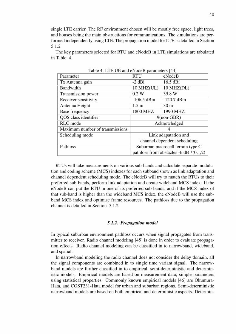
The key parameters selected for RTU and eNodeB in LTE simulations are tabulatedin Table 4.

Table 4. LTE UE and eNodeB parameters [44]Parameter RTU eNodeBTx Antenna gain -2 dBi 16.5 dBiBandwidth 10 MHZ(UL) 10 MHZ(DL)Transmission power 0.2 W 39.8 WReceiver sensitivity -106.5 dBm -120.7 dBmAntenna Height 1.5 m 30 mBase frequency 1800 MHZ 1990 MHZQOS class identifier 9(non-GBR)RLC mode AcknowledgedMaximum number of transmissions 4Scheduling mode Link adapatation and

channel dependent schedulingPathloss Suburban macrocell terrain type C

pathloss from obstacles -6 dB *(0,1,2)

RTUs will take measurements on various sub-bands and calculate separate modula-tion and coding scheme (MCS) indexes for each subband shown as link adaptation andchannel dependent scheduling mode. The eNodeB will try to match the RTUs to theirpreferred sub-bands, perform link adaptation and create wideband MCS index. If theeNodeB can put the RTU in one of its preferred sub-bands, and if the MCS index ofthat sub-band is higher than the wideband MCS index, the eNodeB will use the sub-band MCS index and optimise frame resources. The pathloss due to the propagationchannel is detailed in Section 5.1.2.

5.1.2. Propagation model

In typical suburban environment pathloss occurs when signal propagates from trans-mitter to receiver. Radio channel modeling [45] is done in order to evaluate propaga-tion effects. Radio channel modeling can be classified in to narrowband, wideband,and spatial.

In narrowband modeling the radio channel does not consider the delay domain, allthe signal components are combined in to single time variant signal. The narrow-band models are further classified in to empirical, semi-deterministic and determin-istic models. Empirical models are based on measurement data, simple parametersusing statistical properties. Commonly known empirical models [46] are Okumura-Hata, and COST231-Hata model for urban and suburban regions. Semi-deterministicnarrowband models are based on both empirical and deterministic aspects. Determin-

41

istic models are site specific and they require enormous amount of geometry and ge-ographical site information e.g., Allsebrrok-parsons, Walfish-Bertoni, and COST231-Walfish/Ikegami models [45].

In wideband modeling each received signal component is separated with respect todelay domain. Each delayed domain constitute single propagation path. The receivedsignal is the sum of the delayed paths. In wideband modeling delay spread, and coher-ence bandwidth, coherence time are taken in to consideration.

In spatial channel modeling there are more than one transmit and receive antennas.The channel is analyzed for multiple input multiple output (MIMO). The propagationchannel model is a matrix with nt transmit and rm receive pairs [45].

The channel model for smart meters when deployed in suburban environment is acombination of outdoor propagation loss, indoor propagation loss, and building pene-tration loss [47]. While considering indoor propagation, the loss can be due to differentkinds of obstacles. The respective losses incurred due to common obstructions duringindoor propagation can be found from [48]. To model all the incurred losses due toindoor and outdoor propagation can be complicated. So in simulation the modelingof outdoor and indoor propagation is done using predefined channel model [49] andlosses caused by external walls during the signal propagation with 6 dB [50] for eachwall. The simulations are performed in such a way that radio wave signal can enter amaximum of 3 walls before reaching the end device.

5.1.2.1. LTE propagation model

LTE uses simultaneous data transmission through low rate parallel orthogonal chan-nels. The advantage of using LTE is that all the orthogonal channels face narrow bandfading i.e., frequency variable channel appears flat over the narrow band of OFDMsubcarrier, eliminating the need of complex equalisation. Hence narrow band radiochannel modeling can be used for evaluating the channel propagation effects. Onesuch narrowband empirical model that can be used for evaluating suburban scenariosis suburban macrocell model developed by 3GPP [51] which uses modified COST231HATA model [49].

The simulator chosen is opnet modeler v16.0, LTE specialized model. Opnet mod-eler supports the following path loss models for LTE: free space model, suburbanfixed, outdoor to indoor, pedestrian Environment, suburban macro cell, urban microand macro cell. The relevant pathloss model that is chosen in the opnet modeler forsimulations is suburban macrocell model. The suburban macrocell model takes in toconsideration of outdoor and indoor propagation.The pathloss for the macrocell subur-ban model [51] is given by:

PL[dB] = (44,9� 6,55log10(hbs))log10(d/1000) (5.1)+45,5 + (35,46� 1,1hms)log10(fc)

�13,82log10(hbs) + 0,7hms+ C,

where hbs is the base station(BS) antenna height in meters, hms is the mobile sta-tion(MS) antenna height in meters, fc is the carrier frequency in MHz, d is the distancebetween BS and MS in meters and C is a constant factor. The terrain category ’c’ is

42

chosen for the simulations. Pathloss is influenced by the terrain contours. They arethree different kinds of terrains contours categorised in suburban environment. Theyare categories A, B, and C. The category A is the maximum pathloss contour with hillyterrain consisting of moderate to heavy tree densities. The category B is the flat ter-rain with moderate to heavy tree densities or hilly terrain with light tree densities. Thecategory C is minimum pathloss contour having flat terrain with light tree densities.

5.1.3. Simulation scenarios

The simulation scenarios of LTE simulations consist of:

• Normal AMR traffic generation.

• Background LTE traffic generation.

• Two way normal AMR traffic with LTE background traffic generation.

5.1.3.1. Normal AMR traffic generation scenario

In this simulation scenario, all 750 RTUs transmit AMR traffic to a server locatedsomewhere beyond the evolved packet core (EPC). AMR traffic generation. With totalof 750 RTUs, the time taken for one-hour simulation would be excessively high due tothe amount of signaling and command traffic. For this reason, only one RTU as shownin Figure 20 is transmitting AMR traffic to server. The volume of traffic is however,the same, as 25 RTUs would generate in total. The Table 5 shows the traffic generationparameters in normal traffic generation scenario.

Table 5. Normal traffic generation parametersData type start time Interval Payload SimulationAMR data random 5-20 min 15 min 250 B 1hr

The Figure 21 shows the load of AMR traffic with respect to time. The plot showsthe averaged values over 10 simulation runs. The Figure 22 shows the average net-work delay in ms. Network delay constitutes processing, queueing, transmission andpropagation delay. It is found that, throughout the simulations the averaged networkdelay is below 20 ms without considering background traffic. From the graphs it canbe deduced that smart metering traffic has very little effect on eNodeB, and it can bestated that average network delay and traffic load parameters for smart metering arewell satisfied according to the NIST requirements [9].

43

Figure 21. Average load of AMR normal traffic.

Figure 22. Average delay of AMR normal traffic.

5.1.3.2. Background traffic generation scenario

The typical traffic present in LTE is known as background traffic (BG). The backgroundapplications that generate background traffic in LTE constitute voice, video, streaming,web, file transfer protocol (FTP) and data usage [14]. For simulations, the applicationsare chosen with parameters specified in Table 6

44

Table 6. LTE background traffic generation parametersParameter (per subscriber) Session Length/size Simulation timeVoice 2.5 minVideo 0.05 min Total timeStreaming 1 min 60 min withWeb 2 pages 5 min networkFTP 2914 kB initializationData usage 5 MB/hr

The average network load and network delay for the chosen background applicationsin LTE are shown in the subsequent graph plots. These application types are selectedsuch that the amount of the traffic corresponds to 55 min simulation time because fivefirst minutes of the simulation is reserved for the network initialization, i.e., during thefive first minutes there is not any BG traffic generation.

Figure 23. Average load of LTE background traffic generation scenario.

The Figure 23 shows the average load of the BG traffic applications in LTE as a func-tion of time. FTP produces the maximum traffic of 750 kB/s, streaming produces 300kB/s, Voice with 30 kB/s and hypertext transfer protocol (HTTP) bit less than 20 kB/s.The Figure 24 signify the average network delay caused in the network as a functionof time. The network delay for FTP is exponentially increasing to 100 seconds whiledelay due to voice and video conference equals 0.1 s. The background applications inLTE can be mainly classified in to two main categories. They are guaranteed bit rate(GBR) and Non-GBR. The requirements for the GBR and Non-GBR are specified inthe Table 7.

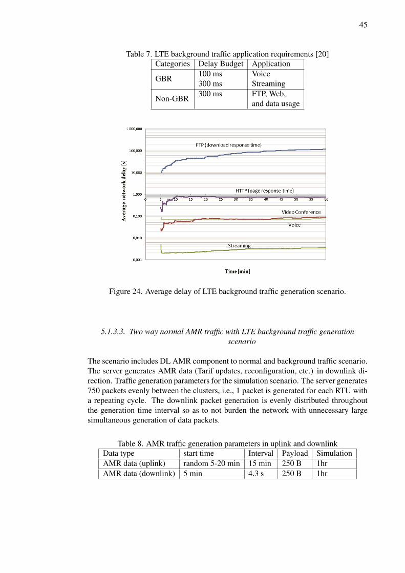
45

Table 7. LTE background traffic application requirements [20]Categories Delay Budget Application

GBR 100 ms Voice300 ms Streaming

Non-GBR 300 ms FTP, Web,and data usage

Figure 24. Average delay of LTE background traffic generation scenario.

5.1.3.3. Two way normal AMR traffic with LTE background traffic generationscenario

The scenario includes DL AMR component to normal and background traffic scenario.The server generates AMR data (Tarif updates, reconfiguration, etc.) in downlink di-rection. Traffic generation parameters for the simulation scenario. The server generates750 packets evenly between the clusters, i.e., 1 packet is generated for each RTU witha repeating cycle. The downlink packet generation is evenly distributed throughoutthe generation time interval so as to not burden the network with unnecessary largesimultaneous generation of data packets.

Table 8. AMR traffic generation parameters in uplink and downlinkData type start time Interval Payload SimulationAMR data (uplink) random 5-20 min 15 min 250 B 1hrAMR data (downlink) 5 min 4.3 s 250 B 1hr

46

Figure 25. Average load of two way normal AMR traffic with LTE background trafficgeneration scenario.

Figure 26. Average delay of two way normal AMR traffic with LTE background trafficgeneration scenario.

The Table 8 shows the traffic generation parameters. The average generated uplinkand downlink traffic along with the AMR component is shown in the Figure 25. TheFigure 26 shows the average network delay as a function of time. The DL AMR trafficis shown in this plot is less compared to previous BG and normal scenario. The delayfor DL AMR is found to be bit more than 2 ms. The obtained results are comparedwith the NIST [9] smart metering requirements in Table 11.

47

5.2. Sensor Network

We have seen that AMR data produced in the LTE network does not effect the load anddelay performance of the network. In this section we use sensor nodes instead of LTEdevices. The chosen sensor network model for performing the simulations is basedon [52].

5.2.1. Topology description

The sensor network simulations are done on suburban environment, as depicted inFigure 20. The topology stated in the LTE network model is used for sensor networksimulations. The parameters used for simulating sensor nodes are described in Table 9.

Table 9. Simulation parameters of WSN in smart metersPhysical layer parameters

Data rate 250 KbpsBandwidth 2000 KhzFrequency 2401 MhzNoise figure 1 dB

MAC layer parametersBeacon order 7Superframe order 7Number of retransmissions 4CSMA backoff number 5CSMA backoff exponent 3Beacon enabled yes

Application layer parametersTraffic generated Best effort trafficPacket inter arrival time 600 sPacket size 2000 bits

5.2.2. Propagation model

The sensor node in the simulations use free space pathloss model for evaluatingpathloss during propagation. The free space pathloss [48] is given by:

PLf = A+ 10�log10(dpl/dpl0) + s; d d0 (5.2)

where A is the free space path loss constant, s is shadow fading component, dpl is thedistance separation between the transmitter and receiver, dpl0 is the reference distance

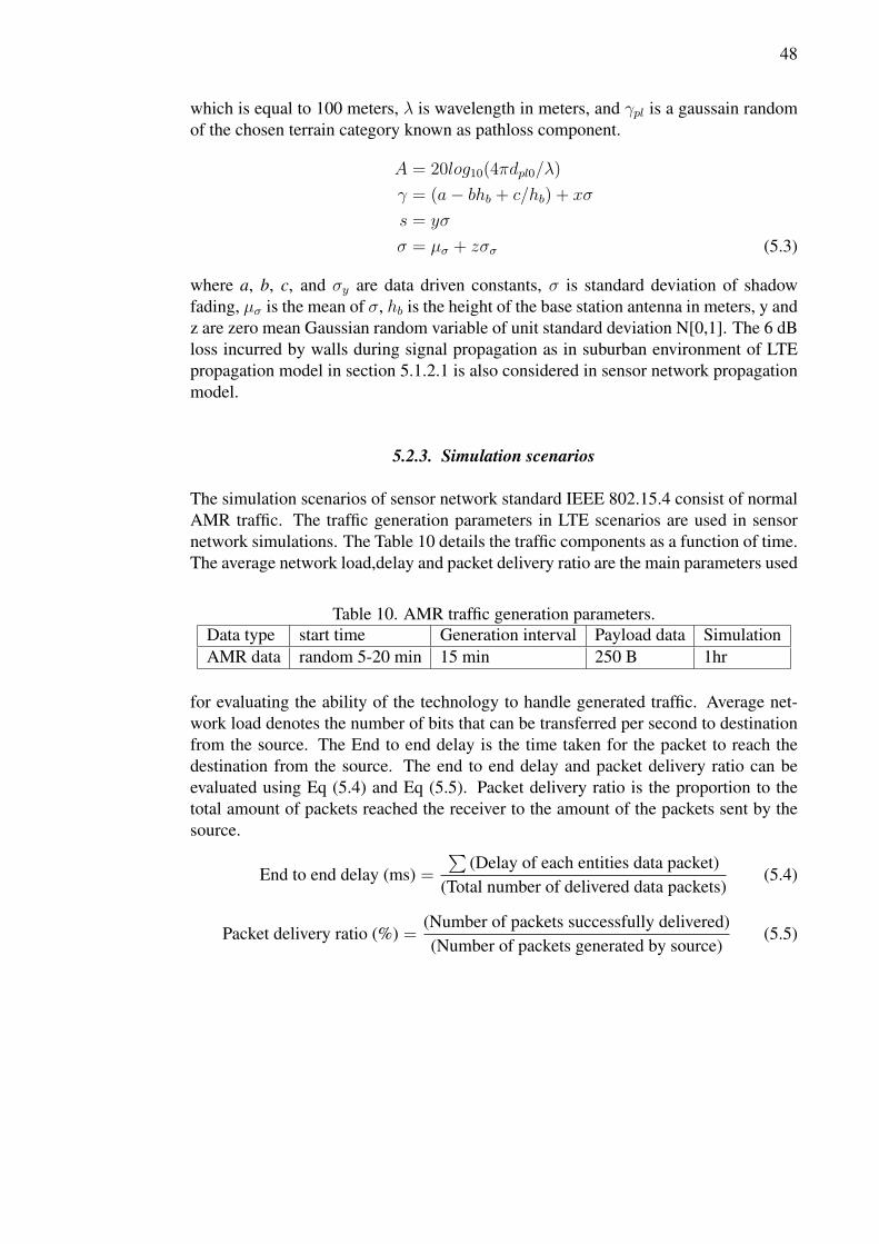
48

which is equal to 100 meters, � is wavelength in meters, and �pl is a gaussain randomof the chosen terrain category known as pathloss component.

A = 20log10(4⇡dpl0/�)

� = (a� bhb + c/hb) + x�

s = y�

� = µ� + z�� (5.3)

where a, b, c, and �y are data driven constants, � is standard deviation of shadowfading, µ� is the mean of �, hb is the height of the base station antenna in meters, y andz are zero mean Gaussian random variable of unit standard deviation N[0,1]. The 6 dBloss incurred by walls during signal propagation as in suburban environment of LTEpropagation model in section 5.1.2.1 is also considered in sensor network propagationmodel.

5.2.3. Simulation scenarios

The simulation scenarios of sensor network standard IEEE 802.15.4 consist of normalAMR traffic. The traffic generation parameters in LTE scenarios are used in sensornetwork simulations. The Table 10 details the traffic components as a function of time.The average network load,delay and packet delivery ratio are the main parameters used

Table 10. AMR traffic generation parameters.Data type start time Generation interval Payload data SimulationAMR data random 5-20 min 15 min 250 B 1hr

for evaluating the ability of the technology to handle generated traffic. Average net-work load denotes the number of bits that can be transferred per second to destinationfrom the source. The End to end delay is the time taken for the packet to reach thedestination from the source. The end to end delay and packet delivery ratio can beevaluated using Eq (5.4) and Eq (5.5). Packet delivery ratio is the proportion to thetotal amount of packets reached the receiver to the amount of the packets sent by thesource.

End to end delay (ms) =P

(Delay of each entities data packet)(Total number of delivered data packets)

(5.4)

Packet delivery ratio (%) =(Number of packets successfully delivered)(Number of packets generated by source)

(5.5)

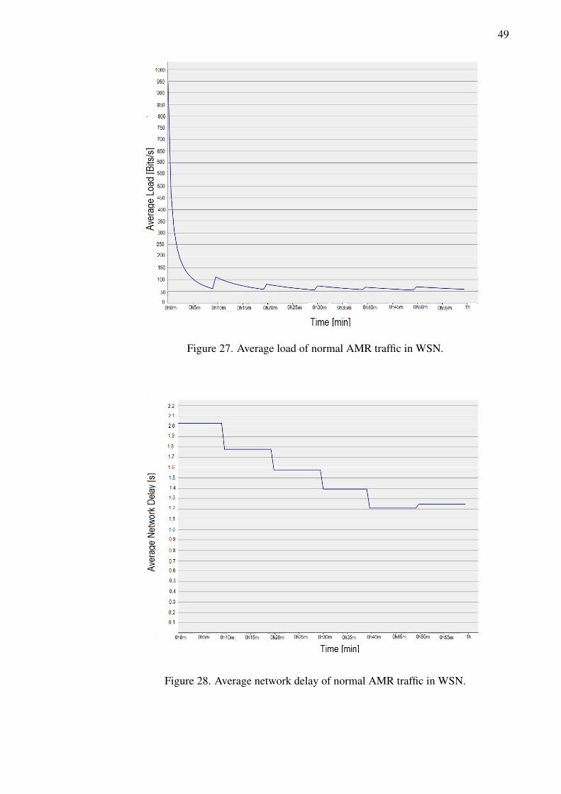
49

Figure 27. Average load of normal AMR traffic in WSN.

Figure 28. Average network delay of normal AMR traffic in WSN.

50

The Figure 27 visualizes the average network load of AMR traffic using WSN. Thecommunication of data with the coordinator from 25 nodes show a exponential de-crease from 900 to 60 Kbps. The average load is found to be 80 Kbps with payloadof 250 Bytes. The Figure 28 shows the network end to end delay with normal traf-fic components as function of time. The average end to end delay is found to be 1.6seconds. To summarise the Figures 27 and 28 the traffic load and the network end toend delay values are below the tolerable level specified by NIST [9] requirements forsmart metering. The Table 11 summarise the LTE and WSN simulation output resultsdetailed in the Section 5.3.

5.3. Discussion

The main aspect of the simulation study detailed in Sections 5.2.3, and 5.1.3 is tounderstand the feasibility of LTE and WSN communication techonologies for smartmeters. The feasibility study compares the results of LTE and WSN with the require-ments by NIST [9] as shown in Table 11. The data aggregation point (DAP) to smartmeter is considered as downlink and smart meter to DAP as uplink communication.

Table 11. Feasibility study of LTE and WSN in smart metersNIST [9] requirements for smart metering

Parameter ValueAverage delay (seconds) <10Average payload (Bytes) 200 to 1600Use cases (specific to NIST [9]) MR-14, MR-16, MR-26, MR-27, MR-35Reliability 99%

Smart meters using LTE technologyParameter Uplink DownlinkAverage delay (seconds) 3E-02 3E-03Average payload (Bytes) 250 250Data rate (bits/sec) 0.3k 0.08k

Smart meters using WSN technologyParameter DownlinkAverage delay (seconds) 1.6Average payload (Bytes) 250Data rate (bits/sec) 50

The simulation results validate the feasibility of LTE and WSN communications insmart meters with respect to NIST [9] requirements. The average delay accordingto the NIST [9] smart metering requirements is less than 10 seconds for a payloadranging from 200 to 1600 Bytes of packet data. The simulations are performed forpayload packet data of 250 Bytes for both LTE and WSN in suburban environment.The delay due to smart metering traffic is found to 3⇥ 10

�03s for LTE communication

technology and 1,6s for WSN communication technology.

51

6. FRAGMENTATION ANALYSIS IN THE MAC LAYER OFIEEE 802.15.4K STANDARD

6.1. Introduction

In this chapter the suitable size for handling smart meter traffic in WSN is evaluatedusing fragmentation scheme. Each fragment has a error control code to mitigate theerrors that occur in the wireless communication channel. The WSN uses CRC codein the MAC layer. CRC codes are error detecting codes which are used in digitalcommunication networks for link reliability and in storage devices to protect the data.CRC code was invented by W. Wesley Peterson [53] in the year 1961.

In LECIM draft (i.e., IEEE 802.15.4k [10] which can be used for smart meteringapplications in sensor node devices) the frames in the MAC layer are fragmented. Thewhole MAC frame of IEEE 802.15.4 [12] is divided in to equal sized fragments. Now,each fragment requires separate CRC code attached for the reliability of the fragmentdata received. In this chapter the appropriate fragment and CRC checksum size foreach fragment of divided MAC frame in the IEEE 802.15.4k standard is evaluatedusing undetected error probability. The generator polynomials used for different CRCchecksums (i.e, 8, 16, 24, and 32 bits) are shown in 6.1 [12], 6.2 [12], 6.3 [54], and6.4 [27].

8 bit polynomial:x

8+ x

7+ x

4+ x

3+ x+ 1 (6.1)

16 bit polynomial:x

16+ x

12+ x

5+ 1 (6.2)

24 bit polynomial:x

24+ x

23+ x

6+ x

5+ x+ 1 (6.3)

32 bit polynomial:

x

32+x

26+x

23+x

22+x

16+x

12+x

11+x

10+x

8+x

7+x

5+x

4+x

2+x

1+1 (6.4)

The 8 bit CRC generator polynomial was proposed by Comité consultatif interna-tional téléphonique et télégraphique (CCITT) now renamed as international telecom-munication union - telecommunication standardization sector (ITU-T) [55]. The 8 bitgenerator polynomial is also used in asynchronous transfer mode (ATM), a switchingtechnique used in computer networks and in integrated services digital network (ISDN)a communication standard used for transmission of voice, data and other network ser-vices. The IEEE 802.15.4 standard [12] specifies the generator polynomials for 16 and32 bit. The 24 bit polynomial was proposed by Nokia to 3GPP [54].

6.2. Error performance analysis

The performance evaluation of linear block code (e.g., CRC code) depends on theprobability of undetected error [56] at the decoder. Errors at the decoder can be cat-egorized to detected or undetected errors. The detected errors can be corrected using

52

error recovery techniques (e.g., ARQ, FEC). For undetected errors, the error probabil-ity is evaluated which can provide the performance criteria of the used error detectioncode. The theoretical undetected error probability for CRC code of particular check-sum length [56] is given in 6.5.

Pue(C, ✏) =

nX

i=1

Ai✏i(1� ✏)

n�i, (6.5)

where Ai is the number of codewords of weight i in (n,k,d) linear block code C, and ✏

is the bit error rate of the channel (✏ 2 [0, 0,5]).Alternatively, the probability of undetected error can be evaluated by 6.6.

Pue(C, ✏) = 2

�m

nX

i=0

Bi(1� 2✏)

i � (1� ✏)

n, (6.6)

where Bi is the number of codewords of weight i in (n, k, d) linear block dual code CT ,m = n� k. The weight distributions Ai, Bi in Eq (6.5) and Eq (6.6) are

A(z) = A0 + A1z + A2z + · · ·+ Anz· (6.7)

B(z) = B0 +B1z +B2z + · · ·+Bnz· (6.8)

The weight distributions of the Ai and Bi are needed for evaluating undetected errorprobabilities. Different methods for the evaluation of weight distributions of Ai and Bi

are proposed in [57–59]. The calculation of weight distributions using the proposedmethods is complex and cumbersome. The easiest way to evaluate the weight dis-tributions is by assuming the weight distributions to a previously known distribution.To understand the complexity of determining weight distributions, let us take a linearblock code of (1040,1024) for example where n = 1040 bits and k = 1024 bits. Thecalculation of weight distribution of Ai for the block code (1040,1024) is obtained byevaluating all the codewords of weights equal to 21024 (i.e., 1.8* 10308), whereas thecalculation of weight distribution of Bi is evaluated using dual code. Dual code is thescalar product of the original code. Hence, the weight distribution of Bi result to 2m

codewords (i.e., 216 = 65536 codewords ). But, to derive the dual code weight distri-bution Bi can be much more tedious than the weight distribution Ai. To evaluate theweight distribution of Ai in this thesis, binomial distribution can be assumed as de-tailed in [60]. Then the equation to evaluate probability of undetected error probabilityis given by

Pue(✏) =

dmaxX

i=dmin

✓n

i

◆/2

m ⇤ (✏i(1� ✏)

n�i)· (6.9)

The theoretical upper bound of the undetected error for different polynomials isgiven by 2�m [61] where m is the redundancy of the code or the length of the paritycode. Hence, the theoretical upper bound values for 8, 16, 24, 32 bits are 3.9*10�03,1.52*10�05, 5.9*10�08, and 2.32*10�10 respectively.

53

6.3. Fragmentation scheme in IEEE 802.15.4k standard

In low energy, critical infrastructure monitoring (LECIM) networks, requires dividingthe whole data frame to several frames for higher reliability. The fragmentation is donein the MAC layer before sending it to the physical layer. The objective for fragmentingMAC frame to several smaller fragments is to avoid interference caused by low PHYoperating modes [10] and also to reduce retransmission costs for longer frames. Thefragmentation scheme of MAC service data unit (MSDU) in to several fragments isshown in the Figure 29. The MSDU is fragmented into several fragments form thephysical layer protocol data unit (PPDU). Each PPDU now consist of new header andvalidity check sequence.

Figure 29. Fragmentation in IEEE 802.15.4k [10].

The validity check sequence is the CRC checksum obtained through polynomialdivision as detailed in Section 4.1.1. The different polynomials chosen for evaluatingthe checksum are specified in Section 6.1. Different fragment lengths where the MACframe can be fragmented are considered. The sizes considered are shown in table 12.The size of MSDU according the IEEE 802.15.4 standard [12] is 127 bytes which is1016 binary bits.

The MSDU frame format according the IEEE 802.15.4 standard [12] is shown in theFigure 30.

Figure 30. MAC Frame format [12] of IEEE 802.15.4 Standard.MHR (24 bits) MSDU (1016 bits) FCS (32 bits)

The MAC layer frame shown in Figure 30 is divided in to many fragments. Thefragmented frame consist of fields shown in Figure 31. The fragmented frame is com-posed of the fragment header which can be 1 to 3 bytes variable depending the PHYprofile [12], the fragment payload data and the validity check sequence (i.e., framecheck sequence (FCS)).

If the frame cannot be divided exactly in to chosen fragment sizes (i.e., 2,4,8,· · · ,1024) then bit stuffing is performed. In bit stuffing, MAC frame is appended with zeros

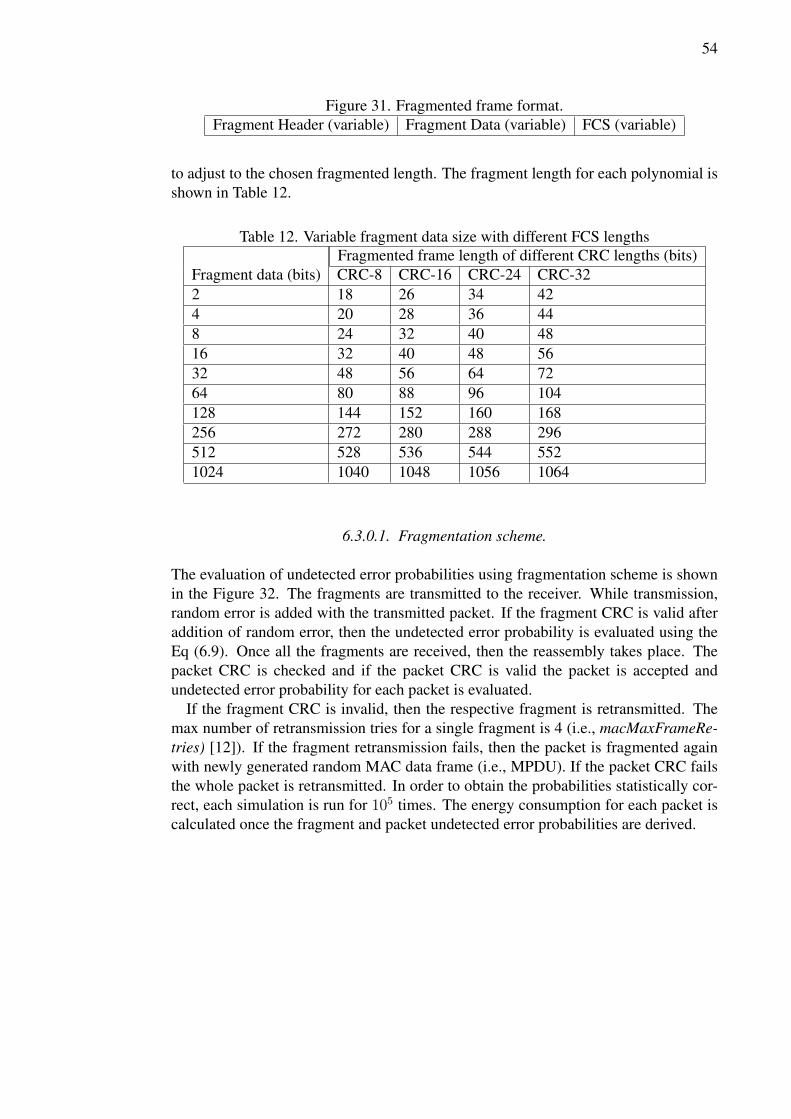
54

Figure 31. Fragmented frame format.Fragment Header (variable) Fragment Data (variable) FCS (variable)

to adjust to the chosen fragmented length. The fragment length for each polynomial isshown in Table 12.

Table 12. Variable fragment data size with different FCS lengthsFragmented frame length of different CRC lengths (bits)

Fragment data (bits) CRC-8 CRC-16 CRC-24 CRC-322 18 26 34 424 20 28 36 448 24 32 40 4816 32 40 48 5632 48 56 64 7264 80 88 96 104128 144 152 160 168256 272 280 288 296512 528 536 544 5521024 1040 1048 1056 1064

6.3.0.1. Fragmentation scheme.

The evaluation of undetected error probabilities using fragmentation scheme is shownin the Figure 32. The fragments are transmitted to the receiver. While transmission,random error is added with the transmitted packet. If the fragment CRC is valid afteraddition of random error, then the undetected error probability is evaluated using theEq (6.9). Once all the fragments are received, then the reassembly takes place. Thepacket CRC is checked and if the packet CRC is valid the packet is accepted andundetected error probability for each packet is evaluated.

If the fragment CRC is invalid, then the respective fragment is retransmitted. Themax number of retransmission tries for a single fragment is 4 (i.e., macMaxFrameRe-tries) [12]). If the fragment retransmission fails, then the packet is fragmented againwith newly generated random MAC data frame (i.e., MPDU). If the packet CRC failsthe whole packet is retransmitted. In order to obtain the probabilities statistically cor-rect, each simulation is run for 105 times. The energy consumption for each packet iscalculated once the fragment and packet undetected error probabilities are derived.

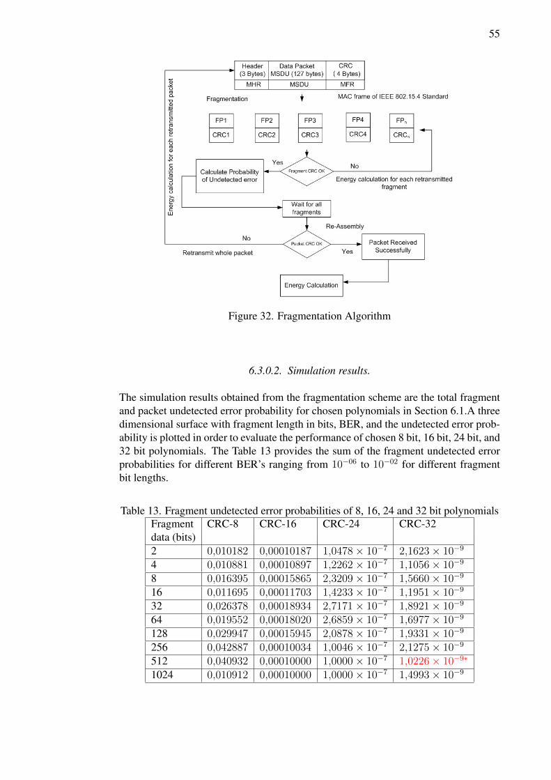
55

Figure 32. Fragmentation Algorithm

6.3.0.2. Simulation results.

The simulation results obtained from the fragmentation scheme are the total fragmentand packet undetected error probability for chosen polynomials in Section 6.1.A threedimensional surface with fragment length in bits, BER, and the undetected error prob-ability is plotted in order to evaluate the performance of chosen 8 bit, 16 bit, 24 bit, and32 bit polynomials. The Table 13 provides the sum of the fragment undetected errorprobabilities for different BER’s ranging from 10

�06 to 10

�02 for different fragmentbit lengths.

Table 13. Fragment undetected error probabilities of 8, 16, 24 and 32 bit polynomialsFragment CRC-8 CRC-16 CRC-24 CRC-32data (bits)2 0,010182 0,00010187 1,0478⇥ 10

�72,1623⇥ 10

�9

4 0,010881 0,00010897 1,2262⇥ 10

�71,1056⇥ 10

�9

8 0,016395 0,00015865 2,3209⇥ 10

�71,5660⇥ 10

�9

16 0,011695 0,00011703 1,4233⇥ 10

�71,1951⇥ 10

�9

32 0,026378 0,00018934 2,7171⇥ 10

�71,8921⇥ 10

�9

64 0,019552 0,00018020 2,6859⇥ 10

�71,6977⇥ 10

�9

128 0,029947 0,00015945 2,0878⇥ 10

�71,9331⇥ 10

�9

256 0,042887 0,00010034 1,0046⇥ 10

�72,1275⇥ 10

�9

512 0,040932 0,00010000 1,0000⇥ 10

�71,0226⇥ 10

�9⇤

1024 0,010912 0,00010000 1,0000⇥ 10

�71,4993⇥ 10

�9

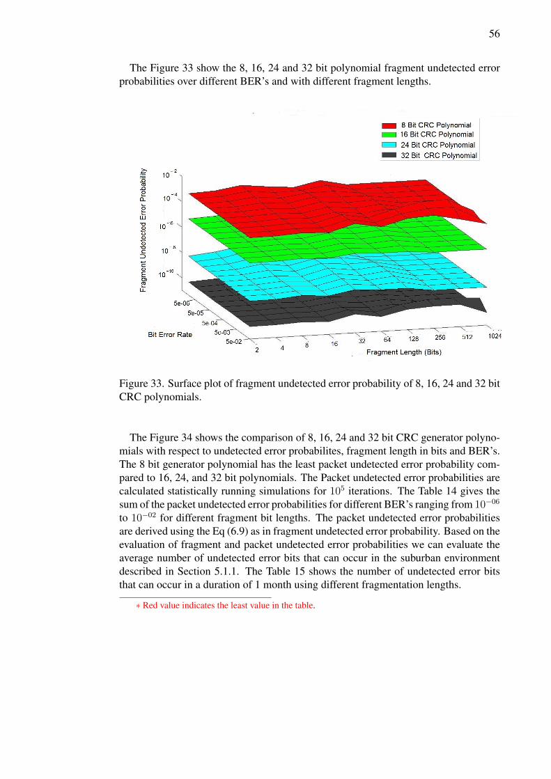
56

The Figure 33 show the 8, 16, 24 and 32 bit polynomial fragment undetected errorprobabilities over different BER’s and with different fragment lengths.

Figure 33. Surface plot of fragment undetected error probability of 8, 16, 24 and 32 bitCRC polynomials.

The Figure 34 shows the comparison of 8, 16, 24 and 32 bit CRC generator polyno-mials with respect to undetected error probabilites, fragment length in bits and BER’s.The 8 bit generator polynomial has the least packet undetected error probability com-pared to 16, 24, and 32 bit polynomials. The Packet undetected error probabilities arecalculated statistically running simulations for 105 iterations. The Table 14 gives thesum of the packet undetected error probabilities for different BER’s ranging from 10

�06

to 10

�02 for different fragment bit lengths. The packet undetected error probabilitiesare derived using the Eq (6.9) as in fragment undetected error probability. Based on theevaluation of fragment and packet undetected error probabilities we can evaluate theaverage number of undetected error bits that can occur in the suburban environmentdescribed in Section 5.1.1. The Table 15 shows the number of undetected error bitsthat can occur in a duration of 1 month using different fragmentation lengths.

⇤ Red value indicates the least value in the table.

57

Figure 34. Surface plot of packet undetected error probability of 8, 16, 24 and 32 bitCRC polynomials.

Table 14. Packet undetected error probabilities of 8, 16, 24 and 32 bit polynomialsFragment CRC-8 CRC-16 CRC-24 CRC-32data (bits)2 3,5605⇥ 10

�123,5572⇥ 10

�123,5538⇥ 10

�123,5549⇥ 10

�12

4 1,3610⇥ 10

�111,3531⇥ 10

�111,3446⇥ 10

�111,3472⇥ 10

�11

8 1,0901⇥ 10

�101,0313⇥ 10

�109,9640⇥ 10

�119,9872⇥ 10

�11

16 2,5749⇥ 10

�112,5445⇥ 10

�112,5138⇥ 10

�112,5231⇥ 10

�11

32 4,7174⇥ 10

�102,8306⇥ 10

�103,6718⇥ 10

�102,6093⇥ 10

�11

64 1,8830⇥ 10

�101,6980⇥ 10

�101,6513⇥ 10

�101,6223⇥ 10

�11

128 5,7806⇥ 10

�101,8333⇥ 10

�104,1426⇥ 10

�101,6319⇥ 10

�11

256 6,9572⇥ 10

�101,5377⇥ 10

�124,6504⇥ 10

�101,3816⇥ 10

�12

512 6,9830⇥ 10

�101,5200⇥ 10

�124,6665⇥ 10

�101,6800⇥ 10

�12

1024 1,2702⇥ 10

�121,8900⇥ 10

�121,2802⇥ 10

�121,2600⇥ 10

�12⇤

The Table 14 shows the sum probabilities of packet undetected errors. From theTable 14 the packet undetected error probabilities are found to be the least for 2 and1024 bits with values ranging to 10

�12 for all the CRC Polynomials. It can also beseen that 16, and 32 bit CRC polynomials showing a similar profile while 8, and 24bit exhibiting a similar packet undetected error profile. If we consider the 8 bit and24 bit CRC polynomials for the packet undetected error values, as the fragment sizeincreases the undetected error probability increases and decreases until 16 bit frag-ment length and remains constant till 512 bit fragment length and decreases for 1024

⇤ Red value indicates the least value in the table.

58

bits. The reason behind this fluctuating error probabilities might be due to the lengthof the payload and CRC for each packet. If we consider the 16, and 32 bit polyno-mial, the undetected error probabilities also increase until 128 bit fragment length anddecrease as the fragment length increases. It can inferred from the result that 16 bitand 32 bit polynomials are better compared to 8 and 24 bit Polynomial with respectto packet undetected error probabilities. Based on the fragment and packet undetectederror probabilities we can derive the average number of possible undetected error bitsin particular duration of time (i.e., 30 days) as shown in Table 15. As the packet er-ror probabilities and fragment error probabilities are least for 2 and 1024 bit fragmentlengths, the occurence of undetected error bits are also the least. The undetected errorbits (i.e., 1,2609) is found to be the least for 512 bit fragment length with CRC poly-nomial of 32 bit length. The probability of undetected error bits are evaluated usingTable 5. The AMR traffic is generated every 15 min with packet size of 250 Bytes.Hence the total number of packets for 30 days is evaluated. The packet undetectederror probabilities are multiplied with the number of packets to determine the numberof bits which can be undetected at the receiver in a duration of 30 days.

Table 15. Average undetected error bits of 8, 16, 24 and 32 bit polynomialsFragment CRC-8 CRC-16 CRC-24 CRC-32data (bits)2 1,2660 1,2618 1,2616 1,2680

4 1,5162 1,5542 1,5621 1,5658

8 1,8895 1,8956 1,5061 1,5156

16 1,5172 1,5041 1,545 1,5074

32 1,8155 1,8758 1,8111 1,8520

64 1,7742 1,7818 1,8836 1,8477

128 1,8367 1,7388 1,8802 1,8595

256 1,8600 1,2768 1,8008 1,2895

512 1,8282 1,2681 1,8322 1,2609

⇤

1024 1,2703 1,2611 1,2630 1,2772

6.4. Energy evaluation analysis

WSNs consist of a set of small devices with limited energy resources, reduced process-ing capabilities and a radio frequency communication unit with limited transmissionpower. Power consumption models [62] in sensor nodes take both transceiver andstartup power consumption along with an accurate model of the amplifier as shown inFigure 35. The power consumption energy per bit eb [63] can be given as

eb = etx + erx + Edec/ı, (6.10)where etx and erx are the transmitter and receiver power energy consumption per bit,respectively, Edec is the energy required for decoding a packet, and ı is the payloadlength in bits. The etx from Eq (6.10) can be given by

⇤ Red value indicates the least value in the table.

59

etx = ete + etad↵, (6.11)

where ete is the energy consumption of the transmitter electronics per bit, eta is theenergy consumption of the transmit amplifier per bit over a distance of 1 meter, d is thetransmission distance, and ↵ is the pathloss component. The expression for evaluatingthe transmit amplifier per bit over a distance of 1 meter [64] can be given by

eta =(S/N)r(NFRx)(N0)(BW )(4⇡/�)

↵

(Gant)(⌘amp)(Rbit)(6.12)

where (S/N)r, is the desired signal to noise ratio at the receiver demodulator, NFRx isthe receiver noise figure, N0 is the thermal noise floor for 1 Hz bandwidth, BW is thechannel noise bandwidth, � is the wavelength in meters, Gant is the antenna gain,⌘amp

is the transmitter efficiency, Rbit is the raw channel rate in bits per second.The Eq (6.10)takes into account the energy needed to transmit a frame from a transmitter to a receiverover single hop. The Figure 35 shows the transmitter and receiver energy consumptioncomponents when k bits are transmitted to the receiver.

Figure 35. Typical radio energy consumption model where k bits are transmitted,ete and eta are the transmitter electronics and amplifier energy consumption per bit,respectively. The transmission distance is d and the k bits are received by the receiver,consuming erx energy per bit [62].

The parameters used for determining the energy consumption values of the transmit-ter and receiver are shown in Table 16.

Table 16. Radio parameters of sensor nodeParameter ValueTransmitter circuitry (ete) 1.066 µJ/bit

Receiver circuitry (erx) 0.533 µJ/bit

Receiver noise figure (NFrx) 10 dBThermal noise floor (N0) 4.17*10�21JBandwidth (BW) 40000 HzFrequency (f) 900 MHzWavelength (�) 0.333 mPath loss exponent (↵) 2.5Antenna gain (Gant) 0 dBTransmitter efficiency (⌘amp) 0.2Signal to Noise Ratio (S/N)r 10 dBRaw bit rate (Rbit) 37500 bps

60

The PHY profile of the 802.15.4 [12] standard can employ different modulationschemes as stated in chapter 2. Different modulation schemes results in different sig-nal to noise ratios (SNR). In order to understand the energy consumption per bit, weassume that sensor node is IEEE 802.15.4 [10] with the respective parameters shown inTable 16. The energy consumption per bit in joules per each fragment when transmittedusing different fragment lengths, BER, and polynomials is evaluated. The respectivesurface plot is shown in Figure 36. The surfaces shows the consumed energy per eachpolynomial while using the parameters from the Table 16.

Figure 36. Surface plot of energy consumption of 8, 16, 24 and 32 bit CRC polynomi-als.

The Figure 36 represent the energy consumption per bit while transmitting fragmentlengths shown in Table 12. The graph shows the energy consumption per payloadbit for each polynomial when transmitting a 1024 bit payload using fragment sizesbetween 2 and 1024 and taking into account overhead of fragmentation and CRC. Thealgorithm considers the retransmission of each fragment with retransmission whichequals to 4, if the CRC fails. Even after retransmission if the packet is not received,the packet is discarded and new packet is sent. From the fragmentation algorithmshown in Figure 32 transmitted and retransmitted packets are evaluated. Using thetransmitted and retransmitted packets, the delivery ratios are evaluated. The deliveryratios and energy consumption per bit shown in Eq (6.10) is used to evaluate the energyconsumption of each packet for a particular fragment length, CRC polynomial andBER. The energy consumptions of the polynomials are determined statistically for 105simulation iterations. The energy consumption for different BER’s (i.e., 10�2 to 10

�6)using CRC-8, 16, 24, and 32 is shown in Table 17, 18, 19, 20, and 21.

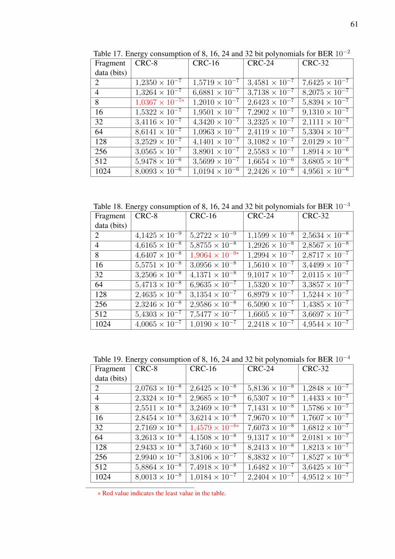
61

Table 17. Energy consumption of 8, 16, 24 and 32 bit polynomials for BER 10

�2

Fragment CRC-8 CRC-16 CRC-24 CRC-32data (bits)2 1,2350⇥ 10

�71,5719⇥ 10

�73,4581⇥ 10

�77,6425⇥ 10

�7

4 1,3264⇥ 10

�76,6881⇥ 10

�73,7138⇥ 10

�78,2075⇥ 10

�7

8 1,0367⇥ 10

�7⇤1,2010⇥ 10

�72,6423⇥ 10

�75,8394⇥ 10

�7

16 1,5322⇥ 10

�71,9501⇥ 10

�77,2902⇥ 10

�79,1310⇥ 10

�7

32 3,4116⇥ 10

�74,3420⇥ 10

�73,2325⇥ 10

�72,1111⇥ 10

�7

64 8,6141⇥ 10

�71,0963⇥ 10

�72,4119⇥ 10

�75,3304⇥ 10

�7

128 3,2529⇥ 10

�74,1401⇥ 10

�73,1082⇥ 10

�72,0129⇥ 10

�7

256 3,0565⇥ 10

�73,8901⇥ 10

�72,5583⇥ 10

�71,8914⇥ 10

�6

512 5,9478⇥ 10

�63,5699⇥ 10

�71,6654⇥ 10

�63,6805⇥ 10

�6

1024 8,0093⇥ 10

�61,0194⇥ 10

�62,2426⇥ 10

�64,9561⇥ 10

�6

Table 18. Energy consumption of 8, 16, 24 and 32 bit polynomials for BER 10

�3

Fragment CRC-8 CRC-16 CRC-24 CRC-32data (bits)2 4,1425⇥ 10

�95,2722⇥ 10

�91,1599⇥ 10

�82,5634⇥ 10

�8

4 4,6165⇥ 10

�85,8755⇥ 10

�81,2926⇥ 10

�82,8567⇥ 10

�8

8 4,6407⇥ 10

�81,9064⇥ 10

�9⇤1,2994⇥ 10

�72,8717⇥ 10

�7

16 5,5751⇥ 10

�83,0956⇥ 10

�81,5610⇥ 10

�73,4499⇥ 10

�7

32 3,2506⇥ 10

�84,1371⇥ 10

�89,1017⇥ 10

�72,0115⇥ 10

�7

64 5,4713⇥ 10

�86,9635⇥ 10

�71,5320⇥ 10

�73,3857⇥ 10

�7

128 2,4635⇥ 10

�83,1354⇥ 10

�76,8979⇥ 10

�71,5244⇥ 10

�7

256 2,3246⇥ 10

�82,9586⇥ 10

�86,5090⇥ 10

�71,4385⇥ 10

�7

512 5,4303⇥ 10

�77,5477⇥ 10

�71,6605⇥ 10

�73,6697⇥ 10

�7

1024 4,0065⇥ 10

�71,0190⇥ 10

�72,2418⇥ 10

�74,9544⇥ 10

�7

Table 19. Energy consumption of 8, 16, 24 and 32 bit polynomials for BER 10

�4

Fragment CRC-8 CRC-16 CRC-24 CRC-32data (bits)2 2,0763⇥ 10

�82,6425⇥ 10

�85,8136⇥ 10

�81,2848⇥ 10

�7

4 2,3324⇥ 10

�82,9685⇥ 10

�86,5307⇥ 10

�81,4433⇥ 10

�7

8 2,5511⇥ 10

�83,2469⇥ 10

�87,1431⇥ 10

�81,5786⇥ 10

�7

16 2,8454⇥ 10

�83,6214⇥ 10

�87,9670⇥ 10

�81,7607⇥ 10

�7

32 2,7169⇥ 10

�81,4579⇥ 10

�8⇤7,6073⇥ 10

�81,6812⇥ 10

�7

64 3,2613⇥ 10

�84,1508⇥ 10

�89,1317⇥ 10

�82,0181⇥ 10

�7

128 2,9433⇥ 10

�83,7460⇥ 10

�88,2413⇥ 10

�81,8213⇥ 10

�7

256 2,9940⇥ 10

�73,8106⇥ 10

�78,3832⇥ 10

�71,8527⇥ 10

�6

512 5,8864⇥ 10

�87,4918⇥ 10

�81,6482⇥ 10

�73,6425⇥ 10

�7

1024 8,0013⇥ 10

�81,0184⇥ 10

�72,2404⇥ 10

�74,9512⇥ 10

�7

⇤ Red value indicates the least value in the table.

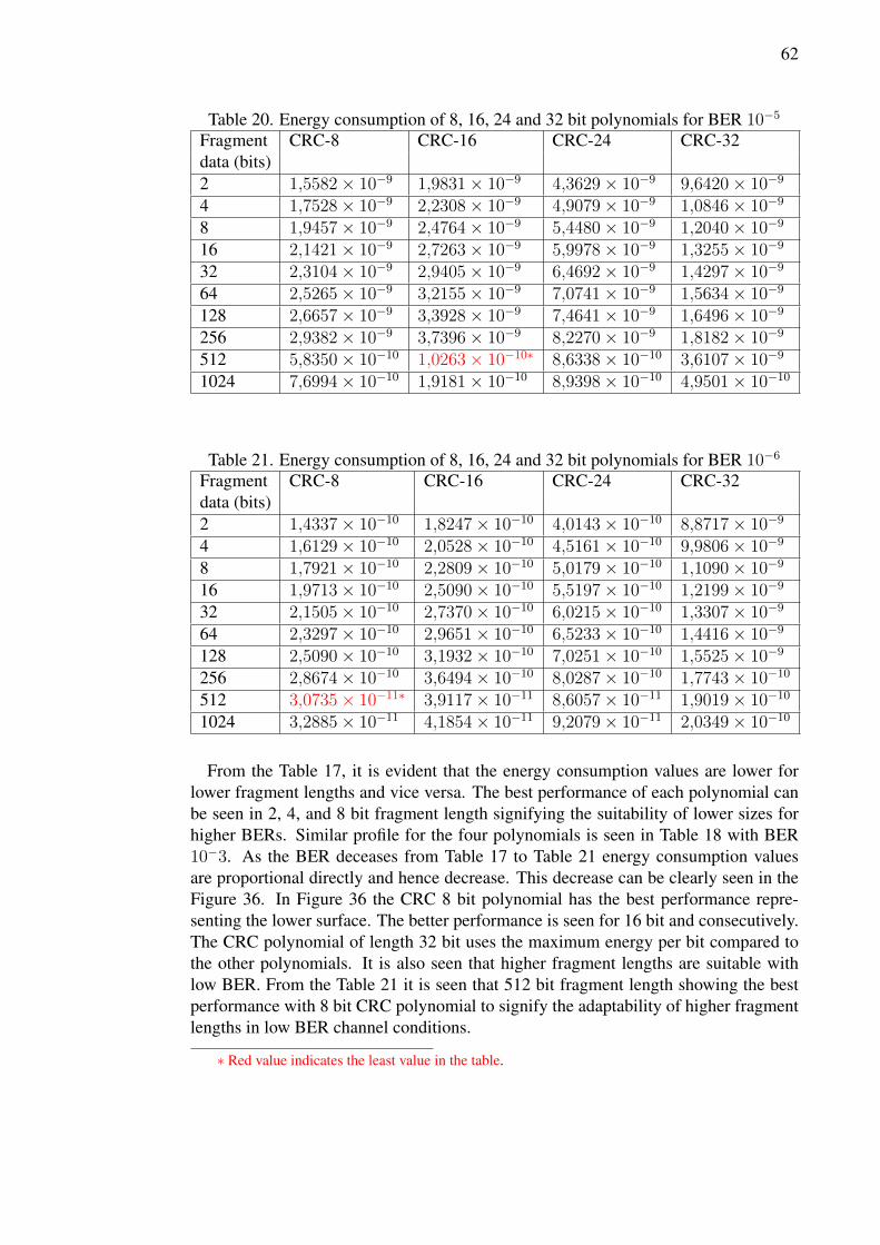
62

Table 20. Energy consumption of 8, 16, 24 and 32 bit polynomials for BER 10

�5

Fragment CRC-8 CRC-16 CRC-24 CRC-32data (bits)2 1,5582⇥ 10

�91,9831⇥ 10

�94,3629⇥ 10

�99,6420⇥ 10

�9

4 1,7528⇥ 10

�92,2308⇥ 10

�94,9079⇥ 10

�91,0846⇥ 10

�9

8 1,9457⇥ 10

�92,4764⇥ 10

�95,4480⇥ 10

�91,2040⇥ 10

�9

16 2,1421⇥ 10

�92,7263⇥ 10

�95,9978⇥ 10

�91,3255⇥ 10

�9

32 2,3104⇥ 10

�92,9405⇥ 10

�96,4692⇥ 10

�91,4297⇥ 10

�9

64 2,5265⇥ 10

�93,2155⇥ 10

�97,0741⇥ 10

�91,5634⇥ 10

�9

128 2,6657⇥ 10

�93,3928⇥ 10

�97,4641⇥ 10

�91,6496⇥ 10

�9

256 2,9382⇥ 10

�93,7396⇥ 10

�98,2270⇥ 10

�91,8182⇥ 10

�9

512 5,8350⇥ 10

�101,0263⇥ 10

�10⇤8,6338⇥ 10

�103,6107⇥ 10

�9

1024 7,6994⇥ 10

�101,9181⇥ 10

�108,9398⇥ 10

�104,9501⇥ 10

�10

Table 21. Energy consumption of 8, 16, 24 and 32 bit polynomials for BER 10

�6

Fragment CRC-8 CRC-16 CRC-24 CRC-32data (bits)2 1,4337⇥ 10

�101,8247⇥ 10

�104,0143⇥ 10

�108,8717⇥ 10

�9

4 1,6129⇥ 10

�102,0528⇥ 10

�104,5161⇥ 10

�109,9806⇥ 10

�9

8 1,7921⇥ 10

�102,2809⇥ 10

�105,0179⇥ 10

�101,1090⇥ 10

�9

16 1,9713⇥ 10

�102,5090⇥ 10

�105,5197⇥ 10

�101,2199⇥ 10

�9

32 2,1505⇥ 10

�102,7370⇥ 10

�106,0215⇥ 10

�101,3307⇥ 10

�9

64 2,3297⇥ 10

�102,9651⇥ 10

�106,5233⇥ 10

�101,4416⇥ 10

�9

128 2,5090⇥ 10

�103,1932⇥ 10

�107,0251⇥ 10

�101,5525⇥ 10

�9

256 2,8674⇥ 10

�103,6494⇥ 10

�108,0287⇥ 10

�101,7743⇥ 10

�10

512 3,0735⇥ 10

�11⇤3,9117⇥ 10

�118,6057⇥ 10

�111,9019⇥ 10

�10

1024 3,2885⇥ 10

�114,1854⇥ 10

�119,2079⇥ 10

�112,0349⇥ 10

�10

From the Table 17, it is evident that the energy consumption values are lower forlower fragment lengths and vice versa. The best performance of each polynomial canbe seen in 2, 4, and 8 bit fragment length signifying the suitability of lower sizes forhigher BERs. Similar profile for the four polynomials is seen in Table 18 with BER10

�3. As the BER deceases from Table 17 to Table 21 energy consumption values

are proportional directly and hence decrease. This decrease can be clearly seen in theFigure 36. In Figure 36 the CRC 8 bit polynomial has the best performance repre-senting the lower surface. The better performance is seen for 16 bit and consecutively.The CRC polynomial of length 32 bit uses the maximum energy per bit compared tothe other polynomials. It is also seen that higher fragment lengths are suitable withlow BER. From the Table 21 it is seen that 512 bit fragment length showing the bestperformance with 8 bit CRC polynomial to signify the adaptability of higher fragmentlengths in low BER channel conditions.

⇤ Red value indicates the least value in the table.

63

6.5. Discussion

The simulation results signify the importance of considering the fragmentation in theMAC layer of IEEE 802.15.4k [10] standard. To consider the proposed fragmentationscheme, this thesis focusses mainly on the fragment and packet undetected error proba-bilities, probability of undetected error bits, and the energy consumption per bit. Fromthe fragment undetected error probability values, fragment length of 512 bits and CRCpolynomial of length 32 bits has the least fragment undetected error probability of1,0226 ⇥ 10

�9. The surface plot in Figure 33 shows the 8 bit polynomial surface onthe top signifying the maximum of undetected error probabilities. It can be concludedthat the higher the length of the CRC polynomial the higher is the reliability of the sys-tem with less undetected errors. The fragment undetected error probability simulationresults show the fragment length of 512 bits has the least undetected error probabilitywhile using CRC polynomial of length 32 bits. But while considering the whole packetundetected error probability, fragment length of 1024 bits with CRC polynomial of 32bits has the least probability of 1,2600 ⇥ 10

�12. The next aspect to be considered isthe occurrence of undetected error bits. The Table 15 shows the average number ofundetected error bits that can occur in a particular duration of time (e.g., 30 days). TheCRC polynomial of length 32 bit and the fragment payload of 512 bits length is foundto have the least undetected error bits (i.e., 1,2609). To summarise the results, the frag-mentation scheme reduce the probability of undetected errors and the occurrence ofundetected error bits. Hence, the MAC layer packet with fragmentation has the leastfragment and packet undetected error probability with least number of undetected errorbits in a particular duration of time.

If we consider energy consumption per bit for the proposed fragmentation scheme,the Table 21, 20, 19, 18, and 17 show the energy consumption per bit for different BER(i.e., 10�06 to 10

�02). For BER 10

�02 in Table 17, the 8 bit CRC polynomial has theleast energy consumption for 8 bits (i.e., 1,0367⇥ 10

�7), the least energy consumptionfor 16 bit CRC is 6,6881⇥10

�7 for 4 bit fragment length, and for 24 bit CRC, the leastenergy consumption is 7,2902 ⇥ 10

�7 for 16 bit fragment length and for 32 bit CRCpolynomial the least energy consumption is 8,2075 ⇥ 10

�7 for 4 bit fragment length.It can be inferred from these results collectively that the lower fragment lengths aremore suitable at higher bit error rate. If we consider BER 10

�03 in Table 18, theincrease in fragment length is directly proportional to an increase in energy consumedin transmission, reception, and decoding is higher. For BER 10

�03, the least energyconsumption per bit is found to be 1,9064⇥10

�9 for fragment length of 8 bit and CRCpolynomial of length 16 bit. For BER 10

�04, the same bit polynomial with fragmentlength of 32 bit is found have the least energy consumption with 1,4579 ⇥ 10

�8. ForBER 10

�05 the least energy consumption is 1,0263 ⇥ 10

�10 and for BER 10

�06 the512 bit with bit CRC polynomial have the least consumptions 3,0735 ⇥ 10

�11. Tosummarise the energy consumption per bit aspect, the 512 bit fragment length and CRCpolynomial with bit length of 8 bit has the least value (i.e., 3,0735⇥ 10

�11) . Hence itcan be concluded that, for different BER’s different fragment lengths are found to beeffective. But the energy consumption of 8 bit CRC polynomial with fragment lengthof 512 bit is relatively superior when compared to 16, 24, and 32 bit CRC polynomials.

64

7. CONCLUSION

The simulation parameters, scenarios and results of smart meters using LTE and WSNcommunication technologies were studied in this thesis. The first part of the thesisproblem was to identify whether smart meter traffic effects LTE and WSN traffic. Thefeasibility study was performed by evaluating end to end delay and average load ofsmart meters using LTE and WSN. The results of the end to end delays and averageload values posed by smart meter traffic were compared with the NIST [9] require-ments. The results validate that the values are well below the requirements specifiedby NIST. The usage of LTE in smart meter for smart metering can be a option buthigher spectrum utilization results in smaller cell sizes and other technologies (i.e.,WSN) can also become competitive alternatives.

In the second part of the thesis the required frame length for handling smart metertraffic was discussed. A new fragmentation scheme was proposed. Fragmentation is re-quired in WSN [12] devices reduce the channel coherence time as the present mediumaccess control (MAC) design suffers from collisions [65] during carrier sense multipleaccess (CSMA) algorithm in high contention environments. In order to avoid collisionsin the MAC layer during CSMA algorithm so as to confront the required higher datarates in physical layer of IEEE 802.15.4 [12] standard. The whole packet is divided into equal length fragments. Fragment lengths were assumed to be 2, 4, · · · , 1024 bits.The fragments were reconstructed again to form the complete packet at the receiver.The surface plot of fragment and packet undetected error probability was derived. Itis found that the CRC polynomial of length 32 bit with fragment length of 512 bitsshowing the least fragment undetected error probability. The packet undetected errorprobabilities were calculated after reconstructing the packet the receiver. The packetundetected error probabilities shows that the same CRC polynomial of length 32 bithas the least packet undetected error probability. But the fragment length of 1024 bitfor each packet has the least probability. This shows that fragment undetected prob-ability and packet undetected error probability result in different error performance.It was also seen that as the packet size increases packet undetected error probabilitydecreases while fragment undetected error probability is vice versa. It can be inferredfrom these results that if the WSN device opts to use fragmentation then the best suit-able length is fragment length of 512 bits with CRC polynomial of 32 bit length whilewithout fragmentation the packet size of 1024 bits have the best performance. If thefragment, and packet undetected error probabilities can be derived, the occurrence ofundetected error bits can also be evaluated. The results obtained in this thesis showthat the least number of undetected error bits occur for fragment length of 512 bitswith CRC polynomial 32 bit.

The energy consumption per bit for the fragmented sizes and the chosen polyno-mials (i.e., 8, 16, 24, and 32 bits) show that for different BERs different fragmentlengths were found to be effective. The least energy consumption profile was seen for8 bit CRC polynomial. The higher the length of the polynomial the higher was the en-ergy consumption with higher reliability. The energy consumption results signify thatfragment length of 512 bit with CRC polynomial of length 8 bit signifying the bestperformance compared to other fragment sizes and polynomials.

65

8. REFERENCES

[1] Massoud Amin S. & Wollenberg B. (2005) Toward a smart grid: power deliveryfor the 21st century. Power and Energy Magazine, IEEE 3, pp. 34 – 41.

[2] Momoh J. (2012) Smart Grid: Fundamentals of Design and Analysis. IEEE PressSeries on Power Engineering, Wiley. URL: http://books.google.nl/books?id=j8IFx-6vMloC.

[3] Rafiei M., Elmi S. & Zare A. (2012) Wireless communication protocols for smartmetering applications in power distribution networks. In: Electrical Power Dis-tribution Networks (EPDC), 2012 Proceedings of 17th Conference on, pp. 1 –5.

[4] Depuru S., Wang L., Devabhaktuni V. & Gudi N. (2011) Smart meters for powergrid; challenges, issues, advantages and status. In: Power Systems Conferenceand Exposition (PSCE), 2011 IEEE/PES, pp. 1 –7.

[5] IEEE draft standard for a convergent digital home network for heterogeneoustechnologies. IEEE P1905.1/D06, September 2012 , pp. 1 –125.

[6] Cuvelier P.K. & Sommereyns P. (2009) Proof of concept smart metering. In: Elec-tricity Distribution - Part 1, 2009. CIRED 2009. 20th International Conferenceand Exhibition on, pp. 1 –4.

[7] Koay B., Cheah S., Sng Y., Chong P., Shum P., Tong Y., Wang X., Zuo Y. & KuekH. (2003) Design and implementation of bluetooth energy meter. In: Information,Communications and Signal Processing, 2003 and Fourth Pacific Rim Confer-ence on Multimedia. Proceedings of the 2003 Joint Conference of the FourthInternational Conference on, pp. 1474 – 1477.

[8] Rusitschka S., Gerdes C. & Eger K. (2009) A low-cost alternative to smart meter-ing infrastructure based on peer-to-peer technologies. In: Energy Market, 2009.EEM 2009. 6th International Conference on the European, pp. 1 –6.

[9] JoeHughes (2010), Smart metering requirements ,pap02objective1 (ac-cessed on 01 Sep,2012)). URL: {http://collaborate.nist.gov/twiki-sggrid/bin/view/SmartGrid/PAP02Objective1/}.

[10] IEEE draft for local and metropolitan area networks-part 15.4: Low-rate wire-less personal area networks (wpans) amendment physical layer specifications forlow energy, critical infrastructure monitoring networks. IEEE D802.15.4k-2012(Amendment to IEEE Std 802.15.4-2011) .

[11] 3GPP,LTE overview (accessed on 08 oct 2012). URL: {http://www.3gpp.com/LTE}.

[12] IEEE standard for local and metropolitan area networks–part 15.4: Low-ratewireless personal area networks (LR-WPANs). IEEE Std 802.15.4-2011 (Revi-sion of IEEE Std 802.15.4-2006) , pp. 1 –314.

66

[13] Sauter M. (2010) From GSM to LTE: An Introduction to Mobile Networksand Mobile Broadband. Wiley Online Library: Books, Wiley. URL: http://books.google.nl/books?id=uso-6LN2YjsC.

[14] Holma H. & Toskala A. (2009) LTE for UMTS: OFDMA and SC-FDMAbased radio access. Wiley. URL: http://books.google.fi/books?id=AHr43Lh-roQC.

[15] 3GPP TS 33.401, "Digital cellular telecommunications system (phase2+); universal mobile telecommunications system (umts); 3GPP sys-tem architecture evolution (sae); security architecture (release 8)". URL:http://www.etsi.org/deliver/etsi_ts/133400_133499/133401/08.01.01_60/ts_133401v080101p.pdf.

[16] Poikselkä M. (2006) The IMS: IP multimedia concepts and services. J. Wiley &Sons. URL: http://books.google.fi/books?id=lBMfAQAAIAAJ.

[17] Mobile WiMAX part 1: A technical overview and performance eval-uation, WiMAX forum, white paper, august 2006, (accessed on 18sept 2012). URL: {http://www.ictregulationtoolkit.org/en/Publication.2952.html}.

[18] Digital video broadcasting (DVB): Framing structure, channel coding and mod-ulation for digital terrestrial television, etsi, ets en 300 744 v 1.1.2.

[19] Chang R.W. (1966) [duplicate] Synthesis of Band-Limited Orthogonal Signalsfor Multichannel Data Transmission. Bell Systems Technical Journal 45, pp.1775–1796.

[20] Khan F. (2009) LTE for 4G Mobile Broadband: Air Interface Technologies andPerformance. Cambridge University Press, New York, NY, USA, 1st ed.

[21] Dahlman E. (2008) 3G Evolution: HSPA and LTE for Mobile Broadband. Aca-demic Press, Academic. URL: http://books.google.fi/books?id=cmMgp4j23D0C.

[22] Myung H. & Goodman D. (2008) Single Carrier Fdma: A New Air Inter-face for Long Term Evolution. Wireless Communications and Mobile Comput-ing, John Wiley & Sons. URL: http://books.google.fi/books?id=Dotsv0dfH7kC.

[23] Mao R. & Julka V. (2011) Wireless broadband architecture supporting advancedmetering infrastructure. In: Vehicular Technology Conference (VTC Spring),2011 IEEE 73rd, pp. 1 –13.

[24] Wong K. (2004) Physical layer considerations for wireless sensor networks.In: Networking, Sensing and Control, 2004 IEEE International Conference on,vol. 2, vol. 2, pp. 1201 – 1206 Vol.2.

[25] IEEE standard for local and metropolitan area networks–part 15.4: Low-ratewireless personal area networks (LR-WPANs) amendment 1: Mac sublayer.IEEE Std 802.15.4e-2012 (Amendment to IEEE Std 802.15.4-2011) , pp. 1 –225.

67

[26] Choi S. & Shin K. (2001) A class of adaptive hybrid arq schemes for wirelesslinks. Vehicular Technology, IEEE Transactions on 50, pp. 777 –790.

[27] Shu L. & Shu Lin D. Error Control Coding. Pearson Education India.

[28] Lee K.H., Hwang G.H. & Cho D.H. (2004) Type ii hybrid arq scheme based onqos and ldpc code. In: Vehicular Technology Conference, 2004. VTC2004-Fall.2004 IEEE 60th, vol. 4, vol. 4, pp. 2630 – 2634 Vol. 4.

[29] Kallel S. & Haccoun D. (1990) Generalized type ii hybrid arq scheme using punc-tured convolutional coding. Communications, IEEE Transactions on 38, pp. 1938–1946.

[30] Benedetto S. & Biglieri E. (1999) Principles of Digital Transmission: With Wire-less Applications. Information Technology: Transmission, Processing, and Stor-age, Kluwer Academic/Plenum Press.

[31] Reed I.S. & Solomon G. (1960) Polynomial codes over certain finite fields. Jour-nal of the Society for Industrial and Applied Mathematics 8, pp. 300–304. URL:http://www.jstor.org/stable/2098968.

[32] Geisel W. (1990), Tutorial on reed-solomon error correction coding, NASA tech-nical memorandum 102162.

[33] Neubauer A., Freudenberger J. & Kuhn V. (2007) Coding Theory: Algorithms,Architectures and Applications. John Wiley & Sons. URL: http://books.google.nl/books?id=dPmdMQEACAAJ.

[34] Greenberg S., Feldblum N. & Melamed G. (2004) Implementation of theberlekamp-massey algorithm using a dsp. In: Electronics, Circuits and Systems,2004. ICECS 2004. Proceedings of the 2004 11th IEEE International Conferenceon, pp. 358 – 361.

[35] Wu Y. (2012) Novel burst error correction algorithms for reed-solomon codes.Information Theory, IEEE Transactions on 58, pp. 519 –529.

[36] Komo J. & Joiner L. (1995) Fast error magnitude evaluations for reed-solomoncodes. In: Information Theory, 1995. Proceedings., 1995 IEEE InternationalSymposium on, p. 416.

[37] P.Elias "coding for noisy channels" , 1955 ire international convention record(part4) also reprinted, e.r berlekamp,ed., key papers in the development of codingtheory, new york, : Ieee press ,1974 , pp. 39-47.

[38] Agarwal R., Popovici E., De Feo O. & O’Flynn B. (2007) Energy driven choice oferror recovery protocols in embedded sensor network systems. In: Sensor Tech-nologies and Applications, 2007. SensorComm 2007. International Conferenceon, pp. 560 –565.

[39] Balakrishnan G., Yang M., Jiang Y. & Kim Y. (2007) Performance analysis oferror control codes for wireless sensor networks. In: Information Technology,2007. ITNG ’07. Fourth International Conference on, pp. 876 –879.

68

[40] Howard S.L., Schlegel C. & Iniewski K. (2006) Error control coding in low-power wireless sensor networks: when is ecc energy-efficient? EURASIP J.Wirel. Commun. Netw. 2006, pp. 29–29. URL: http://dx.doi.org/10.1155/WCN/2006/74812.

[41] Abughalieh N., Steenhaut K. & Nowe´ and A. (2010) Low power channel codingfor wireless sensor networks. In: Communications and Vehicular Technology inthe Benelux (SCVT), 2010 17th IEEE Symposium on, pp. 1 –5.

[42] Zorzi M. (1998) Performance of fec and arq error control in bursty channels underdelay constraints. In: Vehicular Technology Conference, 1998. VTC 98. 48thIEEE, vol. 2, vol. 2, pp. 1390 –1394 vol.2.

[43] Opnet technologies (2011) opnet modeler version 16.1.,( accessed on 30 oct2012). URL: {http://www.opnet.com}.

[44] 3GPP TR 36.888 v2.0.0 (2012-06) 3rd generation partnership project; technicalspecification group radio access network; study on provision of low-cost mtc uesbased on lte; (release 11).

[45] Saunders S. & Aragón-Zavala A. (2007) Antennas And Propagation for WirelessCommunication Systems. J. Wiley & Sons.

[46] Goldsmith A. (2005) Wireless Communications. Cambridge University Press.

[47] Project C.A.., European Commission. DGXIII "Telecommunications Informa-tion Society I.M. & Research" E. (1999) Digital mobile radio towards futuregeneration systems: final report. Directorate General Telecommunications, In-formation Society, Information Market, and Exploitation Research.

[48] Rappaport T. (1991) The wireless revolution. Communications Magazine, IEEE29, pp. 52 –71.

[49] Sarkar T., Ji Z., Kim K., Medouri A. & Salazar-Palma M. (2003) A survey of var-ious propagation models for mobile communication. Antennas and PropagationMagazine, IEEE 45, pp. 51 – 82.

[50] Maxstream, "indoor path loss", technical report xstan005a-indoor, sept. 2003(accessed on 10, july 2012). URL: http://digilander.libero.it/windflow/eng/Usage/RFIDSensor/Indoor%20Path%20Loss.pdf.

[51] Etsi TR 125.996,v8.0.0 - universal mobile telecommunications system (UMTS)spatial channel model for multiple input multiple output (MIMO) simulations.European Telecommunications 2009 1, pp. 0–41.

[52] Koubaa A., Alves M. & Tovar E. (2006) A comprehensive simulation study ofslotted csma/ca for IEEE 802.15.4 wireless sensor networks. In: Factory Com-munication Systems, 2006 IEEE International Workshop on, pp. 183 –192.

[53] Peterson W. & Brown D. (1961) Cyclic codes for error detection. Proceedings ofthe IRE 49, pp. 228 –235.

69

[54] Nokia (1999), 3GPP TSG RAN WG1 proposal to add 24 bit crc polynomial (ac-cessed on 10 august,2012). URL: //http://www.3gpp.org/ftp/tsg_ran/wg1_rl1/TSGR1_07/Docs/Pdfs/R1-99b47.pdf.

[55] ITU telecommunication standardization sector (ITU-T). URL: {http://www.itu.int/net/ITU-T/info/Default.aspx}.

[56] Lin R.D. & Chen W.S. (2005) Fast calculation algorithm of the undetected errorsprobability of crc codes. In: Advanced Information Networking and Applica-tions, 2005. AINA 2005. 19th International Conference on, vol. 2, vol. 2, pp. 480– 483.

[57] Fujiwara T., Kasami T., Kitai A. & Lin S. (1985) On the undetected error proba-bility for shortened hamming codes. Communications, IEEE Transactions on 33,pp. 570 – 574.

[58] Castagnoli G., Brauer S. & Herrmann M. (1993) Optimization of cyclicredundancy-check codes with 24 and 32 parity bits. Communications, IEEETransactions on 41, pp. 883 –892.

[59] Chun D. & Wolf J. (1994) Special hardware for computing the probability ofundetected error for certain binary crc codes and test results. Communications,IEEE Transactions on 42, pp. 2769 –2772.

[60] Kasami T. & Lin S. (1984) On the probability of undetected error for the maxi-mum distance separable codes. Communications, IEEE Transactions on 32, pp.998 – 1006.

[61] Wolf J., Michelson A. & Levesque A. (1982) On the probability of undetectederror for linear block codes. Communications, IEEE Transactions on 30, pp. 317– 325.

[62] Haapola J., Shelby Z., Pomalaza-Ráez C. & Mähönen P. (2005) Multihopmedium access control for WSNs: an energy analysis model. EURASIP J.Wirel. Commun. Netw. 2005, pp. 523–540. URL: http://dx.doi.org/10.1155/WCN.2005.523.

[63] Sankarasubramaniam Y., Akyildiz I. & McLaughlin S. (2003) Energy efficiencybased packet size optimization in wireless sensor networks. In: Sensor NetworkProtocols and Applications, 2003. Proceedings of the First IEEE. 2003 IEEEInternational Workshop on, pp. 1 – 8.

[64] Chen P., O’Dea B. & Callaway E. (2002) Energy efficient system design withoptimum transmission range for wireless ad hoc networks. In: Communications,2002. ICC 2002, pp. 945–952, Vol.2.

[65] Yoon J., Kim H. & Ko J.G. (2007) Data fragmentation scheme in ieee802.15.4 wireless sensor networks. In: Vehicular Technology Conference, 2007.VTC2007-Spring. IEEE 65th, pp. 26 –30.