EVALUATION OF METAL CRACKS USING EDDY CURRENT …

© 2018 JETIR August 2018, Volume 5, Issue 8 www.jetir.org (ISSN-2349-5162)

JETIRA006156 Journal of Emerging Technologies and Innovative Research (JETIR) www.jetir.org 875

EVALUATION OF METAL CRACKS USING

EDDY CURRENT PROBE

*Naufa N N

[M.Tech],CET,Trivandrum,Kerala

Abstract-This paper presents a new approach to the classical method for failure detection with eddy currents. In contrast to

traditional methods of measuring reflected impedance on the probe circuit and uses concepts of identification theory to find a

transfer function that characterizes the dynamics of the measuring system by eddy currents. The transfer function represents the

admittance of the input equivalent circuit. The estimated parameters of the transfer function were used to compute the inductive

time constant of equivalent circuit of the metal specimen. The results of the time constant variation of the equivalent circuit of the

sample were compared with the equivalent input impedance variation. A preliminary analysis is done in a simple case

study,which has shown that the inductive time constant is more sensitive than the reflected impedance on the probe circuit,

especially at low frequencies. Moreover, the estimated time constant is independent of the excitation frequency and mutual

inductance.

Keywords—Eddy currents, nondestructive testing, sensitivity, system identification

INTRODUCTION Eddy current testing (ECT) has been used in metal industry for failure detection since 1950 and is one of the most used

nondestructive testing. Because of the improvement of electronics instrumentation and signal processing, the use of ECT became

common in steel, nuclear,and aircraft industries. It has been used in several applications, such as displacement measurement ,

thickness measurement, tube diameter measurement, electromagnetic properties measurement, and corrosion monitoring. Single-

frequency, multiple-frequency, and pulsed eddy current , have been widely applied in such applications. The existence of failures

in a metal piece forces the eddy currents to flow in alternate paths or even reduces the current density. This feature can be sensed

either by coil probes or by magnetic sensors .Using probes, failures or cracks can be detected by measuring the equivalent

impedance of the coil. Magnetic sensors directly monitor the change in magnetic flux density (caused by failures). Recently,

several works have presented fusion of methods such as eddy currents and ultrasound or inductive probes with magnetic sensors,

such as giant magnetoresistance.

The ECT measurement system through an inductive probe can be described by an equivalent electrical circuit of a

transformer to characterize the interaction between the probe and the conductive material to be examined.The occurrence of

failures can be detected by monitoring the equivalent circuit parameters or indirectly by a function representing these parameters

such as the equivalent impedance.

In this paper, the electrical model of an eddy current measurement system is described as a transfer function. The eddy current

probe is used to scan a metal part with induced failures while the proposed transfer function parameters are identified and

monitored. Thus, the purpose of this system is to correlate the variation of the parameters of the identified transfer function with

the variation of eddy currents that resembles the fault geometry. The inductive time constant representing the metal specimen

equivalent circuit is identified during a set of probe inspections and compared with the variation of the equivalent impedance of

the probe.

The analysis using parameters of the identified transfer function presented higher sensitivity compared with traditional

analysis of measured equivalent reflected impedance, mainly on low frequency excitation. Finally, the equivalent circuit

parameters, as well as the coupling factor of the equivalent circuit representing the probe coil and the metal specimen, are

calculated to validate the advantage of the presented methodology compared with the equivalent impedance method by the

sensitivity analysis of both quantities.

ECT PRINCIPLE

Figure 1:Eddy Current Principle

http://www.jetir.org/



Every coil is characterized by the impedance parameter Z0, which is a complex number . When an alternating current

energizes a coil, it creates a time-varying magnetic field. The magnetic lines of flux tend to be concentrated at the center of the

coil. Eddy current inspection is based on Faraday’s electromagnetic induction law. When an alternating energized coil of

impedance Z0 approaches an electrically conductive non-ferromagnetic material, the primary alternating magnetic field penetrates

the material and generates continuous and circular eddy currents. The induced currents flowing within the test piece generate a

secondary magnetic field that tends to oppose the primary magnetic field, as shown in Figure 1. This opposing magnetic field,

coming from the conductive material, has a weakening effect on the primary magnetic field. In effect, the new imaginary part of

the coil impedance decreases proportionally when the eddy current intensity in the test piece increase. Eddy currents also

contribute to the increasing of the power dissipation of energy that changes the real part of coil impedance. Measuring this coil

impedance variation from Z0 to Zc, by monitoring either the voltage or the current signal, can reveal specific information such as

conductivity and chemical composition of the test piece.

PROPOSED SYSTEM

Figure 2: Equivalent circuit of the eddy current excitation coil and the sample under test.

An eddy current measurement system can be described by an equivalent electrical circuit as presented in Fig. 2. The

transformer primary coil is described by the probe resistance R1 and inductance L1, supplied by the voltage source Vs (t).The

secondary coil represents the material under test, also modeled by a resistance R2 and an inductance L2.Parameter M describes the

mutual inductance between the primary and secondary coils of the model, which is influenced by geometrical parameters as well

as by the distance between the probe and the part under test. The magnetic flux φ1(t) generated by eddy currents is coupled with

the probe coil.The reflected impedance on the primary side of the model depends on the electromagnetic flux φ2(t), linked to the

secondary coil L2 by the coupling coefficient k, or the mutual inductance M.

M = k√L1L2. (1)

Thus, the transfer function of the input admittance on the probe coil is obtained, in Laplace domain, as

The transfer function G(s) represents the inverse of the equivalent impedance defined in (2). Thus, the response to

frequency s = jω of (6) should be equal to the inverse of the impedance described by (2). Note that the inductive time constant τL

of the equivalent circuit of the specimen can be obtained by dividing coefficients b1 and b0 of the transfer function G(s).

(5)

(6)

(7)


https://www.ncbi.nlm.nih.gov/pmc/articles/PMC3231639/figure/f1-sensors-11-02525/



EXPERIMENTAL SETUP

Figure 3: Inspection probe and metal sample with induced failures

The inspection probe and the metal specimen (1020 stainless steel) with induced failures used in this paper are shown in

Figure 3. The sample shown in Figure 3 was machined with four induced cracks (F1–F4) to emulate failures of different

dimensions, specified in Table I. One can observe that the failures are oversized in order to guarantee a high signal-tonoise ratio

output. The probe consists of a copper coil (wire AWG21) with 600 turns, 25.0 mm diameter, and 12.5 mm height, with resistance

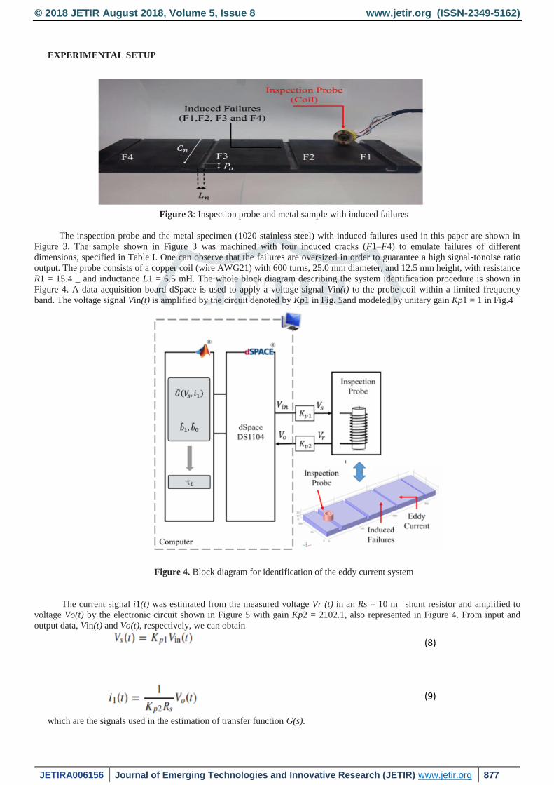
R1 = 15.4 _ and inductance L1 = 6.5 mH. The whole block diagram describing the system identification procedure is shown in

Figure 4. A data acquisition board dSpace is used to apply a voltage signal Vin(t) to the probe coil within a limited frequency

band. The voltage signal Vin(t) is amplified by the circuit denoted by Kp1 in Fig. 5and modeled by unitary gain Kp1 = 1 in Fig.4

Figure 4. Block diagram for identification of the eddy current system

The current signal i1(t) was estimated from the measured voltage Vr (t) in an Rs = 10 m_ shunt resistor and amplified to

voltage Vo(t) by the electronic circuit shown in Figure 5 with gain Kp2 = 2102.1, also represented in Figure 4. From input and

output data, Vin(t) and Vo(t), respectively, we can obtain

which are the signals used in the estimation of transfer function G(s).

(8)

(9)




SYSTEM IDENTIFICATION

System identification tools can be used in order to characterize the presented eddy current system. Because the mathematical

model (6) is a function of the sample parameters (M, L2, and R2), it is expected that different failures produce variations in these

parameters. The applied voltage signal Vs(t), ranging from 100 to 3500 Hz [25], is sufficiently rich in frequencies that allow the

eddy current flow to take alternate paths.A signal u(k) is called sufficiently rich of order n if it contains at least (n/2) distinct

nonzero frequencies. By sampling signals Vs (t) and i1(t) at proper rate so that the Nyquist theorem is satisfied, a discrete model

G(z, θ) can be identified through prediction error identification. The chosen model class to be

identified is given by

i1(k, θ) = G(z, θ)Vs(k) + H(z, θ)e(k)

where ,

k = nT , T being the sampling period and n an integer

G(z, θ) is the process discrete-time transfer function,

H(z, θ)is the noise filter

e(k) is white noise with zero mean and variance σ2

Because (6) is second order, the process discrete-time model to be identified is given by

G(z, θ) = θ1z + θ2

z² + θ3z + θ4

The noise model can be chosen to minimize the variance of the estimate, though the estimate of G(z, θ) is unbiased because

data are collected in open loop

RESULTS

Eddy current Probe Identification

The probe was initially positioned over a portion of the sample without any visible fail. A pseudorandom binary sequence

(PRBS) signal was applied during 5 s, while the current i1(t) was measured. An illustration of the input PRBS and measured i1(t)

signals (time interval of 0.1 s) is shown in Figure 6. Even though the current signal presented in Figure 6 is given in milliamperes,

the identification of G(z, θ) was done using the international system of units, and the unit of G(z, θ )is amperes/volt.Since the

model to be identified is supposed to have a relation with the continuous model, the parameters of which are related to circuit

parameters, the process model structure to be identified is the one given in (10). However, the noise model H(z, θ) needs to be

chosen. The better this structure represents the noise, the smaller will be the variance of G(z, θ) parameters. Any noise model

structure could have been chosen, because the noise level is not high, as can be seen in Figure 6. An autoregressive moving

average with exogeneous input structure was chosen, where G(z, θ) is given by (10) and

H(z, θ) = z² + θ5 z + θ6

z² + θ3 z + θ4

to ease a future online identification implementation. In this seminar,the MATLAB ident toolbox was used in the

identification procedure.The experimental procedure was repeated 50 times in order to identify the reference transfer function

GF0 (s), as well as the standard deviation of its parameters.Thus, the probe was placed in the center of each of the induced

failures F1–F4. Again, the procedure was repeated 50 times, identifying the transfer function on each failure.

Figure 6:PRBS excitation signal Vs(t) and measured current i1(t)

The average values of the model parameters (as well as the standard deviation) at each failure position can be seen in Table

I, where they are organized from the transfer function representing the largest failure, GF1 , to the transfer function representing

no failure, GF0 . Note that the mean parameters of GF0 are significantly different from the ones obtained with different failures.

(10)




The identified parameters of the transfer function on each induced failure of the specimen were normalized in relation to the

parameters of GF0 (s) (no failure). Figure 6 shows the normalized results and the variations of the parameters to the four induced

failures F1–F4. It can be seen that the variations due to the failures are higher than the ones due to random interferences, showing

measurement repeatability.

Figure 7:Estimated inductive time constant τL in each induced failure of the specimen

Inductive Time Constant τL Estimation

From (7), the inductive time constant was calculated for each of the transfer functions GF0 (s), GF1 (s), GF2 (s), GF3

(s), and GF4 (s), representing no failure and the induced failures. The average values with standard deviation are shown in Figure

7. The larger the failure is, the greater the estimated ˆ τL value is. Also, the relative variation of the time constant (in the available

specimen) ranges from approximately 2.92% to greater variation 5.62% compared with the time constant obtained in the piece

with no failure. The bars at the average point represent the standard deviation of the measured data (very low variability). Figure 7

shows that the probe is sufficiently sensitive to the smallest failure (in the used sample), but not very sensitive to detect the

differences between the larger failures. This is a characteristic of the used probe. By modifying the probe and identifying the new

transfer function, the results will be associated with this new probe measuring a sample. Thus, the results illustrated in Figure 7

represent the results of the presented method (illustrated by the inductive constant time τL ) applied on the probe used to measure

the sample of Fig. 2.Although the induced failures of the sample are not small as in real applications of ECM and the probe is not

very sensitive (such as a differential probe, for instance), they can be used to evaluate the presented method and compare it with

the impedance classical method because the same probe and sample are used to measure both the impedance and the transfer

function parameters. We can expect that by changing the probe, the sample, or both, new parameters of the transfer function will

be produced, as a new reflected impedance.

Comparison With the Equivalent Impedance Analysis

The equivalent impedance of each failure can be calculated with the identified transfer function of each failure by

considering

s = jω

Zeq( jω) = 1

G( jω)

= Vs ( jω)

i1( jω)

Thus, the impedance in the five positions of the probe can be calculated using the estimates of the transfer functions GF0 (s)–

GF4 (s).

The relative variation of the reflected impedance from failures F0 and F1 was approximately 4.61% (at 1 kHz). The relative

change of the inductive time constant τL to the same failures is about 5.62%. While the time constant of the sample τL depends

only on the physical equivalent parameters of the sample represented by R2 and L2, the reflected impedance Zeq depends on the

mutual inductance M (and hence the coupling factor k and the distance between the probe and the

sample) in addition to the excitation frequency ω. Considering the distance between the sample surface and the probe fixed,

we can state that the equivalent impedance depends on the dimensions of the failures and the applied frequency. Figure 8

illustrates the result of the equivalent impedance obtained to the probe moving to each induced failure with frequency ranging

from 0 to 1 kHz. From the result, it can be inferred that for higher frequencies, this method is able to recognize different failures,

but this is not true for lower frequencies. The probe excitation frequency is usually chosen according to the application. Low

frequencies allow eddy currents to penetrate the sample. On the other hand, high frequencies are used for surface analysis of the

sample. The following expression describing the penetration depth (δ) dependent of frequency is usually used

(15)




Where,

μ is the sample magnetic permeability and σ is the electrical conductivity.

Figure 8 also shows that the variation of the equivalent impedance decreases at low frequencies, making detection very

difficult to any failure. A comparison of the percentage variation of the equivalent impedance Zeq when the probe is moved from

failure F0 to F1 with the percentage variation of the time constant τL can be seen in Table III.Note that the normalized variation

of the equivalent impedance increases with increasing frequency, while the normalized variation of the estimated time constant is

not a function of the frequency, and is still higher than the impedance variation obtained with the highest frequency tested, 1 kHz.

Figure 8:Impedence Zeq calculated with the transfer function with frequency ranging from 0 Hz to 1 kHz

CONCLUSION

This paper presented the analysis of a novel ECT system for detection of failures in conductive materials based on the

identification of an equivalent transfer function. Instead of assessing the variation of impedance when the probe is scanning a

metal sample, the variations of the identified parameters of the transfer function were monitored. A metal sample was machined

with grooves emulating failures. An inductive probe and a conditioning electronic circuit were built in order to apply a limited

band excitation signal to the sample and for monitoring variations of both current and voltage signals.The identification of the

parameters of an equivalent transfer function allowed the determination of the equivalent inductive time constant of the sample

being analyzed, which has the advantage of being frequency and mutual inductance independent. Moreover, an FEM software

was used to estimate the value of mutual inductance and consequently of other unknown circuit components, which were used to

validate the experimental results through the sensitivity analysis of the time constant identification compared with the impedance

estimation. The sensitivities of the two methods were calculated and compared. Finally,the use of a mathematical model to

describe the process of eddy currents results in an increment of information to the user. The presented approach can be used to

either measure the impedance variation or analyze each transfer function parameter, such as τL , explored here. Thus, an eddy

current measurement system based on usual probes with minor design modifications and the inclusion of a signal processing box

can produce more information from the sample under test. The continuation of this work will investigate the advantages presented

by the technique in real applications, by testing smaller and near real defects, different materials, as well the non idealities of the

system and non modeled phenomena suchas intrinsic capacitances of the probes.

REFERENCES

[1] Analytical Model for Tilted Coils in Eddy-Current Nondestructive Inspection Theodoros Theodoulidis, Member, IEEE Energy

Department, West Macedonia University, Kozani 50100, Greece

[2] Characterization of an Eddy-Current-Based System for Nondestructive Testing- Andrea Bernieri, Giovanni Betta, Senior

Member, IEEE, and Luigi Ferrigno

[3] Impedance of the Eddy-Current Displacement Probe: The Transformer Model Darko Vyroubal, Member, IEEE

[4] Crack Depth Estimation by Using a Multi-Frequency ECT Method Andrea Bernieri, Giovanni Betta, Senior Member, IEEE,

Luigi Ferrigno, Member, IEEE, and Marco Laracca, Member, IEEE.

[5] L. Li, “Eddy-current displacement sensing using switching drive where baseband sensor output is readily available,” IEEE

Trans. Instrum. Meas., vol. 57, no. 11, pp. 2548–2553, Nov. 2008.

[6 ]Non-Destructive Techniques Based on Eddy Current Testing -Javier Garcia Martin,Jaime Gómez Gil, and Ernesto Vázquez-

Sánchez .


Documents

EVALUATION OF METAL CRACKS USING EDDY CURRENT …