Evaluation of Noble Gas Recharge Temperatures ina Shallow Unconfined Aquiferby Bradley D. Cey1, G. Bryant Hudson2, Jean E. Moran3, and Bridget R. Scanlon4

AbstractWater table temperatures inferred from dissolved noble gas concentrations (noble gas temperatures, NGT) are

useful as a quantitative proxy for air temperature change since the last glacial maximum. Despite their importancein paleoclimate research, few studies have investigated the relationship between NGT and actual recharge temper-atures in field settings. This study presents dissolved noble gas data from a shallow unconfined aquifer heavilyimpacted by agriculture. Considering samples unaffected by degassing, NGT calculated from common physicallybased interpretive gas dissolution models that correct measured noble gas concentrations for ‘‘excess air’’ agreedwith measured water table temperatures (WTT). The ability to fit data to multiple interpretive models indicatesthat model goodness-of-fit does not necessarily mean that the model reflects actual gas dissolution processes.Although NGT are useful in that they reflect WTT, caution is recommended when using these interpretive models.There was no measurable difference in excess air characteristics (amount and degree of fractionation) betweentwo recharge regimes studied (higher flux recharge primarily during spring and summer vs. continuous, low fluxrecharge). Approximately 20% of samples had dissolved gas concentrations below equilibrium concentration withrespect to atmospheric pressure, indicating degassing. Geochemical and dissolved gas data indicate that saturatedzone denitrification caused degassing by gas stripping. Modeling indicates that minor degassing (,10% �Ne)may cause underestimation of ground water recharge temperature by up to 2�C. Such errors are proble-matic because degassing may not be apparent and degassed samples may be fit by a model with a high degreeof certainty.

IntroductionDissolved noble gases (He, Ne, Ar, Kr, and Xe) pro-

vide unique and valuable information in hydrologic stud-ies. The conservative behavior of noble gases allows

estimation of water table temperatures at the time ofground water recharge (noble gas temperatures, NGT) aswell as ground water ages. NGT are particularly impor-tant in paleoclimate research for quantifying the tempera-ture difference from the last glacial maximum (LGM, 23to 18 ka BP) to present (e.g., Farrera et al. 1999). NGTare also used in studies to quantify mountain front/blockrecharge (e.g., Manning and Solomon 2005).

It is common for ground water to contain dissolvedgas concentrations greater than equilibrium concentrationwith respect to atmospheric pressure. The additional dis-solved gas is termed ‘‘excess air’’ because of its composi-tional similarity to air (Heaton and Vogel 1981). Somesuggest that excess air may itself be a valuable paleo-climate proxy (Aeschbach-Hertig et al. 2002a; Castroet al. 2007).

NGT are much more sensitive to concentrations ofheavier gases (e.g., Xe, Kr) because the solubility ofthese gases have much greater temperature dependency.

1Corresponding author: Department of Geological Sciences,Jackson School of Geosciences, University of Texas at Austin, 1University Station C1100, Austin, TX 78712-0254; (512) 471-5172;fax (512) 471-9425; cey.home@gmail.com

2Chemical Sciences Division, Lawrence Livermore NationalLaboratory, Livermore, CA 94550

3Department of Earth and Environmental Sciences, CaliforniaState University, East Bay, Hayward, CA 94542

4Bureau of Economic Geology, Jackson School of Geo-sciences, University of Texas at Austin, Austin, TX 78712

Received May 2008, accepted February 2009.Copyright ª 2009 The Author(s)Journal compilationª2009NationalGroundWater Association.doi: 10.1111/j.1745-6584.2009.00562.x

646 Vol. 47, No. 5–GROUND WATER–September-October 2009 (pages 646–659) NGWA.org

In contrast, excess air is much more sensitive to concen-trations of lighter gases (e.g., He, Ne) because lightergases are only sparingly soluble (therefore additional dis-solved gas causes a large relative change). Accuratedetermination of excess air is necessary for ground waterage-dating using the 3H–3He technique (Solomon andCook 2000). It is common to measure multiple gases tocalculate NGT and excess air simultaneously using anerror weighted inverse modeling procedure (Aeschbach-Hertig et al. 1999, 2000).

Despite the importance of NGT in paleoclimateresearch, few studies have attempted to experimentallyconfirm that NGT accurately reflect water table tempera-tures (WTT). This deficiency is critical given recent workexamining assumptions in NGT calculations (Castro et al.2007; Hall et al. 2005). Most noble gas studies reportmean annual air temperature (MAAT) and the sampledwater temperature. Because sampled wells are rarelyscreened across the water table, the sampled water tem-perature represents aquifer temperatures but not necessar-ily WTT. It is extremely rare for researchers to directlymeasure WTT in noble gas studies.

Holocher et al. (2002) completed a series of laboratorycolumn experiments in which excess air was generated.The NGT matched the column temperature within mea-surement uncertainty for all samples. Stute and Sonntag(1992) investigated the relationship between NGT and sub-surface temperature. NGT at a site near Bocholt, Germany,showed evidence of recharge from two areas (i.e., forestand field/meadow) having different soil thermal regimes.Subsurface temperature data from ~1 m above the watertable were available from a nearby meteorological stationhaving field/meadow vegetation. No temperature measure-ments for the forested area were reported. The NGT ofground water recharged in the field/meadow was the sameas the measured soil temperature.

In a regional study, Castro et al. (2007) comparedcalculated NGT to recharge zone ground water temper-atures. Although unable to match NGT to ground watertemperature using common gas dissolution models, theNGT results matched ground water temperature if sub-surface noble gas partial pressures were assumed to begreater than their respective atmospheric partial pressures.Subsurface noble gas partial pressures could be elevatedrelative to atmospheric conditions from O2 consumptionby biological processes and subsequent dissolution of theproduced CO2 (Stute and Schlosser 2000).

Klump et al. (2007) reported on field-scale noble gasdissolution experiments from two sites. In situ temper-atures were not taken at the two study sites; however, sub-surface temperatures were inferred from either measuringsamples of recently recharged water or using data froma nearby (~20 km) meteorological station. They con-cluded that calculated NGT accurately reflected in situsoil temperatures.

In each of these three field studies, subsurface tem-perature data were considered in an attempt to compareNGT to WTT. However, none of these studies incorpo-rated direct measurements of subsurface temperature to

examine the relationship between NGT of very young(weeks to years) ground water to WTT.

The objectives of this study were to (1) comparemodeled NGT to measured WTT to evaluate potentialbias in NGT, (2) compare differences in gas dissolutionoccurring under two different recharge regimes (higherflux recharge primarily during spring and summer vs.continuous, low flux recharge), and (3) examine thepotential impact of degassing on NGT. Improved under-standing of gas dissolution processes occurring duringground water recharge will benefit ground water age-dating and paleoclimate studies. This study offers the fol-lowing improvements over the noble gas studies dis-cussed: (1) high frequency measurements of subsurfacetemperature throughout the unsaturated zone at multiplelocations, (2) noble gas concentrations measured at multi-ple locations across the site, and (3) two differentrecharge regimes. This study complements recent workfrom the same site by Singleton et al. (2007) that focusedon evidence for saturated zone denitrification and byMcNab et al. (2007) that focused on the geochemistry ofmanure lagoon water. Singleton et al. (2007) present onlyaverages of NGT and excess air for the site and calculateNGT using only Xe data. All analyses of dissolved noblegas data presented in this study are original—revised andexpanded from the previous analyses by Singleton et al.(2007).

Materials and Methods

Study SiteThe study site includes a dairy farm and surrounding

fields in Kings County, California. The climate is Medi-terranean type with hot summers and mild winters(MAAT ¼ 16.6�C). Mean annual precipitation is 170 mm,with 80% falling during the coolest 5 months (Novemberthrough March). Local meteorological data were obtainedfrom a nearby (~10 km) National Climatic Data Center(NCDC) station. The site has minimal topographic relief(,2 m) and an elevation ~70 m above mean sea level.The local geology consists of unconsolidated sediments(primarily sands and silts) that were deposited in a seriesof alluvial fan systems originating where rivers exit theSierra Nevada (Weissmann et al. 1999).

Cropland surrounding the dairy operation is floodirrigated with a combination of ground water and dairywastewater (i.e., liquid manure). Occasionally water fromthe Kings River is transported through unlined canals forirrigation. Ground water used for irrigation is drawn fromboth a shallow perched aquifer (�25 m below groundsurface, bgs) and a deeper aquifer (�40 m bgs). Anunsaturated zone separates these two aquifers. Water fordomestic use is drawn from the deep aquifer. The watertable is ~5 m bgs across the site. Ground water flowdirection within the perched aquifer is difficult to charac-terize because of many irrigation wells that pump inter-mittently and seasonally filled irrigation canals. Deeperregional ground water flow is generally westward toward

NGWA.org B.D. Cey et al. GROUND WATER 47, no. 5: 646–659 647

the center of the valley (Williamson et al. 1989). Addi-tional details of the study site are given in McNab et al.(2007) and Singleton et al. (2007).

Five sets (locations 1S, 2S, 3S, 4S, and 6S) of smalldiameter multilevel wells were installed at the site (loca-tions are given in Figure 1, depths are given in Table 1)as part of related studies (McNab et al. 2007; Singletonet al. 2007). These multilevel well sites are all located onthe edges of flood irrigated fields alternatingly plantedwith corn and wheat, except 2S, which is beside an alfalfafield, and 6S, which is between cattle pens and manure la-goons. A sixth single completion well site (well 5S1) islocated in a field ~11 m from the study area’s main irriga-tion canal. This 14-m-wide canal is commonly full onlyduring spring and summer months. All wells were 5 cmdiameter, except 6S wells, which were 2.5 cm diameter.Screen lengths for these wells were 61 cm.

At three of the six well locations, additional unsatu-rated zone instrumentation was installed in February2005. The three instrumented sites span the range ofrecharge conditions at the site: focused, higher fluxrecharge from irrigation canal leakage at 5S (rechargeoccurs during spring and summer only), and lower flux,relatively uniform recharge at 2S and 3S caused by regu-lar flood irrigation. The 2S wells are away from irrigationwells, and 3S wells are between two irrigations wells(~25 and ~40 m away) that cause recurrent, local watertable fluctuations. The instrumentation was placed atmultiple depths in hand-augured boreholes to span theentire unsaturated zone at each location. Each boreholewas instrumented with multiple sensors to record hourly

measurements of soil temperature and matric potential(heat dissipation sensor model 229-L, Campbell Scien-tific Inc., Logan, Utah) and soil gas pressure (Druckbarometer model RPT410F, Campbell Scientific Inc.).The approximate depths of heat dissipation sensors ateach instrumented location were 0.4, 0.6, 0.9, 1.5, 2.4,and 3.9 m BGS. Before installation, heat dissipation sen-sors were calibrated using both pressure plate extractorsand salt solutions (Scanlon et al. 2005).

Ground water samples were collected from multi-level wells using a portable, submersible pump(GrundfosTM), with the exception of the smaller diameter6S wells, which were sampled using a bladder pump.Ground water samples from multilevel wells were ana-lyzed for pH in the field using a Horiba U-22 water qual-ity meter. Cation and anion concentrations were measuredby ion chromatography using a Dionex DX-600. Oxygenisotopic composition of water was measured using thecarbon dioxide equilibration method for 18O/16O (Epsteinand Mayeda 1953) on a VG Prism II isotope massspectrometer.

Samples for dissolved noble gas analyses were col-lected in copper tubing sample vessels (8 mm inner dia-meter, 250 mm long). Steel clamps pinched the coppertubing flat in two locations to secure the water sample.Dissolved noble gas concentrations were measured asdescribed in Cey et al. (2008). Analytical uncertaintiesare approximately 2% for He, Ne, and Ar and 3% for Krand Xe.

All laboratory analyses of ground water samples werecompleted at Lawrence Livermore National Laboratory. The

Figure 1. Map of study site. Only the sampled irrigation wells are uniquely labeled. Irrigation wells owned by other land-owners are not shown.

648 B.D. Cey et al. GROUND WATER 47, no. 5: 646–659 NGWA.org

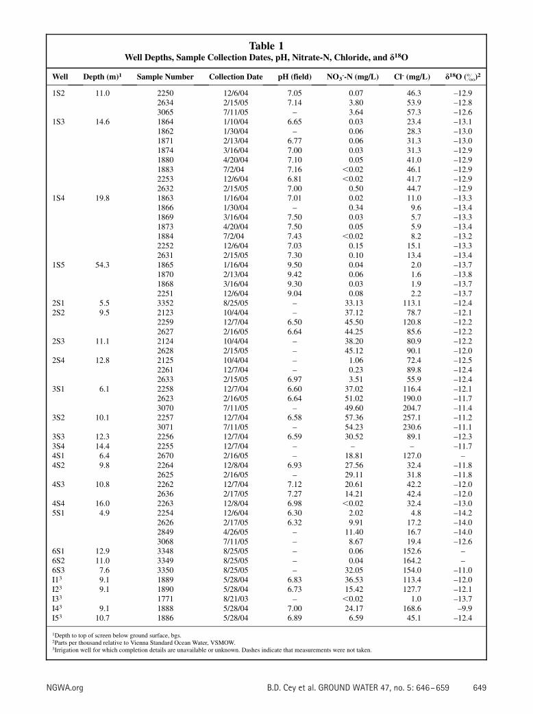
Table 1Well Depths, Sample Collection Dates, pH, Nitrate-N, Chloride, and d18O

Well Depth (m)1 Sample Number Collection Date pH (field) NO3--N (mg/L) Cl- (mg/L) d18O (&)2

1S2 11.0 2250 12/6/04 7.05 0.07 46.3 –12.92634 2/15/05 7.14 3.80 53.9 –12.83065 7/11/05 – 3.64 57.3 –12.6

1S3 14.6 1864 1/10/04 6.65 0.03 23.4 –13.11862 1/30/04 – 0.06 28.3 –13.01871 2/13/04 6.77 0.06 31.3 –13.01874 3/16/04 7.00 0.03 31.3 –12.91880 4/20/04 7.10 0.05 41.0 –12.91883 7/2/04 7.16 ,0.02 46.1 –12.92253 12/6/04 6.81 ,0.02 41.7 –12.92632 2/15/05 7.00 0.50 44.7 –12.9

1S4 19.8 1863 1/16/04 7.01 0.02 11.0 –13.31866 1/30/04 – 0.34 9.6 –13.41869 3/16/04 7.50 0.03 5.7 –13.31873 4/20/04 7.50 0.05 5.9 –13.41884 7/2/04 7.43 ,0.02 8.2 –13.22252 12/6/04 7.03 0.15 15.1 –13.32631 2/15/05 7.30 0.10 13.4 –13.4

1S5 54.3 1865 1/16/04 9.50 0.04 2.0 –13.71870 2/13/04 9.42 0.06 1.6 –13.81868 3/16/04 9.30 0.03 1.9 –13.72251 12/6/04 9.04 0.08 2.2 –13.7

2S1 5.5 3352 8/25/05 – 33.13 113.1 –12.42S2 9.5 2123 10/4/04 – 37.12 78.7 –12.1

2259 12/7/04 6.50 45.50 120.8 –12.22627 2/16/05 6.64 44.25 85.6 –12.2

2S3 11.1 2124 10/4/04 – 38.20 80.9 –12.22628 2/15/05 – 45.12 90.1 –12.0

2S4 12.8 2125 10/4/04 – 1.06 72.4 –12.52261 12/7/04 – 0.23 89.8 –12.42633 2/15/05 6.97 3.51 55.9 –12.4

3S1 6.1 2258 12/7/04 6.60 37.02 116.4 –12.12623 2/16/05 6.64 51.02 190.0 –11.73070 7/11/05 – 49.60 204.7 –11.4

3S2 10.1 2257 12/7/04 6.58 57.36 257.1 –11.23071 7/11/05 – 54.23 230.6 –11.1

3S3 12.3 2256 12/7/04 6.59 30.52 89.1 –12.33S4 14.4 2255 12/7/04 – – – –11.74S1 6.4 2670 2/16/05 – 18.81 127.0 –4S2 9.8 2264 12/8/04 6.93 27.56 32.4 –11.8

2625 2/16/05 – 29.11 31.8 –11.84S3 10.8 2262 12/7/04 7.12 20.61 42.2 –12.0

2636 2/17/05 7.27 14.21 42.4 –12.04S4 16.0 2263 12/8/04 6.98 ,0.02 32.4 –13.05S1 4.9 2254 12/6/04 6.30 2.02 4.8 –14.2

2626 2/17/05 6.32 9.91 17.2 –14.02849 4/26/05 – 11.40 16.7 –14.03068 7/11/05 – 8.67 19.4 –12.6

6S1 12.9 3348 8/25/05 – 0.06 152.6 –6S2 11.0 3349 8/25/05 – 0.04 164.2 –6S3 7.6 3350 8/25/05 – 32.05 154.0 –11.0I13 9.1 1889 5/28/04 6.83 36.53 113.4 –12.0I23 9.1 1890 5/28/04 6.73 15.42 127.7 –12.1I33 1771 8/21/03 – ,0.02 1.0 –13.7I43 9.1 1888 5/28/04 7.00 24.17 168.6 –9.9I53 10.7 1886 5/28/04 6.89 6.59 45.1 –12.4

1Depth to top of screen below ground surface, bgs.2Parts per thousand relative to Vienna Standard Ocean Water, VSMOW.3Irrigation well for which completion details are unavailable or unknown. Dashes indicate that measurements were not taken.

NGWA.org B.D. Cey et al. GROUND WATER 47, no. 5: 646–659 649

pH, chloride, and 18O data presented here were previouslyreported by McNab et al. (2007), except for 18O of lagoonwater. The nitrate and dissolved noble gas data presentedhere were previously reported by Singleton et al. (2007).

Noble Gas ModelingThe equilibrium concentration, Ci,eq, of gas i is given

by Henry’s law as:

Ci;eq ¼pi

HiðT; SÞð1Þ

where pi is partial pressure of gas i and Hi is Henry’s lawconstant, which is a function of temperature T and salinityS. The total measured concentration, Ci, of dissolved gas iis the sum of multiple components:

Ci ¼ Ci;eq 1 Ci;exc 1 Ci;rad 1 Ci;ter ð2Þ

where subscripts exc, rad, and ter refer to excess air, radio-genic, and terrigenic components, respectively.

Helium is commonly excluded from noble gas mod-eling because of complications that arise from the pres-ence of radiogenic sources such as tritiogenic 3He(Solomon and Cook 2000) or 4He from U and Th decay(Solomon 2000). Calculation of equilibrium and excessair components of He is required to quantify tritiogenic3He, which is used to calculate 3H–3He ground water ages(Solomon and Cook 2000). Singleton et al. (2007) foundonly young (,50 years) ground water in the perchedaquifer, which suggests negligible radiogenic componentsof 4He, Ne, Ar, Kr, and Xe. It was assumed that 4He, Ne,Ar, Kr, and Xe did not have significant radiogenic or ter-rigenic components in the study area (Lehmann et al.1993); however, the deeper aquifer (well 1S5) may containradiogenic 4He.

Three physically based models are commonly usedto interpret dissolved noble gas concentration datain ground water: (1) unfractionated air (UA) model(Heaton and Vogel 1981), (2) partial reequilibration(PR) model (Stute et al. 1995), and (3) closed systemequilibrium (CE) model (Aeschbach-Hertig et al. 2000).The UA model is the simplest because it assumes theexcess air component is atmospheric air resulting fromcomplete dissolution of entrapped air bubbles duringrecharge. The total concentration of gas i as given by theUA model is:

CUAi ¼ Ci;eq 1 Ad � zi ð3Þ

where Ad is concentration of dry air dissolved and zi isvolume fraction of gas i in dry air. Stute et al. (1995) pos-tulated elemental fractionation in the excess air compo-nent (whereby lighter gases are depleted relative toheavier gases) and suggested that this fractionation wascaused by complete bubble dissolution followed by diffu-sive degassing (PR model). The total concentration of gasi as given by the PR model is:

CPRi ¼ Ci;eq 1 ðAd � ziÞ � e

�RPR �DiDNe ð4Þ

where Ad is initial concentration of dissolved excess air,RPR is degree of reequilibration, Di is molecular diffusiv-ity of gas i, and DNe is molecular diffusivity of Ne. Kipferet al. (2002) extended the PR model to include multipledissolution-degassing cycles. Aeschbach-Hertig et al.(2000) suggested that fractionation of excess air resultsfrom incomplete dissolution of entrapped air bubbles andfractionation is related to differing gas solubilities (CEmodel). The total concentration of gas i as given by theCE model is:

CCEi ¼ Ci;eq 1

ð1� FÞ � Ae � zi1 1

�F�Ae�ziCi;eq

� ð5Þ

where F is a fractionation parameter and Ae is initial con-centration of entrapped air:

Ae ¼V0g

qðT; SÞ � Vw��Pg � es

�P0

ð6Þ

where Vg0 is initial volume of entrapped air, q is water

density as a function of temperature T and salinity S, Vw isvolume of water, Pg is pressure of entrapped air, es is sat-uration water vapor pressure, and P0 is standard pressure(1 atm). The fractionation parameter is:

F ¼ v

q¼

�Vg

V0g

��

Pg�esPatm�es

� ð7Þ

where Vg is volume of entrapped air, Patm is atmosphericpressure, v is fraction of entrapped air remaining, and q isthe ratio of dry entrapped air pressure to dry atmosphericpressure (which is approximately the pressure on the en-trapped air).

The UA model is a limiting case for both the CEmodel (when F ¼ 0) and the PR model (when RPR ¼ 0).CE and PR models can give similar results becauseunderlying physical processes for these two models varysimilarly among gases. Peeters et al. (2002) suggestedthat in addition to noble gas concentration data, isotopicdata—especially Ne—are helpful in distinguishing be-tween diffusive degassing (PR model) and incompletebubble dissolution (CE model).

Addition of excess air has the greatest relative impacton He and Ne concentrations because the equilibriumcomponent is relatively small. A common way to repre-sent the amount of excess air is as percent Ne, �Ne(Kipfer et al. 2002):

�Ne ¼ CNe;exc

CNe;eq3 100% ð8Þ

Dissolved gas concentrations may be reduced by de-gassing after recharge. Just as gas dissolution models arebased on solubility (CE model) and diffusion (PR model),degassing can be controlled by solubility or diffusion.Such degassing occurs as a result of the formation of ini-tially noble gas free gas bubbles (e.g., CO2, CH4, or N2).

650 B.D. Cey et al. GROUND WATER 47, no. 5: 646–659 NGWA.org

In the case of solubility controlled degassing occurring asa single step (DS1 model), the final degassed concentra-tion of gas i is:

CDS1i ¼ C�

i

1 1 B�ziC�i

ð9Þ

where Ci* is the initial (predegassing) concentration, B isa degassing parameter, and zi is the concentration of gas iin air. This model is comparable to the CE model, exceptthat the ‘‘entrapped air’’ of the CE model is free of noblegases in this case. This model was presented in Brennwaldet al. (2003) as the ‘‘one-step degassing model.’’ It can beextended to the case of repeated (continuous) gas bubbleformation/equilibration (DSC model). The final degassedconcentration is (equation 7 in Brennwald et al. [2005]):

CDSCi ¼ C�

i � e

��BziC�i

�ð10Þ

Alternatively, degassing may be controlled by gasdiffusion (DD model, Stute 1989). The final degassedconcentration is:

CDDi ¼ C�

i � e

��RDD Di

DNe

�ð11Þ

Diffusion controlled degassing is similar to the PRmodel; however, in this case, the dissolved gas diffusesinto a reservoir that is initially free of noble gases. Thelimiting case of RDD / N is therefore complete transferof all noble gases from the water to the gas phase. In con-trast, the limiting case of the PR dissolution model (whenRPR / N) results in minimum gas concentrations equiv-alent to the equilibrium concentration with respect toatmospheric pressure.

Measured dissolved noble gas concentrations weremodeled using NOBLE90, an error weighted, least-squares fitting, inverse modeling program (Aeschbach-Hertig et al. 1999; Peeters et al. 2002). NOBLE90 solvesfor parameter combinations for the selected interpretivemodel that match measured data within experimentalerror by minimizing v2, the sum of the weighted squareddeviations between the modeled and measured concen-trations. The ability of the selected model to describe theobserved data (i.e., goodness-of-fit of the selected model)is judged on the probability of v2 being greater than agiven value obtained from the v2 distribution (for the ap-propriate number of degrees of freedom). If this probability,p, is lower than a predetermined cutoff value, the solutionis rejected and it is concluded that the selected modelis unable to describe the measured data (Aeschbach-Hertig et al. 1999). This approach allows assessment ofthe likelihood that differences between modeled and mea-sured values result from experimental error. In this study,solutions with p , 0.05 are rejected. The gas solubilitydata used in the NOBLE90 calculations were from multi-ple sources (Clever 1979; Weiss 1970, 1971; Weiss andKyser 1978). Additional details of NOBLE90 are givenby Aeschbach-Hertig et al. (1999, 2000) and Peeters et al.(2002). Measured He, Ne, Ar, Kr, and Xe concentrations

were fitted by UA, PR, and CE models using NOBLE90to solve for excess air, degree of excess air fractionation(in CE and PR models only), and recharge temperature.Additional modeling using only measured Ne, Ar, Kr, andXe concentrations was also done. For all modeling, therecharging water was assumed to be fresh (S ¼ 0) andthe mean atmospheric pressure from the local NCDCmeteorological station was used.

Degassing of ground water after recharge impacts in-terpreted (modeled) values of recharge temperature andexcess air. Visser et al. (2007) examined the impact ofsaturated zone degassing on calculated 3H–3He ages, butdid not model NGT. Aeschbach-Hertig et al. (2008)reported success in modeling undersaturated groundwater samples from both the laboratory and a well usingsolubility-controlled degassing. To explore the impact ofdegassing on NGT, a separate modeling study was con-ducted. Hypothetical/synthetic dissolved noble gas datarepresentative of site ground water conditions (T ¼19.0�C, Patm ¼ 0.991 atm, S ¼ 0, �Ne ¼ 30%) weregenerated—both unfractionated (UA model) and frac-tionated according to the CE model (F ¼ 0.65 and 0.75).The representative gas concentrations were subsequentlydegassed by both the DS1 and DD models. The degree ofdegassing ranged from 0 to –10% �Ne. The degassedsamples were then modeled using the CE and UA models.

Results and Discussion

Soil-Gas PressureSoil-gas pressure data show pronounced diurnal and

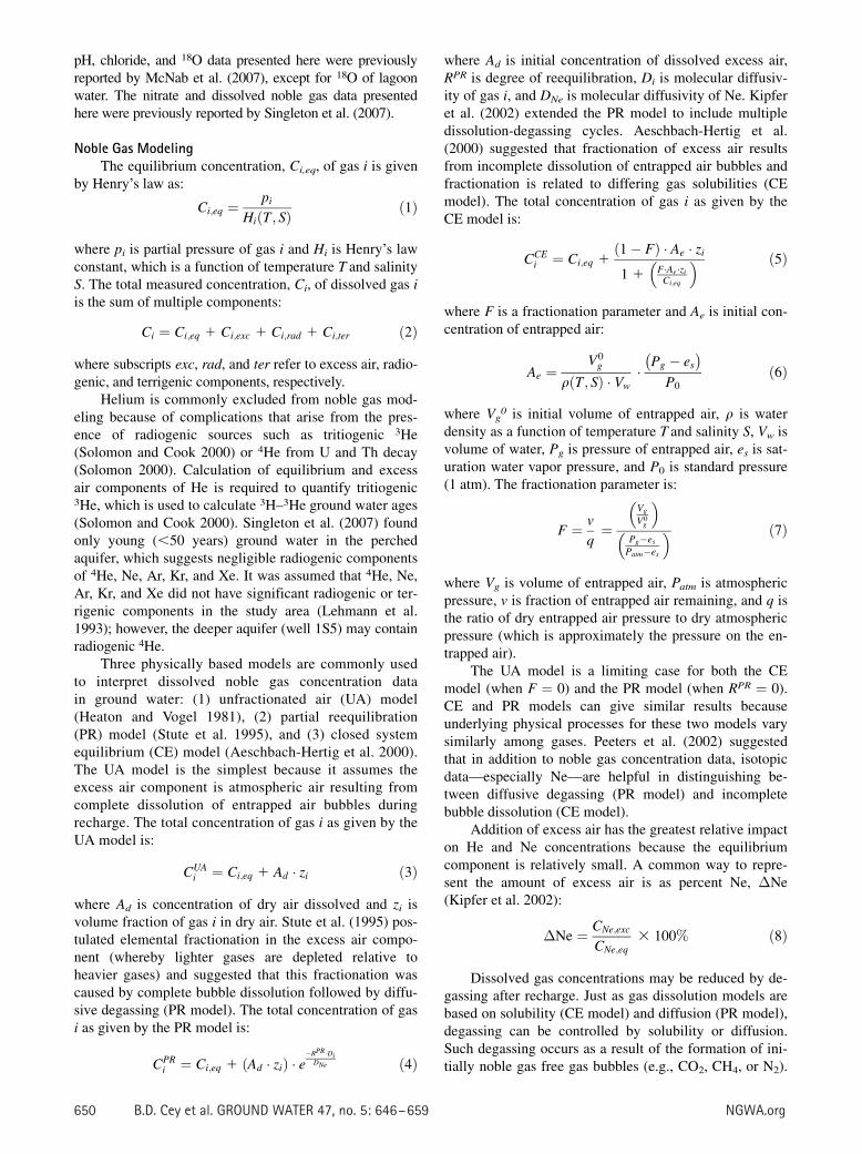
seasonal fluctuations (Figure 2). Atmospheric pressuredata from the nearby NCDC station closely track the

Figure 2. Atmospheric pressure data from nearby NationalClimatic Data Center (NCDC) station showing (a) seasonalfluctuations and (b) diurnal fluctuations. Panel (c) shows theimpact of the May 22, 2005, irrigation event at 2S on soil-gaspressure (site 2S sensors: gray; sites 3S and 5S: black).

NGWA.org B.D. Cey et al. GROUND WATER 47, no. 5: 646–659 651

measured soil-gas pressures, with few exceptions. Eachinstance of soil-gas pressures deviating from atmosphericpressures can be linked to irrigation events during whichsoil-gas pressure beneath the irrigated field increased~0.001 atm and subsequently dissipated in ,12 h(Figure 2c). No measurable pressure gradient was foundbetween the atmosphere and the unsaturated zone exceptduring irrigation events, and no measurable vertical pres-sure gradient existed within the unsaturated zone duringirrigation events.

Water TableHigh frequency measurements of water table depth

at all wells were not made. However, water table meas-urements made during sampling and matric potentialmeasurements indicate that the water table beneath irri-gated fields commonly rose by ~0.1 m in the days follow-ing an irrigation event. The annual water table rangebeneath irrigated fields was ~0.5 m. Because of its loca-tion between two irrigation wells, 3S responded differ-ently. The water table at 3S was drawn down ~1 m duringirrigation events.

When the irrigation canal adjacent to 5S1 was filled,there were small (,0.2 m) daily to weekly water tablefluctuations at 5S1, most likely caused by the fluctuationsin the canal’s water level. The water table at 5S1 waslowest during winter (canal empty) and had an annualrange ~1 m.

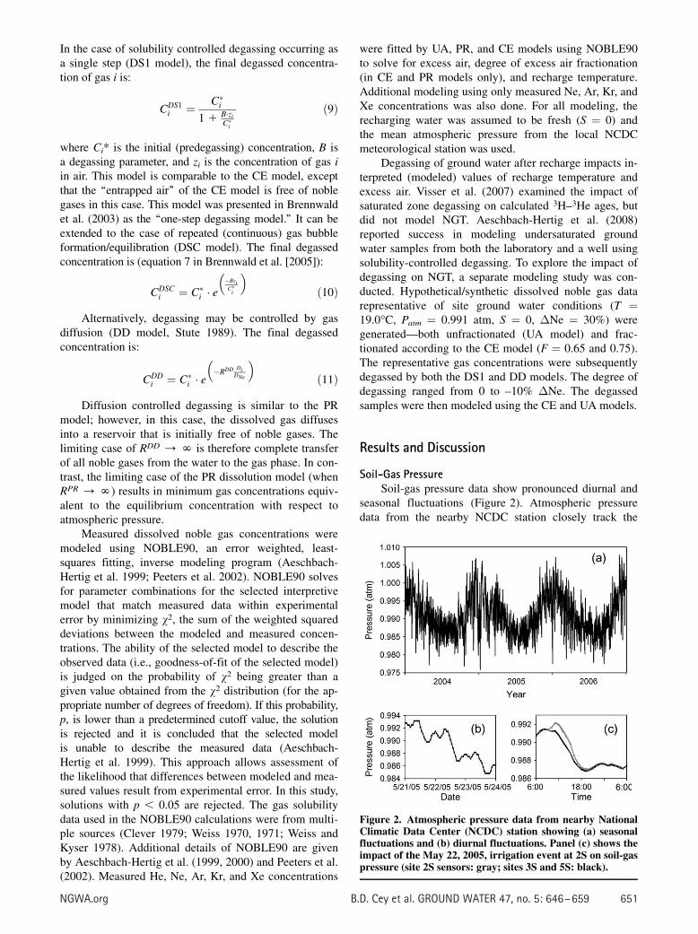
TemperatureMeasured subsurface temperature data show both the

lag and damping of seasonal temperature fluctuationswith increasing depth in the soil column (Figure 3).

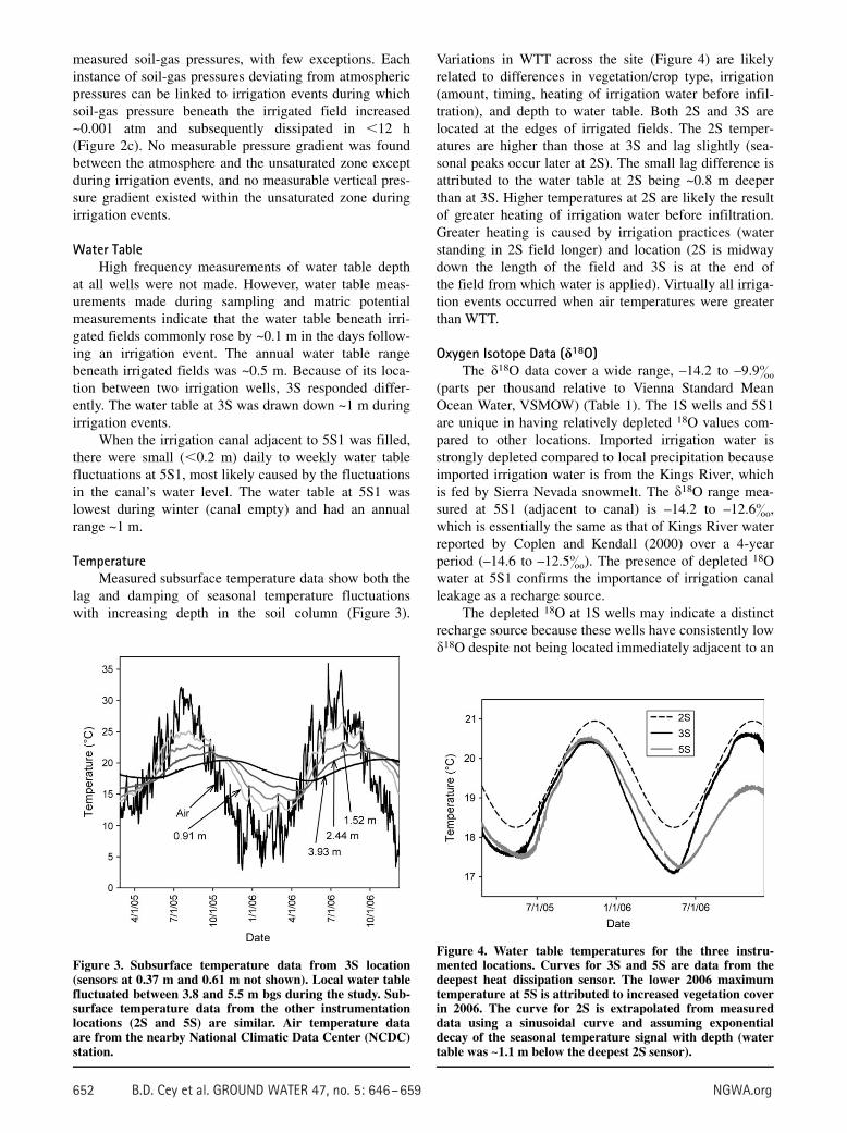
Variations in WTT across the site (Figure 4) are likelyrelated to differences in vegetation/crop type, irrigation(amount, timing, heating of irrigation water before infil-tration), and depth to water table. Both 2S and 3S arelocated at the edges of irrigated fields. The 2S temper-atures are higher than those at 3S and lag slightly (sea-sonal peaks occur later at 2S). The small lag difference isattributed to the water table at 2S being ~0.8 m deeperthan at 3S. Higher temperatures at 2S are likely the resultof greater heating of irrigation water before infiltration.Greater heating is caused by irrigation practices (waterstanding in 2S field longer) and location (2S is midwaydown the length of the field and 3S is at the end ofthe field from which water is applied). Virtually all irriga-tion events occurred when air temperatures were greaterthan WTT.

Oxygen Isotope Data (d18O)The d18O data cover a wide range, –14.2 to –9.9&

(parts per thousand relative to Vienna Standard MeanOcean Water, VSMOW) (Table 1). The 1S wells and 5S1are unique in having relatively depleted 18O values com-pared to other locations. Imported irrigation water isstrongly depleted compared to local precipitation becauseimported irrigation water is from the Kings River, whichis fed by Sierra Nevada snowmelt. The d18O range mea-sured at 5S1 (adjacent to canal) is –14.2 to –12.6&,which is essentially the same as that of Kings River waterreported by Coplen and Kendall (2000) over a 4-yearperiod (–14.6 to –12.5&). The presence of depleted 18Owater at 5S1 confirms the importance of irrigation canalleakage as a recharge source.

The depleted 18O at 1S wells may indicate a distinctrecharge source because these wells have consistently lowd18O despite not being located immediately adjacent to an

Figure 3. Subsurface temperature data from 3S location(sensors at 0.37 m and 0.61 m not shown). Local water tablefluctuated between 3.8 and 5.5 m bgs during the study. Sub-surface temperature data from the other instrumentationlocations (2S and 5S) are similar. Air temperature dataare from the nearby National Climatic Data Center (NCDC)station.

Figure 4. Water table temperatures for the three instru-mented locations. Curves for 3S and 5S are data from thedeepest heat dissipation sensor. The lower 2006 maximumtemperature at 5S is attributed to increased vegetation coverin 2006. The curve for 2S is extrapolated from measureddata using a sinusoidal curve and assuming exponentialdecay of the seasonal temperature signal with depth (watertable was ~1.1 m below the deepest 2S sensor).

652 B.D. Cey et al. GROUND WATER 47, no. 5: 646–659 NGWA.org

irrigation canal. The lack of variability of these samplesmay indicate a relative lack of mixing and therefore lessimpact by agricultural activity.

The most 18O enriched monitoring well sample was6S3 (–11.0&), the shallowest monitoring well within thedairy farm operations area. The enrichment at 6S3 islikely caused by evaporative enrichment of nearbymanure lagoon water (range –10.2 to –9.9&, n ¼ 4).Evaporative enrichment most likely occurs at manure la-goons as well as in the flood irrigated fields.

Repeated application of various different watertypes—shallow ground water, imported Kings Riverwater, and liquid manure—to fields limits the use of 18Oin this study. However, the 18O data verify the importanceof irrigation canal leakage as a source of recharge. Thesedata also suggest that imported water may be a significantcontributor to 1S recharge.

Dissolved Noble GasesDissolved noble gas data were collected between

August 2003 and August 2005 (Table 2). Analyses werecompleted on a number of duplicate samples. Someduplicate analyses did not reproduce initial results; how-ever, results from individual wells were generally compa-rable (,10% difference), if not within the statedanalytical uncertainty. The differences between duplicatesare most likely associated with sampling rather than withlaboratory analysis. Sampling ground water for dissolvedgases is challenging at shallow depths because of lowpore pressures. The differences in Kr and Xe between du-plicates were most often minimal (less than analyticalerror); therefore the impact on calculated NGT wasminimal.

Undersaturation

Several samples have gas concentrations below equi-librium gas solubility (e.g., samples from 1S2 and 2S4),indicative of degassing caused by gas stripping (i.e.,removal of dissolved noble gases from solution by parti-tioning into an initially noble gas free bubble). The lowmeasured gas concentrations are inconsistent withdecreased equilibrium concentrations caused by highsalinity, high temperature, or low pressure.

Many scenarios can result in ground water degassingby gas stripping. Denitrification-produced N2 is reported invarious studies to cause ground water degassing (Blicher-Mathiesen et al. 1998; Dunkle et al. 1993; Mookherji et al.2003; Visser et al. 2007). Strongly anoxic conditions canlead to gas stripping by exsolution of methane (Fortuin andWillemsen 2005; Puckett et al. 2002). Methane productionat hydrocarbon contaminated sites (Amos et al. 2005) andlandfills (Solomon et al. 1992) can also cause degassing.Recent laboratory studies confirm the ability of biogenicgases to strip other gases from solution (Amos and Mayer2006; Istok et al. 2007). Klump et al. (2006) reported slightundersaturation of dissolved gases in ground water andattributed it to gas stripping by CO2 or CH4 or both.

The location of subsurface gas production affectswhether or not degassing occurs. If gas production occurs

deep in the saturated zone, degassing is less likely tooccur because increased hydrostatic pressure at greaterdepths forces the produced gas to remain in solutionrather than form bubbles. However, if gas productionoccurs within a few meters of the water table, gas bubbleformation is more likely (Visser et al. 2007). Because themain sources of gas production tend to be reactions inanoxic conditions (e.g., denitrification and methano-genesis), the shallower the redox cline, the more favor-able it is for degassing to occur. The redox cline at thissite is ~11 m bgs, which is ~6 m below the water table(Singleton et al. 2007).

There is no evidence for methanogenesis occurring inthe shallow ground water; however, manure lagoon watersare methanogenic (McNab et al. 2007). McNab et al.(2007) suggested that observed Ar undersaturation in 2Ssamples is caused by CO2 or CH4 bubbles stripping pre-viously dissolved gases within manure lagoon water beforeits infiltration. However, this explanation cannot accountfor the undersaturated samples at wells farther from themanure lagoons (e.g., samples from 3S4 and 5S1).

Ample evidence for denitrification at the site exists,but the observed N2 excess caused by denitrification isless than expected for the observed nitrate concentrationdeclines (Singleton et al. 2007). As Singleton et al.(2007) suggest, the lack of mass balance may be theresult of N2 loss from the saturated zone, which wouldstrip noble gases from the ground water. Therefore, allsamples below the zone of denitrification (generally 11to 12 m bgs) may have undergone some degree of de-gassing. Such degassing may not be immediately notice-able if the initial excess air dissolved during recharge isgreater than the amount of gas lost during degassing, butthe interpreted recharge conditions could be inaccurateif degassing is not taken into account. Degassing bydenitrification may help explain the measured under-saturation at 1S and 2S.

Gas stripping may be controlled by gas solubility(Equations 9 and 10) or by diffusion (Equation 11). Thedifference in gas concentrations between the processes ismost relevant for light gases (i.e., He, Ne). The data sug-gest that solubility controlled degassing (DS1 and DSCmodels) occurs at 2S4 (Figure 5). There is also otherevidence (stable isotopes of dissolved inorganic carbon)indicating that 2S is impacted by manure lagoon recharge(McNab et al. 2007), suggesting that some 2S4 degassingoccurred within the manure lagoons before infiltration.There may be some diffusive degassing at other locations(e.g., 1S2); however, determination of the process causingdegassing would benefit from isotopic analyses (Peeterset al. 2002).

The two undersaturated samples from 5S1 occurredduring a time of little or no recharge (i.e., no irrigation inthe nearby field and the canal had been empty formonths). Samples from 5S1 taken when the canal wasfull were not undersaturated. There are no indications ofreducing conditions at 5S1. Low nitrate concentrationsare associated with low chloride (Table 1), indicating thedominance of low salinity recharge from the irrigation

NGWA.org B.D. Cey et al. GROUND WATER 47, no. 5: 646–659 653

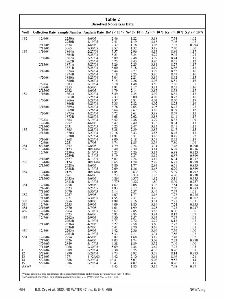
Table 2Dissolved Noble Gas Data

Well Collection Date Sample Number Analysis Date He1 (3 10-8) Ne1 (3 10-7) Ar1 (3 10-4) Kr1 (3 10-8) Xe1 (3 10-8)

1S2 12/6/04 2250A 4/6/05 2.46 1.22 3.18 7.54 1.022250B 4/19/05 2.41 1.19 3.18 7.46 1.08

2/15/05 2634 4/6/05 2.32 1.18 3.05 7.35 0.9947/11/05 3065 9/30/05 2.52 1.32 3.18 7.40 1.00

1S3 1/16/04 1864A 2/27/04 7.57 2.96 4.13 8.86 1.171864B 6/25/04 8.21 3.24 4.22 9.02 1.22

1/30/04 1862A 2/27/04 5.89 2.48 3.99 8.44 1.151862B 6/25/04 5.75 2.43 3.96 8.55 1.12

2/13/04 1871A 3/27/04 5.26 2.25 3.81 8.27 1.171871B 6/25/04 8.60 3.18 4.19 8.86 1.18

3/16/04 1874A 3/24/04 5.44 2.27 3.92 8.52 1.161874B 6/26/04 5.18 2.25 3.80 8.47 1.16

4/20/04 1880A 4/23/04 5.04 2.21 3.89 8.62 1.151880B 6/26/04 5.15 2.26 3.93 8.51 1.16

7/2/04 1883 8/19/04 3.10 1.48 3.50 7.86 1.0512/6/04 2253 4/5/05 4.91 2.17 3.81 8.65 1.162/15/05 2632 4/6/05 4.79 2.14 3.87 8.58 1.17

1S4 1/16/04 1863A 2/27/04 5.49 2.35 3.92 8.61 1.171863B 6/25/04 7.33 3.00 4.08 8.72 1.16

1/30/04 1866A 2/28/04 7.37 2.81 4.02 8.60 1.191866B 6/25/04 7.35 2.82 4.02 8.75 1.19

3/16/04 1869A 3/24/04 6.76 2.65 3.95 8.42 1.231869B 6/26/04 6.64 2.67 3.86 8.39 1.12

4/20/04 1873A 4/23/04 6.72 2.61 3.88 8.69 1.151873B 6/26/04 6.68 2.62 3.88 8.41 1.17

7/2/04 1884 8/19/04 6.52 2.46 3.79 8.33 1.0912/6/04 2252 4/6/05 6.42 2.49 3.75 8.34 1.132/15/05 2631 3/25/05 6.25 2.47 3.83 8.41 1.11

1S5 1/16/04 1865 2/28/04 5.38 2.39 3.87 8.47 1.152/13/04 1870A 2/27/04 12.16 3.43 3.85 8.45 1.17

1870B 3/27/04 11.91 3.31 3.86 8.45 1.223/16/04 1868 3/25/04 8.00 2.18 3.59 8.35 1.1912/6/04 2251 4/7/05 6.74 1.85 3.36 7.80 1.09

2S1 8/25/05 3352 9/8/05 4.79 2.24 3.34 7.48 0.9902S2 10/4/04 2123 10/14/04 5.49 2.39 3.14 6.88 0.916

12/7/04 2259A 2/10/05 5.25 2.26 3.13 6.88 0.9232259B 4/13/05 5.19 2.27 3.12 6.87 0.899

2/16/05 2627 4/13/05 5.07 2.24 3.12 6.94 0.9172S3 10/4/04 2124 10/14/04 3.65 1.78 2.99 6.77 0.879

2/15/05 2628A 4/6/05 3.80 1.77 2.94 6.61 0.8532628B 4/13/05 2.69 1.36 2.68 6.29 0.869

2S4 10/4/04 2125 10/14/04 1.85 0.638 1.99 5.39 0.79212/7/04 2261 4/6/05 0.735 0.314 1.76 4.90 0.7302/15/05 2633A 4/6/05 0.864 0.375 1.82 5.11 0.735

2633B 4/13/05 0.775 0.329 1.80 5.09 0.7573S1 12/7/04 2258 2/9/05 4.62 2.08 3.38 7.54 0.984

2/16/05 2623 3/25/05 4.93 2.12 3.45 7.60 0.9837/11/05 3070 9/30/05 5.14 2.37 3.46 7.67 1.01

3S2 12/7/04 2257 2/9/05 4.07 1.77 3.16 7.27 0.9757/11/05 3071 9/30/05 4.55 2.31 3.28 7.28 0.907

3S3 12/7/04 2256 2/9/05 4.99 2.16 3.54 7.91 1.033S4 12/7/04 2255 2/9/05 4.09 1.80 3.16 7.24 0.9554S1 2/16/05 2670 4/7/05 4.61 1.99 3.25 7.23 0.9474S2 12/8/04 2264 2/10/05 6.62 2.85 3.83 8.30 1.06

2/16/05 2625 4/6/05 6.85 2.85 3.84 8.12 1.074S3 12/7/04 2262A 2/9/05 6.30 2.57 3.67 7.97 1.04

2262B 4/19/05 6.77 2.72 3.72 8.12 1.032/17/05 2636A 4/7/05 6.22 2.58 3.60 7.72 1.01

2636B 4/7/05 6.41 2.70 3.65 7.77 1.014S4 12/8/04 2263A 2/9/05 4.42 2.36 3.66 7.59 1.00

2263B 4/19/05 5.33 2.11 3.34 7.56 1.025S1 12/6/04 2254 4/5/05 3.82 1.68 3.19 7.48 1.02

2/17/05 2626 4/6/05 4.03 1.74 3.09 7.23 0.9904/26/05 2849 5/17/05 4.38 1.89 3.32 7.49 1.007/11/05 3068 9/30/05 5.69 2.44 3.62 7.93 1.05

I1 5/28/04 1889 6/29/04 9.30 3.75 4.36 8.76 1.08I2 5/28/04 1890 6/29/04 7.73 2.92 3.79 8.14 0.993I3 8/21/03 1771 11/26/03 6.42 2.10 3.64 8.66 1.21I4 5/28/04 1888 6/29/04 13.4 5.07 5.03 9.57 1.14I5 5/28/04 1886 6/29/04 10.4 4.02 4.40 8.76 1.15ASW2 – – – 4.45 1.85 3.15 7.08 0.97

1Values given in cubic centimeters at standard temperature and pressure per gram water (cm3 STP/g).2Air saturated water (i.e., equilibrium concentration) at T ¼ 19.0�C and Patm ¼ 0.991 atm.

654 B.D. Cey et al. GROUND WATER 47, no. 5: 646–659 NGWA.org

canal. Much of the land in the area is subject to intensiveagriculture, including the application of cattle manure asfertilizer, which provides organic carbon. Undersaturationat 5S1 may be a result of gas stripping by CO2; however,more detailed analyses are required to conclusively estab-lish the cause of the undersaturation at this location.

Noble Gas Temperatures

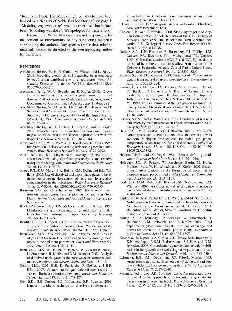
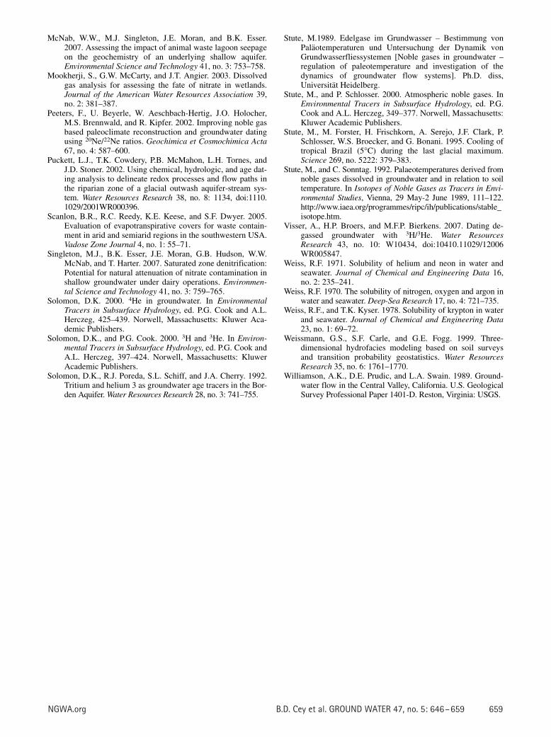
The measured subsurface temperature data allowa direct comparison of modeled NGT to WTT. Groundwater flows along complex and shifting paths because ofintense but ephemeral pumping from relatively shallowirrigation wells in and around the study site. Therefore, itis particularly difficult to identify the recharge area foranything but the shallowest ground water. Furthermore,even if the recharge area of a deeper well were clearlyidentifiable, degassing could affect the calculation ofNGT. For these reasons, samples from the shallowestwell at each field location (wells 2S1, 3S1, 4S1, and 5S1)were considered separately.

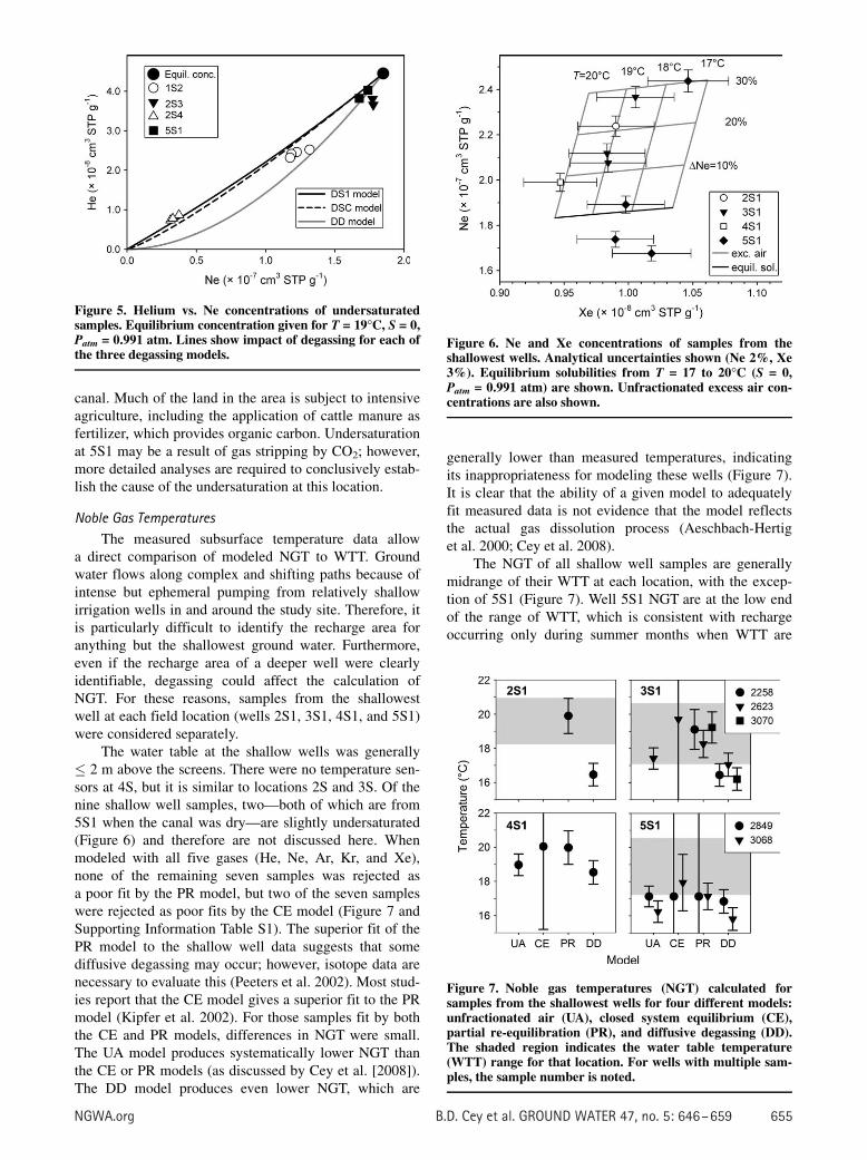
The water table at the shallow wells was generally� 2 m above the screens. There were no temperature sen-sors at 4S, but it is similar to locations 2S and 3S. Of thenine shallow well samples, two—both of which are from5S1 when the canal was dry—are slightly undersaturated(Figure 6) and therefore are not discussed here. Whenmodeled with all five gases (He, Ne, Ar, Kr, and Xe),none of the remaining seven samples was rejected asa poor fit by the PR model, but two of the seven sampleswere rejected as poor fits by the CE model (Figure 7 andSupporting Information Table S1). The superior fit of thePR model to the shallow well data suggests that somediffusive degassing may occur; however, isotope data arenecessary to evaluate this (Peeters et al. 2002). Most stud-ies report that the CE model gives a superior fit to the PRmodel (Kipfer et al. 2002). For those samples fit by boththe CE and PR models, differences in NGT were small.The UA model produces systematically lower NGT thanthe CE or PR models (as discussed by Cey et al. [2008]).The DD model produces even lower NGT, which are

generally lower than measured temperatures, indicatingits inappropriateness for modeling these wells (Figure 7).It is clear that the ability of a given model to adequatelyfit measured data is not evidence that the model reflectsthe actual gas dissolution process (Aeschbach-Hertiget al. 2000; Cey et al. 2008).

The NGT of all shallow well samples are generallymidrange of their WTT at each location, with the excep-tion of 5S1 (Figure 7). Well 5S1 NGT are at the low endof the range of WTT, which is consistent with rechargeoccurring only during summer months when WTT are

Figure 5. Helium vs. Ne concentrations of undersaturatedsamples. Equilibrium concentration given for T = 19�C, S = 0,Patm = 0.991 atm. Lines show impact of degassing for each ofthe three degassing models.

Figure 6. Ne and Xe concentrations of samples from theshallowest wells. Analytical uncertainties shown (Ne 2%, Xe3%). Equilibrium solubilities from T = 17 to 20�C (S = 0,Patm = 0.991 atm) are shown. Unfractionated excess air con-centrations are also shown.

Figure 7. Noble gas temperatures (NGT) calculated forsamples from the shallowest wells for four different models:unfractionated air (UA), closed system equilibrium (CE),partial re-equilibration (PR), and diffusive degassing (DD).The shaded region indicates the water table temperature(WTT) range for that location. For wells with multiple sam-ples, the sample number is noted.

NGWA.org B.D. Cey et al. GROUND WATER 47, no. 5: 646–659 655

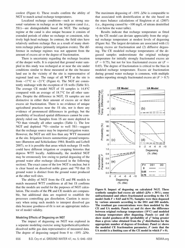
coolest (Figure 4). These results confirm the ability ofNGT to match actual recharge temperatures.

Localized recharge conditions—such as strong sea-sonal variations in recharge as at the irrigation canal (i.e.,5S1)—are distinguishable based on NGT. The rechargeregime at the canal is also unique because it consists ofextended periods of either no recharge or consistent, rela-tively high head recharge. In contrast, the field sites haverelatively uniform recharge flux as a result of many short-term recharge pulses (primarily irrigation events). The dif-ference in recharge regimes was not apparent from theamount of excess air or the degree of fractionation.

There is uncertainty regarding the recharge locationof the deeper wells. It is expected that ground water sam-pled in this study was recharged at or near the site underconditions similar to those measured at the site becauseland use in the vicinity of the site is representative ofregional land use. The range of all WTT at the site isfrom ~17�C to ~21�C (Figure 4). The NGT are consis-tently midrange with the exception of 1S wells (Table S1).The average CE model NGT of 1S samples is 14.8�Ccompared with an average of 18.7�C for all other sam-ples. Despite the difference in NGT, 1S samples are notdistinctive in either their amount of excess air or theirexcess air fractionation. There is no evidence of uniqueagricultural practices near the 1S site, nor is there anyevidence of pronounced differences in geology, but thepossibility of localized spatial differences cannot be com-pletely ruled out. Samples from 1S are more depleted in18O than virtually all other samples (Table 1). The lowNGT and depleted 18O—similar to well 5S1—suggestthat the recharge source may be imported irrigation water.However, the NGT are still less than any WTT measuredat the site. Irrigation lowers summertime ground tempera-ture (Barnston and Schickedanz 1984; Bonfils and Lobell2007), so it is possible that areas which recharge 1S wellscould have different irrigation or cropping histories thatdepress WTT locally. Additionally, the modeled NGTmay be erroneously low owing to partial degassing of theground water after recharge (discussed in the followingsection). The exact cause of the low NGT is unclear, but itis clear based on dissolved noble gases and 18O that 1Sground water is distinct from the ground water producedat the other well sites.

The ability of NGT from the CE and PR models tomatch measured WTT conditions at all but 1S confirmsthat the models are useful for the purposes of NGT calcu-lation. The results of the PR and CE models are compara-ble, but additional data are required to establish theprocesses controlling gas dissolution. Caution is neces-sary when using such models to interpret dissolved gasdata because goodness-of-fit is not an appropriate indica-tor of model validity.

Modeling Effects of Degassing on NGTThe impact of degassing on NGT was explored in

a separate modeling exercise using hypothetical/syntheticdissolved noble gas data representative of measured data.The degree of degassing ranged from 0 to –10% �Ne.

The maximum degassing of –10% �Ne is comparable tothat associated with denitrification at the site based onthe mass balance calculations of Singleton et al. (2007)(i.e., degassing caused by ~100 mg/L of nitrate denitrified~6 m below the water table).

Results indicate that recharge temperature as fittedby the CE model can deviate appreciably from the origi-nal recharge temperature at modest levels of degassing(Figure 8a). The largest deviations are associated with (1)strong excess air fractionation and (2) diffusive degass-ing. The CE modeled recharge temperatures of the de-gassed samples underestimate the original rechargetemperature for initially strongly fractionated excess air(F ¼ 0.75), but not for less fractionated excess air (F ¼0.65). The degree of fractionation is critical to the bias inmodeled recharge temperature. Excess air fractionationduring ground water recharge is common, with multiplestudies reporting strongly fractionated excess air (F . 0.7)

Figure 8. Impact of degassing on calculated NGT. Thesesynthetic samples had excess air added (DNe = 30%), someunfractionated and others fractionated according to the CEmodel (both F = 0.65 and 0.75). Samples were then degassedby various amounts according to the DS1 and DD models.The resultant gas concentrations were then modeled by theCE and UA models. Panels (a) and (b) show the differencebetween original recharge temperature (19�C) and modeledrecharge temperature after degassing. Panels (c) and (d)show model goodness-of-fit (probability of v2 being greaterthan a given value obtained from the v2 distribution for theappropriate number of degrees of freedom). Panel (e) showsthe modeled CE fractionation parameter, F (note that theUA model is a limiting case of the CE model in which F = 0).

656 B.D. Cey et al. GROUND WATER 47, no. 5: 646–659 NGWA.org

(Aeschbach-Hertig et al. 2000, 2002b; Hall et al. 2005).The errors in interpreted recharge temperature are slightlygreater when degassing is controlled by diffusion ratherthan solubility. The prevalence of diffusive degassing isuncertain, because most studies indicate that gas solubil-ity rather than diffusion controls both dissolution (Kipferet al. 2002) and degassing (Visser et al. 2007). However,there is some evidence for diffusive degassing at this sitebased on elemental ratios (1S2, Figure 5).

As shown in this study and in previous work (Blicher-Mathiesen et al. 1998; Dunkle et al. 1993; Fortuin andWillemsen 2005; Klump et al. 2006; Mookherji et al.2003; Puckett et al. 2002; Visser et al. 2007), ground waterdegassing can occur in a variety of settings. Minor degass-ing in the saturated zone after ground water recharge mayhelp explain the NGT biases reported by Castro et al.(2007) and Hall et al. (2005).

Application of an incorrect interpretive model canresult in substantial error in the modeled recharge tempera-ture, especially for samples with strongly fractionatedexcess air (Figure 8b). The UA model systematically cal-culates lower recharge temperatures than the CE model(Aeschbach-Hertig et al. 2000; Cey et al. 2008); therefore,modeling samples with fractionated excess air using theUA model results in underestimation of recharge tempera-ture. This is true regardless of the amount of degassing,including the case of no degassing.

Caution is necessary when applying interpretive mod-els to deduce recharge temperature from dissolved noblegas data. Application of a model that is not representativeof the actual gas dissolution process may yield erroneousresults. The occurrence of degassing after recharge mayalso result in erroneous recharge temperatures. Modelgoodness-of-fit is not necessarily indicative of modelappropriateness (Figure 8c and Figure 8d). Even modelsthat match measured data well may be seriously biased.

ConclusionsThe study examined dissolved noble gases in shallow

ground water at an agricultural site. The local hydrologicregime is heavily impacted by both pumping of groundwater from a shallow unconfined aquifer and importationof surface water for irrigation. Measurements of soil-gaspressure and subsurface temperature defined conditionsunder which recharge occurred.

Samples from multiple wells had dissolved gas con-centrations below equilibrium concentration with respectto atmospheric pressure. The most plausible explanationfor the undersaturated samples is degassing caused by gasstripping. Multiple gas stripping processes occur at thesite (1) within methanogenic liquid manure lagoons,which subsequently recharge, and (2) in the saturatedzone because of denitrification and possibly also CO2

exsolution. The degassing observed has the potential tobias NGT. Hypothetical samples were modeled to explorethe possible effect of degassing on interpreted NGT. Re-sults indicate that relatively minor degassing (,10%�Ne) may cause bias of 2�C. Such errors are problematic

because the degassing may be masked by excess air andthe degassed samples may be fit by a model with a highdegree of certainty. These findings have implications forpaleoclimate research because based on NGT data thetemperature difference since the LGM is 5�C to 7�C(Kipfer et al. 2002). Therefore, caution is necessary whenusing NGT in paleoclimate work.

The role of recharge regime on dissolved noble gaseswas also examined. There are two recharge regimes occur-ring at the study site: (1) focused, higher flux rechargefrom irrigation canal leakage during spring and summeronly (little to no recharge in fall and winter) and (2) lowerflux, spatially and temporally uniform recharge caused byregular flood irrigation. There was no measurable differ-ence in excess air characteristics (amount and degree offractionation) between the two recharge regimes studied.

The study examined the relationship between calcu-lated NGT based on dissolved noble gases and directlymeasured WTT. The complexity of ground water flowand the potential for degassing to affect NGT requiredthat only shallow wells be used to compare NGT toWTT. The NGT from both the CE and PR models reflectthe measured WTT conditions. This finding supports theuse of dissolved noble gases to deduce recharge tempera-tures. Before this study, field-based experimental confir-mation was lacking despite decades of NGT applications.

Although NGT reflect WTT, careful application ofinterpretive models is required because multiple gasdissolution/exsolution processes may contribute to mea-sured dissolved gas concentrations in ground water. A par-ticular model may be fit to measured data, but this does notnecessarily mean that the physical gas dissolution processis accurately represented or that the model results accu-rately represent recharge conditions. Therefore, caution isnecessary when interpreting dissolved noble gas data.

AcknowledgmentsFunding was provided by the California State Water

Resources Control Board Groundwater Ambient Moni-toring and Assessment (GAMA) Program, LawrenceLivermore National Laboratory, the Jackson School ofGeosciences, and the Glenn T. Seaborg Institute (fellow-ship to B.D.C.). We acknowledge Dr. Brad Esser for hissustained support of the project, Dr. Mike Singleton forassistance with sampling and analyses, Mr. WayneCulham for assistance with sample analyses, and thelandowner for access to the study site. This paperbenefited from the insightful and constructive commentsof Drs. Kip Solomon and Stephen van der Hoven, andtwo anonymous reviewers.

Supporting InformationAdditional Supporting Information may be found in

the online version of this article:Table S1. Results of Noble Gas Monitoring.[Corrections added after online publication March 26,

2009: on page 1, the table was incorrectly labeled as a

NGWA.org B.D. Cey et al. GROUND WATER 47, no. 5: 646–659 657

‘‘Results of Noble Bas Monitoring’’, but should have beenlabeled as a ‘‘Results of Noble Gas Monitoring’’; on page 1,‘‘Modeling &q1;was done’’ was incorrect and should havebeen ‘‘Modeling was done’’. We apologize for these errors.]

Please note: Wiley-Blackwell are not responsible forthe content or functionality of any supporting materialssupplied by the authors. Any queries (other than missingmaterial) should be directed to the corresponding authorfor the article.

ReferencesAeschbach-Hertig, W., H. El-Gamal, M. Wieser, and L. Palcsu.

2008. Modeling excess air and degassing in groundwaterby equilibrium partitioning with a gas phase. Water Re-sources Research 44, no. 8: W08449, doi:08410.01029/02007WR006454.

Aeschbach-Hertig, W., U. Beyerle, and R. Kipfer. 2002a. Excessair in groundwater as a proxy for paleo-humidity. In 12th

Annual V. M. Goldschmidt Conference, Davos, Switzerland.Geochimica et Cosmochimica Acta 66, Supp. 1 [abstracts].

Aeschbach-Hertig, W., M. Stute, J.F. Clark, R.F. Reuter, and P.Schlosser. 2002b. A paleotemperature record derived fromdissolved noble gases in groundwater of the Aquia Aquifer(Maryland, USA). Geochimica et Cosmochimica Acta 66,no. 5: 797–817.

Aeschbach-Hertig, W., F. Peeters, U. Beyerle, and R. Kipfer.2000. Palaeotemperature reconstruction from noble gasesin ground water taking into account equilibration with en-trapped air. Nature 405, no. 6790: 1040–1044.

Aeschbach-Hertig, W., F. Peeters, U. Beyerle, and R. Kipfer. 1999.Interpretation of dissolved atmospheric noble gases in naturalwaters.Water Resources Research 35, no. 9: 2779–2792.

Amos, R.T., and K.U. Mayer. 2006. Investigating ebullition ina sand column using dissolved gas analysis and reactivetransport modeling. Environmental Science and Technology40, no. 17: 5361–5367.

Amos, R.T., K.U. Mayer, B.A. Bekins, G.N. Delin, and R.L. Wil-liams. 2005. Use of dissolved and vapor-phase gases to inves-tigate methanogenic degradation of petroleum hydrocarboncontamination in the subsurface. Water Resources Research41, no. 2: W02001, doi:02010.01029/02004WR003433.

Barnston, A.G., and P.T. Schickedanz. 1984. The effect of irriga-tion on warm season precipitation in the southern GreatPlains. Journal of Climate and Applied Meteorology 23, no.6: 865–888.

Blicher-Mathiesen, G., G.W. McCarty, and L.P. Nielsen. 1998.Denitrification and degassing in groundwater estimatedfrom dissolved dinitrogen and argon. Journal of Hydrology208, no. 1–2: 16–24.

Bonfils, C., and D. Lobell. 2007. Empirical evidence for a recentslowdown in irrigation-induced cooling. Proceedings of theNational Academy of Sciences 104, no. 34: 13582–13587.

Brennwald, M.S., R. Kipfer, and D.M. Imboden. 2005. Releaseof gas bubbles from lake sediment traced by noble gas iso-topes in the sediment pore water. Earth and Planetary Sci-ence Letters 235, no. 1–2: 31–44.

Brennwald, M.S., M. Hofer, F. Peeters, W. Aeschbach-Hertig,K. Strassmann, R. Kipfer, and D.M. Imboden. 2003. Analysisof dissolved noble gases in the pore water of lacustrine sedi-ments. Limnology and Oceanography: Methods 1, 51–62.

Castro, M.C., C.M. Hall, D. Patriarche, P. Goblet, and B.R.Ellis. 2007. A new noble gas paleoclimate record inTexas—Basic assumptions revisited. Earth and PlanetaryScience Letters 257, no. 1–2: 170–187.

Cey, B.D., G.B. Hudson, J.E. Moran, and B.R. Scanlon. 2008.Impact of artificial recharge on dissolved noble gases in

groundwater in California. Environmental Science andTechnology 42, no. 4: 1017–1023.

Clever, H.L., ed. 1979. Krypton, Xenon and Radon. Elmsford,New York: Pergamon Press.

Coplen, T.B., and C. Kendall. 2000. Stable hydrogen and oxy-gen isotope ratios for selected sites of the U.S. GeologicalSurvey’s NASQAN and benchmark surface-water net-works. U.S. Geological Survey Open-File Report 00-160.Reston, Virginia: USGS.

Dunkle, S.A., L.N. Plummer, E. Busenberg, P.J. Phillips, J.M.Denver, P.A. Hamilton, R.L. Michel, and T.B. Coplen.1993. Chlorofluorocarbons (CCl3F and CCl2F2) as datingtools and hydrologic tracers in shallow groundwater of theDelmarva Peninsula, Atlantic Coastal Plain, United States.Water Resources Research 29, no. 12: 3837–3860.

Epstein, S., and T.K. Mayeda. 1953. Variation of 18O content ofwaters from natural sources. Geochimica et CosmochimicaActa 4, no. 5: 213–224.

Farrera, I., S.P. Harrison, I.C. Prentice, G. Ramstein, J. Guiot,P.J. Bartlein, R. Bonnefille, M. Bush, W. Cramer, U. vonGrafenstein, K. Holmgren, H. Hooghiemstra, G. Hope, D.Jolly, S.-E. Lauritzen, Y. Ono, S. Pinot, M. Stute, and G.Yu. 1999. Tropical climates at the last glacial maximum: Anew synthesis of terrestrial paleoclimate data. I. Vegetation,lake-levels and geochemistry. Climate Dynamics 15, no.11: 823–856.

Fortuin, N.P.M., and A. Willemsen. 2005. Exsolution of nitrogenand argon by methanogenesis in Dutch ground water. Jour-nal of Hydrology 301, no. 1–4: 1–13.

Hall, C.M., M.C. Castro, K.C. Lohmann, and L. Ma. 2005.Noble gases and stable isotopes in a shallow aquifer insouthern Michigan: Implications for noble gas paleo-temperature reconstructions for cool climates. GeophysicalResearch Letters 32, no. 18: L18404, doi:18410.11029/12005GL023582.

Heaton, T.H.E., and J.C. Vogel. 1981. ‘‘Excess air’’ in ground-water. Journal of Hydrology 50, no. 1–3: 201–216.

Holocher, J.O., F. Peeters, W. Aeschbach-Hertig, M. Hofer,M. Brennwald, W. Kinzelbach, and R. Kipfer. 2002. Exper-imental investigations on the formation of excess air inquasi-saturated porous media. Geochimica et Cosmochi-mica Acta 66, no. 23: 4103–4117.

Istok, J.D., M.M. Park, A.D. Peacock, M. Oostrom, and T.M.Wietsma. 2007. An experimental investigation of nitrogengas produced during denitrification. Ground Water 45, no.4: 461–467.

Kipfer, R., W. Aeschbach-Hertig, F. Peeters, and M. Stute. 2002.Noble gases in lakes and ground waters. In Noble Gases inGeochemistry and Cosmochemistry, ed. D. Porcelli, C. J.Ballentine, and R. Wieler, 615–700. Washington, DC: Min-eralogical Society of America.

Klump, S., Y. Tomonaga, P. Kienzler, W. Kinzelbach, T.Baumann, D.M. Imboden, and R. Kipfer. 2007. Fieldexperiments yield new insights into gas exchange andexcess air formation in natural porous media. Geochimicaet Cosmochimica Acta 71, no. 6: 1385–1397.

Klump, S., R. Kipfer, O.A. Cirpka, C.F. Harvey, M.S. Brennwald,K.N. Ashfaque, A.B.M. Badruzzaman, S.J. Hug, and D.M.Imboden. 2006. Groundwater dynamics and arsenic mobili-zation in Bangladesh assessed using noble gases and tritium.Environmental Science and Technology 40, no. 1: 243–250.

Lehmann, B.E., S.N. Davis, and J.T. Fabryka-Martin. 1993.Atmospheric and subsurface sources of stable and radioac-tive nuclides used for groundwater dating. Water ResourcesResearch 29, no. 7: 2027–2040.

Manning, A.H., and D.K. Solomon. 2005. An integrated envi-ronmental tracer approach to characterizing groundwatercirculation in a mountain block. Water Resources Research41, no. 12: W12412, doi:12410.11029/12005WR004178.

658 B.D. Cey et al. GROUND WATER 47, no. 5: 646–659 NGWA.org

McNab, W.W., M.J. Singleton, J.E. Moran, and B.K. Esser.2007. Assessing the impact of animal waste lagoon seepageon the geochemistry of an underlying shallow aquifer.Environmental Science and Technology 41, no. 3: 753–758.

Mookherji, S., G.W. McCarty, and J.T. Angier. 2003. Dissolvedgas analysis for assessing the fate of nitrate in wetlands.Journal of the American Water Resources Association 39,no. 2: 381–387.

Peeters, F., U. Beyerle, W. Aeschbach-Hertig, J.O. Holocher,M.S. Brennwald, and R. Kipfer. 2002. Improving noble gasbased paleoclimate reconstruction and groundwater datingusing 20Ne/22Ne ratios. Geochimica et Cosmochimica Acta67, no. 4: 587–600.

Puckett, L.J., T.K. Cowdery, P.B. McMahon, L.H. Tornes, andJ.D. Stoner. 2002. Using chemical, hydrologic, and age dat-ing analysis to delineate redox processes and flow paths inthe riparian zone of a glacial outwash aquifer-stream sys-tem. Water Resources Research 38, no. 8: 1134, doi:1110.1029/2001WR000396.

Scanlon, B.R., R.C. Reedy, K.E. Keese, and S.F. Dwyer. 2005.Evaluation of evapotranspirative covers for waste contain-ment in arid and semiarid regions in the southwestern USA.Vadose Zone Journal 4, no. 1: 55–71.

Singleton, M.J., B.K. Esser, J.E. Moran, G.B. Hudson, W.W.McNab, and T. Harter. 2007. Saturated zone denitrification:Potential for natural attenuation of nitrate contamination inshallow groundwater under dairy operations. Environmen-tal Science and Technology 41, no. 3: 759–765.

Solomon, D.K. 2000. 4He in groundwater. In EnvironmentalTracers in Subsurface Hydrology, ed. P.G. Cook and A.L.Herczeg, 425–439. Norwell, Massachusetts: Kluwer Aca-demic Publishers.

Solomon, D.K., and P.G. Cook. 2000. 3H and 3He. In Environ-mental Tracers in Subsurface Hydrology, ed. P.G. Cook andA.L. Herczeg, 397–424. Norwell, Massachusetts: KluwerAcademic Publishers.

Solomon, D.K., R.J. Poreda, S.L. Schiff, and J.A. Cherry. 1992.Tritium and helium 3 as groundwater age tracers in the Bor-den Aquifer.Water Resources Research 28, no. 3: 741–755.

Stute, M.1989. Edelgase im Grundwasser – Bestimmung vonPalaotemperaturen und Untersuchung der Dynamik vonGrundwasserfliessystemen [Noble gases in groundwater –regulation of paleotemperature and investigation of thedynamics of groundwater flow systems]. Ph.D. diss,Universitat Heidelberg.

Stute, M., and P. Schlosser. 2000. Atmospheric noble gases. InEnvironmental Tracers in Subsurface Hydrology, ed. P.G.Cook and A.L. Herczeg, 349–377. Norwell, Massachusetts:Kluwer Academic Publishers.

Stute, M., M. Forster, H. Frischkorn, A. Serejo, J.F. Clark, P.Schlosser, W.S. Broecker, and G. Bonani. 1995. Cooling oftropical Brazil (5�C) during the last glacial maximum.Science 269, no. 5222: 379–383.

Stute, M., and C. Sonntag. 1992. Palaeotemperatures derived fromnoble gases dissolved in groundwater and in relation to soiltemperature. In Isotopes of Noble Gases as Tracers in Envi-ronmental Studies, Vienna, 29 May-2 June 1989, 111–122.http://www.iaea.org/programmes/ripc/ih/publications/stable_isotope.htm.

Visser, A., H.P. Broers, and M.F.P. Bierkens. 2007. Dating de-gassed groundwater with 3H/3He. Water ResourcesResearch 43, no. 10: W10434, doi:10410.11029/12006WR005847.

Weiss, R.F. 1971. Solubility of helium and neon in water andseawater. Journal of Chemical and Engineering Data 16,no. 2: 235–241.

Weiss, R.F. 1970. The solubility of nitrogen, oxygen and argon inwater and seawater. Deep-Sea Research 17, no. 4: 721–735.

Weiss, R.F., and T.K. Kyser. 1978. Solubility of krypton in waterand seawater. Journal of Chemical and Engineering Data23, no. 1: 69–72.

Weissmann, G.S., S.F. Carle, and G.E. Fogg. 1999. Three-dimensional hydrofacies modeling based on soil surveysand transition probability geostatistics. Water ResourcesResearch 35, no. 6: 1761–1770.

Williamson, A.K., D.E. Prudic, and L.A. Swain. 1989. Ground-water flow in the Central Valley, California. U.S. GeologicalSurvey Professional Paper 1401-D. Reston, Virginia: USGS.

NGWA.org B.D. Cey et al. GROUND WATER 47, no. 5: 646–659 659

Supporting Information for: Cey et al. 2009, Evaluation of Noble Gas Recharge Temperatures in a Shallow Unconfined Aquifer

Table S1. Results of noble gas modeling. Modeling was done using He, Ne, Ar, Kr, and Xe for the UA, PR, and CE models. Additional modeling was done using only Ne, Ar, Kr, and Xe with the CE model. Results rejected because of poor fitting (i.e. p < 0.05) are not shown. Samples with large recharge temperature uncertainties are included despite the obvious non-uniqueness of the result.

UA PR CE CE (excluding He)

Well Sample p T

(°C) +/-

(°C) Ne (%)

p T

(°C) +/-

(°C) Ne (%)

R p T

(°C) +/-

(°C) Ne (%)

F p T

(°C) +/-

(°C) Ne (%)

F

1S2 2250A 0.00 - - - 0.00 - - - - 0.00 - - - - 0.00 - - - - 2250B 0.00 - - - 0.00 - - - - 0.00 - - - - 0.00 - - - - 2634 0.00 - - - 0.00 - - - - 0.00 - - - - 0.00 - - - - 3065 0.00 - - - 0.00 - - - - 0.00 - - - - 0.00 - - - -

1S3 1864A 0.06 13.1 0.6 26 0.10 13.7 0.7 30 0.24 0.77 16.3 2.5 31 0.71 0.56 16.3 2.4 31 0.70 1864B 0.02 - - - 0.03 - - - - 0.76 17.8 5.6 29 0.75 0.90 19.5 22.8 32 0.74 1862A 0.65 13.7 0.6 54 0.44 13.7 0.7 54 0.00 0.62 14.6 1.2 56 0.27 0.71 15.0 1.4 55 0.38 1862B 0.99 13.4 0.7 66 1.00 13.5 0.8 67 0.03 0.98 13.6 1.1 67 0.09 0.95 13.5 1.2 67 0.04 1871A 0.31 13.0 0.6 14 0.40 13.4 0.7 17 0.31 0.62 14.6 2.0 16 0.82 0.43 14.6 1.8 17 0.80 1871B 0.33 14.4 0.7 70 0.09 14.2 0.8 67 0.00 0.15 14.3 1.1 69 0.00 0.93 14.9 1.3 66 0.24 1874A 0.14 12.6 0.6 16 0.08 12.8 0.7 18 0.15 0.85 16.5 7.5 21 0.81 0.57 16.4 11.9 21 0.81 1874B 0.23 12.8 0.6 13 0.58 13.4 0.7 17 0.44 0.58 14.7 2.4 16 0.83 0.94 14.7 2.0 17 0.80 1880A 0.02 - - - 0.08 13.0 0.7 15 0.65 0.18 14.7 6.2 14 0.87 0.38 16.1 20.0 18 0.84 1880B 0.01 - - - 0.07 13.1 0.7 18 0.59 0.17 14.9 5.1 16 0.84 0.40 16.3 13.3 20 0.82 1883 0.00 - - - 0.00 - - - - 0.00 - - - - 0.00 - - - - 2253 0.08 12.3 0.6 8 0.31 13.0 0.7 13 0.78 0.23 14.1 5.4 11 0.89 0.58 15.7 14.9 15 0.87 2632 0.02 - - - 0.17 12.9 0.8 11 1.20 0.07 13.4 5.6 8 0.92 0.31 14.8 17.5 13 0.88

1S4 1863A 0.13 12.4 0.6 18 0.23 13.0 0.7 22 0.31 0.80 15.2 2.9 22 0.78 0.93 15.3 2.6 23 0.77 1863B 0.42 14.0 0.6 53 0.80 14.6 0.8 57 0.13 0.80 15.4 1.3 56 0.36 0.83 15.2 1.3 57 0.29 1866A 0.54 13.9 0.6 49 0.21 13.7 0.7 47 0.00 0.29 13.8 1.0 48 0.00 0.68 14.2 1.3 46 0.30 1866B 0.69 13.7 0.6 49 0.34 13.6 0.7 47 0.00 0.42 13.7 1.0 48 0.00 0.93 14.0 1.2 46 0.28 1869A 0.49 13.3 0.6 38 0.24 13.2 0.7 37 0.00 0.23 13.3 1.0 37 0.00 0.19 13.2 1.2 36 0.00 1869B 0.83 14.9 0.6 39 0.73 15.1 0.7 40 0.05 0.94 15.7 1.3 41 0.39 0.77 15.8 1.4 41 0.42 1873A 0.55 14.1 0.6 38 0.27 14.0 0.7 37 0.00 0.33 14.1 1.0 37 0.00 0.42 14.6 1.3 36 0.45 1873B 0.86 14.2 0.6 38 0.60 14.1 0.7 37 0.00 0.66 14.1 1.0 37 0.00 0.70 14.4 1.2 36 0.32 1884 0.08 15.4 0.6 34 0.02 - - - - 0.03 - - - - 0.55 17.0 1.8 31 0.67 2252 0.64 14.9 0.6 33 0.28 14.6 0.7 31 0.00 0.34 14.9 1.0 32 0.00 0.75 15.0 1.2 30 0.37 2631 0.43 14.6 0.6 31 0.24 14.6 0.7 30 0.00 0.35 15.7 1.3 33 0.54 0.62 16.4 1.7 31 0.66

1S5 1865 0.01 - - - 0.48 14.0 0.7 25 0.56 0.13 15.3 2.4 22 0.78 0.99 15.3 1.8 25 0.72 1870A 0.00 - - - 0.00 - - - - 0.00 - - - - 0.24 13.3 1.1 11 0.00 1870B 0.00 - - - 0.00 - - - - 0.00 - - - - 0.00 - - - - 1868 0.00 - - - 0.00 - - - - 0.00 - - - - 0.00 - - - - 2251 0.00 - - - 0.00 - - - - 0.00 - - - - 0.14 15.5 ∞ 0 0.00

2S1 3352 0.00 - - - 0.59 20.2 1.1 22 1.33 0.00 - - - - 0.49 18.8 1.3 21 0.00

2S2 2123 0.00 - - - 0.12 23.5 0.9 32 0.47 0.00 - - - - 0.05 - - - - 2259A 0.05 - - - 0.34 22.6 0.9 24 0.47 0.02 - - - - 0.15 21.7 1.4 23 0.00 2259B 0.01 - - - 0.37 23.4 0.9 26 0.60 0.01 - - - - 0.17 22.3 1.4 23 0.00 2627 0.00 - - - 0.25 22.8 0.9 23 0.69 0.00 - - - - 0.13 21.7 1.3 22 0.00

2S3 2124 0.00 - - - 0.00 - - - - 0.00 - - - - 0.20 21.7 ∞ 0 0.00 2628A 0.00 - - - 0.00 - - - - 0.00 - - - - 0.20 22.7 ∞ 0 0.00 2628B 0.00 - - - 0.00 - - - - 0.00 - - - - 0.00 - - - -

2S4 2125 0.00 - - - 0.00 - - - - 0.00 - - - - 0.00 - - - - 2261 0.00 - - - 0.00 - - - - 0.00 - - - - 0.00 - - - - 2633A 0.00 - - - 0.00 - - - - 0.00 - - - - 0.00 - - - - 2633B 0.00 - - - 0.00 - - - - 0.00 - - - - 0.00 - - - -

3S1 2258 0.01 - - - 0.73 19.4 1.2 13 1.79 0.01 - - - - 0.57 21.9 7.1 15 0.86 2623 0.06 17.4 0.6 11 0.26 18.2 0.8 15 0.68 0.23 19.7 5.7 13 0.87 0.56 21.6 17.3 17 0.84 3070 0.00 - - - 0.78 19.3 0.9 28 0.89 0.00 - - - - 0.52 18.4 1.3 28 0.26

3S2 2257 0.00 - - - 0.00 - - - - 0.00 - - - - 0.02 - - - - 3071 0.00 - - - 0.30 26.8 2.5 31 2.45 0.00 - - - - 0.14 21.9 1.5 28 0.52

3S3 2256 0.08 16.0 0.6 11 0.33 16.8 0.8 16 0.62 0.25 18.3 4.8 14 0.86 0.53 21.0 7.4 19 0.84

3S4 2255 0.00 - - - 0.00 - - - - 0.00 - - - - 0.10 19.0 ∞ 0 0.00

4S1 2670 0.20 18.9 0.6 5 0.70 19.9 1.0 9 1.28 0.21 20.0 4.8 6 0.93 0.61 21.8 10.5 10 0.90

4S2 2264 0.01 - - - 0.62 17.4 0.8 53 0.33 0.05 - - - - 0.34 17.7 1.4 53 0.33 2625 0.17 16.4 0.7 47 0.86 17.2 0.8 53 0.21 0.43 18.1 1.5 50 0.44 0.88 17.7 1.4 53 0.31

4S3 2262A 0.53 16.9 0.7 35 0.64 17.3 0.8 38 0.13 0.82 18.3 1.5 38 0.51 0.58 18.2 1.5 38 0.48 2262B 0.45 17.3 0.7 44 0.42 17.7 0.8 46 0.10 0.53 18.5 1.4 46 0.40 0.27 18.5 1.4 46 0.38 2636A 0.30 17.9 0.7 35 0.84 18.7 0.8 40 0.22 0.53 19.5 1.5 38 0.52 0.71 19.1 1.4 40 0.40 2636B 0.08 18.0 0.7 40 0.89 19.0 0.8 46 0.27 0.20 19.8 1.6 43 0.50 0.68 19.3 1.4 46 0.32

4S4 2263A 0.00 - - - 0.17 27.1 4.0 35 3.15 0.00 - - - - 0.57 21.9 4.8 31 0.73 2263B 0.73 17.9 0.6 15 0.47 17.8 0.7 14 0.00 0.47 17.8 1.1 14 0.00 0.59 17.7 1.2 12 0.00

5S1 2254 0.00 - - - 0.00 - - - - 0.00 - - - - 0.00 - - - - 2626 0.00 - - - 0.00 - - - - 0.00 - - - - 0.00 - - - - 2849 0.39 17.2 0.6 0 0.22 17.2 ∞ 0 0.00 0.22 17.2 ∞ 0 0.00 0.30 17.9 21.1 2 0.98 3068 0.12 16.3 0.6 25 0.85 17.2 0.8 30 0.35 0.25 17.9 1.6 28 0.66 0.65 17.5 1.4 30 0.52

I1 1889 0.03 - - - 0.31 17.8 0.9 103 0.17 0.49 19.7 1.7 101 0.27 0.54 19.3 1.6 103 0.23

I2 1890 0.20 18.8 0.7 60 0.09 18.7 0.8 59 0.00 0.12 19.7 1.4 62 0.23 0.14 20.4 1.6 60 0.39

I3 1771 0.00 - - - 0.00 - - - - 0.00 - - - - 0.25 12.3 1.1 6 0.00

I4 1888 0.24 17.1 0.8 169 0.32 17.8 1.0 175 0.07 0.85 19.4 1.6 175 0.10 0.57 19.5 1.7 175 0.10

I5 1886 0.87 16.6 0.7 111 0.93 16.9 0.9 114 0.04 0.77 17.0 1.3 112 0.05 0.73 16.8 1.4 113 0.00