Hu et al. Environmental Systems Research (2015) 4:4 DOI 10.1186/s40068-015-0031-4

RESEARCH ARTICLE Open Access

Evaluation of parameter uncertainties in nonlinearregression using Microsoft Excel SpreadsheetWei Hu1, Jing Xie1, Henry Wai Chau2 and Bing Cheng Si1*

Abstract

Background: Nonlinear relationships are common in the environmental discipline. Spreadsheet packages such asMicrosoft Excel come with an add-on for nonlinear regression, but parameter uncertainty estimates are not yetavailable. The purpose of this paper is to use Monte Carlo and bootstrap methods to estimate nonlinear parameteruncertainties with a Microsoft Excel spreadsheet. As an example, uncertainties of two parameters (α and n) for a soilwater retention curve are estimated.

Results: The fitted parameters generally do not follow a normal distribution. Except for the upper limit of α usingthe bootstrap method, the lower and upper limits of α and n obtained by these two methods are slightly greaterthan those obtained using the SigmaPlot software which linearlizes the nonlinear model.

Conclusions: Since the linearization method is based on the assumption of normal distribution of parametervalues, the Monte Carlo and bootstrap methods may be preferred to the linearization method.

Keywords: Bootstrap; Monte Carlo; Soil water retention; Parameter uncertainty; Excel

BackgroundNonlinear relationships are common in natural and envir-onmental sciences (Wraith and Or 1998; Luo et al. 2003;Cwiertny and Roberts 2005). As a result, there are manysoftware packages (such as SAS and MathCAD) that imple-ment nonlinear parameter estimation. However, spread-sheet techniques are easier to learn than other specializedmathematical programs for nonlinear parameter estimation,because no programming skills are needed in spreadsheetsto develop their own parameter estimation routines (Wraithand Or 1998). In addition, spreadsheets have the merits ofwide accessibility and powerful computation in terms of fit-ting nonlinear models. For these reasons, spreadsheets suchas Microsoft Excel are widely suggested to make nonlinearparameter estimation (Harris 1998; Smith et al. 1998;Wraith and Or 1998; Brown 2001; Berger 2007).Parameter uncertainty refers to lack of knowledge re-

garding the exact true value of a quantity (Tong et al.2012). Different observations are usually obtained whenexperiments are repeated, resulting in different values ofparameters. It is usually expressed as an interval of

* Correspondence: bing.si@usask.ca1Department of Soil Science, University of Saskatchewan, Saskatoon, SK S7N5A8, CanadaFull list of author information is available at the end of the article

© 2015 Hu et al.; licensee Springer. This is an OAttribution License (http://creativecommons.orin any medium, provided the original work is p

parameter values at a certain confidence level, say, 95%. Itis also expressed as the standard error of the mean by as-suming normal distribution of parameter values. Param-eter uncertainty can be used to judge the degree ofreliability of the parameter estimates, which is importantto making decisions for environmental management. Forthese reasons, estimation of parameter uncertainties is sig-nificant for nonlinear parameter estimates. However, rela-tively less work has focused on the nonlinear parameteruncertainty estimates using spreadsheet packages.Parameter uncertainty can be obtained exactly by assum-

ing normal distribution of a parameter in linear regression,but not in nonlinear regression. Nonlinear regression pro-grams usually give the parameter uncertainty by calculatingthe standard error of the mean, and assuming linear rela-tionship between variables in the vicinity of the estimatedparameter values and normal distribution of parametervalues. Furthermore, this method usually involves evaluat-ing a Hessian matrix (a square matrix of second-order par-tial derivatives of a scalar-valued function to describe thelocal curvature of a function of many variables) or an in-equality, which makes it more complicated and time de-manding (Brown 2001). More general methods such asMonte Carlo and bootstrap simulation can be used to esti-mate the parameter uncertainties. Both methods have their

pen Access article distributed under the terms of the Creative Commonsg/licenses/by/4.0), which permits unrestricted use, distribution, and reproductionroperly credited.

Hu et al. Environmental Systems Research (2015) 4:4 Page 2 of 12

own advantages: while the Monte Carlo method is basedon a theoretical probability distribution of a variable, thebootstrap method has no assumption on the probabilitydistribution of a variable and thus has no limits on sam-pling size. Among numerous related applications are testingfire ignition selectivity of different landscape characteristicsusing the Monte Carlo simulation (Conedera et al. 2011)and estimating uncertainty of greenhouse gas emissionsusing the bootstrap simulation (Tong et al. 2012). However,parameter uncertainties estimation in spreadsheets usingthe Monte Carlo and bootstrap methods has been rarelydiscussed.Both nonlinear parameter values and their associated un-

certainties are important for decision making and thusshould be implemented in spreadsheet program like Excel.Microsoft Excel spreadsheets have other advantages includ-ing their general facility for data input and management,ease in implementing calculations, and often advancedgraphics and reporting capabilities (Wraith and Or 1998).These advantages are likely to make the use of spreadsheetsto quantify parameter uncertainties more desirable.The objective of this paper is to apply the Monte Carlo

and bootstrap simulations to obtain parameter uncer-tainties with a Microsoft Excel spreadsheet. In addition,the influences of number of simulation on uncertaintyestimates are also discussed. For this, we use as an ex-ample, a common soil physical property - soil water

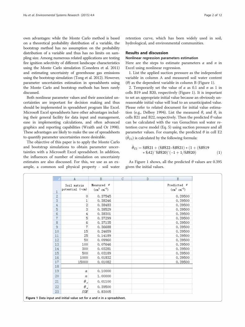
Figure 1 Data input and initial value set for α and n in a spreadsheet

retention curve, which has been widely used in soil,hydrological, and environmental communities.

Results and discussionNonlinear regression parameters estimationHere are the steps to estimate parameters α and n inExcel using nonlinear regression.1. List the applied suction pressure as the independent

variable in column A and measured soil water content(θ) as the dependent variable in column B (Figure 1).2. Temporarily set the value of α as 0.1 and n as 1 in

cells B19 and B20, respectively (Figure 1). It is importantto set an appropriate initial value because an obviously un-reasonable initial value will lead to an unanticipated value.Please refer to related document for initial value estima-tion (e.g., Delboy 1994). List the measured θr and θs incells B21 and B22, respectively. Then the predicted θ valuecan be calculated with the van Genuchten soil water re-tention curve model (Eq. 5) using suction pressure and allparameter values. For example, the predicted θ in cell E2

(θ̂E2) is calculated by the following formula:

θ̂E2 ¼ $B$21þ ð$B$22−$B$21Þ � ð1þ ð$B$19� $A2Þ^$B$20Þ̂ −1þ 1=$B$20ð Þ ð1Þ

As Figure 1 shows, all the predicted θ values are 0.395given the initial values.

.

Hu et al. Environmental Systems Research (2015) 4:4 Page 3 of 12

3. Calculate the sum of squared residuals (SSE) usingExcel function SUMXMY2 in cell B23 by entering“SUMXMY2(B2 : B17, E2 : E17)”. We obtain 0.83005 forSSE for the given initial parameter values (Figure 1).4. The model obtains the maximum likelihood when

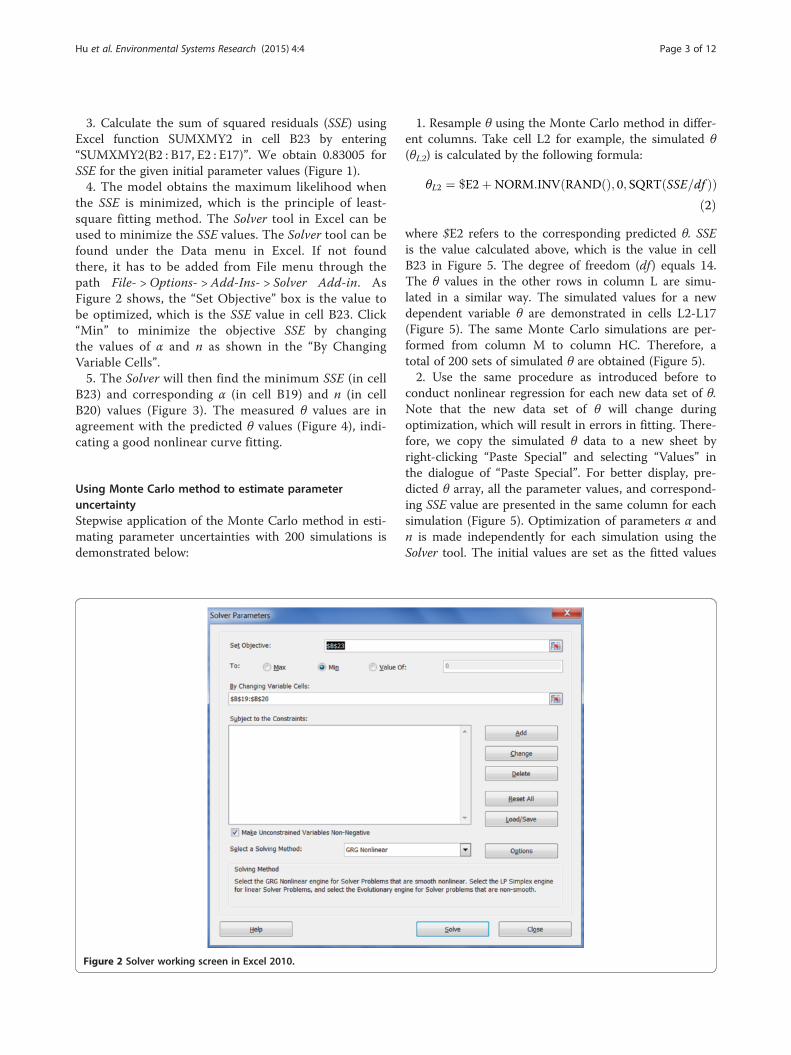
the SSE is minimized, which is the principle of least-square fitting method. The Solver tool in Excel can beused to minimize the SSE values. The Solver tool can befound under the Data menu in Excel. If not foundthere, it has to be added from File menu through thepath File- > Options- > Add-Ins- > Solver Add-in. AsFigure 2 shows, the “Set Objective” box is the value tobe optimized, which is the SSE value in cell B23. Click“Min” to minimize the objective SSE by changingthe values of α and n as shown in the “By ChangingVariable Cells”.5. The Solver will then find the minimum SSE (in cell

B23) and corresponding α (in cell B19) and n (in cellB20) values (Figure 3). The measured θ values are inagreement with the predicted θ values (Figure 4), indi-cating a good nonlinear curve fitting.

Using Monte Carlo method to estimate parameteruncertaintyStepwise application of the Monte Carlo method in esti-mating parameter uncertainties with 200 simulations isdemonstrated below:

Figure 2 Solver working screen in Excel 2010.

1. Resample θ using the Monte Carlo method in differ-ent columns. Take cell L2 for example, the simulated θ(θL2) is calculated by the following formula:

θL2 ¼ $E2þNORM:INV RANDðÞ; 0; SQRT SSE=dfð Þð Þð2Þ

where $E2 refers to the corresponding predicted θ. SSEis the value calculated above, which is the value in cellB23 in Figure 5. The degree of freedom (df ) equals 14.The θ values in the other rows in column L are simu-lated in a similar way. The simulated values for a newdependent variable θ are demonstrated in cells L2-L17(Figure 5). The same Monte Carlo simulations are per-formed from column M to column HC. Therefore, atotal of 200 sets of simulated θ are obtained (Figure 5).2. Use the same procedure as introduced before to

conduct nonlinear regression for each new data set of θ.Note that the new data set of θ will change duringoptimization, which will result in errors in fitting. There-fore, we copy the simulated θ data to a new sheet byright-clicking “Paste Special” and selecting “Values” inthe dialogue of “Paste Special”. For better display, pre-dicted θ array, all the parameter values, and correspond-ing SSE value are presented in the same column for eachsimulation (Figure 5). Optimization of parameters α andn is made independently for each simulation using theSolver tool. The initial values are set as the fitted values

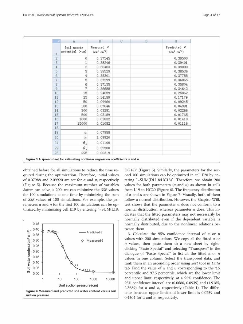
Figure 3 A spreadsheet for estimating nonlinear regression coefficients α and n.

Hu et al. Environmental Systems Research (2015) 4:4 Page 4 of 12

obtained before for all simulations to reduce the time re-quired during the optimization. Therefore, initial valuesof 0.07988 and 2.09920 are set for α and n, respectively(Figure 5). Because the maximum number of variablesSolver can solve is 200, we can minimize the SSE valuesfor 100 simulations at one time by minimizing the sumof SSE values of 100 simulations. For example, the pa-rameters α and n for the first 100 simulations can be op-timized by minimizing cell E19 by entering “=SUM(L18:

Figure 4 Measured and predicted soil water content versus soilsuction pressure.

DG18)” (Figure 5). Similarly, the parameters for the sec-ond 100 simulations can be optimized in cell E20 by en-tering “=SUM(DH18:HC18)”. Therefore, we obtain 200values for both parameters (α and n) as shown in cellsfrom L19 to HC20 (Figure 6). The frequency distributionof α and n are shown in Figure 7. Visually, both of themfollow a normal distribution. However, the Shapiro-Wilktest shows that the parameter α does not conform to anormal distribution, whereas parameter n does. This in-dicates that the fitted parameters may not necessarily benormally distributed even if the dependent variable isnormally distributed, due to the nonlinear relations be-tween them.3. Calculate the 95% confidence interval of α or n

values with 200 simulations. We copy all the fitted α orn values, then paste them to a new sheet by right-clicking “Paste Special” and selecting “Transpose” in thedialogue of “Paste Special” to list all the fitted α or nvalues in one column. Select the transposed data, andrank them in an ascending order using Sort tool in Datatab. Find the value of α and n corresponding to the 2.5percentile and 97.5 percentile, which are the lower limitand upper limit, respectively, at a 95% confidence. The95% confidence interval are (0.0680, 0.0939) and (1.9185,2.3689) for α and n, respectively (Table 1). The differ-ence between upper limit and lower limit is 0.0259 and0.4504 for α and n, respectively.

Figure 5 Resampling dependent variable θ using Monte Carlo method and initial values set (only the first 5 simulations are shown).

Hu et al. Environmental Systems Research (2015) 4:4 Page 5 of 12

Using bootstrap method to estimate parameteruncertaintyStepwise application of the bootstrap method in estimat-ing parameter uncertainties with 200 simulations isdemonstrated as follows:1. Resample θ using the bootstrap method in different

columns (Figure 8). Take cell L2 for example, thesimulated θ (θL2) can be calculated by the followingformula:

θL2 ¼ $E2þ INDEXð$C : $C; INTðRANDðÞ � 16þ 2ÞÞð3Þ

where the function INDEX is used to randomly select aresidue value from row 2 to row 17 in column C (the re-sidual is calculated by subtracting predicted θ from theoriginal θ). The θ values at other rows in column L andin other columns (column M to column HC) are simu-lated in a similar way. Here, 2 in the right hand side ofEq. (3) means that data start at second row.

2. Similar to the Monte Carlo method, parameters αand n for all simulations are fitted by minimizing thesum of every 100 SSE values using the Solver tool(Figures 8 and 9). Therefore, we can also obtain 200values for both parameters (α and n) as shown in cellsfrom L19 to HC20 (Figure 9). The frequency distributionof α and n are shown in Figure 10. They also visually fol-low a normal distribution. However, the Shapiro-Wilktest shows that the parameter α does not conform tonormal distribution, whereas parameter n does.3. Similar to the Monte Carlo method, the 95% confi-

dence intervals for these two parameters are calculated.They are (0.0680, 0.0925) and (1.9172, 2.3356), for α andn respectively (Table 1). The corresponding differencebetween upper limit and lower limit is 0.0245 and0.4183 for α and n, respectively.

Influences of number of simulation on parameteruncertainty analysisDatasets of fitted values with different numbers of simula-tions are obtained using a similar method as demonstrated

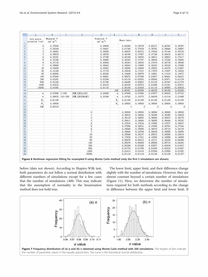
Figure 6 Nonlinear regression fitting for resampled θ using Monte Carlo method (only the first 5 simulations are shown).

Hu et al. Environmental Systems Research (2015) 4:4 Page 6 of 12

before (data not shown). According to Shapiro-Wilk test,both parameters do not follow a normal distribution withdifferent numbers of simulations except for a few casesthat the number of simulations ≤400. This may indicatethat the assumption of normality in the linearizationmethod does not hold true.

Figure 7 Frequency distribution of (a) α and (b) n obtained using Mothe number of parameter values in the equally spaced bins. The curve is th

The lower limit, upper limit, and their difference changeslightly with the number of simulations. However, they arealmost constant beyond a certain number of simulations(Figure 11). Here, we determine the number of simula-tions required for both methods according to the changein difference between the upper limit and lower limit. If

nte Carlo method with 200 simulations. The heights of bars indicatee theoretical normal distribution.

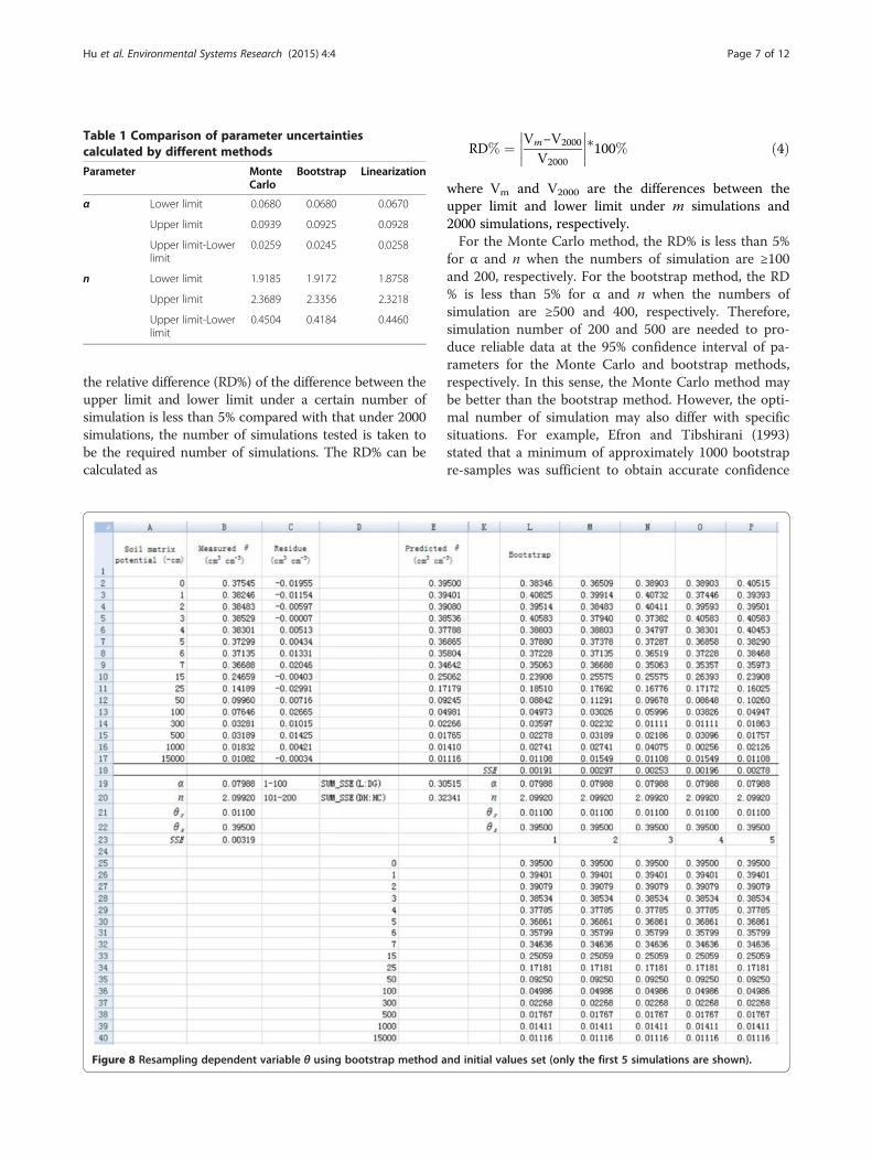
Table 1 Comparison of parameter uncertaintiescalculated by different methods

Parameter MonteCarlo

Bootstrap Linearization

α Lower limit 0.0680 0.0680 0.0670

Upper limit 0.0939 0.0925 0.0928

Upper limit-Lowerlimit

0.0259 0.0245 0.0258

n Lower limit 1.9185 1.9172 1.8758

Upper limit 2.3689 2.3356 2.3218

Upper limit-Lowerlimit

0.4504 0.4184 0.4460

Hu et al. Environmental Systems Research (2015) 4:4 Page 7 of 12

the relative difference (RD%) of the difference between theupper limit and lower limit under a certain number ofsimulation is less than 5% compared with that under 2000simulations, the number of simulations tested is taken tobe the required number of simulations. The RD% can becalculated as

Figure 8 Resampling dependent variable θ using bootstrap method a

RD% ¼ Vm−V2000

V2000

���������100% ð4Þ

where Vm and V2000 are the differences between theupper limit and lower limit under m simulations and2000 simulations, respectively.For the Monte Carlo method, the RD% is less than 5%

for α and n when the numbers of simulation are ≥100and 200, respectively. For the bootstrap method, the RD% is less than 5% for α and n when the numbers ofsimulation are ≥500 and 400, respectively. Therefore,simulation number of 200 and 500 are needed to pro-duce reliable data at the 95% confidence interval of pa-rameters for the Monte Carlo and bootstrap methods,respectively. In this sense, the Monte Carlo method maybe better than the bootstrap method. However, the opti-mal number of simulation may also differ with specificsituations. For example, Efron and Tibshirani (1993)stated that a minimum of approximately 1000 bootstrapre-samples was sufficient to obtain accurate confidence

nd initial values set (only the first 5 simulations are shown).

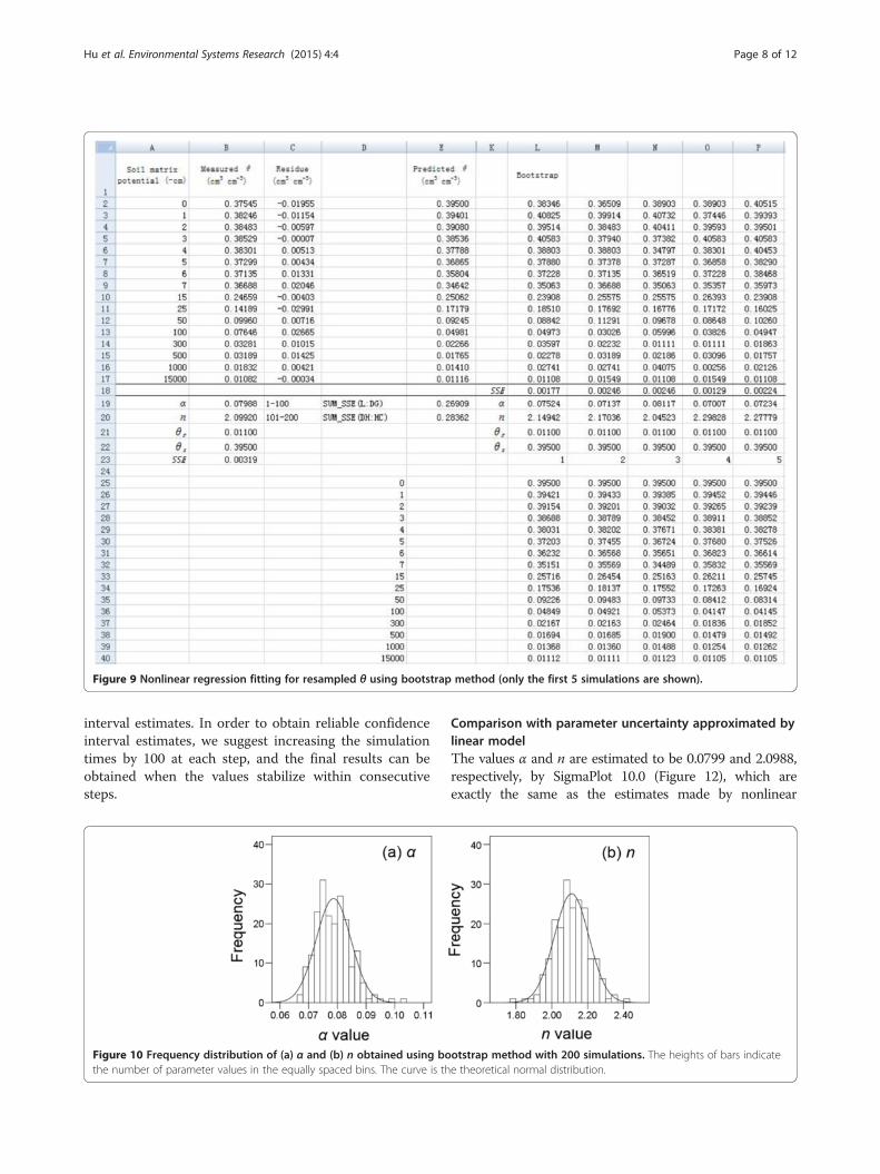
Figure 9 Nonlinear regression fitting for resampled θ using bootstrap method (only the first 5 simulations are shown).

Hu et al. Environmental Systems Research (2015) 4:4 Page 8 of 12

interval estimates. In order to obtain reliable confidenceinterval estimates, we suggest increasing the simulationtimes by 100 at each step, and the final results can beobtained when the values stabilize within consecutivesteps.

Figure 10 Frequency distribution of (a) α and (b) n obtained using bothe number of parameter values in the equally spaced bins. The curve is th

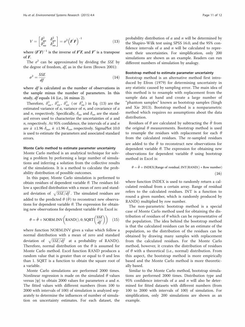
Comparison with parameter uncertainty approximated bylinear modelThe values α and n are estimated to be 0.0799 and 2.0988,respectively, by SigmaPlot 10.0 (Figure 12), which areexactly the same as the estimates made by nonlinear

otstrap method with 200 simulations. The heights of bars indicatee theoretical normal distribution.

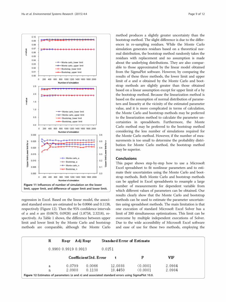
Figure 11 Influences of number of simulation on the lowerlimit, upper limit, and difference of upper limit and lower limit.

Hu et al. Environmental Systems Research (2015) 4:4 Page 9 of 12

regression in Excel. Based on the linear model, the associ-ated standard errors are estimated to be 0.0066 and 0.1138,respectively (Figure 12). Then the 95% confidence intervalsof α and n are (0.0670, 0.0928) and (1.8758, 2.3218), re-spectively. As Table 1 shows, the difference between upperlimit and lower limit by the Monte Carlo and bootstrapmethods are comparable, although the Monte Carlo

Figure 12 Estimates of parameters (α and n) and associated standard

method produces a slightly greater uncertainty than thebootstrap method. The slight difference is due to the differ-ences in re-sampling residues. While the Monte Carlosimulation generates residues based on a theoretical nor-mal distribution, the bootstrap method randomly takes theresidues with replacement and no assumption is madeabout the underlying distributions. They are also compar-able to those approximated by the linear model obtainedfrom the SigmaPlot software. However, by comparing theresults of these three methods, the lower limit and upperlimit of α and n obtained by the Monte Carlo and boot-strap methods are slightly greater than those obtainedbased on a linear assumption except for upper limit of α bythe bootstrap method. Because the linearization method isbased on the assumption of normal distribution of parame-ters and linearity at the vicinity of the estimated parametervalue, and it is more complicated in terms of calculation,the Monte Carlo and bootstrap methods may be preferredto the linearization method to calculate the parameter un-certainties in spreadsheets. Furthermore, the MonteCarlo method may be preferred to the bootstrap methodconsidering the less number of simulations required forthe Monte Carlo method. However, if the number of mea-surements is too small to determine the probability distri-bution for Monte Carlo method, the bootstrap methodmay be superior.

ConclusionsThis paper shows step-by-step how to use a MicrosoftExcel spreadsheet to fit nonlinear parameters and to esti-mate their uncertainties using the Monte Carlo and boot-strap methods. Both Monte Carlo and bootstrap methodscan be applied in Excel spreadsheets to resample a largenumber of measurements for dependent variable fromwhich different values of parameters can be obtained. Ourresults clearly show that the Monte Carlo and bootstrapmethods can be used to estimate the parameter uncertain-ties using spreadsheet methods. The main limitation is thatone execution of standard Microsoft Excel Solver has alimit of 200 simultaneous optimizations. This limit can beovercome by multiple independent executions of Solver.Due to the wide accessibility of Microsoft Excel softwareand ease of use for these two methods, employing the

errors using SigmaPlot 10.0.

Hu et al. Environmental Systems Research (2015) 4:4 Page 10 of 12

Monte Carlo and bootstrap methods in spreadsheets isstrongly recommended to estimate nonlinear regressionparameter uncertainties.In this paper, we demonstrated the methodology with

the van Genuchten water retention curve. The methodcan be applied to any mathematical functions or modelsthat can be evaluated by Excel. Therefore, the method-ology presented in this paper has wide applicability. Fur-ther, with little modification, the Monte Carlo methodor bootstrap method can be used in Microsoft Excel toestimate the uncertainty of hydrologic or environmentalpredictions with single or multiple input parametersunder different degrees of uncertainty.

MethodsSoil water retention curveSoil water content is a function of soil matric potential ψunder equilibrium conditions, and this relationship θ(ψ)can be described by different types of water retentioncurves. The soil water retention curve is a basic soil prop-erty and is critical for predicting water related environmen-tal processes (Fredlund et al. 1994). Among various soilwater retention curve models, the van Genuchten (1980)model is the most widely used one (Han et al. 2010). It ishighly nonlinear and can be expressed as:

θ ψð Þ ¼ θr þ θs−θrð Þ 1þ α ψj jð Þnð Þ−1þ1n ð5Þ

where θ(ψ) is the soil water content [cm3 cm−3] at soilwater potential ψ (−cm of water), θr is the residual watercontent [cm3 cm−3], θs is the saturated water content[cm3 cm−3], α is related to the inverse of the air entry suc-tion [cm−1], and n is a measure of the pore-size distribution(dimensionless). We measured θ(ψ) at 16 soil water poten-tials for a sandy soil using Tempe pressure cells (at soilmatrix potentials ranging from 0 to −500 cm) and pressureplates (at soil water potentials of −1000 and −15000 cm). θsis measured using oven drying method after saturation, andθr is estimated as water content of soil approaching air-dryconditions (Wang et al. 2002). θs and θr are 0.395 and0.011, respectively. Note that the soil water content (0.375)at zero matrix potential is lower than θs due to the soilwater movement under gravity. This paper will focus onthe estimation of parameters α and n and their associated95% confidence intervals.

Parameter uncertainty estimation by linearization ofnonlinear modelWe express the van Genuchten model (Eq. 5) as:

θi ¼ f β;ψi

� �þ εi ð6Þwhere θi is the i th observation for the dependent vari-able θ(ψ) (i = 1, 2, …16), ψi is the i th observation for thepredictor |ψ|. β is a vector of parameters which includes

parameters α and n. εi is a random error, which is as-sumed to be independent of the errors of other observa-tions and normally distributed with a mean of zero andvariance of σ2.The sum of squared residuals (SSE) for nonlinear re-

gression can be written as:

SSE βð Þ ¼X

θi−f β;ψi

� �� �2 ð7Þ

The model has the maximum likelihood when the SSEis minimized. Namely, when the partial derivative

∂SSE βð Þ∂β

¼ −2X

θi−f β;ψi

� �� � ∂f β;ψi

� �∂β

ð8Þ

is zero, parameters β are optimized. Once the optimumvalues of β are obtained, the parameter uncertainties canbe estimated by linearizing the nonlinear model functionat the optimum point using the first-order Taylor seriesexpansion method (Fox and Weisberg 2010).Let

Fij ¼∂f β̂;ψi

� �∂βj

ð9Þ

where β̂ is the optimized value, j refers to the jth of pa-rameters (j = 1, 2, and β1 = α, β2 = n).Assume matrix F = [Fij]. In our case,

F ¼

∂f β̂;ψ1

� �∂α

∂f β̂;ψ1

� �∂n

∂f β̂;ψ2

� �∂α

∂f β̂;ψ2

� �∂n

⋮ ⋮∂f β̂;ψ16

� �∂α

∂f β̂;ψ16

� �∂n

266666666664

377777777775

ð10Þ

where∂f β̂;ψið Þ

∂α and∂f β̂;ψið Þ

∂n can be calculated by the follow-ing formulae:

∂f β̂;ψi

� �∂α

¼ f α̂ þ Δα̂ð Þ; n̂;ψið Þ−f α̂−Δα̂ð Þ; n̂;ψið Þð Þ= 2Δα̂ð Þð11Þ

∂f β̂;ψi

� �∂n

¼ f α̂; n̂ þ Δn̂ð Þ;ψið Þ−f α̂; n̂−Δn̂ð Þ;ψið Þð Þ= 2Δn̂ð Þð12Þ

where Δ = 0.015, α̂ and n̂ are optimized value of α and n,respectively.The estimated asymptotic covariance matrix (V) of the

estimated parameters can be obtained by (Fox andWeisberg 2010):

Hu et al. Environmental Systems Research (2015) 4:4 Page 11 of 12

V ¼ δ2αα δ2αnδ2nα δ2nn

� �¼ σ2 F

0F

� �−1ð13Þ

where (F 0F)− 1 is the inverse of F 0F, and F 0 is a transposeof F.The σ2 can be approximated by dividing the SSE by

the degree of freedom, df, as in the form (Brown 2001):

σ2 ¼ SSEdf

ð14Þ

where df is calculated as the number of observations inthe sample minus the number of parameters. In thisstudy, df equals 14 (i.e., 16 minus 2).Therefore, δ2αα , δ

2nn , δ

2αn ( or δ2nα ) in Eq. (13) are the

estimated variance of α, variance of n, and covariance of αand n, respectively. Specifically, δαα and δnn are the stand-ard errors used to characterize the uncertainties of α andn, respectively. At 95% confidence, the intervals of α and nare α̂ ±1.96 δαα, n̂ ±1.96 δnn, respectively. SigmaPlot 10.0is used to estimate the parameters and associated standarderrors.

Monte Carlo method to estimate parameter uncertaintyMonte Carlo method is an analytical technique for solv-ing a problem by performing a large number of simula-tions and inferring a solution from the collective resultsof the simulations. It is a method to calculate the prob-ability distribution of possible outcomes.In this paper, Monte Carlo simulation is performed to

obtain residues of dependent variable θ. The residues fol-low a specified distribution with a mean of zero and stand-

ard deviation offfiffiffiffiffiffiffiffiffiffiffiffiffiffiffiffiSSE=df

p. The simulated residues are

added to the predicted θ (θ̂ ) to reconstruct new observa-tions for dependent variable θ. The expression for obtain-ing new observations for dependent variable θ in Excel is:

θ ¼ θ̂ þNORM:INV RANDðÞ; 0; SQRTSSEdf

� �ð15Þ

where function NORM.INV gives a value which follow anormal distribution with a mean of zero and standard

deviation offfiffiffiffiffiffiffiffiffiffiffiffiffiffiffiffiSSE=df

pat a probability of RAND().

Therefore, normal distribution on the θ is assumed forMonte Carlo method. Excel function RAND produces arandom value that is greater than or equal to 0 and lessthan 1. SQRT is a function to obtain the square root ofa variable.Monte Carlo simulations are performed 2000 times.

Nonlinear regression is made on the simulated θ valuesversus |ψ| to obtain 2000 values for parameters α and n.The fitted values with different numbers (from 100 to2000 with intervals of 100) of simulation is analyzed sep-arately to determine the influences of number of simula-tion on uncertainty estimates. For each dataset, the

probability distribution of α and n will be determined bythe Shapiro-Wilk test using SPSS 16.0, and the 95% con-fidence intervals of α and n will be calculated to repre-sent their uncertainties. For simplification, only 200simulations are shown as an example. Readers can rundifferent numbers of simulation by analogy.

Bootstrap method to estimate parameter uncertaintyBootstrap method is an alternative method first intro-duced by Efron (1979) for determining uncertainty inany statistic caused by sampling error. The main idea ofthis method is to resample with replacement from thesample data at hand and create a large number of“phantom samples” known as bootstrap samples (Singhand Xie 2013). Bootstrap method is a nonparametricmethod which requires no assumptions about the datadistribution.

Residues of θ are calculated by subtracting the θ̂ fromthe original θ measurements. Bootstrap method is usedto resample the residues with replacement for each θfrom the calculated residues. The re-sampled residues

are added to the θ̂ to reconstruct new observations fordependent variable θ. The expression for obtaining newobservations for dependent variable θ using bootstrapmethod in Excel is:

θ ¼ θ̂ þ INDEX Range of residual; INT RANDðÞ � Row numberð Þðð16Þ

where function INDEX is used to randomly return a cal-culated residual from a certain array. Range of residualrefers to the calculated residues. INT is a function toround a given number, which is randomly produced byRAND() multiplied by row number.The non-parametric bootstrap method is a special

case of Monte Carlo method used for obtaining the dis-tribution of residues of θ which can be representative ofthe population. The idea behind the bootstrap methodis that the calculated residues can be an estimate of thepopulation, so the distribution of the residues can beobtained by drawing many samples with replacementfrom the calculated residues. For the Monte Carlomethod, however, it creates the distribution of residuesof θ with a theoretical (i.e., normal) distribution. Fromthis aspect, the bootstrap method is more empiricallybased and the Monte Carlo method is more theoretic-ally based.Similar to the Monte Carlo method, bootstrap simula-

tions are performed 2000 times. Distribution type and95% confidence intervals of α and n will also be deter-mined for fitted datasets with different numbers (from100 to 2000 with intervals of 100) of simulation. Forsimplification, only 200 simulations are shown as anexample.

Hu et al. Environmental Systems Research (2015) 4:4 Page 12 of 12

Competing interestsThe author declares that there are no competing interests associated withthis research work.

Authors’ contributionsWH analyzed the data and wrote the draft. JX and HC participated in thedata analysis. BS designed the study. All authors read and approved the finalmanuscript.

Authors’ informationWei Hu is a professional research associate at the University of Saskatchewanand specialist for soil hydrology. Jing Xie is a PhD student in University ofSaskatchewan who is investigating legume fertilization. Henry Wai Chau is alecturer in environmental physics in Lincoln University. Bing Cheng Si is a fullprofessor in University of Saskatchewan and specializes in soil physics.

AcknowledgementsThe project was funded by the Natural Sciences and Engineering ResearchCouncil (NSERC) of Canada.

Author details1Department of Soil Science, University of Saskatchewan, Saskatoon, SK S7N5A8, Canada. 2Department of Soil and Physical Science, Lincoln University,PO Box 84Lincoln, Christchurch 7647, New Zealand.

Received: 22 January 2015 Accepted: 11 March 2015

ReferencesBerger RL (2007) Nonstandard operator precedence in Excel. Comput Stat Data

An 51:2788–2791Brown AM (2001) A step-by-step guide to non-linear regression analysis of

experimental data using a Microsoft Excel spreadsheet. Comp Meth Prog Bio65:191–200

Conedera M, Torriani D, Neff C, Ricotta C, Bajocco S, Pezzatti GB (2011) UsingMonte Carlo simulations to estimate relative fire ignition danger in alow-to-medium fire-prone region. Forest Ecol Manag 26:2179–2187

Cwiertny DM, Roberts AL (2005) On the nonlinear relationship between k(obs)and reductant mass loading in iron batch systems. Environ Sci Technol39:8948–8957

Delboy H (1994) A non-linear fitting program in pharmacokinetics with Microsoft®Excel spreadsheet. Int J Biomed Comput 37:1–14

Efron B (1979) Bootstrap method: another look at the Jackknife. Ann Stat 7:1–26Efron B, Tibshirani R (1993) An introduction to the Bootstrap. Champman & Hall,

London, UKFox J, Weisberg S (2010) Nonlinear regression and nonlinear least squares in R: An

appendix to an R companion to applied regression, second edition. http://socserv.socsci.mcmaster.ca/jfox/Books/Companion/appendix/Appendix-Nonlinear-Regression.pdf.

Fredlund DG, Xing AQ, Huang SY (1994) Predicting the permeability function forunsaturated soils using the soil-water characteristic curve. Can Geotech J31:533–546

Han XW, Shao MA, Hortaon R (2010) Estimating van Genuchten modelparameters of undisturbed soils using an integral method.Pedosphere 20:55–62

Harris DC (1998) Nonlinear least-squares curve fitting with Microsoft Excel Solver.J Chem Educ 75:119–121

Luo B, Maqsood I, Yin YY, Huang GH, Cohen SJ (2003) Adaption to climatechange through water trading under uncertainty - An inexact two-stagenonlinear programming approach. J Environ Inform 2:58–68

Singh K, Xie M (2013) Bootstrap: A statistical method. From Rutgers University.http://www.stat.rutgers.edu/home/mxie/rcpapers/bootstrap.pdf.

Smith LH, McCarty PL, Kitanidis PK (1998) Spreadsheet method for evaluation ofbiochemical reaction rate coefficients and their uncertainties by weightednonlinear least-squares analysis of the integrated Monod equation.Appl Environ Microbiol 64:2044–2050

Tong L, Chang C, Jin S, Saminathan R (2012) Quantifying uncertainty of emissionestimates in National Greenhouse Gas Inventories using bootstrapconfidence intervals. Atmos Environ 56:80–87

van Genuchten MT (1980) A closed-form equation for predicting the hydraulicconductivity of unsaturated soils. Soil Sci Soc Am J 44:892–898

Wang QJ, Horton R, Shao MA (2002) Horizontal infiltration method for determiningBrooks-Corey model parameters. Soil Sci Soc Am J 66:1733–1739

Wraith JM, Or D (1998) Nonlinear parameter estimation using spreadsheetsoftware. J Nat Resour Life Sci Educ 27:13–19

Submit your manuscript to a journal and benefi t from:

7 Convenient online submission

7 Rigorous peer review

7 Immediate publication on acceptance

7 Open access: articles freely available online

7 High visibility within the fi eld

7 Retaining the copyright to your article

Submit your next manuscript at 7 springeropen.com