Evaluation of Passive RFID System in a Dynamic Work Environment

by

SHRINIWAS AYYER

A thesis submitted to the

Graduate School – New Brunswick

Rutgers, The State University of New Jersey

in partial fulfillment of the requirements

for the degree of

Master of Science

Graduate Program in Electrical and Computer Engineering

written under the direction of

Professor Ivan Marsic

and approved by

___________________

___________________

____________________

____________________

New Brunswick, New Jersey

October 2012

ii

ABSTRACT OF THE THESIS

EVALUATION OF PASSIVE RFID SYSTEM IN A DYNAMIC WORK ENVIRONMENT

By SHRINIWAS AYYER

Thesis Director:

Professor Ivan Marsic

RFID has been one of the most widely used sensing technologies. Due to its ease of

integration, low cost and minimal system intervention required, a lot of domains are

deploying RFID for their applications. A major market of RFID technology applications has

been the inventory and tracking application. The data obtained from RFID, however, also

contains high level of information in it, which can be used and exploited for sensing

applications like localization, motion detection, activity recognition, etc. Despite, the

widespread use of RFID, there are some technical shortcomings and lack of a system design

approach which hinders the performance of RFID systems in dynamic and critical settings.

Our goal is to introduce the Passive RFID technology in a dynamic work environment like the

Trauma Resuscitation Bay as part of a context-aware system to support activity recognition.

Mobility of an object is closely related to its usage and hence the activity being performed.

iii

Detecting mobility of an object using passive RFID technology is the first step towards

activity recognition.

The deployment of the RFID system and the placement of the antennas play a crucial role in

the performance of their sensing application. In this work, we have devised a method to

determine the effectiveness of an RFID equipment setup. We have analyzed different RFID

setups and we discuss the metrics used to determine their effectiveness. We conducted

experiments with different scenarios to collect the data and evaluated the performance of a

setup in each scenario. The results obtained helped us to correlate the RFID setup with its

detection performance. We also ran a classification algorithm on the data collected and

evaluated the object motion detection accuracy for all the set ups. Our work provides a

ground rule for the RFID set up requirements to be considered for detection applications

and also provides insights into the features that can be used for state classification of

objects using the RFID data.

iv

Dedication

To My Parents

v

Acknowledgment

I would like to thank Professor Ivan Marsic for allowing me to work on this highly engaging

project. I would like to thank him for all the guidance and constant feedback and also for

inspiring me throughout. I would like to thank Siddika Parlak for helping me in this project

and her guidance. I would also like to thank my friends who have helped me in conducting

the experiments. Without their help, we could not have collected reliable RFID data. Finally,

I would like to thank my parents without whose support and motivation all this would not

have been possible.

vi

Contents Abstract ……………………………………………………………………………………………………………………………. ii

Dedication ………………………………………………………………………………………………………………………… iv

Acknowledgment ………………………………………………………………………………………………………………. v

1. Introduction……………………………………………………………………………………………………………………. 1

1.1 Motivation ……………………………………………………………………………………………………….. 1

1.2 Contribution of the thesis ………………………………………………………………………………… 3

2. RFID Technology ……………………………………………………………………………………………………………. 5

2.1 Introduction ……………………………………………………………………………………………………. 5

2.2 RFID Technology: Advantages and Challenges …………………………………………………. 7

2.3 RFID Equipment and Environmental Setting ……………………………………………………. 8

3. Evaluation of RFID Equipment Set Up …………………………………………………………………………… 14

3.1 Introduction …………………………………………………………………………………………………… 14

3.2 Criteria for evaluating the goodness of a setup ……………………………………………… 16

3.3 Experimentation Methodology ……………………………………………………………………… 19

3.4 Antenna Placement ………………………………………………………………………………………. 21

3.5 Antenna Placement Results …………………………………………………………………………… 29

3.6 Tag Placement ………………………………………………………………………………………………. 43

3.7 Tag Placement Results …………………………………………………………………………………… 48

3.8 Summary ………………………………………………………………………………………………………. 52

4. Object State Detection ………………………………………………………………………………………………… 54

4.1 Data Collection ……………………………………………………………………………………………… 55

4.2 Classification Methodology …………………………………………………………………………… 56

4.3 Classification Results …………………………………………………………………………………….. 59

4.4 Summary ………………………………………………………………………………………………………. 64

5. Conclusion and Future work ……………………………………………………………………………………….. 66

5.1 Conclusion ……………………………………………………………………………………………………. 66

5.2 Future Work …………………………………………………………………………………………………. 66

References ……………………………………………………………………………………………………………………… 68

vii

List of Tables

Table 2.1 RFID Reader Specifications ……………………………………………………………………………… 10

Table 2.2 RFID Reader External Circular Polarized Antenna Specifications ……………………… 11

Table 2.3 Passive RFID Tag Specifications ……………………………………………………………………….. 12

Table 3.1 Location Change Experiment Read Rate Values ………………………………………………. 30

Table 3.2 Location Change Experiment Mahalanobis Distances ……………………………………… 32

Table 3.3 Classification Accuracy for Location Change Experiments ……………………………….. 33

Table 3.4 Motion Detection Experiments Read Rate Values …………………………………………… 35

Table 3.5 Motion Detection Experiments Mahalanobis Distances ………………………………….. 36

Table 3.6 Classification Accuracy for Motion Detection Experiments ……………………………… 38

Table 3.7 Location Change Experiment Results – Additional Scenarios …………………………… 41

Table 3.8 Motion Detection Experiment Results – Additional Scenarios …………………………. 42

Table 3.9 Tag Placement Results – Material of the object ………………………………………………. 48

Table 3.10 Tag Placement Read Rate Values for scenario 2 ……………………………………………. 49

Table 3.11 Tag Placement Read Rate Values for scenario 3 ……………………………………………. 50

Table 3.12 Tag Placement scenario 4 – Read Rate and Mahalanobis Distance Values …….. 52

viii

List of Illustrations

Figure 2.1 Experimental Lab Setup – Top View ………………………………………………………………… 9

Figure 2.2 Alien ALR 9900 RFID Reader ……………………………………………………………………………. 11

Figure 2.3 Alien ALR 9611 CR Antenna …………………………………………………………………………….. 12

Figure 2.4 The squiggle passive RFID Tag …………………………………………………………………………. 13

Figure 3.1 Location Change Experiment …………………………………………………………………………… 21

Figure 3.2 Motion Experiment …………………………………………………………………………………………. 21

Figure 3.3 Trauma Bay Zones …………………………………………………………………………………………… 22

Figure 3.4 Top View of five different antenna setups ………………………………………………………. 24

Figure 3.5 Read Rate Values for Location Change Experiments ……………………………………….. 31

Figure 3.6 Mahalanobis Distance Values for Location Change Experiments …………………….. 33

Figure 3.7 Classification Accuracy Values for Location Change Experiments ……………………. 34

Figure 3.8 Average Read rates for Motion Detection Experiments ………………………………….. 36

Figure 3.9 Mahalanobis Distance Values for Motion Detection Experiments ………………….. 37

Figure 3.10 Classification Accuracy for Motion Detection Experiments …………………………… 39

Figure 3.11 Objects used for Tag Placement Experiments ……………………………………………….. 44

Figure 3.12 Read Rate Curve for tags attached on a liquid container ………………………………. 48

Figure 3.13 Read Rate Graphs for Tag Placement Experiments – Multiple Tagging …………. 49

Figure 3.14 Read Rate Graphs for Tag Placement Experiments – Tag Folding …………………. 51

Figure 4.1 Location Change Classification Accuracy (in percentage): Decision Tree Classifier

and varying window lengths and slide lengths ……………………………………………………………….. 60

Figure 4.2 Location Change Classification Accuracy (in percentage): Support Vector Machine

Classifier and varying window lengths and slide lengths ………………………………………………. 61

Figure 4.3 Location Change Classification Accuracy (in percentage): Random Forest Classifier

and varying window lengths and slide lengths ………………………………………………………………. 61

ix

Figure 4.4 Motion Detection Classification Accuracy (in percentage): Decision Tree Classifier

and varying window lengths and slide lengths …………………………………………………………… 62

Figure 4.5 Motion Detection Classification Accuracy (in percentage): Support Vector

Machine Classifier and varying window lengths and slide lengths ……………………………… 63

Figure 4.6 Motion Detection Classification Accuracy (in percentage): Random Forest

Classifier and varying window lengths and slide lengths ……………………………………….……. 63

Figure 4.7 Mahalanobis Distance Average over the number of antennas versus Classification

Accuracy – all five RFID setups ……………………………………………………………………………..……. 65

1

Chapter 1: Introduction

1.1 Motivation

A lot of technological advancements have been made in the fields of voice recognition,

gesture recognition, emotion detection opening up a lot of prospective areas of research for

improving the safety and quality of patient care. Among these, radio-frequency based

identification is most promising given its unobtrusiveness and easy integration into the

healthcare systems. Other advantages of RFID over other sensing technologies include low

cost, no line of sight requirements, minimal human intervention. Initial attempts to deploy

information systems to aid trauma teams have been promising, but have shown limited

usability.

RFID technology is widely used in inventory tracking, access control systems, vehicle

identification, ticketing, etc. All these application domains focus on item level tracking

where the main aim is to detect the object. In a healthcare domain, item level detection will

not be of any significant use if the state of the object or the location of an object is not

known. Developing a context aware system in a trauma room requires state identifications

like mobility detection of objects, usage detection and also the information regarding the

location of the object. All these things will contribute to determine the current activity being

conducted in the trauma room. Unlike item level tracking where a signal from a particular

tag is enough to identify the presence of the object, all these identifications require high

level information from the RFID data being extracted at the reader, rather than just

identifying the tag as present or not present.

2

Introduction of these identification techniques with Passive RFID technology in a dynamic

and time critical environment like the trauma resuscitation room is very challenging due to

several reasons. Firstly, trauma rooms are crowded with many people moving around

causing a lot of interference. Secondly, there are many medical objects in use at the same

time reducing the detecting capabilities of the readers. Thirdly, the position of the tag on

the object matters since if the tag gets covered during usage, then the reader will not be

able to detect it. Fourth, medical tools are made of different materials and some object

contains liquids affecting the radio signals. Fifth, certain objects come with a plastic packing

and hence the tags can only be placed on the plastic cover. Once the cover is removed, the

object can no longer be tracked. Lastly, due to the shape of certain medical objects e.g.

stethoscope, it becomes difficult to place the tag properly on the object so that it emits

sufficient radio signal back and is getting detected.

Thus, with a lot of potential for the RFID technology in the field of healthcare, there is not

enough work done to develop a set of rules, guidelines to follow to deploy an RFID system in

the healthcare domain and get satisfactory results. Our aim is to introduce the passive RFID

technology in a trauma resuscitation bay as a part of a future context-aware system to track

the activities of a trauma room [6].

3

1.2 Contribution of the thesis

RFID technology can be used for inferring high level information, such as motion, location or

activity. However passive RFID technology is affected by external interferences as well as a

lot of other factors like multipath propagation, inter tag collision, human interference, etc.

The Received Signal Strength Indicator (RSSI) can be very noisy even when both the tags and

readers are stationary. Hence, for reliability, generally multiple readers or multiple antennas

with a single reader are used. Currently, number and placement of antennas, as well as tags,

is determined based on heuristics, which aims to maximize the read rate or the accuracy. A

lot of work has been done previously [1, 2, 3] on the read rates obtained from an RFID set

up and is focused on improving the coverage area/read range for a given system. No work is

done so far on optimizing the RFID setup considering the motion detection or activity

detection application using an RFID system. Read rates are not that intuitive and for motion

detection or activity recognition, we need to extract high level features from the received

signal.

It is important to note that RFID is a unique sensing technique which uses the wireless link

to communicate the information. Hence it differs from other sensors in being sensitive to

tag orientation, antenna orientation, antenna placement and other setup parameters. In

our thesis, we develop a setup evaluation method based on distribution distance, and apply

our method to human activity recognition in a dynamic medical setting, an example of

which is trauma resuscitation. Our thesis explains the techniques to follow and the metrics

to consider for RFID set up evaluation in an application domain where state recognition is

used.

4

Our long term goal of the project being activity recognition in a trauma resuscitation room,

we simulated a trauma bay in our research lab and conducted motion detection and

location change experiments. We developed an algorithm for classification and evaluated

the accuracy for different set ups, and by changing different parameters. In our work, we

also explore the problem of long-range object motion detection using passive RFID. Our

work focuses on dynamic settings suffering interference caused by humans and multiple

tags. We observed that, the change in signal due to actual tag motion and the variations in

signal due to external interferences are separated and distinguishable using statistical

methods.

We extract descriptive features from the received signal at the reader and classify them

using machine learning techniques. In our thesis, we have reported the experimental results

obtained with several statistical features and classifiers.

Thus, the contribution of our thesis is twofold - First, we perform experimental verification

and evaluation of RFID setups to determine the most optimum set up for the domain of

object state classification. Second, we perform classification of the object state for the

different RFID setups and analyze the results.

5

Chapter 2: RFID Technology

2.1 Introduction

Radio Frequency Identification (RFID) is the use of an object (typically referred to as an RFID

tag) applied to or incorporated into a product, animal, or person for the purpose of

identification and tracking using radio waves. RFID simply extracts the data present in the

memory chip and makes it available for further processing.

A basic RFID system consists of three components:

a) An antenna or coil

b) A transceiver (with decoder)

c) A transponder (RF tag) electronically programmed with unique information more often a

serial number unique for that tag.

There are many different types of RFID systems available in the market. These are

categorized according to their frequency ranges. Some of the most commonly used RFID kits

are as follows:

1) Low-frequency (30 KHz to 500 KHz)

2) Mid-Frequency (900 KHz to 1500MHz)

3) High Frequency (2.4GHz to 2.5GHz)

These frequency ranges mostly tell the RF ranges of the tags from low frequency tags

ranging from 3m to 5m, mid-frequency ranging from 5m to 17m and high frequency ranging

up to 200m.

With RFID, the electromagnetic or electrostatic coupling in the RF (radio frequency) portion

of the electromagnetic spectrum is used to transmit signals. An RFID system consists of an

antenna and a transceiver, which reads the radio frequency and transfers the information to

6

a processing device (reader) and a transponder or RF tag, which contains the RF circuitry

and information to be transmitted. The antenna provides the means for the integrated

circuit to transmit its information to the reader that converts the radio waves reflected back

from the RFID tag into digital information that can be passed on to computers that can

analyze data.

There are three types of RFID technology:

1) Active RFID Technology - Active RFID tags are typically larger and more expensive to

produce, since they require a power source. Active RFID tags broadcast their signal

to the reader, and are typically more reliable and accurate than passive RFID tags.

Since active RFID tags have a stronger signal, they are more adept for environments

that make it hard to transmit other types of tags, such as under water, or from

farther away.

2) Passive RFID Technology - Passive RFID tags, on the other hand, do not have internal

power supplies and rely on the RFID reader to transmit data. A small electrical

current is received through radio waves by the RFID antenna, and power the CMOS

just enough to transmit a response. Passive RFID tags are more suited for

warehousing environments where there is not a lot of interference, and relatively

short distances (typically ranging anywhere from a few inches to a few yards). Since

there is no internal power supply, passive RFID tags are much smaller and cheaper

to produce.

7

3) Semi-Passive RFID Technology - Semi-passive RFID tags are similar to active RFID

tags in that semi-passive RFID tags have an internal power supply, but they do not

broadcast a signal until the RFID reader transmits one first.

2.2 RFID Technology: Advantages and Challenges

RFID is one of the most widely used sensing technologies. In our work, we are using the

passive RFID technology in the trauma room for detecting usage because of some of its

advantages.

Compared to the widely used barcode system, RFID does not require line of sight

link with the reader.

Passive RFID tags are cheaper and can be easily deployed on any object.

Unlike, computer vision, RFID tags are easily re-programmable and hence no

permanent data is maintained.

RFID technology enables faster and easier detection of multiple tags simultaneously.

It does not require focused passing of sensors over the scanners, thus minimizing

human interference.

Due to its passive nature, it also has certain disadvantages compared to other sensors:

It is sensitive to the environment in which it is deployed. External factors such as

metallic cabinets, human intervention cause a lot of interference in the signal.

It is also affected by the material of the object on which it is tagged; we need special

tags for metals and liquid containers.

8

It has a limited read range due to its backscatter mechanism. Due to the absence of

an external power source, it cannot be detected over long distances.

2.3 RFID Equipment and Environmental Setting

We are performing our experiments in a lab room which is partially filled with furniture like

metal cabinets, wooden desks ad separators, which caused multipath fading and distortion

of RF signal. We have tried to simulate a setting similar to the trauma bay [Figure 2.1] in the

lab room, with a patient bed in the center, side furniture and free space. A tagged object

was interacted near the patient bed and this area was our focus of attention throughout the

experiments. We performed two distinct set of experiments: Set one - with respect to the

RFID setup evaluation. Set two - with respect to the motion detection classification analysis.

We have used off the shelf RFID equipment from Alien [4]: an RFID reader (ALR-9900),

circularly polarized antennas (ALR – 9611 – CR) and passive tags (Squiggle ALN-9540). The

number of antennas and the antenna setup varied according to the experimenting sets.

Regardless of the number of tags used in any experiment, the reader scanned for multiple

tags in the environment, rather than a fast search for the single tag. The readers were

operated in a dense reader mode (DRM), which prevents interference among readers, to

obtain results scalable to larger deployments with multiple readers. Also, DRM yields the

best performance when tag-to-reader distance is greater than 1.5 meters. Radio signal was

emitted in a round robin fashion through one antenna at a time (for 0.5 seconds). The

reader emitted 1 watt of RF power. The number of readers used in an experiment depended

upon the number of antennas used in the experimental set up. Only three antennas were

9

connected to a reader. So for experiments dealing with more than three antennas, two

readers were used.

The experiments were conducted in a closed lab (Figure 2.1) which had multiple sources of

interferences like desks, glass cabinets, metal cabinets etc. A wooden cart was used as a

patient bed on which the RFID tagged object was placed during the experiments.

Figure 2.1: Experimental Lab Setup – Top View

Table

Cart 2

RFID Tagged Object

Desk

Desk Desk

Metal Cabinet

Glass Cabinet

Desk

Desk

Metal Cabinet

Desk

Reader

Metal

Cabinet

Metal

Cabinet

Desk

Table

Cart 1

10

Table 2.1: RFID Reader Specifications

Name Alien Multi-Port General purpose RFID Reader

Model Number ALR 9900

Architecture Point-to-multipoint reader network, mono-static antenna

Operating Frequency 902.75 MHZ – 927.25 MHZ

Hopping Channels 50

Channel Spacing 500 KHZ

Channel Dwell Time < 0.4s

RF Transmitter < 30 dBm at the end of 6 m LMR-195 cable

Modulation method Phase Reversal – Amplitude Shift Keying (ASK)

20 dB Modulation

Bandwidth

< 100 KHZ

RF Receiver 2 channels

Power Consumption 30 watts

Communications Interface RS-232 (DB-9 F), TCP/IP (RJ-45)

Inputs/Outputs 4 coax antenna, 4 inputs/8 outputs (optically isolated), RS-232 com port,

LAN, power

Dimensions 8* x 7* x 1.6*

Weight Approximately 1 kg

Operating Temperature -20oC to + 50

oC

LED indicators Power, Link, Active, Ant0-3, CPU, Read, Sniff, Fault(Red)

Software Support APIs, sample code, executable demo app(Alien Gateway)

Protocol Support Comply with EPC Class 1 Gen 2 and 18000 -6C

Compliance Certifications FCC Part 15;FCCID;P65ALR9900IOC:4370A-ALR9900

11

Figure 2.2: Alien ALR 9900 RFID Reader

Table 2.2: RFID Reader External Circular Polarized Antenna Specifications

Model ALR-9611-CR and ALR-9611-CL

3 dB Beamwidth E plane: 65o , H plane: 65

o

Frequency 902-928 MHZ

Gain (dB) 6.0 dBiL (maximum)

Polarization Circular

RF connector 6 m LMR-195 with reverse polarity

VSWR 1.5:1

Dimensions 8.5 x 10.5 x 1.65 (inches)

Weight .57 kg

12

Figure 2.3: Alien ALR 9611 CR Antenna

Table 2.3: Passive RFID Tag Specifications

IOC/IEC 18000-6C

EPCglobal Class 1 Gen 2

Integrated Circuit Alien Higgs-3

EPCglobal Certificate 950110126000001084

Operating Frequency 840-960 MHz

EPC Size 96-480 Bits

User Memory 512 Bits

TID 32 Bits

Unique TID 64 Bits

Access Password 32 Bits

Kill Password 32 Bits

13

Figure 2.4: The squiggle passive RFID Tag

14

Chapter 3: Evaluation of RFID Equipment Set Up

3.1 Introduction

The RSSI data obtained from the reader contains a lot of high level information which can be

used for inferring the state of the object. The RSSI or read rate can be very noisy even when

both the reader and antenna are static. For reliability, multiple antennas and tags must be used.

Currently, there is no specific protocol or guideline that could be used for the RFID system

design from a state recognition point of view. The RFID system usually gets deployed in a

manner that maximizes the coverage area and guarantees a respectable read rate [2, 3]. Read

rates are not always indicative for inference of high-level information. Accuracy, on the other

hand, depends on the methods used for data processing such as features and classifiers

selected. Current practice is placing antennas in a regular grid based on intuitions without

performing controlled experiments, optionally performing preliminary experiments to find the

best placement. Or using different styles and discussing their usefulness after performing all

experiments.

Although optimum placement problem arises for other sensors as well, passive RFID has two

properties that make the problem different: 1) Sensing components 2) Sensitivity. Most sensors

(e.g., accelerometers, temperature sensors and humidity sensors) have a single component for

sensing. Wireless communication is used only for transmitting to or receiving data from other

devices, such as a data processing unit. In case of RFID (as well as Wi-Fi), both sensing and data

transmission is performed via the wireless communication signal. Therefore the sensing system

consists of two components: sensors on objects (tags) and readers (base stations). The

deployment strategy must consider both components, possibly in conjunction.

15

Second, RFID is very sensitive to orientation and interference due to human occlusion and

movement. The received signal strength changes with the change in orientation of the tag

placed on the object. This might result in false positives or missed reads. RSSI (Received Signal

Strength Indicator) is also affected by the presence of human in the environment. Both these

factors are quite common to occur in a trauma resuscitation room.

In this chapter, we will explain about the setup evaluation method we developed based on

distribution distance, and apply our method to human activity recognition in a dynamic medical

setting, an example of which is trauma resuscitation. First, we list the requirements for antenna

and tag deployments in a trauma resuscitation setting. Next we define our criteria for evaluating

the goodness of placement, along with the other two criteria: read rate and accuracy. Then, we

discuss the results obtained from our experimentation and the defined metrics used.

There are two main components in an RFID set up which determine the performance of the set

up – Antenna Placement and Tag Placement. Antenna placement refers to the positioning of the

antenna in the system so as to transmit and receive the signals. Improper positioning of

antennas might lead to reduced coverage area, overlapping of antenna regions, missed

readings. Tag placement refers to the positioning of tag on the object. Since the positioning of

the tag on the object depends upon the object itself, we experimented with several different

medical objects with different tag positions on them.

Thus to evaluate an RFID equipment setup, we performed two types of experiments – antenna

experiments and tag experiments.

16

3.2 Criteria for evaluating the goodness of a setup

In this section, we describe our criteria for evaluating the goodness of deployment and discuss

their relation. Since, we performed two kinds of experiments in analyzing the optimum RFID

setup; we need to use the appropriate criterion for evaluating each experiment type.

3.2.1 Read Rate

Read rate has been defined in different ways in the literature depending on the use case. Our

goal of object-use detection requires a substantial amount of data from each tag to obtain

reliable results. Accordingly, we define read rate as the number of responses obtained from a

tag per unit of time. Read rate is simple to calculate and provides the basic high-level

information about the goodness of deployment. Most of the prior work [1, 2, 3] has evaluated

their RFID system performance in terms of read rate.

3.2.2 Distribution Distance

The RFID system deployment strategy usually focuses on the read rates of the tags. High

read rates are desirable and good, but they are not good indicators of usage. An object

standing still near to the reader will give good read rates compared to an object in use but

at a distance away from the reader. Hence we need to study the RSSI pattern obtained from

the signals to infer their usage. Distribution distance is one such feature which helps to

determine the usage by detecting the change in the pattern. Distribution distance is nothing

but the difference between the distributions of two signals. When an object is in use, the

RSSI pattern received at the reader is more fluctuating and varies a lot. Hence, the standard

deviation of the signal is higher when the object is in use. Thus the RFID setup should be

17

such that it complements the standard deviation when the object is in use. For example –

Suppose there are two available set ups A and B. We conduct an experiment in both the set

ups where a tagged object is not in use for the first 10 seconds and then used for the next

10 seconds. Now, we calculate the standard deviation of the data collected in the entire 20

seconds for both the set ups - stdA and stdB. We need to select the set up which is more

sensitive to the tag activity i.e. with higher standard deviation. If stdA > stdB, then set up A

will be the set up of our choice. Thus usage is very closely related to the standard deviation

of the signals which in turn is related to the distribution distances of the signals. Higher the

distribution distance, farther apart the signal patterns are, greater is the standard deviation.

In other words, distribution distance helps us to determine the sensitivity of an RFID set up

to location changes, motion, and usage of the tagged objects.

We calculate the distance between two RSSI patterns as follows: Let Xp is the RSSI sequence

generated when the tag is in one state (e.g., standing still), and Xq is the RSSI sequence

generated when the tag is in another state (e.g., in motion). We assume Xp and Xq are

generated by normal probability distributions P and Q, respectively, which are modeling

object’s state of motion. Mahalanobis distance is one such tool which is most commonly

used for calculating the difference between two distributions.

Mahalanobis Distance: Mahalanobis distance is a measure of similarity between a vector

and a set of vectors characterizing a distribution. Unlike the Euclidean distance, it takes the

correlations between variables into account and it is scale invariant (does not change when

variables are multiplied with a common factor). Formally, Mahalanobis distance of a

18

multivariate vector p to a multivariate distribution Q with mean µ and covariance S is

calculated as:

)()(),( 1 pSpQpd T

M

(1)

To find the distance between distributions P and Q, we define the following distance metric,

which favors high inter-distribution distance and low intra-distribution distance:

(2)

Where is defined as the average distance of samples in P to samples in Q:

n

i

im Qpd1

),( (3)

The Mahalanobis distance metric is closely related to separability of classes in a

classification problem: as the average inter-class distance increases and the average intra-

class distance decreases, i.e. classes are more separable, classification performance is

expected to improve. We used mahalanobis distance as a distribution distance metric

because of its advantages:

It automatically accounts for the scaling of the coordinate axes

It corrects for correlation between the different features

It can provide curved as well as linear decision boundaries

Compared to read rate, distribution distance better characterizes the distinguish ability of

object states for different RFID equipment setups. However it is a more complex measure

19

that requires selecting a distance metric and making assumptions on the data (e.g., normal

distribution), both of which may bias the judgment on the goodness of an RFID setup.

3.2.3 Use Detection Accuracy

Use detection accuracy represents the similarity between the hypothesis about object use

and the ground truth; therefore it is the direct measure to evaluate the goodness of a setup.

Several metrics can be used to measure the similarity between the hypothesis and the

ground truth, such as precision, F-score or classification accuracy [5]. In this work, we focus

on two cues indicating object use: coarse-level location and motion status. We formulate

both coarse-level localization and motion detection problems as classification problems and

calculate the classification accuracy as follows:

(4)

Calculating the accuracy requires building a recognition system, which includes feature

extraction, model training and classification steps. It measures the setup goodness in the

context of the end application; however, unlike read rate, which can be measured directly,

measuring accuracy requires building the entire end application system. Also, the overall

results may be biased by the selection of recognition system components.

3.3 Experimentation Methodology

Experiment – It basically means the collection of data performing multiple runs of the RFID

reading for a given environmental set up and tag set up. Each run of an experiment lasted

20 seconds and 5 runs were performed for each experiment. So we had 100 seconds of

20

data for each experiment. This might look small amount but our main aim was to

determine the best RFID set-up that could be used for efficient mobility detection

assuming the mobility detection algorithm has already been equipped.

Since the target audience of our mobility detection project was healthcare domain, we

wanted to simulate the environment of a typical surgery room in our lab. We used two

wooden carts to act as the patient beds and also surgical equipments were our object of

use. Our methodology can be broadly classified into two types:

1) Antenna Experiments

2) Tag Experiments

Both the types of experiments had several settings under them which will be explained in

detail later. The above classification of the experiments is based on the RFID equipment

itself which includes the antennae and the tags. We also performed experiments from the

usability point of view. Location estimation and mobility being the two most important

applications of RFID, we performed each experiment for both location change of the object

as well as the mobility.

Location change – These experiments basically meant changing the location of the

object after a specified time in an experimental run (figure 3.1). Since each run we

performed lasted 20 seconds, we changed the location of the object after 10

seconds. We performed this by using two wooden carts separated by a distance of

2m. The object was kept on one cart for 10 seconds and moved to the other cart

21

after 10 seconds. This perspective was used to simulate the scenario where the

objects are being moved from one place to the other during its use.

Figure 3.1: Location Change Experiment

Mobility – Mobility experiments were performed by using the objects and moving

them around after they have been stationary for a while (figure 3.2). The objects

were stationary for the first 10 seconds of the run and after that they moved around

(in close vicinity of the cart on which it was initially kept). This simulated the practice

when a person uses particular equipment which was kept on storage or on the table

for a while.

Figure 3.2: Motion Experiments

The object that was used for these experiments is a rectangular cardboard box that is

closed from all the sides. The dimensions of the box would be ~ 7 in * 3 in* 3 in. The lab is a

closed lab and has many interfering sources like the walls, separators and metallic cabinet.

3.4 Antenna Placement

The trauma bay consists of specific zones in which the objects are concentrated and used

(figure 3.3). It is very important to have proper coverage in these zones. In this section, we

Object at Cart A

(first 10 seconds)

Object at Cart B

(next 10 seconds)

Object standing still at Cart A

(first 10 seconds)

Object in motion at Cart A

(next 10 seconds)

22

list the requirements to be met for antenna placement. Next we show the different

antenna setups we experimented. Finally we discuss the results obtained for these setups

using the distribution distances and also talk about the optimum setup that is preferred for

our application.

3.4.1 Antenna Placement Requirements

We analyzed the trauma resuscitation setting focusing on the spatial distribution of objects

and identified five main zones where objects are usually located: patient-bed zone, right

and left zones, and foot and head zones (Figure 3.3). Objects are often stored, or left idle,

in left, right, head and foot zones. Objects cross inter-zone areas when they are relocated

for use in the patient-bed zone. Based on our analysis of a typical trauma setup [6], we

have come up with the following requirements for the antenna placement:

Figure 3.3: Trauma Bay Zones

23

For an optimal antenna placement, each zone must be under coverage of at

least one antenna. Remaining areas outside the zones need not be covered

because non-uniform object concentration of the trauma bay allows for non-

uniform antenna coverage.

Antennas must be placed such that their reception is minimally affected by the

object’s orientation.

The interference due to human presence and movement should be minimal.

The antennas should not hinder providers’ movements and task performance.

The number of deployed antennas should be minimized to reduce the cost of

the equipment and the interference between antennas, and to meet the

esthetical requirements.

Based on these requirements, we have come up with 5 different antenna setups which are

discussed in the following section.

3.4.2 Antenna Setup Experiments

1) Experimental Setup

During trauma resuscitation, medical objects appear either on patient-bed or in one of the

storage places (left, right, head and foot zones). We created a prototype environmental

setting in our laboratory including only two zones: the patient-bed zone (usage area, Z1 in

Figure 3.4) and the left zone (storage area, Z2 in Figure 3.4). Each zone contained a 0.9 m

tall cart. The carts were separated between 0.8-2.3 m away from each other, depending on

24

the experimental scenario. A cardboard rectangular box was tagged with an RFID tag and

handled by the experimenter as the target object.

Figure 3.4: Top view of five different antenna setups – Z2 represents the patient-bed zone and Z1 represents the left

storage zone. Ceiling-mounted antennas are shown with circles; angled antennas are shown with triangles.

Set Up 1: One ceiling mounted antenna placed between the two carts

As seen in the figure 3.4, this particular setting employs one ceiling mounted antenna

placed at the center of the two carts at a height of 2.7m above the cart. The antenna field

around each cart is identical not accounting for the interference due to other sources

nearby the carts. The area covered by this antenna was determined based on the antenna

radiation pattern provided by the vendor. We made a conic beam approximation (a cone

with its vertex on the transmitting antenna and its axis along the transmission direction) for

the directional radiation pattern of the antenna. The 3 dB beam width (65 degrees), also

specified by the vendor (Table 2.2), was used as the aperture angle of the cone. The

resulting coverage area for an antenna was a circle with a radius of 1.5 m at the height of

carts (distance of 1.8 m from the antenna). The coverage area of the antenna in this setup

included both storage and usage zones, meeting the coverage requirement (Req. #1).

25

Set Up 2: Two Ceiling mounted antennas placed one directly above each cart

This setting uses two ceiling mounted antennae one above each cart. The distance between

the two antennas is approximately the same as the distance between the two carts (figure

3.4).

Set Up 3: Two ceiling antennas perpendicular to the carts

There are two ceiling mounted antennae placed perpendicular to the line joining the

centers of the two carts. The distance between the two antennae is approximately equal to

the distance between the two carts which is around 2m (figure 3.4).

To increase the diversity of signals received from a tag, as well as to account for the

variability in object and tag orientation (Req. #2), we mounted the new antennas to

sidewalls such that they transmit through a different (ideally perpendicular) direction with

respect to the existing antennas (ceiling-mounted). Assuming an average human height of

1.7 m, we positioned the new antennas at a height of 2 m to reduce interference due to

human presence (Req. #3), and to minimize the obstruction of equipment on providers’

activities (Req. #4). To cover the experimental area, we also slanted the antennas to make

60˚ to the floor.

Set Up 4: Two antennae per zone

There is one ceiling mounted antenna and one side antenna for each cart. Placing of

multiple antennas for each zone basically helps in addressing different tag orientations. The

antennae in a zone should transmit in different directions. Set up 4 is a modification of set

up 2 with two additional side antennae (figure 3.4).

26

Set Up 5: Three antennae per zone

There is one ceiling antenna right above the cart and additional two side antennae. The two

side antennae are placed in such a way that they are radiating in perpendicular directions.

Thus this set up involves a total of 6 antennae and accounts more for different tag

orientations. However, interference between the antennae will also be high in this case due

to the close proximity of the antennae (figure 3.4).

2) Experimental Scenarios

In a dynamic environment like the trauma bay, there are a lot of scenarios which can affect

the performance of a given antenna setup [6]. On the basis of the antenna placement

requirements and our study of the trauma bay [6], we tested each setup with a list of

possible scenarios.

The scenarios simulated the environmental characteristics of trauma resuscitation that may

affect propagation of RFID radio signals.

Scenario #1: Stationary environment: This is the baseline scenario without any

environmental factors introduced.

Scenario #2: Deviations in zone locations: Although coarse-level zone locations in the

trauma bay are fixed (e.g., cabinets and counter along the walls, patient bed in the center of

the room), the patient bed and carts may slightly move during the resuscitation. Also, the

height of the patient bed is adjustable. To simulate these deviations in zone locations, we

moved the zones (i.e. carts) in the following directions:

27

2-a) Z1 and Z2 moved 0.6 m to north (distance between the zones remained constant).

2-b) Z1 moved 0.6 m to north; Z2 moved 0.6 m to south (distance between zones increased

to about 2.3 m).

2-c) Z1 moved 0.6 m to east; Z2 moved 0.6 m to west (distance between zones decreased to

0.8 m).

Scenario #3: Changes in object orientation: Object’s tag in the default object orientation

was facing the ceiling. However, objects, and hence tags, are not always oriented in the

same way because users orient the objects randomly during use. To simulate random

orientations, we placed the object in two additional orientations:

3-a) Tag faced north

3-b) Tag faced west

Scenario #4: Changes in providers’ mobility: Providers’ movement in the environment was

simulated as follows:

4-a) Two people walked around zones

4-b) Five people walked around zones.

3) Evaluation Metrics

To evaluate the efficiency of an antenna setup in a particular scenario, we used the metrics

of read rate, distribution distance and accuracy. Because each experiment was repeated for

five times, we report the average values.

28

Our first metric, read rate (per second), was calculated by dividing the total number of

readouts by 20, which is the duration (in seconds) of a recording. As the second metric, we

calculated the distribution distance between the first 10s and the next 10s of an RSSI

recording session, using Mahalanobis distances (Equation 1). For setups including multiple

antennas, a vector of RSSI values was formed, where each dimension represented RSSI

value of an antenna. When an antenna totally lost reception, we generated Gaussian

distributed values with low mean to fill the missing values.

For location change experiments, we also performed binary classification to predict whether

the object is located in Z1 or Z2 and calculated the accuracy, our third metric (Equation 5).

We followed a sliding-window based strategy to map the RSSI data to a set of features. Our

feature set consisted of the mean RSSI received from each antenna. At each time instant,

the data in the current time interval is processed to obtain the corresponding feature

vector. Next, each feature is assigned one of the labels (Z1 or Z2) using a classifier. We

experimented with different window sizes and classifiers such as Decision Trees, Random

Forests and Support Vector Machines. The results reported in this section are obtained

using the classifier Decision Tree with a window length of 5s and a slide length of 1s.

We performed binary classification also for motion state change experiments to predict

whether the object is standing still or in motion. We followed the same sliding-window

based methodology as in the location change experiments except the feature set. Standard

deviation was used as the feature in motion state change experiments.

As seen from the above discussion, we have used two different features for location change

classification and motion detection – mean RSSI and standard deviation respectively. This is

29

because, the location change event happens quite quickly and the object remains stationary

before and after the location change event. Hence, there are not a lot of variations in the

RSSI pattern. Hence standard deviation will not be a good metric. Mean RSSI however

depends upon the location of the object with respect to the antennae. When the location of

the object changes, the mean RSSI also changes with it. Hence mean RSSI is used as a

feature for location change experiments. Motion on the other hand results in a lot of

variations in the RSSI patterns of the tag. If an object is in motion, its standard deviation

increases and is a good indicator of the motion event. Hence standard deviation is used as a

metric for motion detection experiments.

3.5 Antenna Placement Results

In this section, we discuss the results obtained from our experimentation and also analyze

it. The results are displaced under two sub-sections – Location Change Experiment Results

and Motion Detection Experiment Results. Both the subsections consists of three parts each

– Read Rates, Distribution Distance (Mahalanobis) and Classification Accuracy.

3.5.1 Location Change Experiment Results

30

Table 3.1: Location Change Experiment Read Rate Values

Scenarios Set Up #

1 2 3 4 5

1 Ideal 621 528 534 591 545

2-a Zone deviation: Z1 and Z2 moved 0.6 m

to north 554 588 412 425 584

2-b Zone deviation: Z1 0.6 m north, Z2 0.6

m south 610 591 384 338 537

2-c Zone deviation: Z1 0.6 m east, Z2 0.6 m

west 623 614 598 542 576

3-a Different orientation: tag faces north 536 473 431 506 524

3-b Different orientation: tag faces west 564 587 545 601 575

4-a Human movement : two people 609 552 535 606 582

4-b Human movement: five people 611 512 467 392 562

Averag

e

591

555.6

25

488.2

5

500.

125 560.625

We observed slight changes in read rates obtained under different setups (figure 3.5).

Highest read rates were obtained in Setup #1, with an average of 30 readings per second. In

Setups #2 and #3, both antennas were connected to the same RFID reader and scanned the

experimental area in a round robin fashion. The reader also spent time when switching

31

between the antennas, which caused reduction in interrogation time and hence the read

rate (Setup #2: 23 readings/sec, Setup #3: 24 readings/sec). Including two readers and

antennas with different vantage points increased the read rate only slightly (Setups #4 and

#5: 25 readings/sec). However read rate in Setup #5 was more consistent in different

scenarios, which indicates its robustness to environmental changes.

Figure 3.5: Read Rate Values for Location Change Experiments

When multiple tags are present in the experimental area, read rates sharply decrease (e.g.,

6 readings/sec in Setup #2). Setup #5 was also advantageous in this scenario allowing read

rates up to 13 readings/second.

0

100

200

300

400

500

600

700

Set Up 1 Set Up 2 Set Up 3 Set Up 4 Set Up 5

Rea

d R

ate

Val

ues

Read Rate Values

Read Rate Values

32

Table 3.2: Location Change Experiments Mahalanobis Distance

Scenarios Set Up #

1 2 3 4 5

1 Ideal 8.6 140.1 13.2 187 182.1

2-a Zone deviation: Z1 and Z2 moved 0.6 m

to north 8.9 18.1 21.4 37.5 94.4

2-b Zone deviation: Z1 0.6 m north, Z2 0.6 m

south 2.7 22.8 48.8 80.8 80.1

2-c Zone deviation: Z1 0.6 m east, Z2 0.6 m

west 4.9 18.5 8.1 23.7 88.7

3-a Different orientation: tag faces north 0.2 107.9 1.3 181 411.1

3-b Different orientation: tag faces west 22.2 41.1 2.3 57.3 76.1

4-a Human movement : two people 0.5 71.2 0.8 53.7 165.5

4-b Human movement: five people 1.4 52.1 3 87 175.8

Average

6.17

5 55.8

12.36

25 88.5

200.84

55

The Mahalanobis distance showed an increasing pattern with the increasing number of

antennas (table 3.2 and figure 3.6). Comparing Setups #2 and #3, both of which included

two antennas, Setup #2 provided higher distance, and in turn better separability for

statistical classification algorithms. Setup #5 provided the highest distribution distance

values, followed by Setups #4 and #2.

33

Figure 3.6: Mahalanobis Distance Values for Location Change Experiments

Based on this result, we believe it is required to place at least one ceiling-mounted, floor-

facing antenna per zone. Adding more antennas increased the sensitivity of radio signals to

different object states however it is also contrary to the cost and esthetic requirements.

Table 3.3: Classification Accuracy for Location Change Experiments

Scenarios Set Up #

1 2 3 4 5

1 Ideal 48 100 85 88 97.5

2-a Zone deviation: Z1 and Z2 moved 0.6 m

to north 95 90 57.5 93 90

2-b Zone deviation: Z1 0.6 m north, Z2 0.6 88 95 72.5 90 85

0

100

200

300

400

500

Set Up 1 Set Up 2 Set Up 3 Set Up 4 Set Up 5

Mah

alan

ob

is D

ista

nce

Val

ues

Mahalanobis Distance Values

1

2-a

2-b

2-c

3-a

3-b

4-a

4-b

Scenarios

34

m south

2-c Zone deviation: Z1 0.6 m east, Z2 0.6 m

west 85 95 67.5 83 72.5

3-a Different orientation: tag faces north 50 85 50 95 82.5

3-b Different orientation: tag faces west 100 100 53 98 92.5

4-a Human movement : two people 60 97.5 68 97.5 90

4-b Human movement: five people 42.5 92.5 80 90 97.5

Setups #2, #4 and #5 provided the best zone-based localization accuracy for all scenarios

(table 3.3). Unlike the distribution distance results, where Setups #4 and #5 significantly

outperformed Setup #2, all three setups yielded very close zone-based localization scores.

Figure 3.7: Classification Accuracy Values for Location Change Experiments

0

20

40

60

80

100

120

Set Up 1 Set Up 2 Set Up 3 Set Up 4 Set Up 5

Cla

ssif

icat

ion

Acc

ura

cy V

alu

e

( in

per

cen

tage

)

Classification Accuracy Values

1

2-a

2-b

2-c

3-a

3-b

4-a

4-b

Scenarios

35

By plotting the distribution distances and the corresponding classification accuracies, we

identified a logarithmic relationship. These results justify the importance of the ceiling-

mounted antenna, placed as in Setup #2. The additional antennas may provide gain in

challenging conditions.

3.5.2 Motion Change Experiment Results

Results of motion state experiments in terms of read rate, Mahalanobis distance and

motion detection accuracy are depicted in the following tables.

Table 3.4: Motion Detection Experiments Read Rate Values

Scenarios Set Up #

1 2 3 4 5

1 Ideal

275 459.6

538.

6 589 523

2-a Zone deviation: Z1 and Z2 moved 0.6 m

to north 249.8 376

406.

4 593 546.6

2-b Zone deviation: Z1 0.6 m north, Z2 0.6 m

south 314.2 508.8 555 537.4 473.4

3-a Different orientation: tag faces north

216 483.4

321.

6 531.6 486.4

3-b Different orientation: tag faces west 277.4 539.2 491 427.6 480

4-a Human movement : two people 278.8 524 526 588.8 508.2

Average

268.53

481.8

3

473.

1

544.5

6 502.93

36

The read rate values for the motion detection experiments are quite close for all the set ups

except set up 1 (figure 3.8). Set up 1 has only 1 antenna, due to the orientation changes in

the object during the motion, it is not being read correctly by a single antenna.

Figure 3.8: Average Read Rates for Motion Detection Experiments

Setups #4 and #5 performed best in terms of distribution distance.

Table 3.5: Motion Detection Experiments Mahalanobis Distances

Scenarios Set Up #

1 2 3 4 5

1 Ideal 19.4 25.9 22.3 32.4 21.2

2-a Zone deviation: Z1 and Z2 moved 0.6 m

to north 5.2 9.2 7.3 12.1 25.9

2-b Zone deviation: Z1 0.6 m north, Z2 0.6 m

south 5.3 31.7 4.1 7.8 12.1

3-a Different orientation: tag faces north 2.8 5 5.2 16.1 12.9

0

100

200

300

400

500

600

Set Up 1

Set Up 2

Set Up 3

Set Up 4

Set Up 5

Rea

d R

ate

Val

ues

Average Read Rate Values

Average Read Rate Values

37

3-b Different orientation: tag faces west

9.6 21.7 12.4 26.1 39.5

4-a Human movement : two people

5.3 27.6 8.7 28.6 54.6

Average

7.9 20.1 10 20.6 27.7

As seen in the table above, set up 2 and 4 have a close value for the average mahalanobis

distance while set up 5 has outperformed all other set ups.

Figure 3.9: Mahalanobis Distance values for motion detection experiments

0

10

20

30

40

50

60

Set Up 1 Set Up 2 Set Up 3 Set Up 4 Set Up 5

Mah

alan

ob

is D

ista

nce

Val

ues

Mahalanobis Distance Values

1

2-a

2-b

3-a

3-b

4-a

38

The classification accuracies for the motion detection experiments are as shown below

(table 3.6 and figure 3.10). Unlike, the location change experiments where the object

changes its location during the experiments, the motion detection experiments have been

performed at the same cart by randomly using the object. Hence lesser variations are

expected in the RSSI patterns obtained from the tagged object. This is evident from the low

mahalanobis distance values. Since standard deviation was the feature used for the motion

detection experiments, we expected the classification accuracies to be less than that

obtained for the location change experiments, which is justified in the results obtained.

Table 3.6: Classification Accuracies for Motion Detection Experiments

Scenarios Set Up #

1 2 3 4 5

1 Ideal 92.5 87.5 90 70 82.5

2-a Zone deviation: Z1 and Z2 moved 0.6 m

to north 42.5 90 65 75 65

2-b Zone deviation: Z1 0.6 m north, Z2 0.6 m

south 75 60 80 90 77.5

3-a Different orientation: tag faces north 65 75 87.5 100 85

3-b Different orientation: tag faces west 92.5 92.5 87.5 87.5 92.5

4-a Human movement : two people 67.5 82.5 87.5 85 72.5

Average 72.5 81.25 82.9 84.58 80

39

Figure 3.10: Classification Accuracies for Motion Detection Experiments

However we observed lower distance values for motion state, which also caused the motion

detection scores (table 3.6 and figure 3.10) to be lower than zone-based localization scores

(table 3.3 and figure 3.7). We conclude that location changes cause larger deviations in the

RSSI, which makes them easier to detect compared movements at the same location.

From the results, it quite clear that, the distribution distances as well the classification

accuracies favor set ups 2 and 5. Set up 2 serves as a more optimum choice since it uses

only two antennas but with set up 5 the coverage would be more dense and enabling an

enhanced feature set ( feature formation and classification algorithm is explained in the

next chapter). We chose set up 2 and 5 as the two most optimum set ups and did some

further experimentation with them. We added new scenarios which simulate a trauma

room more closely and evaluated the performance of set ups 2 and 5. These new scenarios

0

20

40

60

80

100

120

Set Up 1 Set Up 2 Set Up 3 Set Up 4 Set Up 5

Cla

ssif

icat

ion

Acc

ura

cy V

alu

es

(in

per

cen

tage

)

Classification Accuracy Values

1

2-a

2-b

3-a

3-b

4-a

Average

40

made the testing environment more challenging with regards to interference and multipath

propagation. The additional scenarios added are as follows:

Scenario 2-d): Carts Z1 and Z2 were lowered by 0.3 m each (distances between a

cart and the antennas increased).

Scenario #5: Multiple tags in the environment: To simulate the presence of

multiple objects in the environment, in addition to the target tagged object we

placed four tags on Cart Z1 (representing two objects in storage) and six tags on cart

Z2 (representing three objects on patient-bed). Tags were scattered uniformly on

the carts, with an average separation of 8 cm.

Scenario #6: Multiple tags and people movement: Scenarios #4b and #5 were

combined to observe the joint effect of multiple tags and providers’ movement in

the environment.

The results of the additional experiments for set up 2 and 5 are shown in table 9 and 10

below:

41

Table 3.7: Location Change Experiment Results - Additional Scenarios

Scenario Set Up 2 Set Up 5

Read

Rate

Mahalanobis

Distance

Classification

Accuracy

Read

Rate

Mahalanobis

Distance

Classification

Accuracy

2-

d

Zone

deviation: Z1

and Z2

lowered by

0.3 m

562 2.8 92.5 462 114.9 92.5

5 Multiple tags

(6tags on Z1,

4 tags on Z2.

128 90.4 95.3 258 523.6 80

6 Human

motion (5

people)+

multiple tags.

122 48.8 87.5 255 297 82.5

The scenario 2-d was included to see the effect of the cart movement in vertical direction

on the performance of the system. As seen from the results, it does not affect the

classification accuracy since the vertical displacement of the carts does not result in any

interference with the signal. Scenarios 5 and 6 more closely resemble the trauma bay which

consists of multiple tagged objects at a time and multiple people moving around in the

room. As seen from the results, set up 5 gives better read rates and mahalanobis distance

whereas set up 2 gives better classification accuracy. It is important to note that when there

42

are multiple antennas in the room, the coverage area might be highly affected with lesser

number of antennae. Hence the read rates as well as the mahalanobis distance are less for

set up 2. Thus set up 5 is a more preferred set up in case of such an environment.

Table 3.8: Motion Detection Experiment Results - Additional Scenarios

Scenario Set Up 2 Set Up 5

Read

Rate

Mahalanobis

Distance

Classification

Accuracy

Read

Rate

Mahalanobis

Distance

Classification

Accuracy

2-

c

Zone

deviation: Z1

and Z2

lowered by

0.3 m

690.8 7.3 82.5 554.8 25 80

5 Multiple tags

(6tags on Z1,

4 tags on Z2.

139.8 18.9 87.5 247.2 37 87.5

6 Human

motion (5

people)+

multiple tags.

127.8 12.8 85 263.6 12.1 65

As seen from the table above, the overall performance of set up 5 is better than set up 2

considering the read rates, mahalanobis distance and the classification accuracy. Even

though we see that the classification accuracy of set up 2 is slightly better than that of set

up 5, set up 5 provides better coverage and separability of classes.

43

3.6 Tag Placement

In this section we address the tag placement problem. The tag placement problem arises

due to the different size, shapes and material of the object on which the tag is placed. This

study was done more to understand the effects of the object's characteristics on the tag

rather than evaluating the performance of the set up itself. The orientation and the

placement of the tag on an object affect the read rates. If the read rate remains constant no

matter how we place the tag on the object, then the antenna experiments would be enough

to evaluate the system. This section provides an insight into the do's and don'ts to be taken

care of while placing a tag on an object. Previously, work has been done to evaluate the

characteristics of a passive UHF RFID tag on a general basis [7, 8]. We are studying the tag

placement requirements with respect to a dynamic medical set up. In a trauma bay, a lot of

medical objects are in use and these objects have different shapes, sizes and are made up of

different material. Hence it is important to understand the tag placement requirements and

challenges faced.

3.6.1 Tag Placement Requirements

To maximize the object detection rates in a dynamic medical setting, a tag deployment

strategy should meet the following requirements.

1) Each object (or a bundle of objects, such as kits) should have at least one tag.

2) Tags must be placed such that they are visible to the antennas regardless of the

orientation of the object.

44

3) When tagging metallic objects and liquid containers, either special tag must be used, or

the contact between the object and the tag must be minimized.

4) Tag shape should be preserved as much as possible when attaching it so that its antenna

can function optimally.

5) Tags should be placed on object surfaces that are not in contact with providers’ hands or

body. This is however an interesting requirement, since activity recognition can also be

inferred when there is some contact made with the tag.

6) Tag should be placed such that the objects are still comfortable for use.

7) Number of deployed tags must be minimized to reduce costs and potential message

collisions during tag-reader communication, as well as meeting the esthetical requirements.

Figure 3.11: Objects used for tag placement experiments - (a) a fluid bag, tag attached along length (b) a stethoscope, tags attached along width with complete folding (c) a foley catheter kit, three tags attached (d) a cervical collar, tags attached in tandem.

45

3.6.2 Experimental Evaluation

1) Experimental Setup

To evaluate our strategies for tag placement, we performed experiments in our two-zone

setting, consisting of a storage zone and the patient bed zone. Each experiment was

repeated under antenna setups #2 and #5, which demonstrated the best performances in

antenna placement experiments. We also created a combination of setups #2 and #5 by

scanning the storage zone (Z1) with a ceiling-mounted antenna and the patient-bed zone

(Z2) with one ceiling-mounted antenna and two slanted antennas. We experimented with

different medical objects, which represented the different material, size and shape of the

objects in the trauma bay (figure 3.11).

2) Experimental Scenarios

We group our experiments based on the different dimensions of tag selection:

Scenario #1: Tag type selection and placement based on material: A major limitation of

passive RFID technology is its poor performance on metallic objects and liquid containers.

Although off-the-shelf special tags are available for metals, they are not appropriate for

disposable objects due to high costs. When tagging the metallic items and liquid containers

with regular tags, the overlap between the tag and the object should be minimized for

better performance. For example, tags can be attached to the edge of the object, provided

that it does not interfere with provider’s activities. We evaluated this approach by tagging a

liquid container in the following ways: (1) The tag was attached along its length (2) The tag

was attached along its width.

46

Scenario #2: Determining the number of tags: Although a single tag may be sufficient to

detect and identify an object, multiple tags can be used for more reliable detection.

Multiple tagging is especially useful when one of the tags is subject to low detection rates

due to irregularity of object shape, orientation changes or occlusion (by hand, body or

another object). We experimented with two objects to analyze the read rates when multiple

tags are attached: (1) a Foley catheter kit, which has a regular box-like shape and (2) a

stethoscope, which has a thin, cylindrical surface.

The Foley Catheter kit and the stethoscope are shown in figure 3.11. This scenario was

studied basically to see the effects of multiple tagging on the read rates.

Scenario #3: Tag placement based on object shape: Most objects in the trauma bay have

irregular shapes, requiring different strategies for placing RFID tags. For example, objects

with cylindrical surface may require folding the RFID tag, which may impair the radio signal

reception. In this experiment, we assess the effect of tag folding on read rates. We

performed our experiments with a stethoscope, which has a thin cylindrical surface and

requires significant bending of the tag when completely wrapped. We experimented with

four folding levels and styles: (1) tag attached along its width without folding (2) tag

attached along its width with minor folding (3) tag attached along its width with complete

folding and (4) tag attached along its length with complete folding.

Scenario #4: Tandem Tagging: Objects are being contacted when in-use. To exploit this

contact cue for object use detection, we propose attaching two tags to an object in tandem:

one at a location where the tag will be covered by hand or body when in-use, and one at a

location where it will always be exposed to RF signal. When the object is not in-use, we

47

expect strong radio signal from both tags; when the object is in-use, the tag being contacted

by a care provider or the patient will emit weaker signal, or no signal at all. Applicability of

tandem tagging is limited to objects with a sufficient duration of contact. Due to the

dynamic nature of trauma resuscitation, signals from tags may be lost briefly during

accidental contacts or occlusions. Distinguishing these accidental contacts from purposeful

but brief contacts is almost impossible. Therefore we apply tandem tagging and evaluate its

effectiveness only on the objects characterized with relatively longer contacts.

We evaluated the efficiency of this approach using two different objects: a collar and a

stethoscope. Each object was first tagged randomly, then using the proposed strategy. The

object stood still during first 10 seconds of a recording session and used during the second

10 seconds of a recording session (collar placed on human neck, stethoscope used for

listening to breath sounds).

3) Evaluation Metrics

We used the read rate (number of readings collected from an object per second) as the

evaluation metric in Scenarios #1, #2 and #3. Because Scenario #4 is directly related to

object-use, we used the metrics of distribution distance as well.

48

3.7 Tag Placement Results

3.7.1 Tagging Liquid Containers (Scenario #1)

Table 3.9: Tag Placement Results - Material of the Object

Scenario Set Up – Read Rate Values

2 5 Hybrid

1-a Material – Tag attached along long edge

290 206 294

1-b Material – Tag attached long short edge

413.2 553.2 415.4

Figure 3.12: Read Rate curve for tags attached on a liquid container.

0

100

200

300

400

500

600

Set Up 2 Set Up 5 Hybrid Set Up

Rea

d R

ate

Val

ues

Read Rate Values

1-a

1-b

49

Our experiments with a liquid container showed that, attaching the tag along its shorter

edge further minimized the object-tag overlap, and yielded higher read rates (table 3.9 and

figure 3.12).

3.7.2 Determining the Number of Tags (Scenario #2)

Table 3.10: Tag Placement Read Rate values for scenario 2

Scenario Set Up Read Rate Values

2 5 Hybrid

2-a FC – 1 tag 456.4 734.8 387.6

2-b FC – 2 tags – 6 inch separation 492.4 961.8 562.8

2-c FC – 3 tags – 3 inch separation 486 1111.2 682.8

2-d FC – 2 tags – 2 inch separation 713.6 913.2 610.6

2-e Stethoscope – 1 tag 88.8 306 253

2-f Stethoscope – 2 tags 313 509.8 353

Figure 3.13: Read Rate Graphs for Tag Placement Experiment - Multiple Tagging

0

200

400

600

800

1000

1200

Set Up 2 Set Up 5 Hybrid Set Up

Rea

d R

ate

Val

ues

Read Rate Values - Tag Placement Experiments

2-a

2-b

2-c

2-d

2-e

2-f

50

Using multiple tags on an object improved read rates from both the Foley catheter and the

stethoscope (table 3.10 and figure 3.13). We also observed that, as the distance between

tags was increased, or the tags were placed at different orientations, read rates were

improved.

3.7.3 Effect of Tag Folding (Scenario #3)

The tag folding (tag bending) experiments were conducted using the stethoscope. We

evaluated two cases with tag folding – 1) when the stethoscope was in the storage area 2)

when the stethoscope was around the person's neck. Since the doctors and nurses usually

hang the stethoscope around the neck, we had to consider both the cases.

Table 3.11: Tag Placement Read Rate values for Scenario 3

Scenario Set Up

Number Object Location

Description 2 5 Hybrid

3-a Cart No bending 502 437.6 357

3-b Cart Little bending –short edge 466 616.8 343.8

3-c Cart Complete bending – short edge 491 573.8 399.8

3-d Cart Complete bending –long edge 456 516.2 263

3-e Neck No bending 177 244.2 330.8

3-f Neck Little bending –short edge 171 285 217.6

3-g Neck Complete bending – short edge 192 306 253.4

3-h Neck Complete bending –long edge 163 235.2 205.4

51

Figure 3.14: Read Rate Graphs for Tag Placement Experiments – Tag Folding

Tag bending caused a degradation pattern in read rates, except the complete bending

experiment. Although complete bending reduced read rates obtained from ceiling-mounted

antennas, reception from the slanted antennas was increased. Read rates were lower, and

impairment of bending was more severe when the stethoscope was around neck (table 3.11

and figure 3.14).

0

100

200

300

400

500

600

700

Set Up 2 Set Up 5 Hybrid Set Up

Rea

d R

ate

Val

ues

Read Rate Values - Tag Placement Experiments

3-a

3-b

3-c

3-d

3-e

3-f

3-g

3-h

52

3.7.4 Effect of Tandem Tagging (Scenario #4)

Table 3.12: Tag Placement Scenario 4 – Read Rate and Mahalanobis Distance Values

Scenario Read Rate Values for Set Ups

Mahalanobis Distance Values for Set Ups

Number Object Type 2 5 Hybrid 2 5 Hybrid

4-a Collar Two tags – Both exposed 302.6 752 579.6 12.1 111.2 133.7

4-b Collar Two tags – One covered 373.2 542.6 512.2 16.5 90.8 223.3

4-c Stethoscope Two tags – Both exposed 278.6 418.4 442.8 7.4 27.4 35

4-d Stethoscope Two tags – One covered 313 509.8 353.4 8.9 40 11.2

Because our aim is to infer the usage of objects, we used the distribution distance metric for

evaluation. For both collar and stethoscope, proposed tagging strategy yielded higher

distribution distance for setup 2 (table 3.12). As seen in the table above, setup 2 provided

consistent results with both the stethoscope and the collar. Both the distribution distance as

well as the read rates increased when one of the tags was covered.

3.8 Summary

We studied the antenna placement strategy and the tag placement rules in this chapter. The

antenna set up results gave us a lot of insights into choosing an optimum antenna setup. We

were able to study the effects of environmental conditions on the system performance and

also the setups that perform well in challenging conditions. Our antenna setup study

provides a guideline to be considered for evaluating an RFID system with respect to its

setup. It also provides the tools that could be used to deploy an RFID system efficiently in a

dynamic work environment.

53

The tag placement experiments were conducted to study the effects of the object on the

performance of the tag. We discussed the read rates obtained from the tag by considering

different aspects of the object. The tag placement results helped us to determine the tag

placement strategy on the object considering the material, shape and size of the object. This

study acts as a set of rules to be followed while tagging medical equipments.

54

Chapter 4: Object State Detection

In a trauma room, there are two types of events which change the state of an object –

location change and motion. Although the location change event involves the motion of the

object as well, we will treat both these events separately on the basis of their event

duration and the resulting changes in the signal.

Mobility of a user, or an object, provides valuable information to build context aware

applications. In a trauma bay, object motion detection can help in monitoring the medical

equipment utilization. In this chapter, we explain the methodology used for long range

motion detection of an object using passive RFID technology. We define object motion as

any movement experienced by the object due to human interaction such as holding and

releasing, using the object. Identification of the location change of an object can also be

useful to infer the activities to be performed in a trauma room. For example, a location

change of a collar from the storage area to the patient bed may indicate that the collar will

be put around the neck of the patient in sometime.

Both the object motion and object location change events result in fluctuations in the

received signal strength as well as the read rates. These changes have different statistical

characteristics compared to the fluctuations caused due to environmental factors such as

human movement near the tag, nearby tag movement, etc. Our methodology for detecting

the motion depends on processing the RSSI sequence to detect the fluctuations due to the

tag motion.

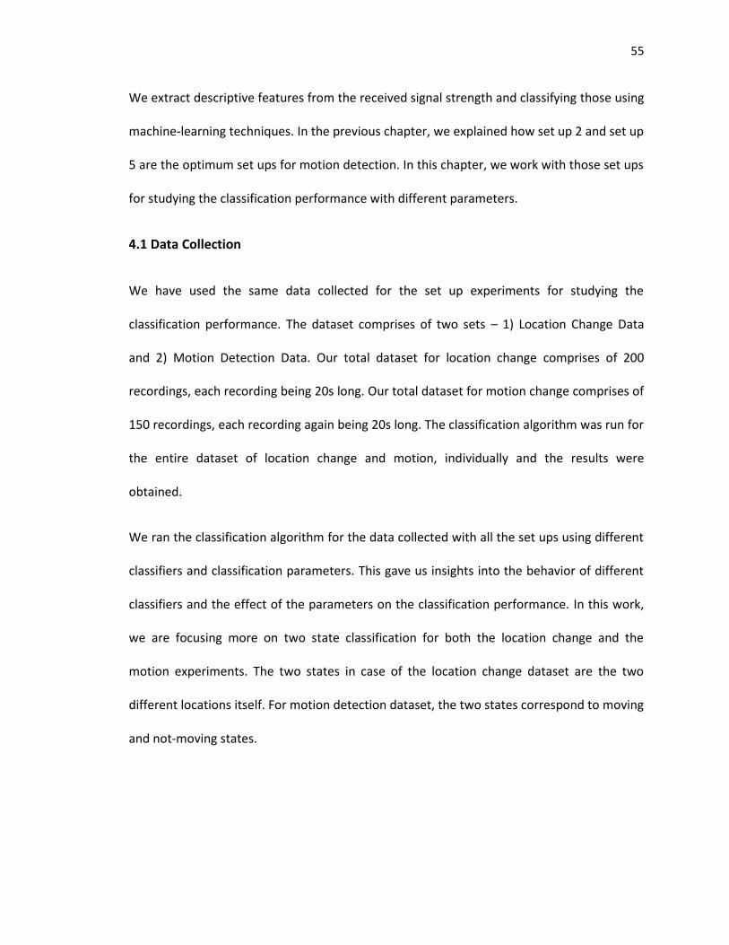
55

We extract descriptive features from the received signal strength and classifying those using

machine-learning techniques. In the previous chapter, we explained how set up 2 and set up

5 are the optimum set ups for motion detection. In this chapter, we work with those set ups

for studying the classification performance with different parameters.

4.1 Data Collection

We have used the same data collected for the set up experiments for studying the

classification performance. The dataset comprises of two sets – 1) Location Change Data

and 2) Motion Detection Data. Our total dataset for location change comprises of 200

recordings, each recording being 20s long. Our total dataset for motion change comprises of

150 recordings, each recording again being 20s long. The classification algorithm was run for

the entire dataset of location change and motion, individually and the results were

obtained.

We ran the classification algorithm for the data collected with all the set ups using different

classifiers and classification parameters. This gave us insights into the behavior of different

classifiers and the effect of the parameters on the classification performance. In this work,

we are focusing more on two state classification for both the location change and the

motion experiments. The two states in case of the location change dataset are the two

different locations itself. For motion detection dataset, the two states correspond to moving

and not-moving states.

56

4.2 Classification Methodology

Our classification approach was to first analyze the RSSI data obtained to study the

distribution pattern under different settings. This helps to determine the best features that

could be used for classification. The classification is a machine learning problem [9, 10] and

we used the WEKA (Waikato Environment for Knowledge Analysis) Classification tool [11] as a

reference for this purpose. We created a feature set and classified the dataset into two

classes with different window lengths and slide lengths. The feature set for location change

experiments consisted of Delta Mean of read rates and Standard Deviation for motion

experiments.

4.2.1 Classification Algorithm

Let X denote the RSSI signal received from a tag:

X =

(5)

where denotes a reading received at the k'th timestamp Tk by antenna Ak .

The mobility status ut at time t (0 <t < tn ), with a classification rule h is given by:

ut = h(X) such that ut = vt (6)

where vt is the actual mobility status of the object at time t. RSSI readings from a distant

time provide little or no information about the mobility at time t. So the input can be

truncated to within a window around t without affecting the performance:

ut = h(X) = h (

) (7)

where w represents the window size. Thus the length of the input signal data to the

function depends upon the window size. The window size in turn also determines the

57

latency involved in the state classification. For example, a window of 3 seconds includes

about 80 RSSI readings.

Once we have the window of data, we extract the sufficient features from that data such as

the standard deviation, delta mean of read rates, etc to form the feature set:

= d (

) (8)

where is the kth feature coefficient at time t. Collectively all these coefficients form the

feature vector. Thus the length of the feature vector is equal to the number of windows

created which in turn depends upon the window size.

In machine learning applications, the classifier has to be first trained using the training set

with pre-assigned labels [9, 10]. The training set used by us is the same data set that is used

for testing. We created a labels vector for the each file and trained the classifier. A label

indicates the state of the object during that interval. The labels file was created with a 1

second interval. For example, consider an experiment Y being conducted which is 20

seconds long and data is collected. Now during Y, the object was still for the first 10 seconds

and was moving for the next 10 seconds. We will label the event stationary as 1 and the

event moving as 2. So the labels file generated for the experiment Y will have 20 values, one

for each second. The first 10 values in the labels file will be 1 and the last 10 values will be 2.

Thus using the pre-defined labels file and the train data set, the classifier trains itself for the

features used.

The problem of estimating the mobility status can now be thought as learning a function g

that maps the feature vector to the mobility status:

ut = g ( ft ) such that ut = vt. (9)

58

In machine learning the function g is known as the classifier, ut a predicted label and vt a

true label.

4.2.2 Classification Parameters

Window Length

Several issues must be considered when choosing the window size. A larger w is useful

under noisy observations as it yields smoother estimates. However, short movements might

be missed with a large w. The latency of the classifier is also proportional to w. The size of

the window and the slide length determines the number of windows generated for that file

which in turn determines the length of the feature set. The average duration of object use is

20 seconds, implying shorter interactions. For detecting such interactions and

generalization, we restricted the window size to 10 seconds.

Slide Length

The slide length is nothing but the amount by which the window slides after each run.

Classifier

We experimented with the following non-temporal classifiers:

1. Support Vector Machines (SVM)

2. Decision Trees (DT)

3. Random Forests (RNF)

The non temporal classifiers were built with the WEKA machine learning toolkit [11].

We also used temporal classification with the Hidden Markov Model (HMM). An HMM is a

generative probabilistic model, which takes the temporal information into consideration.

We built an HMM, where the actual motion states constitute the hidden state set (still or

59

moving) and the estimated states constitute the observation symbols set. Transition

probabilities of the HMM were estimated from the training data. Observations were

modeled as Gaussian mixtures with parameters estimated from the training data based on

the Maximum Likelihood principle.

Features

When an object is standing still, its RSSI pattern may exhibit only slight deviations due to

multipath fading. Changing environmental conditions such as human movement or nearby

tag movement may trigger stronger deviations. However, the most fluctuations observed in

the tag data were during the tag motion itself. For state classification, our aim is to detect

these fluctuations. We have used standard deviation and delta mean as the features to

capture this change. Standard deviation was used for the motion detection experiments and

is a measure of the variation in the signal in the specified window size. Delta mean was used

as a feature for the location change experiments and it represents the amount of change in

average RSSI between two successive windows. Delta mean is supposed to be high when a

location change happens.

4.3 Classification Results

The classification method requires the train and test sets. The train and the test sets were

determined based on the sessions because the readings in a session are correlated. Our

evaluation metric is the classification accuracy. Performance score is determined using the

average classification accuracy over all the sessions in a test set. We performed the

experiments repeatedly with varying window lengths, slide lengths and classifiers to note

the effect of each on the classification accuracy. We have calculated the classification

60

accuracy for all the antenna setups with varying window lengths and slide lengths as well as

different classifiers. The results help us to see the effect of the parameters on the accuracy

and are in correlation with the results from the previous chapter.

We have used three non temporal classifiers namely Decision Tree, Support Vector

Machines, and Random Forest for calculating the accuracies. Non-temporal classifiers are

better in capturing the change in RSSI signal and distinguishing these from environmental

effects.

4.3.1 Location Change Experiments Results

Decision Tree Classification

Figure 4.1: Location Change Classification Accuracy (in percentage): Decision Tree Classifier and varying window

lengths and slide lengths.

0

20

40

60

80

100

120

Set Up 1

Set Up 2

Set Up 3

Set Up 4

Set Up 5

Cla

ssif

icat

ion

Acc

ura

cy

(in

per

cen

tage

)

Location Change Classification Accuracy (in percentage)

WinLen = 3s, Slide Len = 1s

WinLen = 5s, Slide Len= 2s

WinLen = 10s, SlideLen = 10s

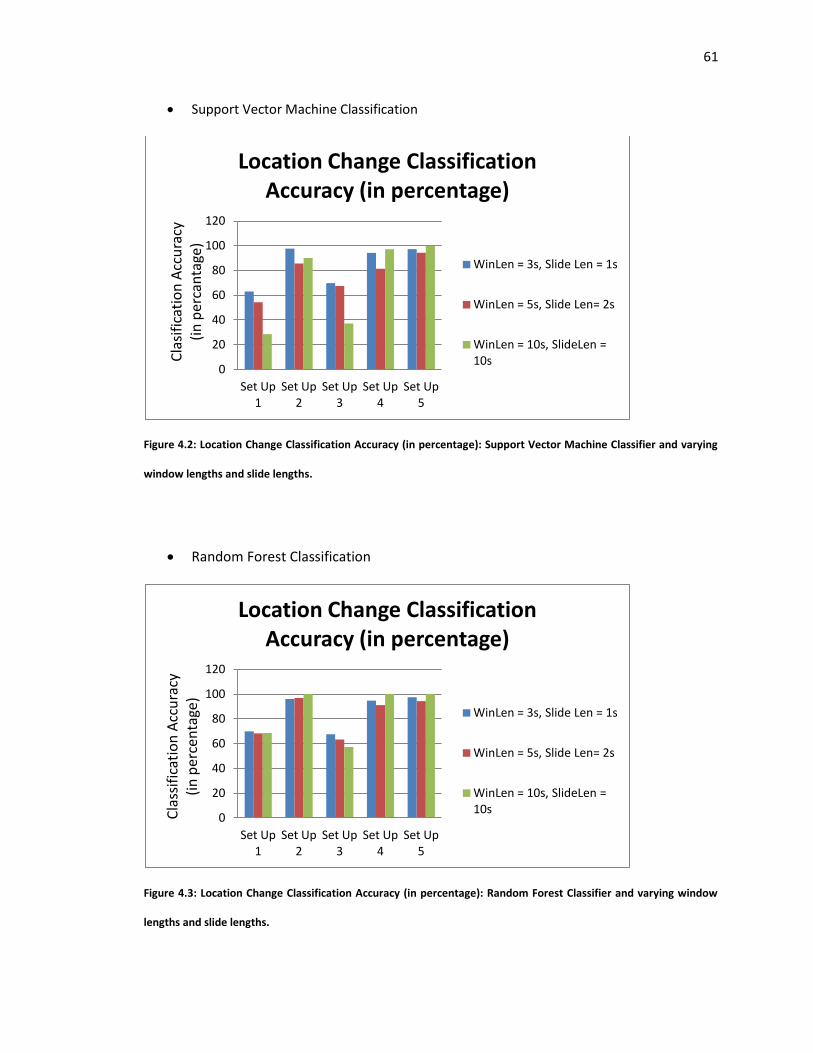
61

Support Vector Machine Classification

Figure 4.2: Location Change Classification Accuracy (in percentage): Support Vector Machine Classifier and varying

window lengths and slide lengths.

Random Forest Classification

Figure 4.3: Location Change Classification Accuracy (in percentage): Random Forest Classifier and varying window

lengths and slide lengths.

0

20

40

60

80

100

120

Set Up 1

Set Up 2

Set Up 3

Set Up 4

Set Up 5

Cla

sifi

cati

on

Acc

ura

cy

(in

per

can

tage

)

Location Change Classification Accuracy (in percentage)

WinLen = 3s, Slide Len = 1s

WinLen = 5s, Slide Len= 2s

WinLen = 10s, SlideLen = 10s

0

20

40

60

80

100

120

Set Up 1

Set Up 2

Set Up 3

Set Up 4

Set Up 5

Cla

ssif

icat

ion

Acc

ura

cy

(in

per

cen

tage

)

Location Change Classification Accuracy (in percentage)

WinLen = 3s, Slide Len = 1s

WinLen = 5s, Slide Len= 2s

WinLen = 10s, SlideLen = 10s

62

4.3.2 Motion Detection Experiments Classification Results

Decision Tree Classifier Results

Figure 4.4: Motion Detection Classification Accuracy (in percentage): Decision Tree Classifier and varying window

lengths and slide lengths.

0

20

40

60

80

100

Set Up 1

Set Up 2

Set Up 3

Set Up 4

Set Up 5

Cla

ssif

icat

ion

Acc

ura

cy

(in

per

cen

tage

) Motion Detection Classification

Accuracy (in percentage)

WinLen = 3s, Slide Len = 1s

WinLen = 5s, Slide Len= 2s

WinLen = 10s, SlideLen = 10s

63

Support Vector Machine Classifier Results

Figure 4.5: Motion Detection Classification Accuracy (in percentage): Support Vector Machine Classifier and varying

window lengths and slide lengths.

Random Forest Classifier Results

Figure 4.6: Motion Detection Classification Accuracy (in percentage): Random Forest Classifier and varying window

lengths and slide lengths.

0

20

40

60

80

100

Set Up 1

Set Up 2

Set Up 3

Set Up 4

Set Up 5

Cla

ssif

icat

ion

Acc

ura

cy

(in

per

cen

tage

)

Motion Detection Classification Accuracy (in percentage)

WinLen = 3s, Slide Len = 1s

WinLen = 5s, Slide Len= 2s

WinLen = 10s, SlideLen = 10s

0

20

40

60

80

100

120

Set Up 1

Set Up 2

Set Up 3

Set Up 4

Set Up 5

Cla

ssfi

cati

on

Acc

ura

cy

(in

per

cen

tage

)

Motion Detection Classification Accuracy (in percentage)

WinLen = 3s, Slide Len = 1s

WinLen = 5s, Slide Len= 2s

WinLen = 10s, SlideLen = 10s

64

As seen from the results above for both location change and motion experiments, set ups 2,

4 and 5 give the best classification accuracies. For location change experiments, the third set

of parameters (window length = 10s and slide length = 10s) yielded the best results. This is

because the experiments were 20s long and the location change happened at the 10th

second. So the two sub-intervals of the first 10s and the next 10s belong to two different

locations and therefore have different RFID signal patters. Thus the results support the

argument that better the separation of the classes, better is the classification accuracy. For

motion experiments, however, smaller window lengths and slide lengths show good results.

A short window yields fewer amounts of data, causing unreliable estimation of features. In

this case, a simple DT can be used.

4.4 Summary

Figure 4.7: Mahalanobis Distance (average) versus Classification Accuracy - All five RFID set ups

0

20

40

60

80

100

120

6.175 12.3625 55.8 88.5 200.845

Mahalanobis Distance versus Classification Accuracy

Mahalanobis Distance versus Classififcation Accuracy

Setup 1 Setup 3 Setup 2 Setup 4 Setup 5

A c c u r a c y (%)

Mahalanobid Distance Values

65

The figure above shows the Mahalanobis distances versus the classification accuracy for all

the setups for location change experiment. Our results show that the distribution distance

values have a correlation with the performance of the RFID set up (as shown in the figure

4.7). More the difference between the distributions of classes, better is the separation

between the classes, more is the classification accuracy. The relationship between the

distribution distance and the classification accuracy is logarithmic rather than being linear.

Setup 2 performs better in terms of classification accuracy because of the presence of two

overhead antennae directly above the zones. The feature set thus formed for setup 2 is

much smaller and classification problem is simplistic. One more important point to note is

that setup 3 has low classification accuracies compared to other setups in spite of having

two overhead antennae. As seen in figure 3.4, setup 3 is a symmetric setup with respect to

the location of the two carts. Hence the RSSI pattern obtained from both the locations is

going to be similar. Hence setup 3 performs badly compared to other setups. Thus, it is

important to create an asymmetric RFID setup as much as possible so that the RSSI patterns

at different locations are not similar.

66

Chapter 5: Conclusion and Future Work

5.1 Conclusion

We have proposed a methodology to evaluate the performance of the RFID systems in a

dynamic work environment. We have closely studied the trauma bay activities and have

proposed five RFID set ups that can be deployed in a trauma bay. We have used the

distribution distance to measure the separation of classes in the RSSI obtained from the

readers.

The results can be used as groundwork for future work on evaluating the RFID systems from

a context aware application point of view. We also conducted experiments for the

placement of tags on objects and studied different scenarios. The tag experiment results

can act as a guideline to be followed for tagging the objects.

We also ran our classification algorithm for all the proposed set ups using different

classifiers and parameters. We have obtained satisfactory results for the classification

accuracy. The results gave us insights into the use of classifiers and parameters to optimize

the performance.

5.2 Future Work

The results obtained in our work are from the data collected in the research lab. We have

also deployed the RFID set up at the Children's National Medical Center, Washington, and

collected real data. The trauma bay was set up with the RFID system and the trauma team

performed a number of activities. The real data can be explored for evaluating the

performance of the RFID set up deployed. The data can be filtered and utilized to evaluate

the RFID setup at the trauma bay in a similar manner as done in chapter 3. Also, the

67

classification algorithm can be run on this data. The results will give interesting insights into

the performance of RFID systems in real world. We have used Mahalanobis distance as a

metric in our work for distribution distance calculation. There are several other distance

metrics like Euclidean distance, Earth Mover's Distance that can be used and the results can

be compared. The feature set used for location change estimation was delta mean whereas

for mobility experiments were standard deviation. Results can be obtained and compared

using other features like combination of both delta mean and standard deviation, mean

RSSI, etc. The application of RFID technology in the trauma bay looks promising and there is

a lot of potential for research in this area.

68

References

1) Steve Hodges, Alan Thorne, Hugo Mallinson, Christian Floerkemeier, "Assesing and Optimizing the Range of UHF RFID to Enable Real World Pervasive Computing Applications" in Pervasive Computing,vol. 4480. Anthony LaMarca,Marc Langheinrich,Khai Truong, Springer Berlin / Heidelberg, 2007, pp 280-297.

2) Lin Wang, Bryan A. Norman, and Jayant Rajgopal, "Placement of Multiple RFID Reader Antennas to Maximize Portal Read Accuracy", International Journal of Radio Frequency Identification Technology and Applications, vol.1,no.3,pp. 260-277,January 2011

3) Matteo Bertocco, Andrea Dalla Chiara, and Alessandro Sona,"Performance Evaluation and Optimization of UHF RFID Systems",Instrumentation and Measurement Technology Conference (I2MTC), 2010, pp. 1175-1180

4) Alien Technology – Products: http:www.alientechnology.com/products/index.php

5) K. Kleisouris, B. Firner, R. Howard, Y. Zhang, and R.P. Martin, “Detecting intra-room mobility with signal strength descriptors,” In Proceedings of the eleventh ACM international symposium on Mobile ad hoc networking and computing, 2010, pp. 71–80

6) Parlak, A. Sarcevic, I. Marsic and R. S. Burd, “Introducing RFID technology in dynamic and time-critical settings: Requirements and challenges” Journal of Biomedical Informatics, 2012.

7) K. M. Ramakrishnan and D. D. Deavours, “Performance benchmarks for passive UHF RFID tags” In Proceedings of the 13th GI/ITG Conference on Measurement, Modeling and Evaluation of Computer and Communication Systems, 2006, pp. 137-154.

8) J. D. Griffin, G. D. Gurgin, A. Haldi and B.Kippelen, “RF tag antenna performance on various materials using radio link budgets,” IEEE Antennas Wireless Propogation Letters, vol. 5, no. 1, pp. 247-250, 2006.

9) E. Alpaydin, “Introduction to Machine Learning”, The MIT Press, 2010. 10) C. Bishop, “Pattern Recognition and Machine Learning”, Springer, 2006.

11) Hall, M., Frank, E., Geoffrey, H., Pfahringer, B., Reuteman, P., Witten, I.H.: The weka data mining software: An update. SIGKDD Explorations 11(1) (2009) 12) Nikitin, P.V. Intermec Technol. Corp., Everett, MA Rao, K.V.S., "Performance Limitations of Passive UHF RFID Systems", Antennas and Propagation Society International Symposium, IEEE, 2006,pp. 1011-1014 13) M. Buettner and D. Wetherall, “An empirical study of UHF RFID performance,” In Proceedings of the 14th ACM international conference on Mobile computing and networking, 2008, pp. 223–234

69

14) D. M. Dobkin, “The RF in RFID: passive UHF RFID in practice,”. Elsevier, 2008. 15) A. Rahmati, L. Zhong, M. Hiltunen and R. Jana, “Reliability techniques for RFID-based object tracking applications,” In Proceedings of IEEE/IFIP International Conference on Dependable systems and Networks, 2007, pp. 113-118. 16) Parlak S, Marsic I, Burd RD. Activity recognition for emergency care using RFID. Proc Int ICST Conf Body Area, Networks;2011 17) Parlak S, Marsic I, Bajwa W, Burd RS. Passive RFID for recognizing activities in trauma care. TRU-IT Technical Report, Rutgers University;November 2011. Available from : http://www.tru-it.rutgers.edu/. 18) Want R. An Introduction to RFID technology. IEEE Pervasive Comput 2006;5(1):25-33 19) Sangwan RS, Qiu RG, Jessen D. Using RFID tags for tracking patients, charts and medical equipment within an integrated health delivery network. Proc IEEE Networking, Sensitivity and Control;2005.p.1070-4 20) Turaga P, Chellapa R, Subrahmanian V, Udrea O. Machine recognition of human activities: a survey. IEEE Trans Circ Syst Video Technol 2008;18(11):1473-88.