Embed Size (px)
Citation preview

EVALUATION OF PERSONNEL PARAMETERS
IN SOFTWARE COST ESTIMATING MODELS
THESIS
Steven L. Quick, Captain, USAF
AFIT/GCA/ENV/03-07
DEPARTMENT OF THE AIR FORCE AIR UNIVERSITY
AIR FORCE INSTITUTE OF TECHNOLOGY
Wright-Patterson Air Force Base, Ohio
APPROVED FOR PUBLIC RELEASE; DISTRIBUTION UNLIMITED.

The views expressed in this thesis are those of the author and do not reflect the official policy or position of the United States Air Force, Department of Defense, or the U. S. Government.

AFIT/GCA/ENV/03-07
EVALUATION OF PERSONNEL PARAMETERS
IN SOFTWARE COST ESTIMATING MODELS
THESIS
Presented to the Faculty
Department of Systems and Engineering Management
Graduate School of Engineering and Management
Air Force Institute of Technology
Air University
Air Education and Training Command
In Partial Fulfillment of the Requirements for the
Degree of Master of Science in Cost Analysis
Steven L. Quick
Captain, USAF
March 2003
APPROVED FOR PUBLIC RELEASE; DISTRIBUTION UNLIMITED.


iv
Acknowledgements
First and foremost, I want to praise my God for giving me the knowledge,
understanding, determination, and supporting family/colleagues/friends needed to
complete this task. I would not have made it without His intervention. To God Be The
Glory.
My family provided continuous support, encouragement, and understanding. I
thank my wife for her unconditional understanding when I needed to spend many long
weeks at school finishing assignments and writing my thesis paper. I know we will be a
better team having gone through it together. My daughter will probably think work is
school since I have been in school thirty-three percent of her life. Thank you for praying
for me and my schoolwork.
I would like to express my sincere appreciation to my thesis advisor, Major Brian
G. Hermann, for his guidance and support throughout the course of this thesis effort.
Your insight and experience were invaluable towards the completion of my research
effort. Your mentorship kept me moving forward when I did not want to proceed nor
knew exactly where I was going.
I would, also, like to thank my sponsor, Major Justin Moul, from the Air Force
Cost Analysis Agency, for both the thesis idea and needed support. You challenged me
beyond my abilities and I am better for it. You also allowed (forced) Captain Charles
Tapp and Lieutenant Tara Case to assist me in obtaining the required technical support
and data to perform the analysis. I cannot imagine working without you.
There are many others that deserve credit for their part in this research. My goal
is to assist others that come after me as I was supported. Thank you all.
Steven L. Quick
v
Table of Contents
Page
Acknowledgements............................................................................................................ iv List of Figures ................................................................................................................... vii List of Tables ..................................................................................................................... ix Abstract ................................................................................................................................x I. Introduction ......................................................................................................................1
General Issue................................................................................................................1 Specific Issue ...............................................................................................................3 Research Objective ......................................................................................................4 Scope of Research........................................................................................................5 Thesis Overview ..........................................................................................................5
II. Literature Review............................................................................................................6
Introduction..................................................................................................................6 Software Cost Estimation ............................................................................................6
Basic process............................................................................................................6 Analogy....................................................................................................................7 Expert opinion..........................................................................................................8 Parametric models....................................................................................................8 State of the practice..................................................................................................9
Risk ............................................................................................................................10 Risk Analysis. ........................................................................................................11 Cost Risk................................................................................................................11 Cost Estimation Risk..............................................................................................12
Software Cost Estimation Models .............................................................................14 COCOMO II. .........................................................................................................14 SEER-SEM. ...........................................................................................................17 SLIM. .....................................................................................................................21 PRICE S. ................................................................................................................25
Design of Experiments (DOE)...................................................................................31 III. Methodology................................................................................................................32
Introduction................................................................................................................32 DOE ...........................................................................................................................32 Research Scenario......................................................................................................34

vi
Page
Data Collection ..........................................................................................................35 COCOMO II. .........................................................................................................35 SEER-SEM. ...........................................................................................................38 SLIM. .....................................................................................................................39 PRICE S. ................................................................................................................40
Data Analysis .............................................................................................................41 IV. Results..........................................................................................................................43
Chapter Overview ......................................................................................................43 Individual Model Results ...........................................................................................43
COCOMO II. .........................................................................................................43 SEER-SEM. ...........................................................................................................52 SLIM. .....................................................................................................................57 PRICE S. ................................................................................................................64
Model Comparisons ...................................................................................................71 Overall Personnel Parameter Impact Comparison .....................................................72
V. Conclusion ....................................................................................................................74
Overview....................................................................................................................74 Results........................................................................................................................75 Future Research .........................................................................................................81
Appendix 1 COSTAR VBA code ......................................................................................82 Appendix 2 COSTAR Commands.txt file .........................................................................84 Appendix 3 Modified COSTAR VBA code ......................................................................89 Appendix 4 SEER-SEM VBA Code..................................................................................93 Appendix 5 SLIM VBA Code ...........................................................................................97 Appendix 6 PRICE S APPL Values ..................................................................................99 Appendix 7 COSTAR Data Table ...................................................................................102 Appendix 8 SEER-SEM Data Table................................................................................119 Appendix 9 SLIM Data Table..........................................................................................130 Appendix 10 PRICE S Data Table...................................................................................141 Bibliography ....................................................................................................................142

vii
List of Figures
Page
Figure 1. Increased Software Dependency [6:55] ...........................................................................................2
Figure 2. Software Cost Estimation Accuracy versus Program Phase [12:311]..............................................3
Figure 3. COCOMO II Effort Estimate Inputs ..............................................................................................15
Figure 4. SEER-SEM Parameter's Relative Impact [24:Ch7, 18] .................................................................19
Figure 5. SLIM Project Environment Input Screen [25:22] ..........................................................................22
Figure 6. SLIM Solution Assumptions Input Screen [25:24] ........................................................................23
Figure 7. SLIM Default PI Calculator [25:102] ............................................................................................24
Figure 8. SLIM PI Detail: Personnel Profile [25:104]..................................................................................24
Figure 9. PRICE S Equation Relationships [26:167] ...................................................................................25
Figure 10. Productivity Factor Table, PROFAC [26:168].............................................................................26
Figure 11. Price Software Volume [26:169]..................................................................................................27
Figure 12. Price S Application Mix Generator Form [26:123]......................................................................27
Figure 13. Software Volume vs. Labors Hours [26:171]...............................................................................28
Figure 14. CPLX1 Labor Hour Impact Graph [26:184] ................................................................................29
Figure 15. CPLXM Labor Hour Impact Graph [26:188]...............................................................................30
Figure 16. Software Cost Estimation Process [29:19]...................................................................................31
Figure 17. COCOMO II Effort Multiplier Groups ........................................................................................32
Figure 18. Costar Modified Excel file "Data" worksheet ..............................................................................37
Figure 19. COCOMO II Personnel Effort Multipliers Spider Plot ................................................................47
Figure 20. COCOMO II Personnel Parameters Productivity Range .............................................................48
Figure 21. Overall COCOMO II Personnel Parameters Impact ....................................................................49
Figure 22. COCOMO II Personnel Effort Multiplier Distribution ................................................................50
Figure 23. COCOMO II Calculated Personnel Effort Impact ......................................................................51
Figure 24. SEER-SEM Personnel Parameters Spider Plot ............................................................................54
Figure 25. SEER-SEM Personnel Parameters Productivity Range ...............................................................54

viii
Page
Figure 26. Overall SEER-SEM Personnel Parameters Impact ......................................................................55
Figure 27. SEER-SEM Personnel Effort Multiplier Data Distribution .........................................................56
Figure 28. Overall SEER-SEM Calculated Personnel Effort Impact ............................................................57
Figure 29. SLIM Personnel Parameters Spider Plot ......................................................................................59
Figure 30. SLIM Personnel Parameters Productivity Range .........................................................................60
Figure 31. Overall SLIM Personnel Parameters Impact................................................................................61
Figure 32. SLIM Personnel Effort Multipliers Data Distribution..................................................................62
Figure 33. Overall Calculated SLIM Personnel Effort Impact ......................................................................63
Figure 34. PRICE S CPLX1 Actual Impact [26:185]....................................................................................65
Figure 35. PRICE S CPLXM Actual Effort Impact [26:188]........................................................................66
Figure 36. PRICE S Productivity Range .......................................................................................................66
Figure 37. PRICE S Personnel Parameters Spider Plot .................................................................................67
Figure 38. PRICE S PROFAC Effort Estimate Impact .................................................................................68
Figure 39. PRICE S Overall Personnel Effort Impact Results ......................................................................69
Figure 40. PRICE S Personnel Effort Multiplier Distribution.......................................................................70
Figure 41. Overall PRICE S Personnel Effort Impact ...................................................................................70
Figure 42. Parametric Model Personnel Comparison....................................................................................71
Figure 43. Parametric Model Personnel Parameter Impact Comparison.......................................................73
Figure 44. COSTAR Excel file......................................................................................................................82

ix
List of Tables
Page
Table 1. COCOMO II Personnel Factors [23:47-49] ...................................................................................15
Table 2. Model Personnel Parameters ...........................................................................................................34
Table 3. Experiment Software Development Scenario.................................................................................35
Table 4. Costar Initial Inputs .........................................................................................................................36
Table 5. SEER-SEM Initial Inputs ................................................................................................................39
Table 6. SLIM Model Initial Inputs...............................................................................................................39
Table 7. PRICE S Initial Inputs .....................................................................................................................40
Table 8. COSTAR Trials For Multiplier Calculation ....................................................................................45
Table 9. COCOMO II Personnel Parameters Effort Multipliers ...................................................................45
Table 10. COCOMO II Effort Multiplier Independence Test ......................................................................46
Table 11. COCOMO II Post-Architecture Group Productivity Ranges ........................................................49
Table 12. SEER-SEM Calculated Effort Multipliers.....................................................................................52
Table 13. SEER-SEM Effort Multiplier Independence Test .........................................................................53
Table 14. SLIM Calculated Effort Multipliers ..............................................................................................58
Table 15. SLIM Effort Multiplier Independence Test ...................................................................................59
Table 16. PRICE S Calculated Effort Multipliers .........................................................................................64
Table 17. PRICE S Effort Multiplier Independence Test ..............................................................................65

x
AFIT/GCA/ENV/03-07
Abstract
Software capabilities have steadily increased over the last half century. The
Department of Defense has seized this increased capability and used it to advance the
warfighter’s weapon systems. However, this dependence on software capabilities has
come with enormous cost. The risks of software development must be understood to
develop an accurate cost estimate.
Department of Defense cost estimators traditionally depend on parametric models
to develop an estimate for a software development project. Many commercial parametric
software cost estimating models exist such as COCOMO II, SEER-SEM, SLIM, and
PRICE S. COCOMO II is the only model that has open architecture. The open
architecture allows the estimator to fully understand the impact each parameter has on the
effort estimate in contrast with the closed architecture models that mask the quantitative
value with a qualitative input to characterize the impact of the parameter.
Research was performed to determine the quantitative impact of personnel
parameters on the effort estimate in the closed architecture models. Using a design of
experiments structure, personnel parameters were varied through three levels for each
model. The data was then analyzed to determine the impact of each parameter at each
level by evaluating the change from a baseline estimate. The parameters were evaluated
to determine characteristics including linearity, independence between input parameters,
impact range and effort multipliers. The results will enable DoD cost estimators to
understand potential estimation errors resulting from inaccurately assessing each input
factor. Risk ranges can be built around the final estimate based on the research results.

1
EVALUATION OF PERSONNEL PARAMETERS
IN SOFTWARE COST ESTIMATING MODELS
I. Introduction
General Issue
“Software spending in the Department of Defense (DoD) and NASA is
significant, and it continues to increase” [1, 6-1]. The United States government and
business sectors spent $70 billion in 1985 [2] on software development compared to $230
billion in 2000 [3]. In 1992 DoD spent approximately $24 billion to $32 billion on
software requirements. “Estimates also indicate that total annual software costs could
increase to about $50 billion in the next 15 years, accounting for almost 20 percent of
Defense’s [DoD’s] overall budget” [4:2]. DoD spending increases are due, in part, to a
greater dependence on software to improve the warfighting capabilities of the warfighter.
According to the former Deputy Under Secretary of Defense (Science and Technology),
Dr. Delores Etter, “Software is pervasive. It truly is the new physical infrastructure. We
are more dependent on software than ever, and software is becoming more complex”
[5:3]. In this era of near continuous software capabilities expansion and defense force
structure downsizing, software programs and instructions are relied upon to maintain our
defense capabilities. Figure 1 shows this increasing software dependence in terms of the
percent of functions performed by software in selected DoD weapon systems [6:54].

2
WeaponSystem Year
F-4 1960A-7 1964
F-111 1970F-15 1975F-16 1982B-2 1990F-22 2000
Percent of FunctionsPerformed in Software
810
80
20354565
Figure 1. Increased Software Dependency [6:55]
Amid this increasing dependence, the need for increased management of software
development costs was brought to center stage during the development of the McDonnell
Douglas transport aircraft designated the C-17. In 1985, at the beginning of
development, the estimated lines of code (LOC) needed for all C-17 software systems
was 164,000. The actual figure would grow over the next five years of development to
1,356,000 LOC, making the C-17 “the most computerized, software-intensive, transport
aircraft ever built” [7:2]. By May 1992, the program was estimated to be “2 years behind
schedule and $1.5 billion over the 1985 program cost estimate of $4.1 billion” [7:14].
Pentagon officials became so concerned that in 1993 one of the program managers was
fired, three other Air Force officials were given reduced punishment, and the program
was targeted for cancellation [8].
This increased dependence on software highlights software development as a
major cost driver in new weapon system development programs. Therefore, accurate
software development cost estimates are essential to the Air Force for use in out-year
budget formulation to ensure funds are available to pay for approved programs. The
estimation problem is even more widespread as “27 percent of software development
projects come in on time and on budget…” [9:13].

3
However, according to Ferens [10], DoD software cost analysts do not have
adequate information about their software development projects to construct accurate
software cost estimates. Boehm points out that cost estimate accuracy increases the closer
the project gets to completion (Figure 2). In later stages of a software project, more
accurate measures of estimation parameters, such as code size and personnel
productivity, are available. Thus, the software effort and cost estimate ranges are reduced
over time [11].
Figure 2. Software Cost Estimation Accuracy versus Program Phase [12:311]
Specific Issue
Software cost estimates are developed by different methods such as commercial
parametric models, analogy, expert opinion, and bottom-up. The estimate could also be a

4
combination of one or more these methods. Each estimation technique has its own
strengths and weaknesses. In general, all techniques build the cost estimate by
developing a cost estimating relationship between project independent parameters (e.g.,
size, domain, etc) and dependent cost estimation values (e.g., effort, cost, and schedule).
Parametric models, the most widely used DoD technique to estimate software
cost, relate multiple independent parameters with dependent variables via mathematical
formulae. The mathematical formulae are developed using statistical procedures and a
historical database of software project costs. Most parametric models in use today are
proprietary. Thus, the mathematical formulae are not published for analysts to study and
gain an understanding of how cost estimates are generated.
Cost analysts who utilize these proprietary parametric programs to construct a
software cost estimate and who do not have some statistical educational background, do
not understand the relative effects each parameter has on the cost estimate. However, this
information is desirable to account for the uncertainty associated with the input parameter
values. With this understanding, estimators could provide a more realistic cost estimate
range rather than a misleading and frequently inaccurate point estimate.
Research Objective
The objective of this study is to determine the relative change of a cost estimate
from a baseline estimate as parameter input values are altered from the lowest rating to
the highest rating and size is held constant. The secondary objective is to use the results
of the experiment to develop risk factors that will enable analysts to develop cost estimate
ranges based on the uncertainty and impact of the subject parameter values.

5
Scope of Research
The Air Force Cost Analysis Agency has requested that this research utilize the
following commonly used parametric models: COCOMO II, SEER-SEM, SLIM, and
PRICE S. Personnel parameters will be the only parameters that will be adjusted. Other
parameters will be set at the nominal setting. The size parameter will be set to 40,000
source lines of code.
Thesis Overview
Chapter II, Literature Review, summarizes the most current techniques used to
incorporate risk into the cost estimate. Each parametric model will be reviewed for
similarities and differences.
Chapter III outlines the methodology, Design of Experiments (DOE), to evaluate
the selected parameters’ effect on the cost estimate. Additionally, the process for
calculating the calibration factors is explained.
Chapter IV, Findings and Analysis, presents the results of the DOE. These results
are used to develop the risk factors.
Chapter V, Conclusions and Recommendations for Follow-up Research, explains
whether or not the objectives were met. Recommendations for further research are given.

6
II. Literature Review
Introduction
This chapter summarizes the recent research on the software cost estimation
process, cost estimation methods, and the current state of cost estimation. It covers
parametric models that will be utilized to evaluate the impact of cost parameters other
than size and identifies which model parameters to use in the design of experiment
(DOE). The DOE procedures are described in the methodology chapter. The scope of
the review is limited to the four parametric software cost estimation models: SEER-SEM,
COCOMO II, SLIM, and PRICE S.
Software Cost Estimation
The Society of Cost Estimation and Analysis defines cost estimating as “the art of
approximating the probable cost or value of something, based on information available at
the time” [13: n. pag.]. Thus, software cost estimation is the process of approximating
the cost of producing a software product. The process can have different designs
depending on the type of software under development, but each process has the same
basic structure.
Basic process.
The basic process of estimating software cost is 1) determine what work/effort
must be performed at some productivity level; and 2) over what time to produce the
software product. Effort is then expensed at some dollar rate to obtain the cost of the

7
product. Lawrence Putnam uses a simple generic mathematical formula to illustrate this
relationship between product, effort, productivity, and time (see Eq. 1).
Product = Productivity * Effort * Time (1)
where Product = size of software (e.g., source lines of code (SLOC) or function
points)
Productivity = “a measure of the amount of product produced per unit of human effort” [14:36]; measured in SLOC/manmonth
Effort = manmonths or manyears Time = months or years [14:26-36]. The variables of the equation must be determined to solve for effort. The effort would
then be multiplied by the budgeted labor rate to get the estimated cost. The estimator can
employ a number of methods to produce the equation values: 1) analogy, 2) expert
opinion, and 3) parametric models (15).
Analogy.
The analogy method uses information from previous projects. An analyst who
uses this method knows that the new project is similar to the completed project(s). Final
costs of projects with similar components or requirements, adjusted for design or
complexity changes, would be used to develop the cost estimate for the new project.
Detailed technical data is a requirement to ensure the analogous system is truly similar if
this method is used (15). This method will not be used in the research effort since
parametric model parameters are the focus.

8
Expert opinion.
Expert judgment techniques rely on data from one or more experts. Estimators
must ensure that anyone asked to provide information has adequate knowledge and
experience with the past projects and the new requirements to provide meaning
information. For example, in the Delphi method experts are sent a questionnaire to
answer. After the responses are returned to the originator, all the feedback is sent back
out to the respondents. Responses are kept anonymous. Then the process is repeated.
The estimate is refined as the iterations are completed until a final estimate is agreed on.
The main point is to eliminate bias within the group setting. Expert opinion is not
encouraged, however, due to inconsistency in the accuracy of individual estimates [1].
Therefore, expert opinion will not be considered in this research.
Parametric models.
Parametric models are the focus of this thesis. Parametric models are
mathematical equations that have one or more inputs to generate the output. The inputs
and outputs have been statistically proven to have independent/dependent correlations.
That is to say the inputs, such as complexity or programmer capability, are the
independent factors and outputs, such as cost or effort, are the dependent parameters.
Software projects have many different computer software configuration items
(CSCIs) that make up the final software product. Each one of the CSCIs has an
individual cost estimate that makes up the final project cost estimate. Parametric models
have the benefit of speed because only a few inputs are needed based on the
mathematical equation. Another advantage is the accuracy of the estimate. Parametric

9
estimates are as accurate as those estimates from other models, provided the models have
been calibrated and validated. DoD prefers the parametric models given these benefits
[1].
However, just using a parametric model does not guarantee accuracy. One study
shows that the correct setting of the individual parameters is more important than using
the correct model [16]. Four of the parametric models widely used by DoD personnel are
Constructive Cost Model (COCOMO), Galorath Software Evaluation and Estimation of
Resources Software Estimating Model (SEER-SEM®), Software Life-Cycle Model
(SLIM), and Price Software Model (PRICE S®). These models’ equations and input
parameters will be described later in this chapter.
State of the practice.
The history of software cost estimation began with the software era in the 1940s.
Cost estimation was performed manually with simple relationships and equations
developed by individual companies. The need for improved software cost estimation
grew as the software engineering field developed. Air Force, Army, Hughes Aircraft,
IBM, RCA, and TRW funded research to learn what factors where driving software
development costs [17].
Many parametric models were developed from the early research such as PRICE
S, SLIM, COCOMO, SEER-SEM, and CHECKPOINT. As of 1998, there were at least
50 different models to choose from [17]. Over time many of the models have developed
similar input parameters. Size has always been the dominating parameter, but other
parameters include “program attributes such as domain, complexity, language, reuse, and
required reliability; choices of computer attributes such as time and storage constraints

10
and platform volatility; choices of personnel attributes such as capability, continuity, and
experience; and choices of project attributes such as tools and techniques, requirements
volatility, schedule constraints, process maturity, team cohesion, and multisite
development” [18:940].
Although the models have had many improvements and estimation features
added, the accuracy of the model estimates are still questionable. Ferens reports on
numerous studies performed for the DoD using many of the commercial software
estimating models that 25 percent accuracy is the best that can be anticipated half of the
time. The accuracy did not improve even after calibrating to a military data set. Ferens
contends that DoD cost analysts cannot be expected to have accurate estimates since
parametric models are more often than not the method utilized [10]. The study of risk
analysis must be considered to understand why accurate cost estimates are important.
Risk
Nicholas states, “Every project is risky, meaning there is a chance things won’t
turn out exactly as planned. Project outcomes are determined by many things, some that
are unpredictable and over which project managers have little control” [19:306]. These
risks normally cause the cost of the project to increase. Air Force budget managers
develop out-year budgets based on forecasted project expenditures. The forecasted
project expenditures are developed based on the project cost estimate. Therefore, it is
imperative that the project cost estimate capture a reasonable amount of the potential cost
that the risks impose, because not including the risk costs would leave the project under
funded should one of the risks occur.
11
Risk Analysis.
“Risk analysis is the quantifying, either qualitatively or quantitatively, of the
probability and the potential impact of some risk” [20:1]. Risk analysis includes the
following steps: “risk identification, risk assessment, and risk response planning”
[19:307]. The project has to be broken down into manageable units before the risk
analysis can be performed.
There are two ways to divide a project into component parts, process or product
structure. In the case of an aircraft, the process structure would divide the project into the
overarching phases such as requirements, design, development, test & evaluation,
manufacturing, and operational support. Similarly, the product structure could be cockpit
section, propulsion section, fuselage section, wings section, and tail section. These
would be further divided unto the lowest division of work. The end result of either
method is a Work Breakdown Structure (WBS).
The risks of completing each item can be determined systematically using the
WBS. The risks are assessed for project impact and probability of occurrence to
determine which risks should be focused on. Developing a plan to manage the risks is
the last step in risk analysis; however, the risk assessment should be reevaluated
periodically and used to develop the cost estimate.
Cost Risk.
Cost estimation, if performed correctly, includes the information obtained from
the risk analysis. The initial cost estimate is developed by using the WBS and estimating
how much each part will cost. This initial estimate is normally referred to as a point

12
estimate since it does not include the effects of risk. Cost risk is the cost impact if the
risk event occurs. Coleman calls this “the funds set aside to cover predicted cost growth”
where cost growth is the “increase in cost of a system from inception to completion”
[21:4].
The point estimate is modified by including the risk analysis data for each WBS
element. When the risk assessment is performed, possible outcomes are evaluated based
on the impact to technical requirements, schedule, and cost and the probability of each
outcome occurring. The cost ranges developed from the risk assessment along with the
corresponding probabilities are incorporated into the estimate. Using Monte Carlo
simulation techniques a range of cost estimates are generated with corresponding
probability of occurrence [21]. (It should be noted that this process is more complicated
than addressed here. It is not the intent of this paper to explain how the estimation
process should be performed, but how it is linked with the risk analysis.)
Cost Estimation Risk.
Cost Estimating Risk is “risk due to cost estimating errors, and the statistical
uncertainty in the estimate” [21:5]. The cost analyst uses the WBS to develop the project
estimate. Project engineers or WBS element experts can be interviewed to determine the
cost range and probabilities of occurrence. Historical data might also provide another
source of information on the cost of a project. The risk exits that the analyst will make a
mistake in determining the appropriate cost data to use in developing the estimate using
either approach.
Software cost analyst depend mainly on commercial off-the-shelf (COTS) cost
estimating tools such as COCOMO II, SEER-SEM, SLIM, and PRICE S. The analyst

13
needs very little data to be able to develop an initial estimate. Estimated size,
complexity, development environment complexity, and personnel capabilities are some
of the data needed to populate the estimating tool.
How the models input parameters affect the final estimate is important to
understand to be able to develop proper risk adjusted estimates due to the dependence on
COTS models. The Clinger Cohen Act requires a risk adjusted estimate for all
information system projects [22]. The focus of this research is to determine the impact of
three of the most frequently used COTS models to provide a foundation for risk ranges.

14
Software Cost Estimation Models
These model descriptions will only cover the development cost estimation process
since the research is focused on the development costs.
COCOMO II.
Barry Boehm, a pioneer in software cost estimation, first started working on the
COCOMO model in the 1970s as an engineer for TRW. This model has become the
most widely used parametric model to date. The popularity is due to it being an open
model since Boehm published all the equations, parameter level coefficients, and
development details in his famous book Software Engineering Economics, in 1981 [12].
The current version, COCOMO II, was released in 2000. This version updates the
database to 161 projects used to develop the parameter coefficients, adds some new effort
multiplier parameters, and allows function point sizing. Three models are used to
generate an estimate for the full life of the product: early prototyping phase, early design
phase, and post-architecture phase [23]. This thesis will focus on the post-architecture
model.
The post-architecture model is used when the product is ready for full scale
development. Therefore, much of the needed detail, such as requirements and design, to
characterize the product and construct an estimate are readily available. The formula
used to calculate the effort in person-months is
∏=
××=n
ii
E EMSizeAPM1
(2)
where A = 2.94 EMi = each effort multiplier not rated at nominal
∑=
×+=5
101.0
jjSFBE

15
where B = 0.91 SFj = each scale factor value
The three main inputs are effort multipliers (EMs), scale factors, and size. Size and scale
factors will not be discussed since this research is holding the size parameter constant.
Figure 3 shows the different factors that go into the COCOMO II effort estimate [23].
Figure 3. COCOMO II Effort Estimate Inputs
The effort multipliers are categorized into four groups: Personnel factors, Product
factors, Platform factors, and Project factors. COCOMO’s effort multipliers are used to
explain the productivity of the development team which directly impacts the effort
needed for the project. “After product size, personnel factors have the strongest influence
in determining the amount of effort required to develop a software product” [23:47]. The
impact of each effort multiplier is quantitatively expressed in Table 1. The value for
analyst capability at the very low (VL) rating means the effort required will be 42% more
than the base effort estimate when set at nominal (N). No other model openly explains
all equations and model input relationships to this detail.
Table 1. COCOMO II Personnel Factors [23:47-49]
Personnel Factors VL L N H VH Productivity
Range Analyst Capability 1.42 1.19 1.00 0.85 0.71 2.00 Programmer Capability 1.34 1.15 1.00 0.88 0.76 1.76 Personnel Continuity 1.29 1.12 1.00 0.90 0.81 1.51 Applications Experience 1.22 1.10 1.00 0.88 0.81 1.51 Platform Experience 1.19 1.09 1.00 0.91 0.85 1.40 Language and Tool Experience 1.20 1.09 1.00 0.91 0.84 1.43
Effort (Person Months)
Effort Multipliers Scale Factors Size (SLOC or FP)
Other

16
COCOMO’s personnel factors are used to explain the ability and know-how of
the development team as opposed to an individual on the team. Analysts that are rated
high (H) will not expend as much effort to get requirements and design finished as
compared to analysts that are rated low (L). Programmer capability is concerned with the
“ability, efficiency and thoroughness, and the ability to communicate and cooperate” of
the programmers as a team [23:47]. Personnel continuity evaluates the annual personnel
turnover expected during the project. Applications experience rates the development
team’s experience with the application under development. For example, a low rating
would be given if the team had less than two month’s experience. Platform experience
explains the team’s knowledge of platforms like graphic user interface or networking.
Language and tool experience takes into account the software development tools to be
used on the project [23].

17
SEER-SEM.
“SEER-SEM is a tool for software estimation, planning and project control.
SEER-SEM estimates software development and maintenance effort, cost, schedule,
staffing, reliability, and risk” [24:Ch2,2]. This section describes the input parameters and
equations used to generate the estimate outputs.
SEER-SEM utilizes knowledge bases to develop the initial estimate. “A
knowledge base is a set of parameter values, based on actual project, requirement, and
environmental data similar to your estimating scenario, which can be used to initialize
parameter values in your WBS [work breakdown structure] elements” [24:Ch6,1]. The
user selects the appropriate knowledge bases and inputs the size estimate, which gives the
model enough information to calculate an estimate. All parameter values will be set to
the nominal value if knowledge bases are not chosen when the project is created. The
following is a list of the seven knowledge bases and their definitions:
1. Platform - explains where the software will be utilized, like aircraft, space or ships [24].
2. Application – explains the general use of the software; “Examples
include: artificial intelligence (AI), computer aided design (CAD), command and control, communications, database, diagnostics, financial, flight, graphics, management information systems (MIS), mission planning, operating system/executive, process control, radar, robotics, simulation, and utilities” [24:Ch2,7].
3. Acquisition Method – explains how the software will be acquired,
such as all new code, modification, rehosting, and others or some combination.
4. Development Method – “Describes the methods to be used during
development, such as rapid application development (RAD), traditional waterfall, object-oriented, prototype, spiral, or incremental” [24:Ch2,7].
18
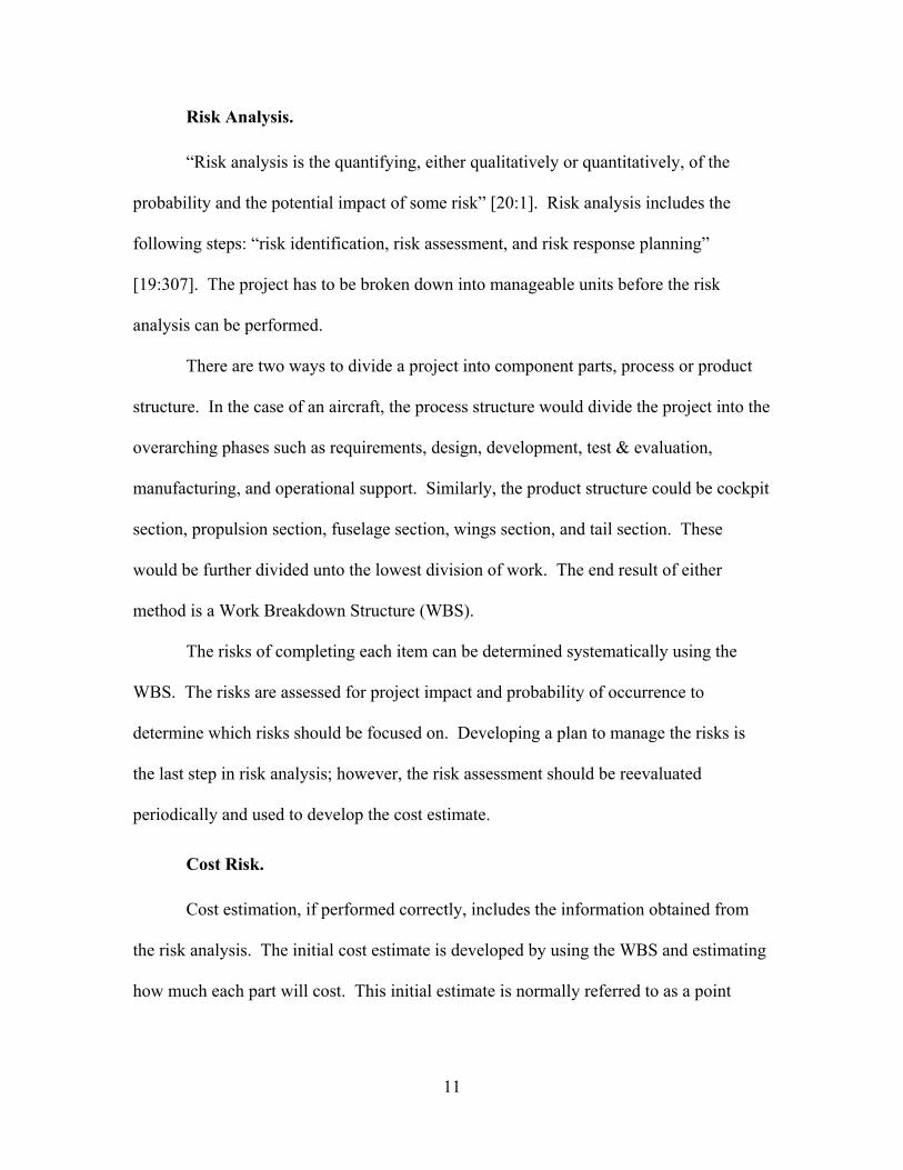
5. Development Standard – “Describes the documentation, reliability, and test standards to be followed such as ISO, IEEE, ANSI, military, informal, or none at all” [24:Ch2,7].
6. User Defined – “Describes special user-defined classifications of
software” [24:Ch2,7]. 7. Component Type – “(COTS only) Describes those parameters that
are relevant to particular types of commercial software packages” [24:Ch2,7].
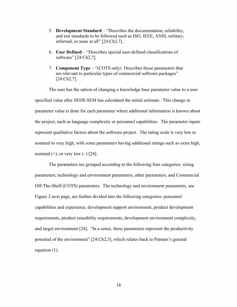
The user has the option of changing a knowledge base parameter value to a user
specified value after SEER-SEM has calculated the initial estimate. This change in
parameter value is done for each parameter where additional information is known about
the project, such as language complexity or personnel capabilities. The parameter inputs
represent qualitative factors about the software project. The rating scale is very low to
nominal to very high, with some parameters having additional ratings such as extra high,
nominal (+), or very low (–) [24].
The parameters are grouped according to the following four categories: sizing
parameters, technology and environment parameters, other parameters, and Commercial
Off-The-Shelf (COTS) parameters. The technology and environment parameters, see
Figure 2 next page, are further divided into the following categories: personnel
capabilities and experience, development support environment, product development
requirements, product reusability requirements, development environment complexity,
and target environment [24]. “In a sense, these parameters represent the productivity
potential of the environment” [24:Ch2,3], which relates back to Putnam’s general
equation (1).

19
Figure 4 is a graph depicting the relative impact on cost and effort. Security
requirements are shown to have the highest impact, while target system complexity has
the smallest impact. The actual parameter impact values are not given.
0% 20% 40% 60% 80% 100% 120% 140% 160% 180% 200%
Security Requirements
Target System Volatility
Target System Complexity
Real Time Code
Time Constraints
Memory Constraints
Special Display Requirements
TARGET ENVIRONMENT
Process Improvement
Application Class Complexity
Host Development System Complexity
Language Type (complexity)
DEVELOPMENT ENVIRONMENT COMPLEXITY
Software Impacted by Reuse
Reusability Level Required
PRODUCT REUSABILITY REQUIREMENTS
Rehost from Development to Target
Quality Assurance Level
Test Level
Specification Level - Reliability
Requirements Volatility (Change)
PRODUCT DEVELOPMENT REQUIREMENTS
Process Volatility
Host System Volatility
Resource and Support Location
Resource Dedication
Multiple Site Development
Terminal Response Time
Logon thru Hardcopy Turnaround
Automated Tools Use
Modern Development Practices
DEVELOPMENT SUPPORT ENVIRONMENT
Practices & Methods Experience
Target System Experience
Host System Experience
Programmer's Language Experience
Programmer Capabilities
Analyst's Application Experience
Analyst Capabilities
PERSONNEL CAPABILITIES & EXPERIENCE
Parameters' relative impact on cost and effort
399%
Figure 4. SEER-SEM Parameter's Relative Impact [24:Ch7, 18]
The mathematical equations and how they work will be explained in general
terms since SEER-SEM is a proprietary model. SEER-SEM uses the following software
equation:

20
tCS dtee K= (3)
where Se = effective size (input) Cte = effective technology (input) K = effort (output) td = schedule (output)
Size is input by the user. SEER-SEM calculates the effective technology constant from
the qualitative parameter settings. The complexity equation (4) is required to solve for
effort and schedule since there are still two unknown variables:
3dtKD = (4)
where D = staffing complexity (input)
Staffing complexity is calculated by SEER-SEM from the user inputs. The software
equation is solved for td (5) and substituted (6) into the complexity equation (4).
KCS
tte
ed = (5) 3
=
KCS
KD
te
e
(6)
Effort (K) is the only unknown equation (6),. Therefore, effort can be solved:
2.14.0
=
te
e
CS
DK (7)
Schedule can be calculated by replacing effort in the software equation with equation (7)
now that one unknown is solved. Schedule would equal
4.02.0
= −
te
ed C
SDt (8)
21
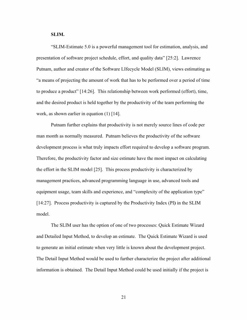
SLIM.
“SLIM-Estimate 5.0 is a powerful management tool for estimation, analysis, and
presentation of software project schedule, effort, and quality data” [25:2]. Lawrence
Putnam, author and creator of the Software LIfecycle Model (SLIM), views estimating as
“a means of projecting the amount of work that has to be performed over a period of time
to produce a product” [14:26]. This relationship between work performed (effort), time,
and the desired product is held together by the productivity of the team performing the
work, as shown earlier in equation (1) [14].
Putnam further explains that productivity is not merely source lines of code per
man month as normally measured. Putnam believes the productivity of the software
development process is what truly impacts effort required to develop a software program.
Therefore, the productivity factor and size estimate have the most impact on calculating
the effort in the SLIM model [25]. This process productivity is characterized by
management practices, advanced programming language in use, advanced tools and
equipment usage, team skills and experience, and “complexity of the application type”
[14:27]. Process productivity is captured by the Productivity Index (PI) in the SLIM
model.
The SLIM user has the option of one of two processes: Quick Estimate Wizard
and Detailed Input Method, to develop an estimate. The Quick Estimate Wizard is used
to generate an initial estimate when very little is known about the development project.
The Detail Input Method would be used to further characterize the project after additional
information is obtained. The Detail Input Method could be used initially if the project is

22
far enough along in the development cycle. Project Environment and Solution
Assumptions are the main input areas need to develop the initial estimate.
The Project Environment screen Project Description tab, Figure 5, allows
development characteristics to be input such as Application Type and Application Type
mix. SLIM uses Application Type and Application Type % to calculate the default PI
available to the project. SLIM has nine application types: Microcode, Real Time,
Avionic, System Software, Command & Control, Telecommunications, Scientific,
Process Control, and Business. The remaining tabs on this screen have default settings
that do not need inputs for an initial estimate.
Figure 5. SLIM Project Environment Input Screen [25:22]
Solution Assumption inputs are the next required data, Figure 6. These inputs
include Basic Info, Phase Tuning, and Accounting. The Basic Info tab allows the user to
input start date, phases to include in the estimate, staffing buildup, estimated size of the

23
project, and PI. Many of the fields are pre-filled with SLIM defaults. The minimum
inputs needed to generate an estimate are the start date, size information, and PI.
Figure 6. SLIM Solution Assumptions Input Screen [25:24]
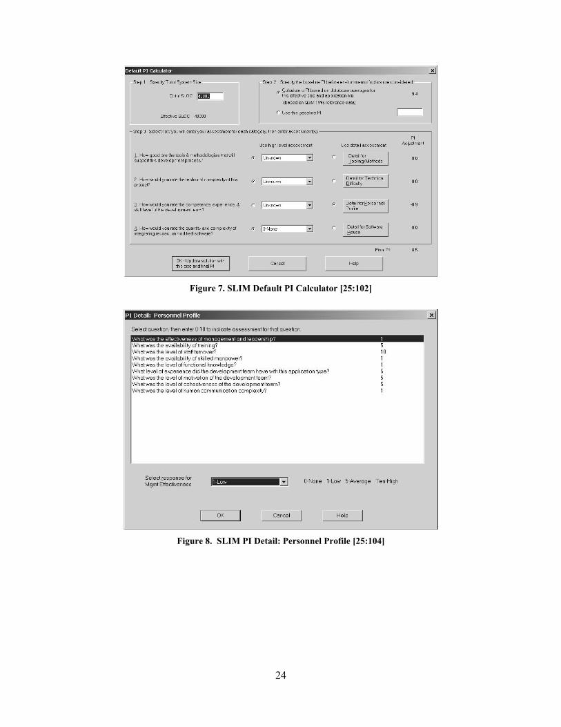
The default PI, based on the size estimate and development complexity, is
calculated using a historical database of over 5,000 projects. The development
complexity that impacts the PI is divided into three areas: tooling and methods, technical
difficulty, and personnel factors. These areas can be rated at an aggregate or detail level
as shown in Figure 7, default PI Calculator and Figure 8, PI Detail. The rating scale is
from 0 to 10 with 5 being an average score. These complicating factors each have an
equal impact on the PI.
24
Figure 7. SLIM Default PI Calculator [25:102]
Figure 8. SLIM PI Detail: Personnel Profile [25:104]

25
PRICE S.
The PRICE S model calculates cost and schedules for software development
projects. Even though the model has parametric equations, the company takes pride in
the fact that the model does not depend strictly on statistical relationships to develop an
effort estimate. The model was developed to allow the analyst to use valuable experience
when characterizing the development team. PRICE S does not rely on one parametric
equation or single data base. Instead, inputs capture aspects of the software development
process that affects effort [26].
The model was first built with regression analysis and then enhanced to allow the
analyst to include experience based opinion that tailors the model to the analyst’s
company. Effectively creating different equations for each project as the analyst
calibrates the model. Figure 9 is a representation of the PRICE S model parameter
relationships. Productivity (PROFAC), Volume, and Complexity (APPL) make up the
core equation. Complicating factors are then introduced to determine the additional
effort required to complete the development [26].
Figure 9. PRICE S Equation Relationships [26:167]
$ Estimate
Phase/Function Allocations
Labor Rates
Overhead
Inflation
Cost of Money
G&A
Profit
Overtime
Tools
Timing/Memory Constraints
Schedule Constraints
Schedule Lengths
Schedule Overlaps
Personnel Skill Level
Internal/External Interfaces
No. of Locations
Reengineering/Reuse
Compl’d Effort
Spec Level
Technology Maturity
Volumne
Complexity
Productivity

26
“PROFAC is an empirically derived parameter that includes such items as skill
levels, experience, productivity, and efficiency” [26:119]. This value is determined by
PRICE S using completed projects of the company or PRICE S industry standard values,
Figure 10. Type of platform under development is determined first if PRICE S values are
to be used.
Platform “is a measure of the transportability, reliability, testing, and
documentation which must be provided for acceptable contract performance” [26:18].
Platform categories are Commercial Proprietary Software, Commercial Production
Software, Military Software, and Space Software with values ranging from 0.6 to 2.5
respectively [26].
Next, the PROFAC values are associated with each Platform value as shown in
Figure 6. Each grouping has a high, nominal, and low setting. For example, airborne
military software platform value is 1.8. Therefore, the PROFAC range would be 5.5 to
6.5. The PROFAC would be 5.0 if the organization’s personnel experience was nominal
[26].
Figure 10. Productivity Factor Table, PROFAC [26:168]

27
The software volume value of the project under development is the product of
size, a function value of language type, and APPL, Figure 11. Price Systems uses
Volume to describe the total amount of work that must be completed. Size can be input
as source lines of code, function points, or predictive object points. APPL describes the
complexity of the software under development based on what functions the actual code
will be performing.
Figure 11. Price Software Volume [26:169]
The APPL value is entered using the APPL Generator, Figure 12. The value can be
entered by the user based on experience or historical data or calculated by PRICE S based
on a percent of each
Figure 12. Price S Application Mix Generator Form [26:123]
Complexity
Size Unit
Language

28
type of functionality in the development such as 20 percent Online Communication, 10
percent Math, etc where the sum must equal 100 percent. Price Systems provides a table
of APPL values, Appendix 6, which can be used to choose an APPL value for many
different types of applications since some of the code functionality is not listed in the
APPL generator.
PRICE S uses a core equation to calculate the labor hours (LH) required to
complete the development if no other complicating factors were introduced now that
Productivity, Volume, and Complexity have been determined. The core equation
[26:171] is
( )[ ]1000
PROFACfPROFAC VOLeLH ∗= (9)
Figure 13 shows the relationship software volume has to labor hours at different levels of
organizational productivity. It is intuitive that the more software functions to produce or
volume required more effort is needed. The graph also indicates that the more productive
the personnel are less effort will be required to complete the task.
Figure 13. Software Volume vs. Labors Hours [26:171]
29
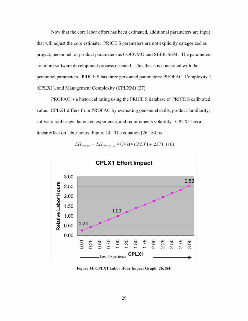
Now that the core labor effort has been estimated, additional parameters are input
that will adjust the core estimate. PRICE S parameters are not explicitly categorized as
project, personnel, or product parameters as COCOMO and SEER-SEM. The parameters
are more software development process oriented. This thesis is concerned with the
personnel parameters. PRICE S has three personnel parameters: PROFAC, Complexity 1
(CPLX1), and Management Complexity (CPLXM) [27].
PROFAC is a historical rating using the PRICE S database or PRICE S calibrated
value. CPLX1 differs from PROFAC by evaluating personnel skills, product familiarity,
software tool usage, language experience, and requirements volatility. CPLX1 has a
linear effect on labor hours, Figure 14. The equation [26:184] is
( ) ( )237.1763.111 +∗∗= = CPLXLHLH CPLXCPLX (10)
CPLX1 Effort Impact
0.24
1.00
2.53
0.00
0.50
1.00
1.50
2.00
2.50
3.00
0.01
0.25
0.50
0.75
1.00
1.25
1.50
1.75
2.00
2.25
2.50
2.75
3.00
CPLX1
Rel
ativ
e La
bor H
ours
Figure 14. CPLX1 Labor Hour Impact Graph [26:184]
Less Experience

30
“CPLXM is used in PRICE S to model the effects of management complications,
such as multiple development locations or multinational projects, on the cost of a
software development” [26:187]. The more complex the management scenario the more
effort required to ensure communication is maintained between the customer and the
development staff. Figure 15 shows the linear impact of CPLXM on the effort estimate.
The labor hour equation [26:188] for CPLXM is
( ) ( )683.3172.1 +∗∗= = CPLXMLHLH CPLXMCPLXM (11)
CPLXM Effort Impact
1.00
1.32
1.63
0.90
1.00
1.10
1.20
1.30
1.40
1.50
1.60
1.70
0.01 0.25 0.50 0.75 1.00 1.25 1.50 1.75 2.00 2.25 2.50 2.75 3.00
CPLXM
Rel
ativ
e La
bor H
ours
Figure 15. CPLXM Labor Hour Impact Graph [26:188]

31
Design of Experiments (DOE)
The research methodology used to gather data is Design of Experiments (DOE).
DOE is a scientific method that systematically allows the researcher to collect unbiased
data about a process under study. “A designed experiment is a test or series of tests in
which purposeful changes are made to the input variables of a process or system so that
we may observe and identify the reasons for changes in the output response” [28:1]. This
research will involve six factors at three different levels for a total of 729 data points.
Thus, a factorial design will be developed to account for all possible combinations of
factors and levels used in the process.
The process in this research is software cost estimation, Figure 16, using
parametric models. Some of the inputs to the process are product requirements,
personnel factors, product size, and development environment complexity. The output
variable is effort in man months. It is important for the cost estimator to know the impact
that each input variable has on the output variable to be able to correctly characterize the
development team and produce an accurate estimate. Additionally, when estimates are
verified by a different parametric model, knowing how the input affects the effort output
will allow the estimator to evaluate the differences in the two estimates.
Figure 16. Software Cost Estimation Process [29:19]

32
III. Methodology
Introduction
The objective of this study is to determine the relative change of a cost estimate
from the baseline estimate as the personnel parameter input values are altered from the
lowest rating to the highest rating while size and other parameters are held constant. The
secondary objective is to use the results of the experiment to develop risk factors that will
enable analysts to develop cost estimate ranges based on the uncertainty and impact of
the subject parameter values. Design of Experiments (DOE) will be used to collect
COCOMO II, SEER-SEM, SLIM, and PRICE S effort data for analysis. The data will be
analyzed for change in effort, generalization of parameter effects, range of impact, and
linear or non-linear impact.
DOE
COCOMO II has 17 effort multipliers in the Post-Architecture model. The effort
multipliers are categorized into four groups as shown in Figure 17. Collecting all the
possible combinations between all 17 factors at the lowest and highest setting would take
131,072 trials. The trials would increase to 129,140,163 with three settings. Therefore,
the number of factors in the experiment will be limited to an acceptable amount of trials.
Figure 17. COCOMO II Effort Multiplier Groups
Effort Multipliers
Product Factors Platform Factors Personnel Factors Project Factors

33
Boehm reports that personnel factors have the greatest impact on estimated effort
after size [23]. The SLIM model documentation also indicates that productivity factors
have the most impact on calculating the effort after size [25]. SLIM’s productivity factor
subsumes nine different personnel parameters. Therefore, this research will concentrate
on the personnel inputs from each of the four models.
The COCOMO II model uses six parameters to characterize the personnel
influences. These parameters at three different settings will generate 729 different
possible combinations. With the exception of PRICE S, each of the models has at least
six personnel parameters. Some of the personnel factors, Table 2, will have to be
eliminated from the research to enhance cross model validation and arrive at a
manageable trial size. The personnel parameters from SEER-SEM and SLIM will be
compared to the other models. Any parameter not in one of the other models will be
excluded from the research. The parameters not included will be SEER-SEM, Practices
& Methods Experience; and Questions 2, 7, and 8 in SLIM. Personnel parameters not
included in the research will be set to their nominal values.

34
Table 2. Model Personnel Parameters
COCOMO II SEER-SEM Analyst Capability Analyst Capabilities Programmer Capability Analyst's Application Experience Personnel Continuity Programmer Capabilities Applications Experience Programmer's Language Experience Platform Experience Host System Experience Language and Tool Experience Target System Experience
Practices & Methods Experience
SLIM Question 1: How good is management and leadership on this project (0-10)? Question 2: What is the availability of training (0-10)? Question 3: What is the anticipated level of staff turnover (0-10)? Question 4: What is the availability of skilled manpower (0-10)? Question 5: What is the level of functional knowledge (0-10)? Question 6: How experienced is the development team with this application type (0-10)? Question 7: How motivated is the development team (0-10)? Question 8: How cohesive is the development team (0-10)? Question 9: What is the level of human communication complexity (0-10)?
PRICE-S
Productivity Factor Complexity (Personnel Skills/Tools) Management Complexity
Research Scenario
The experiment was conducted using an unmanned space development scenario.
The software to be developed will be for a single CSCI. Code will be written to control a
signal processing unit. The code will be 100 percent new developed code eliminating the
complexity of reuse code in the estimate equation. The language utilized will be Ada 95.
The quality standard imposed on the development project will be ANSI J-STD-016 Nom.
Estimated size of this software development will be 40,000 SLOC. This scenario, Table
3, will be used to provide the models with initial inputs. Model parameters not using this
information will be set to the nominal setting.

35
Table 3. Experiment Software Development Scenario
Unmanned Space Signal Processing New Development Ada 95 ANSI J-STD-016 Nom Size – 40,000 SLOC Waterfall design
Data Collection
The data will consist of 729 individual runs, a full 36 factorial design for each
model except PRICE S. PRICE S data will consist of 27 data points, a full 33 factorial
design. A fractional factorial design will not be performed because the capability to
batch process three of the models exists. SLIM data will be collected manually since it
does not have batch processing capability. The batch processing is performed using
Excel and Visual Basic for Applications (VBA). However, each model’s process is
different and will be explained. The VBA coding will not be explained in detail, but is
provided in the appendix section.
COCOMO II.
The COCOMO II software cost estimation software provided with Boehm’s book,
Software Cost Estimation With COCOMO II, does not have batch processing capability.
However, Softstar Systems offers a software program that does have batching capability
which can be calibrated to 13 different COCOMO models which included COCOMO II.
Therefore, the COCOMO II data will be collected using the Softstar Systems software
called Costar, version 6.05. The Costar initial input settings are provided in Table 4.

36
Table 4. Costar Initial Inputs
COSTAR Model Type COCOMO II 2000 Phases Waterfall Size 40,000 SLOC Effort Unit Man Months Scale Factors
Precedentedness Somewhat unprecedented Development Flexibility Some Relaxation Architecture/Risk Resolution Often 60% Team Cohesion Basically Cooperative Process Maturity SEI CMM Level 2
Effort Multipliers Post-Architecture
Softstar Systems provides an Excel VBA file, Appendix 1, and Costar commands
text file, Appendix 2, that allows the user to change the setting of one parameter at a time.
To use the Excel file, the Costar VBA code will be modified to allow multiple parameter
changes. The modified VBA code is located in Appendix 3. This code allows six
parameters to be changed through 3 different settings and record each runs development
effort estimate into the Excel file “Experiment” worksheet.
Module one will create the DOE matrix of all 729 trials in the Costar required
format and command text. The parameter command names and command setting levels
are first entered into the “Data” worksheet as shown in Figure 18. The levels can be
entered in as numeric values or alpha command codes. Once the parameters and levels
are entered, the macro CreateCostarExperimentMatrix is run. Module one will create the
matrix in the “Experiment” worksheet. Module 2, docostar subroutine, is automatically
started after Module one is executed.

37
Figure 18. Costar Modified Excel file "Data" worksheet
Module two uses the array table of parameters and settings on the “Data”
worksheet, Figure 18, to write a “Costar.cmd” file which interfaces with the Costar
software. The command file generates a Costar report file of the effort estimate. The
original Costar VBA code is written to collect the total project effort estimate. Total
project effort estimate is located on line 17 of the generated report. Line 17 is referenced
in the VBA code as follows:
' Read Costar results ' Open tempdir + "costar.out" For Input As #1 For i = 1 To 17 Input #1, mystring Next i

38
This code will be modified to capture only development costs by changing the 17 to 15.
This tells the VBA code to read the 15th line on the report instead of the 17th line.
Module 2 will collect all 729 runs one after the other.
SEER-SEM.
“SEER-SEM has the capability to execute a stream of commands, either from the
clipboard or a text file” [24:15-7]. This capability is called Server Mode by SEER-SEM.
The clipboard procedures will be utilized for this research. Procedures can be found in
the 2000 user’s manual page 15-8 and Appendix B. Also, the SEER-SEM software
provides an Excel file1 which has instructions, sample script, and required command text
for running the Server Mode option.
Clipboard option works by first developing the command strings. The command
strings are then copied to the clipboard. The estimate can then be determined by running
the command string through SEER-SEM by selecting from the main menu “File” then
“Execute Clipboard”.
The command string is developed using VBA code located in Appendix 4,
module 1. The Excel file must contain two worksheets named “Data” and “Experiment”
to create the command string. “Data” worksheet is where the parameter names and
setting values required by Server Mode are entered. The VBA code then creates the
command string for 729 different runs, names the text export file where the effort
estimate data will be saved, and names the project file for future reference. Module 2
will be used to format the experiment matrix and copy the command string to the
1 C:\SEER\SEM6-0\SEER-SEM Server Mode Details V6.0e.xls

39
clipboard. The effort estimate data has to be retrieved manually from the text export file
to be analyzed. Table 5 provides the initial inputs to SEER-SEM.
Table 5. SEER-SEM Initial Inputs
SEER-SEM Platform Knowledge Base !No Knowledge Application Knowledge Base !No Knowledge Acquisition Method Knowledge Base !No Knowledge Development Method Knowledge Base !No Knowledge Development Standard Knowledge Base !No Knowledge Size 40,000 SLOC
SLIM.
The SLIM model does not have the capability to batch process each different
parameter combination. Therefore, the data will be collected by inputting the initial
settings, Table 6, for
Table 6. SLIM Model Initial Inputs
SLIM Effort Unit Man Month Application Type Realtime Industry Sector Military Product Construction
Function Unit SLOC Radio Button Selection Integrated Gearing Factor 1
Application Type % Realtime: 100% Predominant Development Machine Workstation Predominant Operating System Other Default PI Calculator
Step 1 40,000 Step 2 Calculate a PI Step 3
1. Tools & Methodology Unknown 2. Technical Complexity Unknown 3. Personnel Profile Detail for Personnel Profile 4. Reuse None
Schedule and Cost Equal
40
the baseline scenario. Then the SLIM experiment matrix will be followed changing one
parameter setting at a time and recording the effort estimate for analysis. The VBA code
used to create the experiment matrix is located in Appendix 5.
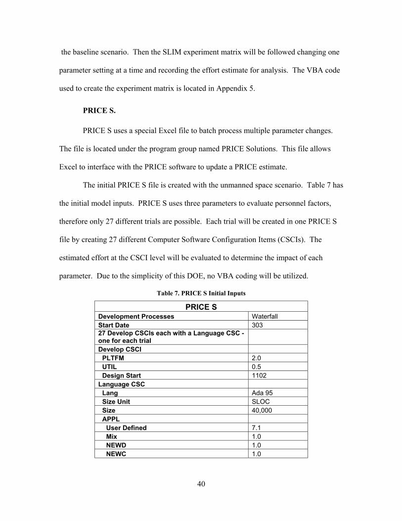
PRICE S.
PRICE S uses a special Excel file to batch process multiple parameter changes.
The file is located under the program group named PRICE Solutions. This file allows
Excel to interface with the PRICE software to update a PRICE estimate.
The initial PRICE S file is created with the unmanned space scenario. Table 7 has
the initial model inputs. PRICE S uses three parameters to evaluate personnel factors,
therefore only 27 different trials are possible. Each trial will be created in one PRICE S
file by creating 27 different Computer Software Configuration Items (CSCIs). The
estimated effort at the CSCI level will be evaluated to determine the impact of each
parameter. Due to the simplicity of this DOE, no VBA coding will be utilized.
Table 7. PRICE S Initial Inputs
PRICE S Development Processes Waterfall Start Date 303 27 Develop CSCIs each with a Language CSC - one for each trial Develop CSCI
PLTFM 2.0 UTIL 0.5 Design Start 1102
Language CSC Lang Ada 95 Size Unit SLOC Size 40,000 APPL
User Defined 7.1 Mix 1.0 NEWD 1.0 NEWC 1.0

41
Data Analysis
The data for each model will be analyzed separately to determine the impact each
parameter has on the effort estimate at the lowest and highest setting. The nominal effort
estimate will be the initial baseline. The following formula will be used to determine the
change from nominal:
−+=
Nom
Nomn
XXX
Multiplier 1 (12)
where Xn is Effort estimate of the nth trial
XNom is Effort estimate where all personnel parameters are set at the nominal setting (baseline estimate)
Effort multipliers are determined for each parameter setting by locating each trial that has
all the levels set at nominal save one after the impact of each combination of parameter
settings is calculated. For example, to find the multiplier for Analyst Capability at the
lowest skill setting in the COCOMO II trials, the trial run settings would be ACAP, 1.42;
all other parameters would be set to the nominal value of one. The effort multiplier will
be a fixed value if the model uses linear multiplication in the effort estimate equation to
account for the parameter impact on the effort estimate.
Boehm used linear multiplication in the COCOMO estimation equation. The
effort multipliers used in COCOMO are fixed for the given qualitative settings. This
assumption that multipliers do not change is grounded in Boehm’s belief that the impact
of each cost driver is independent of the other cost drivers. Linear interpolation can be
implemented to derive a value between the published values given this independence
[23].

42
Independence between the cost drivers will be determined by changing the
baseline effort estimate (XNOM) used to calculate the initial multipliers. The new baseline
will be the first cost driver used from each model, set at the highest skill level, while the
rest of the cost drivers are set to the nominal value. For example, the original XNOM for
the COCOMO II data is the effort estimate from COSTAR trial 356, all cost drivers set to
the nominal value. The new XNOM used for the independence test will be COSTAR trial
608. For each parameter, independence will be shown if the new effort multipliers do not
change from the original effort multipliers given the new baseline. This test will allow
the multiplier to be generalized beyond the cost scenario developed to collect the current
data.
Range impact of each parameter will be determined after the multiplier is
calculated. The range information will provide the cost analyst the knowledge of which
personnel parameter has the most impact to effort. The analyst’s main focus should be
placed on the accurate estimates for parameters that impact effort the greatest. Also,
effective risk ranges could be developed based on the parameter impact values should the
analyst not be able to obtain an adequate parameter estimate to include in the cost
estimate model.
The last item to check for is linear or nonlinear effects of the personnel
parameters as a whole. Three levels were included in the research to determine linearity.
Linearity or nonlinearity will be determined by graphing the effort multipliers at the
different skill levels.
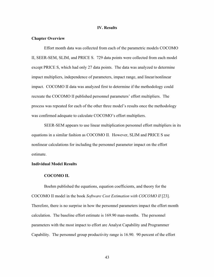
43
IV. Results
Chapter Overview
Effort month data was collected from each of the parametric models COCOMO
II, SEER-SEM, SLIM, and PRICE S. 729 data points were collected from each model
except PRICE S, which had only 27 data points. The data was analyzed to determine
impact multipliers, independence of parameters, impact range, and linear/nonlinear
impact. COCOMO II data was analyzed first to determine if the methodology could
recreate the COCOMO II published personnel parameters’ effort multipliers. The
process was repeated for each of the other three model’s results once the methodology
was confirmed adequate to calculate COCOMO’s effort multipliers.
SEER-SEM appears to use linear multiplication personnel effort multipliers in its
equations in a similar fashion as COCOMO II. However, SLIM and PRICE S use
nonlinear calculations for including the personnel parameter impact on the effort
estimate.
Individual Model Results
COCOMO II.
Boehm published the equations, equation coefficients, and theory for the
COCOMO II model in the book Software Cost Estimation with COCOMO II [23].
Therefore, there is no surprise in how the personnel parameters impact the effort month
calculation. The baseline effort estimate is 169.90 man-months. The personnel
parameters with the most impact to effort are Analyst Capability and Programmer
Capability. The personnel group productivity range is 16.90. 90 percent of the effort

44
multipliers fell between 0.45 and 2.26. The effort multipliers can be used as risk factors
as suggested by Boehm [23]. The raw COCOMO II data from each trial is located in
Appendix 7.
Effort Multipliers.
COCOMO II uses effort multipliers to characterize how cost drivers will impact
the development effort. The post-architecture model is used to calculate the estimate for
the development and maintenance stage of the software project. The product of the effort
multipliers is multiplied by the nominal effort estimate to calculate the project effort
estimate. The nominal effort estimate is calculated with all effort multipliers set to
nominal rating, a value of 1.00. Linear interpolation between effort multiplier values is
acceptable for the majority of the multipliers [23].
The nominal development effort estimate generated from the initial inputs from
Table 3 is 169.90 person-months. The effort multiplier for each trial was calculated using
the formula
−+=
Nom
Nomn
XXX
Multiplier 1 (12)
where Xn is effort months of the nth trial and XNom is nominal effort months. The effort for each cost driver at the three different levels was determined by
locating the trials where all the parameter values were set to the nominal rating except the
parameter level to be determined. For example, trial 608 was used to determine the
multiplier value for Analyst Capability at the highest skill level. Table 8 shows each trial
used to determine the multiplier values for each level. The same sequence of trials was
used to analyze each of the other models’ data. The calculated multiplier values were the

45
Table 8. COSTAR Trials For Multiplier Calculation
Run ACAP PCAP PCON APEX PLEX LTEX Effort Months Multiplier
Costar 122 1.42 1 1 1 1 1 241.20 1.42 Costar 284 1 1.34 1 1 1 1 227.60 1.34 Costar 338 1 1 1.29 1 1 1 219.10 1.29 Costar 356 1 1 1 1.22 1 1 207.20 1.22 Costar 362 1 1 1 1 1.19 1 202.20 1.19 Costar 364 1 1 1 1 1 1.2 203.90 1.20 Costar 365 1 1 1 1 1 1 169.90 1.00 Costar 366 1 1 1 1 1 0.84 142.70 0.84 Costar 368 1 1 1 1 0.85 1 144.40 0.85 Costar 374 1 1 1 0.81 1 1 137.60 0.81 Costar 392 1 1 0.81 1 1 1 137.60 0.81 Costar 446 1 0.76 1 1 1 1 129.10 0.76 Costar 608 0.71 1 1 1 1 1 120.60 0.71
same as the COCOMO II published personnel effort multipliers, Table 9. Therefore, the
multiplier formula explains the impact of each level if the effort estimation model
formula uses a linear multiplier to capture the parameter impact.
Table 9. COCOMO II Personnel Parameters Effort Multipliers
Driver Lowest Nominal Highest Analyst Capability (ACAP) 1.42 1.00 0.71
Programmer Capability (PCAP) 1.34 1.00 0.76 Personnel Continuity (PCON) 1.29 1.00 0.81
Applications Experience (APEX) 1.22 1.00 0.81 Platform Experience (PLEX) 1.19 1.00 0.85
Language/Tool Experience (LTEX) 1.20 1.00 0.84
Generalization of Multipliers – Independence Test.
The COCOMO II published effort multipliers were replicated using the data
collection process and multiplier formula. The effort multiplier formula used the nominal
effort estimate as the baseline, indicating the parameters are not impacting the effort
estimate, to calculate the multiplier values. The parameters are said to be independent if
the change in the effort estimate can be explained by each parameter’s impact
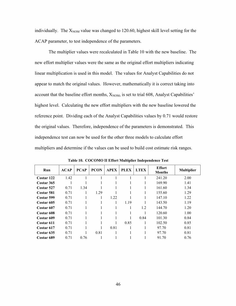
46
individually. The XNOM value was changed to 120.60, highest skill level setting for the
ACAP parameter, to test independence of the parameters.
The multiplier values were recalculated in Table 10 with the new baseline. The
new effort multiplier values were the same as the original effort multipliers indicating
linear multiplication is used in this model. The values for Analyst Capabilities do not
appear to match the original values. However, mathematically it is correct taking into
account that the baseline effort months, XNOM, is set to trial 608, Analyst Capabilities’
highest level. Calculating the new effort multipliers with the new baseline lowered the
reference point. Dividing each of the Analyst Capabilities values by 0.71 would restore
the original values. Therefore, independence of the parameters is demonstrated. This
independence test can now be used for the other three models to calculate effort
multipliers and determine if the values can be used to build cost estimate risk ranges.
Table 10. COCOMO II Effort Multiplier Independence Test
Run ACAP PCAP PCON APEX PLEX LTEX Effort Months Multiplier
Costar 122 1.42 1 1 1 1 1 241.20 2.00 Costar 365 1 1 1 1 1 1 169.90 1.41 Costar 527 0.71 1.34 1 1 1 1 161.60 1.34 Costar 581 0.71 1 1.29 1 1 1 155.60 1.29 Costar 599 0.71 1 1 1.22 1 1 147.10 1.22 Costar 605 0.71 1 1 1 1.19 1 143.50 1.19 Costar 607 0.71 1 1 1 1 1.2 144.70 1.20 Costar 608 0.71 1 1 1 1 1 120.60 1.00 Costar 609 0.71 1 1 1 1 0.84 101.30 0.84 Costar 611 0.71 1 1 1 0.85 1 102.50 0.85 Costar 617 0.71 1 1 0.81 1 1 97.70 0.81 Costar 635 0.71 1 0.81 1 1 1 97.70 0.81 Costar 689 0.71 0.76 1 1 1 1 91.70 0.76

47
Impact Range.
The impact each parameter will have on the effort estimate is graphically seen in
Figure 19. The slope of the line from lowest to nominal is steeper than the slope from
nominal to highest. This indicates that an improvement in skill level between the lowest
and nominal rating will reduce effort more dramatically that further improves from
nominal to highest. The rest of the skill level data points are necessary for a complete
characterization.
Impact of Individual Personnel Parameters
0.600.700.800.901.001.101.201.301.401.50
Lowest Nominal HighestSkill Level
Effo
rt Mu
ltiplie
r Analyst CapabilityProgrammer CapabiliyPersonnel ContinuityApplications ExperiencePlatform ExperienceLanguage/Tool Experience
Figure 19. COCOMO II Personnel Effort Multipliers Spider Plot
The values of each parameter at the lowest and highest levels are used to calculate
the individual productivity range and determine which parameter has the most impact on
effort. The individual productivity range measures the overall impact of each parameter.
This value is calculated by dividing the largest multiplier value by the smallest multiplier
value. The productivity range for Analyst Capability is 2.00, 1.42 divided by 0.71.
Analyst Capability impacts the effort estimate more than any of the other personnel
parameters as seen in Figure 20.

48
Productivity Range
2.00
1.59
1.51
1.40
1.76
1.43
0.00 0.50 1.00 1.50 2.00 2.50
Analyst Capability (ACAP)
Programmer Capabiliy (PCAP)
Personnel Continuity (PCON)
Applications Experience (APEX)
Platform Experience (PLEX)
Language/Tool Experience (LTEX)
Figure 20. COCOMO II Personnel Parameters Productivity Range
The fact that Analyst Capabilities impacts the effort estimate the most makes
sense from a software development stand point. Analysts determine the initial
requirements and software design which typically takes more effort than coding. The
programmers use the initial design and requirements to complete the coding process.
Tremendous effort would be wasted if the initial design must be reaccomplished due to
incorrect analysis.
Boehm calculates the individual productivity range for all the COCOMO II effort
multipliers in the front cover of his book [23]. The book shows the Analyst Capability
parameter has the second most impact on the effort estimate of the 17 parameters. The
individual productivity range is the first level to evaluate effort impact. The next level is
the group productivity range.
The group productivity range is the product of the individual productivity ranges.
This definition is consistent with how Boehm’s states that the personnel parameters have
the most impact on the effort estimate since the personnel group productivity range is
largest of the four cost driver groupings [23]. The productivity range for each cost driver

49
group is shown in Table 11. This indicates that more resources should be spent on
determining the personnel and product parameter ratings since their impact can be much
greater than platform and project parameters’ impact.
Table 11. COCOMO II Post-Architecture Group Productivity Ranges
Cost Driver Group Productivity Range Product Parameters 10.40 Platform Parameters 3.56 Personnel Parameters 16.90
Project Parameters 3.27
The impact of the personnel parameters on effort can be seen in Figure 21. This
graph shows the effort estimate for all 729 different trials used in the experiment verses
the corresponding effort multiplier. The highest skill level combination resulted in an
effort estimate that was 25 percent of the nominal estimate. The lowest skill level
increased the effort estimate to 428 percent of the nominal estimate.
COCOMO II Experiment Results
0.25, 42.90
4.28, 726.40
0.00
100.00
200.00
300.00
400.00
500.00
600.00
700.00
800.00
0.00 0.50 1.00 1.50 2.00 2.50 3.00 3.50 4.00 4.50
Effort Multiplier
Effo
rt (M
an M
onth
s)
1.00, 169.90
Figure 21. Overall COCOMO II Personnel Parameters Impact

50
The effort months were distributed from a low of 42.90 to a high of 726.40
person-months and corresponding effort multipliers from 0.25 to 4.28 respectively.
Using Palisade Decision Tools’ Best Fit 4.5 software, the best fit distribution for the
effort multipliers was the Gamma distribution using the Chi-Square for Goodness-of-fit,
Figure 22.
The graph shows that 90 percent of the effort multiplier combination values are
between 0.45 and 2.26. 47 percent of the values are below the nominal value of 1.00.
The 90 percent interval could be used to develop a risk range if the personnel parameters
could not be determined. Notice that this distribution does not imply the likelihood of the
personnel parameter being estimated at one value when they are in fact actually another.
That data comes from estimates of completed projects which is not collected by the DoD.
Gamma(2.5749, 0.35911) Shift=+0.23066
0.0
0.2
0.4
0.6
0.8
1.0
0.0
0.5
1.0
1.5
2.0
2.5
3.0
3.5
4.0
4.5
>5.0%90.0%0.449 2.260
BestFit Student VersionFor Academic Use Only
Figure 22. COCOMO II Personnel Effort Multiplier Distribution

51
Linear/Nonlinear Impact.
The personnel parameters appear to have an exponential effect on the effort
estimate as seen in Figure 23. The effort estimate increases significantly as the skill level
moves from a nominal rating to a low rating. The change from nominal to the highest
skill level rating has a smaller slope indicating that the increase in skill level does not
impact the effort required on a linear scale. Exponential impact is not conclusive from
this graph given that the X axis is a qualitative scale instead of discrete data and
intermediate points were not collected.
COCOMO II Overall Personnel Effort Impact
4.28
0.25
1.00
0.000.50
1.001.502.00
2.503.003.50
4.004.50
Maximum Nominal MinimumEffort Multiplier Values
Ov
era
ll E
ffo
rt M
ult
ip
Figure 23. COCOMO II Calculated Personnel Effort Impact
These results are consistent with Boehm’s results. Therefore, the analysis
procedures can be applied to other models to understand how parameters other than size
are impacting the effort estimate. Effort multipliers can be calculated for a model if it
uses linear multiplication to account for the parameter influence. The values shown in
Figure 21 and 23 were identical indicating linear multiplication in the model. Cost
analysts can use the published information to develop risk-adjusted estimates as
suggested by Boehm in the book [23].

52
SEER-SEM.
The effort multiplier values calculated for SEER-SEM were very similar to the
effort multipliers in COCOMO II. The baseline effort estimate was 361.30 man-months.
Personnel parameters with the most impact to effort are Analyst Capabilities and
Programmer Capabilities. The personnel group productivity range was calculated to be
8.70. 90 percent of the effort multipliers fell between 0.60 and 2.45. Results support the
effort multipliers being used as risk factors. The raw experiment data is located in
Appendix 8.
Effort Multipliers.
Effort multipliers were calculated for each cost driver, Table 12. Analyst
Capabilities will increase the nominal effort estimate by 140 percent when the
development team’s analysts have the lowest skill level. The effort estimate would
decrease to 74 percent of the nominal estimate if the development team’s programmer
capabilities were the highest rating.
Table 12. SEER-SEM Calculated Effort Multipliers
Driver Lowest Nominal Highest Analyst Capabilities 1.40 1.00 0.74
Analyst's Application Experience 1.34 1.00 0.89 Programmer Capabilities 1.37 1.00 0.73
Programmer's Language Experience 1.22 1.00 0.99 Development System Experience 1.15 1.00 0.96
Target System Experience 1.08 1.00 0.98
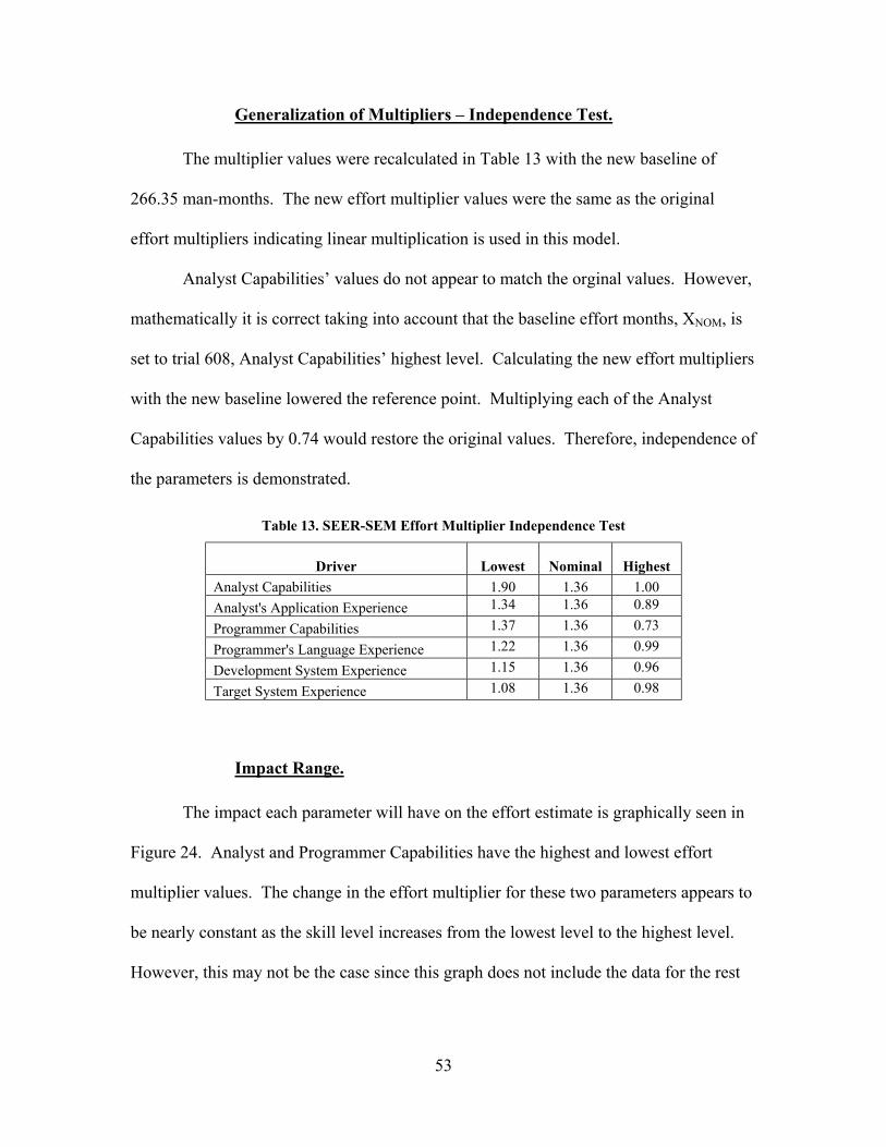
53
Generalization of Multipliers – Independence Test.
The multiplier values were recalculated in Table 13 with the new baseline of
266.35 man-months. The new effort multiplier values were the same as the original
effort multipliers indicating linear multiplication is used in this model.
Analyst Capabilities’ values do not appear to match the orginal values. However,
mathematically it is correct taking into account that the baseline effort months, XNOM, is
set to trial 608, Analyst Capabilities’ highest level. Calculating the new effort multipliers
with the new baseline lowered the reference point. Multiplying each of the Analyst
Capabilities values by 0.74 would restore the original values. Therefore, independence of
the parameters is demonstrated.
Table 13. SEER-SEM Effort Multiplier Independence Test
Driver Lowest Nominal Highest Analyst Capabilities 1.90 1.36 1.00 Analyst's Application Experience 1.34 1.36 0.89
Programmer Capabilities 1.37 1.36 0.73
Programmer's Language Experience 1.22 1.36 0.99
Development System Experience 1.15 1.36 0.96
Target System Experience 1.08 1.36 0.98
Impact Range.
The impact each parameter will have on the effort estimate is graphically seen in
Figure 24. Analyst and Programmer Capabilities have the highest and lowest effort
multiplier values. The change in the effort multiplier for these two parameters appears to
be nearly constant as the skill level increases from the lowest level to the highest level.
However, this may not be the case since this graph does not include the data for the rest

54
of the skill levels. Programmer’s Language, Develop System, and Target System
Experience appear to have minimal impact above the nominal skill level.
SEER-SEM Individual Personnel Parameter Impact
0.600.700.800.901.001.101.201.301.401.50
Lowest Nominal Highest
Skill Level
Effo
rt M
ultip
lier
Analyst Capabilities
Analyst's Application Experience
Programmer Capabilities
Programmer's Language Experience
Development System Experience
Target System Experience
Figure 24. SEER-SEM Personnel Parameters Spider Plot
Calculating the productivity range, Figure 25, for each of the six parameters
reveals the individual parameter impact. Analyst Capabilities and Programmer
Capabilities have nearly equal impact. The Analyst Capabilities value is the same as the
COCOMO II value. However, Programmer Capabilities range has 13 percent more
impact than COCOMO’s Programmer Capabilities parameter.
Productivity Range
1.89
1.51
1.23
1.20
1.10
1.88
0.00 0.50 1.00 1.50 2.00 2.50
Analyst Capabilities
Analyst's Application Experience
Programmer Capabilities
Programmer's Language Experience
Development System Experience
Target System Experience
Figure 25. SEER-SEM Personnel Parameters Productivity Range

55
The impact of the personnel parameters on effort can be seen in Figure 26. This
graph shows the effort estimate results for all 729 trials used in the experiment verses the
corresponding effort multiplier. The highest skill level combination resulted in an effort
estimate that was 44 percent of the nominal estimate. The lowest skill level combination
increased the effort estimate to 387 percent of the nominal estimate. The group
productivity range was calculated to be 8.70.
SEER-SEM Experiment Results
1.00, 361.30
3.87, 1397.34
0.44, 160.77
0
200
400
600
800
1000
1200
1400
1600
0.00 0.50 1.00 1.50 2.00 2.50 3.00 3.50 4.00 4.50Effort Multiplier
Eff
ort M
onth
s
Figure 26. Overall SEER-SEM Personnel Parameters Impact
The effort estimates were distributed from a low of 160.77 to a high of 1,397.34
person-months and corresponding effort multipliers from 0.44 to 3.87 respectively. The
best fit distribution for the effort multipliers was the Pearson5 distribution using the Chi-
Square for Goodness-of-fit, Figure 27.
The cumulative distribution graph shows that 90 percent of the effort multiplier
values are between 0.60 and 2. 45. This information could be used to develop an upward

56
risk adjusted estimate in the event that the personnel information was unknown or
mischaracterized and all other cost driver information was known. The 90 percent
interval was suggested assuming the worst and best skill level would not be realistically
hired.
Pearson5(8.4134, 11.497) Shift=-0.23593
0.0
0.2
0.4
0.6
0.8
1.0
-0.0
5
0.86
1.77
2.68
3.59
4.50
< >5.0% 5.0%90.0%0.604 2.454
BestFit Student VersionFor Academic Use Only
Figure 27. SEER-SEM Personnel Effort Multiplier Data Distribution
Linear/Nonlinear Impact.
The overall calculated impact of the personnel parameters, Figure 28, on the effort
estimate matches the experiment results data in Figure 26. The largest change, 3.87, from
the nominal effort estimate in the experiment results data equaled the product of each
parameter’s maximum effort multiplier values. The minimum effort multiplier values
multiplied together resulted in the lowest effort estimate and smallest change from
nominal. This is another indication that linear multiplication is performed within the

57
model algorithms. Thus, the effort multiplier values can be used as risk factors to adjust
the SEER-SEM estimate if the personnel parameters are unknown.
SEER-SEM Overall Personnel Effort Impact
0.45
1.00
3.89
0.00
1.00
2.00
3.00
4.00
5.00
Maximum Nominal Minimum
Effort Multiplier Values
Ove
rall
Effo
rt M
ultip
lier
Figure 28. Overall SEER-SEM Calculated Personnel Effort Impact
SLIM.
The effort multiplier values calculated for SLIM were similar to the effort
multipliers in COCOMO II. The baseline effort estimate is 254.73 man-months. The
personnel parameters all have the same effort multipliers. However, the independence
test was not satisfied. This indicates SLIM does not use linear multiplication in the
algorithms to account for the impact of the cost drivers. The personnel group
productivity range was calculated to be 34.09. 90 percent of the effort multipliers fell
between 0.74 and 1.26. Results do not support using the calculated effort multipliers as
risk factors unless only one multiplier is used at a time since the parameters are not
independent. Raw experiment data is located in Appendix 9.

58
Effort Multipliers.
Effort multipliers were calculated for each cost driver, Table 14. The results were
very different than those obtained for COCOMO II and SEER-SEM. All six parameters
have the same values; although two parameters, Q3 and Q9, have the effort multipliers
reversed. Q3 measures the staff turnover in the company. This measures the inverse of
COCOMO II’s Personnel Continuity. Thus, the reversal of the multipliers when
compared to COCOMO.
Table 14. SLIM Calculated Effort Multipliers
Question Lowest Nominal Highest
Q1 (Management and Leadership) 1.33 1.00 0.74 Q3 (Staff Turnover) 0.75 1.00 1.35 Q4 (Skilled Manpower) 1.33 1.00 0.74 Q5 (Functional Knowledge) 1.33 1.00 0.74 Q6 (Application Experience) 1.33 1.00 0.74 Q9 (Communication Complexity) 0.75 1.00 1.35
Generalization of Multipliers – Independence Test.
The multiplier values were recalculated in Table 15 with the new baseline of
188.08 man-months. The original effort multipliers were not reproduced. This indicates
that the model does not use linear multiplication. Therefore, the original multipliers
would only be relevant for the input scenario in this experiment. Further analysis would
need to be conducted to characterize the personnel impact in the SLIM model beyond this
scenario.
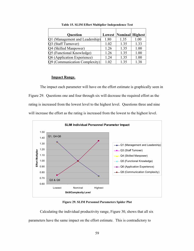
59
Table 15. SLIM Effort Multiplier Independence Test
Question Lowest Nominal Highest Q1 (Management and Leadership) 1.80 1.35 1.00 Q3 (Staff Turnover) 1.02 1.35 1.33 Q4 (Skilled Manpower) 1.26 1.35 1.00 Q5 (Functional Knowledge) 1.26 1.35 1.00 Q6 (Application Experience) 1.24 1.35 1.00 Q9 (Communication Complexity) 1.02 1.35 1.38
Impact Range.
The impact each parameter will have on the effort estimate is graphically seen in
Figure 29. Questions one and four through six will decrease the required effort as the
rating is increased from the lowest level to the highest level. Questions three and nine
will increase the effort as the rating is increased from the lowest to the highest level.
SLIM Individual Personnel Parameter Impact
0.60
0.70
0.80
0.90
1.00
1.10
1.20
1.30
1.40
1.50
Lowest Nominal Highest
Skill/Complexity Level
Effo
rt M
ultip
lier
Q1 (Management and Leadership)
Q3 (Staff Turnover)
Q4 (Skilled Manpower)
Q5 (Functional Knowledge)
Q6 (Application Experience)
Q9 (Communication Complexity)
Q3 & Q9
Q1, Q4-Q6
Figure 29. SLIM Personnel Parameters Spider Plot
Calculating the individual productivity range, Figure 30, shows that all six
parameters have the same impact on the effort estimate. This is contradictory to

60
information in the SLIM-Estimate 5.0 User’s Guide. “Not only do some questions carry
more weight than others do; as your answers approach the opposite ends of the spectrum
(0 or 10), they will have more impact on the PI [Productivity Index]. You will also find
that as you answer more questions, each individual answer has less of an impact on the
final PI” [25:104]. This indicates that the algorithm used to calculate the personnel
impact is very complex.
Productivity Range
1.80
1.80
1.80
1.80
1.80
1.80
0.00 1.00 2.00
Q1 (Management and Leadership)
Q3 (Staff Turnover)
Q4 (Skilled Manpow er)
Q5 (Functional Know ledge)
Q6 (Application Experience)
Q9 (Communication Complexity)
Figure 30. SLIM Personnel Parameters Productivity Range
The impact of the personnel parameters on effort can be seen in Figure 31. The
group productivity range was calculated to be 34.09, indicating twice the impact of
COCOMO II. The actual experiment results do not support the group productivity range.
The highest skill level

61
SLIM Experiment Results
0.57, 145.72
1.00, 254.73
1.35, 345.06
100
150
200
250
300
350
400
0.50 0.60 0.70 0.80 0.90 1.00 1.10 1.20 1.30 1.40Effort Multiplier
Effo
rt (M
an M
onth
s)
Figure 31. Overall SLIM Personnel Parameters Impact
resulted in an effort estimate that was 57 percent of the nominal estimate. The lowest
skill level combination increased the effort estimate to 135 percent of the nominal
estimate. The experiment data would calculate a 2.37 group productivity range. Further
analysis is required to determine if this characterization of the personnel parameters is
valid given that the impact of the individual parameters can change depending on the
number of questions answered.
The effort months were distributed from a low of 145.72 to a high of 345.06
person-months and corresponding effort multipliers from 0.57 to 1.35 respectively.
Using Palisade Decision Tools’ Best Fit 4.5 software, the best fit distribution for the
effort multipliers was the Normal distribution using the Chi-Square for Goodness-of-fit,
Figure 32. The graph shows that 90 percent of the effort multiplier values are between
0.74 and 1.26.
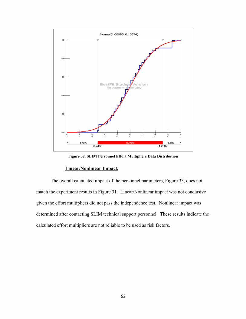
62
Normal(1.00085, 0.15674)
0.0
0.2
0.4
0.6
0.8
1.0
0.5
0.6
0.7
0.8
0.9
1.0
1.1
1.2
1.3
1.4
< >5.0% 5.0%90.0%0.7430 1.2587
BestFit Student VersionFor Academic Use Only
Figure 32. SLIM Personnel Effort Multipliers Data Distribution
Linear/Nonlinear Impact.
The overall calculated impact of the personnel parameters, Figure 33, does not
match the experiment results in Figure 31. Linear/Nonlinear impact was not conclusive
given the effort multipliers did not pass the independence test. Nonlinear impact was
determined after contacting SLIM technical support personnel. These results indicate the
calculated effort multipliers are not reliable to be used as risk factors.

63
SLIM Overall Personnel Effort Impact
5.74
0.171.00
0.001.002.003.004.005.006.007.00
Maximum Nominal Minimum
Effort Multiplier Values
Ove
rall
Effo
rt M
ultip
lier
Figure 33. Overall Calculated SLIM Personnel Effort Impact
For example, if Communication Complexity (Q3) and Staff Turnover (Q9)
parameters were set at the highest setting, the resultant effort multiplier should be 1.82;
the product of 1.35 and 1.35 from Table 14. That combination should increase the
nominal effort estimate from 254.73 to 463.61 man-months.
The calculated effort estimate can be confirmed by checking the actual
experiment data. SLIM experiment run 447, page 140, corresponds to Q3 and Q9 set to
the Hi setting and all other parameters set to nominal. The effort estimate result from
SLIM is 345.06 man-months, not 463.61. The estimate returned by SLIM was the same
effort estimate for Q3 set to Hi and all the other parameters set to nominal, run 446. This
indicates a more complex algorithm than linear multiplication as indicated in the SLIM
user’s guide. The effort multipliers must be used very carefully as risk factors possibly in
isolation from other multipliers given the interaction.

64
PRICE S.
The effort multiplier values calculated for PRICE S were very different from
effort multipliers in COCOMO II. The baseline effort estimate was 1,717.20 man-
months much higher than any of the other models. The personnel parameter with the
most impact was calculated to be CPLX1. The personnel group productivity range was
99.67. 90 percent of the effort multipliers fell between 0.10 and 3.64. Results do not
support using PROFAC effort multipliers as risk factors with CPLX1 and CPLXM. The
raw experiment data is in Appendix 10.
Effort Multipliers.
Effort multipliers were calculated for each personnel parameter, Table 16.
PROFAC increases the required effort when productivity is low. The required effort
decreases as the productivity increases to the highest rating as seen in the decreasing
effort multiplier values. Intuitively, this would be the reverse for CPLX1 and CPLXM
since lower complexity would require less effort as seen in the effort multipliers.CPLX1
would increase the effort estimate by 319 percent when personnel complexity was at the
highest setting.
Table 16. PRICE S Calculated Effort Multipliers
Driver Lowest Nominal Highest
PROFAC 1.10 1.00 0.91 CPLX1 0.07 1.00 3.19 CPLXM 1.00 1.00 1.87
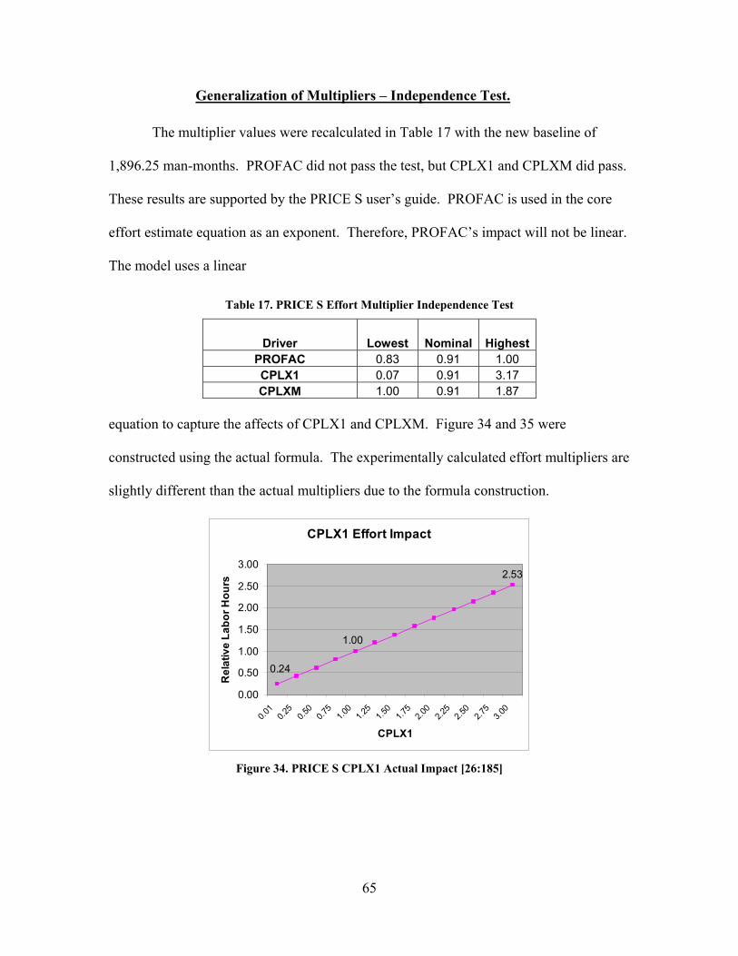
65
Generalization of Multipliers – Independence Test.
The multiplier values were recalculated in Table 17 with the new baseline of
1,896.25 man-months. PROFAC did not pass the test, but CPLX1 and CPLXM did pass.
These results are supported by the PRICE S user’s guide. PROFAC is used in the core
effort estimate equation as an exponent. Therefore, PROFAC’s impact will not be linear.
The model uses a linear
Table 17. PRICE S Effort Multiplier Independence Test
Driver Lowest Nominal Highest PROFAC 0.83 0.91 1.00 CPLX1 0.07 0.91 3.17 CPLXM 1.00 0.91 1.87
equation to capture the affects of CPLX1 and CPLXM. Figure 34 and 35 were
constructed using the actual formula. The experimentally calculated effort multipliers are
slightly different than the actual multipliers due to the formula construction.
CPLX1 Effort Impact
0.24
1.00
2.53
0.00
0.50
1.00
1.50
2.00
2.50
3.00
0.01
0.25
0.50
0.75
1.00
1.25
1.50
1.75
2.00
2.25
2.50
2.75
3.00
CPLX1
Rel
ativ
e La
bor H
ours
Figure 34. PRICE S CPLX1 Actual Impact [26:185]

66
CPLXM Effort Impact
1.00
1.32
1.63
0.90
1.00
1.10
1.20
1.30
1.40
1.50
1.60
1.70
0.01 0.25 0.50 0.75 1.00 1.25 1.50 1.75 2.00 2.25 2.50 2.75 3.00
CPLXM
Rel
ativ
e La
bor H
ours
Figure 35. PRICE S CPLXM Actual Effort Impact [26:188]
Impact Range.
Calculating the individual productivity range, Figure 36, for each of the
parameters reveals that CPLX1 has significantly more impact than the other two
parameters. The fact that CPLX1 has more impact than CPLXM is supported using
Figure 34 and 35. Figure 37 shows that as complexity increases effort increases, but as
productivity increases effort decreases. Figure 37 shows PROFAC as actually a flat line.
These plots for PROFAC are deceptive as to the actual impact PROFAC has on effort.
PRICE S Productivity Range
1.21
44.07
1.87
0.00 10.00 20.00 30.00 40.00 50.00
PROFAC
CPLX1
CPLXM
PRIC
E S
Pers
onne
l Pa
ram
eter
Productivity Range
Figure 36. PRICE S Productivity Range
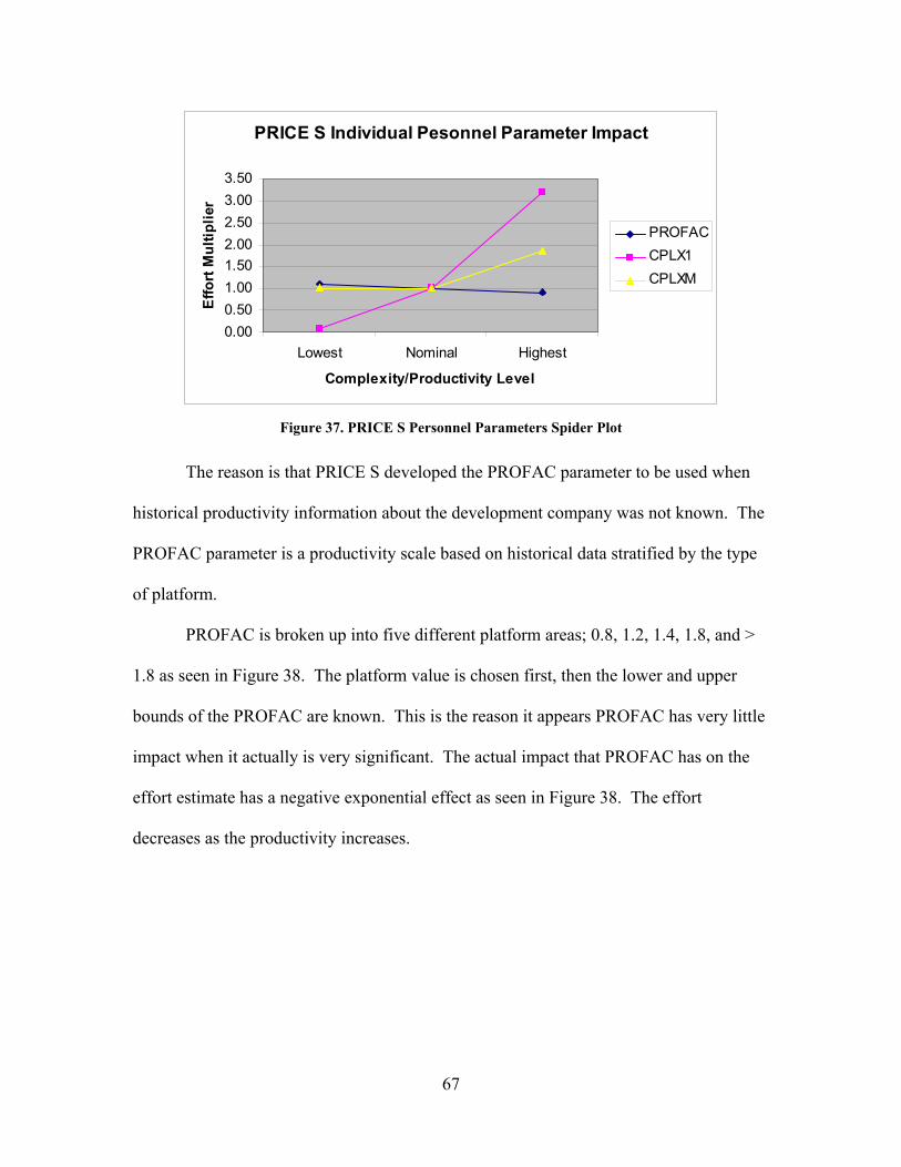
67
PRICE S Individual Pesonnel Parameter Impact
0.000.501.001.502.002.503.003.50
Lowest Nominal Highest
Complexity/Productivity Level
Effo
rt M
ultip
lier
PROFACCPLX1CPLXM
Figure 37. PRICE S Personnel Parameters Spider Plot
The reason is that PRICE S developed the PROFAC parameter to be used when
historical productivity information about the development company was not known. The
PROFAC parameter is a productivity scale based on historical data stratified by the type
of platform.
PROFAC is broken up into five different platform areas; 0.8, 1.2, 1.4, 1.8, and >
1.8 as seen in Figure 38. The platform value is chosen first, then the lower and upper
bounds of the PROFAC are known. This is the reason it appears PROFAC has very little
impact when it actually is very significant. The actual impact that PROFAC has on the
effort estimate has a negative exponential effect as seen in Figure 38. The effort
decreases as the productivity increases.
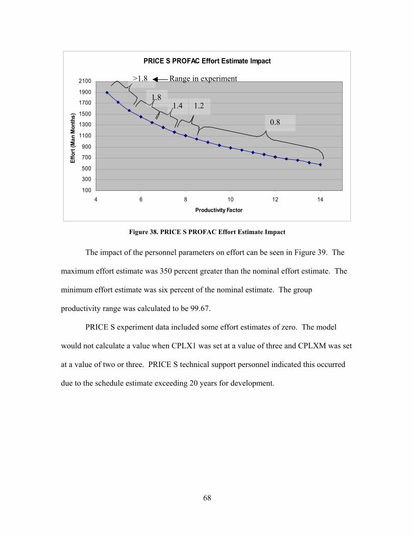
68
PRICE S PROFAC Effort Estimate Impact
100
300
500
700
900
1100
1300
1500
1700
1900
2100
4 6 8 10 12 14
Productivity Factor
Effo
rt (M
an M
onth
s)
Figure 38. PRICE S PROFAC Effort Estimate Impact
The impact of the personnel parameters on effort can be seen in Figure 39. The
maximum effort estimate was 350 percent greater than the nominal effort estimate. The
minimum effort estimate was six percent of the nominal estimate. The group
productivity range was calculated to be 99.67.
PRICE S experiment data included some effort estimates of zero. The model
would not calculate a value when CPLX1 was set at a value of three and CPLXM was set
at a value of two or three. PRICE S technical support personnel indicated this occurred
due to the schedule estimate exceeding 20 years for development.
>1.8
1.8 1.4 1.2
0.8
Range in experiment

69
PRICE S Experiment Results
0.06, 111.61
1.00, 1717.20
3.50, 6012.29
0.00
1000.00
2000.00
3000.00
4000.00
5000.00
6000.00
7000.00
0.00 0.50 1.00 1.50 2.00 2.50 3.00 3.50 4.00
Effort Multiplier
Effo
rt (M
an M
onth
s)
Figure 39. PRICE S Overall Personnel Effort Impact Results
The effort months were distributed from a low of 111.61 to a high of 6,012.29
person-months and corresponding effort multipliers from 0.06 to 3.50 respectively. The
best fit distribution for the effort multipliers was the LogLogistic distribution using the
Chi-Square for Goodness-of-fit, Figure 40. The graph shows that 90 percent of the effort
multiplier combination values are between 0.10 and 3.64.

70
LogLogistic(-0.45011, 1.5022, 2.9374)
0.0
0.2
0.4
0.6
0.8
1.0
-0.5 0.0
0.5
1.0
1.5
2.0
2.5
3.0
3.5
4.0
>5.0% 90.0%0.101 3.643
BestFit Student VersionFor Academic Use Only
Figure 40. PRICE S Personnel Effort Multiplier Distribution
Linear/Nonlinear Impact.
The overall impact of the personnel parameters, Figure 41, on the effort estimate
is just the reverse of the other models since the reverse parameter is being utilized to
calculate the
PRICE S Overall Personnel Effort Impact
1.00
6.58
0.070.00
1.00
2.00
3.00
4.00
5.00
6.00
7.00
Maximum Nominal MinimumEffort Multiplier Values
Ove
rall
Effo
rt M
ultip
lier
Figure 41. Overall PRICE S Personnel Effort Impact

71
impact on effort. The line has a positive slope. This means as the complexity level
increases so does the effort. Overall PROFAC impact is not apparent since only a small
portion of the PROFAC scale was utilized in this experiment scenario. The overall
impact appears to be nonlinear since the slope of the line changes at the nominal level.
Model Comparisons
The objective of this study was to determine the relative change of a cost estimate
from the baseline estimate, XNOM, as personnel parameter input values were altered from
the lowest rating to the highest rating and all other parameters were held constant. The
individual model results explain how each model’s personnel parameters impact the
effort estimate. The results can also be compared to see if the models appear to be
estimating the same development scenario. Figure 42 is a graph of the estimated effort
verses the calculated effort multiplier that shows the relative change
Parameteric Model Personnel Parameter Comparison
0.00
1000.00
2000.00
3000.00
4000.00
5000.00
6000.00
7000.00
0.00 0.50 1.00 1.50 2.00 2.50 3.00 3.50 4.00 4.50
Effort Multiplier
Effo
rt M
onth
s COCOMO IISEER-SEMSLIMPRICE S
Nominal Estimate
PRICE S 1717.20
SEER-SEM 361.30
SLIM 254.73
COCOMO II 169.90
Figure 42. Parametric Model Personnel Comparison

72
The graph shows that COCOMO II, SEER-SEM, and SLIM are estimating very
similar nominal effort results. The nominal values calculated with the initial inputs and
all other parameters set to the nominal setting are noted on the graph. PRICE S appears
to have an initial input that has elevated the nominal effort estimate substantially above
the other three models. This was evaluated with PRICE S personnel. No conclusive
reason was be given that explained the difference in the nominal estimates.
The SLIM results had an anomaly as well. The effort estimates were estimated in
a very tight pattern when compared to the other models. This would lead one to believe
the personnel parameters had little impact on the effort estimate, yet the group
productivity range was twice that of COCOMO II. The explanation given for the tight
pattern results when Quantitative Software Management support personnel were
contacted was that the personnel parameters in the productivity index are impacted by the
size and the initial productivity index value.
Overall Personnel Parameter Impact Comparison
The secondary objective was to use the results of the experiment to develop risk
factors that would enable analysts to develop cost estimate ranges based on the impact of
the subject parameter values. The model’s overall personnel impact graphs would
provide the cost analyst the capability to develop a risk adjusted estimate for each of the
models. Figure 43 shows the maximum and minimum risk range factors. The values for
SLIM and PRICE S are not valid.

73
Parameteric Model Personnel Parameter Impact Comparison
1.001.001.00
6.58
1.00
0.25
4.28
0.45
3.89
0.17
5.74
0.07
-1.00
0.00
1.00
2.00
3.00
4.00
5.00
6.00
7.00
Maximum Nominal Minimum
Effort Multiplier Value Combination
Ove
rall
Effo
rt M
ultip
lier
COCOMO IISEER-SEMSLIMPRICE S
Figure 43. Parametric Model Personnel Parameter Impact Comparison

74
V. Conclusion
Overview
DoD has come to depend on software to improve the capabilities of its weapon
systems. Software performs many tasks formerly executed by a man or woman. Weapon
system capabilities are improved by developing software programs that enhance the
weapon’s ability to perform its intended mission. Increased spending on software has
brought to light the need to manage software costs more closely to ensure resources are
available in the budget to pay for approved programs.
In support of those programs, software cost estimation has evolved from early
back-of-the envelope calculations to a rather complicated process, which has proven
troublesome for accurate cost estimates. Cost estimators use a number of different
methods to construct a software development cost estimate to include commercial
parametric models, analogy, expert opinion, and bottom-up constructive estimates.
Estimates could even be a combination of the methods.
In practice, DoD cost analysts most often use the parametric model method.
Parametric models are fast, require little information to generate an estimate, and are just
as accurate as other methods given the model has been calibrated and validated. The
drawback to most parametric models is that the equations are not published limiting the
cost analysts ability to understand exactly how the model is calculating the estimate.
Many input parameters are based on a qualitative scale. The qualitative scale leaves
room for subjective guessing. The risk of the analyst mischaracterizing the development
environment could jeopardize a program. The program might not be approved if the
estimate is too high or cancelled in the event costs are under estimated. This research is

75
intended to improve the Air Force ability to estimate software development projects by
characterizing to relative importance of personnel parameters. Thus, estimators can
gauge their estimation uncertainty based on their uncertainty about individual personnel
parameters.
This research was conducted using four parametric models widely used in DoD;
COCOMO II, SEER-SEM, SLIM, and PRICE S. Personnel parameters were chosen as
the parameter group to study because literature suggests that personnel abilities impact
the effort more than any factor other than size. The number of personnel inputs to
analyze was reduced down to six since the analysis would include the lowest, nominal,
and highest rating level.
Effort month data was collected from each of the parametric models COCOMO
II, SEER-SEM, SLIM, and PRICE S. The data was analyzed to determine effort
multipliers, independence of parameters, impact range, and linear/nonlinear impact.
COCOMO II data was analyzed first to determine if the methodology could recreate the
COCOMO II published personnel parameters’ effort multipliers. The process was then
repeated for each of the other three model’s results.
Results
The objective of this study was to determine the relative change of a cost estimate
from the baseline estimate as personnel parameter input values were altered from the
lowest rating to the highest rating and all other parameters were held constant. This
objective was accomplished. Additionally, the methodology for evaluating the parameter
impact was validated.

76
The secondary objective was to use the results of the experiment to develop risk
factors that will enable analysts to develop cost estimate ranges based on the uncertainty
and impact of the subject parameter values. Risk factors were calculated for each subject
parameter in each model. These risk factors can be applied under most scenarios with
limitations. Risk ranges can be set for parameters in COCOMO II, SEER-SEM, SLIM,
and PRICE S.
COCOMO II and SEER-SEM personnel effort multipliers can be used as risk
factors without restriction. SLIM parameters were determined to not be independent.
Thus, the risk factors calculated for SLIM cannot be used to determine effort estimates.
PROFAC, one of the parameters in PRICE S, was determined to have a nonlinear impact
on effort possibly skewing the overall impact values. For that reason and because PRICE
S does use linear multiplication to apply the impact of CPLX1 and CPLXM, the
calculated risk factors for CPLX1 and CPLXM are relevant when PROFAC is set at 5.
Thus, PRICE S effort multipliers are only valid in this limited research scenario.
COCOMO II has six personnel parameters. Effort multipliers were calculated for
all six parameters at the lowest and highest setting. The experimentally calculated effort
multipliers matched the values published by Boehm. The baseline effort estimate used to
calculate the COCOMO II effort multipliers was 169.90 man-months. The personnel
parameters with the most impact to effort are Analyst Capability and Programmer
Capability. The personnel group productivity range was 16.90. The effort multipliers
fell between 0.25 and 4.28.
The effort multipliers can be used to develop the risk adjusted estimate for
uncertainty in the personnel parameters. The risk can be applied to individual parameters

77
or the personnel parameters as a group. For example, if the cost analyst is uncertain
about the Analyst Capabilities skill rating, the lowest skill level would change the current
COCOMO II estimate by 142 percent. If the cost analyst felt the development company
had above average Analyst Capabilities, the best skill level would reduce the estimate 29
percent since the effort multiplier is 0.71.
The other scenario is that the cost analyst has no information on the development
company’s individual personnel skills. The only piece of information given is that the
company is above average in personnel skills. The best skill level would be when all the
personnel parameters are rated very high. This combination of effort multiplier values
produces the lowest personnel group multiplier 0.25. Multiplying 0.25 by the current
estimate, 169.90 for example yields 42.48. These manaual calculations can be verified
with the actual model data. The experiment run for the multiplier 0.25 is 729, page 118.
The model estimate was 42.90. The difference is in rounding the group multiplier value
instead of using the product of the individual parameter effort multiplier values.
SEER-SEM has seven personnel parameters. One parameter, Practices and
Methods Experience, was removed since it did not impact the development stage effort
estimate. The effort multiplier values calculated for SEER-SEM were very similar to the
effort multipliers in COCOMO II. The baseline effort estimate was 361.30 man-months.
Just over double COCOMO II’s nominal estimate. The personnel parameters with the
most impact to effort are Analyst Capabilities and Programmer Capabilities. The
personnel group productivity range was 8.70. This means the variance of SEER-SEM
effort multipliers is smaller than COCOMO II. The effort multipliers fell between 0.45
and 3.89.

78
Ensuring the risk factors work for SEER-SEM is important given that the values
are not published by Galorath. The validity of the risk factors can be proven using the
calculated effort multipliers for Analyst Capabilities and Programmer Capabilities at the
lowest skill rating and verifying the results with actual SEER-SEM model data.
However, any of the six parameters used in the experiment could be included.
The Analyst Capabilities and Programmer Capabilities’ values are 1.40 and 1.37
respectively. Multiplying the values together produces 1.92. This value would be the
upper risk bound on the estimate should the actual skill level not be known for Analyst
Capabiltites and Programmer Capabilities. Nominal effort estimate of 361.30 multiplied
by the risk factor of 1.92 results in an upper bound effort estimate of 693.70. This new
estimate can be checked in Appendix 8 for the experiment run where Analyst Capabilities
and Programmer Capabilities are rated low and the other parameters are nominal. The
run number is 95 located on page 115. The values are slightly different due to rounding.
Developing a group risk factor works in a similar fashion. The upper bound risk
factor would be calculated by the product of all the low rating effort multiplier values.
The value would be 3.89. Multiplying 3.89 by 361.30 equals 1,405.46. Looking through
the experiment data for the run with all parameters set to the lowest rating, run 1 page
113, the value is valid.
SLIM uses nine personnel parameters to calculate a productivity index. Six of the
parameters were used in this experiment. The baseline effort estimate was 254.73 man-
months. All the personnel parameters have the same effort multipliers indicating equal
importance. The effort multipliers fell between 0.17 and 5.74. However, the
independence test was not satisfied. This indicates SLIM does not use linear

79
multiplication in the algorithms to account for the impact of the cost drivers. Non-
linearity and parameter interaction was confirmed by SLIM technical support. Therefore,
the second objective was not satisfied for SLIM.
For example, if Communication Complexity (Q3) and Staff Turnover (Q9)
parameters were set at the highest setting, the resultant effort multiplier should be 1.82;
the product of 1.35 and 1.35 from Table 14. That combination should increase the
nominal effort estimate from 254.73 to 463.61 man-months.
The calculated effort estimate can be confirmed by checking the actual
experiment data. SLIM experiment run 447, page 140, corresponds to Q3 and Q9 set to
the Hi setting and all other parameters set to nominal. The effort estimate result from
SLIM is 345.06 man-months, not 463.61. The estimate returned by SLIM was the same
effort estimate for Q3 set to Hi and all the other parameters set to nominal, run 446. This
indicates a more complex algorithm than linear multiplication as indicated in the SLIM
user’s guide rendering the effort multipliers ineffective as risk factors.
PRICE S uses three personnel parameters. Therefore, only 27 different
combinations were analyzed. The baseline effort estimate was 1,717.20 man-months.
The personnel parameters with the most impact to effort appeared to be CPLX1. This
conclusion was incorrect because the range of values used for PROFAC was limited by
the software development scenario. PROFAC was determined to be a nonlinear
parameter, while CPLX1 and CPLXM were linear. Therefore, the effort multipliers for
PROFAC cannot be used to calculate risk ranges. Effort multipliers for CPLX1 and
CPLXM can be used to develop risk ranges. The limitation being that this set of effort
multipliers can only be used when the estimate uses PROFAC set to a value of 5. The

80
personnel group productivity range was 99.6. The effort multipliers fell between 0.07
and 6.58.
These results indicate that parameters other than size can have a significant
impact on the cost estimate. For example, using the SEER-SEM impact ranges, 3.89 to
0.45, and the research scenario, the impact to cost can be shown. The nominal effort
estimate was 361.30 man-months, costing $7,365,100 at $20,385 per man-month. The
upper bound on the cost estimate could be $28,650,241. The lower bound could be
$3,314,295. Thus, the risk of minor to major changes in personnel characterizing can
have a significant impact on overall assessment of program cost.
The cost analyst’s interpretation and qualitative/quantitative characterization of
non-size parameters does or can have a dramatic impact on the estimated effort
translating directly to cost. It is imperative for a cost analyst to gain an appreciation of,
and account for, the potential risk of mis-estimating these parameters!

81
Future Research
This thesis effort developed a methodology for calculating linear effort multipliers
given the model employs linear multiplication. The personnel parameter grouping was
the area analyzed. Future research should explore other parameter groups to develop
effort multipliers for each parameter in the model. Combining the data would generate
an index that could be used to quickly develop risk adjusted estimates. Alternatively, the
non-linear relationships should be explored to better characterize the risk ranges and
possibly fully reverse engineer the models.
Risk adjusted estimates usually mean that an additional cost is anticipated given a
probability of the risk event occurring. The calculated effort multipliers have an assumed
uniform distribution. This is not the case in reality. The risk adjusted estimate could be
further improved if probability data was determined for each qualitative level of the
personnel parameters from completed projects.

82
Appendix 1 COSTAR VBA code
Figure 44. COSTAR Excel file
Sub docostar() ' ' Proof of concept. ' 1) Use values from spreadsheet to create a file of Costar commands ' 2) Execute Costar, writing an ASCII version of a report ' 3) Extract results from the report, put them into spreadsheet ' Dim exe Dim tempdir Dim found Dim i As Integer Dim mystring Dim answer ' ' Find TEMP directory ' tempdir = Environ("TEMP") If tempdir = "" Then tempdir = "c:"

83
If Right(tempdir, 1) <> "\" Then tempdir = tempdir + "\" ' ' Find Costar executable ' exe = "\Program Files\Softstar\Costar 6\costar.exe" found = Dir(exe) If found <> "costar.exe" Then exe = "\Program Files\Softstar\Costar 6.0\costar.exe" found = Dir(exe) End If If found <> "costar.exe" Then exe = "\Program Files\Softstar\Costar 6 Demo\costar.exe" found = Dir(exe) End If If found <> "costar.exe" Then exe = "c:\costar.exe" ' ' Write file of Costar commands ' Open tempdir + "in.cmd" For Output As #1 Print #1, "ACAP "; Worksheets(1).Range("B2").Value Print #1, "dsi "; Worksheets(1).Range("A2").Value Print #1, "print detail "; tempdir + "costar.out" Print #1, "save "; tempdir + "temp.cst" Print #1, "quit" Close #1 ' ' Execute Costar ' RetVal = Shell(exe + " " + tempdir + "in.cmd", vbNormalFocus) ' ' Read Costar results ' Open tempdir + "costar.out" For Input As #1 For i = 1 To 17 Input #1, mystring Next i answer = Mid(mystring, 25, 15) Close #1 Worksheets(1).Range("C2").Value = Val(answer) End Sub

84
Appendix 2 COSTAR Commands.txt file
This is a list of the Costar V4, V5, and V6 commands. From the V4 manual.... =========================================================================== The terms used in the command summary are defined in the following table: Term Definition brkpercent An integer between 0 and 99. cdvalue One of the following: a cost driver rating such as Low or Very high; an effort multiplier such as 1.25; an asterisk ("*"). component-name A 1 to 12 character string. The first character must be a letter (either uppercase or lowercase). The other characters may be letters, numbers, periods, hyphens, or underscores. cost A number between 0 and 99999. ctext A one line comment. database-name A 1 to 12 character string. The first character must be a letter (either uppercase or lowercase). The other characters may be letters, numbers, periods, hyphens, or underscores. delay A number between -9.9 and 99.9. dsivalue A number between 0 and 9999999. estimate-name A 1 to 12 character string. The first character must be a letter (either uppercase or lowercase). The other characters may be letters, numbers, periods, hyphens, or underscores. filename A character string representing a filename. help-name The name of a Costar command, or a special help topic such as "Reports" or "Commands". id A 1 to 4 character string. increment An integer between 1 and 20. mcdvalue One of the following: a cost driver rating such as Low or Very High; an effort multiplier such as 1.25; an asterisk ("*"); an equals sign ("="). milestone An integer between 0 and 6. mode Organic, Semidetached, or Embedded. percent An integer between 0 and 999. pact An integer between 0 and 999. phase An integer between 0 and 4. planning An integer between 0 and 5. report-name The name of the one of the Costar reports. sigma A number between 0.00 and 0.30. startpoint An integer between 0 and 3. svalue Either On or Off. switch The name of one of the Costar switches. Items enclosed in [brackets] are optional parameters. ACAP [cdvalue] [(mcdvalue)] Analyst Capability Cost Driver ACTIVITY Activity Report ADSI dsivalue Set Adapted Delivered Source Instructions APEX [cdvalue] [(mcdvalue)] Applications Experience Cost Driver APM sigma Ada Process Model Conformance ARCHIVE Archive Report CALCMODEL [I] [D] Set Calculation Model CBREAKAGE Cost & Breakage Report CLEF CLEF Report CM percent Set Percent Code Modified COMMENT [ctext] Record Comment for Component COMPONENT component-name Create Component COPY component-name Copy Component COST Cost Profile Report CPI planning Set Conversion Planning Increment CPLX [cdvalue] [(mcdvalue)] Product Complexity Cost Driver CTCOST cost Set Code and Unit Test Cost DATA [cdvalue] [(mcdvalue)] Database Size Cost Driver DBDELETE database-name Delete Database from Memory DBLOAD filename Load Database from File DBSELECT database-name Select Database for Current Estimate DDCOST cost Set Detailed Design Cost DELETE component-name Delete Component DETAIL Detail Report DISPLAY [report-name] [[(]estimate-names[)]] Display Report

85
DM percent Set Percent Design Modified DSI dsivalue Set Delivered Source Instructions EBREAKAGE Effort & Breakage Report ESTCOMMENT [ctext] Record Comment for Current Estimate ESTCOMPARE [estimate-names] Comparison Report ESTCOPY estimate-name Create a Duplicate of Current Estimate ESTCREATE estimate-name Create a New Estimate ESTDELETE estimate-name Delete Estimate from Memory ESTID [id] Assign ID to Current Estimate ESTNAME [estimate-name] Assign Name to Current Estimate ESTSELECT estimate-name Select Current Estimate GCOST Graph Cost vs. Time GMILESTONE Graph Milestones vs. Time GOTO component-name Set New Current Component GSTAFF Graph Staff vs. Time HELP [help-name] Display Help Message ID [id] Assign ID to Current Component IM percent Set Percentage of Integration Required for Modification INCDETAILS Increment Detail Report INCREMENT [increment] Assign Component to an Increment INCSUMMARY Increment Summary Report ITCOST cost Set Integration & Test Cost LEXP [cdvalue] [(mcdvalue)] Programming Language Experience Cost Driver LOAD filename Load Project Estimation Data MNAPM sigma Maintenance Ada Process Model Conformance MNCOST cost Set Maintenance Cost MODE mode Set Development Mode MODP [cdvalue] [(mcdvalue)] Use of Modern Programming Practices Cost Driver MOVE component-name Move Component NAMES Names Report NDSI Set Newly Created Delivered Source Instructions PACT pact Set Percentage Annual Change Traffic PCAP [cdvalue] [(mcdvalue)] Programmer Capability Cost Driver PDCOST cost Set Product Design Cost PRINT report-name [(estimate-names)] [filename] Format Report for Printer PROFILE Write Profile QUIT Exit Program READ Read Commands from File REDRAW Redraw Screen RELY [cdvalue] Required Software Reliability Cost Driver RENAME component-name Rename Current Component RQCOST cost Set Requirements Analysis Cost RUSE [cdvalue] Required Reusability Cost Driver SAVE filename Save Project Estimation Data SCED [cdvalue] Required Development Schedule Cost Driver SCHEDULE Schedule Report SECU [cdvalue] [(mcdvalue)] Classified Security Application Cost Driver SET switch svalue Set Switch SHOW Show Project Hierarchy STAFF Staffing Profile STOR [cdvalue] [(mcdvalue)] Main Storage Constraint Cost Driver STRUCTURE Structure Report SUBCOMPONENT component-name Create Subcomponent SUMMARY Summary Report TIME [cdvalue] [(mcdvalue)] Execution Time Constraint Cost Driver TOOL [cdvalue] [(mcdvalue)] Use of Software Tools Cost Driver TURN [cdvalue] [(mcdvalue)] Computer Turnaround Time Cost Driver USRn [cdvalue] [(mcdvalue)] User Defined Cost Driver VEXP [cdvalue] [(mcdvalue)] Virtual Machine Experience Cost Driver VIRT [cdvalue] [(mcdvalue)] Virtual Machine Volatility Cost Driver VMVH [cdvalue] [(mcdvalue)] Virtual Machine Volatility - Host Cost Driver VMVT [cdvalue] [(mcdvalue)] Virtual Machine Volatility - Target Cost Driver WRITE filename Write Costar Commands to File WSAPM factor weight Worksheet Ada Process Model Conformance WSBREAKAGE increment brkpercent Worksheet Breakage WSCA row column complexity Worksheet Complexity Adjustment WSCOST class year cost Worksheet Labor Cost WSDELAY increment phase delay Worksheet Delay

86
WSDISTRIB phase % % % % % % % Worksheet Labor Distribution WSDSIPFP lines Worksheet DSI per Function Point WSFP factor complexity count Worksheet Function Points WSLANGUAGE language Worksheet Language WSMILESTONE increment milestone Worksheet Milestone WSNAME class name Worksheet Labor Class Name WSPCAF adjustment Worksheet Processing Complexity Adjustment Factor WSSTARTPOINT startpoint Worksheet Startpoint =========================================================================== The annotated commands are new in 5.0. ACAP ACTIVITY ADSI APEX AMCF Annual Maintenance Change Factor. 0..999 APM ARCHIVE ASSESSMENT 0..999 or "a".."e" for the radio buttons 0..8. BRAK Breakage. 0..999 CALCMODEL CBREAKAGE PLEX PEXP LTEX LTEX PCON PCON CD03 SITE CD04 PVOL CD05 DOCU CD06 unused CD07 unused CD08 unused CD09 unused CD90 RCPX CD91 PDIF CD92 PERS CD93 PREX CD94 FCIL CD95 unused CLEF CM COMMENT COMPONENT COPY COST CPI CPLX CTCOST CUTCOST DATA DBDELETE DBLOAD DBSELECT DDCOST DELETE DETAILS DISPLAY DM DSI EBREAKAGE EDSI ESTCOMMENT ESTCOMPARE ESTCOPY ESTCREATE ESTDELETE ESTID ESTIMATE ESTLOAD

87
ESTNAME ESTSELECT EXIT FLEX Scale Driver. 0..7. 0 = Extra Low 7 = Extra Extra High. GOTO GCOST GMILESTONES GSTAFF HELP ID IM INCDETAILS INCREMENT INCSUMMARY ITCOST LEXP LOAD MILESTONES MNCOST MODE MODP MOVE MNAPM MNUNDERSTAND 0..999 or "b".."f" for radio buttons 10..50. MNUNFAMILIAR 0.0..1.0 or "a".."f" for radio buttons 0.0..1.0. NAMES NDSI PACT PARAMETER PCAP PDCOST PMAT Scale Driver. 0..7. 0 = Extra Low 7 = Extra Extra High. PREC Scale Driver. 0..7. 0 = Extra Low 7 = Extra Extra High. PRINT PROFILE QUIT READ REDRAW RELY RENAME RESL Scale Driver. 0..7. 0 = Extra Low 7 = Extra Extra High. RESULTS RQCOST RUSE SAVE SCED SECU STOR SCHEDULE SET SHOW SIZING Sizing report. STAFF STRUCTURE SUBCOMPONENT SUMMARY SWUNDERSTAND 0..999 or "b".."f" for radio buttons 10..50. TEAM Scale Driver. 0..7. 0 = Extra Low 7 = Extra Extra High. TIME TOOL TURN UNFAMILIAR 0.0..1.0 or "a".."f" for radio buttons 0.0..1.0. USR1 USR2 USR3 USR4 USR5 USR6

88
USR7 USR8 USR9 VEXP VIRT VMVH VMVT WRITE WSAPM WSBREAKAGE WSCA WSCOST WSDELAY WSDISTRIB WSDSIPFP WSFP WSLANGUAGE WSMILESTONE WSNAME WSPCAF WSSTARTPOINT =========================================================================== New in V5.... =========================================================================== AMCF Annual Maintenance Change Factor. 0..999 ASSESSMENT 0..999 or "a".."e" for the radio buttons 0..8. BRAK Breakage. 0..999 FLEX Scale Driver. 0..7. 0 = Extra Low 7 = Extra Extra High. MNUNDERSTAND 0..999 or "b".."f" for radio buttons 10..50. MNUNFAMILIAR 0.0..1.0 or "a".."f" for radio buttons 0.0..1.0. PMAT Scale Driver. 0..7. 0 = Extra Low 7 = Extra Extra High. PREC Scale Driver. 0..7. 0 = Extra Low 7 = Extra Extra High. RESL Scale Driver. 0..7. 0 = Extra Low 7 = Extra Extra High. SIZING Sizing report. SWUNDERSTAND 0..999 or "b".."f" for radio buttons 10..50. TEAM Scale Driver. 0..7. 0 = Extra Low 7 = Extra Extra High. UNFAMILIAR 0.0..1.0 or "a".."f" for radio buttons 0.0..1.0. ....new cost drivers (same format as old ones).... =========================================================================== New in V6.... =========================================================================== TXCOST cost Set Taxation Phase Cost MAINTSIZE Sizing report. ===========================================================================

89
Appendix 3 Modified COSTAR VBA code
**Excel workbook must have one worksheet named “Data” and another named “Experiment” **This code is for 6 factors only. Module 1
Option Explicit Public FactorNames(10), FactorLevels(10, 3), NumofFactors As Integer Public NumofLevels As Integer Sub CreateCostarExperimentMatrix() Dim Currentlinecount As Integer Dim RunNumber As Integer, ProjectName As String, i As Integer, j As Integer Dim a As Integer, b As Integer, c As Integer, d As Integer, e As Integer, f As Integer Currentlinecount = 0 RunNumber = 0 Worksheets("Data").Select NumofFactors = Cells(2, 4) NumofLevels = Cells(3, 4) ProjectName = Cells(1, 4) ' ' Read in factor names and levels ' For i = 1 To NumofFactors FactorNames(i) = Cells(i + 4, 3) For j = 1 To 3 FactorLevels(i, j) = Cells(i + 4, 3 + j) Next j Next i Worksheets("Experiment").Select ' ' Create the actual experiment ' Currentlinecount = Currentlinecount + 1 Cells(Currentlinecount, 1) = "Run" Cells(Currentlinecount, 2) = "New Lines of Code" Cells(Currentlinecount, 3) = FactorNames(1) Cells(Currentlinecount, 4) = FactorNames(2) Cells(Currentlinecount, 5) = FactorNames(3) Cells(Currentlinecount, 6) = FactorNames(4) Cells(Currentlinecount, 7) = FactorNames(5) Cells(Currentlinecount, 8) = FactorNames(6) Cells(Currentlinecount, 9) = "Effort Months"

90
For a = 1 To 3 For b = 1 To 3 For c = 1 To 3 For d = 1 To 3 For e = 1 To 3 For f = 1 To 3 Currentlinecount = Currentlinecount + 1 RunNumber = RunNumber + 1 Cells(Currentlinecount, 1) = "Costar " & RunNumber Cells(Currentlinecount, 2) = "40000" Cells(Currentlinecount, 3) = FactorLevels(1, a) Cells(Currentlinecount, 4) = FactorLevels(2, b) Cells(Currentlinecount, 5) = FactorLevels(3, c) Cells(Currentlinecount, 6) = FactorLevels(4, d) Cells(Currentlinecount, 7) = FactorLevels(5, e) Cells(Currentlinecount, 8) = FactorLevels(6, f) Next f Next e Next d Next c Next b Next a ' Run the settings through Costar Call docostar End Sub Module 2 Sub docostar() ' ' Proof of concept. ' 1) Use values from arrays to create a file of Costar commands, "Costar.cmd" ' 2) Execute Costar, writing an ASCII version of a report, "costar.out" ' 3) Extract results from the report, put them into "Experiment" spreadsheet ' Dim exe Dim tempdir Dim found Dim i As Integer, Currentlinecount As Integer Dim mystring Dim answer ' Application.ScreenUpdating = False Currentlinecount = 1 Worksheets("Data").Select NumofFactors = Cells(2, 4) NumofLevels = Cells(3, 4) ' ' Read in factor names and levels ' For i = 1 To NumofFactors
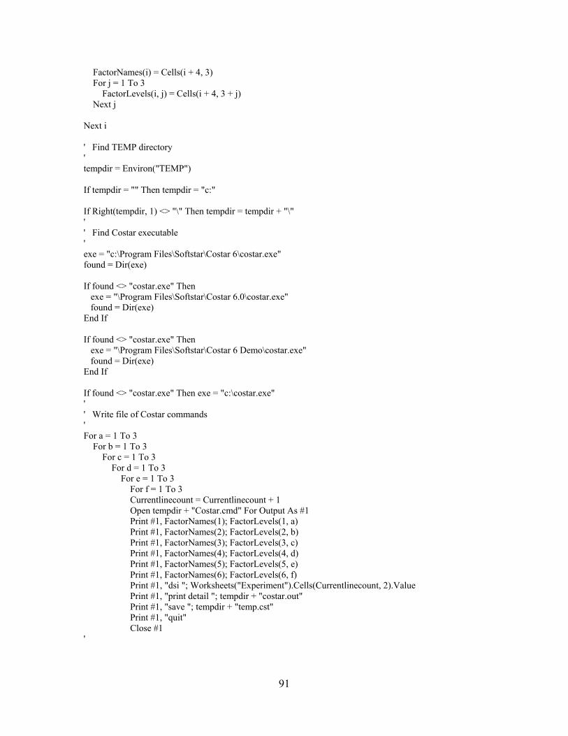
91
FactorNames(i) = Cells(i + 4, 3) For j = 1 To 3 FactorLevels(i, j) = Cells(i + 4, 3 + j) Next j Next i ' Find TEMP directory ' tempdir = Environ("TEMP") If tempdir = "" Then tempdir = "c:" If Right(tempdir, 1) <> "\" Then tempdir = tempdir + "\" ' ' Find Costar executable ' exe = "c:\Program Files\Softstar\Costar 6\costar.exe" found = Dir(exe) If found <> "costar.exe" Then exe = "\Program Files\Softstar\Costar 6.0\costar.exe" found = Dir(exe) End If If found <> "costar.exe" Then exe = "\Program Files\Softstar\Costar 6 Demo\costar.exe" found = Dir(exe) End If If found <> "costar.exe" Then exe = "c:\costar.exe" ' ' Write file of Costar commands ' For a = 1 To 3 For b = 1 To 3 For c = 1 To 3 For d = 1 To 3 For e = 1 To 3 For f = 1 To 3 Currentlinecount = Currentlinecount + 1 Open tempdir + "Costar.cmd" For Output As #1 Print #1, FactorNames(1); FactorLevels(1, a) Print #1, FactorNames(2); FactorLevels(2, b) Print #1, FactorNames(3); FactorLevels(3, c) Print #1, FactorNames(4); FactorLevels(4, d) Print #1, FactorNames(5); FactorLevels(5, e) Print #1, FactorNames(6); FactorLevels(6, f) Print #1, "dsi "; Worksheets("Experiment").Cells(Currentlinecount, 2).Value Print #1, "print detail "; tempdir + "costar.out" Print #1, "save "; tempdir + "temp.cst" Print #1, "quit" Close #1 '

92
' Execute Costar ' RetVal = Shell(exe + " " + tempdir + "costar.cmd", vbNormalFocus) ' ' Read Costar results ' Open tempdir + "costar.out" For Input As #1 For i = 1 To 17 Input #1, mystring Next i answer = Mid(mystring, 25, 15) Close #1 Worksheets("Experiment").Cells(Currentlinecount, 9).Value = Val(answer) Next f Next e Next d Next c Next b Next a End Sub

93
Appendix 4 SEER-SEM VBA Code
Module 1
Sub CreateSeerExperimentMatrix() Dim FactorNames(10) Dim FactorLevels(10, 3) Dim NumofFactors As Integer Dim NumofLevels As Integer Dim Currentlinecount As Integer Dim RunNumber As Integer Currentlinecount = 1 RunNumber = 0 Worksheets("Data").Select NumofFactors = Cells(2, 4) NumofLevels = Cells(3, 4) ProjectName = Cells(1, 4) ' ' Read in factor names and levels ' For i = 1 To NumofFactors FactorNames(i) = Cells(i + 4, 3) For j = 1 To 3 FactorLevels(i, j) = Cells(i + 4, 3 + j) Next j Next i Worksheets("Experiment").Select ' ' Create the actual experiment ' Cells(1, 1) = "ProjectCreate" Cells(1, 2) = "SEER" Cells(1, 3) = ProjectName For a = 1 To 3 For b = 1 To 3 For c = 1 To 3 For d = 1 To 3 For e = 1 To 3 For f = 1 To 3 Currentlinecount = Currentlinecount + 1 RunNumber = RunNumber + 1 Cells(Currentlinecount, 1) = "WBSCreate" Cells(Currentlinecount, 2) = "SEER " & RunNumber Cells(Currentlinecount, 3) = "Program" Cells(Currentlinecount, 4) = "1" Currentlinecount = Currentlinecount + 1 Cells(Currentlinecount, 1) = "New Lines of Code"

94
Cells(Currentlinecount, 2) = "40000" Cells(Currentlinecount, 3) = "40000" Cells(Currentlinecount, 4) = "40000" Currentlinecount = Currentlinecount + 1 Cells(Currentlinecount, 1) = FactorNames(1) Cells(Currentlinecount, 2) = FactorLevels(1, a) Cells(Currentlinecount, 3) = FactorLevels(1, a) Cells(Currentlinecount, 4) = FactorLevels(1, a) Currentlinecount = Currentlinecount + 1 Cells(Currentlinecount, 1) = FactorNames(2) Cells(Currentlinecount, 2) = FactorLevels(2, b) Cells(Currentlinecount, 3) = FactorLevels(2, b) Cells(Currentlinecount, 4) = FactorLevels(2, b) Currentlinecount = Currentlinecount + 1 Cells(Currentlinecount, 1) = FactorNames(3) Cells(Currentlinecount, 2) = FactorLevels(3, c) Cells(Currentlinecount, 3) = FactorLevels(3, c) Cells(Currentlinecount, 4) = FactorLevels(3, c) Currentlinecount = Currentlinecount + 1 Cells(Currentlinecount, 1) = FactorNames(4) Cells(Currentlinecount, 2) = FactorLevels(4, d) Cells(Currentlinecount, 3) = FactorLevels(4, d) Cells(Currentlinecount, 4) = FactorLevels(4, d) Currentlinecount = Currentlinecount + 1 Cells(Currentlinecount, 1) = FactorNames(5) Cells(Currentlinecount, 2) = FactorLevels(5, e) Cells(Currentlinecount, 3) = FactorLevels(5, e) Cells(Currentlinecount, 4) = FactorLevels(5, e) Currentlinecount = Currentlinecount + 1 Cells(Currentlinecount, 1) = FactorNames(6) Cells(Currentlinecount, 2) = FactorLevels(6, f) Cells(Currentlinecount, 3) = FactorLevels(6, f) Cells(Currentlinecount, 4) = FactorLevels(6, f) Next f Next e Next d Next c Next b Next a Currentlinecount = Currentlinecount + 1 Cells(Currentlinecount, 1) = "FlexportOutput" Cells(Currentlinecount, 2) = "SEER DOE" ‘Custom flexible export report to capture parameter values and effort. Cells(Currentlinecount, 3) = "SEER DOE.txt" Currentlinecount = Currentlinecount + 1
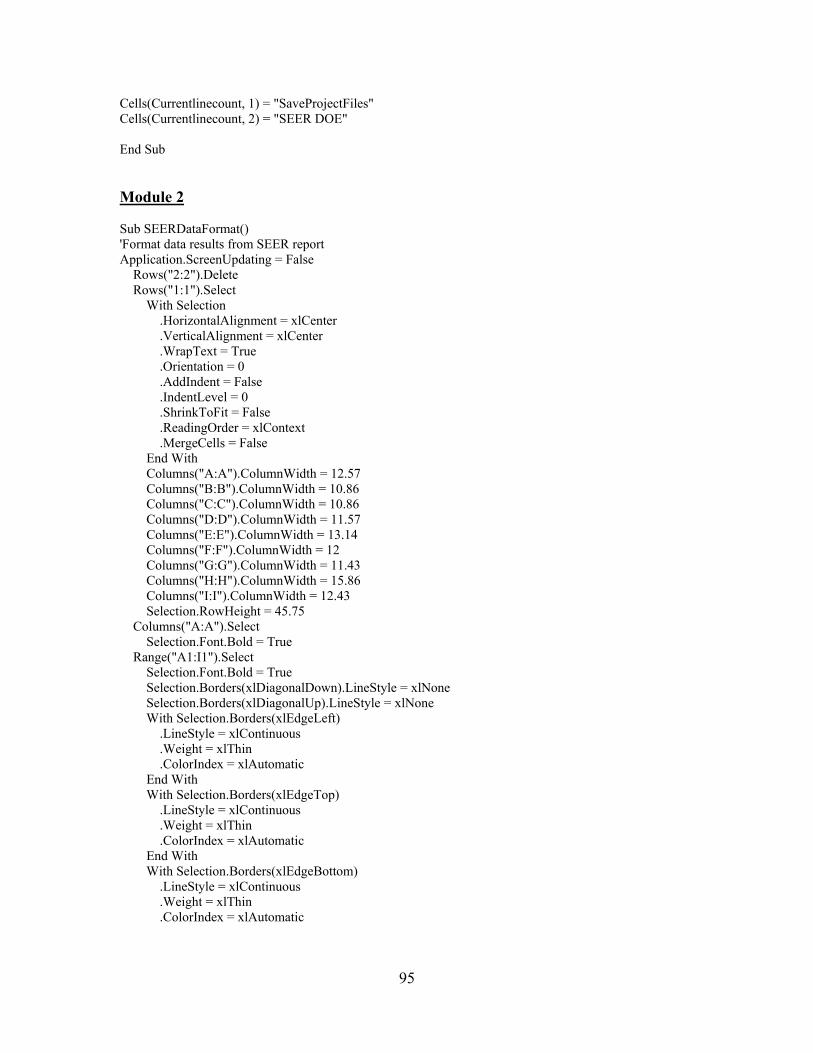
95
Cells(Currentlinecount, 1) = "SaveProjectFiles" Cells(Currentlinecount, 2) = "SEER DOE" End Sub Module 2 Sub SEERDataFormat() 'Format data results from SEER report Application.ScreenUpdating = False Rows("2:2").Delete Rows("1:1").Select With Selection .HorizontalAlignment = xlCenter .VerticalAlignment = xlCenter .WrapText = True .Orientation = 0 .AddIndent = False .IndentLevel = 0 .ShrinkToFit = False .ReadingOrder = xlContext .MergeCells = False End With Columns("A:A").ColumnWidth = 12.57 Columns("B:B").ColumnWidth = 10.86 Columns("C:C").ColumnWidth = 10.86 Columns("D:D").ColumnWidth = 11.57 Columns("E:E").ColumnWidth = 13.14 Columns("F:F").ColumnWidth = 12 Columns("G:G").ColumnWidth = 11.43 Columns("H:H").ColumnWidth = 15.86 Columns("I:I").ColumnWidth = 12.43 Selection.RowHeight = 45.75 Columns("A:A").Select Selection.Font.Bold = True Range("A1:I1").Select Selection.Font.Bold = True Selection.Borders(xlDiagonalDown).LineStyle = xlNone Selection.Borders(xlDiagonalUp).LineStyle = xlNone With Selection.Borders(xlEdgeLeft) .LineStyle = xlContinuous .Weight = xlThin .ColorIndex = xlAutomatic End With With Selection.Borders(xlEdgeTop) .LineStyle = xlContinuous .Weight = xlThin .ColorIndex = xlAutomatic End With With Selection.Borders(xlEdgeBottom) .LineStyle = xlContinuous .Weight = xlThin .ColorIndex = xlAutomatic

96
End With With Selection.Borders(xlEdgeRight) .LineStyle = xlContinuous .Weight = xlThin .ColorIndex = xlAutomatic End With With Selection.Borders(xlInsideVertical) .LineStyle = xlContinuous .Weight = xlThin .ColorIndex = xlAutomatic End With Cells(1, 1).Select End Sub Sub SelectData() With Range("A1") Range(.Cells(1, 1), .End(xlDown).Offset(0, 3)).Copy End With End Sub

97
Appendix 5 SLIM VBA Code
Module 1
Sub CreateSLIMExperimentMatrix() Dim FactorNames(10) Dim FactorLevels(10, 3) Dim NumofFactors As Integer Dim NumofLevels As Integer Dim Currentlinecount As Integer Dim RunNumber As Integer Currentlinecount = 0 RunNumber = 0 Worksheets("Data").Select NumofFactors = Cells(2, 4) NumofLevels = Cells(3, 4) ProjectName = Cells(1, 4) ' ' Read in factor names and levels from Data worksheet ' For i = 1 To NumofFactors FactorNames(i) = Cells(i + 4, 3) For j = 1 To 3 FactorLevels(i, j) = Cells(i + 4, 3 + j) Next j Next i Worksheets("Experiment").Select ' ' Create the actual experiment ' Currentlinecount = Currentlinecount + 1 Cells(Currentlinecount, 1) = "Run" Cells(Currentlinecount, 2) = FactorNames(1) Cells(Currentlinecount, 3) = FactorNames(2) Cells(Currentlinecount, 4) = FactorNames(3) Cells(Currentlinecount, 5) = FactorNames(4) Cells(Currentlinecount, 6) = FactorNames(5) Cells(Currentlinecount, 7) = FactorNames(6) Cells(Currentlinecount, 8) = "Effort Months" Cells(Currentlinecount, 9) = "Change from Nominal" For a = 1 To 3 For b = 1 To 3 For c = 1 To 3 For d = 1 To 3 For e = 1 To 3 For f = 1 To 3

98
Currentlinecount = Currentlinecount + 1 RunNumber = RunNumber + 1 Cells(Currentlinecount, 1) = "SLIM " & RunNumber Cells(Currentlinecount, 2) = FactorLevels(1, a) Cells(Currentlinecount, 3) = FactorLevels(2, b) Cells(Currentlinecount, 4) = FactorLevels(3, c) Cells(Currentlinecount, 5) = FactorLevels(4, d) Cells(Currentlinecount, 6) = FactorLevels(5, e) Cells(Currentlinecount, 7) = FactorLevels(6, f) Next f Next e Next d Next c Next b Next a ' Format Experiment Matrix Range("A1:I1").Select With Selection.Borders(xlEdgeLeft) .LineStyle = xlContinuous .Weight = xlThin .ColorIndex = xlAutomatic End With With Selection.Borders(xlEdgeTop) .LineStyle = xlContinuous .Weight = xlThin .ColorIndex = xlAutomatic End With With Selection.Borders(xlEdgeBottom) .LineStyle = xlContinuous .Weight = xlThin .ColorIndex = xlAutomatic End With With Selection.Borders(xlEdgeRight) .LineStyle = xlContinuous .Weight = xlThin .ColorIndex = xlAutomatic End With With Selection.Borders(xlInsideVertical) .LineStyle = xlContinuous .Weight = xlThin .ColorIndex = xlAutomatic End With With Selection .HorizontalAlignment = xlCenter .VerticalAlignment = xlBottom End With Selection.Font.Bold = True Range("I1").Select With Selection .WrapText = True End With End Sub

99
Appendix 6 PRICE S APPL Values

100

101

102
Appendix 7 COSTAR Data Table
Run ACAP PCAP PCON APEX PLEX LTEX Effort Months
Change from
Nominal
Product of parameter
value
Costar 1 1.42 1.34 1.29 1.22 1.19 1.2 726.40 4.28 4.28 Costar 2 1.42 1.34 1.29 1.22 1.19 1 605.40 3.56 3.56 Costar 3 1.42 1.34 1.29 1.22 1.19 0.84 508.50 2.99 2.99 Costar 4 1.42 1.34 1.29 1.22 1 1.2 610.50 3.59 3.59 Costar 5 1.42 1.34 1.29 1.22 1 1 508.70 2.99 2.99 Costar 6 1.42 1.34 1.29 1.22 1 0.84 427.30 2.52 2.52 Costar 7 1.42 1.34 1.29 1.22 0.85 1.2 518.90 3.05 3.05 Costar 8 1.42 1.34 1.29 1.22 0.85 1 432.40 2.55 2.55 Costar 9 1.42 1.34 1.29 1.22 0.85 0.84 363.20 2.14 2.14 Costar 10 1.42 1.34 1.29 1 1.19 1.2 595.40 3.50 3.51 Costar 11 1.42 1.34 1.29 1 1.19 1 496.20 2.92 2.92 Costar 12 1.42 1.34 1.29 1 1.19 0.84 416.80 2.45 2.45 Costar 13 1.42 1.34 1.29 1 1 1.2 500.40 2.95 2.95 Costar 14 1.42 1.34 1.29 1 1 1 417.00 2.45 2.45 Costar 15 1.42 1.34 1.29 1 1 0.84 350.30 2.06 2.06 Costar 16 1.42 1.34 1.29 1 0.85 1.2 425.30 2.50 2.50 Costar 17 1.42 1.34 1.29 1 0.85 1 354.40 2.09 2.09 Costar 18 1.42 1.34 1.29 1 0.85 0.84 297.70 1.75 1.75 Costar 19 1.42 1.34 1.29 0.81 1.19 1.2 482.30 2.84 2.84 Costar 20 1.42 1.34 1.29 0.81 1.19 1 401.90 2.37 2.37 Costar 21 1.42 1.34 1.29 0.81 1.19 0.84 337.60 1.99 1.99 Costar 22 1.42 1.34 1.29 0.81 1 1.2 405.30 2.39 2.39 Costar 23 1.42 1.34 1.29 0.81 1 1 337.80 1.99 1.99 Costar 24 1.42 1.34 1.29 0.81 1 0.84 283.70 1.67 1.67 Costar 25 1.42 1.34 1.29 0.81 0.85 1.2 344.50 2.03 2.03 Costar 26 1.42 1.34 1.29 0.81 0.85 1 287.10 1.69 1.69 Costar 27 1.42 1.34 1.29 0.81 0.85 0.84 241.20 1.42 1.42 Costar 28 1.42 1.34 1 1.22 1.19 1.2 563.10 3.31 3.31 Costar 29 1.42 1.34 1 1.22 1.19 1 469.30 2.76 2.76 Costar 30 1.42 1.34 1 1.22 1.19 0.84 394.20 2.32 2.32 Costar 31 1.42 1.34 1 1.22 1 1.2 473.20 2.79 2.79 Costar 32 1.42 1.34 1 1.22 1 1 394.40 2.32 2.32 Costar 33 1.42 1.34 1 1.22 1 0.84 331.30 1.95 1.95 Costar 34 1.42 1.34 1 1.22 0.85 1.2 402.20 2.37 2.37 Costar 35 1.42 1.34 1 1.22 0.85 1 335.20 1.97 1.97 Costar 36 1.42 1.34 1 1.22 0.85 0.84 281.60 1.66 1.66 Costar 37 1.42 1.34 1 1 1.19 1.2 461.60 2.72 2.72 Costar 38 1.42 1.34 1 1 1.19 1 384.70 2.26 2.26 Costar 39 1.42 1.34 1 1 1.19 0.84 323.10 1.90 1.90 Costar 40 1.42 1.34 1 1 1 1.2 387.90 2.28 2.28 Costar 41 1.42 1.34 1 1 1 1 323.20 1.90 1.90

103
Run ACAP PCAP PCON APEX PLEX LTEX Effort Months
Change from
Nominal
Product of parameter
value
Costar 42 1.42 1.34 1 1 1 0.84 271.50 1.60 1.60 Costar 43 1.42 1.34 1 1 0.85 1.2 329.70 1.94 1.94 Costar 44 1.42 1.34 1 1 0.85 1 274.80 1.62 1.62 Costar 45 1.42 1.34 1 1 0.85 0.84 230.80 1.36 1.36 Costar 46 1.42 1.34 1 0.81 1.19 1.2 373.90 2.20 2.20 Costar 47 1.42 1.34 1 0.81 1.19 1 311.60 1.83 1.83 Costar 48 1.42 1.34 1 0.81 1.19 0.84 261.70 1.54 1.54 Costar 49 1.42 1.34 1 0.81 1 1.2 314.20 1.85 1.85 Costar 50 1.42 1.34 1 0.81 1 1 261.80 1.54 1.54 Costar 51 1.42 1.34 1 0.81 1 0.84 219.90 1.29 1.29 Costar 52 1.42 1.34 1 0.81 0.85 1.2 267.10 1.57 1.57 Costar 53 1.42 1.34 1 0.81 0.85 1 222.60 1.31 1.31 Costar 54 1.42 1.34 1 0.81 0.85 0.84 186.90 1.10 1.10 Costar 55 1.42 1.34 0.81 1.22 1.19 1.2 456.10 2.68 2.69 Costar 56 1.42 1.34 0.81 1.22 1.19 1 380.10 2.24 2.24 Costar 57 1.42 1.34 0.81 1.22 1.19 0.84 319.30 1.88 1.88 Costar 58 1.42 1.34 0.81 1.22 1 1.2 383.30 2.26 2.26 Costar 59 1.42 1.34 0.81 1.22 1 1 319.40 1.88 1.88 Costar 60 1.42 1.34 0.81 1.22 1 0.84 268.30 1.58 1.58 Costar 61 1.42 1.34 0.81 1.22 0.85 1.2 325.80 1.92 1.92 Costar 62 1.42 1.34 0.81 1.22 0.85 1 271.50 1.60 1.60 Costar 63 1.42 1.34 0.81 1.22 0.85 0.84 228.10 1.34 1.34 Costar 64 1.42 1.34 0.81 1 1.19 1.2 373.90 2.20 2.20 Costar 65 1.42 1.34 0.81 1 1.19 1 311.60 1.83 1.83 Costar 66 1.42 1.34 0.81 1 1.19 0.84 261.70 1.54 1.54 Costar 67 1.42 1.34 0.81 1 1 1.2 314.20 1.85 1.85 Costar 68 1.42 1.34 0.81 1 1 1 261.80 1.54 1.54 Costar 69 1.42 1.34 0.81 1 1 0.84 219.90 1.29 1.29 Costar 70 1.42 1.34 0.81 1 0.85 1.2 267.10 1.57 1.57 Costar 71 1.42 1.34 0.81 1 0.85 1 222.60 1.31 1.31 Costar 72 1.42 1.34 0.81 1 0.85 0.84 186.90 1.10 1.10 Costar 73 1.42 1.34 0.81 0.81 1.19 1.2 302.80 1.78 1.78 Costar 74 1.42 1.34 0.81 0.81 1.19 1 252.40 1.49 1.49 Costar 75 1.42 1.34 0.81 0.81 1.19 0.84 212.00 1.25 1.25 Costar 76 1.42 1.34 0.81 0.81 1 1.2 254.50 1.50 1.50 Costar 77 1.42 1.34 0.81 0.81 1 1 212.10 1.25 1.25 Costar 78 1.42 1.34 0.81 0.81 1 0.84 178.10 1.05 1.05 Costar 79 1.42 1.34 0.81 0.81 0.85 1.2 216.30 1.27 1.27 Costar 80 1.42 1.34 0.81 0.81 0.85 1 180.30 1.06 1.06 Costar 81 1.42 1.34 0.81 0.81 0.85 0.84 151.40 0.89 0.89 Costar 82 1.42 1 1.29 1.22 1.19 1.2 542.10 3.19 3.19 Costar 83 1.42 1 1.29 1.22 1.19 1 451.80 2.66 2.66 Costar 84 1.42 1 1.29 1.22 1.19 0.84 379.50 2.23 2.23 Costar 85 1.42 1 1.29 1.22 1 1.2 455.60 2.68 2.68

104
Run ACAP PCAP PCON APEX PLEX LTEX Effort Months
Change from
Nominal
Product of parameter
value Costar 86 1.42 1 1.29 1.22 1 1 379.60 2.23 2.23 Costar 87 1.42 1 1.29 1.22 1 0.84 318.90 1.88 1.88 Costar 88 1.42 1 1.29 1.22 0.85 1.2 387.20 2.28 2.28 Costar 89 1.42 1 1.29 1.22 0.85 1 322.70 1.90 1.90 Costar 90 1.42 1 1.29 1.22 0.85 0.84 271.10 1.60 1.60 Costar 91 1.42 1 1.29 1 1.19 1.2 444.40 2.62 2.62 Costar 92 1.42 1 1.29 1 1.19 1 370.30 2.18 2.18 Costar 93 1.42 1 1.29 1 1.19 0.84 311.10 1.83 1.83 Costar 94 1.42 1 1.29 1 1 1.2 373.40 2.20 2.20 Costar 95 1.42 1 1.29 1 1 1 311.20 1.83 1.83 Costar 96 1.42 1 1.29 1 1 0.84 261.40 1.54 1.54 Costar 97 1.42 1 1.29 1 0.85 1.2 317.40 1.87 1.87 Costar 98 1.42 1 1.29 1 0.85 1 264.50 1.56 1.56 Costar 99 1.42 1 1.29 1 0.85 0.84 222.20 1.31 1.31 Costar 100 1.42 1 1.29 0.81 1.19 1.2 359.90 2.12 2.12 Costar 101 1.42 1 1.29 0.81 1.19 1 299.90 1.77 1.77 Costar 102 1.42 1 1.29 0.81 1.19 0.84 252.00 1.48 1.48 Costar 103 1.42 1 1.29 0.81 1 1.2 302.50 1.78 1.78 Costar 104 1.42 1 1.29 0.81 1 1 252.10 1.48 1.48 Costar 105 1.42 1 1.29 0.81 1 0.84 211.70 1.25 1.25 Costar 106 1.42 1 1.29 0.81 0.85 1.2 257.10 1.51 1.51 Costar 107 1.42 1 1.29 0.81 0.85 1 214.20 1.26 1.26 Costar 108 1.42 1 1.29 0.81 0.85 0.84 180.00 1.06 1.06 Costar 109 1.42 1 1 1.22 1.19 1.2 420.30 2.47 2.47 Costar 110 1.42 1 1 1.22 1.19 1 350.20 2.06 2.06 Costar 111 1.42 1 1 1.22 1.19 0.84 294.20 1.73 1.73 Costar 112 1.42 1 1 1.22 1 1.2 353.20 2.08 2.08 Costar 113 1.42 1 1 1.22 1 1 294.30 1.73 1.73 Costar 114 1.42 1 1 1.22 1 0.84 247.20 1.45 1.46 Costar 115 1.42 1 1 1.22 0.85 1.2 300.20 1.77 1.77 Costar 116 1.42 1 1 1.22 0.85 1 250.10 1.47 1.47 Costar 117 1.42 1 1 1.22 0.85 0.84 210.10 1.24 1.24 Costar 118 1.42 1 1 1 1.19 1.2 344.50 2.03 2.03 Costar 119 1.42 1 1 1 1.19 1 287.10 1.69 1.69 Costar 120 1.42 1 1 1 1.19 0.84 241.10 1.42 1.42 Costar 121 1.42 1 1 1 1 1.2 289.50 1.70 1.70 Costar 122 1.42 1 1 1 1 1 241.20 1.42 1.42 Costar 123 1.42 1 1 1 1 0.84 202.60 1.19 1.19 Costar 124 1.42 1 1 1 0.85 1.2 246.00 1.45 1.45 Costar 125 1.42 1 1 1 0.85 1 205.00 1.21 1.21 Costar 126 1.42 1 1 1 0.85 0.84 172.20 1.01 1.01 Costar 127 1.42 1 1 0.81 1.19 1.2 279.00 1.64 1.64 Costar 128 1.42 1 1 0.81 1.19 1 232.50 1.37 1.37 Costar 129 1.42 1 1 0.81 1.19 0.84 195.30 1.15 1.15 Costar 130 1.42 1 1 0.81 1 1.2 234.50 1.38 1.38

105
Run ACAP PCAP PCON APEX PLEX LTEX Effort Months
Change from
Nominal
Product of parameter
value Costar 131 1.42 1 1 0.81 1 1 195.40 1.15 1.15 Costar 132 1.42 1 1 0.81 1 0.84 164.10 0.97 0.97 Costar 133 1.42 1 1 0.81 0.85 1.2 199.30 1.17 1.17 Costar 134 1.42 1 1 0.81 0.85 1 166.10 0.98 0.98 Costar 135 1.42 1 1 0.81 0.85 0.84 139.50 0.82 0.82 Costar 136 1.42 1 0.81 1.22 1.19 1.2 340.40 2.00 2.00 Costar 137 1.42 1 0.81 1.22 1.19 1 283.70 1.67 1.67 Costar 138 1.42 1 0.81 1.22 1.19 0.84 238.30 1.40 1.40 Costar 139 1.42 1 0.81 1.22 1 1.2 286.10 1.68 1.68 Costar 140 1.42 1 0.81 1.22 1 1 238.40 1.40 1.40 Costar 141 1.42 1 0.81 1.22 1 0.84 200.20 1.18 1.18 Costar 142 1.42 1 0.81 1.22 0.85 1.2 243.10 1.43 1.43 Costar 143 1.42 1 0.81 1.22 0.85 1 202.60 1.19 1.19 Costar 144 1.42 1 0.81 1.22 0.85 0.84 170.20 1.00 1.00 Costar 145 1.42 1 0.81 1 1.19 1.2 279.00 1.64 1.64 Costar 146 1.42 1 0.81 1 1.19 1 232.50 1.37 1.37 Costar 147 1.42 1 0.81 1 1.19 0.84 195.30 1.15 1.15 Costar 148 1.42 1 0.81 1 1 1.2 234.50 1.38 1.38 Costar 149 1.42 1 0.81 1 1 1 195.40 1.15 1.15 Costar 150 1.42 1 0.81 1 1 0.84 164.10 0.97 0.97 Costar 151 1.42 1 0.81 1 0.85 1.2 199.30 1.17 1.17 Costar 152 1.42 1 0.81 1 0.85 1 166.10 0.98 0.98 Costar 153 1.42 1 0.81 1 0.85 0.84 139.50 0.82 0.82 Costar 154 1.42 1 0.81 0.81 1.19 1.2 226.00 1.33 1.33 Costar 155 1.42 1 0.81 0.81 1.19 1 188.30 1.11 1.11 Costar 156 1.42 1 0.81 0.81 1.19 0.84 158.20 0.93 0.93 Costar 157 1.42 1 0.81 0.81 1 1.2 189.90 1.12 1.12 Costar 158 1.42 1 0.81 0.81 1 1 158.30 0.93 0.93 Costar 159 1.42 1 0.81 0.81 1 0.84 132.90 0.78 0.78 Costar 160 1.42 1 0.81 0.81 0.85 1.2 161.40 0.95 0.95 Costar 161 1.42 1 0.81 0.81 0.85 1 134.50 0.79 0.79 Costar 162 1.42 1 0.81 0.81 0.85 0.84 113.00 0.67 0.67 Costar 163 1.42 0.76 1.29 1.22 1.19 1.2 412.00 2.42 2.43 Costar 164 1.42 0.76 1.29 1.22 1.19 1 343.30 2.02 2.02 Costar 165 1.42 0.76 1.29 1.22 1.19 0.84 288.40 1.70 1.70 Costar 166 1.42 0.76 1.29 1.22 1 1.2 346.20 2.04 2.04 Costar 167 1.42 0.76 1.29 1.22 1 1 288.50 1.70 1.70 Costar 168 1.42 0.76 1.29 1.22 1 0.84 242.40 1.43 1.43 Costar 169 1.42 0.76 1.29 1.22 0.85 1.2 294.30 1.73 1.73 Costar 170 1.42 0.76 1.29 1.22 0.85 1 245.20 1.44 1.44 Costar 171 1.42 0.76 1.29 1.22 0.85 0.84 206.00 1.21 1.21 Costar 172 1.42 0.76 1.29 1 1.19 1.2 337.70 1.99 1.99 Costar 173 1.42 0.76 1.29 1 1.19 1 281.40 1.66 1.66 Costar 174 1.42 0.76 1.29 1 1.19 0.84 236.40 1.39 1.39 Costar 175 1.42 0.76 1.29 1 1 1.2 283.80 1.67 1.67

106
Run ACAP PCAP PCON APEX PLEX LTEX Effort Months
Change from
Nominal
Product of parameter
value Costar 176 1.42 0.76 1.29 1 1 1 236.50 1.39 1.39 Costar 177 1.42 0.76 1.29 1 1 0.84 198.70 1.17 1.17 Costar 178 1.42 0.76 1.29 1 0.85 1.2 241.20 1.42 1.42 Costar 179 1.42 0.76 1.29 1 0.85 1 201.00 1.18 1.18 Costar 180 1.42 0.76 1.29 1 0.85 0.84 168.90 0.99 0.99 Costar 181 1.42 0.76 1.29 0.81 1.19 1.2 273.60 1.61 1.61 Costar 182 1.42 0.76 1.29 0.81 1.19 1 228.00 1.34 1.34 Costar 183 1.42 0.76 1.29 0.81 1.19 0.84 191.50 1.13 1.13 Costar 184 1.42 0.76 1.29 0.81 1 1.2 229.90 1.35 1.35 Costar 185 1.42 0.76 1.29 0.81 1 1 191.60 1.13 1.13 Costar 186 1.42 0.76 1.29 0.81 1 0.84 160.90 0.95 0.95 Costar 187 1.42 0.76 1.29 0.81 0.85 1.2 195.40 1.15 1.15 Costar 188 1.42 0.76 1.29 0.81 0.85 1 162.80 0.96 0.96 Costar 189 1.42 0.76 1.29 0.81 0.85 0.84 136.80 0.81 0.81 Costar 190 1.42 0.76 1 1.22 1.19 1.2 319.40 1.88 1.88 Costar 191 1.42 0.76 1 1.22 1.19 1 266.20 1.57 1.57 Costar 192 1.42 0.76 1 1.22 1.19 0.84 223.60 1.32 1.32 Costar 193 1.42 0.76 1 1.22 1 1.2 268.40 1.58 1.58 Costar 194 1.42 0.76 1 1.22 1 1 223.70 1.32 1.32 Costar 195 1.42 0.76 1 1.22 1 0.84 187.90 1.11 1.11 Costar 196 1.42 0.76 1 1.22 0.85 1.2 228.10 1.34 1.34 Costar 197 1.42 0.76 1 1.22 0.85 1 190.10 1.12 1.12 Costar 198 1.42 0.76 1 1.22 0.85 0.84 159.70 0.94 0.94 Costar 199 1.42 0.76 1 1 1.19 1.2 261.80 1.54 1.54 Costar 200 1.42 0.76 1 1 1.19 1 218.20 1.28 1.28 Costar 201 1.42 0.76 1 1 1.19 0.84 183.30 1.08 1.08 Costar 202 1.42 0.76 1 1 1 1.2 220.00 1.29 1.30 Costar 203 1.42 0.76 1 1 1 1 183.30 1.08 1.08 Costar 204 1.42 0.76 1 1 1 0.84 154.00 0.91 0.91 Costar 205 1.42 0.76 1 1 0.85 1.2 187.00 1.10 1.10 Costar 206 1.42 0.76 1 1 0.85 1 155.80 0.92 0.92 Costar 207 1.42 0.76 1 1 0.85 0.84 130.90 0.77 0.77 Costar 208 1.42 0.76 1 0.81 1.19 1.2 212.10 1.25 1.25 Costar 209 1.42 0.76 1 0.81 1.19 1 176.70 1.04 1.04 Costar 210 1.42 0.76 1 0.81 1.19 0.84 148.40 0.87 0.87 Costar 211 1.42 0.76 1 0.81 1 1.2 178.20 1.05 1.05 Costar 212 1.42 0.76 1 0.81 1 1 148.50 0.87 0.87 Costar 213 1.42 0.76 1 0.81 1 0.84 124.70 0.73 0.73 Costar 214 1.42 0.76 1 0.81 0.85 1.2 151.50 0.89 0.89 Costar 215 1.42 0.76 1 0.81 0.85 1 126.20 0.74 0.74 Costar 216 1.42 0.76 1 0.81 0.85 0.84 106.00 0.62 0.62 Costar 217 1.42 0.76 0.81 1.22 1.19 1.2 258.70 1.52 1.52 Costar 218 1.42 0.76 0.81 1.22 1.19 1 215.60 1.27 1.27 Costar 219 1.42 0.76 0.81 1.22 1.19 0.84 181.10 1.07 1.07 Costar 220 1.42 0.76 0.81 1.22 1 1.2 217.40 1.28 1.28
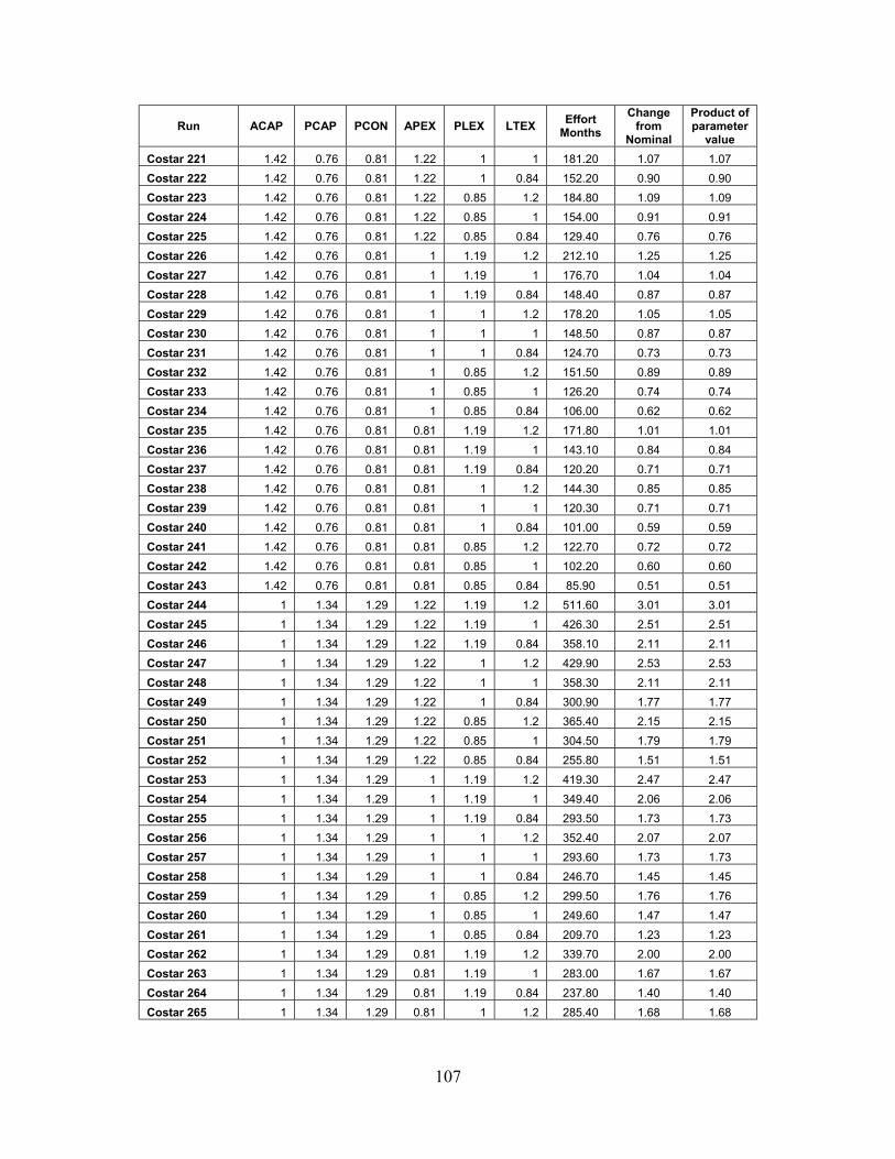
107
Run ACAP PCAP PCON APEX PLEX LTEX Effort Months
Change from
Nominal
Product of parameter
value Costar 221 1.42 0.76 0.81 1.22 1 1 181.20 1.07 1.07 Costar 222 1.42 0.76 0.81 1.22 1 0.84 152.20 0.90 0.90 Costar 223 1.42 0.76 0.81 1.22 0.85 1.2 184.80 1.09 1.09 Costar 224 1.42 0.76 0.81 1.22 0.85 1 154.00 0.91 0.91 Costar 225 1.42 0.76 0.81 1.22 0.85 0.84 129.40 0.76 0.76 Costar 226 1.42 0.76 0.81 1 1.19 1.2 212.10 1.25 1.25 Costar 227 1.42 0.76 0.81 1 1.19 1 176.70 1.04 1.04 Costar 228 1.42 0.76 0.81 1 1.19 0.84 148.40 0.87 0.87 Costar 229 1.42 0.76 0.81 1 1 1.2 178.20 1.05 1.05 Costar 230 1.42 0.76 0.81 1 1 1 148.50 0.87 0.87 Costar 231 1.42 0.76 0.81 1 1 0.84 124.70 0.73 0.73 Costar 232 1.42 0.76 0.81 1 0.85 1.2 151.50 0.89 0.89 Costar 233 1.42 0.76 0.81 1 0.85 1 126.20 0.74 0.74 Costar 234 1.42 0.76 0.81 1 0.85 0.84 106.00 0.62 0.62 Costar 235 1.42 0.76 0.81 0.81 1.19 1.2 171.80 1.01 1.01 Costar 236 1.42 0.76 0.81 0.81 1.19 1 143.10 0.84 0.84 Costar 237 1.42 0.76 0.81 0.81 1.19 0.84 120.20 0.71 0.71 Costar 238 1.42 0.76 0.81 0.81 1 1.2 144.30 0.85 0.85 Costar 239 1.42 0.76 0.81 0.81 1 1 120.30 0.71 0.71 Costar 240 1.42 0.76 0.81 0.81 1 0.84 101.00 0.59 0.59 Costar 241 1.42 0.76 0.81 0.81 0.85 1.2 122.70 0.72 0.72 Costar 242 1.42 0.76 0.81 0.81 0.85 1 102.20 0.60 0.60 Costar 243 1.42 0.76 0.81 0.81 0.85 0.84 85.90 0.51 0.51 Costar 244 1 1.34 1.29 1.22 1.19 1.2 511.60 3.01 3.01 Costar 245 1 1.34 1.29 1.22 1.19 1 426.30 2.51 2.51 Costar 246 1 1.34 1.29 1.22 1.19 0.84 358.10 2.11 2.11 Costar 247 1 1.34 1.29 1.22 1 1.2 429.90 2.53 2.53 Costar 248 1 1.34 1.29 1.22 1 1 358.30 2.11 2.11 Costar 249 1 1.34 1.29 1.22 1 0.84 300.90 1.77 1.77 Costar 250 1 1.34 1.29 1.22 0.85 1.2 365.40 2.15 2.15 Costar 251 1 1.34 1.29 1.22 0.85 1 304.50 1.79 1.79 Costar 252 1 1.34 1.29 1.22 0.85 0.84 255.80 1.51 1.51 Costar 253 1 1.34 1.29 1 1.19 1.2 419.30 2.47 2.47 Costar 254 1 1.34 1.29 1 1.19 1 349.40 2.06 2.06 Costar 255 1 1.34 1.29 1 1.19 0.84 293.50 1.73 1.73 Costar 256 1 1.34 1.29 1 1 1.2 352.40 2.07 2.07 Costar 257 1 1.34 1.29 1 1 1 293.60 1.73 1.73 Costar 258 1 1.34 1.29 1 1 0.84 246.70 1.45 1.45 Costar 259 1 1.34 1.29 1 0.85 1.2 299.50 1.76 1.76 Costar 260 1 1.34 1.29 1 0.85 1 249.60 1.47 1.47 Costar 261 1 1.34 1.29 1 0.85 0.84 209.70 1.23 1.23 Costar 262 1 1.34 1.29 0.81 1.19 1.2 339.70 2.00 2.00 Costar 263 1 1.34 1.29 0.81 1.19 1 283.00 1.67 1.67 Costar 264 1 1.34 1.29 0.81 1.19 0.84 237.80 1.40 1.40 Costar 265 1 1.34 1.29 0.81 1 1.2 285.40 1.68 1.68

108
Run ACAP PCAP PCON APEX PLEX LTEX Effort Months
Change from
Nominal
Product of parameter
value Costar 266 1 1.34 1.29 0.81 1 1 237.90 1.40 1.40 Costar 267 1 1.34 1.29 0.81 1 0.84 199.80 1.18 1.18 Costar 268 1 1.34 1.29 0.81 0.85 1.2 242.60 1.43 1.43 Costar 269 1 1.34 1.29 0.81 0.85 1 202.20 1.19 1.19 Costar 270 1 1.34 1.29 0.81 0.85 0.84 169.80 1.00 1.00 Costar 271 1 1.34 1 1.22 1.19 1.2 396.60 2.33 2.33 Costar 272 1 1.34 1 1.22 1.19 1 330.50 1.95 1.95 Costar 273 1 1.34 1 1.22 1.19 0.84 277.60 1.63 1.63 Costar 274 1 1.34 1 1.22 1 1.2 333.30 1.96 1.96 Costar 275 1 1.34 1 1.22 1 1 277.70 1.63 1.63 Costar 276 1 1.34 1 1.22 1 0.84 233.30 1.37 1.37 Costar 277 1 1.34 1 1.22 0.85 1.2 283.30 1.67 1.67 Costar 278 1 1.34 1 1.22 0.85 1 236.10 1.39 1.39 Costar 279 1 1.34 1 1.22 0.85 0.84 198.30 1.17 1.17 Costar 280 1 1.34 1 1 1.19 1.2 325.10 1.91 1.91 Costar 281 1 1.34 1 1 1.19 1 270.90 1.59 1.59 Costar 282 1 1.34 1 1 1.19 0.84 227.50 1.34 1.34 Costar 283 1 1.34 1 1 1 1.2 273.20 1.61 1.61 Costar 284 1 1.34 1 1 1 1 227.60 1.34 1.34 Costar 285 1 1.34 1 1 1 0.84 191.20 1.13 1.13 Costar 286 1 1.34 1 1 0.85 1.2 232.20 1.37 1.37 Costar 287 1 1.34 1 1 0.85 1 193.50 1.14 1.14 Costar 288 1 1.34 1 1 0.85 0.84 162.50 0.96 0.96 Costar 289 1 1.34 1 0.81 1.19 1.2 263.30 1.55 1.55 Costar 290 1 1.34 1 0.81 1.19 1 219.40 1.29 1.29 Costar 291 1 1.34 1 0.81 1.19 0.84 184.30 1.08 1.08 Costar 292 1 1.34 1 0.81 1 1.2 221.30 1.30 1.30 Costar 293 1 1.34 1 0.81 1 1 184.40 1.09 1.09 Costar 294 1 1.34 1 0.81 1 0.84 154.90 0.91 0.91 Costar 295 1 1.34 1 0.81 0.85 1.2 188.10 1.11 1.11 Costar 296 1 1.34 1 0.81 0.85 1 156.70 0.92 0.92 Costar 297 1 1.34 1 0.81 0.85 0.84 131.60 0.77 0.77 Costar 298 1 1.34 0.81 1.22 1.19 1.2 321.20 1.89 1.89 Costar 299 1 1.34 0.81 1.22 1.19 1 267.70 1.58 1.58 Costar 300 1 1.34 0.81 1.22 1.19 0.84 224.90 1.32 1.32 Costar 301 1 1.34 0.81 1.22 1 1.2 269.90 1.59 1.59 Costar 302 1 1.34 0.81 1.22 1 1 224.90 1.32 1.32 Costar 303 1 1.34 0.81 1.22 1 0.84 189.00 1.11 1.11 Costar 304 1 1.34 0.81 1.22 0.85 1.2 229.40 1.35 1.35 Costar 305 1 1.34 0.81 1.22 0.85 1 191.20 1.13 1.13 Costar 306 1 1.34 0.81 1.22 0.85 0.84 160.60 0.95 0.95 Costar 307 1 1.34 0.81 1 1.19 1.2 263.30 1.55 1.55 Costar 308 1 1.34 0.81 1 1.19 1 219.40 1.29 1.29 Costar 309 1 1.34 0.81 1 1.19 0.84 184.30 1.08 1.08 Costar 310 1 1.34 0.81 1 1 1.2 221.30 1.30 1.30

109
Run ACAP PCAP PCON APEX PLEX LTEX Effort Months
Change from
Nominal
Product of parameter
value Costar 311 1 1.34 0.81 1 1 1 184.40 1.09 1.09 Costar 312 1 1.34 0.81 1 1 0.84 154.90 0.91 0.91 Costar 313 1 1.34 0.81 1 0.85 1.2 188.10 1.11 1.11 Costar 314 1 1.34 0.81 1 0.85 1 156.70 0.92 0.92 Costar 315 1 1.34 0.81 1 0.85 0.84 131.60 0.77 0.77 Costar 316 1 1.34 0.81 0.81 1.19 1.2 213.30 1.26 1.26 Costar 317 1 1.34 0.81 0.81 1.19 1 177.70 1.05 1.05 Costar 318 1 1.34 0.81 0.81 1.19 0.84 149.30 0.88 0.88 Costar 319 1 1.34 0.81 0.81 1 1.2 179.20 1.05 1.06 Costar 320 1 1.34 0.81 0.81 1 1 149.40 0.88 0.88 Costar 321 1 1.34 0.81 0.81 1 0.84 125.50 0.74 0.74 Costar 322 1 1.34 0.81 0.81 0.85 1.2 152.30 0.90 0.90 Costar 323 1 1.34 0.81 0.81 0.85 1 126.90 0.75 0.75 Costar 324 1 1.34 0.81 0.81 0.85 0.84 106.60 0.63 0.63 Costar 325 1 1 1.29 1.22 1.19 1.2 381.80 2.25 2.25 Costar 326 1 1 1.29 1.22 1.19 1 318.10 1.87 1.87 Costar 327 1 1 1.29 1.22 1.19 0.84 267.20 1.57 1.57 Costar 328 1 1 1.29 1.22 1 1.2 320.80 1.89 1.89 Costar 329 1 1 1.29 1.22 1 1 267.40 1.57 1.57 Costar 330 1 1 1.29 1.22 1 0.84 224.60 1.32 1.32 Costar 331 1 1 1.29 1.22 0.85 1.2 272.70 1.61 1.61 Costar 332 1 1 1.29 1.22 0.85 1 227.20 1.34 1.34 Costar 333 1 1 1.29 1.22 0.85 0.84 190.90 1.12 1.12 Costar 334 1 1 1.29 1 1.19 1.2 312.90 1.84 1.84 Costar 335 1 1 1.29 1 1.19 1 260.80 1.54 1.54 Costar 336 1 1 1.29 1 1.19 0.84 219.10 1.29 1.29 Costar 337 1 1 1.29 1 1 1.2 263.00 1.55 1.55 Costar 338 1 1 1.29 1 1 1 219.10 1.29 1.29 Costar 339 1 1 1.29 1 1 0.84 184.10 1.08 1.08 Costar 340 1 1 1.29 1 0.85 1.2 223.50 1.32 1.32 Costar 341 1 1 1.29 1 0.85 1 186.30 1.10 1.10 Costar 342 1 1 1.29 1 0.85 0.84 156.50 0.92 0.92 Costar 343 1 1 1.29 0.81 1.19 1.2 253.50 1.49 1.49 Costar 344 1 1 1.29 0.81 1.19 1 211.20 1.24 1.24 Costar 345 1 1 1.29 0.81 1.19 0.84 177.40 1.04 1.04 Costar 346 1 1 1.29 0.81 1 1.2 213.00 1.25 1.25 Costar 347 1 1 1.29 0.81 1 1 177.50 1.04 1.04 Costar 348 1 1 1.29 0.81 1 0.84 149.10 0.88 0.88 Costar 349 1 1 1.29 0.81 0.85 1.2 181.10 1.07 1.07 Costar 350 1 1 1.29 0.81 0.85 1 150.90 0.89 0.89 Costar 351 1 1 1.29 0.81 0.85 0.84 126.70 0.75 0.75 Costar 352 1 1 1 1.22 1.19 1.2 296.00 1.74 1.74 Costar 353 1 1 1 1.22 1.19 1 246.60 1.45 1.45 Costar 354 1 1 1 1.22 1.19 0.84 207.20 1.22 1.22 Costar 355 1 1 1 1.22 1 1.2 248.70 1.46 1.46

110
Run ACAP PCAP PCON APEX PLEX LTEX Effort Months
Change from
Nominal
Product of parameter
value Costar 356 1 1 1 1.22 1 1 207.20 1.22 1.22 Costar 357 1 1 1 1.22 1 0.84 174.10 1.02 1.02 Costar 358 1 1 1 1.22 0.85 1.2 211.40 1.24 1.24 Costar 359 1 1 1 1.22 0.85 1 176.20 1.04 1.04 Costar 360 1 1 1 1.22 0.85 0.84 148.00 0.87 0.87 Costar 361 1 1 1 1 1.19 1.2 242.60 1.43 1.43 Costar 362 1 1 1 1 1.19 1 202.20 1.19 1.19 Costar 363 1 1 1 1 1.19 0.84 169.80 1.00 1.00 Costar 364 1 1 1 1 1 1.2 203.90 1.20 1.20 Costar 365 1 1 1 1 1 1 169.90 1.00 1.00 Costar 366 1 1 1 1 1 0.84 142.70 0.84 0.84 Costar 367 1 1 1 1 0.85 1.2 173.30 1.02 1.02 Costar 368 1 1 1 1 0.85 1 144.40 0.85 0.85 Costar 369 1 1 1 1 0.85 0.84 121.30 0.71 0.71 Costar 370 1 1 1 0.81 1.19 1.2 196.50 1.16 1.16 Costar 371 1 1 1 0.81 1.19 1 163.70 0.96 0.96 Costar 372 1 1 1 0.81 1.19 0.84 137.50 0.81 0.81 Costar 373 1 1 1 0.81 1 1.2 165.10 0.97 0.97 Costar 374 1 1 1 0.81 1 1 137.60 0.81 0.81 Costar 375 1 1 1 0.81 1 0.84 115.60 0.68 0.68 Costar 376 1 1 1 0.81 0.85 1.2 140.40 0.83 0.83 Costar 377 1 1 1 0.81 0.85 1 117.00 0.69 0.69 Costar 378 1 1 1 0.81 0.85 0.84 98.20 0.58 0.58 Costar 379 1 1 0.81 1.22 1.19 1.2 239.70 1.41 1.41 Costar 380 1 1 0.81 1.22 1.19 1 199.80 1.18 1.18 Costar 381 1 1 0.81 1.22 1.19 0.84 167.80 0.99 0.99 Costar 382 1 1 0.81 1.22 1 1.2 201.40 1.19 1.19 Costar 383 1 1 0.81 1.22 1 1 167.90 0.99 0.99 Costar 384 1 1 0.81 1.22 1 0.84 141.00 0.83 0.83 Costar 385 1 1 0.81 1.22 0.85 1.2 171.20 1.01 1.01 Costar 386 1 1 0.81 1.22 0.85 1 142.70 0.84 0.84 Costar 387 1 1 0.81 1.22 0.85 0.84 119.90 0.71 0.71 Costar 388 1 1 0.81 1 1.19 1.2 196.50 1.16 1.16 Costar 389 1 1 0.81 1 1.19 1 163.70 0.96 0.96 Costar 390 1 1 0.81 1 1.19 0.84 137.50 0.81 0.81 Costar 391 1 1 0.81 1 1 1.2 165.10 0.97 0.97 Costar 392 1 1 0.81 1 1 1 137.60 0.81 0.81 Costar 393 1 1 0.81 1 1 0.84 115.60 0.68 0.68 Costar 394 1 1 0.81 1 0.85 1.2 140.40 0.83 0.83 Costar 395 1 1 0.81 1 0.85 1 117.00 0.69 0.69 Costar 396 1 1 0.81 1 0.85 0.84 98.20 0.58 0.58 Costar 397 1 1 0.81 0.81 1.19 1.2 159.20 0.94 0.94 Costar 398 1 1 0.81 0.81 1.19 1 132.60 0.78 0.78 Costar 399 1 1 0.81 0.81 1.19 0.84 111.40 0.66 0.66 Costar 400 1 1 0.81 0.81 1 1.2 133.70 0.79 0.79

111
Run ACAP PCAP PCON APEX PLEX LTEX Effort Months
Change from
Nominal
Product of parameter
value Costar 401 1 1 0.81 0.81 1 1 111.50 0.66 0.66 Costar 402 1 1 0.81 0.81 1 0.84 93.60 0.55 0.55 Costar 403 1 1 0.81 0.81 0.85 1.2 113.70 0.67 0.67 Costar 404 1 1 0.81 0.81 0.85 1 94.70 0.56 0.56 Costar 405 1 1 0.81 0.81 0.85 0.84 79.60 0.47 0.47 Costar 406 1 0.76 1.29 1.22 1.19 1.2 290.20 1.71 1.71 Costar 407 1 0.76 1.29 1.22 1.19 1 241.80 1.42 1.42 Costar 408 1 0.76 1.29 1.22 1.19 0.84 203.10 1.20 1.20 Costar 409 1 0.76 1.29 1.22 1 1.2 243.80 1.43 1.44 Costar 410 1 0.76 1.29 1.22 1 1 203.20 1.20 1.20 Costar 411 1 0.76 1.29 1.22 1 0.84 170.70 1.00 1.00 Costar 412 1 0.76 1.29 1.22 0.85 1.2 207.30 1.22 1.22 Costar 413 1 0.76 1.29 1.22 0.85 1 172.70 1.02 1.02 Costar 414 1 0.76 1.29 1.22 0.85 0.84 145.10 0.85 0.85 Costar 415 1 0.76 1.29 1 1.19 1.2 237.80 1.40 1.40 Costar 416 1 0.76 1.29 1 1.19 1 198.20 1.17 1.17 Costar 417 1 0.76 1.29 1 1.19 0.84 166.50 0.98 0.98 Costar 418 1 0.76 1.29 1 1 1.2 199.90 1.18 1.18 Costar 419 1 0.76 1.29 1 1 1 166.50 0.98 0.98 Costar 420 1 0.76 1.29 1 1 0.84 139.90 0.82 0.82 Costar 421 1 0.76 1.29 1 0.85 1.2 169.90 1.00 1.00 Costar 422 1 0.76 1.29 1 0.85 1 141.60 0.83 0.83 Costar 423 1 0.76 1.29 1 0.85 0.84 118.90 0.70 0.70 Costar 424 1 0.76 1.29 0.81 1.19 1.2 192.60 1.13 1.13 Costar 425 1 0.76 1.29 0.81 1.19 1 160.50 0.94 0.95 Costar 426 1 0.76 1.29 0.81 1.19 0.84 134.80 0.79 0.79 Costar 427 1 0.76 1.29 0.81 1 1.2 161.90 0.95 0.95 Costar 428 1 0.76 1.29 0.81 1 1 134.90 0.79 0.79 Costar 429 1 0.76 1.29 0.81 1 0.84 113.30 0.67 0.67 Costar 430 1 0.76 1.29 0.81 0.85 1.2 137.60 0.81 0.81 Costar 431 1 0.76 1.29 0.81 0.85 1 114.70 0.68 0.68 Costar 432 1 0.76 1.29 0.81 0.85 0.84 96.30 0.57 0.57 Costar 433 1 0.76 1 1.22 1.19 1.2 224.90 1.32 1.32 Costar 434 1 0.76 1 1.22 1.19 1 187.40 1.10 1.10 Costar 435 1 0.76 1 1.22 1.19 0.84 157.40 0.93 0.93 Costar 436 1 0.76 1 1.22 1 1.2 189.00 1.11 1.11 Costar 437 1 0.76 1 1.22 1 1 157.50 0.93 0.93 Costar 438 1 0.76 1 1.22 1 0.84 132.30 0.78 0.78 Costar 439 1 0.76 1 1.22 0.85 1.2 160.70 0.95 0.95 Costar 440 1 0.76 1 1.22 0.85 1 133.90 0.79 0.79 Costar 441 1 0.76 1 1.22 0.85 0.84 112.50 0.66 0.66 Costar 442 1 0.76 1 1 1.19 1.2 184.40 1.09 1.09 Costar 443 1 0.76 1 1 1.19 1 153.60 0.90 0.90 Costar 444 1 0.76 1 1 1.19 0.84 129.10 0.76 0.76 Costar 445 1 0.76 1 1 1 1.2 154.90 0.91 0.91

112
Run ACAP PCAP PCON APEX PLEX LTEX Effort Months
Change from
Nominal
Product of parameter
value Costar 446 1 0.76 1 1 1 1 129.10 0.76 0.76 Costar 447 1 0.76 1 1 1 0.84 108.40 0.64 0.64 Costar 448 1 0.76 1 1 0.85 1.2 131.70 0.78 0.78 Costar 449 1 0.76 1 1 0.85 1 109.70 0.65 0.65 Costar 450 1 0.76 1 1 0.85 0.84 92.20 0.54 0.54 Costar 451 1 0.76 1 0.81 1.19 1.2 149.30 0.88 0.88 Costar 452 1 0.76 1 0.81 1.19 1 124.40 0.73 0.73 Costar 453 1 0.76 1 0.81 1.19 0.84 104.50 0.62 0.62 Costar 454 1 0.76 1 0.81 1 1.2 125.50 0.74 0.74 Costar 455 1 0.76 1 0.81 1 1 104.60 0.62 0.62 Costar 456 1 0.76 1 0.81 1 0.84 87.80 0.52 0.52 Costar 457 1 0.76 1 0.81 0.85 1.2 106.70 0.63 0.63 Costar 458 1 0.76 1 0.81 0.85 1 88.90 0.52 0.52 Costar 459 1 0.76 1 0.81 0.85 0.84 74.70 0.44 0.44 Costar 460 1 0.76 0.81 1.22 1.19 1.2 182.20 1.07 1.07 Costar 461 1 0.76 0.81 1.22 1.19 1 151.80 0.89 0.89 Costar 462 1 0.76 0.81 1.22 1.19 0.84 127.50 0.75 0.75 Costar 463 1 0.76 0.81 1.22 1 1.2 153.10 0.90 0.90 Costar 464 1 0.76 0.81 1.22 1 1 127.60 0.75 0.75 Costar 465 1 0.76 0.81 1.22 1 0.84 107.20 0.63 0.63 Costar 466 1 0.76 0.81 1.22 0.85 1.2 130.10 0.77 0.77 Costar 467 1 0.76 0.81 1.22 0.85 1 108.40 0.64 0.64 Costar 468 1 0.76 0.81 1.22 0.85 0.84 91.10 0.54 0.54 Costar 469 1 0.76 0.81 1 1.19 1.2 149.30 0.88 0.88 Costar 470 1 0.76 0.81 1 1.19 1 124.40 0.73 0.73 Costar 471 1 0.76 0.81 1 1.19 0.84 104.50 0.62 0.62 Costar 472 1 0.76 0.81 1 1 1.2 125.50 0.74 0.74 Costar 473 1 0.76 0.81 1 1 1 104.60 0.62 0.62 Costar 474 1 0.76 0.81 1 1 0.84 87.80 0.52 0.52 Costar 475 1 0.76 0.81 1 0.85 1.2 106.70 0.63 0.63 Costar 476 1 0.76 0.81 1 0.85 1 88.90 0.52 0.52 Costar 477 1 0.76 0.81 1 0.85 0.84 74.70 0.44 0.44 Costar 478 1 0.76 0.81 0.81 1.19 1.2 121.00 0.71 0.71 Costar 479 1 0.76 0.81 0.81 1.19 1 100.80 0.59 0.59 Costar 480 1 0.76 0.81 0.81 1.19 0.84 84.70 0.50 0.50 Costar 481 1 0.76 0.81 0.81 1 1.2 101.60 0.60 0.60 Costar 482 1 0.76 0.81 0.81 1 1 84.70 0.50 0.50 Costar 483 1 0.76 0.81 0.81 1 0.84 71.20 0.42 0.42 Costar 484 1 0.76 0.81 0.81 0.85 1.2 86.40 0.51 0.51 Costar 485 1 0.76 0.81 0.81 0.85 1 72.00 0.42 0.42 Costar 486 1 0.76 0.81 0.81 0.85 0.84 60.50 0.36 0.36 Costar 487 0.71 1.34 1.29 1.22 1.19 1.2 363.20 2.14 2.14 Costar 488 0.71 1.34 1.29 1.22 1.19 1 302.70 1.78 1.78 Costar 489 0.71 1.34 1.29 1.22 1.19 0.84 254.30 1.50 1.50 Costar 490 0.71 1.34 1.29 1.22 1 1.2 305.20 1.80 1.80

113
Run ACAP PCAP PCON APEX PLEX LTEX Effort Months
Change from
Nominal
Product of parameter
value Costar 491 0.71 1.34 1.29 1.22 1 1 254.40 1.50 1.50 Costar 492 0.71 1.34 1.29 1.22 1 0.84 213.70 1.26 1.26 Costar 493 0.71 1.34 1.29 1.22 0.85 1.2 259.40 1.53 1.53 Costar 494 0.71 1.34 1.29 1.22 0.85 1 216.20 1.27 1.27 Costar 495 0.71 1.34 1.29 1.22 0.85 0.84 181.60 1.07 1.07 Costar 496 0.71 1.34 1.29 1 1.19 1.2 297.70 1.75 1.75 Costar 497 0.71 1.34 1.29 1 1.19 1 248.10 1.46 1.46 Costar 498 0.71 1.34 1.29 1 1.19 0.84 208.40 1.23 1.23 Costar 499 0.71 1.34 1.29 1 1 1.2 250.20 1.47 1.47 Costar 500 0.71 1.34 1.29 1 1 1 208.50 1.23 1.23 Costar 501 0.71 1.34 1.29 1 1 0.84 175.10 1.03 1.03 Costar 502 0.71 1.34 1.29 1 0.85 1.2 212.70 1.25 1.25 Costar 503 0.71 1.34 1.29 1 0.85 1 177.20 1.04 1.04 Costar 504 0.71 1.34 1.29 1 0.85 0.84 148.90 0.88 0.88 Costar 505 0.71 1.34 1.29 0.81 1.19 1.2 241.20 1.42 1.42 Costar 506 0.71 1.34 1.29 0.81 1.19 1 201.00 1.18 1.18 Costar 507 0.71 1.34 1.29 0.81 1.19 0.84 168.80 0.99 0.99 Costar 508 0.71 1.34 1.29 0.81 1 1.2 202.70 1.19 1.19 Costar 509 0.71 1.34 1.29 0.81 1 1 168.90 0.99 0.99 Costar 510 0.71 1.34 1.29 0.81 1 0.84 141.90 0.84 0.84 Costar 511 0.71 1.34 1.29 0.81 0.85 1.2 172.30 1.01 1.01 Costar 512 0.71 1.34 1.29 0.81 0.85 1 143.50 0.84 0.85 Costar 513 0.71 1.34 1.29 0.81 0.85 0.84 120.60 0.71 0.71 Costar 514 0.71 1.34 1 1.22 1.19 1.2 281.60 1.66 1.66 Costar 515 0.71 1.34 1 1.22 1.19 1 234.60 1.38 1.38 Costar 516 0.71 1.34 1 1.22 1.19 0.84 197.10 1.16 1.16 Costar 517 0.71 1.34 1 1.22 1 1.2 236.60 1.39 1.39 Costar 518 0.71 1.34 1 1.22 1 1 197.20 1.16 1.16 Costar 519 0.71 1.34 1 1.22 1 0.84 165.60 0.97 0.97 Costar 520 0.71 1.34 1 1.22 0.85 1.2 201.10 1.18 1.18 Costar 521 0.71 1.34 1 1.22 0.85 1 167.60 0.99 0.99 Costar 522 0.71 1.34 1 1.22 0.85 0.84 140.80 0.83 0.83 Costar 523 0.71 1.34 1 1 1.19 1.2 230.80 1.36 1.36 Costar 524 0.71 1.34 1 1 1.19 1 192.30 1.13 1.13 Costar 525 0.71 1.34 1 1 1.19 0.84 161.60 0.95 0.95 Costar 526 0.71 1.34 1 1 1 1.2 193.90 1.14 1.14 Costar 527 0.71 1.34 1 1 1 1 161.60 0.95 0.95 Costar 528 0.71 1.34 1 1 1 0.84 135.80 0.80 0.80 Costar 529 0.71 1.34 1 1 0.85 1.2 164.90 0.97 0.97 Costar 530 0.71 1.34 1 1 0.85 1 137.40 0.81 0.81 Costar 531 0.71 1.34 1 1 0.85 0.84 115.40 0.68 0.68 Costar 532 0.71 1.34 1 0.81 1.19 1.2 186.90 1.10 1.10 Costar 533 0.71 1.34 1 0.81 1.19 1 155.80 0.92 0.92 Costar 534 0.71 1.34 1 0.81 1.19 0.84 130.90 0.77 0.77 Costar 535 0.71 1.34 1 0.81 1 1.2 157.10 0.92 0.92

114
Run ACAP PCAP PCON APEX PLEX LTEX Effort Months
Change from
Nominal
Product of parameter
value Costar 536 0.71 1.34 1 0.81 1 1 130.90 0.77 0.77 Costar 537 0.71 1.34 1 0.81 1 0.84 110.00 0.65 0.65 Costar 538 0.71 1.34 1 0.81 0.85 1.2 133.50 0.79 0.79 Costar 539 0.71 1.34 1 0.81 0.85 1 111.30 0.66 0.66 Costar 540 0.71 1.34 1 0.81 0.85 0.84 93.50 0.55 0.55 Costar 541 0.71 1.34 0.81 1.22 1.19 1.2 228.10 1.34 1.34 Costar 542 0.71 1.34 0.81 1.22 1.19 1 190.10 1.12 1.12 Costar 543 0.71 1.34 0.81 1.22 1.19 0.84 159.60 0.94 0.94 Costar 544 0.71 1.34 0.81 1.22 1 1.2 191.70 1.13 1.13 Costar 545 0.71 1.34 0.81 1.22 1 1 159.70 0.94 0.94 Costar 546 0.71 1.34 0.81 1.22 1 0.84 134.20 0.79 0.79 Costar 547 0.71 1.34 0.81 1.22 0.85 1.2 162.90 0.96 0.96 Costar 548 0.71 1.34 0.81 1.22 0.85 1 135.80 0.80 0.80 Costar 549 0.71 1.34 0.81 1.22 0.85 0.84 114.00 0.67 0.67 Costar 550 0.71 1.34 0.81 1 1.19 1.2 186.90 1.10 1.10 Costar 551 0.71 1.34 0.81 1 1.19 1 155.80 0.92 0.92 Costar 552 0.71 1.34 0.81 1 1.19 0.84 130.90 0.77 0.77 Costar 553 0.71 1.34 0.81 1 1 1.2 157.10 0.92 0.92 Costar 554 0.71 1.34 0.81 1 1 1 130.90 0.77 0.77 Costar 555 0.71 1.34 0.81 1 1 0.84 110.00 0.65 0.65 Costar 556 0.71 1.34 0.81 1 0.85 1.2 133.50 0.79 0.79 Costar 557 0.71 1.34 0.81 1 0.85 1 111.30 0.66 0.66 Costar 558 0.71 1.34 0.81 1 0.85 0.84 93.50 0.55 0.55 Costar 559 0.71 1.34 0.81 0.81 1.19 1.2 151.40 0.89 0.89 Costar 560 0.71 1.34 0.81 0.81 1.19 1 126.20 0.74 0.74 Costar 561 0.71 1.34 0.81 0.81 1.19 0.84 106.00 0.62 0.62 Costar 562 0.71 1.34 0.81 0.81 1 1.2 127.20 0.75 0.75 Costar 563 0.71 1.34 0.81 0.81 1 1 106.00 0.62 0.62 Costar 564 0.71 1.34 0.81 0.81 1 0.84 89.10 0.52 0.52 Costar 565 0.71 1.34 0.81 0.81 0.85 1.2 108.20 0.64 0.64 Costar 566 0.71 1.34 0.81 0.81 0.85 1 90.10 0.53 0.53 Costar 567 0.71 1.34 0.81 0.81 0.85 0.84 75.70 0.45 0.45 Costar 568 0.71 1 1.29 1.22 1.19 1.2 271.10 1.60 1.60 Costar 569 0.71 1 1.29 1.22 1.19 1 225.90 1.33 1.33 Costar 570 0.71 1 1.29 1.22 1.19 0.84 189.70 1.12 1.12 Costar 571 0.71 1 1.29 1.22 1 1.2 227.80 1.34 1.34 Costar 572 0.71 1 1.29 1.22 1 1 189.80 1.12 1.12 Costar 573 0.71 1 1.29 1.22 1 0.84 159.40 0.94 0.94 Costar 574 0.71 1 1.29 1.22 0.85 1.2 193.60 1.14 1.14 Costar 575 0.71 1 1.29 1.22 0.85 1 161.30 0.95 0.95 Costar 576 0.71 1 1.29 1.22 0.85 0.84 135.50 0.80 0.80 Costar 577 0.71 1 1.29 1 1.19 1.2 222.20 1.31 1.31 Costar 578 0.71 1 1.29 1 1.19 1 185.20 1.09 1.09 Costar 579 0.71 1 1.29 1 1.19 0.84 155.50 0.92 0.92 Costar 580 0.71 1 1.29 1 1 1.2 186.70 1.10 1.10

115
Run ACAP PCAP PCON APEX PLEX LTEX Effort Months
Change from
Nominal
Product of parameter
value Costar 581 0.71 1 1.29 1 1 1 155.60 0.92 0.92 Costar 582 0.71 1 1.29 1 1 0.84 130.70 0.77 0.77 Costar 583 0.71 1 1.29 1 0.85 1.2 158.70 0.93 0.93 Costar 584 0.71 1 1.29 1 0.85 1 132.30 0.78 0.78 Costar 585 0.71 1 1.29 1 0.85 0.84 111.10 0.65 0.65 Costar 586 0.71 1 1.29 0.81 1.19 1.2 180.00 1.06 1.06 Costar 587 0.71 1 1.29 0.81 1.19 1 150.00 0.88 0.88 Costar 588 0.71 1 1.29 0.81 1.19 0.84 126.00 0.74 0.74 Costar 589 0.71 1 1.29 0.81 1 1.2 151.20 0.89 0.89 Costar 590 0.71 1 1.29 0.81 1 1 126.00 0.74 0.74 Costar 591 0.71 1 1.29 0.81 1 0.84 105.90 0.62 0.62 Costar 592 0.71 1 1.29 0.81 0.85 1.2 128.50 0.76 0.76 Costar 593 0.71 1 1.29 0.81 0.85 1 107.10 0.63 0.63 Costar 594 0.71 1 1.29 0.81 0.85 0.84 90.00 0.53 0.53 Costar 595 0.71 1 1 1.22 1.19 1.2 210.10 1.24 1.24 Costar 596 0.71 1 1 1.22 1.19 1 175.10 1.03 1.03 Costar 597 0.71 1 1 1.22 1.19 0.84 147.10 0.87 0.87 Costar 598 0.71 1 1 1.22 1 1.2 176.60 1.04 1.04 Costar 599 0.71 1 1 1.22 1 1 147.10 0.87 0.87 Costar 600 0.71 1 1 1.22 1 0.84 123.60 0.73 0.73 Costar 601 0.71 1 1 1.22 0.85 1.2 150.10 0.88 0.88 Costar 602 0.71 1 1 1.22 0.85 1 125.10 0.74 0.74 Costar 603 0.71 1 1 1.22 0.85 0.84 105.10 0.62 0.62 Costar 604 0.71 1 1 1 1.19 1.2 172.20 1.01 1.01 Costar 605 0.71 1 1 1 1.19 1 143.50 0.84 0.84 Costar 606 0.71 1 1 1 1.19 0.84 120.60 0.71 0.71 Costar 607 0.71 1 1 1 1 1.2 144.70 0.85 0.85 Costar 608 0.71 1 1 1 1 1 120.60 0.71 0.71 Costar 609 0.71 1 1 1 1 0.84 101.30 0.60 0.60 Costar 610 0.71 1 1 1 0.85 1.2 123.00 0.72 0.72 Costar 611 0.71 1 1 1 0.85 1 102.50 0.60 0.60 Costar 612 0.71 1 1 1 0.85 0.84 86.10 0.51 0.51 Costar 613 0.71 1 1 0.81 1.19 1.2 139.50 0.82 0.82 Costar 614 0.71 1 1 0.81 1.19 1 116.30 0.68 0.68 Costar 615 0.71 1 1 0.81 1.19 0.84 97.70 0.58 0.57 Costar 616 0.71 1 1 0.81 1 1.2 117.20 0.69 0.69 Costar 617 0.71 1 1 0.81 1 1 97.70 0.58 0.58 Costar 618 0.71 1 1 0.81 1 0.84 82.10 0.48 0.48 Costar 619 0.71 1 1 0.81 0.85 1.2 99.60 0.59 0.59 Costar 620 0.71 1 1 0.81 0.85 1 83.00 0.49 0.49 Costar 621 0.71 1 1 0.81 0.85 0.84 69.80 0.41 0.41 Costar 622 0.71 1 0.81 1.22 1.19 1.2 170.20 1.00 1.00 Costar 623 0.71 1 0.81 1.22 1.19 1 141.80 0.83 0.83 Costar 624 0.71 1 0.81 1.22 1.19 0.84 119.10 0.70 0.70 Costar 625 0.71 1 0.81 1.22 1 1.2 143.00 0.84 0.84

116
Run ACAP PCAP PCON APEX PLEX LTEX Effort Months
Change from
Nominal
Product of parameter
value Costar 626 0.71 1 0.81 1.22 1 1 119.20 0.70 0.70 Costar 627 0.71 1 0.81 1.22 1 0.84 100.10 0.59 0.59 Costar 628 0.71 1 0.81 1.22 0.85 1.2 121.60 0.72 0.72 Costar 629 0.71 1 0.81 1.22 0.85 1 101.30 0.60 0.60 Costar 630 0.71 1 0.81 1.22 0.85 0.84 85.10 0.50 0.50 Costar 631 0.71 1 0.81 1 1.19 1.2 139.50 0.82 0.82 Costar 632 0.71 1 0.81 1 1.19 1 116.30 0.68 0.68 Costar 633 0.71 1 0.81 1 1.19 0.84 97.70 0.58 0.57 Costar 634 0.71 1 0.81 1 1 1.2 117.20 0.69 0.69 Costar 635 0.71 1 0.81 1 1 1 97.70 0.58 0.58 Costar 636 0.71 1 0.81 1 1 0.84 82.10 0.48 0.48 Costar 637 0.71 1 0.81 1 0.85 1.2 99.60 0.59 0.59 Costar 638 0.71 1 0.81 1 0.85 1 83.00 0.49 0.49 Costar 639 0.71 1 0.81 1 0.85 0.84 69.80 0.41 0.41 Costar 640 0.71 1 0.81 0.81 1.19 1.2 113.00 0.67 0.67 Costar 641 0.71 1 0.81 0.81 1.19 1 94.20 0.55 0.55 Costar 642 0.71 1 0.81 0.81 1.19 0.84 79.10 0.47 0.47 Costar 643 0.71 1 0.81 0.81 1 1.2 95.00 0.56 0.56 Costar 644 0.71 1 0.81 0.81 1 1 79.10 0.47 0.47 Costar 645 0.71 1 0.81 0.81 1 0.84 66.50 0.39 0.39 Costar 646 0.71 1 0.81 0.81 0.85 1.2 80.70 0.47 0.48 Costar 647 0.71 1 0.81 0.81 0.85 1 67.30 0.40 0.40 Costar 648 0.71 1 0.81 0.81 0.85 0.84 56.50 0.33 0.33 Costar 649 0.71 0.76 1.29 1.22 1.19 1.2 206.00 1.21 1.21 Costar 650 0.71 0.76 1.29 1.22 1.19 1 171.70 1.01 1.01 Costar 651 0.71 0.76 1.29 1.22 1.19 0.84 144.20 0.85 0.85 Costar 652 0.71 0.76 1.29 1.22 1 1.2 173.10 1.02 1.02 Costar 653 0.71 0.76 1.29 1.22 1 1 144.30 0.85 0.85 Costar 654 0.71 0.76 1.29 1.22 1 0.84 121.20 0.71 0.71 Costar 655 0.71 0.76 1.29 1.22 0.85 1.2 147.10 0.87 0.87 Costar 656 0.71 0.76 1.29 1.22 0.85 1 122.60 0.72 0.72 Costar 657 0.71 0.76 1.29 1.22 0.85 0.84 103.00 0.61 0.61 Costar 658 0.71 0.76 1.29 1 1.19 1.2 168.90 0.99 0.99 Costar 659 0.71 0.76 1.29 1 1.19 1 140.70 0.83 0.83 Costar 660 0.71 0.76 1.29 1 1.19 0.84 118.20 0.70 0.70 Costar 661 0.71 0.76 1.29 1 1 1.2 141.90 0.84 0.84 Costar 662 0.71 0.76 1.29 1 1 1 118.20 0.70 0.70 Costar 663 0.71 0.76 1.29 1 1 0.84 99.30 0.58 0.58 Costar 664 0.71 0.76 1.29 1 0.85 1.2 120.60 0.71 0.71 Costar 665 0.71 0.76 1.29 1 0.85 1 100.50 0.59 0.59 Costar 666 0.71 0.76 1.29 1 0.85 0.84 84.40 0.50 0.50 Costar 667 0.71 0.76 1.29 0.81 1.19 1.2 136.80 0.81 0.81 Costar 668 0.71 0.76 1.29 0.81 1.19 1 114.00 0.67 0.67 Costar 669 0.71 0.76 1.29 0.81 1.19 0.84 95.70 0.56 0.56 Costar 670 0.71 0.76 1.29 0.81 1 1.2 114.90 0.68 0.68

117
Run ACAP PCAP PCON APEX PLEX LTEX Effort Months
Change from
Nominal
Product of parameter
value Costar 671 0.71 0.76 1.29 0.81 1 1 95.80 0.56 0.56 Costar 672 0.71 0.76 1.29 0.81 1 0.84 80.50 0.47 0.47 Costar 673 0.71 0.76 1.29 0.81 0.85 1.2 97.70 0.58 0.58 Costar 674 0.71 0.76 1.29 0.81 0.85 1 81.40 0.48 0.48 Costar 675 0.71 0.76 1.29 0.81 0.85 0.84 68.40 0.40 0.40 Costar 676 0.71 0.76 1 1.22 1.19 1.2 159.70 0.94 0.94 Costar 677 0.71 0.76 1 1.22 1.19 1 133.10 0.78 0.78 Costar 678 0.71 0.76 1 1.22 1.19 0.84 111.80 0.66 0.66 Costar 679 0.71 0.76 1 1.22 1 1.2 134.20 0.79 0.79 Costar 680 0.71 0.76 1 1.22 1 1 111.80 0.66 0.66 Costar 681 0.71 0.76 1 1.22 1 0.84 93.90 0.55 0.55 Costar 682 0.71 0.76 1 1.22 0.85 1.2 114.10 0.67 0.67 Costar 683 0.71 0.76 1 1.22 0.85 1 95.10 0.56 0.56 Costar 684 0.71 0.76 1 1.22 0.85 0.84 79.80 0.47 0.47 Costar 685 0.71 0.76 1 1 1.19 1.2 130.90 0.77 0.77 Costar 686 0.71 0.76 1 1 1.19 1 109.10 0.64 0.64 Costar 687 0.71 0.76 1 1 1.19 0.84 91.60 0.54 0.54 Costar 688 0.71 0.76 1 1 1 1.2 110.00 0.65 0.65 Costar 689 0.71 0.76 1 1 1 1 91.70 0.54 0.54 Costar 690 0.71 0.76 1 1 1 0.84 77.00 0.45 0.45 Costar 691 0.71 0.76 1 1 0.85 1.2 93.50 0.55 0.55 Costar 692 0.71 0.76 1 1 0.85 1 77.90 0.46 0.46 Costar 693 0.71 0.76 1 1 0.85 0.84 65.40 0.38 0.39 Costar 694 0.71 0.76 1 0.81 1.19 1.2 106.00 0.62 0.62 Costar 695 0.71 0.76 1 0.81 1.19 1 88.40 0.52 0.52 Costar 696 0.71 0.76 1 0.81 1.19 0.84 74.20 0.44 0.44 Costar 697 0.71 0.76 1 0.81 1 1.2 89.10 0.52 0.52 Costar 698 0.71 0.76 1 0.81 1 1 74.20 0.44 0.44 Costar 699 0.71 0.76 1 0.81 1 0.84 62.40 0.37 0.37 Costar 700 0.71 0.76 1 0.81 0.85 1.2 75.70 0.45 0.45 Costar 701 0.71 0.76 1 0.81 0.85 1 63.10 0.37 0.37 Costar 702 0.71 0.76 1 0.81 0.85 0.84 53.00 0.31 0.31 Costar 703 0.71 0.76 0.81 1.22 1.19 1.2 129.40 0.76 0.76 Costar 704 0.71 0.76 0.81 1.22 1.19 1 107.80 0.63 0.63 Costar 705 0.71 0.76 0.81 1.22 1.19 0.84 90.50 0.53 0.53 Costar 706 0.71 0.76 0.81 1.22 1 1.2 108.70 0.64 0.64 Costar 707 0.71 0.76 0.81 1.22 1 1 90.60 0.53 0.53 Costar 708 0.71 0.76 0.81 1.22 1 0.84 76.10 0.45 0.45 Costar 709 0.71 0.76 0.81 1.22 0.85 1.2 92.40 0.54 0.54 Costar 710 0.71 0.76 0.81 1.22 0.85 1 77.00 0.45 0.45 Costar 711 0.71 0.76 0.81 1.22 0.85 0.84 64.70 0.38 0.38 Costar 712 0.71 0.76 0.81 1 1.19 1.2 106.00 0.62 0.62 Costar 713 0.71 0.76 0.81 1 1.19 1 88.40 0.52 0.52 Costar 714 0.71 0.76 0.81 1 1.19 0.84 74.20 0.44 0.44 Costar 715 0.71 0.76 0.81 1 1 1.2 89.10 0.52 0.52

118
Run ACAP PCAP PCON APEX PLEX LTEX Effort Months
Change from
Nominal
Product of parameter
value Costar 716 0.71 0.76 0.81 1 1 1 74.20 0.44 0.44 Costar 717 0.71 0.76 0.81 1 1 0.84 62.40 0.37 0.37 Costar 718 0.71 0.76 0.81 1 0.85 1.2 75.70 0.45 0.45 Costar 719 0.71 0.76 0.81 1 0.85 1 63.10 0.37 0.37 Costar 720 0.71 0.76 0.81 1 0.85 0.84 53.00 0.31 0.31 Costar 721 0.71 0.76 0.81 0.81 1.19 1.2 85.90 0.51 0.51 Costar 722 0.71 0.76 0.81 0.81 1.19 1 71.60 0.42 0.42 Costar 723 0.71 0.76 0.81 0.81 1.19 0.84 60.10 0.35 0.35 Costar 724 0.71 0.76 0.81 0.81 1 1.2 72.20 0.42 0.42 Costar 725 0.71 0.76 0.81 0.81 1 1 60.10 0.35 0.35 Costar 726 0.71 0.76 0.81 0.81 1 0.84 50.50 0.30 0.30 Costar 727 0.71 0.76 0.81 0.81 0.85 1.2 61.30 0.36 0.36 Costar 728 0.71 0.76 0.81 0.81 0.85 1 51.10 0.30 0.30 Costar 729 0.71 0.76 0.81 0.81 0.85 0.84 42.90 0.25 0.25

119
Appendix 8 SEER-SEM Data Table
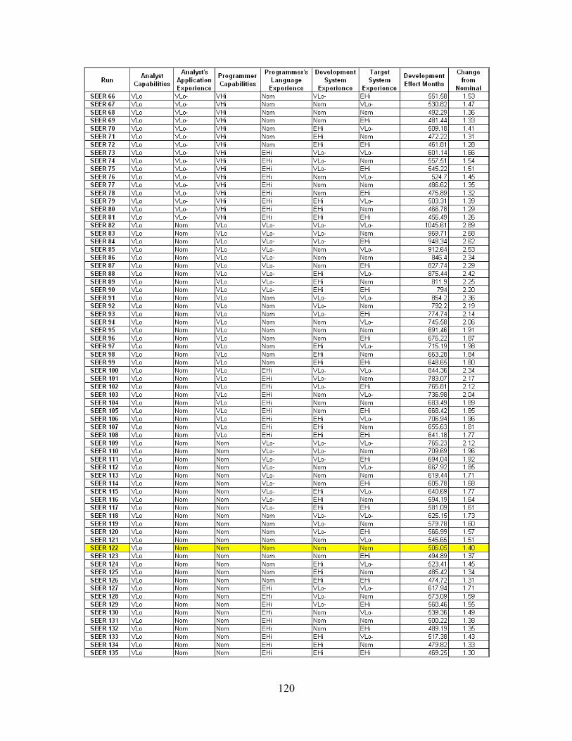
120

121
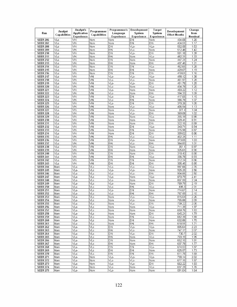
122

123

124

125

126

127

128

129

130
Appendix 9 SLIM Data Table

131
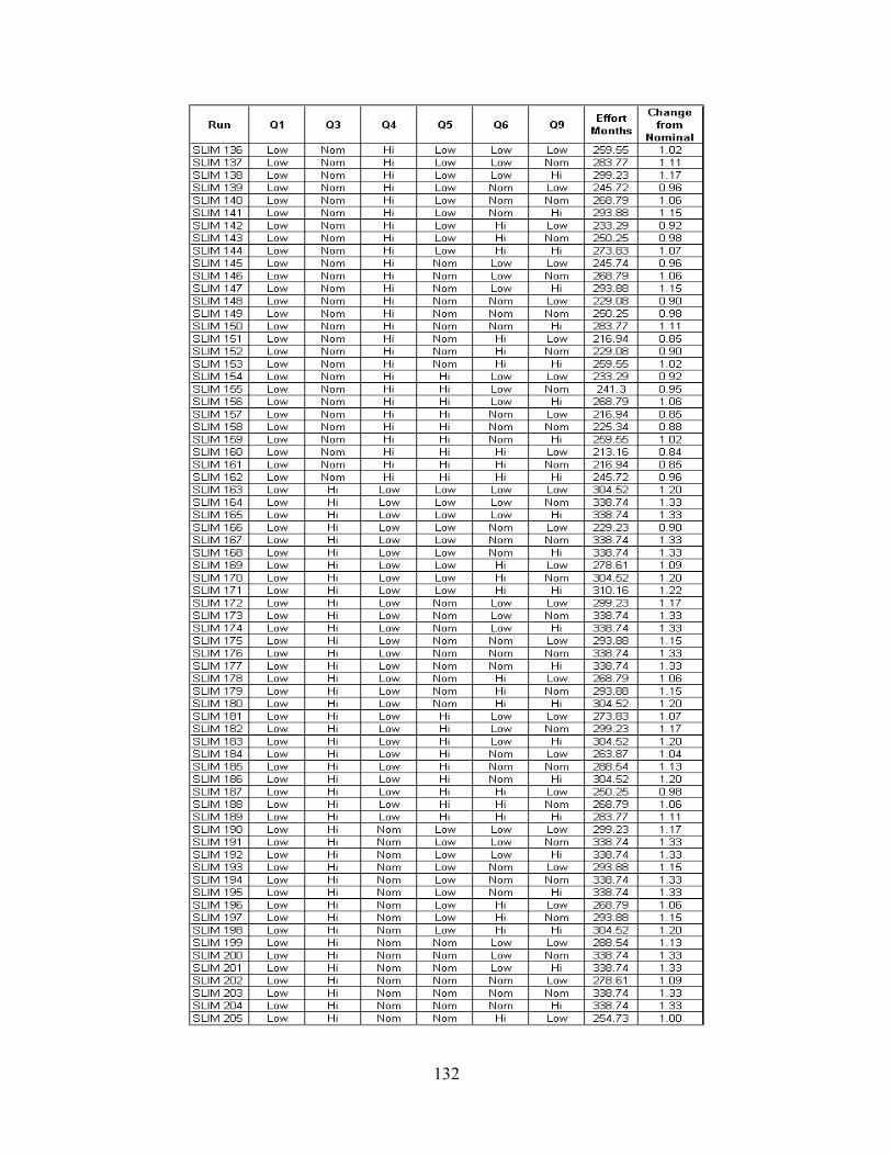
132

133

134

135

136

137
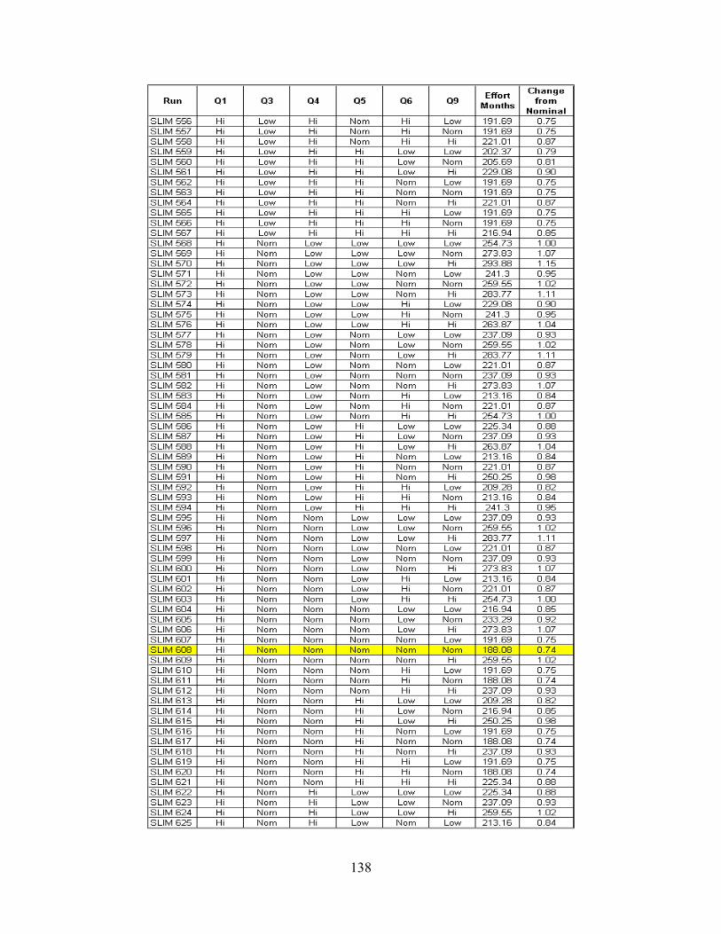
138
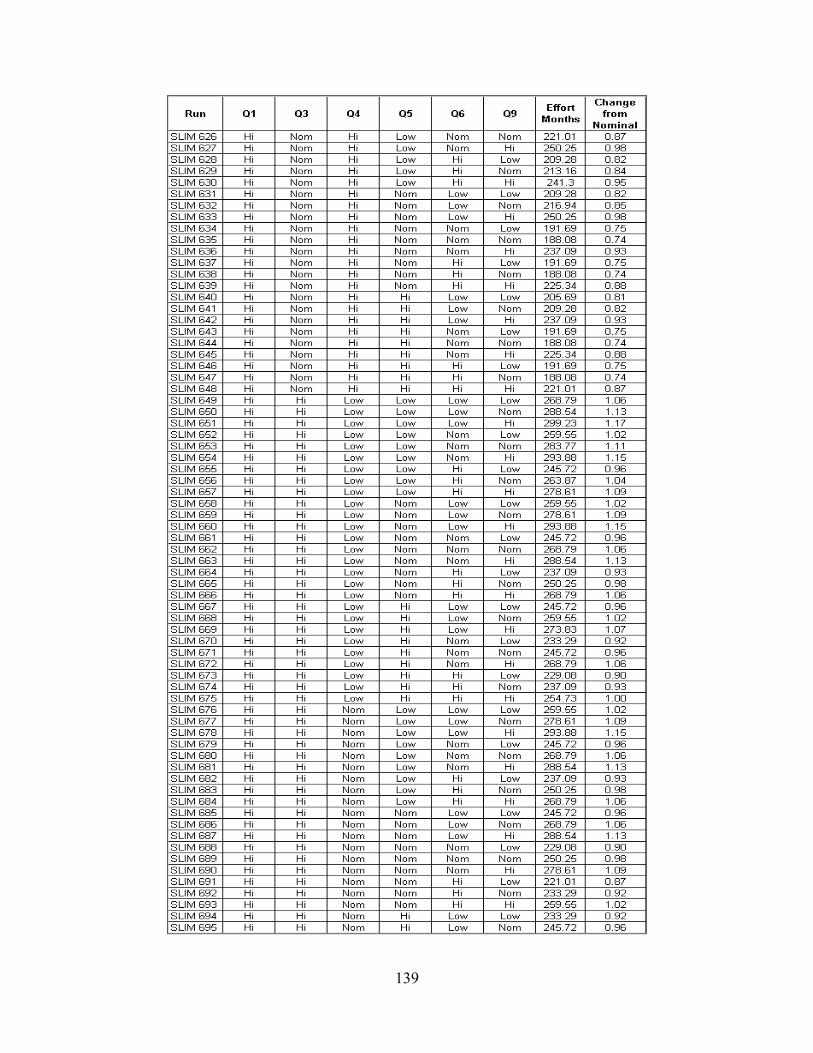
139

140

141
Appendix 10 PRICE S Data Table
142
Bibliography
1. Department of the Air Force. Parametric Estimating Handbook. http://www.ispa-cost.org/PEIWeb/newbook.htm 7 August 2002.
2. Hu, Qing, Robert T. Plant, and David B. Hertz, “Software Cost Estimation Using
Economic Production Models,” Journal of Management Information Systems, 15(1): 143-164 (Summer 1998).
3. Mannering, Virginia H., Gross Domestic Product: Fourth Quarter 2000, Bureau
of Economic Analysis, U.S. Dept. of Commerce, January 31, 2001. 4. Government Accounting Office. Embedded Computer Systems: Defense Does Not
Know How Much It Spends on Software. GAO/IMTEC-92-62BR. Washington: GPO, 1992.
5. Etter, Delores. “Acquisition Software Oversight,” Crosstalk: The Journal of
Defense Software Engineering, 12(8): 3 (August 1999).
6. Nelson, Mike, James Clark, Martha Ann Spurlock. “Curing the Software Requirements and Cost Estimating Blues,” Software Management & Cost Estimating, Vol: 54-60 (Nov-Dec 1999)
7. Government Accounting Office. Embedded Computer Systems: Significant
Software Problems on C-17 Must Be Addressed. GAO/IMTEC-92-48. Washington: GPO, 1992.
8. “Pentagon Warns It May Cancel Troubled C-17 Cargo Plane,” Congressional
Quarterly Weekly Report, 51(20): 1246-1247 (May 1993).
9. Brooks, Andrew. “Estimating Cost with Software,” Computing Canada, 24(34): 13-14 (Sept 1998).
10. Ferens, Dan V. “Software cost Estimation in the DoD environment,” American
Programmer, 9(7): 28-34 (July 1996).
11. Stutzke, Richard D. “Software Estimating Technology: A Survey,” Crosstalk: The Journal of Defense Software Engineering, 9(5): (May 1996).
12. Boehm, Barry W. Software Engineering Economics. New Jersey: Prentice Hall,
1981.
13. Sweet, Ann-Marie D. and others. Society of Cost Estimation and Analysis Glossary Excerpt from glossary. n. pag. http://www.sceaonline.net/ 7 August 2002.

143
14. Putnam, Lawrence H. Measures For Excellence: Reliable Software On Time,
Within Budget. Englewood Cliffs, New Jersey, 1992.
15. Department of the Air Force. The AFSC Cost Estimating Handbook Series. 1986.
16. Marban, Oscar, Juan J. Cuadrado, Antonio de Amescua, and Maria I. Sanchez. “The importance of rating level selection for input variables to determine accurate estimations in parametric mathematical models,” Journal of Cost Analysis and Management, (forthcoming).
17. Jones, Capers T. Estimating Software Costs. McGraw-Hill, 1998.
18. Boehm, Barry W. and K Sullivan, “Software economics: status and prospects,”
Information and Software Technology, 14:937-946 (Nov 1999).
19. Nicholas, John M. Project Management for Business and Technology: Principles and Practice. New Jersey: Prentice Hall, 2001.
20. Vose, David NMI. Risk Analysis: A Quantitative Guide. John Wiley & Sons,
2000.
21. Coleman, R. L. “Cost and Schedule Risk – CE V”Address to Air Force Institute of Technology students and faculty. Air Force Institute of Technology, Wright-Patterson AFB OH. 5 December 2002.
22. United States Congress. Information Management Technology Reform Act of
1996. Public Law No. 104-106, 104th Congress. Washington: GPO, 1996.
23. Boehm, Barry W. Software Cost Estimation with COCOMO II. Upper Saddle River, New Jersey, 2000.
24. SEER-SEMTM Software Estimation, Planning and Project Control. User’s
Manual Galorath Incorporated, March 2000 Update.
25. Quantitative Software Management, SLIM ESTIMATE For Windows, User’s Guide, 2001.
26. PRICE Systems, L.L.C., Your Guide to PRICE S, 1998.
27. Long, John NMI. Vice-President for Sales, Price Corporation, Long Beach CA.
Telephone interview. 25 July and 6 Nov 2002.
28. Montgomery, Douglas C. Design and Analysis of Experiments. John Wiley & Sons, 1991.

144
29. Vigder, Mark R and Anatol W. Kark. Software Cost Estimation and Control.
NRC No. 37116. Ottawa, Ontario, Canada: National Research Council of Canada, September 1994.
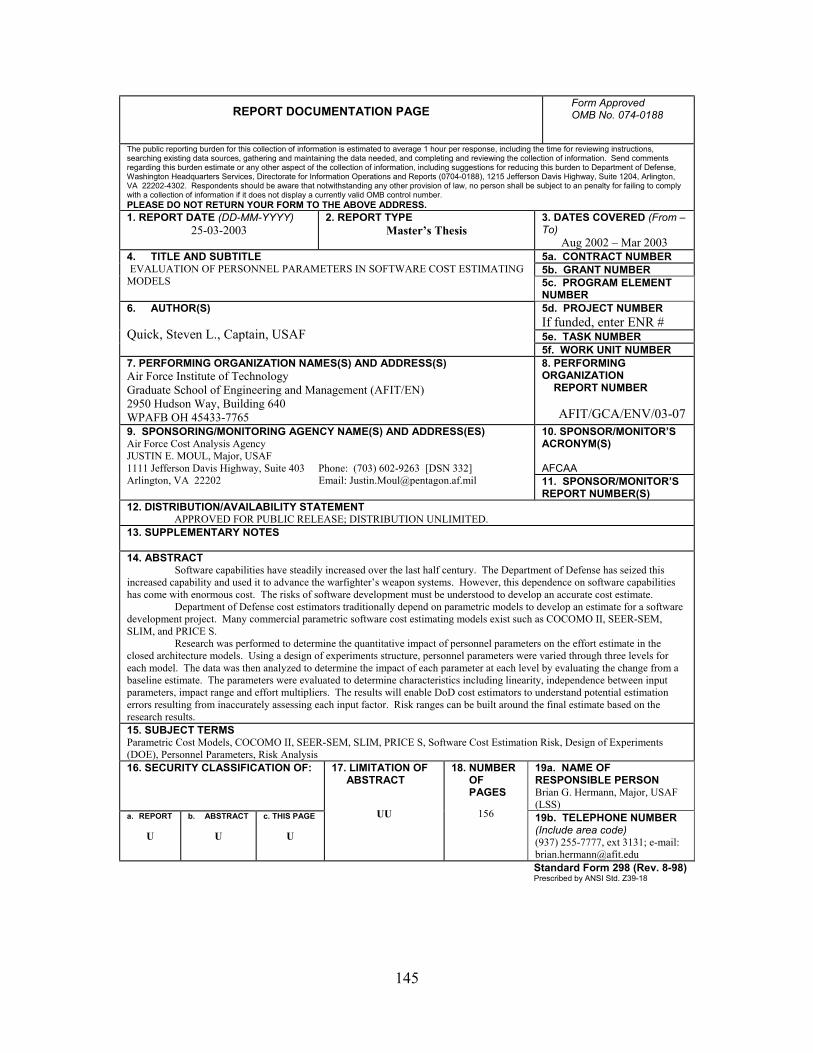
145
REPORT DOCUMENTATION PAGE Form Approved OMB No. 074-0188
The public reporting burden for this collection of information is estimated to average 1 hour per response, including the time for reviewing instructions, searching existing data sources, gathering and maintaining the data needed, and completing and reviewing the collection of information. Send comments regarding this burden estimate or any other aspect of the collection of information, including suggestions for reducing this burden to Department of Defense, Washington Headquarters Services, Directorate for Information Operations and Reports (0704-0188), 1215 Jefferson Davis Highway, Suite 1204, Arlington, VA 22202-4302. Respondents should be aware that notwithstanding any other provision of law, no person shall be subject to an penalty for failing to comply with a collection of information if it does not display a currently valid OMB control number. PLEASE DO NOT RETURN YOUR FORM TO THE ABOVE ADDRESS. 1. REPORT DATE (DD-MM-YYYY)
25-03-2003 2. REPORT TYPE
Master’s Thesis 3. DATES COVERED (From – To)
Aug 2002 – Mar 2003 5a. CONTRACT NUMBER 5b. GRANT NUMBER
4. TITLE AND SUBTITLE EVALUATION OF PERSONNEL PARAMETERS IN SOFTWARE COST ESTIMATING MODELS 5c. PROGRAM ELEMENT
NUMBER 5d. PROJECT NUMBER If funded, enter ENR # 5e. TASK NUMBER
6. AUTHOR(S) Quick, Steven L., Captain, USAF
5f. WORK UNIT NUMBER 7. PERFORMING ORGANIZATION NAMES(S) AND ADDRESS(S) Air Force Institute of Technology Graduate School of Engineering and Management (AFIT/EN) 2950 Hudson Way, Building 640 WPAFB OH 45433-7765
8. PERFORMING ORGANIZATION REPORT NUMBER AFIT/GCA/ENV/03-07 10. SPONSOR/MONITOR’S ACRONYM(S) AFCAA
9. SPONSORING/MONITORING AGENCY NAME(S) AND ADDRESS(ES) Air Force Cost Analysis Agency JUSTIN E. MOUL, Major, USAF 1111 Jefferson Davis Highway, Suite 403 Phone: (703) 602-9263 [DSN 332] Arlington, VA 22202 Email: [email protected] 11. SPONSOR/MONITOR’S
REPORT NUMBER(S) 12. DISTRIBUTION/AVAILABILITY STATEMENT
APPROVED FOR PUBLIC RELEASE; DISTRIBUTION UNLIMITED. 13. SUPPLEMENTARY NOTES 14. ABSTRACT Software capabilities have steadily increased over the last half century. The Department of Defense has seized this increased capability and used it to advance the warfighter’s weapon systems. However, this dependence on software capabilities has come with enormous cost. The risks of software development must be understood to develop an accurate cost estimate. Department of Defense cost estimators traditionally depend on parametric models to develop an estimate for a software development project. Many commercial parametric software cost estimating models exist such as COCOMO II, SEER-SEM, SLIM, and PRICE S. Research was performed to determine the quantitative impact of personnel parameters on the effort estimate in the closed architecture models. Using a design of experiments structure, personnel parameters were varied through three levels for each model. The data was then analyzed to determine the impact of each parameter at each level by evaluating the change from a baseline estimate. The parameters were evaluated to determine characteristics including linearity, independence between input parameters, impact range and effort multipliers. The results will enable DoD cost estimators to understand potential estimation errors resulting from inaccurately assessing each input factor. Risk ranges can be built around the final estimate based on the research results. 15. SUBJECT TERMS Parametric Cost Models, COCOMO II, SEER-SEM, SLIM, PRICE S, Software Cost Estimation Risk, Design of Experiments (DOE), Personnel Parameters, Risk Analysis 16. SECURITY CLASSIFICATION OF: 19a. NAME OF
RESPONSIBLE PERSON Brian G. Hermann, Major, USAF (LSS)
a. REPORT
U
b. ABSTRACT
U
c. THIS PAGE
U
17. LIMITATION OF ABSTRACT
UU
18. NUMBER OF PAGES
156 19b. TELEPHONE NUMBER (Include area code) (937) 255-7777, ext 3131; e-mail: [email protected]
Standard Form 298 (Rev. 8-98) Prescribed by ANSI Std. Z39-18