Embed Size (px)
Citation preview
The Texas Medical Center Library The Texas Medical Center Library
DigitalCommons@TMC DigitalCommons@TMC
The University of Texas MD Anderson Cancer Center UTHealth Graduate School of Biomedical Sciences Dissertations and Theses (Open Access)
The University of Texas MD Anderson Cancer Center UTHealth Graduate School of
Biomedical Sciences
8-2013
Evaluation of PRESAGE® dosimeters for brachytherapy sources Evaluation of PRESAGE® dosimeters for brachytherapy sources
and the 3D dosimetry and characterization of the new AgX100 and the 3D dosimetry and characterization of the new AgX100
125I seed model 125I seed model
Olivia Huang
Follow this and additional works at: https://digitalcommons.library.tmc.edu/utgsbs_dissertations
Part of the Medical Biophysics Commons
Recommended Citation Recommended Citation Huang, Olivia, "Evaluation of PRESAGE® dosimeters for brachytherapy sources and the 3D dosimetry and characterization of the new AgX100 125I seed model" (2013). The University of Texas MD Anderson Cancer Center UTHealth Graduate School of Biomedical Sciences Dissertations and Theses (Open Access). 393. https://digitalcommons.library.tmc.edu/utgsbs_dissertations/393
This Thesis (MS) is brought to you for free and open access by the The University of Texas MD Anderson Cancer Center UTHealth Graduate School of Biomedical Sciences at DigitalCommons@TMC. It has been accepted for inclusion in The University of Texas MD Anderson Cancer Center UTHealth Graduate School of Biomedical Sciences Dissertations and Theses (Open Access) by an authorized administrator of DigitalCommons@TMC. For more information, please contact [email protected].
The University of Texas-Houston M.D. Anderson Cancer Center
Graduate School of Biomedical Sciences
Evaluation of PRESAGE® dosimeters for brachytherapy
sources and the 3D dosimetry and characterization
of the new AgX100 125
I seed model
A
THESIS
Presented to the faculty of
The University of Texas
M. D. Anderson Cancer Center
Graduate School of Biomedical Sciences
In Partial Fulfillment
Of the Requirements
For the Degree of
SPECIALIZED MASTER OF SCIENCE
By
Olivia Huang, B.S.
Houston, Texas
August 2013

Acknowledgements
First and foremost, I would like to acknowledge my advisor, Dr. Geoffrey Ibbott.
Thank you for your patience, guidance, and encouragement throughout this project and these
past two years of graduate school. I would also like to thank the members of my committee -
Dr. David Followill, Dr. Kent Gifford, Dr. Shouhou Zhou, and Dr. Ramesh Tailor – for their
expert advice and time invested in this project. I would like to also acknowledge Dr. John
Adamovics for manufacturing the several batches of dosimeters used in this project.
Furthermore, I would like to thank Ryan Grant, M.S. for teaching me how to use the
PRESAGE®/DMOS system and for being the PRESAGE
® guru of our lab group. To the rest
of our lab group- Slade Klawikowski, Ph.D., Mitchell Carroll, M.S., and Yvonne Roed-
thank you for all of their help and suggestions, especially during the troubleshooting phase
of this project. I would also like to thank Theragenics Corporation for sending us a higher
activity AgX100 seed for this project.
The staff members at the ADCL at M.D. Anderson Cancer Center - Stephanie
Lampe, Charles Darcy-Clarke, and Regina Garcia – were amazingly kind and patient in
helping me obtain sources and letting me into the LDR Brachytherapy room doors for each
and every irradiation. I would also like to thank my fellow classmates at the RPC,
particularly James Neihart, Christopher Pham, and Elizabeth McKenzie, for their support,
encouragement, and their sense of humor, which helped keep me sane during stressful times.
iii

Dedication
To Shuja-
Thank you for your patience and encouragement. These past two years in graduate school
would have been terrifying without you.
To my parents-
Thank you both for always believing in me and for giving me all the tools in life to succeed.
iv
Evaluation of PRESAGE® dosimeters for brachytherapy sources and
the 3D dosimetry and characterization of the new AgX100 125I seed model
Publication No. _________
Olivia Huang, B.S.
Supervisory Professor: Geoffrey S. Ibbott, Ph.D.
With continuous new improvements in brachytherapy source designs and techniques,
method of 3D dosimetry for treatment dose verifications would better ensure accurate
patient radiotherapy treatment. This study was aimed to first evaluate the 3D dose
distributions of the low-dose rate (LDR) Amersham 6711 OncoseedTM
using PRESAGE®
dosimeters to establish PRESAGE® as a suitable brachytherapy dosimeter. The new
AgX100 125
I seed model (Theragenics Corporation) was then characterized using
PRESAGE® following the TG-43 protocol.
PRESAGE® dosimeters are solid, polyurethane-based, 3D dosimeters doped with
radiochromic leuco dyes that produce a linear optical density response to radiation dose. For
this project, the radiochromic response in PRESAGE® was captured using optical-CT
scanning (632 nm) and the final 3D dose matrix was reconstructed using the MATLAB
software. An Amersham 6711 seed with an air-kerma strength of approximately 9 U was
used to irradiate two dosimeters to 2 Gy and 11 Gy at 1 cm to evaluate dose rates in the r=1
cm to r=5 cm region. The dosimetry parameters were compared to the values published in
the updated AAPM Report No. 51 (TG-43U1). An AgX100 seed with an air-kerma strength
v
of about 6 U was used to irradiate two dosimeters to 3.6 Gy and 12.5 Gy at 1 cm. The
dosimetry parameters for the AgX100 were compared to the values measured from previous
Monte-Carlo and experimental studies[1,2].
In general, the measured dose rate constant, anisotropy function, and radial dose
function for the Amersham 6711 showed agreements better than 5% compared to consensus
values in the r=1 to r=3 cm region. The dose rates and radial dose functions measured for the
AgX100 agreed with the MCNPX and TLD-measured values within 3% in the r=1 to r=3
cm region. The measured anisotropy function in PRESAGE® showed relative differences of
up to 9% with the MCNPX calculated values. It was determined that post-irradiation optical
density change over several days was non-linear in different dose regions, and therefore the
dose values in the r=4 to r=5 cm regions had higher uncertainty due to this effect. This study
demonstrated that within the radial distance of 3 cm, brachytherapy dosimetry in
PRESAGE® can be accurate within 5% as long as irradiation times are within 48 hours.
vi

Table of Contents
Signature Page ................................................................................................................. i
Title Page ........................................................................................................................ ii
Acknowledgements ........................................................................................................ iii
Dedications .................................................................................................................... iv
Abstract ........................................................................................................................... v
Table of Contents .......................................................................................................... vii
List of Figures ................................................................................................................. x
List of Tables ................................................................................................................ xii
Chapter 1- Introduction ............................................................................................... 1
1.1 Statement of Problem .......................................................................................... 1
1.1.1 General Problem Area ................................................................................. 1
1.1.2 Specific Problem Area ................................................................................. 2
1.2 Background .......................................................................................................... 2
1.2.1 Brachytherapy .............................................................................................. 2
1.2.1.1 Amersham 6711 .............................................................................. 6
1.2.1.2 AgX100........................................................................................... 7
1.2.2 History of Gel Dosimetry ............................................................................ 9
1.2.3 PRESAGE® Dosimeters ............................................................................ 12
1.2.3.1 Characteristics of PRESAGE®
..................................................... 12
1.2.3.2 Optical-CT Imaging ...................................................................... 15
1.2.3.2.1 The OCTOPUS ................................................................ 15
1.2.3.2.2 Duke Mid-sized Optical-CT Scanner .............................. 16
1.2.3.3. Drawbacks of PRESAGE®
......................................................... 18
1.2.3.4 Previous work with PRESAGE®
................................................. 19
vii
1.3 Hypothesis and Specific Aim ............................................................................ 21
Chapter 2- Materials and Methods ........................................................................... 21
2.1 Dosimeter Design .............................................................................................. 21
2.2 Treatment Set-up and Delivery .......................................................................... 27
2.2.1 Pre-Irradiation ............................................................................................ 27
2.2.2 Dose Calibration ........................................................................................ 28
2.2.3 Treatment Delivery .................................................................................... 30
2.3 Imaging and Analysis ........................................................................................ 33
2.3.1 Optical-CT Imaging ................................................................................... 33
2.3.2 Data Acquisition in CERR......................................................................... 34
2.4 TG-43 Formalism .............................................................................................. 37
2.4.1 Air-kerma Strength .................................................................................... 39
2.4.2 Dose Rate ................................................................................................... 40
2.4.3 Dose Rate Constant.................................................................................... 42
2.4.4. Geometry Function ................................................................................... 43
2.4.5 Anisotropy Function .................................................................................. 44
2.4.6 Radial Dose Function ................................................................................ 46
Chapter 3- Results and Discussion for the Amersham 6711 ................................... 48
3.1 Dose Rate ........................................................................................................... 48
3.2 Dose Rate Constant............................................................................................ 51
3.3 Anisotropy Function .......................................................................................... 52
3.4 Radial Dose Function ........................................................................................ 56
Chapter 4- Results and Discussion for the AgX100 ................................................. 58
4.1 General Discussion of Results ........................................................................... 58
4.2 Dose Rate .......................................................................................................... 60
viii

4.3 Dose Rate Constant............................................................................................ 61
4.4 Anisotropy Function .......................................................................................... 62
4.5 Radial Dose Function ........................................................................................ 66
Chapter 5- Discussion of the over-response in PRESAGE® at low doses .............. 68
5.1 Post-irradiation OD change over time ............................................................... 68
5.2 Method of correction ......................................................................................... 75
Chapter 6- Uncertainty Analysis ............................................................................... 78
6.1 Uncertainty in the Dose Rate Constant .............................................................. 78
6.2 Uncertainty in Anisotropy Function ................................................................. 80
6.3 Uncertainty in Radial Dose Function ................................................................ 80
Chapter 7- Conclusion ................................................................................................ 80
Appendix A .................................................................................................................. 83
Appendix B .................................................................................................................. 86
References .................................................................................................................... 97
Vita ............................................................................................................................. 103
ix
List of Figures
Figure 1. Amersham 6711 OncoSeed model design[14] .................................................... 6
Figure 2. Dimensions of the Theragenics AgX100 ............................................................ 8
Figure 3 Example of an irradiated PRESAGE® dosimeter ............................................... 12
Figure 4. Example of a Calibration Curve for PRESAGE®
............................................. 14
Figure 5. Diagram illustrating main components of the DMOS ....................................... 17
Figure 6. The o-MeO-LMG PRESAGE® formulation ..................................................... 22
Figure 7. PRESAGE® dosiemter with 0.4 cm diameter channel ...................................... 24
Figure 8. PRESAGE® dosimeter with 1.5 cm diameter channel ...................................... 25
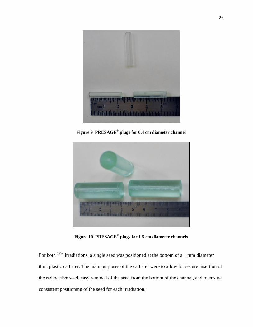
Figure 9 PRESAGE® plugs for 0.4 cm diameter channel ................................................ 26
Figure 10 PRESAGE® plugs for 1.5 cm diameter channels ............................................ 26
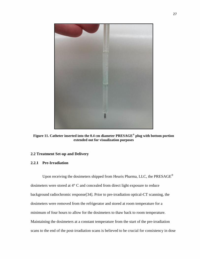
Figure 11. Catheter inserted into the 0.4 cm diameter PRESAGE®
plug ......................... 27
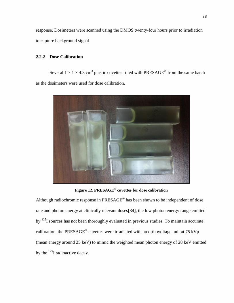
Figure 12. PRESAGE® cuvettes for dose calibration ....................................................... 28
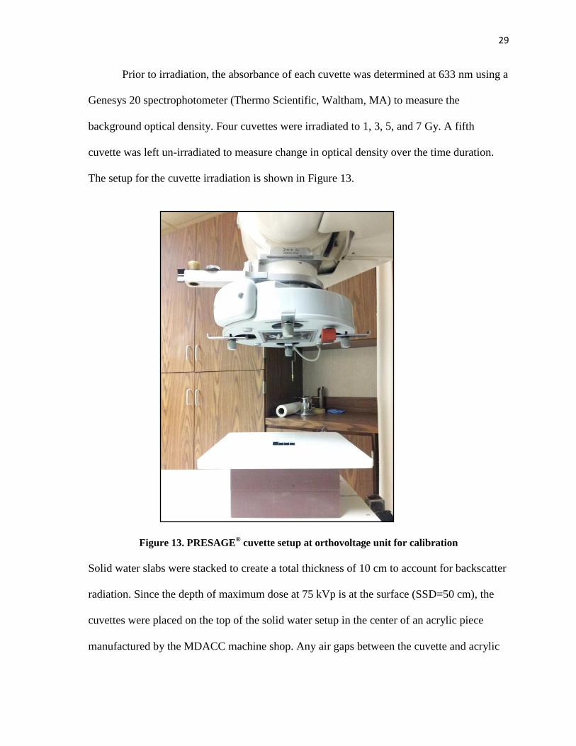
Figure 13. PRESAGE® cuvette setup at orthovoltage unit for calibration ....................... 29
Figure 14. Dosimeter (shielded from light) positioned in rice tank for backscatter ......... 31
Figure 15. Dosimeter with plug, catheter, and 6711 seed ................................................. 32
Figure 16. Screen capture of the Duke 3D Dosimetry Lab interface for reconstruction .. 34
Figure 17. Sagittal, Transverse and Coronal views of reconstructed dose cube in CERR 36
Figure 18. Dose line profile generated in CERR .............................................................. 36
Figure 19. Coordinate system for brachytherapy dosimetry as defined from TG-43 ....... 37
Figure 20. Transverse bisecting plane determined in CERR ............................................ 39
Figure 21. Diagram illustrating the 12 measurement points in PRESAGE® for each point
of interest for dose rate, anisotropy function, and radial dose function calculations........ 41
x
Figure 22. Amersham 6711: Dose Rate Comparison ....................................................... 49
Figure 23. Isodose lines in a large dosimeter displayed in CERR. ................................... 50
Figure 24. AgX100 Anisotropy functions for r = 1 cm. ................................................... 54
Figure 25. AgX100 Anisotropy functions for r =2 cm. .................................................... 54
Figure 26. AgX100 Anisotropy functions for r = 3 cm. ................................................... 55
Figure 27. AgX100 Anisotropy functions for r = 4 cm. ................................................... 55
Figure 28. AgX100 Anisotropy functions for r = 5 cm. ................................................... 56
Figure 29. Comparison of AgX100 radial dose functions. ............................................... 58
Figure 30. AgX100 Dose Rate Comparison. .................................................................... 61
Figure 31. AgX100 Anisotropy Function at r = 1 cm. ...................................................... 65
Figure 32. AgX100 Anisotropy Function at r = 2 cm. ...................................................... 65
Figure 33. AgX100 Anisotropy Function at r = 3 cm. ...................................................... 66
Figure 34. AgX100: Radial Dose Function Comparison. ................................................. 67
Figure 35. Calibration curve demonstrating linearity in dose response ............................ 69
Figure 36. OD change over time for PRESAGE® at 0 Gy .............................................. 70
Figure 37. OD change over time for PRESAGE® at 1 Gy .............................................. 71
Figure 38. OD change over time for PRESAGE® at 3 Gy .............................................. 71
Figure 39. OD change over time for PRESAGE® at 5 Gy .............................................. 72
Figure 40. OD change over time for PRESAGE® at 7 Gy .............................................. 72
Figure 41. Isodose lines of AgX100-irradiated large channel dosimeter ......................... 75
xi

List of Tables
Table 1: Categories of brachytherapy as defined in ICRU Report 38[13] ......................... 4
Table 2: List of radionuclides and their characteristics[14,15,16]...................................... 5
Table 3. Doses calculated for 20 cGy at 5 cm .................................................................. 23
Table 4. Dose rate using 2D formalism for the Amersham 6711 ..................................... 40
Table 5. Dose rates using 2D formalism for the AgX100 ................................................ 40
Table 6. Dose rate constants for both 125
I seed models..................................................... 43
Table 7. Geometry Factors for L=3 mm ........................................................................... 44
Table 8. Geometry Factors for L=3.5 mm ........................................................................ 44
Table 9. Anisotropy Function Table for Amersham 6711 ................................................ 45
Table 10. Radial Dose Functions for the Amersham 6711 ............................................... 47
Table 11. Amersham 6711: Dose Rate Comparison ......................................................... 48
Table 12. Amersham 6711: Comparison of the doses delivered ...................................... 50
Table 13. Amersham 6711: Comparison of the dose rate constant .................................. 51
Table 14. Amersham 6711: Anisotropy Functions measured in PRESAGE®
.................. 52
Table 15. Amersham 6711 Anisotropy Functions: Relative Differences (%) .................. 53
Table 16. Amersham 6711: Radial Dose Function Comparison ...................................... 57
Table 17. Dose Comparison in 0.4 cm channel dosimeter ............................................... 58
Table 18. Dose Comparison in 1.5 cm channel dosimeter ............................................... 59
Table 19. AgX100: Dose Rate Comparison ..................................................................... 60
Table 20. Dose Rate constants of the AgX100 ................................................................. 62
Table 21. Dose Rate Constant Comparison ...................................................................... 62
Table 22. AgX100: Anisotropy Function measured in PRESAGE®
................................ 63
xii
Table 23. AgX100: TLD-measured Anisotropy Functions[2] .......................................... 63
Table 24. AgX100: Monte-Carlo calculated Anisotropy Functions[1] ............................ 64
Table 27. AgX100- Radial Dose Function Comparison ................................................... 66
Table 28. OD change at several time points post-irradiation ............................................ 69
Table 29. OD change at several time points post-irradiation (continued) ........................ 69
Table 30. Table describing dose deposited on Day 1 at r=4cm and the calculated OD-
Ratio .................................................................................................................................. 76
Table 31. “Corrected” doses at each radial distance for the 6711-irradiated dosimeter ... 77
Table 32. Uncertainty in PRESAGE® measurements of the dose rate constant ............... 79
xiii
1
1 Introduction
1.1 Statement of Problem
1.1.1 General Problem Area
Radiation therapy has advanced dramatically in complexity since the first paper on
the concept of Intensity Modulated Radiation Therapy (IMRT) was published in 1994[3].
Cutting-edge technology allows for radiotherapy methods to continuously improve
conformality to the target volume, which can result in higher radiation doses administered to
the tumor site to eradicate cancer while keeping normal tissue toxicity low. However, with
such rapid advances it is imperative to balance the complex radiation therapy techniques
with suitable quality assurance (QA) methods to ensure accurate clinical patient treatment
and patient safety.
Currently, three dimensional (3D) IMRT dosimetric verification for commissioning
and patient-specific QA is generally performed with the combination of absolute point dose
measurements using a calibrated ion chamber and a two dimensional (2D) planar dosimetric
analysis with radiochromic film or a diode array[4]. These methods provide a dosimetric
check of volumetric sampling. However, the complexity of multiple beams with high doses
and steep dose gradients make it very difficult to accurately and comprehensively verify the
actual 3D dose distributions. With radiation doses as high as 40 Gy per treatment fraction in
stereotactic radiosurgery, it is clear that an accurate method of comprehensive 3D dose
verification through actual measurements is the next step in QA techniques to keep up with
radiotherapy advancements and to ensure accurate patient treatment.
2
1.1.2 Specific Problem Area
More specifically among the variety of radiation therapy techniques, an accurate
method of 3D dosimetry in brachytherapy is needed. Both high dose rate (HDR) and low
dose rate (LDR) brachytherapy are commonly used modalities in radiation oncology centers
worldwide. Methods in positioning sources in a designed formation to shape the dose
distribution are advancing in brachytherapy, such as the COMS eye plaque for LDR
treatment of choroidal melanoma[5] or various HDR applicator devices like the SAVI
device for accelerated partial breast irradiation[6]. For the COMS eye plaque in particular,
only a select few have carefully evaluated the COMS eye plaque dosimetry[7] and
biological effective dose[8] through Monte Carlo simulations. 3D dosimetric verifications
through experimental methods have yet to be published.
The success of LDR multi-source irradiations relies heavily on the rapid dose fall-off
beyond the tumor volume, and typically doses as high as 85 Gy (typical eye plaque
prescription dose) are delivered to the target. With high doses delivered to small volumes, a
reliable QA method of 3D dosimetry for these brachytherapy devices is important for patient
treatment. Additionally, a method of 3D dosimetry for LDR sources would greatly simplify
the experimental methods in obtaining data for dosimetric characterization of new
radioactive seed models.
1.2 Background
1.2.1 Brachytherapy
Brachytherapy is a technique in radiation therapy where one or several sealed
radioactive sources are placed in close proximity to the tumor or treatment site using

3
interstitial, intracavitary, intravascular, or surface applicator methods. From its Greek
derivation “brachy,” brachytherapy literally means ‘short range therapy,’ which refers to the
short therapeutic range of the emitted radiation from the decay of the radioisotope.
Brachytherapy seeds are commonly used in oncology centers worldwide for radiation
therapy, typically in prostate, cervical, breast, and eye plaque brachytherapy treatments.
Not long after Marie Curie’s discovery of Radium-226 in 1898, the concept of
inserting a radium-filled tube into a tumor for clinical treatment of cancer followed in 1901
by Pierre Curie[9]. By 1904, small amounts of radium encapsulated in glass tubes were used
clinically through applications on the skin surface and intratumoral implantations[9].
However, high costs for radium and difficulties in establishing an effective treatment
method resulted in the decline of brachytherapy use until the discovery of the method to
create artificial radionuclides in 1934, by Irene and Frederic Joliot-Curie[10]. Man-made
radionuclides allowed for more control over the amount of administered radioactivity and
the sizes and shapes of the encapsulated radioactivity. More options in the emitted energy
range and half-life also became available and the start of a modern age of brachytherapy
began. Remote afterloading technology, which greatly reduced personnel exposure to high
activity sources, was introduced by Walstam and Henschke et al in the early 1960s,
ultimately paving the way for HDR brachytherapy[11].
The main advantage of brachytherapy is the ability to manually position radioactive
sources within or near the cancer site for exceptionally high doses to be delivered to the
tumor volume. Since radiation dose falls off rapidly with distance according to the inverse
square law, only the immediate region surrounding the treatment site is irradiated, while
most normal tissue, particularly organs at risk, is spared of dose. Additionally, the dose rate
4
is much lower in brachytherapy, especially in LDR brachytherapy, compared to external
beam radiation therapy. A lower dose rate renders a higher radiobiological advantage since
longer periods of time between damaging “hits” allows for increased probability of repair of
sublethally damaged DNA[9]. Furthermore, HDR and LDR brachytherapy typically have
relatively short treatment times of less than 55 days, which advantageously hinders tumor
repopulation[12].
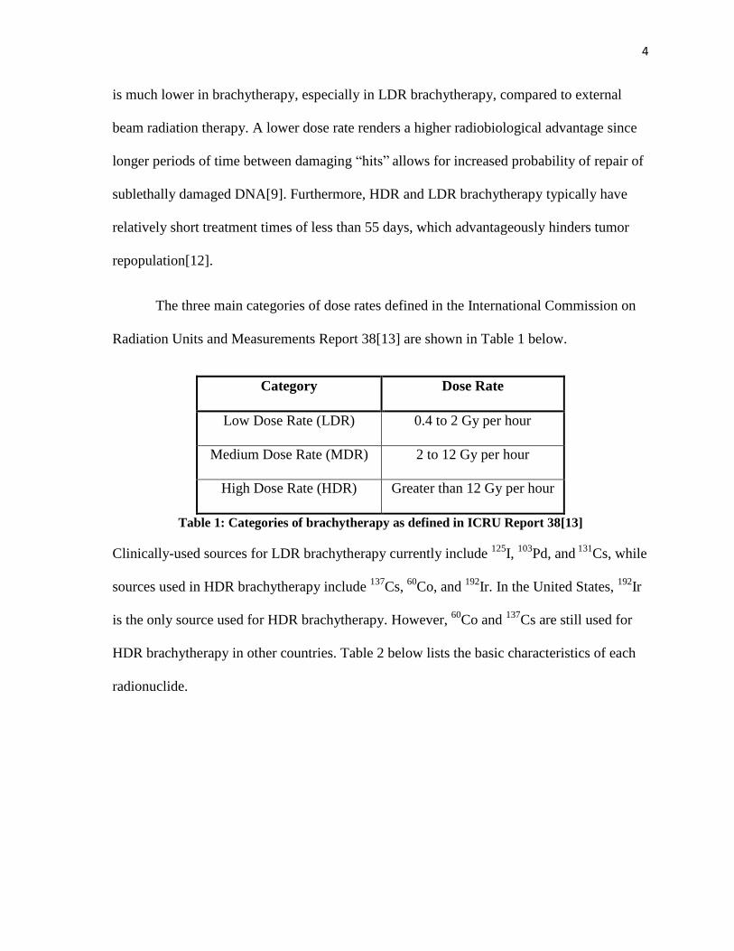
The three main categories of dose rates defined in the International Commission on
Radiation Units and Measurements Report 38[13] are shown in Table 1 below.
Category Dose Rate
Low Dose Rate (LDR) 0.4 to 2 Gy per hour
Medium Dose Rate (MDR) 2 to 12 Gy per hour
High Dose Rate (HDR) Greater than 12 Gy per hour
Table 1: Categories of brachytherapy as defined in ICRU Report 38[13]
Clinically-used sources for LDR brachytherapy currently include 125
I, 103
Pd, and 131
Cs, while
sources used in HDR brachytherapy include 137
Cs, 60
Co, and 192
Ir. In the United States, 192
Ir
is the only source used for HDR brachytherapy. However, 60
Co and 137
Cs are still used for
HDR brachytherapy in other countries. Table 2 below lists the basic characteristics of each
radionuclide.
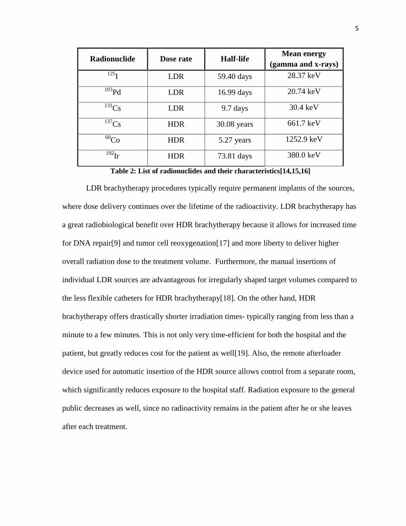
5
Radionuclide Dose rate Half-life Mean energy
(gamma and x-rays) 125
I LDR 59.40 days 28.37 keV
103Pd LDR 16.99 days 20.74 keV
131Cs LDR 9.7 days 30.4 keV
137Cs HDR 30.08 years 661.7 keV
60Co HDR 5.27 years 1252.9 keV
192Ir HDR 73.81 days 380.0 keV
Table 2: List of radionuclides and their characteristics[14,15,16]
LDR brachytherapy procedures typically require permanent implants of the sources,
where dose delivery continues over the lifetime of the radioactivity. LDR brachytherapy has
a great radiobiological benefit over HDR brachytherapy because it allows for increased time
for DNA repair[9] and tumor cell reoxygenation[17] and more liberty to deliver higher
overall radiation dose to the treatment volume. Furthermore, the manual insertions of
individual LDR sources are advantageous for irregularly shaped target volumes compared to
the less flexible catheters for HDR brachytherapy[18]. On the other hand, HDR
brachytherapy offers drastically shorter irradiation times- typically ranging from less than a
minute to a few minutes. This is not only very time-efficient for both the hospital and the
patient, but greatly reduces cost for the patient as well[19]. Also, the remote afterloader
device used for automatic insertion of the HDR source allows control from a separate room,
which significantly reduces exposure to the hospital staff. Radiation exposure to the general
public decreases as well, since no radioactivity remains in the patient after he or she leaves
after each treatment.
6
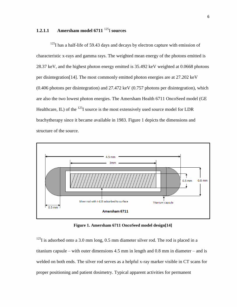
1.2.1.1 Amersham model 6711 125
I sources
125I has a half-life of 59.43 days and decays by electron capture with emission of
characteristic x-rays and gamma rays. The weighted mean energy of the photons emitted is
28.37 keV, and the highest photon energy emitted is 35.492 keV weighted at 0.0668 photons
per disintegration[14]. The most commonly emitted photon energies are at 27.202 keV
(0.406 photons per disintegration) and 27.472 keV (0.757 photons per disintegration), which
are also the two lowest photon energies. The Amersham Health 6711 OncoSeed model (GE
Healthcare, IL) of the 125
I source is the most extensively used source model for LDR
brachytherapy since it became available in 1983. Figure 1 depicts the dimensions and
structure of the source.
Figure 1. Amersham 6711 OncoSeed model design[14]
125I is adsorbed onto a 3.0 mm long, 0.5 mm diameter silver rod. The rod is placed in a
titanium capsule – with outer dimensions 4.5 mm in length and 0.8 mm in diameter – and is
welded on both ends. The silver rod serves as a helpful x-ray marker visible in CT scans for
proper positioning and patient dosimetry. Typical apparent activities for permanent
7
interstitial implants with 125
I seeds are within the range of 0.19 to 1.016 mCi or 0.243 to
1.291 U[20].
The Amersham 6711 seed model has been thoroughly evaluated by numerous
researchers in the past few decades. The American Association for Physicists in Medicine
(AAPM) published an Update of the Task Group No. 43 Report (TG-43U1) for
brachytherapy dose calculations, which includes the general consensus dosimetry
parameters of the Amersham 6711 widely followed for clinical use today[14]. The
dosimetry parameters include the dose-rate constant, geometry function, radial dose
function, and anisotropy function. These parameters were established and published in the
TG-43U1 report to serve as the recommended standards for accurate brachytherapy
dosimetry in the United States and internationally. Each parameter depends on the specific
design of the radioactive source, and the consensus values were agreed upon by the
members of the Brachytherapy Subcommittee through careful evaluation of the strengths
and limitations of the techniques used for dosimetric characterization.
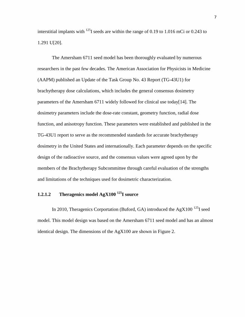
1.2.1.2 Theragenics model AgX100 125
I source
In 2010, Theragenics Corportation (Buford, GA) introduced the AgX100 125
I seed
model. This model design was based on the Amersham 6711 seed model and has an almost
identical design. The dimensions of the AgX100 are shown in Figure 2.
8
Figure 2. Dimensions of the Theragenics AgX100
Similar to the 6711 model, the AgX100 125
I source is encapsulated in a titanium capsule
welded on both ends. The seed has an outer length of 4.5 mm and a diameter of 0.8 mm. The
main difference lies in the dimensions of the 125
I covered silver rod. The active length of the
AgX100 is approximately 3.5 mm with a diameter of 0.59 mm, which is slightly larger than
the active dimensions of the Amersham 6711 source. The AgX100 seed still remains to be a
new source model to radiation oncology clinics and little work has been invested in the
evaluation of this seed.
The AAPM TG-43U1 recommends “independent and redundant dosimetric
characterizations” for any new seed models manufactured for clinical use[14]. Two main
studies have evaluated and characterized the AgX100 seed model following TG-43
formalism. In 2012, Mourtada et al determined the dosimetric parameters of the AgX100
through Monte Carlo calculations[1]. Comparing the dose distributions surrounding the
AgX100 in liquid water versus the 6711 model, the authors determined that the TG-43U1
dosimetric parameters for the two models were very similar except in the regions closest in
proximity to the seed. These findings are expected since the active length of the new seed
9
model is much longer than the one in the 6711 model. Thus, Mourtada et al recommended
separate TG-43U1 parameters to be established to account for these geometrical differences.
Chen et al also determined the dosimetric parameters of the AgX100 model in 2012[2]. The
authors used a germanium spectrometer to determine the photon energies emitted by the
seed and LiF thermoluminescent dosimeters (TLDs) in a solid water phantom to determine
the dosimetric parameters. The photon energy spectrum emitted from the AgX100 was
almost indistinguishable from the spectrum published in TG-43U1 for the Amersham 6711.
In comparison to the Monte Carlo-derived values by Mourtada et al, the measured dose rate
constant, radial dose functions, and anisotropy functions were generally within 5%. The
anisotropy functions for Ѳ<10⁰, however, showed a rather large disagreement of up to
20.5% compared to the Monte Carlo-calculated anisotropy functions. The authors believe
that the discrepancies may be due to intrinsic uncertainties in TLDs and the confined area of
TLDs for dose measurements. Following the recommendations of these authors and TG-43,
further evaluation of the dosimetric parameters of the AgX100 seed model is necessary for
accurate dosimetry and optimal clinical use for patients.
1.2.2 History of Gel Dosimetry
Gel dosimetry has continuously been a topic of interest in medical physics since
Andrews et al first investigated radiation depth doses in chloral hydrate diffused agar gel
with spectrophotometry and pH probes in 1957[21]. The appealing offer of a direct method
of capturing high spatial resolution 3D dose distributions over the complex and
computationally intensive methods in calculating and verifying dose distributions has
advanced several important accomplishments in the last few decades.
10
In 1984, Gore et al. presented the first method of imaging radiation dose distributions
using magnetic resonance imaging (MRI) in Fricke gels, a ferrous sulphate chemical
dosimeter (developed by Fricke and Morse in 1927) that undergoes an oxidative conversion
from ferrous ion (Fe2+
) to ferric ion (Fe3+
) when exposed to radiation. It was demonstrated
that the relaxation time of the protons in ferric ions was longer than ferrous ions, and thus a
higher resulting concentration of ferric ions rendered a longer total relaxation rate, which
allowed for dose estimations in Fricke gels[22]. Unfortunately, unreliable spatial accuracy
due to the diffusion of ions in Fricke gel[23] resulted in difficulties yet to be resolved
despite various attempts with chelating agents[24] and gelling agents to minimize the
diffusion.
The focus of gel dosimetry then turned to polymer gels. In 1992, Maryanki et al.
developed an agarose-based polymer gel called BANANA, which is an acronym for the
chemical components: Bis, Acrylamide, Nitrous oxide, ANd Agarose. This gel undergoes
radiation-induced polymerization and cross-linking of polymer chains which produces a
stable dose response over time- a great advantage over the ion diffusion problem in Fricke
gel[25]. Changes in proton relaxation rates in the polymers due to the polymerization and
cross-linking still allowed for the MRI imaging capability for dose analysis. In 1993,
Maryanski et al improved the polymer gel by using gelatin instead of agarose and thus
giving it the new name, BANG (acronym for Bis, Acrylamide, Nitrogen and aqueous
Gelatin)[26].The relaxation rate of water in gelatin gel is substantially lower than in agarose
gels, therefore the background signal of the polymer gel is minimized and the dynamic range
of the gel dosimeter increased[27]. A succession of further improvements in BANG gel
11
formulations led to several investigations of the clinical applications of polymer gels
demonstrating great potential for clinical use.
Gore et al[28] and Maryanski et al[29] presented in 1996 the method of optical
computed tomography (optical-CT) imaging as a more efficient and sensitive technique
compared to MRI for imaging gel dosimeters. Oldham et al advanced the optical-CT
technique in the 2003-2004[30,31], eventually leading to the design and manufacture of the
optical-CT scanner used in this project.
Although polymer gel dosimetry has high potential as a 3D dosimeter, several
drawbacks limit the practical clinical use of these gels. The greatest disadvantage of polymer
gels is the high sensitivity to atmospheric oxygen. Oxygen acts as a free-radical inhibitor in
polymer gels and results in the inhibition of polymerization response to radiation[26]. The
polymer gels need to be synthesized and stored in an oxygen-free environment, which
presents complications in the manufacturing process and clinical-use. Additionally, radiation
dose response in polymer gel relies on light scattering effects that generate a change in the
optical density. The scattered light photons have been shown to cause scatter artifacts within
the gel which affect the accuracy of the dose response. The external container required to
hold the gel also introduces large edge artifacts with optical-CT due to the differences in
refractive indices of the container, gel, and the matching fluid[32]. Thus, PRESAGE®
dosimeters were introduced in 2003 by J. Adamovics and M. J. Maryanski[33].
12
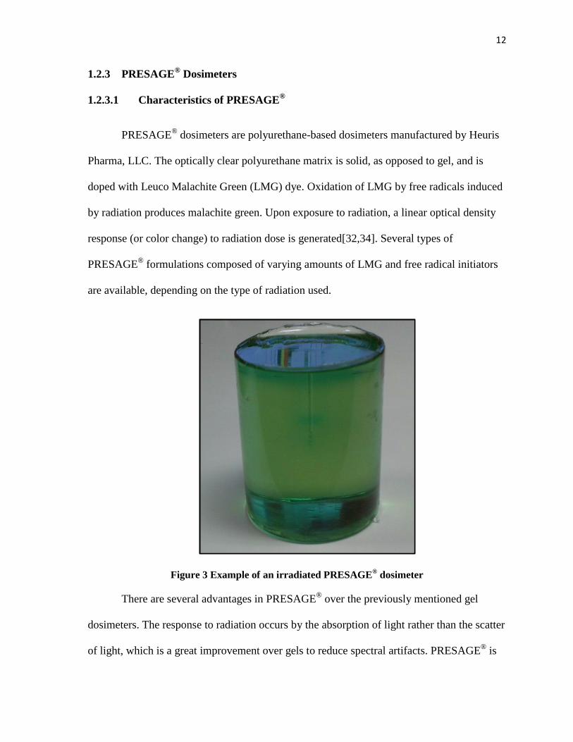
1.2.3 PRESAGE® Dosimeters
1.2.3.1 Characteristics of PRESAGE®
PRESAGE® dosimeters are polyurethane-based dosimeters manufactured by Heuris
Pharma, LLC. The optically clear polyurethane matrix is solid, as opposed to gel, and is
doped with Leuco Malachite Green (LMG) dye. Oxidation of LMG by free radicals induced
by radiation produces malachite green. Upon exposure to radiation, a linear optical density
response (or color change) to radiation dose is generated[32,34]. Several types of
PRESAGE® formulations composed of varying amounts of LMG and free radical initiators
are available, depending on the type of radiation used.
Figure 3 Example of an irradiated PRESAGE® dosimeter
There are several advantages in PRESAGE® over the previously mentioned gel
dosimeters. The response to radiation occurs by the absorption of light rather than the scatter
of light, which is a great improvement over gels to reduce spectral artifacts. PRESAGE® is
13
not sensitive to atmospheric gases, which removes any potential oxygen-induced
inaccuracies and makes it much more convenient to use. An external container for support is
also not necessary, which greatly reduces edge artifacts from optical-CT imaging[35]. This
also allows for PRESAGE® to be easily synthesized into any desirable shape and size.
From 2006 to 2008, Guo et al, J. Adamovics et al, and Sakhalkar et al paved the way
for PRESAGE® by thoroughly evaluating and characterizing the dosimeter response to
radiation. The PRESAGE® dose response does not demonstrate any dependence on external
beam photon energy nor dose rate. Irradiations with the photon energies of 1.25 MeV (Co-
60), 6 MV, 10 MV, and 18 MV all displayed linear dose responses[34,35]. Electrons at the
specific energy of 16 MeV were also evaluated and shown to demonstrate a linear response
in PRESAGE®[32]
. Dose rates ranging from 0.66 Gy min-1
to 10 Gy min-1
showed linearity in
OD change up to doses as high as 50 Gy[34].
Unlike Fricke gel, diffusion of the malachite green does not occur in the
polyurethane[34]. The dose response in PRESAGE® is stable within the first few hours post-
irradiation, although certain formulations have shown that the signal can fade over time[35]
or increase in response (color bleaching) by about 4% per 24 hour period post-
irradiation[34,35]. To account for any signal deviation post-irradiation, a calibration curve
for the change in OD to absolute dose is typically generated through irradiating several
PRESAGE® cuvettes (from the same manufactured batch of PRESAGE
® dosimeters) to a
range of known doses. The cuvettes are read-out following the same irradiation to dose read-
out time scale as used for the experimental dosimeters. This not only accounts for any signal
changes post-irradiation, but also quantifies the sensitivity of PRESAGE® for each batch
14
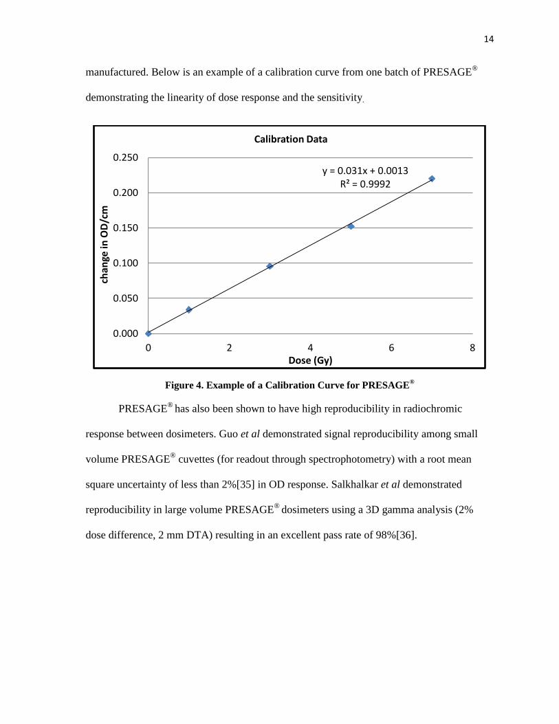
manufactured. Below is an example of a calibration curve from one batch of PRESAGE®
demonstrating the linearity of dose response and the sensitivity.
Figure 4. Example of a Calibration Curve for PRESAGE®
PRESAGE®
has also been shown to have high reproducibility in radiochromic
response between dosimeters. Guo et al demonstrated signal reproducibility among small
volume PRESAGE® cuvettes (for readout through spectrophotometry) with a root mean
square uncertainty of less than 2%[35] in OD response. Salkhalkar et al demonstrated
reproducibility in large volume PRESAGE®
dosimeters using a 3D gamma analysis (2%
dose difference, 2 mm DTA) resulting in an excellent pass rate of 98%[36].
y = 0.031x + 0.0013 R² = 0.9992
0.000
0.050
0.100
0.150
0.200
0.250
0 2 4 6 8
ch
ange
in O
D/c
m
Dose (Gy)
Calibration Data
15
1.2.3.2 Optical-CT Imaging
1.2.3.2.1 The OCTOPUS®
The first scanning system coupled with the introduction of the PRESAGE®
dosimetry system was the OCTOPUS, an optical tomographic system designed by Gore et
al. in 1995. The scanner is available commercially (MGS Research Inc., Madison, CT) and
provides a more time-efficient and cost-effective method of imaging both polymer gels and
PRESAGE® dosimeters over the use of MRI for dosimeter readout. The basic setup of the
scanner includes several mirrors that direct the 633 nm He-Ne laser beam (approximately 1
mm in diameter) to a reference photodiode for the initial light intensity, projections through
the imaging tank, and finally to the photodiode array where the resulting light intensities are
captured. The OCTOPUS was designed to produce linear scans so that one projection
represents the intensities of one horizontal line across the dosimeter. Once all the line
projections are acquired for one slice, the dosimeter is mechanically shifted vertically to a
different level for acquisition of the next slice. Line projection acquisitions for each slice is
repeated until the dosimeter has made a full 360º rotation[32]. The final 3D OD distribution
is then reconstructed using filtered backprojection in MATLAB (The Math Works, Natick,
MA).
The basic principles of using optical-CT to readout dose response in gel or
PRESAGE® dosimeters can be understood with the basic equation[28]:
The laser beam is attenuated exponentially by µ(x,y), the optical attenuation coefficient per
path length (y) at position (x) in the dosimeter. Io is the intensity of the incident
16
monochromatic laser beam and I(x) is the final intensity of the laser beam captured by the
photodiode detector array. By measuring the initial and final intensities of the laser beam,
the OD (or absorbance) can be calculated with the following equation:
While the OCTOPUS is a convenient, commercially-available scanner for 3D
dosimeters, the line-by-line raster scanning is still time consuming. For example, it takes
approximately 7 minutes to scan 150 line projections over one slice[32]. Assuming a slice is
acquired every 2 degrees, it takes approximately 21 hours to scan one dosimeter. In 2010,
Andrew Thomas and Mark Oldham introduced a faster and improved optical-CT design[37].
1.2.3.2.2 Duke Mid-Sized Optical-CT Scanner (DMOS)
The DMOS at the Radiological Physics Center was modeled after the Duke Large
Field-of-view Optical-CT Scanner (DLOS), manufactured by Thomas et al. from Duke
University Medical Center. The scanner was specifically designed for scanning PRESAGE®
dosimeters. Instead of scanning one line at a time, this broad beam scanner is designed to
capture all line-integrals at one projection angle simultaneously. Each projection angle can
be acquired within seconds, thus reducing the scan time from several hours to just 10-20
minutes.
The DLOS/PRESAGE® system has been commissioned to be a 3D dosimetry
system, demonstrating the highest spatial resolution at 0.5 mm size voxels with an MTF of
15%, good contrast up to 1 lp/mm, a dynamic range of at least 60 dB (corresponding to an
17
optical density up to 3 cm-1
), and low image noise after flood and dark corrected projection
images[38].
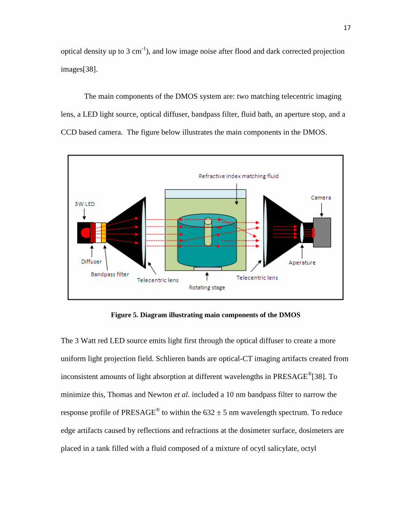
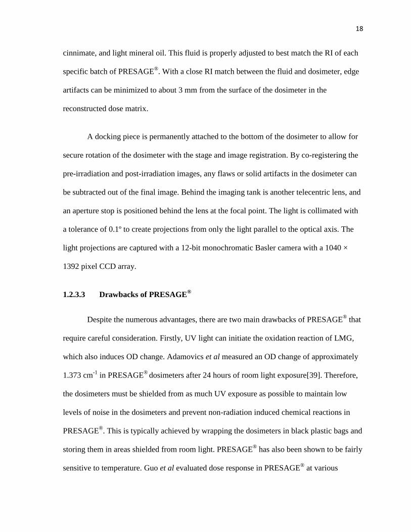
The main components of the DMOS system are: two matching telecentric imaging
lens, a LED light source, optical diffuser, bandpass filter, fluid bath, an aperture stop, and a
CCD based camera. The figure below illustrates the main components in the DMOS.
Figure 5. Diagram illustrating main components of the DMOS
The 3 Watt red LED source emits light first through the optical diffuser to create a more
uniform light projection field. Schlieren bands are optical-CT imaging artifacts created from
inconsistent amounts of light absorption at different wavelengths in PRESAGE®[38]. To
minimize this, Thomas and Newton et al. included a 10 nm bandpass filter to narrow the
response profile of PRESAGE® to within the 632 ± 5 nm wavelength spectrum. To reduce
edge artifacts caused by reflections and refractions at the dosimeter surface, dosimeters are
placed in a tank filled with a fluid composed of a mixture of ocytl salicylate, octyl
18
cinnimate, and light mineral oil. This fluid is properly adjusted to best match the RI of each
specific batch of PRESAGE®. With a close RI match between the fluid and dosimeter, edge
artifacts can be minimized to about 3 mm from the surface of the dosimeter in the
reconstructed dose matrix.
A docking piece is permanently attached to the bottom of the dosimeter to allow for
secure rotation of the dosimeter with the stage and image registration. By co-registering the
pre-irradiation and post-irradiation images, any flaws or solid artifacts in the dosimeter can
be subtracted out of the final image. Behind the imaging tank is another telecentric lens, and
an aperture stop is positioned behind the lens at the focal point. The light is collimated with
a tolerance of 0.1º to create projections from only the light parallel to the optical axis. The
light projections are captured with a 12-bit monochromatic Basler camera with a 1040 ×
1392 pixel CCD array.
1.2.3.3 Drawbacks of PRESAGE®
Despite the numerous advantages, there are two main drawbacks of PRESAGE® that
require careful consideration. Firstly, UV light can initiate the oxidation reaction of LMG,
which also induces OD change. Adamovics et al measured an OD change of approximately
1.373 cm-1
in PRESAGE®
dosimeters after 24 hours of room light exposure[39]. Therefore,
the dosimeters must be shielded from as much UV exposure as possible to maintain low
levels of noise in the dosimeters and prevent non-radiation induced chemical reactions in
PRESAGE®. This is typically achieved by wrapping the dosimeters in black plastic bags and
storing them in areas shielded from room light. PRESAGE® has also been shown to be fairly
sensitive to temperature. Guo et al evaluated dose response in PRESAGE® at various
19
temperatures and concluded that the change in OD versus irradiation temperature is non-
linear. PRESAGE® response increases with temperature due to higher radiochromic activity
at elevated temperatures. To minimize background noise and non-linear radiochromic
effects, the dosimeters are stored at 4°C until time of use. The dosimeters are also
maintained at a constant temperature as best as possible throughout the pre-irradiation
optical-CT scanning, irradiations, and post-irradiation optical-CT scanning processes. For
absolute dose measurements, it is crucial to scan and irradiate PRESAGE® cuvettes at the
same constant temperature the dosimeters were maintained at during the experimental
process to preserve the OD changes as accurately as possible.
1.2.3.4 Previous work with PRESAGE®
Several studies have verified the feasibility and accuracy of PRESAGE® in capturing
the 3D dosimetry of simple to complex IMRT treatment plans. In 2006, Guo et al
demonstrated the feasibility of capturing 3D dose distributions in PRESAGE®
by irradiating
EBT film and PRESAGE® dosimeters with basic 5-beam open-field treatments with 6 MV
photons. Their initial findings through 2D and 3D gamma analysis with the film and the
ECLIPSE® treatment planning system (TPS) resulted in high passing rates for doses above
20% of 15 Gy prescribed to isocenter with a gamma criteria of 4% dose difference and 4
mm distance-to-agreement (DTA)[32]. In 2008, Oldham et al published comprehensive
experimental data which verified the high precision and accuracy of PRESAGE® for
complex IMRT plans. The authors created an 11 field coplanar plan with six small planning
tumor volumes (PTVs) and a large organ-at-risk (OAR) region surrounding the PTVs. The
resulting pass rates of 96% for the 3D gamma analysis with the ECLIPSE®
TPS (3%, 3 mm
DTA) and 91.4% for the 3D gamma analysis with EBT film (3%, 3 mm DTA) proved
20
PRESAGE®
to be a better dosimeter for IMRT treatments[4]. Sakhalkar and Sterling et al
published comparable gamma analysis results in cylindrical PRESAGE® inserts for the
Radiological Physics Center (RPC) Head and Neck (H&N) IMRT phantom used for clinical
trial credentialing purposes[40]. In 2010, Clift et al demonstrated good reproducibility (up to
4%) of radiosurgery field commissioning data in PRESAGE® with respect to film and mini-
ion chambers[41].
3D dosimetry studies in PRESAGE® for proton therapy and brachytherapy have been
ongoing as well, although conclusive quantitative results for dosimeter characterizations
have yet to be published. Heard et al and Al-Nowais et al have investigated the dependence
on LET in PRESAGE® for proton beams[42,43] and future characterization of the dosimeter
for proton therapy is expected. In 2009, Wai et al compared anisotropy functions for
distances at r = 1 cm and r = 2 cm of an HDR 192
Ir source measured in PRESAGE® to
MCNP Monte Carlo calculations and EBT film[44]. The results showed agreement within
3% at 1 cm for anisotropy functions measured in PRESAGE® compared to their Monte
Carlo study for a Nucletron microSelectron-HDR source. More extensive work for the
characterization of PRESAGE® dosimeters for brachytherapy is necessary, especially for
LDR sources. With established accuracy of PRESAGE® in measuring brachytherapy
sources, new brachytherapy sources can be characterized through 3D dosimetry in
PRESAGE®.
21
1.3 Hypothesis and Specific Aims
The hypothesis of this study is that PRESAGE®
dosimeters can reliably measure the
3D dosimetry of brachytherapy sources within ±5% to characterize the dosimetric
parameters of the new AgX100 125
I seed following the protocol specified by TG43-U1.
The specific aims for testing this hypothesis:
1. Develop a suitable PRESAGE® design for single brachytherapy source dosimetry,
determine a suitable set-up for irradiation, and create a method for dose analysis.
2. Compare the measured and published consensus dosimetric parameters in AAPM
TG-43U1 for the Amersham 6711 125
I seed to establish PRESAGE® as a
brachytherapy dosimeter.
3. Measure the delivered dose distribution and dosimetric parameters in PRESAGE®
following the TG-43 formalism for the AgX100 125
I source model.
2 Materials and Methods
2.1 Dosimeter Design
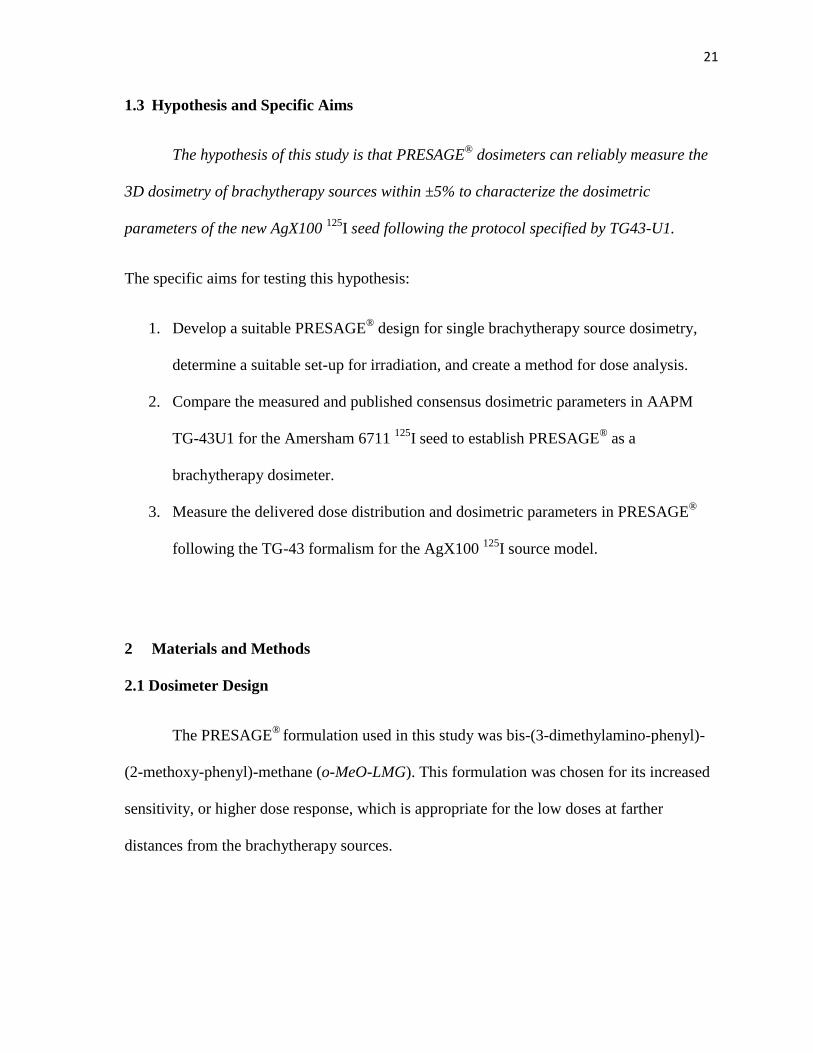
The PRESAGE®
formulation used in this study was bis-(3-dimethylamino-phenyl)-
(2-methoxy-phenyl)-methane (o-MeO-LMG). This formulation was chosen for its increased
sensitivity, or higher dose response, which is appropriate for the low doses at farther
distances from the brachytherapy sources.
22
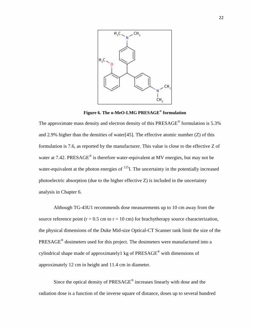
Figure 6. The o-MeO-LMG PRESAGE® formulation
The approximate mass density and electron density of this PRESAGE® formulation is 5.3%
and 2.9% higher than the densities of water[45]. The effective atomic number (Z) of this
formulation is 7.6, as reported by the manufacturer. This value is close to the effective Z of
water at 7.42. PRESAGE® is therefore water-equivalent at MV energies, but may not be
water-equivalent at the photon energies of 125
I. The uncertainty in the potentially increased
photoelectric absorption (due to the higher effective Z) is included in the uncertainty
analysis in Chapter 6.
Although TG-43U1 recommends dose measurements up to 10 cm away from the
source reference point (r = 0.5 cm to r = 10 cm) for brachytherapy source characterization,
the physical dimensions of the Duke Mid-size Optical-CT Scanner tank limit the size of the
PRESAGE® dosimeters used for this project. The dosimeters were manufactured into a
cylindrical shape made of approximately1 kg of PRESAGE® with dimensions of
approximately 12 cm in height and 11.4 cm in diameter.
Since the optical density of PRESAGE® increases linearly with dose and the
radiation dose is a function of the inverse square of distance, doses up to several hundred
23
gray in the immediate vicinity of the source will result in a very large dose response (ie. the
dye in the PRESAGE® matrix becomes very dark in color), which may affect the amount of
light transmittance through the dosimeter in the optical-CT scanner. The minimum relative
dose value that still produces an approximate dose response in PRESAGE® was estimated in
this study to be at approximately 20 cGy based on preliminary experiments. The maximum
dose that produces an accurate dose response has been estimated to be around 50 Gy based
on previous studies[34]. Since the dosimeters are approximately 11.4 cm in diameter, dose
measurements at r = 5 cm is the farthest distance away from the source that can be measured
in the dosimeters used in this project. For the dose to be 20 cGy at 5 cm, the dose at 1 cm
must be approximately 10.5 Gy or 181 Gy at 0.25 cm.
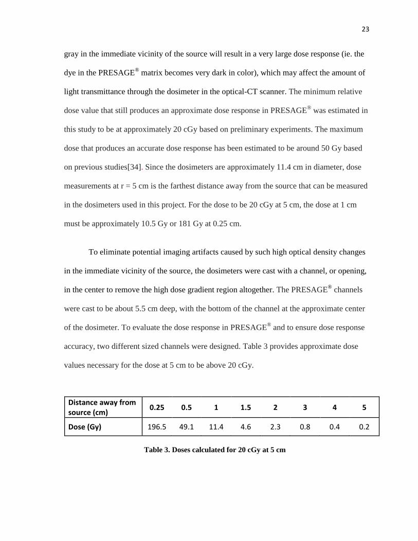
To eliminate potential imaging artifacts caused by such high optical density changes
in the immediate vicinity of the source, the dosimeters were cast with a channel, or opening,
in the center to remove the high dose gradient region altogether. The PRESAGE® channels
were cast to be about 5.5 cm deep, with the bottom of the channel at the approximate center
of the dosimeter. To evaluate the dose response in PRESAGE® and to ensure dose response
accuracy, two different sized channels were designed. Table 3 provides approximate dose
values necessary for the dose at 5 cm to be above 20 cGy.
Distance away from source (cm)
0.25 0.5 1 1.5 2 3 4 5
Dose (Gy) 196.5 49.1 11.4 4.6 2.3 0.8 0.4 0.2
Table 3. Doses calculated for 20 cGy at 5 cm
24
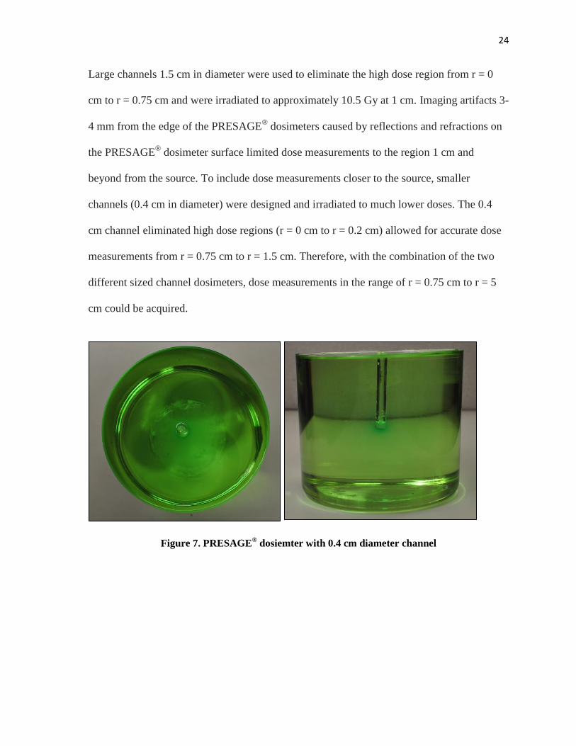
Large channels 1.5 cm in diameter were used to eliminate the high dose region from r = 0
cm to r = 0.75 cm and were irradiated to approximately 10.5 Gy at 1 cm. Imaging artifacts 3-
4 mm from the edge of the PRESAGE® dosimeters caused by reflections and refractions on
the PRESAGE® dosimeter surface limited dose measurements to the region 1 cm and
beyond from the source. To include dose measurements closer to the source, smaller
channels (0.4 cm in diameter) were designed and irradiated to much lower doses. The 0.4
cm channel eliminated high dose regions (r = 0 cm to r = 0.2 cm) allowed for accurate dose
measurements from r = 0.75 cm to r = 1.5 cm. Therefore, with the combination of the two
different sized channel dosimeters, dose measurements in the range of r = 0.75 cm to r = 5
cm could be acquired.
Figure 7. PRESAGE® dosiemter with 0.4 cm diameter channel
25
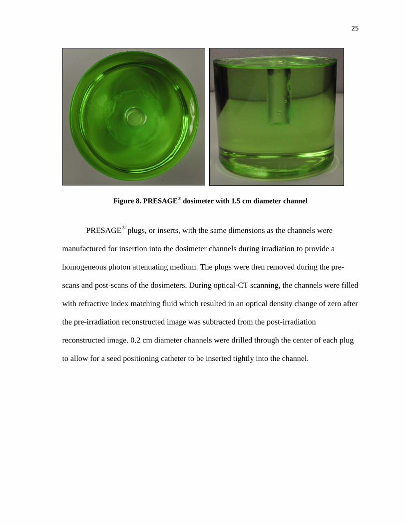
Figure 8. PRESAGE® dosimeter with 1.5 cm diameter channel
PRESAGE® plugs, or inserts, with the same dimensions as the channels were
manufactured for insertion into the dosimeter channels during irradiation to provide a
homogeneous photon attenuating medium. The plugs were then removed during the pre-
scans and post-scans of the dosimeters. During optical-CT scanning, the channels were filled
with refractive index matching fluid which resulted in an optical density change of zero after
the pre-irradiation reconstructed image was subtracted from the post-irradiation
reconstructed image. 0.2 cm diameter channels were drilled through the center of each plug
to allow for a seed positioning catheter to be inserted tightly into the channel.
26
Figure 9 PRESAGE® plugs for 0.4 cm diameter channel
Figure 10 PRESAGE® plugs for 1.5 cm diameter channels
For both 125
I irradiations, a single seed was positioned at the bottom of a 1 mm diameter
thin, plastic catheter. The main purposes of the catheter were to allow for secure insertion of
the radioactive seed, easy removal of the seed from the bottom of the channel, and to ensure
consistent positioning of the seed for each irradiation.
27
Figure 11. Catheter inserted into the 0.4 cm diameter PRESAGE® plug with bottom portion
extended out for visualization purposes
2.2 Treatment Set-up and Delivery
2.2.1 Pre-Irradiation
Upon receiving the dosimeters shipped from Heuris Pharma, LLC, the PRESAGE®
dosimeters were stored at 4° C and concealed from direct light exposure to reduce
background radiochromic response[34]. Prior to pre-irradiation optical-CT scanning, the
dosimeters were removed from the refrigerator and stored at room temperature for a
minimum of four hours to allow for the dosimeters to thaw back to room temperature.
Maintaining the dosimeters at a constant temperature from the start of the pre-irradiation
scans to the end of the post-irradiation scans is believed to be crucial for consistency in dose
28
response. Dosimeters were scanned using the DMOS twenty-four hours prior to irradiation
to capture background signal.
2.2.2 Dose Calibration
Several 1 × 1 × 4.3 cm3 plastic cuvettes filled with PRESAGE
® from the same batch
as the dosimeters were used for dose calibration.
Figure 12. PRESAGE® cuvettes for dose calibration
Although radiochromic response in PRESAGE® has been shown to be independent of dose
rate and photon energy at clinically relevant doses[34], the low photon energy range emitted
by 125
I sources has not been thoroughly evaluated in previous studies. To maintain accurate
calibration, the PRESAGE® cuvettes were irradiated with an orthovoltage unit at 75 kVp
(mean energy around 25 keV) to mimic the weighted mean photon energy of 28 keV emitted
by the 125
I radioactive decay.
29
Prior to irradiation, the absorbance of each cuvette was determined at 633 nm using a
Genesys 20 spectrophotometer (Thermo Scientific, Waltham, MA) to measure the
background optical density. Four cuvettes were irradiated to 1, 3, 5, and 7 Gy. A fifth
cuvette was left un-irradiated to measure change in optical density over the time duration.
The setup for the cuvette irradiation is shown in Figure 13.
Figure 13. PRESAGE® cuvette setup at orthovoltage unit for calibration
Solid water slabs were stacked to create a total thickness of 10 cm to account for backscatter
radiation. Since the depth of maximum dose at 75 kVp is at the surface (SSD=50 cm), the
cuvettes were placed on the top of the solid water setup in the center of an acrylic piece
manufactured by the MDACC machine shop. Any air gaps between the cuvette and acrylic
30
were filled with old PRESAGE® cuvettes and water for consistent material electron
densities.
After irradiation, the absorbance of each cuvette at 633 nm was measured again with
a spectrophotometer. The change in optical density per cm (OD/cm) was determined by
calculating the difference between the pre- and post-irradiation spectrophotometer readings.
The calibration curve was used to convert the OD (per cm) values to the approximate
radiation dose in Gray.
2.2.3 Treatment Delivery
To include backscatter radiation in PRESAGE® dosimetry, an appropriate water-
equivalent material was investigated. Ideally, a dosimeter positioned in the center of a large
water-filled tank for the duration of the irradiation would be the simplest and more accurate
method of capturing the backscatter radiation. However, since PRESAGE®
is partially
soluble in water, white rice grains were selected as the backscatter material instead for its
easier manageability and effectiveness.
Dosimeters were first wrapped in a black plastic zip-lock bag to shield the
PRESAGE® from room light and to also serve as an outer protective cover for the dosimeter
to prevent potential scratches on the surface of the dosimeter from the dry rice grains. The
dosimeter was then placed in the center of plastic tank, and the tank was filled to the top
with the rice grains. The rice grains created approximately 5 cm of backscatter material
around the dosimeter.
31
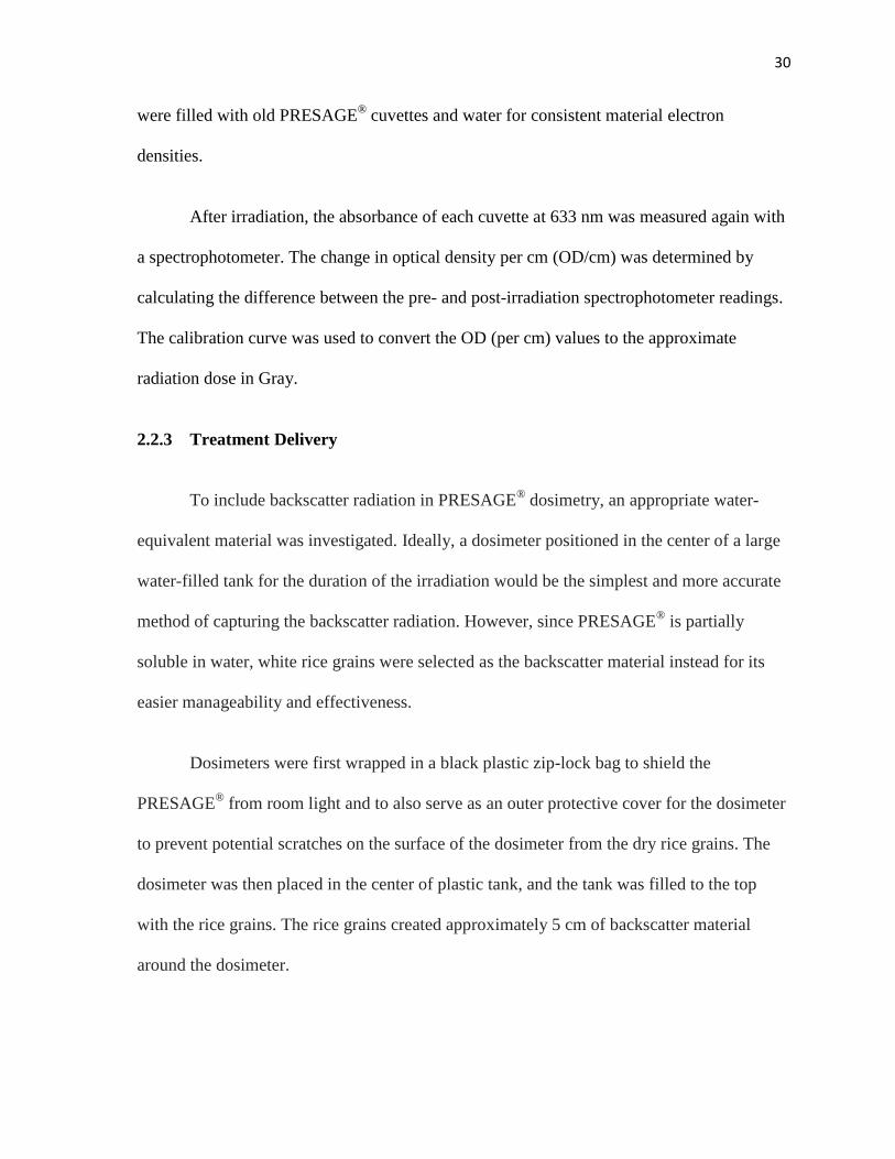
Figure 14. Dosimeter (shielded from light) positioned in rice tank for backscatter
An Amersham 6711 seed with an activity of approximately 9 U was inserted into the
catheter, and the catheter was positioned in the PRESAGE® plug such that the end of the
catheter and the bottom of the seed were both as close to the bottom edge of the plug as
possible. The plug was then fully inserted into the PRESAGE® channel for the duration of
the irradiation. Figure 15 illustrates this configuration.
32
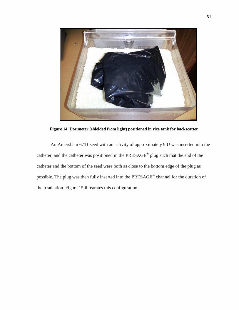
Figure 15. Dosimeter with plug, catheter, and 6711 seed
Dosimeters with 0.4 cm diameter channels were irradiated to 2.5 Gy at 1 cm for dose values
in the range r = 0.75 to 1.5 cm. Dosimeters with 1.5 cm diameter channels were irradiated to
10.5 Gy at 1 cm for dose measurements in the range r = 1.5 to 5.0 cm. The irradiation times
were approximately 25 hours and 138 hours for the small and large channel dosimeters
respectively. The dosimeters were imaged within 4 hours post-irradiation.
An AgX100 source of approximately 6 U in air kerma strength provided by
Theragenics Corporation (Buford, GA) was used for the small channel and large channel
irradiation experiments using the same set-up as the experiments for the Amersham 6711.
Since the seed has only been commercially-available for less than two years, seed strengths
above 2 U are still in the experimental phase (not yet available for purchase). In an attempt
to produce a higher activity seed, the manufacturer, for this project, used a 7 μm plating
33
thickness compared to the routine plating thickness of about 2 μm for the seed. The
irradiation set-up was identical to the Amersham 6711 set-up. Radiation doses were
increased to 3.6 Gy and 12.5 Gy at 1 cm for the small and large channel dosimeters in an
attempt to improve dose response at larger radial distances. The time durations for the small
and large channel dosimeter irradiations were approximately 45 hours (1.9 days) and 237
hours (9.9 days).
2.3 Imaging and Analysis
2.3.1 Optical-CT Imaging
To capture the change in optical density, each dosimeter was scanned prior to and
post-irradiation to capture the background and final OD in the dosimeter. The dosimeters
were imaged with a total of 720 projection images, with projection images taken every 0.5°
rotation. Flood images were taken prior to imaging the dosimeter to capture inhomogeneities
in the matching fluid and LED light field. Dark field images were also captured to correct
for electronic noise.
34
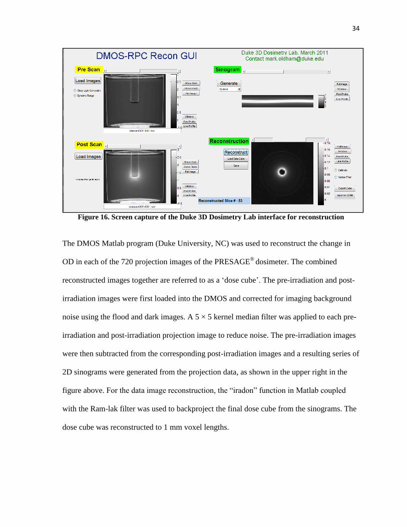
Figure 16. Screen capture of the Duke 3D Dosimetry Lab interface for reconstruction
The DMOS Matlab program (Duke University, NC) was used to reconstruct the change in
OD in each of the 720 projection images of the PRESAGE®
dosimeter. The combined
reconstructed images together are referred to as a ‘dose cube’. The pre-irradiation and post-
irradiation images were first loaded into the DMOS and corrected for imaging background
noise using the flood and dark images. A 5 × 5 kernel median filter was applied to each pre-
irradiation and post-irradiation projection image to reduce noise. The pre-irradiation images
were then subtracted from the corresponding post-irradiation images and a resulting series of
2D sinograms were generated from the projection data, as shown in the upper right in the
figure above. For the data image reconstruction, the “iradon” function in Matlab coupled
with the Ram-lak filter was used to backproject the final dose cube from the sinograms. The
dose cube was reconstructed to 1 mm voxel lengths.
35
2.3.2 Data Acquisition in CERR
The reconstructed dose cube showing the resulting radiation-induced optical density
changes were imported from the DMOS program into the Computational Environment for
Radiotherapy Research (CERR) platform. CERR is a widely-used and free Matlab software
used to display and analyze treatment plans in radiation therapy research[46]. Once loaded
into CERR, the change in OD values were scaled to dose values using the scale factor
obtained from the calibration curve.
PRESAGE® is suspected to have volume effects that may affect the accuracy of dose
values when the conversion factor for pixel to dose values, obtained from small volume
PRESAGE®, is applied to large 1 kg PRESAGE
® dosimeters. Therefore, the converted dose
values in CERR are re-normalized to the dose at r =1.5 cm on the transverse bisecting plane
of the seed. The relative dose values in PRESAGE® are measured in CERR using the “Dose
Line Profile” tool. This tool function captures each dose pixel value along the user-selected
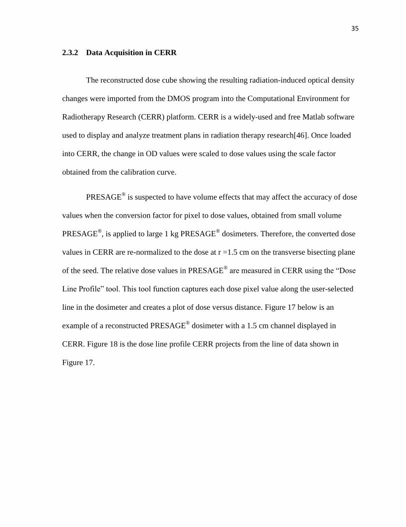
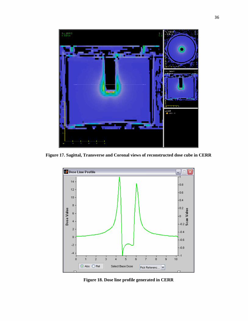
line in the dosimeter and creates a plot of dose versus distance. Figure 17 below is an
example of a reconstructed PRESAGE® dosimeter with a 1.5 cm channel displayed in
CERR. Figure 18 is the dose line profile CERR projects from the line of data shown in
Figure 17.
36
Figure 17. Sagittal, Transverse and Coronal views of reconstructed dose cube in CERR
Figure 18. Dose line profile generated in CERR
37
For the purposes of this study, dose values with the corresponding distances from the dose-
line profile were then exported into an Excel workbook for further dose and analysis.
2.4 TG-43 Formalism
The recommended formalism established in the AAPM TG-43 report and followed
by the TG-43U1 report is defined here for purposes of clarification and easier understanding
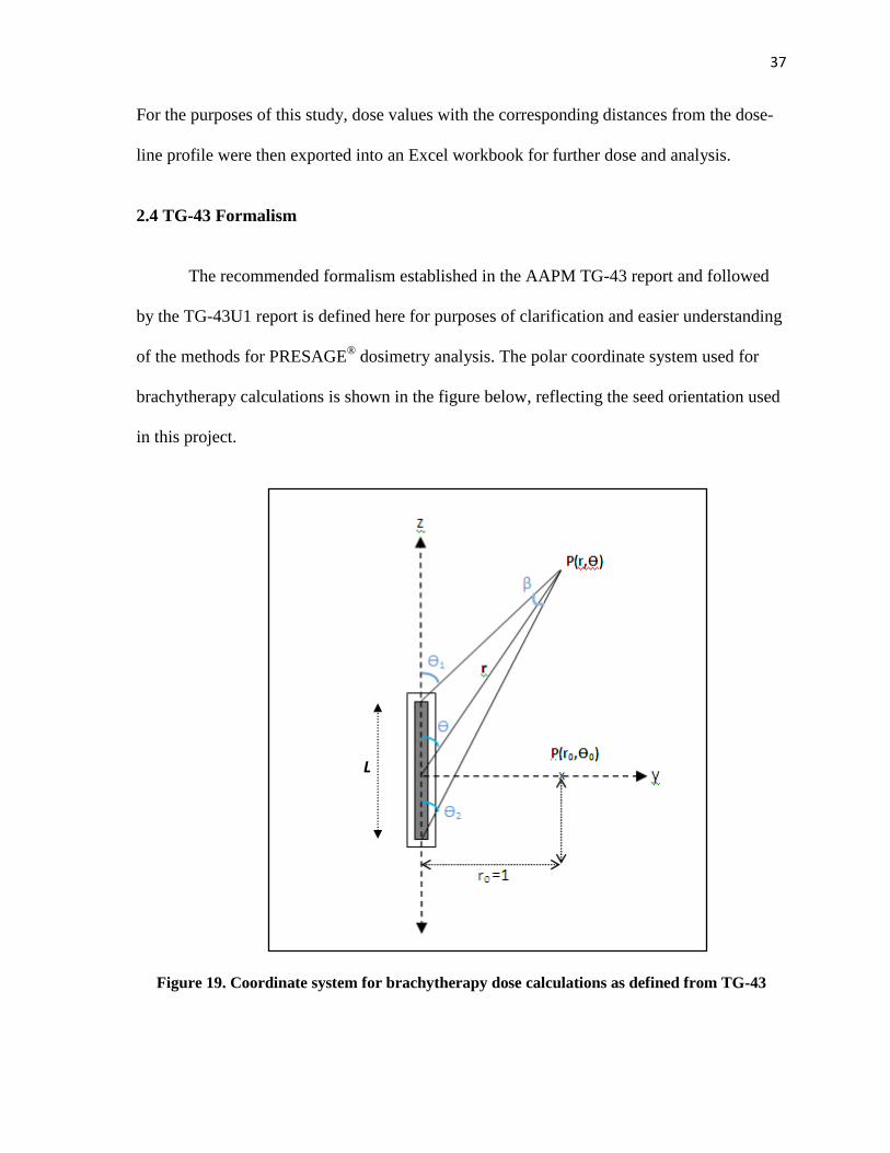
of the methods for PRESAGE® dosimetry analysis. The polar coordinate system used for
brachytherapy calculations is shown in the figure below, reflecting the seed orientation used
in this project.
Figure 19. Coordinate system for brachytherapy dose calculations as defined from TG-43
L
38
L is the active length of the seed in centimeters. r is defined as the distance in centimeters
from the center of the source to the point of interest and Ѳ is the polar angle created between
r and the longitudinal bisecting plane of the seed. Therefore, denotes the
coordinates for the point of interest. TG-43 defines the reference point at the
distance of r = 1 cm and Ѳ = 90° or π/2 radians, as shown in the Figure 17. The accuracy of
the reference point in measurements is crucial because the anisotropy and radial dose
function values are dependent on the dose rate at this point.
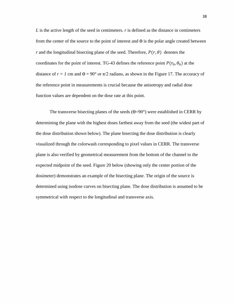
The transverse bisecting planes of the seeds (Ѳ=90°) were established in CERR by
determining the plane with the highest doses farthest away from the seed (the widest part of
the dose distribution shown below). The plane bisecting the dose distribution is clearly
visualized through the colorwash corresponding to pixel values in CERR. The transverse
plane is also verified by geometrical measurement from the bottom of the channel to the
expected midpoint of the seed. Figure 20 below (showing only the center portion of the
dosimeter) demonstrates an example of the bisecting plane. The origin of the source is
determined using isodose curves on bisecting plane. The dose distribution is assumed to be
symmetrical with respect to the longitudinal and transverse axis.
39
Figure 20. Transverse bisecting plane determined in CERR
2.4.1 Air-kerma Strength
As re-defined in the TG-43U1 report, the radioactive strength of brachytherapy
sources is described by , the air-kerma strength in units of ), and
is defined by the following equation:
is the air-kerma rate corrected for in-air photon attenuation and scattering (for air-
kerma “in vacuo”) at distance d from the center of the transverse bisecting plane of the
source to the point at which the air-kerma was measured. δ is the lower bound energy cutoff
for air-kerma rate measurement and is typically set at δ = 5 keV. Photons below this energy
are usually created through interactions with the titanium seed capsule and do not contribute
to patient dose beyond r = 0.1 cm. The air-kerma strength values are typically reported by

40
the manufacturer or calibrated by an Accredited Dosimetry Calibration Laboratory (ADCL)
and are traceable to the 1999 National Standards Institute of Technology (NIST) standard.
The air-kerma strengths of the brachytherapy seeds used in this study were calibrated
by the ADCL at the MD Anderson Cancer Center. Since ADCLs have direct traceability to
the NIST primary standards, using the air-kerma strength provided by the ADCL reduces the
uncertainty in dose measurements.
2.4.2 Dose rate
The 2D dose-rate (cGy h-1
) to water equation is specified in the TG-43 protocol:
This 2D dose rate equation was used to calculate dose rates to water for comparison with the
measured dose rates in PRESAGE®. The consensus dose rates (cGy h
-1 U
-1) as a function of
radial distance (r) for each of the source models are shown in the tables below.
r (cm) 1.0 1.5 2.0 3.0 4.0 5.0
Dose rate
(cGy h-1 U-1) 0.9650 0.3910 0.1975 0.0681 0.0301 0.0141
Table 4. Dose rate using 2D formalism for the Amersham 6711
r (cm) 1.0 1.5 2.0 3.0 4.0 5.0
Dose rate
(cGy h-1 U-1) 0.9530 0.3862 0.1950 0.0673 0.0297 0.0140
Table 5. Dose rates using 2D formalism for the AgX100
41
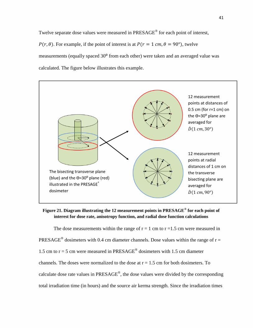
Twelve separate dose values were measured in PRESAGE® for each point of interest,
. For example, if the point of interest is at , twelve
measurements (equally spaced 30⁰ from each other) were taken and an averaged value was
calculated. The figure below illustrates this example.
Figure 21. Diagram illustrating the 12 measurement points in PRESAGE® for each point of
interest for dose rate, anisotropy function, and radial dose function calculations
The dose measurements within the range of r = 1 cm to r =1.5 cm were measured in
PRESAGE® dosimeters with 0.4 cm diameter channels. Dose values within the range of r =
1.5 cm to r = 5 cm were measured in PRESAGE®
dosimeters with 1.5 cm diameter
channels. The doses were normalized to the dose at r = 1.5 cm for both dosimeters. To
calculate dose rate values in PRESAGE®
, the dose values were divided by the corresponding
total irradiation time (in hours) and the source air kerma strength. Since the irradiation times
12 measurement
points at radial
distances of 1 cm on
the transverse
bisecting plane are
averaged for
12 measurement
points at distances of
0.5 cm (for r=1 cm) on
the Ѳ=30⁰ plane are
averaged for
The bisecting transverse plane
(blue) and the Ѳ=30⁰ plane (red)
illustrated in the PRESAGE®
dosimeter
42
for the larger dosimeters were up to almost 10 days, a decay correction was included in the
dose calculations for cumulated dose. The total cumulative dose for a “temporary implant”
in brachytherapy can be calculated using the equation below[47] .
Therefore, the equation to calculate the dose rate (cGy h-1
U-1
) at each radial distance
from the mean dose measurements, , in PRESAGE® is shown in the equation below.
2.4.3 Dose Rate Constant
The dose rate constant in water, Λ, has the units of cGy h-1
U-1
and is defined as the
ratio of the dose rate at the reference point to the air-kerma strength:
The dose rate constant is dependent on the source model design. The consensus dose rate
constant values reported in TG-43U1 (including the value for the Amersham 6711) were
derived by taking the equally-weighted average of the experimentally measured dose rate
constants and the Monte Carlo calculated dose rate constants. Since the AgX100 seed is
new, a consensus dose rate constant recommended by a consensus value recommended by
an AAPM task group is not yet available. However, Theragenics uses the equally-weighted
mean of the dose rate constants measured through Monte Carlo calculations and
43
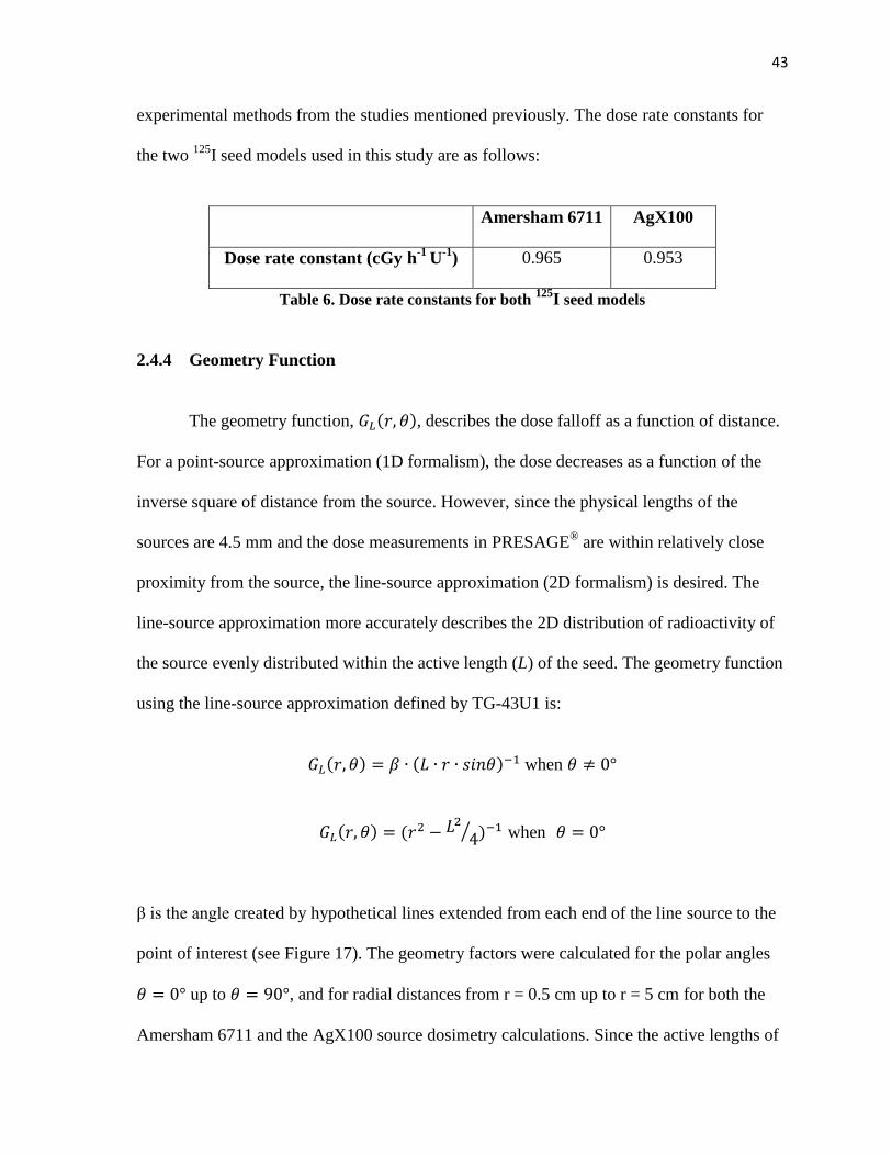
experimental methods from the studies mentioned previously. The dose rate constants for
the two 125
I seed models used in this study are as follows:
Amersham 6711 AgX100
Dose rate constant (cGy h-1
U-1
) 0.965 0.953
Table 6. Dose rate constants for both 125
I seed models
2.4.4 Geometry Function
The geometry function, , describes the dose falloff as a function of distance.
For a point-source approximation (1D formalism), the dose decreases as a function of the
inverse square of distance from the source. However, since the physical lengths of the
sources are 4.5 mm and the dose measurements in PRESAGE® are within relatively close
proximity from the source, the line-source approximation (2D formalism) is desired. The
line-source approximation more accurately describes the 2D distribution of radioactivity of
the source evenly distributed within the active length (L) of the seed. The geometry function
using the line-source approximation defined by TG-43U1 is:
when
when
β is the angle created by hypothetical lines extended from each end of the line source to the
point of interest (see Figure 17). The geometry factors were calculated for the polar angles
up to , and for radial distances from r = 0.5 cm up to r = 5 cm for both the
Amersham 6711 and the AgX100 source dosimetry calculations. Since the active lengths of
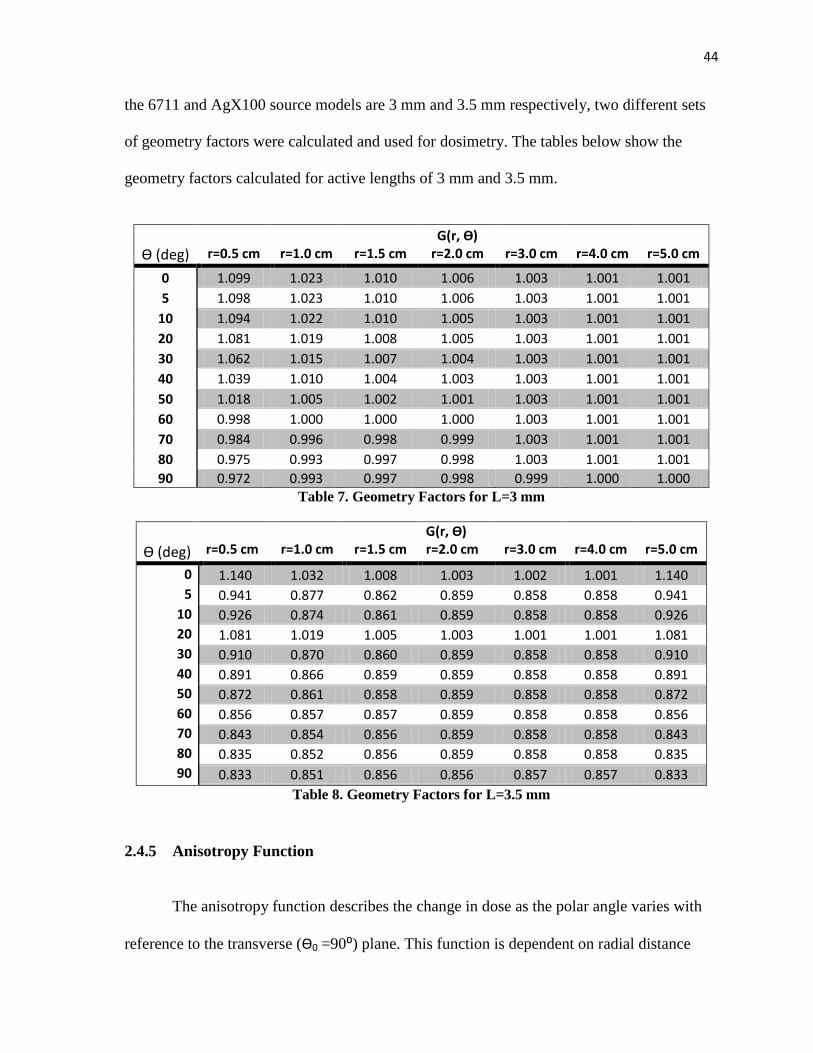
44
the 6711 and AgX100 source models are 3 mm and 3.5 mm respectively, two different sets
of geometry factors were calculated and used for dosimetry. The tables below show the
geometry factors calculated for active lengths of 3 mm and 3.5 mm.
Ѳ (deg)
r=0.5 cm
r=1.0 cm
r=1.5 cm
G(r, Ѳ) r=2.0 cm
r=3.0 cm
r=4.0 cm
r=5.0 cm
0 1.099 1.023 1.010 1.006 1.003 1.001 1.001
5 1.098 1.023 1.010 1.006 1.003 1.001 1.001
10 1.094 1.022 1.010 1.005 1.003 1.001 1.001
20 1.081 1.019 1.008 1.005 1.003 1.001 1.001
30 1.062 1.015 1.007 1.004 1.003 1.001 1.001
40 1.039 1.010 1.004 1.003 1.003 1.001 1.001
50 1.018 1.005 1.002 1.001 1.003 1.001 1.001
60 0.998 1.000 1.000 1.000 1.003 1.001 1.001
70 0.984 0.996 0.998 0.999 1.003 1.001 1.001
80 0.975 0.993 0.997 0.998 1.003 1.001 1.001
90 0.972 0.993 0.997 0.998 0.999 1.000 1.000 Table 7. Geometry Factors for L=3 mm
Ѳ (deg)
r=0.5 cm
r=1.0 cm
r=1.5 cm
G(r, Ѳ) r=2.0 cm
r=3.0 cm
r=4.0 cm
r=5.0 cm
0 1.140 1.032 1.008 1.003 1.002 1.001 1.140 5 0.941 0.877 0.862 0.859 0.858 0.858 0.941
10 0.926 0.874 0.861 0.859 0.858 0.858 0.926 20 1.081 1.019 1.005 1.003 1.001 1.001 1.081 30 0.910 0.870 0.860 0.859 0.858 0.858 0.910 40 0.891 0.866 0.859 0.859 0.858 0.858 0.891 50 0.872 0.861 0.858 0.859 0.858 0.858 0.872 60 0.856 0.857 0.857 0.859 0.858 0.858 0.856 70 0.843 0.854 0.856 0.859 0.858 0.858 0.843 80 0.835 0.852 0.856 0.859 0.858 0.858 0.835 90 0.833 0.851 0.856 0.856 0.857 0.857 0.833
Table 8. Geometry Factors for L=3.5 mm
2.4.5 Anisotropy Function
The anisotropy function describes the change in dose as the polar angle varies with
reference to the transverse (Ѳ0 =90⁰) plane. This function is dependent on radial distance
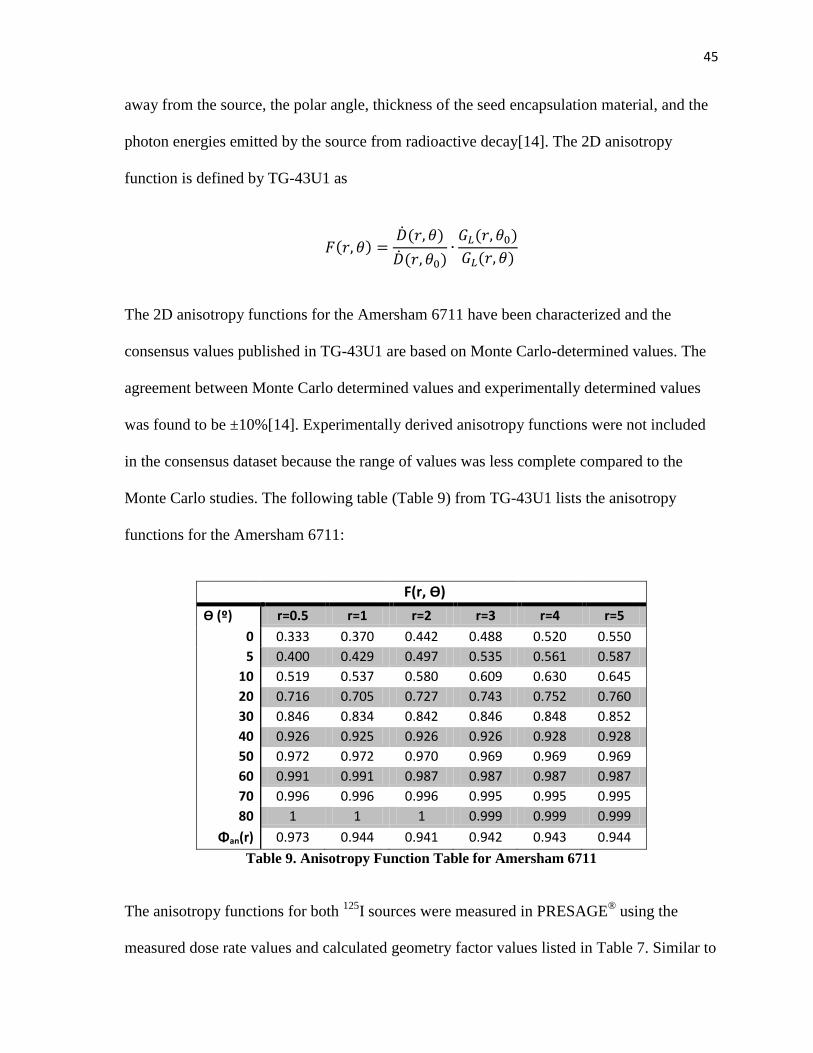
45
away from the source, the polar angle, thickness of the seed encapsulation material, and the
photon energies emitted by the source from radioactive decay[14]. The 2D anisotropy
function is defined by TG-43U1 as
The 2D anisotropy functions for the Amersham 6711 have been characterized and the
consensus values published in TG-43U1 are based on Monte Carlo-determined values. The
agreement between Monte Carlo determined values and experimentally determined values
was found to be ±10%[14]. Experimentally derived anisotropy functions were not included
in the consensus dataset because the range of values was less complete compared to the
Monte Carlo studies. The following table (Table 9) from TG-43U1 lists the anisotropy
functions for the Amersham 6711:
F(r, Ѳ)
Ѳ (º) r=0.5 r=1 r=2 r=3 r=4 r=5
0 0.333 0.370 0.442 0.488 0.520 0.550
5 0.400 0.429 0.497 0.535 0.561 0.587
10 0.519 0.537 0.580 0.609 0.630 0.645
20 0.716 0.705 0.727 0.743 0.752 0.760
30 0.846 0.834 0.842 0.846 0.848 0.852
40 0.926 0.925 0.926 0.926 0.928 0.928
50 0.972 0.972 0.970 0.969 0.969 0.969
60 0.991 0.991 0.987 0.987 0.987 0.987
70 0.996 0.996 0.996 0.995 0.995 0.995
80 1 1 1 0.999 0.999 0.999
Φan(r) 0.973 0.944 0.941 0.942 0.943 0.944
Table 9. Anisotropy Function Table for Amersham 6711
The anisotropy functions for both 125
I sources were measured in PRESAGE® using the
measured dose rate values and calculated geometry factor values listed in Table 7. Similar to
46
the measurements for the dose rates in PRESAGE®, twelve separate point dose values were
measured in PRESAGE®
for each anisotropy function and the mean of the dose values was
converted to dose rate and used to calculate the mean anisotropy function for each point of
interest. For example, to calculate , twelve points (30º apart) on the
plane were measured and averaged. The dose rate (cGy h-1
U-1
) was
determined from the mean dose value by dividing by the total irradiation time in hours and
the air kerma strength (corrected for the radioactive decay). The mean dose rate,
, was then divided by the mean dose rate on the transverse plane
, and multiplied by the ratio of geometry factors to obtain the anisotropy
function measured in PRESAGE®. The measured anisotropy
functions for the Amersham 6711 were compared to the Monte Carlo anisotropy functions to
evaluate the accuracy of brachytherapy dose measurements in PRESAGE® dosimeters.
2.4.6 Radial Dose Function
The radial dose function describes the change in radiation dose due to scattering and
attenuation of photons on the transverse plane, excluding the dose fall-off due to the inverse
square law (already accounted for by the geometry function)[14]. The 2D equation for the
radial dose function using the line-source approximation is:
Monte Carlo derived values and experimentally measured values of the radial dose function
show an average agreement of ±10%[14]. The consensus values recommended by TG-43U1
include datasets mostly from Monte Carlo calculations for radial dose values, especially at
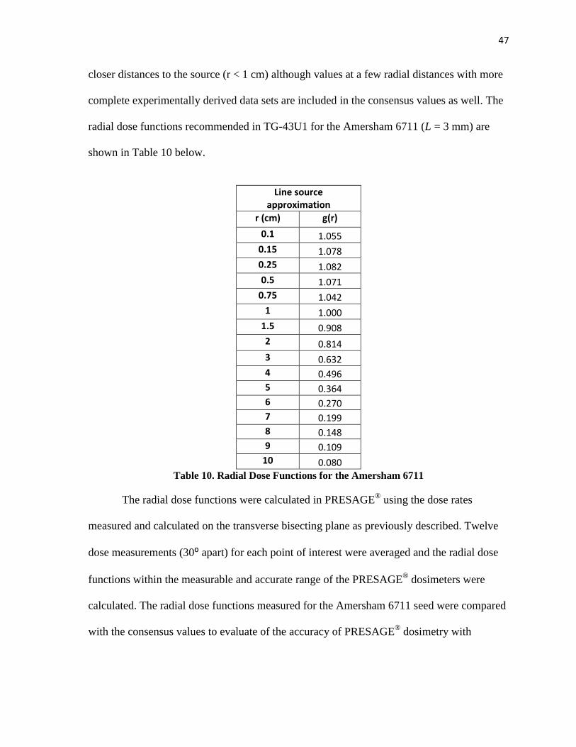
47
closer distances to the source (r < 1 cm) although values at a few radial distances with more
complete experimentally derived data sets are included in the consensus values as well. The
radial dose functions recommended in TG-43U1 for the Amersham 6711 (L = 3 mm) are
shown in Table 10 below.
Line source approximation
r (cm) g(r)
0.1 1.055
0.15 1.078
0.25 1.082
0.5 1.071
0.75 1.042
1 1.000
1.5 0.908
2 0.814
3 0.632
4 0.496
5 0.364
6 0.270
7 0.199
8 0.148
9 0.109
10 0.080
Table 10. Radial Dose Functions for the Amersham 6711
The radial dose functions were calculated in PRESAGE® using the dose rates
measured and calculated on the transverse bisecting plane as previously described. Twelve
dose measurements (30⁰ apart) for each point of interest were averaged and the radial dose
functions within the measurable and accurate range of the PRESAGE® dosimeters were
calculated. The radial dose functions measured for the Amersham 6711 seed were compared
with the consensus values to evaluate of the accuracy of PRESAGE® dosimetry with
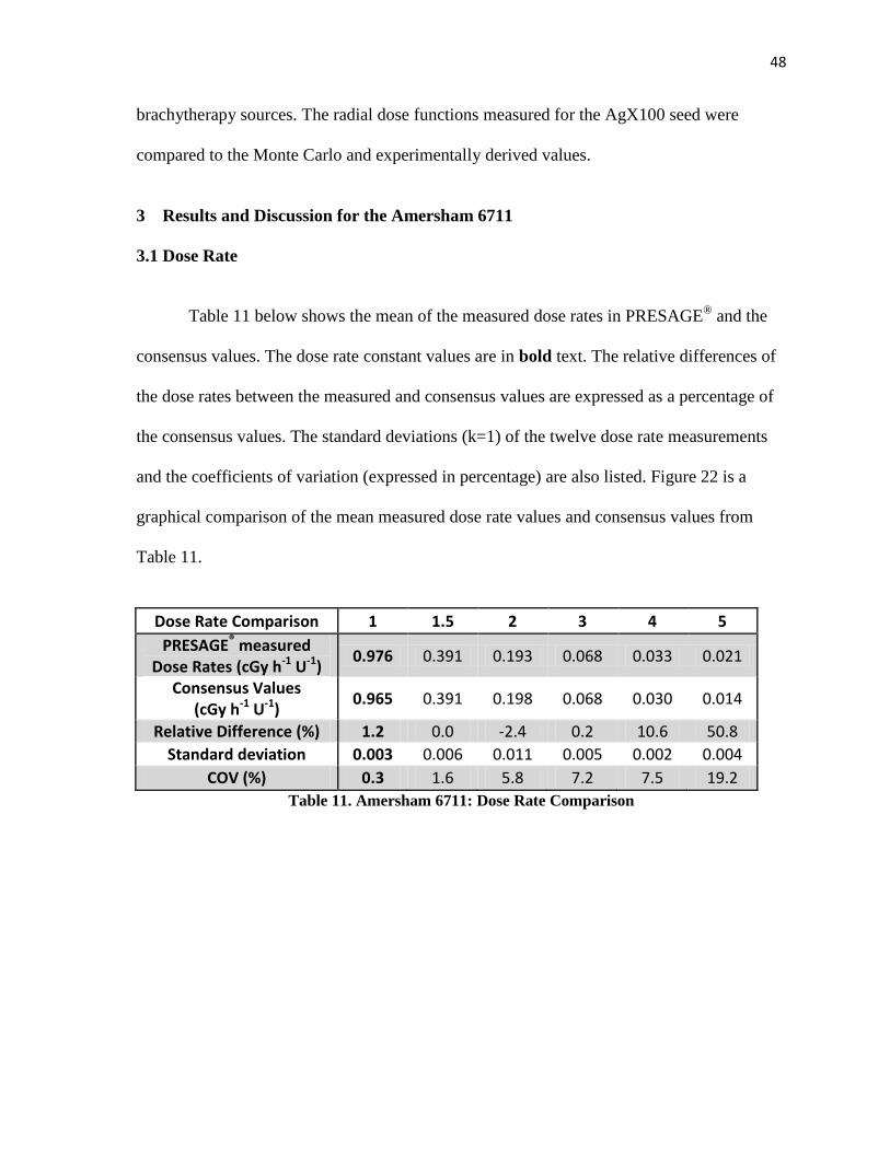
48
brachytherapy sources. The radial dose functions measured for the AgX100 seed were
compared to the Monte Carlo and experimentally derived values.
3 Results and Discussion for the Amersham 6711
3.1 Dose Rate
Table 11 below shows the mean of the measured dose rates in PRESAGE®
and the
consensus values. The dose rate constant values are in bold text. The relative differences of
the dose rates between the measured and consensus values are expressed as a percentage of
the consensus values. The standard deviations (k=1) of the twelve dose rate measurements
and the coefficients of variation (expressed in percentage) are also listed. Figure 22 is a
graphical comparison of the mean measured dose rate values and consensus values from
Table 11.
Dose Rate Comparison 1 1.5 2 3 4 5
PRESAGE® measured Dose Rates (cGy h-1 U-1)
0.976 0.391 0.193 0.068 0.033 0.021
Consensus Values (cGy h-1 U-1)
0.965 0.391 0.198 0.068 0.030 0.014
Relative Difference (%) 1.2 0.0 -2.4 0.2 10.6 50.8
Standard deviation 0.003 0.006 0.011 0.005 0.002 0.004
COV (%) 0.3 1.6 5.8 7.2 7.5 19.2
Table 11. Amersham 6711: Dose Rate Comparison
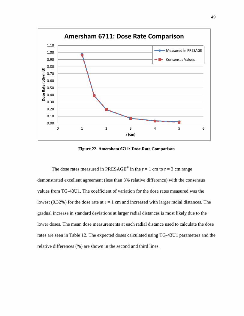
49
Figure 22. Amersham 6711: Dose Rate Comparison
The dose rates measured in PRESAGE® in the r = 1 cm to r = 3 cm range
demonstrated excellent agreement (less than 3% relative difference) with the consensus
values from TG-43U1. The coefficient of variation for the dose rates measured was the
lowest (0.32%) for the dose rate at r = 1 cm and increased with larger radial distances. The
gradual increase in standard deviations at larger radial distances is most likely due to the
lower doses. The mean dose measurements at each radial distance used to calculate the dose
rates are seen in Table 12. The expected doses calculated using TG-43U1 parameters and the
relative differences (%) are shown in the second and third lines.
0.00
0.10
0.20
0.30
0.40
0.50
0.60
0.70
0.80
0.90
1.00
1.10
0 1 2 3 4 5 6
Do
se R
ate
(cG
y/h
U)
r (cm)
Amersham 6711: Dose Rate Comparison
Measured in PRESAGE
Consensus Values
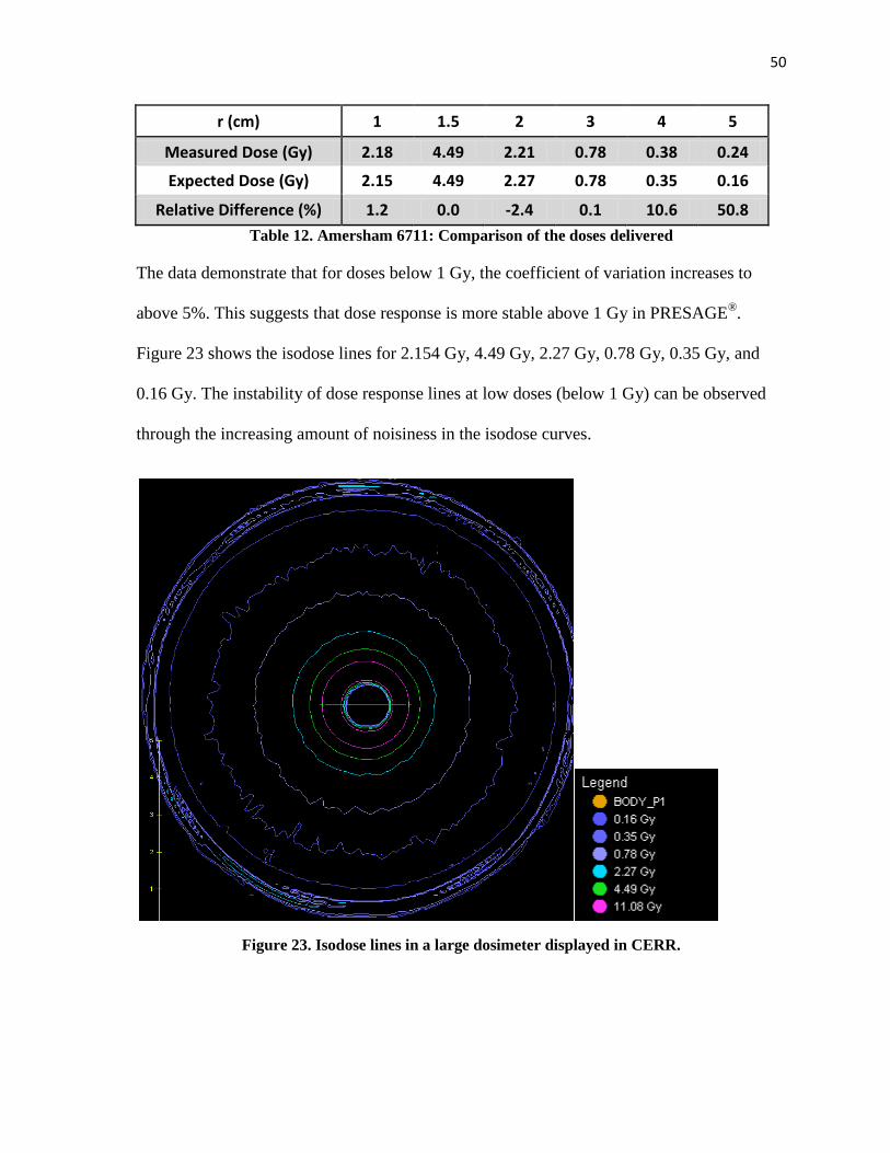
50
r (cm) 1 1.5 2 3 4 5
Measured Dose (Gy) 2.18 4.49 2.21 0.78 0.38 0.24
Expected Dose (Gy) 2.15 4.49 2.27 0.78 0.35 0.16
Relative Difference (%) 1.2 0.0 -2.4 0.1 10.6 50.8
Table 12. Amersham 6711: Comparison of the doses delivered
The data demonstrate that for doses below 1 Gy, the coefficient of variation increases to
above 5%. This suggests that dose response is more stable above 1 Gy in PRESAGE®.
Figure 23 shows the isodose lines for 2.154 Gy, 4.49 Gy, 2.27 Gy, 0.78 Gy, 0.35 Gy, and
0.16 Gy. The instability of dose response lines at low doses (below 1 Gy) can be observed
through the increasing amount of noisiness in the isodose curves.
Figure 23. Isodose lines in a large dosimeter displayed in CERR.
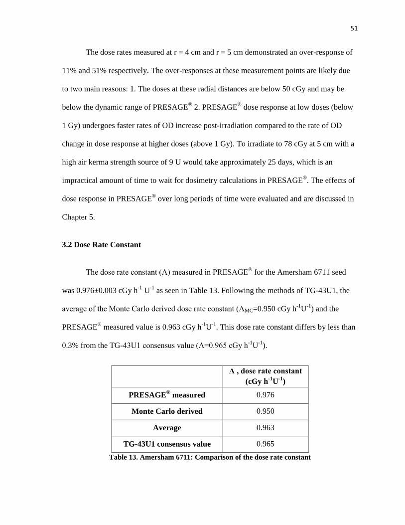
51
The dose rates measured at r = 4 cm and r = 5 cm demonstrated an over-response of
11% and 51% respectively. The over-responses at these measurement points are likely due
to two main reasons: 1. The doses at these radial distances are below 50 cGy and may be
below the dynamic range of PRESAGE®
2. PRESAGE® dose response at low doses (below
1 Gy) undergoes faster rates of OD increase post-irradiation compared to the rate of OD
change in dose response at higher doses (above 1 Gy). To irradiate to 78 cGy at 5 cm with a
high air kerma strength source of 9 U would take approximately 25 days, which is an
impractical amount of time to wait for dosimetry calculations in PRESAGE®. The effects of
dose response in PRESAGE® over long periods of time were evaluated and are discussed in
Chapter 5.
3.2 Dose Rate Constant
The dose rate constant (Λ) measured in PRESAGE® for the Amersham 6711 seed
was 0.976±0.003 cGy h-1
U-1
as seen in Table 13. Following the methods of TG-43U1, the
average of the Monte Carlo derived dose rate constant (ΛMC=0.950 cGy h-1
U-1
) and the
PRESAGE® measured value is 0.963 cGy h
-1U
-1. This dose rate constant differs by less than
0.3% from the TG-43U1 consensus value (Λ=0.965 cGy h-1
U-1
).
Λ , dose rate constant
(cGy h-1
U-1
)
PRESAGE® measured 0.976
Monte Carlo derived 0.950
Average 0.963
TG-43U1 consensus value 0.965
Table 13. Amersham 6711: Comparison of the dose rate constant
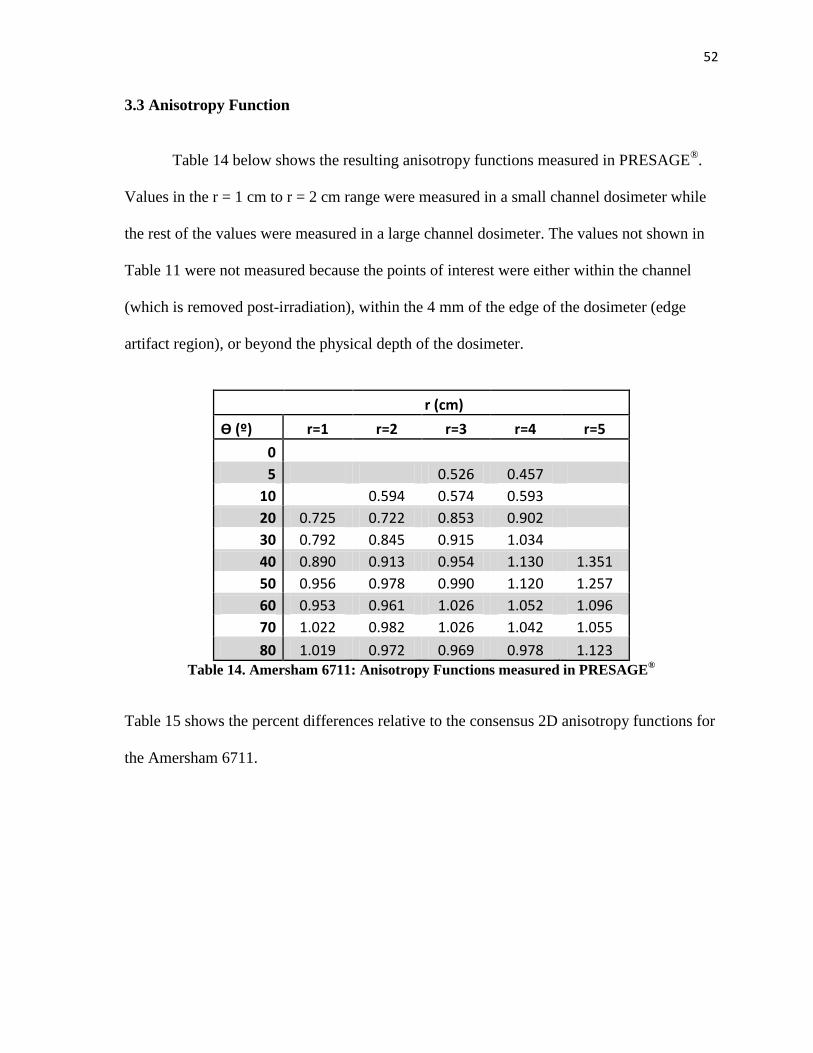
52
3.3 Anisotropy Function
Table 14 below shows the resulting anisotropy functions measured in PRESAGE®
.
Values in the r = 1 cm to r = 2 cm range were measured in a small channel dosimeter while
the rest of the values were measured in a large channel dosimeter. The values not shown in
Table 11 were not measured because the points of interest were either within the channel
(which is removed post-irradiation), within the 4 mm of the edge of the dosimeter (edge
artifact region), or beyond the physical depth of the dosimeter.
r (cm)
Ѳ (º) r=1 r=2 r=3 r=4 r=5
0
5 0.526 0.457
10
0.594 0.574 0.593
20 0.725 0.722 0.853 0.902
30 0.792 0.845 0.915 1.034
40 0.890 0.913 0.954 1.130 1.351
50 0.956 0.978 0.990 1.120 1.257
60 0.953 0.961 1.026 1.052 1.096
70 1.022 0.982 1.026 1.042 1.055
80 1.019 0.972 0.969 0.978 1.123 Table 14. Amersham 6711: Anisotropy Functions measured in PRESAGE
®
Table 15 shows the percent differences relative to the consensus 2D anisotropy functions for
the Amersham 6711.
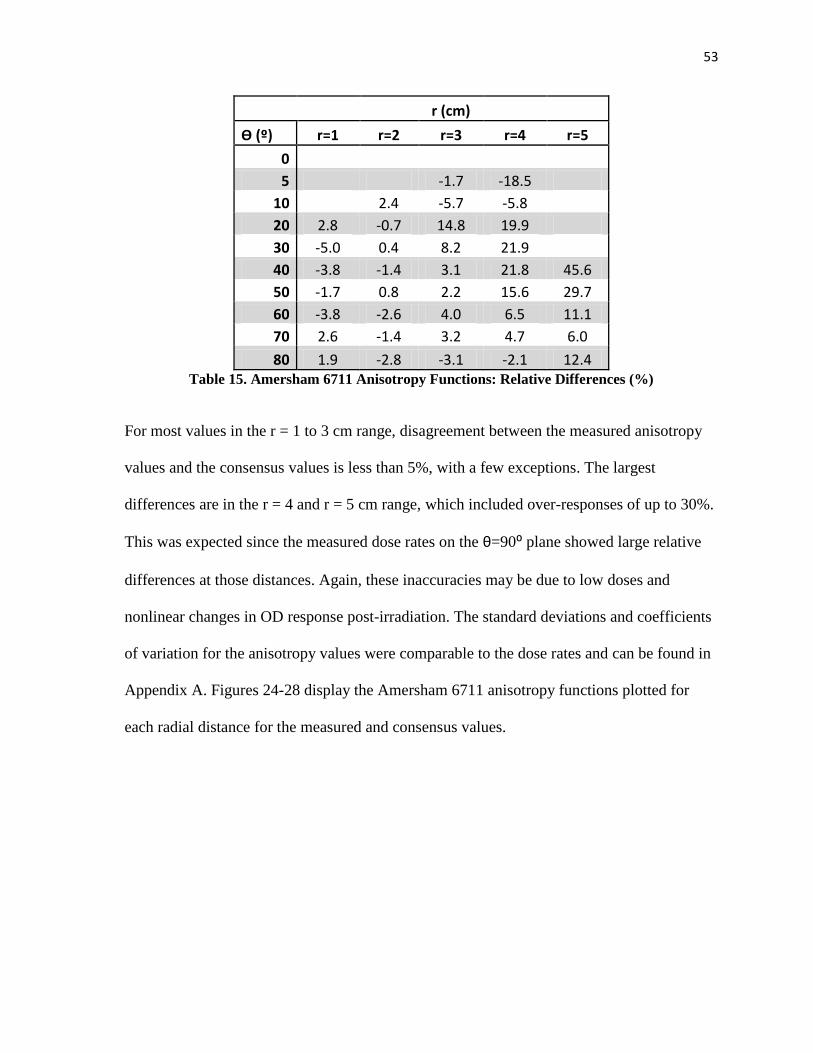
53
r (cm)
Ѳ (º) r=1 r=2 r=3 r=4 r=5
0
5 -1.7 -18.5
10
2.4 -5.7 -5.8
20 2.8 -0.7 14.8 19.9
30 -5.0 0.4 8.2 21.9
40 -3.8 -1.4 3.1 21.8 45.6
50 -1.7 0.8 2.2 15.6 29.7
60 -3.8 -2.6 4.0 6.5 11.1
70 2.6 -1.4 3.2 4.7 6.0
80 1.9 -2.8 -3.1 -2.1 12.4 Table 15. Amersham 6711 Anisotropy Functions: Relative Differences (%)
For most values in the r = 1 to 3 cm range, disagreement between the measured anisotropy
values and the consensus values is less than 5%, with a few exceptions. The largest
differences are in the r = 4 and r = 5 cm range, which included over-responses of up to 30%.
This was expected since the measured dose rates on the θ=90⁰ plane showed large relative
differences at those distances. Again, these inaccuracies may be due to low doses and
nonlinear changes in OD response post-irradiation. The standard deviations and coefficients
of variation for the anisotropy values were comparable to the dose rates and can be found in
Appendix A. Figures 24-28 display the Amersham 6711 anisotropy functions plotted for
each radial distance for the measured and consensus values.
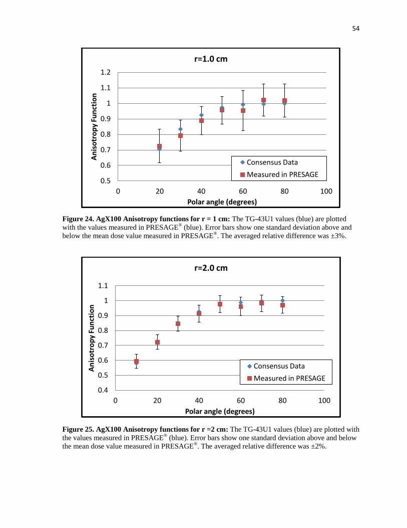
54
Figure 24. AgX100 Anisotropy functions for r = 1 cm: The TG-43U1 values (blue) are plotted
with the values measured in PRESAGE® (blue). Error bars show one standard deviation above and
below the mean dose value measured in PRESAGE®. The averaged relative difference was ±3%.
Figure 25. AgX100 Anisotropy functions for r =2 cm: The TG-43U1 values (blue) are plotted with
the values measured in PRESAGE® (blue). Error bars show one standard deviation above and below
the mean dose value measured in PRESAGE®. The averaged relative difference was ±2%.
0.5
0.6
0.7
0.8
0.9
1
1.1
1.2
0 20 40 60 80 100
An
iso
tro
py
Fun
ctio
n
Polar angle (degrees)
r=1.0 cm
Consensus Data
Measured in PRESAGE
0.4
0.5
0.6
0.7
0.8
0.9
1
1.1
0 20 40 60 80 100
An
iso
tro
py
Fun
ctio
n
Polar angle (degrees)
r=2.0 cm
Consensus Data
Measured in PRESAGE
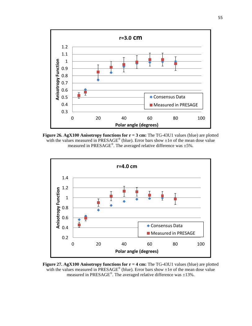
55
Figure 26. AgX100 Anisotropy functions for r = 3 cm: The TG-43U1 values (blue) are plotted
with the values measured in PRESAGE® (blue). Error bars show ±1σ of the mean dose value
measured in PRESAGE®. The averaged relative difference was ±5%.
Figure 27. AgX100 Anisotropy functions for r = 4 cm: The TG-43U1 values (blue) are plotted
with the values measured in PRESAGE® (blue). Error bars show ±1σ of the mean dose value
measured in PRESAGE®. The averaged relative difference was ±13%.
0.3
0.4
0.5
0.6
0.7
0.8
0.9
1
1.1
1.2
0 20 40 60 80 100
An
iso
tro
py
Fun
ctio
n
Polar angle (degrees)
r=3.0 cm
Consensus Data
Measured in PRESAGE
0.2
0.4
0.6
0.8
1
1.2
1.4
0 20 40 60 80 100
An
iso
tro
py
Fun
ctio
n
Polar angle (degrees)
r=4.0 cm
Consensus Data
Measured in PRESAGE
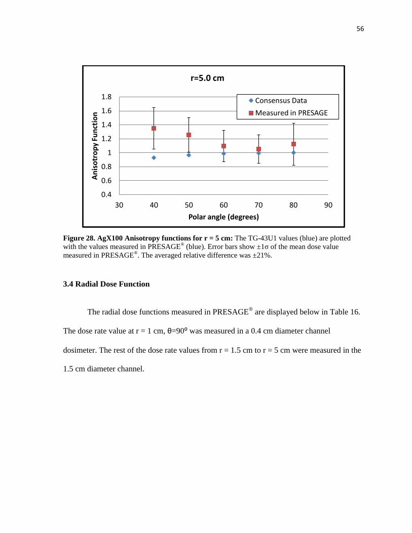
56
Figure 28. AgX100 Anisotropy functions for r = 5 cm: The TG-43U1 values (blue) are plotted
with the values measured in PRESAGE® (blue). Error bars show ±1σ of the mean dose value
measured in PRESAGE®. The averaged relative difference was ±21%.
3.4 Radial Dose Function
The radial dose functions measured in PRESAGE® are displayed below in Table 16.
The dose rate value at r = 1 cm, θ=90⁰ was measured in a 0.4 cm diameter channel
dosimeter. The rest of the dose rate values from r = 1.5 cm to r = 5 cm were measured in the
1.5 cm diameter channel.
0.4
0.6
0.8
1
1.2
1.4
1.6
1.8
30 40 50 60 70 80 90
An
iso
tro
py
Fun
ctio
n
Polar angle (degrees)
r=5.0 cm
Consensus Data
Measured in PRESAGE
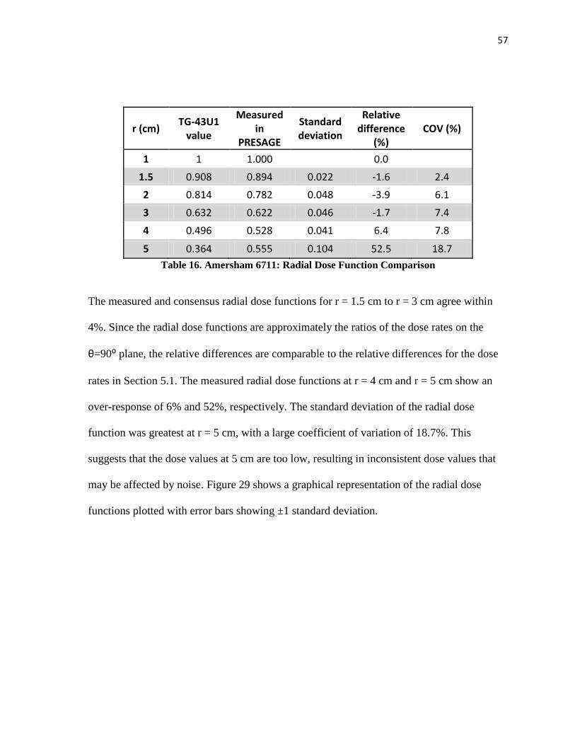
57
r (cm) TG-43U1
value
Measured in
PRESAGE
Standard deviation
Relative difference
(%) COV (%)
1 1 1.000
0.0
1.5 0.908 0.894 0.022 -1.6 2.4
2 0.814 0.782 0.048 -3.9 6.1
3 0.632 0.622 0.046 -1.7 7.4
4 0.496 0.528 0.041 6.4 7.8
5 0.364 0.555 0.104 52.5 18.7
Table 16. Amersham 6711: Radial Dose Function Comparison
The measured and consensus radial dose functions for r = 1.5 cm to r = 3 cm agree within
4%. Since the radial dose functions are approximately the ratios of the dose rates on the
θ=90⁰ plane, the relative differences are comparable to the relative differences for the dose
rates in Section 5.1. The measured radial dose functions at r = 4 cm and r = 5 cm show an
over-response of 6% and 52%, respectively. The standard deviation of the radial dose
function was greatest at r = 5 cm, with a large coefficient of variation of 18.7%. This
suggests that the dose values at 5 cm are too low, resulting in inconsistent dose values that
may be affected by noise. Figure 29 shows a graphical representation of the radial dose
functions plotted with error bars showing ±1 standard deviation.
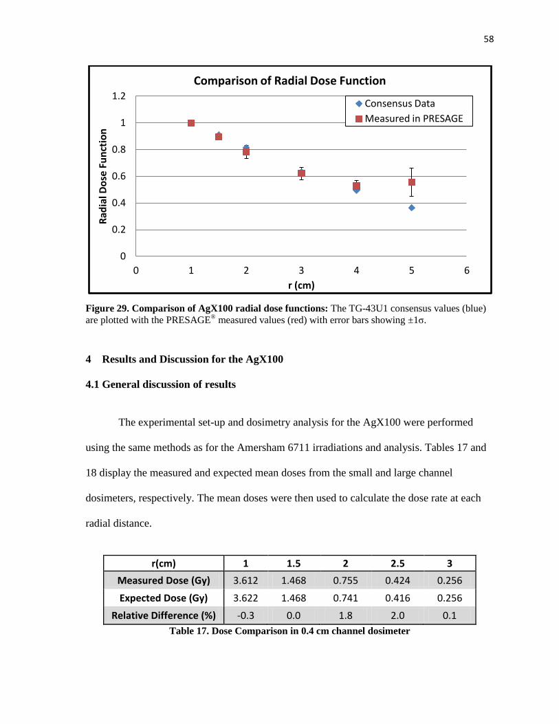
58
Figure 29. Comparison of AgX100 radial dose functions: The TG-43U1 consensus values (blue)
are plotted with the PRESAGE® measured values (red) with error bars showing ±1σ.
4 Results and Discussion for the AgX100
4.1 General discussion of results
The experimental set-up and dosimetry analysis for the AgX100 were performed
using the same methods as for the Amersham 6711 irradiations and analysis. Tables 17 and
18 display the measured and expected mean doses from the small and large channel
dosimeters, respectively. The mean doses were then used to calculate the dose rate at each
radial distance.
r(cm) 1 1.5 2 2.5 3
Measured Dose (Gy) 3.612 1.468 0.755 0.424 0.256
Expected Dose (Gy) 3.622 1.468 0.741 0.416 0.256
Relative Difference (%) -0.3 0.0 1.8 2.0 0.1
Table 17. Dose Comparison in 0.4 cm channel dosimeter
0
0.2
0.4
0.6
0.8
1
1.2
0 1 2 3 4 5 6
Rad
ial D
ose
Fu
nct
ion
r (cm)
Comparison of Radial Dose Function
Consensus Data
Measured in PRESAGE
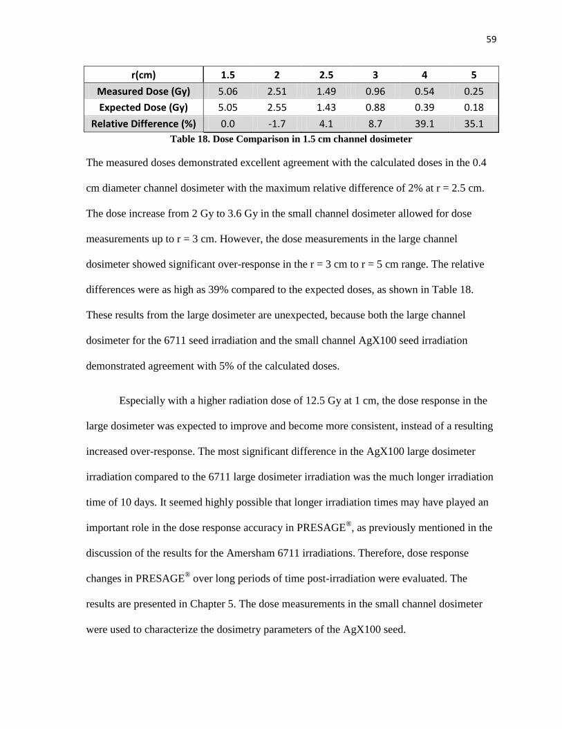
59
r(cm) 1.5 2 2.5 3 4 5
Measured Dose (Gy) 5.06 2.51 1.49 0.96 0.54 0.25
Expected Dose (Gy) 5.05 2.55 1.43 0.88 0.39 0.18
Relative Difference (%) 0.0 -1.7 4.1 8.7 39.1 35.1
Table 18. Dose Comparison in 1.5 cm channel dosimeter
The measured doses demonstrated excellent agreement with the calculated doses in the 0.4
cm diameter channel dosimeter with the maximum relative difference of 2% at r = 2.5 cm.
The dose increase from 2 Gy to 3.6 Gy in the small channel dosimeter allowed for dose
measurements up to r = 3 cm. However, the dose measurements in the large channel
dosimeter showed significant over-response in the r = 3 cm to r = 5 cm range. The relative
differences were as high as 39% compared to the expected doses, as shown in Table 18.
These results from the large dosimeter are unexpected, because both the large channel
dosimeter for the 6711 seed irradiation and the small channel AgX100 seed irradiation
demonstrated agreement with 5% of the calculated doses.
Especially with a higher radiation dose of 12.5 Gy at 1 cm, the dose response in the
large dosimeter was expected to improve and become more consistent, instead of a resulting
increased over-response. The most significant difference in the AgX100 large dosimeter
irradiation compared to the 6711 large dosimeter irradiation was the much longer irradiation
time of 10 days. It seemed highly possible that longer irradiation times may have played an
important role in the dose response accuracy in PRESAGE®, as previously mentioned in the
discussion of the results for the Amersham 6711 irradiations. Therefore, dose response
changes in PRESAGE® over long periods of time post-irradiation were evaluated. The
results are presented in Chapter 5. The dose measurements in the small channel dosimeter
were used to characterize the dosimetry parameters of the AgX100 seed.
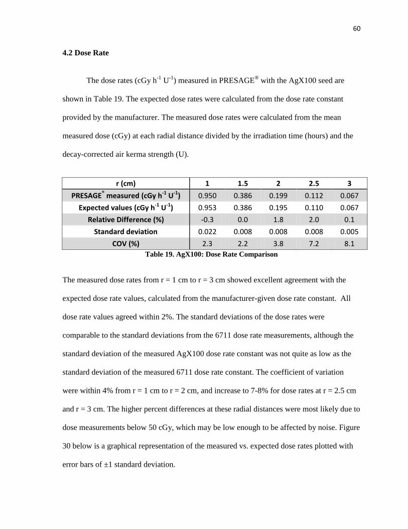
60
4.2 Dose Rate
The dose rates (cGy h-1
U-1
) measured in PRESAGE® with the AgX100 seed are
shown in Table 19. The expected dose rates were calculated from the dose rate constant
provided by the manufacturer. The measured dose rates were calculated from the mean
measured dose (cGy) at each radial distance divided by the irradiation time (hours) and the
decay-corrected air kerma strength (U).
r (cm) 1 1.5 2 2.5 3
PRESAGE® measured (cGy h-1 U-1) 0.950 0.386 0.199 0.112 0.067
Expected values (cGy h-1 U-1) 0.953 0.386 0.195 0.110 0.067
Relative Difference (%) -0.3 0.0 1.8 2.0 0.1
Standard deviation 0.022 0.008 0.008 0.008 0.005
COV (%) 2.3 2.2 3.8 7.2 8.1
Table 19. AgX100: Dose Rate Comparison
The measured dose rates from r = 1 cm to r = 3 cm showed excellent agreement with the
expected dose rate values, calculated from the manufacturer-given dose rate constant. All
dose rate values agreed within 2%. The standard deviations of the dose rates were
comparable to the standard deviations from the 6711 dose rate measurements, although the
standard deviation of the measured AgX100 dose rate constant was not quite as low as the
standard deviation of the measured 6711 dose rate constant. The coefficient of variation
were within 4% from r = 1 cm to r = 2 cm, and increase to 7-8% for dose rates at r = 2.5 cm
and r = 3 cm. The higher percent differences at these radial distances were most likely due to
dose measurements below 50 cGy, which may be low enough to be affected by noise. Figure
30 below is a graphical representation of the measured vs. expected dose rates plotted with
error bars of ±1 standard deviation.
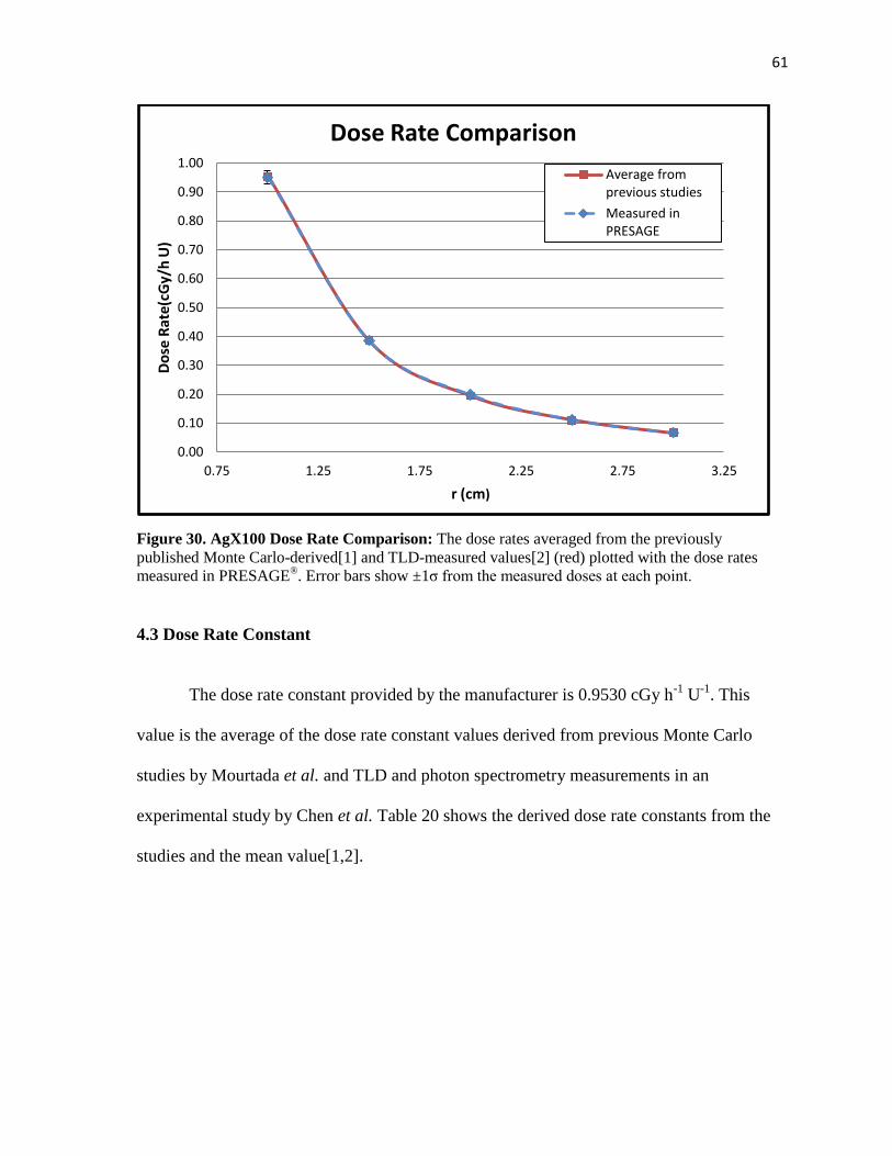
61
Figure 30. AgX100 Dose Rate Comparison: The dose rates averaged from the previously
published Monte Carlo-derived[1] and TLD-measured values[2] (red) plotted with the dose rates
measured in PRESAGE®. Error bars show ±1σ from the measured doses at each point.
4.3 Dose Rate Constant
The dose rate constant provided by the manufacturer is 0.9530 cGy h-1
U-1
. This
value is the average of the dose rate constant values derived from previous Monte Carlo
studies by Mourtada et al. and TLD and photon spectrometry measurements in an
experimental study by Chen et al. Table 20 shows the derived dose rate constants from the
studies and the mean value[1,2].
0.00
0.10
0.20
0.30
0.40
0.50
0.60
0.70
0.80
0.90
1.00
0.75 1.25 1.75 2.25 2.75 3.25
Do
se R
ate(
cGy/
h U
)
r (cm)
Dose Rate Comparison
Average from previous studies
Measured in PRESAGE
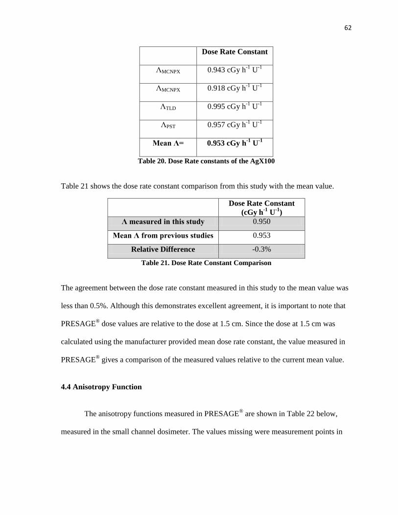
62
Dose Rate Constant
ΛMCNPX 0.943 cGy h-1
U-1
ΛMCNPX 0.918 cGy h-1
U-1
ΛTLD 0.995 cGy h-1
U-1
ΛPST 0.957 cGy h-1
U-1
Mean Λ= 0.953 cGy h-1
U-1
Table 20. Dose Rate constants of the AgX100
Table 21 shows the dose rate constant comparison from this study with the mean value.
Dose Rate Constant
(cGy h-1 U
-1)
Λ measured in this study 0.950
Mean Λ from previous studies 0.953
Relative Difference -0.3%
Table 21. Dose Rate Constant Comparison
The agreement between the dose rate constant measured in this study to the mean value was
less than 0.5%. Although this demonstrates excellent agreement, it is important to note that
PRESAGE® dose values are relative to the dose at 1.5 cm. Since the dose at 1.5 cm was
calculated using the manufacturer provided mean dose rate constant, the value measured in
PRESAGE® gives a comparison of the measured values relative to the current mean value.
4.4 Anisotropy Function
The anisotropy functions measured in PRESAGE® are shown in Table 22 below,
measured in the small channel dosimeter. The values missing were measurement points in
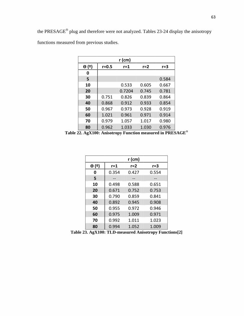
63
the PRESAGE® plug and therefore were not analyzed. Tables 23-24 display the anisotropy
functions measured from previous studies.
r (cm)
Ѳ (º) r=0.5 r=1 r=2 r=3
0 5
0.584
10
0.533 0.605 0.667
20
0.7204 0.745 0.781 30 0.751 0.826 0.839 0.864 40 0.868 0.912 0.933 0.854 50 0.967 0.973 0.928 0.919 60 1.021 0.961 0.971 0.914 70 0.979 1.057 1.017 0.980
80 0.962 1.033 1.030 0.976 Table 22. AgX100: Anisotropy Function measured in PRESAGE
®
r (cm)
Ѳ (º) r=1 r=2 r=3
0 0.354 0.427 0.554 5 -- -- --
10 0.498 0.588 0.651 20 0.671 0.752 0.753 30 0.790 0.859 0.841 40 0.892 0.945 0.908
50 0.955 0.972 0.946
60 0.975 1.009 0.971 70 0.992 1.011 1.023
80 0.994 1.052 1.009 Table 23. AgX100: TLD-measured Anisotropy Functions[2]
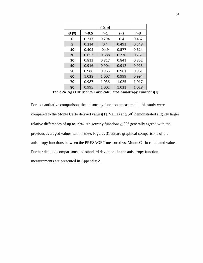
64
r (cm)
Ѳ (º) r=0.5 r=1 r=2 r=3
0 0.217 0.294 0.4 0.462
5 0.314 0.4 0.493 0.548
10 0.404 0.49 0.577 0.624
20 0.652 0.688 0.736 0.761
30 0.813 0.817 0.841 0.852
40 0.916 0.904 0.912 0.915
50 0.986 0.963 0.961 0.961
60 1.028 1.007 0.999 0.994
70 0.987 1.036 1.025 1.017
80 0.995 1.002 1.031 1.028 Table 24. AgX100: Monte-Carlo calculated Anisotropy Functions[1]
For a quantitative comparison, the anisotropy functions measured in this study were
compared to the Monte Carlo derived values[1]. Values at ≤ 30⁰ demonstrated slightly larger
relative differences of up to ±9%. Anisotropy functions ≥ 30⁰ generally agreed with the
previous averaged values within ±5%. Figures 31-33 are graphical comparisons of the
anisotropy functions between the PRESAGE®
-measured vs. Monte Carlo calculated values.
Further detailed comparisons and standard deviations in the anisotropy function
measurements are presented in Appendix A.
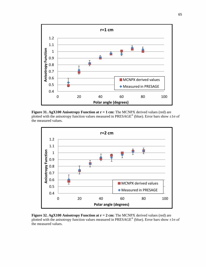
65
Figure 31. AgX100 Anisotropy Function at r = 1 cm: The MCNPX derived values (red) are
plotted with the anisotropy function values measured in PRESAGE® (blue). Error bars show ±1σ of
the measured values.
Figure 32. AgX100 Anisotropy Function at r = 2 cm: The MCNPX derived values (red) are
plotted with the anisotropy function values measured in PRESAGE® (blue). Error bars show ±1σ of
the measured values.
0.4
0.5
0.6
0.7
0.8
0.9
1
1.1
1.2
0 20 40 60 80 100
An
iso
tro
py
Fun
ctio
n
Polar angle (degrees)
r=1 cm
MCNPX derived values
Measured in PRESAGE
0.4
0.5
0.6
0.7
0.8
0.9
1
1.1
1.2
0 20 40 60 80 100
An
iso
tro
py
Fun
ctio
n
Polar angle (degrees)
r=2 cm
MCNPX derived values
Measured in PRESAGE
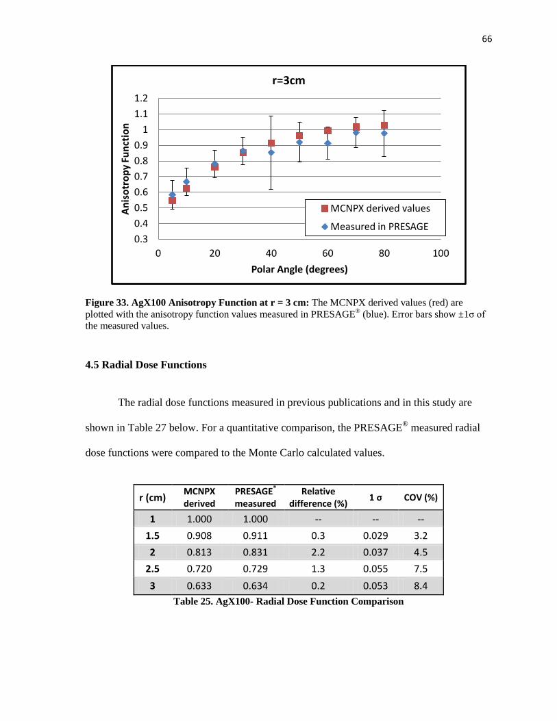
66
Figure 33. AgX100 Anisotropy Function at r = 3 cm: The MCNPX derived values (red) are
plotted with the anisotropy function values measured in PRESAGE® (blue). Error bars show ±1σ of
the measured values.
4.5 Radial Dose Functions
The radial dose functions measured in previous publications and in this study are
shown in Table 27 below. For a quantitative comparison, the PRESAGE® measured radial
dose functions were compared to the Monte Carlo calculated values.
r (cm) MCNPX derived
PRESAGE® measured
Relative difference (%)
1 σ COV (%)
1 1.000 1.000 -- -- --
1.5 0.908 0.911 0.3 0.029 3.2
2 0.813 0.831 2.2 0.037 4.5
2.5 0.720 0.729 1.3 0.055 7.5
3 0.633 0.634 0.2 0.053 8.4
Table 25. AgX100- Radial Dose Function Comparison
0.3
0.4
0.5
0.6
0.7
0.8
0.9
1
1.1
1.2
0 20 40 60 80 100
An
iso
tro
py
Fun
ctio
n
Polar Angle (degrees)
r=3cm
MCNPX derived values
Measured in PRESAGE
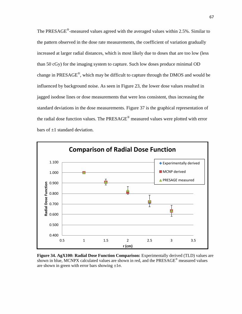
67
The PRESAGE®
-measured values agreed with the averaged values within 2.5%. Similar to
the pattern observed in the dose rate measurements, the coefficient of variation gradually
increased at larger radial distances, which is most likely due to doses that are too low (less
than 50 cGy) for the imaging system to capture. Such low doses produce minimal OD
change in PRESAGE®, which may be difficult to capture through the DMOS and would be
influenced by background noise. As seen in Figure 23, the lower dose values resulted in
jagged isodose lines or dose measurements that were less consistent, thus increasing the
standard deviations in the dose measurements. Figure 37 is the graphical representation of
the radial dose function values. The PRESAGE® measured values were plotted with error
bars of ±1 standard deviation.
Figure 34. AgX100: Radial Dose Function Comparison: Experimentally derived (TLD) values are
shown in blue, MCNPX calculated values are shown in red, and the PRESAGE® measured values
are shown in green with error bars showing ±1σ.
0.400
0.500
0.600
0.700
0.800
0.900
1.000
1.100
0.5 1 1.5 2 2.5 3 3.5
Rad
ial D
ose
Fu
nct
ion
r (cm)
Comparison of Radial Dose Function
Experimentally derived
MCNP derived
PRESAGE measured
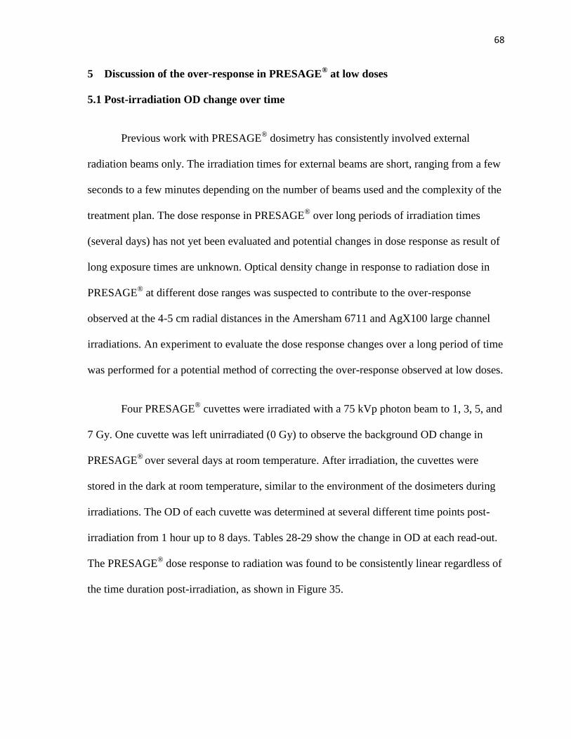
68
5 Discussion of the over-response in PRESAGE® at low doses
5.1 Post-irradiation OD change over time
Previous work with PRESAGE® dosimetry has consistently involved external
radiation beams only. The irradiation times for external beams are short, ranging from a few
seconds to a few minutes depending on the number of beams used and the complexity of the
treatment plan. The dose response in PRESAGE® over long periods of irradiation times
(several days) has not yet been evaluated and potential changes in dose response as result of
long exposure times are unknown. Optical density change in response to radiation dose in
PRESAGE® at different dose ranges was suspected to contribute to the over-response
observed at the 4-5 cm radial distances in the Amersham 6711 and AgX100 large channel
irradiations. An experiment to evaluate the dose response changes over a long period of time
was performed for a potential method of correcting the over-response observed at low doses.
Four PRESAGE® cuvettes were irradiated with a 75 kVp photon beam to 1, 3, 5, and
7 Gy. One cuvette was left unirradiated (0 Gy) to observe the background OD change in
PRESAGE®
over several days at room temperature. After irradiation, the cuvettes were
stored in the dark at room temperature, similar to the environment of the dosimeters during
irradiations. The OD of each cuvette was determined at several different time points post-
irradiation from 1 hour up to 8 days. Tables 28-29 show the change in OD at each read-out.
The PRESAGE®
dose response to radiation was found to be consistently linear regardless of
the time duration post-irradiation, as shown in Figure 35.
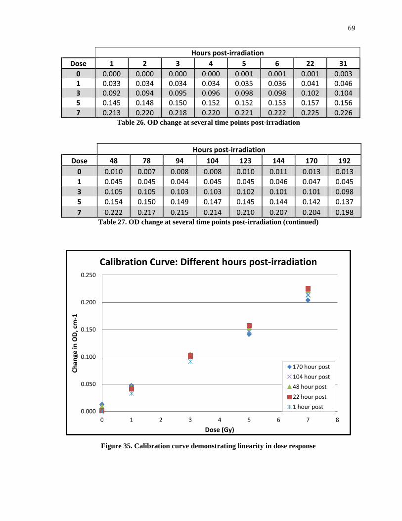
69
Hours post-irradiation
Dose 1 2 3 4 5 6 22 31
0 0.000 0.000 0.000 0.000 0.001 0.001 0.001 0.003 1 0.033 0.034 0.034 0.034 0.035 0.036 0.041 0.046 3 0.092 0.094 0.095 0.096 0.098 0.098 0.102 0.104 5 0.145 0.148 0.150 0.152 0.152 0.153 0.157 0.156
7 0.213 0.220 0.218 0.220 0.221 0.222 0.225 0.226 Table 26. OD change at several time points post-irradiation
Hours post-irradiation
Dose 48 78 94 104 123 144 170 192
0 0.010 0.007 0.008 0.008 0.010 0.011 0.013 0.013
1 0.045 0.045 0.044 0.045 0.045 0.046 0.047 0.045
3 0.105 0.105 0.103 0.103 0.102 0.101 0.101 0.098
5 0.154 0.150 0.149 0.147 0.145 0.144 0.142 0.137
7 0.222 0.217 0.215 0.214 0.210 0.207 0.204 0.198 Table 27. OD change at several time points post-irradiation (continued)
Figure 35. Calibration curve demonstrating linearity in dose response
0.000
0.050
0.100
0.150
0.200
0.250
0 1 2 3 4 5 6 7 8
Ch
ange
in O
D, c
m-1
Dose (Gy)
Calibration Curve: Different hours post-irradiation
170 hour post
104 hour post
48 hour post
22 hour post
1 hour post
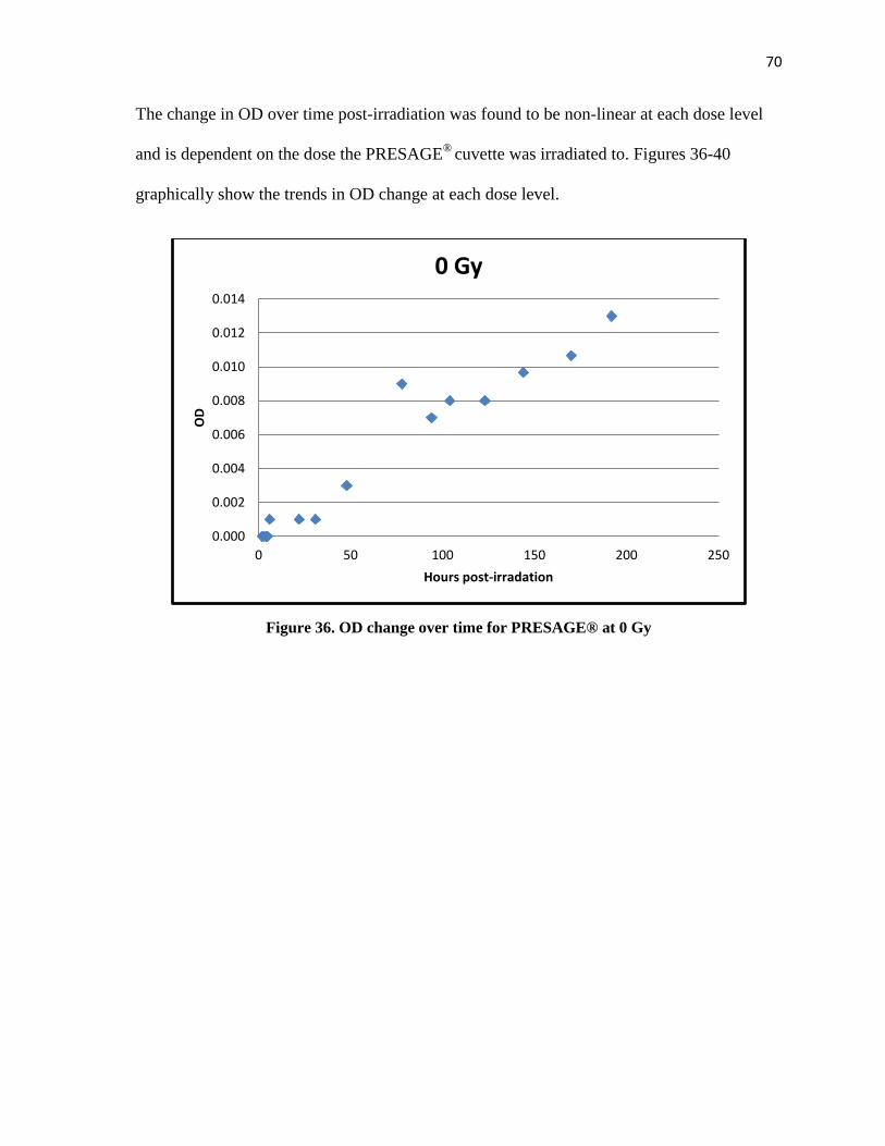
70
The change in OD over time post-irradiation was found to be non-linear at each dose level
and is dependent on the dose the PRESAGE®
cuvette was irradiated to. Figures 36-40
graphically show the trends in OD change at each dose level.
Figure 36. OD change over time for PRESAGE® at 0 Gy
0.000
0.002
0.004
0.006
0.008
0.010
0.012
0.014
0 50 100 150 200 250
OD
Hours post-irradation
0 Gy
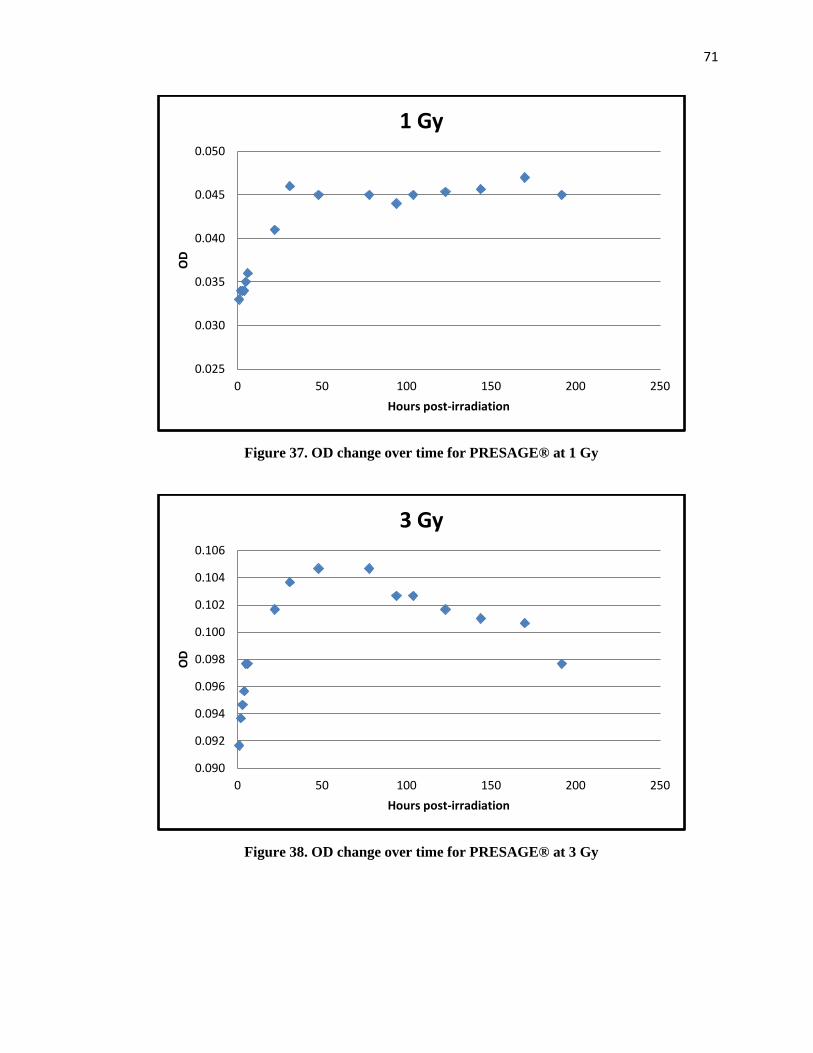
71
Figure 37. OD change over time for PRESAGE® at 1 Gy
Figure 38. OD change over time for PRESAGE® at 3 Gy
0.025
0.030
0.035
0.040
0.045
0.050
0 50 100 150 200 250
OD
Hours post-irradiation
1 Gy
0.090
0.092
0.094
0.096
0.098
0.100
0.102
0.104
0.106
0 50 100 150 200 250
OD
Hours post-irradiation
3 Gy
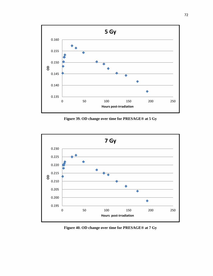
72
Figure 39. OD change over time for PRESAGE® at 5 Gy
Figure 40. OD change over time for PRESAGE® at 7 Gy
0.135
0.140
0.145
0.150
0.155
0.160
0 50 100 150 200 250
OD
Hours post-irradiation
5 Gy
0.195
0.200
0.205
0.210
0.215
0.220
0.225
0.230
0 50 100 150 200 250
OD
Hours post-irradiation
7 Gy
73
This study shows that OD changes in PRESAGE® over time can vary drastically
depending on the dose deposited in the dosimeter. With no dose deposited, the OD change in
PRESAGE® increases relatively linearly over time. This was expected, since PRESAGE
® is
known to darken at a faster rate at room temperature. For higher doses of 3 Gy, 5 Gy and 7
Gy, the OD response increases until approximately 31-50 hours post-irradiation, then
consistently decreases with time. Unexpectedly, the change in OD beyond 100 hours post-
irradiation fell below the initial OD response at 5 Gy and 7 Gy. This phenomenon of the
fading of signal at different rates for different doses in PRESAGE® suggests that the post-
irradiation optical-CT scan for dosimeters should be held within 48 hours after irradiation.
The OD response to 1 Gy continually increased until approximately 48 hours and then
maintained a relatively constant response from 48-192 hours. Since the over-response
measurements were in regions of dose levels below 1 Gy, the results at 1 Gy was the best
approximation for the dose levels at r = 4 to 5 cm in the Amersham 6711 large channel
dosimeter and r = 2.5 to 5 cm in the AgX100 large channel dosimeter.
The change in response at 1 Gy was the greatest compared to the rest of the dose
responses at higher doses. While the higher doses eventually began to decrease in response,
the response at 1 Gy did not follow the same trend. Since the irradiation times for the large
channel dosimeters ranged from approximately 5 to 10 days, the OD response to the doses
deposited within the first few days of the irradiation were likely to have changed drastically
by the time of the post-irradiation optical-CT scan. The OD at larger distances from the
source (smaller doses) did not experience the drastic decrease in OD at smaller distances
(larger doses) from the source. Therefore, after the irradiation duration of 5-10 days and the
dose values were captured and normalized to the dose at 1.5 cm, the non-linear changes over
74
the irradiation period resulted in dose values much higher than expected at the larger
distances.
Figure 44 below shows the isodose lines on the transverse bisecting plane of the
large channel dosimeter irradiated with the AgX100. The isodose lines represent the doses
expected (calculated using the dose rate constant), where the pink line represents the
calculated dose at 1.5 cm, the green represents the calculated dose at 2 cm, blue represents
the calculated dose at 3 cm, and so forth. By measuring the diameters of each isodose curve
(distances are displayed in the figure), it was determined that the expected doses at r = 3 cm,
r = 4 cm, r = 5 cm actually ended up at r = 3.07 cm, r = 4.44 cm, and r = 5.25 cm. The
isodose curves for doses at r = 1.5 cm and r = 2 cm were accurate in measurement. This
proved to be a visual confirmation of the over-response farther away from the source at
doses below 1 Gy. The jaggedness of the isodose lines beyond 2.552 Gy also suggests that
the OD response was unstable and was perhaps changing, or that the small dose values
resulted in larger statistical variations.
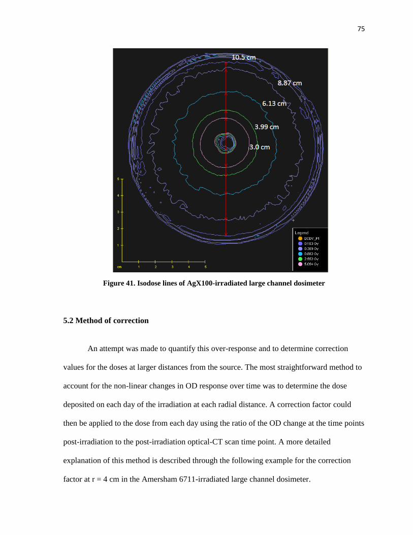
75
Figure 41. Isodose lines of AgX100-irradiated large channel dosimeter
5.2 Method of correction
An attempt was made to quantify this over-response and to determine correction
values for the doses at larger distances from the source. The most straightforward method to
account for the non-linear changes in OD response over time was to determine the dose
deposited on each day of the irradiation at each radial distance. A correction factor could
then be applied to the dose from each day using the ratio of the OD change at the time points
post-irradiation to the post-irradiation optical-CT scan time point. A more detailed
explanation of this method is described through the following example for the correction
factor at r = 4 cm in the Amersham 6711-irradiated large channel dosimeter.
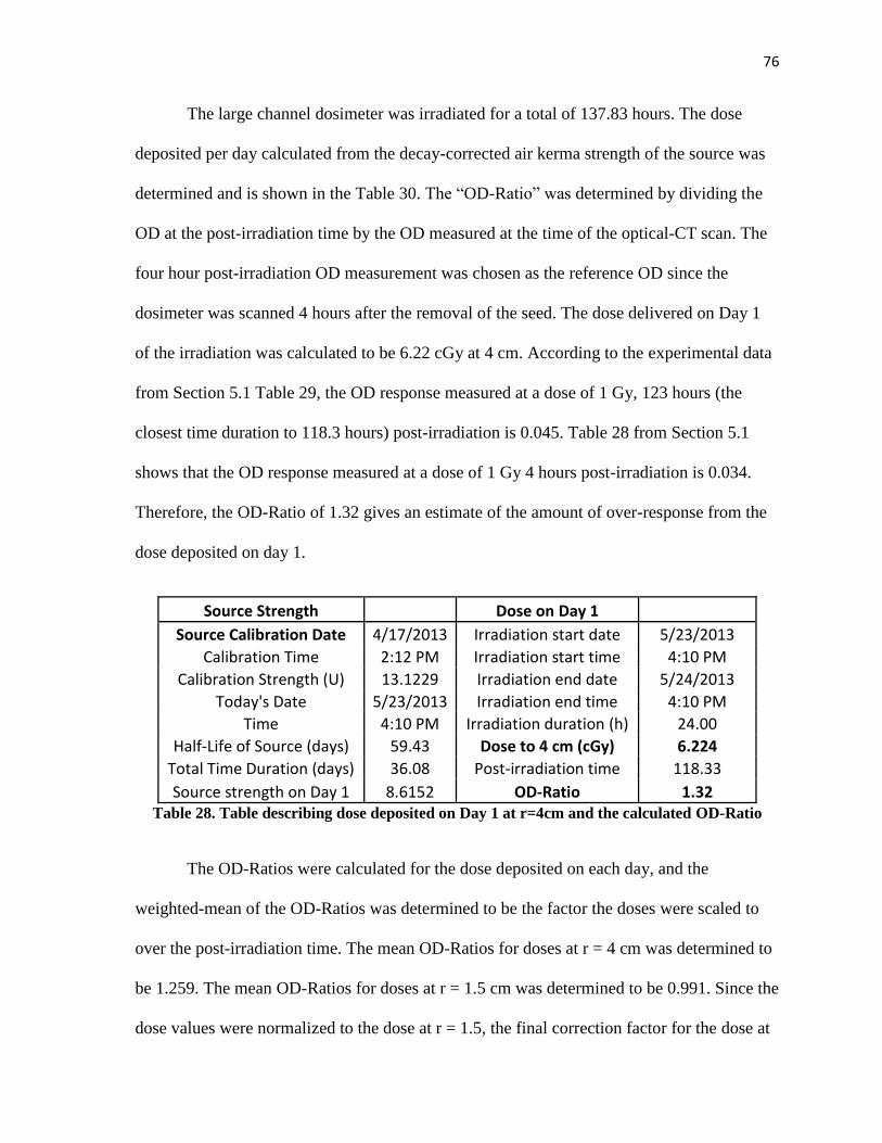
76
The large channel dosimeter was irradiated for a total of 137.83 hours. The dose
deposited per day calculated from the decay-corrected air kerma strength of the source was
determined and is shown in the Table 30. The “OD-Ratio” was determined by dividing the
OD at the post-irradiation time by the OD measured at the time of the optical-CT scan. The
four hour post-irradiation OD measurement was chosen as the reference OD since the
dosimeter was scanned 4 hours after the removal of the seed. The dose delivered on Day 1
of the irradiation was calculated to be 6.22 cGy at 4 cm. According to the experimental data
from Section 5.1 Table 29, the OD response measured at a dose of 1 Gy, 123 hours (the
closest time duration to 118.3 hours) post-irradiation is 0.045. Table 28 from Section 5.1
shows that the OD response measured at a dose of 1 Gy 4 hours post-irradiation is 0.034.
Therefore, the OD-Ratio of 1.32 gives an estimate of the amount of over-response from the
dose deposited on day 1.
Source Strength Dose on Day 1
Source Calibration Date 4/17/2013 Irradiation start date 5/23/2013
Calibration Time 2:12 PM Irradiation start time 4:10 PM
Calibration Strength (U) 13.1229 Irradiation end date 5/24/2013
Today's Date 5/23/2013 Irradiation end time 4:10 PM
Time 4:10 PM Irradiation duration (h) 24.00
Half-Life of Source (days) 59.43 Dose to 4 cm (cGy) 6.224
Total Time Duration (days) 36.08 Post-irradiation time 118.33
Source strength on Day 1 8.6152 OD-Ratio 1.32 Table 28. Table describing dose deposited on Day 1 at r=4cm and the calculated OD-Ratio
The OD-Ratios were calculated for the dose deposited on each day, and the
weighted-mean of the OD-Ratios was determined to be the factor the doses were scaled to
over the post-irradiation time. The mean OD-Ratios for doses at r = 4 cm was determined to
be 1.259. The mean OD-Ratios for doses at r = 1.5 cm was determined to be 0.991. Since the
dose values were normalized to the dose at r = 1.5, the final correction factor for the dose at
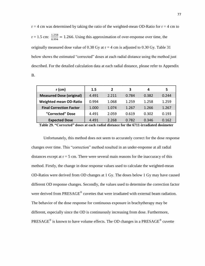
77
r = 4 cm was determined by taking the ratio of the weighted-mean OD-Ratio for r = 4 cm to
r = 1.5 cm:
. Using this approximation of over-response over time, the
originally measured dose value of 0.38 Gy at r = 4 cm is adjusted to 0.30 Gy. Table 31
below shows the estimated “corrected” doses at each radial distance using the method just
described. For the detailed calculation data at each radial distance, please refer to Appendix
B.
r (cm) 1.5 2 3 4 5
Measured Dose (original) 4.491 2.211 0.784 0.382 0.244
Weighted mean OD-Ratio 0.994 1.068 1.259 1.258 1.259
Final Correction Factor 1.000 1.074 1.267 1.266 1.267
"Corrected" Dose 4.491 2.059 0.619 0.302 0.193
Expected Dose 4.491 2.268 0.782 0.346 0.162 Table 29. “Corrected” doses at each radial distance for the 6711-irradiated dosimeter
Unfortunately, this method does not seem to accurately correct for the dose response
changes over time. This “correction” method resulted in an under-response at all radial
distances except at r = 5 cm. There were several main reasons for the inaccuracy of this
method. Firstly, the change in dose response values used to calculate the weighted-mean
OD-Ratios were derived from OD changes at 1 Gy. The doses below 1 Gy may have caused
different OD response changes. Secondly, the values used to determine the correction factor
were derived from PRESAGE® cuvettes that were irradiated with external beam radiation.
The behavior of the dose response for continuous exposure in brachytherapy may be
different, especially since the OD is continuously increasing from dose. Furthermore,
PRESAGE® is known to have volume effects. The OD changes in a PRESAGE
® cuvette
78
may not accurately represent the changes that would be observed in a large volume
PRESAGE®.
6 Uncertainty Analysis
6.1 Uncertainty in the Dose Rate Constant
As recommended by TG-43U1, the uncertainty in the brachytherapy dosimetry in
PRESAGE® dosimeters was thoroughly evaluated. The uncertainty analysis follows the
recommended protocol set forth in AAPM TG-138[15]. The summary of the Type A and
Type B uncertainties for the Amersham 6711 and the AgX100 dose measurements are listed
in Table 32 with the final estimation of the total expanded uncertainty (k=2) for a 95%
confidence limit. The total standard uncertainty (k=1) for the dose rates measured in
PRESAGE® was estimated to be 3.0% and the expanded uncertainty (k=2) was 6.0%.
Type A uncertainties in this project were the statistical uncertainties of repeated
point-dose measurements in PRESAGE®
. This uncertainty was analyzed through multiple
measurements of the same dose line profile on one plane in the dose cube. The uncertainty
was estimated to be 0.3% (k=1). The type B uncertainties in this study include several
factors. The seed calibration of each source used in this project was calibrated by the ADCL
at M.D. Anderson Cancer Center. The uncertainties in the source strength calibration include
the NIST WAFAC calibration uncertainty, the ADCL chamber calibration, and the
reproducibility of the ADCL air kerma strength measurements of the sources. The total
uncertainty was estimated to be 0.9% (k=1), as listed in Table 32. The uncertainty in the
OD-to-dose conversion lies in the fitting of the dose calibration curve and was estimated to
be 0.3%.
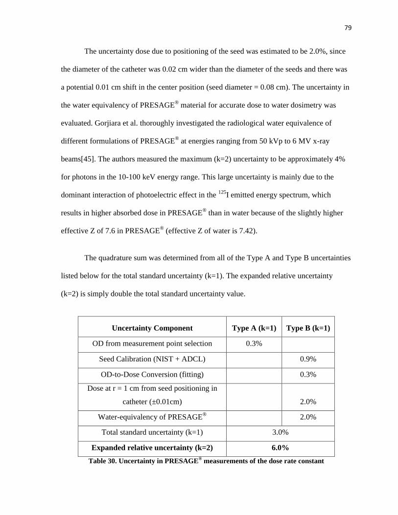
79
The uncertainty dose due to positioning of the seed was estimated to be 2.0%, since
the diameter of the catheter was 0.02 cm wider than the diameter of the seeds and there was
a potential 0.01 cm shift in the center position (seed diameter = 0.08 cm). The uncertainty in
the water equivalency of PRESAGE® material for accurate dose to water dosimetry was
evaluated. Gorjiara et al. thoroughly investigated the radiological water equivalence of
different formulations of PRESAGE® at energies ranging from 50 kVp to 6 MV x-ray
beams[45]. The authors measured the maximum (k=2) uncertainty to be approximately 4%
for photons in the 10-100 keV energy range. This large uncertainty is mainly due to the
dominant interaction of photoelectric effect in the 125
I emitted energy spectrum, which
results in higher absorbed dose in PRESAGE® than in water because of the slightly higher
effective Z of 7.6 in PRESAGE® (effective Z of water is 7.42).
The quadrature sum was determined from all of the Type A and Type B uncertainties
listed below for the total standard uncertainty (k=1). The expanded relative uncertainty
(k=2) is simply double the total standard uncertainty value.
Uncertainty Component Type A (k=1) Type B (k=1)
OD from measurement point selection 0.3%
Seed Calibration (NIST + ADCL) 0.9%
OD-to-Dose Conversion (fitting) 0.3%
Dose at r = 1 cm from seed positioning in
catheter (±0.01cm) 2.0%
Water-equivalency of PRESAGE®
2.0%
Total standard uncertainty (k=1) 3.0%
Expanded relative uncertainty (k=2) 6.0%
Table 30. Uncertainty in PRESAGE® measurements of the dose rate constant
80
6.2 Uncertainty in Anisotropy Function
By definition, anisotropy is a ratio between two doses. As such, error (uncertainty) in
seed calibration and uncertainty due to water equivalency would cancel out. Source
positioning uncertainty (±0.01 cm) would also have somewhat compensatory effects for
anisotropy calculation. The resulting uncertainty from source positioning was estimated to
be 1.0%. Therefore, resulting dose uncertainty for anisotropy would reduce to 1.1%. Thus,
uncertainty (k=1) in measured anisotropy values would be 1.5%. The expanded relative
uncertainty (k=2) would be 3.0%.
6.3 Uncertainty in the Radial Dose Function
Like anisotropy, radial dose function values are ratios of two doses. Therefore, the
uncertainty arguments stated for dose anisotropy would apply for radial dose function as
well. However, source position uncertainty (±0.01 cm) may have a higher impact at shorter
radial distances. The uncertainty (k=1) in measured radial dose values would be 1.5% and
the expanded relative uncertainty (k=2) would be 3.0%.
7 Conclusion
The hypothesis for this project was accepted for dose measurements up to r=3 cm.
The dosimetric parameters measured in PRESAGE® using the Amersham 6711 seed model
were within ±5% of the TG-43U1 values for dosimetry parameters measured in the range of
r = 1 to r = 3 cm. The AgX100 seed model was successfully characterized using
PRESAGE® from r = 1 to r = 3 cm.
81
The results of this study demonstrate great potential in use of PRESAGE® for
brachytherapy dosimetry. For both the Amersham 6711 and AgX100 seed irradiations, the
measured dose rates up to distances 3 cm away from the source were within ±3% of the
consensus values. The radial functions and the anisotropy functions measured in
PRESAGE® also agreed well with values in TG-43U1 and previous publications. The
AgX100 seed was successfully characterized, and the resulting dosimetric parameters agreed
with Monte Carlo derived values within ±9%.
However, there are several factors to be aware of for future work. First of all, the
issue with the rate of OD change with time in different dose ranges needs to be addressed for
more accurate dosimetry in the future. This can be done either by using high air kerma
strength sources to keep irradiation times low and dose values high, or by finding a way to
correct for the dose response changes. As shown in Chapter 5, finding an appropriate
method to accurately correct for the OD change at different doses over different post-
irradiation time periods can be a difficult and complicated task. To avoid dealing with this
phenomenon in PRESAGE®, it would be best to keep the time between seed placement in
the dosimeter to the post-irradiation optical-CT scan within 48 hours. Secondly, the doses
used for dosimetry measurements should be at a minimum of 20 cGy. For a coefficient of
variation under 3%, doses should be at a minimum of 1 Gy.
As with every research project, there is always much room for improvements. To
continue with this work, it would be strongly beneficial for a more advanced method of dose
analysis. The dose measurements in this project were acquired manually through dose line
profiles in CERR and the calculated dosimetric parameters were computationally intensive
82
and time-consuming. A more automatic method of analysis- perhaps similar to a 3D gamma
analysis- would be more efficient. Furthermore, the effective Z of PRESAGE® is water-
equivalent for MV energy radiation beams. Although the PRESAGE® formulations are
continuously improving and the effective Z of the O-MeO-LMG formulation used in this
study is even lower than the effective Z of the formulations previously evaluated by Gorjiara
et al., it is possible that a small correction factor may still needed for the low energy emitted
by 125I sources.
The findings in this study help to pave the way for 3D brachytherapy dosimetry in
PRESAGE®, which would greatly improve the general knowledge and confidence in the 3D
dosimetry of sources used in brachytherapy and also advance quality assurance methods.
Despite the limitations described previously, PRESAGE® can serve as a reliable dosimetry
tool, especially for high activity irradiations. Future work in dosimetry evaluations for HDR
devices or the COMS eye plaque (consisting of multiple seeds for a higher total activity) in
PRESAGE® are likely to produce promising results and may be the start of the new 3D
dosimetry era for brachytherapy.
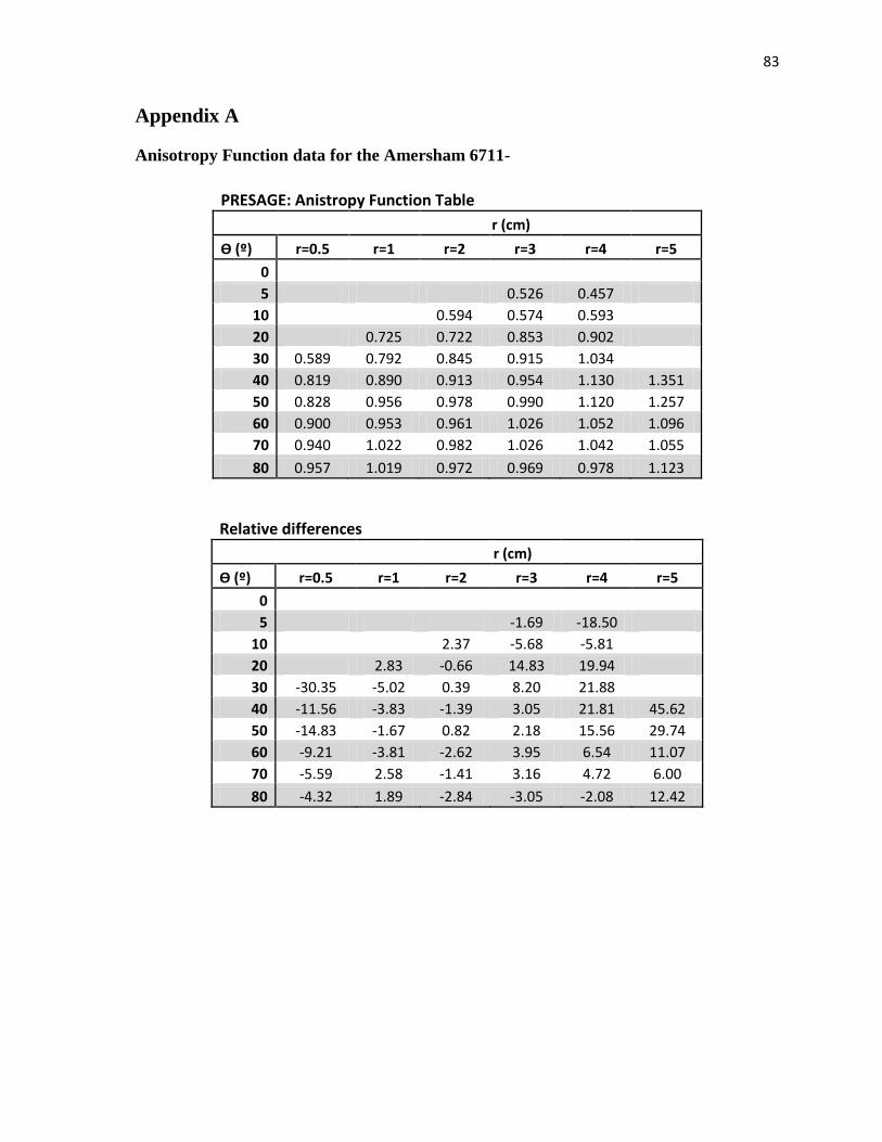
83
Appendix A
Anisotropy Function data for the Amersham 6711-
PRESAGE: Anistropy Function Table r (cm)
Ѳ (º) r=0.5 r=1 r=2 r=3 r=4 r=5
0
5 0.526 0.457
10
0.594 0.574 0.593
20 0.725 0.722 0.853 0.902
30 0.589 0.792 0.845 0.915 1.034
40 0.819 0.890 0.913 0.954 1.130 1.351
50 0.828 0.956 0.978 0.990 1.120 1.257
60 0.900 0.953 0.961 1.026 1.052 1.096
70 0.940 1.022 0.982 1.026 1.042 1.055
80 0.957 1.019 0.972 0.969 0.978 1.123
Relative differences r (cm)
Ѳ (º) r=0.5 r=1 r=2 r=3 r=4 r=5
0
5 -1.69 -18.50
10
2.37 -5.68 -5.81
20 2.83 -0.66 14.83 19.94
30 -30.35 -5.02 0.39 8.20 21.88
40 -11.56 -3.83 -1.39 3.05 21.81 45.62
50 -14.83 -1.67 0.82 2.18 15.56 29.74
60 -9.21 -3.81 -2.62 3.95 6.54 11.07
70 -5.59 2.58 -1.41 3.16 4.72 6.00
80 -4.32 1.89 -2.84 -3.05 -2.08 12.42
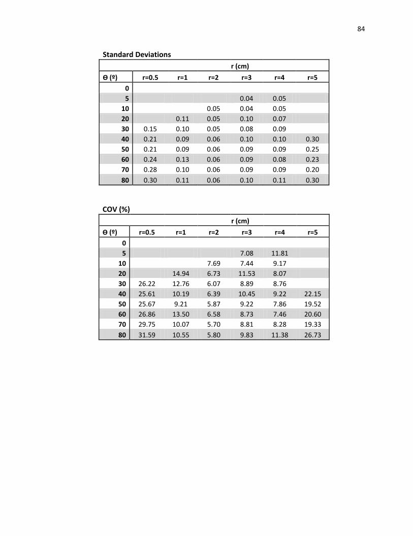
84
Standard Deviations r (cm)
Ѳ (º) r=0.5 r=1 r=2 r=3 r=4 r=5
0
5 0.04 0.05
10
0.05 0.04 0.05
20 0.11 0.05 0.10 0.07
30 0.15 0.10 0.05 0.08 0.09
40 0.21 0.09 0.06 0.10 0.10 0.30
50 0.21 0.09 0.06 0.09 0.09 0.25
60 0.24 0.13 0.06 0.09 0.08 0.23
70 0.28 0.10 0.06 0.09 0.09 0.20
80 0.30 0.11 0.06 0.10 0.11 0.30
COV (%) r (cm)
Ѳ (º) r=0.5 r=1 r=2 r=3 r=4 r=5
0
5 7.08 11.81
10
7.69 7.44 9.17
20 14.94 6.73 11.53 8.07
30 26.22 12.76 6.07 8.89 8.76
40 25.61 10.19 6.39 10.45 9.22 22.15
50 25.67 9.21 5.87 9.22 7.86 19.52
60 26.86 13.50 6.58 8.73 7.46 20.60
70 29.75 10.07 5.70 8.81 8.28 19.33
80 31.59 10.55 5.80 9.83 11.38 26.73
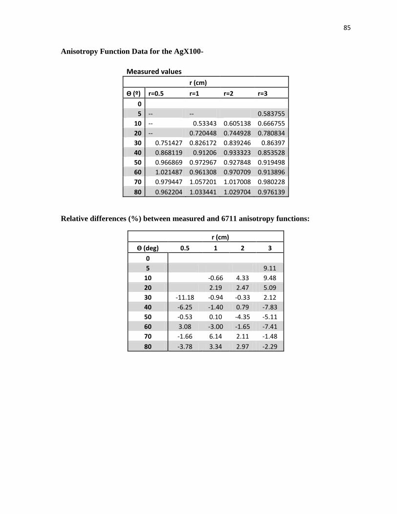
85
Anisotropy Function Data for the AgX100-
Measured values r (cm)
Ѳ (º) r=0.5 r=1 r=2 r=3
0
5 -- -- 0.583755
10 -- 0.53343 0.605138 0.666755
20 -- 0.720448 0.744928 0.780834
30 0.751427 0.826172 0.839246 0.86397
40 0.868119 0.91206 0.933323 0.853528
50 0.966869 0.972967 0.927848 0.919498
60 1.021487 0.961308 0.970709 0.913896
70 0.979447 1.057201 1.017008 0.980228
80 0.962204 1.033441 1.029704 0.976139
Relative differences (%) between measured and 6711 anisotropy functions:
r (cm)
Ѳ (deg) 0.5 1 2 3
0
5 9.11
10 -0.66 4.33 9.48
20 2.19 2.47 5.09
30 -11.18 -0.94 -0.33 2.12
40 -6.25 -1.40 0.79 -7.83
50 -0.53 0.10 -4.35 -5.11
60 3.08 -3.00 -1.65 -7.41
70 -1.66 6.14 2.11 -1.48
80 -3.78 3.34 2.97 -2.29
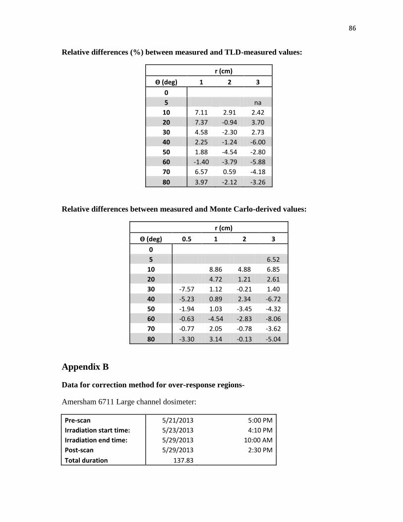
86
Relative differences (%) between measured and TLD-measured values:
r (cm)
Ѳ (deg) 1 2 3
0
5 na
10 7.11 2.91 2.42
20 7.37 -0.94 3.70
30 4.58 -2.30 2.73
40 2.25 -1.24 -6.00
50 1.88 -4.54 -2.80
60 -1.40 -3.79 -5.88
70 6.57 0.59 -4.18
80 3.97 -2.12 -3.26
Relative differences between measured and Monte Carlo-derived values:
r (cm)
Ѳ (deg) 0.5 1 2 3
0
5 6.52
10 8.86 4.88 6.85
20 4.72 1.21 2.61
30 -7.57 1.12 -0.21 1.40
40 -5.23 0.89 2.34 -6.72
50 -1.94 1.03 -3.45 -4.32
60 -0.63 -4.54 -2.83 -8.06
70 -0.77 2.05 -0.78 -3.62
80 -3.30 3.14 -0.13 -5.04
Appendix B
Data for correction method for over-response regions-
Amersham 6711 Large channel dosimeter:
Pre-scan 5/21/2013 5:00 PM
Irradiation start time: 5/23/2013 4:10 PM
Irradiation end time: 5/29/2013 10:00 AM
Post-scan 5/29/2013 2:30 PM
Total duration 137.83
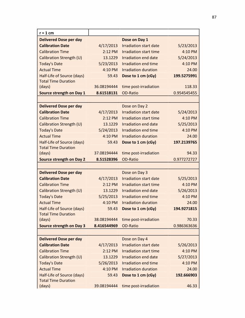
87
r = 1 cm
Delivered Dose per day Dose on Day 1
Calibration Date 4/17/2013 Irradiation start date 5/23/2013
Calibration Time 2:12 PM Irradiation start time 4:10 PM
Calibration Strength (U) 13.1229 Irradiation end date 5/24/2013
Today's Date 5/23/2013 Irradiation end time 4:10 PM
Actual Time 4:10 PM Irradiation duration 24.00
Half-Life of Source (days) 59.43 Dose to 1 cm (cGy) 199.5275991 Total Time Duration (days) 36.08194444 time post-irradiation 118.33
Source strength on Day 1 8.61518131 OD-Ratio 0.954545455
Delivered Dose per day Dose on Day 2
Calibration Date 4/17/2013 Irradiation start date 5/24/2013
Calibration Time 2:12 PM Irradiation start time 4:10 PM
Calibration Strength (U) 13.1229 Irradiation end date 5/25/2013
Today's Date 5/24/2013 Irradiation end time 4:10 PM
Actual Time 4:10 PM Irradiation duration 24.00
Half-Life of Source (days) 59.43 Dose to 1 cm (cGy) 197.2139765 Total Time Duration (days) 37.08194444 time post-irradiation 94.33
Source strength on Day 2 8.51528396 OD-Ratio 0.977272727
Delivered Dose per day Dose on Day 3
Calibration Date 4/17/2013 Irradiation start date 5/25/2013
Calibration Time 2:12 PM Irradiation start time 4:10 PM
Calibration Strength (U) 13.1229 Irradiation end date 5/26/2013
Today's Date 5/25/2013 Irradiation end time 4:10 PM
Actual Time 4:10 PM Irradiation duration 24.00
Half-Life of Source (days) 59.43 Dose to 1 cm (cGy) 194.9271815 Total Time Duration (days) 38.08194444 time post-irradiation 70.33
Source strength on Day 3 8.416544969 OD-Ratio 0.986363636
Delivered Dose per day Dose on Day 4
Calibration Date 4/17/2013 Irradiation start date 5/26/2013
Calibration Time 2:12 PM Irradiation start time 4:10 PM
Calibration Strength (U) 13.1229 Irradiation end date 5/27/2013
Today's Date 5/26/2013 Irradiation end time 4:10 PM
Actual Time 4:10 PM Irradiation duration 24.00
Half-Life of Source (days) 59.43 Dose to 1 cm (cGy) 192.666903 Total Time Duration (days) 39.08194444 time post-irradiation 46.33
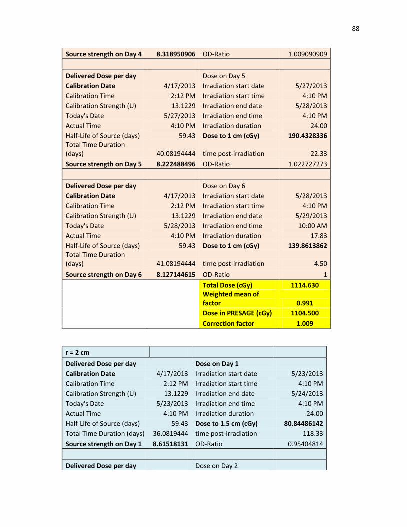
88
Source strength on Day 4 8.318950906 OD-Ratio 1.009090909
Delivered Dose per day Dose on Day 5
Calibration Date 4/17/2013 Irradiation start date 5/27/2013
Calibration Time 2:12 PM Irradiation start time 4:10 PM
Calibration Strength (U) 13.1229 Irradiation end date 5/28/2013
Today's Date 5/27/2013 Irradiation end time 4:10 PM
Actual Time 4:10 PM Irradiation duration 24.00
Half-Life of Source (days) 59.43 Dose to 1 cm (cGy) 190.4328336 Total Time Duration (days) 40.08194444 time post-irradiation 22.33
Source strength on Day 5 8.222488496 OD-Ratio 1.022727273
Delivered Dose per day Dose on Day 6
Calibration Date 4/17/2013 Irradiation start date 5/28/2013
Calibration Time 2:12 PM Irradiation start time 4:10 PM
Calibration Strength (U) 13.1229 Irradiation end date 5/29/2013
Today's Date 5/28/2013 Irradiation end time 10:00 AM
Actual Time 4:10 PM Irradiation duration 17.83
Half-Life of Source (days) 59.43 Dose to 1 cm (cGy) 139.8613862 Total Time Duration (days) 41.08194444 time post-irradiation 4.50
Source strength on Day 6 8.127144615 OD-Ratio 1
Total Dose (cGy) 1114.630
Weighted mean of factor 0.991
Dose in PRESAGE (cGy) 1104.500
Correction factor 1.009
r = 2 cm
Delivered Dose per day Dose on Day 1
Calibration Date 4/17/2013 Irradiation start date 5/23/2013
Calibration Time 2:12 PM Irradiation start time 4:10 PM
Calibration Strength (U) 13.1229 Irradiation end date 5/24/2013
Today's Date 5/23/2013 Irradiation end time 4:10 PM
Actual Time 4:10 PM Irradiation duration 24.00
Half-Life of Source (days) 59.43 Dose to 1.5 cm (cGy) 80.84486142
Total Time Duration (days) 36.0819444 time post-irradiation 118.33
Source strength on Day 1 8.61518131 OD-Ratio 0.95404814
Delivered Dose per day Dose on Day 2
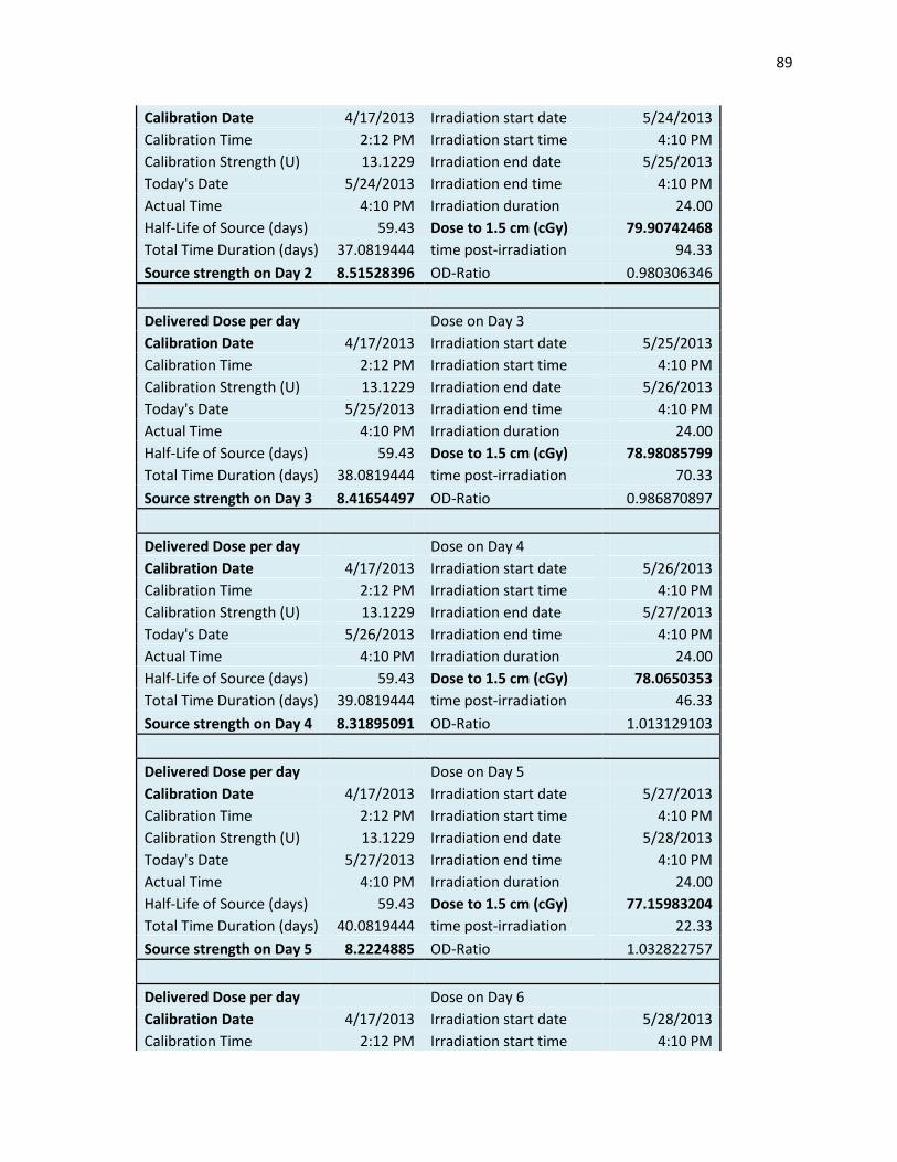
89
Calibration Date 4/17/2013 Irradiation start date 5/24/2013
Calibration Time 2:12 PM Irradiation start time 4:10 PM
Calibration Strength (U) 13.1229 Irradiation end date 5/25/2013
Today's Date 5/24/2013 Irradiation end time 4:10 PM
Actual Time 4:10 PM Irradiation duration 24.00
Half-Life of Source (days) 59.43 Dose to 1.5 cm (cGy) 79.90742468
Total Time Duration (days) 37.0819444 time post-irradiation 94.33
Source strength on Day 2 8.51528396 OD-Ratio 0.980306346
Delivered Dose per day Dose on Day 3
Calibration Date 4/17/2013 Irradiation start date 5/25/2013
Calibration Time 2:12 PM Irradiation start time 4:10 PM
Calibration Strength (U) 13.1229 Irradiation end date 5/26/2013
Today's Date 5/25/2013 Irradiation end time 4:10 PM
Actual Time 4:10 PM Irradiation duration 24.00
Half-Life of Source (days) 59.43 Dose to 1.5 cm (cGy) 78.98085799
Total Time Duration (days) 38.0819444 time post-irradiation 70.33
Source strength on Day 3 8.41654497 OD-Ratio 0.986870897
Delivered Dose per day Dose on Day 4
Calibration Date 4/17/2013 Irradiation start date 5/26/2013
Calibration Time 2:12 PM Irradiation start time 4:10 PM
Calibration Strength (U) 13.1229 Irradiation end date 5/27/2013
Today's Date 5/26/2013 Irradiation end time 4:10 PM
Actual Time 4:10 PM Irradiation duration 24.00
Half-Life of Source (days) 59.43 Dose to 1.5 cm (cGy) 78.0650353
Total Time Duration (days) 39.0819444 time post-irradiation 46.33
Source strength on Day 4 8.31895091 OD-Ratio 1.013129103
Delivered Dose per day Dose on Day 5
Calibration Date 4/17/2013 Irradiation start date 5/27/2013
Calibration Time 2:12 PM Irradiation start time 4:10 PM
Calibration Strength (U) 13.1229 Irradiation end date 5/28/2013
Today's Date 5/27/2013 Irradiation end time 4:10 PM
Actual Time 4:10 PM Irradiation duration 24.00
Half-Life of Source (days) 59.43 Dose to 1.5 cm (cGy) 77.15983204
Total Time Duration (days) 40.0819444 time post-irradiation 22.33
Source strength on Day 5 8.2224885 OD-Ratio 1.032822757
Delivered Dose per day Dose on Day 6
Calibration Date 4/17/2013 Irradiation start date 5/28/2013
Calibration Time 2:12 PM Irradiation start time 4:10 PM
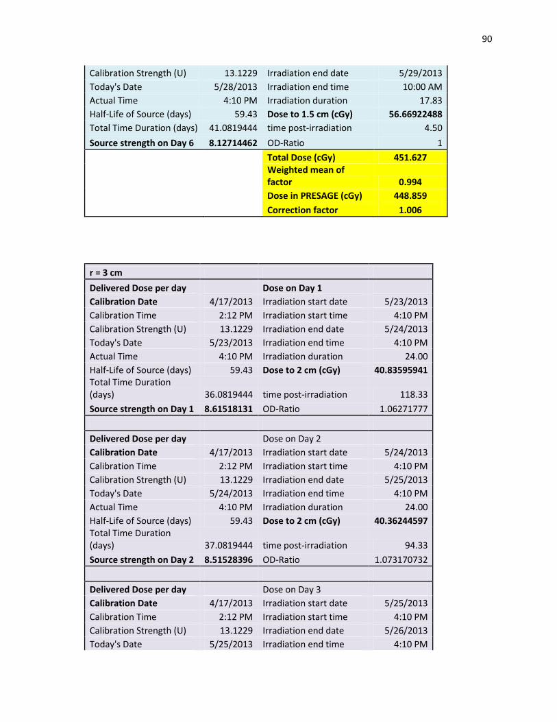
90
Calibration Strength (U) 13.1229 Irradiation end date 5/29/2013
Today's Date 5/28/2013 Irradiation end time 10:00 AM
Actual Time 4:10 PM Irradiation duration 17.83
Half-Life of Source (days) 59.43 Dose to 1.5 cm (cGy) 56.66922488
Total Time Duration (days) 41.0819444 time post-irradiation 4.50
Source strength on Day 6 8.12714462 OD-Ratio 1
Total Dose (cGy) 451.627
Weighted mean of factor 0.994
Dose in PRESAGE (cGy) 448.859
Correction factor 1.006
r = 3 cm
Delivered Dose per day Dose on Day 1
Calibration Date 4/17/2013 Irradiation start date 5/23/2013
Calibration Time 2:12 PM Irradiation start time 4:10 PM
Calibration Strength (U) 13.1229 Irradiation end date 5/24/2013
Today's Date 5/23/2013 Irradiation end time 4:10 PM
Actual Time 4:10 PM Irradiation duration 24.00
Half-Life of Source (days) 59.43 Dose to 2 cm (cGy) 40.83595941 Total Time Duration (days) 36.0819444 time post-irradiation 118.33
Source strength on Day 1 8.61518131 OD-Ratio 1.06271777
Delivered Dose per day Dose on Day 2
Calibration Date 4/17/2013 Irradiation start date 5/24/2013
Calibration Time 2:12 PM Irradiation start time 4:10 PM
Calibration Strength (U) 13.1229 Irradiation end date 5/25/2013
Today's Date 5/24/2013 Irradiation end time 4:10 PM
Actual Time 4:10 PM Irradiation duration 24.00
Half-Life of Source (days) 59.43 Dose to 2 cm (cGy) 40.36244597 Total Time Duration (days) 37.0819444 time post-irradiation 94.33
Source strength on Day 2 8.51528396 OD-Ratio 1.073170732
Delivered Dose per day Dose on Day 3
Calibration Date 4/17/2013 Irradiation start date 5/25/2013
Calibration Time 2:12 PM Irradiation start time 4:10 PM
Calibration Strength (U) 13.1229 Irradiation end date 5/26/2013
Today's Date 5/25/2013 Irradiation end time 4:10 PM
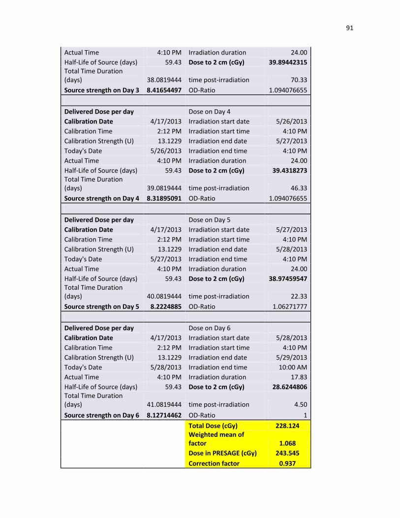
91
Actual Time 4:10 PM Irradiation duration 24.00
Half-Life of Source (days) 59.43 Dose to 2 cm (cGy) 39.89442315 Total Time Duration (days) 38.0819444 time post-irradiation 70.33
Source strength on Day 3 8.41654497 OD-Ratio 1.094076655
Delivered Dose per day Dose on Day 4
Calibration Date 4/17/2013 Irradiation start date 5/26/2013
Calibration Time 2:12 PM Irradiation start time 4:10 PM
Calibration Strength (U) 13.1229 Irradiation end date 5/27/2013
Today's Date 5/26/2013 Irradiation end time 4:10 PM
Actual Time 4:10 PM Irradiation duration 24.00
Half-Life of Source (days) 59.43 Dose to 2 cm (cGy) 39.4318273 Total Time Duration (days) 39.0819444 time post-irradiation 46.33
Source strength on Day 4 8.31895091 OD-Ratio 1.094076655
Delivered Dose per day Dose on Day 5
Calibration Date 4/17/2013 Irradiation start date 5/27/2013
Calibration Time 2:12 PM Irradiation start time 4:10 PM
Calibration Strength (U) 13.1229 Irradiation end date 5/28/2013
Today's Date 5/27/2013 Irradiation end time 4:10 PM
Actual Time 4:10 PM Irradiation duration 24.00
Half-Life of Source (days) 59.43 Dose to 2 cm (cGy) 38.97459547 Total Time Duration (days) 40.0819444 time post-irradiation 22.33
Source strength on Day 5 8.2224885 OD-Ratio 1.06271777
Delivered Dose per day Dose on Day 6
Calibration Date 4/17/2013 Irradiation start date 5/28/2013
Calibration Time 2:12 PM Irradiation start time 4:10 PM
Calibration Strength (U) 13.1229 Irradiation end date 5/29/2013
Today's Date 5/28/2013 Irradiation end time 10:00 AM
Actual Time 4:10 PM Irradiation duration 17.83
Half-Life of Source (days) 59.43 Dose to 2 cm (cGy) 28.6244806 Total Time Duration (days) 41.0819444 time post-irradiation 4.50
Source strength on Day 6 8.12714462 OD-Ratio 1
Total Dose (cGy) 228.124
Weighted mean of factor 1.068
Dose in PRESAGE (cGy) 243.545
Correction factor 0.937
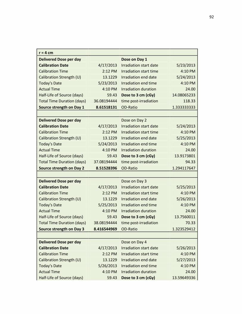
92
r = 4 cm
Delivered Dose per day Dose on Day 1
Calibration Date 4/17/2013 Irradiation start date 5/23/2013
Calibration Time 2:12 PM Irradiation start time 4:10 PM
Calibration Strength (U) 13.1229 Irradiation end date 5/24/2013
Today's Date 5/23/2013 Irradiation end time 4:10 PM
Actual Time 4:10 PM Irradiation duration 24.00
Half-Life of Source (days) 59.43 Dose to 3 cm (cGy) 14.08065233
Total Time Duration (days) 36.08194444 time post-irradiation 118.33
Source strength on Day 1 8.61518131 OD-Ratio 1.333333333
Delivered Dose per day Dose on Day 2
Calibration Date 4/17/2013 Irradiation start date 5/24/2013
Calibration Time 2:12 PM Irradiation start time 4:10 PM
Calibration Strength (U) 13.1229 Irradiation end date 5/25/2013
Today's Date 5/24/2013 Irradiation end time 4:10 PM
Actual Time 4:10 PM Irradiation duration 24.00
Half-Life of Source (days) 59.43 Dose to 3 cm (cGy) 13.9173801
Total Time Duration (days) 37.08194444 time post-irradiation 94.33
Source strength on Day 2 8.51528396 OD-Ratio 1.294117647
Delivered Dose per day Dose on Day 3
Calibration Date 4/17/2013 Irradiation start date 5/25/2013
Calibration Time 2:12 PM Irradiation start time 4:10 PM
Calibration Strength (U) 13.1229 Irradiation end date 5/26/2013
Today's Date 5/25/2013 Irradiation end time 4:10 PM
Actual Time 4:10 PM Irradiation duration 24.00
Half-Life of Source (days) 59.43 Dose to 3 cm (cGy) 13.7560011
Total Time Duration (days) 38.08194444 time post-irradiation 70.33
Source strength on Day 3 8.416544969 OD-Ratio 1.323529412
Delivered Dose per day Dose on Day 4
Calibration Date 4/17/2013 Irradiation start date 5/26/2013
Calibration Time 2:12 PM Irradiation start time 4:10 PM
Calibration Strength (U) 13.1229 Irradiation end date 5/27/2013
Today's Date 5/26/2013 Irradiation end time 4:10 PM
Actual Time 4:10 PM Irradiation duration 24.00
Half-Life of Source (days) 59.43 Dose to 3 cm (cGy) 13.59649336
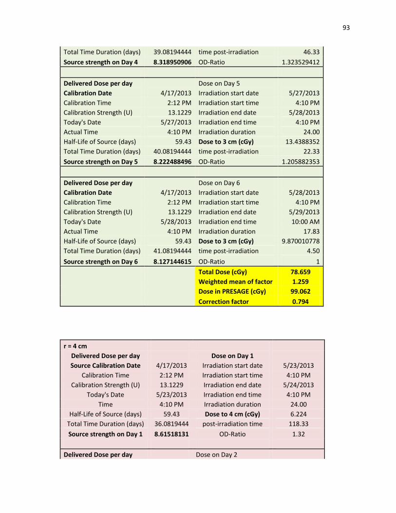
93
Total Time Duration (days) 39.08194444 time post-irradiation 46.33
Source strength on Day 4 8.318950906 OD-Ratio 1.323529412
Delivered Dose per day Dose on Day 5
Calibration Date 4/17/2013 Irradiation start date 5/27/2013
Calibration Time 2:12 PM Irradiation start time 4:10 PM
Calibration Strength (U) 13.1229 Irradiation end date 5/28/2013
Today's Date 5/27/2013 Irradiation end time 4:10 PM
Actual Time 4:10 PM Irradiation duration 24.00
Half-Life of Source (days) 59.43 Dose to 3 cm (cGy) 13.4388352
Total Time Duration (days) 40.08194444 time post-irradiation 22.33
Source strength on Day 5 8.222488496 OD-Ratio 1.205882353
Delivered Dose per day Dose on Day 6
Calibration Date 4/17/2013 Irradiation start date 5/28/2013
Calibration Time 2:12 PM Irradiation start time 4:10 PM
Calibration Strength (U) 13.1229 Irradiation end date 5/29/2013
Today's Date 5/28/2013 Irradiation end time 10:00 AM
Actual Time 4:10 PM Irradiation duration 17.83
Half-Life of Source (days) 59.43 Dose to 3 cm (cGy) 9.870010778
Total Time Duration (days) 41.08194444 time post-irradiation 4.50
Source strength on Day 6 8.127144615 OD-Ratio 1
Total Dose (cGy) 78.659
Weighted mean of factor 1.259
Dose in PRESAGE (cGy) 99.062
Correction factor 0.794
r = 4 cm
Delivered Dose per day Dose on Day 1
Source Calibration Date 4/17/2013 Irradiation start date 5/23/2013
Calibration Time 2:12 PM Irradiation start time 4:10 PM
Calibration Strength (U) 13.1229 Irradiation end date 5/24/2013
Today's Date 5/23/2013 Irradiation end time 4:10 PM
Time 4:10 PM Irradiation duration 24.00
Half-Life of Source (days) 59.43 Dose to 4 cm (cGy) 6.224
Total Time Duration (days) 36.0819444 post-irradiation time 118.33
Source strength on Day 1 8.61518131 OD-Ratio 1.32
Delivered Dose per day Dose on Day 2
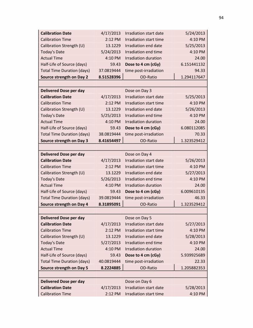
94
Calibration Date 4/17/2013 Irradiation start date 5/24/2013
Calibration Time 2:12 PM Irradiation start time 4:10 PM
Calibration Strength (U) 13.1229 Irradiation end date 5/25/2013
Today's Date 5/24/2013 Irradiation end time 4:10 PM
Actual Time 4:10 PM Irradiation duration 24.00
Half-Life of Source (days) 59.43 Dose to 4 cm (cGy) 6.151441132
Total Time Duration (days) 37.0819444 time post-irradiation 94.33
Source strength on Day 2 8.51528396 OD-Ratio 1.294117647
Delivered Dose per day Dose on Day 3
Calibration Date 4/17/2013 Irradiation start date 5/25/2013
Calibration Time 2:12 PM Irradiation start time 4:10 PM
Calibration Strength (U) 13.1229 Irradiation end date 5/26/2013
Today's Date 5/25/2013 Irradiation end time 4:10 PM
Actual Time 4:10 PM Irradiation duration 24.00
Half-Life of Source (days) 59.43 Dose to 4 cm (cGy) 6.080112085
Total Time Duration (days) 38.0819444 time post-irradiation 70.33
Source strength on Day 3 8.41654497 OD-Ratio 1.323529412
Delivered Dose per day Dose on Day 4
Calibration Date 4/17/2013 Irradiation start date 5/26/2013
Calibration Time 2:12 PM Irradiation start time 4:10 PM
Calibration Strength (U) 13.1229 Irradiation end date 5/27/2013
Today's Date 5/26/2013 Irradiation end time 4:10 PM
Actual Time 4:10 PM Irradiation duration 24.00
Half-Life of Source (days) 59.43 Dose to 4 cm (cGy) 6.009610135
Total Time Duration (days) 39.0819444 time post-irradiation 46.33
Source strength on Day 4 8.31895091 OD-Ratio 1.323529412
Delivered Dose per day Dose on Day 5
Calibration Date 4/17/2013 Irradiation start date 5/27/2013
Calibration Time 2:12 PM Irradiation start time 4:10 PM
Calibration Strength (U) 13.1229 Irradiation end date 5/28/2013
Today's Date 5/27/2013 Irradiation end time 4:10 PM
Actual Time 4:10 PM Irradiation duration 24.00
Half-Life of Source (days) 59.43 Dose to 4 cm (cGy) 5.939925689
Total Time Duration (days) 40.0819444 time post-irradiation 22.33
Source strength on Day 5 8.2224885 OD-Ratio 1.205882353
Delivered Dose per day Dose on Day 6
Calibration Date 4/17/2013 Irradiation start date 5/28/2013
Calibration Time 2:12 PM Irradiation start time 4:10 PM
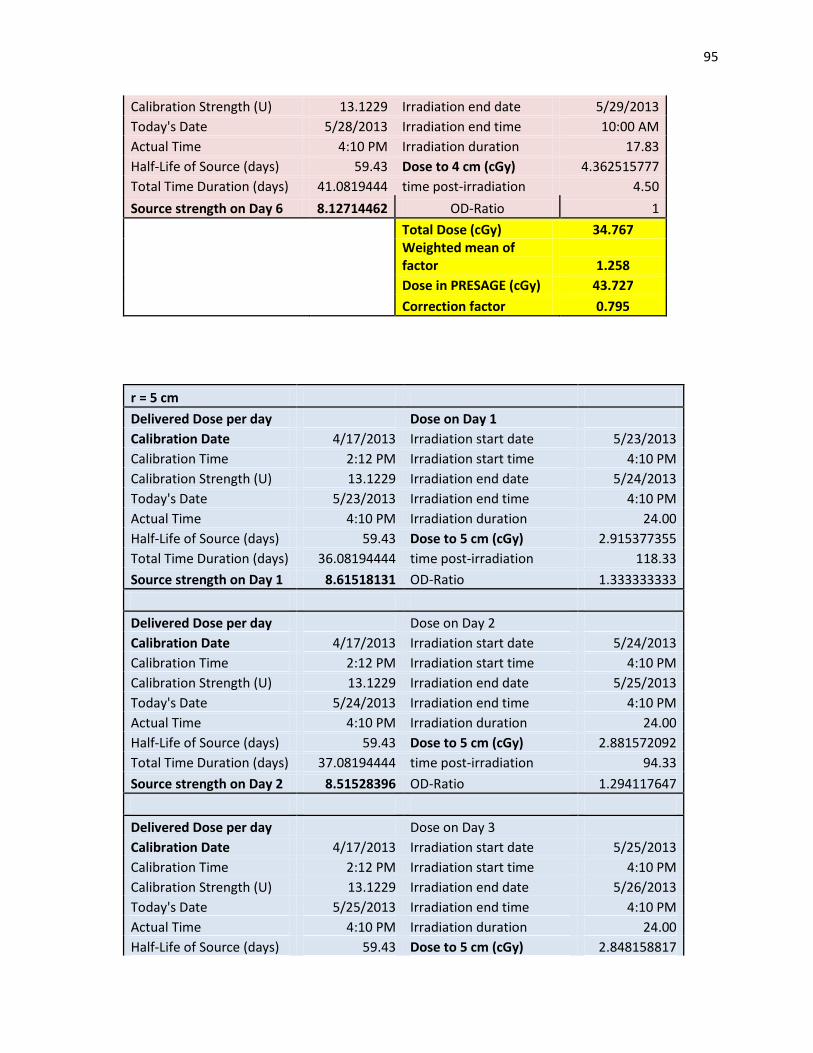
95
Calibration Strength (U) 13.1229 Irradiation end date 5/29/2013
Today's Date 5/28/2013 Irradiation end time 10:00 AM
Actual Time 4:10 PM Irradiation duration 17.83
Half-Life of Source (days) 59.43 Dose to 4 cm (cGy) 4.362515777
Total Time Duration (days) 41.0819444 time post-irradiation 4.50
Source strength on Day 6 8.12714462 OD-Ratio 1
Total Dose (cGy) 34.767
Weighted mean of factor 1.258
Dose in PRESAGE (cGy) 43.727
Correction factor 0.795
r = 5 cm
Delivered Dose per day Dose on Day 1
Calibration Date 4/17/2013 Irradiation start date 5/23/2013
Calibration Time 2:12 PM Irradiation start time 4:10 PM
Calibration Strength (U) 13.1229 Irradiation end date 5/24/2013
Today's Date 5/23/2013 Irradiation end time 4:10 PM
Actual Time 4:10 PM Irradiation duration 24.00
Half-Life of Source (days) 59.43 Dose to 5 cm (cGy) 2.915377355
Total Time Duration (days) 36.08194444 time post-irradiation 118.33
Source strength on Day 1 8.61518131 OD-Ratio 1.333333333
Delivered Dose per day Dose on Day 2
Calibration Date 4/17/2013 Irradiation start date 5/24/2013
Calibration Time 2:12 PM Irradiation start time 4:10 PM
Calibration Strength (U) 13.1229 Irradiation end date 5/25/2013
Today's Date 5/24/2013 Irradiation end time 4:10 PM
Actual Time 4:10 PM Irradiation duration 24.00
Half-Life of Source (days) 59.43 Dose to 5 cm (cGy) 2.881572092
Total Time Duration (days) 37.08194444 time post-irradiation 94.33
Source strength on Day 2 8.51528396 OD-Ratio 1.294117647
Delivered Dose per day Dose on Day 3
Calibration Date 4/17/2013 Irradiation start date 5/25/2013
Calibration Time 2:12 PM Irradiation start time 4:10 PM
Calibration Strength (U) 13.1229 Irradiation end date 5/26/2013
Today's Date 5/25/2013 Irradiation end time 4:10 PM
Actual Time 4:10 PM Irradiation duration 24.00
Half-Life of Source (days) 59.43 Dose to 5 cm (cGy) 2.848158817
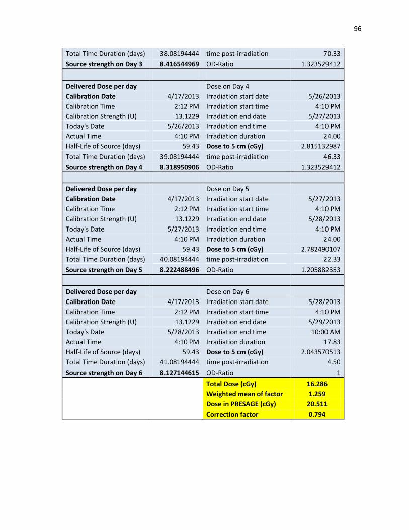
96
Total Time Duration (days) 38.08194444 time post-irradiation 70.33
Source strength on Day 3 8.416544969 OD-Ratio 1.323529412
Delivered Dose per day Dose on Day 4
Calibration Date 4/17/2013 Irradiation start date 5/26/2013
Calibration Time 2:12 PM Irradiation start time 4:10 PM
Calibration Strength (U) 13.1229 Irradiation end date 5/27/2013
Today's Date 5/26/2013 Irradiation end time 4:10 PM
Actual Time 4:10 PM Irradiation duration 24.00
Half-Life of Source (days) 59.43 Dose to 5 cm (cGy) 2.815132987
Total Time Duration (days) 39.08194444 time post-irradiation 46.33
Source strength on Day 4 8.318950906 OD-Ratio 1.323529412
Delivered Dose per day Dose on Day 5
Calibration Date 4/17/2013 Irradiation start date 5/27/2013
Calibration Time 2:12 PM Irradiation start time 4:10 PM
Calibration Strength (U) 13.1229 Irradiation end date 5/28/2013
Today's Date 5/27/2013 Irradiation end time 4:10 PM
Actual Time 4:10 PM Irradiation duration 24.00
Half-Life of Source (days) 59.43 Dose to 5 cm (cGy) 2.782490107
Total Time Duration (days) 40.08194444 time post-irradiation 22.33
Source strength on Day 5 8.222488496 OD-Ratio 1.205882353
Delivered Dose per day Dose on Day 6
Calibration Date 4/17/2013 Irradiation start date 5/28/2013
Calibration Time 2:12 PM Irradiation start time 4:10 PM
Calibration Strength (U) 13.1229 Irradiation end date 5/29/2013
Today's Date 5/28/2013 Irradiation end time 10:00 AM
Actual Time 4:10 PM Irradiation duration 17.83
Half-Life of Source (days) 59.43 Dose to 5 cm (cGy) 2.043570513
Total Time Duration (days) 41.08194444 time post-irradiation 4.50
Source strength on Day 6 8.127144615 OD-Ratio 1
Total Dose (cGy) 16.286
Weighted mean of factor 1.259
Dose in PRESAGE (cGy) 20.511
Correction factor 0.794

97
References
[1] J.M. F. Mourtada, G. Ibbott, Monte Carlo calculations of AAPM Task Group Report No.
43 dosimetry parameters for the I-125 I-seed AgX100 source model, Brachytherapy
11 (2012) 237-244.
[2] P.B. Z. Chen, R. Nath, Experimental Characterization of the Dosimetric Properties of a
newly designed I-Seed model AgX100 I-125 interstitial brachytherapy source,
Brachytherapy 11 (2012) 476-482.
[3] S. Webb, The physical basis of IMRT and inverse planning, The British Journal of
Radiology 76 (2003) 678-689.
[4] J.A. M. Oldham and H. Sakhalkar and P. Guo, An investigation of the accuracy of an
IMRT dose distribution using two- and three-dimensional dosimetry techniques,
Medical Physics 35 (2008) 2072-2080.
[5] e.a. L. M. Jampol, The COMS randomized trial of iodine 125 brachytherapy for
choroidal melanoma, Ophthalmology 109 (2002) 2197-2206.
[6] e.a. C. M. Yashar, Initial Clinical Experience with the Strut-Adjusted Volume Implant
(SAVI) Breast Brachytherapy Device for APBI: FIrst 100 Patients with more than 1
year of follow-up, International Journal of Radiation Oncology 80 (2011) 765-770.
[7] W.F.H. A. K. Krintz, G. S. Ibbott, D. S. Followill, A reanalysis of the Collaborative
Ocular Melanoma Study Medium Tumor Trial eye plaque dosimetry, International
Journal of Radiation Oncology 56 (2003) 889-896.
[8] K.L.L. N. L. Gagne, M. J. Rivard, Radiobiology for eye plaque brachytherapy and
evaluation of implant duration and radionuclide choice using an objective function,
Medical Physics 39 (2012) 3332-3342.
98
[9] P.M. Devlin, Brachytherapy Applications and Techniques, Lippincott Williams &
Wilkins, Philadelphia, 2007, pp. 1-5.
[10] L.S. D. Bates, N. Zamboglou, Medical Physics and Biomedical Engineering, Taylor &
Francis Group, LLC, Boca Raton, 2007.
[11] J.F. Williamson, Brachytherapy technology and physics practice since 1950: a half-
century of progress, Physics in Medicine and Biology 51 (2006) R303-R325.
[12] J.A.L. S. W. Chen, S. N. Yang, H.L Ko, F. J. Lin, The adverse effect of treatment
prolongation in cervical cancer by high dose rate intracavitary brachytherapy,
Radiotherapy and Oncology 67 (2003) 69-76.
[13] I. 38, Dose and volume specifications for reporting intracavitary therapy in gynecology,
International Commission on Radiation Units and Measurements, Bethesda, MD,
1985, pp. 1-23.
[14] B.M.C. M. J. Rivard, L.A. DeWerd, et al., Update of AAPM Task Group No. 43
Report: A revised AAPM protocol for brachytherapy dose calculations, Med Phys 31
(2004) 633-674.
[15] G.S.I. L. A. DeWerd, A. S. Meigooni, M. G. Mitch, M. J. Rivard, K. E. Stump, B. R.
Thomadsen, J. L. M. Venselaar, A dosimetric uncertainty analysis for photon-
emitting brachytherapy sources: Report of AAPM Task Group No. 138 and GEC-
ESTRO, Medical Physics 38 (2011) 782-801.
[16] J.A.P. S.H. Levitt, C.A. Perez, S. vijayakumar, Technial Basis of Radiation Therapy,
Springer-Verlag Berlin Heidelberg, 2006.
[17] I.J.S. C. C. Ling, J. Mitchell, R. Stickler, The Variation of OER with Dose Rate,
International Journal of Radiation Oncology 11 (1985) 1367-1373.
99
[18] P.M. Devlin, Brachytherapy Applications and Techniques, Lippincott Williams &
Wilkins, Philadelphia, 2007, pp. 52.
[19] S. Nag, High Dose Rate Brachytherapy: a textbook, Futura, New York.
[20] I. Medi-Physics, OncoSeed Iodine-125 Seeds, in: O.b.G. Healthcare (Ed.), 2009.
[21] R.E.M. H.L. Andrews, E. J. LeBrun, Gel Dosimeter for Depth-Dose Measurements,
Review of Scientific Instruments 28 (1957) 329-332.
[22] Y.S.K. J. C. Gore, R. J. Schulz, Measurement of radiation dose distributions by nuclear
magnetic resonance (NMR) imaging, Physics in Medicine and Biology 29 (1984)
1189-1197.
[23] B.A.W. L. E. Olsson, A. Fransson, B. Nordell, Diffusion of ferric ions in agarose
dosimeter gels Physics in Medicine and Biology 37 (1992) 2243-2252.
[24] P.J.H. C. Baldock, A. R. Piercy, B. Healy, Experimental determination of the diffucion
coefficient in two-dimensions in ferrous sulphate gels using the finite element
method., Australasian Physical & Engineering Sciences in Medicine 24 (2001) 19-
30.
[25] J.C.G. M. J. Maryanski, R. P. Kennan, R. J. Shulz, NMR Relaxation Enhancement in
gels polymerized and cross-linked by ionizing radiation: a new approach to 3D
dosimetry by MRI
Magnetic Resonance Imaging 11 (1993) 253-258.
[26] Y.D.D. C Baldock, S. Doran, G. Ibbott, A. Jirasek, M. Lepage, K. B. McAuley, M.
Oldham, L. J. Schreiner, Polymer Gel Dosimetry, Physics in Medicine and Biology
55 (2010) R1-R63.
100
[27] R.J.S. M. J. Maryanski, G. S. Ibbott, J. C. Gatenbym J. Xie, D. Horton, J. C. Gore,
Magnetic Resonance Imaging of Radiation Dose Distribution using a polymer-gel
dosimeter, Physics in Medicine and Biology 39 (1994) 1437-1455.
[28] M.R. J. C. Gore, M. J. Maryanski, R. J. Schulz, Radiation dose distributions in three
dimensions from tomographic optical density scanning of polymer gels: I.
Development of an optical scanner, Physics in Medicine and Biology 41 (1996)
2695-2704.
[29] Y.Z.Z. M. J. Maryanski, J. C. Gore, Radiation dose distributions in three dimensions
from tomographic optical density scanning of polymer gels: II. Optical properties of
the BANG polymer gel, Physics in Medicine and Biology 41 (1996) 2705-2717.
[30] J.H.S. M. Oldham, S. Kumar, J. Wong, D. A. Jaffray, Optical-CT gel-dosimetry I:
Basic investigations, Medical Physics 30 (2003) 623-635.
[31] L.K. M. Oldham, Optical-CT gel-dosimetry II: Optical artifacts and geometrical
distortion, Medical Physics 31 (2004) 1093-1205.
[32] J.A. P. Guo, M. Oldham, A practical three-dimensional dosimetry system for radiation
therapy, Med Phys 33 (2006) 3962-3972.
[33] M.J.M. J. Adamovics, New 3D radiochromic solid polymer dosimeter from leuco dyes
and a transparent polymeric matrix, Medical Physics 30 (2003) 1349-1349.
[34] M.J.M. J. Adamovics, Characterisation of PresageTM
: A New 3-D Radiochromic Solid
Polymer Dosemeter for Ionising Radiation, Radiation Protection Dosimetry 120
(2006) 107-112.
[35] J.A.A. P.Y. Guo, M. Oldham, Characterization of a new radiochromic three-
dimensional dosimeter, Med Phys 33 (2006) 1338-1345.

101
[36] J.A. H.S. Sakhalkar, G. Ibbott, M. Oldham, A comprehensive evaluation of the
PRESAGE/optical-CT 3D dosimetry system, Medical Physics 36 (2008) 71-82.
[37] M.O. A. Thomas, Fast, large field-of-view, telecentric optical-CT scanning system for
3D radiochromic dosimetry, Journal of Physics: Conference Series 250 (2010).
[38] J.A. A. Thomas and J. Newton, M. Oldham, Commissioning and benchmarking a 3D
dosimetry system for clincial use, Med Phys 38 (2011) 4846-4857.
[39] K.J. J. Adamovics, J. Dietrich, PRESAGE- Development and optimization studies of a
3D radiochromic plastic dosimeter- Part 1, Journal of Physics: Conference Series 56
(2006) 172-175.
[40] J.A. H. Sakhalkar and D. Sterling, G. Ibbott, M. Oldham, Investigation of the feasibility
of relative 3D dosimetry inthe Radiologic Physics Center Head and Neck IMRT
phantom using Presage/optical-CT, Medical Physics 36 (2009) 3371-3377.
[41] A.T. C. Clift, J. Adamovics, Z. Chang, I. Das, M. Oldham, Toward Acquiring
Comprehensive Radiosurgery Field Commissioning Data using the
PRESAGE/optical-CT 3D Dosimetry System, Institute of Physics and Engineering
in Medicine 55 (2010) 1279-1293.
[42] J.A. M. Heard, G. S. Ibbott, Measurement of a 200 MeV proton beam using a
polyurethane dosimeter, Journal of Physics: Conference Series 56 (2006).
[43] S.D. S. Al-Nowais, A. Kacperek, N. Krstajic, J. Adamovics, D. Bradley, A preliminary
analysis of LET effects in the dosimetry of proton beams using PRESAGE and
optical CT, Applied Radiation and Isotopes 67 (2009) 415-418.
102
[44] J.A. P. Wai, N. Krstajic, A. Ismail, A. Nisbet, S. Doran, Dosimetry of the
microSelectron-HDR Ir-192 source using PRESAGE and optical CT, Applied
Radiation and Isotopes 67 (2009) 419-422.
[45] R.H. T. Gorjiara, J. K. Kim, Z. Kuncic, J. Adamovics, C. Baldock, Study of dosimetric
water equivalency of PRESAGE for megavoltage and kilovoltage x-ray beams,
Journal of Physics: Conference Series 250 012053 (2010).
[46] A.I.B. J. O. Deasy, V. H. Clark, CERR: A computational environment for radiotherapy
research, Medical Physics 30 (2003) 979-987.
[47] F.M. Khan, The Physics of Radiation Therapy, 4 ed., Lippincott Williams & Wilkins,
Baltimore, 2010.

103
Olivia Huang was born in Columbia, Missouri on December 4, 1987 to the parents of Wei-an and
Meng-fen Huang. After completing her Human Biology Degree at the University of California, San
Diego in 2010, she entered the Medical Physics program at the University of Texas-Houston M.D.
Anderson Cancer Center. She completed her research project and the Specialized Masters Degree in
Medical Physics in August 2013.
Permanent Address:
20488 Chalet Lane
Saratoga, CA 95070
Email: