Evaluation of the Clearview Font for Negative Contrast … · EVALUATION OF THE CLEARVIEW FONT FOR NEGATIVE CONTRAST TRAFFIC SIGNS 6. Performing Organization Code 7. ... longer legibility

Technical Report Documentation Page 1. Report No. FHWA/TX-06/0-4984-1

2. Government Accession No.

3. Recipient's Catalog No. 5. Report Date January 2006 Resubmitted: April 2006

4. Title and Subtitle EVALUATION OF THE CLEARVIEW FONT FOR NEGATIVE CONTRAST TRAFFIC SIGNS

6. Performing Organization Code

7. Author(s) Andrew J. Holick, Susan T. Chrysler, Eun Sug Park, and Paul J. Carlson

8. Performing Organization Report No. Report 0-4984-1 10. Work Unit No. (TRAIS)

9. Performing Organization Name and Address Texas Transportation Institute The Texas A&M University System College Station, Texas 77843-3135

11. Contract or Grant No. Project 0-4984 13. Type of Report and Period Covered Technical Report: September 2004–November 2005

12. Sponsoring Agency Name and Address Texas Department of Transportation Research and Technology Implementation Office P.O. Box 5080 Austin, Texas 78763-5080

14. Sponsoring Agency Code

15. Supplementary Notes Project performed in cooperation with the Texas Department of Transportation and the U.S. Department of Transportation, Federal Highway Administration. Project Title: Evaluation of Clearview Font on Negative Contrast Signs URL: http://tti.tamu.edu/documents/0-4984-1.pdf 16. Abstract Texas Department of Transportation (TxDOT) sponsored research has shown that the Clearview font provides longer legibility distances than the Highway Gothic font Series E (Modified) when used on freeway guide signs with positive contrast of white letters on a dark background. Additional studies have shown that Clearview outperforms other versions of Highway Gothic fonts on other, smaller types of guide signs. These results have helped support the adoption of the Clearview font into the Federal Highway Administration’s (FHWA) Standard Highway Signs book. The Clearview font has been developed with two sets of fonts—one for positive contrast signs and another for negative contrast signs. Prior to this research project, there were no studies documenting the performance of the Clearview font for negative contrast signs such as those found in the regulatory and warning sign series. This research project evaluated the negative contrast Clearview font in black letters on fluorescent yellow, fluorescent orange, and white backgrounds. The researchers performed a laptop-based presentation survey and a closed-course field study. The laptop survey used static, in-context sign images to compare sign fonts. The field study was a dynamic recognition and legibility test using full-sized retroreflective signs during the day and at night. The field study compared the standard font to three treatments of the Clearview font. The results of this research project show that the Clearview font provides the same performance as the current FHWA font series for negative contrast traffic signs with the exception of the nighttime recognition. In this instance, the straight replacement of Clearview did not achieve similar recognition distances as the FHWA font series until the stroke width was increased to the next weight. The recognition distance provided by traffic signs can be considered one of the most critical measures of effectiveness when assessing sign performance. Therefore, because there were no statistically significant increases in recognition or legibility distances for any of the Clearview fonts tested, and because the results of the nighttime recognition analysis showed a decrease in recognition distance when the FHWA font was replaced with the Clearview font, the researchers recommend that TxDOT continue using the FHWA font series for negative contrast signs. 17. Key Words Clearview, Legibility, Recognition, Visibility, Negative Contrast, Older Driver, Highway Sign Font

18. Distribution Statement No restrictions. This document is available to the public through NTIS: National Technical Information Service Springfield, Virginia 22161 http://www.ntis.gov

19. Security Classif.(of this report) Unclassified

20. Security Classif.(of this page) Unclassified

21. No. of Pages 130

22. Price

Form DOT F 1700.7 (8-72) Reproduction of completed page authorized

http://tti.tamu.edu/documents/0-4984-1.pdf

http://www.ntis.gov

EVALUATION OF THE CLEARVIEW FONT FOR NEGATIVE CONTRAST TRAFFIC SIGNS

by

Andrew J. Holick Assistant Transportation Researcher

Texas Transportation Institute

Susan T. Chrysler, Ph.D. Research Scientist


Eun Sug Park, Ph.D. Assistant Research Scientist


and

Paul J. Carlson, Ph.D., P.E. Associate Research Engineer

Division Head Texas Transportation Institute

Report 0-4984-1 Project 0-4984

Project Title: Evaluation of Clearview Font on Negative Contrast Signs

Performed in cooperation with the Texas Department of Transportation

and the Federal Highway Administration

January 2006 Resubmitted: April 2006

TEXAS TRANSPORTATION INSTITUTE The Texas A&M University System College Station, Texas 77843-3135

v

DISCLAIMER

The contents of this report reflect the views of the authors, who are responsible for the

facts and the accuracy of the data presented herein. The contents do not necessarily reflect the

official view or policies of the Federal Highway Administration (FHWA) or the Texas

Department of Transportation (TxDOT). This report does not constitute a standard,

specification, or regulation. The United States Government and the State of Texas do not

endorse products or manufacturers. Trade or manufacturers’ names appear herein solely because

they are considered essential to the object of this report. The researcher in charge was Paul J.

Carlson, Ph.D., P.E. (TX, #85402).

vi

ACKNOWLEDGMENTS

This project was conducted in cooperation with TxDOT and FHWA. The researchers

would like to thank the project coordinator, Lauren Gardũno of the TxDOT Odessa District, for

providing guidance and expertise on this project. The authors would also like to thank the

members of the TxDOT project monitoring committee for their assistance:

• Brian Stanford, project director;

• Greg Brinkmeyer;

• Michael Chacon;

• Charlie Wicker; and

• Wade Odell.

The researchers would also like to thank several Texas Transportation Institute (TTI)

personnel for their invaluable help in completing this project:

• Dick Zimmer,

• Alicia Williams,

• Amanda Anderle Fling,

• Sara Meischen,

• Chris Rountree,

• Todd Hausman, and

• Dan Walker.

Finally, the authors would like to thank Don Meeker for his time and assistance.

Mr. Meeker visited with the project team to identify critical experimental factors and develop an

experimental plan for the research activities.

vii

TABLE OF CONTENTS

Page List of Figures............................................................................................................................. viii List of Tables ..................................................................................................................................x Chapter 1: Background and Significance of Work ...................................................................1

Clearview Background.................................................................................................................1 Research Findings........................................................................................................................2

Chapter 2: Experimental Procedure...........................................................................................7 Fonts and Sign Design .................................................................................................................7

Existing Sign Analysis.............................................................................................................7 Experimental Signs ................................................................................................................12

Materials ....................................................................................................................................13 Field Study Method....................................................................................................................13

Participants.............................................................................................................................13 Experimental Vehicle.............................................................................................................14 Experimental Design..............................................................................................................15 Experimental Procedure.........................................................................................................21

Laptop Study Method ................................................................................................................24 Participants.............................................................................................................................25 Data Collection ......................................................................................................................25

Chapter 3: Experiment Results .................................................................................................29 Laptop Study..............................................................................................................................29 Field Study.................................................................................................................................30

Recognition Task ...................................................................................................................31 Legibility Task .......................................................................................................................32

Field Study Statistical Analysis .................................................................................................35 Recognition Task ...................................................................................................................35 Legibility Task .......................................................................................................................41

Chapter 4: Conclusions ..............................................................................................................47 Discussion..................................................................................................................................47

Laptop Study..........................................................................................................................47 Field Study.............................................................................................................................47

Conclusions................................................................................................................................48 Recommendations......................................................................................................................49 Future Research .........................................................................................................................50

References.....................................................................................................................................51 Appendix A...................................................................................................................................53 Appendix B ...................................................................................................................................57 Appendix C...................................................................................................................................71 Appendix D...................................................................................................................................79 Appendix E ...................................................................................................................................87

viii

LIST OF FIGURES Page Figure 1. Clearview Positive and Negative Contrast Fonts. .......................................................... 2 Figure 2. Perpendicular Test Points. ............................................................................................. 8 Figure 3. Example of Sign Legend Modifications......................................................................... 9 Figure 4. 2001 Ford Taurus Test Vehicle. ................................................................................... 15 Figure 5. Nu-Metrics Nitestar DMI. ............................................................................................ 15 Figure 6. Driving Course and Sign Positions. ............................................................................. 21 Figure 7. “Starting Gate” Cones. ................................................................................................. 22 Figure 8. Recognition Task Course and Sign. ............................................................................. 23 Figure 9. Legibility Task Course and Signs in Daytime.............................................................. 24 Figure 10. Legibility Task Course and Signs at Night................................................................. 24 Figure 11. Laptop Presentation Image Showing Uppercase Font................................................ 26 Figure 12. Laptop Presentation Image Showing Mixed Case Font. ............................................ 27 Figure 13. Version B Answer Sheet Example for Laptop Study................................................. 27 Figure 14. Laptop Evaluation Version A Average Lines Correct. .............................................. 29 Figure 15. Laptop Evaluation Version B Percent Correct Response........................................... 30 Figure 16. Median Recognition Distance. ................................................................................... 31 Figure 17. Median Positive Recognition Distance. ..................................................................... 32 Figure 18. Younger Driver Mean Legibility Distance by Treatment. ......................................... 33 Figure 19. Older Driver Mean Legibility Distance by Treatment. .............................................. 33 Figure 20. Younger Driver Mean Legibility Distance by Treatment and Color. ........................ 34 Figure 21. Older Driver Mean Legibility Distance by Treatment and Color. ............................. 34 Figure 22. Interaction Plot of Day_Night*Treatment.................................................................. 37 Figure 23. Interaction Plot of Font Treatment*TargetLine. ........................................................ 37 Figure 24. Interaction Plot of Day_Night*Treatment.................................................................. 40 Figure 25. Interaction Plot of Treatment*TargetLine.................................................................. 40 Figure 26. Interaction Plot of Day_Night*Treatment.................................................................. 43 Figure 27. Interaction Plot of Treatment*NumLine. ................................................................... 43 Figure 28. Interaction Plot of Treatment*Color. ......................................................................... 44 Figure E-1. Interaction Plot for Day_Night*Treatment............................................................... 92 Figure E-2. Interaction Plot for Treatment*TargetLine............................................................... 93 Figure E-3. Interaction Plot for Day_Night*Treatment............................................................... 96 Figure E-4. Interaction Plot for Treatment*TargetLine............................................................... 97 Figure E-5. Interaction Plot for Day_Night*Treatment............................................................... 99 Figure E-6. Interaction Plot for Treatment*TargetLine............................................................. 100 Figure E-7. Interaction Plot for Treatment*TargetLine............................................................. 102 Figure E-8. Interaction Plot for Day_Night*Treatment without Outliers.................................. 105 Figure E-9. Interaction Plot for Treatment*TargetLine without Outliers.................................. 106 Figure E-10. Interaction Plot for Day_Night*Treatment without Outliers................................ 108 Figure E-11. Interaction Plot for Treatment*TargetLine without Outliers................................ 109 Figure E-12. Interaction Plot for Day_Night*Treatment........................................................... 112 Figure E-13. Interaction Plot for Treatment*Color. .................................................................. 113 Figure E-14. Interaction Plot for Treatment*NumLine. ............................................................ 114

ix

Figure E-15. Least Squares Means Plot for Conflict. ................................................................ 117 Figure E-16. Gender................................................................................................................... 118 Figure E-17. Age Group. ........................................................................................................... 118 Figure E-18. Visual Acuity. ....................................................................................................... 118 Figure E-19. Contrast Sensitivity............................................................................................... 118

x

LIST OF TABLES Page Table 1. Mean Legibility Distances for Positive and Negative Contrast Signs............................. 3 Table 2. Mean Legibility Distance by Sign Type. ......................................................................... 4 Table 3. Highway to Clearview Font Conversions...................................................................... 10 Table 4. Signs Used for Recognition Portion. ............................................................................. 17 Table 5. Signs Used for Legibility Portion for Yellow Warning Signs....................................... 18 Table 6. Signs Used for Legibility Portion for Orange Warning Signs....................................... 19 Table 7. Signs Used for Legibility Portion for White Regulatory Signs. .................................... 20 Table 8. Signs Used in Laptop Presentation. ............................................................................... 26 Table 9. Recognition Distance Analysis Summary of Fit............................................................ 35 Table 10. Recognition Distance Analysis Effects Test................................................................ 36 Table 11. Tukey’s Multiple Comparison Test for Day_Night*Treatment. ................................. 38 Table 12. Tukey’s Multiple Comparison Test for Treatment*TargetLine. ................................. 38 Table 13. Postive Recognition Distance Analysis Summary of Fit............................................. 39 Table 14. Postive Recognition Distance Analysis Effects Test. .................................................. 39 Table 15. Tukey’s Multiple Comparison Test for Day_Night*Treatment. ................................. 41 Table 16. Tukey’s Multiple Comparison Test for Treatment*TargetLine. ................................. 41 Table 17. Legibility Analysis Summary of Fit. ........................................................................... 42 Table 18. Legibility Analysis Effects Test. ................................................................................. 42 Table 19. Tukey’s Multiple Comparison Test for Day_Night*Treatment. ................................. 44 Table 20. Tukey’s Multiple Comparison Test for Treatment*NumLine..................................... 45 Table 21. Tukey’s Multiple Comparison Test for Treatment*Color. .......................................... 45 Table A-1. Laptop Evaluation Sign Images.................................................................................. 55 Table C-1. Recognition Data Case Summary, Day. ..................................................................... 73 Table C-2. Recognition Data Case Summary, Night. ................................................................... 74 Table C-3. Positive Recognition Data Case Summary, Day. ....................................................... 75 Table C-4. Positive Recognition Data Case Summary, Night. ..................................................... 76 Table C-5. Recognition Case Summary, Collapsed Categories. .................................................. 77 Table C-6. Positive Recognition Case Summary, Collapsed Categories...................................... 78 Table D-1. Legibility Case Summary, Younger Driver, Day. ...................................................... 81 Table D-2. Legibility Case Summary, Older Driver, Day............................................................ 82 Table D-3. Legibility Case Summary, Younger Driver, Night..................................................... 83 Table D-4. Legibility Case Summary, Older Driver, Night. ........................................................ 84 Table D-5. Legibility Data Case Summary, Collapsed Categories. ............................................. 85 Table E-1. Categorization of Variables Visual Acuity and Contrast Sensitivity.......................... 90 Table E-2. JMP Output for Rec_Dist under Model A. ................................................................. 91 Table E-3. Tukey’s Multiple Comparison Test for Day_Night*Treatment. ................................ 92 Table E-4. Tukey’s Multiple Comparison Test for Treatment*TargetLine. ................................ 93 Table E-5. JMP Output for Rec_Dist under Model B. ................................................................. 95 Table E-6. Tukey’s Multiple Comparison Test for Day_Night*Treatment. ................................ 96 Table E-7. Tukey’s Multiple Comparison Test for Treatment*TargetLine. ................................ 97 Table E-8. JMP Output for Pos_Rec under Model A. .................................................................. 98 Table E-9. Tukey’s Multiple Comparison Test for Day_Night*Treatment. ................................ 99

xi

Table E-10. Tukey’s Multiple Comparison Test for Treatment*TargetLine. ............................ 100 Table E-11. JMP Output for Rec_Dist under Model B. ............................................................. 101 Table E-12. Tukey’s Multiple Comparison Test for Treatment*TargetLine. ............................ 102 Table E-13. JMP Output for Pos_Rec under Model A without Five Outliers. ........................... 104 Table E-14. Tukey’s Multiple Comparison Test for Day_Night*Treatment without

Outliers................................................................................................................................ 105 Table E-15. Tukey’s Multiple Comparison Test for Treatment*TargetLine without

Outliers................................................................................................................................ 106 Table E-16. JMP Output for Rec_Dist under Model B without Outliers. .................................. 107 Table E-17. Tukey’s Multiple Comparison Test for Day_Night*Treatment. ............................ 108 Table E-18. Tukey’s Multiple Comparison Test for Treatment*TargetLine without

Outliers................................................................................................................................ 109 Table E-19. JMP Output for Leg_Dist........................................................................................ 111 Table E-20. Tukey’s Multiple Comparison Test for Day_Night*Treatment ............................. 112 Table E-21. Tukey’s Multiple Comparison Test for Treatment*Color ...................................... 113 Table E-22. Tukey’s Multiple Comparison Test for Treatment*NumLine................................ 114 Table E-23. JMP Output for Adjusted Leg_Dist. ....................................................................... 116 Table E-24. Least Squares Means Table for Conflict................................................................. 117

1

CHAPTER 1: BACKGROUND AND SIGNIFICANCE OF WORK

CLEARVIEW BACKGROUND

The ClearviewHwy™ font, hereafter referred to as Clearview, was developed for traffic

signs for the Federal Highway Administration (FHWA) by a design team that included Donald

Meeker and Christopher O’Hara of Meeker and Associates, Inc.; James Montalbano of Terminal

Design, Inc.; and Martin Pietrucha, Ph.D., and Philip Garvey of the Pennsylvania Transportation

Institute, with supporting research by Gene Hawkins, Ph.D., and Paul Carlson, Ph.D., and advice

on research design by Susan Chrysler, Ph.D., of the Texas Transportation Institute.

Clearview was developed for traffic signs as the result of a research program to increase

the legibility and ease of recognition of positive contrast sign legends while reducing the effects

of halation (or overglow) for older drivers and drivers with reduced contrast sensitivity when

letters are displayed with high-brightness retroreflective materials. Specifically, the research

program worked to identify ways to create a more effective typeface than E-Modified as used for

destination legends on freeway guide signs. A second component of the original project was to

compare the ease of recognition of mixed case displays in lieu of all uppercase letter displays

(Series D), and to learn if a mixed case display would need to be larger than the comparable all

uppercase letter display for improved legibility and ease of recognition. By allowing a viewer to

read the footprint of the word when displayed in upper- and lowercase letters, similar to printed

text; accuracy, viewing distance, and reaction time increase (1).

The new Clearview font is provided in five weights (see Figure 1). Each weight is

specified with two versions: one for use in positive contrast applications (light tone letter on a

dark background) and one for use in negative contrast applications (dark tone letter on a light

background). The negative contrast version is optically adjusted to appear the same weight as

the positive contrast version but has a slightly heavier stroke width than the positive contrast

version. Meeker and Associates developed the negative contrast version following the same

design principles used for the positive contrast version. The negative contrast version, however,

had not ever been subjected to legibility testing.

2

Figure 1. Clearview Positive and Negative Contrast Fonts.

It should be noted that Clearview was designed for optimal legibility on the interior of the

letterforms and has a much different visual structure than the Highway Gothic series. The two

primary differences are: the lowercase letters are taller and the interior shapes of the letters are

more open, and the letter spacing for the lowercase Clearview is much more open than the 2000

Highway Gothic to accommodate the needs of older drivers when viewed at the appropriate

distance. To that end, transitioning from the Highway Gothic series to Clearview is not a

seamless one-for-one conversion of font series.

RESEARCH FINDINGS

The Clearview font provides increased legibility for positive contrast overhead and

ground-mounted guide signs (1-4). Researchers at the Pennsylvania Transportation Institute

performed the first Clearview study (1). Since then, three studies have been completed at the

Texas Transportation Institute and sponsored by the Texas Department of Transportation

(TxDOT) (2-4). In fact, TxDOT has recently adopted new signing practices for guide signs,

using the Clearview 5WR font and microprismatic sheeting for legends on all overhead signs and

large ground-mounted guide signs and the Clearview 3W font with microprismatic legend for

destination/distance signs (5). All of the previous Clearview research focused on positive

contrast guide signs, specifically signs with a white legend on green background. These studies

3

have shown that the Clearview font for positive contrast signs was not as easy to implement as

originally thought. Therefore, there is a significant need to perform research with respect to the

Clearview font for negative contrast signs before it should be implemented on a widespread

basis.

Chrysler, Carlson, and Hawkins (6) reported on a study evaluating the nighttime legibility

of ground-mounted traffic signs. The study evaluated shoulder-mounted conventional road guide

signs, warning signs, and regulatory signs. In the negative contrast sign applications, the

researchers compared yellow, fluorescent orange, and white backgrounds with a black legend.

The legibility of Highway Series D was evaluated against a font called D-Modified. D-Modified

has a thicker stroke width over that of Highway Series D. A white legend on a green background

was evaluated for the positive contrast sign application, and Highway Series D was evaluated

against Clearview Road Condensed. In addition, each color combination was tested using

Type III, Type VIII, and Type IX sheetings. The comparison of positive contrast and negative

contrast sign legibility (Table 1) is important. The results indicate that color may have an

influence on sign legibility. The white negative contrast signs performed similarly to the green

positive contrast signs, while the yellow negative contrast signs performed better than the green

positive contrast signs. In addition, the negative contrast orange signs performed considerably

worse than any other sign color combination.

Table 1. Mean Legibility Distances for Positive and Negative Contrast Signs.

Font Sheeting Color Mean (ft) Std. Dev. (ft) Green 179 68 Orange 143 61 White 180 66 Highway Series D Type III

Yellow 186 74

This study evaluated Clearview for positive contrast signs only; however, the font is an

older version of the Clearview font. The researchers found that the particular version (in all

uppercase letters) did not provide an increase in legibility distance over that of Highway

Series D. Also, the researchers determined that the D-Modified font did not improve legibility of

the negative contrast traffic signs. The report recommended that no changes be made to the

existing font standards for all uppercase legends on negative contrast signs (black letters on

white, yellow, or orange backgrounds). The current study expands this research on negative

contrast signs to examine the effects of replacing all uppercase legends in Highway Gothic

4

Series D with mixed upper/lowercase legends in the Clearview font designed for negative

contrast applications.

Zwahlen and Schnell also investigated conventional traffic sign legibility using negative

contrast signs (6). In both daytime and nighttime conditions, Zwahlen and Schnell tested three

negative contrast signs and one positive contrast sign. The signs were:

• black legend on white background, DO NOT PASS;

• black legend on orange background, NO EDGE LINES;

• black legend on yellow background, PLANT ENTRANCE; and

• white legend on green background, RUN CREEK.

The researchers found that daytime legibility distances for all signs were consistently

higher than nighttime legibility distances. Table 2 lists the mean legibility distances by sign

type.

Table 2. Mean Legibility Distance by Sign Type.

Sign Legend Condition Mean Legibility Distance (ft) Std. Dev. (ft)

Day 412.3 93.5 DO NOT PASS Series C Night 232.9 53.1 Day 543.5 150.2 NO EDGE

LINES Series D Night 316.5 80.7 Day 411.6 93.8 PLANT

ENTRANCE Series C Night 220.7 76.4 Day 852.5 179.4 RUN CREEK Series E Night 557.3 137.8

Within the negative contrast signs, Zwahlen and Schnell’s results indicate that white and

yellow negative contrast signs perform similarly, which agrees with Chrysler, Carlson, and

Hawkins. Zwahlen and Schnell did not control legend size or font type. The dramatically

increased legibility distance of orange background signs can be attributed to the Series D font as

compared to Series C. Series D has a heavier stroke width, wider letter form, and greater inter-

letter spacing than Series C. Zwahlen and Schnell also found increased legibility distances for

the white on green Series E font sign, which has an even more expanded letter form and spacing.

In the same study, Zwahlen and Schnell performed a recognition study using Landholt

rings on positive and negative contrast signs. Comparing the text legibility results to the

Landholt ring results, the researchers found that the results were in close agreement during the

5

daytime condition; however, during the nighttime condition, the Landholt rings did not perform

as well as the text legend. The researchers attributed this partly to the thicker stroke width of the

Landholt rings as compared to the text legend.

The research projects summarized above show that negative contrast signs typically have

a shorter legibility distance than comparable positive contrast signs. In addition, they also

indicate that font and color may interact (stroke width, letter height, and/or spacing in

combination with yellow, white, or orange color) to affect legibility. The current study

examined several variations of the Clearview negative contrast font rendered in black letters on

white, yellow, and orange backgrounds.

7

CHAPTER 2: EXPERIMENTAL PROCEDURE

The researchers conducted a daytime and nighttime legibility and recognition experiment

to assess the performance of the Clearview font designed for negative contrast ground-mounted

signs. This chapter describes the experimental procedures, including the sign materials, sign

layout, and font selection. Prior to the design of the experiments, the research team performed

an analysis of existing negative contrast ground-mounted signs. In this initial analysis, the

researchers replaced the Standard Highway series font on existing signs with the corresponding

Clearview font using sign layout software. This allowed the researchers to identify sign design

elements affected by changing from Highway Gothic to Clearview font. Once the study signs

were designed, two methods were used to evaluate the Clearview font: a laptop-based

presentation where subjects were shown static images of signs and asked to read the legend, and

a field study where subjects drove a test vehicle over a closed road course reading test signs.

FONTS AND SIGN DESIGN

This project focused on ground-mounted right shoulder signs, such as regulatory,

warning, and construction work zone signs. The research team was also interested in

determining the consistency of existing sign design within the Standard Highway Signs Design

(SHSD) manual. A thorough review of the TxDOT Standards and Specifications Sheets and the

Texas Standard Highway reference material revealed a variety of fonts used on these signs.

Existing Sign Analysis

Using the Texas Manual on Uniform Traffic Control Devices (TMUTCD), the research

team, with advice from the Project Monitoring Committee, selected several yellow and orange

warning signs as well as several black on white regulatory signs to study initially. The signs

were chosen because of their lengthy words, multiple lines of text, and possibly interfering

ascenders and decenders (letters that fall above or below the baseline). A particular concern

arises for these classes of signs because they include diamond shapes. For certain long words

and multi-line messages, a word can impinge on the border of a diamond-shaped sign very

easily. When the legends are converted from all uppercase to mixed case, there is a risk that

descending letters (such as g, j, and p) could come so close to the border as to affect legibility.

8

Using sign layout software, the research team recreated the selected signs following the

TMUTCD specifications. Once the signs were created in the sign software, a “perpendicular

test” and other appropriate measurements were made. The perpendicular test involved

measuring the perpendicular distance from the sign’s border to the most outer edges of text (see

Figure 2). If the distance was less than the border width, then the test was considered to have

failed. The other measurements made were the sign size, word lengths, inter-line spacing, letter

height, and inter-letter spacing.

Figure 2. Perpendicular Test Points.

The research team developed a series of seven modifications that could be made to each

of the signs in an attempt to pass the perpendicular test. After each modification the

perpendicular test was applied and all of the appropriate measurements were recorded. The

modifications are listed below; Figure 3 compares all the changes made to one particular sign.

This systematic analysis of the possible modifications essentially examined what could

be done to a particular legend to make it best fit the sign blank after the font was changed from

the Highway Gothic series to the Clearview series. The modifications boil down to changes in

inter-letter spacing, letter height, letter series, or inter-line spacing.

Perpendicular Test Points

9

Figure 3. Example of Sign Legend Modifications.

Spacing

p-carlson

Stamp

10

Modification 1: Straight Clearview Replacement. The first change to be made was to do

a straight replacement of the existing Highway Gothic font with the appropriate Clearview font

seen in Table 3. This table was provided to FHWA by Meeker and Associates and is based on

stroke width and letter height:width correspondences between the Highway Gothic series and the

Clearview B series. The letter B stands for “black letter” and denotes the Clearview series

designed for use on negative contrast signs. After the font substitution was made, the legend was

changed from all uppercase words to upper/lowercase. In some cases, the font and case changes

resulted in the legend touching or exceeding the border. For these cases, which typically had

three-line messages and longer words, additional modifications were attempted to make the

legend fit the sign blank. In other cases with short words or two-line messages, the

modifications were made to make use of the additional space remaining on the sign blank.

Table 3. Highway to Clearview Font Conversions. Highway Font Clearview Font

Series B Clearview 1B Series C Clearview 2B Series D Clearview 3B Series E Clearview 4B Series E-Modified Clearview 5B Series F Clearview 6B

Modification 2: Clearview Replacement at 100 Percent Spacing. The TMUTCD

requirements for specific legends include many instances of condensed inter-letter spacing

(kerning) to make longer words fit on standard sign blank sizes. For these cases, the second

modification took the new Clearview sign and changed the legend spacing to 100 percent.

Modification 3: Change in Inter-letter Spacing. Beginning with the Straight Clearview

Replacement sign, the inter-letter spacing was altered manually per line of text to allow

approximately one border length clearance when conducting the perpendicular test. This

modification increased or decreased the inter-letter spacing for each individual word to fit the

sign blank.

Modification 4: Change in Letter Height. Again, beginning with the Straight Clearview

Replacement, the letter height was altered for the entire legend to allow approximately one

border length clearance when conducting the perpendicular test. For some legends, this change

11

was a reduction in letter height, and for others the letter height was increased to take advantage

of available space on the sign blank.

Modification 5: Change in Series. Beginning with the Straight Clearview Replacement,

the font type was changed to another Clearview “B” font so that the legend allowed

approximately one border length clearance when conducting the perpendicular test. The change

in series was dependent on the sign legend. Longer legends were typically reduced to a lower

number series which had a narrower stroke width and more condensed letter form, while shorter

legends were increased to a larger number series with a thicker stroke width.

Modification 6: Change in Inter-line Spacing. Beginning with the Straight Clearview

Replacement sign, the inter-line spacing was changed in ¼-inch increments to allow

approximately one border length clearance when conducting the perpendicular test.

Modification 7: Change in Letter Height plus Kerning Spacing. Finally, beginning with

the Modification 4 version where the letter height has been changed, the kerning spacing was

varied to allow approximately one border length clearance when conducting the perpendicular

test. This modification was tested to examine what adjustments in kerning could be made after

the letter height was changed.

TXDOT Input

The results of the initial analysis and modifications were presented to the research panel

in January 2005. The results of the research panel meeting helped define the focus for the data

collection phase of the project. Several of the modifications made in the paper analysis were

deemed unfruitful for implementation and were dropped from further consideration. In

particular, the recommendations from the panel meeting were:

• maintain letter height between fonts, i.e., a smaller height Clearview letter should not

be substituted for a larger height Highway Gothic letter;

• test a straight substitution of the Clearview font;

• increase spacing, both inter-line and inter-letter;

• increase Clearview font series;

• use 36-inch warning signs; and

• use one type of prismatic retroreflective sheeting.

12

The research panel also identified 12 signs considered to be used frequently on the

roadway. The research panel requested that these signs be evaluated by the research team.

These 12 signs were:

• Right Lane Ends,

• Highway Intersection Ahead,

• Narrow Bridge,

• Divided Highway Ends,

• Be Prepared to Stop,

• Road Work Ahead,

• Road Work Next 5 Miles,

• Left Lane Closed,

• Pass with Care,

• Do Not Cross Double White Lines,

• Slower Traffic Keep Right, and

• Left Lane for Passing Only.

Experimental Signs

Signs to be used in the legibility tests were developed using sign layout software. The

specific font on each sign tested depended mostly on message length, with more condensed fonts

used on longer messages. In addition to the font identification, the TMUTCD sign analysis

revealed that the most common letter height was 5 inches. Thus, all words used in the nighttime

legibility project were 5-inch letters for uppercase letters with the lowercase letters automatically

sized by the font software. All of the sign layouts were created by TTI staff using the sign layout

software. The resulting files were transmitted electronically to the fabricator.

The project compared four font treatments:

1. standard all uppercase alphabet (Highway Gothic Series C or D) and spacing;

2. Clearview upper/lowercase straight replacement using 2B for Series C and 3B for

Series D and whatever condensed spacing is standard (Modification 1 above);

3. increase in the series of Clearview—if a sign had Series C, use 3B instead of 2B

(Modification 5 above); and

13

4. adjustments to font treatment 2 at the research team’s discretion including adjusting

inter-line spacing and kerning (combination of Modifications 3 and 6 above).

Appendix B contains measured drawings of all the signs used in the study. The words

used were selected from a list of frequent, non-traffic words. Random words were selected to

reduce any effects of drivers recognizing commonly seen traffic signs. All words were six letters

long to minimize reading time due to word familiarity or length.

MATERIALS

Based on the research panel’s recommendation, one type of retroreflective sheeting was

used for all signs tested: ASTM Type IX, a high-intensity microprismatic material (minimum

new RA at 0.2o observation angle and –4 o entrance angle for white material of 380 cd/lx/m2 and

240 cd/lx/m2 at 0.5 o observation angle and –4 o entrance angle). The material was provided by

the 3M Company as Diamond Grade™ VIP™.

Three colors of signs were tested:

• fluorescent yellow,

• fluorescent orange, and

• white.

The warning and work zone signs were all 36-inch diamonds. The white regulatory signs

were 36 inches wide and 30 inches high. The signs were mounted on aluminum substrates and

oriented 90° to the testing approach. The signs were mounted at a height of 7 ft to the bottom of

the sign and offset approximately 18 ft from the driving lane.

FIELD STUDY METHOD

The research team created a driving course containing the test signs at the Riverside

Campus of Texas A&M University. A group of 34 participants between the ages of 20 and 71

drove the course both during the day and at night while attempting to read the signs. This

section describes the study method.

Participants

Thirty-four licensed drivers were recruited for the project through personal contacts and

past research participant lists. Ten participants were between the ages of 55 and 71, and twenty-

14

four were between 20 and 55 years old. Eighteen males and sixteen females participated.

Subjects were paid $60 for their participation in both the daytime and nighttime portions which

took place on separate days. When the subjects arrived, they were briefed on the purpose of the

project, but no details of the font manipulation were revealed. After reading and signing an

informed consent form, the subject’s vision was tested. Binocular acuity was assessed using a

standard Snellen eye chart under room illumination. Contrast sensitivity was measured using the

VisTech™ Vision contrast test system. This test asks subjects to identify the orientation of a

series of sine wave gratings that vary in their contrast. Color vision was tested by using a

simplified Ishihara color plate. Participants completed a short questionnaire about their driving

habits. Two participants with visual acuity worse than required for a Texas driver’s license

(20/40) were excluded from the study. One participant reported color blindness.

Experimental Vehicle

All nighttime testing took place after sunset using low-beam headlamps. All daytime testing took

place between 9:00 AM and 6:00 PM to avoid the sun being low in the sky. The test vehicle was

a 2001 Ford Taurus sedan with HB4 halogen headlamps (Figure 4) equipped with a Nu-Metrics

Nitestar distance measuring instrument (DMI) (Figure 5). The windshield and headlamps were

cleaned at the start of each night’s testing.

15

Figure 4. 2001 Ford Taurus Test Vehicle.

Figure 5. Nu-Metrics Nitestar DMI.

Experimental Design

For the field study, each word was randomly assigned to a font-color sign condition.

Each word occurred only once. Each unique sign (Signs 1-44) were randomly assigned a post

position on the course. Since the same participants viewed the signs day and night, a different

target word or target line was used for the day and night portions of the study. Table 4 shows the

words and font treatments used for the signs in the recognition portion. Table 5 through Table 7

show the details for the signs used in the legibility portion of the study. Sign layout information

is given in Appendix B. Care was taken to ensure that the pattern of ascending and descending

letters was controlled. One disadvantage of moving to a mixed case font is that descending

letters on the first line may interfere visually with ascending letters on the second line. The test

signs were purposely designed to maximize the occurrence of this potential interference to make

the legibility most challenging.

16

The research team had some initial concerns that the specific sign locations might affect

legibility distance. While the test course is generally very dark, a few outdoor lights and other

objects may have posed a slight distraction to the driver. In addition, some locations were

preceded by more complicated driving maneuvers that may also have distracted participants from

the legibility task. One would expect some learning to take place, so the initial sign positions

might be at a disadvantage as well. In order to minimize any systematic effects of sign position,

the placement of the signs along the course was randomly determined. This random placement

was accomplished by treating each sign position as an independent location and numbering the

locations sequentially according to the driving path. Then each sign was randomly assigned a

number and placed in that location. Due to the labor involved in rearranging the signs, it was not

feasible to change them after every subject or even after every night of testing. Instead, a

compromise was reached to create two sign orders and change the signs after every set of eight

subjects.

Because the test facility was limited in the number of sign positions, a limited number of

signs could be prepared. Ideally, each manipulation of the font would have occurred more than

once on both two- and three-line signs. For the yellow signs, the most prevalent sign in the

TMUTCD had a two-line message. So for yellow test signs, there were two instances of two

lines and one instance of three lines. The opposite was true for orange and white signs. This

resulted in a slightly unbalanced design which can be accommodated for in the final statistical

analysis.

17

Table 4. Signs Used for Recognition Portion. Recognition Signs

Sign Number 1 2 3 4 5 6 7 8 Color White White White White White White White White

Treatment A B C D A B C D 2/3 Line 3 3 3 3 3 3 3 3

Repetition 1 1 1 1 2 2 2 2 Code Y2A1 Y2B1 Y2C1 Y2D1 Y2A2 Y2B2 Y2C2 Y2D2 Line 1 COLONY Giving Hungry Couple JUNGLE Spread Forget Family Line 2 SUMMER Season Famous Reason CORNER Crease Common Course Line 3 INSIDE Chance School Strike BETTER Double Travel Finish

Ascender/None/Descender Pattern Line 1 D SD D D D D Line 2 N N N N N N Line 3 A A A A A A

Target Word Day COLONY Chance Famous Couple BETTER Crease Forget Finish

Night SUMMER Giving School Reason JUNGLE Double Common Family Target Line

Day Top Bottom Middle Top Bottom Middle Top Bottom Night Middle Top Bottom Middle Top Bottom Middle Top

Note: Words were randomly assigned to treatment condition.

18

Table 5. Signs Used for Legibility Portion for Yellow Warning Signs.

Legibility Signs Sign Number 9 10 11 12 13 14 15 16 17 18 19 20

Color Yellow Yellow Yellow Yellow Yellow Yellow Yellow Yellow Yellow Yellow Yellow Yellow Treatment A B C D A B C D A B C D 2/3 Line 2 2 2 2 2 2 2 2 3 3 3 3

Repetition 1 1 1 1 2 2 2 2 1 1 1 1 Code Y2A1 Y2B1 Y2C1 Y2D1 Y2A2 Y2B2 Y2C2 Y2D2 Y3A Y3B Y3C Y3D Line 1 PEOPLE Change Always Enough SIMPLE Object Happen Though LENGTH Thirty Appear Strong Line 2 LITTLE Differ Animal Silent DESIGN Spring Degree Engine ANSWER Arrive Person Govern Line 3 NUMBER Before Mother Father

Ascender/None/Descender Pattern Line 1 D D D D D D D D D D D D Line 2 A A A A D D D D N N N N Line 3 A A A A

Target Word Day PEOPLE Differ Always Silent SIMPLE Spring Happen Engine LENGTH Arrive Mother Father

Night LITTLE Change Animal Enough DESIGN Object Degree Though ANSWER Before Person Strong Target Line

Day Top Bottom Top Bottom Top Bottom Top Bottom Top Middle Bottom Bottom Night Bottom Top Bottom Top Bottom Top Bottom Top Middle Bottom Middle Top


18

19

Table 6. Signs Used for Legibility Portion for Orange Warning Signs.


Color Orange Orange Orange Orange Orange Orange Orange Orange Orange Orange Orange Orange Treatment A B C D A B C D A B C D 2/3 Line 2 2 2 2 2 2 2 2 3 3 3 3

Repetition 1 1 1 1 2 2 2 2 1 1 1 1 Code O2A1 O2B1 O2C1 O2D1 O2A2 O2B2 O2C2 O2D2 O3A O3B O3C O3D Line 1 DURING System Bigger Weight SQUARE Length Region Energy BRIGHT Finger Twenty Symbol Line 2 MOTION Nature Market Branch LARGER Rising Longer Supper ACROSS Screen Thrown Income Line 3 BEAUTY Ground Public Rubber

Ascender/None/Descender Pattern Line 1 D D D D D D D D D D D D Line 2 A A A A D D D D N N N N Line 3 A A A A

Target Word Day DURING Nature Bigger Branch SQUARE Rising Region Supper BRIGHT Screen Public Rubber

Night MOTION System Market Weight LARGER Length Longer Energy ACROSS Ground Thrown Symbol Target Line

Day Top Bottom Top Bottom Top Bottom Top Bottom Top Middle Bottom Bottom Night Bottom Top Bottom Top Bottom Top Bottom Top Middle Bottom Middle Top


19

20

Table 7. Signs Used for Legibility Portion for White Regulatory Signs.


Color White White White White White White White White White White White White Treatment A B C D A B C D A B C D 2/3 Line 2 2 2 2 3 3 3 3 3 3 3 3

Repetition 1 1 1 1 1 1 1 1 2 2 2 2 Code W2A W2B W2C W2D W3A1 W2B1 W3C1 W3D1 W3A2 W3B2 W3C2 W3C2 Line 1 EXPECT Caught Pretty Magnet DEPEND Danger Repeat Valley PROPER Speech Bought Liquid Line 2 FACTOR Yellow Golden Listen PLENTY Safety String Likely SCREEN Lesson Dinner Cheese Line 3 WINDOW Wooden Settle Muscle MINUTE Rabbit Worker Modern

Ascender/None/Descender Pattern Line 1 D D D D D D D D D D D D Line 2 A A A A B B B B N N N N Line 3 A A A A A A A A

Target Word Day EXPECT Yellow Pretty Listen DEPEND Safety Settle Muscle PROPER Lesson Worker Modern

Night FACTOR Caught Golden Magnet PLENTY Wooden String Valley SCREEN Rabbit Dinner Liquid Target Line

Day Top Bottom Top Bottom Top Middle Bottom Bottom Top Middle Bottom Bottom Night Bottom Top Bottom Top Middle Bottom Middle Top Middle Bottom Middle Top


20

21

Experimental Procedure

A test course with 44 sign positions was laid out on a closed-course facility (see Figure

6). All signs were offset 18 ft from the right edge line with a height of 7 ft to the bottom of the

sign. The driving path was clearly delineated by the use of retroreflective raised pavement

markers. The sign positions were 500 ft apart at a minimum.

Figure 6. Driving Course and Sign Positions.

The research participants performed two types of reading tasks while driving the test

vehicle. In the recognition task, the participant had to report on which line of the sign a target

word appeared. This task theoretically should benefit from the “footprint” afforded by a mixed

case alphabet. In the legibility task, the participant had to read the word on a specified line of the

sign. This task should be more controlled by letter height and visual acuity.

The experimenter was seated in the front passenger seat and recorded all responses on

paper (illuminated by a flashlight with a red filter at night). The researcher provided verbal

directions to the subject regarding where to drive and the maximum speed allowed on the course

segment. At the start of each straight segment of road, a pair of traffic cones marked the

“starting gate” (Figure 7), which served to notify the subject that a sign was coming soon, and it

414243 44

Riverside Campus Runways

22

also gave the experimenter a chance to clear the DMI. Errors in measurements can be introduced

following the hard corners and U-turns necessitated by the test course.

The driving course took approximately 35 minutes to complete. If participants made any

comments during the study, these were noted on the response form.

Figure 7. “Starting Gate” Cones.

Recognition Task

Participants drove the test vehicle at a slow speed, essentially coasting (between 5 to

10 mph) toward each test sign (Figure 8). At the start of each trial, and about halfway through,

the experimenter announced the target word to the participant who was to verbally respond

“top,” “middle,” or “bottom” to indicate the position of the target word. Participants were

encouraged, and at far distances forced, to guess. At approximately 100-ft intervals the

experimenter signaled with an electronic tone from the DMI that it was time for the participant to

respond. It became apparent that subjects reached a point where they were immediately certain

of their response and that sometimes this certainty was reached in between the tones. So, after

the first few participants, the instructions were modified to encourage the participants to call out

as soon as they were certain of the location in addition to responding every 100 ft.

23

Figure 8. Recognition Task Course and Sign.

Legibility Task

Participants were instructed to drive with prudence at speeds not to exceed 30 mph. The

experimenter announced which line of the approaching sign the driver was to read. Participants

were told to say the word as soon as they could correctly identify it but were also told no penalty

was assessed for wrong answers and guessing was encouraged. Figure 9 illustrates the legibility

task course and signs, taken from the subject’s perspective during the day. Figure 10 shows the

legibility course and signs from the subject’s perspective at night.

24

Figure 9. Legibility Task Course and Signs in Daytime.

Figure 10. Legibility Task Course and Signs at Night.

LAPTOP STUDY METHOD

Coordinating with other ongoing TxDOT research, the researchers used a laptop

computer presentation to test seven signs. The seven signs were selected from the list generated

by the research panel. The signs were shown in an uppercase only font (Standard Highway

25

series) and an upper- and lowercase font (Clearview) for a total of 14 signs. All signs were

shown in a photograph in an appropriate roadway context. The Standard Highway series font

was replaced with the Clearview font without changing the letter height, line spacing, or letter

spacing (See Modification 1 above—Straight Clearview Replacement).

Participants

One hundred seventy-four participants were tested in four Texas cities in small groups of

eight to ten people. Participants ranged in age from 19 to 67, and each had a valid Texas driver’s

license. Participants were recruited through flyers and personal contacts and were paid $40 for

their attendance. Upon arriving at the study, the participants signed an informed consent form

and completed a demographic questionnaire.

Data Collection

Two versions of the presentation were created (A and B). Each version had all 14 signs,

displayed in a random order. The sign images used were shown in context and were displayed

for one second. The limited time presentation was designed to provide just a glance at the sign

similar to a single eye fixation while driving. The hypothesis was that if the mixed case

Clearview provided a benefit to legibility through showing the footprint of the message when

compare to all uppercase, this advantage would be immediate. The presentation was displayed

on a portable projection screen measuring 6 ft square. Figure 11 and Figure 12 show examples

of the sign images. Table 8 lists the seven signs used for the presentation. Appendix A contains

images of the test signs. Participants were provided a response sheet and were asked to read the

sign legend when the sign was displayed and then either write down the message in the space

provided (Version A) or circle the message on their answer sheet (Version B). The two different

tasks were developed to mimic the two tasks administered in the field study: legibility and

recognition. Figure 13 is an example of what the answer sheet would look like for a Version B

group. Version A would contain a blank line in place of the multiple choice options. The

incorrect multiple choice items (distracters) were developed to be similar in message length and

applicability to the context of the photograph. After each question, subjects were asked to rate

their confidence in their answer. The rating scale is also shown in Figure 13. The scale ranged

from 1 to 10 with a rating of 10 meaning “very confident.” The rating scale was not used for the

26

initial laptop testing. Subjects were shown an example sign and question before the start of the

presentation.

During any one testing session all participants saw the same version. One hundred seven

subjects viewed Version A (fill in the blank) of the presentation, and 67 subjects viewed

Version B (multiple choice). The experimental sign images were mixed with sign images and

questions that asked subjects to determine lane assignment based on advance diagrammatic guide

signs.

Table 8. Signs Used in Laptop Presentation. Sign Sign Type Sign Color

Left Lane Closed Construction Warning Orange Road Work Ahead Construction Warning Orange

Road Work (Next 5 Miles*) Construction Warning Orange Divided Highway Ends Warning Yellow

Highway Intersection Ahead Warning Yellow Narrow Bridge Warning Yellow Pass With Care Regulatory White

*Next 5 Miles legend on a supplementary plaque

Figure 11. Laptop Presentation Image Showing Uppercase Font.

27

Figure 12. Laptop Presentation Image Showing Mixed Case Font.

Q.1 road work ahead

Road machinery

ahead

right shoulder closed

Begin work zone

Please rate how confident you are that your answer is right (circle one number): Not at 1 2 3 4 5 6 7 8 9 10 Very all confident confident Please write any comments you have about what made that sign easy or hard to read, recognize, or remember:

Figure 13. Version B Answer Sheet Example for Laptop Study.

29

CHAPTER 3: EXPERIMENT RESULTS

LAPTOP STUDY

The data for the laptop study were analyzed using Microsoft ExcelTM. Subject responses

were scored by counting the number of lines of legend that were identified correctly. For

Version A of the presentation (the legibility response), an “average number of correct lines”

score was calculated for each sign and font combination. Figure 14 shows the results from those

subjects that were given Version A of the laptop evaluation. The average lines correct percent

difference was −3.3 percent.

Figure 14. Laptop Evaluation Version A Average Lines Correct.

Version B of the laptop evaluation used a multiple choice answer format. Subjects

circled the correct response. The data from Version B were scored as correct or incorrect. A

percent correct value was calculated for each sign. Figure 15 shows the results from Version B

of the evaluation. The results show that more subjects were able to correctly identify the sign

0.0

0.5

1.0

1.5

2.0

2.5

3.0

Div

ided

Hig

hway

End

s

Hig

hway

Inte

rsec

tion

Ahe

ad

Left

Lane

Clo

sed

Nar

row

Brid

ge

Pas

s W

ith C

are

Roa

d W

ork

Roa

d W

ork

Ahe

ad

Ave

rage

Num

ber L

ines

Cor

rect

UCClvw

30

legend with the Clearview signs than with the all-uppercase signs. The average percent

difference is 9 percent. This confirms the hypothesis that the footprint of a mixed case word

provides clues to the message that may enable a driver to recognize a message without being able

to read each individual letter.

Figure 15. Laptop Evaluation Version B Percent Correct Response.

FIELD STUDY

The data for each task were analyzed using SPSSTM statistical software. The data were

run through a case summary routine in SPSS which broke down the data points by factor

combinations such as driver age, day or night, sign color, and sign treatment. The case summary

produced descriptive statistics such as mean, standard deviation, and median. Appendix C

contains the entire case summary breakdown for the recognition task data, and Appendix D

contains the entire case summary breakdown for the legibility task data. The tables, charts, and

graphs in the following sections are based on the data in Appendices C and D.

0%

10%

20%

30%

40%

50%

60%

70%

80%

90%

100%D

ivid

ed H

ighw

ayE

nds

Hig

hway

Inte

rsec

tion

Ahe

ad

Left

Lane

Clo

sed

Nar

row

Brid

ge

Pas

s W

ith C

are

Roa

d W

ork

Roa

d W

ork

Ahe

ad

Perc

ent C

orre

ct R

espo

nses

UC

Clvw

31

Recognition Task

The recognition task produced two data point values: recognition distance and positive

recognition distance. The first value represents the distance at which the subject first correctly

identified the location of the target word on the test sign. However, the subject may not have

been completely confident in the answer. The second distance represents the distance at which

the subject became confident in the previous answer. Figure 16 and Figure 17 present the

median values of the recognition data by font treatment. The median value represents the 50th

percentile value of the data, i.e., the distance at which 50 percent of drivers would be able to

recognize a familiar sign legend.

Figure 16. Median Recognition Distance.

0

100

200

300

400

500

600

700

A B C D

Treatment

Med

ian

Rec

ogni

tion

Dis

tanc

e (ft

)

Younger Day

Older Day

Younger Night

Older Night

32

Figure 17. Median Positive Recognition Distance.

Legibility Task

The legibility data were also analyzed using the case summary routine in SPSSTM.

Descriptive statistics were computed and used to make comparisons between the different

treatments. Figure 18 and Figure 19 show the mean legibility distance of younger and older

drivers for each sign treatment, respectively. The mean value ignores sign color and number of

lines on the sign. These two figures give an overall sense of the practical results of the

evaluation.

Figure 20 and Figure 21 show mean legibility distance by sign background color and

treatment. These figures provide a comparison of sign color and an indication of whether a

particular color influences the results of the legibility task.

0

100

200

300

400

500

600

700

A B C D

Treatment

Med

ian

Rec

ogni

tion

Dis

tanc

e (ft

)Younger Day

Older Day

Younger Night

Older Night

33

Figure 18. Younger Driver Mean Legibility Distance by Treatment.

Figure 19. Older Driver Mean Legibility Distance by Treatment.

0

50

100

150

200

250

300

350

400

450

A B C D

Treatment

Mea

n Le

gibi

lity

Dis

tanc

e (ft

)

Day Night

0

50

100

150

200

250

300

350

400

450

A B C D

Treatment

Mea

n Le

gibi

lity

Dis

tanc

e (ft

)

Day Night

34

Figure 20. Younger Driver Mean Legibility Distance by Treatment and Color.

Figure 21. Older Driver Mean Legibility Distance by Treatment and Color.

0

50

100

150

200

250

300

350

A B C D

Treatment

Mea

n Le

gibi

lity

Dis

tanc

e (ft

)

Orange Day Yellow Day

White Day Orange Night

Yellow Night White Night

0

50

100

150

200

250

300

350

A B C DTreatment

Mea

n Le

gibi

lity

Dis

tanc

e (ft

)

Orange Day Yellow Day

White Day Orange Night

Yellow Night White Night

35

FIELD STUDY STATISTICAL ANALYSIS

In addition to the descriptive statistics of the field study data, the researchers analyzed the

recognition and legibility data using a split-plot statistical model. The split-plot model was used

because of the controlled randomization design of the experiment. The following section is a

summary of the statistical analysis. Statistical analyses were performed using the JMPTM

statistical package. A restricted maximum likelihood method (REML) was used to estimate

variance components and conduct hypothesis tests. Appendix E contains the full details of the

analysis.

Recognition Task

For the recognition test, the dependent variables are recognition distance (Rec_Dist) and

positive recognition distance (Pos_Rec), and the factor of main interest is font, which has four

levels (Treatments A, B, C, and D). The subject demographic variables such as Gender, Age

Group, and Visual Acuity serve as whole-plot factors, and the treatment combination variables

such as Day_Night, Font, and Target Line serve as split-plot factors. There were 480 recognition

distance measurements.

Analysis Based on Recognition Distance

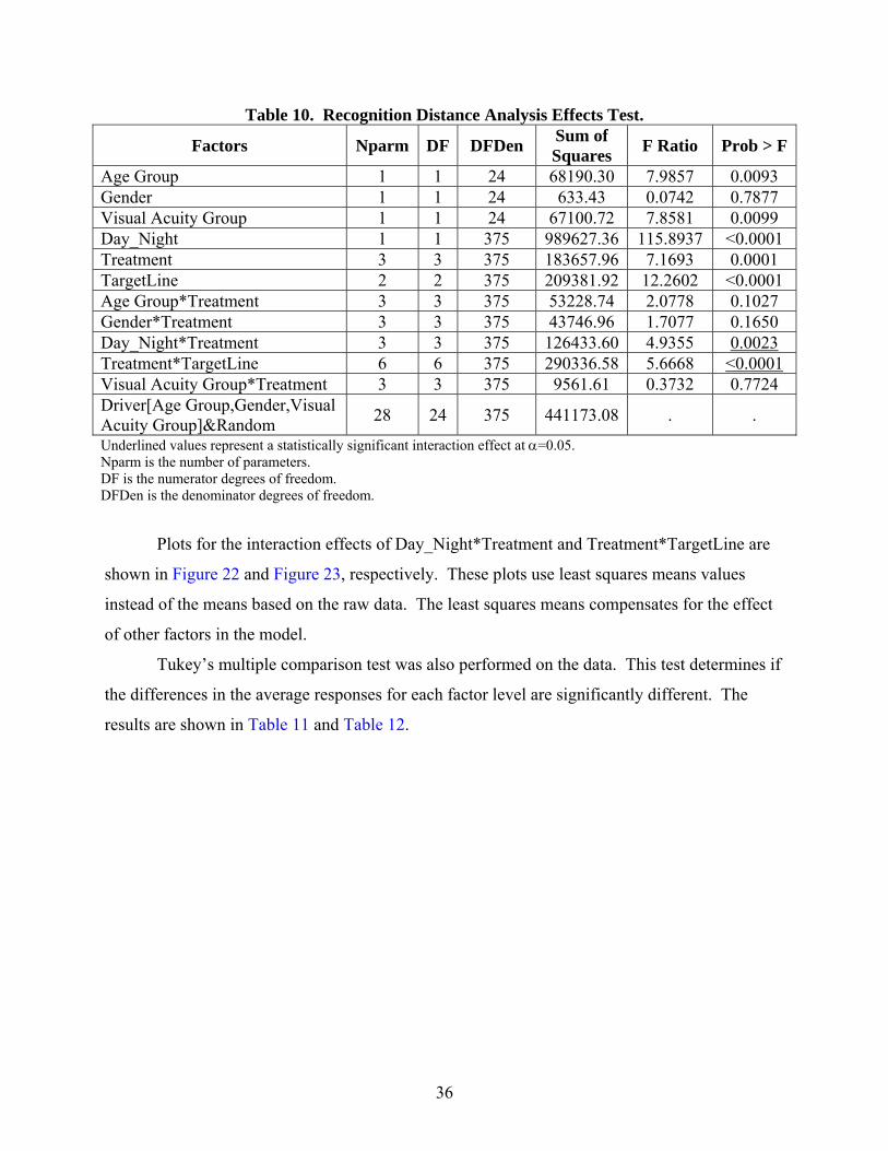
The results of the recognition distance analysis are shown in Table 9 and Table 10. The

results indicate significant interaction between font treatment (Treatment) and lighting level

(Day_Night) and also between font treatment and what line the sign legend was located on

(TargetLine).

Table 9. Recognition Distance Analysis Summary of Fit. R2 0.51819 R2

Adj 0.485586 Root Mean Square Error 92.40722 Mean of Response 482.3513 Observations 427

36

Table 10. Recognition Distance Analysis Effects Test.

Factors Nparm DF DFDen Sum of Squares F Ratio Prob > F

Age Group 1 1 24 68190.30 7.9857 0.0093 Gender 1 1 24 633.43 0.0742 0.7877 Visual Acuity Group 1 1 24 67100.72 7.8581 0.0099 Day_Night 1 1 375 989627.36 115.8937 <0.0001 Treatment 3 3 375 183657.96 7.1693 0.0001 TargetLine 2 2 375 209381.92 12.2602 <0.0001 Age Group*Treatment 3 3 375 53228.74 2.0778 0.1027 Gender*Treatment 3 3 375 43746.96 1.7077 0.1650 Day_Night*Treatment 3 3 375 126433.60 4.9355 0.0023 Treatment*TargetLine 6 6 375 290336.58 5.6668 <0.0001 Visual Acuity Group*Treatment 3 3 375 9561.61 0.3732 0.7724 Driver[Age Group,Gender,Visual Acuity Group]&Random 28 24 375 441173.08 . .

Underlined values represent a statistically significant interaction effect at α=0.05. Nparm is the number of parameters. DF is the numerator degrees of freedom. DFDen is the denominator degrees of freedom.

Plots for the interaction effects of Day_Night*Treatment and Treatment*TargetLine are

shown in Figure 22 and Figure 23, respectively. These plots use least squares means values

instead of the means based on the raw data. The least squares means compensates for the effect

of other factors in the model.

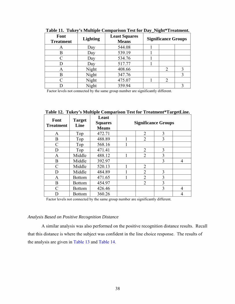
Tukey’s multiple comparison test was also performed on the data. This test determines if

the differences in the average responses for each factor level are significantly different. The

results are shown in Table 11 and Table 12.

37

Figure 22. Interaction Plot of Day_Night*Treatment.

Figure 23. Interaction Plot of Font Treatment*TargetLine.

0

100

200

300

400

500

600

700

A B C D

Font Treatment

Rec

ogni

tion

Dis

tanc

e (ft

)Le

ast S

quar

es M

eans

Day

Night

0

100

200

300

400

500

600

700

A B C D

Font Treatment

Rec

ogni

tion

Dis

tanc

e (ft

)Le

ast S

quar

e M

eans

Top

Middle

Bottom

38

Table 11. Tukey’s Multiple Comparison Test for Day_Night*Treatment. Font

Treatment Lighting Least Squares Means Significance Groups

A Day 544.08 1 B Day 539.19 1 C Day 534.76 1 D Day 517.77 1 A Night 408.66 2 3 B Night 347.76 3 C Night 475.07 1 2 D Night 359.94 3

Factor levels not connected by the same group number are significantly different.

Table 12. Tukey’s Multiple Comparison Test for Treatment*TargetLine.

Font Treatment

Target Line

Least Squares Means

Significance Groups

A Top 472.71 2 3 B Top 488.89 1 2 3 C Top 568.16 1 D Top 471.41 2 3 A Middle 488.12 1 2 3 B Middle 392.97 3 4 C Middle 520.13 1 2 D Middle 484.89 1 2 3 A Bottom 471.65 1 2 3 B Bottom 454.97 2 3 C Bottom 426.46 3 4 D Bottom 360.26 4


Analysis Based on Positive Recognition Distance

A similar analysis was also performed on the positive recognition distance results. Recall

that this distance is where the subject was confident in the line choice response. The results of

the analysis are given in Table 13 and Table 14.

39

Table 13. Postive Recognition Distance Analysis Summary of Fit.

R2 0.665262 R2

Adj 0.642611 Root Mean Square Error 67.09189 Mean of Response 375.9415 Observations (or Sum Weights) 427

Table 14. Postive Recognition Distance Analysis Effects Test.

Source Nparm DF DFDen Sum of Squares F Ratio Prob >

F Age Group 1 1 24 39775.04 8.8363 0.0066 Gender 1 1 24 1823.26 0.4050 0.5305 Visual Acuity Group 1 1 24 49180.98 10.9259 0.0030 Day_Night 1 1 375 909897.05 202.1400 <0.0001 Treatment 3 3 375 174743.63 12.9402 <0.0001 TargetLine 2 2 375 132004.08 14.6628 <0.0001 Age Group*Treatment 3 3 375 10542.47 0.7807 0.5053 Gender*Treatment 3 3 375 26537.72 1.9652 0.1188 Day_Night*Treatment 3 3 375 86060.52 6.3730 0.0003 Treatment*TargetLine 6 6 375 145880.24 5.4014 <0.0001 Visual Acuity Group*Treatment 3 3 375 1891.69 0.1401 0.9360 Driver[Age Group, Gender, Visual Acuity Group]&Random 28 24 375 498868.70 . .


Again, interaction effects of Day_Night*Treatment and Treatment*TargetLine are

significant. Plots of these interaction effects are shown in Figure 24 and Figure 25. Tukey’s

multiple comparison test was also applied to the interaction effects. The results of the Tukey’s

test are given in Table 15 and Table 16.

40


Figure 25. Interaction Plot of Treatment*TargetLine.

0

100

200

300

400

500

600

700

A B C D

Font Treatment

Posi

tive

Rec

ogni

tion

Dis

tanc

eLe

ast S

quar

e M

ean

Day

Night

0

100

200

300

400

500

600

700

A B C D

Font Treatment

Posi

tive

Rec

ogni

tion

Dis

tanc

eLe

ast S

quar

e M

eans

TopMiddleBottom

41

Table 15. Tukey’s Multiple Comparison Test for Day_Night*Treatment.

Font Treatment Lighting

Least Squares Means

Significance Groups

A Day 439.33 1 B Day 429.05 1 C Day 426.79 1 D Day 401.80 1 2 A Night 314.91 3 B Night 248.39 4 C Night 355.94 2 3 D Night 254.89 4


Table 16. Tukey’s Multiple Comparison Test for Treatment*TargetLine.

Font Treatment Line

Least Squares Means

Significance Groups

A Top 377.032 2 3 B Top 376.554 1 2 3 4 C Top 443.925 1 D Top 353.745 2 3 4 A Middle 372.958 1 2 3 4 B Middle 297.441 4 5 C Middle 397.554 1 2 D Middle 355.597 2 3 4 5 A Bottom 381.382 1 2 3 B Bottom 342.181 3 4 C Bottom 332.629 3 4 5 D Bottom 275.71 5


Legibility Task

In the analysis of the legibility task, the dependent variable is the calculated legibility

distance. There were 2,138 legibility measurements. Again, the experiment was a split-plot

design with subject gender and age grouping (younger and older) as whole plot factors. Time of

day (Day-Night), font treatment (Treatment), sign color (Color), number of lines of legend

(NumLine), and the particular line the subject was instructed to read (Target Line) were split-plot

factors. The results of the legibility analysis are given in Table 17 and Table 18.

42

Table 17. Legibility Analysis Summary of Fit. R2 0.63712 R2

Adj 0.632128 Root Mean Square Error 54.41674 Mean of Response 336.6791 Observations (or Sum Weights) 2138

Table 18. Legibility Analysis Effects Test.

Source Nparm DF DFDen Sum of Squares F Ratio Prob > F

Age_Group 1 1 27 34499.0 11.6504 0.0020 Gender 1 1 27 5616.5 1.8967 0.1798 Day_Night 1 1 2081 4177082.7 1410.614 <0.0001 Color 2 2 2081 188765.3 31.8733 <0.0001 Treatment 3 3 2081 130156.4 14.6514 <0.0001 NumLine 1 1 2081 30631.9 10.3445 0.0013 TargetLine 2 2 2081 4177.7 0.7054 0.4940 Age_Group*Treatment 3 3 2081 11821.9 1.3308 0.2626 Gender*Treatment 3 3 2081 7298.6 0.8216 0.4819 Day_Night*Treatment 3 3 2081 30735.7 3.4599 0.0158 Color*Treatment 6 6 2081 257098.0 14.4705 <0.0001 Treatment*NumLine 3 3 2081 50533.7 5.6885 0.0007 Driver[Age_Group,Gender]&Random 30 27 2081 3418465.6 . .


The effects tests show that there are significant interaction effects of Day_Night*

Treatment, Color*Treatment, and Treatment*NumLine. Interaction plots for these effects are

given in Figure 26 through Figure 28. Tukey’s multiple comparison tests were also performed,

and the results are shown in Table 19 through Table 21.

43


Figure 27. Interaction Plot of Treatment*NumLine.

0

100

200

300

400

500

600

700

A B C D

Font Treatment

Legi

bilit

y D

ista

nce

Leas

t Squ

are

Mea

nDay

Night

0

100

200

300

400

500

600

700

A B C DFont Treatment

Legi

bilit

y D

ista

nce

Leas

t Sqa

ure

Mea

ns

2-Line Legend3-Line Legend

44

Figure 28. Interaction Plot of Treatment*Color.

Table 19. Tukey’s Multiple Comparison Test for Day_Night*Treatment.

Font Treatment Lighting

Least Squares Means

Significance Groups

A Day 379.15 1 2 B Day 364.12 1 2 C Day 381.87 1 D Day 347.43 2 A Night 284.2 3 B Night 267.12 3 C Night 272.41 3 D Night 263.99 3


0

100

200

300

400

500

600

700

A B C DFont Treatment

Legi

bilit

y D

ista

nce

Leas

t Sqa

ure

Mea

nsFl. Yellow

Fl. Orange

White

45

Table 20. Tukey’s Multiple Comparison Test for Treatment*NumLine.

Font Treatment

Lines of Legend

Least Squares Means

Significance Groups

A 2 335.62 1 B 2 335.16 1 C 2 335.45 1 D 2 309.71 2 3 4 A 3 327.73 1 2 B 3 296.08 4 C 3 318.83 1 2 3 D 3 301.7 3 4


Table 21. Tukey’s Multiple Comparison Test for Treatment*Color.

Font Treatment Color

Least Squares Means

Significance Groups

A Fl. Yellow 341.65 1 B Fl. Yellow 318.75 2 3 C Fl. Yellow 335.32 1 2 D Fl. Yellow 337.91 1 2 A Fl. Orange 312.25 3 B Fl. Orange 311.39 3 4 C Fl. Orange 336.42 1 2 D Fl. Orange 289.23 4 A White 341.13 1 B White 316.72 2 3 C White 309.69 3 4 D White 289.97 4


47

CHAPTER 4: CONCLUSIONS

DISCUSSION

The following chapter discusses the results from the laptop evaluation and the field study.

Laptop Study

The initial evaluation in this project was a laptop study. The results from this effort

indicate that using a mixed case font such as Clearview does not significantly increase the

readability of a negative contrast sign when compared to the same sign in an all uppercase font.

Subjects showed similar correct response rates for each sign. The particular message appeared to

have more effect on readability than font. For the multiple choice portion of the laptop study, the

mixed case Clearview font did produce slightly higher recognition performance compared to the

all uppercase versions. If drivers are actively searching and anticipating possible messages on

signs given their trip destination and roadway context, a mixed case footprint may allow them to

more quickly identify their desired sign and extract the necessary information.

Field Study

The analysis of the field study was conducted in two parts. The first part examined the

descriptive statistics of the data to make a practical judgment on the benefit of the Clearview font

on negative contrast signs. The second part involved an in-depth statistical analysis examining

the various interactions between the factors of the experiment to determine if there was any

statistical significance to the results.

Recognition Distance

The recognition task was performed in order to determine if drivers benefit from the use

of an upper/lowercase font over that of an all-uppercase font when identifying a word (or

destination name in the case of guide signing) based on the word’s footprint. Main effect

variables such as age group, visual acuity, day versus night, treatments, and target line were all

identified as being statistically significant, as one might expect. The statistically significant

interactions are of particular interest here, however. For instance, in Figure 24 the interaction of

day-night and treatment is shown. During the daytime conditions there appears to be no

48

difference between any of the treatments. Additional statistical testing shown in Appendix E

confirms that all the fonts performed the same (i.e., were recognized at the same distance) during

the daytime conditions. The results during the nighttime conditions are more interesting. As

expected, the nighttime recognition distances are less than the daytime recognition distances.

More interesting, however, is the performance of the alternate fonts. The straight replacement of

the FHWA font with Clearview produced the worst overall nighttime recognition distance, both

quantitatively and statistically. From a statistical point of view, Treatments A and C can be

considered to perform the same, meaning the potential of the negative contrast version of

Clearview might not be obtained yet, and further redesign is needed

Legibility Distance

Like the recognition analysis, the legibility analysis shows that all the main effect

variables except gender are statistically significant. Daytime legibility distance is greater than

nighttime for all font treatments (see Figure 26). Further analysis by either day or night shows

that none of the font treatments was significantly different from the other (see Table 19). The

interaction effect between the lines of legend and font treatment (see Figure 27) shows that two-

line legend signs have a slightly higher legibility distance than three-line legend signs for

Treatment B. However, for both lengths of legend there is no significant difference between the

font treatments (see Table 20). When it comes to sign color, the results were mixed. For

fluorescent yellow signs, all the fonts performed statistically the same. For white signs, the

standard FHWA performed better than any of the alternates. For fluorescent orange signs,

Treatment C outperformed all other treatments. Table 21 reveals that no single font treatment

consistently outperforms the others as a function of sign color. Table 21 also shows that the

straight replacement of the FHWA font with the recommended Clearview font generally

provides one of the least legible scores within each sign color.

CONCLUSIONS

The research activities conducted to fulfill the objectives of this research project have led

to the following conclusions:

• The positive contrast version of Clearview underwent several modifications before it

was approved for use by the FHWA.

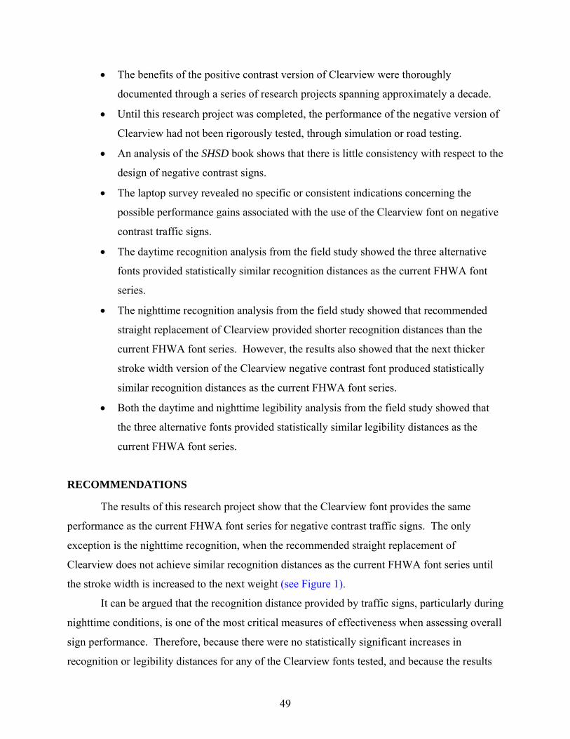
49

• The benefits of the positive contrast version of Clearview were thoroughly

documented through a series of research projects spanning approximately a decade.

• Until this research project was completed, the performance of the negative version of

Clearview had not been rigorously tested, through simulation or road testing.

• An analysis of the SHSD book shows that there is little consistency with respect to the

design of negative contrast signs.

• The laptop survey revealed no specific or consistent indications concerning the

possible performance gains associated with the use of the Clearview font on negative

contrast traffic signs.

• The daytime recognition analysis from the field study showed the three alternative

fonts provided statistically similar recognition distances as the current FHWA font

series.

• The nighttime recognition analysis from the field study showed that recommended

straight replacement of Clearview provided shorter recognition distances than the

current FHWA font series. However, the results also showed that the next thicker

stroke width version of the Clearview negative contrast font produced statistically

similar recognition distances as the current FHWA font series.

• Both the daytime and nighttime legibility analysis from the field study showed that

the three alternative fonts provided statistically similar legibility distances as the

current FHWA font series.

RECOMMENDATIONS

The results of this research project show that the Clearview font provides the same

performance as the current FHWA font series for negative contrast traffic signs. The only

exception is the nighttime recognition, when the recommended straight replacement of

Clearview does not achieve similar recognition distances as the current FHWA font series until

the stroke width is increased to the next weight (see Figure 1).

It can be argued that the recognition distance provided by traffic signs, particularly during

nighttime conditions, is one of the most critical measures of effectiveness when assessing overall

sign performance. Therefore, because there were no statistically significant increases in

recognition or legibility distances for any of the Clearview fonts tested, and because the results

50

of the nighttime recognition analysis showed an actual decrease in recognition distance when the

FHWA font was replaced with the recommended Clearview font, the researchers recommend

that TxDOT maintain its current practice of using the FHWA font series for negative contrast

signs.

In addition, the preliminary analysis using sign layout software indicated that the

substitution of the Clearview font would result in many standard signs exceeding the borders of

the current sign blank sizes. This analysis demonstrated that modifications and adjustments

would have to be made to each negative contrast sign (particularly warning and work zone signs)

on an individual basis to check for intrusion on the border.

FUTURE RESEARCH

Ideally a transportation agency would use one font style for all their traffic signs. In an

effort to move toward that goal, the researchers recommend that additional research be

conducted to test thicker stroke widths of the Clearview font for negative contrast signs. The

only condition in which the Clearview font did not perform at least statistically equivalently to

the current FHWA font series was nighttime recognition distances. However, when a heavier

weight Clearview was used in this condition, the recognition distances were increased and were

found to be statistically equal to those measured using the current FHWA font series. If the

additional research was successful in determining that the negative contrast version of Clearview

provided at least equivalent performance as the current FHWA font series, then the documented

increase in performance associated with the positive contrast version of Clearview might be

enough to justify transportation agencies to begin transitioning to one font style. Additional

research would also be needed to fit Clearview into the negative contrast signs while maintaining

equivalent performance. As demonstrated herein, this will be particularly challenging with

diamond-shaped warning and construction signs.

51

REFERENCES

1. Garvey, P.M., M.T. Pietrucha, and D. Meeker. Legibility of Guide Signs. In Transportation Research Record 1605, TRB, National Research Council, Washington, D.C., 1997, pp. 73-79.

2. Hawkins, H.G., M.D. Wooldridge, A.B. Kelly, D.L. Picha, and F.K. Greene. Legibility

Comparison of Three Freeway Guide Sign Alphabets, FHWA/TX-99/1276-1F, College Station, Texas, May 1999.

3. Carlson, P.J. Evaluation of Clearview Alphabet with Microprismatic Retroreflective

Sheeting, Report 4049-1, College Station, Texas, October 2001.

4. Holick, A., and P.J. Carlson. Nighttime Guide Sign Legibility for Microprismatic Clearview Legend on High Intensity Background, Report 1976-4, College Station, Texas, 2004.

5. TxDOT Memorandum, December 22, 2003.

6. Chrysler, S.T., P.J. Carlson, and H.G. Hawkins. Nighttime Legibility of Ground-Mounted

Traffic Signs as a Function of Font, Color, and Retroreflective Sheeting Type, FHWA/TX-02/1796-2, College Station, Texas, September 2002.

7. Zwahlen, H.T., and T. Schnell. Legibility of Traffic Sign Text and Symbols, In

Transportation Research Record 1692, TRB, National Research Council, Washington, D.C., 1999, pp. 142-151.

53

APPENDIX A LAPTOP EVALUATION STUDY SIGNS

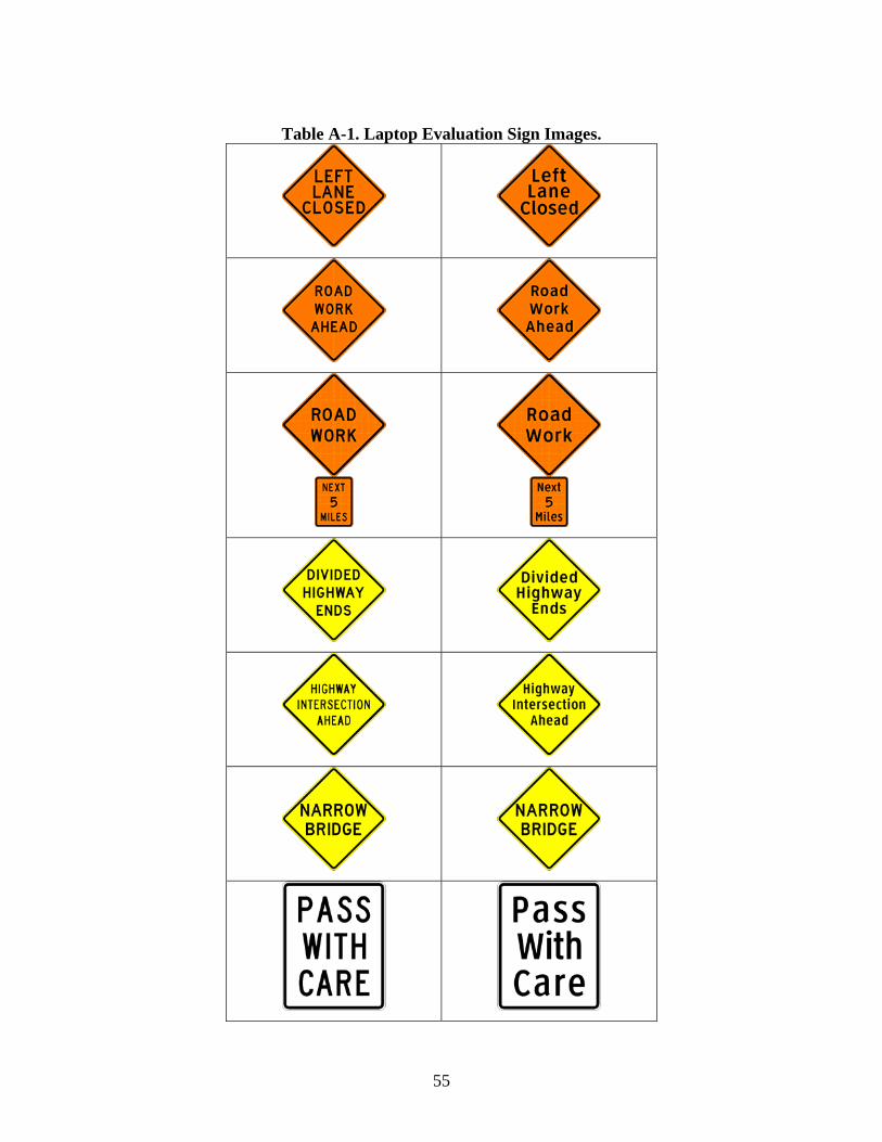
55

Table A-1. Laptop Evaluation Sign Images.

57

APPENDIX B PROJECT EVALUATION FIELD STUDY SIGN LAYOUTS

59

Regulatory Signs Used for Recognition Portion

Sign 1 Treatment A Standard all uppercase alphabet Highway C font 100% spacing

Sign 2 Treatment B Clearview upper/lowercase straight replacement Clearview Hwy 2-B font 100% spacing

Sign 3 Treatment C Increase the series of Clearview Clearview Hwy 3-B font 100% spacing

Sign 4 Treatment D Decrease inter-line spacing from 3" to 2.5" Clearview Hwy 2-B font 100% spacing

60

Regulatory Signs Used for Recognition Portion




Sign 8 Treatment D Decrease inter-line spacing from 3" to 2" Clearview Hwy 2-B font 100% spacing

61

Warning Signs Used for Legibility Portion

Sign 9 Treatment A Standard all uppercase alphabet Highway D font 100% spacing



Sign 12 Treatment D Increase inter-letter spacing Clearview Hwy 3-B font 200% spacing

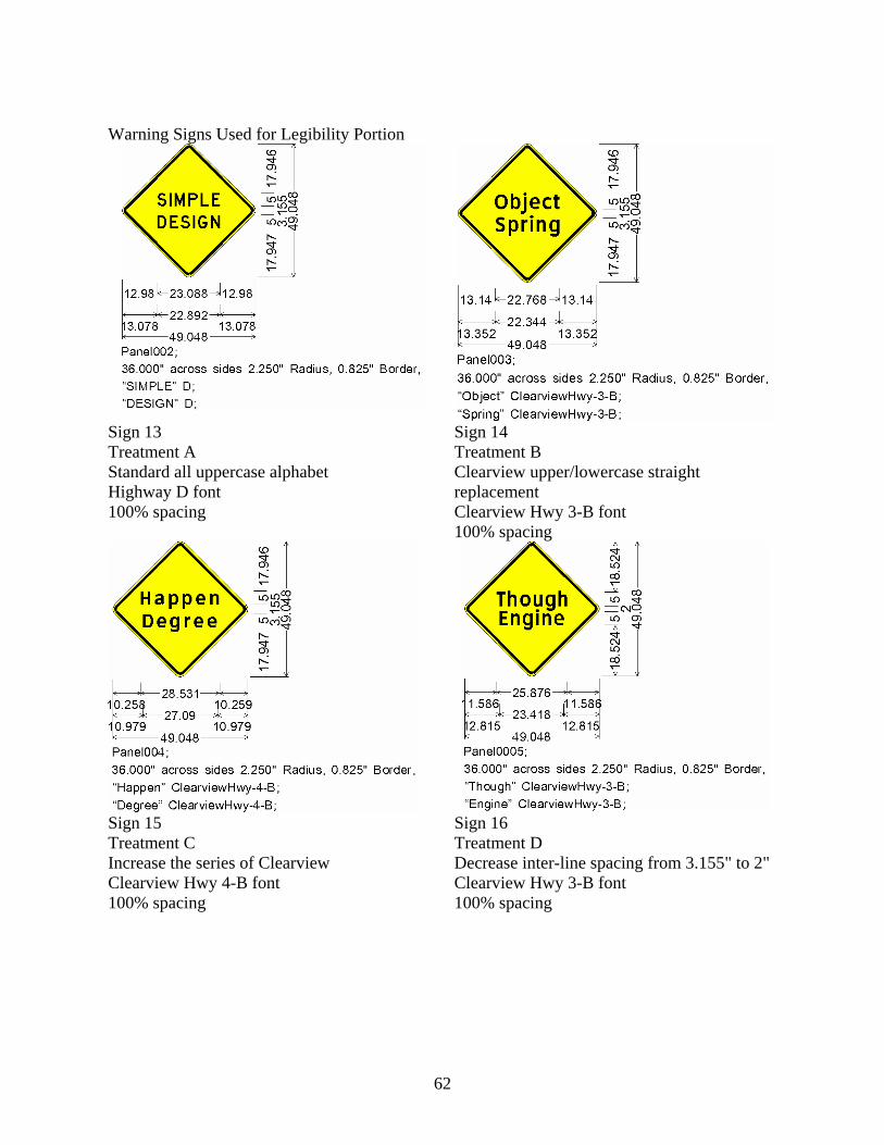
62





Sign 16 Treatment D Decrease inter-line spacing from 3.155" to 2" Clearview Hwy 3-B font 100% spacing

63





Sign 20 Treatment D Decrease inter-line spacing from 3.2" to 2.67" Clearview Hwy 2-B font 100% spacing

64

Construction Signs Used for Legibility Portion




Sign 24 Treatment D Increase inter-letter spacing Hwy 3-B font 200% spacing

65





Sign 28 Treatment D Decrease inter-line spacing from 4.02" to 3" Clearview Hwy 3-B font 100% spacing

66





Sign 32 Treatment D Decrease inter-line spacing from 3.4" to 2.25" Clearview Hwy 2-B font 100% spacing

67

Regulatory Signs Used for Legibility Portion



Sign 35 Treatment C Increase the Series of Clearview Clearview Hwy 3-B font 100% spacing

Sign 36 Treatment D Decrease top spacing from 10" to 8.25" Increase bottom spacing from 6.5" to 8.25" Clearview Hwy 2-B font 100% spacing

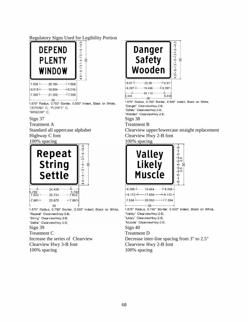
68





Sign 40 Treatment D Decrease inter-line spacing from 3" to 2.5" Clearview Hwy 2-B font 100% spacing

69





Sign 44 Treatment D Decrease inter-line spacing from 3" to 2" Clearview Hwy 2-B font 100% spacing

71

APPENDIX C RECOGNITION DATA CASE SUMMMARY

73

Table C-1. Recognition Data Case Summary, Day. Day

Younger Older White White

A B C D All Treatments A B C D All Treatments

N 45 46 46 45 182 14 14 14 14 56

Mean 611.09 554.87 596.8 527.47 572.59 446.43 475 550 440.93 478.09

Std. Deviation 112.389 96.296 79.126 111.782 105.231 92.952 80.264 116.024 105.312 106.271

Std. Error of Mean 16.754 14.198 11.666 16.663 7.8 24.843 21.451 31.009 28.146 14.201

Minimum 347 400 450 251 251 300 400 300 300 300

1st Quartile 600 500 513 464 400 400 500 400

Median 600 550 600 500 600 425 500 550 400 500

3rd Quartile 700 600 638 600 500 500 600 500

Maximum 900 800 800 700 900 600 700 700 700 700

Range 553 400 350 449 649 300 300 400 400 400

73

74

Table C-2. Recognition Data Case Summary, Night. Night



N 46 44 46 46 182 14 13 14 14 55

Mean 450.76 389.02 457.93 415.46 428.73 392.71 357.69 403.57 396.64 388.2

Std. Deviation 96.718 92.664 137.861 86.53 108.261 101.852 90.935 108.245 122.929 105.37

Std. Error of Mean 14.26 13.97 20.327 12.758 8.025 27.221 25.221 28.93 32.854 14.208

Minimum 300 250 250 200 200 248 250 200 200 200

1st Quartile 400 300 385 400 300 300 313 300

Median 500 400 400 400 400 400 300 400 400 400

3rd Quartile 500 400 500 500 400 400 500 500

Maximum 700 700 900 600 900 600 500 600 600 600

Range 400 450 650 400 700 352 250 400 400 400

74

75

Table C-3. Positive Recognition Data Case Summary, Day. Day



N 46 46 46 46 184 14 14 14 14 56

Mean 511.98 459.72 496.52 439.13 476.84 366.43 349.86 411.57 331.93 364.95

Std. Deviation 111.864 72 65.376 109.086 95.749 96.066 82.885 107.381 104.854 100.093

Std. Error of Mean 16.493 10.616 9.639 16.084 7.059 25.675 22.152 28.699 28.023 13.376

Minimum 341 300 348 251 251 206 250 233 175 175

1st Quartile 459 403 453 370 284 270 333 291

Median 498 463.5 498 428 469 369 354.5 377.5 313.5 359

3rd Quartile 560 502 546 487 411 405 476 400

Maximum 1,000 631 645 1,000 1,000 530 500 603 576 603

Range 659 331 297 749 749 324 250 370 401 428

75

76

Table C-4. Positive Recognition Data Case Summary, Night.

Night Younger Older

White White


N 46 46 46 46 184 14 14 14 14 56

Mean 342.35 327.07 349.46 295.43 328.58 303.93 307.93 290.21 287.57 297.41

Std. Deviation 68.975 160.568 100.738 63.74 106.95 87.57 228.021 81.919 107.537 136.009

Std. Error of Mean 10.17 23.675 14.853 9.398 7.884 23.404 60.941 21.894 28.741 18.175

Minimum 150 187 216 106 106 157 20 200 100 20

1st Quartile 310 246 295 261 240 204 231 229

Median 336.5 285.5 337 298.5 317 293.5 248.5 288 292 288.5

3rd Quartile 387 340 367 333 341 308 308 388

Maximum 500 1,000 800 419 1,000 510 1,000 500 431 1,000

Range 350 813 584 313 894 353 980 300 331 980

76

77

Table C-5. Recognition Case Summary, Collapsed Categories. All Younger

Drivers All Older Drivers All Drivers

N 364 111 475

Mean 500.66 433.55 484.98

Std. Deviation 128.664 114.61 128.586

Std. Error of Mean 6.744 10.878 5.9

Minimum 200 200 200

Median 500 400 500

Maximum 900 700 900

Range 700 500 700

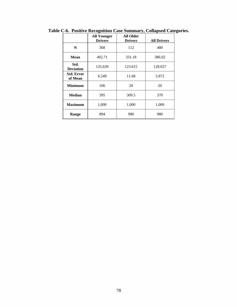
78

Table C-6. Positive Recognition Case Summary, Collapsed Categories. All Younger


N 368 112 480

Mean 402.71 331.18 386.02

Std. Deviation 125.639 123.615 128.657

Std. Error of Mean 6.549 11.68 5.872

Minimum 106 20 20

Median 395 309.5 370

Maximum 1,000 1,000 1,000

Range 894 980 980

79

APPENDIX D LEGIBILITY CASE SUMMARY

81

Table D-1. Legibility Case Summary, Younger Driver, Day. Day

Younger Fl. Orange Fl. Yellow White

A B C D All

Treatments A B C D All Treatments A B C D All

Treatments All

Colors

N 63 63 63 62 251 63 63 63 63 252 63 63 62 63 251 754

Mean 282.13 293.63 316.21 251.84 286.09 316.86 281.87 306.76 321.71 306.8 308.83 289.05 289.16 253.9 285.22 292.72

Median 286 291 317 245.5 289 323 284 306 334 317.5 302 294 287 255 283 294

Std. Error of Mean 7.42 8.84 8.57 9.13 4.48 9.26 11.26 9.21 9.32 4.97 10.82 8.31 7.51 7.31 4.47 2.7

Minimum 122 159 172 105 105 106 -33 79 51 -33 63 97 133 121 63 -33

Maximum 421 512 478 402 512 448 467 512 497 512 514 430 430 369 514 514

Range 299 353 306 297 407 342 500 433 446 545 451 333 297 248 451 547

Std. Deviation 58.88 70.18 68.01 71.87 70.90 73.48 89.35 73.09 73.98 78.83 85.898 65.97 59.1 58.02 70.65 74.14

81

82

Table D-2. Legibility Case Summary, Older Driver, Day. Day

Older Fl. Orange Fl. Yellow White

A B C D All


Treatments All

Colors

N 18 18 18 17 71 18 16 18 18 70 18 17 18 18 71 212

Mean 232.22 215.94 256.89 173.76 220.35 246.11 240.31 271.44 243.61 250.66 240.00 230.00 219.44 186.72 218.89 229.87

Median 255 217 259.5 179 216 269.5 221.5 291.5 251.5 261 277.5 229 239 199 230 230.5

Std. Error of Mean 19.91 19.02 26.84 17.76 11.01 15.93 21.39 16.42 18.28 8.90 20.41 18.35 19.71 17.01 9.57 5.76

Minimum 57 108 116 51 51 99 108 130 48 48 68 54 59 20 20 20

Maximum 356 380 630 330 630 326 381 367 376 381 347 331 356 293 356 630

Range 299 272 514 279 579 227 273 237 328 333 279 277 297 273 336 610

Std. Deviation 84.46 80.68 113.88 73.22 92.74 67.57 85.54 69.65 77.57 74.49 86.60 75.66 83.61 72.16 80.64 83.90

82

83

Table D-3. Legibility Case Summary, Younger Driver, Night. Night

Younger Fl. Orange Fl. Yellow White

A B C D All


Treatments All

Colors

N 71 72 72 66 281 71 72 70 72 285 853 71 72 72 66 281

Mean 213.87 207.46 201.96 206.45 207.43 203.45 173.88 160.03 174.56 178.01 191.65 213.87 207.46 201.96 206.45 207.43

Median 211 216 208 216.5 212 219 179.5 167.5 169.5 180 195 211 216 208 216.5 212

Std. Error of Mean 6.77 9.82 6.87 8.33 4.01 8.34 6.97 8.73 6.82 3.96 2.25 6.77 9.82 6.87 8.33 4.01

Minimum 86 10 -55 43 -55 -70 59 -35 8 -70 -70 86 10 -55 43 -55

Maximum 374 560 306 366 560 342 322 343 302 343 560 374 560 306 366 560

Range 288 550 361 323 615 412 263 378 294 413 630 288 550 361 323 615

Std. Deviation 57.04 83.33 58.26 67.68 67.20 70.24 59.17 73.02 57.83 66.87 65.60 57.04 83.33 58.26 67.68 67.20

83

84

Table D-4. Legibility Case Summary, Older Driver, Night. Night Older

Fl. Orange Fl. Yellow White

A B C D All


Treatments All

Colors

N 19 21 21 21 82 21 21 21 20 83 21 20 21 21 83 248

Mean 218.00 164.76 191.57 159.38 182.59 185.24 211.95 204.43 181.45 195.94 188.86 145.65 138.52 135.38 152.18 176.88

Median 168 163 165 129 162.5 171 187 187 181.5 181 182 142.5 137 136 157 162

Std. Error of Mean 43.01 22.50 29.49 30.43 15.73 15.09 30.21 32.51 12.58 12.10 16.48 11.11 14.01 13.07 7.21 7.09

Minimum 72 5 54 -18 -18 82 64 6 87 6 14 68 44 33 14 -18

Maximum 734 509 722 673 734 308 665 786 302 786 322 244 254 231 322 786

Range 662 504 668 691 752 226 601 780 215 780 308 176 210 198 308 804

Std. Deviation 187.50 103.11 135.12 139.44 142.42 69.15 138.43 148.96 56.26 110.23 75.54 49.70 64.19 59.87 65.71 111.61

84

85

Table D-5. Legibility Data Case Summary, Collapsed Categories. All Younger


N 1,607 460 2,067

Mean 239.07 201.30 230.67

Median 235.00 188.50 228.00

Std. Error of Mean 2.15 4.81 2.01

Minimum -70 -18 -70

Maximum 560 786 786

Range 630 804 856

Std. Deviation 86.06 103.14 91.47

87

APPENDIX E FIELD STUDY STATISTICAL ANALYSIS

89

EXPERIMENT DATA SUMMARY

The objective of this study was to determine if font and/or color affects sign recognition

and legibility. Two experiments were conducted, one for recognition test and the other for

legibility test. For recognition test, the dependent variables are Rec_Dist and Pos_Rec, and the

factor of main interest is Font having four levels: A, B, C, and D. For the legibility test, the

dependent variable is Adjusted Leg_Dist, and the factors of main interest are Font (having four

levels: A, B, C, and D) and Color (having three levels: Yellow, Orange, and White).

The experiments were conducted utilizing the split-plot design with Subject (driver) as a

whole plot and each treatment combination as a split plot. The demographic variables on subject

such as Gender, Age Group, Visual Acuity, and/or Contrast Sensitivity serve as whole-plot

factors, and the variables Day_Night, Font, Target Line, NumLine, and/or Color serve as split-

plot factors.

There were 30 subjects (drivers) involved in this study. The drivers can be treated as a

random factor in a split-plot model. The distribution of the whole-plot factors, Gender, Age

Group, Visual Acuity, and Contrast Sensitivity, are shown at the end of this appendix. Out of 30

drivers, 14 were females and 16 were males. Seven drivers belonged to the Old group (defined

by older than 55), and the remaining 23 drivers belonged to the Young group. Visual Acuity was

missing for three drivers. There were only 6 different measured values for Visual Acuity, with

20 (i.e., 20/20 visual acuity) as its mode (12 out of 30 drivers have 20). Contrast Sensitivity was

missing for 10 drivers. For the remaining 20 drivers, the value of contrast sensitivity ranged

from 31 to 64. After examining these distributions, the variables Visual Acuity and Contrast

Sensitivity were categorized as shown in Table E-1 for the purpose of making the analyses

feasible and facilitating the interpretation of the results. The categories were selected based on a

natural gap in the data.

90

Table E-1. Categorization of Variables Visual Acuity and Contrast Sensitivity.

Value of the original variable

Levels for the new variable: Visual Acuity Group

# of drivers in each group

Total number of drivers with a non-

missing value Visual Acuity

13~18 20~27

VA1 VA2

12 15 27

Contrast Sensitivity

31~45 48~53 57~64

CS1 CS2 CS3

10 5 5

20

ANALYSIS BASED ON RECOGNITION TASK DATA

In this analysis, the candidate dependent variables were recognition distance of the word

and line choice (Rec_Dist) and positive recognition distance of word and line choice (Pos_Rec).

A split-plot model having Gender, Age Group, and Visual Acuity Group (and/or Contrast

Sensitivity Group) as whole-plot factors along with Drivers as a nested random effect (nested

within Gender, Age Group, Visual Acuity Group, and/or Contrast Sensitivity Group), and

Day_Night, Treatment (here Font), and Target Line as split-plot factors was applied to each of

the datasets consisting of 480 measurements on Rec_Dist and Pos_Rec, respectively. Because

including Contrast Sensitivity in the analysis eliminates one-third of the observations in the data

(due to missing values), a model without Contrast Sensitivity Group and a model with Contrast

Sensitivity Group was applied separately to each of Rec_Dist and Pos_Rec.

Analysis Based on Rec_Dist

In addition to the main effects defined from the whole-plot factors and the split-plot

factors, the two-way interaction effects between Treatment and other factors were also included

in the model. Not all the two-way interaction effects or higher-order interaction effects could be

included due to the lack of degrees of freedom (i.e., there were not enough observations to test

all of those effects).

Model A

Model A is a model having Gender, Age Group, and Visual Acuity Group as whole-plot

factors, Driver as a random effect, and Day_Night, Font, and Target Line as split-plot factors as

well as all two-way interaction effects between Treatment and the other factors.

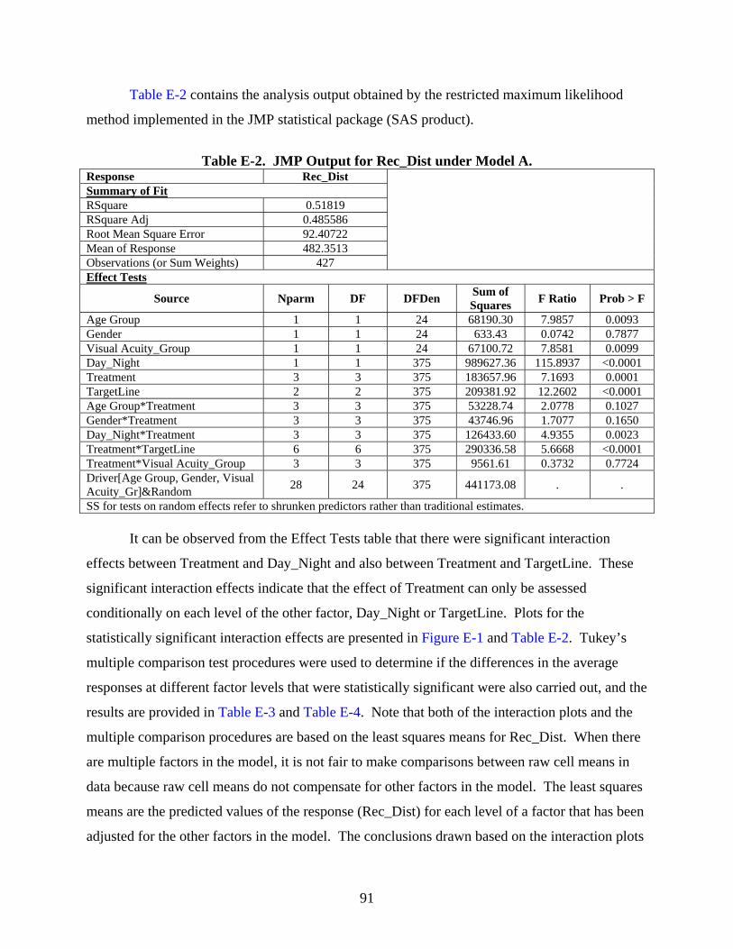
91

Table E-2 contains the analysis output obtained by the restricted maximum likelihood

method implemented in the JMP statistical package (SAS product).

Table E-2. JMP Output for Rec_Dist under Model A.

Response Rec_Dist Summary of Fit RSquare 0.51819 RSquare Adj 0.485586 Root Mean Square Error 92.40722 Mean of Response 482.3513 Observations (or Sum Weights) 427

Effect Tests


Age Group 1 1 24 68190.30 7.9857 0.0093 Gender 1 1 24 633.43 0.0742 0.7877 Visual Acuity_Group 1 1 24 67100.72 7.8581 0.0099 Day_Night 1 1 375 989627.36 115.8937 <0.0001 Treatment 3 3 375 183657.96 7.1693 0.0001 TargetLine 2 2 375 209381.92 12.2602 <0.0001 Age Group*Treatment 3 3 375 53228.74 2.0778 0.1027 Gender*Treatment 3 3 375 43746.96 1.7077 0.1650 Day_Night*Treatment 3 3 375 126433.60 4.9355 0.0023 Treatment*TargetLine 6 6 375 290336.58 5.6668 <0.0001 Treatment*Visual Acuity_Group 3 3 375 9561.61 0.3732 0.7724 Driver[Age Group, Gender, Visual Acuity_Gr]&Random 28 24 375 441173.08 . .

SS for tests on random effects refer to shrunken predictors rather than traditional estimates.

It can be observed from the Effect Tests table that there were significant interaction

effects between Treatment and Day_Night and also between Treatment and TargetLine. These

significant interaction effects indicate that the effect of Treatment can only be assessed

conditionally on each level of the other factor, Day_Night or TargetLine. Plots for the

statistically significant interaction effects are presented in Figure E-1 and Table E-2. Tukey’s

multiple comparison test procedures were used to determine if the differences in the average

responses at different factor levels that were statistically significant were also carried out, and the

results are provided in Table E-3 and Table E-4. Note that both of the interaction plots and the

multiple comparison procedures are based on the least squares means for Rec_Dist. When there

are multiple factors in the model, it is not fair to make comparisons between raw cell means in

data because raw cell means do not compensate for other factors in the model. The least squares

means are the predicted values of the response (Rec_Dist) for each level of a factor that has been

adjusted for the other factors in the model. The conclusions drawn based on the interaction plots

92

and the multiple comparison procedures are presented right after the multiple comparison test

tables.

R

ec_D

istL

S M

eans

300

400

500

600

Day

Night

A B C D

Treatment

Figure E-1. Interaction Plot for Day_Night*Treatment.

Table E-3. Tukey’s Multiple Comparison Test for Day_Night*Treatment. Level Least Sq. Mean Std. Error

Day, A A 544.08117 19.005417 Day, B A 539.19051 19.177954 Day, C A 534.76125 18.994030 Day, D A 517.76640 19.026583

Night, C A B 475.07370 18.978796 Night, A B C 408.65564 18.987111 Night, D C 359.93960 19.014254 Night, B C 347.76465 19.162469

The effect of Treatment on Rec_Dist is different for Day and Night. During Day, there is

no significant difference in the least squares mean Rec_Dist across the levels of Treatment (i.e.,

there is no Treatment effect during Day). During Night, however, Treatment C is significantly

different from Treatment B and D (i.e., Treatment C leads to a significantly larger least squares

mean Rec_Dist than Treatments B or D do) although there is still no significant difference

between Treatments C and A.

93

Figure E-2. Interaction Plot for Treatment*TargetLine.

Table E-4. Tukey’s Multiple Comparison Test for Treatment*TargetLine. Level Least Sq. Mean Std. Error C, Top A 568.16439 24.256759

C, Middle A B 520.12735 16.496290 D, Middle A B C 484.88986 24.256841 A, Middle A B C 484.74687 24.264105

B, Top A B C 482.49690 25.178314 A, Top B C 472.70983 16.507090

A, Bottom A B C 471.64851 24.444480 D, Top B C 471.40838 16.496411

B, Bottom B C 454.96792 16.543822 C, Bottom C D 426.46069 24.256759 B, Middle C D 392.96792 24.289109 D, Bottom D 360.26076 24.513181

The effect of TargetLine is different for each Treatment. For Treatment A, the predicted

mean Rec_Dist does not change significantly across the levels of TargetLine (i.e., no significant

effect of TargetLine is observed for Treatment A). The same can be said for Treatment B. For

Treatment C or D, however, there is a statistically significant effect of TargetLine on predicted

mean Rec_Dist. For example, for Treatment C, Top and Middle TargetLines lead to higher

predicted mean Rec_Dist than Bottom TargetLine does.

Because the interaction effects of Age Group*Treatment, Gender*Treatment, and

Treatment*Visual Acuity Group in Table E-2 are not statistically significant, the individual

effects of Age Group, Gender, and/or Visual Acuity on Rec_Dist can be assessed. It can be

Rec

_Dis

tLS

Mea

ns

300

400

500

600

A B

C

D

Bottom Middle Top TargetLine

94

concluded based on the p-values for Age Group, Gender, and/or Visual Acuity that Age Group

and Visual Acuity have statistically significant effects on Rec_Dist at the significance level

α=0.05 while the effect of Gender is not statistically significant.

Model B

Model B is a model having Gender, Age Group, Visual Acuity Group, and Contrast

Sensitivity Group as whole-plot factors, Driver as a random effect, and Day_Night, Font, and

Target Line as split-plot factors along with all two-way interaction effects between Treatment

and other factors

Table E-5 contains the analysis output obtained by the RML method under Model B

implemented in JMP.

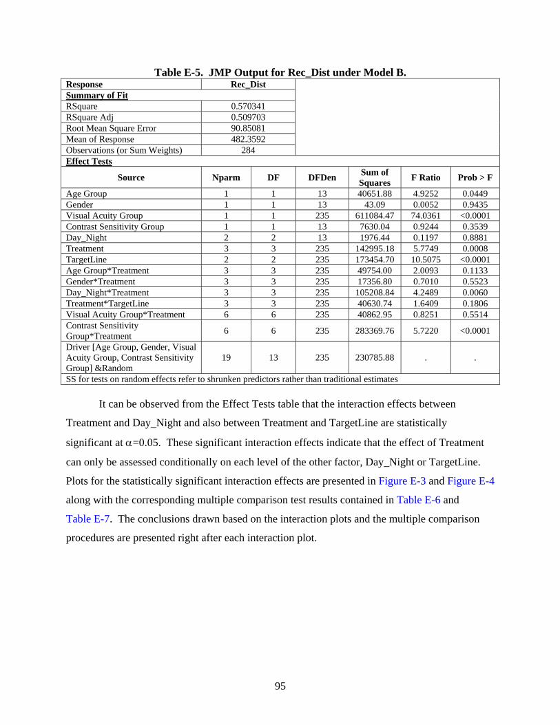
95

Table E-5. JMP Output for Rec_Dist under Model B. Response Rec_Dist Summary of Fit RSquare 0.570341 RSquare Adj 0.509703 Root Mean Square Error 90.85081 Mean of Response 482.3592 Observations (or Sum Weights) 284

Effect Tests


Age Group 1 1 13 40651.88 4.9252 0.0449 Gender 1 1 13 43.09 0.0052 0.9435 Visual Acuity Group 1 1 235 611084.47 74.0361 <0.0001 Contrast Sensitivity Group 1 1 13 7630.04 0.9244 0.3539 Day_Night 2 2 13 1976.44 0.1197 0.8881 Treatment 3 3 235 142995.18 5.7749 0.0008 TargetLine 2 2 235 173454.70 10.5075 <0.0001 Age Group*Treatment 3 3 235 49754.00 2.0093 0.1133 Gender*Treatment 3 3 235 17356.80 0.7010 0.5523 Day_Night*Treatment 3 3 235 105208.84 4.2489 0.0060 Treatment*TargetLine 3 3 235 40630.74 1.6409 0.1806 Visual Acuity Group*Treatment 6 6 235 40862.95 0.8251 0.5514 Contrast Sensitivity Group*Treatment 6 6 235 283369.76 5.7220 <0.0001

Driver [Age Group, Gender, Visual Acuity Group, Contrast Sensitivity Group] &Random

19 13 235 230785.88 . .

SS for tests on random effects refer to shrunken predictors rather than traditional estimates

It can be observed from the Effect Tests table that the interaction effects between

Treatment and Day_Night and also between Treatment and TargetLine are statistically

significant at α=0.05. These significant interaction effects indicate that the effect of Treatment

can only be assessed conditionally on each level of the other factor, Day_Night or TargetLine.

Plots for the statistically significant interaction effects are presented in Figure E-3 and Figure E-4

along with the corresponding multiple comparison test results contained in Table E-6 and

Table E-7. The conclusions drawn based on the interaction plots and the multiple comparison

procedures are presented right after each interaction plot.

96


Table E-6. Tukey’s Multiple Comparison Test for Day_Night*Treatment.

Level Least Sq. Mean Std. Error Day, B A 544.64336 24.252452 Day, A A 544.34841 24.040050 Day, C A 539.36212 23.884904 Day, D A 517.13778 23.884904

Night, C A B 490.68762 23.836442 Night, A B C 423.53192 23.972546 Night, D C 353.46803 23.836442 Night, B C 352.29477 24.219624

The effect of Treatment on Rec_Dist is different for Day and Night. During Day, there is

no significant difference in the predicted mean Rec_Dist across the levels of Treatment (i.e.,

there is no Treatment effect during Day). During Night, however, Treatment C is significantly

different from Treatments B and D (i.e., Treatment C leads to significantly larger predicted mean

Rec_Dist than Treatments B or D do) although there is still no significant difference between

Treatments C and A.

Rec

_Dis

tLS

Mea

ns

300

350

400

450

500

550

600

650

Day

Night

A B C D

Treatment

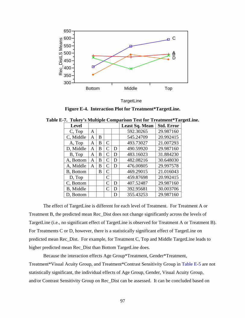
97

Rec

_Dis

tLS

Mea

ns

300350

400450

500550

600650

AB

C

D

Bottom Middle Top

TargetLine


Table E-7. Tukey’s Multiple Comparison Test for Treatment*TargetLine. Level Least Sq. Mean Std. Error C, Top A 592.30265 29.987160

C, Middle A B 545.24709 20.992415 A, Top A B C 493.73027 21.007293

D, Middle A B C D 490.59920 29.987160 B, Top A B C D 483.16023 31.884230

A, Bottom A B C D 482.08216 30.648030 A, Middle A B C D 476.00805 29.997578 B, Bottom B C 469.29015 21.016043

D, Top C 459.87698 20.992415 C, Bottom C D 407.52487 29.987160 B, Middle C D 392.95681 30.003706 D, Bottom D 355.43253 29.987160

The effect of TargetLine is different for each level of Treatment. For Treatment A or

Treatment B, the predicted mean Rec_Dist does not change significantly across the levels of

TargetLine (i.e., no significant effect of TargetLine is observed for Treatment A or Treatment B).

For Treatments C or D, however, there is a statistically significant effect of TargetLine on

predicted mean Rec_Dist. For example, for Treatment C, Top and Middle TargetLine leads to

higher predicted mean Rec_Dist than Bottom TargetLine does.

Because the interaction effects Age Group*Treatment, Gender*Treatment,

Treatment*Visual Acuity Group, and Treatment*Contrast Sensitivity Group in Table E-5 are not

statistically significant, the individual effects of Age Group, Gender, Visual Acuity Group,

and/or Contrast Sensitivity Group on Rec_Dist can be assessed. It can be concluded based on

98

the p-values for Age Group, Gender, Acuity Group, and/or Contrast Sensitivity Group that Age

Group has a statistically significant effect on Rec_Dist at the significance level α=0.05, while the

effects of Gender, Visual Acuity Group, and Contrast Sensitivity Group are not statistically

significant. It needs to be remembered that in this case the dataset itself (not just the model) is

different because all of the observations having missing Contrast Sensitivity have been removed

from the analysis. The filtering of Contrast Sensitivity may explain why the conclusion for the

effect of Visual Acuity Group is different from the previous case.

Analysis Based on Pos_Rec

The analyses are repeated for Pos-Rec under Model A and Model B defined previously.

Table E-8 contains the analysis output obtained by the restricted maximum likelihood method

implemented in the JMP statistical package.

Table E-8. JMP Output for Pos_Rec under Model A. Response Pos_Rec Summary of Fit RSquare 0.476936 RSquare Adj 0.441979 Root Mean Square Error 97.15292 Mean of Response 383.1644 Observations (or Sum Weights) 432

Effect Tests


Age Group 1 1 24 73831.26 7.8222 0.0100 Gender 1 1 24 3236.88 0.3429 0.5636 Visual Acuity_Group 1 1 24 86776.95 9.1937 0.0057 Day_Night 1 1 380 922714.18 97.7587 <0.0001 Treatment 3 3 380 114230.35 4.0341 0.0076 TargetLine 2 2 380 210527.27 11.1524 <0.0001 Age Group*Treatment 3 3 380 15370.75 0.5428 0.6533 Gender*Treatment 3 3 380 6120.38 0.2161 0.8852 Day_Night*Treatment 3 3 380 85472.45 3.0185 0.0298 Treatment*TargetLine 6 6 380 236749.78 4.1805 0.0004 Treatment*Visual Acuity_Group 3 3 380 15214.82 0.5373 0.6570 Driver [Age Group, Gender, VisualAcuity_Group]&Random 28 24 380 466277.78 . .


It can be observed from the Effect Tests table that there are significant interaction effects

between Treatment and Day_Night, and also between Treatment and TargetLine. These

significant interaction effects indicate that the effect of Treatment can only be assessed

99

conditionally on each level of the other factor Day_Night or TargetLine. Plots for the

statistically significant interaction effects and the corresponding multiple comparison test results

are presented in Figure E-5, Figure E-6, Table E-9, and Table E-10, respectively. The

conclusions drawn based on the interaction plots and the multiple comparison test procedures are

presented right after the multiple comparison test tables.


Table E-9. Tukey’s Multiple Comparison Test for Day_Night*Treatment. Level Least Sq. Mean Std. Error Day, B A 459.26702 19.871145 Day, A A 443.56156 19.871145 Day, C A B 427.13935 19.871145 Day, D A B 409.05848 19.871145

Night, C B C 355.58727 19.855090 Night, A C D 317.85203 19.855090 Night, B D 278.14433 19.855090 Night, D D 261.86631 19.855090

The effect of Treatment on Pos_Rec is different for Day and Night. During Day, there is

no significant difference in the predicted mean Pos_Rec across the levels of Treatment (i.e., there

is no Treatment effect during Day). During Night, however, Treatment C is significantly


Pos_Rec than Treatments B or D do) although there is still no significant difference between

Treatment C and A.

Pos

_Rec

LS M

eans

200250300350400450500

Day

Night

A B C D

Treatment

100


Table E-10. Tukey’s Multiple Comparison Test for Treatment*TargetLine. Level Least Sq. Mean Std. Error B, Top A 459.24888 25.425785 C, Top A B 443.91887 25.425785

A, Bottom A B C D 399.07716 25.425785 C, Middle A B C 397.54849 17.230479

A, Top A B C D 373.55865 17.230479 A, Middle A B C D 369.48457 25.425785 D, Middle A B C D 355.19079 25.425785

D, Top B C D 353.33894 17.230479 B, Bottom C D 345.80444 17.230479 C, Bottom B C D 332.62257 25.425785 B, Middle D 301.06370 25.425785 D, Bottom D 297.85746 25.425785

The effect of TargetLine on Pos_Rec is different for each level of Treatment. For

Treatments A, C, and D, the predicted mean Pos_Rec does not change significantly across the

levels of TargetLine (i.e., no significant effect of TargetLine is observed for Treatments A, C,

and D). For Treatment B, however, there is a statistically significant effect of TargetLine on

predicted mean Pos_Rec. Top TargetLine Treatment B leads to significantly higher predicted

mean Pos_Rec than Middle TargetLine Treatment B or Bottom TargetLine Treatment B does.

Because the interaction effects Age Group*Treatment, Gender*Treatment, and


effects of Age Group, Gender, and/or Visual Acuity on Pos_Rec can be assessed. It can be

Pos

_Rec

LS M

eans

200

250

300

350

400

450

500

A

BC

D

Bottom Middle Top

TargetLine

101

concluded based on the p-values for Age Group, Gender, and Visual Acuity Group that Age

Group and Visual Acuity have statistically significant effects on Pos_Rec at the significance

level α=0.05 while the effect of Gender is not statistically significant.


method under Model B implemented in JMP.

Table E-11. JMP Output for Rec_Dist under Model B. Response Pos_Rec Summary of Fit RSquare 0.483584 RSquare Adj 0.411859 Root Mean Square Error 106.0309 Mean of Response 380.4271 Observations (or Sum Weights) 288

Effect Tests


Age Group 1 1 13 24875.01 2.2126 0.1607 Gender 1 1 13 0.00462864 0.0000 0.9995 Day_Night 1 1 13 7848.78 0.6981 0.4185 Treatment 1 1 239 593918.56 52.8277 <0.0001 TargetLine 3 3 239 114216.80 3.3864 0.0188 Age Group*Treatment 2 2 239 228947.20 10.1822 <0.0001 Gender*Treatment 3 3 239 2363.14 0.0701 0.9759 Day_Night*Treatment 3 3 239 3028.91 0.0898 0.9656 Contrast Sensitivity Group 3 3 239 87816.50 2.6037 0.0526 Treatment*Contrast Sensitivity Group 2 2 13 17446.56 0.7759 0.4805

Treatment*TargetLine 6 6 239 28115.47 0.4168 0.8675 Visual Acuity Group 6 6 239 239023.29 3.5434 0.0022 Treatment*Visual Acuity Group 3 3 239 36972.96 1.0962 0.3514 Driver[Age Group, Gender, Contrast Sensitivity Group, Visual Acuity Group]&Random

19 13 239 314421.94 . .


It can be observed from the Effect Tests table that the interaction effect between

Treatment and TargetLine is statistically significant at α=0.05. Thus, the effect of Treatment can

only be assessed conditionally on each level of TargetLine and vice versa. Figure E-7 and

Table E-12 contain the interaction plot for Treatment*TargetLine and the corresponding multiple

comparison test results, respectively.

102


Table E-12. Tukey’s Multiple Comparison Test for Treatment*TargetLine. Level Least Sq. Mean Std. Error B, Top A 500.47021 35.063014 C, Top A B 460.88893 35.063014

A, Bottom A B C 418.79349 35.063014 C, Middle A B C 404.44448 24.593256

A, Top A B C 398.84904 24.593256 A, Middle A B C 388.68238 35.063014 D, Middle A B C 362.21449 35.063014

D, Top B C 350.82560 24.593256 B, Bottom B C 348.47021 24.593256 C, Bottom B C 331.66670 35.063014 B, Middle C 293.85910 35.063014 D, Bottom C 285.43671 35.063014

The effect of TargetLine on Pos_Rec is different for each level of Treatment. For

Treatments A, C, and D, the predicted mean Pos_Rec does not change significantly across the

levels of TargetLine (i.e., no significant effect of TargetLine is observed for Treatments A, C,

and D). For Treatment B, however, there is a statistically significant effect of TargetLine on

predicted mean Pos_Rec. Top TargetLine Treatment B leads to significantly higher predicted

mean Pos_Rec than Middle TargetLine Treatment B or Bottom TargetLine Treatment B does.


Treatment*Visual Acuity Group, and Treatment*Contrast Sensitivity Group,

Day_Night*Treatment in Table E-11 are not statistically significant, the individual effects of

Pos

_Rec

LS M

eans

200250300350400

500550600

A

BC

D

Bottom Middle Top

TargetLine

103

Age Group, Gender, Visual Acuity Group, Contrast Sensitivity Group, and Day_Night on

Pos_Rec can be assessed. It can be concluded based on the p-values for Age Group, Gender,

Acuity Group, Contrast Sensitivity Group, and Day_Night that the effect of Day_Night on

Pos_Rec is statistically significant at α=0.05, while none of Age Group, Gender, Visual Acuity

Group, and Contrast Sensitivity Group have statistically significant effects.

Notice that the conclusions obtained based on the Pos_Rec data are somewhat different

from those based on the Rec_Dist data. The patterns of the interaction plots in Figure E-6 and

Figure E-7 are different from those of Figure E-2 and Figure E-4, especially for Treatment B at

TargetLine Top. It was suspected that the outliers caused those significance differences. The

examination of the residual plot revealed the existence of five outliers, all having measured

values of 1,000 for Pos_Rec. Those outliers correspond to the observation ID numbers 173, 273,

305, 364, and 401. To see if the removal of those outliers will make a significant difference in

conclusions, those five observations are eliminated from the Pos_Rec data and the analysis is

rerun. For those five observations, the value of Rec_Dist is missing, which automatically

removes those five observations from the Rec_Dist data analysis.

Table E-13 contains the analysis output without the five outliers, obtained by the

restricted maximum likelihood method implemented in the JMP statistical package.

104

Table E-13. JMP Output for Pos_Rec under Model A without Five Outliers. Response Pos_Rec Summary of Fit RSquare 0.665262 RSquare Adj 0.642611 Root Mean Square Error 67.09189 Mean of Response 375.9415 Observations (or Sum Weights) 427

Effect Tests


Age Group 1 1 24 39775.04 8.8363 0.0066 Gender 1 1 24 1823.26 0.4050 0.5305 Visual Acuity Group 1 1 24 49180.98 10.9259 0.0030 Day_Night 1 1 375 909897.05 202.1400 <0.0001 Treatment 3 3 375 174743.63 12.9402 <0.0001 TargetLine 2 2 375 132004.08 14.6628 <0.0001 Age Group*Treatment 3 3 375 10542.47 0.7807 0.5053 Gender*Treatment 3 3 375 26537.72 1.9652 0.1188 Day_Night*Treatment 3 3 375 86060.52 6.3730 0.0003 Treatment*TargetLine 6 6 375 145880.24 5.4014 <0.0001 Visual Acuity Group*Treatment 3 3 375 1891.69 0.1401 0.9360 Driver[Age Group, Gender, Visual Acuity Group]&Random 28 24 375 498868.70 . .


Note that the R-square value increased significantly compared to the analysis with

outliers. There are significant interaction effects between Treatment and Day_Night and also

between Treatment and TargetLine. Plots for the statistically significant interaction effects and

the corresponding multiple comparison test results are presented in Figure E-8, Figure E-9,

Table E-14, and Table E-15, respectively. The conclusions drawn based on the interaction plots

and the multiple comparison test procedures are presented right after the multiple comparison

test tables.

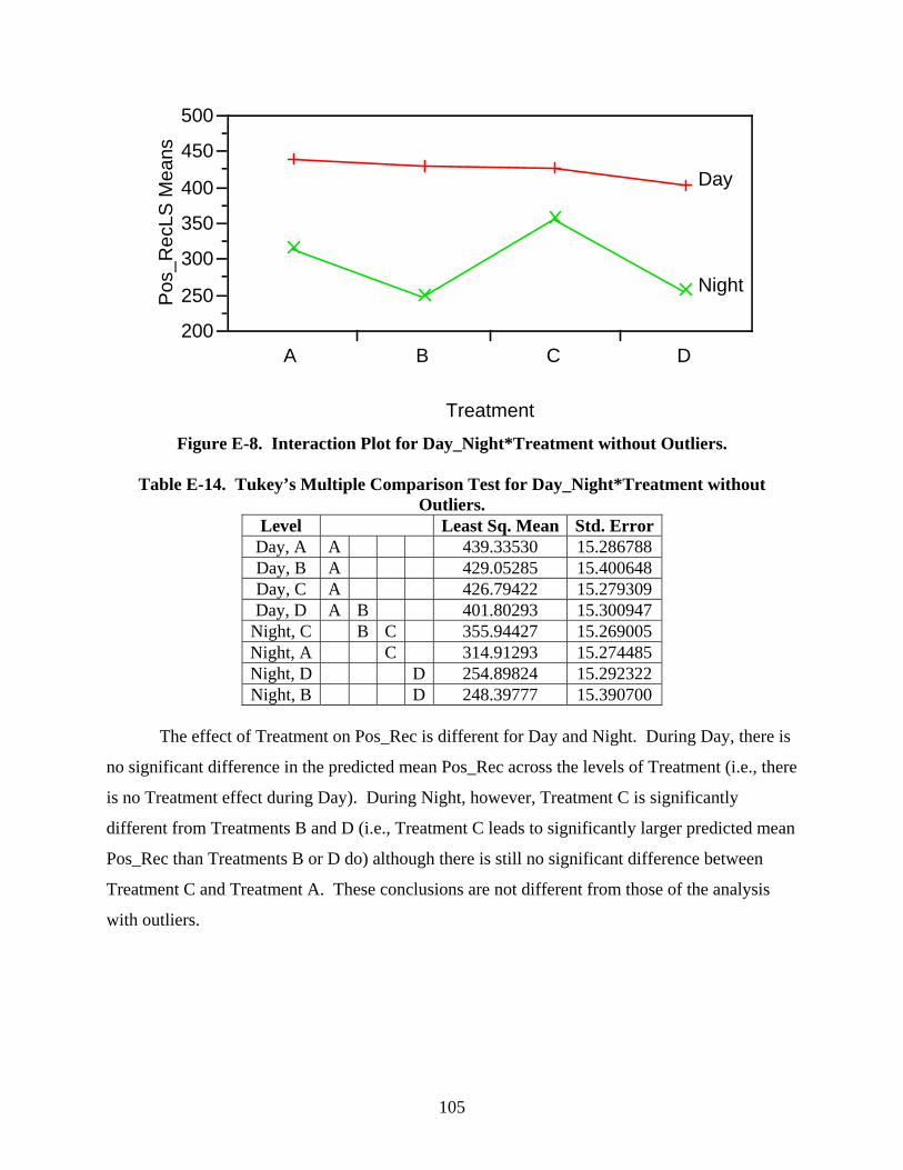
105

Figure E-8. Interaction Plot for Day_Night*Treatment without Outliers.

Table E-14. Tukey’s Multiple Comparison Test for Day_Night*Treatment without Outliers.

Level Least Sq. Mean Std. Error Day, A A 439.33530 15.286788 Day, B A 429.05285 15.400648 Day, C A 426.79422 15.279309 Day, D A B 401.80293 15.300947

Night, C B C 355.94427 15.269005 Night, A C 314.91293 15.274485 Night, D D 254.89824 15.292322 Night, B D 248.39777 15.390700





Pos_Rec than Treatments B or D do) although there is still no significant difference between

Treatment C and Treatment A. These conclusions are not different from those of the analysis

with outliers.

Pos

_Rec

LS M

eans

200

250

300

350

400

450

500

Day

Night

A B C D

Treatment

106

Figure E-9. Interaction Plot for Treatment*TargetLine without Outliers.

Table E-15. Tukey’s Multiple Comparison Test for Treatment*TargetLine without Outliers.

Level Least Sq. Mean Std. Error C, Top A 443.92480 18.798137

C, Middle A B 397.55443 13.662150 A, Bottom A B C 381.38235 18.926807

A, Top B C 377.03203 13.669108 B, Top A B C D 376.55373 19.431753

A, Middle A B C D 372.95796 18.803195 D, Middle B C D E 355.59670 18.798193

D, Top B C D 353.74485 13.662227 B, Bottom C D 342.18147 13.692646 C, Bottom C D E 332.62850 18.798137 B, Middle D E 297.44073 18.820313 D, Bottom E 275.71020 18.974154

The effect of TargetLine is different for each level of Treatment. For Treatment A or

Treatment B, the predicted mean Pos_Rec does not change significantly across the levels of

TargetLine (i.e., no significant effect of TargetLine is observed for Treatment A or Treatment B).

For Treatments C or D, however, there is a statistically significant effect of TargetLine on

predicted mean Pos_Rec. For Treatment C, Top TargetLine and Middle TargetLine lead to

higher predicted mean Pos_Rec than Bottom TargetLine does. For Treatment D, Top TargetLine

leads to higher predicted mean Pos_Rec than Bottom TargetLine does. Note also that

Treatment C has a higher least squares mean Pos_Rec than Treatment B does at TargetLine Top

though the difference is not statistically significant. The pattern of interaction plot of

Pos

_Rec

LS M

eans

200

250

300

350

400

450

500

AB

C

D

Bottom Middle Top

TargetLine

107

Treatment*TargetLine without outliers is now more consistent with that of the analysis of

Rec_Dist data.

Because the interaction effects Age Group*Treatment, Gender*Treatment, and


effects of Age Group, Gender, and/or Visual Acuity on Pos_Rec can be assessed. It can be

concluded based on the p-values for Age Group, Gender, and Visual Acuity Group that Age

Group and Visual Acuity have statistically significant effects on Pos_Rec at the significance

level α=0.05 while the effect of Gender is not statistically significant.

Table E-16 contains the analysis output without the five outliers, obtained by the

restricted maximum likelihood method under Model B implemented in JMP.

Table E-16. JMP Output for Rec_Dist under Model B without Outliers. Response Pos_Rec Summary of Fit RSquare 0.677209 RSquare Adj 0.631653 Root Mean Square Error 71.51173 Mean of Response 371.7007 Observations (or Sum Weights) 284

Effect Tests


Age Group 1 1 13 16691.33 3.2639 0.0940 Gender 1 1 13 63.07 0.0123 0.9133 Visual Acuity Group 1 1 13 8442.65 1.6509 0.2213 Day_Night 1 1 235 580625.87 113.5381 <0.0001 Treatment 3 3 235 144744.77 9.4347 <0.0001 TargetLine 2 2 235 101575.53 9.9313 <0.0001 Age Group*Treatment 3 3 235 12249.08 0.7984 0.4958 Gender*Treatment 3 3 235 11927.48 0.7775 0.5076 Day_Night*Treatment 3 3 235 88563.54 5.7727 0.0008 Treatment*TargetLine 6 6 235 108966.82 3.5513 0.0022 Visual Acuity Group*Treatment 3 3 235 11728.53 0.7645 0.5150 Contrast Sensitivity Group 2 2 13 6580.01 0.6433 0.5415 Contrast Sensitivity Group*Treatment 6 6 235 19952.27 0.6503 0.6899

Driver[Age Group, Gender, Visual Acuity Group, Contrast Sensitivity Group]&Random

19 13 235 369863.74 . .


Note again that the R-square value increased significantly compared to the analysis with

outliers. It can be observed from the Effect Tests table that the interaction effects between

108

Treatment and Day_Night and between Treatment and TargetLine are statistically significant at

α=0.05. Recall that the interaction effect between Treatment and Day_Night on Pos_Rec was

not significant in the previous analysis with outliers. Figure E-10 and Table E-17 contain the

interaction plot for Treatment*Day_Night and the corresponding multiple comparison test

results, respectively.

Figure E-10. Interaction Plot for Day_Night*Treatment without Outliers.

Table E-17. Tukey’s Multiple Comparison Test for Day_Night*Treatment. Level Least Sq. Mean Std. Error

Day, A A 450.77078 21.840717 Day, C A B 425.85524 21.736311 Day, B A B 423.46491 21.986933 Day, D A B 407.46147 21.736311

Night, C B C 373.81571 21.701533 Night, A C D 325.47781 21.792990 Night, D D E 259.86060 21.701533 Night, B E 234.65394 21.964303




different from Treatment B and D (i.e., Treatment C leads to significantly larger predicted mean

Pos_Rec than Treatment B or D does) although there is still no significant difference between

Pos

_Rec

LS M

eans

200

250

300

350

400

450

500

Day

Night

A B C D

Treatment

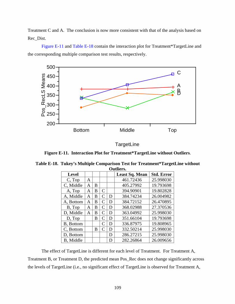
109

Treatment C and A. The conclusion is now more consistent with that of the analysis based on

Rec_Dist.

Figure E-11 and Table E-18 contain the interaction plot for Treatment*TargetLine and

the corresponding multiple comparison test results, respectively.

Figure E-11. Interaction Plot for Treatment*TargetLine without Outliers.

Table E-18. Tukey’s Multiple Comparison Test for Treatment*TargetLine without Outliers.

Level Least Sq. Mean Std. Error C, Top A 461.72436 25.998030

C, Middle A B 405.27992 19.793698 A, Top A B C 394.90901 19.802828

A, Middle A B C D 384.74234 26.004982 A, Bottom A B C D 384.72152 26.470895

B, Top A B C D 368.02988 27.370536 D, Middle A B C D 363.04992 25.998030

D, Top B C D 351.66104 19.793698 B, Bottom C D 336.87975 19.808965 C, Bottom B C D 332.50214 25.998030 D, Bottom D 286.27215 25.998030 B, Middle D 282.26864 26.009656

The effect of TargetLine is different for each level of Treatment. For Treatment A,

Treatment B, or Treatment D, the predicted mean Pos_Rec does not change significantly across

the levels of TargetLine (i.e., no significant effect of TargetLine is observed for Treatment A,

Pos

_Rec

LS M

eans

200

250

300

350

400

450

500

AB

C

D

Bottom Middle Top

TargetLine

110

Treatment B, or Treatment D). For Treatment C, however, Top TargetLine leads to significantly

higher predicted mean Pos_Rec than Bottom TargetLine does.

Note also that Treatments C and A have higher predicted mean Pos_Rec than

Treatment B does at TargetLine Top (though the difference is not statistically significant). The

pattern of interaction plot of Treatment*TargetLine without outliers is now more consistent with

that of the analysis of Rec_Dist data.


Treatment*Visual Acuity Group, and Treatment*Contrast Sensitivity Group in Table E-16 are

not statistically significant, the individual effects of Age Group, Gender, Visual Acuity Group,

and Contrast Sensitivity Group on Pos_Rec can be assessed. It can be concluded based on the p-

values for Age Group, Gender, Acuity Group, and Contrast Sensitivity Group that none of Age

Group, Gender, Visual Acuity Group, and Contrast Sensitivity Group have statistically

significant effects on Pos_Rec at α=0.05.

ANALYSIS BASED ON LEGIBILITY TASK DATA

In this analysis, the dependent variable is the calculated adjusted legibility distance

(Adjusted Leg_Dist). A split-plot model using Gender and Age Group as whole-plot factors,

along with Drivers as a nested random effect (nested within Gender and Age Group) and

Day_Night, Treatment (Font), Color, NumLine, and Target Line as split-plot factors, is applied

to the dataset consisting of 2,138 measurements on Adjusted Leg_Dist. Neither Visual Acuity

Group nor Contrast Sensitivity Group is included in the analysis because inclusion of either

variable eliminates many observations (213 when including Visual Acuity Group and 853 when

including Contrast Sensitivity Group) from the dataset (due to missing values).

In addition to the main effects defined from the whole-plot factors and the split-plot

factors, the two-way interaction effects between Treatment and other factors are included in the

model. Not all the two-way interaction effects or higher-order interaction effects could be

included due to the lack of degrees of freedom (i.e., there are not enough observations to test all

of those effects).


method implemented in JMP.

111

Table E-19. JMP Output for Leg_Dist.

Response Pos_Rec Summary of Fit RSquare 0.63712 RSquare Adj 0.632128 Root Mean Square Error 54.41674 Mean of Response 361.6791 Observations (or Sum Weights) 2138

Effect Tests


Age_Group 1 1 27 34499.0 11.6504 0.0020 Gender 1 1 27 5616.5 1.8967 0.1798 Day_Night 1 1 2081 4177082.7 1410.614 <0.0001 Color 2 2 2081 188765.3 31.8733 <0.0001 Treatment 3 3 2081 130156.4 14.6514 <0.0001 NumLine 1 1 2081 30631.9 10.3445 0.0013 TargetLine 2 2 2081 4177.7 0.7054 0.4940 Age_Group*Treatment 3 3 2081 11821.9 1.3308 0.2626 Gender*Treatment 3 3 2081 7298.6 0.8216 0.4819 Day_Night*Treatment 3 3 2081 30735.7 3.4599 0.0158 Color*Treatment 6 6 2081 257098.0 14.4705 <0.0001 Treatment*NumLine 3 3 2081 50533.7 5.6885 0.0007 Driver[Age_Group,Gender]& Random 30 27 2081 3418465.6 . .


It can be observed from the Effect Tests table that there are significant interaction effects

Day_Night*Treatment, Color*Treatment, and Treatment*NumLine. These significant

interaction effects indicate that the effect of Treatment can only be assessed conditionally on

each level of the other factor, Day_Night, Color, or NumLine. Plots for the statistically

significant interaction effects are presented in Figure E-12 to Figure E-14. Tukey’s multiple

comparison test results are also provided in Table E-20 to Table E-22. The conclusions drawn

based on the interaction plots and the multiple comparison procedures are presented right after

the multiple comparison test tables.

112


Table E-20. Tukey’s Multiple Comparison Test for Day_Night*Treatment. Level Least Sq. Mean Std. Error Day, C A 381.87430 10.588417 Day, A A B 379.14569 12.788690 Day, B A B 364.12155 10.705792 Day, D B 347.42868 10.049672

Night, A C 284.20186 10.595113 Night, C C 272.41052 10.636958 Night, B C 267.12149 10.533446 Night, D C 263.98578 12.856467

The effect of Treatment on Adjusted Leg_Dist is slightly different for Day and Night.

During Night, there is no significant difference in the least squares mean Adjusted Leg_Dist

across the levels of Treatment (i.e., there is no Treatment effect during Night). During Day,

Treatment C leads to higher predicted mean Adjusted Leg_Dist than Treatment D does although

there is no significant difference among Treatments C, A, and B.

Adj

uste

d Le

g_D

istL

S M

eans

200

250

300

350

400

Day

Night

A B C D

Treatment

113

Figure E-13. Interaction Plot for Treatment*Color.

Table E-21. Tukey’s Multiple Comparison Test for Treatment*Color. Level Least Sq. Mean Std. Error

Yellow, A A 341.64677 10.316567 White, A A 341.12806 10.320559 Yellow, D A B 337.91457 10.887041 Orange, C A B 336.42063 10.116955 Yellow, C A B 335.31813 10.115158 Yellow, B B C 318.74972 10.131855 White, B B C 316.72086 10.139046

Orange, A C 312.24650 10.326744 Orange, B C D 311.39398 10.117857 White, C C D 309.68847 10.124774 White, D D 289.97417 10.843028 Orange, D D 289.23294 10.831837

The effect of Treatment is different for each color. For Yellow, Treatment A leads to

higher predicted mean Adjusted Leg_Dist than Treatment B although there is no statistically

significant difference between Treatment A and Treatment C or Treatment D. For Orange,

Treatment C leads to higher predicted mean Adjusted Leg_Dist than Treatment A, Treatment B,

or Treatment D does. For White, Treatment A leads to higher predicted mean Adjusted

Leg_Dist than Treatment B, Treatment C, or Treatment D does.

Adju

sted

Leg

_Dis

tLS

Mea

ns

200

250

300

350

400

Orange

White

Yellow

A B C D

Treatment

114

Figure E-14. Interaction Plot for Treatment*NumLine.

Table E-22. Tukey’s Multiple Comparison Test for Treatment*NumLine. Level Least Sq. Mean Std. Error A, 2 A 335.61588 10.554394 C, 2 A 335.45304 10.526909 B, 2 A 335.16461 10.525832 A, 3 A B 327.73167 9.961490 C, 3 A B C 318.83178 10.704039 D, 2 B C D 309.71195 10.542262 D, 3 C D 301.70251 10.649709 B, 3 D 296.07843 10.771618

The effect of NumLine is different for each level of Treatment. For Treatment B,

NumLine 2 leads to higher predicted mean Adjusted Leg_Dist than NumLine 3 does. For

Treatments A, C, and D, however, there is no significant effect of NumLine.

Because the interaction effects Age Group*Treatment and Gender*Treatment in

Table E-19 are not statistically significant, the individual effects of Age Group and Gender can

be assessed. Only Age Group has a statistically significant effect on Adjusted Leg_Dist at the

significance level α=0.05. The effect of Gender is not statistically significant. There is no

statistically significant effect of TargetLine either.

Adj

uste

d Le

g_D

istL

S M

eans

200

250

300

350

400

A

B

CD

2 3

NumLine

115

A new variable “Conflict” has been added to the analysis to see if there is an effect due to

the conflict of words on the sign. The level of Conflict is either Yes or No and is assigned

according to the following rule:

• Two-line signs with a descender for the top word and an ascender for the bottom

word have conflict (a YES). Two-line signs with an ascender/ascender or

descender/descender combination do not have any conflict (a NO).

• The three-line signs with a descender/neutral/ascender word combination do not have

any conflict (a NO). The three-line signs with a descender/both/ascender word

combination do exhibit conflict. The middle word in this case has both ascender and

descender letters (a YES).

Table E-23 contains the analysis output under the model with an additional variable,

Conflict, obtained by the RML method implemented in JMP.

116

Table E-23. JMP Output for Adjusted Leg_Dist. Response Adjusted Leg_Dist Summary of Fit RSquare 0.640589 RSquare Adj 0.632128 Root Mean Square Error 54.41674 Mean of Response 361.6791 Observations (or Sum Weights) 2138

Effect Tests


Age_Group 1 1 27 34108.1 11.6241 0.0021 Gender 1 1 27 5574.1 1.8996 0.1794 Day_Night 1 1 2080 4185713.0 1426.492 <0.0001 Color 2 2 2080 226641.7 38.6198 <0.0001 Treatment 3 3 2080 175056.5 19.8864 <0.0001 NumLine 1 1 2080 14223.7 4.8474 0.0278 TargetLine 2 2 2080 4034.1 0.6874 0.5030 Age_Group*Treatment 3 3 2080 11740.5 1.3337 0.2617 Gender*Treatment 3 3 2080 7294.0 0.8286 0.4780 Day_Night*Treatment 3 3 2080 30754.6 3.4937 0.0151 Color*Treatment 6 6 2080 288634.1 16.3944 <0.0001 Treatment*NumLine 3 3 2080 42597.3 4.8391 0.0023 Conflict 1 1 2080 58900.6 20.0734 <0.0001 Driver[Age_Group,Gender] & Random 30 27 2080 3420781.7 . .


Table E-23 shows that there are no significant changes in conclusions for the effects of

interactions and the main effects from those of Table E-19, except the effect of Conflict has also

turned out to be statistically significant. The patterns of interaction plots, which are not

presented here due to limited space, are similar to those of Figure E-12 to Figure E-14.

Table E-24 and Figure E-15 contain the least squares means table and the least squares means

plot for the Adjusted Leg_Dist for each level of Conflict, respectively. Surprisingly, the effect of

Conflict turned out to be counter-intuitive. When there is a conflict (YES), the least squares

mean Adjusted Leg_Dist is higher than when there is no conflict although the difference does not

seem to be practically significant. The same can be said even in terms of the raw cell means (see

the last column of Table E-24).

117

Table E-24. Least Squares Means Table for Conflict. Level Least Sq. Mean Std. Error Mean

No 315.43176 9.3750888 334.578Yes 330.31132 9.5966543 340.862

Figure E-15. Least Squares Means Plot for Conflict.

Adj

uste

d Le

g_D

istL

S M

eans

200

250

300

350

400

No Yes

Conflict

118

DISTRIBUTIONS OF WHOLE-PLOT FACTORS

1416

F M

Figure E-16. Gender.

7

23

Old Young

Figure E-17. Age Group.

56

1

12

21

13 15 18 20 25 27

Figure E-18. Visual Acuity.

1 1 1 1

2

3

1 1 1 1 1 1

2

1 1 1

31 37 41 42 43 44 45 48 50 51 52 53 57 58 60 64

Figure E-19. Contrast Sensitivity.

Documents

Evaluation of the Clearview Font for Negative Contrast … · EVALUATION OF THE CLEARVIEW FONT FOR NEGATIVE CONTRAST TRAFFIC SIGNS 6. Performing Organization Code 7. ... longer legibility