Evaluation of the nitrogen sufficiency index for usewith high resolution, broadband aerial imageryin a commercial potato field

Tyler J. Nigon • David J. Mulla • Carl J. Rosen • Yafit Cohen •

Victor Alchanatis • Ronit Rud

Published online: 1 November 2013� Springer Science+Business Media New York 2013

Abstract The nitrogen sufficiency index (NSI) can be used for in-season variable rate

management of nitrogen (N) fertilizer to maintain productivity of potato (Solanum tu-

berosum, L.) while reducing leaching losses. The objective of this study was to evaluate the

implications of using high spatial resolution broad-band imagery for determining N pre-

scriptions at different growth stages. Aerial images were obtained for research plots, as

well as for a commercial potato field (59 ha) near Becker, Minnesota on 30, 56 and

79 days after emergence (DAE) with a Redlake MS4100 multispectral camera. In research

plots, experimental treatments included five N treatments with varying rates and timing of

N fertilizer, and two potato varieties, Russet Burbank and Alpine Russet. Spectral indices

investigated in this study adequately predicted N stress based on leaf N concentration (r2

values within dates ranged from 0.49 to 0.82). On 56 and 79 DAE, the Green Ratio

Vegetation Index (GRVI) normalized by an NSI that used the recommended rate and

timing from the research plots as a reference showed that most areas of the commercial

field did not require supplemental N fertilizer (using an NSI over-sufficiency threshold of

120 %). Based on regional guidelines, N was over-applied to the commercial field, but

in situations where N is applied more sparingly, a GRVI NSI threshold of 80 % should be

used to identify areas that are most suitable for supplemental N fertilizer. A practical

approach and the implications associated with using spectral data for in-season N man-

agement are proposed.

Keywords High spatial resolution imagery � Spectral indices � Chlorophyll

meter � Virtual reference � Coefficient of variation

T. J. Nigon (&) � D. J. Mulla � C. J. RosenDepartment of Soil, Water and Climate, University of Minnesota, Saint Paul, MN, USAe-mail: nigo0024@umn.edu

Y. Cohen � V. Alchanatis � R. RudAgricultural Research Organization, Volcani Center, Institute of Agricultural Engineering,Bet-Dagan, Israel

123

Precision Agric (2014) 15:202–226DOI 10.1007/s11119-013-9333-6

Introduction

The coarse textured soils typically used for irrigated potato (Solanum tuberosum, L.)

production are relatively low in organic matter and cation exchange capacity, and there-

fore, are generally low in soil nutrient reserves. The low inherent fertility of these soils,

coupled with the large nitrogen (N) requirement for a potato crop, leads to high fertilizer

inputs (Dean 1994). Potato plants are relatively shallow rooted compared to other field and

vegetable crops and are very sensitive to water stress (Bailey 2000; Lesczynski and Tanner

1976). This leads to below average nutrient uptake and poor nitrogen use efficiency (NUE),

which potentially results in high rates of nitrate leaching (Lynch et al. 2012; Rosen and

Bierman 2008; Zvomuya et al. 2003). Because of the health risks associated with nitrate-

contaminated groundwater (EPA 2009), it is becoming increasingly important to improve

N fertilizer management and reduce nitrate—N losses to groundwater. Previous studies

have shown that only about a third to a half of applied N is recovered by an irrigated potato

crop in years of moderate to heavy leaching (Errebhi et al. 1998; Waddell et al. 2000).

Therefore, precise spatial and temporal N management for irrigated potato is important to

optimize production and to minimize environmental N losses.

Matching the timing and rate of N fertilizer with the N needs of the crop during different

growth stages will help to optimize crop uptake while minimizing N losses (Canter 1997;

Errebhi et al. 1998). Increased NUE, N uptake and yields have been shown to result from

split applications of N fertilizer during tuber initiation and bulking, especially during

leaching years (Errebhi et al. 1998; Westermann et al. 1988; Nigon 2012b). The use of

fertigation provides a convenient method to split apply post-emergence N applications. The

challenge lies in the ability of the producer to estimate the appropriate rates and timing of

split N applications so that fertilizer N best matches crop demands. A logical strategy for

determining the exact rate and timing of post-emergence N applications is to make

adjustments based on in-season plant monitoring. Since this approach uses plant mea-

surements during the growing season, it is able to account for the effect of seasonal

weather conditions on crop N availability (Meisinger et al. 2008).

The opportunity exists to use aerial or satellite imagery to predict both spatial and

temporal variability in crop biophysical parameters that depend on crop N uptake such as

tissue N concentration and/or leaf chlorophyll concentration. Since plant N status is closely

related to chlorophyll in plant cell metabolism, spectral imagery can be used to monitor

crop N status because the spectral characteristics of green-leaved vegetation change as leaf

chlorophyll content changes (Stroppiana et al. 2012). There are a variety of multispectral

and hyperspectral cameras on the market that can be used to obtain canopy-level spectral

imagery. The spatial resolution capabilities of these cameras can range from a few cm to

tens of m, and this affects the ability of the camera to detect differences in reflectance of

spectral imagery. More specifically, the spectral variance detected by imagery can be

improved or compromised depending on its spatial resolution. It is characteristic for the

spectral variance of an image to be low at spatial resolutions of a few cm, and then reach a

peak at a resolution just smaller than the size of the objects in the image, followed by an

exponential decrease in local variance as the spatial resolution increases to the m scale

(Woodcock and Strahler 1987).

The nitrogen sufficiency index (NSI) can be applied to spectral imagery to normalize

the measurements to a non-limiting N reference area so that the ability of a producer to

make N management decisions can be enhanced (Peterson et al. 1993). Nitrogen suf-

ficiency indices based on spectral images can be implemented across a very large

spatial scale, and therefore, can be a very practical diagnostic tool for prescribing split

Precision Agric (2014) 15:202–226 203

123

applications of post-emergence N fertilizer (Tremblay et al. 2011). An NSI depends on

the use of a reference value, which has traditionally been a measurement from an over-

fertilized, N-rich area of the field (Blackmer and Schepers 1995; Denuit et al. 2002;

Sripada et al. 2008). Normalizing data to these over-fertilized, N-rich areas of the field

eliminates the need to develop a specific calibration function for each set of variables

or local conditions (e.g. soil type, variety, etc.; Shapiro et al. 2006). Over-fertilized

reference plots may not be suitable for determining supplemental N in a potato crop

because previous research has shown that spectral measurements for plots with medium

N rates have not been significantly different from spectral measurements for over-

fertilized plots (Denuit et al. 2002; Olivier et al. 2006). Furthermore, over-fertilization

of irrigated potato results in reduced tuber yields (Rosen and Bierman 2008). Over-

fertilized reference plots may not be sufficient for determining supplemental N in a

potato crop because plots or fields without N fertilizer are also needed to show that

chlorophyll meter readings are significantly different between the over-fertilized and

under-fertilized plots.

Research investigating the use of aerial-based broad-band spectral indices after being

normalized by an NSI has not been published for potato. Broad-band spectral data from

aerial imagery is able to account for within-field spatial variation, and therefore, can be a

more practical approach than chlorophyll meter readings for determining in-season N

prescriptions. The objectives of this study were: (i) to verify that spectral measurements

can indeed be a good indicator of N status in a potato crop, (ii) to determine how NSI

values can vary at different growth stages because of differences in the NSI reference used,

(iii) to identify whether estimates of N stress can be made in a commercial field without

using a reference N strip and (iv) to investigate how the spectral variance of imagery

representing attributes of a commercial potato field changes with spatial resolution at

different growth stages.

Materials and methods

Study sites

Field experiments were conducted in 2011 at the University of Minnesota Sand Plain

Research Farm (45�230N, 95�530W) near Becker, MN. In addition to data collected from

experimental plots, image data and plant samples were acquired for a 59 ha center-pivot

irrigated commercial field, which was located 3.2 km southeast of the experimental plots.

The northern *60 % of the commercial plot was planted into the Alpine Russet variety,

and the southern *40 % was planted into the Russet Burbank variety. There is approxi-

mately a 2.5-m change in elevation from the highest point of the commercial field

(northeast corner) to the lowest point (southeast corner); this equates to an average slope

less than 0.5 %. The soils at both locations are predominantly classified as an excessively

drained Hubbard–Mosford complex (sandy, mixed, frigid Typic Hapludolls). In the upper

30 cm of the soil profile, the textures of the Hubbard and the Mosford series are loamy

sand and sandy loam, respectively. In the upper 150 cm of soil, the available water holding

capacities of the Hubbard and the Mosford series are 10 and 12 cm, respectively. During

the growing season (April–September), the 30-year average temperature and rainfall

(1971–2000) are 16.5 �C and 550 mm, respectively (Midwest Regional Climate Center

2012).

204 Precision Agric (2014) 15:202–226

123

Experimental design of research plots

The field study at the research farm was set up as a randomized complete block design with

a split–split plot restriction on randomization replicated four times. The whole plot

treatment was irrigation rate (i.e., unstressed and stressed) to evaluate hypotheses about

interactions between water stress and N stress. Since climatic conditions during the study

were relatively wet, no water stress was observed, therefore only data from the unstressed

lots were used in this paper. Therefore, the data from the field study were analyzed using a

randomized complete block design with a split plot restriction on randomization. Irrigation

was applied with an overhead sprinkler system, and a water balance method was used to

schedule irrigation applications (Wright 2002). Timing of irrigation was variable between

years and depended on weather conditions. On average, approximately 4 days elapsed

between irrigation applications. From planting to harvest, cumulative rainfall was 57 cm

and cumulative irrigation was 26 cm. The subplot treatments included a low, medium and

high N rate with variable timing of post-emergence N applications for the high rate, for a

total of five N treatments. The N treatments were (in kg N ha-1): 34 early, 180 split, 270

split, 270 split ? surfactant (s) and 270 early (Table 1). On average, about two weeks

passed between split applications of post-emergence N for treatments 180 split, 270 split

and 270 split ? s. Treatments 270 split and 270 split ? s had the same rate and timing of

N application, but a soil surfactant (IrrigAid Gold, Paulsboro, NJ, USA) was applied to 270

split ? s at a rate of 10 L ha-1 to investigate the effects of the surfactant on soil moisture

and N uptake under different irrigation regimes; although determining the effects of the

soil surfactant was not an objective of this part of study, data from the 270 split ? s N

treatment were included in the dataset since the soil surfactant had little or no statistical

significance on the parameters measured. For the treatments that had split applications of

post-emergence N, actual N applied at the time of data acquisition varied (Table 2). The

planting and emergence N source was mono-ammonium phosphate and urea, respectively.

Post-emergence N was split applied five times by spray boom and tractor as 28 % urea-

ammonium nitrate solution. All post-emergence N was irrigated in immediately following

application.

The sub-subplot treatment consisted of two potato varieties (i.e., Russet Burbank and

Alpine Russet). Russet Burbank (RB), the most widely grown processing potato variety in

the U.S. and in Minnesota, has a mid-season maturity class of 111–120 days after planting

(Whitworth et al. 2011). Alpine Russet (AR) has a late-season maturity class of

121–130 days after planting, and is a relatively new variety grown in Minnesota. Com-

pared to RB, it has similar yields, superior processing quality after long-term storage and

greater resistance to water-stress induced tuber defects (Whitworth et al. 2011).

Whole ‘‘B’’ seed and cut ‘‘A’’ seed were used for the RB and AR varieties, respectively.

Seed was hand planted in furrows with 90-cm row spacing and approximately 30-cm

spacing between seed pieces within rows. Each plot consisted of seven 13.7 m rows. The

planting date was 29 April 2011, and plant emergence occurred on 24 May 2011. 2 days

after plant emergence in each year, emergence fertilizer was applied and rows were

mechanically hilled. Chemicals were applied as needed during the season for the control of

pests, disease and weeds according to standard practices in the region (Engel et al. 2012).

To estimate N supplied by precipitation and irrigation, water samples were collected

using a plastic bottle with a sealable cover; samples were frozen until analysis. The

concentrations of NO3–N and NH4–N from the samples were determined using a prototype

of a Wescan ammonia analyzer (Wescan instruments, Deerfield, IL, USA). Following

reduction of NO3–N to NH4–N using granular zinc, NO3–N was determined as the

Precision Agric (2014) 15:202–226 205

123

difference between NH4–N ? NO3–N and NH4–N (Carlson 1986; Carlson et al. 1990).

Total N supplied by rainfall ? irrigation throughout the growing season (from planting to

harvest) was 41 kg N ha-1.

Aerial image acquisition

Aerial multispectral imagery was acquired using the Airborne Environmental Research

Observational Camera (AEROCam, Grand Forks, ND, USA). The AEROCam was developed

and operated through a collaborative effort among the Upper Midwest Aerospace Consortium,

the School of Engineering & Mines and flight operations at the John D. Odegard School of

Aerospace Sciences at the University of North Dakota, Grand Forks, ND. The AEROCam uses

a Redlake MS4100 3-Charge Coupled Device (CCD) digital multispectral camera (Geospatial

Systems Incorporated, Rochester, NY, USA). The Redlake MS4100 uses three CCD imaging

sensors that feature a 1 920 9 1 080 pixel resolution with 8-bit quantization. The CCD sensors

captured energy at wavelengths ranging from 775–825 nm, 650–695 nm and 505–575 nm,

corresponding to broad-bands centered in the near-infrared (NIR), red and green regions of the

electromagnetic spectrum, respectively. The Redlake MS4100 was mounted on a Piper Arrow

PA28-201, and captured images of the treatment plots and commercial field at a 0.25-m spatial

resolution from approximately 235 m above the ground between 1 000 h and 1 500 h local

time on 23 June, 19 July and 11 August 2011; in the experimental year, these dates corresponded

to 30, 56 and 79 DAE, respectively (Table 2).

The AEROCam system includes an inertial measurement unit (IMU), GPS and specially

designed software application for image acquisition planning, processing and archiving

(Zhang et al. 2011). This allows for automatic geo-referencing and radiometric correction

of the acquired images. The AEROCam provided mosaicked multispectral images that

were radiometrically calibrated and geometrically rectified using the processes described

by Zhang et al. (2011). Image processing software (ENVI; version 4.8, Exelis, Inc.,

McLean, VA, USA) was used for all further image processing and analyses.

Plant sampling and field measurements

Leaf samples were collected on or within one day of each image date, as well as on 43 and

66 DAE (Table 2) at both the treatment plots and the commercial field. The fourth leaf

from the apex of the shoot was sampled on twenty plants in the fifth row from the alley in

Table 1 Nitrogen fertilizer application rates and timings for the research plots treatments

Nitrogen fertilizer treatment Timing of application Total N

Planting(kg N ha-1)

Emergence(kg N ha-1)

Post-emergence(kg N ha-1)

34 N (control) 34 0 0 34

180 N split 34 90 11.2 9 5a 180

270 N split 34 124 22.4 9 5a 270

270 N split ? surfactant (s) 34 124 22.4 9 5a 270

270 N early 34 124 112 270

On average, about 2 weeks passed between split applications of post-emergence N for treatments 180 split,270 split and 270 split ? surfactant (s)a Split applications of post-emergence N fertilizer occurred at 16, 34, 44, 57 and 76 days after emergence

206 Precision Agric (2014) 15:202–226

123

each treatment plot, as well as from four areas of the commercial field. Relative chloro-

phyll (SPAD-502, Spectrum Technologies, Plainfield, IL, USA) was immediately mea-

sured at a central point on the terminal leaflet between the midrib and leaf margin. The

twenty measurements from each plot or location within the commercial field were aver-

aged to represent a single value and were recorded. Following chlorophyll readings, leaf

samples were oven-dried at 60 �C, weighed for dry matter yield and were then ground with

a Wiley mill to pass a 2-mm sieve. Total N concentration in ground leaf samples was

determined with a combustion analyzer (Elementar Vario EL III, Elementar Americas Inc.,

Mt. Laurel, NJ, USA) following the methods of Horneck and Miller (1997).

Although whole plant samples may have been a better indicator of crop N status than

leaf samples, destructive removal of whole plants from the experimental plots would have

greatly reduced the vegetative cover represented by the imagery after several sample dates.

It is impractical to take whole plant samples for biomass and N uptake measurements for

routine diagnostic purposes (Zebarth and Rosen 2007). Because leaf/petiole tissue samples

are used by potato growers as N sufficiency guidelines for fertilizer N rate and timing

(Zebarth and Rosen 2007), they are justified as a means of detecting N status in this study.

Tubers were mechanically harvested from the third and fourth rows from the alley on 22

September 2011 (i.e. 146 days after planting). Tubers were weighed on a fresh weight

basis without washing to determine total tuber yield. Because of its sandy nature, negli-

gible amounts of soil adhered to the tubers.

Leaf N concentration and yield data were analyzed using PROC MIXED (SAS Institute

2008) with N treatments and variety considered as fixed variables and replications con-

sidered as random variables. For the main effects and interactions of the fixed variables,

pairwise comparisons of the least square means were made using the lsmeans/pdiff option

of the MODEL statement (a = 0.05). The PDMIX800 macro (Saxton 1998) was used to

place treatment means into letter groupings based on the pairwise comparisons.

Image analysis

Spectral data were always kept in image format until it was necessary to perform statistical

procedures outside of ENVI.

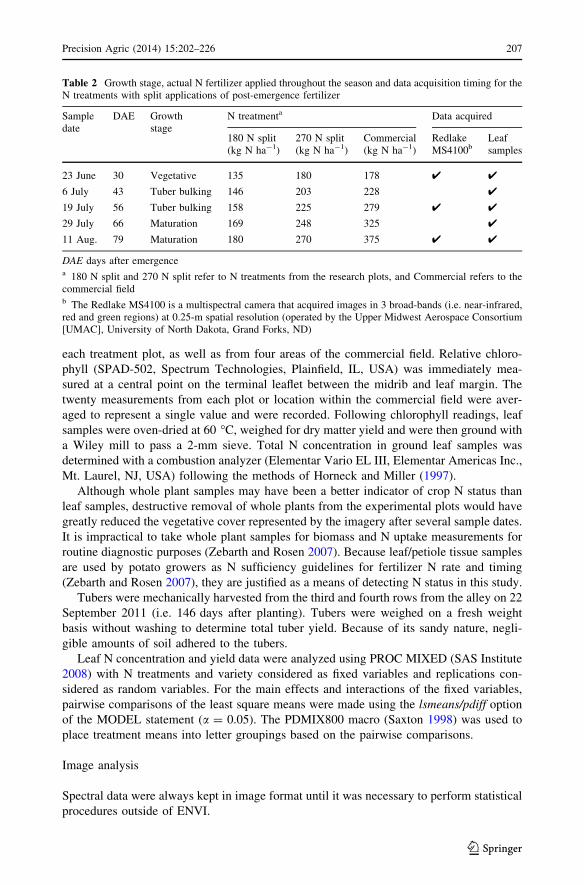
Table 2 Growth stage, actual N fertilizer applied throughout the season and data acquisition timing for theN treatments with split applications of post-emergence fertilizer

Sampledate

DAE Growthstage

N treatmenta Data acquired

180 N split(kg N ha-1)

270 N split(kg N ha-1)

Commercial(kg N ha-1)

RedlakeMS4100b

Leafsamples

23 June 30 Vegetative 135 180 178 4 4

6 July 43 Tuber bulking 146 203 228 4

19 July 56 Tuber bulking 158 225 279 4 4

29 July 66 Maturation 169 248 325 4

11 Aug. 79 Maturation 180 270 375 4 4

DAE days after emergencea 180 N split and 270 N split refer to N treatments from the research plots, and Commercial refers to thecommercial fieldb The Redlake MS4100 is a multispectral camera that acquired images in 3 broad-bands (i.e. near-infrared,red and green regions) at 0.25-m spatial resolution (operated by the Upper Midwest Aerospace Consortium[UMAC], University of North Dakota, Grand Forks, ND)

Precision Agric (2014) 15:202–226 207

123

Spectral indices

A preliminary analysis was conducted on images from the research plots using several

previously developed broad-band spectral indices to determine the indices that had the best

overall ability to detect N stress (Nigon 2012a). The correlation coefficient (r) was cal-

culated for each of these indices using the CORR procedure of SAS (SAS Institute 2008) to

determine the indices that had the best relationships with leaf N concentration on each date.

To determine which indices performed best overall, r2 was averaged for each index among

the four dates. Some of the indices that had the highest average r2 from this preliminary

analysis are listed in Table 3, and were used for comparison in all subsequent analyses in

this study. Broad-band normalized difference vegetation index (NDVI) did not perform

particularly well in the preliminary analysis, but it was included for comparison with other

indices and previously published research (Hansen and Schjoerring 2003; Jain et al. 2007;

Miao et al. 2009).

Indices that are able to integrate the effect of bare soil on reflectance were included in

the preliminary analysis, but were not included in the results/discussion of this study

because other indices were able to predict leaf N concentration better. Soil adjusted indices

included in the preliminary analysis included: SAVI (soil adjusted vegetation index; Huete

1988), MSAVI (modified soil adjusted vegetation index; Qi et al. 1994) and OSAVI

(optimized soil adjusted vegetation index; Rondeaux et al. 1996).

Pixel extraction

To extract pixel data for subsequent analysis, regions of interest (ROIs) were created for

images of each treatment plot at the research farm and for each variety at the commercial

field. Depending on the analysis, different pixels were used within each treatment plot or

field area. The treatment plot images were used for the prediction analysis; ROIs were

created to only include pixels representing the middle of the plots. The commercial field

images were used for the normalized N sufficiency and variability analyses. For the nor-

malized N sufficiency analysis, pixels that were most influenced by the effects of bare soil

were excluded from being used in data analysis; this was done by including pixels in the

ROIs only if they were above a minimum threshold when tested against a structural index

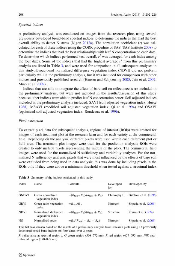
Table 3 Summary of the indices evaluated in this study

Index Name Formula Developedfor

Developed by

GNDVI Green normalizedvegetation index

=(RNIR-RG)/(RNIR ? RG) Chlorophyll Gitelson et al. (1996)

GRVI Green ratio vegetationindex

=RNIR/RG Nitrogen Sripada et al. (2006)

NDVI Normalized differencevegetation index

=(RNIR-RR)/(RNIR ? RR) Structure Rouse et al. (1974)

NG Normalized green =RG/(RNIR ? RR ? RG) Nitrogen Sripada et al. (2006)

This list was chosen based on the results of a preliminary analysis from research plots using 17 previouslydeveloped broad-band indices on four dates over 2 years

Ri reflectance at spectral region i, G green region (508–572 nm), R red region (657–695 nm), NIR near-infrared region (770–828 nm)

208 Precision Agric (2014) 15:202–226

123

(broad-band NDVI; Rouse et al. 1974). This technique effectively filtered out pixels that

were most influenced by bare soil so that only the pixels that represented a high proportion

of vegetation were used in the NSI analysis. For the variability analysis, all the pixels

within the commercial field were used.

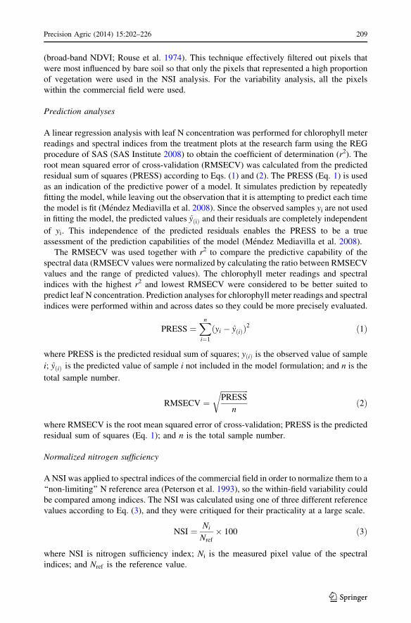
Prediction analyses

A linear regression analysis with leaf N concentration was performed for chlorophyll meter

readings and spectral indices from the treatment plots at the research farm using the REG

procedure of SAS (SAS Institute 2008) to obtain the coefficient of determination (r2). The

root mean squared error of cross-validation (RMSECV) was calculated from the predicted

residual sum of squares (PRESS) according to Eqs. (1) and (2). The PRESS (Eq. 1) is used

as an indication of the predictive power of a model. It simulates prediction by repeatedly

fitting the model, while leaving out the observation that it is attempting to predict each time

the model is fit (Mendez Mediavilla et al. 2008). Since the observed samples yi are not used

in fitting the model, the predicted values y ið Þ and their residuals are completely independent

of yi. This independence of the predicted residuals enables the PRESS to be a true

assessment of the prediction capabilities of the model (Mendez Mediavilla et al. 2008).

The RMSECV was used together with r2 to compare the predictive capability of the

spectral data (RMSECV values were normalized by calculating the ratio between RMSECV

values and the range of predicted values). The chlorophyll meter readings and spectral

indices with the highest r2 and lowest RMSECV were considered to be better suited to

predict leaf N concentration. Prediction analyses for chlorophyll meter readings and spectral

indices were performed within and across dates so they could be more precisely evaluated.

PRESS ¼Xn

i¼1

ðyi � y ið ÞÞ2 ð1Þ

where PRESS is the predicted residual sum of squares; y ið Þ is the observed value of sample

i; yðiÞ is the predicted value of sample i not included in the model formulation; and n is the

total sample number.

RMSECV ¼ffiffiffiffiffiffiffiffiffiffiffiffiffiffiffiPRESS

n

rð2Þ

where RMSECV is the root mean squared error of cross-validation; PRESS is the predicted

residual sum of squares (Eq. 1); and n is the total sample number.

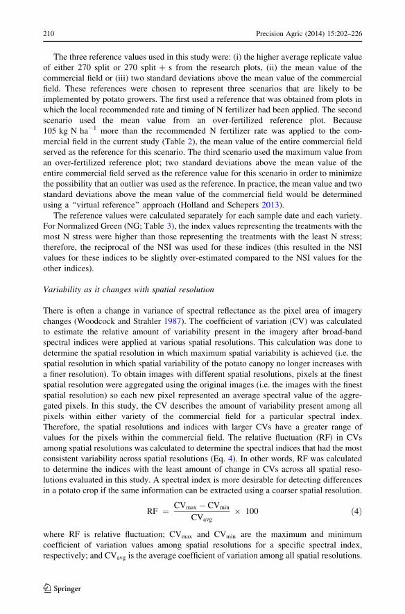
Normalized nitrogen sufficiency

A NSI was applied to spectral indices of the commercial field in order to normalize them to a

‘‘non-limiting’’ N reference area (Peterson et al. 1993), so the within-field variability could

be compared among indices. The NSI was calculated using one of three different reference

values according to Eq. (3), and they were critiqued for their practicality at a large scale.

NSI ¼ Ni

Nref

� 100 ð3Þ

where NSI is nitrogen sufficiency index; Ni is the measured pixel value of the spectral

indices; and Nref is the reference value.

Precision Agric (2014) 15:202–226 209

123

The three reference values used in this study were: (i) the higher average replicate value

of either 270 split or 270 split ? s from the research plots, (ii) the mean value of the

commercial field or (iii) two standard deviations above the mean value of the commercial

field. These references were chosen to represent three scenarios that are likely to be

implemented by potato growers. The first used a reference that was obtained from plots in

which the local recommended rate and timing of N fertilizer had been applied. The second

scenario used the mean value from an over-fertilized reference plot. Because

105 kg N ha-1 more than the recommended N fertilizer rate was applied to the com-

mercial field in the current study (Table 2), the mean value of the entire commercial field

served as the reference for this scenario. The third scenario used the maximum value from

an over-fertilized reference plot; two standard deviations above the mean value of the

entire commercial field served as the reference value for this scenario in order to minimize

the possibility that an outlier was used as the reference. In practice, the mean value and two

standard deviations above the mean value of the commercial field would be determined

using a ‘‘virtual reference’’ approach (Holland and Schepers 2013).

The reference values were calculated separately for each sample date and each variety.

For Normalized Green (NG; Table 3), the index values representing the treatments with the

most N stress were higher than those representing the treatments with the least N stress;

therefore, the reciprocal of the NSI was used for these indices (this resulted in the NSI

values for these indices to be slightly over-estimated compared to the NSI values for the

other indices).

Variability as it changes with spatial resolution

There is often a change in variance of spectral reflectance as the pixel area of imagery

changes (Woodcock and Strahler 1987). The coefficient of variation (CV) was calculated

to estimate the relative amount of variability present in the imagery after broad-band

spectral indices were applied at various spatial resolutions. This calculation was done to

determine the spatial resolution in which maximum spatial variability is achieved (i.e. the

spatial resolution in which spatial variability of the potato canopy no longer increases with

a finer resolution). To obtain images with different spatial resolutions, pixels at the finest

spatial resolution were aggregated using the original images (i.e. the images with the finest

spatial resolution) so each new pixel represented an average spectral value of the aggre-

gated pixels. In this study, the CV describes the amount of variability present among all

pixels within either variety of the commercial field for a particular spectral index.

Therefore, the spatial resolutions and indices with larger CVs have a greater range of

values for the pixels within the commercial field. The relative fluctuation (RF) in CVs

among spatial resolutions was calculated to determine the spectral indices that had the most

consistent variability across spatial resolutions (Eq. 4). In other words, RF was calculated

to determine the indices with the least amount of change in CVs across all spatial reso-

lutions evaluated in this study. A spectral index is more desirable for detecting differences

in a potato crop if the same information can be extracted using a coarser spatial resolution.

RF ¼ CVmax � CVmin

CVavg

� 100 ð4Þ

where RF is relative fluctuation; CVmax and CVmin are the maximum and minimum

coefficient of variation values among spatial resolutions for a specific spectral index,

respectively; and CVavg is the average coefficient of variation among all spatial resolutions.

210 Precision Agric (2014) 15:202–226

123

Results and discussion

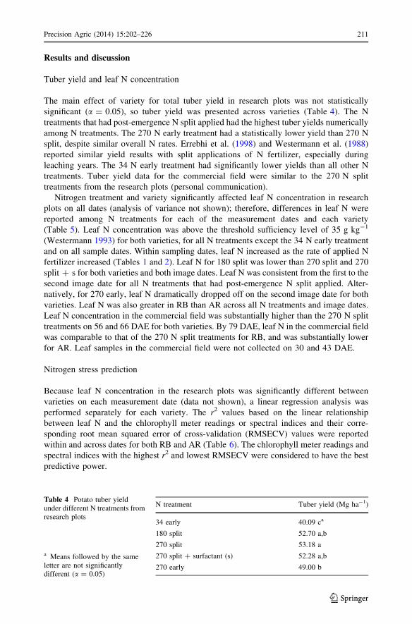
Tuber yield and leaf N concentration

The main effect of variety for total tuber yield in research plots was not statistically

significant (a = 0.05), so tuber yield was presented across varieties (Table 4). The N

treatments that had post-emergence N split applied had the highest tuber yields numerically

among N treatments. The 270 N early treatment had a statistically lower yield than 270 N

split, despite similar overall N rates. Errebhi et al. (1998) and Westermann et al. (1988)

reported similar yield results with split applications of N fertilizer, especially during

leaching years. The 34 N early treatment had significantly lower yields than all other N

treatments. Tuber yield data for the commercial field were similar to the 270 N split

treatments from the research plots (personal communication).

Nitrogen treatment and variety significantly affected leaf N concentration in research

plots on all dates (analysis of variance not shown); therefore, differences in leaf N were

reported among N treatments for each of the measurement dates and each variety

(Table 5). Leaf N concentration was above the threshold sufficiency level of 35 g kg-1

(Westermann 1993) for both varieties, for all N treatments except the 34 N early treatment

and on all sample dates. Within sampling dates, leaf N increased as the rate of applied N

fertilizer increased (Tables 1 and 2). Leaf N for 180 split was lower than 270 split and 270

split ? s for both varieties and both image dates. Leaf N was consistent from the first to the

second image date for all N treatments that had post-emergence N split applied. Alter-

natively, for 270 early, leaf N dramatically dropped off on the second image date for both

varieties. Leaf N was also greater in RB than AR across all N treatments and image dates.

Leaf N concentration in the commercial field was substantially higher than the 270 N split

treatments on 56 and 66 DAE for both varieties. By 79 DAE, leaf N in the commercial field

was comparable to that of the 270 N split treatments for RB, and was substantially lower

for AR. Leaf samples in the commercial field were not collected on 30 and 43 DAE.

Nitrogen stress prediction

Because leaf N concentration in the research plots was significantly different between

varieties on each measurement date (data not shown), a linear regression analysis was

performed separately for each variety. The r2 values based on the linear relationship

between leaf N and the chlorophyll meter readings or spectral indices and their corre-

sponding root mean squared error of cross-validation (RMSECV) values were reported

within and across dates for both RB and AR (Table 6). The chlorophyll meter readings and

spectral indices with the highest r2 and lowest RMSECV were considered to have the best

predictive power.

Table 4 Potato tuber yieldunder different N treatments fromresearch plots

a Means followed by the sameletter are not significantlydifferent (a = 0.05)

N treatment Tuber yield (Mg ha-1)

34 early 40.09 ca

180 split 52.70 a,b

270 split 53.18 a

270 split ? surfactant (s) 52.28 a,b

270 early 49.00 b

Precision Agric (2014) 15:202–226 211

123

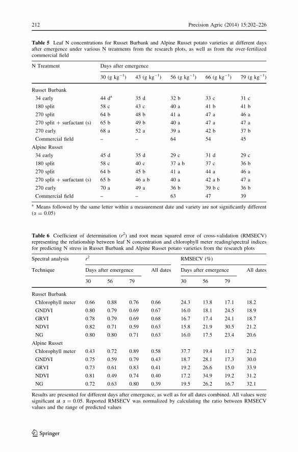
Table 5 Leaf N concentrations for Russet Burbank and Alpine Russet potato varieties at different daysafter emergence under various N treatments from the research plots, as well as from the over-fertilizedcommercial field

N Treatment Days after emergence

30 (g kg-1) 43 (g kg-1) 56 (g kg-1) 66 (g kg-1) 79 (g kg-1)

Russet Burbank

34 early 44 da 35 d 32 b 33 c 31 c

180 split 58 c 43 c 40 a 41 b 41 b

270 split 64 b 48 b 41 a 47 a 46 a

270 split ? surfactant (s) 65 b 49 b 40 a 47 a 47 a

270 early 68 a 52 a 39 a 42 b 37 b

Commercial field – – 64 54 45

Alpine Russet

34 early 45 d 35 d 29 c 31 d 29 c

180 split 58 c 40 c 37 a b 37 c 36 b

270 split 64 b 45 b 41 a 44 a 46 a

270 split ? surfactant (s) 65 b 46 a b 40 a 42 a b 47 a

270 early 70 a 49 a 36 b 39 b c 36 b

Commercial field – – 63 47 39

a Means followed by the same letter within a measurement date and variety are not significantly different(a = 0.05)

Table 6 Coefficient of determination (r2) and root mean squared error of cross-validation (RMSECV)representing the relationship between leaf N concentration and chlorophyll meter reading/spectral indicesfor predicting N stress in Russet Burbank and Alpine Russet potato varieties from the research plots

Spectral analysis r2 RMSECV (%)

Technique Days after emergence All dates Days after emergence All dates

30 56 79 30 56 79

Russet Burbank

Chlorophyll meter 0.66 0.88 0.76 0.66 24.3 13.8 17.1 18.2

GNDVI 0.80 0.79 0.69 0.67 16.0 18.1 24.5 18.9

GRVI 0.78 0.79 0.69 0.68 16.7 17.4 24.1 18.7

NDVI 0.82 0.71 0.59 0.63 15.8 21.9 30.5 21.2

NG 0.80 0.80 0.71 0.63 16.0 17.5 23.4 20.6

Alpine Russet

Chlorophyll meter 0.43 0.72 0.89 0.58 37.7 19.4 11.7 21.2

GNDVI 0.75 0.59 0.79 0.43 18.7 28.1 17.3 30.0

GRVI 0.73 0.61 0.83 0.41 19.2 26.6 15.0 33.9

NDVI 0.81 0.49 0.74 0.40 17.2 34.9 19.2 31.2

NG 0.72 0.63 0.80 0.39 19.5 26.2 16.7 32.1

Results are presented for different days after emergence, as well as for all dates combined. All values weresignificant at a = 0.05. Reported RMSECV was normalized by calculating the ratio between RMSECVvalues and the range of predicted values

212 Precision Agric (2014) 15:202–226

123

The indices that resulted in the highest r2 values and corresponding RMSECV varied by

date and variety (Table 6). The broad-band indices that could best predict leaf N concen-

tration in the research plots within dates (based on the frequency of highest r2 and lowest

RMSECV values) were NG for RB and GRVI for AR. GNDVI did have very similar r2 and

RMSECV values for both varieties, however. All broad-band indices performed better than

the chlorophyll meter readings on 30 DAE for both varieties; on each of the later dates, the

chlorophyll meter readings performed better than the broad-band indices.

Chlorophyll meter readings and spectral indices from the research plots were evaluated

over all dates to determine the measurement or index that could best predict N stress

regardless of growth stage. Over all dates, the r2 and RMSECV values for the chlorophyll

meter readings and the broad-band indices were significant; however, the chlorophyll

meter readings and spectral indices did not have as strong of a relationship with leaf N

concentration over all dates as they did within dates (r2 values ranged from 0.39 to 0.68

and RMSECV values ranged from 18 to 34 % over all dates). The GRVI was able to

predict N stress better than all other broad-band indices, and was able to predict N stress

better than the chlorophyll meter for the RB variety (Table 6).

Compared to the other indices, NDVI could predict leaf N concentration well on 30

DAE, but not on the other dates. This is because NDVI is a structural index that is most

sensitive to crop cover up to 90 % crop closures; after 90 % closure, NDVI values plateau

(Barnes et al. 2000), even when leaf N concentrations vary among N treatments. Therefore,

after canopy closure, NDVI does a poor job at detecting N stress, even though it is an

important stage to be able to distinguish between plants that may be under N stress. Since a

preliminary analysis was performed to select the best of several indices, the r2 values and

corresponding RMSECV for the reported indices were nearly similar (the range between

the best and worst indices on each date was always less than 0.14 and 9 % for r2 and

RMSECV, respectively). These N stress prediction analyses verify that broad-band spectral

indices have a good relationship with leaf N concentration, particularly within dates.

Feasibility of using a nitrogen sufficiency index

A well fertilized reference plot has worked well for NSI research in corn, but this may not be

the best approach in potatoes. Denuit et al. (2002) and Olivier et al. (2006) suggest that a lack

of significance between N treatments was the primary reason that using an over-fertilized

reference plot was not suitable to calculate NSIs for a potato crop. Contrary to their results,

chlorophyll meter readings for the high N rate in the current study were higher than chlo-

rophyll meter readings for the lower N rates. This was the case on all dates for the AR variety,

and all but the first date for the RB variety (data not shown). Because over-fertilization of N

can negatively affect tuber yield, it is plausible that spectral data representing a potato crop

canopy would also be affected by N over-fertilization. An NSI sufficiency threshold of 95 %

is used as a threshold to initiate fertilization in many studies across different crops, even

though it is somewhat arbitrary (Peterson et al. 1993; Varvel et al. 1997; Zebarth et al. 2002;

Holland and Schepers 2013). It is important to understand how the choice of a reference plot

can affect NSI values (and therefore, the optimum NSI sufficiency threshold) used to

determine the rate and timing of supplemental N fertilizer. Any variation in how an NSI

reference plot is managed can ultimately influence the conditions in which supplemental N

fertilizer would be applied. To determine differences among NSI references, three NSI

reference scenarios were compared by applying them to chlorophyll meter readings and four

broad-band indices from a commercial potato field (Tables 7 and 8).

Precision Agric (2014) 15:202–226 213

123

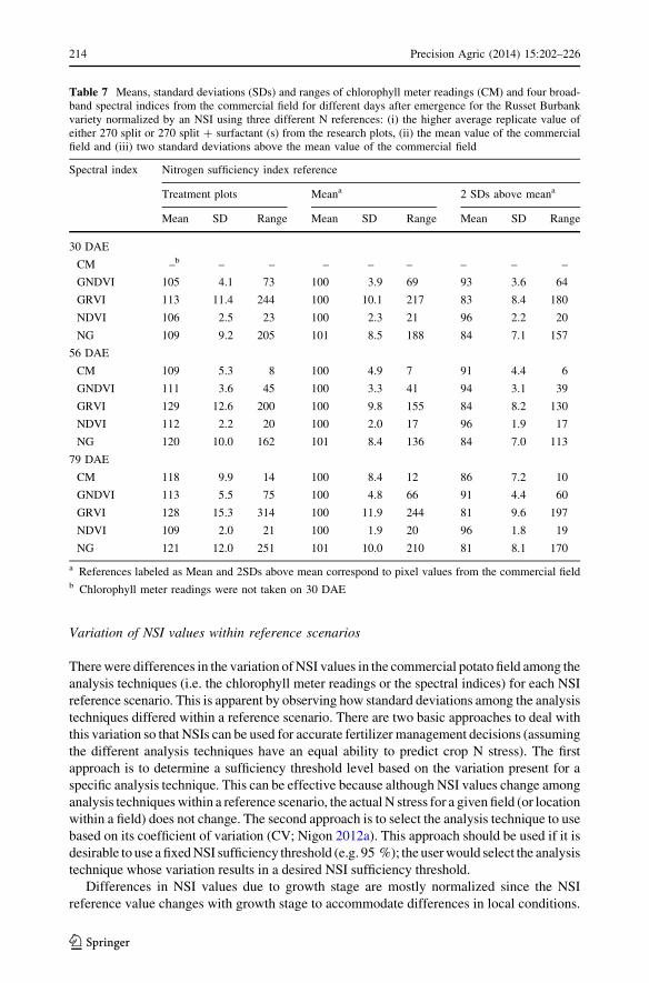
Variation of NSI values within reference scenarios

There were differences in the variation of NSI values in the commercial potato field among the

analysis techniques (i.e. the chlorophyll meter readings or the spectral indices) for each NSI

reference scenario. This is apparent by observing how standard deviations among the analysis

techniques differed within a reference scenario. There are two basic approaches to deal with

this variation so that NSIs can be used for accurate fertilizer management decisions (assuming

the different analysis techniques have an equal ability to predict crop N stress). The first

approach is to determine a sufficiency threshold level based on the variation present for a

specific analysis technique. This can be effective because although NSI values change among

analysis techniques within a reference scenario, the actual N stress for a given field (or location

within a field) does not change. The second approach is to select the analysis technique to use

based on its coefficient of variation (CV; Nigon 2012a). This approach should be used if it is

desirable to use a fixed NSI sufficiency threshold (e.g. 95 %); the user would select the analysis

technique whose variation results in a desired NSI sufficiency threshold.

Differences in NSI values due to growth stage are mostly normalized since the NSI

reference value changes with growth stage to accommodate differences in local conditions.

Table 7 Means, standard deviations (SDs) and ranges of chlorophyll meter readings (CM) and four broad-band spectral indices from the commercial field for different days after emergence for the Russet Burbankvariety normalized by an NSI using three different N references: (i) the higher average replicate value ofeither 270 split or 270 split ? surfactant (s) from the research plots, (ii) the mean value of the commercialfield and (iii) two standard deviations above the mean value of the commercial field

Spectral index Nitrogen sufficiency index reference

Treatment plots Meana 2 SDs above meana

Mean SD Range Mean SD Range Mean SD Range

30 DAE

CM –b – – – – – – – –

GNDVI 105 4.1 73 100 3.9 69 93 3.6 64

GRVI 113 11.4 244 100 10.1 217 83 8.4 180

NDVI 106 2.5 23 100 2.3 21 96 2.2 20

NG 109 9.2 205 101 8.5 188 84 7.1 157

56 DAE

CM 109 5.3 8 100 4.9 7 91 4.4 6

GNDVI 111 3.6 45 100 3.3 41 94 3.1 39

GRVI 129 12.6 200 100 9.8 155 84 8.2 130

NDVI 112 2.2 20 100 2.0 17 96 1.9 17

NG 120 10.0 162 101 8.4 136 84 7.0 113

79 DAE

CM 118 9.9 14 100 8.4 12 86 7.2 10

GNDVI 113 5.5 75 100 4.8 66 91 4.4 60

GRVI 128 15.3 314 100 11.9 244 81 9.6 197

NDVI 109 2.0 21 100 1.9 20 96 1.8 19

NG 121 12.0 251 101 10.0 210 81 8.1 170

a References labeled as Mean and 2SDs above mean correspond to pixel values from the commercial fieldb Chlorophyll meter readings were not taken on 30 DAE

214 Precision Agric (2014) 15:202–226

123

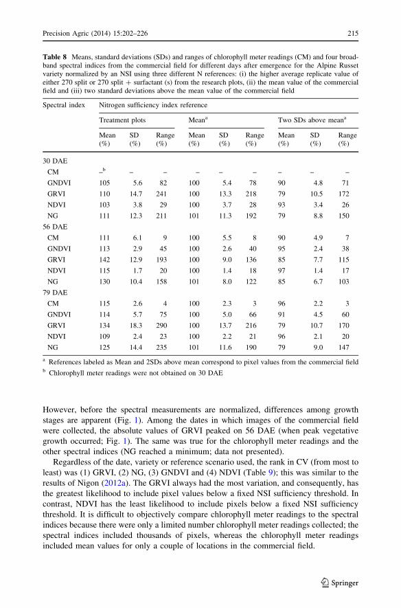
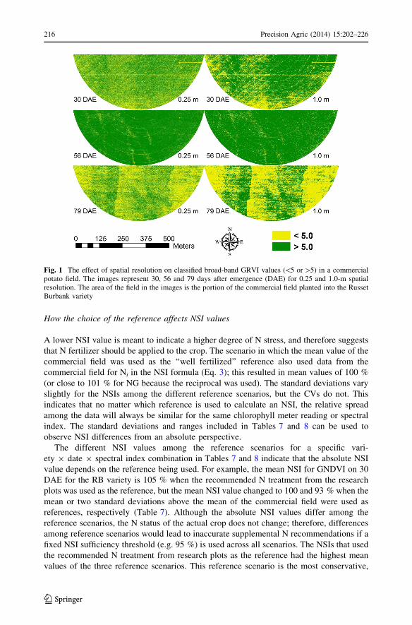
However, before the spectral measurements are normalized, differences among growth

stages are apparent (Fig. 1). Among the dates in which images of the commercial field

were collected, the absolute values of GRVI peaked on 56 DAE (when peak vegetative

growth occurred; Fig. 1). The same was true for the chlorophyll meter readings and the

other spectral indices (NG reached a minimum; data not presented).

Regardless of the date, variety or reference scenario used, the rank in CV (from most to

least) was (1) GRVI, (2) NG, (3) GNDVI and (4) NDVI (Table 9); this was similar to the

results of Nigon (2012a). The GRVI always had the most variation, and consequently, has

the greatest likelihood to include pixel values below a fixed NSI sufficiency threshold. In

contrast, NDVI has the least likelihood to include pixels below a fixed NSI sufficiency

threshold. It is difficult to objectively compare chlorophyll meter readings to the spectral

indices because there were only a limited number chlorophyll meter readings collected; the

spectral indices included thousands of pixels, whereas the chlorophyll meter readings

included mean values for only a couple of locations in the commercial field.

Table 8 Means, standard deviations (SDs) and ranges of chlorophyll meter readings (CM) and four broad-band spectral indices from the commercial field for different days after emergence for the Alpine Russetvariety normalized by an NSI using three different N references: (i) the higher average replicate value ofeither 270 split or 270 split ? surfactant (s) from the research plots, (ii) the mean value of the commercialfield and (iii) two standard deviations above the mean value of the commercial field

Spectral index Nitrogen sufficiency index reference

Treatment plots Meana Two SDs above meana

Mean(%)

SD(%)

Range(%)

Mean(%)

SD(%)

Range(%)

Mean(%)

SD(%)

Range(%)

30 DAE

CM –b – – – – – – – –

GNDVI 105 5.6 82 100 5.4 78 90 4.8 71

GRVI 110 14.7 241 100 13.3 218 79 10.5 172

NDVI 103 3.8 29 100 3.7 28 93 3.4 26

NG 111 12.3 211 101 11.3 192 79 8.8 150

56 DAE

CM 111 6.1 9 100 5.5 8 90 4.9 7

GNDVI 113 2.9 45 100 2.6 40 95 2.4 38

GRVI 142 12.9 193 100 9.0 136 85 7.7 115

NDVI 115 1.7 20 100 1.4 18 97 1.4 17

NG 130 10.4 158 101 8.0 122 85 6.7 103

79 DAE

CM 115 2.6 4 100 2.3 3 96 2.2 3

GNDVI 114 5.7 75 100 5.0 66 91 4.5 60

GRVI 134 18.3 290 100 13.7 216 79 10.7 170

NDVI 109 2.4 23 100 2.2 21 96 2.1 20

NG 125 14.4 235 101 11.6 190 79 9.0 147

a References labeled as Mean and 2SDs above mean correspond to pixel values from the commercial fieldb Chlorophyll meter readings were not obtained on 30 DAE

Precision Agric (2014) 15:202–226 215

123

How the choice of the reference affects NSI values

A lower NSI value is meant to indicate a higher degree of N stress, and therefore suggests

that N fertilizer should be applied to the crop. The scenario in which the mean value of the

commercial field was used as the ‘‘well fertilized’’ reference also used data from the

commercial field for Ni in the NSI formula (Eq. 3); this resulted in mean values of 100 %

(or close to 101 % for NG because the reciprocal was used). The standard deviations vary

slightly for the NSIs among the different reference scenarios, but the CVs do not. This

indicates that no matter which reference is used to calculate an NSI, the relative spread

among the data will always be similar for the same chlorophyll meter reading or spectral

index. The standard deviations and ranges included in Tables 7 and 8 can be used to

observe NSI differences from an absolute perspective.

The different NSI values among the reference scenarios for a specific vari-

ety 9 date 9 spectral index combination in Tables 7 and 8 indicate that the absolute NSI

value depends on the reference being used. For example, the mean NSI for GNDVI on 30

DAE for the RB variety is 105 % when the recommended N treatment from the research

plots was used as the reference, but the mean NSI value changed to 100 and 93 % when the

mean or two standard deviations above the mean of the commercial field were used as

references, respectively (Table 7). Although the absolute NSI values differ among the

reference scenarios, the N status of the actual crop does not change; therefore, differences

among reference scenarios would lead to inaccurate supplemental N recommendations if a

fixed NSI sufficiency threshold (e.g. 95 %) is used across all scenarios. The NSIs that used

the recommended N treatment from research plots as the reference had the highest mean

values of the three reference scenarios. This reference scenario is the most conservative,

Fig. 1 The effect of spatial resolution on classified broad-band GRVI values (\5 or [5) in a commercialpotato field. The images represent 30, 56 and 79 days after emergence (DAE) for 0.25 and 1.0-m spatialresolution. The area of the field in the images is the portion of the commercial field planted into the RussetBurbank variety

216 Precision Agric (2014) 15:202–226

123

and has the least likelihood of over-application of supplemental N fertilizer. In contrast, the

NSIs that used two standard deviations above the mean from the commercial field as the

reference had the lowest mean values (this scenario has the highest likelihood of over-

application of supplemental N fertilizer).

The commercial field had more applied N than the treatment plots with the recom-

mended rate on each date except 30 DAE (Table 2). Tuber yields for the commercial field

were slightly lower than that of the research plots for the 270 N split treatments (personal

communication). Observations of lower tuber yields for the over-fertilized commercial

field is consistent with previous research on irrigated potato in central Minnesota, showing

that over-fertilization with N reduces yield (Rosen and Bierman 2008). Research suggests

that tuber yield plateaus and actually declines for N fertilizer rates greater than

*270 kg ha-1 (Rosen and Bierman 2008). The commercial field also had higher leaf N

concentrations than the treatment plots with the recommended rate on 56 and 66 DAE

(Table 5). Although leaf samples were not collected on 30 or 43 DAE, it is likely that leaf

N concentration was also higher in the commercial field on 43 DAE. This implies that

over-fertilization in the commercial field resulted in increased leaf N concentrations and

decreased yield relative to adequately fertilized research plots.

For both varieties, all NSI values in the commercial field were above 100 % when the

recommended rate from research plots was used as a reference (Tables 7, 8). This demon-

strates that over-fertilization in the commercial field also resulted in increased NSI values for

all spectral analysis techniques. Leaf samples and spectral measurements from the research

plots were typically collected immediately prior to N fertilization, however, and there was

potentially a slight N stress present during the times of the measurements (Tables 1, 2).

Suppose we use 95 % as a fixed NSI sufficiency threshold to determine supplemental N

fertilizer applications. It is important to note that using a fixed NSI sufficiency threshold

among multiple spectral analysis techniques (chlorophyll meter readings or spectral

indices) that have different CVs will likely result in different N sufficiency results (Nigon

2012a). This could ultimately lead to conflicting N fertilizer recommendations for an

equivalent level of crop N stress among spectral analysis techniques. Because the mean

NSI values were all above 100 % when the recommended rate from research plots was

used as the reference (Tables 7, 8), most (or all) of the commercial field should not have

received additional N fertilizer. This depends on which spectral analysis technique is used;

techniques with low standard deviations and low CVs (e.g. GNDVI and NDVI) are the

least likely to show pixels to be below the 95 % NSI sufficiency threshold, and techniques

with higher standard deviations (e.g. chlorophyll meter readings, GRVI and NG) are most

likely to show pixels to be below the 95 % NSI sufficiency threshold. The NSI values of

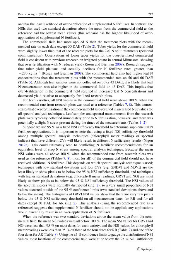
the spectral indices were normally distributed (Fig. 2), so a very small proportion of NSI

values occurred outside of the 95 % confidence limits (two standard deviations above and

below the mean). The histograms of GRVI NSI values show that there are very few pixels

below the 95 % NSI sufficiency threshold on all measurement dates for RB and for all

dates except 30 DAE for AR (Fig. 2). This analysis (using the recommended rate as a

reference) suggests that supplemental N fertilizer should not be applied; any applications

would essentially result in an over-application of N fertilizer.

When the reference was two standard deviations above the mean value from the com-

mercial field, the mean NSI values were all below 100 %. The mean NSI values for GRVI and

NG were less than 95 % on most dates for each variety, and the NSI values for chlorophyll

meter readings were less than 95 % on three of the four dates for RB (Table 7) and one of the

four dates for AR (Table 8). Using the 95 % confidence limits to gauge the distribution of NSI

values, most locations of the commercial field were at or below the 95 % NSI sufficiency

Precision Agric (2014) 15:202–226 217

123

threshold on several dates. This analysis (using two standard deviations above the mean as a

reference) suggests that locations of the commercial field which had average NSI values

would actually need additional N fertilizer applications in several circumstances, even though

we know N fertilizer was being over-applied on most dates. Thus, we can rule out this

approach for determining the rate and timing of supplemental N fertilizer.

When the mean value of the commercial field was used as a reference, the mean NSI

values were 100 % (or slightly above 100 % for NG), and supplemental N fertilizer would

not be recommended for most pixels (using an NSI sufficiency threshold of 95 %).

Because N fertilizer was over-applied to the commercial field on most dates at a uniform

rate, it is difficult to draw conclusions using data from the commercial field alone.

The over-fertilized N reference area used for the NSI calculation in potatoes is based on

the idea that chlorophyll/greenness (as measured by spectral analysis techniques) reaches a

maximum value in which the potential yield is also at a maximum. In other words, the use

of an NSI that uses an over-fertilized reference disregards the possibility that the maximum

yield potential could occur at a chlorophyll/greenness level lower than the maximum NSI

level (i.e. if luxury consumption affects chlorophyll/greenness level). Therefore, any dif-

ferences between an adequately fertilized reference area and an over-fertilized reference

area can cause misleading recommendations if an over-fertilized reference area is used to

calculate NSI values; this would ultimately result in the over-application of N fertilizer to

the crop. These results suggest that NSI values should be based on a reference that uses

local or regional recommended N rates. This will prevent a severe over-application, and the

consequential luxury consumption of N fertilizer, while still maintaining optimum yield

potential.

(a)

(b)

Fig. 2 Histograms for the broad-band GRVI NSI for Russet Burbank (a) and Alpine Russet (b) on 30, 56and 79 days after emergence (DAE). The vertical dashed line represents a threshold NSI value at which it isunsuitable to apply additional N fertilizer

218 Precision Agric (2014) 15:202–226

123

Holland and Schepers (2013) evaluated an approach using a ‘‘virtual reference’’ that

statistically characterizes plants demonstrating a level of vigor that is comparable to those

commonly found within an over-fertilized reference strip. This approach eliminates the

need for an over-fertilized N reference strip, and allows applicators to ‘‘drive-and-apply’’,

where an NSI histogram is continually updated to reflect the spatial variability of the field

before making variable rate N applications. Although beyond the scope of the current

study, this approach could be used with the findings of the current study to fine tune

variable rate N applications in a potato crop.

Setting an NSI threshold for a commercial potato field

To determine the rate and timing of post-emergence N fertilizer using plant-based remote

sensing approaches, an N sufficiency threshold should be established. A method to

determine this sufficiency threshold is to evaluate the linear relationship between leaf N

concentration and the spectral index as N rate increases using data from the research plots.

In this study, GRVI was selected to be used because it has a high CV and has a good

relationship with leaf N concentration, however, other indices would also work well.

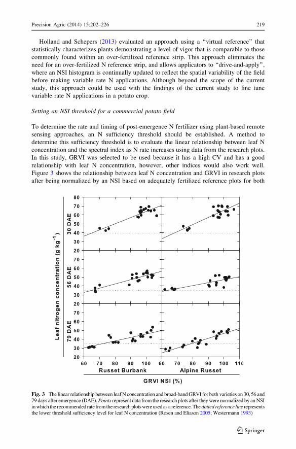
Figure 3 shows the relationship between leaf N concentration and GRVI in research plots

after being normalized by an NSI based on adequately fertilized reference plots for both

Fig. 3 The linear relationship between leaf N concentration and broad-band GRVI for both varieties on 30, 56 and79 days after emergence (DAE). Points represent data from the research plots after they were normalized by an NSIin which the recommended rate from the research plots were used as a reference. The dotted reference line representsthe lower threshold sufficiency level for leaf N concentration (Rosen and Eliason 2005; Westermann 1993)

Precision Agric (2014) 15:202–226 219

123

varieties and all three image dates. The lower threshold sufficiency level for leaf N con-

centration is 40 g kg-1 at 30 DAE and 35 g kg-1 at 56 and 79 DAE (Rosen and Eliason

2005; Westermann 1993). These threshold levels are represented in Fig. 3 by the hori-

zontal dotted lines in each plot. The lower threshold sufficiency level for GRVI NSI is

assumed to be the point in which the linear model crosses below the leaf N concentration

threshold. The GRVI NSI level at the point in which this occurred was between *66 %

(on 30 DAE for RB) and *80 % (on 79 DAE for AR), depending on growth stage and

variety (Fig. 3). In order to be confident that yields will not suffer because of underesti-

mation of actual N stress, the less conservative 80 % GRVI NSI value could be chosen as

the lower threshold sufficiency level. Therefore, a plant with a GRVI NSI value below

80 % should receive supplemental post-emergence N fertilizer in order to optimize yields.

The commercial field was over-fertilized throughout the season, and there was very

little N stress throughout the field. Using the recommended rate from the research plots as

an NSI reference, GRVI resulted in mean NSI values well above 100 % on most mea-

surement dates; there were very few pixels below 100 % (Tables 7, 8; Fig. 2). However,

these data can be used to show which areas in the commercial field are most unsuitable for

supplemental N fertilizer applications by using an over-sufficiency threshold.

Because it was determined that GRVI has a lower threshold sufficiency level of 80 %, a

symmetrical difference above the 100 % reference level (i.e. 120 %) was determined to be

the threshold at which crop N was over-sufficient (for comparison purposes, a vertical

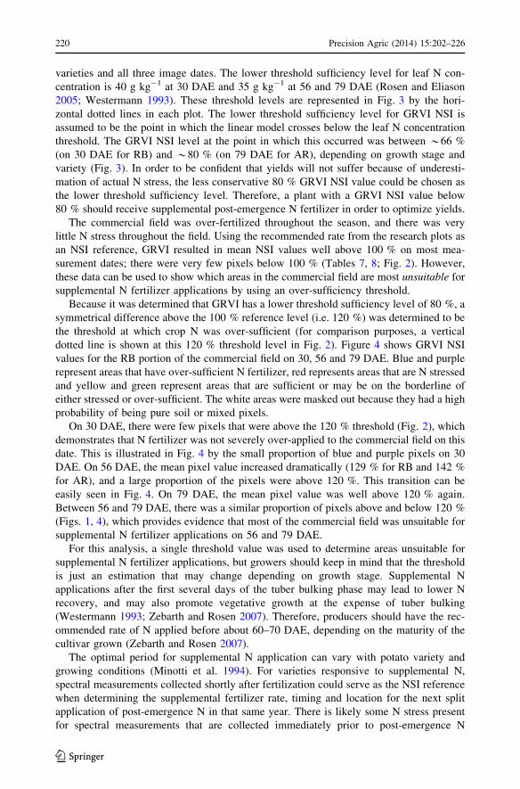
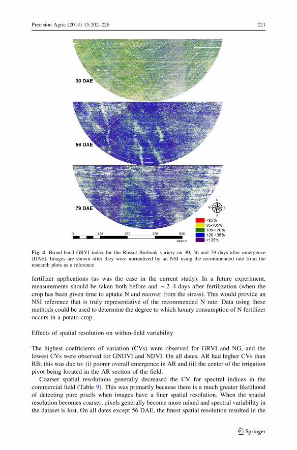
dotted line is shown at this 120 % threshold level in Fig. 2). Figure 4 shows GRVI NSI

values for the RB portion of the commercial field on 30, 56 and 79 DAE. Blue and purple

represent areas that have over-sufficient N fertilizer, red represents areas that are N stressed

and yellow and green represent areas that are sufficient or may be on the borderline of

either stressed or over-sufficient. The white areas were masked out because they had a high

probability of being pure soil or mixed pixels.

On 30 DAE, there were few pixels that were above the 120 % threshold (Fig. 2), which

demonstrates that N fertilizer was not severely over-applied to the commercial field on this

date. This is illustrated in Fig. 4 by the small proportion of blue and purple pixels on 30

DAE. On 56 DAE, the mean pixel value increased dramatically (129 % for RB and 142 %

for AR), and a large proportion of the pixels were above 120 %. This transition can be

easily seen in Fig. 4. On 79 DAE, the mean pixel value was well above 120 % again.

Between 56 and 79 DAE, there was a similar proportion of pixels above and below 120 %

(Figs. 1, 4), which provides evidence that most of the commercial field was unsuitable for

supplemental N fertilizer applications on 56 and 79 DAE.

For this analysis, a single threshold value was used to determine areas unsuitable for

supplemental N fertilizer applications, but growers should keep in mind that the threshold

is just an estimation that may change depending on growth stage. Supplemental N

applications after the first several days of the tuber bulking phase may lead to lower N

recovery, and may also promote vegetative growth at the expense of tuber bulking

(Westermann 1993; Zebarth and Rosen 2007). Therefore, producers should have the rec-

ommended rate of N applied before about 60–70 DAE, depending on the maturity of the

cultivar grown (Zebarth and Rosen 2007).

The optimal period for supplemental N application can vary with potato variety and

growing conditions (Minotti et al. 1994). For varieties responsive to supplemental N,

spectral measurements collected shortly after fertilization could serve as the NSI reference

when determining the supplemental fertilizer rate, timing and location for the next split

application of post-emergence N in that same year. There is likely some N stress present

for spectral measurements that are collected immediately prior to post-emergence N

220 Precision Agric (2014) 15:202–226

123

fertilizer applications (as was the case in the current study). In a future experiment,

measurements should be taken both before and *2–4 days after fertilization (when the

crop has been given time to uptake N and recover from the stress). This would provide an

NSI reference that is truly representative of the recommended N rate. Data using these

methods could be used to determine the degree to which luxury consumption of N fertilizer

occurs in a potato crop.

Effects of spatial resolution on within-field variability

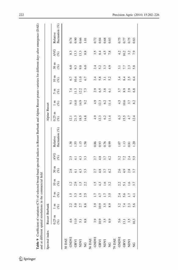
The highest coefficients of variation (CVs) were observed for GRVI and NG, and the

lowest CVs were observed for GNDVI and NDVI. On all dates, AR had higher CVs than

RB; this was due to: (i) poorer overall emergence in AR and (ii) the center of the irrigation

pivot being located in the AR section of the field.

Coarser spatial resolutions generally decreased the CV for spectral indices in the

commercial field (Table 9). This was primarily because there is a much greater likelihood

of detecting pure pixels when images have a finer spatial resolution. When the spatial

resolution becomes coarser, pixels generally become more mixed and spectral variability in

the dataset is lost. On all dates except 56 DAE, the finest spatial resolution resulted in the

Fig. 4 Broad-band GRVI index for the Russet Burbank variety on 30, 56 and 79 days after emergence(DAE). Images are shown after they were normalized by an NSI using the recommended rate from theresearch plots as a reference

Precision Agric (2014) 15:202–226 221

123

Ta

ble

9C

oef

fici

ent

of

var

iati

on

(CV

)o

fse

lect

edb

road

-ban

dsp

ectr

alin

dic

esin

Ru

sset

Burb

ank

and

Alp

ine

Russ

etp

ota

tov

arie

ties

for

dif

fere

nt

day

saf

ter

emer

gen

ce(D

AE

)an

dat

dif

fere

nt

spat

ial

reso

luti

on

sin

the

com

mer

cial

fiel

d

Sp

ectr

alin

dex

Ru

sset

Bu

rban

kA

lpin

eR

uss

et

0.2

5m

(%)

1m

(%)

5m

(%)

10

m(%

)3

0m

(%)

AV

G(%

)R

elat

ive

flu

ctu

atio

n(%

)0

.25

m(%

)1

m(%

)5

m(%

)1

0m

(%)

30

m(%

)A

VG

(%)

Rel

ativ

efl

uct

uat

ion

(%)

30

DA

E

GN

DV

I4

.62

.21

.51

.22

.82

.51

.38

12

.19

.17

.46

.76

.08

.30

.74

GR

VI

11

.05

.03

.32

.94

.14

.11

.55

21

.31

4.0

11

.31

0.4

9.3

13

.30

.90

ND

VI

5.1

2.7

1.9

1.5

4.3

4.3

1.1

51

8.5

14

.91

2.2

11

.09

.81

3.3

0.6

6

NG

8.8

8.8

2.5

2.2

3.3

3.3

1.5

81

4.8

9.2

7.3

6.7

6.0

8.8

1.0

1

56

DA

E

GN

DV

I3

.93

.91

.71

.52

.72

.70

.86

4.9

4.9

2.9

2.4

2.4

3.5

0.7

2

GR

VI

10

.91

0.9

4.7

4.3

4.8

4.8

0.9

31

2.3

12

.36

.55

.85

.28

.40

.84

ND

VI

3.5

3.5

1.7

1.6

3.7

3.7

0.7

66

.26

.23

.83

.13

.34

.50

.68

NG

8.9

8.9

3.5

3.2

4.2

4.2

0.9

91

1.4

11

.46

.15

.24

.97

.80

.83

79

DA

E

GN

DV

I5

.63

.22

.42

.22

.63

.21

.07

6.3

4.5

3.7

3.4

3.1

4.2

0.7

5

GR

VI

13

.17

.45

.65

.14

.97

.21

.13

15

.51

0.6

8.9

8.4

7.7

10

.20

.77

ND

VI

3.5

2.3

1.7

1.6

2.8

2.4

0.8

14

.73

.72

.92

.52

.33

.20

.75

NG

10

.35

.64

.13

.73

.75

.51

.20

12

.48

.26

.86

.45

.87

.90

.83

222 Precision Agric (2014) 15:202–226

123

highest CV (Table 9). On 56 DAE, the CVs between the images with 0.25 m and 1-m

spatial resolutions were the same after rounding. There was *1.0 m between rows of the

planted potato crop, so for the images with a 0.25-m spatial resolution, four pixels covered

the width of an entire crop row (including the inter-row). Because mixed pixels were not

masked before this analysis, pixels could be a representation of the crop rows, inter-rows or

both. Therefore, it is reasonable to suggest that the variability on the dates before and after

56 DAE is due to bare soil showing through the crop canopy. The images with the 0.25-m

spatial resolution could detect this variability, and the images with the 1-m spatial reso-

lution could not.

On 56 DAE, however, the imagery with the 0.25-m spatial resolution was not able to

detect any more variability than was detected by the imagery with the 1-m spatial reso-

lution. This suggests that vegetative growth likely peaked on *56 DAE and canopy cover

was at or near 100 %, which resulted in not being able to detect any additional spectral

information with sub-meter spatial resolution imagery. Before this date, vegetative growth

was still progressing, and after this date, the plant canopy began to fall over and, by 79

DAE, senesce. Figure 1 illustrates how additional information was detected by the 0.25-m

spatial resolution images on 30 and 79 DAE, but not on 56 DAE (the crop rows were

planted West-East). Because there was only *1 m between crop rows, factors detectable

at a spatial scale greater than or equal to 1 m were the cause of the lost information for the

images that had spatial resolutions greater than 1 m. It is reasonable to assume that an

image that has a lower CV has a greater proportion of mixed pixels. On dates before and

after peak vegetative growth (which was estimated to be *56 DAE in the current study),

images with finer spatial resolutions have a higher CV, and therefore, also have a greater

proportion of pure pixels. Thus, there is value in obtaining imagery at sub-meter spatial

resolutions in order to determine supplemental N fertilizer applications, especially at

growth stages before and after *56 DAE in the current study (Fig. 1).

The RF of the CVs over spatial resolutions was lowest for GNDVI and NDVI (Table 9).

Low RF values are most desirable since they indicate consistent values over spatial res-

olutions. Low variability over spatial resolutions is important for a spectral index because

it demonstrates its robustness over a variety of circumstances. Spectral indices with higher

RFs are more likely to have NSI thresholds (e.g. 80 % for GRVI) change as the spatial

resolution changes. If a grower uses imagery with a coarser spatial resolution than 0.25 m,

less information about the crop canopy will be sacrificed if indices with low RF values are

used; however, the ability of the indices used to predict crop N stress should also be a

strong consideration when selecting a spectral index to be used to determine the rate and

timings of split-applications of N fertilizer. Because GRVI had high CV and moderate RF

values, it was determined to be a good spectral index to use for N stress determination

using imagery with different spatial resolutions.

Conclusions

This study showed that high resolution (0.25 m) broad-band imagery can be a useful tool

for detecting N stress in a potato crop while accounting for within-field spatial variability.

Broad-band spectral data shows promise for helping to improve N fertilizer management

while reducing groundwater nitrate contamination due to over-application. Of the broad-

band spectral indices tested within measurement dates from the research plots, GRVI

predicted leaf N concentration with the most certainty over all image dates, and actually

performed better than the chlorophyll meter in some circumstances; GRVI also had the

Precision Agric (2014) 15:202–226 223

123

highest coefficient of variation from the commercial field. Because N was applied at a rate

greater than that of regionally recommended guidelines, a GRVI NSI threshold of 120 %

was able to determine the areas of the commercial field that were most unsuitable for

supplemental N fertilizer applications when the recommended rate and timing from the

research plot was used as a reference. In situations where N is applied more sparingly, a

GRVI NSI threshold of 80 % should be used to identify areas that are most suitable for

supplemental N fertilizer. Because of differences in potato variety, growth stage or other

local conditions, spectral data should be normalized so supplemental N rates and timings

can be determined at an accurate level. Different NSI threshold levels should be estab-

lished depending on: (1) the inherent variability/CV of the spectral index, (2) the NSI

reference used and (3) the growth stage.

Acknowledgments Financial support for this project was provided by the Binational AgriculturalResearch and Development Fund (through Research Grant Award No. IS-4255-09), the Hueg-HarrisonFellowship and the Minnesota Area II Potato Growers. The Upper Midwest Aerospace Consortium (UMAC)at the University of North Dakota is acknowledged for acquiring the imagery for this study; also, K & OFarms is acknowledged for allowing us to work with them on this study.

References

Bailey, R. J. (2000). Practical use of soil water measurement in potato production. In A. J. Haverkort & D.K. L. MacKerron (Eds.), Management of nitrogen and water in potato production (pp. 206–218).Wageningen: Wageningen Academic Publishers.

Barnes, E. M., Clarke, T. R., Richards, S. E., Colaizzi, P. D., Haberland, J., Kostrzewski, M., et al. (2000).Coincident detection of crop water stress, nitrogen status and canopy density using ground basedmultispectral data. Paper presented at the Proceedings of the 5th International Conference on PrecisionAgriculture, Bloomington, MN. 16–19 July 2000. ASA, CSSA, and SSSA, Madison, WI.

Blackmer, T. M., & Schepers, J. S. (1995). Use of chlorophyll meter to monitor nitrogen status and schedulefertigation for corn. Journal of Production Agriculture, 8, 56–60.

Canter, L. W. (1997). Nitrates in groundwater. Boca Raton, FL: CRC Press Inc.Carlson, R. M. (1986). Continuous flow reduction of nitrate to ammonia with granular zinc. Analytical

Chemistry, 58, 1590–1591.Carlson, R. M., Cabrera, R. I., Paul, J. L., Quick, J., & Evans, R. Y. (1990). Rapid direct determination of

ammonium and nitrate in soil and plant tissue extracts. Communications in Soil Science and PlantAnalysis, 21, 1519–1529.

Dean, B. B. (1994). Managing the potato production system. New York: Food Products Press.Denuit, J. P., Olivier, M., Goffaux, M. J., Herman, J. L., Goffart, J. P., Destain, J. P., et al. (2002).

Management of nitrogen fertilization of winter wheat and potato crops using the chlorophyll meter forcrop nitrogen status assessment. Agronomie, 22, 847–854.

Engel, D., Foster, R., Maynard, E., Weinzierl, R., Babadoost, M., O’Malley, P., et al. (2012). Midwestvegetable production guide for commercial growers. Publ. BU-07094-S. Saint Paul, MN: Univ. ofMinnesota Extension Service.

EPA. (2009). National primary drinking water regulations. (Publ. 816-F-09-004).Errebhi, M., Rosen, C. J., Gupta, S. C., & Birong, D. E. (1998). Potato yield response and nitrate leaching as

influenced by nitrogen management. Agronomy Journal, 90, 10–15.Gitelson, A. A., Kaufman, Y. J., & Merzlyak, M. N. (1996). Use of a green channel in remote sensing of

global vegetation from EOS-MODIS. Remote Sensing of Environment, 58, 289–298.Hansen, P. M., & Schjoerring, J. K. (2003). Reflectance measurement of canopy biomass and nitrogen status

in wheat crops using normalized difference vegetation indices and partial least squares regression.Remote Sensing of Environment, 86, 542–553.

Holland, K. H., & Schepers, J. S. (2013). Use of a virtual-reference concept to interpret active crop canopysensor data. Precision Agriculture, 14, 71–85.

Horneck, D. A., & Miller, R. O. (1997). Determination of total nitrogen in plant tissue. In Y. P. Kalra (Ed.),Handbook of reference methods for plant analysis (pp. 75–84). Boston, FL: CRC Press.

Huete, A. (1988). A soil adjusted vegetation index (SAVI). Remote Sensing of Environment, 25, 295–309.

224 Precision Agric (2014) 15:202–226

123

Jain, N., Ray, S. S., Singh, J. P., & Panigrahy, S. (2007). Use of hyperspectral data to assess the effects ofdifferent nitrogen applications on a potato crop. Precision Agriculture, 8, 225–239.

Lesczynski, D. B., & Tanner, C. B. (1976). Seasonal variation of root distribution of irrigated, field-grownRusset Burbank potato. American Journal of Potato Research, 53, 69–78.

Lynch, J., Marschner, P., & Rengel, Z. (2012). Effect of internal and external factors on root growth anddevelopment. In P. Marschner (Ed.), Marschner’s mineral nutrition of higher plants (3rd ed.,pp. 331–346). San Diego, CA: Academic Press.

Meisinger, J. J., Schepers, J. S., & Raun, W. R. (2008). Crop nitrogen requirement and fertilization. In J.S. Schepers & W. Raun (Eds.), Nitrogen in agricultural systems (pp. 563–612). Madison, WI: ASA-CSSA-SSSA.

Mendez Mediavilla, F. A., Landram, F., & Shah, V. (2008). A comparison of the coefficient of predictivepower, the coefficient of determination and AIC for linear regression. Paper presented at the Pro-ceedings of the 39th Annual Meeting of the Decision Sciences Institute, Atlanta, 1261–1266.

Miao, Y., Mulla, D. J., Randall, G. W., Vetsch, J. A., & Vintila, R. (2009). Combining chlorophyll meterreadings and high spatial resolution remote sensing images for in-season site-specific nitrogen man-agement of corn. Precision Agriculture, 10, 45–62.

Midwest Regional Climate Center. Climate of the Midwest. Retrieved August 11 2012, from http://mcc.sws.uiuc.edu/climate_midwest.

Minotti, P. L., Halseth, D. E., & Sieczka, J. B. (1994). Field chlorophyll measurements to assess the nitrogenstatus of potato varieties. HortScience, 29, 1497–1500.

Nigon, T. J. (2012a). Hyperspectral imagery for detecting nitrogen stress in two potato varieties. In Aerialimagery and other non-invasive approaches to detect nitrogen and water stress in a potato crop.Masters thesis. (pp.111–159). University of Minnesota Digital Conservancy, http://purl.umn.edu/143695.

Nigon, T. J. (2012b). Irrigation and nitrogen management effects on potato nitrogen use indices and tuberyield and quality. In Aerial imagery and other non-invasive approaches to detect nitrogen and waterstress in a potato crop. Masters thesis. (pp. 41-77). University of Minnesota Digital Conservancy,http://purl.umn.edu/143695.

Olivier, M., Goffart, J. P., & Ledent, J. F. (2006). Threshold value for chlorophyll meter as decision tool fornitrogen management of potato. Agronomy Journal, 98, 496–506.

Peterson, T. A., Blackmer, T. M., Francis, D. D., & Schepers, J. S. (1993). Using a chlorophyll meter toimprove N management. Publ. G93-1171A. Lincoln, NE: University of Nebraska CooperativeExtension Service.

Qi, J., Chehbouni, A., Huete, A. R., Kerr, Y. H., & Sorooshian, S. (1994). A modified soil adjustedvegetation index. Remote Sensing of Environment, 48, 119–126.

Rondeaux, G., Steven, M., & Baret, F. (1996). Optimization of soil-adjusted vegetation indices. RemoteSensing of Environment, 55, 95–107.

Rosen, C. J., & Bierman, P. M. (2008). Best management practices for nitrogen use: Irrigated potatoes.Publ. 08559. Saint Paul, MN: University of Minnesota Extension Service.

Rosen, C. J., & Eliason, R. (2005). Nutrient management for commercial fruit & vegetable crops inMinnesota. Publ. BU-05886. Saint Paul, MN: University of Minnesota Extension Service.

Rouse, J. W., Haas, R. H., Schell, J. A., Deering, D. W., & Harlan, J. C. (1974). Monitoring the vernaladvancement of retrogradation (green wave effect) of natural vegetation. In: NASA/GSFC FinalReport, Greenbelt, MD, USA, 1-137.

SAS Institute. 2008. Release 9.2 ed. SAS Inst., Cary, NC.Saxton, A. M. (1998). A macro for converting mean separation output to letter groupings in proc mixed.

Proc. 23rd SAS Users Group International Conference (pp. 1243–1246). SAS Institute: Cary, NC.Shapiro, C. A., Schepers, J. S., Francis, D. D., & Shanahan, J. F. (2006). Using a chlorophyll meter to

improve N management. Publ. G1632. Lincoln, NE: Univ. of Nebraska Coop. Ext. Service.Sripada, R. P., Heiniger, R. W., White, J. G., & Meijer, A. D. (2006). Aerial color infrared photography for

determining early in-season nitrogen requirements in corn. Agronomy Journal, 98, 968–977.Sripada, R. P., Schmidt, J. P., Dellinger, A. E., & Beegle, D. B. (2008). Evaluating multiple indices from a

canopy reflectance sensor to estimate corn N requirements. Agronomy Journal, 100, 1553–1561.Stroppiana, D., Fava, F., Boschetti, M., & Brivio, P. A. (2012). Estimation of nitrogen content in crops and

pastures. In P. S. Thenkabail, J. G. Lyon, & A. Huete (Eds.), Hyperspectral remote sensing of vege-tation (pp. 245–262). Boca Raton, FL: CRC Press.

Tremblay, N., Fallon, E., & Ziadi, N. (2011). Sensing of crop nitrogen status: Opportunities, tools, limi-tations, and supporting information requirements. HortTechnology, 21, 274–281.

Varvel, G. E., Schepers, J. S., & Francis, D. D. (1997). Ability for in-season correction of nitrogen defi-ciency in corn using chlorophyll meters. Soil Science Society of America Journal, 61, 1233–1239.

Precision Agric (2014) 15:202–226 225

123

Waddell, J. T., Gupta, S. C., Moncrief, J. F., Rosen, C. J., & Steele, D. D. (2000). Irrigation- and nitrogen-management impacts on nitrate leaching under potato. Journal of Environmental Quality, 29, 251–261.

Westermann, D. T. (1993). Fertility management. In R. C. Rowe (Ed.), Potato health management (pp.77–86). St. Paul, MN: The American Phytopathological Society.

Westermann, D. T., Kleinkopf, G. E., & Porter, L. K. (1988). Nitrogen fertilizer efficiencies on potatoes.American Journal of Potato Research, 65, 377–386.

Whitworth, J. L., Novy, R. G., Stark, J. C., Pavek, J. J., Corsini, D. L., Love, S. L., et al. (2011). AlpineRusset: A potato cultivar having long tuber dormancy making it suitable for processing from long-termstorage. American Journal of Potato Research, 88, 256–268.

Woodcock, C. E., & Strahler, A. H. (1987). The factor of scale in remote sensing. Remote Sensing ofEnvironment, 21, 311–332.

Wright, J. (2002). Irrigation scheduling checkbook method. Publ. FO-01322. Saint Paul, MN: University ofMinnesota Extension Service.

Zebarth, B. J., & Rosen, C. J. (2007). Research perspective on nitrogen BMP development for potato.American Journal of Potato Research, 84, 283–294.

Zebarth, B. J., Younie, M., Paul, J. W., & Bittman, S. (2002). Evaluation of leaf chlorophyll index formaking fertilizer nitrogen recommendations for silage corn in a high fertility environment. Commu-nications in Soil Science and Plant Analysis, 33, 665–684.

Zhang, X., Streeter, C., Kim, H., & Olsen, D. (2011). Near real-time meter-resolution airborne imagery forprecision agriculture: AEROCam. GeoCarto International, 26, 537–551.

Zvomuya, F., Rosen, C. J., Russelle, M. P., & Gupta, S. C. (2003). Nitrate leaching and nitrogen recoveryfollowing application of polyolefin-coated urea to potato. Journal of Environmental Quality, 32,480–489.

226 Precision Agric (2014) 15:202–226

123