Embed Size (px)
Citation preview

Faculty of Science and Technology
MASTER’S THESIS
Study program/ Specialization:
Petroleum Engineering
Reservoir technology
Spring semester, 2012
Open
Writer: Ole Andreas Knappskog
………………………………………… (Writer’s signature)
Faculty supervisor: Hans Kleppe (University of Stavanger)
External supervisor: Robert W. Moe (ConocoPhillips)
Title of thesis: Evaluation of WAG injection at Ekofisk
Credits (ECTS): 30
Key words:
-HC WAG
-SORM
-Trapped gas
-Hysteresis effect
-Minimum miscibility pressure
-Minimum miscibility enrichment
Pages: …………………
+ enclosure: …………
Stavanger, ………………..
Date/year

2
Master’s Thesis
Evaluation of WAG injection at
Ekofisk
by
Ole Andreas Knappskog
June 15th, 2012
University of Stavanger
Faculty of Science and Technology
Petroleum Engineering, Reservoir Technology
3
Abstract
In the North Sea many fields are water flooded. Subsequent to water flooding large amounts
of water flood residual oil will be left in reservoirs. The challenge is how to improve the oil
recovery. On the Ekofisk field such a challenge is to be addressed. The entire reservoir on
the Ekofisk field is currently water flooded. The current plan is to continue water injection
until the end of license in 2028. To improve oil recovery, EOR mechanisms have been
proposed. The EOR mechanism hydrocarbon water-alternating gas has shown good
potential and will be studied in this thesis.
The main purpose of this thesis is to evaluate WAG injection at Ekofisk. A number of
factors may affect WAG performance, in this study the importance of some of these will be
evaluated through simulation work. Miscibility evaluation is performed using a slim-tube
simulation model. Mechanistic models are further used to evaluate other key parameters
such as trapped gas saturation, hysteresis effect, fracture-matrix system and SORM. Finally
a sector model is used to optimize WAG ratios and WAG slug sizes, and to make a
comparison of WAG scenarios to a water flood case.
The slim-tube simulation work resulted in the conclusion to use immiscible WAG injection
by dry hydrocarbon gas, because of high minimum miscibility pressure and minimum
miscibility enrichment.
Mechanistic simulations indicated that trapped gas and SORM should be included in WAG-
modeling to avoid over prediction of recoveries for a WAG applications.
Sector simulations showed incremental oil potential to the water flood case for all WAG
scenarios. WAG ratio of 1 to 2 gave the largest increase with 8.4 million BOE. Increasing
WAG ratio showed decreasing potential. Similar, the WAG slug size of 0.4 pore volumes
was best with 4.4 million BOE incremental to the base case. WAG slug sizes showed
decreasing potential with decreasing slug sizes.
The results from the sector model indicated the need of optimization of the total volume of
gas injected for the WAG application, which is recommended for further studies, together
with introducing local grid refinement to avoid numerical dispersion and instability
problems.

4
Table of contents
i. Abstract 3
ii. Table of contents 4
iii. Acknowledgements 7
iv. List of figures 8
v. List of tables 10
1 Introduction ................................................................................................................... 11
2 Ekofisk field history and background............................................................................ 13
3 Literature review ........................................................................................................... 25
4 Theory............................................................................................................................ 32
4.1 Rock properties ....................................................................................................... 32
4.1.1 Porosity ............................................................................................................ 32
4.1.2 Absolute permeability ..................................................................................... 32
4.1.3 Effective permeability ..................................................................................... 33
4.2 Relative permeability .............................................................................................. 33
4.2.1 Two-phase relative permeability ..................................................................... 34
4.2.2 Three-phase relative permeability ................................................................... 36
4.2.2.1 Stone’s models ............................................................................................. 37
4.3 Surface and interfacial tension ................................................................................ 38
4.4 Rock wettability ...................................................................................................... 38
4.5 Capillary pressure ................................................................................................... 41
4.6 Trapped gas saturation and hysteresis effect .......................................................... 44
4.6.1 Introduction to trapped gas saturation and hysteresis...................................... 44
4.6.2 Trapped gas saturation correlations and hysteresis models in PSim ............... 45
4.6.2.1 Land’s correlation ........................................................................................ 45
4.6.2.2 Coats correlation .......................................................................................... 47
4.6.3 Other relative permeability hysteresis models ................................................ 47
4.6.3.1 Carlson hysteresis model ............................................................................. 48
4.6.3.2 Killough hysteresis model ........................................................................... 49

5
4.6.3.3 Skauge and Larsen three-phase hysteresis model ........................................ 49
4.7 Miscible flood residual oil saturation (SORM) ...................................................... 51
4.8 Matrix-fracture mechanisms ................................................................................... 52
4.9 Recovery mechanisms relevant to WAG ................................................................ 54
4.9.1 Oil recovery mechanisms for water injection .................................................. 54
4.9.1.1 Gravitational displacement .......................................................................... 54
4.9.1.2 Capillary displacement - spontaneous imbibition ........................................ 55
4.9.1.3 Viscous displacement .................................................................................. 56
4.9.2 Oil recovery mechanisms for gas injection ..................................................... 56
4.9.2.1 Vaporizing gas drive / oil stripping ............................................................. 57
4.9.2.2 Condensation gas-drive / oil swelling .......................................................... 57
4.9.2.3 Gravity drainage .......................................................................................... 58
4.9.2.4 Molecular diffusion...................................................................................... 58
4.9.2.5 Combination of vaporizing and condensing mechanisms ........................... 59
4.9.3 Capillary continuity ......................................................................................... 59
4.10 Miscible and immiscible WAG ........................................................................... 60
4.10.1 Miscible displacement ..................................................................................... 60
4.10.1.1 First contact miscibility ............................................................................... 60
4.10.1.2 Multi-contact miscibility.............................................................................. 61
4.10.2 Immiscible displacement ................................................................................. 61
4.10.3 Evaluation of miscibility ................................................................................. 62
4.10.3.1 Minimum miscibility pressure (MMP) ........................................................ 62
4.10.3.2 Minimum miscibility enrichment (MME) ................................................... 63
4.10.3.3 Evaluation of MMP and MME .................................................................... 63
4.10.3.4 Slim-tube tests.............................................................................................. 64
4.11 Introduction to the numerical reservoir simulation tool (PSim) ......................... 65
5 Slim-tube modeling ....................................................................................................... 67
5.1 Description of the slim tube model ......................................................................... 67
5.2 Methodology for slim tube model .......................................................................... 69
5.2.1 Methodology minimum miscibility pressure .................................................. 69
5.2.2 Methodology minimum miscibility enrichment .............................................. 70

6
5.3 Results and discussion of slim-tube simulations .................................................... 72
5.3.1 Minimum miscibility pressure ......................................................................... 72
5.3.2 Minimum miscibility enrichment .................................................................... 76
6 Mechanistic modeling ................................................................................................... 79
6.1 Description of mechanistic models ......................................................................... 79
6.2 Methodology for mechanistic modeling ................................................................. 85
6.2.1 Trapped gas saturation and relative permeability hysteresis effect ................. 85
6.2.2 Matrix-fracture systems ................................................................................... 86
6.2.3 Miscible flood residual oil saturation .............................................................. 90
6.3 Results and discussion of mechanistic simulations ................................................ 91
6.3.1 Trapped gas saturation and relative permeability hysteresis effect ................. 91
6.3.2 Matrix-fracture systems ................................................................................... 96
6.3.3 Miscible flood residual oil saturation ............................................................ 101
7 Sector modeling ........................................................................................................... 107
7.1 Description and methodology for sector model .................................................... 108
7.2 Results and discussion of sector simulations ........................................................ 113
7.2.1 WAG-ratio ..................................................................................................... 113
7.2.2 WAG slug sizes ............................................................................................. 115
8 Conclusion ................................................................................................................... 117
9 Abbreviations and symbols ......................................................................................... 119
10 References ................................................................................................................... 122
11 Appendices .................................................................................................................. 128

7
Acknowledgements
First of all I would like to thank ConocoPhillips for providing me with an interesting and
challenging master thesis and for giving me access to all their information and studies. I
genuinely appreciate the opportunity to work at ConocoPhillips with some of the best
people in this field.
I would especially like to extend my sincere and gratitude to my external supervisor at
ConocoPhillips, Robert W. Moe, who has provided me with great guidance and support
throughout the process of writing this thesis. He has patiently answered all questions and
given me theoretical insight in the difficult parts of my study. I am also grateful for the
valuable assistance from the Field Management group, from WAG specialist Arvid Østhus,
and from Murali Muralidharan and Russ Bone in ConocoPhillips USA.
Further I would like to give thanks to my internal supervisor at the University of Stavanger,
Professor Hans Kleppe for his guidance.
During my time at ConocoPhillips I have enjoyed meeting the other graduates for lunch and
coffee breaks. The socialization with you guys has lighted up my workday.
Finally, I thank my family, especially Marija, whose daily support and encouragement I
could not do without.
Regards,
Ole Andreas Knappskog,
Stavanger, 15.juni 2012

8
List of figures
Chapter 2 Figure 2.1: Location of the Greater Ekofisk Area, where the Ekofisk field is one of four producing fields .... 13
Figure 2.2: Geological time scale of important geological events for the Ekofisk field ................................. 17
Figure 2.3: Formations of the Ekofisk field (Sulak, 1990) .............................................................................. 19
Figure 2.4: Ekofisk field-wide GOR history .................................................................................................... 20
Figure 2.5: Subsidence of Ekofisk seafloor .................................................................................................... 21
Figure 2.6: Subsidence rate history at Ekofisk ............................................................................................... 22
Figure 2.7: Tectonic and stylolite associated fractures ................................................................................. 23
Chapter 3 Figure 3.1: Cumulative number of worldwide WAG applications from the first project in 1957 to 1996
(Christensen, et al., 2001) .................................................................................................................... 25
Figure 3.2: Full field WAG-simulation versus long term water flood production forecast (Østhus, 1998 ) ... 30
Chapter 4 Figure 4.1: Example of hysteresis affected gas relative permeability imbibition curve ................................ 34
Figure 4.2: Illustration of the shape of (a) water-oil relative permeability curves, and corresponding end-
point saturations (b) gas-oil relative permeability curves, and corresponding end-point saturations 35
Figure 4.3: Three-phase flow in a WAG-system (Skauge, et al., 2007) .......................................................... 36
Figure 4.4: Interfacial forces when water and oil are in contact with a solid rock in a water-wet-system ... 39
Figure 4.5: Rocks wetting preferences based on contact angle (Ursin, et al., 1997) ..................................... 39
Figure 4.6 Fluid distributions within water-wet and oil-wet systems (Green, et al., 1998)........................... 40
Figure 4.7: Wettability effect on relative permeability curves for (a) water-wet systems and (b) oil-wet
systems ................................................................................................................................................ 40
Figure 4.8: Radius of curvature on a curved surface (Ursin, et al., 1997) ...................................................... 41
Figure 4.9: Two immiscible fluids forming an idealized spherical curvature (Ursin, et al., 1997) .................. 42
Figure 4.10: Illustration of water-oil capillary pressure curves ..................................................................... 43
Figure 4.11: Carlson hysteresis affected non-wetting phase relative permeability curves (Kossack, 2000) .. 48
Figure 4.12: Killough hysteresis affected non-wetting phase relative permeability curves (Killough, 1976) 49
Figure 4.13: Skauge and Larsen hysteresis affected gas relative permeability curves, changing between a
high and a low mobility envelope. (Larsen, et al., 1995) ..................................................................... 50
Figure 4.14: Skauge and Larsen water relative permeability curves, changing between a high mobility curve
and a low mobility curve in correspondence with the gas-phase envelops in figure 4.13. (Larsen, et
al., 1995) .............................................................................................................................................. 51
Figure 4.15: Capillary imbibition as a function of wettability ....................................................................... 56
Chapter 5 Figure 5.1: Illustration of slim-tube model after some time of gas injection ................................................ 67
F ............................................................................................................ 73
F, zoomed to the break-over pressure region ...................................... 73
Figure 5.4: MMP evaluation at different temperatures ................................................................................ 74
Figure 5.5: The pressure range which MMP was determined, for different temperatures ........................... 75
F
F ................................................................................................................................................... 76
F and constant operating pressure of 6000
psia. ..................................................................................................................................................... 77

9
Chapter 6 Figure 6.1: Input matrix (a) gas-oil and (b) water-oil relative permeability curves for the mechanistic
models ................................................................................................................................................. 80
Figure 6.2: Matrix water-oil capillary pressure curves for the mechanistic models ...................................... 81
Figure 6.3: Fracture (a) water-oil and (b) gas-oil relative permeability curves for matrix-fracture models .. 82
Figure 6.4: Oil recovery and reservoir pressure for the homogeneous matrix model ................................... 84
Figure 6.5: 3-layer fracture model in the xz-plane ........................................................................................ 87
Figure 6.6: Six-layer fracture model shown in the zx-plane .......................................................................... 88
Figure 6.7: Discontinuous fracture model in the xz-plane ............................................................................. 89
Figure 6.8: 9-block fracture model in the xz-plane ........................................................................................ 90
Figure 6.9: Land and Coats trapped gas saturation as function of maximum historical gas saturation for
reference grid block (18,1,18) .............................................................................................................. 92
Figure 6.10: Gas relative permeability curves for Coats and Lands correlations with input maximum trapped
gas saturation of 0.2 based on data from the reference grid block (18,1,18) ...................................... 93
Figure 6.11: Trapped gas correlations and different Sgr-input values compared to reported and laboratory
data on trapped gas ............................................................................................................................. 94
Figure 6.12: Impact of trapped gas on oil recovery for WAG-displacement .................................................. 95
Figure 6.13: Oil recovery for the matrix-fracture models perforated in matrix only .................................... 97
Figure 6.14: Gas saturation in the 3-layer fracture model ............................................................................ 98
Figure 6.15: Gas saturation in the 6-layer fracture model ............................................................................ 98
Figure 6.16: Gas saturation in the 9-block fracture model ............................................................................ 99
Figure 6.17: Oil recovery for the matrix-fracture models perforated in matrix and fracture grid blocks .... 100
Figure 6.18: Oil recovery for the different SORM options in PSim, and a run without SORM ..................... 103
Figure 6.19: Oil saturation as a function of time in the reference grid block (18,1,18) for the two available
SORM options in PSim, and the run without SORM .......................................................................... 103
Figure 6.20: Effect of different input SORM values to oil recovery for SORM Sotrig option ....................... 104
Figure 6.21: Oil saturation as a function of time for different SORM input values for the reference grid
block .................................................................................................................................................. 105
Chapter 7 Figure 7.1: Ekofisk full field model, illustrating the location of the sector model within the red square .... 107
Figure 7.2: The 22 layers of the sector model ............................................................................................. 109
Figure 7.3: Initial reservoir pressures and distribution of wells and faults in the sector models upper layer 1.
........................................................................................................................................................... 110
Figure 7.4: Oil recovery and average pressure for the base case simulation in the sector model............... 111
Figure 7.5: Cumulative incremental barrels of oil equivalent to water flood base case for different WAG
ratios .................................................................................................................................................. 113
Figure 7.6: Gas saturation and permeability in layer 8 of the sector model during WAG injection ............ 114
Figure 7.7: Cumulative incremental barrels of oil equivalent to water flood base case for different slug sizes
........................................................................................................................................................... 115

10
List of tables
Chapter 3 Table 3.1: Summarize of suggested solutions to prevent hydrate formation problem for WAG injection at
the Ekofisk field (Lekvam, et al., 1997) ................................................................................................ 29
Table 3.2: Composition of injected gas used in previous Ekofisk WAG-simulations (Østhus, 1998 ) ............ 30
Chapter 4 Table 4.1: Wettability preference expressed by contact angle (Ursin, et al., 1997) ...................................... 39
Chapter 5 Table 5.1: The 15 components used in EOS for slim-tube simulations .......................................................... 68
Table 5.2: Composition of Ekofisk dry hydrocarbon gas ............................................................................... 70
Table 5.3: Composition of the NGL added to dry gas in MME evaluations ................................................... 71
Chapter 6 Table 6.1: Matrix properties used in the mechanistic models ...................................................................... 80
Table 6.2: Fracture properties used in the matrix-fracture mechanistic models .......................................... 82
Table 6.3: 7-components EOS ....................................................................................................................... 83
Table 6.4: Oil recoveries for the matrix-fracture models perforated in matrix only ..................................... 97
Table 6.5: Oil recoveries for the matrix-fracture models perforated in both matrix and fractures .............. 99
Table 6.6: Assignment of SORM-values to different grid blocks in sector model based on results from the
matrix-fracture mechanistic models .................................................................................................. 102
Chapter 7 Table 7.1: Barrels of oil equivalent and incremental barrels of oil equivalent to base case for different WAG
ratios for the predictive part from 2011 to 2028 ............................................................................... 114
Table 7.2: Barrels of oil equivalent and incremental barrels of oil equivalent to base case for different slug
sizes with WAG ratio 1:1 for the predictive part from 2011 to 2028 ................................................. 116

11
1 Introduction
Subject and problem statement
In the North Sea many fields are water flooded. Subsequent to water flooding large amounts
of water flood residual oil will be left in reservoirs. The challenge is how to improve the oil
recovery. It has been recognized that there is large potentials for enhanced oil recovery
(EOR). One of the EOR-mechanisms is hydrocarbon water-alternating-gas (HC-WAG)
injection.
On the Ekofisk field such a challenge is to be addressed. The entire reservoir on the Ekofisk
field is currently water flooded, both vertically and laterally. The current plan is to continue
water injection until the end of license in 2028. Since large amounts of water flood residual
oil is expected in the reservoir following water flooding, several EOR-mechanisms have
been considered to further improve oil recovery on the Ekofisk field. Of the mechanisms,
HC-WAG has shown good potential and is the EOR-mechanism which is studied in this
thesis.
To model the impact and accurately evaluate the potential oil recovery from a tertiary HC-
WAG injection, understanding of parameters and concepts on microscopic scale is essential.
Of the important parameters and concepts for WAG-displacement, trapped gas saturation,
relative permeability hysteresis effect and miscible flood residual oil saturation (SORM) are
evaluated on a pore-scale perspective in this study. During WAG-displacement both two-
phase flow and three-phase flow are encountered in different regions of the reservoir.
Hence, it is important to understand and model related concepts such as relative
permeability and capillary pressure properly based on the number of mobile phases.
The displacement efficiency of WAG-processes is strongly dependent on whether the
injected gases are miscible or immiscible with the reservoir oil. To evaluate the condition
of gas injection, miscible or immiscible, tests are performed on minimum miscibility
pressure (MMP) and minimum miscibility enrichment (MME) of the injected gas and
reservoir oil system. Since the Ekofisk field is a fractured chalk reservoir, understanding the
matrix – fracture mechanisms will also be important to successfully model a WAG
injection.

12
Evaluation of problem statement
In this thesis evaluation of miscibility is performed using a slim-tube simulation model.
Evaluation of miscibility is determined based on the minimum miscibility pressure and the
minimum gas enrichment. Based on the results from the miscibility evaluation a decision
will be taken to proceed with miscible or immiscible displacement for the further studies.
Important reservoir parameters and the understanding of reservoir mechanisms in a WAG-
displacement are then modeled mechanisticly. A homogenous matrix model is used to
perform sensitivity runs to evaluate trapped gas saturation and relative permeability
hysteresis effect in WAG injection. Further, different matrix-fracture models are developed
to identify the impact of different matrix-fracture systems and the residual oil saturation for
each system is used as basis for evaluation on SORM. Finally, a sector model, initialized
with some of the main parameters from results for the mechanistic models, is used to
evaluate the impact of different WAG-ratios and slug sizes, and for comparison with a water
flood scenario.
Structure of thesis
The thesis is initiated with a chapter describing the Ekofisk field history and the background
for this thesis. Next a literature study on WAG-displacement is given, with presentations of
WAG projects worldwide, in the North Sea, and previous WAG-studies on the Ekofisk field
that are of interest to this thesis.
The next chapter is a theory chapter. The chapter is initiated with presentation of general
reservoir and fluid parameters for reservoir simulations which also are interesting regarding
the main parameters of this study. Definitions and explanations of the main parameters and
concepts in this thesis as well as important recovery mechanisms for a WAG-process and
evaluation of miscibility are then presented. The last part of the theory chapter is an
introduction to the full field numerical simulation tool, PSim, which is used for modeling.
The next chapters include descriptions of the three different types of simulation models
utilized in this thesis, slim-tube model, mechanistic models and sector model, followed by
results and discussion of simulations in these models. In the last chapter main conclusions
from the study and recommendations for further research and simulation work is given.

13
2 Ekofisk field history and background
The Ekofisk field is a giant oil producing field located in block 2/4, in the southern part of
the Norwegian Sector of the North Sea, about 300 kilometers southwest of Stavanger. The
Ekofisk field is part of the Greater Ekofisk Area, shown in figure 2.1, which makes up
totally eight fields. Four of these fields, Ekofisk, Eldfisk, Embla and Tor, are still producing
(ConocoPhillips Company (1)) and are part of the production license PL018, which is
operated by ConocoPhillips, former Phillips, on behalf of the license co-ventures. Operator
ConocoPhillips currently own 35.11 % of the PL018, with the partners Total 39.9 %, Eni
Norge AS 12.39 %, Statoil Petroleum AS 7.6 % and Petoro AS 5 % (ConocoPhillips
Company (2)).
Figure 2.1: Location of the Greater Ekofisk Area, where the Ekofisk field is one of four producing fields

14
Discovery of the Ekofisk Field
The petroleum industry first got their eyes on the oil and gas potential in the North Sea in
1959 with the discovery of the giant Groningen onshore gas field in the Netherlands. In
1963 the Phillips Norway Group started seismic surveys in the Norwegian Sector of the
North Sea. Two years later, in the 1965, the Norwegian government awarded 22 production
licenses, thereby three to the Phillips Norway Group. Phillips started their exploration
drilling in 1967, which in 1968 led to the first discovery of petroleum in the Norwegian
sector with the Cod gas-condensate sandstone reservoir. Further drilling indicated though
that the Cod discovery was not large enough for profitable production, and the field was
later abandoned (Dangerfield, et al., 1987), (Norsk Teknisk Museum).
By the fall of 1969 exploration efforts in the North Sea were declining. Over 200
exploration wells had been drilled, thereby 32 Phillips wells, and none had found
commercial oil (Sulak, 1990), (Dangerfield, et al., 1987). However, a major turning point in
exploration for petroleum in the North Sea was about to occur. On October 25th 1969, a
Phillips exploration well drilled from the rig Ocean Viking penetrated an oil-bearing chalk
reservoir. Violent autumn storms postponed further drilling and made it difficult to carry out
production tests to confirm the discovery. However, early December the process could
continue and by little Christmas Eve many knew that a gigantic oil discovery at Ekofisk was
made. The oil discovery at Ekofisk was though not public known before June 1970.
The Ekofisk field is the first commercial oil field in the Norwegian North Sea. The
discovery at Ekofisk field is seen as the major turning point for petroleum exploration in
Western Europe, and rejuvenated the search for oil in the North Sea. Over the next years,
five additional fields were discovered in what is now known as the Greater Ekofisk Area
(Bark, et al., 1979).
Ekofisk field development
Test production from the Ekofisk field was started in 1971 from the discovery well and
three other subsea appraisal wells. Successful test production led to the decision already in
1972 to develop the Ekofisk field with permanent structures. Permanent production facilities
15
with a design capacity of 54 wells and 300 000 standard oil barrels per day (STB/D) became
operational in May 1974 (Sulak, 1990).
The produced oil was initially stored in a one million barrel concrete storage tank and sold
via tankers, until October 1975 when a 400 kilometer oil pipeline and stabilizing facilities at
Teesside, England were commissioned. Produced gas was initially flared or re-injected into
the reservoir via injection wells, until a 500 kilometer gas pipeline to the gas plant in
Emden, West Germany was put into service in September 1977. After the installation of the
gas pipeline, only gas in excess of contract quantities was re-injected into the reservoir. The
oil production at Ekofisk peaked in October 1976 with a production of 350 000 STB/D
(Sylte, et al., 1999), (Takla, et al., 1989), (Sulak, 1990).
Oil recovery due to primary depletion, with additional re-injection of gas in excess of
contract quantities, was estimated to be 18 % of original oil in place (OOIP). Because of this
low oil recovery improved recovery studies were initiated soon after the start of production
in 1971 (Christian, et al., 1993).
Water injection
A lot of effort was performed to evaluate how to improve the oil recovery. Water flood
laboratory experiments on core plugs initiated in 1977 showed that the Tor formation
exhibited excellent spontaneous imbibition characteristics, but that the Ekofisk formation
had poor imbibition characteristics. In 1981 a water-flood pilot was initiated in the Tor
formation to evaluate water flood performance. The water flood pilot was successful and
confirmed the laboratory results. These factors were used as justification for the decision to
water flood the northern Tor formation. A 30 wells water-injection platform (2/4 K) with an
injection capacity of 375,000 barrels of water per day (BWPD) was approved and water
injection commenced in November 1987 (Sylte, et al., 1988, 1999), (Sulak, 1990).
Despite the poor imbibition experimental results for the Ekofisk formation a water flood
pilot was initiated to the Lower Ekofisk formation in 1984. The pilot was successful and
indicated that water injection of the Ekofisk formation could be effective. The success of
this pilot combined with earlier positive results from the water flooding of the northern Tor
formation led to the decision to expand water injection. This expansion included injection of

16
water into the Lower Ekofisk formation as well as expansion of the Tor formation water
flood to include the remaining part of the formation. The expanded water flood project was
approved in 1989 and increased water injection capacity to 820 000 BWPD (Sylte, et al.,
1988, 1999). Following a major field study in 1992, undertaken to determine future
operating strategy for the Ekofisk field, the conclusion was drawn to start water flooding of
the Upper Ekofisk formation as well (Christian, et al., 1993).
Currently the entire reservoir on the Ekofisk field is being water flooded, both vertically and
laterally. The plan is to continue water injection until the end of license in 2028. The
estimated recovery factor subsequent to water flooding is expected around 50 percent.
Geological overview
The Ekofisk field is located in the Central Graben in the southern part of the Norwegian
Sector of the North Sea. The Central Graben area is a complicated rift system which was
created through several phases of extension in the Jurassic period. In the Late Jurassic
period thick accumulations of marine shales were deposited in the Central Graben basin.
These were very rich in organic content and made up the main source rock in this area. The
influx of shale initiated movements in the form of salt swells which eventually created the
important hydrocarbon traps in the Ekofisk area. By Maastrichtian time in Late Cretaceous,
chalk deposition was widespread in the North Sea with deposition-centers located in the
Ekofisk area. Over 3 000 feet of chalk had accumulated in this area by the end of Danian
time in Early Paleocene. In the following Tertiary and Quaternary periods more than 10 000
feet of clastic sediments were deposited in the Ekofisk area, which now comprise the
Ekofisk overburden. The great layer thickness and following weight of these overburden
layers have induced natural fracturing of the chalk (Bark, et al., 1979). Figure 2.2 illustrates
the main geological events for the Ekofisk field and the geological timing of these events.
17
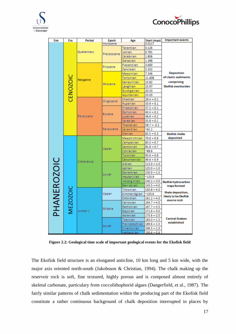
Figure 2.2: Geological time scale of important geological events for the Ekofisk field
The Ekofisk field structure is an elongated anticline, 10 km long and 5 km wide, with the
major axis oriented north-south (Jakobsson & Christian, 1994). The chalk making up the
reservoir rock is soft, fine textured, highly porous and is composed almost entirely of
skeletal carbonate, particulary from coccolithophorid algaes (Dangerfield, et al., 1987). The
fairly similar patterns of chalk sedimentation within the producing part of the Ekofisk field
constitute a rather continuous background of chalk deposition interrupted in places by

18
masses of chalk material deposited elsewhere and introduced in form of turbidities, slumps
and debris flows. The producing formations of the Ekofisk field are composed almost
exclusively of chalk with similar compositional and mechanical characteristics (Johnson, et
al., 1989).
Formations of the Ekofisk field
The Ekofisk reservoir consists of chalk from the Masstrichtian through Upper Danian Age,
Late Cretaceous to Early Paleocene epoch. The producing horizons of the Ekofisk field are
the Ekofisk and the Tor formations (Johnson, et al., 1989). The Ekofisk field is situated at a
sea depth of approximately 200 feet, and the top of the Ekofisk reservoir located at a depth
of about 9600 feet.
The Ekofisk formation is divided into three main geological layers. The Upper Ekofisk layer
is EA, followed by the middle layer, EM, and the Lower Ekofisk layer, EL. A tight non-
producible impermeable zone, represented by the layer EE, separates the Ekofisk and the
Tor formations. The underlying Tor formation is subdivided into three geological layers, the
upper layer, TA, the middle layer, TB, and the lower layer TC. The uppermost layer, TA,
forms the best quality reservoir and also contains the bulk of the reserves in the Tor
formation. The Lower Ekofisk layer, EL, is mainly composed of reworked chalk and makes
up a good reservoir rock. The upper Ekofisk is more heterogeneous with a higher degree of
impurities, mainly silica (Takla, et al., 1989), (Jakobsson, et al., 1994), (Agarwal, et al.,
1997).
The full field simulation model of the Ekofisk field is divided into 22 layers. The upper
eleven layers comprise the Ekofisk formation, the underlying three layers make up the tight
zone, and the remaining buttom eight comprise the Tor formation.
The chalk of the Ekofisk formation has a thickness ranging from 350 to 550 feet with matrix
porosities ranging from 25 to 48 %, illustrated in figure 2.3, and a low matrix permeability
of 1 to 4 millidarcies (mD). The Tor formation is slightly thinner than the Ekofisk
formation, with thickness of 350 to 500 feet with porosities ranging from 25 to 40 % and
matrix permeability similar to the Ekofisk formation. The impermeable tight zone
separating the producing part of the two formations has a thickness of 50 to 90 feet. Vertical

19
effective permeability is between 0.001 and 0.1 times that of horizontal effective
permeability and depends strongly on the presence of vertical barriers (Jakobsson, et al.,
1994). The overburden consists of approximately 9300 feet of clays and shale, which is over
pressured below approximately 4500 feet.
Figure 2.3: Formations of the Ekofisk field (Sulak, 1990)
A chalk reservoir at the depth of the Ekofisk reservoir should normally have porosities less
than 10 %. It is therefore important to understand why diagenesis of the Ekofisk and Tor
formations has retained porosities ranging from 30 % to over 40 %. There are several
possible mechanisms for retaining porosity. At this time, it is appropriate to state that
anomalously high porosity in Ekofisk field is probably due to a combination of over
pressuring of the reservoir, magnesium-rich pore fluids and early introduction of
hydrocarbons into the reservoir (Bark, et al., 1979).
Ekofisk reservoir oil
The original Ekofisk reservoir fluid was an under-saturated, moderately volatile crude oil at
initial reservoir absolute pressure of 7103 pounds per square inches (psia) and initial
reservoir temperature of 268 Fahrenheit (F) at datum depth of 10 400 ft. The initial oil had
an average density of about 850 kg/m3 and a field wide solution gas to oil ratio (GOR)
around 1530 standard cubic feet gas per standard oil barrel (SCF/STB). In 1976 the
reservoir oil went through the oil saturation pressure, which initially was 5560 psia at datum
depth 10 400 ft, resulting in gas bubbles boiling out of the reservoir oil. The field-wide
GOR being constant to this date increased to about 9000 SCF/STB by 1986 (Sulak, 1990).
Water flooding of the formations has resulted in the reservoir pressure again increasing
above the oil saturation pressure, making the oil under saturated. The current field-wide

20
GOR is approximately 1100 SCF/STB. The observed field-wide GOR history on the
Ekofisk field is illustrated in figure 2.4.
Figure 2.4: Ekofisk field-wide GOR history
Subsidence of the seafloor
The potential of compaction for high porosity chalk was recognized before the development
of the Ekofisk field. However, at that time rock mechanics and structural analysis, coupled
with case studies, led to development of certain criteria for transfer of reservoir compaction
into surface subsidence. These criteria indicated that reservoir compaction at Ekofisk should
not lead to significant subsidence (Sulak, et al., 1989). However, in November 1984
subsidence of the seafloor in the vicinity of the Ekofisk complex was discovered,
demonstrating that the initial criterias of subsidence were incorrect. The seabed under the
Ekofisk complex had subsided about 10 feet by 1984, illustrated in figure 2.5.

21
Figure 2.5: Subsidence of Ekofisk seafloor (ConocoPhillips Company(3),2012)
The subsidence is caused by compaction of the reservoir formations being transmitted to the
surface through the overburden. Reservoir compaction is caused by deformation of the chalk
matrix due increase in effective stress on the rock. The effective stress, the difference
between the overburden load on the rock and the pore pressure within the rock, increased
due to pressure depletion (Dangerfield, et al., 1987). Under initial conditions, the pore
pressure in the reservoir was about 7000 psia. The weight of 3 km thick overburden exerts a
pressure of 9000 psia, giving a net effective stress of 2000 psia. With the pore pressure
decreasing due to production, the effective stress increases resulting in compaction of the
reservoir chalk and following subsidence of the seabed (Jewhurst, et al., 1987).
The main concerns related to the subsidence were protection of the steel platforms and the
concrete storage tank. In order to buy time to come up with a solution, produced gas was re-
injected and not sold for a period. In 1986 it was decided to elevate the steel platforms and
build a concrete protective barrier around the storage tank. All platforms were elevated
within 1987 and construction of a protective barrier around the storage tank began in May
1988.
The stepwise increase of water injection in Ekofisk for the purpose of pressure maintenance
and improved oil recovery was expected to slow down or eventually stop the subsidence
rate. Despite slightly increasing reservoir pressure, subsidence continued just about 40
cm/year to 1998 (Sylte, et al., 1999). After that subsidence rates sharply declined to
approximately 10 cm/year, which have continued to present time. Figure 2.6 shows the
subsidence rate for the two platforms, Alpha and Bravo, and for the hotel complex.

22
Figure 2.6: Subsidence rate history at Ekofisk (ConocoPhillips Company(3),2012)
Fracture-matrix mechanism
The Ekofisk field has a fracture-matrix mechanism which is crucial for the reservoir being
producible. The permeability of the chalk matrix is between 1 and 4 mD. However, the
natural fractures can enhance the effective permeability a factor of 50 times the matrix
permeability in areas. The effective permeability has been calculated from well tests to be
up to 100 to 150 mD. It has been estimated that the reservoir volume represented by
fractures is less than 0.5% (Sulak, 1990).
The fractures in the Ekofisk field are of various origins and can generally be classified as
stylolite, tectonic, irregular and healed fractures. Stylolite and tectonic fractures, shown in
figure 2.7, provide enhanced permeability and are therefore of primary interest. The Ekofisk
formation is dominated by tectonic fractures, and stylolite fractures are rare. The Tor
formation is dominated by stylolite fractures, but also areas of tectonic fractures (Thomas, et
al., 1987). The tectonic fractures in the Ekofisk formation have developed parallel and
conjugate sets of fractures. The intensity of fracturing varies both vertically and areally.
Highly fractured zone have spacings as small as 5 to 15 centimeters, while zones of lower
fracture intensity have spacing of 15 to 100 centimeters. The dip of the tectonic fractures are
mainly sub-vertical with a dip varying from 60 to 80 degrees (Hallenbeck, et al., 1989). The
stylolites in the Tor formation are parallel to the beding plan and are usually only a few feet

23
apart. These fractures form permeable zones which can extend laterally for large distances
(Dangerfield, et al., 1987).
Figure 2.7: Tectonic and stylolite associated fractures (ConocoPhillips Company(3),2012)
Ekofisk drive mechanisms for oil displacement
Solution gas drive and compaction drive have been the dominant natural production
mechanisms on the Ekofisk field. Initially, solution gas drive was thought to be the
dominating drive mechanism. However, the discovery of subsidence in 1984 led to the
conclusion that compaction drive also was a dominant recovery mechanism. Water influx
into the Tor formation and oil expansion contributed to oil production the first years.
Primary depletion was also augmented by gas injection.
After concluding that water flooding was successful, it was found that the dominating
processes responsible for this was spontaneous imbibition of water into the chalk. As the

24
Ekofisk field is intensively natural fractured, the surface area subjected to imbibition is
large, contributing to water injection being effective. When production of formation water
was observed it indicated that viscous displacement was a contributing drive mechanism for
oil recovery.
Future plans
As earlier mentioned, the current plan is to continue water flooding until the production
license expires by the end of 2028. However, a wide range of EOR-mechanisms are
considered for improving the oil recovery beyond the Ekofisk water flood scenario.
Hydrocarbon WAG, carbon dioxide WAG, water chemistry and chemical flooding are
among the EOR processes assessed. Extensive laboratory experiments, reservoir simulations
and even a WAG-pilot, discussed in more detail in chapter 3, have been executed to
evaluate the incremental recovery potential. None of the EOR scenarios have yet proven to
be economically accepted to be implemented on full-field scale.

25
3 Literature review
WAG processes have been applied for more than 50 years with good success in most field
cases (Christensen, et al., 2001). The first reported WAG application took place in a
sandstone reservoir in Alberta, Canada in 1957 with a hydrocarbon miscible WAG-process.
Since that WAG applications have been applied extensively worldwide with a gradually
increase in projects, see figure 3.1. The majority of WAG injections are in onshore fields
located in Canada and United States. However, there are also several fields located in
former USSR and in the North Sea.
Figure 3.1: Cumulative number of worldwide WAG applications from the first project in 1957 to 1996
(Christensen, et al., 2001)
Purpose of WAG injection
The purpose of WAG injection is to improve oil recovery, by both increasing the
macroscopic and microscopic sweep efficiency and for pressure maintenance. The
microscopic sweep efficiency is defined by how much oil is recovered in areas contacted by
the displacing fluids. The macroscopic sweep efficiency is defined by how effective the
displacing fluids contact the reservoir in volumetric sense. In other words, how well the
displacing fluids sweep the reservoir, both vertically and areally. The main purpose of the

26
water slugs is to increase the macroscopic sweep efficiency by a more favorable
displacement mobility ratio. By a reduction of the mobility ratio larger parts of the reservoir
will be contacted and the displacing front will be more stable resulting in reduced viscous
fingering and postponed gas breakthrough to production wells. The purpose of the gas slugs
is to increase the microscopic sweep efficiency, and also contact attic oil in areas not
contacted by water injection. In high permeable sandstone reservoirs gravity segregation is
common. Gas will tend to migrate to the top of the reservoir and the more dense water will
tend to migrate to the bottom of the reservoir, hence attic oil in the upper parts of the
reservoir may be contacted by the injected gas. Usually residual oil to WAG is less than to
water or gas (SorWAG < Sorw;Sorg). Thus, a combination of the improved microscopic
displacement efficiency by gas injected with the improved macroscopic displacement
efficiency by water injection improved oil recovery can be achieved (Christensen, et al.,
2001), (Kleppe, et al., 2006).
WAG projects worldwide
Christensen et al. (2001) did a review of 59 fields where WAG injection were applied. The
review included both miscible and immiscible WAG using different types of displacing
gases, both hydrocarbon and non-hydrocarbon gases, such as carbon dioxide and nitrogen.
A common trend for the success of the reviewed fields were increased oil recovery in the
range of 5 to 10 % of the original oil in place, but increased oil recovery up to 20 % were
also reported in several fields. The average improved recovery was calculated to be 9.7%
for miscible WAG injection and as expected lower for the immiscible WAG injection at
6.4%. A positive observation from the review related to this study was that the highest
improved recovery was obtained in a carbonate formation, however it was not in offshore
environments like the Ekofisk field.
Of the 59 fields repored only six were applied in carbonate, and only six reported as WAG
injection in offshore environments. All of the six reported offshore fields were located in the
North Sea and made use of hydrocarbon gases. A typical trend for all fields were inital
WAG-ratio of 1, however some fields varied up to WAG-ratio of 4. WAG-ratio is the ratio
between volume of water and volume of gas in a WAG-cycle. The gas slug sizes reported
were generally in the range of 0.1 to 3 pore volumes, with use of low volume slug sizes
most common (Christensen, et al., 2001).

27
WAG projects in North-Sea
Kleppe et al. (2006) did a survey summerizing North Sea EOR projects in the period from
1975 to 2005. It was published that WAG injection is the most commom and successful
EOR technology for the North Sea. WAG injection have been applied in the North Sea since
1980 and is considered a mature EOR-technology. Of the 19 reviewed EOR projects in the
survery, which included both pilots and field-scale applications, nine are WAG-applications.
Of these nine WAG-applications, six are classified as immiscible-WAG, Brage and
Statfjord being field-scale WAG injections, while Ekofisk, Gullfaks, Thistle and Oseberg
Øst are WAG-pilots. Of the three miscible WAG applications only Magnus is field-scale,
while the other two at Snorre A and Brae South are WAG-pilots. In all cases hydrocarbon
gases has been used, mainly because of the availability directly from production resulting in
relativly low costs.
WAG injection in offshore environments such as in the North Sea is quite different from
onshore WAG applications. Regular injection patterns are commonly used onshore, with
five-spot injection pattern being the most common, however such patterns is typically not
used offshore. The reason for this is the high costs of drilling new wells and for data
acquisition offshore. Offshore wells are more likely to be placed based on geological
considerations (Christensen, et al., 2001), (Kleppe, et al., 2006).
CO2-WAG has also proven to be a successful EOR technology worldwide. In many cases
the method has lower minimum miscibility pressure than hydrocarbon gases which makes it
attractive. However, the high costs of CO2 capture and sequestration have so far been to
challenging for the technology to be attractive in the North Sea (Kleppe, 2006).
Previous WAG-studies at the Ekofisk field
Immiscible WAG studies for the Ekofisk field were initiated in the fall of 1993
(ConocoPhillips, January 1994). The plan was to cover a set of phases including
experimental laboratory work and reservoir modeling, which eventually could lead to the
design of a WAG-pilot and possibly further expansion to full field WAG injection (Østhus,
1998 ). Laboratory work performed included evaluation of incremental oil recovery,
compared to a water flood case, and evaluation of oil recovery mechanisms for gas
injection, following complete water imbibition into chalk samples, similar to those in the
28
Ekofisk field (Reservoir Laboratories AS, 1995). The laboratory studies substantiated WAG
potential with incremental oil recovery in the range of 20-25 %. A full field WAG screening
(ConocoPhillips, January 1994), based on optimistic assumptions, also gave good results
with the potential for WAG injection to be economically feasible. These positive results led
to the decision to proceed to pilot planning.
Ekofisk WAG-pilot
The injection well 2/4 W-06 was chosen as the WAG-injection well for the pilot. This well
was chosen due to low costs, good water injectivity being a former water injection well,
several surrounding production wells and perforations in both the Ekofisk and Tor
formations making it representative for the entire field. (Jensen, 2001), (Østhus, 1998 ). The
main objectives of this multiwell pilot was to get information on reservoir performance data
including injectivity of gas and water, sweep efficiency of injected gas in the presence of
high water saturations, timing of gas breakthrough and production response of oil, gas and
water in surronding production wells.
Gas injection in the WAG-pilot well was performed intermittenly in the period between
June 1996 and September 1996. Gas was accomodated from the nearby Charlie 2/4
production platform. The WAG-pilot was unsuccesful because substantial gas injection rates
were not achieved.
Ekofisk WAG-pilot failure and suggested solutions to hydrate formation problem
Post analysis revealed that hydrate formation in the reservoir was the reason for gas
injectivity loss. Gas hydrate formation was caused by the temperature around the former
water injection well being around F.
Labarotory experiments performed at Rogaland Research Institute (Lekvam, et al., 1997)
and at the Phillips Research Center in Barlesville (Wegener, et al., 1997) were reported
addressing and discussing several options to prevent hydrate formation, given in table 3.1,
for WAG injection in the Ekofisk Field.

29
Table 3.1: Summarize of suggested solutions to prevent the hydrate formation problem for WAG
injection at the Ekofisk field (Lekvam, et al., 1997)
Suggestions to avoid hydrate formation 1) Chemical heating of the near wellbore area prior to gas injection
2) Heating of the injection water to rise near wellbore temperature prior to gas injection
3) Sidetrack the injectors outside cooled zones prior to gas injection
4) Co-injection of water and gas
5) Chemical inhibition to prevent and/or retard the onset of hydrate formation
The reports (Wegener, et al., 1996), (Lekvam, et al., 1997) concluded that co-injection of
water and gas would not be a solution in itself, but would be required to achieve necessary
bottom-hole pressure (BHP), above the reservoir pressures. Further the reports concluded
that chemical inhibition would not be capable of avoiding the hydrate formation. Increasing
the near wellbore temperature, by chemical heating or by injecting heated water prior to gas
injection was neither found to be solutions. A model showed that the injected gas would
move much faster than the heating water front and eventually move ahead of the heating
front, leading to hydrate formation. Similarly chemical heating might raise temperature near
the wellbore. However, the cold zone is pushed ahead into the reservoir and will be reached
when injecting gas. The only remaining option was to sidetrack the injection wells outside
the cool temperature regions. Sidetracking the injection wells outside the cooled region still
means that the injected water temperature needs to be above hydrate formation temperature,
and a sufficiently high BHP is needed to overcome the high reservoir pressure. Some
unsuccessful attempts were performed to prevent hydrate formation, and the WAG well was
eventually changed back to a water injection well (Østhus, 1998 ).
Ekofisk WAG-studies in the posterity of the WAG-pilot
Full field WAG simulations indicated incremental oil recovery potential up to 6 %, above a
Ekofisk water flood case from 1997 (Østhus, 1998 ). The potential oil production for a full
field WAG-simulation, with field gas injection rates of 600 million standard cubic feet per
day (SCF/D), was compared to a long term water flood production forecast, from 1997 until
end of license in 2028, and is shown in figure 3.2.

30
Figure 3.2: Full field WAG-simulation versus long term water flood production forecast (Østhus, 1998 )
Some of the assumptions made in the full field simulation model were good gas injectivity,
no relative permeability hysteresis effect and low trapped gas saturation. Further
assumptions were that injected gas would contact residual oil in the matrix block, either by
forced displacement and/or by diffusion mechanisms, and eventually vaporize parts of the
residual oil after the water flooding (Østhus, 1998 ). The displacement process was assumed
immiscible, with the injected gas composition used given in table 3.2.
Table 3.2: Composition of injected gas used in previous Ekofisk WAG-simulations (Østhus, 1998 )
Component Mole (%)
Nitrogen, N2 0.4
Methane, C1 85.4
Carbon dioxide, CO2 2.1
Ethane, C2 8.1
Propane, C3 2.8
2-Metylpropan, i-C4 0.3
n-Butane, n-C4 0.9

31
A major EOR screening study (Harpole, et al., 2000) was performed in 1998-1999 where
HC-WAG was reported among the top two processes to be carried forward in further
studies. The screening study recommended to update full field WAG development forecasts,
with progression towards a new pilot if full field economics were sufficient.
Further WAG studies re-evaluating full field WAG potential were performed in 2000-2001
(Jensen, 2001). A premise for the study was that any unresolved technical or logistical
issues had to be successfully addressed or solved prior to further process implementation.
Based on the premise the study concluded with WAG not being technically or economically
viable at this point.

32
4 Theory
This chapter is initiated with description of general reservoir and fluid parameters which
affect reservoir simulations and the main parameters and concepts of this study. Next,
presentation of definitions, correlations and models regarding the main parameters and
concepts of this thesis, such as trapped gas saturation, relative permeability hysteresis and
SORM are given.
Oil recovery mechanisms for WAG-displacement, divided into oil displacement by gas and
oil displacement by water are then presented. The subsequent section presents difference
between miscible and immiscible WAG-injection, and how to evaluate miscibility through
tests on minimum miscibility pressure and minimum miscibility enrichment. The last part of
the chapter is an introduction to the full field numerical simulation tool, PSim, which is used
for reservoir modeling in this thesis.
4.1 Rock properties
4.1.1 Porosity
Porosity (φ) of a porous rock is the fraction of the total rock volume that is occupied by void
space. The porosity describes the fluid storage capacity of the rock.
4.1.2 Absolute permeability
Permeability (k) of a rock is associated with the rock’s capacity to transport fluids through
systems of interconnected pores. Permeability is a measure of the fluid conductivity of a
particular rock, in terms of Darcy (Ursin, et al., 1997).
Absolute permeability of a porous medium refers to the permeability when saturated with a
single fluid. The rock property, absolute permeability, is constant for a particular porous
medium and is independent of the fluid type flowing in the rock.

33
4.1.3 Effective permeability
In cases of multi-phase flow, when several fluids or phases are flowing locally and
simultaneously in a system, each fluid phase will counteract the free flow of the other
phases and a reduced phase permeability of each phase is measured, called the effective
permeability (Ursin, et al., 1997). Effective permeability (ke) is a measure of the fluid
conductance of one particular fluid, when that fluid fills a fraction of the pore space of a
porous medium.
4.2 Relative permeability
Relative permeability (kr) is a property used to describe flow in a multi-phase system. The
property is a fluid-rock property and is defined as the ratio of the effective permeability of a
particular fluid at a particular saturation to a base permeability of the porous medium, as
given in equation 4.1. The base permeability is usually referred to the absolute permeability
of the porous medium.
Equation 4.1
Relative permeability is dimensionless and has values between 0 and 1. If a single fluid is
present in a rock, the effective permeability will be equal to the absolute permeability; hence
the relative permeability will be equal to one. If the relative permeability of a fluid is zero,
the fluid will be immobile.
Relative permeability is mainly a function of fluid saturations and saturation history.
Dependence on saturation history is described as relative permeability hysteresis effect.
Water relative permeability depends most strongly on its own phase-saturation and typically
shows little hysteresis effect. The non-wetting phase relative permeability though depends
strongly on both the saturation of its own phase and on the saturation history. This results in
a complex saturation pattern which demands special relative permeability description,
illustrated in figure 4.1. Relative permeability hysteresis is important in WAG-processes
because the alteration between water and gas injection results in changes of saturation,
between imbibition and drainage processes, which can result gas getting trapped and
consequently change in relative permeability curves. Drainage is referred to as a process

34
where the wetting-phase saturation decreases and contrary imbibition to a process where the
wetting-phase saturation increases. A more detailed discussion on trapped gas and hysteresis
effected relative permeability curves will be given in chapter 4.6.
Figure 4.1: Example of hysteresis affected gas relative permeability imbibition curve
4.2.1 Two-phase relative permeability
Two-phase flow refers to a process where only two fluids or phases are flowing locally and
simultaneously in a system. Relative permeability of water (krw) and oil (krow) in a water-oil
system are plotted in relative permeability curves as a function of the water saturation.
Similarly, the relative permeability of gas (krg) and oil (krog) in a gas-oil system are plotted
in relative permeability curves as a function of the gas saturation. Figure 4.2 (a) and (b)
illustrates typical shape of two-phase relative permeability curves for water-oil and gas-oil
systems respectively.
Relative permeability curves allow comparison of fluid flow at different fluid saturation and
estimation of residual oil and gas saturations based on endpoint saturations. Endpoint
saturations are reflected by the largest saturation of a phase for which the relative
0
0,005
0,01
0,015
0,02
0,025
0,03
0,035
0,04
0 0,05 0,1 0,15 0,2 0,25 0,3
Krg
Sg
Drainage
Imbibition

35
permeability of the respective phase in the respective system is zero. Endpoint saturations in
a water-oil system are defined Sorw for oil and Swr for water, figure 4.2 (a). Similarly, for a
gas-oil system the endpoint saturations are defined as Sorg for oil and Sgr for gas, figure 4.2
(b). If the saturation of a coexisting phase becomes less than the endpoint saturation, the
relative permeability will be zero and the phase immobile. Endpoint saturations are also of
great importance for estimation of initial fluid distribution and ultimate recovery of systems.
(a) (b)
Figure 4.2: Illustration of the shape of (a) water-oil relative permeability curves, and corresponding
end-point saturations (b) gas-oil relative permeability curves, and corresponding end-point saturations
Even though there have been attempts to calculate relative permeability on theoretical
backgrounds, most work is done experimentally. The experimental work on relative
permeability is mostly performed on the two-phase systems water-oil and gas-oil.
Relative permeability data can be obtained experimentally by centrifuge techniques or by
core flooding tests under steady-state or unsteady-state conditions. In unsteady-state relative
permeability tests, cores with in-situ fluid are flooded with an immiscible fluid, gas or
water, at constant rate. Values for relative permeability are determined using a Buckley and
Leverett developed equation based on observations of the fractional flow of the displacing
fluid phase, which are related to saturation. In steady-state tests two fluids are injected
simultaneous in a core at constant rate until the produced fluid ratio comes in equilibrium
with the injected fluid ratio. Phase saturations are measured and the corresponding relative
permeability is obtained by applying Darcy’s law. Relative permeability for different

36
saturations can be obtained by changing the fluid ratio of the injected fluids (Ibrahim, et al.,
2001). In centrifuge tests a liquid saturated sample is placed in an air-filled core holder and
subsequently rotated with constant speed in a centrifuge. Relative permeability values are
obtained by monitoring the liquid production as a function of time at a given rotational
speed (Spronsen, 1982) (Firoozabadi, et al., 1986).
The centrifuge method is relative fast; however it has been limited to determination of
wetting-phase relative permeability only (App, et al., 2002). Unsteady-state tests have
shown to yield faster results than steady-state tests. Steady-state tests have though been
preferred for reservoir with more-scale heterogeneity and with mixed wettability (Ursin, et
al., 1997), (Ibrahim, et al., 2001).
In lack of reliable two-phase relative permeability data, simplified models based on
experimental data can be used to construct two-phase data. An example of such a model is
the Corey-type approximations which uses a power law function to calculate relative
permeability based on endpoint saturations and empirical parameters.
4.2.2 Three-phase relative permeability
Locally in reservoirs three phases can flow simultaneously. To describe such three-phase
flow, three-phase relative permeability data is required. For WAG-displacement, local three-
phase flow is common, and is especially evident close to injectors, see figure 4.3. In a three-
phase system there will be an intermediate wetting-phase in addition to the phases present in
two-phase systems. In a water-wet system, oil will be the intermediate wetting-phase and act
as a non-wetting phase with respect to water and as a wetting-phase with respect to gas.
Figure 4.3: Three-phase flow in a WAG-system (Skauge, et al., 2007)

37
Estimates of three-phase relative permeability are needed to understand three-phase flow.
As most experimental data on relative permeability are on two-phase systems, a number of
correlations and models to calculate three-phase permeability have been developed.
However, there is little experimental data to validate most models (ConocoPhillips
Technical Manual, 2010). The most accepted and commonly used three-phase relative
permeability models in the petroleum industry are the two proposed by Stone.
4.2.2.1 Stone’s models
Stone’s models (Stone 1970, 1973) are probability-based models which assume the relative
permeability of the wetting and non-wetting phases depend only on the saturation of the
wetting and non-wetting phases respectively, while the intermediate wetting-phase relative
permeability varies in a more complex manner. For a water-wet system, water will be the
wetting phase, gas the non-wetting phase and oil the intermediate wetting-phase.
Stone’s models use more easily measured two-phase data, water-oil and gas-oil relative
permeability curves, to predict the relative permeability of the intermediate-wetting phase in
a three-phase system.
In many reservoirs that involve three-phase flow only gas and oil are mobile in the upper
parts, and only water and oil are mobile in the lower parts, as illustrated in figure 4.3.
Stone’s models therefore predict that the oil relative permeability, kro, is obtained as
function of oil relative permeability from the water-oil system (krow) in presence of water
only, and as a function of oil relative permeability from the gas-oil system (krog) in presence
of gas and irreducible water.
In areas of three mobile phases the technique used to obtain three-phase relative
permeability for the intermediate wetting-phase is to interpolate between the two sets of
two-phase relative permeability data, using krw, krow, krg and krog, krw and krow are obtained
from the water-oil data as function of water saturation. Similarly, krg and krog are obtained
from the gas-oil data as a function of gas saturation holding the water saturation constant
and immobile. Hence, the two-phase relative permeability curves for water-oil and gas-oil
are sufficient for use of Stone’s models.
Both Stone’s models have the desirable property in that they yield the correct two-phase
data when only two phases are flowing, and yet provide interpolated data for three-phase

38
flow that are consistent and continuous functions of the phase saturations. To allow for
hysteresis effect, the water and gas saturations should be changing in the same direction in
the two sets of two-phase data, as desired in the three-phase system.
4.3 Surface and interfacial tension
Whenever immiscible phases coexist in a porous medium, surface energy related to the fluid
interfaces influences the saturations, distributions and displacement of the phases (Green, et
al., 1998). The surface force between two fluids is quantified in terms of surface/interfacial
tension, σ, which is given as the force acting in the plane of the surface, per unit length of
the surface.
Surface tension is usually reserved to the case when the interface is between a liquid and its
vapor or air. If the interface is between two different fluids or between a liquid and a solid,
the term “interfacial tension” (IFT) is used.
4.4 Rock wettability
Wettability can be defined as the tendency of one fluid to spread or to adhere to a solid
surface in the presence of a second fluid. (Ursin, et al., 1997) When two immiscible phases
are placed in contact with a solid surface, one phase usually is attracted to the solid more
strongly than the other phase. The more strongly attracted phase is called the wetting phase
(Green, et al., 1998).
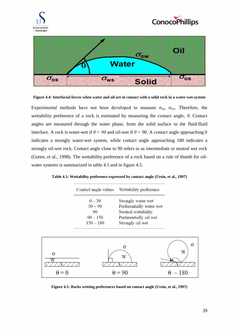
Quantitative evaluation of wettability can be done by examining the interfacial forces that
exist when two immiscible fluid phases are in contact with a solid. In figure 4.4, forces
between the solid, water and oil are balanced and given by:
Equation 4.2
Where σos, σws and σow are interfacial tensions between solid and oil, water and solid and
water and oil respectively, and θ is the contact angle measured through the water.
39
Figure 4.4: Interfacial forces when water and oil are in contact with a solid rock in a water-wet-system
Experimental methods have not been developed to measure σos, σws. Therefore, the
wettability preference of a rock is estimated by measuring the contact angle, θ. Contact
angles are measured through the water phase, from the solid surface to the fluid-fluid
interface. A rock is water-wet if θ < 90 and oil-wet if θ > 90. A contact angle approaching 0
indicates a strongly water-wet system, while contact angle approaching 180 indicates a
strongly oil-wet rock. Contact angle close to 90 refers to as intermediate or neutral wet rock
(Green, et al., 1998). The wettability preference of a rock based on a rule of thumb for oil-
water systems is summarized in table 4.1 and in figure 4.5.
Table 4.1: Wettability preference expressed by contact angle (Ursin, et al., 1997)
Figure 4.5: Rocks wetting preferences based on contact angle (Ursin, et al., 1997)

40
The state of rock wettability will affect the distribution of fluids within a reservoir system,
see figure 4.6.
Figure 4.6 Fluid distributions within water-wet and oil-wet systems (Green, et al., 1998)
Rock wettability will also affect relative permeability-, illustrated in figure 4.7, and capillary
pressure characteristics of a fluid-rock system, which is likely to result result in differences
in residual oil saturations (Green, et al., 1998), (Donaldson, et al., 1969).
Figure 4.7: Wettability effect on relative permeability curves for (a) water-wet systems and (b) oil-wet
systems (Ursin, et al., 1997)

41
In water-oil systems, oil will be more mobile, and lower water flood residual oil saturations
will be exhibit than in an oil-wet system. Likewise, water will flow better in oil-wet systems
and higher water flood residual oil saturation will be left in the reservoir.
Strongly water-wet system will spontaneously imbibe more water into the matrix blocks
than a preferentially water-wet system. Spontaneous imbibition of water into matrix blocks
is important for oil recovery and is described in more detail in chapter 4.9.1.2.
4.5 Capillary pressure
A pressure difference called capillary pressure will exists across the interface between
immiscible fluids caused by interfacial tensions. Capillary pressure, Pc, is defined as the
pressure difference between the non-wetting phase, Pnw, and the wetting-phase, Pw, given by
equation 4.3 (Ursin, et al., 1997):
Equation 4.3
Young-Laplace presented a relationship between the capillary pressure and the interfacial
tension between two immiscible fluids on a curved surface, given in equation 4.4, with
examples of radius of curvature shown in figure 4.8:
Equation 4.4
Figure 4.8: Radius of curvature on a curved surface (Ursin, et al., 1997)
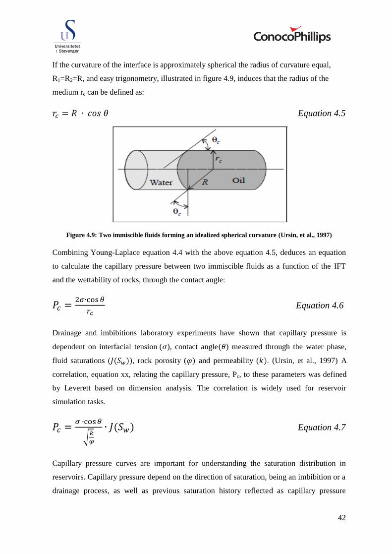
42
If the curvature of the interface is approximately spherical the radius of curvature equal,
R1=R2=R, and easy trigonometry, illustrated in figure 4.9, induces that the radius of the
medium rc can be defined as:
Equation 4.5
Figure 4.9: Two immiscible fluids forming an idealized spherical curvature (Ursin, et al., 1997)
Combining Young-Laplace equation 4.4 with the above equation 4.5, deduces an equation
to calculate the capillary pressure between two immiscible fluids as a function of the IFT
and the wettability of rocks, through the contact angle:
Equation 4.6
Drainage and imbibitions laboratory experiments have shown that capillary pressure is
dependent on interfacial tension ), contact angle ) measured through the water phase,
fluid saturations ( , rock porosity ( and permeability ( . (Ursin, et al., 1997) A
correlation, equation xx, relating the capillary pressure, Pc, to these parameters was defined
by Leverett based on dimension analysis. The correlation is widely used for reservoir
simulation tasks.
Equation 4.7
Capillary pressure curves are important for understanding the saturation distribution in
reservoirs. Capillary pressure depend on the direction of saturation, being an imbibition or a
drainage process, as well as previous saturation history reflected as capillary pressure

43
hysteresis effect. Common shape of water-oil capillary pressure curves for drainage and
imbibition processes are shown in figure 4.10:
Figure 4.10: Illustration of water-oil capillary pressure curves
The capillary pressure, created as a result of interactions between liquids and solid surface,
is responsible for the spontaneous imbibitions of water into the matrix blocks. Water will
spontaneous imbibe the matrix block until the capillary pressure equals zero.
In case of three-phase flow, three-phase capillary pressures curves are needed to model the
dynamics of gas-oil and oil-water transition zone movements in the reservoir (Helland, et
al., 2004). There has been little experimental work done on three-phase capillary pressure
(Skauge, et al., 2007). Three-phase capillary pressure curves have traditionally been
estimated from experimentally measured two-phase capillary pressure data. However,
experimental work on three-phase capillary pressure reported by Bradford and Leij (1995)
indicated that this practice may not be valid. Although experimental data is very limited
there exist a few correlations to calculate three-phase capillary pressure. Helland and
Skjævland (2004) presented a three-phase capillary pressure correlation accounting for
direction of saturation change as well as wettability conditions. They validated the
correlation with centrifuge measurements from water-wet cores. The correlation have not
yet been widely accepted or validated, and capillary pressures are often neglected in three-
phase flow processes like WAG-injection.
44
4.6 Trapped gas saturation and hysteresis effect
4.6.1 Introduction to trapped gas saturation and hysteresis
Phase trapping of gas is a common phenomenon after an imbibition process where a
wetting-phase displaces the non-wetting phase gas (Green, et al., 1998). Trapped gas is
important in WAG processes, because the WAG cycles lead to oscillation of water and gas
with position and time (Skauge, et al., 2007), which induce changes between drainage and
imbibition processes.
For water-wet systems gas is always the non-wetting phase, and invades the larger pores and
throats (Suicmez, et al., 2006). During the imbibition process the capillary pressure in the
larger pores is less than the capillary pressure in the smaller pores. As a consequent, the
wetting phase will advance faster in the smaller pores and part of the gas phase will be
bypassed by the increasing wetting phase. This disconnection of the former continuous gas
clusters will leave a portion of the gas phase immobile and trapped as isolated drops or
ganglia. The isolated gas will be held in the larger pores by strong capillary forces which
cannot overcome the relative small viscous forces (Green, et al., 1998). As the trapped,
immobile part of the gas saturation does not contribute to flow of gas, the gas relative
permeability at a given gas saturation will be less for the imbibition process compared to the
drainage process. The change of imbibition relative permeability curves compared to
drainage curves is called relative permeability hysteresis effect and is mainly caused by the
trapped gas. Different models and correlations accounting for hysteresis effect relative
permeability curves and for modeling trapped gas saturation will be presented in this section.
Several studies have been performed on determining the parameters that impact the amount
of gas getting trapped. Trapped gas saturations have been reported (Suicmez, et al., 2006),
(Wegener, et al., 1996) function of on pore geometry and porosity and the saturation history,
both current and historical maximum gas saturation. Laboratory experiments on carbonate
cores by Keelan and Pugh (1975) indicated that trapped gas is independent of pore geometry
and porosity for chalk formation. Further their experiments confirmed that increasing gas
saturation is accompanied with increasing trapped gas saturation. Pow et al. (1997)
addressed imbibition of water in fractured reservoirs. Field and laboratory information
suggested that a large amount of gas was trapped by fast water imbibition through the
fractures.

45
Several correlations have been proposed in the literature to calculate the amount of trapped
gas saturation. The most accepted is the one proposed by Carlson S. Land. Land’s
correlation is the correlation commonly used in hysteresis models to calculate the amount of
trapped gas.
4.6.2 Trapped gas saturation correlations and hysteresis models in PSim
4.6.2.1 Land’s correlation
Land’s trapped gas
Carlson S. Land addressed an empirical correlation (Land, 1968), (Land, 1971) based on
available data which relates initial gas saturation at the start of an imbibition process to the
trapped gas saturation at complete imbibition:
Equation 4.8
Where:
: Residual (trapped) gas saturation after complete imbibition1
: Gas saturation established in the drainage process and the initial gas saturation
of the imbibition process
CLand : Trapping characteristic of the porous rock called Lands constant
The trapping characteristic of the porous rock, Lands constant, is determined by:
Equation 4.9
Where:
: Maximum obtainable residual gas saturation, corresponding to initial gas
saturation at one minus critical water saturation.
1 All saturation marked with stars are effective saturation expressed as fraction of the pore
volume excluding the pore volume occupied by the irreducible wetting phase.

46
Land’s relative permeability hysteresis effect
Land further proposed that only the mobile part of the gas-phase should be used to calculate
hysteresis affected relative permeability imbibition curves. The total gas saturation, , at
any point in the imbibition process can be treated as two separate saturations, a mobile
fraction of the gas, , and the current trapped gas fraction of the gas, :
Equation 4.10
If a total saturation, is reduced to a residual trapped gas saturation, the
contribution from the mobile fraction, to residual trapped gas saturation can be found
by applying SgF* as an initial saturation in equation 4.8. The gas saturation that gets
trapped, contribution of SgF*, during a reduction in gas saturation from Sg* to Sgr*, must
equal the residual value Sgr* associated with Sgi*. From this deduction, the current trapped
gas saturation can be expressed as:
Equation 4.11
Substituting equation 4.10 into equation 4.11 and solving for SgF* deduce the remaining
mobile gas saturation when the gas saturation has been reduced from Sgi* to Sg* in an
imbibition process:
Equation 4.12
Based on the mobile gas saturation SgF* calculated from equation 4.12, Land proposed that
new hysteresis effected gas relative permeability data can be calculated by using equation
4.13:
Equation 4.13
Where:
: Empirically determined pore-size distribution factor
47
4.6.2.2 Coats correlation
Coats proposed a linear correlation relating the initial gas saturation at the start of an
imbibition process to trapped gas saturation at complete imbibition (ConocoPhillips
Technical Manual, 2010):
Equation 4.14
Where:
: Critical gas saturation
C : Trapping characteristic of the porous rock given by:
Equation 4.15
4.6.3 Other relative permeability hysteresis models
A number of hysteresis empirical models have been developed to characterize the hysteresis
effect on relative permeability (Spiteri, et al., 2004).The most important parameter
determining the significance of hysteresis effect is the trapped non-wetting phase saturation.
Relative permeability models that incorporate with hysteresis are usually based on the
trapping model proposed by Land in the previous section.
Two-phase hysteresis models have been the standard in most reservoir simulators. The most
popular are described by Carlson and Killough (Larsen, et al., 1998). Standard two-phase
hysteresis models for non-wetting phase consist of one drainage relative permeability curve
and one imbibitions curve connected at the same inflection point. An inflection point is the
point where the displacement process shifts from drainage to imbibition (Larsen, et al.,
1995). The drainage-imbibition curves form a reversible envelope in which scanning-curves
are generated (Skauge, et al., 2007). The standard hysteresis models for the non-wetting
phase allows for reduced mobility in the imbibition curve after primary drainage. However,
further drainage-imbibition processes are described within the primary drainage-imbibition
envelope, where scanning curves are used to represent any subsequent drainage process.
Experimental observations have indicated that the two-phase hysteresis models do not
sufficiently describe WAG processes (Skauge, et al., 1994). Experimental observations
have shown that the mobility during secondary drainage generally is considerably lower

48
than during primary drainage. This indicates that the reversibility within two-phase models
is inappropriate. Larsen and Skauge therefore developed a three-phase hysteresis model that
includes impact further changes in trapped gas saturation have on mobility and following on
relative permeability curves.
4.6.3.1 Carlson hysteresis model
Carlson hysteresis model describes hysteresis effect of the relative permeability curves
using an experimental primary drainage curve together with an estimated imbibition curve
based on Land’s trapped gas correlation (Carlson, 1981). Further saturation changes,
between drainage and imbibition, are produced by scanning curves parallel to the estimated
imbibition curve. The imbibition curve is simply shifted until it intersects with the drainage
curve for the relevant saturation for saturation direction change, illustrated in figure 4.11
(Kossack, 2000).
Figure 4.11: Carlson hysteresis affected non-wetting phase relative permeability curves (Kossack, 2000)
The outer lines in figure 4.11 represent a primary drainage curve connected with an
imbibition curve, which is estimated based on the largest possible non-wetting phase. These
curves make up a relative permeability envelope where scanning-curves are generated
(Larsen, et al., 1995). Whenever a drainage process ends, a subsequent imbibition will
follow a scanning-curve. After initiating an imbibition process all further processes are
assumed reversible; the scanning-curve is followed back to the inflection point and the
primary drainage curve is followed to a new historical maximum of gas saturation. If the

49
drainage process stops on the scanning-curve, imbibition is computed along the same
scanning-curve.
4.6.3.2 Killough hysteresis model
Killough hysteresis model is similar to Carlson’s model founded on Land’s trapped gas
correlation (Larsen, et al., 1995) ,(Killough, 1976). The only experimental data needed in
this model is the bounding primary drainage curve, and data to estimate the bounding
imbibition curve based on Land’s correlation. The bounding drainage-imbibition curves
make a reversible envelope, where scanning curves are estimated, illustrated in figure 4.12,
based on the drainage curve through an interpolation method using a parametric curve or a
normalized experimental imbibition relative permeability relation. The hysteresis model
predicts the bounding imbibition relative permeability curve by first calculating the amount
of non-wetting phase that will be trapped by Land’s correlation, and then interpolate
between the relative permeability at the historical maximum gas saturation and zero relative
permeability at the trapped gas saturation.
Figure 4.12: Killough hysteresis affected non-wetting phase relative permeability curves (Killough,
1976)
Subsequent to an imbibition process the drainage curve will follow the scanning curve till
the maximum historical non-wetting phase has been reached, then continue along the
primary drainage curve.
4.6.3.3 Skauge and Larsen three-phase hysteresis model
The hysteresis model of Skauge and Larsen is often referred to as the WAG-hysteresis
model and is based on Carlson’s hysteresis model and Land’s trapped gas correlation
(Kossack, 2000). The model contains two Carlson hysteresis envelopes, one for high

50
mobility and one for low mobility, illustrated in figure 4.13. Each of the envelopes obeys
the rules of Carlson model in which scanning curves are produced parallel to the imbibition
curves.
Change between the envelopes is activated when gas saturation increases in a drainage
process, following the primary drainage-imbibition cycle (Larsen, et al., 1995). In
simulation of WAG processes small saturation changes caused by stability problems occur
frequently. To prevent these saturation oscillations to change between envelopes, the model
was modified by introducing a saturation tolerance limit. This limit must be exceeded before
a change between envelopes take place.
Figure 4.13: Skauge and Larsen hysteresis affected gas relative permeability curves, changing between a
high and a low mobility envelope. (Larsen, et al., 1995)
The model can also define different water relative permeability curves within each envelop,
illustrated in figure 4.14. Two different water relative permeability curves can be given as
input, and a change between the curves occur corresponding to change in gas-phase
envelops.

51
Figure 4.14: Skauge and Larsen water relative permeability curves, changing between a high mobility
curve and a low mobility curve in correspondence with the gas-phase envelops in figure 4.13. (Larsen, et
al., 1995)
4.7 Miscible flood residual oil saturation (SORM)
The residual oil left behind in the reservoir after a miscible WAG-process, the miscible
flood residual oil saturation, is important to include in field-scale reservoir simulations to
correctly evaluate the oil recovery. Compositional reservoir simulators may entirely sweep
grid blocks in miscible flooding or close to miscible flooding, which will give an optimistic
prediction of the oil recovery (ConocoPhillips Technical Manual, 2010). Complete oil
sweep is unlikely to be achieved in field-scale even under perfect miscible conditions with
first contact miscibility. There are several reasons for this, such as bypassed oil because of
heterogeneities as fractures, capillary trapping of oil, viscous fingering and heavy
component precipitations as asphaltenes and wax. The assumption of total mixing of all
hydrocarbons within grid blocks is the reason for simulation to over predict oil recovery.
The equation of state (EOS) in the simulator may allow all oil components to vaporize into
the gas phase leading to oil saturations below user-defined Sorg and Sorw.
Various techniques have been proposed to account for SORM. Some of the techniques are:
1) To introduce an artifact heavy component so that, under reservoir conditions, the heavy
component will not vaporize into the gas phase. This technique has not been recommended
because it may completely miss fluid properties such as the density and viscosity.

52
2) Treat the miscible residual oil as a part of the rock. A user-defined SORM value can be
defined as part of the rock such that oil saturation will not decrease beyond the SORM
value. The excluded oil cannot contribute to rock wettability and to solution gas if the
pressure falls below the bubble point.
3) Modification of the compositions of oil and gas phases that are flowing into or out of a
grid block by an alpha factor method. A drawback of this technique is that there are too
many parameters to tune per grid block, and the imposed SORM cannot be exactly honored.
4) The default method implemented in PSim is that a specified volume of the initial oil in
place corresponding to SORM will be isolated and considered as a fourth phase in a
different medium. A modified three-phase compositional model is used, which includes
Sorm as a part of the oil saturation together with the mobile oil saturation, Som.
Equation 4.16
Various options can be used to account for wettability effect, and mass exchange via
vaporization and condensation between the isolated oil and the flowing hydrocarbons.
5) Another technique available in PSim for SORM, is for SORM to only take effect
internally for a grid block when the oil saturation in the grid becomes less than or equal to a
defined SORM. This way SORM will not impact the flow as long as the oil saturation is
larger than the defined SORM in the grid blocks. The check for a triggered SORM is done
for each grid block at the end of the time steps (ConocoPhillips Technical Manual, 2010).
4.8 Matrix-fracture mechanisms
In the Ekofisk reservoir most of the fluid is stored in the matrix blocks, however without the
fractures the Ekofisk field would likely not be producible. Even though the fractures only
comprise about 0.5 % of the total reservoir volume they can enhance the effective
permeability from 1 to 4 mD up to 100 to 150 mD, which enables fluid flow towards the
production wells.
The primary method for detecting the fractures on the Ekofisk field is through well testing
(Dangerfield, et al., 1987). Matrix permeability, kmat, derived from well log porosity and

53
core permeability correlations are compared with the measured effective permeability from
well tests, kwell, and a fracture intensity factor, FI, can be deduced:
Equation 4.17
Different regions of the Ekofisk fields have different type of fractures, which makes up
different kind of fracture-networks. The distribution of fracture types, fracture width,
fracture lengths and fracture intensity factors, is not uniform throughout the reservoir.
Therefore different matrix-fracture models representing different regions of the reservoir
will be designed in this thesis.
The traditional yet efficient and effective approach to model naturally fractured reservoirs
has been through dual porosity models (Heeremans, et al., 2006). In dual porosity models
the fracture and matrix systems are separated into different continua with its own sets of
properties.
When reservoirs with fracture systems are depleted, initially fluid will only be produced
from the fractures (Dangerfield, et al., 1987). Because the fractures only comprise about 0.5
% of the reservoir volume, they are quickly depleted. As the fractures are depleted, a
pressure difference between matrix blocks and fractures will develop. The pressure
difference will lead to matrix blocks starting to feed fluid to the fracture system. Eventually,
the production rate will be determined by the fluid influx rate from the matrix into the
fractures. The fractures will then only enhance the net flow capabilities of the chalk matrix.
The mass transfer between matrix blocks and fractures is in dual porosity models modeled
through a transfer function, which is the heart of the dual porosity models as it controls the
matrix-fracture interaction and production performance of naturally fractured reservoirs
(Heeremans, et al., 2006) (Warren, et al., 1963).
At this time dual porosity models are not available in PSim, instead a single porosity/single
permeability model is used to describe matrix-fracture systems in full field simulations
where matrix and fractures are modeled within the same grid blocks with a shared set of
properties.
54
4.9 Recovery mechanisms relevant to WAG
The oil left in the reservoir after water flooding comprises both bypassed oil in unswept
reservoir zones and residual oil in water swept zones. Bypassed oil is associated with poor
macroscopic sweep efficiency, while the residual oil in water swept zones is associated with
poor microscopic sweep efficiency. WAG-injection is implemented to improve microscopic
sweep efficiency compared to water injection because of gas half-cycles, and to improve
macroscopic sweep efficiency compared to gas injection because of water half-cycles.
In this section WAG recovery mechanisms, displacement of oil by gas and by water, will be
presented.
4.9.1 Oil recovery mechanisms for water injection
The most important forces acting to recover oil from water injection are viscous forces,
gravity forces and capillary forces (Morrow, 1979).
4.9.1.1 Gravitational displacement
Displacement of oil in a fractured system by gravitational forces is the mechanism where
water forces into the matrix blocks due to difference in fluid densities.
Gravitational forces might arise because of different water-oil contact in the fracture system
and the matrix blocks. Difference in fluid densities give rise to a pressure difference and a
gravity potential for water to be forced into the matrix blocks. The gravity potential, , is a
given by:
Equation 4.18
Where:
: Fractional height of water in the fracture
: Fractional height of the gas in the matrix
: Water density
: Oil density
: Gravitational constant
: Height of matrix blocks

55
In the case of the Ekofisk field, matrix blocks heights are estimated in the range of one to
three feet, and the gravity potential between water and oil is normally negligible compared
to capillary and viscous forces.
4.9.1.2 Capillary displacement - spontaneous imbibition
Spontaneous imbibition is the mechanism where one fluid displaces another from a porous
medium as a result of capillary forces only. The matrix is a porous medium with a capillary
pressure, and the fractures have approximately zero capillary pressure (Heeremans, et al.,
2006). This results in a capillary pressure potential which allows the water to flow into the
matrix to release oil.
Spontaneous imbibition has been widely studied because of its importance on oil recovery,
with much emphasis on carbonate rocks. In fractured reservoirs, spontaneous imbibition of
water due to strong capillary forces is regarded as an important and necessary mechanism to
attain high displacement efficiency
The rate of imbibition is primarily dependent on the rock permeability, pore structure, rock
wettability, and the interfacial tension between fluids. Oil recovery due to spontaneous
imbibition can be determined from the capillary imbibition pressure curve. The higher water
saturation value for capillary pressure equals to zero, the better is the spontaneous
imbibition. The limit of spontaneous imbibition is determined where the imbibition capillary
pressure curve equals to zero. The degree of spontaneous imbibition is a function of
wettability as illustrated in figure 4.15. For more water-wet system higher water saturation
can be achieved for capillary pressure equals to zero, hence better water imbibition into
matrix blocks.

56
Figure 4.15: Capillary imbibition as a function of wettability
Further forced imbibition of water into matrix blocks at negative capillary pressures requires
external forces like viscous or gravitational forces. In fractures reservoir where both
spontaneous imbibition and viscous displacement is evident, the residual oil saturation after
water flooding will depend more on the shape of the negative part, forced imbibition, of the
capillary pressure curve and the magnitude of pressure drop than on the spontaneous
imbibition part.
4.9.1.3 Viscous displacement
Viscous displacement is the mechanism where water is forced from the fracture system into
matrix blocks due to a pressure gradient over the matrix blocks. Pressure differences in the
reservoir results due to production, extracting fluids and decreasing the pressure, and
injection, adding fluids and increasing the pressure.
The external pressure drop, over the matrix blocks, will force water into the matrix blocks
until a balance between the viscous forces and capillary forces are reached. In the case of
the Ekofisk field the pressure drop over matrix blocks is about 1 psi/ft.
4.9.2 Oil recovery mechanisms for gas injection
The most important oil recovery mechanisms for gas injection into a fractured reservoir are
condensation of gas into oil, vaporization of oil, gravity drainage, diffusion and viscous
displacement (Jakobsson, et al., 1994). Viscous displacement, gravity drainage and diffusion

57
are mechanisms for gas to enter the matrix blocks, while condensation and vaporization are
the mechanisms for oil to expel into the fractures to be produced. The mechanism of viscous
displacement for gas is such as described for water and will not be presented.
4.9.2.1 Vaporizing gas drive / oil stripping
Vaporizing gas drive is the mechanism where low molecular-weight hydrocarbons, ethane
to heptanes, vaporize from the reservoir oil (Holm, 1987). As injected gas enters the matrix
blocks it will not be in equilibrium with the reservoir oil, and a vaporization process will be
initiated where lighter oil components will vaporize and transfer to gaseous phase
(Jakobsson, et al., 1994). The gas in the matrix block will gradually increase its enrichment;
hence the produced gas becomes more enriched than the injected gas. The vaporization
process ultimately results in lower residual oil saturation, but will also give a heavier and
more viscous residual oil.
Laboratory experiments conducted on Ekofisk chalk in 1994, as part of a WAG research
program (Reservoir Laboratories AS, 1995) proved that vaporization of oil is the recovery
mechanism for gas injection that produces most oil. The experiments were performed by
injecting gas into completely water flooded core plugs, and take fluid samples to identify the
physical mechanisms which acts to produce oil.
4.9.2.2 Condensation gas-drive / oil swelling
Condensing gas-drive is the mechanism of oil displacement by condensation of intermediate
hydrocarbons components, ethane to pentane, from injected gas going in solution with the
reservoir oil (Holm, 1987) (Wu, et al., 1990). Mass transfer of intermediate components
from the injected gas into water flood residual oil makes the oil swell and become less
viscous. The higher mobility results in oil being expelled from the matrix blocks into the
fracture system to be produced.
The laboratory WAG research program (Reservoir Laboratories AS, 1995) indicated that oil
swelling only produces water, and is not considered an important oil recovery mechanism.
Following water flooding, the matrix blocks are highly water saturated and the relative
permeability of water is high, while the relative permeability of oil is low. When gas enters
oil in the matrix and swells into the oil it will expand in the pores. Even though the oil
viscosity will decrease, the low oil relative permeability will unable oil to flow into the

58
fractures; however the high mobility water flow more easily into the fractures and be
produced.
4.9.2.3 Gravity drainage
Gravity drainage is the mechanism where gas is forced into matrix blocks due to
gravitational forces. Gravitational forces are caused by differences in fluid densities
between injected gas and reservoir oil. As gas is injected into a fractured chalk reservoir, the
gas will surround the matrix and create a gravity-potential between the matrix blocks and
the fractures (Jakobsson, et al., 1994). If the gravitational forces overcome the capillary
forces, gas will enter the matrix block where oil will be driven to the bottom of the block
before the oil will drain to the fracture. The matrix will continue to drain out oil until the
capillary forces, working against the gravity to keep the oil in the matrix pore system, are
equal to the gravitational forces. The pressure difference, due to gravity is given by
(Heeremans, et al., 2006):
Equation 4.19
Where:
: Fractional height of gas in the fracture
: Fractional height of the gas in the matrix
: Height of matrix block
: Oil density
: Gas density
The amount of oil produced to the fracture is dependent on the balance between gas-oil
capillary forces and gravitational forces caused by difference in oil and gas densities. The
effectiveness of gravity drainage is directly related to the matrix block size, because liquid
height is directly related to capillary forces (Reservoir Laboratories AS, 1995). The smaller
the block size the less efficient is the gravity drainage.
4.9.2.4 Molecular diffusion
The diffusion process is of molecular nature and results from random motion of molecules
in a solution. Molecular diffusion is present in all systems in which miscible fluids are
brought into physical contact, and is an important phenomenon for dispersion of fluids

59
(Green, et al., 1998). The diffusion process may be described quantitatively using Fick’s
first law. Fick’s first law relates the diffusion of a fluid into another fluid as proportional to
the concentration gradient between the fluids.
In a fractured reservoir, significant component mass transfer between matrix and fracture
may occur by molecular diffusion. In a matrix block filled with under saturated oil, transport
of injected gas from the fracture into the matrix block occurs primarily by molecular
diffusion (Reservoir Laboratories AS, 1995). The oil along the edge of the matrix block
becomes saturated, which creates a concentration gradient within the matrix blocks. The
concentration gradient will induce molecular diffusion. After some time, the innermost part
of the matrix block will also become saturated with the injection gas, and equilibrium gas
will be expelled from the matrix blocks. This process will continue until thermodynamic
equilibrium is reached (Jakobsson, et al., 1994).
4.9.2.5 Combination of vaporizing and condensing mechanisms
If most of the mass transfer is from the oil to the gas, then the mechanism is termed as
vaporizing drive. If the bulk of the mass transfer is from the gas to the oil, the mechanism is
termed condensing drive. However in most cases, the mass transfer is actually a mixture of
both these cases, and the displacement is a condensing-vaporizing drive (Al-Wahaibi, et al.,
2007).
Zick (1986) was the first to present a detailed description of this mechanism. Zick stated the
explanation that as enriched gas comes into contact with oil, the light intermediate
components will condense from the gas into the oil, making it lighter. At the same time
middle intermediate components in the oil are vaporized into the gas. Thus, the oil at the
upstream location tends to become saturated with light intermediate components, but
depleted of middle intermediate components. Such mechanism can result in low residual oil
saturations and following increased oil recovery (Green, et al., 1998), (Elsharkawy, et al.,
1992).
4.9.3 Capillary continuity
Capillary continuity is a mechanism for fractured reservoirs where the effect of gravity and
viscous mechanisms are improved because matrix blocks are connected with a permeable
contact and acts as one block.

60
If vertical capillary continuity exists, meaning matrix blocks are contacted on top of each
other and acts as one tall block, the gravity potential increases because the height, H, in
equation 4.18 and 4.19, will be the total height of all individual contacted blocks in the
vertical direction. More water and gas will enter the connected block system and might
increase the oil recovery substantially.
If horizontal capillary continuity exists; meaning matrix block are connected horizontally
and acts as one long horizontal block, the pressure drop will be the sum of each individual
block in the horizontal direction. The viscous forces will come in equilibrium with the
capillary forces at a higher capillary pressure, resulting in higher recovery.
4.10 Miscible and immiscible WAG
The displacement efficiency of WAG-injections is highly dependent on whether the
displacing gas is miscible or immiscible with the reservoir oil. Most miscible WAG projects
are re-pressurized to create miscibility (Christensen, et al., 2001). However, because of
failure to maintain sufficient pressure, real cases may oscillate between miscible and
immiscible displacement.
4.10.1 Miscible displacement
Miscibility is defined as the physical condition between two or more fluid that permits them
to mix in all proportions without existence of an interface (Holm, 1987). At any mixing ratio
a single homogeneous phase is formed. Miscible displacements can be first-contact
miscible or multi-contact miscible.
4.10.1.1 First contact miscibility
In a first-contact miscible (FCM) displacement, the injected gas and reservoir oil will mix
instantly to create a single phase in all mixing proportions (Al-Wahaibi, et al., 2007). To
achieve first-contact miscibility, injection of highly rich gases with hydrocarbons such as
ethane, propane, butane, or mixtures of liquefied petroleum gas (LPG) are used (Holm,
1987). For leaner gas system FCM can be achieved by gas injection at very high pressure.

61
However, it is often not economical to inject a gas that is FCM with the oil. Instead, the
injected gas can be design to develop multi-contact miscibility with use of leaner
hydrocarbons (Al-Wahaibi, 2009).
4.10.1.2 Multi-contact miscibility
In a multi-contact miscibility (MCM) displacement, mass exchange between the injected
gas and the reservoir oil will result in miscibility between the two phases, after a number of
contacts, within a mixing zone of the flood front (Al-Wahaibi, et al., 2007).
The injected gas and the reservoir oil are not initially miscible. As more gas is injected, an
enriched gas mixture is pushed away from the injection well and forms a new even richer
mixture. The process continues and creates a transition zone of contiguously miscible liquid
compositions, ranging from injection gas at the wellbore to unaltered oil just ahead of the
flood front in the reservoir (Jethwa, et al., 2000).
Multi-contact miscibility can develop through a vaporizing process, a condensing process or
a combination of the processes. In the vaporizing process the intermediate molecular weight
hydrocarbons from the oil are transferred to the leading edge of the gas front, enabling it to
become miscible with the reservoir oil after a number of contacts (Elsharkawy, et al., 1992),
(Wu, et al., 1990).
In the condensing process, the injected gas is enriched with light hydrocarbons. The
reservoir oil left behind by the gas front is enriched by net transfer of light hydrocarbons
from the gas phase into the oil. Enrichment of the reservoir oil proceeds until it becomes
miscible with the injected gas (Elsharkawy, et al., 1992), (Wu, et al., 1990).
Miscibility can partly develop through a combination of the vaporizing and the condensing
processes. As in the condensing process, the light intermediate components in the injected
gas condense into the crude oil, while the middle intermediate components vaporize into the
gas phase.
4.10.2 Immiscible displacement
Immiscible displacement is a process where two separate fluid phases form after adding
some proportion of one fluid (Al-Wahaibi, et al., 2007). Immiscible gas injections have the
possibility of enhancing oil recovery. Even though two separate phases will create when

62
injecting immiscible gas, some mass exchange between the two phases will occur. Gas
vaporization from the oil or condensation of gas into the oil or a combination of the two
processes could appear. Dependent on the degree of mass exchange the process could get
nearly miscible and result in favorable changes in the fluid viscosity and fluid density
(Dong, et al., 2005), (Christensen, et al., 2001).
For WAG processes, immiscible displacement has been applied to improve macroscopic
sweep efficiency by improving the frontal stability and by contacting un-swept regions
(Christensen, et al., 2001), and also improve the microscopic sweep efficiency by some
mass exchange between oil and gas. Microscopic sweep efficiency for immiscible WAG
displacement is usually determined by gas residual oil saturation, Sorg, in gas invaded zones
and by water flood residual oil saturation, Sorw, in water dominated zones (Skauge, et al.,
1994).
4.10.3 Evaluation of miscibility
The displacement efficiency of a WAG process, as presented in the previous section, is
highly dependent on whether the injected fluid will be miscible or immiscible with the
reservoir oil. It is therefore important to be able to evaluate if injected gases will create
miscibility or be immiscible with the reservoir oil. Such evaluation can be done by studying
two parameters, the minimum miscibility pressure (MMP) and the minimum miscibility
enrichment (MME).
4.10.3.1 Minimum miscibility pressure (MMP)
The displacement efficiency of reservoir oil by gas injection is highly pressure dependent
and miscible displacement is only achieved at pressures greater than a certain minimum
pressure, termed the minimum miscibility pressure. Minimum miscibility pressure is
defined as the lowest pressure for which a given injected gas composition can develop
miscibility through a multi-contact process with a given reservoir oil at reservoir
temperature (Green, et al., 1998). The reservoir to which the process is applied must be
operated at or above the MMP to develop miscibility. Reservoir pressures below the MMP
result in immiscible displacements and consequently lower oil recoveries (Elsharkawy, et
al., 1992). The minimum miscibility pressure has been reported a strong function of the
reservoir oil, the composition of the injected gas and the reservoir temperature (Ahmed,

63
2000). Temperature dependence of MMP has mostly been investigated for CO2-gases.
Elsharkawy et.al (1992) reported that MMP for three different oils with CO2 increased in the
range of 1250 to 1500 psia when temperature was increased from to F. Other
reports on CO2 have agreed with the observation, except at very high temperatures above
F, where MMP has showed a decreasing trend with increased temperatures. However,
the very little data reported on temperature dependence of MMP for hydrocarbon gases has
not shown any clear trends. Firoozabadi and Aziz (1986) reported that for 100 % methane
injected the MMP decreased with temperature. Lee and Reitzel (1982) reported though that
no trend on MMP with temperature could be seen from a dry hydrocarbon gas with a
content of 85 % methane.
4.10.3.2 Minimum miscibility enrichment (MME)
Minimum miscibility enrichment is defined as the lowest gas enrichment at which the
injected gas can develop miscibility through a multi-contact process with a given reservoir
oil at reservoir temperature and a given constant pressure (Green, et al., 1998). The injected
gas composition must be enriched to or above the MME to develop miscibility with the
reservoir oil. The minimum miscibility enrichment is a function of composition of reservoir
oil, reservoir pressure and reservoir temperature.
4.10.3.3 Evaluation of MMP and MME
The challenge is to determine MMP and MME for a given reservoir oil at existing reservoir
conditions. There exist both laboratory methods, empirical correlations based on
experimental data and phase-behavior calculations based on an EOS and computer modeling
to determine MMP and MME.
The empirical correlations are based on experimental results and are relative simple to
apply. However, the predicted values can be significantly in error so empirical correlations
are typically only used to obtain first pass estimates and as a screening tool for evaluation of
miscibility (Green, et al., 1998).
Most phase-behavior correlations are design to evaluate miscibility for CO2-injection.
Tarek Ahmed (2000) though presented a methodology to determine MMP also for other
displacing gas-types. Ahmed proposed a method combining a modified Peng and Robinson
equation of state (PR-EOS) with a miscibility function to get estimates of the MMP. The

64
miscibility function is a mathematical expression used to describe miscibility conditions in
terms of injection pressure and overall composition. Such phase-behavior methods can be
used to obtain reliable results (Green, et al., 1998). However, the approach requires
availability of a significant amount of compositional data for the reservoir fluids. Such data
are often not available and tedious laboratory analyses are needed to obtain them. Further,
an appropriate modified PR-EOS and a miscibility function is needed, together with a
powerful computer to solve a complex solution algorithm. Because of the complexness and
the lack of necessary data, such models will not be discussed in more detail in this thesis.
The more common way to evaluate miscibility of a system is through laboratory
measurements (Elsharkawy, et al., 1992), (Randall, et al., 1988). Primarily two laboratory
methods are used to measure MMP and MME, namely the slim-tube method, and the rising-
bubble method. Slim-tube displacement tests have been widely used since early 1950s and
are often referred to as the “industry standard” for evaluating miscibility. The rising-bubble
nmethod was developed in the early 1980s, and laboratory experience has indicated that this
method is considerably faster than the slim-tube method. In this thesis a ConocoPhillips
created slim-tube model for simulations on MMP and MME will be used. A more detailed
description of the slim-tube method will therefore be given.
4.10.3.4 Slim-tube tests
Slim-tube tests have become a generally accepted procedure for miscibility evaluation,
although slim-tube design, operating procedure and criteria for interpretations have not been
standardized by the petroleum industry (Green, et al., 1998). A great variety of
specifications for slim-tube apparatus have therefore been reported with different slim-tube
lengths, diameters, type of packing and permeability and porosities of packing. A good
design of a slim-tube apparatus is to use long tubes to minimize the effect of transition zone
length and small tubing diameter to prevent viscous fingering.
The slim-tube apparatus is operated by completely saturating the slim-tube with oil at the
start of each displacement test. Gas is then injected to displace oil. Water is absent in slim
tube tests. Laboratory one displacement test takes one day, with another day or two for
cleaning and re-saturating the slim-tube. Determination of MMP for a gas-oil system with a
slim-tube requires from one to two weeks (Elsharkawy, et al., 1992), (Shyeh-Yung, 1991).
65
To evaluate and interpret the MMP based on slim-tube experiments, oil recovery at gas
breakthrough, oil recovery at 1 to 1.2 pore volumes of injected gas, and ultimate recovery
can be plotted as a function of operating pressure. One criteria of determining MMP is the
break-over pressure of the recovery curves. If the break-over is not sharp, the MMP can be
chosen as the pressure for in which incremental oil recovery per incremental pressure
increase is less than some arbitrary value. MMP could also be defined as the pressure when
the oil recovery is 90 to 95 percent (Elsharkawy, et al., 1992).
To evaluate the MME, oil recovery from several slim-tube tests with increasing levels of
enrichment at constant pressure are compared. To interpret MME oil recovery at gas
breakthrough, oil recovery at 1 to 1.2 pore volumes of injected gas, the enrichment at 90 to
95 percent oil recovery, and ultimate recovery can be plotted as a function of enrichment
level (Elsharkawy, et al., 1992).
Slim-tube laboratory experiments to determine MMP or MME for Ekofisk crude oil are not
available. Slim-tube simulations will be performed to investigate potential MMP for the
produced dry hydrocarbon gas; to evaluate what reservoir pressures are needed to achieve
miscibility, and to study MME to evaluate what gas enrichments are needed at different
pressures to achieve miscibility.
The temperature around water injection wells are lower compared to production wells
because of cooling of the formation due to 20-30 years of cold water injection. Since both
MMP and MME have been reported to be functions of temperature, sensitivity studies of
MMP and MME to temperature will be included as part of the slim-tube simulation study.
4.11 Introduction to the numerical reservoir simulation tool
(PSim)
PSim is a ConocoPhillips developed full field numerical reservoir simulation tool,
specialized for the Ekofisk field. The tool has special formulations treating reservoir
compacting and behavior of chalk as in the Ekofisk field case. The tool is generalized for
simulation of black oil and compositional problems in single-porosity reservoirs. The model
has been tested against SPE Comparative Solution Project problems and has been used in
numerous field studies (ConocoPhillips Technical Manual, 2010).

66
Discrete mass balance equations for each grid blocks are linearized in PSim by either
IMPES or implicit formulations. In IMPES formulations, pressures are treated implicitly
and saturations are treated explicitly. In implicit formulation all unknowns are implicitly
solved simultaneously using Newton-Raphson method. IMPES is the default formulation in
PSim and usually requires less CPU time than the implicit formulation. However, IMPES
method is conditionally stable and sufficiently fine grid and small time step lengths are
needed to avoid instability. The implicit formulation is always stable (Kleppe, 2011). The
linear equations can then be solved in PSim by the three linear solvers; bandwidth direct (D-
4 ordering), Orthomin preconditioned by Nested Factorization and Orthomin preconditioned
by ILU (ConocoPhillips Technical Manual, 2010).
For compositional problems Peng-Robinson or Soave-Redlich-Kwong equation of state can
be used to compute fluid properties for any number of components. For each component
molecular weight, critical temperature and pressure, critical z-factor, shift factor, acentric
factor and cubic EOS constants have to be specified.
Two- phase water-oil and gas-oil relative permeability and capillary pressure tables can be
entered for multiple rock types, i.e. for the fracture system and for the matrix blocks, which
are normalized before use in the simulations. For three-phase permeability Stone’s first
model is default, but also Stone’s second model and Baker’s saturation-weighted linear
interpolation method is available. Correlations for trapped gas saturation with associated
relative permeability hysteresis effect are also available, with Coats as default and also the
choice of Land’s non-linear and linear method. In PSim any number of pressure-volume-
temperature (PVT) tables, black oil or compositional, can be entered, and each grid block
must be assign to a set of PVT-tables. All compositional PVT tables must use the same
number and names of components (ConocoPhillips Technical Manual, 2010).
The tool provides a variety of outputs for analysis; including rates, cumulative production
and injection, which all can be specified how frequently printed and from which regions of
the reservoir/model. The output data is analyzed in the ConocoPhillips program CView.

67
5 Slim-tube modeling
The recovery efficiency of WAG-injection is highly dependent on whether the process is
miscible or immiscible. The slim-tube simulation model has been used to evaluate if
injected gas will be miscible or immiscible with the Ekofisk crude oil. This has been done
by evaluating the MMP and MME. In this chapter description of the slim-tube simulation
model, methodology to determine MMP and MME, and results and discussion from
simulations are presented. Finally a decision has been taken to proceed with miscible or
immiscible process for the further studies.
5.1 Description of the slim tube model
The slim-tube simulation model used in this study was initially designed for evaluation of
CO2-gas miscibility with Ekofisk crude oil. However, a revised EOS, tuned against
hydrocarbon gas experimental data at ConocoPhillips research center in Bartlesville, has
made it applicable for miscibility evaluations for hydrocarbon gases.
The slim-tube model is a one dimensional, compositional, 400 grid-blocks displacement
model of oil by gas, illustrated in figure 5.1. Each grid block has the length in x-direction of
2.5 ft, making the total model 1000 ft long. The size of each grid block is 14037.5 ft3, with
grid block sides of 2.5 ft, 561.5 ft and 10 ft, in the x-,y- and z-direction respectively. An
injection well is perforated in grid block (1,1,1), and a production well is perforated in grid
block (400,1,1). The pressure difference between the injection well and production well is
1000 psia in all simulations, resulting in a pressure gradient of 1 psi/ft. The grid blocks
properties in the model are homogeneous with constant porosity and absolute permeability
of 10 % and 10D respectively.
Figure 5.1: Illustration of slim-tube model after some time of gas injection

68
The slim-tube is always initialized with single phase oil. The input oil composition and
corresponding saturation pressure for the slim-tube model has been obtained by running a
simulation on the homogeneous mechanistic model, described in the chapter 6. The
simulation is performed by running primary depletion and water flooding with initial
Ekofisk oil composition and saturation pressure as input, to mimic the Ekofisk history. At
the end of the simulation, the output in-situ oil composition and the new saturation pressure
are monitored, which are used as input for the slim-tube simulation. This way, the oil
composition will be more close to the current Ekofisk oil composition and results are more
reliable and in accordance to the timing of a potential WAG-injection. The oil compositions
and corresponding saturation pressure are given at a reference depth of 10280 feet.
Two different EOS are used to compute fluid properties for the components at given
conditions. One is for use at high temperatures and the other is for use at lower
temperatures. Both EOS are 15-components modified Peng-Robinson type EOS designed
for the Ekofisk crude oil and tuned against measured phase behavior data of oil vaporization
by immiscible hydrocarbon gas at high and low temperatures. A test simulation with the
high temperature E S at F was compared with a similar run with the low temperature
EOS, which showed some difference in oil recovery. Both EOS consist of the same
components, shown in table 5.1, and use the same set of PVT data. The only difference
between them is their binary coefficients.
Table 5.1: The 15 components used in EOS for slim-tube simulations
Composition Abbreviation in EOS Nitrogen N2
Carbon dioxide CO2
Methane C1
Ethane C2
Propane C3 Iso-butane iC4
n-butane C4
Iso-pentane iC5 n-pentane C5
Hexane C6
Heptane + Octane C7P1 C9-C13 C7P2
C14-C19 C7P3
C20-C29 C7P4 C30+ C7P5

69
The last five components of the EOS given in table 5.1 are pseudo-components. A pseudo-
component is a lumping of several components into one component comprising a shared set
of compositional PVT data.
5.2 Methodology for slim tube model
5.2.1 Methodology minimum miscibility pressure
Miscibility of a gas with reservoir oil in a WAG-process is highly pressure dependent. To
determine if a WAG-process will be miscible or immiscible one can evaluate the minimum
miscibility pressure of the gas-oil system. The minimum miscibility pressure (MMP) is, as
presented in chapter 4.10.3.1, the lowest pressure for which a given injected gas
composition can develop miscibility through a multi-contact process with a given reservoir
oil at reservoir temperature.
To evaluate MMP, simulations are run in PSim where gas is injected into the slim tube
model at different operating pressure between simulations. Following each run, oil recovery
as a function of gas volume injected, and mole composition produced and injected are
printed. For each simulation gas is injected at constant temperature and pressure, and the oil
recovery at 1.2 pore volumes of gas injected is monitored. After a number of simulations
with different operating pressures, a graph of oil recovery at 1.2 pore volumes of gas
injected can be plotted against operating pressures, all at constant temperature. MMP can
then be determined by the criteria of break-over pressure of the curve, presented in section
4.10.3.4. Plotting oil recovery at 1.2 pore volumes of gas injected versus operating pressure
and using the criteria of break-over pressure of the curve to determine MMP is the most
commonly used practice for slim-tube tests. This is the reason for the selection of such
procedure in this study.
In all slim-tube simulations where MMP is evaluated, the injected gas composition used is
similar to the composition of dry hydrocarbon gas produced at Ekofisk, shown in terms of
mole percent in table 5.2:

70
Table 5.2: Composition of Ekofisk dry hydrocarbon gas
Components Mole % N2 0.28
CO2 2.65
C1 84.02
C2 9.41
C3 2.94
iC4 0.22
C4 0.41
iC5 0.04 C5 0.03
In chapter 4.10.3.1 it was presented that MMP has been reported to be temperature
dependent for different injection gas types. Temperatures around injection wells can be as
low as 60 F, because of the cold water injection, and increases towards production wells up
to the initial reservoir temperature of 268 F. Because of the great variety of temperatures
within the Ekofisk field, MMP dependence to temperature for dry hydrocarbon gas is
included in this study. To do this MMP is evaluated at 60 F, 100 F, 150 F, 200 F and 268
F. The high temperature EOS is used for simulations at reservoir temperatures of 200 F and
268 F, while the low temperature EOS is used for simulations at reservoir temperatures of
60, 100 and 150 F. Evaluation of temperature dependence on MMP is performed by
repeating the procedure presented above, running several simulations at different operating
pressure for each temperature. The output data are then monitored and graphs of oil
recovery at 1.2 pore volumes of gas injected versus operating pressures are plotted for the
different temperatures and evaluated by the break-over pressure criteria.
5.2.2 Methodology minimum miscibility enrichment
Miscibility of gas with reservoir oil in a WAG-process is strongly dependent on the
enrichment level of the injected gas. To determine whether a process will be miscible or
immiscible the minimum miscibility enrichment of gas-oil systems can be evaluated.
Minimum miscibility enrichment (MME) is, as presented in section 4.10.3.2, the lowest gas
enrichment at which injected gas can develop miscibility through a multi-contact process
with a given reservoir oil at constant temperature and pressure.

71
Evaluation of MME is performed in this study by injecting gas, with increasing amounts of
natural gas liquid (NGL) added to the dry hydrocarbon gas, into the slim-tube model at
constant pressures until miscibility is achieved. The NGL composition is given in table 5.3,
and the dry hydrocarbon gas is the one given in table 5.2. The amount of NGL that is
required to be added to achieve miscibility at a given reservoir pressure and temperature is
defined as the minimum miscibility enrichment.
Table 5.3: Composition of the NGL added to dry gas in MME evaluations
Components Mole % CO2 1.16
C1 1.96
C2 18.59
C3 28.68
iC4 6.56
C4 19.32
iC5 6.59
C5 7.35
C6 7.28
C7P1 2.45
C7P2 0.06
The NGL composition used has gone through process facilities and separation from the
produced Ekofisk gas, and is usually meant to be transported in pipelines for sale.
In each MME-simulation gas is injected at constant temperature and pressure, and the oil
recovery at 1.2 pore volumes of gas injected is monitored. Injected gas composition is then
altered for new simulations and the procedure is repeated. Injected gas compositions with 0
%, 2 %, 5 %, 8 %, 10 %, 12 %, 15 % and 20 % NGL added to the dry hydrocarbon gas are
simulated, comprised gas compositions are given in appendix A.
When the above procedure is completed for all enrichment levels, a graph of oil recovery at
1.2 pore volumes of gas injected can be plotted against enrichment level (amount NGL
added) all at constant temperature and pressure. MME can then be determined by the criteria
of 95 % oil recovery, as presented in chapter 4.10.3.4. MME have often been hard to
evaluate based on the break-over criteria, which is the reason for the criteria of 95 % oil
recovery is chosen to determine MME in this study.

72
The MME is, as presented in chapter 4.10.3.2, dependent on the reservoir pressure. The
current reservoir pressures around injection wells are commonly between 6000-6800 psia,
and lower around production well, commonly between 5000-6000 psia. Since the pressures
throughout the reservoir vary greatly, study of MME dependence to pressure is necessary.
MME is therefore evaluated at operating pressures of 5000 and 6000 psia.
MME has also been reported temperature dependent. As earlier mentioned the reservoir
temperature varies within different regions of the reservoir. Study of MME dependence to
temperatures is therefore necessary. Evaluation of temperature dependence on MME is
therefore performed at 60 F, 150 F and 268 F. The low temperature EOS is used for
temperatures of 60 F and 150 F, while the high temperature EOS is used for 268 F. For
each temperature constant operating pressure of 6000 psia is used and the procedure
presented above is repeated by running simulations with each enrichment level for all
temperatures. The output data are monitored and graphs of oil recovery at 1.2 pore volumes
of gas injected versus enrichment levels can then be plotted for the different temperatures.
Evaluation of MME according to the 95 % oil recovery criteria can then be used to compare
MME for the different temperatures.
5.3 Results and discussion of slim-tube simulations
The results from the slim-tube simulations are presented in this section, divided into MMP
and MME evaluation.
5.3.1 Minimum miscibility pressure
Slim-tube simulations to evaluate MMP were run in PSim at constant temperature of 268 F
and the recovery factor at 1.2 pore volumes of injected gas for different operating pressures
were monitored, and is plotted in figure 5.2 and 5.3 based on the data given in appendix A.

73
Figure 5.2: MMP evaluation at 268 F
Figure 5.3: MMP evaluation at 268 F, zoomed to the break-over pressure region
MMP at F is determined by the break-over pressure criteria, presented in chapter
4.10.3.4, to be between 6900 and 7000 psia, illustrated in the red circle in figure 5.3.
At low pressures when 1.2 pore volumes of gas is injected, compositional analysis from the
output data indicates that large amount of residual oil is left behind as both lean and heavy
hydrocarbons components. As the pressure was increased to 6500, near the minimum
miscibility pressure, most of the lean components up to C9 were produced, however still a
considerable amount of heavier components C10+ remained unproduced. At the MMP, of

74
6900-7000 psia, nearly all heavy oil components above C10+ were also produced. Further
increase of pressure above MMP had little effect on residual oil, which is also seen on the
oil recovery curve in figure 5.2, which flattens out for pressures above the MMP.
Simulations were further run in PSim with different temperatures of 60 F, 100 F, 150 F,
200 F and 268 F with varying operating pressures for each temperature. Oil recoveries at
1.2 pore volume of gas injected were monitored as a function of operating pressure for the
different simulations, given in appendix A, and plotted in figure 5.4 for different
temperatures.
Figure 5.4: MMP evaluation at different temperatures
The break-over pressure criteria was used to determine MMP for the different temperatures
and showed to be in the range of 6600 to 7100 psia, within the red circle in figure 5.4.
To determine if any temperature trends for MMP can be observed, the range in which MMP
was determined to is plotted against temperature in figure 5.5.

75
Figure 5.5: The pressure range which MMP was determined in for different temperatures
The results of temperature dependence of MMP show no clear trends, analogous to what
was reported by Lee and Reitzel (1982) with a hydrocarbon gas with methane content of 85
%. The injected gas used in this study had a methane content of 84 %. Because the MMP for
different temperatures is determined to be within a small pressure range, it is concluded that
dry hydrocarbon gas with the Ekofisk crude oil do not significantly affect the MMP at
different temperatures.
MMP conclusion
Based on the current reservoir pressures at Ekofisk, which in most regions are below the
determined MMPs, WAG injection will most likely by immiscible when injecting dry
hydrocarbon gas. Close to injection wells pressures can be up to 6800 psia and miscible or
close to miscible processes can be achieved. As gas is injected the enrichment of the
injected fluid front will increase because of mass exchange with the oil, however as the
injection front moves further into the reservoir the pressures are much lower and the process
will most likely be immiscible.
To achieve miscibility one can start the WAG injection at a later stage, when continued
water injection has increased reservoir pressures above the MMP. Another alternative to
achieve miscibility is to enrich the injection gas above the MME. The latter alternative will
be presented in the next section.

76
5.3.2 Minimum miscibility enrichment
To evaluate the MME, slim-tube simulations were run in PSim at 2 F with different
enrichment levels of the injected gas shown in appendix A. Output oil recoveries at 1.2 pore
volumes of gas injected were monitored as a function of the amount NGL added at reservoir
pressures of 5000 and 6000 psia plotted in figure 5.6 based on the data in appendix A.
Figure 5.6: MME evaluation at operating pressures of 5000 psia and 6000 psia and constant
temperature of 268 F
Based on the criteria of 95 % oil recovery, MME is determined as 11 % enrichment of NGL
at pressure of 6000 psia and 18 % enrichment of NGL at pressure of 5000 psia.
The results on MME to pressure agree with the theory stating that higher pressures are
needed to achieve miscibility for leaner gases than for more enriched gases.
Based on the gradient of the two curves in figure 5.6 it is observed that for lower pressures
increased enrichment will have greater effects on the oil recovery than for equal increase in
enrichment for higher pressures. To achieve miscibility a more enriched gas is required for
low pressures. The incremental oil recovery for low pressure is however larger than for

77
high pressure, so when increasing the enrichment level equally for the two cases the curves
converges as enrichment level is increased.
Figure 5.6 illustrates that the largest gradient of the two curves are from 6 to 11 %
enrichment level for the 6000 psia case and from 7 to 14 % for the 5000 psia case. This
observation indicates that miscibility is not necessarily to be achieved to increase oil
recovery substantially. Actually the largest increase in oil recovery for increasing
enrichment levels is in the immiscible, close to miscible, region. Above the MME increased
enrichment level will have less effect on oil recovery and the curves will eventually flatten
out.
Simulations were further run in PSim with different temperatures of 60 F, 150 F and 268 F
with the different enrichment levels for each temperature, all at constant pressure of 6000
psia. Oil recoveries at 1.2 pore volume of gas injected as a function of enrichment levels
were monitored for the different simulations, and is given in appendix A and plotted in
figure 5.7 at different temperatures.
Figure 5.7: MME evaluation at temperatures of 60, 150 and 268 F and constant operating pressure of
6000 psia.

78
Based on the criteria of 95 % oil recovery, MME at pressure of 6000 psia is determined to
11 % enrichment of NGL at both 268 F and 150 F, and to 16.5 % enrichment of NGL at 60
F.
MME conclusion
To achieve miscibility through enriching the injected gas, large amounts of NGL is required
to be added to the dry gas 11 to 16.5 % NGL at 6000 psia. Assuming that totally around 0.3
to 1 pore volume of gas is injected in the WAG-process; the total volume NGL delegated
from sale to injection to achieve miscibility will be large. Such delegation of NGL from sale
to injection involves high economical risks, as current NGL price is high and a significant
incremental oil recovery from the WAG-process is needed for a successful process, which
yet is highly uncertain. It has therefore been decided to proceed with the much cheaper
hydrocarbon dry gas for the further studies.
79
6 Mechanistic modeling
The mechanistic models are designed to get an understanding of the behavior of important
parameters, concepts and oil recovery mechanisms for WAG-displacement. The parameters
and concepts studied in this section are trapped gas saturation and the connected relative
permeability hysteresis effect, miscible flood residual oil saturation (SORM) and matrix-
fracture mechanisms. For the study of trapped gas saturation a homogeneous matrix model
is designed. Studies of matrix-fracture mechanisms are performed by introducing different
matrix-fracture models to describe different types of fracture networks and fracture intensity
factors within different regions of the reservoir. Based on the results from the different
matrix-fracture models evaluation of SORM is performed. Finally, obtained results are used
as basis for further sector modeling.
6.1 Description of mechanistic models
The mechanistic models in this study are compositional, two-dimensional models in the xz-
plane with 1156 grid blocks, 34 in x-direction and 34 in z-direction. A vertical injection well
is perforated in the grid block (1,1,1) through (1,1,34) and a vertical production well is
perforated in the grid blocks (34,1,1) through (34,1,34). The size of each grid block, both
matrix and fracture grid blocks, is 10 ft3 with grid block sides of 0.1 ft, 1000 ft and 0.1 ft in
the x-,y-, and z-direction respectively.
The homogeneous matrix model and the matrix-fracture models make use of the same
matrix grid block properties. Fracture properties used are also equal for the fracture grid
blocks within the matrix-fracture models.
Matrix properties
The properties of the matrix grid blocks used are based on laboratory and field data from the
Ekofisk and are summarized in table 6.1.

80
0
0,1
0,2
0,3
0,4
0,5
0,6
0,7
0,8
0,9
1
0 0,1 0,2 0,3 0,4 0,5 0,6 0,7 0,8
Krw
, K
row
Sw
Matrix: Water-oil relative permeability curves
Krw
Krow
Table 6.1: Matrix properties used in the mechanistic models
Parameter Value
Initial pressure (z = 10280 ft) 7103 psia
Porosity 40 %
Horizontal permeability 2 mD
Vertical permeability 0.2 mD
Initial water saturation 0.04
Initial oil saturation 0.96
Critical gas saturation 0.05
The input two-phase matrix gas-oil and water-oil relative permeability curves are illustrated
in figure 6.1 (a), and figure 6.1 (b) respectively.
(a) (b)
Figure 6.1: Input matrix (a) gas-oil and (b) water-oil relative permeability curves for the mechanistic
models
If the assumption of no trapped gas is made, the gas drainage and imbibition curves coincide
and will be represented by the green line in figure 6.1(a). However, if trapped gas saturation
is included, the imbibition curve will be different. Results from trapped gas studies and
presentation of new hysteresis affected relative permeability curves are presented in chapter
0
0,1
0,2
0,3
0,4
0,5
0,6
0,7
0,8
0,9
1
0 0,1 0,2 0,3 0,4 0,5 0,6
Krg
, K
rog
Sg
Matrix: Gas-oil relative permeability curves
Krg
Krog

81
6.3.1. Since three-phase flow is encountered in WAG-displacement, Stone’s first model is
used to calculate three-phase oil relative permeability data. The gas-oil capillary pressures
are very small and can therefore be neglected.
The input drainage and imbibition water-oil capillary pressure curves are important for
displacement of oil by water, and are shown in figure 6.2.
Figure 6.2: Matrix water-oil capillary pressure curves for the mechanistic models
The capillary imbibition curve in figure 6.2 indicates that spontaneous imbibition ends at
water saturation of about 0.56, corresponding to zero capillary pressure. The degree of
spontaneous imbibition for this system gives the indication of the rock being moderately
water-wet, based on the capillary pressure relation to rock wettability presented in section
4.4. Further imbibition of water into the matrix blocks may be achieved by forced
imbibition by external forces like viscous or gravitational. Forced imbibition can imbibe
water up to possibly water saturations of 0.75, resulting in Sorw of 0.25, as seen in figure
6.2.
Fracture properties
The fracture properties used within each matrix-fracture mechanistic models are constant for
all fracture grid blocks and given in table 6.2.
-40
-30
-20
-10
0
10
20
30
40
50
0 0,1 0,2 0,3 0,4 0,5 0,6 0,7 0,8
Pc [
psia
]
Sw
Water-oil capillary pressure curves
Drainage
Imbibition

82
0
0,2
0,4
0,6
0,8
1
0 0,2 0,4 0,6 0,8 1
Fracture: gas-oil relative permeability curves
Krg
Krog
Table 6.2: Fracture properties used in the matrix-fracture mechanistic models
Parameter Value
Initial pressure (z=10280 ft) 7103 psia
Porosity 100 %
Horizontal permeability 1000 mD
Vertical permeability 1000 mD
Initial water saturation 0.04
Initial oil saturation 0.96
The permeability of the fractures on the Ekofisk has not been fully understood. However,
well tests have measured effective permeability up to 100-150 mD. Fracture permeability of
1000 mD is therefore used to give effective permeability for the matrix-fracture model up to
this range.
The water-oil and gas-oil relative permeability curves for the fractures are linear and
illustrated in figure 6.3 (a) and figure 6.3 (b) respectively. The capillary pressures in the
fractures are assumed to be zero.
(a) (b)
Figure 6.3: Fracture (a) water-oil and (b) gas-oil relative permeability curves for matrix-fracture models
0
0,2
0,4
0,6
0,8
1
0 0,5 1
Fracture: water-oil relative permeability curves
Krw
Krow

83
PVT data
In an immiscible displacement process less compositional changes over each time-step is
expected compared to miscible displacement. Therefore, an EOS with fewer components
may sufficiently describe an immiscible displacement. A simulation test was performed to
investigate the difference between a 7-component EOS and the 15-component EOS which
was used for slim-tube modeling. The result from the simulation showed that the 7-
component EOS gave almost the exact results as the 15-component EOS, seen in appendix
B, and the 7-component EOS was therefore chosen for the further studies to reduce central
processing unit (CPU) time of simulations.
The 7-component EOS is a Peng-Robinson type EOS tuned to match the same data as the
15-component used for slim-tube simulations. The main difference is that some components
with similar properties in the 15-components EOS are lumped into pseudo-components in
the 7-components EOS, shown in table 6.3. The lumping of components into pseudo-
components results in new set of compositional PVT data and also new set of binary
coefficients.
Table 6.3: 7-components EOS
Components Abbreviation in EOS Carbon dioxide CO2
Nitrogen and methane N2C1 Ethane and propane C2C3
Butane to hexane C4C6
C7-C13 C7P1
C14-C30 C7P3 C30+ C7P5
Simulation procedure
A three-stage development is modeled, first primary depletion, followed by water flooding
to Sorw, to imitate the Ekofisk history and then further prediction studies with WAG-
injection. All models are initialized with matrix and fracture grid block properties as
presented above. In addition to the matrix and fracture properties presented above, the input
SORM option five, presented in chapter 4.8, with SORM value equal to 0.03 is used for all
matrix blocks. Input maximum trapped gas equal to 0.2 for all matrix grid blocks is also
used is a standard, with trapped gas saturation calculated based on Lands correlations,
presented in section 4.6.2.1. The composition of the in-situ reservoir oil is similar to the
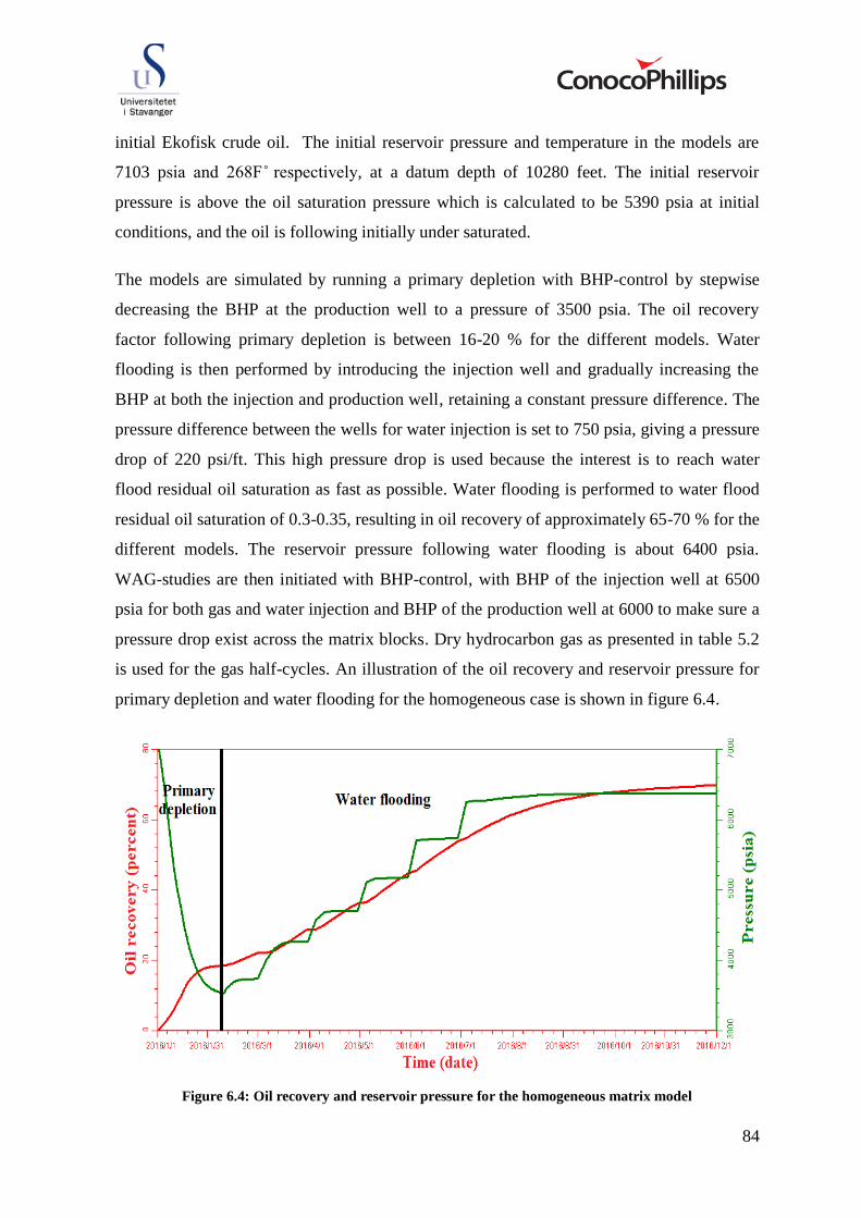
84
initial Ekofisk crude oil. The initial reservoir pressure and temperature in the models are
7103 psia and F respectively, at a datum depth of 10280 feet. The initial reservoir
pressure is above the oil saturation pressure which is calculated to be 5390 psia at initial
conditions, and the oil is following initially under saturated.
The models are simulated by running a primary depletion with BHP-control by stepwise
decreasing the BHP at the production well to a pressure of 3500 psia. The oil recovery
factor following primary depletion is between 16-20 % for the different models. Water
flooding is then performed by introducing the injection well and gradually increasing the
BHP at both the injection and production well, retaining a constant pressure difference. The
pressure difference between the wells for water injection is set to 750 psia, giving a pressure
drop of 220 psi/ft. This high pressure drop is used because the interest is to reach water
flood residual oil saturation as fast as possible. Water flooding is performed to water flood
residual oil saturation of 0.3-0.35, resulting in oil recovery of approximately 65-70 % for the
different models. The reservoir pressure following water flooding is about 6400 psia.
WAG-studies are then initiated with BHP-control, with BHP of the injection well at 6500
psia for both gas and water injection and BHP of the production well at 6000 to make sure a
pressure drop exist across the matrix blocks. Dry hydrocarbon gas as presented in table 5.2
is used for the gas half-cycles. An illustration of the oil recovery and reservoir pressure for
primary depletion and water flooding for the homogeneous case is shown in figure 6.4.
Figure 6.4: Oil recovery and reservoir pressure for the homogeneous matrix model
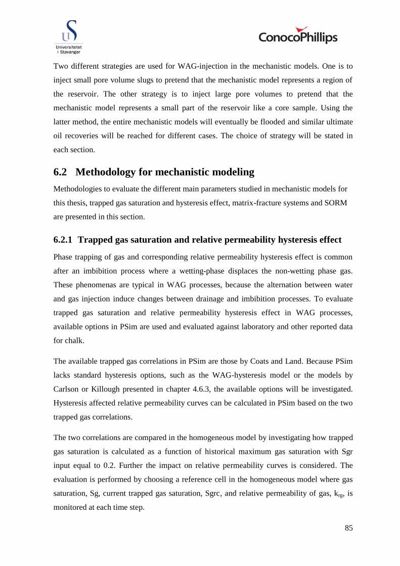
85
Two different strategies are used for WAG-injection in the mechanistic models. One is to
inject small pore volume slugs to pretend that the mechanistic model represents a region of
the reservoir. The other strategy is to inject large pore volumes to pretend that the
mechanistic model represents a small part of the reservoir like a core sample. Using the
latter method, the entire mechanistic models will eventually be flooded and similar ultimate
oil recoveries will be reached for different cases. The choice of strategy will be stated in
each section.
6.2 Methodology for mechanistic modeling
Methodologies to evaluate the different main parameters studied in mechanistic models for
this thesis, trapped gas saturation and hysteresis effect, matrix-fracture systems and SORM
are presented in this section.
6.2.1 Trapped gas saturation and relative permeability hysteresis effect
Phase trapping of gas and corresponding relative permeability hysteresis effect is common
after an imbibition process where a wetting-phase displaces the non-wetting phase gas.
These phenomenas are typical in WAG processes, because the alternation between water
and gas injection induce changes between drainage and imbibition processes. To evaluate
trapped gas saturation and relative permeability hysteresis effect in WAG processes,
available options in PSim are used and evaluated against laboratory and other reported data
for chalk.
The available trapped gas correlations in PSim are those by Coats and Land. Because PSim
lacks standard hysteresis options, such as the WAG-hysteresis model or the models by
Carlson or Killough presented in chapter 4.6.3, the available options will be investigated.
Hysteresis affected relative permeability curves can be calculated in PSim based on the two
trapped gas correlations.
The two correlations are compared in the homogeneous model by investigating how trapped
gas saturation is calculated as a function of historical maximum gas saturation with Sgr
input equal to 0.2. Further the impact on relative permeability curves is considered. The
evaluation is performed by choosing a reference cell in the homogeneous model where gas
saturation, Sg, current trapped gas saturation, Sgrc, and relative permeability of gas, krg, is
monitored at each time step.

86
To evaluate the best matching trapped gas correlation and Sgr input value for the Ekofisk
chalk, simulations results are compared with reported data on chalks and laboratory results
by ConocoPhillips on trapped gas. Sgr input values of 0.2, 0.3 and 0.35 for Lands
correlation and Sgr input values of 0.2 and 0.5 for Coats correlation are studied. The
evaluation is done by comparing how trapped gas saturation is calculated as a function of
historical maximum gas saturation and comparing this with reported and laboratory data.
The same reference cell as used earlier is used to obtain data for the evaluation.
Finally an evaluation of the impact trapped gas saturation has on a WAG-process is done by
comparing the best matching Sgr-input value with a run where trapped gas is negligible,
Sgr=Sgc=0.05. Trapped gas of 0.05 equals a run where trapped gas is neglected, since the
critical gas saturation is 0.05. In each sensitivity run all parameters other than Sgr are
unchanged and kept equal to the standard, presented in section 6.1. The homogeneous
matrix model is assumed to be a larger part of a reservoir and small slugs are therefore
injected in this evaluation.
6.2.2 Matrix-fracture systems
In the Ekofisk chalk reservoirs it is the naturally fractures that makes the reservoirs
producible. The Ekofisk field has different types of fractures making up different kind of
Ffracture-networks within the matrix. The different matrix-fracture systems lead to different
flow performance in the reservoir resulting in different oil production from a WAG-process
in different regions. Five matrix-fracture models are designed in this thesis to investigate the
impact of different matrix-fracture systems within a reservoir and their impact on WAG-
displacement. All matrix grid blocks and all fracture grid blocks within the different models
have similar properties, as presented in section 6.1. The five different models design for the
matrix-fracture evaluation are:
1) Homogeneous matrix model with no fractures.

87
2) 3-layer fracture model with three horizontal layered fractures introduced within the
matrix model, illustrated in figure 6.5.
Figure 6.5: 3-layer fracture model in the xz-plane
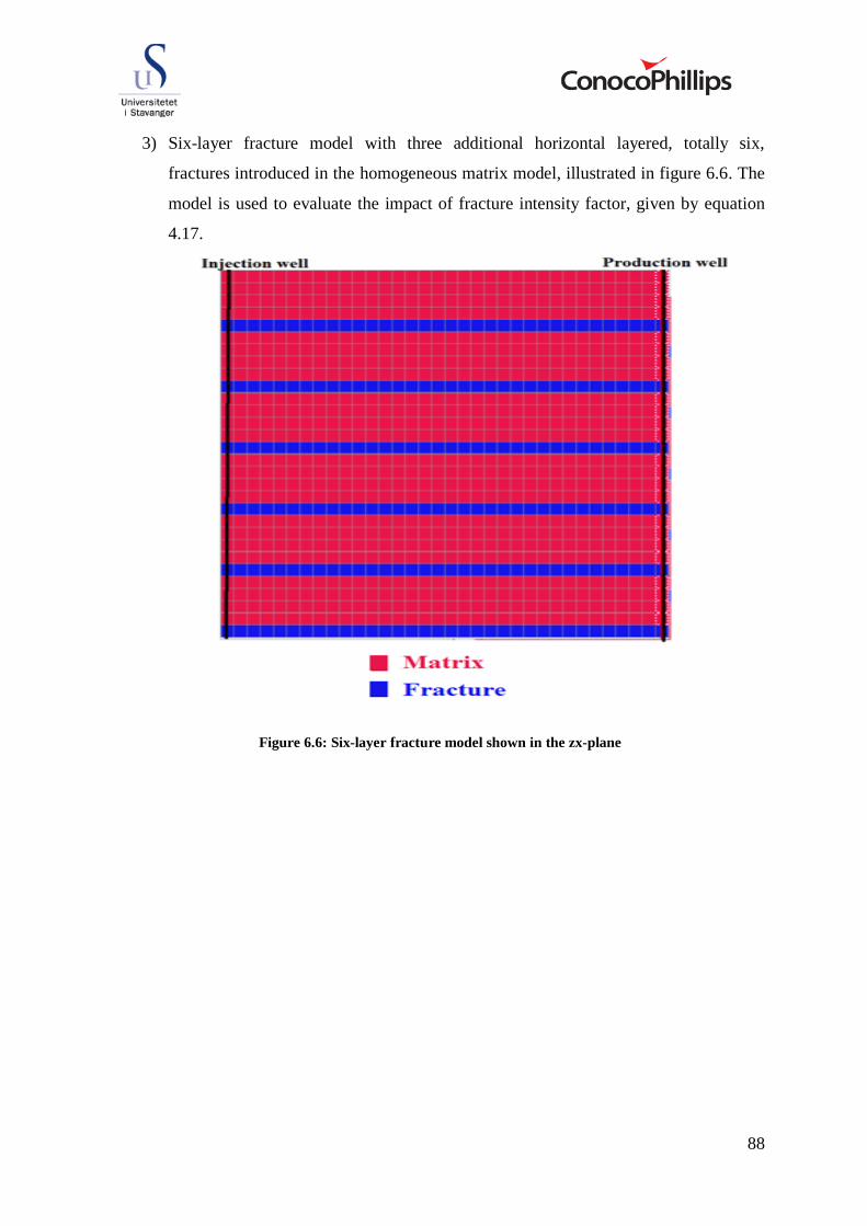
88
3) Six-layer fracture model with three additional horizontal layered, totally six,
fractures introduced in the homogeneous matrix model, illustrated in figure 6.6. The
model is used to evaluate the impact of fracture intensity factor, given by equation
4.17.
Figure 6.6: Six-layer fracture model shown in the zx-plane

89
4) Discontinuous fracture model with three discontinuous fractures introduced within
the homogeneous matrix model, illustrated in figure 6.7.
Figure 6.7: Discontinuous fracture model in the xz-plane
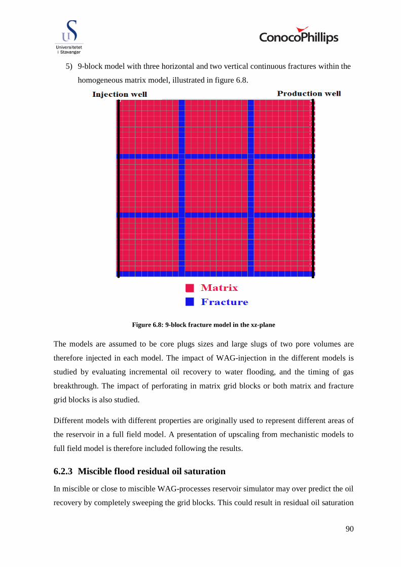
90
5) 9-block model with three horizontal and two vertical continuous fractures within the
homogeneous matrix model, illustrated in figure 6.8.
Figure 6.8: 9-block fracture model in the xz-plane
The models are assumed to be core plugs sizes and large slugs of two pore volumes are
therefore injected in each model. The impact of WAG-injection in the different models is
studied by evaluating incremental oil recovery to water flooding, and the timing of gas
breakthrough. The impact of perforating in matrix grid blocks or both matrix and fracture
grid blocks is also studied.
Different models with different properties are originally used to represent different areas of
the reservoir in a full field model. A presentation of upscaling from mechanistic models to
full field model is therefore included following the results.
6.2.3 Miscible flood residual oil saturation
In miscible or close to miscible WAG-processes reservoir simulator may over predict the oil
recovery by completely sweeping the grid blocks. This could result in residual oil saturation

91
(SORM) approaching zero. As presented in chapter 4.7, this is unlikely to occur in field
cases for several reasons. To avoid over estimation of oil recovery in full field simulations
several methods have been proposed. Two methods, SORM options, are available in PSim
to account for the problem, discussed in detail in chapter 4.7.
To evaluate how the different SORM options operate, simulations with input SORM of 0.2
are performed in the homogeneous matrix model for both options. Since the main interest is
to capture how the options operate at low oil saturations, the homogeneous matrix model is
used and assumed to be core plug size and therefore entirely flodded with two pore volumes
slugs.
To account for SORM in full-field reservoir simulations of WAG-processes the incremental
recovery from the different matrix-fracture mechanistic models is used as a basis for SORM
in the upscaled grid blocks in the sector model.
6.3 Results and discussion of mechanistic simulations
The results from mechanistic simulations are presented in this section, divided into trapped
gas saturation and relative permeability hysteresis effect, matrix-fracture systems and
miscible flood residual oil saturation.
6.3.1 Trapped gas saturation and relative permeability hysteresis effect
Simulations were run in the homogeneous matrix model with input Sgr equal to 0.2 to
evaluate how trapped gas saturation is calculated for the different trapped gas correlations in
PSim. The reference cell (18,1,18) was chosen to monitor how trapped gas saturation is
calculated as a function of maximum historical gas saturation, plotted in figure 6.9,
assuming that a complete imbibition process is initiated at the maximum historical gas
saturation.

92
Figure 6.9: Land and Coats trapped gas saturation as function of maximum historical gas saturation for
reference grid block (18,1,18)
Land’s non-linear correlation relates the amount of gas being trapped to the maximum
historical gas saturation by applying equation 4.8, where CLand is calculated by equation 4.9
to be 4, based on the input Sgr value of 0.2. In example the black box on the Land non-
linear curve has the gas saturation of 0.1669. Assuming this is the maximum historical gas
saturation at the start of a complete imbibition process, the trapped gas saturation is
calculated by applying equation 4.8:
Coats correlation relates the amount gas being trapped to the maximum historical gas
saturations by using the linear correlation given in equation 4.14. The trapping constant C,
given by equation 4.15, is 0.1648 corresponding to the slope of Coats curve in figure 6.9. In
example the blue box on Coats curve has the gas saturation of 0.3458. The trapped gas
saturation, assuming this gas saturation is the maximum historical gas saturation at the start
of a complete imbibition process, is calculated by applying equation 4.14:
0
0,02
0,04
0,06
0,08
0,1
0,12
0,14
0,16
0,18
0,2
0 0,1 0,2 0,3 0,4 0,5 0,6
Tra
pp
ed
ga
s s
atu
rati
on
Maximum historical gas saturation
Trapped gas saturation as function of max gas saturation for different correlation using input Sgr=0.2
Land non-linear
Coats

93
Gas trapping can in both cases only occur if the gas saturation increases above the critical
gas saturation at 0.05, because an imbibition process subsequent to a drainage process can
only occur when gas is flowing, accordingly above the critical gas saturation.
To find gas relative permeability curves corresponding to the two correlations, the reference
cell (18,1,18) was used to monitor gas saturation and gas relative permeability as a function
of time. Gas relative permeability as a function of gas saturation in the first WAG gas cycle,
drainage process, and first WAG water cycle, imbibition process is plotted in figure 6.10,
for the two different correlations.
Figure 6.10: Gas relative permeability curves for Coats and Lands correlations with input maximum
trapped gas saturation of 0.2 based on data from the reference grid block (18,1,18)
To calculate the hysteresis effected imbibition curve, maximum gas saturation in the start of
the imbibition process is used to calculate the amount of trapped gas of a complete
imbibition. At any point along the imbibition process relative permeability is calculated
based on the mobile part of the total gas saturation, given by equation 4.12. The mobile gas
saturation is then used to calculate hysteresis effected relative permeability data in the
imbibition process by applying equation 4.13.
0
0,05
0,1
0,15
0,2
0,25
0,3
0 0,1 0,2 0,3 0,4 0,5 0,6
Krg
Sg
Imbibition curves for different trapped gas correlations
Drainage
Coats imbibition
Land non-linear imbibition

94
The drainage curve for the next WAG gas cycle will follow the imbibition curve, possibly
up to the maximum gas saturation achieved during previous drainage process, and then
along the input relative permeability curve if gas saturation is further increased.
To evaluate which trapped gas correlation and Sgr input value that matches best with chalk,
simulation results for different Sgr input values for both correlations were compared with
reported (Keelan, et al., 1975) and laboratory data (Maloney, 2003) on trapped gas (shown
in figure 6.11)
Figure 6.11: Trapped gas correlations and different Sgr-input values compared to reported and
laboratory data on trapped gas
0
0,05
0,1
0,15
0,2
0,25
0,3
0,35
0 0,2 0,4 0,6 0,8 1
Tra
pp
ed
gas s
atu
rati
on
Historical maximum gas saturation
Keelan and Pugh Chalk trapped gas results Laboratory trapped gas data from chalk core samples Land non-linear correlation with input Sgr=0.35 Land non-linear correlation with input Sgr=0.2 Land non-linear correlation with input Sgr=0.3 Coats correlation inpt Sgr=0.5
Coats correlation with input Sgr=0.2
95
Land’s correlation with input Sgr of 0.35, the yellow curve in figure 6.11, matches the
laboratory data and Keelan and Pughs trapped gas data on chalk the best. Based on this
result the homogeneous model with Land’s correlation and Sgr-value of 0.35 will be
compared to a run with negligible trapped gas. Sgr-value of 0.35 will also be used as basis
for sector modeling.
Two sensitivity runs were carried out with Sgr equal to 0.05 and 0.35, and all other
parameters kept unchanged from the properties presented in section 6.1. Five WAG-cycles
were injected with half-cycle slug sizes of 0.1 pore volumes. In figure 6.12 the oil recovery
is plotted as function of time to for the two cases. To get a better understanding what
happens in the simulations, gas saturation, oil saturation, oil saturation pressure and
reservoir pressure where plotted for the reference grid block (18,1,18) as a function of time
for both cases (shown in appendix C).
Figure 6.12: Impact of trapped gas on oil recovery for WAG-displacement
No effect of trapped gas is observed during the primary deletion period because this is a
drainage process where the gas saturation increases. As water injection is initiated, the gas
saturation decreases, hence starts an imbibition process where gas trapping can occur. From
the reference cell, the gas saturation obtained after primary depletion is 0.285. Based on the
maximum historical gas saturation, Land’s correlation calculates the trapped gas, for Sgr
input of 0.35, to be 0.188. The gas relative permeability is lower during imbibition than
during drainage because gas is gradually being trapped. During water injection gas

96
eventually becomes immobile at the gas saturation of 0.188. As the pressure increases due
to water flooding, the pressure will eventually increases above the oil saturation pressure
and gas will go into solution with oil. When gas goes into solution, the oil saturation
pressure will increase. Eventually as pressure is further increased all gas will be in solution
with the oil and no trapped gas is left in the reservoir. For the case with trapped gas
included, more gas will go in solution because more gas is present. Following water
flooding the oil recovery from both cases are similar, as illustrated in figure 6.12. The case
with negligible trapped gas saturation though has a higher gas recovery, and following a
higher oil equivalent recovery than the case where gas.
When gas injection in the WAG-process is initiated the reservoir pressure will be above the
oil saturation pressure, and gas will go in solution until the oil saturation pressure exceeds
the reservoir pressure. The amount gas going into solution is equal for both runs because no
gas is present in the reservoir following water flooding. When gas is injected at reservoir
pressure lower than the oil saturation pressure, free gas will start develop in the grid blocks
and increase till the end of the drainage process. Gas trapping will occur during the
subsequent water injection, and hence imbibition process. The oil recovery following WAG-
injection is 2 % higher when trapped gas is neglected compared to the case with input Sgr of
0.35. Similarly the gas recovery following WAG-injection is 35 % higher when trapped gas
is neglected. This illustrates that neglecting trapped gas will give an optimistic prediction of
both oil and gas recovery.
6.3.2 Matrix-fracture systems
The matrix-fracture models presented in section 6.2.2 were all run using the simulation
procedure presented in section 6.1. Two different strategies were investigated, perforating
only in matrix grid blocks and perforating in both matrix and fracture grid blocks. Table 6.4
and figure 6.13 show the oil recovery after water flood and after WAG injection for the different
models with perforation in matrix grid blocks only.

97
Table 6.4: Oil recoveries for the matrix-fracture models perforated in matrix only
Model Type
Water flood recovery
WAG recovery
Incremental recovery
Homogeneous matrix model 69.4 % 93.7 % 24.3 %
3-layer fracture model 66.5 % 80.9 % 14.4 %
6-layer fracture model 65.0 % 76.3 % 11.3 %
Discontinuous fracture model 69.4 % 91.5 % 22.1 % 9-block fracture
model 65.2 % 77.8 % 12.6 %
Figure 6.13: Oil recovery for the matrix-fracture models perforated in matrix only
The incremental oil recovery above water flood clearly shows the impact of fractures,
ranging from 11 % incremental oil recovery for high fracture intensity factor to 22 % with
low fracture intensity factor.
The reason for difference in oil recovery between the matrix system and the matrix-fracture
systems is that injected fluid will tend to flow into the high permeable fractures and

98
displacement of oil in the matrix becomes less efficient. As the number of fractures is
increased, the volume injected fluid going into the fractures increases and hence decreased
displacement efficiency in the matrix blocks is observed. Gas saturation in the 3-layer and
the 6-layer fracture model early in the WAG-process are illustrated in figure 6.14 and 6.15.
Figure 6.14: Gas saturation in the 3-layer fracture model
Figure 6.15: Gas saturation in the 6-layer fracture model
For the discontinuous fracture model, gas is forced out of the fractures and into the matrix.
This will result in better matrix sweep efficiency compared to the continuous fracture
models and hence high recovery, slightly less than what is observed for the homogeneous
matrix model.

99
For the 9-block fracture model, the sweep of injected fluid in the grid blocks close to the
injection well is good, however as injected fluid reach the fracture, it follows the fracture all
the way to production well which result in poor sweep of the middle matrix blocks,
illustrated in figure 6.16. The reason for high gas saturations in the matrix grid blocks close
to the production well is that the production well is perforated in the matrix only, and gas
has to enter the matrix block by any of the mechanisms described in chapter 4.9.2.1 to be
produced.
Figure 6.16: Gas saturation in the 9-block fracture model
Table 6.5 and figure 6.17 show the oil recovery after water flood and after WAG injection for the
different models with perforation in both matrix and fracture grid blocks only.
Table 6.5: Oil recoveries for the matrix-fracture models perforated in both matrix and fractures
Model Type
Water flood recovery
WAG recovery
Incremental recovery
Homogeneous matrix model 69.4 % 93.7 % 24.3 %
3-layer fracture model 66.9 % 78.7 % 11.8 %
6-layer fracture model 66.0 % 74.3 % 8.3 %
Discontinuous fracture model 69.0 % 89.5 % 20.5 % 9-block fracture
model 64.3 % 72.3 % 8.0 %

100
Figure 6.17: Oil recovery for the matrix-fracture models perforated in matrix and fracture grid blocks
When perforating in both matrix and fracture grid blocks lower oil recoveries are observed,
compared to perforation only in matrix grid blocks. Incremental oil recoveries to water
flood ranges from 8 % in high fractured areas to 20 % in areas with low fracture intensity
factor. The difference in incremental oil recoveries between perforations in matrix only and
in both matrix and fractures are between 2 to 5 %. The reason for this is that gas is forced
into the matrix blocks before it can reach the fractures when perforating in the matrix only,
hence giving a better sweep efficiency and better oil recovery.
Because the exact locations of different fractures in the reservoir are not known, the wells
are commonly perforated in both matrix and fractures. Based on well test data, indicating
high effective permeability, one has an idea of areas with high degree of fractures and
perforating wells in these areas can therefore be avoided. Production wells though are
always perforated along the entire reservoir region where it is believed to be oil.
Upscaling
The grid blocks used in the mechanistic models are far too fine to be used as grids in full
field reservoir models. All grids within a high resolution mechanistic model may be
represented by only one or a few grid blocks in a full field model. To close the gap
upscaling from mechanistic models are used to make single grid blocks represent the same

101
behavior as entire mechanistic models. An example is how different matrix-fracture system
should be represented by single coarse grid blocks in a low resolution full field model. This
means that both matrix and fractures needs to be described within the same grid block and
alteration of parameters between the scales is necessary. Input parameters to mechanistic
models may be obtained by fluid samples, core samples, laboratory work and well testing.
The ultimate goal of upscaling is to construct low resolution models which mimic the
recovery characteristics of the higher resolution models. To do this reservoir parameters and
reservoir performance in high resolution models are matched in low resolution models. The
upscaling technique may involve averaging of reservoir parameters and alteration of relative
permeability curves in the low resolution model to match flow behavior and important
factors affecting the recovery efficiency in the higher resolution models.
Upscaling techniques have been applied to give properties to the grid block in the Ekofisk
full field simulation model. Based on the grid properties, if-functions have been used to
assign each grid block to a set of relative permeability curves representing different kind of
systems.
In this study a sector model, region of the full field model, is used which already have been
upscaled. However, trapped gas saturation and SORM will be altered according to the
results obtained in this chapter of the thesis.
6.3.3 Miscible flood residual oil saturation
SORM is introduced to avoid over prediction of oil recovery when the matrix-fracture
models are upscaled into the sector model. Since the mechanistic matrix-fracture models
gave significant differences in oil recoveries, different SORM-values need to be assigned to
different grid blocks in the sector model representing different matrix-fracture models.
The matrix-fracture models have different effective permeability which is used as a basis to
upscale SORM to grid blocks in the sector model. This is done by using setting SORM
values in grid blocks based on the horizontal permeability. Within different ranges of
horizontal permeability different SORM-values are assigned.
The homogeneous matrix model is used to represent areas without fractures. As the matrix
permeability is believed to range between 1 to 4 mD, all grid blocks in the sector model
with horizontal permeability less than 4 mD are assigned SORM-values of 0.06 which
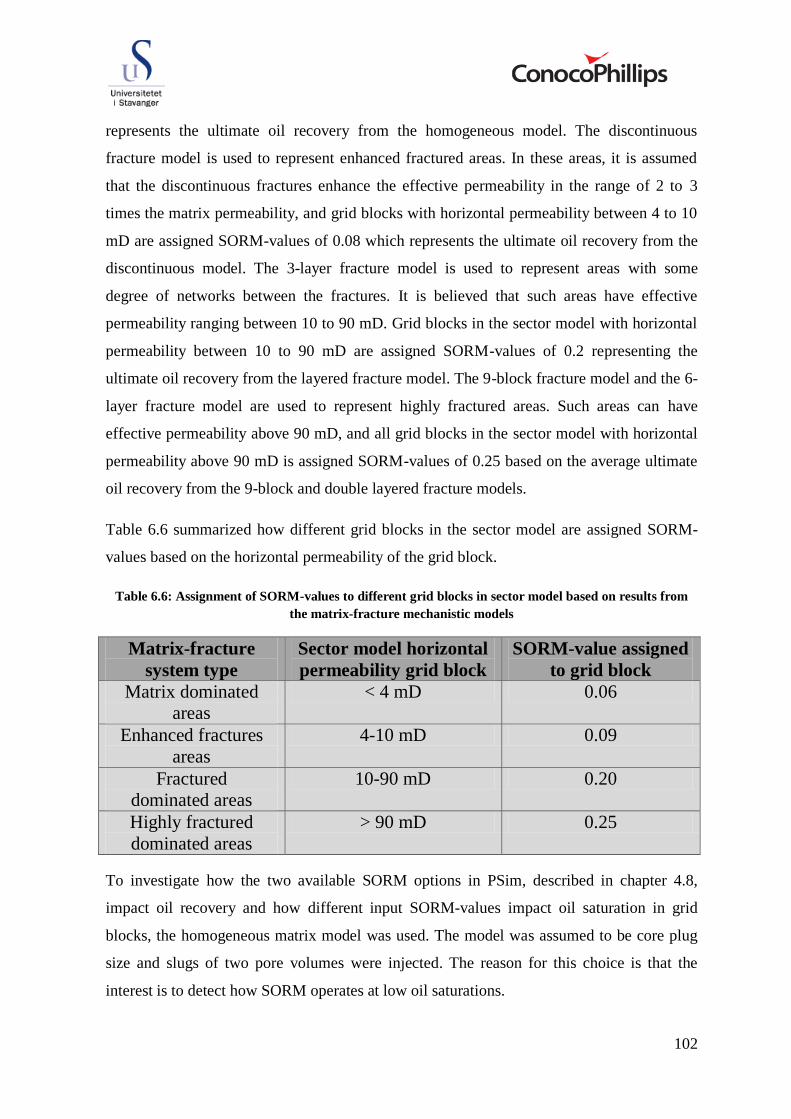
102
represents the ultimate oil recovery from the homogeneous model. The discontinuous
fracture model is used to represent enhanced fractured areas. In these areas, it is assumed
that the discontinuous fractures enhance the effective permeability in the range of 2 to 3
times the matrix permeability, and grid blocks with horizontal permeability between 4 to 10
mD are assigned SORM-values of 0.08 which represents the ultimate oil recovery from the
discontinuous model. The 3-layer fracture model is used to represent areas with some
degree of networks between the fractures. It is believed that such areas have effective
permeability ranging between 10 to 90 mD. Grid blocks in the sector model with horizontal
permeability between 10 to 90 mD are assigned SORM-values of 0.2 representing the
ultimate oil recovery from the layered fracture model. The 9-block fracture model and the 6-
layer fracture model are used to represent highly fractured areas. Such areas can have
effective permeability above 90 mD, and all grid blocks in the sector model with horizontal
permeability above 90 mD is assigned SORM-values of 0.25 based on the average ultimate
oil recovery from the 9-block and double layered fracture models.
Table 6.6 summarized how different grid blocks in the sector model are assigned SORM-
values based on the horizontal permeability of the grid block.
Table 6.6: Assignment of SORM-values to different grid blocks in sector model based on results from
the matrix-fracture mechanistic models
Matrix-fracture
system type
Sector model horizontal
permeability grid block
SORM-value assigned
to grid block
Matrix dominated
areas
< 4 mD 0.06
Enhanced fractures
areas
4-10 mD 0.09
Fractured
dominated areas
10-90 mD 0.20
Highly fractured
dominated areas
> 90 mD 0.25
To investigate how the two available SORM options in PSim, described in chapter 4.8,
impact oil recovery and how different input SORM-values impact oil saturation in grid
blocks, the homogeneous matrix model was used. The model was assumed to be core plug
size and slugs of two pore volumes were injected. The reason for this choice is that the
interest is to detect how SORM operates at low oil saturations.

103
The effect the two different options have on oil recovery using input SORM value of 0.2 is
compared with a run where SORM options are excluded, shown in figure 6.18.
Figure 6.18: Oil recovery for the different SORM options in PSim, and a run without SORM
To get a better understanding how the different options cope with oil saturation, oil
saturation as a function of time is plotted for the reference cell (18,1,1), as illustrated in
figure 6.19.
Figure 6.19: Oil saturation as a function of time in the reference grid block (18,1,18) for the two
available SORM options in PSim, and the run without SORM
0
0,1
0,2
0,3
0,4
0,5
0,6
0,7
0,8
0,9
1
01.01.2016 01.04.2016 01.07.2016 30.09.2016 30.12.2016 31.03.2017 30.06.2017
Oil s
atu
rati
on
Time (date)
SORM Default
SORM Sotrig
No SORM

104
It is observed from, from figure 6.18 and 6.19, that the SORM Sotrig option and the case
without SORM are equal for primary depletion and water flooding. The default SORM
option though differs from these two cases for the same period. The reason for this is that
for the default SORM option, 20 % of the total oil saturation is considered to be isolated in a
different medium and this oil will not contribute to phase behavior calculations. This means
that mass exchange through vaporization and condensation between the isolated oil and the
flowing hydrocarbons is not described as for the other two cases.
The SORM Sotrig option will not affect the performance of primary depletion and water
flooding, because SORM first takes effect for a grid block when the oil saturation becomes
less than or equals to the input SORM value. This means that all oil contribute to phase
behavior calculation until the input SORM value is reached.
Since choice of SORM option should not affect primary depletion and water flooding, rather
set a limit for oil depletion from grid blocks, the SORM Sotrig option is chosen for further
studies.
The effect on oil recovery and on grid block oil saturation for input SORM values of 0.03
and 0.2 using the SORM Sotrig option is shown in figure 6.20 and figure 6.21 respectively.
Figure 6.20: Effect of different input SORM values to oil recovery for SORM Sotrig option

105
Figure 6.21: Oil saturation as a function of time for different SORM input values for the reference grid
block
It is observed that the grid block oil saturations are equal until the oil saturation becomes
0.2. At this saturation SORM will be trigged for the case with user-defined SORM value of
0.2, meaning that further oil depletion from the grid block is not possible. For the case with
input SORM value of 0.03, further depletion can occur until the oil saturation reaches 0.03.
0
0,1
0,2
0,3
0,4
0,5
0,6
0,7
0,8
0,9
1
01.01.2016 01.04.2016 01.07.2016 30.09.2016 30.12.2016 31.03.2017 30.06.2017
Oil s
atu
rati
on
Time (date)
SORM=0.2
SORM=0.03

106

107
7 Sector modeling
A sector model is a section of the Ekofisk full field simulation model. The sector model
used in this thesis is shown within the red box on figure 7.1. The sector model uses the same
grid blocks, wells, faults and properties as that section of the full field simulation model.
The sector model is introduced in this thesis to study how different WAG ratios and half-
cycle slug sizes effects production performance and oil recovery on field-scale.
Figure 7.1: Ekofisk full field model, illustrating the location of the sector model within the red square

108
7.1 Description and methodology for sector model
The sector model comprises a history matched part from 1971 to 2011 and a predictive part
from 2011 till end of license in 2028. The history matched part is based on historical data
from production and injection wells, on reservoir pressure and fluid flow. Production and
injection data are such as rates, pressures, water-cuts, GOR. Knowledge about fluid flow is
through tracers, saturation of cores, breakthrough times and 4D seismic. The predictive part
gives the opportunity to visualize and compare the continued water flood scenario to WAG
scenarios.
Model description
The sector model is a single porosity/single permeability system where the effective
porosity and effective permeability are entered for each grid cell. The effective porosity and
permeability is calculated from estimated matrix and fracture properties. The model has 22
vertical layers. The division of the Ekofisk formation and Tor formation into the 22 vertical
layers is shown in figure 7.2. The sector model is run in compositional mode with the 7-
component Peng-Robinson EOS presented in table 6.3 of chapter 6.1.
The sector model consists of 17600 grid blocks, 5∙ ∙ grids in the x-, y-, z-directions
respectively. Only 16244 of the grid blocks are active. Each grid block has size of
approximately 225 feet in the x-direction, 240 feet in the y-direction and thickness of
average 40 feet. All grid blocks within the sector model have been assigned a set of initial
properties such as initial fluid saturations, effective permeability and porosity, and a set of
relative permeability curves, stress tables and compaction tables based on upscaling
techniques. The stress and compaction tables are used to alter permeability and porosity
respectively as a function of pressure to account for the subsidence observed at the Ekofisk
field. Three-phase relative permeability data are calculated by Stone’s method. Capillary
pressure curves are not included in the sector model
The input porosities range from 0.15 to 0.40 with an average of 0.26. The horizontal
permeability ranges from zero, in the impermeable tight zone, up to 720 mD, in the most
fractured areas. The average horizontal permeability is 6 mD. Input maximum trapped gas
saturation is set to 0.35 with trapped gas calculated by Lands correlation, and SORM values
are assigned based on horizontal permeability data as discussed in chapter 6.3.3 using the
SORM Sotrig option.
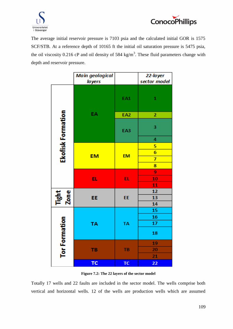
109
The average initial reservoir pressure is 7103 psia and the calculated initial GOR is 1575
SCF/STB. At a reference depth of 10165 ft the initial oil saturation pressure is 5475 psia,
the oil viscosity 0.216 cP and oil density of 584 kg/m3. These fluid parameters change with
depth and reservoir pressure.
Figure 7.2: The 22 layers of the sector model
Totally 17 wells and 22 faults are included in the sector model. The wells comprise both
vertical and horizontal wells. 12 of the wells are production wells which are assumed

110
operated since 1972 and five are water injection wells assumed operating since 1984. The
distribution of the wells and faults in the sector model is shown in figure 7.3, as black dots
and black lines between grid blocks. The initial reservoir pressure of the top layer is also
illustrated in the figure 7.3.
Figure 7.3: Initial reservoir pressures and distribution of wells and faults in the sector models upper
layer 1.

111
Base case simulation
A base case simulation of continued water injection for all the injection wells till the end of
license in 2028 is used to compare with different WAG scenarios. All wells are operated
with BHP-control and maximum rate limits. The limiting BHP is set to 2 000 psia for
production wells and to 7 000 psia for injection wells. The maximum production rate is set
to 2 000 STB/D and maximum injection rate to 10 000 BWPD.
The oil recovery and average reservoir pressure as a function of time is shown for the base
case simulation in figure 7.4.
Figure 7.4: Oil recovery and average pressure for the base case simulation in the sector model
The oil recovery after primary depletion is around 12 % and the oil recovery following
water flooding till the end of license in 2028 is 23.9 %. These recoveries are a lot lower than
what is observed in the field and within the Ekofisk full field simulation model. The reason
for the low recoveries in the sector model is that only wells within the region of the sector
model are included. In reality, surrounding production and injection well will result in a
more extensive water flooding and better depletion than what is modeled within the sector
model. However, the sector model can be used to investigate the incremental oil recovery
for WAG scenarios within the given model and results can be compared to the water
scenario base case. Figure 7.4 further illustrates that if WAG-injection is initiated after
water flooding till 2018, the average reservoir pressure would be above 7100 psia. This

112
reservoir pressure is above the minimum miscibility pressure for all temperatures, presented
in chapter 5.3.1, and miscible displacement would likely be achieved.
WAG-injection
For WAG scenarios the former water injection well, well B16W, is changed to a WAG-
injection well, B16WAG, for the predictive part starting from 2011. This well is shown in
the circle in figure 7.3. The injection well, B16WAG, is a vertical well which is
representative for both formations as it is perforated in the Ekofisk formation in layer 1-9
and 11, and in the Tor formation in layer 16-19. Layer 10 and 15 are not represented in the
well because of a pinch-out, while layer 12-14 are in the tight zone. All wells are still
operated under BHP-control and maximum rate limits, similar to what was presented for the
base case. The only difference is that the WAG injection well is switched to a BHP limit of
8 000 psia, which is obtainable, to ensure high injection rates.
Methodology
Methodology WAG-ratios
For the Ekofisk reservoir it is believed that low vertical permeability will result in limited
flow in the vertical direction and also that most injected gas flows along fractured areas,
which together results in poor macroscopic sweep efficiency. However, optimizing the
WAG-ratio, ratio of volume of water injected to gas injected, can result in increased oil
recovery. The water slugs stabilizes the gas front by a more favorable displacement mobility
ratio, which results in better sweep efficiency, as reduced viscous fingering and postponed
gas breakthrough can be obtained.
To study the effect of WAG ratio on recovery for this sector model, four different cases with
WAG ratio 4:1, 2:1, 1:1 and 1:2 are simulated and compared with the base case. The gas
half-cycle slug sizes are set to 10 % of the pore volume of the grid size which the water
injection well, B16W, had swept by 2011. This pore volume equals approximately 100
million barrels and each gas-half cycle equals 10 million barrels or roughly 56 million cubic
feet. In each case three WAG-cycles are used, meaning a total of 0.3 pore volumes of gas
injected for each case.

113
Methodology WAG slug sizes
Optimization of the size of injected slugs of water and gas can result in increased oil
recovery. Smaller WAG slug sizes will result in an increase zone of three flowing phases,
which can result in better displacement efficiency.
To study the effect different slug sizes have on oil recovery, four WAG cases with half-
cycle slug sizes of 0.05, 0.1, 0.2 and 0.4 pore volumes are simulated. WAG ratio of 1:1 is
used for the different cases. For evaluation the total amount of gas injected should be equal
and is set to 0.4 pore volumes, which will control number of WAG-cycles for each case.
7.2 Results and discussion of sector simulations
7.2.1 WAG-ratio
Different WAG-ratios are evaluated by the amount of barrels of oil equivalent (BOE) going
to sale, compared to the water flood base case. The BOE to sale is obtained by using a
ConocoPhillips tool, based on the simulation output. BOE to sale is calculated based on oil
production rates, gas production rates, fuel, gas injection and sales factors and is shown in
appendix D for the different WAG ratios. The cumulative incremental BOE to the base case
is plotted in figure 7.5 and summarized in table 7.1
Figure 7.5: Cumulative incremental barrels of oil equivalent to water flood base case for different WAG
ratios
-2
0
2
4
6
8
10
2012 2014 2016 2018 2020 2022 2024 2026 2028
Cu
mu
lati
ve in
cre
men
tal
BO
E (
millio
ns)
Time (years)
WAG-ratio 1:2
WAG-ratio 1:1
WAG ratio 2:1
WAG ratio 4:1

114
Table 7.1: Barrels of oil equivalent and incremental barrels of oil equivalent to base case for different
WAG ratios for the predictive part from 2011 to 2028
Scenario BOE to sale at the end of
the predictive period
( for year 2011-2028)
Incremental BOE to
sale to the base case
Water flood base case 17.5 million BOE -
WAG ratio 1:1 24.4 million BOE 6.9 million BOE
WAG ratio 2:1 21.8 million BOE 4.3 million BOE
WAG ratio 4:1 20.4 million BOE 2.9 million BOE
WAG ratio 1:2 25.9 million BOE 8.4 million BOE
It is observed that the best WAG scenario is with WAG ratio of 1:2 which gives additional
8.4 million BOE to sale compared to the water flood base case. Figure 7.5 and table 7.1
indicates that decreased WAG-ratios results in increased oil equivalent recovery. For all the
WAG scenarios incremental oil equivalent recovery to the water flood base case is
observed.
A plot of gas saturation and permeability for layer 8 is given in figure 7.6 to illustrate the
flow pattern of injected gas.
Figure 7.6: Gas saturation and permeability in layer 8 of the sector model during WAG injection
It is seen from figure 7.6 that most of the injected gas will flow in the high permeable grid
blocks.
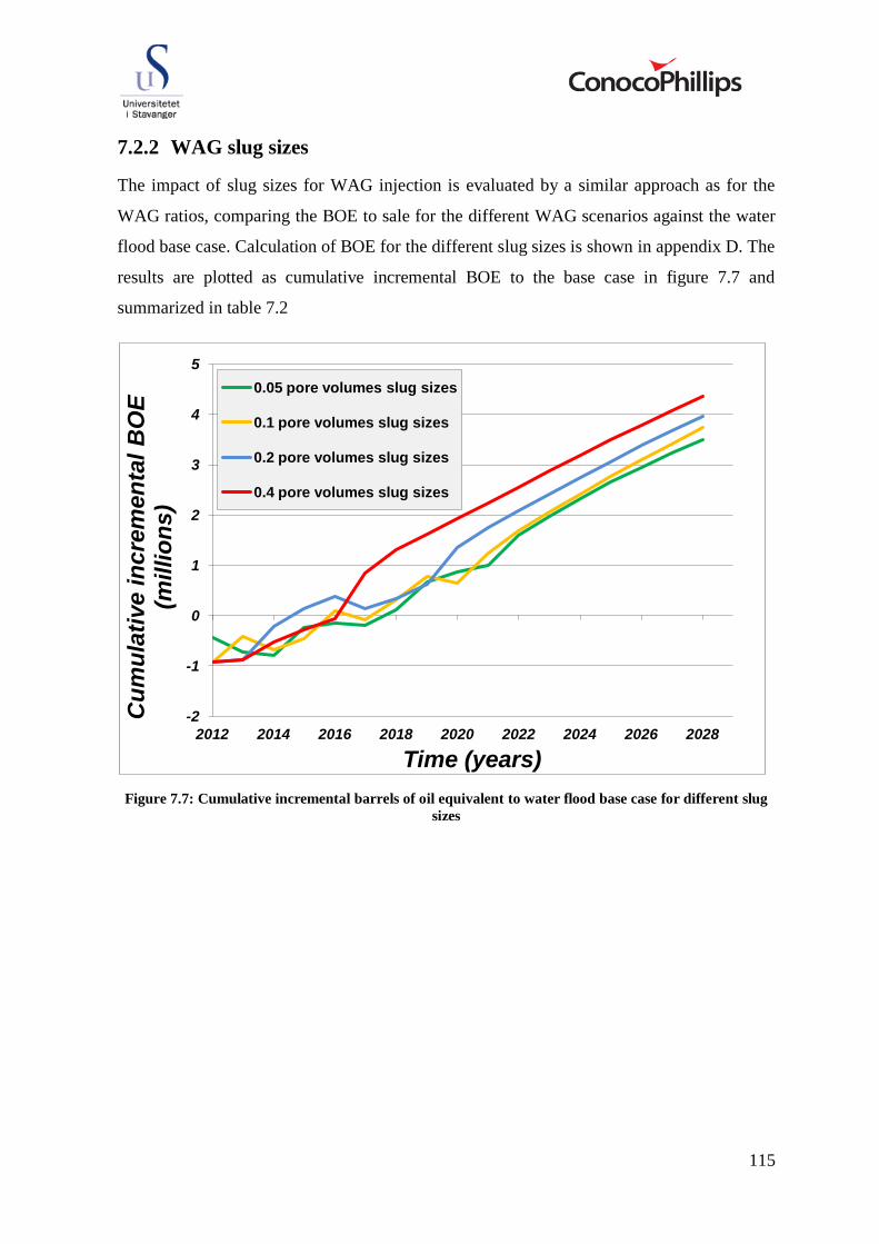
115
7.2.2 WAG slug sizes
The impact of slug sizes for WAG injection is evaluated by a similar approach as for the
WAG ratios, comparing the BOE to sale for the different WAG scenarios against the water
flood base case. Calculation of BOE for the different slug sizes is shown in appendix D. The
results are plotted as cumulative incremental BOE to the base case in figure 7.7 and
summarized in table 7.2
Figure 7.7: Cumulative incremental barrels of oil equivalent to water flood base case for different slug
sizes
-2
-1
0
1
2
3
4
5
2012 2014 2016 2018 2020 2022 2024 2026 2028
Cu
mu
lati
ve in
cre
men
tal
BO
E
(millio
ns)
Time (years)
0.05 pore volumes slug sizes
0.1 pore volumes slug sizes
0.2 pore volumes slug sizes
0.4 pore volumes slug sizes

116
Table 7.2: Barrels of oil equivalent and incremental barrels of oil equivalent to base case for different
slug sizes with WAG ratio 1:1 for the predictive part from 2011 to 2028
Scenario BOE to sale for
predictive period
(year 2011-2028)
Incremental BOE to
sale to the base case
Water flood
base case
17.5 million BOE -
0.05 pore volumes
half-cycle slugs
21.0 million BOE 3.5 million BOE
0.1 pore volumes
half-cycle slugs
21.2 million BOE 3.7 million BOE
0.2 pore volumes
half-cycle slugs
21.5 million BOE 4.0 million BOE
0.4 pore volumes
half-cycle slugs
21.9 million BOE 4.4 million BOE
Figure 7.7 and table 7.2 indicates that increasing the slug size results in increased oil
equivalent recovery. The best case was half-cycle slug size of 0.4 pore volumes which gave
an incremental 4.4 million BOE to the base case. It is observed that total gas injected of 0.4
pore volumes, give lower BOE than for same WAG ratio with total gas injected of 0.3 pore
volumes. Based on this result, the total volume of gas injected is recommended to be
investigated and optimized for further studies.
The coarse grid blocks of the sector model may lead to numerical dispersion when
implementing a WAG-injection, because of rapidly varying fluid fronts and large
differences in reservoir parameters between grid blocks. To avoid numerical dispersion and
instability problems caused by coarse gridding in WAG injection, local grid refinement can
be applied. The technique can improve grid resolution in particular areas of a model and
keep the coarse resolution in other areas. The option will minimize the number of grid
blocks and therefore reduce the CPU time of simulation compared to a regular grid
refinement option where grids in all areas are refined. The LGR methodology could be
useful around the WAG-injection well where fluid saturations change rapidly. The
technique is not used in this study because of its complexness, but is recommended to
include for further studies to avoid numerical dispersion.
117
8 Conclusion
The purpose of this thesis was to evaluate hydrocarbon WAG injection at the Ekofisk field.
Miscibility evaluation on MMP and MME, and modeling of important reservoir parameters
for WAG-displacement, such as trapped gas and hysteresis effect, matrix-fracture
mechanisms and SORM was suggested. Also modeling of WAG injection in a sector model
to optimize WAG ratios and WAG slug sizes, and to compare against a continuous water
flood case was suggested.
The evaluation was performed by running simulations in PSim for various models. The
following main conclusion can be drawn from the results from this study:
At current reservoir pressures at Ekofisk, WAG injection with dry hydrocarbon would
most likely be immiscible. This is based on the MMPs for dry hydrocarbon gas with the
Ekofisk crude oil determined in the range of 6600 to 7100 psia for different
temperatures.
The results showed that MME decreases with increasing pressures, which agrees with
theory. It was found that achieving miscibility by increasing the enrichment was not a
solution, because large amounts of NGL were needed. This involves high economical
risk because the relative high price NGL is delegated from sales to injection.
Mechanistic simulations on trapped gas showed that Lands trapped gas correlation with
input trapped gas value of 0.35 gave the best match to laboratory and reported trapped
gas data for chalks. It was also shown that neglecting trapped gas in simulations gives
optimistic predictions.
Simulations of different matrix-fracture systems gave significant differences in oil
recoveries and were used as an argument to introduce SORM for sector modeling, which
showed to be best described by the SORM Sotrig option.
WAG-scenarios in the sector model indicated incremental production to the water flood
base case for all cases. The best WAG ratio showed to be 1 to 2, with incremental
barrels of oil equivalent of 8.4 million to the base case. The incremental BOE decreased
118
with increasing WAG ratio. The optimized WAG slug sizes at WAG ratio of 1:1 showed
to be 0.4 pore volumes, with incremental BOE of 4.4 million to the base case.
Incremental BOE increased with increasing WAG slug sizes.
Recommendation for further work
It is recommended that further research be undertaken in the following areas:
Laboratory work on miscibility of dry hydrocarbon gas with the Ekofisk crude oil for
more accurate and reliable MMP evaluations.
More research on SORM and more accurate upscaling techniques from mechanistic
level to full field level.
Perform simulation work to investigate the total gas volume injected for WAG scenarios
in the sector model.
Introduction of local grid refinement to avoid numerical dispersion and instability
problems in the sector model.
Investigation of full field WAG potential by running full field simulations.
Economical study including aspects such as pipeline from production to injection
platforms, installation of compression pump, gas and NGL prices, sale of incremental oil
and net present value.

119
9 Abbreviations and symbols
BHP Bottom-hole pressure
BOE Barrels of oil equivalent
BWPD Barrels of water per day
CLand Lands trapping constant
C Trapping characteristics of porous rock
CPU Central processing unit
D Darcy, unit for permeability
EOR Enhanced oil recovery
EOS Equation of state
FCM First-contact miscibility
FI Fracture intensity factor
G Gravitational constant
GOR Gas to oil ratio
H Height of matrix blocks
HC-WAG Hydrocarbon water-alternating-gas
IFT Interfacial tension
k Absolute permeability
ke Effective permeability
kmat Matrix permeability from well log porosity or permeability correlations
kr Relative permeability
krg Relative permeability of gas
kro Relative permeability of gas
krog Relative permeability of oil in a gas-oil system
krow Relative permeability of oil in a water-oil system
krw Relative permeability of water
kwell Effect permeability from well tests
LGR Local grid refinement
LPG Liquefied petroleum gas
MCM Multi-contact miscibility
MME Minimum miscibility enrichment
MMP Minimum miscibility pressure

120
NGL Natural gas liquid
OOIP Original oil place
Pc Capillary pressure
Pnw Non-wetting phase pressure
PR-EOS Peng and Robinson equation of state
Psia Pounds per square inch, absolute pressure
PVT Pressure-volume-temperature
Pw Wetting-phase pressure
SCF/D Standard cubic feet gas per day
SCF/STB Standard cubic feet gas per standard oil barrel
Sg* Total gas saturation
SgF* Mobile fraction of gas
Sgi* Gas saturation at the start of imbibition process
Sgc Critical gas saturation
Sgr Residual gas saturation
Sgr* Residual trapped gas saturation after complete imbibition
Sgr*max Maximum obtainable residual gas saturation
Sgrc* Current trapped gas fraction of the gas
Som Mobile oil saturation
Sorg Residual oil to gas
SORM Miscible flood residual oil saturation
Sorw Residual oil to water
SorWAG Residual oil to WAG
STB/D Standard oil barrels per day
Swr Residual water saturation
WAG Water alternating gas
XG Fractional height of gas in the fracture
Xg Fractional height of the gas in the matrix
XWF Fractional height of water in the fracture
XWm Fractional height of the gas in the matrix
θ Contact angle
Empirically determined pore-size distribution factor
ρg Gas density

121
ρo Oil density
ρw Water density
σ Interfacial tension
σos Interfacial tension between solid and oil
σow Interfacial tension between water and oil
σws Interfacial tension between solid and water
φ Rock porosity

122
10 References
Agarwal, B., Thomas, L.K. and O'Meara, D.J. 1997. Reservoir Charcterization of
Ekofisk Field: A Giant, Fractured Chalk Reservoir in the Norwegian North Sea - Upscaling.
SPE 38875. October 1997.
Ahmed, T. 2000. Minimum Miscibility Pressure from EOS. Canadian International
Petroleum Conference. 4.-8. June 2000, Paper 2000-01.
Al-Wahaibi, Y.M, Muggeridge, A.H. and C.A.Grattioni. 2007. Experimental and
Numerical Studies of Gas/Oil Multicontact Miscible Displacements in Homogeneous and
Corssbedded porous Media. SPEJ 92887. March, 2007, page 62-76.
Al-Wahaibi, Yahya M. 2009. First-Contact-Miscible and Multicontact Miscible Gas
Injection within a Channeling Heterogeneity System. Energy&fuels article. 2009, Vol.
2010.
App, J.F. and Mohanty, K.K. 2002. The Benefit of Local Saturation Measurements in
Relative Permeability Estimation From Centrifuge Experiments. SPEJ September 2002.
2002, page 288-298.
Bark, E. Van den and O.D.Thomas. 1979. Ekofisk: First of the Giant Oil Fields in
Western Europe. s.l. : The American Association of Petroleum Geologists, 1979, page 195-
223.
Bernudez, L., Johns, R.T. and Parakh, H. 2007. Parametric Inverstigation of WAG
Floods Above the MME. SPEJ. June 2007, page 224-234.
Bradford, S.A. and Leij, F.J:. 1995. Wettability effect on scaling two- and three-fluid
capillary pressure-saturation relations. Env. Sci. Techn. 29, 1995, page 1446-1455.
Carlson, F.M. 1981. Simulation of Relative Permeability Hysteresis to the Nonwetting
Phase. SPE 10157. October 1981.
Christensen, J.R., Stenby, E.H and Skauge, A. 2001. Review of WAG Field Experience.
SPE 71203. April 2001, page 97-106.
Christian, T.M., et al. 1993. Reservoir Management at Ekofisk Field. SPE 26623. October
1993.
Clark, N.J., et al. 1958. Miscible Drive-Its Theory and Application. SPE 1036-G. June
1958.
ConocoPhillips Company (1). The Greater Ekofisk Area. [Internett] [Sitert: 04 April
2012.] http://www.conocophillips.no/EN/Norwegian%20shelf/Ekofisk/Pages/index.aspx.
123
ConocoPhillips Company (2). Worldwide operations: Norway. [Internett] [Sitert: 04 April
2012.]
http://www.conocophillips.com/EN/about/worldwide_ops/country/europe/pages/norway.asp
x.
ConocoPhillips Company (3). Discussion and presentations internally in ConocoPhillips.
2012
ConocoPhillips. January 1994. Ekofisk WAG Evaluation. Bartlesville : Phillips Petroleum
Company R&S Division, January 1994.
ConocoPhillips Keywords Manual. 2010. PSim Keywords Manual 2010.0. December
2010.
ConocoPhillips Technical Manual. 2010. PSim Technical Manual 2010.0. December
2010. pages 177-202, 140-148, 9-15
Conway, P.I., Damm, M. and Andersen, P.M. 1996. Full Field Dual Porosity Modelling
of a Complex Fractured Chalk Oil Reservoir Subject to Both Gas and Water Injection. SPE
36931. 22.-24. October 1996.
Dangerfield, J.A and Brown, D.A. 1987. The Ekofisk Field. [bokforf.] Graham Trotman.
The Norwegian Institute of Technology. 1987, page 3-22.
Donaldson, E.C., Thomas, R.D. and Lorenz, P.B. 1969. Wettability Determination and Its
Effect on Recovery Efficiency. SPEJ. March, 1969, page 13-20.
Dong, M., et al. 2005. Analysis of Immiscible Water-Alternating-Gas (WAG) Injection
Using Micromodel Tests. Journal of Canadian Petroleum Technology. February, 2005,
page 17-25.
Elsharkawy, A.M., Poettmann, F.H. and Christiansen, R.L. 1992. Measuring Minimum
Miscibility Pressure: Slim-Tube or Rising-Bubble Method? SPE/DOE 24114. 22-24 April
1992.
Faisal, A., et al. 2009. Injectivity and Gravity Segregation in WAG and SWAG Enhanced
Oil Recovery. SPE 124197. October 2009.
Firoozabadi, A. and Aziz, K. 1986. Relative permeability From Centrifuge Data. SPE
15059. 1986.
Goda, H. and Behrenbruch, P. 2011. A Universal Formulation for the Prediction Of
Capillary Pressure. SPE 147078. 2011.
Green, D.W. and Willhite, G. P. 1998. Enhanced Oil Recovery. Volume 6. 1998. 978-
1555630775. pages 12-27, 55-56, 190-196, 198-206
Hallenbeck, L.D, et al. 1989. Implementation of the Ekofisk Waterflood. SPE 19838. 1989.

124
Harpole, K.J., A.Østhus and Jensen, T.B. 2000. Screening for Ekofisk. SPE 65124.
October 2000.
Heeremans, J.C. and Kruijsdijk, C.P.J.W. van. 2006. Feasibility Study of WAG
Injection in Naturally Fractured Reservoirs. SPE 100034. 22.-26. April 2006.
Helland, J.O. and Skjæveland, S.M. 2004. Three-Phase Capillary Pressure Correlation for
Mixed-Wet Reservoirs. SPE 92057. November 2004.
Holm, L.W. 1987. Miscible Displacement. [bokforf.] Howard B. Bradley. Petroleum
Engineering Handbook. s.l. : Texas: Society of Petroleum Engineers., 1987, 45, ss. 1-9.
Hustad, O.S., et al. 2002. Gas Segregation During WAG Injection and the Importance of
Parameter Scaling in Three-Phase Models. SPE 75138. 13.-17. April 2002.
Ibrahim, M.N. Mohamad and Koederitz, L.F. 2001. Two-Phase Steady-State and
Unsteady-State Relative Permeability Prediction Models. SPE 68065. 2001.
Jakobsson, N.M. and Christian, T.M. 1994. Historical Performance of Gas Injection of
Ekofisk. SPE 28933. September 1994.
Jensen, T.B. 2001. Ekofisk Field - Simultaneous Water and Gas Injection- SWAG
Feasibility Study. Stavanger : Internal ConocoPhillips report, 2001.
Jethwa, D.J., Rothkopf, B.W. and Paulson, C.I. 2000. Successful Miscible Gas Injection
in a Mature U.K. North Sea Field. SPE 62990. 2000.
Jewhurst, J. and Wiborg, R. 1987. Ekofisk reservoir management in a compacting
environment. Sidney Australia : Internal ConocoPhillips report, 1987. page 54-67.
Johnson, J.P, Rhett, D.W. and Slemers, W.T. 1989. Rock Mechanics of the Ekofisk
Reservoir in the Evaluation of Subsidence. Journal of Petroleum Technology. July 1989,
page 717-722.
Kalam, Z., et al. 2011. Miscible Gas injection Tests in Carbonates and its Impact on Field
Development. SPE 148374. October 2011.
Keelan, Dare K. and J.Pugh, Virgil. 1975. Trapped-Gas Saturations in Carbonate
Formations. SPEJ. April 1975, page 149-160.
Killough, J.E. 1976. Reservoir Simulation With History-Dependent Saturation Functions.
SPEJ. February 1976, ss. 37-48.
Kleppe, Hans. 2011. Reservoir simulation course MPE750 at UiS, autumn 2011. University
of Stavanger : s.n., 2011. Chapter 6.

125
Kleppe, J., Teigland, R. and Awan, A.R. 2006. A Survey of North Sea Enhanced-Oil-
Recovery Projects Initiated During the Years 1975 to 2005. Revised SPE 99546. 2006, Vol.
2008, page 497-512.
Kossack, C.A. 2000. Comparison of Reservoir Simulation Hysteresis Options. SPE 63147.
October 2000.
Land, Carlon S. 1968. Calculation of Imbibition Relative Permeability for Two- and
Three-Phase Flow From Rock Properties. SPEJ. June 1968, page 149-156.
Land, Carlson S. 1971. Comparison of Calculated with Experimental Imbibition Relative
Permeability. SPE 3360. December 1971, page 419-425.
Larsen, J.A and Skauge, A. 1998. Methodology for Numerical Simulation With Cycle-
Dependent Relative Permeabilities. SPEJ. June 1998, page 163-173.
Larsen, J.A. and Skauge, A. 1995. Comparing hysteresis models for relative permeability
in WAG studies. SCA 9506. 1995.
Lekvam, Surgucchev and Ekrann. 1997. Hydrate Control for WAG injection in the
Ekofisk Field. Rogaland Research Institute, 1997. RF. 97/165.
Li, D., Kumar, K. and Mohanty, K.K. 2003. Compositional Simulation of WAG
Processes for a Viscous Oil. SPE 84074. 5.-8. October 2003.
Maloney, D.R. 2003. Consistency of Eldfisk, Ekofisk, and literature trapped gas results.
Upstream Reservoir Technology Report #17129. Bartlesville : ConocoPhillips, 2003.
Morrow, N.R. 1979. Interplay of capillary, viscous and buoyancy forces in the mobilization
of residual oil. Journal of Canadian Petroleum Technology (JCPT 79-03-03). July-
September, 1979.
Norsk Teknisk Museum. Det norske olje-eventyret 1965-2000. [Internett] [Sitert: 04 April
2012.] http://tekniskmuseum.no/gamlewebben/no/utstillingene/Jakten_oljen/historie.htm.
Pow, M., et al. 1997. Production of Gas From Tight Naturally-fractured Reservoirs With
Active Water. SPEJ 97-03. 1997. Annual Technical Meeting, Jun 8 - 11, 1997 , Calgary,
Alberta.
Ramachandran, K.P., Gyan, O.N. and Sur, S. 2010. Immiscible Hydrocarbon
WAG:Laboratory to Field. SPE 128848. 20.-22. January 2010.
Randall, T.E. and Bennion, D.B. 1988. Recent developments in slim tube testing for
hydrocarbon-miscible flood (HCMF) solvent design. Journal of Canadian Petroleum
Technology. Volume 27, No.6, November-December 1988, JCPT88-06-02, page 33-44.
126
Reservoir Laboratories AS. 1995. Tertiary gas injection following imbibition in a long
chalk sample. s.l. : ConocoPhillips in cooperation with Reservoir Laboratorias AS, as part of
"Ruth research program, WAG subprogram", 1995.
Sanchez, N.L. 1999. Management of Water Alternating Gas (WAG) Injection Projects. SPE
53714. 21.-23. April 1999.
Shyeh-Yung, J-G.J. 1991. Mechanisms of Miscible Oil recovery: Effect of Pressure and
Miscible and Near-Miscible Displacement of Oil by Carbon Dioxide. SPE 22651. 1991.
Skauge, A. and Dale, E.I. 2007. Progress in Immiscible WAG Modeling. SPE 111435.
October 2007.
Skauge, A. and J.A.Larsen. 1994. Three-phase relative permeabilities and trapped gas
measurements related to WAG processes. SCA 9421. September 1994, page 227-236.
Sohooli, Kh. 2012. Fracture Network Parameters in Dynamic Models of Fractured
Reservoir and Its Upscaling. SPE 151667. 20.-22. February 2012.
Spiteri, Elizabeth J. and Juanes, Ruben. 2004. Impact of Relative Permeability Hysteresis
on the Numerical Simulation of WAG injection. SPE 89921. September 2004.
Spronsen, E.V. 1982. Three-Phase Relative Permeability Measurements Using the
Centrifuge Method. SPE/DOE 10688. 1982.
Stone, H.L. 1970. Probability Model for Estimating Three-Phase Relative Permeability.
Journal of Petroleum Technology (2116). February 1970, ss. 214-218.
Stone, H.L. 1973. Estimation of Three-Phase Relative Permeability. Journal of Canadian
Petroleum Technology (JCPT73-04-06). October-December 1973, No.4, ss. 53-63.
Suicmez, V.S, Piri, M. and Blunt, M.J. 2006. Pore-Scale Modeling of Three-Phase WAG
injection: Prediction of Relative Permeabilities and Trapping for Different Displacement
Cycles. SPE 95594. April 2006.
Sulak, R.M. 1990. Ekofisk Field: The First 20 Years. SPE 20773. September 1990.
Sulak, R.M and Danielsen, J. 1989. Reservoir Aspects of Ekofisk Subsidence. Journal of
Petroleum Technology. July 1989, page 709-716.
Sylte, J.E, et al. 1999. Water Induced Compaction in the Ekofisk Field. SPE 56426.
October 1999.
Sylte, J.E, Hallenbeck, L.D. and Thomas, L.K. 1988. Ekofisk Formation Pilot
Waterflood. SPE 18276. October 1988.

127
Takla, L.A. and Sulak, R.M. 1989. Production Operations and Reservoir Aspets - Ekofisk
Area. October 1989. paper presented at the Integrated Petroleum Resource Management
Seminar and Workshop, Phillips, Stavanger, Norway.
Thomas, L.K, et al. 1987. Ekofisk Waterflood Pilot. Journal of Petroleum Technology.
February 1987, ss. 221-232.
Ursin, J.R. and Zolotukhin, A.B. 1997. Introduction to ResTek. Stavanger : UiS, 1997.
Pages 63, 67, 87-110, 115-118. Part of Reservoir Engineering Course BIP 140 autumn
2009.
Warren, J.E. and Root, P.J. 1963. The Behavior of Naturally Fractured Reservoirs. SPEJ
(SPE 426). September, 1963, page 245-255.
Wegener and Allred. 1997. Hydrate Formation Tendencies, Lean Gas, Water,
Thermodynamic Inhibitors. Predictions: Models versus Lab. Bartlesville : Phillips, 1997.
Presented Material.
Wegener, D.C and K.J.Harpole. 1996. Determination of Relative Permeability and
Trapped Gas Saturation for Predictions of WAG Performance in the South Cowden CO2
Flood. SPE 35429. April 1996, page 273-285.
Wu, R.S. and Batycky, J.P. 1990. Evaluation of miscibility from slim tube tests. The
Journal of Canadian Petroleum Technology. Volume 29, No.6, November-December 1990,
JCPT90-06-06, page 63-70.
Wu, X., et al. 2004. Critical Design Factors and Evaluation of Recovery Performance of
Miscible Displacement and WAG Process. Canadian International Petroleum Conference.
8.-10. June 2004, Paper 2004-192.
Zick, A.A. 1986. A Combined Condensing/Vaporizing Mechanism in the Displacement of
Oil by Enriched Gases. SPE 15493. October 1986.
Østhus, A. 1998. Ekofisk Whiskey WAG pilot. Stavanger : Internal ConocoPhillips report,
1998.
Øyno, Lars. 1995. Tertiary Gas injection Following Imbibition in a Long Chalk Sample.
Reservoir Laboratories AS. 1995. Report 344/10-96 for ConocoPhillips.

128
11 Appendices
Appendix A - Slim tube
MMP
268 F
Pressure Oil recovery at 1.2 PV gas
injected
3500 54,36
4000 57,72
4500 61,57
5000 66,48
5500 73,78
6000 81,32
6500 89,18
6800 94,26
6850 95,12
6900 95,84
6950 96,33
7000 96,67
7050 96,91
7100 97,11
7500 97,93
8000 98,43
9000 98,99
l re o er as a n t on o operat ng press re at F
200 F
Pressure Oil recovery at 1.2 PV gas
injected
3500 53,51
4500 60,99
5500 73,65
6000 80,79
6500 88,09
6900 94,35
7000 95,61
7100 96,26
7500 97,3
8000 97,83
l re o er as a n t on o operat ng press re at F
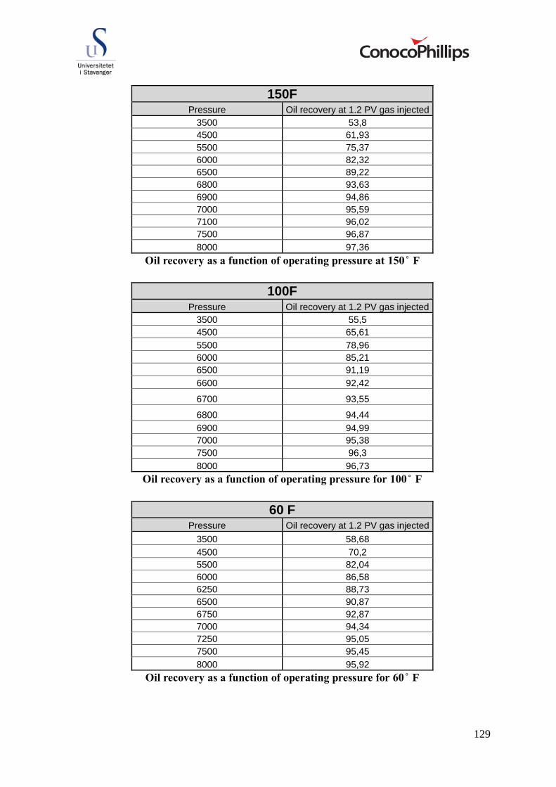
129
150F Pressure Oil recovery at 1.2 PV gas injected
3500 53,8
4500 61,93
5500 75,37
6000 82,32
6500 89,22
6800 93,63
6900 94,86
7000 95,59
7100 96,02
7500 96,87
8000 97,36
l re o er as a n t on o operat ng press re at F
100F Pressure Oil recovery at 1.2 PV gas injected
3500 55,5
4500 65,61
5500 78,96
6000 85,21
6500 91,19
6600 92,42
6700 93,55
6800 94,44
6900 94,99
7000 95,38
7500 96,3
8000 96,73
l re o er as a n t on o operat ng press re or F
60 F Pressure Oil recovery at 1.2 PV gas injected
3500 58,68
4500 70,2
5500 82,04
6000 86,58
6250 88,73
6500 90,87
6750 92,87
7000 94,34
7250 95,05
7500 95,45
8000 95,92
l re o er as a n t on o operat ng press re or F

130
MME
Total composition of injected gas with different degree of enrichment
268 F, 6000 psia Enrichment (NGL added) Oil recovery at 1.2 PV gas injected
0 % 81,32
2 % 82,56
5 % 85,6
8 % 90,25
10 % 93,43
12 % 95,82
15 % 97,72
20 % 99,47
l re o er as a n t on o enr ment le el at F and 6000 psia
268F, 5000 psia Enrichment (NGL added) Oil recovery at 1.2 PV gas injected
0 % 66,48
2 % 67,59
5 % 70,36
8 % 75,34
10 % 79,73
12 % 84,48
15 % 91,24
20 % 97,4
l re o er as a n t on o enr ment le el at F and 5000 psia

131
150 F, 6000 psia Enrichment (NGL added) Oil recovery at 1.2 PV gas injected
0 % 82,32
2 % 83,66
5 % 86,69
8 % 91,1
10 % 93,78
12 % 95,53
15 % 97,16
20 % 98,89
l re o er as a n t on o enr ment le el at F and 6000 psia
60 F, 6000 psia Enrichment (NGL added) Oil recovery at 1.2 PV gas injected
0 % 86,58
2 % 87,22
5 % 88,32
8 % 89,71
10 % 90,93
12 % 92,3
15 % 94,27
20 % 96,79
l re o er as a n t on o enr ment le el at F and 6000 psia

132
Appendix B – Test of EOS for immiscible conditions
Oil recovery from a slim-tube simulation for a 7-components EOS compared to a 15-
components EOS at operating pressure of 6500, which is close to miscible condition

133
Appendix C – trapped gas saturation and hysteresis effect
Oil saturation, gas saturation, pressure and oil saturation pressure as a function of
time in reference grid block (18,1,18) of the homogeneous matrix model for a run with
input trapped gas of 0.35

134
Oil saturation, gas saturation, pressure and oil saturation pressure as a function of
time in reference grid block (18,1,18) of the homogeneous matrix model for a run with
negligible trapped gas saturation

135
Appendix D – sector model
WAG-ratio
Calculation of BOE to sale for the WAG ratio 1:2 case
Calculation of BOE to sale for the WAG ratio 1:1 case

136
Calculation of BOE to sale for the WAG ratio 2:1 case
Calculation of BOE to sale for the WAG ratio 4:1 case

137
WAG slug sizes
Calculation of BOE to sale for the case of 0.05 pore volumes slug sizes
Calculation of BOE to sale for the case of 0.10 pore volumes slug sizes
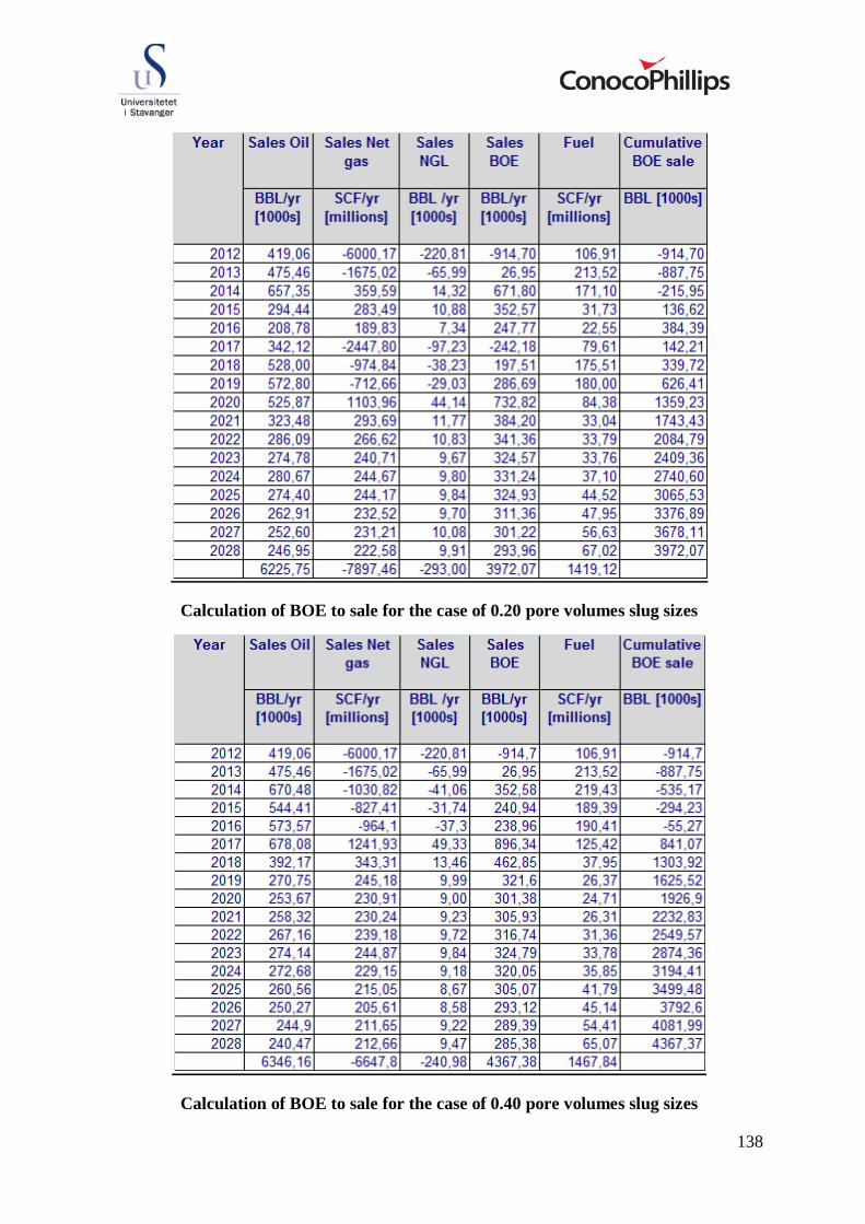
138
Calculation of BOE to sale for the case of 0.20 pore volumes slug sizes
Calculation of BOE to sale for the case of 0.40 pore volumes slug sizes