Embed Size (px)
Citation preview

Accepted Manuscript
Evenly spaced Detrended Fluctuation Analysis: Selecting the number ofpoints for the diffusion plot
Joshua J. Liddy, Jeffrey M. Haddad
PII: S0378-4371(17)30823-3DOI: http://dx.doi.org/10.1016/j.physa.2017.08.099Reference: PHYSA 18545
To appear in: Physica A
Received date : 1 April 2017Revised date : 3 July 2017
Please cite this article as: J.J. Liddy, J.M. Haddad, Evenly spaced Detrended Fluctuation Analysis:Selecting the number of points for the diffusion plot, Physica A (2017),http://dx.doi.org/10.1016/j.physa.2017.08.099
This is a PDF file of an unedited manuscript that has been accepted for publication. As a service toour customers we are providing this early version of the manuscript. The manuscript will undergocopyediting, typesetting, and review of the resulting proof before it is published in its final form.Please note that during the production process errors may be discovered which could affect thecontent, and all legal disclaimers that apply to the journal pertain.

1. We examined the performance of the evenly spaced Detrended Fluctuation Analysis
algorithms while manipulating the number of points in the diffusion plot, .
2. Simulated and experimental series of various lengths were analyzed.
3. Larger values of substantially reduce measurement uncertainty for single trials.
4. Between-trial means and standard deviations of α were less sensitive to .
5. We recommend maximizing based on series length to reduce measurement uncertainty.
*Highlights (for review)

Research Paper
Evenly Spaced Detrended Fluctuation Analysis: Selecting the Number of Points for the
Diffusion Plot
a Joshua J. Liddy &
a Jeffrey M. Haddad
a Department of Health and Kinesiology, Purdue University, West Lafayette, IN, USA, 47907
Correspondence
Joshua J. Liddy
Department of Health and Kinesiology
Purdue University
800 West Stadium Ave., West Lafayette, IN, USA, 47907
(978)-895-8091
Revised ManuscriptClick here to view linked References

1
Abstract
Detrended Fluctuation Analysis (DFA) has become a widely-used tool to examine the 2
correlation structure in a time series and provided insights into neuromuscular health and disease
states. As the popularity of utilizing DFA in the human behavioral sciences grows, understanding 4
its limitations and how to properly determine parameters has become increasingly important.
DFA examines the correlation structure of variability in a time series by computing , the slope 6
of the – diffusion plot. When using the traditional DFA algorithm, the timescales, ,
are often selected as a set of integers between a minimum and maximum length based on the 8
number of data points in the time series. This produces non-uniformly distributed values of in
logarithmic scale, which influences the estimation of α due to a disproportionate weighting of the 10
long-timescale regions of the diffusion plot. Recently, the evenly spaced DFA and evenly
spaced average DFA algorithms were introduced. Both algorithms compute by selecting 12
points for the diffusion plot based on the minimum and maximum timescales of interest and
improve the consistency of estimates for simulated fractional Gaussian noise and fractional 14
Brownian motion time series. Two issues that remain unaddressed are 1) how to select and 2)
whether the evenly-spaced DFA algorithms show similar benefits when assessing human 16
behavioral data. We manipulated and examined its effects on the accuracy, consistency, and
confidence limits of in simulated and experimental time series. We demonstrate that the 18
accuracy and consistency of are relatively unaffected by the selection of . However, the
confidence limits of narrow as increases, dramatically reducing measurement uncertainty for 20
single trials. We provide guidelines for selecting and discuss potential uses of the evenly
spaced DFA algorithms when assessing human behavioral data. 22
Keywords: Detrended Fluctuation Analysis, Even spacing, Diffusion Plot, Method Comparison,
Gait Variability 24

2
1. Introduction
Statistical techniques that examine the temporal structure of variability have become 2
increasing popular in the behavioral sciences. These methods have been used to assess serial
correlations in the variability of human physiological and behavioral processes including heart-4
rate [1-3], respiration [4, 5], blood flow [6-8], interpersonal coordination [9, 10], haptic
perceptual intent [11], visual search [12, 13], interlimb coordination [14-16], timing [17-19], 6
postural sway [20, 21], and gait [22-27]. Several reviews examining these techniques have
provided valuable guidelines regarding limitations, implementation, and interpretation [28-33]. 8
Detrended Fluctuation Analysis (DFA) [34] has emerged as one of the more robust and popular
statistical techniques for estimating the average correlation structure of a time series and has 10
provided insights into the underlying organization and control of human perception and action.
DFA exploits the diffusion property of fractional Brownian motion (fBm), which states 12
that the variance of a process, , is a power function of the timescale of observation, (Eq. 1).
(1) 14
Consequently, is characterized by a nonstationary mean and variance. The Hurst exponent, H,
determines the correlation structure of the fBm increments and is bounded on the interval . 16
= ½ corresponds to uncorrelated (random) increments. Persistent, or positively correlated,
increments are observed when > ½. Anti-persistent, or negatively correlated, increments are 18
present when < ½. Fractional Gaussian noise (fGn) represents a distinct family of stationary
processes formally related to fBm through summation and differencing. Specifically, cumulative 20
summation of fGn produces fBm, while differencing of fBm produces fGn. An important
characteristic of the dichotomous fGn/fBm framework [35] is that a fGn, , and its associated 22

3
fBm, , share the same value of . For fGn, determines the average correlation structure of
the signal, , rather than its increments. 2
DFA takes advantage of the formal relation between fGn and fBm and assesses a
derivation of the scaling relation in Eq. 1, stating that the standard deviation (SD) of an 4
integrated series, , is a power function of the timescale over which it is computed, , with
scaling exponent (Eq. 2). 6
(2)
The original series, , is classified as a fGn when is found on the interval and 8
consequently . If is on the interval , is considered a fBm and . The
scaling exponent therefore contains information regarding the classification (i.e., fGn vs. fBm) 10
and average correlation structure of the process under investigation.
The estimation of is determined by ordinary least-squares regression of on 12
(Fig. 1a). Several issues concerning the diffusion plot warrant attention. The selection of evenly
spaced timescales, , leads to a greater density of points in the long timescale region of the 14
diffusion plot following logarithmic transformation. The long-time scale region therefore has
greater influence because ordinary least-squares weighs observations equally. Autocorrelated and 16
heteroscedastic residuals are also commonly observed (Fig. 1d). Adherence to the basic
assumptions of Gauss-Markov Theorem guarantee that ordinary least squares coefficients are 18
unbiased and have minimum variance among all unbiased estimators [36]. Violations of
independence and homoscedasticity lead to inefficient estimation of the slope, or in the case of 20
DFA, which affects confidence limits. In practice, DFA is an unbiased estimator of for fGn
series, but underestimates fBm series [37, 38]. The biases observed for fBm series are related to 22
methodological assumptions inherent to DFA [37], specifically, the scaling relation in Eq. 2.

4
However, this assumption may be invalid when the original series is an fBm and the integrated
series, , belongs to a family of over-diffusive processes. 2
To improve the estimation of , Almurad and Delignières [38] formally introduced two
evenly spaced DFA algorithms to better select the timescales contained in the diffusion plot. The 4
evenly spaced DFA (esDFA) algorithm defines evenly spaced logarithmic timescales based on
the desired number of points in the diffusion plot, , and the minimum and maximum timescales 6
of interest, and [38]. The remaining -2 points are defined based on a geometric
progression. This algorithm selects an arbitrary set of timescales which may mask information 8
about the process under investigation if too few points are included in the diffusion plot. The
evenly spaced average DFA (esaDFA) algorithm incorporates timescales spanning to 10
by a common increment and defines intervals of equal width in logarithmic scale over which
estimates of and are averaged. Both evenly spaced algorithms reduce the influence of 12
longer timescales on the estimation of and improve the quality of the - regression
(Fig. 1d-f). As a result, the between-trial variability of is markedly lower for both evenly 14
spaced algorithms compared to DFA [38]. Another important benefit is that the evenly spaced
DFA algorithms exhibit the same between-trial variability for shorter time series (e.g., 16
points) as DFA does for longer time series (e.g., 1024 points) [38]. The ability to apply DFA to
shorter time series reduces the burdens associated with acquiring extended behavioral series, 18
which may be especially difficult to attain when working with special populations (e.g., children,
older adults, persons with neurological disorders). 20
Although the evenly spaced algorithms hold tremendous potential for the use of DFA, it
is important to address questions that emerge from the introduction of these algorithms. First, it 22
is unclear if the selection of influences estimates of . Almurad and Delignières [38] utilized

5
= 18, but it is unclear how this value was obtained. Presumably, the selection of should depend
on time series length. Because longer series contain a wider range of timescales, choosing too 2
few points may produce more volatile estimates of . Second, improvements to the quality of the
diffusion plot regression should narrow the confidence limits for . Confidence limits may 4
widen if residual variance is not substantially reduced because the evenly spaced DFA
algorithms include far fewer points than DFA. To our knowledge, confidence limits for α are not 6
reported even though many studies collect a single trial per experimental condition. Suggestions
to average α across trials to compensate for measurement variability have been made [37], but 8
adherence to this practice is not widespread. Reducing measurement uncertainty for individual
Fig. 1. Diffusion plots for (a) DFA, (b) esDFA, and (c) esaDFA algorithms for a fGn series of
1024 points with an expected of 0.7. Timescales ranged from 10 to /4. Similar to Almurad &
Delignieres (2016), = 18 was used for esDFA and esaDFA. and 95 % confidence limits are
displayed in the bottom right corner of panels a, b, and c. The bottom panels (e-f) display the
residuals of the linear, ordinary least-squares regression of log on log for (d) DFA, (e)
esDFA, and (f) esaDFA. Note the heteroscedasticity and residual autocorrelation in panel (d).
Both esDFA and esaDFA produce better behaved residuals despite slight heteroscedasticity (e)
and residual dependence (f). All R2 values exceeded 0.96.

6
trials is important when the experimental series are short or collecting multiple series is
impractical. Third, despite the improvements observed for large numbers of simulated time 2
series, no studies have systematically examined the benefits of the evenly-spaced DFA
algorithms when applied to human biophysical data. 4
The aims of this study were to determine 1) the influence of on the accuracy,
consistency, and uncertainty of and 2) the utility of the evenly spaced DFA algorithms for 6
assessing human movement data. The first aim was assessed using artificial fGn and fBm time
series. The second aim was addressed by examining locomotor variability in healthy adults 8
during treadmill walking and re-examining observations from a classic study of overground
walking [24]. 10
The selection of human locomotor variability is of both historical and practical relevance.
Early research by Hausdorff and colleagues identified the presence of long-term correlations in 12
human stride intervals and the degeneration of inter-stride correlations in aging and pathological
cohorts [23, 24, 39-41]. More recently, several researchers have pursued the utility of fractal, or 14
long-term correlated, auditory cues to enhance locomotor rehabilitation [42-45]. Gait variability
during treadmill locomotion consistently yields fGn series exhibiting statistical persistence for 16
stride time and length and anti-persistence for stride speed [25-27]. Overground stride interval
data collected by Hausdorff, Purdon, Peng, Ladin, Wei and Goldberger [24] exhibits a similar 18
range of behavior due to changes in walking speed and auditory cuing using an isochronous
metronome [22]. This allowed performance of the evenly spaced algorithms to be compared 20
among experimental series with different correlation structures.
22

7
2. Methods 2
2.1. Simulated Time Series
Simulated time series were generated using the Davies and Harte algorithm [46] which 4
produces fGn with an expected correlation structure determined by the Hurst exponent, . was
systematically varied from 0.1 to 0.9 in increments of 0.1. Simulated fGn time series were 6
generated for each value of . To produce fBm time series, a second set of fGn time series was
generated for each value of and cumulatively summed. The expected values of , denoted 8
from here on as , ranged from 0.1 to 1.9 in increments of 0.1 Given that the correlation
structure of fGn and fBm breaks down around , this value was excluded from the 10
simulations [47]. Series length, , was manipulated to produce simulations of 256, 512, and
1024 points. Simulations of different lengths were generated independently. 100 simulations 12
were produced for each combination of and .
2.2. Treadmill Walking 14
2.2.1. Participants
Fifteen healthy young adults (age = 20.0 ± 0.9 years, height = 170.0 ± 8.7 cm, weight = 16
70.2 ± 12.1 kg, 12 female) free of impairments affecting gait, participated in a one-day
assessment of treadmill walking. All participants provided written informed consent approved by 18
the university’s institutional review board.
2.2.2. Procedure 20
Participants walked at preferred walking speed for three five-minute trials on a 1.47 m
0.46 m treadmill (Life Fitness Inc., Rosemont, IL, USA). To determine preferred walking speed, 22
the speed of the treadmill belt was slowly accelerated and decelerated between 0.45 ms-1
and
1.79 ms-1
. Participants were instructed to inform the experimenter when preferred walking speed 24

8
was reached. Preferred walking speed was computed as the mean of the self-selected speeds
from a single increasing and decreasing ramp. Five-minutes of rest was given between trials. 2
2.2.3. Data Collection and Analysis
Kinematic data were collected at 120 Hz using a six-camera Vicon system (Vicon Motion 4
Systems, Oxford, UK). Two retro-reflective markers were placed on the head of the 2nd
phalanx
and the calcaneus of the right foot. Data were post-processed using MATLAB 8.6.0 (MathWorks 6
Inc., Natick, MA). Kinematic trajectories were low-pass filtered using a fourth order, dual-pass
Butterworth filter with a cutoff frequency of 10 Hz, similar to previous research [27]. Heel strike 8
events were estimated as the maximum anterior-posterior displacement of the heel [26, 27], and
were used to compute stride time ), stride length ( ), and stride speed ( ). was 10
defined as the time between ipsilateral heel strikes. To compute , the anterior-posterior
displacement of the heel between subsequent heel strikes was added to the product of treadmill 12
belt speed and . Each walking trial produced , , and series ranging from 259 to 292
strides depending on preferred walking speed. All series were subsequently reduced to the 14
middle 256 strides to control for series length.
To justify the sampling rate of 120 Hz, we resampled the kinematic trajectories to 40, 60, 16
240, and 360 Hz and computed α. On average, reducing the sampling rate to 40 or 60 Hz reduced
α estimates by 0.04 and 0.02, respectively. Lower sampling rates artificially introduced periods 18
of anti-persistent behavior, which reduced α, because of the limited temporal resolution.
Increasing the sampling rate to 240 Hz or 360 Hz increased mean estimates of α by 0.006 and 20
0.003, respectively. More deliberate exploration of the effects of filtering and sampling during
rhythmic movements (e.g., timing, locomotion, bimanual coordination) may aid in establishing 22
acquisition and processing guidelines prior to submitting these data to DFA.

9
2.3. Overground Walking
Stride intervals data from Hausdorff, Purdon, Peng, Ladin, Wei and Goldberger [24] 2
(made available at https://physionet.org/physiobank/database/umwdb/) were reanalyzed. Data
were collected from 10 healthy male adults (mean age 21.7 years; range 18-29 years). 4
Participants performed overground walking on either a 225 m or 400 m oval track. Stride
intervals were estimated using force-sensitive footswitches inserted beneath a single foot. Two 6
walking conditions were included: free-walking at self-selected (normal) pace for 1 h and
metronomic walking at normal pace for 0.5 h. During the metronomic conditions, participants 8
were instructed to synchronize their heel strike with the sounding of an isochronous metronome.
The metronome period was set to the mean stride interval from the normal free-walking 10
condition. Stride interval time series, also referred to as , ranged from 2977 - 3822 strides for
the free-walking conditions and 1439 - 1798 strides for the metronomic walking conditions. To 12
facilitate comparisons to the simulated and treadmill walking series, each series was reduced
to the middle 256, 512, and 1024 strides. 14
2.4. Detrended Fluctuation Analysis
The procedures for the evenly spaced DFA algorithms are similar to DFA with the 16
exception of the number of points contained in the diffusion plot All three procedures are
explained below. The timescales for all three algorithms ranged from = 10 to = /4. 18
2.4.1. DFA
To estimate the scaling exponent, , in Eq. 2, a series of length is integrated (Eq. 3). 20

10
is then divided into 1 non-overlapping intervals of length, . The integrated series is
locally detrended by fitting an order polynomial to each interval using least-squares 2
approximation and subtracting the fitted values from . This study used first order
detrending, i.e. = 1. Next, the mean square error (MSE) of the detrended interval is computed. 4
MSE is estimated for all intervals of timescale . The MSE values are then averaged and the
square root of the resulting value is computed to determine (Eq. 4). 6
This procedure is repeated for all timescales. Timescales, , ranged from 10 to /4 by 1. Given 8
the expectation of power-law scaling between and , is estimated as the slope of the linear,
ordinary least-squares regression of on . 10
2.4.2. Evenly Spaced DFA
The procedure for esDFA is identical to DFA (Eq. 4). The innovation of esDFA is the 12
selection of the timescales, . Values of are selected by specifying lower and upper limits,
and , and the number of timescales included in the diffusion plot, ( ). 14
Timescales were defined based on Eq. 6 [38].
2 (5) 16
1 denotes the floor function.
2 denotes the round function.

11
2.4.3. Evenly Spaced Average DFA
Similarly, esaDFA generates points for the diffusion plot prior to estimating . The 2
procedure is initially identical to DFA. is computed for ranging from to by
1. Before estimating , the range of is divided into intervals of equal width in logarithmic 4
scale. Each interval in logarithmic scale is specified by:
6
for . The corresponding intervals in timescale are determined by:
8
for [38]. The average timescale and , and are computed within each
interval, producing points. Unlike esDFA, each estimate of potentially contains 10
information from multiple estimates of within .
2.5. Number of Points in the Diffusion Plot, 12
The esDFA algorithm selects points for the diffusion plot based on the minimum, ,
and maximum, , timescales. The -2 remaining points, , are determined by Eq. 5. Since 14
values of must be integers, values of are rounded. This procedure is problematic if is large
relative to the range spanned by and . Based on the procedure outlined in Eq. 5, two 16
values of can be rounded to the same integer. If this occurs, the diffusion plot will contain
fewer than points. 18
A similar problem is encountered with the esaDFA algorithm. esaDFA computes
for all values of from to . In this study, values of ranged from 10 to /4 by 1. The 20
values of are divided into non-overlapping intervals which are evenly-spaced in logarithmic
scale. When is small, intervals will contain at least one value of . As increases, interval 22

12
widths shrink and may not include any values of . The diffusion plot will therefore contain
fewer than k points because and are not estimated for some intervals. 2
Two solutions are proposed. First, the non-unique values of or empty intervals can be
omitted from the regression, but this results in fewer than points. Second, the maximum value 4
of , for which all are unique or no intervals are empty can be computed. For esDFA,
can be determined by selecting , , and k, and computing the evenly spaced values 6
of using Eq. 5, while ensuring that all values of are unique. This procedure is repeated for
increasing values of until the criterion above is violated. For esaDFA, a similar procedure can 8
be implemented by selecting values of , , and , computing interval bounds using Eq.
7, and ensuring that all intervals contain at least one value of . If no intervals are empty, the 10
procedure is repeated for increasing values of until an empty interval is found.
was estimated using the algorithms described above while varying from 128 to 12
2048. The minimum and maxim timescales, and , were fixed at 10 and /4,
respectively. Two distinct functions of were identified for esDFA and esaDFA (Fig. 2). On 14
average, increases logarithmically for both algorithms, but is greater for esDFA. The
intermittent drops observed in the esDFA function are attributed to the rounding procedure. 16
To simplify parameterization for researchers interested in using the evenly-spaced
algorithms, we have included supplemental materials that provide guidelines for selecting k (see 18
Supplementary Materials). The levels of examined in this study were selected to afford
comparisons between the evenly spaced algorithms. For series of 256, 512, and 1024 points, 20
is 27, 37, and 47, respectively. Since varies with , we examined different values of
for series of 256, 512, and 1024 points. The minimum value of was selected as 10 22

13
independent of series length. Values of were selected to be 25, 35, and 45 for series of 256,
512, and 1024 points, respectively. Values of k ranged from 10 to by 5. 2
4 2.6. Statistical Analysis
and 95 % confidence limits of were computed for the simulated and experimental 6
time series. The width of the confidence limits, , provide an indication of the measurement
uncertainty of within trials. Confidence limits for were computed as: 8
where , , and represent the number points in the diffusion plot, , and , 10
respectively. was computed as the difference between the upper and lower bounds of the
confidence limits. For the simulated series, accuracy, consistency, and uncertainty were assessed 12
by computing the mean and standard deviation of α, and the mean of across 100 simulations
for each level of , k, and N. For the treadmill walking series, the mean and standard 14
Fig. 2. The maximum number of points in the diffusion plot, , for a
series of length with =10 and = /4 for esDFA (black curve)
and esaDFA (red curve).

14
deviation of and the mean of were computed for , , and within and then across
subjects for each level of k. For the overground series, which consist of a single trial per subject, 2
the mean of and were computed across subjects for for each level of k and N. Accuracy
is not discussed in the context of the experimental series due to the lack of an expected value or 4
gold-standard for assessing α.
3. Results 6
3.1. Simulated fGn and fBm Series
3.1.1. Effect of k on Accuracy 8
Fig. 3 illustrates the accuracy of for the simulated fGn and fBm series. Since the
estimation of does not depend on for DFA, a single estimate was produced for each 10
combination of and . The accuracy of for the simulated series is independent of .
Similar to previous findings, DFA produces unbiased estimates of for the fGn series and 12
slightly underestimates for the fBm series [37, 38]. This is particularly evident in shorter series
with 1.1 1.3. No differences in the accuracy of were observed between algorithms, 14
confirming the findings of Almurad and Delignières [38].
3.1.2. Effect of k on Consistency 16
The consistency of α for the simulated series is presented in Fig. 4. In general, the
standard deviation of increases with for the fGn series. For the fBm series, the variability 18
of rises as increases, leveling off around 1.5. The esaDFA algorithm was relatively
unaffected by k, while esDFA exhibited greater variability for small k. For series of 256 and 512 20
points, esDFA yielded slightly more consistent estimates. Both algorithms performed similarly
for series of 1024 points independent of k. Consistency improved systematically with increased 22
series length. Both evenly spaced algorithms produced more consistent estimates compared to

15
DFA (Fig. 5). The magnitude of these improvements reported in Almurad and Delignières [38]
were approximately 35 %. Our results demonstrate that improvements in consistency depend on 2
and N. Consistency improved on average by approximately 10 %, 15 %, and 25 % for
series of 256, 512, and 1024 points, respectively. On average, esDFA showed marginally higher 4
consistency than esaDFA.
Fig. 3. Mean estimates of versus for DFA (left panels), esDFA (middle panels), and
esaDFA (right panels) for each series length. The solid black lines represent the line of identity.
Separate curves are shown for the evenly-spaced algorithms for each value of . Curves for each
value of k are superimposed due to the small differences between α estimates.

16
3.1.3. Effect of k on Uncertainty
Fig. 4. Standard deviations of versus for DFA (left panels), esDFA (middle panels), and
esaDFA (right panels) for each series length. Separate curves are shown for the evenly-spaced
algorithms for each value of , but may be superimposed.

17
The average width of the 95 % confidence limits for , , are shown in Fig. 6. Because
confidence limits for are infrequently computed in the literature, it is worth noting changes to 2
for DFA. For the fGn series, increases linearly with , but the rate of increase
decreased for longer series. Confidence limits were wider for the fBm series and elevated 4
between 1.3 1.7. For fBm series of 256 points, rises to nearly 0.2. Increasing series
length reduced to values of 0.05 or lower for all . 6
For the evenly spaced algorithms, the selection of substantially affects . As k
increases, the confidence limits narrow. The greatest improvements in the fGn series are 8
observed as approaches 1/f noise and in the fBm series as approaches a random walk (i.e., α
= 1.5). The esDFA algorithm is more sensitive to , particularly for short series. For large , the 10
esDFA confidence limits are wider than both DFA and esaDFA. With increasing series length,
esDFA estimates of become comparable. esaDFA shows comparable performance to DFA 12
Fig. 5. Percent differences of the standard deviation of α for esDFA (top panels) and esaDFA
(bottom panels) with respect to DFA. Both evenly spaced algorithms produce more consistent
estimates of α and improvements were greater for longer series. Means ± standard deviations
across values of k and α are displayed in each panel.

18
for large k despite containing substantially fewer points in the diffusion plot. The selection of k is
therefore critical for reducing measurement uncertainty in single trials. 2
3.2. Treadmill Walking
3.2.1. Effect of k on Means 4
Fig. 6. Means of versus for DFA (left panels), esDFA (middle panels), and esaDFA
(right panels) for each series length. Separate curves are shown for the evenly-spaced algorithms
for each value of , which depends on series length.

19
Mean estimates of for , , and across subjects are displayed in Fig 7. Compared
to DFA, the evenly spaced algorithms often produced lower estimates for and and higher 2
estimates for . Between-method differences were consistently small (0.01 – 0.03) and did not
depend on . The relatively small differences observed between algorithms and levels of k are 4
congruent with the results from the simulated series.
3.2.2. Effect of k on Consistency 6
Fig. 8 displays the consistency of α for , , and during treadmill walking. The
standard deviation of was computed within and then between subjects. Differences between 8
algorithms therefore represent average differences in the consistency of α. For and series,
both evenly spaced algorithms produced more consistent estimates by approximately 10-20 % 10
compared to DFA. Similar to the results obtained from the simulated series, esDFA was more
slightly more consistent than esaDFA. Both algorithms produced more variable estimates 12
compared to DFA. No effect of was observed. Based on Fig. 4, fGn series with anti-persistent
Fig. 7. Mean estimates of for , , and for (a) esDFA and (b) esaDFA at different values
of . Estimates computed using DFA are represented by the dashed horizontal lines.

20
structure (i.e., ) are expected yield more consistent measurements than series with persistent
structure (i.e., and ). Fig 8. demonstrates that the between-trial variability for is 2
approximately half the magnitude of and , which closely reflects the expected differences.
3.2.3. Effect of k on Uncertainty 4
Mean estimates of for , , and are shown in Fig. 9. were averaged within
and then between subjects. The evenly spaced algorithms produce wider confidence limits for , 6
Fig. 8. Standard deviations of for , , and for (a) esDFA and (b) esaDFA at different
values of . Estimates computed using DFA are represented by the dashed horizontal lines.
Fig. 9. Confidence limits of for , , and for (a) esDFA and (b) esaDFA at different
values of . Estimates computed using DFA are represented by the dashed horizontal lines.

21
, and compared to DFA. As expected, was wider for persistent fGn series (i.e., and
) than anti-persistent series (i.e., ). Notably, reduced dramatically as increased. For 2
small , is unacceptably large, reaching nearly 0.25 for and . esaDFA consistently
produced narrower confidence limits than esDFA. Mean differences between the evenly spaced 4
algorithms and DFA were greater for persistent series (i.e., and ).
3.3. Overground Walking 6
3.3.1. Effect of k on Means
Fig. 10 displays mean estimates of for . During the free-walking condition, the 8
evenly spaced algorithms underestimated relative to DFA for short series. By contrast, was
overestimated during metronomic walking (range: 0.02 – 0.05). Mean estimates of were 10
insensitive to k, similar to the simulated and treadmill walking series. The differences between
Fig 10. Mean estimates of for for DFA, esDFA, esaDFA at each level of . Normal free-
walking and metronomic walking are presented in the top and bottom panels, respectively, for
each series length.
22
the three algorithms decreased for long series in the free-walking condition. The largest
differences between the evenly spaced algorithms and DFA was observed during the metronomic 2
walking condition for series of 512 points.
3.3.2. Effect of k on Uncertainty 4
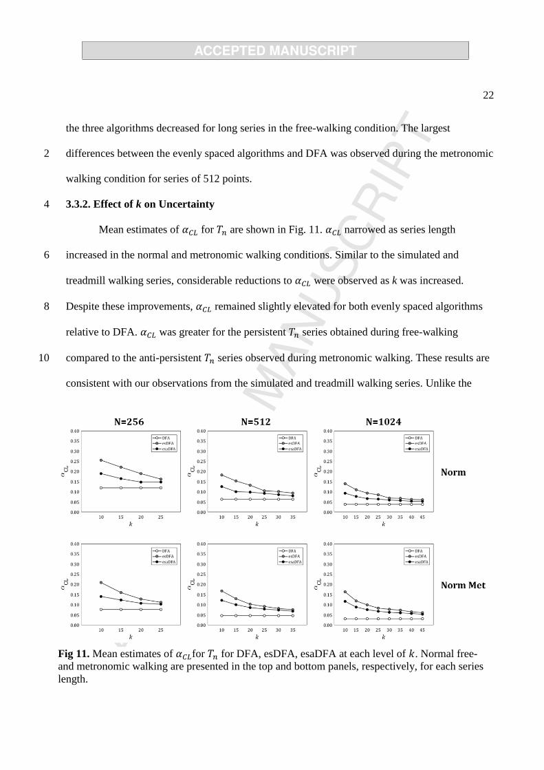
Mean estimates of for are shown in Fig. 11. narrowed as series length
increased in the normal and metronomic walking conditions. Similar to the simulated and 6
treadmill walking series, considerable reductions to were observed as k was increased.
Despite these improvements, remained slightly elevated for both evenly spaced algorithms 8
relative to DFA. was greater for the persistent series obtained during free-walking
compared to the anti-persistent series observed during metronomic walking. These results are 10
consistent with our observations from the simulated and treadmill walking series. Unlike the
Fig 11. Mean estimates of for for DFA, esDFA, esaDFA at each level of . Normal free-
and metronomic walking are presented in the top and bottom panels, respectively, for each series
length.

23
treadmill walking data, clear differences between esDFA and esaDFA were observed, especially
for small k. These differences decreased as k increased. 2
4. Discussion
Guidelines for selecting the number of data points in the diffusion plot, k, for the evenly 4
spaced DFA algorithms were previously unaddressed. We demonstrate that the selection of has
marginal impact on the accuracy and consistency of for simulated and experimental series. 6
However, the most notable contributions of this study are the introduction of confidence limits to
quantify measurement uncertainty for single trials and the significant reductions to the 8
confidence limits of α observed for large values of k. The selection of k requires careful
consideration and is strongly tied to the length of the experimental series and timescales of 10
interest. Below we discuss the implications of our findings, considerations for parameterization,
and potential applications for the evenly spaced DFA algorithms. 12
We begin by discussing the implications of our results as they relate to the accuracy and
consistency of α, which was previously explored by Almurad and Delignières [38]. The accuracy 14
of α is predominantly affected by the classification and correlation structure the analyzed series,
but not by k. DFA commonly produces under-additive estimates of for fBm series [28, 37, 38]. 16
That is, when a fGn series with an expected value of = is cumulatively summed, the estimate
of is commonly less than the expected value of = . The results presented here 18
corroborate observations that DFA underestimates α for fBm. The evenly spaced algorithms are
equally susceptible to these errors. To combat these issues, several research groups have 20
suggested a preprocessing step of classifying time series as a fGn or fBm [28, 29, 37]. When an
experimental series is identified as a fBm, the integration procedure may be omitted thereby 22

24
producing unbiased estimations of . Estimating with confidence limits on a trial-by-trial basis
may therefore facilitate more robust classification of behavioral data. 2
Both evenly spaced DFA algorithms improve the consistency of α estimates for simulated
and experimental series, confirming the findings of Almurad and Delignières [38]. The 4
improvements to measurement variability observed in this study were substantially lower,
ranging from 10 % to 25 %, depending on series length. The source of this discrepancy is related 6
to the timescales included in the analysis. Almurad and Delignières [38] used = 10 and
= N/2. In the current study, we set to N/4. To substantiate the improvements to 8
consistency reported by Almurad and Delignières [38], we reanalyzed the simulated fGn and
Fig. 12. Percent differences of the standard deviation of α for esDFA (top panels) and esaDFA
(bottom panels) with respect to DFA. Red dashed lines represent the 35 % improvements to
consistency reported in Almurad and Delignieres [38]. and were set to 10 and N/2,
respectively. Means ± standard deviations across values of k and α are displayed in each panel.

25
fBm series and set to N/2. The range of k values was consistent with the original analysis
(i.e., 10 to 25, 35, or 45 by 5). The results obtained from these analyses are displayed in Fig. 12. 2
Both evenly spaced algorithms showed greater consistency compared to DFA. These
improvements increased for longer series. The esaDFA algorithm produced more consistent 4
estimates compared to esDFA, particularly for longer series. Thus, similar improvements in
measurement consistency, as reported in Almurad and Delignières [38], was achieved by setting 6
to N/2. Furthermore, increasing will increase . While we did not explore
increasing k beyond the values used in this study, further decreases to the confidence limits of α 8
can be expected as k increases. Based on the reanalysis described above, the selection of
has considerable influence on measurement consistency and should be selected carefully. 10
Recommendations for as low as N/9 have been proposed in the literature [48]. However,
for short series, e.g. 256 data points, the maximum timescale would be a mere 28 points. We 12
used to a maximum timescale of N/4 to 1) incorporate a wider range of timescales in the analysis
and 2) to increase the number of intervals included in the computation of at longer 14
timescales. However, we recommend setting to N/2 when using the evenly spaced
algorithms to improve consistency across estimates. 16
To our knowledge, this is the first study to compute confidence limits for α. As
mentioned above, computing confidence limits may facilitate better classification of single 18
behavioral series (e.g., fGn versus fBm or anti-persistent versus persistent). The quality of the
– regression is often assessed by examining the diffusion plot or R2 values. The 20
importance of visually inspecting the diffusion plot before applying DFA cannot be overstated.
Identifying the presence of multiple scaling regions or a nonlinear relationship between – 22
is important for determining whether DFA is appropriate. However, even when the

26
diffusion plot contains a linear trend, the measurement uncertainty of α may be large. We
observed that larger k values substantially reduce single trial measurement uncertainty. This was 2
particularly evident for longer time series (e.g., 1024 points). Reductions to for longer series
are related to two factors. First, the number of points in the diffusion plot determines the degrees 4
of freedom for selecting the t-score (i.e., ). The t-distribution is leptokurtic (i.e., exhibits
excess positive kurtosis), approaching the normal distribution as the degrees of freedom, -2, 6
increases, which decreases the associated t-score. Second, the standard error of depends on ,
the mean square error, and the sum of the squared values of . The standard error decreases 8
when is large. Thus, measurement uncertainty reduces as a function of including more points
in the diffusion plot. 10
Increasing k to values near may not always be optimal. Both evenly spaced
algorithms require the number of points in the diffusion plot, , to be specified in advance. We 12
showed that the maximum value of depends on timescales of interest and which algorithm is
being used (see Section 2.5 and Supplemental Materials). The esDFA algorithm has slightly 14
higher limits for compared to esaDFA. It should be noted that esDFA selects points which
would normally be contained in the DFA diffusion plot. As increases, heteroscedasticity and 16
autocorrelated residuals will reemerge. Given that esDFA incorporates significantly fewer points
than DFA, the confidence limits of α will widen, increasing the uncertainty of each estimate. To 18
explore the effect of increasing beyond the range examined in this study, esDFA was reapplied
to the simulated fGn and fBm series for values ranging from 10 to 30, 40, or 55 by 5 for series 20
of 256, 512, and 1024 points, respectively. These values were selected based on their proximity
to . The accuracy of was unchanged by further increases to . The consistency of was 22
similar between small and large values of . The most consistent estimates were observed for

27
moderate values of k. The width of the confidence limits narrow as is increased, but
improvements saturate for longer series and large values of k. Thus, increasing beyond the 2
limits examined in this study counteracts a major benefit of esDFA, namely better consistency
across estimates. Tradeoffs between maximizing consistency across estimates and minimizing 4
the uncertainty of single estimates are therefore unavoidable when using esDFA. We recommend
careful examination of the effect of on estimates of be incorporated into preprocessing 6
procedures if the esDFA algorithm is used.
Almurad and Delignières [38] hypothesized that the esaDFA algorithm should 8
outperform esDFA based on the observation that the points included in the diffusion plot
potentially contain information from multiple timescales, thereby averaging out local 10
fluctuations of . Our findings confirm their intuition to an extent. The evenly spaced
algorithms are comparable in terms of accuracy. However, esaDFA produces more consistent 12
estimates across trials, especially for longer series, and narrower confidence limits for single
trials. Overall, esaDFA is preferable to esDFA based on the simulated and experimental time 14
series analyzed in this study.
To address the second aim of the study, we examined the performance of the evenly 16
spaced DFA algorithms using experimental time series of human locomotor variability. Unlike
the simulated time series, no reference value for assessing the accuracy of exists for the 18
experimental series. We therefore limited our comparisons to estimates produced by DFA. All
experimental series examined in this study were classified as fGn. The evenly spaced algorithms 20
slightly underestimated α for persistent series and slightly overestimated α for anti-persistent
series compared to DFA. These results were observed for treadmill and overground walking and 22
may indicate that DFA overestimates the degree of persistence or anti-persistence. Conversely,

28
the evenly spaced algorithms may provide more conservative estimates of the correlation
structure of fGn series. The evenly spaced algorithms provide similar or better consistency across 2
estimates from the same subject. However, measurement uncertainty for single trials was slightly
elevated compared to DFA for both treadmill and overground walking, but can be combatted by 4
adjusting and k accordingly (see below). Overall, the benefits of the evenly spaced DFA
algorithms were similar between synthetic fGn series and experimental series of human 6
locomotor variability.
The advantages of improved consistency across measurements and reduced uncertainty 8
within measurements is beneficial to behavioral researchers, particularly those in clinical settings
where patient interaction is time-sensitive. If relatively few trials are collected, especially for 10
short series, we recommend setting to N/2 and increasing k to when using esaDFA
because it will improve consistency across trials and reduce uncertainty within trials. If 12
individual trials are leveraged to increase the degrees of freedom in a statistical analysis, these
parameter values will safeguard against unacceptably large confidence limits which may render 14
individual estimates of meaningless.
In response to a point raised by Almurad and Delignières [38] regarding the utility of 16
even spacing for the detection of crossover phenomena (e.g., Delignieres, Torre and Bernard
[20], Collins and De Luca [21]), the identification of a crossover point would presumably be best 18
served by increasing the number of points in the diffusion plot to a value near to improve
the resolution of the diffusion plot. Crossovers are particular problematic, especially if the series 20
under investigation exhibits quasiperiodic trends [49]. However, if a crossover is observed due to
the clear presence of a single periodic trend, the timescale at which the scaling behavior changes 22
may contain important information. Crossovers in postural sway have been interpreted as a

29
bounding of center-of-pressure velocity based on observations of persistent short-term and anti-
persistent long-term dynamics [20]. These observations are consistent with notions of boundary-2
relevant postural stability [50-52] and intermittency [53-55]. Shifting of the crossover point may
reflect changes to open- and closed-loop regulation of posture, possibly as a function of changing 4
performance demands. The timescales contained in each scaling region would presumably
depend on the implications of postural variability on the maintenance of stance and concurrent 6
behavioral goals. For example, increasing the precision demands of a concurrent manual task
while standing requires greater vigilance of extraneous postural fluctuations. Postural sway 8
might therefore be corrected more frequently, thereby shifting the crossover point to shorter
timescales. Unfortunately, crossover phenomena in postural sway present major difficulties 10
because the presence of distinct scaling regions strongly depends on the sampling rate and the
timescales included in the analysis [53]. Future inquiries into these phenomena may be facilitated 12
by employing the evenly spaced algorithms and objective methods for identifying the crossover
point [56]. 14
5. Conclusion
The results of this study, combined with the findings of Almurad and Delignières [38], 16
provide support for adoption of even spacing when applying DFA. While several contemporary
studies have utilized even spacing, the evenly spaced DFA algorithms represent a significant 18
improvement for estimating the correlation structure of behavioral time series. In general,
esaDFA is preferable to esDFA due to improved consistency across trials and reduced 20
measurement uncertainty within trials. The number of points in the diffusion plot is primarily
affects the uncertainty of within a trial. Increasing dramatically narrows the confidence 22
limits of , which may be particularly relevant in experimental settings when single trials are

30
collected. The benefits observed for simulated series transfer to behavioral series, specifically
gait variability, but further exploration of the applicability of the evenly spaced DFA algorithms 2
to behavioral data is warranted. We therefore encourage researchers to examine the efficacy and
limitations of these techniques in other domains. 4

35
Acknowledgments
None.

36
Funding Source
This work was supported by the Indiana Clinical and Translational Science Institute (Grant
UL1TR001108) and the National Science Foundation Dynamical Systems Program (Grant
CMMI-1300632). These funding sources had no role in the study design, data collection or
analysis, interpretation of the results, or decision to submit this research.

37
Conflicts of Interest
The authors declare no conflicts of interest.

38
References
[1] T.H. Mäkikallio, S. Høiber, L. Køber, C. Torp-Pedersen, C.K. Peng, A.L. Goldberger, H.V.
Huikuri, Fractal analysis of heart rate dynamics as a predictor of mortality in patients
with depressed left ventricular function after acute myocardial infarction, Am J Cardiol,
83 (1999) 836-839.
[2] C.K. Peng, S. Havlin, J.M. Hausdorff, J.E. Mietus, H.E. Stanley, A.L. Goldberger, Fractal
mechanisms and heart rate dynamics. Long-range correlations and their breakdown with
disease, J Electrocardiol, 28 Suppl (1995) 59-65.
[3] J.M. Tapanainen, P.E. Thomsen, L. Kober, C. Torp-Pedersen, T.H. Makikallio, A.M. Still,
K.S. Lindgren, H.V. Huikuri, Fractal analysis of heart rate variability and mortality after
an acute myocardial infarction, Am J Cardiol, 90 (2002) 347-352.
[4] C.K. Peng, J.E. Mietus, Y. Liu, C. Lee, J.M. Hausdorff, H.E. Stanley, A.L. Goldberger,
L.A. Lipsitz, Quantifying fractal dynamics of human respiration: age and gender
effects, Ann Biomed Eng, 30 (2002) 683-692.
[5] P.J. Fadel, S.M. Barman, S.W. Phillips, G.L. Gebber, Fractal fluctuations in human
respiration, J Appl Physiol (1985), 97 (2004) 2056-2064.
[6] R.W. Glenny, H.T. Robertson, Fractal properties of pulmonary blood flow: characterization
of spatial heterogeneity, J Appl Physiol (1985), 69 (1990) 532-545.
[7] J.B. Bassingthwaighte, R.B. King, S.A. Roger, Fractal nature of regional myocardial blood
flow heterogeneity, Circ Res, 65 (1989) 578-590.
[8] R.W. Glenny, S.L. Bernard, H.T. Robertson, Pulmonary blood flow remains fractal down to
the level of gas exchange, J Appl Physiol (1985), 89 (2000) 742-748.
[9] C.A. Coey, A. Washburn, J. Hassebrock, M.J. Richardson, Complexity matching effects in
bimanual and interpersonal syncopated finger tapping, Neurosci Lett, 616 (2016) 204-
210.
[10] V. Marmelat, D. Delignieres, Strong anticipation: complexity matching in interpersonal
coordination, Exp Brain Res, 222 (2012) 137-148.
[11] D.G. Stephen, R. Arzamarski, C.F. Michaels, The role of fractality in perceptual learning:
exploration in dynamic touch, J Exp Psychol Hum Percept Perform, 36 (2010) 1161-
1173.
[12] D.G. Stephen, J. Anastas, Fractal fluctuations in gaze speed visual search, Atten Percept
Psychophys, 73 (2011) 666-677.
[13] D.J. Aks, G.J. Zelinsky, J.C. Sprott, Memory across eye-movements: 1/f dynamic in visual
search, Nonlinear Dynamics Psychol Life Sci, 6 (2002) 1-25.
[14] K. Torre, The correlation structure of relative phase variability influences the occurrence
of phase transition in coordination, J Mot Behav, 42 (2010) 99-105.
[15] K. Torre, D. Delignieres, L. Lemoine, 1/f (beta) fluctuations in bimanual coordination: an
additional challenge for modeling, Exp Brain Res, 183 (2007) 225-234.

39
[16] R.C. Schmidt, P.J. Beek, P.J. Treffner, M.T. Turvey, Dynamical substructure of
coordinated rhythmic movements, J Exp Psychol Hum Percept Perform, 17 (1991) 635-
651.
[17] K. Torre, R. Balasubramaniam, N. Rheaume, L. Lemoine, H.N. Zelaznik, Long-range
correlation properties in motor timing are individual and task specific, Psychon Bull
Rev, 18 (2011) 339-346.
[18] D.L. Gilden, T. Thornton, M.W. Mallon, 1/f noise in human cognition, Science, 267
(1995) 1837-1839.
[19] Y.Q. Chen, M.Z. Ding, J.A.S. Kelso, Long memory processes (1/f(alpha) type) in human
coordination, Phys Rev Lett, 79 (1997) 4501-4504.
[20] D. Delignieres, K. Torre, P.L. Bernard, Transition from persistent to anti-persistent
correlations in postural sway indicates velocity-based control, PLoS Comput Biol, 7
(2011) e1001089.
[21] J.J. Collins, C.J. De Luca, Open-loop and closed-loop control of posture: a random-walk
analysis of center-of-pressure trajectories, Exp Brain Res, 95 (1993) 308-318.
[22] D. Delignieres, K. Torre, Fractal dynamics of human gait: a reassessment of the 1996 data
of Hausdorff et al, J Appl Physiol (1985), 106 (2009) 1272-1279.
[23] J.M. Hausdorff, C.K. Peng, Z.V.I. Ladin, J.Y. Wei, A.L. Goldberger, Is walking a random
walk? Evidence for long-range correlations in stride interval of human gait, J Appl
Physiol, 78 (1995) 349-358.
[24] J.M. Hausdorff, P.L. Purdon, C.K. Peng, Z. Ladin, J.Y. Wei, A.L. Goldberger, Fractal
dynamics of human gait: stability of long-range correlations in stride interval
fluctuations, J Appl Physiol (1985), 80 (1996) 1448-1457.
[25] P. Terrier, Fractal Fluctuations in Human Walking: Comparison Between Auditory and
Visually Guided Stepping, Ann Biomed Eng, 44 (2016) 2785-2793.
[26] J.B. Dingwell, J.P. Cusumano, Re-interpreting detrended fluctuation analyses of stride-to-
stride variability in human walking, Gait Posture, 32 (2010) 348-353.
[27] J.B. Dingwell, J. John, J.P. Cusumano, Do humans optimally exploit redundancy to
control step variability in walking?, PLoS Comput Biol, 6 (2010) e1000856.
[28] A. Eke, P. Herman, J.B. Bassingthwaighte, G.M. Raymond, D.B. Percival, M. Cannon, I.
Balla, C. Ikrenyi, Physiological time series: distinguishing fractal noises from motions,
Arch – Eur J Physiol 439 (2000) 403-415.
[29] A. Eke, P. Herman, L. Kocsis, L.R. Kozak, Fractal characterization of complexity in
temporal physiological signals, Physiol Meas, 23 (2002) R1-38.
[30] D.C. Caccia, D. Percival, M.J. Cannon, G. Raymond, J.B. Bassingthwaighte, Analyzing
exact fractal time series: evaluating dispersional analysis and rescaled range methods,
Physica A, 246 (1997) 609-632.
[31] M.J. Cannon, D.B. Percival, D.C. Caccia, G.M. Raymond, J.B. Bassingthwaighte,
Evaluating scaled windowed variance methods for estimating the Hurst coefficient of
time series, Physica A, 241 (1997) 606-626.

40
[32] F. Crevecoeur, B. Bollens, C. Detrembleur, T.M. Lejeune, Towards a "gold-standard"
approach to address the presence of long-range auto-correlation in physiological time
series, J Neurosci Methods, 192 (2010) 163-172.
[33] G. Rangarajan, M. Ding, Integrated approach to the assessment of long range correlation
in time series data, Phys Rev E Stat Phys Plasmas Fluids Relat Interdiscip Topics, 61
(2000) 4991-5001.
[34] C.K. Peng, S.V. Buldyrev, S. Havlin, M. Simons, H.E. Stanley, A.L. Goldberger, Mosaic
organization of DNA nucleotides, Phys Rev E Stat Phys Plasmas Fluids Relat
Interdiscip Topics, 49 (1994) 1685-1689.
[35] B.B. Mandelbrot, J.W. Van Ness, Fractional Brownian motions, fractional noises and
applications, SIAM Review, 10 (1968) 422-437.
[36] M. Kutner, C. Nachtsheim, J. Neter, W. Li, Applied linear statistical models, 5 ed.,
McGraw-Hill Irwin, Boston, 2005.
[37] D. Delignieres, S. Ramdani, L. Lemoine, K. Torre, M. Fortes, G. Ninot, Fractal analyses
for ‘short’ time series: a re-assessment of classical methods, J Math Psychol, 50 (2006)
525-544.
[38] Z.M.H. Almurad, D. Delignières, Evenly spacing in detrended fluctuation analysis,
Physica A, 451 (2016) 63-69.
[39] J.M. Hausdorff, M.E. Cudkowicz, R. Firtion, J.Y. Wei, A.L. Goldberger, Gait variability
and basal ganglia disorders: stride-to-stride variations of gait cycle timing in Parkinson's
disease and Huntington's disease, Mov Disord, 13 (1998) 428-437.
[40] J.M. Hausdorff, S.L. Mitchell, R. Firtion, C.K. Peng, M.E. Cudkowicz, J.Y. Wei, A.L.
Goldberger, Altered fractal dynamics of gait: reduced stride-interval correlations with
aging and Huntington's disease, J Appl Physiol, 82 (1997) 262-269.
[41] J.M. Hausdorff, L. Zemany, C. Peng, A.L. Goldberger, Maturation of gait dynamics:
stride-to-stride variability and its temporal organization in children, J Appl Physiol
(1985), 86 (1999) 1040-1047.
[42] N. Hunt, D. McGrath, N. Stergiou, The influence of auditory-motor coupling on fractal
dynamics in human gait, Sci Rep, 4 (2014) 5879.
[43] J.P. Kaipust, D. McGrath, M. Mukherjee, N. Stergiou, Gait Variability is Altered in Older
Adults When Listening to Auditory Stimuli with Differing Temporal Structures, Ann
Biomed Eng, 41 (2013) 1595-1603.
[44] V. Marmelat, K. Torre, P.J. Beek, A. Daffertshofer, Persistent fluctuations in stride
intervals under fractal auditory stimulation, Plos One, 9 (2014) e91949.
[45] C.K. Rhea, A.W. Kiefer, S.E. D'Andrea, W.H. Warren, R.K. Aaron, Entrainment to a real
time fractal visual stimulus modulates fractal gait dynamics, Hum Mov Sci, 36 (2014)
20-34.
[46] R.B. Davies, D.S. Harte, Tests for Hurst effect, Biometrika, 74 (1987) 95-101.
[47] D. Delignières, Correlation properties of (discrete) fractional Gaussian noise and fractional
Brownian motion, Mathematical Problems in Engineering, 2015 (2015).

41
[48] S. Damouras, M.D. Chang, E. Sejdic, T. Chau, An empirical examination of detrended
fluctuation analysis for gait data, Gait Posture, 31 (2010) 336-340.
[49] D.G. Kelty-Stephen, K. Palatinus, E.L. Saltzman, J.A. Dixon, A tutorial on multifractality,
cascades, and interactivity for empirical time series in ecological science, Ecol Psychol,
25 (2013) 1-62.
[50] C. Carello, M.T. Turvey, P.N. Kugler, The Informational Support for Upright Stance,
Behav Brain Sci, 8 (1985) 151-152.
[51] G.E. Riccio, Information in Movement Variability about the Qualitive Dynamics of
Posture and Orientation, in: K.M.a.C. Newell, D. M. (Ed.) Variability and Motor
Control, Human Kinetics, Champaign, IL, 1993, pp. 317–358.
[52] J.M. Haddad, J.H. Ryu, J.M. Seaman, K.C. Ponto, Time-to-contact measures capture
modulations in posture based on the precision demands of a manual task, Gait Posture,
32 (2010) 592-596.
[53] N. Kuznetsov, S. Bonnette, J. Gao, M.A. Riley, Adaptive fractal analysis reveals limits to
fractal scaling in center of pressure trajectories, Ann Biomed Eng, 41 (2013) 1646-
1660.
[54] J. Gao, Y.H. Cao, W.W. Tung, J. Hu, Multiscale analysis of complex time series:
integration of chaos and random fractal theory, and beyond, John Wiley & Sons,
Hoboken, NJ, 2007.
[55] I.D. Loram, H. Gollee, M. Lakie, P.J. Gawthrop, Human control of an inverted pendulum:
is continuous control necessary? Is intermittent control effective? Is intermittent control
physiological?, J Physiol, 589 (2011) 307-324.
[56] I.G. Main, T. Leonard, O. Papasouliotis, C.G. Hatton, P.G. Meredith, One slope or two?
Detecting statistically significant breaks of slope in geophysical data, with application
to fracture scaling relationships, Geophy Res Lett, 26 (1999) 2801-2804.


![DETRENDED TOPOGRAPHIC DATA OF THE SOUTH … · surface, detailing the interior composition [3, 4], ... Conclusions: Detrended topographic data provide a quantifiable method for enhancing](https://img.pdfslide.net/doc/110x75/5adb1d647f8b9a6d318dabfc/detrended-topographic-data-of-the-south-detailing-the-interior-composition-3.jpg)


![arXiv:physics/0202070v1 [physics.data-an] 27 Feb …arXiv:physics/0202070v1 [physics.data-an] 27 Feb 2002 Multifractal Detrended Fluctuation Analysis of Nonstationary Time Series Jan](https://img.pdfslide.net/doc/110x75/5f02e42e7e708231d4068612/arxivphysics0202070v1-27-feb-arxivphysics0202070v1-27-feb-2002-multifractal.jpg)