DI

SC

US

SI

ON

P

AP

ER

S

ER

IE

S

Forschungsinstitut zur Zukunft der ArbeitInstitute for the Study of Labor

Everybody Needs Good Neighbours?Evidence from Students’ Outcomes in England

IZA DP No. 5980

September 2011

Stephen GibbonsOlmo SilvaFelix Weinhardt

Everybody Needs Good Neighbours? Evidence from Students’ Outcomes

in England

Stephen Gibbons London School of Economics

and IZA

Olmo Silva London School of Economics

and IZA

Felix Weinhardt London School of Economics

and IZA

Discussion Paper No. 5980 September 2011

IZA

P.O. Box 7240 53072 Bonn

Germany

Phone: +49-228-3894-0 Fax: +49-228-3894-180

E-mail: iza@iza.org

Any opinions expressed here are those of the author(s) and not those of IZA. Research published in this series may include views on policy, but the institute itself takes no institutional policy positions. The Institute for the Study of Labor (IZA) in Bonn is a local and virtual international research center and a place of communication between science, politics and business. IZA is an independent nonprofit organization supported by Deutsche Post Foundation. The center is associated with the University of Bonn and offers a stimulating research environment through its international network, workshops and conferences, data service, project support, research visits and doctoral program. IZA engages in (i) original and internationally competitive research in all fields of labor economics, (ii) development of policy concepts, and (iii) dissemination of research results and concepts to the interested public. IZA Discussion Papers often represent preliminary work and are circulated to encourage discussion. Citation of such a paper should account for its provisional character. A revised version may be available directly from the author.

IZA Discussion Paper No. 5980 September 2011

ABSTRACT

Everybody Needs Good Neighbours? Evidence from Students’ Outcomes in England*

We estimate the effect of neighbours’ characteristics and prior achievements on teenage students’ educational and behavioural outcomes using census data on several cohorts of secondary school students in England. Our research design is based on changes in neighbourhood composition caused explicitly by residential migration amongst students in our dataset. The longitudinal nature and detail of the data allows us to control for student unobserved characteristics, neighbourhood fixed effects and time trends, school-by-cohort fixed effects, as well as students’ observable attributes and prior attainments. The institutional setting also allows us to distinguish between neighbours who attend the same or different schools, and thus examine interactions between school and neighbourhood peers. Overall, our results provide evidence that peers in the neighbourhood have no effect on test scores, but have a small effect on behavioural outcomes, such as attitudes towards schooling and anti-social behaviour. JEL Classification: C21, I20, H75, R23 Keywords: peer and neighbourhood effects, cognitive and non-cognitive outcomes,

secondary schools Corresponding author: Olmo Silva Department of Geography and Environment London School of Economics Houghton Street London WC2A 2AE United Kingdom E-mail: o.silva@lse.ac.uk

* We would like to thank Peter Fredriksson, Hilary Hoynes, Rucker Johnson, Jens Ludwig, Richard Murphy, Marianne Page, Stephen Ross, Jesse Rothstein, and seminar participants at the SOLE Annual Meeting 2011, UC Berkeley, Bocconi University, the CEP Labour Workshop, the CEE Informal Meetings, CEIS-Tor Vergata, HECER Finland, the CEP Annual Conference 2010, IFAU Uppsala, the SERC Annual Conference 2010, University of Bologna, University of Milan “Bicocca”, University of Stockholm and the Workshop on “The Economics of the Family and Child Development” June 2010 at the University of Stavanger for helpful comments and suggestions. Weinhardt also gratefully acknowledges ESRC PhD funding (Ref: ES/F022166/1). We are responsible for any remaining errors or omissions.

1

1. Introduction

There are evidently significant disparities between the achievements, behaviour and aspirations of children

growing up in different neighbourhoods (Lupton et al., 2009). These disparities have long been a centre of

attention for researchers and policy makers concerned with addressing socioeconomic inequalities. Indeed,

many area-based policies, including inclusionary zoning and desegregation policy in the US, and the

„Mixed Communities Initiative‟ in England, are predicated on the idea that individuals‟ outcomes are

causally linked to the social interactions with others who live around them (see discussions in Currie, 2006

for the US, and Cheshire et al., 2008 for the UK). However, the question of whether differences between

children‟s outcomes are truly causally related to the type of people amongst whom they live remains

difficult to answer. Even though a large body of empirical literature has focussed on estimating

„neighbourhood effects‟ in residential neighbourhoods and peer effects in schools, researchers have come to

varying conclusions depending on the data and methods used for the analysis.1

Nearly all studies in this field proceed – as does ours – by trying to learn about neighbourhood effects

from the statistical associations between individual outcomes and the socioeconomic composition of the

neighbourhood in which they live. 2 However, there are at least three pervasive obstacles to this endeavour.

Firstly, non-random sorting of residents into different neighbourhoods means that individual and

neighbours‟ characteristics are correlated through „non-causal‟ channels. This sorting makes it hard to

disentangle whether the correlations between neighbourhood composition and individual outcomes is

attributable to differences in neighbourhood composition, or to differences between individuals. Secondly,

neighbourhoods that differ in terms of socioeconomic composition potentially differ along other dimensions

(often unobserved), so that it becomes difficult to tell whether any observed effects are due to neighbours‟

interactions, or to the common coincidental factors that neighbours face. 3 Lastly, there are uncertainties and

practical limitations in how to define the reference groups within which individuals interact, because

„neighbourhood effects‟ could arise in geographical neighbourhoods, local friendship networks, or

neighbourhood schools, but this operational scale is almost always unknown. This paper presents new

evidence on neighbourhood peer effects on cognitive and non-cognitive outcomes from age 11 (grade 6)

through to age 16 (grade 11), using detailed administrative data on multiple cohorts of English school

children.4 We believe our methodology and data allow us to provide more satisfactory solutions to the

problems outlined above than has been previously done in the literature.

1 Recent examples related to the school peer effects literature include Angrist and Lang (2004) on peer effects through

racial integration; Hoxby (2000) and Lavy and Schlosser (2007) on gender peer effect; Gould et al. (2011) on the effect of immigrants on native students; and Gibbons and Telhaj (2008) and Lavy et al. (2011) on ability peer effects.

We discuss examples from the neighbourhood effects literature in Section 2. 2 Manski (1993) refers to these as „contextual‟ effects.

3 Manski (1993) refers to these as „correlated‟ effects.

4 Note, throughout the paper we use the term „grade‟ to refer to a school year group. Although the term grade is not

used in the English school system, there is no convenient term with equivalent meaning.

2

As with previous research in this field, residential sorting is an issue for our study because the

characteristics of children are closely interwoven with those of their parents, who choose where to live on

the basis of their preferences for local amenities and services, the income at their disposal and other

constraints they face. The literature on the link between school quality and house prices (e.g. Black, 1999

and Gibbons et al., 2009) shows that people are willing to pay a significant premium to access „better‟

schools (as well as other amenities; see Kain and Quigley, 1975 and Cheshire and Sheppard, 1995), and

suggests that neighbourhoods will be stratified along the lines of income and socio-economic background.

This sorting means that one child‟s characteristics – both observed and unobserved – will be correlated with

those of his/her neighbours, confounding the causal influence of neighbours with children‟s and their

parents‟ own inherent attributes. Even without sorting of this type, the problem of unobserved differences

between neighbourhoods remains important. Explicit randomisation (e.g. the „Moving to Opportunity‟

experiment, MTO) is not a solution because the neighbourhoods to which individuals are assigned

potentially differ not only in terms of peer group composition, but also in terms of housing stock, labour

market opportunities, school quality and other factors. For some purposes it might be sufficient to estimate

the combined „black-box‟ effects of these coincidental factors, but this approach does not allow separate

identification of the effects arising specifically through interaction among neighbours. In order to overcome

these difficulties, Moffitt (2001) suggests that researchers should „reverse-engineer‟ the evaluation of

programmes like the MTO or the Gautreaux intervention (Rosenbaum, 1992), and study changes in the

outcomes of the original residents of the areas receiving relocated households. For these people,

neighbourhoods remain approximately unchanged except in so far as their composition is affected by the

influx of new families.

Following this intuition, our study tackles the problems of sorting and confounding neighbourhood

attributes by exploiting changes in neighbourhood composition induced by the migration of residential

„movers‟ in a population of school-age families. We estimate the effect of these mover-induced changes in

neighbourhood composition on the evolution of educational and behavioural outcomes of „stayers‟ (i.e.

students who do not move neighbourhoods). Using this methodology, we are able to partial out the

individual fixed effects of stayers, as well as neighbourhood fixed effects, such as the presence of a library

or other localised infrastructures/amenities. We are thus able to separately identify causal effects arising

specifically from changes in neighbourhood peer composition, which we attribute to neighbours‟

interactions and role model effects. This approach is similar to Angrist and Lang (2004), who estimate peer

effects from changes in peer composition due to students‟ mobility induced by desegregation programmes,

and to Gibbons and Telhaj (2011) who study the effect of students‟ between-school mobility on students

who do not change school. Note though, that our method differs from the literature on peer effects in

schools that exploits naturally arising cohort-to-cohort variation in group composition (e.g. Hoxby, 2000,

Hanushek et al., 2003, Gibbons and Telhaj, 2008, Lavy et al., 2008) because we can control for individual

3

fixed effects without needing these individuals to move between groups.5 As already stated, our identifying

variation comes from the movements of residents in and out of neighbourhoods on those who stay put – i.e.

it is induced by real changes in the neighbourhood experienced by stayers. To address potential sample

selection concerns arising from estimation using stayers only, we conduct an additional intention-to-treat

analysis that includes movers in the estimation sample, but assigns them to the neighbourhoods in which

they originate (thus fixing their neighbourhood assignment, and avoiding problems induced by endogenous

neighbourhood choices).

Another important feature of our data and design is that we can control for factors that simultaneously

induce changes in movers‟ characteristics and stayers‟ outcomes within neighbourhoods over time. Firstly,

the fact that we can track several cohorts of students as they progress from primary through secondary

education, experiencing changes in the neighbourhood composition over a number of years, means that we

can control for unobserved linear trends in neighbourhood „quality‟ (e.g. „gentrification‟ or deterioration in

housing quality). Secondly, we can include school-by-grade-by-cohort fixed effects to allow for changes in

school quality as students move between one grade and the next, and to allow for changes in the

composition and quality of the group of schools represented in each neighbourhood (i.e. attended by its

residents). This is feasible – and necessary in our context – because students change schools between

grades, and because there is not a one-to-one mapping between residential neighbourhood and school

attended, with different students in the same residential neighbourhood attending two to three different

secondary schools, and secondary schools enrolling students from around sixty different residential areas.

Like other neighbourhood effects studies, we also face the problem of defining the operational

reference group for a child‟s social interactions. In common with most other research, we have no

information on actual friendship networks (which are in any case prone to problems of sorting and self-

selection), so we must approximate the level at which interactions take place. However, whereas much

research is limited in the way reference units can be defined (e.g. census tracts), we have precise

geographical detail on residential location coupled with information on school attended and children‟s age.

This richness in our data means we can start by defining neighbourhoods at a very small scale, and then

experiment with larger groupings of contiguous neighbourhood units (similar to Bolster et al., 2007). We

can also modify these groups to allow for peer interactions between students of different ages capturing

interactions within the same birth-cohort and across adjacent birth-cohorts. These groups can be quite finely

delineated: our smallest geographical units (Census Output Areas or OAs) contain an average of 5 students

of the same age, and 8 students in adjacent birth cohorts (+1/-1 year). We can further split the reference

groups into neighbours who attend the same school and neighbours who attend different schools, allowing

us to separate peer effects in neighbourhoods from peer effects and other shared influences in schools.

5 Note that while using cohort-to-cohort variation can be justified in the school setting (where pupils study with same-

age peers), using this variation to study neighbourhood effects would require strong assumptions, i.e. that children do

not interact with peers in the neighbourhood who are not the same age.

4

To preview our findings, we show that the large cross-sectional correlation between young peoples‟

test score outcomes and neighbourhood composition – measured in terms of prior achievement, eligibility

for free school meals (an indicators for low family income) and special education needs (a proxy for

learning disabilities) – is dramatically reduced once we control for individual and neighbourhood fixed

effects by looking at changes in the neighbourhood peer composition over time. Any remaining significant

association is eliminated once we control for school-by-cohort effects and/or neighbourhood-specific time

trends. Differentiating between effects for neighbours in the same school and neighbours in different

schools still yields no evidence that peer composition matters either way. In order to enrich our analysis, we

look carefully for evidence of non-linearities in the relation between students‟ test scores and

neighbourhood composition, and for complementarities between neighbourhood and student characteristics,

but find no evidence for this. Finally, we find that neighbourhood composition exerts a small effect on

students‟ non-cognitive behavioural outcomes, such as attitudes towards schooling and anti-social

behaviour, and we detect some heterogeneity along the gender dimension.

The rest of the paper is structured as follows. The next section reviews the literature, while Section 3

describes our empirical strategy and Section 4 discusses that data that we use and the English institutional

context. Next, Sections 5 and 6 discuss our findings and robustness checks, while Section 7 provides some

concluding remarks.

2. Literature Review: Previous Methods and Findings

While neighbourhood effects could arise for a number of reasons, economists have put substantial emphasis

on peer group and role model effects (Akerlof, 1997 and Glaeser and Scheinkman, 2001), social networks

(Granovetter, 1995 and Bayer et al., 2008), conformism (Bernheim, 2004 and Fehr and Falk, 2002) or local

resources (Durlauf, 1996). Disappointingly though, it has proved very difficult to distinguish between these

competing theories empirically and research has mainly concentrated on estimating a general „contextual‟

effect that does not delineate the causal channels. These studies have used a variety of methods to address

biases caused by residential sorting. These methods include: (i) instrumental variables for neighbourhood

quality (Cutler and Glaeser, 1997 and Goux and Maurin, 2007); (ii) institutional arguments related to social

renters who have limited choice in relation to where to live, and limited mobility across social housing

projects (Gibbons, 2002, Oreopolous, 2003, Jacob, 2004, Goux and Maurin, 2007, Weinhardt, 2010); (iii)

quasi-experimental placement policies for immigrants (Edin et al., 2003 and 2011, Gould et al., 2011); and

(iv) fixed-effects estimations to partial out individual, family and aggregate unobservables (Aaronson, 1998,

and Bayer et al., 2008). Finally, there have been a number of experimental studies looking at randomised

control-trial interventions, namely the „Gautreaux‟ and „Moving to Opportunity‟ programmes (Rosenbaum

1995, Katz et al. 2005 and 2007, Sanbonmatsu et al. 2006).

Overall, the literature tends to find negligible effects on educational attainments, but some effects on

behavioural outcomes, such as involvement in criminal activities or health status (Katz et al., 2007).

However, the distinction between the effects of better neighbours and those of better neighbourhoods is

5

often blurred. Competing explanations, in particular the importance of social interactions with neighbours

as opposed to local resources, infrastructures and school quality, are simply brushed aside. For example,

Goux and Maurin (2007) do not control for the quality of local schools and other neighbourhood

infrastructures. Similarly, most of the MTO based studies (Kling et al. 2005, 2007, Sanbonmatsu et al. 2006)

treat neighbourhoods as a „black box‟, although more recent work has started to unpick the contributory

factors (Harding et al., 2010). Some studies have tried to distinguish between school and neighbourhood

level variables. Card and Rothstein (2007) investigate the effects of racial segregation at the city level on

the black-white test score gap in the US. Their results suggest that any effect is driven by neighbourhood

segregation, rather than school segregation, although the authors cannot reject the null of equality between

the two effects. On the other hand, Gould et al. (2004), who are primarily interested in the effect of school

quality on the educational outcomes of Ethiopian immigrants in Israel, show that additional neighbourhood

level variables have no explanatory power. Even then, although these studies control for school level

variables, they still do not distinguish between the effects of neighbourhood peers and those of other local

factors.

On a more general note, the fact that the existing empirical literature has not taken a clear stance on

this issue has led to some confusion about what constitutes a „neighbourhood effect‟. Notably, it is not

uniformly agreed whether differences in outcomes driven by local school quality constitute a

neighbourhood effect or not, even though this distinction has important policy implications. To be clear

from the outset, our study specifically aims at estimating peer effects in the neighbourhood. These represent

neighbourhood effects that arise from social interactions and role models at the place of residence, and net

of potential confounding effects such as differences in local school quality (e.g. school resources, teaching

methods, but also quality of its intake) and other local infrastructure/resources. To this end, we exploit the

richness of our data which allows us to estimate neighbourhood-peer effects, while controlling for

neighbourhood fixed effects (including neighbourhood infrastructures), neighbourhood trends and school-

by-cohort effects. The next section spells out our empirical strategy in detail.

3. Empirical strategy

3.1. General identification strategy: a changes-in-changes specification

Our empirical work concentrates on identifying the effect of neighbourhood peers on students‟ educational

and behavioural outcomes during secondary schooling. As outlined in the introduction, the estimation of

neighbourhood peer effects is greatly complicated by the sorting of individuals across neighbourhoods in

relation to both observable and unobservable local factors. This sorting implies that there will be a strong

degree of correlation between the characteristics of an individual in the neighbourhood and those of his/her

neighbours, and as well as potential correlation between local factors and the characteristics of its residents.

Any study that aims to estimate the causal influence of neighbourhood peers must therefore eliminate the

biases that arise from the fact that neighbourhood peer group quality is correlated with individual-level and

6

neighbourhood-level unobservables, which directly affect individual outcomes. We use a changes-in-

changes design that eliminates these unobserved components. A novelty of our study is that we explicitly

restrict any measured neighbourhood variation to that caused by movements of students in our sample from

one neighbourhood to another. Moreover, the size of our administrative population-wide data and the fact

that we observe multiple cohorts means that we can control carefully for unobserved neighbourhood fixed

effects, neighbourhood-specific unobserved time trends and school-by-cohort specific shocks. The rest of

this section sets out our simple linear empirical model more formally, in order to elucidate in what ways

these various data transformations take account of individual and neighbourhood level unobservables.

Assume that students‟ outcomes depend linearly on the characteristics of peers in the neighbourhood,

other neighbourhood infrastructures and individual characteristics:

' 'insct nct i i inscty z t x x (1.1)

where inscty denotes the outcome of student i living in neighbourhood n, attending school s, belonging

to birth cohort c and measured at grade or age t. Note that school grade is equivalent to age, since there is

no grade repetition in England. In the empirical analysis, we look at academic outcomes, including test

outcomes from grade 6 to grade 11, and some behavioural outcomes (e.g. attitudes to school, drugs use) in

grades 9 and 11, as discussed in Section 4. We observe students‟ test scores at grades 6, 9 and 11 (ages 11,

14 and 16), and attended school and place of residence for these grades as well as all those in between. In

this specification, nctz is a variable measuring neighbour-peer composition, e.g. mean prior achievements

of peers in the neighbourhood or the proportion from low-income families. Our definition of these

neighbour-peers is set out in Sections 3.3 and 4.3 below. The vector ix contains time-fixed predetermined

observable student characteristics, which we allow to have a time-trending effect captured by t .

Furthermore, we assume that the error term has the following components:

insct i n n sct insctt e (1.2)

where i represents an unobserved individual-level fixed effect that captures all constant personal and

family background characteristics; n represents unobserved time-fixed neighbourhood characteristics –

such as access to a good public library and other infrastructures – and nt represents neighbourhood

unobserved trending factors – such as gentrification dynamics. Finally, sct is a school-by-cohort-by-grade

specific shock. Among other things, this term is intended to capture variation in school resources,

composition and or quality of teaching that are common to students attending the same schools s in a given

grade – e.g. grade-6 (age-11) – and belonging to the same cohort c. Finally, the term inscte is assumed to be

uncorrelated with all the right hand side variables. Endogeneity issues arise because the components i , n ,

i

nt and sct in equation (1.2) are potentially correlated with nctz and itx in equation (1.1).

7

In order to eliminate some of the unobserved components that could jointly determine neighbour-peer

composition and students‟ outcomes, we exploit the fact that we observe students as they progress from

primary through secondary education, and know their outcomes and the composition of the neighbourhood

where they live at different school grades (ages). We can therefore take within-student differences between

two grades and estimate the following equation:

1 0 1 0 1 0' ( )insc insc nc nc i insc inscty y z z x (2.1)

Where the subscripts t=0 and t=1 identify the initial and subsequent grade (e.g. grade 6 and grade 9),

and the exact grade interval varies according to the outcome under consideration. Notice that when we

estimate this model we restrict our estimation sample to students who do not move neighbourhood. This

implies that neighbour-peer changes (1 0

p p

nc ncz z ) depend on inflows and outflows of movers who are not in

the estimation sample. The within-individual, between-grade differencing for stayers reduces the error term

to:

1 0 1 0( ) ( )insc insct n sc sc insct (2.2)

and so eliminates both the individual (i ) and the neighbourhood (

n ) unobserved components that

are fixed over time for students and their residential neighbourhoods, including unobserved ability, family

background and other forces driving sorting of families across different neighbourhoods. One caveat to this

approach is that focussing on stayers could give rise to selectivity issues and bias our estimates of

neighbourhood effects. To allay these concerns, in one of our robustness checks we include movers and

stayers, and assign to movers the changes in the neighbour-peer quality they would have experienced had

they not moved. In this second set-up, our estimates of the neighbourhood effects are more properly

interpreted as intention-to-treat effects.

Equation (2.2) shows that this grade-differenced specification does not control for school quality

factors that change between grades for a given student. The between-grade school quality change term

1 0sc sc in Equation (2.2) is likely to be non-zero, especially because students change schools over the

grade intervals that we study. In particular, students go through a compulsory school change from primary

to secondary school, between grades 6 and 9. They may also choose to change secondary schools between

grades 9 and 12, and even if they do not, their secondary school „quality‟ could change because of new

leadership, changes in the teaching body or variation in school resources. This possibility poses a threat to

our identification strategy because school quality changes for students in neighbourhood n might influence

the inflow and outflow of students, as well as the characteristics of in/out-migrants into neighbourhood n,

which would in turn affect changes in neighbourhood peer composition, 1 0nc ncz z . Differencing between

cohorts is unlikely to eliminate these school quality effects, because they are not necessarily fixed across

8

cohorts. 6 In some specifications we therefore control for secondary-school-by-cohort fixed effects, or

secondary-by-primary-school-by-cohort fixed effects (effectively school-by-grade-by-cohort fixed effects).

We can, however, further control for more general unobserved neighbourhood-specific time trends n

relating to general neighbourhood changes such as regeneration, gentrification or decline of some

neighbourhoods relative to others, by differencing from neighbourhood means across cohorts c.7

Our identifying assumption in these models is that the remaining idiosyncratic shocks to student

outcomes (after eliminating student fixed effects, neighbourhood fixed effects, school-by-cohort effects

and/or neighbourhood trends) are uncorrelated with the changes in neighbourhood composition experienced

by student i as he/she stays in the residential neighbourhood between grades t=0 and t=1. Our results

include a set of balancing regressions that supports the empirical validity of this assumption, showing that

changes in the neighbour-peer composition are not strongly related to time-fixed neighbourhood

characteristics or time-fixed average characteristics of the students living in the neighbourhood, even before

we allow for neighbourhood unobserved trends or school-by-cohort effects. This lends credibility to our

identification strategy.

3.2. Distinguishing neighbourhood from school peer effects

In England, there is not a one-to-one link between neighbourhood and school attended, but students in a

given neighbourhood tend to attend a mixed group of local schools, their choices being influenced by travel

costs and school admissions policies that tend to prioritise local residents (see Section 4.1). On average,

students in the same age-group and living in the same small neighbourhood (hosting five such students)

attend two to three different secondary schools. Therefore, we can separately identify the effect of changes

in neighbourhood peer composition for neighbours who attend the same secondary school, and for those

who do not. More formally, we can estimate the following model that partitions neighbourhood peers into

two groups, those that go to the same secondary school (same) as student i, and those that attend other

secondary schools (other):

1 0 1 0 1 0 1 0' ( )same other

insc insc nc nc nc nc i insc inscty y z z z z x (3)

Most variables in Equation (3) were defined above. The variable 1 0

same

nc ncz z refers to changes in

neighbour-peer composition driven by the mobility of peers who attend the same school as i at grade t=1

(e.g. at grade 9 at secondary school). These students are therefore peers both in the neighbourhood and at

secondary school. Note however that schools are attended by students from a large number of residential

areas: in our sample, on average secondary schools attract students from sixty different neighbourhoods.

This implies that same-neighbourhood-same-school peers are only a small fraction of the peers that students

6 Note also that the school effects may vary by cohort within the same neighbourhood not only because the quality of

schools is changing, but also because different cohorts in the same neighbourhood attend a different mix of schools. 7 Note that if we want to allow for both neighbourhood trends and school-by-cohort fixed effects in our specifications,

we need to implement a multi-way fixed effects estimator. To do so, we use the Stata‟s routine felsdvreg.

9

interact with at school. On the other hand, the variable 1 0

other

nc ncz z captures changes to the neighbour-

peer composition that are driven by neighbourhood peers who do not attend the same school as i. Any

differences between the coefficients and will shed light on the relative contribution of school and

neighbourhood peers. More importantly, whereas peer effects ( ) among neighbouring students who

attend the same school might pick up interactions among students in schools, peer effects among

neighbouring students who go to different schools ( ) should capture a „pure‟ neighbourhood-social-

interaction effect. As before, we can difference Equation (3) within neighbourhoods, across cohorts to

eliminate neighbourhood trends, and can control for school-by-cohort fixed effects.8

3.3. Defining neighbourhood geography

Research on social interactions in the neighbourhood shares many of the empirical issues that the literature

on peer effects at school has had to face in terms of defining group membership and measuring peers‟

characteristics, but has the additional complication of having to define the „right scale‟ of the

neighbourhood. While there is some discussion of whether the effects of social interactions should be

measured at the grade or class level in the peer effects literature (see Ammermueller and Pischke, 2009),

there are no similar natural boundaries such as school or classroom that define the area of interest in the

case of neighbourhoods. Consequently, what has been used to measure neighbourhood effects has varied

greatly with respect to geographical size. Goux and Maurin (2007) speculate that using large

neighbourhood definitions – i.e. US Census tracts containing on average 4000 people – leads to an

underestimate of interaction effects. However, over-aggregation on its own will not necessarily attenuate

regression estimates of neighbourhood effects since any reduction in the covariance between mean

neighbours‟ characteristics and individual outcomes is offset by a reduction in the variance of average

neighbours‟ characteristics. Nonetheless, it is crucial that the neighbourhood group definition includes

relevant neighbours, and in this respect a larger neighbourhood definition might be better than a small one

if the small group is mis-specified.

All in all, whether or not the level of aggregation matters in practice is an empirical question. We take

full advantage of the detail and coverage of our population-wide data to experiment with alternative

geographical definitions, starting from a very small scale unit - Output Areas (OA) from the 2001 British

Census - which contains 125 households on average and approximately five students in the same age-group

(e.g. five, 6th grade, age-11 students). Notice that, since our identification approach relies on

neighbourhood fixed effects to control for unobserved neighbourhood factors, a small scale neighbourhood

definition minimises the risk of endogeneity of neighbourhood quality (that is, it is less likely that there are

8 Note that school-by-cohort fixed effects can still be controlled for in Equation (3) because students living in the same

area attend a number of different schools, and schools attract students from a large number of different

neighbourhoods so that the terms 1 0

same

nc ncz z and 1 0

other

nc ncz z in Equation (3) are not perfectly collinear

with the term 1 0sc sc .

10

unobserved neighbourhood changes over time within-streets, than within-regions). Nevertheless, we

experiment with larger geographical areas based on this underlying OA-geography. This allows us to tackle

the problem of defining a suitable spatial unit in neighbourhood research in a highly flexible way.

Another advantage of our data is that we observe the population of English school children9 and can

measure neighbour-peer composition using students in a variety of school grades. Since we are interested in

social interactions in the neighbourhood, we argue that these neighbour-peer variables should be

constructed aggregating the characteristics of students of similar age. This neighbour definition is motivated

by the idea that students of similar age are more likely to interact and/or be influenced by similar role

models. For this reason, in the majority of our paper we construct neighbour-peer variables using individual

level data from student who are either of the same school grade (i.e. grade 6, age 11 at the beginning of our

observation window) or one year younger/older (grade 5 or grade 7, from age 10 up to age 12). However,

we perform a number of checks using different grade-bands, for example by including only students in the

same school grade. Note finally that the neighbour-peer variables are constructed from information on

students‟ characteristics that pre-date the first period of our analysis, using a balanced panel of students

with non-missing data in every year of the census. This set up implies that changes over time in neighbour-

peer composition occur only when students within our sample move across neighbourhoods, and not when

students drop out/come into our sample, or when their personal characteristics change. More detail on the

neighbour-peer variables is provided in Section 4.3 below.

The complex data that we use in order to pursue this analysis is described in the next section alongside

the English institutional background.

4. Institutional Context and Data Setup

4.1. The English school system

Compulsory education in England is organized into five stages referred to as Key Stages (KS). In the

primary phase, students enter school at grade 1 (age 4-5) in the Foundation Stage, then move on to KS1,

spanning grades 1-2 (ages 5-7). At grade 3 (age 7-8), students move to KS2, sometimes – but not usually –

with a change of school. At the end of KS2, in grade 6 (age 10-11), children leave the primary phase and go

on to secondary school, where they progress through KS3, from grade 7 to 9, and KS4, from grade 10 to 11

(age 15-16), which marks the end of compulsory schooling. Importantly, the vast majority of students

change schools on transition from primary to secondary education between grades 6 and 7. Students are

assessed in standard national tests at the end of each Key Stage, generally in May, and progress through the

phases is measured in terms of Key Stage Levels.10 KS1 assessments test knowledge in English (Reading

and Writing) and Mathematics only and performance is recorded using a point system. On the other hand,

9 Our dataset is a census of multiple cohorts of all children in state-education in England. No comparable information

is available for the private sector, which has a share of about 7%. 10

KS3 assessments were dropped in 2009, which marks the end of our data period.

11

at both KS2 and KS3 students are tested in three core subjects, namely Mathematics, Science and English

and attainments are recorded in terms of the raw test scores. Finally, at the end of KS4, students are tested

again in English, Mathematics and Science (and in another varying number of subjects of their choice) and

overall performance is measured using point system (similar to a GPA), which ranges between 0 and 8.11

Admission to both primary and secondary schools is guided by the principle of parental choice and

students can apply to a number of different schools. Various criteria can be used by over-subscribed schools

to prioritize applicants, but preference is usually given first to children with special educational needs, next

to children with siblings in the school and to children who live closest. For Faith schools, regular

attendance at local designated churches or other expressions of religious commitment is foremost. Because

of these criteria – alongside the constraints of travel costs – residential choice and school choice decisions

are linked (see some related evidence in Gibbons et al, 2008 and 2009, and in Allen et al., 2010). Even so,

most households will have a choice of more than one school available from where they live. Indeed, on

average students in the same-age bracket (e.g. age-14 students) living in the same Output Area (OA) – i.e.

our smallest proxy for neighbourhoods sampling on average five such students – attend two to three

different secondary schools every year, and each secondary school on average samples students from

around sixty different OAs (out of more than 160,000 in England). As already mentioned, this feature of the

institutional context allows us to measure changes in neighbourhood peer composition for students who

attend the same or a different school. If school attendance was more tightly linked to residential location,

we would not be able to discriminate between these two groups.

4.2. Main data source and grade 6 (KS2) to grade 9 (KS3) tests

To estimate the empirical models specified in Section 3, we draw our data from the English National

Student Database (NPD). This dataset is a population-wide census of students maintained by the

Department for Education (formerly Department of Children Schools and Families) and holding records on

KS1, KS2, KS3 and KS4 test scores and schools attended for every state-school student from 1996 to the

present day. Since 2002 the database has been integrated with a Pupil Level Annual School Census

(PLASC, carried out in January), which holds records on students‟ background characteristics such as age,

gender, ethnicity, special education needs and eligibility for free school meals. The latter is a fairly good

proxy for low income, since all families who are on unemployment and low-income state benefits are

entitled to free school meals (Hobbs and Vignoles, 2009). Crucially for our research, PLASC also records

the home postcode of each student on an annual basis. A postcode typically corresponds to 15 contiguous

housing units on one side of a street, and allows us to assign students to common residential

neighbourhoods and to link them to other sources of geographical data. In particular, we use data from

PLASC to map every student‟s postcode into the corresponding Census Output Area (OA, described above).

11 Details on the weighting procedures are available from the Department for Education (formerly Department for

Children, Schools and Families) and the Qualifications and Curriculum Authority.

12

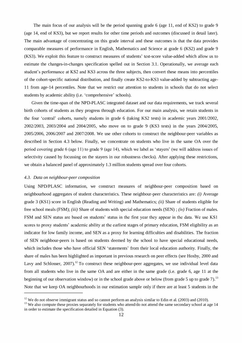
The main focus of our analysis will be the period spanning grade 6 (age 11, end of KS2) to grade 9

(age 14, end of KS3), but we report results for other time periods and outcomes (discussed in detail later).

The main advantage of concentrating on this grade interval and these outcomes is that the data provides

comparable measures of performance in English, Mathematics and Science at grade 6 (KS2) and grade 9

(KS3). We exploit this feature to construct measures of students‟ test-score value-added which allow us to

estimate the changes-in-changes specification spelled out in Section 3.1. Operationally, we average each

student‟s performance at KS2 and KS3 across the three subjects, then convert these means into percentiles

of the cohort-specific national distribution, and finally create KS2-to-KS3 value-added by subtracting age-

11 from age-14 percentiles. Note that we restrict our attention to students in schools that do not select

students by academic ability (i.e. „comprehensive‟ schools).

Given the time-span of the NPD-PLASC integrated dataset and our data requirements, we track several

birth cohorts of students as they progress through education. For our main analysis, we retain students in

the four „central‟ cohorts, namely students in grade 6 (taking KS2 tests) in academic years 2001/2002,

2002/2003, 2003/2004 and 2004/2005, who move on to grade 9 (KS3 tests) in the years 2004/2005,

2005/2006, 2006/2007 and 2007/2008. We use other cohorts to construct the neighbour-peer variables as

described in Section 4.3 below. Finally, we concentrate on students who live in the same OA over the

period covering grade 6 (age 11) to grade 9 (age 14), which we label as „stayers‟ (we will address issues of

selectivity caused by focussing on the stayers in our robustness checks). After applying these restrictions,

we obtain a balanced panel of approximately 1.3 million students spread over four cohorts.

4.3. Data on neighbour-peer composition

Using NPD/PLASC information, we construct measures of neighbour-peer composition based on

neighbourhood aggregates of student characteristics. These neighbour-peer characteristics are: (i) Average

grade 3 (KS1) score in English (Reading and Writing) and Mathematics; (ii) Share of students eligible for

free school meals (FSM); (iii) Share of students with special education needs (SEN) ; (iv) Fraction of males.

FSM and SEN status are based on students‟ status in the first year they appear in the data. We use KS1

scores to proxy students‟ academic ability at the earliest stages of primary education, FSM eligibility as an

indicator for low family income, and SEN as a proxy for learning difficulties and disabilities. The fraction

of SEN neighbour-peers is based on students deemed by the school to have special educational needs,

which includes those who have official SEN „statements‟ from their local education authority. Finally, the

share of males has been highlighted as important in previous research on peer effects (see Hoxby, 2000 and

Lavy and Schlosser, 2007).12 To construct these neighbour-peer aggregates, we use individual level data

from all students who live in the same OA and are either in the same grade (i.e. grade 6, age 11 at the

beginning of our observation window) or in the school grade above or below (from grade 5 up to grade 7).13

Note that we keep OA neighbourhoods in our estimation sample only if there are at least 5 students in the

12 We do not observe immigrant status and so cannot perform an analysis similar to Edin et al. (2003) and (2010).

13 We also compute these proxies separately for students who attend/do not attend the same secondary school at age 14

in order to estimate the specification detailed in Equation (3).

13

OA in these grade/age categories. Note too that we keep a balanced panel of students with non-missing

information in all years, so that neighbourhood quality changes are driven by the same students moving in

and out of the local area, and not by students joining in and dropping out of our sample. Given the quality

of our data, this restriction amounts to excluding approximately 2% of the initial sample.

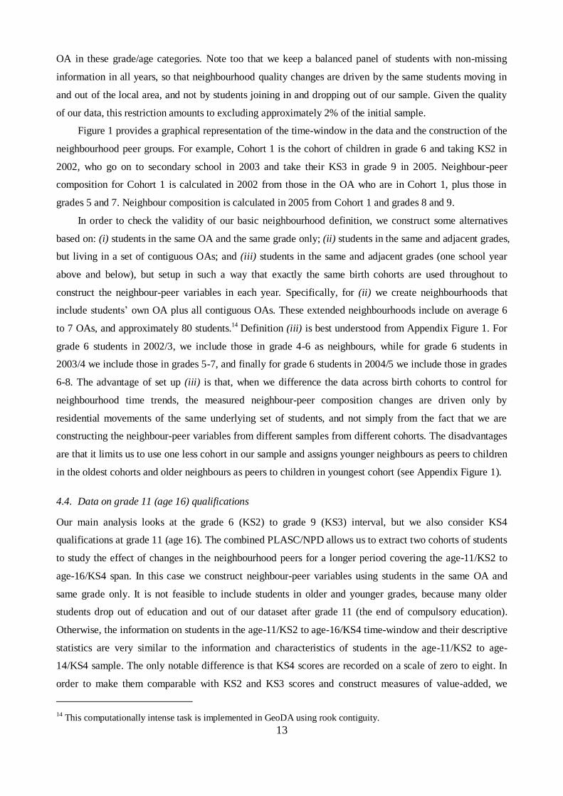
Figure 1 provides a graphical representation of the time-window in the data and the construction of the

neighbourhood peer groups. For example, Cohort 1 is the cohort of children in grade 6 and taking KS2 in

2002, who go on to secondary school in 2003 and take their KS3 in grade 9 in 2005. Neighbour-peer

composition for Cohort 1 is calculated in 2002 from those in the OA who are in Cohort 1, plus those in

grades 5 and 7. Neighbour composition is calculated in 2005 from Cohort 1 and grades 8 and 9.

In order to check the validity of our basic neighbourhood definition, we construct some alternatives

based on: (i) students in the same OA and the same grade only; (ii) students in the same and adjacent grades,

but living in a set of contiguous OAs; and (iii) students in the same and adjacent grades (one school year

above and below), but setup in such a way that exactly the same birth cohorts are used throughout to

construct the neighbour-peer variables in each year. Specifically, for (ii) we create neighbourhoods that

include students‟ own OA plus all contiguous OAs. These extended neighbourhoods include on average 6

to 7 OAs, and approximately 80 students.14 Definition (iii) is best understood from Appendix Figure 1. For

grade 6 students in 2002/3, we include those in grade 4-6 as neighbours, while for grade 6 students in

2003/4 we include those in grades 5-7, and finally for grade 6 students in 2004/5 we include those in grades

6-8. The advantage of set up (iii) is that, when we difference the data across birth cohorts to control for

neighbourhood time trends, the measured neighbour-peer composition changes are driven only by

residential movements of the same underlying set of students, and not simply from the fact that we are

constructing the neighbour-peer variables from different samples from different cohorts. The disadvantages

are that it limits us to use one less cohort in our sample and assigns younger neighbours as peers to children

in the oldest cohorts and older neighbours as peers to children in youngest cohort (see Appendix Figure 1).

4.4. Data on grade 11 (age 16) qualifications

Our main analysis looks at the grade 6 (KS2) to grade 9 (KS3) interval, but we also consider KS4

qualifications at grade 11 (age 16). The combined PLASC/NPD allows us to extract two cohorts of students

to study the effect of changes in the neighbourhood peers for a longer period covering the age-11/KS2 to

age-16/KS4 span. In this case we construct neighbour-peer variables using students in the same OA and

same grade only. It is not feasible to include students in older and younger grades, because many older

students drop out of education and out of our dataset after grade 11 (the end of compulsory education).

Otherwise, the information on students in the age-11/KS2 to age-16/KS4 time-window and their descriptive

statistics are very similar to the information and characteristics of students in the age-11/KS2 to age-

14/KS4 sample. The only notable difference is that KS4 scores are recorded on a scale of zero to eight. In

order to make them comparable with KS2 and KS3 scores and construct measures of value-added, we

14 This computationally intense task is implemented in GeoDA using rook contiguity.

14

average students‟ performance across Mathematics, Science and English and convert this mean into

percentiles in the cohort-specific national distribution. This method has been previously used when

analysing these data (e.g. Gibbons and Silva, 2008).

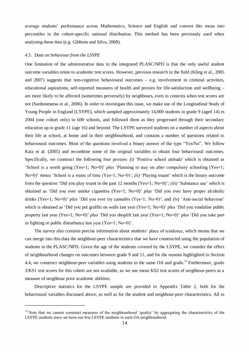
4.5. Data on behaviour from the LSYPE

One limitation of the administrative data in the integrated PLASC/NPD is that the only useful student

outcome variables relate to academic test scores. However, previous research in the field (Kling et al., 2005

and 2007) suggests that non-cognitive behavioural outcomes – e.g. involvement in criminal activities,

educational aspirations, self-reported measures of health and proxies for life-satisfaction and wellbeing –

are more likely to be affected (sometimes perversely) by neighbours, even in contexts when test scores are

not (Sanbonmatsu et al., 2006). In order to investigate this issue, we make use of the Longitudinal Study of

Young People in England (LSYPE), which sampled approximately 14,000 students in grade 9 (aged 14) in

2004 (one cohort only) in 600 schools, and followed them as they progressed through their secondary

education up to grade 11 (age 16) and beyond. The LSYPE surveyed students on a number of aspects about

their life at school, at home and in their neighbourhood, and contains a number of questions related to

behavioural outcomes. Most of the questions involved a binary answer of the type “Yes/No”. We follow

Katz et al. (2005) and recombine some of the original variables to obtain four behavioural outcomes.

Specifically, we construct the following four proxies: (i) „Positive school attitude' which is obtained as

„School is a worth going (Yes=1; No=0)‟ plus „Planning to stay on after compulsory schooling (Yes=1;

No=0)‟ minus „School is a waste of time (Yes=1; No=0)‟; (ii) „Playing truant‟ which is the binary outcome

from the question „Did you play truant in the past 12 months (Yes=1; No=0)‟; (iii) „Substance use‟ which is

obtained as „Did you ever smoke cigarettes (Yes=1; No=0)‟ plus „Did you ever have proper alcoholic

drinks (Yes=1; No=0)‟ plus „Did you ever try cannabis (Yes=1; No=0)‟; and (iv) „Anti-social behaviour‟

which is obtained as „Did you put graffiti on walls last year (Yes=1; No=0)‟ plus „Did you vandalise public

property last year (Yes=1; No=0)‟ plus „Did you shoplift last year (Yes=1; No=0)‟ plus „Did you take part

in fighting or public disturbance last year (Yes=1; No=0)‟.

The survey also contains precise information about students‟ place of residence, which means that we

can merge into this data the neighbour-peer characteristics that we have constructed using the population of

students in the PLASC/NPD. Given the age of the students covered by the LSYPE, we consider the effect

of neighbourhood changes on outcomes between grade 9 and 11, and for the reasons highlighted in Section

4.4, we construct neighbour-peer variables using students in the same OA and grade.15 Furthermore, grade

3/KS1 test scores for this cohort are not available, so we use mean KS2 test scores of neighbour-peers as a

measure of neighbour prior academic abilities.

Descriptive statistics for the LSYPE sample are provided in Appendix Table 2, both for the

behavioural variables discussed above, as well as for the student and neighbour-peer characteristics. All in

15 Note that we cannot construct measures of the neighbourhood „quality‟ by aggregating the characteristics of the

LSYPE students since we have too few LSYPE students in each OA neighbourhood.

15

all, these suggest that despite the fact that this sample is much smaller than our previous data, it is still

representative of the national population and displays enough variation in the variables of interest.

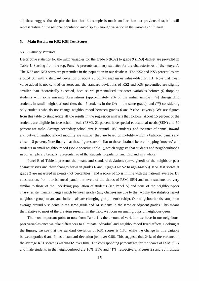
5. Main Results on KS2-KS3 Test Scores

5.1. Summary statistics

Descriptive statistics for the main variables for the grade 6 (KS2) to grade 9 (KS3) dataset are provided in

Table 1. Starting from the top, Panel A presents summary statistics for the characteristics of the „stayers‟.

The KS2 and KS3 sores are percentiles in the population in our database. The KS2 and KS3 percentiles are

around 50, with a standard deviation of about 25 points, and mean value-added on 1.1. Note that mean

value-added is not centred on zero, and the standard deviations of KS2 and KS3 percentiles are slightly

smaller than theoretically expected, because we percentalised test-score variables before: (i) dropping

students with some missing observations (approximately 2% of the initial sample); (ii) disregarding

students in small neighbourhood (less than 5 students in the OA in the same grade), and (iii) considering

only students who do not change neighbourhood between grades 6 and 9 (the „stayers‟). We use figures

from this table to standardize all the results in the regression analysis that follows. About 15 percent of the

students are eligible for free school meals (FSM), 21 percent have special educational needs (SEN) and 50

percent are male. Average secondary school size is around 1080 students, and the rates of annual inward

and outward neighbourhood mobility are similar (they are based on mobility within a balanced panel) and

close to 8 percent. Note finally that these figures are similar to those obtained before dropping „movers‟ and

students in small neighbourhood (see Appendix Table 1), which suggests that students and neighbourhoods

in our sample are broadly representative of the students‟ population and England as a whole.

Panel B of Table 1 presents the means and standard deviations (unweighted) of the neighbour-peer

characteristics and their changes between grades 6 and 9 (age-11/KS2 to age-14/KS3). KS1 test scores at

grade 2 are measured in points (not percentiles), and a score of 15 is in line with the national average. By

construction, from our balanced panel, the levels of the shares of FSM, SEN and male students are very

similar to those of the underlying population of students (see Panel A) and none of the neighbour-peer

characteristic means changes much between grades (any changes are due to the fact that the statistics report

neighbour-group means and individuals are changing group membership). Our neighbourhoods sample on

average around 5 students in the same grade and 14 students in the same or adjacent grades. This means

that relative to most of the previous research in the field, we focus on small groups of neighbour-peers.

The most important point to note from Table 1 is the amount of variation we have in our neighbour-

peer variables once we take differences to eliminate individual and neighbourhood fixed effects. Looking at

the figures, we see that the standard deviation of KS1 scores is 1.76, while the change in this variable

between grades 6 and 9 has a standard deviation just over 0.86. This suggests that 24% of the variance in

the average KS1 scores is within-OA over time. The corresponding percentages for the shares of FSM, SEN

and male students in the neighbourhood are 16%, 31% and 41%, respectively. Figures 2a and 2b illustrate

16

this point further by plotting the distributions of the neighbourhood mean variables: (i) levels (top left

panels), (ii) between-grade differences (top right panels), (iii) between-grade differences, after controlling

for primary-by-secondary-by-cohort school effects (bottom left panels); and (iv) between-grade, between-

cohort differences netting out OA trends (bottom right panels). All these figures suggest that there is

considerable variation over time in neighbour-peer characteristics, from which we can estimate our

coefficients of interest, and that controlling for school-by-cohort or OA trends does not lead to a drastic

reduction in this variation.

5.2. Neighbours’ characteristics and students’ test score: cross sectional and causal estimates

Table 2 presents our main regression results on the association between neighbour-peer characteristics and

students‟ test scores for the residential „stayers‟ sample. The table reports standardised regression

coefficients, with standard errors in parentheses (clustered at the OA level). As discussed in Section 4.3,

neighbour-peers are defined as students in the same OA and in the same or adjacent school grades, and we

report the effect of: average grade 3 (KS1) point scores (Panel A); share of FSM students (Panel B); share

of students with SEN status (Panel C); and share of male students (Panel D). Each coefficient is obtained

from a separate regression, i.e. we enter one neighbour-peer characteristic at a time. Clearly, some of these

neighbour-peer characteristics are very highly correlated with one another, but our aim is to look for effects

from any one of them – interpreted as an index of neighbour-peer quality – rather than the effect of each

characteristic conditional on the other. Columns (1)-(4) present results from regressions that do not include

control variables other than cohort dummies and/or other fixed effects as specified at the bottom of the table.

Columns (5)-(8) add in control variables for students‟ own characteristics as described later in this section.

The note to the table provides more details.

Column (1) shows the cross-sectional association between neighbour-peer characteristics and students‟

own KS3 test scores. All four characteristics are strongly and significantly associated with students‟ KS3

scores. A one standard deviation increase in KS1 scores is associated with a 0.3 standard deviation increase

in KS3, while a one standard deviation increase in FSM or SEN students is linked to a 0.2-0.3 standard

deviation reduction in KS3. The fraction of males has a small positive relation with KS3 scores.

However, these cross-sectional estimates are almost certainly biased by residential sorting and

unobserved individual, school and neighbourhood factors (as discussed in Sections 1 and 3). In order to

tackle this problem, we first eliminate student and neighbourhood unobserved fixed effects by estimating

within-student, between-grade differenced specifications as set out in Equations (2.1)-(2.2). The

corresponding results in Column (2) show that the associations between changes in neighbour-peer

characteristics and KS2-to-KS3 value-added are driven down almost to zero and only significant in two out

of the four panels. The coefficients are up to 100 times smaller than in Column (1). A one standard

deviation change in neighbour KS1 scores and in the FSM proportion over the three-year interval is linked

to a mere 0.3-0.5% of a standard deviation change in students‟ test-score progression. Neighbours‟ SEN

17

and male proportions are no longer significantly associated with students‟ KS2-to-KS3 value-added, and

their estimated effects are close to zero.

As discussed in Section 3, it is still possible that estimates from these within-student between-grade

differenced models are biased by unobserved school specific factors and neighbourhood trends. In order to

control for school specific factors, Columns (3) adds primary-by-secondary-by-cohort fixed effects that

absorb any cohort-specific shock to changes in school quality when moving from the primary to the

secondary phase. Results from these specifications show that none of the neighbour-peer characteristics are

now significantly related to students‟ KS2-to-KS3 value-added. The loss in significance is not due to a

dramatic increase in the standard errors, but to the magnitude of the coefficients shrinking towards zero.

This further backs the intuition gathered from Figures 2a and 2b that in principle there is sufficient

variation to identify significant associations between neighbourhood composition and students‟

achievements. In order to control for neighbourhood (OA) specific time trends, Column (4) further adds

OA fixed effects in the value-added specification, but the results are nearly identical to those in Column (3).

16 As shown in Appendix Table 3, accounting for OA trends only, without school-by-cohort effects, yields

virtually identical results.

Columns (5)-(8) repeat the analysis of columns (1)-(4), but add other characteristics as control

variables in the regression (namely, students‟ own KS1 scores, FSM and SEN status and gender, plus

school size, school type dummies and average rates of inward and outward mobility in the neighbourhood).

Comparing Columns (1) and (4) suggests that the cross sectional associations in Column (1) are severely

biased by sorting and unobserved student characteristics since adding in the control variables reduces the

coefficients substantially (by a factor of three). In contrast, it is important to notice that, once we eliminate

student and neighbourhood fixed effects in Columns (2) and (6), adding in the control set does not

significantly affect our results. The only case where there is a notable change is in the effect of neighbour-

peer SEN, which becomes statistically significant (at the 5% level), even though the point estimate is

virtually unchanged. The similarity of the results in Columns (2)-(4) with those in Columns (6)-(8) is

reassuring since it suggests that changes in neighbour-peer composition are not strongly linked to students‟

background characteristics. This finding lends initial support to our identification strategy which relies on

changes in the treatment variables to be „as good as random‟ once we partial out student and neighbourhood

fixed effects. The next section presents more formal evidence on this point.

Once concern might be that the attenuation in the estimates once we difference the data within-student

between-grades is caused by inflation in the noise to signal ratio because of noise in our neighbour-peer

variables. Although our proxies are constructed from administrative data on the population of state school

children, they may still be noisy measures of the „true‟ neighbour attributes that matter for students‟

achievements (which we cannot observe), and this noise could be exacerbated by differencing the data (in

16 Note that school-by-cohort effects and neighbourhood specific time trends do not capture the same things because

there is not a one-to-one mapping between neighbourhood of residence and school attended. Note also that including

primary-by-secondary-by-cohort effects and OA trends proved computationally not feasible, so we replaced the

former with secondary-by-cohort effects.

18

particular since there is a high degree of serial correlation in the neighbour-peer characteristics within

neighbourhoods). To systematically assess this issue, we performed two robustness checks. First, we used

teachers‟ assessment of students‟ performance during KS1 to construct instruments for neighbour-peer KS1

test scores on the grounds that the only common components of KS1 test scores and teacher assessments

should be related to „true‟ underlying neighbours‟ abilities. Instrumental variable (2SLS) regressions

confirmed that the effect of changes in KS1 test scores of neighbour-peers is not a strong and highly

significant predictor of students‟ KS2-to-KS3 value-added. Next, in our second robustness check, we

estimated a linear predictor of students‟ KS2 achievement by regressing students‟ own KS2 achievements

on own KS1 test scores, FSM eligibility, SEN status and gender. The predictions from these regressions

were then aggregated across neighbour-peers to create new measures of predicted neighbour-peer KS2 at

grade 6 and grade 9. This new composite indicator should be less affected by measurement error in relation

to the „true‟ neighbourhood quality that matters for students‟ achievements since it is based on the best

linear combination of the individual characteristics that predicts KS2 test scores. Using this measure as a

proxy for neighbour-peer „quality‟ produces similar results to those in Table 2, with no evidence of any

sizeable, significant effect from neighbours on students‟ achievement. It is also worth noting that the

reduction in coefficients from Column (2) to (3) and from Column (6) to (7) is not simply due the inclusion

of a large number of fixed effects (around 190,000 primary-by-secondary-by-cohort groups). As shown by

the estimates in Appendix Table 3, including only secondary school fixed effects (around 3200 groups) or

secondary-by-cohort effects (approximately 12,000 groups) similarly drives our estimates to zero.17

In summary, our baseline results indicate that the effects of neighbour-peers on student achievement

are statistically insignificant and/or negligibly small. In the following sections we assess our identifying

assumptions and present several extensions and robustness tests. Since controlling for unobserved

neighbourhood trends does not affect our main estimates, once we have taken into account school-by-

cohort effects, the analysis that follows only considers only the basic grade-differenced value-added

specifications (like Columns (2) and (6)) and specifications that further control for school cohort-specific

effects (like Column (3) and (7)).

5.3. Assessing our identification strategy

The validity of our empirical method rests on the assumption that changes in neighbour-peer composition

between grades are not related to the unobserved characteristics of students who stay in the neighbourhood

over the grade interval, nor to other unobservable attributes of the neighbourhoods. We have shown already

that the results of the between-grade within-individual value-added specifications are insensitive to whether

or not we include additional individual, school and neighbourhood mobility control variables, which

17 Note that as a further robustness check we replaced school fixed effects with school-level characteristics. For

example, we replaced primary-by-secondary-by-cohort effects with actual cohort-specific changes in school-level

characteristics on transition from primary to secondary school. These included student-to-teacher ratios, fraction of

students of White ethnic origin, fractions of students eligible for FSM and with SEN, number of full-time equivalent

(FTE) qualified teachers, and numbers of support teachers for ethnic minorities and SEN students. These

specifications confirmed that neighbourhood composition is not strongly associated with students‟ value-added.

19

supports the validity of the identifying assumptions. In this section, we tackle this issue more systematically

by providing evidence that our treatments are balanced with respect to student and neighbourhood

characteristics.

The neighbourhood characteristics we consider are drawn from the GB 2001 population census at OA

level. Specifically, we consider proportions of: (i) households living in socially rented accommodation; (ii)

owner-occupiers; (iii) adults in employment; (iv) adults with no qualifications; (v) lone parents. Additional

characteristics are generated by collapsing some salient student characteristics from our NPD data to OA

level, based on OA of residence at grade 6 (age 11), namely: KS1 test scores, FSM and SEN status and

gender, as well as the mean and the standard deviation of students‟ KS2 test scores. We carry out simple

cross-sectional OA level regressions of these neighbourhood characteristics on the OA-specific changes in

neighbour-peer characteristics that we used in the regressions in Table 2 (i.e. grade 6-to-9 changes in

neighbour-peer KS1 test scores, and FSM, SEN and male proportions).

Standardised coefficients and standard errors from these regressions are reported in Table 3. The top

panel shows the association between OA-mean student characteristics and the change in neighbour-peer

composition between grades 6 and 9. These regressions have no control variables other than the proportion

of students in the neighbourhood from each cohort in our data and the proportions of students represented

in different school types.18 The only significant and meaningful associations that we detect are related to the

changes in neighbour-peer FSM. The sign of these estimates suggests that neighbourhoods with low KS1,

high FSM and high SEN experience increases in fraction of neighbours who are FSM-registered, which

would imply upward biases in the estimates in Table 2, Columns (2)-(4). However, these associations are

very small in magnitude. Moreover, it should be noted that we have only imperfect controls for cohort and

school effects in these balancing tests, and these factors are more effectively controlled for in the

specifications in Table 2 which include school-by-cohort effects and neighbourhood trends.

In the bottom panel of Table 3 we regress OA-level KS2 statistics and Census variables on the

neighbour-peer change variables. These regressions further include OA-level averages of the controls added

in the specifications of Columns (4) to (8) of Table 2. The intuition for this approach is based on the idea of

using Census characteristics and OA KS2 statistics as proxies for additional unobservable factors in the

regressions of Columns (4)-(8), and testing for their correlation with the changes in neighbour-peer

characteristics to see if these unobservable OA factors drive neighbourhood composition. The results

present a reassuring picture: nearly all the estimated coefficients are very small and insignificant.

Overall, the balancing tests in Table 3 provided no evidence of strong associations between neighbour-

peer changes and other neighbourhood characteristics, and provide no evidence that the near-zero

neighbour-peer effect estimates in Table 2 are downward biased by student or neighbourhood

unobservables.

18 School „types‟ include: Community, Voluntary Aided, Voluntary Controlled, Foundation, City Technology College

and Academy. The cohort and school type proportions stand in for the cohort-by-school effects in our main student

level regressions, which we are unable to include in the aggregated OA-level regressions.

20

5.4. Peers at school or peers in the neighbourhood?

In the analysis conducted so far, we have not distinguished between neighbour-peers who attend the same

secondary school, and those who do not. However, this distinction could be important for a number of

reasons. First, children who are at school for a large part of their day may simply not interact with

neighbours, unless they know each other from school already. In this case, neighbour-peers who attend a

different school may exert little or no influence on students‟ outcomes. Secondly, distinguishing between

school and neighbourhood peers is more generally useful for uncovering a „pure‟ neighbourhood level peer

effect, net of interactions that happen at school (i.e. school peer effects) and other school factors that have

not otherwise been effectively controlled for in our regressions.

Table 4 presents evidence on this issue by tabulating results obtained from the specifications detailed

in Equation (3), and including different levels of fixed effects as we move from Column (1) to Column (4).

The sample used to estimate these specifications is slightly smaller than the one used to obtain the results

presented in Table 2 since we drop neighbourhoods in which all students attend the same school, or all

students attend different schools. Results in Column (1), Panel A show that neighbour-peer KS1 has an

impact on a student‟s achievement only if these neighbours also attend that student‟s secondary school.

However, in line with our previous findings, this association vanishes as soon as we include secondary-by-

cohort or primary-by-secondary-by-cohort effects. Next, results in Panel B, Column (1) show that FSM

status of neighbour-peers matters irrespective of school attended, with a standardised coefficient of negative

0.003 (s.e. 0.001). Again, as soon as we include school-by-cohort effects to control for the school-related

residential sorting during the transition between primary and secondary school, the estimated effects shrink

and become insignificant. Similarly, we find no evidence of neighbour-peer effects when looking at

neighbours‟ SEN-status and gender, irrespective of the school attended.

All in all, the evidence gathered in this section rejects the hypothesis that neighbourhood peers matter

differentially depending on whether they attend the same school or not. More importantly, this evidence

confirms our conclusion that neighbourhood peer effects – in particular „pure‟ neighbourhood peer effects,

not confounded by interactions at school – do not matter for students‟ test score progression.

5.5. Robustness checks: intention-to-treat estimates, alternative definitions of neighbourhoods and peers,

and other estimation samples

An important issue that we already flagged in both Sections 3 and 4 is that, by focussing on the sample of

students who stay in the same neighbourhood between grades 6 and 9, we might induce some bias due to

endogenous sample-selection. To circumvent this problem, we estimate the grade-differenced specification

in Equation (2.1) using both „stayers‟ and students who move neighbourhood between grades 6 and 9. At

grade 9, we assign to these „movers‟ the grade-9 characteristics of the neighbourhood in which they lived at

grade 6. Stated differently, we assign them to the changes in the neighbourhood „quality‟ that they would

have experienced had they not moved. Estimates obtained following this approach are more properly

interpreted as intention-to-treat effects. Table 5 presents the results from specifications as in Equation (2.1)

21

both without (Column (1)) and with (Column (2)) primary-by-secondary-by-cohort effects (both columns

include our standard control variables). The new results are almost identical to those reported in Table 2 for

the stayers only, allaying sample-selection concerns.

As discussed in Section 3.3, there are ambiguities about the correct neighbour-peer group definition.

Given we cannot know a priori the correct grouping, we experiment in Table 5 with different group

definitions as discussed in Section in 4.3. Columns (3) and (4) consider neighbour-peers in the same OA

and grade. Column (5) and (6) base neighbour-peer variables on the same group of birth cohorts in each

year, such that our neighbour-peer variables do not change due to sampling of different cohorts, even when

there is no real underlying demographic change. Finally, Columns (7) and (8) change the neighbourhood

definition to include, on average, 6-7 adjacent OAs (on average 80 students). In general, these re-definitions

make no substantive difference to the results. In some cases, previously insignificant coefficients become

more precise, although all the effects remain very small in magnitude, and most are insignificant once we

include school-by-cohort effects. It is worth noting that using aggregates computed over larger residential

areas in Column (7) increases the precision and the size of our estimates. However, including school-by-

cohort effects as in Column (8) brings our estimates close to zero and insignificant (with the exception of

the changes in the share of males). This pattern might be explained by the fact that changes in larger

neighbourhood aggregates are more likely to be „contaminated‟ by omitted time-varying neighbourhood

factors – such as changes to neighbourhood infrastructure or household mobility dictated by school quality

and access – than for smaller geographical units. This lends support to our claim made earlier that, since our

identification approach relies on fixed effects to control for neighbourhood unobservables, a small scale is

desirable in order to minimise the risk of endogeneity of changes in neighbourhood quality.

Finally, we also tried alternative neighbour-peer variables based on the adult population in the

neighbourhood (rather than students of similar ages). This type of information is not readily available from

the education datasets used so far, but was collected using time-varying information gathered by the

Department for Work and Pension (DWP) on people claiming unemployment benefits and income support.

More specifically, we were able to match to the various cohorts of students going through secondary

education some information on: (i) the number of working-age people claiming the „Job Seeker Allowance‟

(JSA, i.e. unemployment benefits); (ii) the number of people aged 16-25 claiming JSA; and (iii) the number

of lone parents on income support (a proxy for very low income usually among young un-married mothers).

Evidence from this analysis (not tabulated, but available from the authors) gives no support to the idea that

adults‟ characteristics affect students‟ test-score progression. Once we control for school-by-cohort effects

and/or neighbourhood unobserved trends, our estimates become very small and insignificant. This suggests

that interactions with neighbouring adults and/or role models, do not significantly affect students' school

test score outcomes.

22

5.6. Heterogeneity and non-linearity in the estimated neighbourhood effects

Our results so far suggest that changes in neighbour-peer composition do not influence students‟ test score

gains. This headline results might mask a significant degree of heterogeneity along a number of dimensions,

although our empirical investigation of this issue revealed little evidence of this heterogeneity (full results

are in Appendix Tables 4 and 5). In particular, we looked at differences according to whether that student:

(i) has KS1 test scores above/below the sample median; (ii) is eligible for FSM; (iii) has SEN status; (iv) is

male or female. Out of the thirty-two estimates only four were significant at conventional levels: a larger

fraction of SEN students negatively affects students with high KS1 achievements; a larger fraction of FSM

students lowers non-SEN and female students‟ test-scores; a larger fraction of boys improves other boys‟

achievements. However, all of these effects were only significant at the 5% level and represented very

small effects. Moreover, they did not present a consistent picture with weaker/stronger students from

poorer/wealthier family backgrounds being affected differently. All in all, these results lend support to our

previous conclusions.

Looking at differences across neighbour-peer characteristics gives a similar picture. We compared

neighbourhoods with: (i) above/below median student numbers; (ii) above/below median population

density; (iii) above/below median housing over-crowding19; and (iv) a percentage of social housing tenants

above/below 75%. Only two out of these thirty-two coefficients were significant at conventional levels: the

fraction of neighbours with FSM and SEN status has a significantly adverse effect on the value-added of

students living high density neighbourhoods, but again, the effect sizes are small. To investigate these

findings further, we also looked for potential heterogeneity in our estimates by separately considering the

ten biggest cities versus the rest of England, and London versus the rest of England. However, we failed to

find any significant pattern. Once again, our main conclusions were confirmed.

We have also investigated potential non-linearities and thresholds in neighbourhood peer effects.20 We

used specifications that: (i) included quadratic and cubic powers of the four neighbourhood composition

variables (e.g. the change in the squared fraction of FSM students); (ii) included quadratic and cubic powers

of the changes in our proxies (e.g. the change in the fraction of FSM students squared); (iii) allowed

positive and negative neighbourhood changes to cause different effects (e.g. an increase vs. a decrease in

the average KS1 of peers in the neighbourhood); (iv) allowed for large-negative, negative, positive and

large-positive changes to have different effects; (v) allowed for distinct effects from the very highest and

the very lowest ability neighbours (pupils in the top and bottom 5% of KS1 distribution; Lavy et al., 2011

provide some related evidence for peers in English secondary schools). However, we still failed to find any

significant effect. All in all, our main conclusions remain unaffected: neighbours‟ ability and characteristics

do not affect students‟ test-score progression between grades 6 and 9.

19 This proxy is based on the Census definition which identifies households in over-crowded housing if more than one

person occupies a room (excluding bathrooms). 20

These findings are not tabulated for space reasons, but are available upon requests.

23

6. Results on achievement at other ages and on behavioural outcomes

6.1. Students’ achievements at age 16 and at primary school

The analysis in Section 5 concentrated on the grade 6 to grade 9 changes. In this section, we investigate

other outcomes and grade intervals. To begin with, we consider students‟ attainments at grade 11 (KS4) and

analyse whether students‟ value-added between grade 6 (KS2) and grade 11 (KS4), and between grade 9

(KS3) and grade 11 (KS4) is affected by the corresponding changes in neighbour-peer characteristics. The

data used to estimate these models is discussed in Section 4.3. The most important issues to recall are that

because of data limitations: (i) we can only construct aggregates of neighbourhood quality using students in

the same OA and grade; and (ii) we can only use two cohorts, and as a consequence we replace school-by-

cohort effects with secondary school fixed effects in our specifications. A selection of our results is

presented in Table 6. Columns (1) and (2) concentrate on the value-added between KS2 and KS4. For all

four neighbour-peer characteristics, results show no significant effect on progression through secondary

education, irrespective of whether or not we control for school fixed effects. Next, in Column (3) and (4),

we look at KS3 to KS4 changes, but still fail to find any significant association. As an additional test and to

allow for time lags in the process by which neighbour changes influence students, we investigated whether

grades 9-to-11 (KS3-to-KS4) value-added is affected by changes in the neighbourhood composition

between grades 6 and 9 (i.e. over the KS2 to KS3 phase), or between grades 8 and 10 (i.e. one-year lag with

respect to the Key Stage tests). Again, we failed to document significant neighbourhood effects. Finally, we

also looked at students‟ value-added in primary school (results not tabulated), replicating the analysis in

Table 2 for the grade 2 to grade 6 (KS1 to KS2) phase. Again, we found no evidence of significant

neighbour-peer effects on students‟ test-score value-added.

6.2. Neighbourhood characteristics and behavioural outcomes: evidence from the LSYPE

As discussed in Section 4.5, the major limitations of the integrated PLASC/NPD data used so far is that the

only useful student outcome variables relate to academic test scores. In order to consider potentially more

interesting effects of neighbour-peer composition on behaviour, we use information collected in the

Longitudinal Survey of Young People in England (LSYPE), linked to the NPD-based neighbour-peer

variables used throughout the analysis so far. Given the time-window considered by the LSYPE, we can

only consider the effect of neighbourhood changes on outcomes between grade 9 and grade 11. Moreover,

age-7 test scores for this cohort are not available, so we aggregate the levels of the KS2 test scores of

neighbouring students to proxy for prior academic ability. We report the results from our investigation in

Table 7. Since previous evidence in the literature has shown a significant degree of heterogeneity along the

gender dimension, we report estimates from separate regressions for boys and girls. All models include the

standard set of controls and secondary school fixed effects. The construction of the behavioural outcome

variables is documented in Section 4.5.

Columns (1) and (2) tabulate the relation between neighbourhood changes and the composite variable

„Positive school attitude' for boys and girls, respectively. Starting from the top, we see that an improvement

24

in grade 7 (KS2) achievements of neighbour-peers positively affects students‟ attitudes towards education,

and that this effect is significant and sizeable for boys: a one standard deviation change in the treatment

corresponds to a 3.6% of a standard deviation change in the dependent variable. Symmetrically, we find

that a larger share in the fraction of neighbours with learning difficulties and poor achievements (as

captured by SEN status; see Panel C) negatively affects views about schooling, but this effect is only

significant and sizeable for girls. In this case, a one standard deviation increase in the treatment would

negatively affect female students‟ attitudes towards education by 6.4% of a standard deviation. On the other

hand, neither the fraction of students in the neighbourhood who are eligible for FSM nor the share of males

affects other students‟ views of education.

Next, in the four central columns of the table we investigate the relation between neighbour-peer

composition and students‟ absences from school („Playing Truant‟; Columns (3) and (4)) and students‟ use

of substances (this proxy includes smoking, drinking and using cannabis; see Columns (5) and (6)). None of

the associations presented in the table is significant at conventional levels, and often the signs of these

relations are the opposite of what one would expect. All in all, there does not seem to be any effect of

neighbourhood composition on these two outcomes.

Finally, in Columns (7) and (8) we concentrate on the variable „anti-social behaviour‟, which captures

whether students got involved in putting graffiti on walls, vandalising property, shoplifting, and whether

they took part in fighting or public disturbance. Our results show that, while neighbourhood composition in

terms of KS2 achievements, share of males and proportion of students with SEN status does not

significantly affect these behavioural outcomes, an interesting pattern emerges when looking at the

proportion of neighbours from poor family background (FSM; see Panel B). A one standard deviation

change in this treatment would significantly increase male students‟ involvement in anti-social behaviour

by 5% of a standard deviation, but this change would not affect young girls‟ behaviour.21

These differential effects for boys and girls are not surprising. Kling et al. (2005) and (2007) document

similarly heterogeneous effects for male and female youths „re-assigned‟ to better neighbourhoods by the

MTO experiment. More broadly, a growing body of research shows that boys and girls respond differently

to education-related interventions. Amongst others, Anderson (2008) finds that three well-known early

childhood interventions (namely, Abecedarian, Perry and the Early Training Project) had substantial short-

and long-term effects on girls, but no effect on boys, while Lavy et al. (2011) find that peer quality in

English secondary schools affects boys and girls differently. Similarly, recent studies show a consistent

pattern of stronger female response to financial incentives in education, with the evidence coming from a

variety of settings (see Angrist and Lavy, 2009; Angrist et al., 2009).

21 Note that we also studied whether the effects of neighbours‟ characteristics on boys‟ and girls‟ behavioural

outcomes differ according to peers‟ gender. Our evidence shows that male peers‟ FSM eligibility has a larger effect

than female peers‟ FSM status on male students‟ involvement in anti-social behaviour. Additionally, male peers‟ SEN

status is more strongly linked to girls‟ attitudes towards education than female peers‟ SEN condition. However, neither

of these differences was statistically significant.

25

In conclusion, and considering both the small number of students sampled by the LSYPE and the fact

that we can only look at outcomes between grade 9 and 11, the results in Table 7 provide some support for

the notion the neighbourhoods can affect teenagers‟ behaviour. However, all in all our evidence also

suggests that neighbour-peer effects are not a strong and pervasive determinant of students‟ cognitive and

non-cognitive outcomes.

7. Concluding Remarks

Our study has used various detailed administrative datasets on the population of students in England to

study the effect of the characteristics and prior achievements of peers in the neighbourhood on the

educational achievements and behavioural outcomes of secondary school students. In our main sample we

track over 1.3 million students across four cohorts that go through the first three years of their secondary

schooling. Our findings show that, although there is a substantial cross-sectional correlation between

students‟ test scores and the characteristics of their residential neighbourhoods, there is no evidence that

this association is causal. The „true‟ effect of changes in peers in the neighbourhood on students‟ test-score

gains between grades 6 (ages 11) and 9 (age 14) is nil.

In order to assess the robustness of this conclusion, we have extended our analysis in a number of

dimensions. First, we have distinguished between peers in the neighbourhood that attend the same school

and those who do not. Next, we have considered alternative definitions of neighbourhoods and different

ways of identifying peers in the place of residence, as well as investigated whether the relation between

neighbourhood composition and students‟ test scores is non-linear, or heterogeneous along the lines of

student background and neighbourhood characteristics. Finally, we have considered alternative time-

windows and looked at whether later (age-16, end of compulsory education) or earlier educational

achievements (during primary education) are affected by the characteristics of peers in the neighbourhood.

All in all, our evidence leads us to conclude that neighbourhood effects are a non-significant determinant of

students‟ test score attainments in schools.

On the other hand, we uncover some evidence that non-cognitive and behavioural outcomes – such as

attitude towards schools and anti-social behaviour – are affected by changes in neighbourhood composition,

and that these effects are heterogeneous along the gender dimension. While due to some data limitations

(stemming from sample size and timing) the results on behavioural outcomes are less conclusive, our

evidence is in line with previous findings in the literature.

Besides presenting new evidence on the effect of peers in the neighbourhood, our study makes a

number of important methodological contributions. First, we „drill down‟ to the effect of neighbourhood

changes that are caused by real movements of families in an out of small neighbourhoods. We can track

these changes through information on the detailed residential addresses of our census of students. This is

radically different from the approach used in the literature that looks at peer effects at schools, which

focuses on the year-on-year changes in school composition under the maintained assumption that students

only interact with peers within their grade (or class). Moreover, the English institutional setting where

26

secondary school attendance is not tightly linked to place of residence, allows us to distinguish between

neighbours who attend the same or a different school, and to test for potential interactions between school

and neighbourhood peer effects. Furthermore, by exploiting the detail and density of our data, we are able

to change our definitions of neighbourhoods and peers in the place of residence, and thus address the

inherent problem in the literature of pinning-down the correct definition of what constitutes „a

neighbourhood‟. This allows us to exclude the possibility that our findings are stemming from data-driven

incorrect levels of aggregation. Finally, exploiting the fact that we observe several cohorts of students

experiencing changes in the composition of their neighbourhoods at the same as they move through the

education system, we are able to partial out student and family background unobservables, neighbourhood

fixed effects and time trends as well as school-by-cohort unobserved shocks. We believe this is unique in

getting us close to pinning down an unbiased „neighbourhood effect‟ estimate stemming solely from social

interactions and role models in the place of residence as originally advocated by Moffit (2001).

27

8. References

Allen, R., S. Burgess and T. Key (2010): “Choosing Secondary School by Moving Home: School Quality and the Formation of Neighbourhood”, CMPO Working Paper, 10/238.

Aaronson, D. (1998): “Using Sibling Data to Estimate the Impact of Neighborhoods on Children's Educational Outcomes,” Journal of Human Resources, pp. 915-46.

Angrist, J.D., D. Lang and P. Oreopolous (2009): “Incentives and Services for College Achievement: Evidence from a Randomized Trial”, American Economic Journal: Applied Economics, 1.

Angrist, J.D. and V. Lavy: “The Effect of High-Stakes High School Achievement Awards: Evidence from a Randomized Trial,” American Economic Review, September 2009.

Akerlof, G. (1997): Social Distance and Social Decisions, Econometrica, 65(5), pp. 1005-1027.

Bayer, P., L. Ross, L. and G. Topa (2008): “Place of Work and Place of Residence: Informal Hiring Networks and Labour Market Outcomes,” Journal of Political Economy, 116(6): pp. 1150-1196.

Bernheim, B. (1994): “A Theory of Conformity,” The Journal of Political Economy, 102(5), pp. 841-877.

Black, S. (1999): “Do Better Schools Matter? Parental Valuation of Elementary Education,” The Quarterly Journal of Economics, 114(2), pp. 577-99.

Bolster A., Burgess S., Johnston R, K. Jones, C. Propper and R. Sarker (2007): “Neighbourhoods, households and income dynamics: a semi-parametric investigation of neighbourhood effects,” Journal of Economic Geography, 7(1), pp. 1-38

Card, D., and J. Rothstein (2007): “Racial Segregation and the Black-White Test Score Gap”, Journal of Public Economics, 91(11-12): 2158-2184.

Cheshire, P. and S. Sheppard (1995): “On the Price of Land and the Value of Amenities,” Economica, New Series, Vol. 62, No. 246 (May), pp. 247-267.

Cheshire, P., S. Gibbons, S. and I. Gordon (2008) “Policies for 'Mixed Communities': A Critical Evaluation,” SERC Policy Paper, 2.

Currie, J. (2006): The Invisible Safety Net, Princeton University Press, New Jersey, USA.

Cutler, D. and E. Glaeser (1997): “Are Ghettos Good Or Bad?,” The Quarterly Journal of Economics 112(3), pp. 827-72.

Durlauf, S. (1996): “A Theory of Persistent Income Inequality,” Journal of Economic Growth, pp. 75-93.

Edin, P., P. Fredriksson and O. Aslund (2003) “Ethnic Enclaves and the Economic Success of Immigrants – Evidence from a Natural Experiment”, Quarterly Journal of Economics, 118, pp. 329-357.

Edin, P., P. Fredriksson, H. Gronqvist and O. Aslund (2010) “Peers, Neighbourhoods and Immigrant Student Achievement – Evidence from a Placement Policy”, American Economic Journal: Applied Economics, accepted for publication.

Fehr, E. and A. Falk (2002): “Psychological Foundations of Incentives,” European Economic Review, 46(4-5), pp. 687-724.

Gibbons, S. (2002): “Neighbourhood Effects on Educational Achievement”, CEE Discussion Paper, CEEDP0018.

Gibbons, S., S. Machin and O. Silva (2008): “Choice, Competition and Student Achievement”, Journal of the European Economic Association, 6(4), pp. 912-947.

Gibbons, S., S. Machin and O. Silva (2009): "Valuing School Quality Using Boundary Discontinuities,” SERC Discussion Papers, 18.

Gibbons, S. and O. Silva (2008): “Urban Density and Student Attainment”, Journal of Urban Economics, 63(1), pp. 631-650.

28

Gibbons, S and S. Telhaj (2011): “Mobility and School Disruption,” Journal of Public Economics, forthcoming.

Gibbons, S and S. Telhaj (2008): “Peers and Achievement in England's Secondary Schools,” SERC Discussion Paper, 1.

Glaeser, E. and J. Scheinkman (2001): “Measuring Social Interactions,” in Social Dynamics, Durlauf, S. and P. Young (eds.), Boston, MA: MIT Press.

Glennerster, H. (1991): “Quasi-Markets for Education,” Economic Journal, 101, pp. 1268-76.

Gould, E., V. Lavy and D. Paserman (2004): “Immigrating to Opportunity: Estimating the Effect of School Quality using a Natural Experiment on Ethiopians in Israel,” Quarterly Journal of Economics, 119(2), pp. 489-526.

Gould, E., V. Lavy and D. Paserman (2011): “Sixty Years after the Magic Carpet Ride: The Long-Run Effect of the Early Childhood Environment on Social and Economic Outcomes,” Review of Economic Studies, 78(3), pp. 938-973.

Goux, D. and E. Maurin (2007): “Close Neighbours Matter: Neighbourhood Effects on Early Performance at School,” Economic Journal, 117(523), pp. 1193-215.

Granovetter, M. (1995): Getting a Job, second edition, Chicago, IL: University of Chicago Press.

Harding, D, L. Gennetian, C. Winship, L. Sanbonmatsu, J. Kling (2010): “Unpacking Neighborhood Influences on Education Outcomes: Setting the Stage for Future Research,” NBER Working Paper 16055.

Hanushek, E., J. Kain, J. Markman and S. Rivkin (2003): “Does Peer Ability Affect Student Achievement?”, Journal of Applied Econometrics, 18, pp. 527-544.

Hanushek, E., J. Kain and S. Rivkin (2004): “Disruption versus Tiebout improvement: the costs and benefits of switching schools”, Journal of Public Economics, 88, pp. 1721-1746

Hoxby, C. (2000): “Peer Effects in the Classroom: Learning from Gender and Race Variation,” NBER Working Paper 7867.

Jacob, B. (2004): “Public Housing, Housing Vouchers, and Student Achievement: Evidence from Public Housing Demolitions in Chicago,” The American Economic Review, 94(1), pp. 233-58.

Kain, J. and J. Quigley (1975): “The Demand for Individual Housing Attributes,” in: Housing Markets and Racial Discrimination: A Microeconomic Analysis, pages 231-255, National Bureau of Economic Research, Inc.

Kling, J., J. Liebman and L. Katz (2007): “Experimental Analysis of Neighborhood Effects,” Econometrica, pp. 83-119.

Kling, J., J. Ludwig and L. Katz (2005): “Neighborhood Effects on Crime for Female and Male Youth: Evidence From a Randomized Housing Voucher Experiment”, Quarterly Journal of Economics, 120, pp. 87-130.

Lavy, V., D. Paserman and A. Schlosser (2008): “Inside the Black Box of Ability Peer Effects: Evidence from Variation in Low Achievers in the Classroom,” NBER Working Paper 14415.

Lavy, V., and A. Schlosser (2007): “Mechanisms and Impacts of Gender Peer Effects at School,” NBER Working Paper 13292.

Lavy, V., O. Silva and F. Weinhardt (2011): “The Good, The Bad and The Average: Evidence on Ability Peer Effects in Schools”, Journal of Labor Economics, forthcoming.

Lupton, R. (2009): “Growing up in Social Housing in Britain”, Report: Joseph Rowntree Foundation, York.

Manski, C. (1993): “Identification of Endogenous Social Effects: The Reflection Problem,” Review of Economic Studies, 60, pp. 531-42.

Moffitt, R. (2001): “Policy interventions, Low-level Equilibria, and Social Interactions,” in Social Dynamics, Durlauf, S. and P. Young (eds.), Boston, MA: MIT Press.

29

Oreopolous, P. (2003): “The Long-Run Consequences of Living in a Poor Neighborhood,” Quarterly Journal of Economics, 118, pp. 1533-1575.

Rosenbaum, J. (1995): “Changing the Geography of Opportunity by Expanding Residential Choice: Lessons from the Gautreaux Program,” Housing Policy Debate, 6, pp. 231-69.

Sacerdote, B. (2001): “Peer Effects with Random Assignment: Results for Dartmouth Roommates,” Quarterly Journal of Economics, 116(2), 681-704.

Sampson, R., J. Morenoff and T. Gannon-Rowley (2002): “Assessing Neighbourhood Effects: Social Processes and New Directions in Research,” Annual Review of Sociology, 26, pp. 443-478.

Sanbonmatsu, L., J. Kling, G. Duncan and J. Brooks-Gunn (2006): “Neighborhoods and academic achievement: Results from the Moving to Opportunity Experiment,” Journal of Human Resources, 41(4), p. 649.

Weinhardt, F. (2010): “Moving into the Projects: Social Housing Neighbourhoods and School Performance in England”, SERC Discussion Paper, 44.

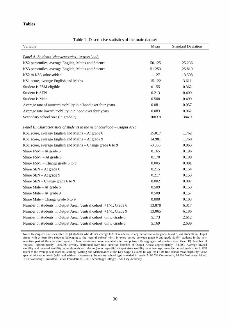
30

Tables

Table 1: Descriptive statistics of the main dataset

Variable Mean Standard Deviation

Panel A: Students’ characteristics, ‘stayers’ only

KS2 percentiles, average English, Maths and Science 50.125 25.236

KS3 percentiles, average English, Maths and Science 51.253 25.819

KS2 to KS3 value-added 1.127 13.598

KS1 score, average English and Maths 15.122 3.611

Student is FSM eligible 0.155 0.362

Student is SEN 0.213 0.409

Student is Male 0.508 0.499

Average rate of outward mobility in n‟hood over four years 0.081 0.057

Average rate inward mobility in n‟hood over four years 0.083 0.062

Secondary school size (in grade 7) 1083.9 384.9

Panel B: Characteristics of students in the neighbourhood – Output Area

KS1 score, average English and Maths – At grade 6 15.017 1.762

KS1 score, average English and Maths – At grade 9 14.981 1.760

KS1 score, average English and Maths – Change grade 6 to 9 -0.036 0.863

Share FSM – At grade 6 0.165 0.196

Share FSM – At grade 9 0.170 0.199

Share FSM – Change grade 6 to 9 0.005 0.081

Share SEN – At grade 6 0.215 0.154

Share SEN – At grade 9 0.217 0.153

Share SEN – Change grade 6 to 9 0.002 0.087

Share Male – At grade 6 0.509 0.153

Share Male – At grade 9 0.509 0.157

Share Male – Change grade 6 to 9 0.000 0.103

Number of students in Output Area, „central cohort‟ +1/-1, Grade 6 13.878 6.317

Number of students in Output Area, „central cohort‟ +1/-1, Grade 9 13.865 6.186

Number of students in Output Area, „central cohort‟ only, Grade 6 5.173 2.612

Number of students in Output Area, „central cohort‟ only, Grade 6 5.169 2.639

Note: Descriptive statistics refer to: (i) students who do not change OA of residence in any period between grade 6 and 9; (ii) students in Output

Areas with at least five students belonging to the „central cohort‟ +1/-1 in every period between grade 6 and grade 9; (iii) students in the non-

selective part of the education system. These restrictions were operated after computing OA aggregate information (see Panel B). Number of

„stayers‟: approximately 1,310,000 (evenly distributed over four cohorts). Number of Output Areas: approximately 134,000. Average inward

mobility and outward mobility in neighbourhood refer to (cohort-specific) Output Area mobility rates averaged over the period grade 6 to 9. KS1

refers to the average test score in Reading, Writing and Mathematics at the Key Stage 1 exams (at age 7); FSM: free school meal eligibility; SEN:

special education needs (with and without statements). Secondary school type attended in grade 7: 66.7% Community; 14.9% Voluntary Aided;

3.1% Voluntary Controlled; 14.5% Foundation; 0.3% Technology College; 0.5% City Academy.

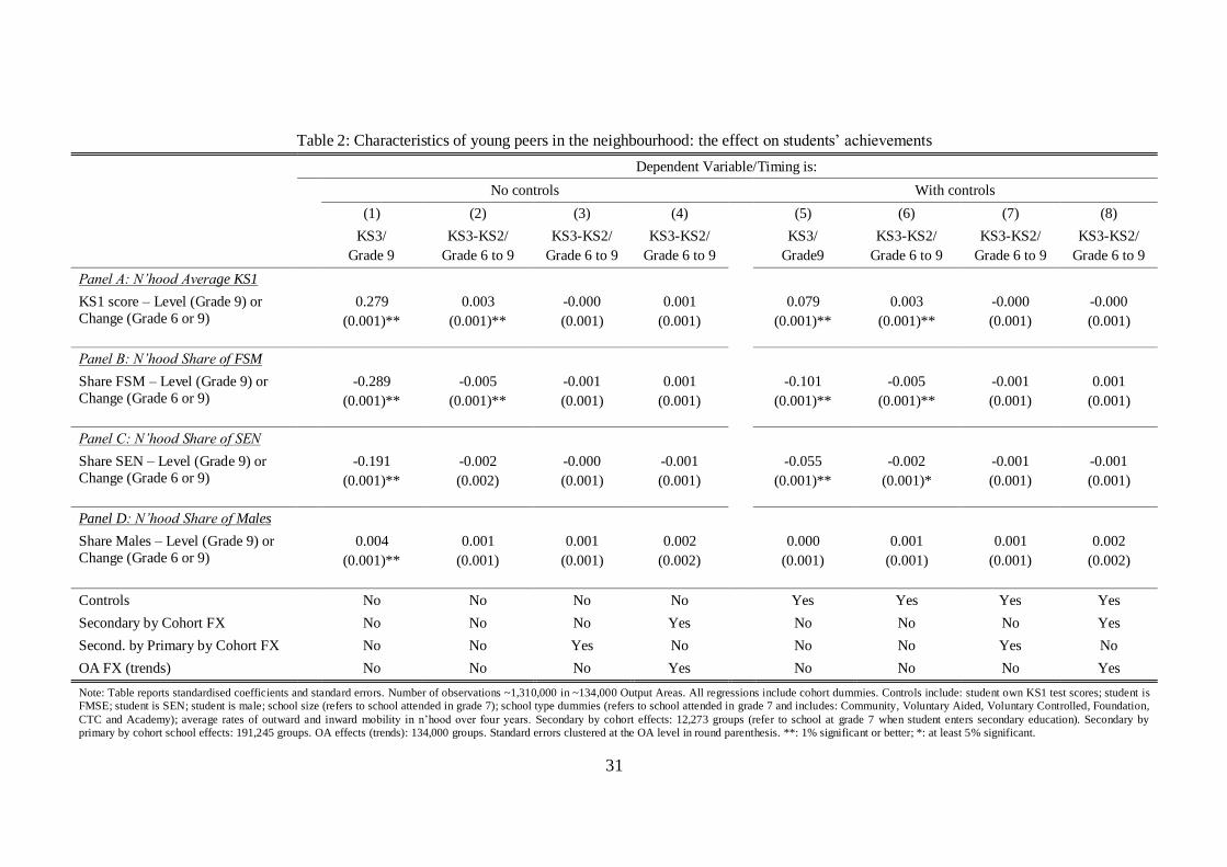
31

Table 2: Characteristics of young peers in the neighbourhood: the effect on students‟ achievements

Dependent Variable/Timing is:

No controls With controls

(1) (2) (3) (4) (5) (6) (7) (8)

KS3/

Grade 9

KS3-KS2/

Grade 6 to 9

KS3-KS2/

Grade 6 to 9

KS3-KS2/

Grade 6 to 9

KS3/

Grade9

KS3-KS2/

Grade 6 to 9

KS3-KS2/

Grade 6 to 9

KS3-KS2/

Grade 6 to 9

Panel A: N’hood Average KS1

KS1 score – Level (Grade 9) or

Change (Grade 6 or 9)

0.279

(0.001)**

0.003

(0.001)**

-0.000

(0.001)

0.001

(0.001)

0.079

(0.001)**

0.003

(0.001)**

-0.000

(0.001)

-0.000

(0.001)

Panel B: N’hood Share of FSM

Share FSM – Level (Grade 9) or

Change (Grade 6 or 9)

-0.289

(0.001)**

-0.005

(0.001)**

-0.001

(0.001)

0.001

(0.001)

-0.101

(0.001)**

-0.005

(0.001)**

-0.001

(0.001)

0.001

(0.001)

Panel C: N’hood Share of SEN

Share SEN – Level (Grade 9) or

Change (Grade 6 or 9)

-0.191

(0.001)**

-0.002

(0.002)

-0.000

(0.001)

-0.001

(0.001)

-0.055

(0.001)**

-0.002

(0.001)*

-0.001

(0.001)

-0.001

(0.001)

Panel D: N’hood Share of Males

Share Males – Level (Grade 9) or

Change (Grade 6 or 9)

0.004

(0.001)**

0.001

(0.001)

0.001

(0.001)

0.002

(0.002)

0.000

(0.001)

0.001

(0.001)

0.001

(0.001)

0.002

(0.002)

Controls No No No No Yes Yes Yes Yes

Secondary by Cohort FX No No No Yes No No No Yes

Second. by Primary by Cohort FX No No Yes No No No Yes No

OA FX (trends) No No No Yes No No No Yes

Note: Table reports standardised coefficients and standard errors. Number of observations ~1,310,000 in ~134,000 Output Areas. All regressions include cohort dummies. Controls include: student own KS1 test scores; student is

FMSE; student is SEN; student is male; school size (refers to school attended in grade 7); school type dummies (refers to school attended in grade 7 and includes: Community, Voluntary Aided, Voluntary Controlled, Foundation,

CTC and Academy); average rates of outward and inward mobility in n‟hood over four years. Secondary by cohort effects: 12,273 groups (refer to school at grade 7 when student enters secondary education). Secondary by

primary by cohort school effects: 191,245 groups. OA effects (trends): 134,000 groups. Standard errors clustered at the OA level in round parenthesis. **: 1% significant or better; *: at least 5% significant.

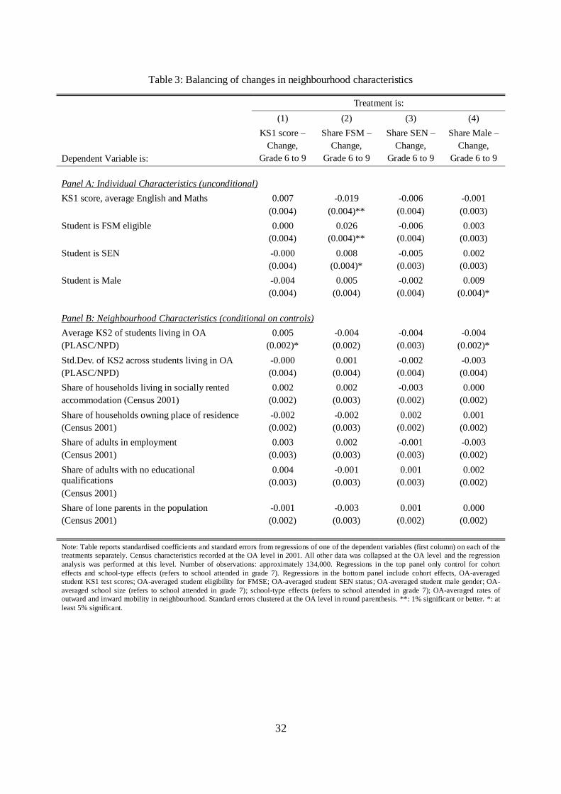
32

Table 3: Balancing of changes in neighbourhood characteristics

Treatment is:

(1) (2) (3) (4)

Dependent Variable is:

KS1 score –

Change,

Grade 6 to 9

Share FSM –

Change,

Grade 6 to 9

Share SEN –

Change,

Grade 6 to 9

Share Male –

Change,

Grade 6 to 9

Panel A: Individual Characteristics (unconditional)

KS1 score, average English and Maths 0.007

(0.004)

-0.019

(0.004)**

-0.006

(0.004)

-0.001

(0.003)

Student is FSM eligible 0.000

(0.004)

0.026

(0.004)**

-0.006

(0.004)

0.003

(0.003)

Student is SEN -0.000

(0.004)

0.008

(0.004)*

-0.005

(0.003)

0.002

(0.003)

Student is Male -0.004

(0.004)

0.005

(0.004)

-0.002

(0.004)

0.009

(0.004)*

Panel B: Neighbourhood Characteristics (conditional on controls)

Average KS2 of students living in OA

(PLASC/NPD)

0.005

(0.002)*

-0.004

(0.002)

-0.004

(0.003)

-0.004

(0.002)*

Std.Dev. of KS2 across students living in OA

(PLASC/NPD)

-0.000

(0.004)

0.001

(0.004)

-0.002

(0.004)

-0.003

(0.004)

Share of households living in socially rented

accommodation (Census 2001)

0.002

(0.002)

0.002

(0.003)

-0.003

(0.002)

0.000

(0.002)

Share of households owning place of residence

(Census 2001)

-0.002

(0.002)

-0.002

(0.003)

0.002

(0.002)

0.001

(0.002)

Share of adults in employment

(Census 2001)

0.003

(0.003)

0.002

(0.003)

-0.001

(0.003)

-0.003

(0.002)

Share of adults with no educational qualifications

(Census 2001)

0.004

(0.003)

-0.001

(0.003)

0.001

(0.003)

0.002

(0.002)

Share of lone parents in the population

(Census 2001)

-0.001

(0.002)

-0.003

(0.003)

0.001

(0.002)

0.000

(0.002)

Note: Table reports standardised coefficients and standard errors from regressions of one of the dependent variables (first column) on each of the

treatments separately. Census characteristics recorded at the OA level in 2001. All other data was collapsed at the OA level and the regression

analysis was performed at this level. Number of observations: approximately 134,000. Regressions in the top panel only control for cohort

effects and school-type effects (refers to school attended in grade 7). Regressions in the bottom panel include cohort effects, OA-averaged

student KS1 test scores; OA-averaged student eligibility for FMSE; OA-averaged student SEN status; OA-averaged student male gender; OA-

averaged school size (refers to school attended in grade 7); school-type effects (refers to school attended in grade 7); OA-averaged rates of

outward and inward mobility in neighbourhood. Standard errors clustered at the OA level in round parenthesis. **: 1% significant or better. *: at

least 5% significant.

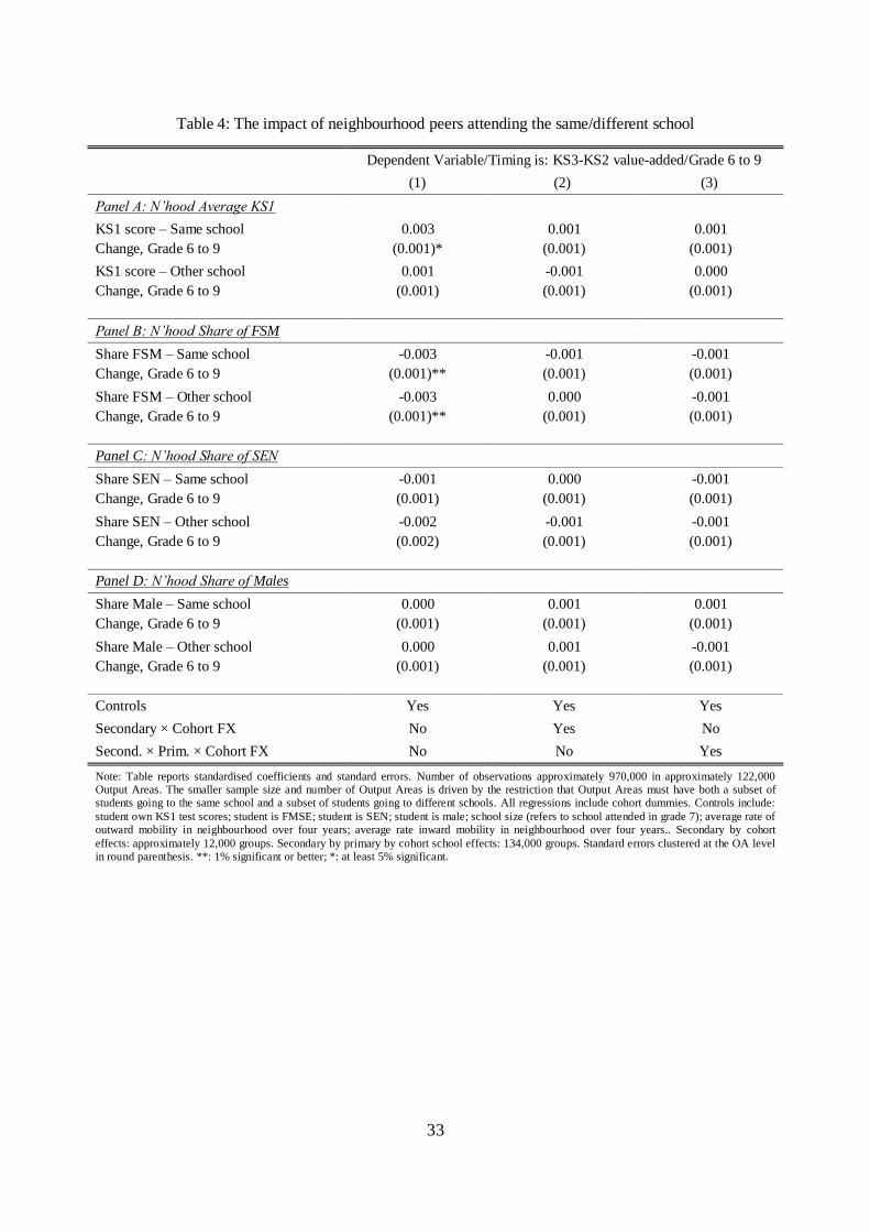
33

Table 4: The impact of neighbourhood peers attending the same/different school

Dependent Variable/Timing is: KS3-KS2 value-added/Grade 6 to 9

(1) (2) (3)

Panel A: N’hood Average KS1

KS1 score – Same school

Change, Grade 6 to 9

0.003

(0.001)*

0.001

(0.001)

0.001

(0.001)

KS1 score – Other school

Change, Grade 6 to 9

0.001

(0.001)

-0.001

(0.001)

0.000

(0.001)

Panel B: N’hood Share of FSM

Share FSM – Same school

Change, Grade 6 to 9

-0.003

(0.001)**

-0.001

(0.001)

-0.001

(0.001)

Share FSM – Other school

Change, Grade 6 to 9

-0.003

(0.001)**

0.000

(0.001)

-0.001

(0.001)

Panel C: N’hood Share of SEN

Share SEN – Same school

Change, Grade 6 to 9

-0.001

(0.001)

0.000

(0.001)

-0.001

(0.001)

Share SEN – Other school

Change, Grade 6 to 9

-0.002

(0.002)

-0.001

(0.001)

-0.001

(0.001)

Panel D: N’hood Share of Males

Share Male – Same school

Change, Grade 6 to 9

0.000

(0.001)

0.001

(0.001)

0.001

(0.001)

Share Male – Other school

Change, Grade 6 to 9

0.000

(0.001)

0.001

(0.001)

-0.001

(0.001)

Controls Yes Yes Yes

Secondary × Cohort FX No Yes No

Second. × Prim. × Cohort FX No No Yes

Note: Table reports standardised coefficients and standard errors. Number of observations approximately 970,000 in approximately 122,000

Output Areas. The smaller sample size and number of Output Areas is driven by the restriction that Output Areas must have both a subset of

students going to the same school and a subset of students going to different schools. All regressions include cohort dummies. Controls include:

student own KS1 test scores; student is FMSE; student is SEN; student is male; school size (refers to school attended in grade 7); average rate of

outward mobility in neighbourhood over four years; average rate inward mobility in neighbourhood over four years.. Secondary by cohort

effects: approximately 12,000 groups. Secondary by primary by cohort school effects: 134,000 groups. Standard errors clustered at the OA level

in round parenthesis. **: 1% significant or better; *: at least 5% significant.

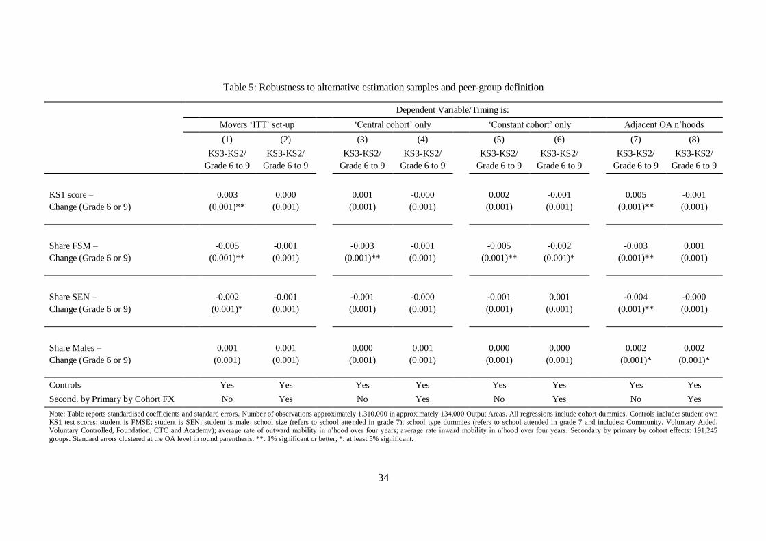
34

Table 5: Robustness to alternative estimation samples and peer-group definition

Dependent Variable/Timing is:

Movers „ITT‟ set-up „Central cohort‟ only „Constant cohort‟ only Adjacent OA n‟hoods

(1) (2) (3) (4) (5) (6) (7) (8)

KS3-KS2/

Grade 6 to 9

KS3-KS2/

Grade 6 to 9

KS3-KS2/

Grade 6 to 9

KS3-KS2/

Grade 6 to 9

KS3-KS2/

Grade 6 to 9

KS3-KS2/

Grade 6 to 9

KS3-KS2/

Grade 6 to 9

KS3-KS2/

Grade 6 to 9

KS1 score –

Change (Grade 6 or 9)

0.003

(0.001)**

0.000

(0.001)

0.001

(0.001)

-0.000

(0.001)

0.002

(0.001)

-0.001

(0.001)

0.005

(0.001)**

-0.001

(0.001)

Share FSM –

Change (Grade 6 or 9)

-0.005

(0.001)**

-0.001

(0.001)

-0.003

(0.001)**

-0.001

(0.001)

-0.005

(0.001)**

-0.002

(0.001)*

-0.003

(0.001)**

0.001

(0.001)

Share SEN –

Change (Grade 6 or 9)

-0.002

(0.001)*

-0.001

(0.001)

-0.001

(0.001)

-0.000

(0.001)

-0.001

(0.001)

0.001

(0.001)

-0.004

(0.001)**

-0.000

(0.001)

Share Males –

Change (Grade 6 or 9)

0.001

(0.001)

0.001

(0.001)

0.000

(0.001)

0.001

(0.001)

0.000

(0.001)

0.000

(0.001)

0.002

(0.001)*

0.002

(0.001)*

Controls Yes Yes Yes Yes Yes Yes Yes Yes

Second. by Primary by Cohort FX No Yes No Yes No Yes No Yes

Note: Table reports standardised coefficients and standard errors. Number of observations approximately 1,310,000 in approximately 134,000 Output Areas. All regressions include cohort dummies. Controls include: student own

KS1 test scores; student is FMSE; student is SEN; student is male; school size (refers to school attended in grade 7); school type dummies (refers to school attended in grade 7 and includes: Community, Voluntary Aided,

Voluntary Controlled, Foundation, CTC and Academy); average rate of outward mobility in n‟hood over four years; average rate inward mobility in n‟hood over four years. Secondary by primary by cohort effects: 191,245

groups. Standard errors clustered at the OA level in round parenthesis. **: 1% significant or better; *: at least 5% significant.

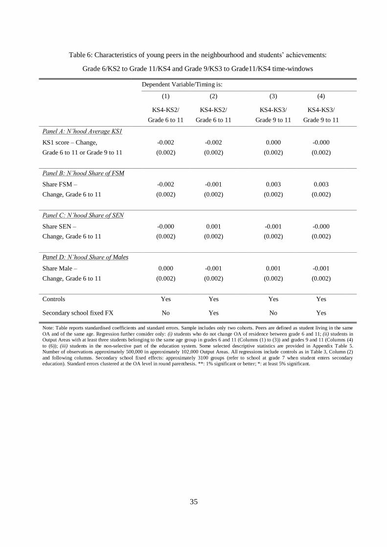
35

Table 6: Characteristics of young peers in the neighbourhood and students‟ achievements:

Grade 6/KS2 to Grade 11/KS4 and Grade 9/KS3 to Grade11/KS4 time-windows

Dependent Variable/Timing is:

(1) (2) (3) (4)

KS4-KS2/

Grade 6 to 11

KS4-KS2/

Grade 6 to 11

KS4-KS3/

Grade 9 to 11

KS4-KS3/

Grade 9 to 11

Panel A: N’hood Average KS1

KS1 score – Change,

Grade 6 to 11 or Grade 9 to 11

-0.002

(0.002)

-0.002

(0.002)

0.000

(0.002)

-0.000

(0.002)

Panel B: N’hood Share of FSM

Share FSM –

Change, Grade 6 to 11

-0.002

(0.002)

-0.001

(0.002)

0.003

(0.002)

0.003

(0.002)

Panel C: N’hood Share of SEN

Share SEN –

Change, Grade 6 to 11

-0.000

(0.002)

0.001

(0.002)

-0.001

(0.002)

-0.000

(0.002)

Panel D: N’hood Share of Males

Share Male –

Change, Grade 6 to 11

0.000

(0.002)

-0.001

(0.002)

0.001

(0.002)

-0.001

(0.002)

Controls Yes Yes Yes Yes

Secondary school fixed FX No Yes No Yes

Note: Table reports standardised coefficients and standard errors. Sample includes only two cohorts. Peers are defined as student living in the same

OA and of the same age. Regression further consider only: (i) students who do not change OA of residence between grade 6 and 11; (ii) students in

Output Areas with at least three students belonging to the same age group in grades 6 and 11 (Columns (1) to (3)) and grades 9 and 11 (Columns (4)

to (6)); (iii) students in the non-selective part of the education system. Some selected descriptive statistics are provided in Appendix Table 5.

Number of observations approximately 500,000 in approximately 102,000 Output Areas. All regressions include controls as in Table 3, Column (2)

and following columns. Secondary school fixed effects: approximately 3100 groups (refer to school at grade 7 when student enters secondary

education). Standard errors clustered at the OA level in round parenthesis. **: 1% significant or better; *: at least 5% significant.

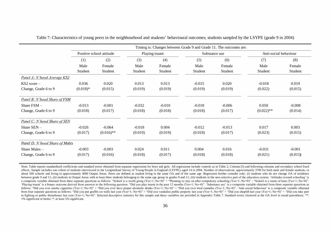
36

Table 7: Characteristics of young peers in the neighbourhood and students‟ behavioural outcomes; students sampled by the LSYPE (grade 9 in 2004)

Timing is: Changes between Grade 9 and Grade 11. The outcomes are:

Positive school attitude Playing truant Substance use Anti-social behaviour

(1) (2) (3) (4) (5) (6) (7) (8)

Male

Student

Female

Student

Male

Student

Female

Student

Male

Student

Female

Student

Male

Student

Female

Student

Panel A: N’hood Average KS2

KS2 score –

Change, Grade 6 to 9

0.036

(0.018)*

0.020

(0.015)

0.013

(0.019)

0.013

(0.019)

-0.015

(0.019)

0.020

(0.019)

-0.018

(0.022)

0.019

(0.015)

Panel B: N’hood Share of FSM

Share FSM –

Change, Grade 6 to 9

-0.013

(0.018)

-0.001

(0.017)

-0.032

(0.018)

-0.010

(0.018)

-0.018

(0.018)

-0.006

(0.017)

0.050

(0.022)**

-0.008

(0.014)

Panel C: N’hood Share of SEN

Share SEN –

Change, Grade 6 to 9

-0.026

(0.017)

-0.064

(0.016)**

-0.018

(0.019)

0.004

(0.019)

-0.012

(0.018)

-0.013

(0.017)

0.017

(0.023)

0.003

(0.015)

Panel D: N’hood Share of Males

Share Males –

Change, Grade 6 to 9

-0.003

(0.017)

-0.003

(0.016)

0.024

(0.018)

0.011

(0.017)

0.004

(0.018)

0.016

(0.018)

-0.031

(0.021)

-0.001

(0.015)

Note: Table reports standardised coefficients and standard errors obtained from separate regressions for boys and girls. All regressions include controls as in Table 2, Column (5) and following columns and secondary school fixed

effects. Sample includes one cohort of students interviewed in the Longitudinal Survey of Young People in England (LSYPE), aged 14 in 2004. Number of observations: approximately 3700 for both male and female students, in

about 500 schools and living in approximately 4000 Output Areas. Peers are defined as student living in the same OA and of the same age. Regression further consider only: (i) students who do not change OA of residence

between grade 9 and 11; (ii) students in Output Areas with at least three students belonging to the same age group in grades 9 and 11; (iii) students in the non-selective part of the education system. „Attitudes toward schooling‟ is

a composite variable obtained from three separate questions as follows: “School is a worth going (Yes=1; No=0)” + “Planning to stay on after compulsory schooling (Yes=1; No=0)” - “School is a waste of time (Yes=1; No=0)”.

„Playing truant‟ is a binary outcome derived from answers to the following question: “Did you play truant in the past 12 months (Yes=1; No=0)”. „Substance use‟ is a composite variable obtained from three separate questions as

follows: “Did you ever smoke cigarettes (Yes=1; No=0)” + “Did you ever have proper alcoholic drinks (Yes=1; No=0)” + “Did you ever tried cannabis (Yes=1; No=0)”. „Anti -social behaviour‟ is a composite variable obtained

from four separate questions as follows: “Did you put graffiti on walls last year (Yes=1; No=0)” + “Did you vandalise public property last year (Yes=1; No=0)” + “Did you shoplift last year (Yes=1; No=0)” + “Did you take part

in fighting or public disturbance last year (Yes=1; No=0)”. Selected descriptive statistics for this sample and these variables are provided in Appendix Table 7. Standard errors clustered at the OA level in round parenthesis. **:

1% significant or better; *: at least 5% significant.

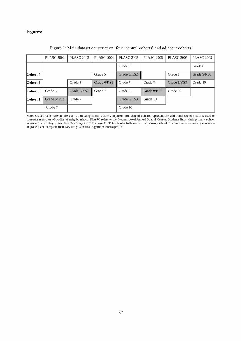
37

Figures:

Figure 1: Main dataset construction; four „central cohorts‟ and adjacent cohorts

PLASC 2002 PLASC 2003 PLASC 2004 PLASC 2005 PLASC 2006 PLASC 2007 PLASC 2008

Grade 5 Grade 8

Cohort 4 Grade 5 Grade 6/KS2 Grade 8 Grade 9/KS3

Cohort 3 Grade 5 Grade 6/KS2 Grade 7 Grade 8 Grade 9/KS3 Grade 10

Cohort 2 Grade 5 Grade 6/KS2 Grade 7 Grade 8 Grade 9/KS3 Grade 10

Cohort 1 Grade 6/KS2 Grade 7 Grade 9/KS3 Grade 10

Grade 7 Grade 10

Note: Shaded cells refer to the estimation sample; immediately adjacent non-shaded cohorts represent the additional set of students used to

construct measures of quality of neighbourhood. PLASC refers to the Student Level Annual School Census. Students finish their primary school

in grade 6 when they sit for their Key Stage 2 (KS2) at age 11. Thick border indicates end of primary school. Students enter secondary education

in grade 7 and complete their Key Stage 3 exams in grade 9 when aged 14.

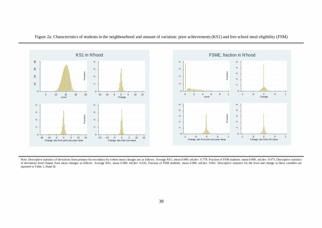
38

Figure 2a: Characteristics of students in the neighbourhood and amount of variation: prior achievements (KS1) and free school meal eligibility (FSM)

0

.02

.04

.06

.08

Fra

ction

5 10 15 20 25Level

0.1

.2.3

.4

Fra

ctio

n

-15 -10 -5 0 5 10 15Change

0.1

.2.3

.4

Fra

ction

-15 -10 -5 0 5 10 15

Change, dev.from prim-sec-year mean

0.1

.2.3

.4

Fra

ctio

n

-15 -10 -5 0 5 10 15

Change, dev.from OA mean

KS1 in N'hood

0.1

.2.3

.4

Fra

ction

0 .2 .4 .6 .8 1Level

0.1

.2.3

.4.5

Fra

ctio

n

-1 -.5 0 .5 1Change

0.1

.2.3

.4.5

Fra

ction

-1 -.5 0 .5 1

Change, dev.from prim-sec-year mean

0.1

.2.3

.4.5

Fra

ctio

n

-1 -.5 0 .5 1

Change, dev.from OA mean

FSME, fraction in N'hood

Note: Descriptive statistics of deviations from primary-by-secondary-by-cohort mean changes are as follows. Average KS1, mean 0.000; std.dev. 0.778. Fraction of FSM students: mean 0.000, std.dev. 0.073. Descriptive statistics

of deviations from Output Area mean changes as follows. Average KS1, mean 0.000; std.dev. 0.632. Fraction of FSM students: mean 0.000, std.dev. 0.061. Descriptive statistics for the level and change in these variables are

reported in Table 1, Panel B.

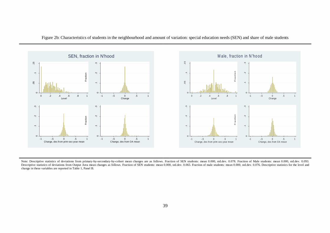
39

Figure 2b: Characteristics of students in the neighbourhood and amount of variation: special education needs (SEN) and share of male students

0

.05

.1.1

5

Fra

ction

0 .2 .4 .6 .8 1Level

0.1

.2.3

Fra

ctio

n

-1 -.5 0 .5 1Change

0.1

.2.3

Fra

ction

-1 -.5 0 .5 1

Change, dev.from prim-sec-year mean

0.1

.2.3

Fra

ctio

n

-1 -.5 0 .5 1

Change, dev.from OA mean

SEN, fraction in N'hood

0

.0

5.1

.1

5

Fra

ctio

n

0 .2 .4 .6 .8 1Le ve l

0.1

.2

.3

Fra

ctio

n

- 1 - .5 0 .5 1C h an ge

0.1

.2

.3

Fra

ctio

n

- 1 - .5 0 .5 1

C h an ge , d ev .fro m pr im -se c -ye ar m e an

0.1

.2

.3

Fra

ctio

n

- 1 - .5 0 .5 1

C ha ng e, d ev .from O A m e a n

M ale, frac tion in N 'ho od

Note: Descriptive statistics of deviations from primary-by-secondary-by-cohort mean changes are as follows. Fraction of SEN students: mean 0.000, std.dev. 0.078. Fraction of Male students: mean 0.000, std.dev. 0.093.

Descriptive statistics of deviations from Output Area mean changes as follows. Fraction of SEN students: mean 0.000, std.dev. 0.065. Fraction of male students: mean 0.000, std.dev. 0.076. Descriptive statistics for the level and

change in these variables are reported in Table 1, Panel B.

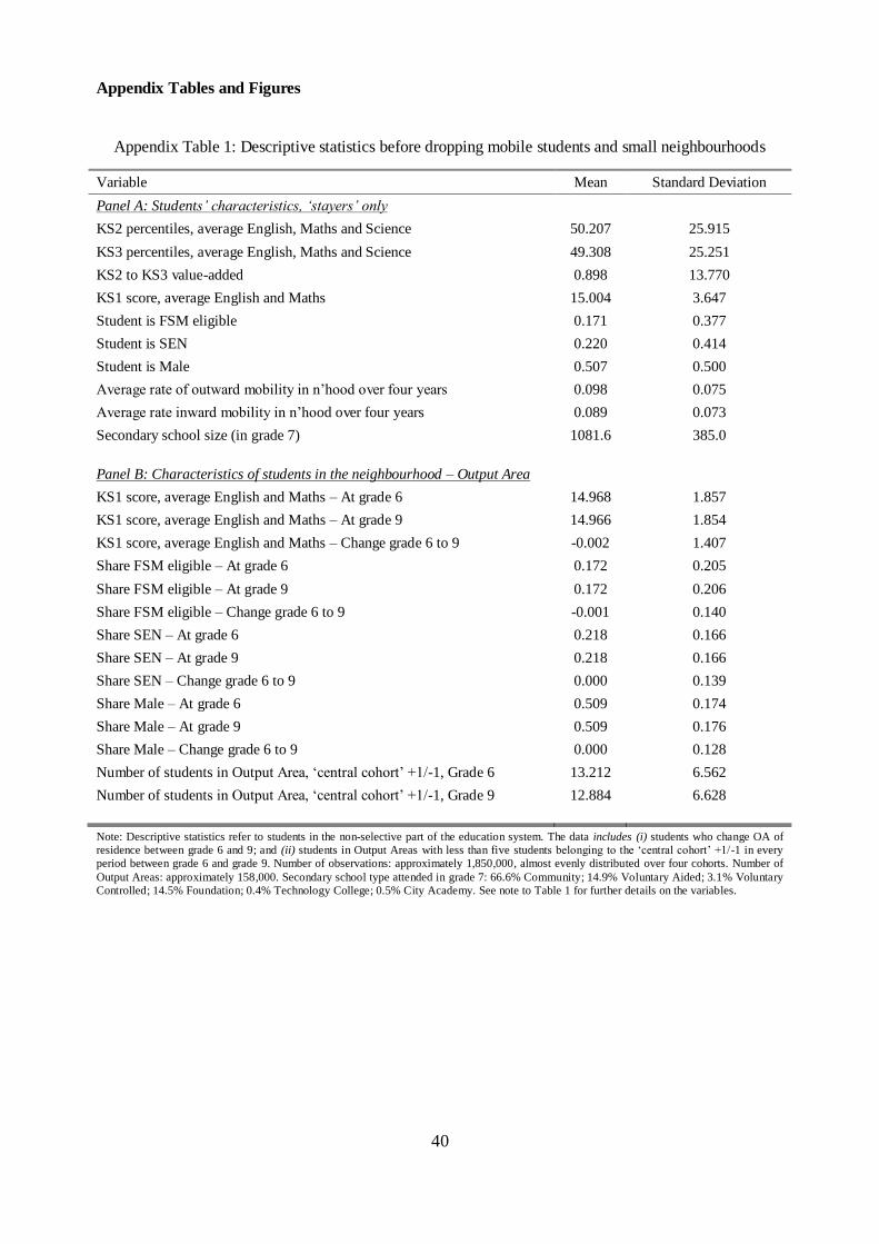
40

Appendix Tables and Figures

Appendix Table 1: Descriptive statistics before dropping mobile students and small neighbourhoods

Variable Mean Standard Deviation

Panel A: Students’ characteristics, ‘stayers’ only

KS2 percentiles, average English, Maths and Science 50.207 25.915

KS3 percentiles, average English, Maths and Science 49.308 25.251

KS2 to KS3 value-added 0.898 13.770

KS1 score, average English and Maths 15.004 3.647

Student is FSM eligible 0.171 0.377

Student is SEN 0.220 0.414

Student is Male 0.507 0.500

Average rate of outward mobility in n‟hood over four years 0.098 0.075

Average rate inward mobility in n‟hood over four years 0.089 0.073

Secondary school size (in grade 7) 1081.6 385.0

Panel B: Characteristics of students in the neighbourhood – Output Area

KS1 score, average English and Maths – At grade 6 14.968 1.857

KS1 score, average English and Maths – At grade 9 14.966 1.854

KS1 score, average English and Maths – Change grade 6 to 9 -0.002 1.407

Share FSM eligible – At grade 6 0.172 0.205

Share FSM eligible – At grade 9 0.172 0.206

Share FSM eligible – Change grade 6 to 9 -0.001 0.140

Share SEN – At grade 6 0.218 0.166

Share SEN – At grade 9 0.218 0.166

Share SEN – Change grade 6 to 9 0.000 0.139

Share Male – At grade 6 0.509 0.174

Share Male – At grade 9 0.509 0.176

Share Male – Change grade 6 to 9 0.000 0.128

Number of students in Output Area, „central cohort‟ +1/-1, Grade 6 13.212 6.562

Number of students in Output Area, „central cohort‟ +1/-1, Grade 9 12.884 6.628

Note: Descriptive statistics refer to students in the non-selective part of the education system. The data includes (i) students who change OA of

residence between grade 6 and 9; and (ii) students in Output Areas with less than five students belonging to the „central cohort‟ +1/-1 in every

period between grade 6 and grade 9. Number of observations: approximately 1,850,000, almost evenly distributed over four cohorts. Number of

Output Areas: approximately 158,000. Secondary school type attended in grade 7: 66.6% Community; 14.9% Voluntary Aided; 3.1% Voluntary

Controlled; 14.5% Foundation; 0.4% Technology College; 0.5% City Academy. See note to Table 1 for further details on the variables.

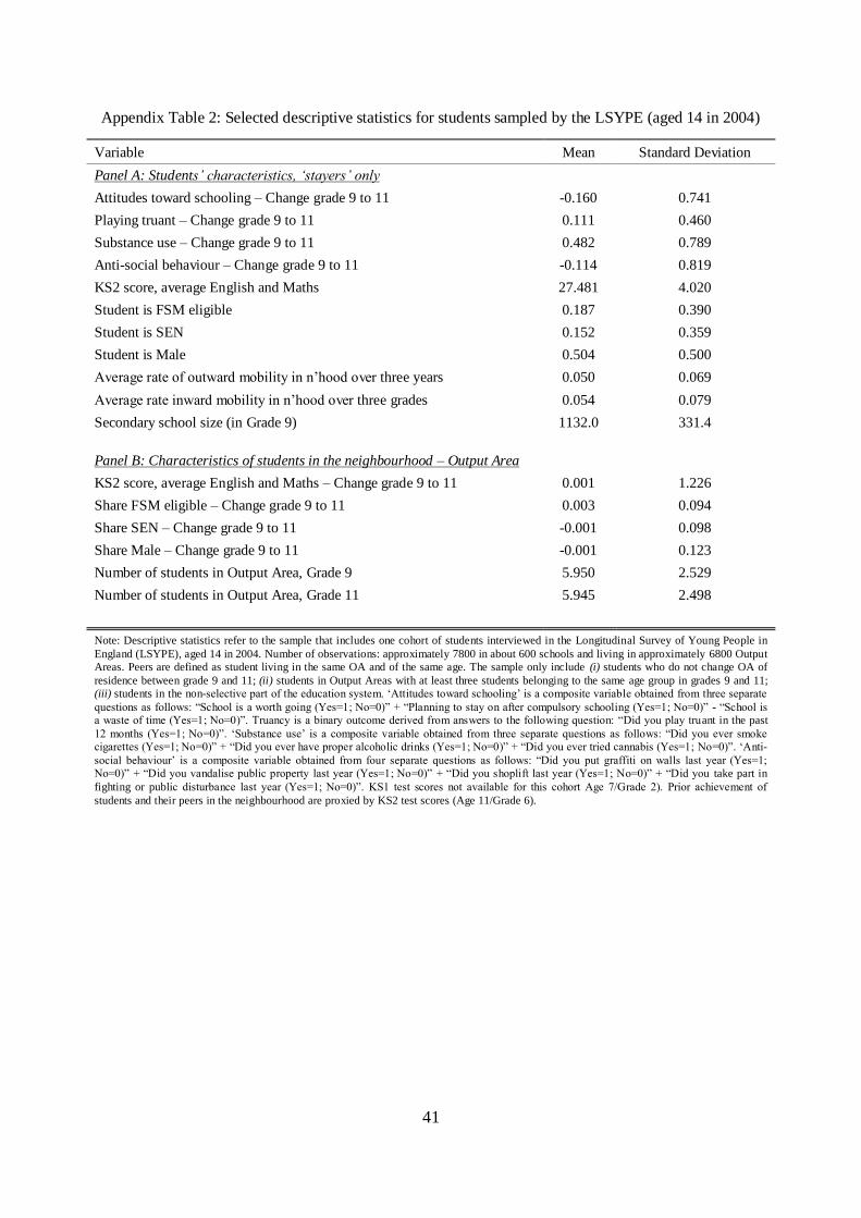
41

Appendix Table 2: Selected descriptive statistics for students sampled by the LSYPE (aged 14 in 2004)

Variable Mean Standard Deviation

Panel A: Students’ characteristics, ‘stayers’ only

Attitudes toward schooling – Change grade 9 to 11 -0.160 0.741

Playing truant – Change grade 9 to 11 0.111 0.460

Substance use – Change grade 9 to 11 0.482 0.789

Anti-social behaviour – Change grade 9 to 11 -0.114 0.819

KS2 score, average English and Maths 27.481 4.020

Student is FSM eligible 0.187 0.390

Student is SEN 0.152 0.359

Student is Male 0.504 0.500

Average rate of outward mobility in n‟hood over three years 0.050 0.069

Average rate inward mobility in n‟hood over three grades 0.054 0.079

Secondary school size (in Grade 9) 1132.0 331.4

Panel B: Characteristics of students in the neighbourhood – Output Area

KS2 score, average English and Maths – Change grade 9 to 11 0.001 1.226

Share FSM eligible – Change grade 9 to 11 0.003 0.094

Share SEN – Change grade 9 to 11 -0.001 0.098

Share Male – Change grade 9 to 11 -0.001 0.123

Number of students in Output Area, Grade 9 5.950 2.529

Number of students in Output Area, Grade 11 5.945 2.498

Note: Descriptive statistics refer to the sample that includes one cohort of students interviewed in the Longitudinal Survey of Young People in

England (LSYPE), aged 14 in 2004. Number of observations: approximately 7800 in about 600 schools and living in approximately 6800 Output

Areas. Peers are defined as student living in the same OA and of the same age. The sample only include (i) students who do not change OA of

residence between grade 9 and 11; (ii) students in Output Areas with at least three students belonging to the same age group in grades 9 and 11;

(iii) students in the non-selective part of the education system. „Attitudes toward schooling‟ is a composite variable obtained from three separate

questions as follows: “School is a worth going (Yes=1; No=0)” + “Planning to stay on after compulsory schooling (Yes=1; No=0)” - “School is

a waste of time (Yes=1; No=0)”. Truancy is a binary outcome derived from answers to the following question: “Did you play truant in the past

12 months (Yes=1; No=0)”. „Substance use‟ is a composite variable obtained from three separate questions as follows: “Did you ever smoke

cigarettes (Yes=1; No=0)” + “Did you ever have proper alcoholic drinks (Yes=1; No=0)” + “Did you ever tried cannabis (Yes=1; No=0)”. „Anti-

social behaviour‟ is a composite variable obtained from four separate questions as follows: “Did you put graffiti on walls last year (Yes=1;

No=0)” + “Did you vandalise public property last year (Yes=1; No=0)” + “Did you shoplift last year (Yes=1; No=0)” + “Did you take part in

fighting or public disturbance last year (Yes=1; No=0)”. KS1 test scores not available for this cohort Age 7/Grade 2). Prior achievement of

students and their peers in the neighbourhood are proxied by KS2 test scores (Age 11/Grade 6).

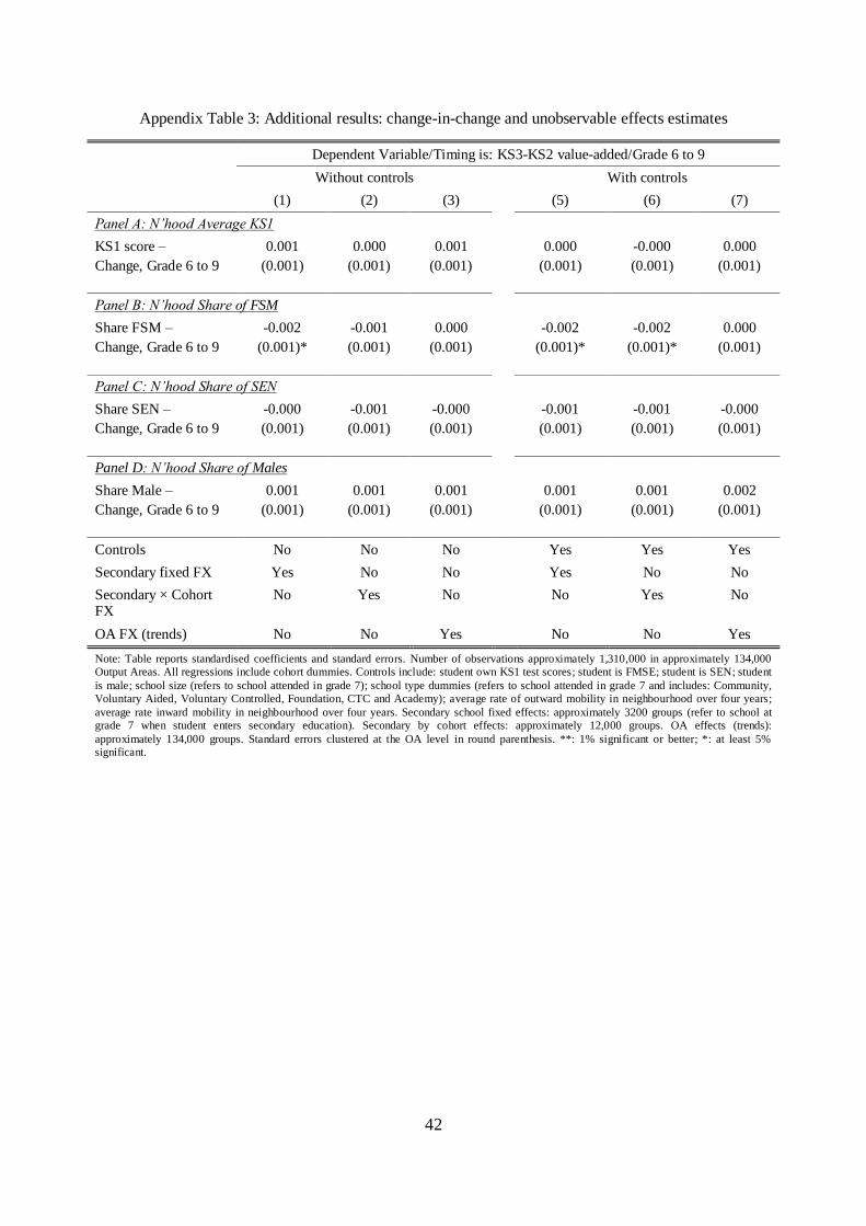
42

Appendix Table 3: Additional results: change-in-change and unobservable effects estimates

Dependent Variable/Timing is: KS3-KS2 value-added/Grade 6 to 9

Without controls With controls

(1) (2) (3) (5) (6) (7)

Panel A: N’hood Average KS1

KS1 score –

Change, Grade 6 to 9

0.001

(0.001)

0.000

(0.001)

0.001

(0.001)

0.000

(0.001)

-0.000

(0.001)

0.000

(0.001)

Panel B: N’hood Share of FSM

Share FSM –

Change, Grade 6 to 9

-0.002

(0.001)*

-0.001

(0.001)

0.000

(0.001)

-0.002

(0.001)*

-0.002

(0.001)*

0.000

(0.001)

Panel C: N’hood Share of SEN

Share SEN –

Change, Grade 6 to 9

-0.000

(0.001)

-0.001

(0.001)

-0.000

(0.001)

-0.001

(0.001)

-0.001

(0.001)

-0.000

(0.001)

Panel D: N’hood Share of Males

Share Male –

Change, Grade 6 to 9

0.001

(0.001)

0.001

(0.001)

0.001

(0.001)

0.001

(0.001)

0.001

(0.001)

0.002

(0.001)

Controls No No No Yes Yes Yes

Secondary fixed FX Yes No No Yes No No

Secondary × Cohort FX

No Yes No No Yes No

OA FX (trends) No No Yes No No Yes

Note: Table reports standardised coefficients and standard errors. Number of observations approximately 1,310,000 in approximately 134,000

Output Areas. All regressions include cohort dummies. Controls include: student own KS1 test scores; student is FMSE; student is SEN; student

is male; school size (refers to school attended in grade 7); school type dummies (refers to school attended in grade 7 and includes: Community,

Voluntary Aided, Voluntary Controlled, Foundation, CTC and Academy); average rate of outward mobility in neighbourhood over four years;

average rate inward mobility in neighbourhood over four years. Secondary school fixed effects: approximately 3200 groups (refer to school at

grade 7 when student enters secondary education). Secondary by cohort effects: approximately 12,000 groups. OA effects (trends):

approximately 134,000 groups. Standard errors clustered at the OA level in round parenthesis. **: 1% significant or better; *: at least 5%

significant.

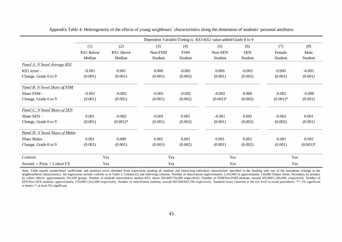
43

Appendix Table 4: Heterogeneity of the effects of young neighbours‟ characteristics along the dimension of students‟ personal attributes

Dependent Variable/Timing is: KS3-KS2 value-added/Grade 6 to 9

(1) (2) (3) (4) (5) (6) (7) (8)

KS1 Below

Median

KS1 Above

Median

Non-FSM

Student

FSM

Student

Non-SEN

Student

SEN

Student

Female

Student

Male

Student

Panel A: N’hood Average KS1

KS1 score –

Change, Grade 6 to 9

-0.001

(0.001)

0.001

(0.001)

0.000

(0.001)

-0.001

(0.002)

0.000

(0.001)

-0.003

(0.002)

0.000

(0.001)

-0.001

(0.001)

Panel B: N’hood Share of FSM

Share FSM –

Change, Grade 6 to 9

-0.001

(0.001)

-0.002

(0.002)

-0.001

(0.001)

-0.002

(0.002)

-0.002

(0.001)*

0.000

(0.002)

-0.002

(0.001)*

-0.000

(0.001)

Panel C: N’hood Share of SEN

Share SEN –

Change, Grade 6 to 9

0.001

(0.001)

-0.002

(0.001)*

-0.001

(0.001)

0.001

(0.002)

-0.001

(0.001)

0.002

(0.002)

-0.002

(0.002)

0.001

(0.001)

Panel D: N’hood Share of Males

Share Males –

Change, Grade 6 to 9

0.001

(0.001)

0.000

(0.001)

0.001

(0.001)

0.001

(0.002)

0.001

(0.001)

0.001

(0.002)

-0.001

(0.001)

0.002

(0.001)*

Controls Yes Yes Yes Yes

Second. × Prim. × Cohort FX Yes Yes Yes Yes

Note: Table reports standardised coefficients and standard errors obtained from regressions pooling all students and interacting individual characteristic specified in the heading with one of the treatments (change in the

neighbourhood characteristic). All regressions include controls as in Table 3, Column (2) and following columns. Number of observations approximately 1,310,000 in approximately 134,000 Output Areas. Secondary by primary

by cohort effects: approximately 191,000 groups. Number of students above/below median KS1: about 582,000/726,000 respectively. Number of FSM/Non-FSM students: around 203,000/1,106,000, respectively. Number of

SEN/Non-SEN students: approximately 279,000/1,031,000 respectively. Number of male/female students: around 665,500/643,700 respectively. Standard errors clustered at the OA level in round parenthesis. **: 1% significant

or better; *: at least 5% significant.

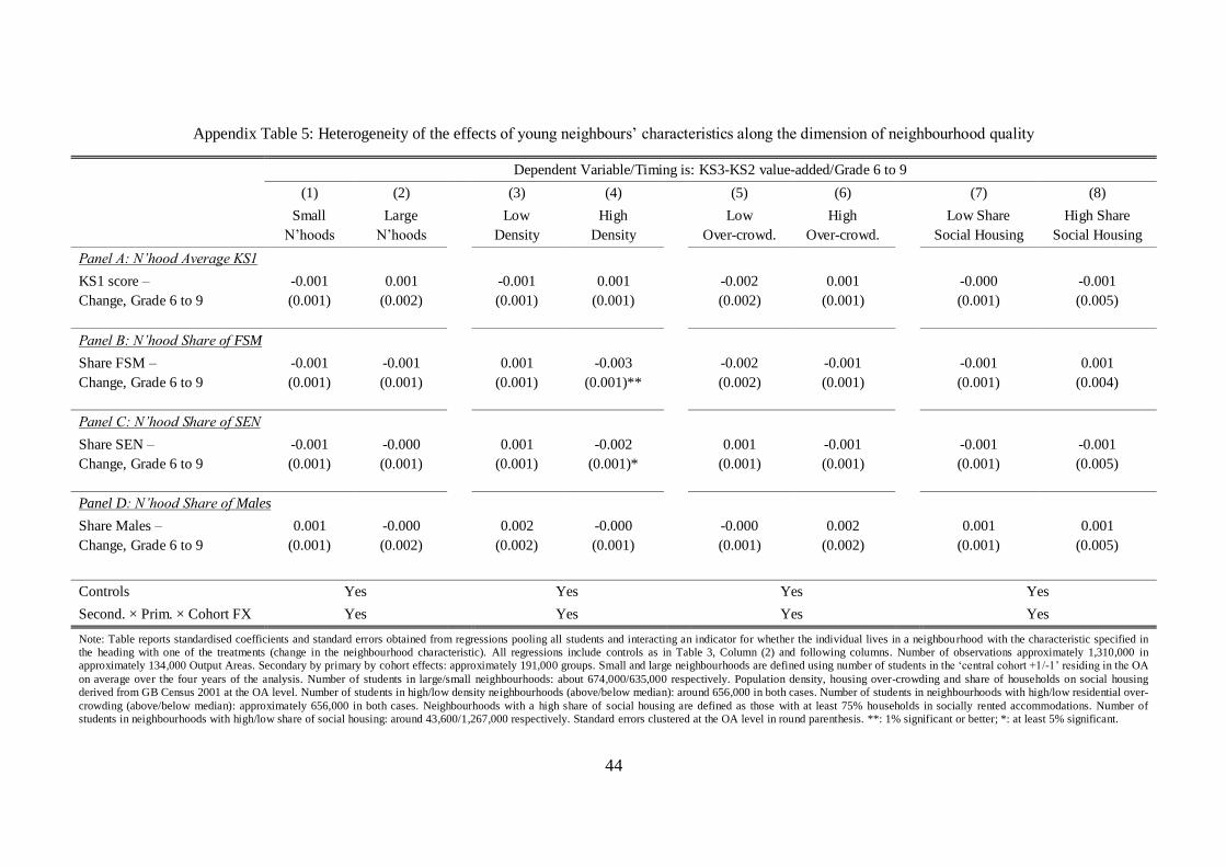
44

Appendix Table 5: Heterogeneity of the effects of young neighbours‟ characteristics along the dimension of neighbourhood quality

Dependent Variable/Timing is: KS3-KS2 value-added/Grade 6 to 9

(1) (2) (3) (4) (5) (6) (7) (8)

Small

N‟hoods

Large

N‟hoods

Low

Density

High

Density

Low

Over-crowd.

High

Over-crowd.

Low Share

Social Housing

High Share

Social Housing

Panel A: N’hood Average KS1

KS1 score –

Change, Grade 6 to 9

-0.001

(0.001)

0.001

(0.002)

-0.001

(0.001)

0.001

(0.001)

-0.002

(0.002)

0.001

(0.001)

-0.000

(0.001)

-0.001

(0.005)

Panel B: N’hood Share of FSM

Share FSM –

Change, Grade 6 to 9

-0.001

(0.001)

-0.001

(0.001)

0.001

(0.001)

-0.003

(0.001)**

-0.002

(0.002)

-0.001

(0.001)

-0.001

(0.001)

0.001

(0.004)

Panel C: N’hood Share of SEN

Share SEN –

Change, Grade 6 to 9

-0.001

(0.001)

-0.000

(0.001)

0.001

(0.001)

-0.002

(0.001)*

0.001

(0.001)

-0.001

(0.001)

-0.001

(0.001)

-0.001

(0.005)

Panel D: N’hood Share of Males

Share Males –

Change, Grade 6 to 9

0.001

(0.001)

-0.000

(0.002)

0.002

(0.002)

-0.000

(0.001)

-0.000

(0.001)

0.002

(0.002)

0.001

(0.001)

0.001

(0.005)

Controls Yes Yes Yes Yes

Second. × Prim. × Cohort FX Yes Yes Yes Yes

Note: Table reports standardised coefficients and standard errors obtained from regressions pooling all students and interacting an indicator for whether the individual lives in a neighbourhood with the characteristic specified in

the heading with one of the treatments (change in the neighbourhood characteristic). All regressions include controls as in Table 3, Column (2) and following columns. Number of observations approximately 1,310,000 in

approximately 134,000 Output Areas. Secondary by primary by cohort effects: approximately 191,000 groups. Small and large neighbourhoods are defined using number of students in the „central cohort +1/-1‟ residing in the OA

on average over the four years of the analysis. Number of students in large/small neighbourhoods: about 674,000/635,000 respectively. Population density, housing over-crowding and share of households on social housing

derived from GB Census 2001 at the OA level. Number of students in high/low density neighbourhoods (above/below median): around 656,000 in both cases. Number of students in neighbourhoods with high/low residential over-

crowding (above/below median): approximately 656,000 in both cases. Neighbourhoods with a high share of social housing are defined as those with at least 75% households in socially rented accommodations. Number of students in neighbourhoods with high/low share of social housing: around 43,600/1,267,000 respectively. Standard errors clustered at the OA level in round parenthesis. **: 1% significant or better; *: at least 5% significant.

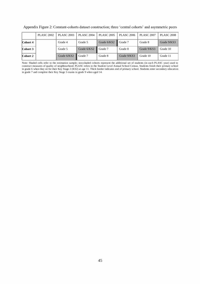
45

Appendix Figure 2: Constant-cohorts dataset construction; three „central cohorts‟ and asymmetric peers

PLASC 2002 PLASC 2003 PLASC 2004 PLASC 2005 PLASC 2006 PLASC 2007 PLASC 2008

Cohort 4 Grade 4 Grade 5 Grade 6/KS2 Grade 7 Grade 8 Grade 9/KS3

Cohort 3 Grade 5 Grade 6/KS2 Grade 7 Grade 8 Grade 9/KS3 Grade 10

Cohort 2 Grade 6/KS2 Grade 7 Grade 8 Grade 9/KS3 Grade 10 Grade 11

Note: Shaded cells refer to the estimation sample; non-shaded cohorts represent the additional set of students (in each PLASC year) used to

construct measures of quality of neighbourhood. PLASC refers to the Student Level Annual School Census. Students finish their primary school

in grade 6 when they sit for their Key Stage 2 (KS2) at age 11. Thick border indicates end of primary school. Students enter secondary education

in grade 7 and complete their Key Stage 3 exams in grade 9 when aged 14.