EVIDENCE FOR HIERARCHICAL STRUCTURING AND LARGE-SCALE

CONNECTIVITY IN EASTERN PACIFIC OLIVE RIDLEY SEA TURTLES

(LEPIDOCHELYS OLIVACEA) by

Ian M. Silver-Gorges

A Thesis

Submitted to the Faculty of Purdue University

In Partial Fulfillment of the Requirements for the degree of

Master of Science

Department of Biology

Fort Wayne, Indiana

May 2019

2

THE PURDUE UNIVERSITY GRADUATE SCHOOL

STATEMENT OF COMMITTEE APPROVAL

Dr. Frank V. Paladino, Chair

Department of Biology

Dr. Mark Jordan

Department of Biology

Dr. Tanya Soule

Department of Biology

Approved by:

Dr. Jordan M. Marshall

Head of the Graduate Program

3

ACKNOWLEDGMENTS

Immediate and highest thanks to Dr. Paladino for providing me with the opportunity to

grow as a person, to begin and develop as a scientist, and to have truly unparalleled experiences

conducting sea turtle research abroad. I will never forget your generosity and support. You

allowed me to follow my own interests, which has provided me with the skills and experience I

need to conduct research that truly aligns with my academic interests. Thank you, Frank.

Immense gratitude to Dr. Jordan, my often daily molecular ecology consultant. Thank you for

your constant guidance and support through the dense weeds of molecular ecology, from

experimental design (sometimes on the fly) through PCR and analysis after analysis after

analysis. Your encouragement was always timely and often what I needed to reach the next step.

Thanks to Dr. Soule as well, for providing prompt, thorough, and constructive feedback on

abstracts, posters, and, of course, manuscripts that were never submitted. You have helped me

elevate my scientific communication that much closer to what is expected of career researchers.

Thank you to Julianne Koval, whose shoulders I am standing on and whose friendship

and baby-visits have enriched my time at PFW. To Dar Bender, Colleen Krohn, Arlis Lamaster,

Bruce Arnold, and everyone else who helps the Biology department function, thank you for so

much. You have been integral to my success by helping me with anything and everything I have

needed every day for the past two years.

I send my thanks and encouragement to my friends and fellow PFW Biology graduate

students, without whom I would be lost. Emma “Erma” Mettler, Quintin “Qeenteen”

Bergman, Adam “Big Baby” Yaney-Keller, and Liz Cubberly have been absolute rocks of

support when I have needed them, and perhaps more importantly helped (and pressured) me to

find time to have fun and let off steam. From day 1 it was easy to be myself around these kind,

intelligent, and overall incredible people.

I would not be the student or person I am without incredible mentors. Drs. Cullen and

Peters at Oberlin College pushed me to become a better student and scientist, and fostered my

interest in molecular biology and genetics. Dr. Mariana Fuentes has supported my ideas and

engaged with me since 2016. Her guidance and support, and the opportunities she has given me,

be it inviting me to field work, serving as a reference, or providing guidance when designing and

implementing projects, has meant so much to my personal happiness and growth and has

4

supplemented my work at PFW. I cannot wait to begin working with her in earnest in the fall as

her PhD student. Dr. Matthew Godfrey opened the door to sea turtle research for me, and gave

me the space and resources to start building my career as a student. Dr. Kristin Arend provided

me with my first independent research experience in 2014, and has remained a mentor since

then. She helped me develop skills that I am benefitting from as a graduate student and her

advice and support have helped me get to where I am.

Dr. Carole Baldwin took me on as an undergraduate in 2012, and then again in 2013 and

2014, and finally for a year in 2016-2017. She showed me what it was to be a scientist, and

through her employ I developed some of the most integral organizational skills needed by any

scientist while honing my reef fish ID skills. Her trust and support pushed me along a path

towards professional marine biology. For all of the winter term and summer projects; for

supporting me with a job after college and after an operation prevented me from taking a

different job; for incredible experiences in Bonaire and at NHB; for all of the recommendations

and mentorship, thank you. I hope other students are as lucky as I am to have had a

compassionate and brilliant mentor like you.

Finally, thank you Mom and Dad for pushing me and supporting me on a path towards

marine biology ever since I first played in a California tide pool. I know that everything you’ve

done has been to help me get to where I am to become who I am. I love you.

5

TABLE OF CONTENTS

Acknowledgments........................................................................................................................... 3

Table Of Contents ........................................................................................................................... 5

List of Tables .................................................................................................................................. 7

List Of Figures ................................................................................................................................ 8

ABSTRACT .................................................................................................................................... 9

INTRODUCTION ........................................................................................................................ 11

Sea Turtle Population Biology .................................................................................................. 11

Sea Turtle Population Genetics ................................................................................................. 12

Mitochondrial DNA .............................................................................................................. 12

Nuclear DNA ........................................................................................................................ 12

Genetic Analyses in Population Biology .................................................................................. 13

F and F-like Statistics and Analysis of Molecular Variance ................................................. 13

Bottleneck Analysis .............................................................................................................. 13

Relatedness Analysis ............................................................................................................ 14

Migration Analysis ................................................................................................................ 15

Genetic Distance Analysis .................................................................................................... 16

Population Inference ................................................................................................................. 16

Bayesian Inference ................................................................................................................ 16

Ordination ............................................................................................................................. 17

Olive Ridley Sea Turtles ........................................................................................................... 18

Global Population Biology ................................................................................................... 18

Eastern Pacific Population Biology ...................................................................................... 18

Study Questions ........................................................................................................................ 19

METHODS ................................................................................................................................... 21

NWCR mtDNA Analysis .......................................................................................................... 21

Microsatellite Amplification ..................................................................................................... 22

Analyses .................................................................................................................................... 22

F and F-like Statistics and Analysis of Molecular Variance ................................................. 22

Population Inference ............................................................................................................. 23

6

Genetic Distance Analysis .................................................................................................... 24

Bottleneck Analysis .............................................................................................................. 24

Relatedness Analysis ............................................................................................................ 25

Migration Analysis ................................................................................................................ 25

RESULTS ..................................................................................................................................... 27

Mitochondrial DNA Analysis ................................................................................................... 27

Summary of Nuclear DNA Results from Previous Studies ...................................................... 27

Population Inference in ETP ORs ............................................................................................. 28

Genetic Distance Analysis ........................................................................................................ 29

Bottleneck Analysis .................................................................................................................. 29

Relatedness Analysis ................................................................................................................ 30

Migration Analysis ................................................................................................................... 31

DISCUSSION ............................................................................................................................... 58

Overview ................................................................................................................................... 58

Question 1: Would mtDNA analysis support or refine population structure in NWCR and

ETP ORs?.......................................................................................................................... 58

Question 2: Would analysis of ETP OR nDNA elucidate substructuring within Mexican

and/or Central American populations? ............................................................................. 58

Question 3: Would DAPC produce cryptic clusters in both NWCR and ETP ORs? ....... 59

Question 4: What processes might be contributing to the formation of inferred

populations, and which inferred populations were best supported by multiple analyses? 59

Genetic Distance Analysis ............................................................................................ 59

Bottleneck Analysis ...................................................................................................... 59

Relatedness Analysis .................................................................................................... 61

Migration Analysis ....................................................................................................... 62

NWCR OR mtDNA .................................................................................................................. 62

Bayesian Inference vs. Ordination ............................................................................................ 65

Ecological Significance ............................................................................................................ 71

Conservation Significance ........................................................................................................ 72

Conclusion ................................................................................................................................ 76

REFERENCES ............................................................................................................................. 78

7

LIST OF TABLES

Table 1. Olive ridley mtDNA control region haplotype frequencies from Costa Rica ................ 32

Table 2. Hierarchical AMOVA of ETP ORs with DAPC clusters as populations ....................... 33

Table 3. Pairwise population differentiation indices for ETP DAPC clusters .............................. 34

Table 4. Inbreeding coefficients (Fis) for ETP DAPC clusters .................................................... 35

Table 5. Bottleneck results and relatedness measures for ETP ORs ............................................ 36

Table 6. Relatedness measures for NWCR ORs ........................................................................... 37

Table 7. Relative migration calculated between ETP sites ........................................................... 38

Table 8. Relative migration calculated between Mexico and Central America ........................... 41

Table 9. Relative migration calculated between ETP DAPC clusters .......................................... 42

8

LIST OF FIGURES

Figure 1. Map of NWCR sampling sites and corresponding Olive ridley haplotypes ................. 43

Figure 2. Network of Olive ridley mtDNA control region haplotypes found in NWCR ............. 44

Figure 3.STRUCTURE barplots from Bayesian inference of populations in Mexican and Central

American ORs ................................................................................................................... 45

Figure 4. DAPC scatter plots, barplots, and box plot from ETP ORs analyzed by nesting sites

and inferred clusters .......................................................................................................... 46

Figure 5. DAPC scatter plot and box plot from ETP ORs. ........................................................... 47

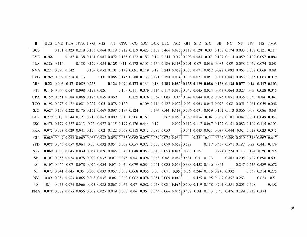
Figure 6. DAPC scatter plots by sites and inferred clusters, and box plots from Mexican (A) and

Central American ORs. ..................................................................................................... 48

Figure 7. Diagrams of relative migration between NWCR sites, behaviors, and DAPC clusters 49

Figure 8. Diagrams of relative migration between ETP sites ....................................................... 50

Figure 9. Diagrams of relative migration between ETP clusters .................................................. 51

Figure 10. Unrooted neighbor-joining trees of NWCR individuals ............................................. 52

Figure 11. Unrooted neighbor-joining trees of NWCR sampling sites and behaviors ................. 54

Figure 12. Unrooted neighbor-joining tree of ETP individuals constructed using Da ................. 55

Figure 13. Unrooted neighbor-joining tree of ETP sampling sites ............................................... 56

Figure 14. Unrooted neighbor-joining tree of ETP DAPC clusters. ............................................. 57

9

ABSTRACT

Author: Silver-Gorges, Ian, M. MS Institution: Purdue University Degree Received: May 2019 Title: Evidence for Hierarchical Structuring and Large-Scale Connectivity in Eastern Pacific

Olive Ridley Sea Turtles (Lepidochelys Olivacea) Committee Chair: Frank Paladino

Inferring genetic population structure in endangered, highly migratory species such as sea

turtles is a necessary but difficult task in order to design conservation and management plans.

Genetically discrete populations are not obvious in highly migratory species, yet require unique

conservation planning due to unique spatial and behavioral life-history characteristics.

Population structure may be inferred using slowly evolving mitochondrial DNA (mtDNA), but

some populations may have diverged recently and are difficult to detect using mtDNA. In these

cases, rapidly evolving nuclear microsatellites may better elucidate population structuring.

Bayesian inference and ordination may be useful for assigning individuals to inferred

populations when populations are unknown. It is important to carefully examine population

inference results to detect hierarchical population structuring, and to use multiple,

mathematically diverse methods when inferring and describing population structure from genetic

data.

Here I use Bayesian inference, ordination, and multiple genetic analyses to investigate

population structure in Olive ridley sea turtles (ORs; Lepidochelys olivacea) nesting in

northwestern Costa Rica (NWCR) and across the entire Eastern Tropical Pacific (ETP).

Mitochondrial DNA did not show structure within NWCR, and existing data from prior studies

are not appropriately published to compare NWCR to Mexican ORs. In NWCR, Bayesian

inference suggested one population, but ordination suggested four moderately structured

populations with high internal relatedness, and moderate to high levels of connectivity. In the

ETP, Bayesian inference suggested a Mexican and Central American population, but hierarchical

analysis revealed a third subpopulation within Mexico. Ordination revealed nine cryptic clusters

across the ETP that primarily corresponded to Mexican and Central American populations but

contained individuals from both populations, some from other, distant nesting sites. The

subpopulation within Mexico was well-defined after ordination, and all clusters displayed high

10

internal relatedness and moderate genetic differentiation. Bottlenecks were detected in both

putative populations, at seven Mexican and two Central American nesting beaches, and in six out

of nine inferred clusters, including three out of four Mexican clusters. Bottleneck events may

have played some role in cluster differentiation. Migration was significant from Mexico to

Central America at multiple levels, but did not necessarily agree with potential migrants

elucidated by ordination. Migration was generally lower between ordination-inferred clusters

than between nesting sites or Bayesian-inferred clusters. Phylogenetic trees generally supported

structuring by ordination, rather than by Bayesian inference. Structuring in ordination not tied to

bottleneck events could be due to mating behaviors or patterns of nesting beach colonization

dictated by environmental features.

In this study, ordination provided a more practical and nuanced framework for defining

MUs and DIPs in ETP ORs than did STRUCTURE. This may be due to hierarchical structuring

within ETP ORs that may be present in other sea turtle populations and species. In the case of

ETP ORs, hierarchical structure may be an artefact of recent population bottlenecks and

subsequent recolonization of nesting beaches, or due to mating at foraging grounds or along

migratory routes. Bayesian inference may not be the best method for population inference in

highly migratory species such as sea turtles, which have a high potential for broad scale genetic

connectivity, and therefore may display hierarchical population structuring not easily related to

nesting sites. Future studies, and perhaps published studies, should incorporate Bayesian

inference and ordination, as well as other measures of population divergence and descriptive

statistics, when searching for population structure in highly migratory species such as sea turtles.

11

INTRODUCTION

Sea Turtle Population Biology

Understanding the population genetics of endangered species is critical to identifying

where and how many distinguishable populations there may be in a region, and can aid in

developing conservation plans for those populations. For sea turtle conservation this is often

done by designating Management Units (MUs), which are genetically discrete groupings of

nesting assemblages (Komoroske et al. 2017). Nesting assemblages are obvious choices for

defining turtle populations, as females are easily accessible for sampling as they come ashore to

nest, and typically display natal homing (Lohmann et al. 2008, Lohmann et al. 2017). Defining

MUs is a critical step towards effective sea turtle conservation and is continually highlighted as a

priority for global sea turtle research (Hamann et al. 2010, Rees et al. 2016).

Six out of the seven species of sea turtles are listed as threatened or endangered by the

International Union for the Conservation of Nature (IUCN; IUCN 2018). These species are

distributed globally, and have faced intense pressure from habitat loss due to anthropogenic

development and abiotic alteration as a result of climate change. Populations are also impacted

by indirect and direct take from fisheries operations, as well as by legal and illegal poaching of

eggs and adult turtles for consumption and decorative products (Valverde et al. 2012, Foran and

Ray 2016). In addition, sea turtles undertake extensive developmental and seasonal migrations

between breeding and foraging grounds (Plotkin 2003, Broderick et al. 2007, Shillinger et al.

2008) that expose them to additional risk factors. For example, these migrations may put turtles

at risk of higher annual mortality due to spatial overlap with anthropogenic activities (Hart et al.

2014, Vander Zanden et al. 2016). Increased exposure to risk factors complicates efforts to

define MUs, as genetically related turtles may be found at opposite ends of an ocean basin

(Bowen et al. 1997). Sea turtles in different locations require unique management plans, but

genetically related, regionally-defined populations (such as ontogenetically discrete assemblages,

related breeding or foraging assemblages, as well as distant but genetically similar nesting

assemblages) necessitate management plans to account for this genetic connectivity.

12

Sea Turtle Population Genetics

Mitochondrial DNA

Genetic analyses of mitochondrial DNA (mtDNA) and highly polymorphic regions in

nuclear DNA (nDNA) have allowed researchers to designate more informative MUs that capture

much of the genetic variation within a species regionally and globally (Bowen et al. 2007,

Komoroske et al. 2017). Research focusing on the D-loop of mtDNA has been integral towards

this end (Bowen et al. 2007). Sequences (haplotypes) from the D-loop of mtDNA diverge on a

scale of tens of thousands to millions of years in Testudines (Avise et al. 1992). Sea turtles

typically share mtDNA D-loop haplotypes within regions (such as isolated islands or the

northern and southern areas of an ocean basin; Bowen et al. 2007). Previously, studies utilized

~400 basepair (bp) mtDNA D-loop sequences to characterize sea turtle populations until 2006,

when oligonucleotide primers were reported that allowed for the amplification of ~800bp

sequences (Abreu-Grobois et al. 2006). While the ~400bp sequences capture many of the

variable sites within the D-loop, the ~800bp sequences overlap the ~400bp sequences and help to

further refine the relationships between populations. Haplotype sequences are made publicly

available on Genbank (www.ncbi.nlm.nih.gov/genbank/) at the time of publication, allowing

researchers to compare haplotypes between populations to determine population structure.

mtDNA D-loop haplotypes (based on both the ~400bp and ~800bp sequences) and haplotype

frequencies have been used extensively to delineate MUs in most sea turtle species (Bowen et al.

2007).

Nuclear DNA

Codominant, repetitive, hypervariable markers in nDNA termed microsatellites, have also

been used to characterize population structure in sea turtles. Microsatellites are more likely to

vary between individuals than are D-loop sequences, but certain alleles may be conserved within

reproductively isolated MUs (Komorske et al. 2017). Additionally, microsatellite alleles are

passed down by both males and females to offspring in diploid species. Thus, an informative

panel of microsatellites may capture divergences that are too recent to be represented by D-loop

sequences or that are occurring in near-panmictic populations (i.e. Rodriguez-Zarate et al. 2018)

amd illustrate male-mediated gene-flow (i.e. FitzSimmons et al. 1997, Roberts et al. 2004).

13

nDNA can also used to conduct bottleneck, migration, and kinship analyses to better understand

the factors influencing the formation of MUs (see Blouin et al. 2003, Putman and Carbone 2014

for reviews of these analyses). However, microsatellite allele lengths (in bps; the metric

measured to genotype individuals) are sensitive to polymerase chain reaction (PCR)

temperatures and variation in electrophoresis conditions, making it difficult to directly compare

among studies.

Genetic Analyses in Population Biology

F and F-like Statistics and Analysis of Molecular Variance

mtDNA sequences and nDNA genotypes may be subjected to mathematical equations

and models to characterize and understand population structure. These analyses ultimately can be

used to define MUs. F-statistics and F-like statistics (Fst and Fis, 𝚯𝚯st, D; Wright 1949, Weir and

Cockerham 1984, Jost 2008, respectively) and Analysis of Molecular Variance (AMOVA;

Excoffier et al. 1992) are commonly used to identify MUs with significantly different haplotype

and allele frequencies. These metrics can also provide a quantitative measure of the strength of

population structuring (Fst) and even inbreeding (Fis).

Bottleneck Analysis

It is also possible to investigate evolutionary processes that form MUs. For example,

population bottlenecks may occur when populations are reduced dramatically in size. Globally,

many sea turtle populations have experienced bottlenecks after reaching historic minima in the

mid-20th century (see Jensen et al. 2013A and references therein). Populations now recovering

from bottleneck events are expected to have relatively low genetic diversity (Bouzat 2010 and

references therein), which may have consequences for population resilience (Keller et al. 1994,

Frankham et al. 1999, Eldridge et al. 1999). The genetic signatures left by bottleneck events may

be identified using metrics and likelihood functions that analyze mtDNA (D; Tajima 1989) and

nDNA (M-ratio: Garza and Williamson 2001; BOTTLENECK: Piry et al. 1999, Cornuet and

Luikart, 1996). However, methods for detecting bottlenecks using nDNA data have come under

criticism for their sensitivity to the fit of the data to specific mutational models and for their

sensitivity to specific input parameters (Cornuet and Luikart 1996, Leblois et al. 2006, Peery et

14

al. 2012). Despite this, such metrics may be useful for understanding population structure if

properly calculated and interpreted (Putman and Carbone 2014). Geographically discrete

bottleneck signatures, such as those present at only some nesting sites within an ocean basin,

may identify recent and ongoing take of turtles (i.e. fisheries bycatch, poaching of eggs and

adults on beaches) that can be addressed in policy and management plans.

Relatedness Analysis

Relatedness (r) may also be informative towards population structure (Blouin 2003).

Relatedness is measured on a scale from 0 to 1 for any two individuals based on how much of

their genome is shared (0 being none, 1 being all). In a diploid family, meiosis occurs between

each “generation link” (L), and the probability of a copy of a gene being passed on from one

individual to another is 0.5 (Davies et al. 2012). The relatedness coefficient between any two

individuals is then the sum of the probability of a gene being passed down for all of the links

between the two individuals, or

r=∑p(0.5)L

where p is the number of paths between two individuals and L is each link between two

individuals within one path. For example, a parent has a 50% chance of passing a copy of any

gene to its offspring. r for parent-offspring (po) relationships is:

rpo=0.51= 0.5

There is only one path between the two individuals, and there is only one link. If that offspring

has a full sibling, there are two links between the siblings (offspring to parent, parent to sibling),

and two paths connecting the siblings (one through each parent). Therefore:

rsib=0.52+0.52= 0.5

In practice, estimating relatedness coefficients from genotypic data is not based on categorical

relationships between individuals, but on the percentage of the genome (based on shared alleles)

that is identical by descent. Lynch and Ritland (1999) and Queller and Goodnight (1989)

developed algorithms to estimate relatedness between individuals based on genotypes and allele

frequencies. While these estimators are sensitive to the number of loci used and the number of

sampled related individuals, and are not always in complete agreement (Wang 2002, Blouin

2003), on a population scale they may provide a sense of structuring and can complement F-

statistics (Queller and Goodnight 1989).

15

Sea turtles are known to display natal homing during breeding seasons (Lohmann et al.

2017) and therefore turtles at one nesting beach, or within a certain nesting area, may be more

related to each other than to turtles that nest further away. However, relatedness patterns may

also be influenced by mating behavior at nesting aggregations (such as arribadas) or by mating

away from nesting beaches (i.e. at foraging grounds). Related groups of turtles are expected

within nesting assemblages, but related groups that do not share nesting beaches may suggest

that other areas are used for mating, such as foraging grounds and migratory routes. These areas

would gain importance as areas to protect to maintain the genetic diversity within and between

MUs. Related groups that do not correspond to nesting regions may also suggest that other

environmental or endogenous factors are affecting dispersal from and recruitment to nesting

assemblages.

Migration Analysis

Migration, or the transition of individuals from one population to another geographically

separate population, may also shape and affect population structure (Putman and Carbone 2014,

Sundqvist et al. 2016 and references therein). Migration may erode population structure if

individuals consistently move between populations, and may even lead to misleading estimates

of population differentiation (Dias 1996). This is particularly true for asymmetric migration, in

which individuals move more frequently from some populations to other populations, rather than

evenly between populations. In some cases, asymmetric migration may produce misleading

signatures of population differentiation (i.e. Whitlock and Mcauley, 1996) that can lead to

misdirected management efforts if not properly identified (Dias 1996, Pringle et al. 2011).

Software and metrics that estimate migration based on genetic data are often subject to

internal assumptions of loci being in linkage equilibrium or low levels of migration between

populations with high levels of differentiation (i.e. BayesAss; Wilson and Rannala 2003, Faubet

et al. 2007). Some analyses only measure migration within one generation (i.e. GeneClass; Piry

et al. 2004), and/or assume symmetric migration (i.e. Gst: Nei 1973; G’st: Hedrick 2005, and D:

Jost 2008). Such analyses may not be appropriate for species such as sea turtles, which are

already highly migratory (in a spatial sense of the term) and long lived (and therefore are likely

to have overlapping generations). Further, asymmetric migration is known in marine species with

environmentally driven dispersal of neonates and juveniles (Siegel et al. 2003, Cowen and

16

Sponaugle 2009). For example, sea turtles display current driven dispersal as hatchlings (Hays et

al. 2010), and adult movements may even be constrained or influenced by environmental

features (i.e. Rodriguez-Zarate et al. 2018). Analyzing asymmetric migration (i.e. in divMigrate;

Sundqvist et al. 2016) is not a well-tested practice. While this analysis may be inaccurate with

high levels of migration (Sundqvist et al. 2016), it should prove useful to understanding sea turtle

population structure and designating effective MUs.

Genetic Distance Analysis

Identifying the factors that lead to the formation of MUs may further validate putative

MUs, and provide valuable information towards conservation of MUs. However, MUs must be

identified before population structure may be characterized and investigated. Identifying MUs

ad-hoc is not always straight-forward. For sea turtles, one MU may span multiple nesting

beaches and show connectivity to distant foraging grounds. Differences between nesting turtles

from different ocean basins may be empirically hypothesized and tested, but it is not so simple to

identify genetic boundaries when looking within a region (such as an ocean basin). Constructing

exploratory phylogenetic trees of individuals or sampling sites may provide a basis for MU

designation, but are sensitive to the tree-building method used and require prior designation of

sub-populations (Putman and Carbone 2014).

Population Inference

Bayesian Inference

STRUCTURE (Pritchard et al. 2000) is a canonical program for investigating population

structure. STRUCTURE uses Bayesian inference to identify the most likely partitions in genetic

data sets (K), but is processing-heavy and subject to assumptions of Hardy-Weinberg equilibrium

that may reduce the informative power of a data set (Putman and Carbone 2014). Hierarchical

analyses are often necessary to elucidate the true population structure, as sub-structuring may be

obscured by broader structuring (Kalinowksi 2011, Putman and Carbone 2014). STRUCTURE

has been shown to incorrectly identify K based on its internal ad-hoc likelihood estimator

(Pritchard et al. 2000, Evanno et al. 2005), and is subject to sampling bias when populations are

not evenly samples (Peuchmaille 2016). STRUCTURE may also be inherently biased towards

17

K=2 (Janes et al. 2017). These limitations can be ameliorated to an extent using post-processing

algorithms such as those included in Structure Harvester (Earl 2012), but these programs still

rely on the STRUCTURE output to determine the most likely number of genetic groupings.

Ordination

Thus, it is important to compare results from multiple different clustering algorithms.

Ordination of genetic data, in which individuals are plotted as points on a 2-dimensional plane,

does not rely upon the same assumptions as Bayesian algorithms nor does it require as much

processing power. Common ordination methods include Principal Component Analysis (PCA; in

which axes are constructed to maximize variance among data) and Principal Coordinate Analysis

(PCoA; in which the data are projected onto a coordinate plane to maximize dissimilarities

between points). However, PCA assumes that variance among points will be homogenous, which

is not often true for genetic data sets, and PCoA requires the correct specification of a mutational

model to accurately infer true differences between points, which is difficult with datasets that do

not conform nicely to any common mutational models (Jombart et al. 2009, Odong et al. 2013,

Putman and Carbone 2014).

The R package adegenet (Jombart 2008, Jombart and Ahmed 2011) implements a method

termed Discriminant Analysis of Principal Components (DAPC, Jombart et al. 2010) which plots

individuals in a coordinate plane based on genotypic data, uses a k-means algorithm to identify

the most likely K, and then calculates axes to maximize distance between clusters and minimize

variance within clusters. DAPC may outperform STRUCTURE when hierarchical structuring is

present in a dataset (Jombart et al. 2010), however the limitations of DAPC and ordination in

general are not well known (Putman and Carbone 2014). Selecting the number of axes retained

to plot individuals and the most likely K are left up to the user and may therefore introduce bias

into an analysis (Putman and Carbone 2014). Despite the disadvantages and differences of these

exploratory methods, comparing their results on a single dataset can increase confidence in

identifying true population structure present within a dataset, and can ultimately lead to more

effective MU designations.

18

Olive Ridley Sea Turtles

Global Population Biology

MUs are not well defined for Olive ridley (OR) sea turtles (Lepidochelys olivacea). ORs

are the most abundant sea turtle and are not listed as endangered (Abreu-Grobois & Plotkin

2012). However they are subject to illegal and legal take of eggs (Valverde et al. 2012), and

constitute a large proportion of fishers bycatch (Moore et al. 2009). Researchers have

documented decades-long declines in the number of individuals participating in mass nesting

events termed “arribadas” (Fonseca et al. 2009). Despite this, OR population structure has not

been comprehensively studied and MUs remain largely undefined.

ORs may be divided into broad, genetically distinct regional populations based on

mtDNA in the Atlantic Ocean (ATL; Bowen et al. 1997, Plot et al. 2012), the Indo-Pacific region

(IP; Bowen et al. 1997, Jensen et al. 2013B, Bahri et al. 2018), India and Sri Lanka (IND; Bowen

et al. 1997, Shanker et al. 2004B), and the Eastern Tropical Pacific Ocean (ETP; Bowen et al.

1997, Lopez-Castro & Rocha-Olivares 2005, Cortes et al. 2015). The ATL population of Olive

ridleys is the smallest (Bowen et al. 1997, Plot et al. 2012). Only turtles nesting at Guinea Bissau

have been systematically sampled and had mtDNA haplotypes sequenced at ~800bps (Plot et al.

2012). The IP population does not host any arribada beaches but is widespread across northern

Australia, the southeast Asian island, and the Asian and continent (Bowen et al. 1997, Jensen et

al. 2013B, Bahri et al. 2018). Several ~800bp mtDNA sequences are available from Indonesia,

Papua New Guinea, and Australia, but only Australian Olive ridleys have been studied with an

intent towards designating MUs (Jensen et al. 2013B). The IND population is large and has faced

intense anthropogenic pressure (Shanker et al. 2004A). Haplotypes from this region share a 7bp

deletion with Kemps ridley sea turtles (Lepidochelys kempii) and are thought to be basal for the

species (Bowen et al. 1997, Shanker et al. 2004B). However, mtDNA sequences are only

available at ~400bps from this population.

Eastern Pacific Population Biology

The ETP population is robust, with multiple arribada nesting sites and high-density

solitary nesting sites, but seemingly minimal structuring among continental sites (Lopez-Castro

and Rocha-Olivares 2005, Valverde et al. 2012). In accordance with this, phylogeographic

19

studies of ORs have suggested that the EP population is no more than 250,000-300,000 years old

(Bowen et al. 1997, Jensen et al. 2013B). Analyses of mtDNA and nDNA data suggest that

Olive ridleys nesting on the Baja Peninsula (Mexico) may comprise a discrete MU (Lopez-

Castro & Rocha-Olivares 2005, Rodriguez-Zarate et al. 2013). nDNA has shown that arribada

and non-arribada ORs in Costa Rica do not comprise discrete populations (Jensen et al. 2006,

Koval 2015). Koval (2015) analyzed microsatellite data from solitary and arribada ORs nesting

at three sites in Northwestern Costa Rica (NWCR; Playa Grande, Playa Ostional, and Playa

Nancite) using STRUCTURE and DAPC. STRUCTURE suggested all nesting sites and

behaviors comprised one population (in accordance with Jensen et al. 2006), but DAPC

identified 4 clusters comprising individuals from all nesting sites and both behaviors with

moderate overall structure (Fst=0.103; Koval 2015). There was no evidence of a bottleneck

event overall, within sampling sites, or within DAPC clusters (Koval 2015).

While mtDNA and nDNA data do not show obvious population structure among

continental ETP nesting sites at fine scales, nDNA suggest a north-south population split across

the entire ETP when analyzed in STRUCTURE (Rodriguez-Zarate et al. 2018). However, it is

difficult to test for this split using mtDNA as haplotypes are not well-reported from Central

America. Further, while Rodriguez-Zarate et al. (2018) found that environmental variables

(namely oceanographic features) play a role in this structuring, the authors did not report

hierarchical or comparative analyses for population structuring. They suggest two panmictic

populations of ETP ORs, one comprising Mexican turtles and the other comprising Central

American turtles.

Study Questions

In light of the recently uncovered north-south population split in ETP Olive ridleys

(Rodriguez-Zarate et al. 2018), as well as the lack of a robust mtDNA data set from Central

America, I sought to answer four questions in this study:

1) Would analysis of mtDNA sequence data support or refine population structure in

NWCR or ETP ORs?

2) Would analysis of ETP OR nDNA elucidate substructuring within Mexican and

Central American populations?

20

3) Would ordination (DAPC, as implemented in adegenet) produce cryptic clusters in

both NWCR and ETP ORs?

4) What processes might be contributing to the formation of inferred populations, and

which inferred populations were best supported by multiple analyses (genetic distances trees,

bottleneck analysis, relatedness analysis, and migration analysis)?

21

METHODS

NWCR mtDNA Analysis

Blood samples and skin samples from 118 Olive ridley turtles collected in 1999 (Playa

Nancite, n=7; Clusella-Trullas et al. 2006), and in 2011-2012 and 2013-2014 (Playa Ostional

n=78; Playa Grande, n=33) were processed at Purdue University Fort Wayne in 2014 (Koval

2015). DNA was extracted from samples using QIAGEN DNeasy Blood and Tissue Kits

following the manufacturer’s protocol and frozen at -20 ºC. Samples were diluted to 25 ng μl-1

before PCR.

~800 bp sequences from the D-loop of the mtDNA control region were amplified for 60

turtles from Playas Nancite, Ostional, and Grande using primers LTEi9 (5’-

AGCGAATAATCAAAAGAGAAGG-3’) and H950 (5’-GTCTCGGATTTAGGGGTTTA-3’;

Abreu-Grobois et al. 2006, Jensen et al. 2013B). PCR reactions were conducted using QIAGEN

Taq PCR Master Mix Kits following the manufacturer’s protocol. I used an incubation profile

previously described by Jensen et al. (2013B): denaturing at 94°C for 5 minutes, then 35 cycles

of 45 seconds at 94°C, 45 seconds at 52°C, and 45 seconds at 72°C, and final extension at 72°C

for 5 minutes. PCR products were run on agarose gels to ascertain quality and product size.

PCR products measured to ~800 bps were purified using ExoSAP-It (Thermo) and sent to

Genewiz (New Jersey, USA) for Sanger sequencing. Forward and reverse sequences were

trimmed to ~400bps and ~800bps, assembled, and aligned in Geneious v.11 (Kearse et al. 2012)

using the CLUSTALW algorithm (Thompson et al. 2003). ~400bp and ~800bp Olive ridley

mtDNA sequences from prior studies (Bowen et al. 1997, Shanker et al. 2004B, Lopez-Castro &

Rocha-Olivares 2005, Plot et al. 2012, Jensen et al. 2013B, Revuelta et al. 2015,Beltran et al.

2016, Bahri et al. 2018) were procured from Genbank and aligned with sequences from this

study. New and existing haplotypes from NWCR were determined using DnaSP 6 (Rozas et al.

2017). All haplotypes were named as per National Marine Fisheries Services protocols (Peter

Dutton, personal communication). New sequences (n=4) were re-sequenced for confirmation and

deposited in Genbank (Accession #s MK749418, MK749419, MK749420, MK749421).

Haplotype networks were generated for sequences from this study in TCS (Clement et al. 2000)

and modified for publication using tcsBU (Murias dos Santos et al. 2015). Genetic diversity at all

22

sites was quantified by calculating mean Haplotype Diversity (H) and mean Nucleotide Diversity

(π) in Arlequin v.3.5 (Excoffier & Lischer 2010).

Microsatellite Amplification

Amplification and characterization of microsatellite loci from ORs in NWCR (Koval

2015) and the ETP; Rodriguez-Zarate et al. 2018) are described in the original studies,

respectively. NWCR data were obtained from the author (Julianne Koval, personal

communication), and ETP OR data were obtained from https://doi.org/10.5061/dryad.nj344m5

(Rodriguez-Zarate et al. 2018). Data from Koval (2015) will be referred to as NWCR, and data

from Rodriguez-Zarate et al. (2018) will be referred to as ETP. Abbreviations of ETP sampling

sites used here may be found in the supplemental data for Rodriguez-Zarate et al. (2018).

Analyses

F and F-like Statistics and Analysis of Molecular Variance

Pairwise and overall Fst (Wright 1949) and Φst (an Fst estimator for mtDNA), single site

Fis (Wright 1949), pairwise θst (Weir & Cockerham 1984), Jost’s D (Jost 2008), and Analysis of

Molecular Variance (AMOVA; Excoffier et al. 1992) were quantified in Arlequin v. 3.5

(Excoffier and Lischer 2010) and GenAlex (Peakall and Smouse 2006) for mtDNA and nDNA

(when applicable) from NWCR ORs. Alpha levels for pairwise Fst and D were adjusted using a

Bonferroni correction for multiple tests. Fst, or Wright’s Fixation Index, compares haplotype or

allele frequencies between putative populations relative to the overall sample and produces a

measurement of population differentiation between 0 and 1 (0 being no difference between

populations; 1 being total difference between populations). Fis (Wright 1949) is similar to Fst,

and measures the amount of genetic variation contained within individuals within

subpopulations. Θst, or Weir and Cockerham’s (1984) Fst, is an estimator of Wright’s Fst for

mtDNA data that takes the number of haplotypes and sample size into account. D (Jost 2008)

measures the fraction of allelic variation among populations and is thought to be more

appropriate for analyzing microsatellite data than Fst (Putman and Carbone 2014). AMOVA is

similar to conventional ANOVAs, but uses the sum of square molecular distances between

haplotypes or alleles within and between populations to assess population differentiation.

23

Population Inference

STRUCTURE (Pritchard et al. 2000) and adegenet (Jombart et al. 2008) were used to

assign individuals to putative MUs (K) based on microsatellite genotypes. K represents the

number of inferred genetically discrete populations; whether each inferred population represents

an MU is explored in the discussion. Initial STRUCTURE parameters and results are reported in

Koval (2015; NWCR) and Rodriguez-Zarate et al. (2018; ETP). I analyzed Mexican and Central

American population identified by Rodriguez-Zarate et al. (2018) for internal structuring.

STRUCTURE was run 10 times for each K=1-15, with a burn-in of 50,000 generations and an

MCMC of 100,000 generations for Mexican and Central American populations. Each run

assumed correlated allele frequencies (Falush et al. 2003) and historical admixture between

populations (Pritchard et al. 2000). Runs were repeated with and without sampling location as a

prior (LOCPRIOR; Hubisz et al. 2009). STRUCTURE was run hierarchically until the most

likely K=1 (see below).

STRUCTURE output files were analyzed in STRUCTURE HARVESTER v.0.6.92 (Earl

2012) to determine the true number of K using multiple metrics. The estimated log probability of

data pr(X|K) given a particular value of K allows the estimation of the most likely number of

clusters (Pritchard et al. 2000). The ad hoc delta-K method (Evanno et al. 2005) reports the

second-order rate of change of the log probability of data regarding the number of clusters,

which typically peaks at the appropriate value of K. The admixture model calculates the

fractional probability (Q) of individuals belonging to each population.

A Discriminant Analysis of Principal Components (DAPC; Jombart et al. 2010) was run

for both data sets using adegenet (Jombart et al. 2008) as implemented in R. Genotype data were

transformed into a coordinate format for Principal Coordinate Analysis (PCA). The most likely

number of clusters was determined using k-means clustering and a Bayesian Information

Criterion (BIC), and all principal components (PCs) were retained. A Discriminant Analysis

(DA) was run on the PCA to maximize separation between groups. As suggested by Jombart et

al. (2010), 100% of the initial PCs were retained when identifying K, ~80% of PCs were retained

during discriminant analysis, and the first n≤10 axes of the discriminant analysis were retained.

DAPC was also run by sampling site for both data sets to examine geographic population

structuring. Each DAPC was cross-validated and re-run with suggested PCs to minimize error

(Jombart et al. 2010).

24

STRUCTURE and adegenet K assignments were tested for population structure (Fst and

Fis within AMOVA in Arlequin; Pairwise Fst and D in GenAlex), genetic distances in

Neighbor-Joining trees (Saitou and Nei 1987), bottleneck signatures (BOTTLENECK; Cornuet

and Luikart 1996, Piry et al. 1999), relatedness (LRM: Lynch and Ritland 1999; and QGM:

Queller and Goodnight 1986, in GenAlex), and differential migration (divMigrate, Sundqvist et

al. 2016). Fst, AMOVA, and D were calculated over 10,000 bootstrap replicates.

Genetic Distance Analysis

Neighbor-joining (NJ; Saitou and Nei 1987) distance trees were constructed for all

individuals, sampling sites, and DAPC clusters using Nei et al.’s (1983) Da with 1000 bootstrap

replicates as implemented in the program Populations 1.2.30

(http://bioinformatics.org/populations/; Olivier Langella, 1999). NJ trees are constructed by

pairing the least genetically distant individuals or units at the tips of the tree, and working

backwards to build the branches and base of the tree (Saitou and Nei 1983). Populations offers

many options for calculating distances between individuals and populations, each of which vary

slightly (see http://bioinformatics.org/populations/). I chose Da (Nei et al. 1983) as a distance

measure in part because of a potential bug in Populations that prevented the completion of trees

based on other distance measures, and in part because Da is thought to produce more accurate

topologies than other distance measures (see Nei et al. 1983). NJ trees are not as robust as

maximum likelihood or Bayesian methods for inferring ancestral (i.e. population of origin)

relationships between individuals and populations (Putman and Carbone, 2014), but may prove

useful as an exploratory method for further assessing and comparing population structuring

inferred by other methods.

Bottleneck Analysis

Bottleneck analysis was conducted for sampling sites and all inferred populations (via

STRUCTURE and DAPC) in BOTTLENECK (Piry et al. 1999). BOTTLENECK was run for

10,000 iterations of the two-phase mutation model (TPM; DiRienzo et al. 1994) as suggested for

microsatellite data by Piry (1999; 95% Stepwise Mutation Model [SMM; Ohta and Kimura

1973] in the TPM with a variance of 12). BOTTLENECK was also run with TPM settings

suggested by Piry et al. in web documentation for the program

25

(http://www1.montpellier.inra.fr/CBGP/software/Bottleneck/pub.html; 0% SMM in the TPM and

36 variance). In the SMM, microsatellites are only modeled to mutate by one repeat length per

mutational event, while in the TPM they may mutate by one or more repeats per mutational

event. The TPM is thought to be more representative of actual processes of mutation and

evolution than the SMM (DiRienzo et al. 1994, Piry et al. 1999). The TPM is generally more

conservative than the SMM in inferring bottleneck events, as alleles that differ by more than one

repeat still have a probability of coming from one mutational event, rather than multiple

mutational events (Sainudiin et al. 2004).

Relatedness Analysis

Pairwise relatedness values between individuals were calculated over 10000 iterations

using estimators designed by Ritland and Lynch (1999) and Queller and Goodnight (1989) as

implemented in GenAlex (Peakall and Smouse 2006). Mean pairwise relatedness was then

examined relative to overall relatedness for sampling sites and all inferred populations (via

STRUCTURE and DAPC). Queller and Goodnight’s (QGM; 1989) estimator is a coefficient

based only on estimated identity by descent (IBD; Grafen 1985). Ritland and Lynch’s (LRM;

1999) estimator uses a regression calculation to determine relatedness coefficients for any pair of

individuals based on shared IBD alleles, but can perform poorly if few related individuals are

sampled, or if loci are too highly polymorphic (Blouin 2003). Both estimators may also have

high variances when few loci (n<20) are used, but, as mentioned above, can provide a good

estimation of relatedness between groups of individuals (Queller and Goodnight 1989, Blouin

2003).

Migration Analysis

divMigrate (Sundqvist et al. 2016) was used to calculate differential migration between

all sampling sites, STRUCTURE clusters, and DAPC clusters from both data sets. divMigrate

estimates directional migration based on one of three population metrics specified by the user:

Nm (Alcala et al. 2014), Gst (Hedrick and Goodnight 2005) and D (Jost 2008). In idealized

asymmetric migration from one population (A) to another (B), population B is expected to share

alleles with population A in the same proportions (albeit lower frequencies) as they exist in

population A, and may also contain alleles not found in population A.

26

divMigrate uses the genetic distance measures mentioned above and allele frequencies to

calculate scaled, relative migration between two populations on a 0 to 1 scale based on this

theory of the genetic signature of migration. divMigrate is known to incorrectly identify

migration at high levels of migration and low (n<~50) sample sizes (Sundqvist et al. 2016), and

each estimator performs differently. Gst is thought to perform best at accurately identifying

differential migration relative to Nm and D (Sundqvist et al. 2016), but I chose to run divMigrate

with all three parameters for 1000 bootstrap replicates each to avoid biases from any individual

estimator.

27

RESULTS

Mitochondrial DNA Analysis

I observed ten ~800bp haplotypes from 60 turtles nesting at Playa Nancite (n=7), Playa

Grande (n=17), and Playa Ostional (n=36; Table 1; Figures 1&2). Haplotypes are named

sequentially as per National Marine Fisheries Service conventions (Peter Dutton, personal

communication). Overall haplotype diversity (H=0.5657±0.0783 SD) and nucleotide diversity

(π=0.0014±0.0012 SD) were comparable to those reported in other studies of Pacific Olive

ridleys (i.e. Jensen et al. 2013B, Lopez-Castro & Rocha-Olivares 2005) and did not vary between

sites (as suggested by overlapping standard deviations; Table 1).

There was no evidence that any of the three sites were genetically distinct from each

other as determined by pairwise Φst (Φst = -0.05 ± 0.00021, p = 0.37 - 0.79), pairwise θst (θst = -

0.03 ± 0.02, p = 0.61 - 0.79), and AMOVA (Fst=-0.02, p=0.65). I attempted to compare

haplotype frequencies from this study to those reported from previous studies on EP Olive ridley

mtDNA sequences (i.e. Lopez-Castro & Rocha-Olivares 2005) but were unable to accomplish

this analysis due to the lack of a consistent, systematic nomenclature for Olive ridley haplotypes

(Peter Dutton, personal communication). However, Lo46 comprised 68% of the haplotypes I

found, which is consistent with (albeit lower than) Lopez-Castro and Rocha-Olivares’ (2005)

findings from Mexican Olive ridleys (~90%) and suggests a lack of population differentiation

between Mexican nesting assemblages and these Costa Rican nesting assemblages.

Summary of Nuclear DNA Results from Previous Studies

Summary and descriptive statistics for microsatellite data from NWCR and the ETP, as

well as initial STRUCTURE and DAPC results, are reported in the original studies: Koval

(2015) and Rodriguez-Zarate et al. (2018). Briefly, Koval (2015) found that K=1 in NWCR ORs,

and Rodriguez-Zarate et al. (2018) found that K=2 in ETP ORs, with a division between

Mexican and Central American ORs (AMOVA; Fct=0.028). Koval (2015) also conducted DAPC

and found 4 clusters with moderate differentiation (Fst=0.103) that each contained arribada and

solitary nesting individuals from all three sampling sites. Koval (2015) did not find evidence for

28

bottleneck events. Pairwise Fst, pairwise D, and AMOVA are reported for ETP ORs in

Rodriguez-Zarate et al. (2018).

Population Inference in ETP ORs

Hierarchical analysis in STRUCTURE with location as a prior (locprior) weakly

suggested a putative subpopulation in Mexico consisting primarily of turtles nesting at PAR

(Figure 3A). AMOVA and pairwise Fst confirmed significant, yet moderate structuring between

PAR and other Mexican sites (AMOVA: Fst=0.067, p<0.001; Pairwise Fst: Fst=0.066,

p<0.001). Hierarchical analysis of STRUCTURE in Mexico without locprior, as well as in

Central America with and without locprior were unable to discern obvious structure (Figure 3A,

B). DAPC by nesting site confirmed STRUCTURE results: Mexican and Central American

nesting beaches split along the first axis, PAR separated from other Mexican nesting beaches,

and the Central American nesting beaches showed admixture (Figure 4). However, assignment

proportions were not high (mean=65.3±0.002SE; Figure 4).

DAPC by inferred clusters produced similar results to the same analysis run on NWCR

ORs. DAPC elucidated 9 discrete clusters with high assignment proportions (mean=0.99+-

0.003SE; Figure 4). Clusters largely aligned with Mexican and Central American populations,

but contained individuals from multiple nesting sites, some as distant as ~3500km as the crow

flies (i.e. BCS and PMA) within both putative populations (Figure 4). AMOVA showed that

DAPC clusters were moderately differentiated from each other (Variance Explained=10.37%,

Fst=0.103, p<0.001; Table 2) and pairwise Fst (0.037-0.091) and D (0.111-0.507) confirmed that

all clusters were significantly different from one another (Table 3). Fis indicated significant,

moderate inbreeding in all primarily Mexican clusters (1,5,8,9) and one primarily Central

American cluster (6; Table 4).

I removed individuals assigned to one highly differentiated cluster (#8 in Figure 4) and

re-ran DAPC on the remaining individuals, which highlighted separation between the remaining

inferred clusters (Figure 5). Hierarchical discriminate analysis of Mexican and Central

American subpopulations further highlighted discrete clusters within each subpopulation that

largely corresponded to clusters in the ETP-wide DAPC (Figure 6, Table 5).

29

Genetic Distance Analysis

The NJ trees confirmed elements of STRUCTURE and DAPC analyses. I compared Nei

et al.’s (1983) Da to Latter’s (1972) Fst in a NJ tree of NWCR individuals (Figure 10), to

determine if different distance calculations would affect general tree topology. Trees constructed

with Da (Nei et al. 1983) and Fst (Latter 1972) agreed on general structuring (Figure 10) and

here I discuss trees constructed with Da. I caution that these trees are not intended to be their

own analyses of population structuring, but rather should be used to supplement analyses in

STRUCTURE and adegenet. Trees were left unrooted, as I did not intend to determine

evolutionary relationships between populations.

The NJ tree of NWCR individuals indicated weak overall structuring as indicated by near

0 bootstrap values at the base of the tree, although individuals from the same DAPC clusters,

rather than from sites or behaviors, tended to be grouped together with higher confidence

towards the tips of the tree (Figure 10). The NJ tree of CR sites indicated weak but persistent

separation between sites and behaviors as indicated by branch lengths and bootstrap values

(Figure 11). Playa Nancite was more distant from other sites and behaviors, but this should be

interpreted cautiously for reasons mentioned above. The NJ tree of DAPC clusters showed more

persistent separation than the NJ tree of sites, as indicated by higher bootstrap values at nodes

(Figure 11).

The NJ tree of ETP individuals showed weak ETP-wide structuring, but individuals

grouped into clades largely consistent with DAPC clusters with slightly higher bootstrap values

than at the base of the tree (Figure 12). The NJ tree constructed with nesting sites as populations

showed a Mexican and Central American split, and highlighted structure among Mexican sites

and the lack of structure among Central American sites (Figure 13). The NJ tree of DAPC

clusters highlighted the Mexican-Central American split, but had higher bootstrap values than

the NJ tree of nesting sites (Figure 14).

Bottleneck Analysis

BOTTLENECK results varied depending on the proportion of SMM in the TPM, and on

the test used to validate the significance of results. In general, 95% SMM inferred more

population expansion after bottleneck events than 0% SMM, which only inferred one instance of

30

heterozygosity excess (Table 5). The two-tailed Wilcoxon test conferred significance

(alpha=0.05) on heterozygosity deficiencies slightly more often than the sign test, specifically in

Central American DAPC clusters. However, both tests largely agreed on bottleneck significance,

or the lack thereof.

With no SMM in the TPM, there were no inferred bottleneck events. This may be due to

the constraints and limitations of the mutation models used in BOTTLENECK (Luikart et al.

1998, Piry et al. 1999, Putman and Carbone 2014). With 95% SMM in the TPM, both Mexico

and Central America had significant heterozygote deficiency. In Mexico, bottlenecks were

detected at 6 sites, while bottlenecks were only detected at 2 sites in Central America (Table 5).

The Wilcoxon test detected bottlenecks in 3 out of 4 Mexican DAPC clusters, and 3 out of 5

Central American DAPC clusters. However, the sign test only detected a bottleneck in cluster 8.

Relatedness Analysis

LRM and QGM showed agreement in general patterns of relatedness, but differed in

exact values of relatedness within nesting sites and putative populations. In general, LRM was

more conservative than QGM. In NWCR, relatedness was negligible overall and within nesting

sites and behaviors (Table 6). Both measures suggested that Playa Nancite displayed

significantly high relatedness relative to the entire sample, but this should be interpreted

cautiously as the sample size was low (n=7) and individuals were missing data. Relatedness was

significantly high within clusters, and ranged from 0.31-0.57 (LRM) and 0.053-0.235 (QGM).

Relatedness was higher in Mexico and Central American nesting sites, and in the two

ETP populations overall, than in NWCR sites/behaviors and overall (Tables 5 and 6).

Relatedness ranged from 0.009-0.072(LRM)/0.014-0.226(QGM) in Mexico and 0.003-

0.031(LRM)/0.022-0.097(QGM) in Central America. Relatedness was not significantly high at

PLA (QGM) and NS (both LRM and QGM). Relatedness in clusters ranged from 0.018-

0.054(LRM)/0.001-0.311(QGM). Relatedness within DAPC clusters was significantly high and

comparable to nesting sites and subpopulations in all clusters, save for #9 (QGM). Relatedness

was on average higher at nesting beaches within Mexico than across all Mexican individuals, and

vice-a-verse in Central America.

31

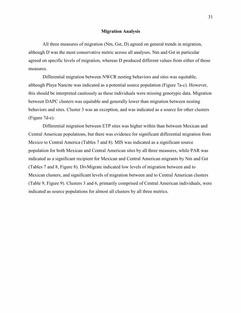
Migration Analysis

All three measures of migration (Nm, Gst, D) agreed on general trends in migration,

although D was the most conservative metric across all analyses. Nm and Gst in particular

agreed on specific levels of migration, whereas D produced different values from either of those

measures.

Differential migration between NWCR nesting behaviors and sites was equitable,

although Playa Nancite was indicated as a potential source population (Figure 7a-c). However,

this should be interpreted cautiously as these individuals were missing genotypic data. Migration

between DAPC clusters was equitable and generally lower than migration between nesting

behaviors and sites. Cluster 3 was an exception, and was indicated as a source for other clusters

(Figure 7d-e).

Differential migration between ETP sites was higher within than between Mexican and

Central American populations, but there was evidence for significant differential migration from

Mexico to Central America (Tables 7 and 8). MIS was indicated as a significant source

population for both Mexican and Central American sites by all three measures, while PAR was

indicated as a significant recipient for Mexican and Central American migrants by Nm and Gst

(Tables 7 and 8, Figure 8). DivMigrate indicated low levels of migration between and to

Mexican clusters, and significant levels of migration between and to Central American clusters

(Table 9, Figure 9). Clusters 3 and 6, primarily comprised of Central American individuals, were

indicated as source populations for almost all clusters by all three metrics.

32

Table 1. Olive ridley mtDNA control region haplotype frequencies from three nesting beaches in Costa Rica (PN: Playa Nancite; PG: Playa Grande, PO: Playa Ostional) and overall (OV) for this

study. Also shown are the number of individuals from each site (n), mean (±SD) haplotype diversity (H), and mean (±SD) nucleotide diversity (π).

Site n H (±SD) 𝜋𝜋 (±SD) Lo46 Lo73 Lo27 Lo54 Lo31 Lo52 Lo60 Lo96 Lo62 LoN11

PN 7 0.5238

(±0.2086)

0.001128

(±0.001028) 5 0 1 0 0 0 1 0 0 0

PG 17 0.5074

(±0.1403)

0.001316

(±0.001042) 12 1 0 0 0 2 1 1 0 0

PO 36 0.6151

(±0.954)

0.001583

(±0.001155) 24 0 1 3 2 2 0 0 1 3

OV 60 0.5657

(±0.0783)

0.001434

(±0.01061) 41 1 2 3 2 4 2 1 1 3

33

Table 2. Hierarchical AMOVA of ETP ORs with DAPC clusters as populations calculated after 10,000 permutations. Population structure to explain variance in the data is examined between

DAPC clusters, within DAPC clusters, and within all individuals in the dataset.

Source of Variation Percentage of Variation F statistic P Value

Between Clusters 10.37 Fst=0.104 <0.001

Within Clusters 3.34 Fis=0.037 <0.001

Within Individuals 86.29 Fit=0.137 <0.001

34

Table 3. Pairwise population differentiation indices (Fst, CITE; D, Jost 2008) for ETP DAPC clusters calculated after 10,000 permutations. Pairwise Fst values are above the diagonal (top right), and pairwise D values are below the diagonal (bottom left). All values were significant

(alpha=0.00139)

1 2 3 4 5 6 7 8 9

1 0.055 0.049 0.061 0.052 0.059 0.054 0.062 0.037

2 0.298 0.041 0.053 0.058 0.074 0.051 0.066 0.041

3 0.271 0.237 0.045 0.050 0.029 0.044 0.061 0.040

4 0.328 0.303 0.257 0.065 0.089 0.052 0.073 0.039

5 0.241 0.290 0.252 0.323 0.054 0.065 0.067 0.049

6 0.231 0.311 0.111 0.376 0.191 0.084 0.082 0.091

7 0.318 0.324 0.280 0.324 0.359 0.388 0.074 0.037

8 0.300 0.344 0.319 0.377 0.303 0.310 0.422 0.056

9 0.250 0.309 0.309 0.283 0.318 0.507 0.301 0.373

35

Table 4. Inbreeding coefficients (Fis) for ETP DAPC clusters calculated after 10,000

permutations. Bold typeface indicates inbreeding (alpha=0.0056).

Cluster Majority Location Fis

1 Mexico 0.075

2 Central America -0.012

3 Central America 0.019

4 Central America -0.059

5 Mexico 0.099

6 Central America 0.107

7 Central America 0.059

8 Mexico 0.094

9 Mexico 0.109

36

Table 5. Bottleneck results (TPM, Sign Test and Wilcoxon Test) and relatedness measures (LRM, Lynch and Ritland 1999; QGM, Queller and Goodnight 1989) for ETP ORs after 10,000

bootstrap replicates by putative populations (Mexico and Central America), nesting sites, and DAPC clusters. “0” indicates 0% SMM in the TPM, “95” indicates 95% SMM in the TPM. Bold

typeface indicates significant values (alpha=0.05) for heterozygote deficiency or excess. (E) indicates significant heterozygote excess detected by BOTTLENECK. DAPC clusters are

ordered by Mexican (M) and Central American (C) populations.

Site TPM Sign 0 TPM Wilcoxon 0 TPM Sign 95 TPM Wilcoxon 95 LRM QGM Mexico 0.374 0.921 0.000 0.000 0.013 0.022 BCS 0.628 0.431 0.015 0.019 0.009 0.026 EVE 0.355 0.160 0.165 0.193 0.016 0.086 PLA 0.176 0.232 0.172 0.105 0.012 0.014 NVA 0.154 0.695 0.014 0.007 0.025 0.064 PVG 0.157 0.492 0.013 0.032 0.022 0.079 MIS 0.575 0.275 0.069 0.131 0.033 0.226 PTI 0.608 0.845 0.055 0.105 0.028 0.112 CPA 0.615 0.625 0.013 0.032 0.033 0.115 TCO 0.354 0.921 0.059 0.130 0.020 0.055 SJC 0.360 0.846 0.062 0.105 0.017 0.060 BCR 0.363 0.922 0.013 0.032 0.023 0.110 ESC 0.167 0.232 0.062 0.032 0.008 0.022 PAR 0.156 0.232 0.002 0.003 0.072 0.222 Central America 0.622 0.492 0.016 0.014 0.024 0.044 GH 0.359 0.769 0.061 0.105 0.011 0.039 SPD 0.607 0.492 0.002 0.014 0.018 0.053 SJG 0.357 0.625 0.360 0.275 0.031 0.081 SB 0.631 0.275 0.387 0.432 0.013 0.036 NC 0.617 0.557 0.058 0.131 0.011 0.031 NF 0.162 0.232 0.002 0.003 0.017 0.097 NV 0.608 1.0 0.061 0.105 0.011 0.078 NS 0.6 0.625 0.182 0.275 0.003 0.022 PMA 0.168 0.16 0.390 0.275 0.011 0.034 Cluster 1 (M) 0.166 0.845 0.065 0.024 0.025 0.154 Cluster 5 (M) 0.369 0.275 0.061 0.024 0.026 0.194 Cluster 8 (M) 0.168 0.3227 0.002 0.003 0.054 0.213 Cluster 9 (M) 0.047 (E) 0.0419 (E) 0.599 0.846 0.018 0.001 Cluster 2 (C) 0.354 0.769 0.063 0.014 0.027 0.134 Cluster 3 (C) 0.352 0.375 0.062 0.014 0.019 0.095 Cluster 4 (C) 0.365 0.492 0.065 0.130 0.035 0.166 Cluster 6 (C) 0.607 0.556 0.065 0.014 0.030 0.311 Cluster 7 (C) 0.617 0.556 0.396 0.432 0.044 0.117

37

Table 6. Relatedness measures (LRM, Lynch and Ritland 1999; QGM, Queller and Goodnight

1989) for NWCR ORs after 10,000 bootstrap replicates for the entire dataset, by nesting sites and behaviors, and by DAPC clusters. Bold typeface indicates significant values (alpha=0.0125).

Site LRM QGM

Costa Rica -0.008 -0.006

Playa Grande -0.012 -0.014

Playa Ostional Arribada -0.010 -0.010

Playa Ostional Solitary -0.023 -0.050

Playa Nancite 0.040 0.125

Cluster 1 0.057 0.235

Cluster 2 0.036 0.145

Cluster 3 0.031 0.225

Cluster 4 0.056 0.053

Table 7. Relative migration calculated by divMigrate (Sundqvist et al. 2016) between ETP sites inferred using Nm (A; Alcala et al. 2014), Gst (B: Hedrick and Goodnight 2005), and D (C; Jost 2008) over 1000 bootstrap replicates. Values represent migration from sites on the y-axis (left) to sites on the x-axis (top) on a scale from 0 (low) to 1 (high). Dashed lines indicate the interface between

Mexican and Central American sites (PAR and GH, respectively). Bold values indicate significant differential migration (alpha=0.05).

A BCS EVE PLA NVA PVG MIS PTI CPA TCO SJC BCR ESC PAR GH SPD SJG SB NC NF NV NS PMA

BCS 0.178 0.319 0.214 0.179 0.063 0.115 0.208 0.156 0.42 0.153 0.464 0.093 0.115 0.126 0.077 0.136 0.172 0.08 0.103 0.118 0.114

EVE 0.267 0.184 0.135 0.159 0.086 0.07 0.133 0.121 0.182 0.157 0.243 0.059 0.097 0.082 0.068 0.108 0.113 0.057 0.101 0.095 0.081

PLA 0.383 0.11 0.134 0.176 0.052 0.122 0.107 0.168 0.19 0.13 0.184 0.104 0.09 0.068 0.054 0.082 0.089 0.055 0.077 0.072 0.078

NVA 0.221 0.092 0.14 0.105 0.05 0.099 0.135 0.089 0.147 0.116 0.24 0.056 0.073 0.069 0.05 0.079 0.09 0.06 0.066 0.066 0.077

PVG 0.267 0.09 0.216 0.111 0.058 0.083 0.142 0.285 0.132 0.118 0.156 0.073 0.077 0.069 0.048 0.08 0.079 0.05 0.063 0.061 0.077

MIS 0.219 0.203 0.167 0.088 0.224 0.122 0.098 0.171 0.133 0.178 0.181 0.086 0.133 0.127 0.084 0.127 0.133 0.075 0.139 0.116 0.102

PTI 0.115 0.062 0.047 0.096 0.12 0.025 0.105 0.109 0.075 0.111 0.116 0.085 0.045 0.043 0.022 0.041 0.061 0.026 0.028 0.027 0.043

CPA 0.158 0.05 0.105 0.067 0.17 0.037 0.066 0.122 0.076 0.081 0.082 0.088 0.04 0.041 0.029 0.043 0.048 0.035 0.037 0.038 0.039

TCO 0.191 0.073 0.169 0.08 0.225 0.049 0.076 0.12 0.108 0.114 0.126 0.07 0.068 0.061 0.042 0.07 0.078 0.048 0.058 0.057 0.066

SJC 0.627 0.136 0.22 0.174 0.15 0.065 0.094 0.192 0.122 0.141 0.437 0.106 0.084 0.088 0.056 0.099 0.111 0.063 0.077 0.083 0.078

BCR 0.277 0.168 0.141 0.119 0.217 0.062 0.087 0.098 0.205 0.158 0.265 0.068 0.059 0.055 0.038 0.059 0.1 0.039 0.051 0.048 0.051

ESC 0.476 0.176 0.275 0.211 0.227 0.075 0.112 0.194 0.174 0.442 0.167 0.095 0.11 0.114 0.064 0.125 0.149 0.08 0.107 0.113 0.101

PAR 0.074 0.052 0.029 0.04 0.128 0.02 0.12 0.068 0.116 0.042 0.086 0.052 0.04 0.042 0.021 0.036 0.042 0.019 0.022 0.023 0.044

GH 0.088 0.048 0.06 0.068 0.064 0.032 0.054 0.063 0.061 0.077 0.058 0.077 0.053 0.52 0.137 0.606 0.869 0.216 0.516 0.666 0.646

SPD 0.087 0.045 0.055 0.062 0.067 0.031 0.052 0.061 0.055 0.071 0.053 0.078 0.051 0.531 0.184 0.466 0.57 0.184 0.328 0.439 0.475

SJG 0.067 0.035 0.043 0.037 0.053 0.024 0.043 0.045 0.046 0.051 0.041 0.052 0.044 0.217 0.248 0.272 0.222 0.111 0.192 0.288 0.213

SB 0.106 0.056 0.076 0.075 0.09 0.034 0.068 0.072 0.078 0.096 0.061 0.079 0.061 0.629 0.498 0.17 0.862 0.202 0.424 0.697 0.599

NC 0.106 0.054 0.068 0.076 0.074 0.033 0.067 0.072 0.077 0.082 0.06 0.082 0.056 0.888 0.451 0.143 0.84 0.244 0.531 0.487 0.671

NF 0.071 0.04 0.044 0.048 0.062 0.031 0.055 0.055 0.066 0.054 0.049 0.07 0.048 0.359 0.244 0.113 0.244 0.33 0.337 0.312 0.274

NV 0.089 0.052 0.062 0.064 0.063 0.034 0.058 0.061 0.061 0.077 0.05 0.068 0.062 1 0.423 0.192 0.668 0.851 0.262 0.622 0.498

NS 0.099 0.053 0.072 0.063 0.072 0.034 0.064 0.063 0.068 0.081 0.057 0.08 0.061 0.708 0.417 0.175 0.7 0.549 0.202 0.496 0.49

PMA 0.077 0.036 0.053 0.053 0.056 0.025 0.047 0.05 0.058 0.062 0.043 0.065 0.045 0.475 0.336 0.139 0.467 0.474 0.186 0.34 0.371

38

B BCS EVE PLA NVA PVG MIS PTI CPA TCO SJC BCR ESC PAR GH SPD SJG SB NC NF NV NS PMA

BCS 0.181 0.323 0.218 0.183 0.064 0.119 0.212 0.159 0.423 0.157 0.466 0.095 0.117 0.128 0.08 0.138 0.174 0.083 0.107 0.121 0.117

EVE 0.268 0.187 0.138 0.161 0.087 0.072 0.135 0.122 0.183 0.16 0.244 0.06 0.098 0.084 0.07 0.109 0.114 0.059 0.102 0.097 0.082

PLA 0.386 0.114 0.138 0.179 0.054 0.125 0.11 0.172 0.193 0.134 0.186 0.108 0.091 0.07 0.056 0.083 0.09 0.058 0.079 0.074 0.08

NVA 0.224 0.095 0.142 0.107 0.052 0.101 0.138 0.091 0.149 0.12 0.243 0.058 0.075 0.071 0.052 0.082 0.092 0.063 0.068 0.069 0.08

PVG 0.269 0.092 0.218 0.113 0.06 0.085 0.145 0.288 0.133 0.121 0.158 0.074 0.078 0.071 0.051 0.081 0.081 0.053 0.065 0.063 0.079

MIS 0.22 0.205 0.17 0.089 0.226 0.124 0.099 0.173 0.135 0.18 0.183 0.087 0.135 0.129 0.086 0.128 0.134 0.077 0.14 0.117 0.103

PTI 0.116 0.066 0.047 0.098 0.123 0.026 0.108 0.111 0.076 0.114 0.117 0.087 0.047 0.045 0.024 0.043 0.064 0.027 0.03 0.028 0.045

CPA 0.159 0.051 0.108 0.068 0.173 0.039 0.069 0.125 0.076 0.084 0.083 0.09 0.042 0.044 0.032 0.045 0.051 0.038 0.039 0.04 0.041

TCO 0.192 0.075 0.172 0.081 0.227 0.05 0.078 0.122 0.109 0.116 0.127 0.072 0.07 0.063 0.045 0.072 0.08 0.051 0.061 0.059 0.068

SJC 0.627 0.138 0.222 0.176 0.152 0.067 0.097 0.194 0.124 0.144 0.44 0.108 0.086 0.091 0.059 0.102 0.113 0.066 0.08 0.086 0.08

BCR 0.279 0.17 0.144 0.121 0.219 0.063 0.089 0.1 0.206 0.161 0.267 0.069 0.059 0.056 0.04 0.059 0.101 0.04 0.051 0.049 0.051

ESC 0.478 0.179 0.277 0.213 0.23 0.077 0.115 0.197 0.176 0.444 0.17 0.097 0.112 0.117 0.067 0.127 0.151 0.082 0.109 0.115 0.103

PAR 0.075 0.053 0.029 0.041 0.129 0.02 0.122 0.068 0.118 0.043 0.087 0.053 0.041 0.043 0.021 0.037 0.044 0.02 0.023 0.023 0.045

GH 0.089 0.049 0.062 0.069 0.066 0.033 0.056 0.065 0.062 0.079 0.059 0.078 0.054 0.521 0.14 0.607 0.869 0.219 0.518 0.667 0.647

SPD 0.088 0.046 0.057 0.064 0.07 0.032 0.054 0.063 0.057 0.073 0.055 0.079 0.053 0.533 0.187 0.467 0.571 0.187 0.33 0.441 0.476

SJG 0.069 0.036 0.045 0.039 0.054 0.026 0.045 0.048 0.048 0.053 0.043 0.053 0.046 0.22 0.25 0.274 0.224 0.113 0.194 0.29 0.215

SB 0.107 0.058 0.078 0.078 0.092 0.035 0.07 0.075 0.08 0.098 0.063 0.08 0.064 0.631 0.5 0.173 0.863 0.205 0.427 0.698 0.601

NC 0.107 0.056 0.07 0.078 0.076 0.034 0.07 0.074 0.079 0.084 0.061 0.083 0.058 0.888 0.452 0.146 0.842 0.247 0.533 0.489 0.672

NF 0.073 0.041 0.045 0.05 0.065 0.033 0.057 0.057 0.068 0.055 0.05 0.071 0.05 0.36 0.246 0.115 0.246 0.332 0.339 0.314 0.275

NV 0.09 0.054 0.063 0.065 0.065 0.035 0.06 0.063 0.062 0.078 0.051 0.069 0.063 1 0.425 0.195 0.669 0.852 0.263 0.623 0.5

NS 0.1 0.055 0.074 0.066 0.073 0.035 0.067 0.065 0.07 0.082 0.058 0.081 0.063 0.709 0.419 0.178 0.701 0.551 0.205 0.498 0.492

PMA 0.078 0.038 0.055 0.056 0.058 0.027 0.049 0.053 0.06 0.064 0.044 0.066 0.046 0.478 0.34 0.143 0.47 0.476 0.189 0.342 0.374

39

C BCS EVE PLA NVA PVG MIS PTI CPA TCO SJC BCR ESC PAR GH SPD SJG SB NC NF NV NS PMA

BCS 0.178 0.273 0.18 0.153 0.129 0.111 0.194 0.164 0.359 0.117 0.435 0.146 0.141 0.159 0.07 0.181 0.197 0.08 0.098 0.132 0.15

EVE 0.448 0.204 0.178 0.26 0.173 0.103 0.178 0.223 0.28 0.192 0.517 0.152 0.197 0.137 0.094 0.213 0.227 0.126 0.194 0.177 0.16

PLA 0.298 0.095 0.115 0.179 0.103 0.144 0.11 0.135 0.18 0.118 0.249 0.1 0.193 0.115 0.07 0.145 0.198 0.07 0.137 0.119 0.114

NVA 0.2 0.112 0.187 0.127 0.097 0.149 0.154 0.128 0.155 0.113 0.217 0.082 0.101 0.102 0.068 0.101 0.128 0.078 0.089 0.085 0.103

PVG 0.331 0.122 0.23 0.146 0.108 0.113 0.156 0.319 0.229 0.124 0.252 0.135 0.155 0.115 0.059 0.158 0.154 0.069 0.088 0.102 0.152

MIS 0.478 0.29 0.199 0.231 0.279 0.23 0.27 0.253 0.218 0.279 0.304 0.151 0.24 0.245 0.135 0.261 0.256 0.107 0.219 0.242 0.26

PTI 0.215 0.065 0.227 0.127 0.12 0.103 0.133 0.168 0.163 0.145 0.262 0.131 0.08 0.067 0.042 0.077 0.086 0.061 0.071 0.068 0.08

CPA 0.528 0.091 0.134 0.192 0.193 0.093 0.084 0.158 0.313 0.098 0.249 0.184 0.062 0.06 0.038 0.064 0.074 0.044 0.05 0.049 0.058

TCO 0.392 0.135 0.172 0.16 0.234 0.121 0.114 0.152 0.279 0.165 0.355 0.156 0.104 0.095 0.053 0.114 0.111 0.061 0.082 0.075 0.1

SJC 0.741 0.18 0.321 0.223 0.182 0.118 0.121 0.217 0.186 0.139 0.426 0.144 0.133 0.113 0.062 0.142 0.139 0.081 0.085 0.094 0.097

BCR 0.375 0.255 0.171 0.177 0.275 0.141 0.201 0.153 0.328 0.206 0.338 0.175 0.325 0.235 0.084 0.296 0.264 0.12 0.209 0.186 0.209

ESC 0.467 0.168 0.27 0.208 0.238 0.15 0.124 0.21 0.213 0.399 0.164 0.145 0.187 0.16 0.066 0.186 0.213 0.122 0.145 0.175 0.164

PAR 0.242 0.219 0.151 0.158 0.308 0.166 0.183 0.334 0.264 0.149 0.144 0.174 0.097 0.097 0.086 0.095 0.105 0.064 0.087 0.107 0.111

GH 0.209 0.114 0.098 0.121 0.129 0.111 0.088 0.111 0.117 0.137 0.171 0.222 0.11 0.604 0.141 0.59 1 0.243 0.493 0.718 0.668

SPD 0.16 0.09 0.085 0.094 0.085 0.088 0.067 0.102 0.072 0.105 0.103 0.144 0.08 0.497 0.206 0.502 0.616 0.209 0.339 0.408 0.528

SJG 0.121 0.068 0.078 0.047 0.103 0.072 0.077 0.071 0.079 0.09 0.074 0.132 0.082 0.26 0.297 0.351 0.312 0.184 0.253 0.327 0.247

SB 0.199 0.1 0.128 0.094 0.147 0.084 0.102 0.105 0.115 0.118 0.128 0.152 0.099 0.584 0.429 0.169 0.679 0.197 0.36 0.636 0.47

NC 0.214 0.098 0.109 0.113 0.115 0.099 0.091 0.108 0.129 0.11 0.122 0.171 0.107 0.82 0.466 0.137 0.6 0.271 0.535 0.464 0.588

NF 0.112 0.122 0.085 0.079 0.093 0.08 0.084 0.098 0.117 0.121 0.095 0.165 0.083 0.483 0.394 0.179 0.329 0.455 0.428 0.467 0.377

NV 0.27 0.127 0.13 0.113 0.128 0.112 0.101 0.125 0.143 0.173 0.127 0.197 0.136 0.911 0.416 0.208 0.572 0.753 0.38 0.689 0.433

NS 0.256 0.113 0.124 0.084 0.153 0.103 0.092 0.102 0.125 0.147 0.155 0.211 0.107 0.666 0.415 0.214 0.708 0.501 0.218 0.511 0.557

PMA 0.198 0.063 0.086 0.071 0.099 0.067 0.096 0.078 0.124 0.117 0.099 0.171 0.093 0.39 0.272 0.12 0.321 0.383 0.191 0.332 0.369

40

41

Table 8. Relative migration calculated by divMigrate (Sundqvist et al. 2016) between Mexico (M) and Central America (C) using Nm (Alcala et al. 2014), Gst (Hedrick and Goodnight 2005), and D (Jost 2008) over 1000 bootstrap replicates. Values represent migration from sites on the y-

axis (left) to sites on the x-axis (top) on a scale from 0 (low) to 1 (high). Dashed lines indicate the interface between inference with Nm, Gst, and D. Bold values indicate significant differential

migration (alpha=0.05).

Nm Gst D

M C M C M C

M 1 1 0.816

C 0.662 0.66 1

42

Table 9. Relative migration calculated by divMigrate (Sundqvist et al. 2016) between ETP DAPC clusters using Nm (A; Alcala et al. 2014), Gst (B: Hedrick and Goodnight 2005), and D

(C; Jost 2008) over 1000 bootstrap replicates. Values represent migration from sites on the y-axis (left) to sites on the x-axis (top) on a scale from 0 (low) to 1 (high). (M) indicates clusters comprised of primarily Mexican individuals. (C) indicates clusters comprised of primarily

Central American individuals. Bold values indicate significant differential migration (alpha=0.05).

A 1(M) 2(C) 3(C) 4(C) 5(M) 6(C) 7(C) 8(M) 9(M)

1(M) 0.155 0.095 0.119 0.102 0.069 0.165 0.044 0.177

2(C) 0.086 0.044 0.089 0.064 0.026 0.137 0.068 0.164

3(C) 0.085 0.274 0.674 0.065 0.073 0.579 0.066 0.145

4(C) 0.08 0.13 0.048 0.059 0.032 0.12 0.079 0.186

5(M) 0.189 0.218 0.154 0.158 0.108 0.191 0.126 0.135

6(C) 0.108 0.85 1 0.286 0.08 0.546 0.075 0.123

7(C) 0.087 0.089 0.055 0.115 0.06 0.027 0.054 0.136

8(M) 0.243 0.109 0.075 0.075 0.086 0.054 0.122 0.148

9(M) 0.18 0.142 0.145 0.147 0.124 0.041 0.235 0.084

B 1(M) 2(C) 3(C) 4(C) 5(M) 6(C) 7(C) 8(M) 9(M)

1(M) 0.158 0.099 0.123 0.103 0.071 0.169 0.044 0.179

2(C) 0.089 0.045 0.091 0.066 0.026 0.139 0.069 0.168

3(C) 0.086 0.276 0.676 0.065 0.074 0.582 0.067 0.15

4(C) 0.082 0.132 0.05 0.061 0.033 0.121 0.081 0.191

5(M) 0.189 0.221 0.156 0.161 0.109 0.194 0.127 0.137

6(C) 0.109 0.851 1 0.287 0.081 0.547 0.076 0.125

7(C) 0.091 0.091 0.056 0.117 0.062 0.027 0.057 0.139

8(M) 0.244 0.112 0.078 0.077 0.087 0.056 0.125 0.15

9(M) 0.184 0.147 0.153 0.152 0.127 0.042 0.241 0.086

C 1(M) 2(C) 3(C) 4(C) 5(M) 6(C) 7(C) 8(M) 9(M)

1(M) 0.139 0.089 0.122 0.616 0.114 0.136 0.439 0.245

2(C) 0.098 0.12 0.192 0.112 0.134 0.228 0.145 0.13

3(C) 0.179 0.289 0.584 0.231 0.34 0.459 0.193 0.096

4(C) 0.124 0.225 0.145 0.116 0.146 0.239 0.145 0.124

5(M) 0.79 0.198 0.194 0.166 0.198 0.205 0.549 0.228

6(C) 0.272 0.722 1 0.512 0.372 0.882 0.273 0.157

7(C) 0.09 0.152 0.123 0.195 0.08 0.122 0.072 0.121

8(M) 0.47 0.135 0.089 0.092 0.462 0.118 0.125 0.221

9(M) 0.145 0.096 0.066 0.09 0.13 0.076 0.127 0.15

43

Figure 1. Map of NWCR sampling sites and corresponding Olive ridley haplotypes. Site names are listed next to each node, and node size corresponds to sample size. “*” indicates haplotypes

present in the NMFS database that are unnamed. Superscript “T” indicates haplotypes first reported from nesting beaches in this study.

44

Figure 2. Network of Olive ridley mtDNA control region haplotypes found at three sites in NWCR. Node size corresponds to haplotype frequency. Bars in between nodes represent one

mutational step. Nodes without names are mutational steps not reported from this study.

45

Figure 3.STRUCTURE barplots from Bayesian inference of populations in Mexican (A, K=2) and Central American (B, K=5) ORs. Colors correspond to different populations, and bar heights correspond to the probability of an individual being assigned to each population. STRUCTURE was run with (top) and without (bottom) location as a prior for both populations. Numbers along

the x-axes correspond to sampling sites in order from North to South in Mexico and Central America as published in Rodriguez-Zarate et al. (2018)

46

Figure 4. DAPC scatter plots (left), barplots (top and center right), and box plot (bottom right) from ETP ORs analyzed by nesting sites (A) and by inferred clusters (B). Scatter plot inertia

ellipses summarize dispersion from the centroids of nesting sites (A) and inferred clusters (B), which are labelled by nesting site or cluster number. Bar heights correspond to the probability of

an individual being assigned to each population. Individuals are unlabeled. In barplot A individuals are grouped by sites moving from North (left) to South (right). In barplot B

individuals are grouped by inferred clusters. The box plot shows the number of individuals (represented by box sizes) from each site (along the y-axis) that are assigned to each of the 9

inferred clusters (listed along the top x-axis).

Figure 5. DAPC scatter plot (left) and box plot (right) from ETP ORs analyzed by inferred clusters after removal of individuals assigned to a unique cluster (#8, Figure 4). Scatter plot inertia ellipses summarize dispersion from the labelled centroids of inferred

clusters. The box plot shows the number of individuals (represented by box sizes) from each site (along the y-axis) that are assigned to each of the 8 inferred clusters (along the top x-axis).

47

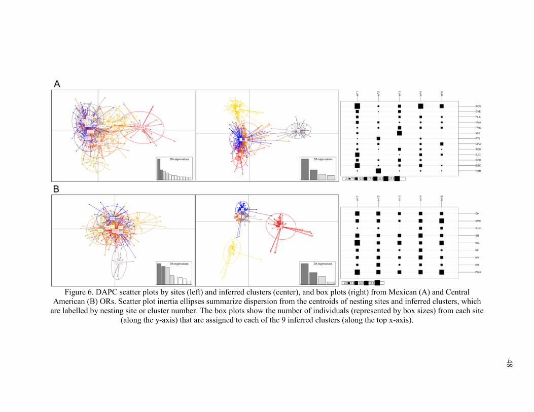
Figure 6. DAPC scatter plots by sites (left) and inferred clusters (center), and box plots (right) from Mexican (A) and Central American (B) ORs. Scatter plot inertia ellipses summarize dispersion from the centroids of nesting sites and inferred clusters, which

are labelled by nesting site or cluster number. The box plots show the number of individuals (represented by box sizes) from each site (along the y-axis) that are assigned to each of the 9 inferred clusters (along the top x-axis).

48

Figure 7. Diagrams of relative migration calculated by divMigrate (Sundqvist et al. 2016) between NWCR sites and behaviors (A-C) and DAPC clusters (D-F). Migration was inferred using Nm (A, D; Alcala et al. 2014), Gst (B, E; Hedrick and Goodnight 2005), and D (C, F; Jost 2008) over 1000 bootstrap replicates. Arrows represent migration between sites, and numbers at each arrowhead indicate the potential for migration (on a 0 to 1 scale) to the site nearest the arrowhead from the site at the other end of that arrow. Bold values

indicate significantly asymmetric migration between sites (alpha=0.05). Arrow coloring is intended only as a visual aid.

49

50

Figure 8. Diagrams of relative migration calculated by divMigrate (Sundqvist et al. 2016) between ETP sites, shown as circles. Migration was inferred using Nm (A; Alcala et al. 2014),

Gst (B: Hedrick and Goodnight 2005), and D (C; Jost 2008) over 1000 bootstrap replicates. Arrows represent migration between sites, and numbers indicate the potential for asymmetric

migration (on a 0 to 1 scale) between sites. The color of each arrow is indicative of the level of migration between sites, from low (light blue) to high (dark blue). The proximity of the circles to

one another is dictated by the level of migration between circles, from low (distant) to high (near). Sites are only shown with significant asymmetric migration.

51

Figure 9. Diagram of relative migration calculated by divMigrate (Sundqvist et al. 2016) between ETP clusters, shown as circles. Migration was inferred using Nm (A; Alcala et al.

2014), Gst (B: Hedrick and Goodnight 2005), and D (C; Jost 2008) over 1000 bootstrap replicates. Arrows represent migration between sites, and numbers indicate the potential for

asymmetric migration (on a 0 to 1 scale) between sites. The color of each arrow is indicative of the level of migration between sites, from low (light blue) to high (dark blue). The proximity of

the circles to one another is dictated by the level of migration between circles, from low (distant) to high (near). Sites are only shown with significant asymmetric migration.

A)

Figure 10. Unrooted neighbor-joining trees of NWCR individuals constructed using Da (A; Nei et al. 1983) and Fst (Latter 1972) over 1000 bootstrap replicates. Bootstrap values are represented by branch color. Tips are labelled with each individual, which nesting site

they were sampled at, and to which DAPC they correspond.

52

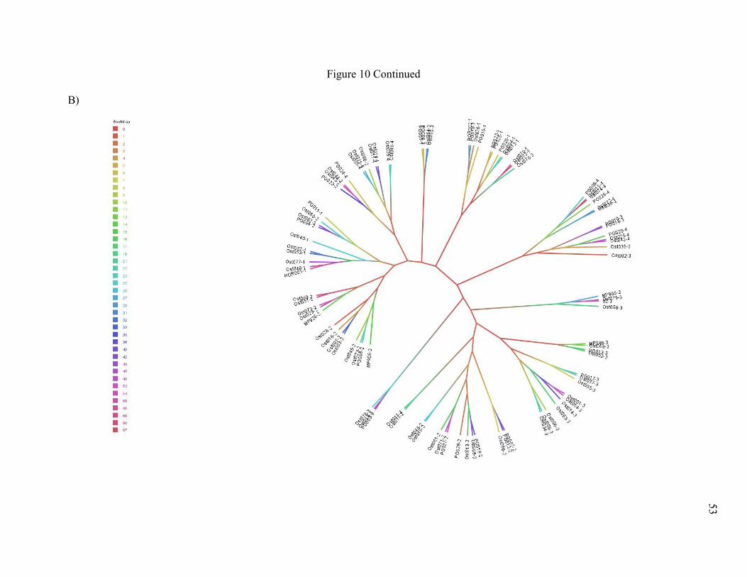
Figure 10 Continued

B)

53

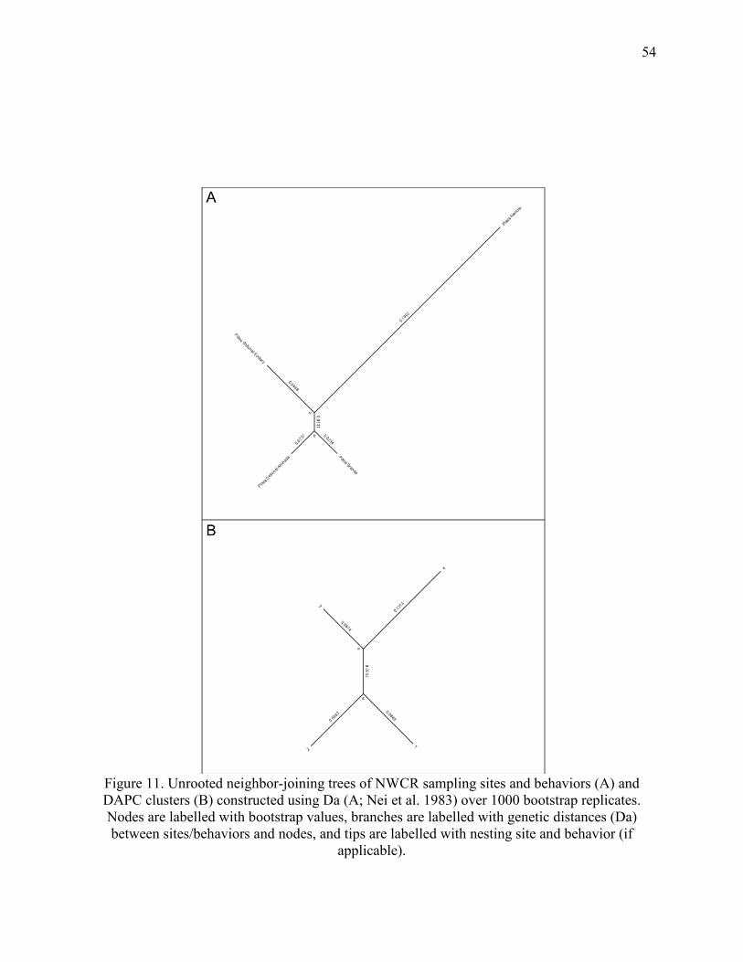
54

Figure 11. Unrooted neighbor-joining trees of NWCR sampling sites and behaviors (A) and DAPC clusters (B) constructed using Da (A; Nei et al. 1983) over 1000 bootstrap replicates. Nodes are labelled with bootstrap values, branches are labelled with genetic distances (Da) between sites/behaviors and nodes, and tips are labelled with nesting site and behavior (if

applicable).

55

Figure 12. Unrooted neighbor-joining tree of ETP individuals constructed using Da (A; Nei et al

1983) over 1000 bootstrap replicates. Bootstrap values are represented by branch color. Tips represent individuals, but are unlabeled. Pie charts represent the proportion of individuals present

from each DAPC cluster (1-9) in ad hoc clades, denoted on the tree by black stars. Sub-clades (i.e. stars following another star) have individual pie charts. Pie charts are located adjacent to the

clades they represent.

56

Figure 13. Unrooted neighbor-joining tree of ETP sampling sites constructed using Da (A; Nei et al. 1983) over 1000 bootstrap replicates. Bootstrap values are represented by branch color. Tips

are labelled with sampling sites.

57

Figure 14. Unrooted neighbor-joining tree of ETP DAPC clusters constructed using Da (A; Nei

et al. 1983) over 1000 bootstrap replicates. Bootstrap values are represented by branch color. Tips are labelled with DAPC cluster numbers.

58

DISCUSSION

Overview

This study was designed to answer 4 questions regarding NWCR and ETP OR population

structure, and regarding the utility of population inference methods in general.

Question 1: Would mtDNA analysis support or refine population structure in NWCR and ETP

ORs?

Analyses of mtDNA did not support or refine population structure in NWCR or ETP

ORs. mtDNA did not suggest structuring between or within NWCR sites or differing behaviors,

which confirmed Koval’s (2015) findings of NWCR ORs belonging to one larger population. I

was unable to compare our data set with a data set from Mexican ORs (Lopez-Castro and Rocha-

Olivares 2005) due to issues detailed below, but it is possible that divergences within NWCR

ORs and among ETP ORs are too recent to be detected in mtDNA haplotype data.

Question 2: Would analysis of ETP OR nDNA elucidate substructuring within Mexican

and/or Central American populations?

Analysis of ETP OR nDNA elucidated substructuring within Mexican and Central

American OR populations. In the ETP, hierarchical Bayesian analysis suggested weak structure

within Mexican ORs, and weak, cryptic structure in Central American ORs (Figure 3). In

Mexico, there is evidence that PAR may comprise a unique subpopulation (Fst=0.067), while in

Central America population structure may not be easily related to nesting locations.

STRUCTURE analysis of the entire ETP and of Mexican ORs did not strongly suggest this

partitioning, which was highlighted by DAPC.

Ordination confirmed and possibly refined hierarchical STRUCTURE results. DAPC of

ETP ORs by nesting site highlighted the singular nature of PAR ORs and refined that putative

population (Figure 4A). DAPC by most likely groupings found nine clusters which largely

corresponded to Mexican and Central American populations, but contained individuals from both

populations (Figure 4B). Individuals nesting primarily at PAR and PTI comprised a unique

59

cluster separated from all other ETP ORs. This, as well as the near-even distribution of Central

American ORs into 5 clusters, follow results of hierarchical Bayesian inference.

Question 3: Would DAPC produce cryptic clusters in both NWCR and ETP ORs?

DAPC produced cryptic clusters in both NWCR and ETP ORs. DAPC clusters from the

ETP spanned multiple nesting beaches and were particularly admixed between sites in Central

America (Figure 4B). It is impossible to determine if NWCR ORs would fit into the ETP DAPC

clusters as the two data sets cannot be merged without extensive allele size calibration. I discuss

possible explanations for this cryptic clustering in discussions of Ecological and Conservation

Significance below.

Question 4: What processes might be contributing to the formation of inferred populations,

and which inferred populations were best supported by multiple analyses?

Bottleneck events, related groups of individuals, and differential migration all contributed

to the formation of inferred populations. Populations inferred in NWCR and the ETP using

ordination were most consistently and strongly supported by all analyses, while populations

inferred by Bayesian inference were less consistently and more weakly supported by all analyses.

Genetic Distance Analysis

The NJ tree of NWCR individuals showed that individuals grouped primarily by DAPC

cluster, and indicated more support for DAPC groupings than for nesting sites/behaviors. As

with NWCR ORs, ETP individuals in the NJ tree were grouped broadly by DAPC clusters, and

there was higher bootstrap support for DAPC clusters than for nesting sites in those NJ trees,

respectively. NJ trees do not appear to have the same power as Bayesian inference or ordination

in inferring broad population structuring, as suggested by low bootstrap values at the base of

most NJ trees presented here.

Bottleneck Analysis

Inferred structuring may have been due in part to bottleneck events. Bottlenecks were

detected overall in both Mexico and Central America (Table 5), which supports inference for

those two populations. This confounds Rodriguez-Zarate et al.’s (2018) findings of “isolation by

60

environment,” as bottlenecked populations may have unique genetic signatures (Piry et al. 1999,

Putman and Carbone 2014). In ETP ORs, isolation by environment may play a role in population

structuring by facilitating or limiting gene flow and migration between sites and inferred

populations. However, bottleneck events (particularly in Mexico) have likely contributed the

formation of the Mexican population, and to the formation of subpopulation within Mexico.

Bottlenecks were detected at 9 continental nesting sites (7 in Mexico; 2 in Central

America; Table 5). Bottlenecks detected at continental sites may be due to historically intense

fishing pressure, harverst, and nest-site poaching, particularly in Mexico (i.e. Marquez et al.

1996). The bottleneck at PAR may have been severe enough to cause differentiation of that site

from all other ETP sites. However, asymmetric migration may confound some bottleneck

estimates (see Sundqvist et al. 2016 and references therein). PAR was identified as a possible

population sink, which may confound bottleneck testing and might have caused PAR to display a

unique signature in population structuring inference. Bottlenecks detected at BCS confirm

findings of the Baja Peninsula as a unique population that may warrant designation as a unique

MU (i.e. Lopez-Castro and Rocha-Olivares 2005, Rodriguez-Zarate et al. 2013).

Bottleneck events were not detected in NWCR or at all ETP sites. This may be due to a

lack of bottlenecking at these sites or population recovery past the point of detecting bottlenecks

at these sites. This may also be due to the limits of bottleneck metrics and software, specifically

in their sensitivity to parameter inputs as seen in this study (Table 6; Putman and Carbone 2014).

Migration was found to be significant from Mexico to Central America (Table 8), and it is

possible that Mexican ORs are contributing to genetic rescues at Central American sites where I

did not detect bottleneck events (Ingvarrson 2001).

Bottlenecks were detected by the two-tailed Wilcoxon test in 6 out of 9 ETP DAPC

clusters (3 in Mexico, 3 in Central America. Table 5). It is difficult to determine exactly what

might be leading to genetic bottleneck signatures in the DAPC clusters since they contain

individuals from distant nesting beaches. However, many of the clusters with bottleneck

signatures also had significantly high Fis (Table 4). Low recruitment to clusters and mating

between related individuals might produce bottleneck-like signatures, and this paradigm may

have even been engendered by bottleneck events. I might also expect these results (bottleneck

signatures and inbreeding) if the clusters reflect mating behaviors (see discussion of Ecological

Significance below), and if ETP ORs display mating site fidelity.

61

Relatedness Analysis

Structuring, especially cryptic clustering in DAPC, may be explained by mating patterns,

which could lead to high relatedness in clusters. In NWCR, relatedness was low across sites and

behaviors but high within DAPC clusters. It is possible that relatedness was low at sites due to

low nesting site fidelity in NWCR ORs. Sampling effort may also be suspect: if the NWCR OR

population is very large relative to other OR populations, and NWCR ORs are no more or less

fecund than ORs elsewhere, then the probability of sampling related individuals in NWCR will

be lower than it is elsewhere. Arribadas number in the tens of thousands, and sampling efforts

may have to be larger at arribada beaches to account for increased assemblage size.

Relatedness was higher at ETP nesting sites than at NWCR nesting sites and behaviors.

This may be an artefact of sampling and genotyping (see Blouin 2003), but could be due to

smaller populations outside of NWCR or higher natal site fidelity outside of NWCR. The latter

would be a difficult phenomenon to explain if it were true, but could be due to: a) the abundance

and proximity of nesting beaches, particularly arribada beaches, and a possible lack of

evolutionary pressure to home to natal beaches in NWCR; b) pressure to avoid competition for

suitable nesting habitat by nesting outside of NWCR; and/or c) low magnetic declination near

NWCR leading to navigational miscalculations by nesting turtles (i.e. Brothers and Lohmann

2018).

Relatedness may serve as an indicator of nesting-site fidelity. Relatedness was low at

sites and overall in NWCR. Relatedness in Central American ORs overall was higher than

relatedness at Central American nesting sites on average, while relatedness in Mexican ORs

overall was lower than relatedness at Mexican nesting sites on average. Nesting beaches in

Mexico may partition related individuals better than the overall sample, which may be explained

by natal site-fidelity. In Central America, individuals may display lower site fidelity, and thus the

relatedness signature at nesting beaches is lower than for the overall population. This lowered

site fidelity could explain the negligible relatedness signatures at NWCR nesting sites. Further,

relatedness was higher in Central America overall than in Mexico overall. Central American ORs

may generally display lower site fidelity than Mexican ORs, but be more-recently established,

hence higher overall relatedness within the Central American population.

Relatedness was comparable between DAPC clusters and nesting sites in the ETP, as well

as Mexican and Central American populations. In many cases, DAPC relatedness was higher

62

than relatedness in putative populations or at nesting sites. While it is possible that the DAPC

clusters result from related groups of individuals, if this were the case then DAPC might have

suggested at least some individual nesting sites (such as PAR) as unique clusters. This, as well as

moderate-strong signatures of divergence mentioned above (i.e. pairwise Fst and D, and

AMOVA) suggest that the DAPC clusters are not artefacts of analysis but true groupings of

individuals as a result of some evolutionary process(es). It may also lend support to the DAPC

clusters as more effective population groupings for ETP ORs than STRUCTURE clusters (see

discussion of Bayesian inference and ordination below).

Migration Analysis

Migration was comparable between NWCR sites/behaviors, but uneven between DAPC

clusters. Migration indicated significant asymmetric gene flow between Mexican and Central

American ORs, and highlighted specific source (MIS) and sink (PAR) populations. Migration

was present between sites throughout the ETP, not solely within Mexico and Central America.

Migration was limited between Mexican DAPC clusters, but significant between Central

American clusters and from Mexican clusters to Central American clusters. This information is

important for effective management of ETP ORs, and was not evident from Bayesian inference

alone. DAPC grouped individuals from Mexico in primarily Central American clusters and vice-

a-versa; these individuals may in fact represent recent migrants between the two populations.

However, individuals from MIS (the primary source population in the ETP) were not often

clustered with Central American individuals after DAPC.

NWCR OR mtDNA

Chelonian mitochondrial DNA has been shown to accrue mutations on a scale of tens of

thousands to hundreds of thousands of years. Past phylogeographic studies of ORs have

suggested that the EP population is no more than 250,000-300,000 years old (Bowen et al. 1997,

Jensen et al. 2013B). Thus, while at least 14 control region haplotypes are reliably documented

from EP ORs (Bowen et al. 1997, Lopez-Castro and Rocha-Olivares 2005, Jensen et al. 2013B),

it is likely none have established themselves at a level similar to the basal haplotype (Lo46;

Bowen et al. 1997, Lopez-Castro and Rocha-Olivares 2005, this study) despite evidence for

population structuring (Rodriguez-Zarate et al. 2018). However, I found Lo46 at a slightly lower

63

rate in NWCR ORs (~70%) than has been reported for Mexican ORs (~90%; Lopez-Castro and

Rocha-Olivares 2005). Lopez-Castro and Rocha-Olivares (2005) posited that the Baja Peninsula

nesting population is basal to EP ORs given the high presence of Lo46. It is possible then that

the lower rate of Lo46 found here in NWCR ORs may be characteristic of environmental

partitioning between Mexican and non-Mexican ORs (Rodriguez-Zarate et al. 2018).

This hypothesis cannot be tested without an organized and complete global database of

OR haplotypes and accurate and complete reporting of haplotype datasets. Haplotype frequencies

at different sites may be compared using pairwise F-like statistics (i.e. Φst and 𝚯𝚯st; Wright 1949,

Weir and Cockerham 1984) and AMOVAs (Excoffier et al. 1992) given complete datasets and

corresponding sequences. Sequences from published studies should be retrievable from

Genbank, and reported haplotype frequencies may then be reconstructed to test population

differentiation hypotheses. When I attempted to do so for ETP ORs, I found serious

discrepancies, ambiguities, and author-oversight in naming and reporting of haplotypes not just

for ETP ORs but for ORs globally.

There are two databases that contain OR haplotypes: Genbank, and a database maintained

by the National Marine Fisheries Service (NMFS; Peter Dutton, personal communication).

Haplotypes on Genbank (n=45 as of this study) are publicly available but are not organized

between studies. Many studies use the alphanumeric nomenclature first established by Bowen et

al. (1997), but some use unique names for their sequences (see below). Haplotypes in the NMFS

database (n=96 as of this study) are named sequentially from when they were provided to NMFS

(i.e. Lo1, Lo2; see below), and are not publicly available, but some haplotypes named using the

NMFS system are listed on Genbank (see Jensen et al. 2013B). Haplotypes presented in this

study are named using the NMFS system, since the NMFS database is more complete than

Genbank.

There are further issues with reported haplotypes: some reported haplotypes are not

publicly available; some papers use multiple nomenclatures to describe single haplotypes; and

some publicly available haplotypes are listed under different names than were reported in their

original publication, sometimes sharing the same name with a different haplotype. For example,

haplotypes Q-W are reported from ETP Olive ridleys (Lopez-Castro & Rocha-Olivares 2005) but

are unavailable from Genbank and there is no polymorphic-site data to allow for manual

64

reconstruction of these haplotypes. This prevented us from using our mtDNA data to look for

evidence for population structuring between Mexican and non-Mexican EP ORs.

Haplotype N (NMFS Lo46; Accession #’s AF051776 & AF514311; Bowen et al. 1997, Shanker

et al. 2004B) is the most abundant haplotype known for EP Olive ridley turtles and was first

reported at ~400bps (Bowen et al. 1997, Lopez-Castro & Rocha-Olivares 2005). However, on

Genbank the ~800bp haplotype that matches the ~400bp haplotype “N” is labelled “K”

(Accession # AY920519), identical to a haplotype “K” that is known only from the Indian

population (Bowen et al. 1997, Shanker et al. 2004B). Further, the ~800bp haplotype labelled

“N” (Accession # AY920521) matches the ~400bp haplotype “O” as described by Bowen et al.

(1997).

Nearly every publication reporting OR haplotypes utilizes a unique naming system, in

addition to the original haplotype names assigned by Bowen et al. (1997; Table 2). Shanker et al.

(2004B) reported five haplotypes stemming from haplotype “K” (Bowen et al. 1997) in India.

These haplotypes were named K-1 thru K-5. Jensen et al. (2013B) reported over 20 new

haplotypes from IP turtles using NMFS conventions and explicitly stated which ~800bp

haplotypes corresponded with ~400bp haplotypes reported by Bowen et al. (1997). Bahri et al.

(2018) used the NMFS formula (seemingly without consulting NMFS) for naming sequences

deposited in Genbank from Indonesian ORs. While Jensen et al. (2013B) used “Lo2” to name the

~800bp sequence that overlaps with the ~400bp sequence named “G” by Bowen et al. (1997), the

~800bp “Lo2” reported by Bahri et al. (2018) is entirely unique.

The lack of consistent, systematic haplotype naming is a preventable obstacle, yet there

seems to be no inertia to push studies to systematically name haplotypes or to deposit unique or

named haplotypes in Genbank (i.e. Plot et al. 2012, Bahri et al. 2018). mtDNA D-loop haplotype

nomenclatures exist for Loggerhead (Caretta caretta) and Green (Chelonia mydas) sea turtles

(i.e. http://accstr.ufl.edu/resources/mtdna-sequences/), Leatherback sea turtles (Dermochelys

coriacea; Dutton et al. 1999, Dutton et al. 2013), and Hawksbill (Eretmochelys imbricata;

Leroux et al. 2012) sea turtles. Researchers and managers are increasingly focusing on Olive

ridley population structure, and such studies will benefit from a consensus, global nomenclature

for Olive ridley control region haplotypes. It has been 20+ years since the last global

phylogeography of ridley turtles (genus Lepidochelys) was published (Bowen et al. 1997), and a

65

new effort to study ridley phylogeography will necessitate better organization of mtDNA

haplotypes.

Bayesian Inference vs. Ordination

Bayesian inference (BI), as implemented in STRUCTURE (Pritchard et al. 2000) proved

useful at highlighting population structure on the scale of the entire ETP. However, I was unable

to detect population structuring at the same resolution using BI as with ordination, as

implemented in adegenet (Jombart et al. 2008). I was specifically unable to detect differentiation

between PAR and other sites (which was confirmed by F-statistics, AMOVA, and ordination)

without hierarchical analysis in BI. While it is possible that PAR comports a false signature of

differentiation as a putative population sink, analysis using BI alone did not identify this

possibility and would have perhaps lead to incorrect conservation efforts at PAR (see

Conservation Significance below).

Population inference using STRUCTURE may have been limited by assumptions of

Hardy-Weinberg equilibrium (HWE) and an inability to account for high levels of admixture

between sites, particularly in the southern ETP. The presence of three linked loci in the CR

dataset lowered resolution from eight loci to six loci when analyzing population structure using

BI (Koval 2015). It is possible that including more than six loci would have allowed me to detect

more than one population in NWCR ORs using STRUCTURE. Even with more loci, as in the

EP-wide dataset, hierarchical analysis of STRUCTURE results did not elucidate discrete

populations in the southern ETP, and only slightly resolved structure in Mexican ORs by

highlighting the unique genetic signature of turtles nesting at PAR.

STRUCTURE and DAPC allowed me to detect broad divisions between Mexican and

Central American ETP ORs, but inference using DAPC suggested finer-scale population

structuring that inference in STRUCTURE did not suggest. Inference in STRUCTURE should in

theory suggest these groups, as it performs well to identify populations with Fst≥0.02 (Latch et

al. 2006). Inference in STRUCTURE may have been unable to elucidate within-subpopulation

structuring due to the clustering method and assumptions programmed into STRUCTURE.

STRUCTURE is based on the theory that alleles within established natural populations will be in

HWE. This presumption, briefly stated, means that relative allele and genotype frequencies at

each locus should not deviate from expected frequencies. STRUCTURE uses a Bayesian model

66

and Gibbs sampling of a Monte-Carlo Markov Chain of simulated populations (K) to look for

groups of individuals with loci in HWE (Pritchard et al. 2000). In this context, the probability of

seeing my data (X) given groups of individuals (Z) with unique genetic signatures (P; P(X|Z,P))

may then be used (via ad hoc methods) to estimate the best K. Thus, for K=2, individuals fit into

1 of 2 ancestral populations (excluding admixed individuals) with different allele frequencies.

The assumption of populations with different allele frequencies that are in HWE may not

be appropriate for all data (Pritchard et al. 2000, see examples in Kalinowksi 2011 and Putman

and Carbone 2014). HWE arises when gene-flow between populations is minimal.

STRUCTURE implements algorithms to account for admixture and migrant individuals

(Pritchard et al. 2000), and populations with correlated allele frequencies (Falush et al. 2003), but

only when both occur at relatively low levels (i.e. probability of migration = 0.001-0.1; Pritchard

et al. 2000). In both data sets analyzed here, clusters identified by DAPC did not have allele

frequencies that differed notably from parent populations (i.e. overall in Koval 2015, and

Mexican and Central American in Rodriguez-Zarate et al. 2018). This could be due to gene flow

between clusters in both data sets, particularly in Central American ORs. STRUCTURE may

also require many loci (i.e. 200-300) and a certain minimum number of non-migrant or non-

admixed individuals to recognize numerous migrant and admixed individuals (Pritchard et al.

2000). Low-enough levels of admixture for STRUCTURE to define K may only occur at a broad

scale (i.e. Mexican vs non-Mexican sites) in ETP ORs. High migration between Central

American clusters may have lowered the likelihood cost of STRUCTURE grouping all Central

American sites together, rather than clearly identifying DAPC-like clusters (i.e. Kalinowski

2011; see below).

While inference in STRUCTURE distinguishes sea turtle populations on a broad scale

(i.e. Rodriguez-Zarate et al. 2018), sea turtles may exhibit levels of intra-population gene flow

and migration that exceeds STRUCTURE’s capabilities on finer scales. All sea turtles display

some level of natal breeding philopatry (Lohmann et al. 2017), in which they return to the region

that they originated from to breed. Female turtles may even return to the exact beach from which

they hatched to lay their own nests. Male sea turtles, not limited by the need for a nesting beach,

are known to show limited natal breeding philopatry relative to female sea turtles. Studies that

examine both mtDNA and nDNA from the same individual nesting females may find more

evidence for structuring with mtDNA than with nDNA (FitzSimmons et al. 1997, Roberts et al.

67

2004), which suggests males may breed with multiple females from relatively distant nesting

beaches. This could confound clustering in STRUCTURE, as any sampled female may have

been fathered by an unsampled male that might have originated from a different population (or

nesting area). Further, female natal beach site-fidelity is thought to be limited in ETP ORs (Kalb

1999), and any female at one nesting beach may have originated from a more distant nesting

beach. This seems to be the case in NWCR ORs and non-Mexican ORs especially, as relatedness

values within sampling sites were negligible (NWCR) and less than relatedness within Mexican

nesting sites (ETP: Central America). Multiple sources of admixture between potential

subpopulations such as DAPC clusters (i.e. admixed heredity and low site fidelity) could have

led analysis of STRUCTURE results to suggest the most likely K=2.

As hinted at above, the lack of male genetic information in both data sets is problematic.

Due to natal breeding fidelity, we assume that sea turtle populations should be structured around

nesting beaches. The samples here consist of female nesting turtles with putatively limited natal

breeding fidelity, who are offspring of females with putatively limited natal breeding fidelity and

males with perhaps even more limited natal breeding fidelity. Further, since female ORs are

thought to reach sexual maturity at 10-15 years of age (Zug et al. 1998) and display varied

reproductive phenology (breeding remigration of 1-2 years; Kalb 1999, Dornfeld et al. 2015), the

females sampled here are likely offspring from different reproductive seasons, each comprised

by different individuals with different genetic makeups. Perhaps a more appropriate sampling

regime for future population studies would be to sample hatchlings from nests from the

geographic range of the study. This would provide more information towards identifying

contemporary admixture and structure based on all breeding individuals, and would not be biased

towards males or females (as hatchling sex may not be identified based on external morphology).

In determining the most likely K, STRUCTURE may settle on local likelihood maxima

and choose mathematically cost-effective structuring schemes in favor of real, yet less-cost-

effective schemes (Pritchard et al. 2000, Kalinowski 2011). Kalinowski (2011) showed this with

simulated hierarchical populations. In ETP ORs, STRUCTURE may be correctly identifying

Mexican and non-Mexican populations, but ignore finer-scale structuring. In analysis of the

Mexican population alone, analysis of STRUCTURE results identifies PAR as a unique

population, but groups all other sites together. DAPC results also identify individuals from PAR,

and PTI, as members of a unique cluster. A neighbor-joining tree of all ETP sites confirms the

68

Mexican/non-Mexican split, but also provides evidence for hierarchical structure within the

Mexican population. PAR and PTI, the two sites that comprise DAPC cluster #8, are most-

closely related to a clade that includes PVG, CPA, and TCO. The NJ tree also groups EVE, MIS,

and BCR (DAPC cluster #5) and BCS, PLA, SJC, and ESC (DAPC clusters #1 & 9) together.

The PAR-PTI clade may be preventing STRUCTURE from identifying other relationships

between nesting sites, as in simulated populations in Kalinowksi (2011).

ETP ORs might be thought of in the same framework as simulated populations in

Kalinowski (2011). STRUCTURE has two options: 1) separate PAR from Mexican and Central

American ORs such that K=3; or 2) include PAR in the Mexican population such that K=2.

STRUCTURE confers a likelihood penalty for increasing K to 3 for PAR, but also confers a

likelihood gain for resolving population structuring. On the other hand, STRUCTURE confers a

likelihood gain for inferring only 2 populations, but might confer slightly less of a gain for

including PAR in the Mexican population even though PAR has a unique genetic signature.

When all is summed, it may be more “cost-effective” for STRUCTURE produce results that

infer K=2 rather than 3.

Analyzing data hierarchically within STRUCTURE (i.e. the entire ETP, then just

Mexico, then just Central America) can elucidate such population structuring, but with each level

of analysis comes decreased analytical power through the loss of individual genotypes and

potentially some alleles. Additionally, it is difficult to know at which level it is appropriate to

cease such an analysis. After analyzing Mexican sites separately, is it appropriate to remove PAR

and repeat the analysis? It would not seem so based on STRUCTURE bar plots, since individuals

were still not completely assigned to the PAR group, and individuals at other sites were also

admixed. F-statistics and AMOVA would suggest removal of PAR and re-analysis, but they do

not operate within the STRUCTURE framework and it is not necessarily appropriate to force

population inference in STRUCTURE based on results from external analyses.

Population inference in DAPC detected fine-scale, cryptic structuring in both NWCR and

ETP ORs. In DAPC, genotypes are decomposed into coordinate data via PCA. DAPC then uses a

k-means clustering algorithm to delineate clusters, the most likely of which is determined using a

Bayesian Information Criterion (BIC). As implemented in DAPC, k-means and BIC identify the

most likely K as having the least within-group variance while penalizing higher values of K. The

assumptions, implications, and limits of DAPC are not well known (Putman and Carbone 2014).

69

Jombart et al. (2010) concede that k-means may not detect the correct clusters in complex

situations, and that some clusters may be artefacts of the algorithm. Another issue is the ad-hoc

implementation of DAPC, in which the user chooses how much % variance and how many

principal axes to retain. Here, I follow Jombart et al.’s (2010) suggestions for retaining %

variance and principal axes, and perform cross validation (within adegenet) to minimize error

when retaining principal axes. However, there remains subjectivity in balancing discriminatory

power and overfitting clusters (i.e. through retaining more principal axes; Jombart et al. 2010).

DAPC has been shown to outperform STRUCTURE in inferring clusters in populations

with complicated structuring, such as with hierarchical-island and hierarchical-stepping stone

models (Jombart et al. 2010). In the first model, random-mating subpopulations are confined to

“islands”. There is gene flow within and between islands, but the latter is of less magnitude than

the former. In the second model, random-mating subpopulations are confined to distinct zones.

There is gene flow between adjacent subpopulations within each zone, and limited gene flow

between zones, typically at a point of contact. In simulated populations with these models (K=6

and 12, respectively), STRUCTURE predicted K= 2 and 3, respectively. DAPC predicted K=6

and 11 respectively.

Hierarchical structuring may be occurring in ETP ORs, thus explaining branching in the

NJ trees and the clusters detected by analysis of DAPC results and not STRUCTURE results. Sea

turtle populations may not fit standard island or stepping stone hierarchical models. A

hierarchical stepping stone model might be appropriate for sea turtles assemblages with high

breeding site fidelity, in which females nest very close to their natal beach, and where females

and males only mate near their natal beach. Then, along a stretch of coast, there should be

genetic variation along a gradient and some gene flow between adjacent nesting assemblages.

This is the case for loggerhead turtles (Caretta caretta) nesting in the western Atlantic ocean,

which display mitochondrial variation along a gradient from Virginia, USA to south Florida,

USA, and then around the Florida panhandle into the Gulf of Mexico (Shamblin 2012) In the

ETP, such a pattern might be disrupted by environmental factors near the interface between

Mexican and Central American nesting beaches (Rodriguez-Zarate et al. 2018). However, while

relatedness values suggest some level of fidelity to nesting sites across the ETP, migration

appears to be minimal between relatively adjacent beaches in Mexican and Central American

ORs (Table 7).

70

The hierarchical island model, in which multiple subpopulations comprise broad,

relatively genetically isolated populations, may be better suited for ETP ORs, but perhaps not

purely by nesting site. Migration is present (sometimes at comparable levels) between all sites,

not only between adjacent sites within Mexican and Central American populations, and is

significant from some Mexican sites to Central American sites (Table 7). Migration is also lower

between Mexican clusters and between Mexican and Central American clusters than it is

between Central American clusters (Table 9). In a true hierarchical island population, migration

is expected be highest between subpopulations within broad populations, but not between broad

populations. This suggests that DAPC may have elucidated randomly mating subpopulations

with minimal gene flow in Mexico, at least. However, migration is high between non-Mexican

clusters, which may be due to relative panmixia or recent divergence in non-Mexican ORs, even

when separated by site or cluster. This is not to shed doubt on the non-Mexican clusters, but

rather suggests that they are not as discrete as Mexican clusters, which were even weakly

detected by STRUCTURE (ie PAR, cluster #8).

Thus, ETP ORs may comprise as many as 9 discrete genetic units. These units are

generally split into Mexican and Central American groups, but do not strictly adhere to Mexican

and Central American populations. There is evidence for significant gene flow between nesting

sites and all 9 groups in the ETP, particularly within Central America and from Mexico to

Central America. The Mexican clusters (1, 5, 8, 9) may comprise discrete populations in a

hierarchical island model, while the Central American clusters (2, 3, 4, 6, 7) may comprise

subpopulations of a broader Central American population in the same model.

STRUCTURE assumes that populations are in a state of relative isolation and

equilibrium, especially across broad distances, and does not perform well in identifying

hierarchical structuring. ETP ORs, and many other sea turtle populations in general, may not fit

STRUCTURE’s assumptions well-enough for analysis of STRUCTURE results to accurately

suggest populations. DAPC may be better suited for analyzing population structure in sea turtles,

which are highly migratory, have enormous potential for broad migration and genetic

connectivity, and may in many cases be recovering from anthropogenic bottleneck events. This

is supported with the weight of bottleneck, relatedness, migration, and phylogenetic analyses.

71

Ecological Significance

Population inference in DAPC elucidated genetically discrete clusters in ETP ORs that

may have formed from bottleneck events, family lineages, and/or cryptic mating behaviors. Sea

turtle populations declined globally in the 19th and 20th centuries due to fisheries impacts

(Lewison and Crowder 2007), as well as legal and illegal take of turtles for consumptive use

(Valverde et al. 2012, Foran and Ray 2016). This is true for the ETP, where legal take of OR

eggs is still allowed at Playa Ostional, and sporadic poaching of females and eggs still occurs

range-wide. ETP OR populations have begun to recover since the mid-20th century (Abreu and

Plotkin 2012), although some assemblages are thought to be in decline (Fonseca et al. 2009), and

in some cases entire arribada nesting assemblages have been lost (see Marquez et al. 1996).

Such bottleneck events may leave detectable genetic signatures, as was the case in some

ETP sites, putative populations, and DAPC clusters (discussed in Conservation Significance

below). However, not all sites and clusters displayed bottleneck signatures. At nesting sites

structuring and relatedness may be due to site fidelity (see above). In DAPC clusters without

bottleneck signatures, it is possible that family lineages contributed to contemporary structuring.

If certain limited lineages were reproductively successful during the peak of sea turtle take in the

ETP, descendants of these lineages could comprise contemporary ETP ORs. As those

descendants reached sexual maturity, they could have nested with limited natal site fidelity over

generations, perhaps constrained by oceanographic features (i.e. Rodriguez-Zarate et al. 2018,

see below). DAPC may have detected such lineages, which could explain the relatedness of

turtles within clusters.

Since oceanographic features are known to play a role in genetic structuring at the scale

of the entire ETP (Rodriguez-Zarate et al. 2018), perhaps they also play a role within Mexican

and Central American populations. If minor oceanographic features are more prominent offshore

of Mexico than offshore of Central American countries, descendants of bottlenecked lineages

may have been structured, and may continue to be structured, more so in the Mexican population

than in the Central American population, hence the low levels of migration detected between

Mexican clusters. In Central American ORs, oceanographic currents may not prevent migration

and may even facilitate it, thus explaining the connectivity between clusters and relatively low

levels of relatedness at nesting sites. Connectivity between Mexican and Central American ORs

may be dictated by broad scale currents such as the California Current and Equatorial Currents.

72

Baja California del Sur, MX (BCS) ORs are found in every Central American DAPC cluster, and

individuals from Mismaloya, MX (MIS) may migrate as far south as Panama (PMA). It is

possible that some of these putative migrants may have followed the California Current south

from Mexico, and then been directed to Central America via the Equatorial Counter Current

and/or Costa Rica Coastal Current (see Figure 1a in Rodriguez-Zarate et al. 2018).

The clusters could be due to contemporary genetic structuring through mating at discrete

locations. Little is known about the specific locations where sea turtles mate (Rees et al. 2016).

Although some mating occurs offshore of nesting beaches, it may occur elsewhere, such as on

migratory routes between foraging and breeding areas, and perhaps even at foraging areas. Sea

turtles tend to display multi-year fidelity to foraging grounds (Broderick et al. 2007, Schofield et

al. 2010). If turtles utilize discrete, even if broad, foraging grounds and mating occurs at or en

route to foraging or breeding grounds, I may expect to observe structuring that corresponds to

foraging regions. ETP ORs are thought to be nomadic foragers with broad foraging ranges

(Eguchi et al. 2007, Plotkin 2010), but comprehensive data on foraging ETP ORs, such as home

range estimates from telemetry data and stable isotope values, do not exist. If ETP ORs display

some level of fidelity to broad foraging regions and mating occurs at foraging grounds or

between foraging and nesting grounds, then it may contribute to the structuring detected by

DAPC. However, more data are needed to investigate correlations between genetic structuring

and trophic and spatial ecology of ETP ORs.

There was not strong evidence to suggest that ordination captured specific migration

patterns between sites and putative populations. Although clusters contained individuals from

both populations, they did not always contain individuals from a significant source population in

Mexico (MIS). DAPC may have unintentionally identified demographically discrete populations

with few immigrants in Mexico, but did not do so in Central America. DAPC clusters may

reflect deeper, or different, population structuring than can be captured in estimates of migration.

Conservation Significance

Conserving highly migratory, long-lived species such as sea turtles is a difficult

endeavor. Sea turtles occupy diverse habitats and shift habitats ontogenetically, and resources for

conservation efforts are limited. Time-series abundance data from nesting beaches and foraging

grounds may identify high-use areas, and conservation plans may focus on areas with the highest

73

density of turtles or areas experiencing declines in abundance. However, such plans do not

account for population connectivity and gene-flow that can only be elucidated by genetic studies.

For example, one foraging ground may contain turtles from three genetically discrete

populations. Although abundance data may indicate stability, genetic data may show that

individuals from one population are declining at that site. Such data allow researchers and

conservationists to investigate those declines and design plans to aid in population recovery.

Designating genetically discrete populations is therefore critical to effectively conserving

sea turtles, but it must be done so correctly and practically. Here, I show that population

inference in STRUCTURE only elucidates broad populations of ETP ORs, while DAPC

uncovers fine-scale structuring. ETP ORs are certainly split at the Mexican-Central American

interface (Rodriguez-Zarate et al. 2018), but there is important sub-structuring within these

populations and connectivity between these populations. Although the clusters are difficult to

explain, they merit investigation and conservation planning. The clusters may comprise MUs,

but MUs are typically spatially continuous groups of nesting assemblages. It may be more

appropriate to designate the clusters as Demographically Independent Populations (DIPs;

Komoroske et al. 2017). DIPs exhibit low levels of differentiation but comport conservation

importance (see Taylor et al. 2010, Dutton et al. 2013). DAPC cluster 8 provides one obvious

example of a putative DIP, although PAR alone might comprise an MU worthy of prompt

conservation planning. It is possible that each DAPC cluster may be a unique DIP, and should be

incorporated into management plans as such, especially after further investigation. This is a

challenging notion, but if the DAPC clusters could be related to mating at discrete foraging

grounds, protecting those areas could ensure the persistence of the DAPC clusters. Satellite

telemetry of post-nesting Olive ridleys will be crucial to determining the formation of the DAPC

clusters. Finding discrete high use areas that correspond with the DAPC clusters would add a

tangible, spatial element to population structure in ETP ORs that managers and conservationists

can protect by designating Marine Protected Areas, for example. Further, DAPC highlighted

connectivity between Mexican and Central American ORs (see Figure 4) that was confirmed by

migration estimates (Tables 7 and 9, Figures 8 and 9). This connectivity spans ~3,500 km as the

crow flies (between BCS and PMA), and can be affected if not interrupted by unregulated

fisheries and shipping industries. Management and conservation plans must account for this

broad connectivity. Knowledge of migratory routes and strategies used by ORs, gained via

74

satellite telemetry, will be important if there is to be effective conservation of ORs away from

nesting beaches.

Some of the putative DIPs showed evidence for inbreeding (Table 4) and bottleneck

events (Table 5). It should be of concern to managers and conservationists that these process

might be going on for genetically discrete populations of unknown origins across multiple,

distant nesting beaches. If recent or ongoing take is not occurring at nesting beaches, it may be

occurring elsewhere, such as at foraging grounds or along migratory routes. Although I did not

test for decreases in population size here, ORs are globally in decline (IUCN 2018). By focusing

conservation efforts on nesting beaches, managers and conservationists may be missing an

unidentified population outflow for ETP ORs. Concern should be highest in the Mexican

population of ETP ORs, where 3 out of 4 putative DIPs showed evidence of bottleneck events,

and all putative DIPs showed significant inbreeding.

Population inference using ordination, and not Bayesian inference, efficiently produced

well-supported groupings in ETP ORs that should be incorporated into conservation and

management plans, rather than results of Bayesian inference alone. Designing conservation plans

based solely on panmictic Mexican and Central American populations would be incorrect and

impractical. Monitoring even a majority of the nesting habitat in Mexico would be impossible,

and such a plan might suggest monitoring only beaches with the highest abundance of nesting

turtles. Monitoring away from nesting beaches (i.e. at foraging areas) is relatively expensive and

might seem wasteful in this scenario, since the turtles at any given beach all come from the same

genetic population and it should be possible to examine population trends for all Mexican ORs

by monitoring nesting beaches.

In Central America, a management plan for a panmictic population would require

cooperation from conservation entities from as many as 6 nations. When determining priority

areas for monitoring and protection, conservation efforts and funding in a regional management

framework might be biased towards nations with the highest abundance of nesting ORs, namely

Costa Rica and Panama (due to the presence of arribada beaches). Alternatively, each nation

might enact individual plans to monitor their own nesting beaches, eschewing standardization or

a regional conservation mindset. These scenarios may already be playing out, and the lack of

cooperation, standardization, and urgency in conserving ORs could be contributing to their

global decline (IUCN 2018).

75

Ordination, as implemented in DAPC, provides us with a higher-resolution picture of

population structure in ETP ORs than does STRUCTURE, and could allow for more practical

and effective management plans. Ordination highlights the presence of Mexican and Central

American populations, but highlights connectivity between both populations and of connectivity

and internal structure within both populations. Conservation plans based on ordination could

account for that connectivity and internal structuring, and could examine possible causes of

bottleneck events and inbreeding not strictly related to nesting sites. The PTI-PAR DIP is a clear

example of this. A conservation plan premised upon panmixia might not suggest monitoring at

PTI or PAR if other sites were more frequently used. Ordination highlights that turtles at those

sites are genetically unique and provides impetus for monitoring at those beaches. Further,

ordination provides impetus to investigate connectivity between PTI and PAR, as well as the

processes that form these putative DIPs in general.

Conservation at nesting beaches alone may not protect every genetically discrete group of

ETP ORs. Conservation at foraging grounds might be an important facet of a regional

conservation plan, if it would work towards preserving the PTI-PAR cluster and other putative

DIPs. Such a plan would also necessitate spatial and temporal investigations of mating behaviors

to better understand the DAPC clusters. If clusters do correspond to mating at specific sites or

regions, it may be possible to highlight those areas in conservation planning. These areas may

overlap with fishing grounds or shipping lanes, and policies could be implemented to mitigate

impacts from these industries on discrete clusters. Identifying these hotspots in waters belonging

to Central American nations might provide a useful framework for a regional conservation plan

for otherwise panmictic ORs. For example, if one of the clusters corresponds to turtles that are

found at a foraging ground off of Nicaragua, the country could enact policies to protect that

foraging ground. In doing so, they would likely protect turtles that nest along the entire Central

American coast and directly contribute to the conservation of the species as well as to preserving

a vast eco-tourism industry based on sea turtles (Delgado and Nichols 2005, Senko et al. 2011).

The clusters provide a more tangible path towards regional conservation than do panmictic

Mexican and Central American populations.

76

Conclusion

Sea turtles are difficult species to conserve due to their long migrations and broad

distributions. Defining MUs and other discrete population units such as DIPs around which to

base conservation plans must be done correctly to effectively conserve genetically discrete

populations of sea turtles. In this study, ordination provided a more practical and nuanced

framework for defining MUs and DIPs in ETP ORs than did STRUCTURE. This may be due to

hierarchical structuring within ETP ORs that may be present in other sea turtle populations and

species. In the case of ETP ORs, hierarchical structure may be an artefact of recent population

bottlenecks and subsequent recolonization of nesting beaches, or due to mating at foraging

grounds or along migratory routes.

It appears that population inference based on BI, such as is implemented in

STRUCTURE, may not be best suited for defining MUs and DIPs for sea turtles with

hierarchical structuring. Gene flow between distant breeding areas may lead to the violation of

critical assumptions made by programs using BI, namely that the most suitable discrete

populations display different allelic signatures, are in Hardy-Weinberg equilibrium, and are not

highly admixed. The “best” genetically discrete groupings of sea turtles may not always conform

to these constraints. Barriers that prevent gene flow may be relatively limited in the ETP and

marine environments generally (Hellberg et al. 2002), or may only be present at broad spatial

scales (i.e. Rodriguez-Zarate et al. 2018). Migration between genetically discrete groupings may

be common in sea turtles given their migratory nature, and perhaps even evolutionarily

advantageous (i.e. through genetic rescue; Ingvarsson 2001). Ordination makes no assumptions

about the characteristics of genetically discrete populations, and simply maximizes variance

between groups of the most genetically similar individuals.

Results from exploratory ordination must be carefully examined in the context of the

study system, and can be supplemented with analyses to understand how genetically discrete

groupings may have formed. Here I showed that ordination validated broad-scale population

structure, recognized gene flow between broad populations, and grouped related individuals

together within populations in what may represent DIPs not tied to nesting beaches. This

connectivity and lack of terrestrial structuring is feasible for sea turtles, was supported by

bottleneck, relatedness, and migration analyses, and merits investigation, both as an ecological

phenomenon and as basis for a management framework. Microsatellite data from previous

77

studies that relied only on BI of genetically discrete sea turtle populations should be re-analyzed

with ordination, and results should be compared between both methods and investigated to better

understand how these discrete groupings formed and interact with one another. Future studies

should always compare multiple exploratory (Bayesian inference, ordination, phylogenies) and

explanatory (bottleneck, relatedness, migration) methods for population inference. The outcome

may lead to at least subtle, but important, changes in the designation of MUs, DIPs, and

management plans for sea turtles globally, and could lead to a better understanding of sea turtle

biology and life history.

78

REFERENCES

Abreu-Grobois FA, Horrocks J, Formia A, Dutton PH, LeRoux R, Velez-Zuazo X, Soares L,

Meylan P (2006) New mtDNA Dloop primers which work for a variety of marine turtle

species may increase the resolution of mixed stock analyses Proceedings of the 26th

Annual Symposium on Sea Turtle Biology Isle of Crete, Greece, p 179

Abreu-Grobois A, Plotkin P (2012) Lepidochelys olivacea The IUCN Red List of Threatened

Species

Alcala N, Goudet J, Vuilleumier S (2014) On the transition of genetic differentiation from

isolation to panmixia: what we can learn from GST and D. Theor Popul Biol 93:75-84

Avise JC, Bowen BW, Lamb T, Meylan AB, Bermingham E (1992) Mitochondrial DNA

evolution at a turtle's pace: evidence for low genetic variability and reduced

microevolutionary rate in the Testudines. Mol Biol Evol 9:457-473

Bahri S, Atmadipoera AS, Madduppa HH (2018) Genetic Diversity of Olive Ridley

Lepidochelys Olivacea Associated with Current Pattern in Cendrawasih Bay, Papua.

Jurnal Ilmu dan Teknologi Kelautan Tropis 9:747-760

Balazs GH, Chaloupka M (2004) Thirty-year recovery trend in the once depleted Hawaiian green

sea turtle stock. Biol Conserv 117:491-498

Beltran JA, Campista S, Peinado LI, Cornejo I, Castillo H, Martin del Campo JR, Sanchez JG

(2016) Genetic diversity of the Olive ridley turtle (Lepidochelys olivacea) in

northwestern Mexico: limit distribution. Universidad Autonoma de Sinaloa

Bernardo J, Plotkin PT (2007) An evolutionary perspective on the arribada phenomenon and

reproductive behavioral polymorphism of olive ridley sea turtles (Lepidochelys olivacea).

In: Biology and Conservation of Ridley Sea Turtles, p 59-87

Blouin MS (2003) DNA-based methods for pedigree reconstruction and kinship analysis in

natural populations. Trends Ecol Evol 18:503-511

Bouzat JL (2010) Conservation genetics of population bottlenecks: the role of chance, selection,

and history. Conserv Genet 11:463-478

Bowen BW, Clark AM, Abreu-Grobois FA, Chaves A, Reichart HA, Ferl RJ (1997) Global

phylogeography of the ridley sea turtles (Lepidochelys spp.) as inferred from

mitochondrial DNA sequences. Genetica 101:179-189

79

Bowen BW, Karl SA (2007) Population genetics and phylogeography of sea turtles. Mol Ecol

16:4886-4907

Broderick AC, Coyne MS, Fuller WJ, Glen F, Godley BJ (2007) Fidelity and over-wintering of

sea turtles. Proc R Soc B 274:1533-1538

Brothers JR, Lohmann KJ (2018) Evidence that magnetic navigation and geomagnetic imprinting

shape spatial genetic variation in sea turtles. Curr Biol 28:1325-1329. e1322

Clement M, Posada D, Crandall KA (2000) TCS: a computer program to estimate gene

genealogies. Mol Ecol 9:1657-1659

Clukey KE, Lepczyk CA, Balazs GH, Work TM, Lynch JM (2017) Investigation of plastic

debris ingestion by four species of sea turtles collected as bycatch in pelagic Pacific

longline fisheries. Mar Pollut Bull 120:117-125

Clusella Trullas S, Spotila JR, Paladino FV (2006) Energetics during hatchling dispersal of the

olive ridley turtle Lepidochelys olivacea using doubly labeled water. Physiol Biochem

Zool 79:389-399

Cornuet JM, Luikart G (1996) Description and power analysis of two tests for detecting recent

population bottlenecks from allele frequency data. Genetics 144:2001-2014

Cortes APR, Suárez SS, Noria OC (2015) Evaluación de la diversidad genética de Lepidochelys

olivacea en la colonia de anidación Ixtapilla, Michoacán. Biológicas Revista de la DES

Ciencias Biológico Agropecuarias Universidad Michoacana de San Nicolás de Hidalgo

16:31-35

Cowen RK, Sponaugle S (2009) Larval dispersal and marine population connectivity. Annual

Review of Marine Science 1:443-466

Davies NB, Krebs JR, West SA (2012) An introduction to behavioural ecology, Vol. John Wiley

& Sons

Delgado S, Nichols W (2005) Saving sea turtles from the ground up: awakening sea turtle

conservation in northwestern Mexico. Marit Stud 4:89-104

Di Rienzo A, Peterson A, Garza J, Valdes A, Slatkin M, Freimer N (1994) Mutational processes

of simple-sequence repeat loci in human populations. Proceedings of the National

Academy of Sciences 91:3166-3170

Dias PC (1996) Sources and sinks in population biology. Trends Ecol Evol 11:326-330

80

Dornfeld TC, Robinson NJ, Tomillo PS, Paladino FV (2015) Ecology of solitary nesting olive

ridley sea turtles at Playa Grande, Costa Rica. Mar Biol 162:123-139

Dutton PH, Bowen BW, Owens DW, Barragan A, Davis SK (1999) Global phylogeography of

the leatherback turtle (Dermochelys coriacea). J Zool 248:397-409

Dutton PH, Roden SE, Stewart KR, LaCasella E, Tiwari M, Formia A, Thome JC, Livingstone

SR, Eckert S, Chacon-Chaverri D (2013) Population stock structure of leatherback turtles

(Dermochelys coriacea) in the Atlantic revealed using mtDNA and microsatellite

markers. Conserv Genet 14:625-636

Earl DA (2012) STRUCTURE HARVESTER: a website and program for visualizing

STRUCTURE output and implementing the Evanno method. Cons Gen Res 4:359-361

Eguchi T, Gerrodette T, Pitman RL, Seminoff JA, Dutton PH (2007) At-sea density and

abundance estimates of the olive ridley turtle Lepidochelys olivacea in the eastern

tropical Pacific. Endang Species Res 3:191-203

Eldridge MD, King JM, Loupis AK, Spencer PB, Taylor AC, Pope LC, Hall GP (1999)

Unprecedented low levels of genetic variation and inbreeding depression in an island

population of the black‐footed rock‐wallaby. Conserv Biol 13:531-541

Evanno G, Regnaut S, Goudet J (2005) Detecting the number of clusters of individuals using the

software STRUCTURE: a simulation study. Mol Ecol 14:2611-2620

Excoffier L, Smouse PE, Quattro JM (1992) Analysis of molecular variance inferred from metric

distances among DNA haplotypes: application to human mitochondrial DNA restriction

data. Genetics 131:479-491

Excoffier L, Lischer HEL (2010) Arlequin suite ver 3.5: a new series of programs to perform

population genetics analyses under Linux and Windows. Mol Ecol Resour 10:564-567

Falush D, Stephens M, Pritchard JK (2003) Inference of population structure using multilocus

genotype data: linked loci and correlated allele frequencies. Genetics 164:1567-1587

Faubet P, Waples RS, Gaggiotti OE (2007) Evaluating the performance of a multilocus Bayesian

method for the estimation of migration rates. Mol Ecol 16:1149-1166

Fonseca LG, Murillo GA, Guadamúz L, Spínola RM, Valverde RA (2009) Downward but stable

trend in the abundance of arribada olive ridley sea turtles (Lepidochelys olivacea) at

Nancite Beach, Costa Rica (1971–2007). Chelonian Conserv Biol 8:19-27

81

Foran DR, Ray RL (2016) Mitochondrial DNA Profiling of Illegal Tortoiseshell Products

Derived from Hawksbill Sea Turtles. J Forensic Sci 61:1062-1066

Frankham R, Lees K, Montgomery ME, England PR, Lowe EH, Briscoe DA (1999) Do

population size bottlenecks reduce evolutionary potential? Animal Conservation Forum.

Cambridge University Press, p 255-260

Frantz A, Cellina S, Krier A, Schley L, Burke T (2009) Using spatial Bayesian methods to

determine the genetic structure of a continuously distributed population: clusters or

isolation by distance? J Appl Ecol 46:493-505

Garza J, Williamson E (2001) Detection of reduction in population size using data from

microsatellite loci. Mol Ecol 10:305-318

Hamann M, Godfrey MH, Seminoff JA, Arthur K, Barata PCR, Bjorndal KA, Bolten AB,

Broderick AC, Campbell LM, Carreras C, Casale P, Chaloupka M, Chan SKF, Coyne

MS, Crowder LB, Diez CE, Dutton PH, Epperly SP, FitzSimmons NN, Formia A,

Girondot M, Hays GC, Cheng IJ, Kaska Y, Lewison R, Mortimer JA, Nichols WJ, Reina

RD, Shanker K, SPotila JR, Tomas J, Wallace BP, Work TM, Zbinden J, Godley BJ

(2010) Global research priorities for sea turtles: informing management and conservation

in the 21st century. Endang Species Res 11:245-269

Hart KM, Lamont MM, Sartain AR, Fujisaki I (2014) Migration, foraging, and residency

patterns for Northern Gulf loggerheads: implications of local threats and international

movements. PLoS One 9:e103453

Hays GC, Fossette S, Katselidis KA, Mariani P, Schofield G (2010) Ontogenetic development of

migration: Lagrangian drift trajectories suggest a new paradigm for sea turtles. J Royal

Soc Interface 7:1319-1327

Hedrick PW (2005) A standardized genetic differentiation measure. Evolution 59:1633-1638

Hellberg ME, Burton RS, Neigel JE, Palumbi SR (2002) Genetic assessment of connectivity

among marine populations. Bull Mar Sci 70:273-290

Hubisz MJ, Falush D, Stephens M, Pritchard JK (2009) Inferring weak population structure with

the assistance of sample group information. Mol Ecol Resour 9:1322-1332

Ingvarsson PK (2001) Restoration of genetic variation lost–the genetic rescue hypothesis. Trends

Ecol Evol 16:62-63

82

Janes JK, Miller JM, Dupuis JR, Malenfant RM, Gorrell JC, Cullingham CI, Andrew RL (2017)

The K= 2 conundrum. Mol Ecol 26:3594-3602

Jensen M, Abreu‐Grobois FA, Frydenberg J, Loeschcke V (2006) Microsatellites provide insight

into contrasting mating patterns in arribada vs. non‐arribada olive ridley sea turtle

rookeries. Mol Ecol 15:2567-2575

Jensen MP, FitzSimmons NN, Dutton PH (2013A) Molecular genetics of sea turtles. In: The

Biology of Sea Turtles, Vol 3, p 135-161

Jensen MP, Limpus CJ, Whiting SD, Guinea M, Prince RIT, Dethmers KEM, Adnyana KEMD,

Kennett R, FitzSimmons NN (2013B) Defining olive ridley turtle Lepidochelys olivacea

management units in Australia and assessing the potential impact of mortality in ghost

nets. Endang Species Res 21:241-253

Jombart T (2008) adegenet: a R package for the multivariate analysis of genetic markers.

Bioinformatics 24:1403-1405

Jombart T, Pontier D, Dufour A (2009) Genetic markers in the playground of multivariate

analysis. Heredity 102:330

Jombart T, Devillard S, Balloux F (2010) Discriminant analysis of principal components: a new

method for the analysis of genetically structured populations. BMC Genet 11:94

Jombart T, Ahmed I (2011) adegenet 1.3-1: new tools for the analysis of genome-wide SNP data.

Bioinformatics 27:3070-3071

Jost LOU (2008) GST and its relatives do not measure differentiation. Mol Ecol 17:4015-4026

Kalb HJ (1999) Behavior and physiology of solitary and arribada nesting olive ridley sea turtles

(Lepidochelys olivacea) during the internesting period. Texas A & M University

Kalinowski ST (2011) The computer program STRUCTURE does not reliably identify the main

genetic clusters within species: simulations and implications for human population

structure. Heredity 106:625

Kearse M, Moir R, Wilson A, Stones-Havas S, Cheung M, Sturrock S, Buxton S, Cooper A,

Markowitz S, Thierer CDT, Ashton B, Meintjes P, Drummond A (2012) Geneious Basic:

an integrated and extendable desktop software platform for the organization and analysis

of sequence data. Bioinformatics 28:1647-1649

Keller LF, Arcese P, Smith JN, Hochachka WM, Stearns SC (1994) Selection against inbred

song sparrows during a natural population bottleneck. Nature 372:356

83

Komoroske LM, Jensen MP, Stewart KR, Shamblin BM, Dutton PH (2017) Advances in the

application of genetics in marine turtle biology and conservation. Frontiers in Marine

Science 4:156

Koval J (2015) Use of microsatellites to compare solitary vs arribada nesting olive ridley turtles

(Lepidochelys olivacea) along the Eastern Pacific coast of Costa Rica. Purdue University

Latter B (1972) Selection in finite populations with multiple alleles. III. Genetic divergence with

centripetal selection and mutation. Genetics 70:475-490

Leroux RA, Dutton PH, Abreu-Grobois FA, Lagueux CJ, Campbell CL, Delcroix E, Chevalier J,

Horrocks JA, Hillis-Starr Z, Troeng S, Harrison E, Stapleton S (2012) Re-examination of

population structure and phylogeography of hawksbill turtles in the wider Caribbean

using longer mtDNA sequences. J Hered 103:806-820

Lewison RL, Crowder LB (2007) Putting longline bycatch of sea turtles into perspective.

Conserv Biol 21:79-86

Lohmann KJ, Putman NF, Lohmann CM (2008) Geomagnetic imprinting: a unifying hypothesis

of long-distance natal homing in salmon and sea turtles. Proceedings of the National

Academy of Sciences 105:19096-19101

Lohmann KJ, Witherington BE, Lohmann CM, Salmon M (2017) Orientation, navigation, and

natal beach homing in sea turtles. In: The Biology of Sea Turtles, Volume I. CRC Press,

p 121-150

Lopez‐Castro MC, Rocha‐Olivares A (2005) The panmixia paradigm of eastern Pacific olive

ridley turtles revised: consequences for their conservation and evolutionary biology. Mol

Ecol 14:3325-3334

Luikart G, Allendorf F, Cornuet J, Sherwin W (1998) Distortion of allele frequency distributions

provides a test for recent population bottlenecks. J Hered 89:238-247

Lynch M, Ritland K (1999) Estimation of pairwise relatedness with molecular markers. Genetics

152:1753-1766

Márquez R, Peñaflores C, Vasconcelos J (1996) Olive ridley turtles (Lepidochelys olivacea)

show signs of recovery at La Escobilla, Oaxaca. Mar Turt Newsl 73:5-7

Moore JE, Wallace BP, Lewison RL, Žydelis R, Cox TM, Crowder LB (2009) A review of

marine mammal, sea turtle and seabird bycatch in USA fisheries and the role of policy in

shaping management. Mar Policy 33:435-451

84

Múrias dos Santos A, Cabezas MP, Tavares AI, Xavier R, Branco M (2015) tcsBU: a tool to

extend TCS network layout and visualization. Bioinformatics 32:627-628

Nei M (1973) Analysis of gene diversity in subdivided populations. Proceedings of the National

Academy of Sciences 70:3321-3323

Nei M, Tajima F, Tateno Y (1983) Accuracy of estimated phylogenetic trees from molecular

data. J Mol Evol 19:153-170

Odong T, Van Heerwaarden J, van Hintum T, van Eeuwijk F, Jansen J (2013) Improving

hierarchical clustering of genotypic data via principal component analysis. Crop Sci

53:1546-1554

Ohta T, Kimura M (1973) A model of mutation appropriate to estimate the number of

electrophoretically detectable alleles in a finite population. Genetics Research 22:201-204

Peakall R, Smouse PE (2006) GENALEX 6: genetic analysis in Excel. Population genetic

software for teaching and research. Mol Ecol Notes 6:288-295

Piry S, Luikart G, Cornuet J (1999) BOTTLENECK: a computer program for detecting recent

reductions in the effective population size using allele frequency data. J Hered 90:502-

503

Piry S, Alapetite A, Cornuet J-M, Paetkau D, Baudouin L, Estoup A (2004) GENECLASS2: a

software for genetic assignment and first-generation migrant detection. J Hered 95:536-

539

Plot V, De Thoisy B, Blanc S, Kelle L, Lavergne A, Roger-Berubet H, Tremblay Y, Fossette S,

Georges J-Y (2012) Reproductive synchrony in a recovering bottlenecked sea turtle

population. J Anim Ecol 81:341-351

Plotkin PT (2003) Adult migrations and habitat use. In: The Biology of Sea Turtles, Vol 2, p

225-241

Plotkin PT (2010) Nomadic behaviour of the highly migratory olive ridley sea turtle

Lepidochelys olivacea in the eastern tropical Pacific Ocean. Endang Species Res 13:33-

40

Pringle JM, Blakeslee AM, Byers JE, Roman J (2011) Asymmetric dispersal allows an upstream

region to control population structure throughout a species’ range. Proceedings of the

National Academy of Sciences 108:15288-15293

85

Pritchard JK, Stephens M, Donnelly P (2000) Inference of population structure using multilocus

genotype data. Genetics 155:945-959

Puechmaille SJ (2016) The program STRUCTURE does not reliably recover the correct

population structure when sampling is uneven: subsampling and new estimators alleviate

the problem. Mol Ecol Resour 16:608-627

Putman AI, Carbone I (2014) Challenges in analysis and interpretation of microsatellite data for

population genetic studies. Ecology and Evolution 4:4399-4428

Queller DC, Goodnight KF (1989) Estimating relatedness using genetic markers. Evolution

43:258-275

Rees AF, Alfaro-Shigueto J, Barata PCR, Bjorndal KA, Bolten AB, Bourjea J, Broderick AC,

Campbell LM, Cardona L, Carreras C, Casale P, Ceriani SA, Dutton PH, Eguchi T,

Formia A, Fuentes MMPB, Fuller WJ, Girondot M, Godfrey MH, Hamann M, Hart KM,

GC Hays, Hochscheid S, Kaska Y, Jensen MP, Mangel JC, Mortimer JA, Naro-Maciel E,

Ng CKY, Nichols WJ, Phillott AD, Reina RD, Revuelta O, Schofield G, Seminoff JA,

Shanker K, Tomas J, van de Merwe JP, Van Houtan KS, Vander Zanden HB, Wallace

BP, Wedemeyer-Strombel KR, Work TM, Godley BJ (2016) Are we working towards

global research priorities for management and conservation of sea turtles? Endang

Species Res 31:337-382

Revuelta O, Carreras C, Domènech F, Gozalbes P, Tomás J (2015) First report of an olive ridley

(Lepidochelys olivacea) inside the Mediterranean Sea. Mediterr Mar Sci 16:346-351

Rodríguez-Zárate CJ, Rocha-Olivares A, Beheregaray LB (2013) Genetic signature of a recent

metapopulation bottleneck in the olive ridley turtle (Lepidochelys olivacea) after

intensive commercial exploitation in Mexico. Biol Conserv 168:10-18

Rodríguez-Zárate CJ, Sandoval-Castillo J, van Sebille E, Keane RG, Rocha-Olivares A, Urteaga

J, Beheregaray LB (2018) Isolation by environment in the highly mobile olive ridley

turtle (Lepidochelys olivacea) in the eastern Pacific. Proc R Soc B 285:20180264

Rozas J, Ferrer-Mata A, Sánchez-DelBarrio JC, Guirao-Rico S, Librado P, Ramos-Onsins SE,

Sánchez-Gracia A (2017) DnaSP 6: DNA sequence polymorphism analysis of large data

sets. Mol Biol Evol 34:3299-3302

Sainudiin R, Durrett RT, Aquadro CF, Nielsen R (2004) Microsatellite mutation models: insights

from a comparison of humans and chimpanzees. Genetics 168:383-395

86

Saitou N, Nei M (1987) The neighbor-joining method: a new method for reconstructing

phylogenetic trees. Mol Biol Evol 4:406-425

Schofield G, Hobson VJ, Fossette S, Lilley MK, Katselidis KA, Hays GC (2010) Biodiversity

Research: fidelity to foraging sites, consistency of migration routes and habitat

modulation of home range by sea turtles. Diversity Distributions 16:840-853

Scribner KT, Congdon JD, Chesser RK, Smith MH (1993) Annual differences in female

reproductive success affect spatial and cohort‐specific genotypic heterogeneity in painted

turtles. Evolution 47:1360-1373

Senko J, Schneller AJ, Solis J, Ollervides F, Nichols WJ (2011) People helping turtles, turtles

helping people: understanding resident attitudes towards sea turtle conservation and

opportunities for enhanced community participation in Bahia Magdalena, Mexico. Ocean

Coast Manage 54:148-157

Shamblin BM, Bolten AB, Bjorndal KA, Dutton PH, Nielsen JT, Alberto Abreus-Grobois F,

Reich KJ, Witherington BE, Bagley DA, Ehrhart LM, Tucker AD, Addison DS, Arenas

A, Johnson C, Carthy RR, Lamont MM, Dodd MG, Gaines MS, LaCasella E, Nairn CJ

(2012) Expanded mitochondrial control region sequences increase resolution of stock

structure among North Atlantic loggerhead turtle rookeries. Mar Ecol Prog Ser 469:145-

160

Shanker K, Pandav B, Choudhury BC (2004A) An assessment of the olive ridley turtle

(Lepidochelys olivacea) nesting population in Orissa, India. Biol Conserv 115:149-160

Shanker K, Ramadevi J, Choudhury BC, Singh L, Aggarwal RK (2004B) Phylogeography of

olive ridley turtles (Lepidochelys olivacea) on the east coast of India: implications for

conservation theory. Mol Ecol 13:1899-1909

Shillinger GL, Palacios DM, Bailey H, Bograd SJ, Swithenbank AM, Gaspar P, Wallace BP,

Spotila JR, Paladino FV, Piedra R, Eckert SA, Block BA (2008) Persistent leatherback

turtle migrations present opportunities for conservation. PLoS Biol 6:e171

Siegel D, Kinlan B, Gaylord B, Gaines S (2003) Lagrangian descriptions of marine larval

dispersion. Mar Ecol Prog Ser 260:83-96

Sundqvist L, Keenan K, Zackrisson M, Prodöhl P, Kleinhans D (2016) Directional genetic

differentiation and relative migration. Ecology and Evolution 6:3461-3475

87

Tajima F (1989) Statistical method for testing the neutral mutation hypothesis by DNA

polymorphism. Genetics 123:585-595

Taylor BL, Martien K, Morin P (2010) Identifying units to conserve using genetic data. In:

Marine mammal ecology and conservation—a handbook of techniques. Oxford

University Press, p 306-344

Thompson JD, Gibson TJ, Higgins DG (2003) Multiple sequence alignment using ClustalW and

ClustalX. Current Protocols in Bioinformatics:2-3

Valverde RA, Orrego CM, Tordoir MT, Gómez FM, Solis DS, Hernandez RA, Gomez GB,

Brenes LS, Baltodano JP, Fonseca LG, Spotila JR (2012) Olive ridley mass nesting

ecology and egg harvest at Ostional Beach, Costa Rica. Chelonian Conserv Biol 11:1-11

Vander Zanden HB, Bolten AB, Tucker AD, Hart KM, Lamont MM, Fujisaki I, Reich KJ,

Addison DS, Mansfield KL, Phillips KF, Pajuelo M, Bjorndal KA (2016) Biomarkers

reveal sea turtles remained in oiled areas following the Deepwater Horizon oil spill. Ecol

Appl 26:2145-2155

Weir BS, Cockerham CC (1984) Estimating F‐statistics for the analysis of population structure.

Evolution 38:1358-1370

Whitlock MC, Mccauley DE (1999) Indirect measures of gene flow and migration: FST≠

1/(4Nm+ 1). Heredity 82:117-125

Wilson GA, Rannala B (2003) Bayesian inference of recent migration rates using multilocus

genotypes. Genetics 163:1177-1191

Wright S (1949) The genetical structure of populations. Ann Hum Genet 15:323-354

Zug GR, Wilson RV, Ernst CH (1998) Lepidochelys olivacea. In: Catalogue of American

Amphibians and Reptiles (CAAR)