Evidence from Families Affected by Incarceration

T H E J O U R N A L O F H U M A N R E S O U R C E S • 45 • 4

Is Marriage Always Goodfor Children?Evidence from Families Affectedby Incarceration

Keith FinlayDavid Neumark

A B S T R A C T

Never-married motherhood is associated with worse educational outcomesfor children. But this association may reflect other factors that also deter-mine family structure, rather than causal effects. We use incarcerationrates for men as instrumental variables in estimating the effect of never-married motherhood on the high school dropout rate of black and His-panic children. We find that unobserved factors drive the negative rela-tionship between never-married motherhood and child education, at leastfor children of women whose marriage decisions are affected by incarcer-ation of men. For Hispanics we find evidence that these children actuallymay be better off living with a never-married mother.

I. Introduction

A growing proportion of children live with mothers who have nevermarried. Children raised by never-married mothers are more likely to repeat a gradein school, be expelled or suspended from school, and receive treatment for an emo-tional problem than are children living with both biological parents (Dawson 1991).In light of such findings, marriage promotion policies are touted as a strategy for

Keith Finlay is an assistant professor of economics at Tulane University. David Neumark is a professorof economics at UCI, a Bren Fellow at the Public Policy Institute of California, a Research Associate ofthe NBER, and a Research Fellow at IZA. The authors received helpful comments from Marianne Bitler,Richard Blundell, Paul Devereaux, Daiji Kawaguchi, Francesca Mazzolari, Isaac Mbiti, Andrew Noy-mer, Jim Raymo, Giuseppe Ragusa, David Ribar, Jeffrey Wooldridge, two anonymous referees, and sem-inar participants at Baylor University, Hebrew University, Hitotsubashi University, Osaka University,Tel Aviv University, Tulane University, UCI, UCL, University College Dublin, the 2008 PAA EconomicDemography Workshop, and the 2009 IZA Meeting on the Economics of Risky Behaviors. The data usedin this article can be obtained beginning June 2011 through May 2014 from Keith Finlay, Departmentof Economics, 206 Tilton Hall, Tulane University, New Orleans, LA 70118, [email protected].[Submitted January 2009; accepted September 2009]ISSN 022-166X E-ISSN 1548-8004 � 2010 by the Board of Regents of the University of Wisconsin System

Finlay and Neumark 1047

improving outcomes for children of poor, single mothers (Rector and Pardue 2004).The most significant recent federal marriage-promotion policies were the 1996 wel-fare reforms and the Healthy Marriage Initiative included in the 2006 TANF reau-thorization, which target low-income, unmarried mothers; two of the stated goals ofwelfare reform were to prevent out-of-wedlock childbearing and to encourage theformation of two-parent families.1 There are also pro-marriage policies at the stateand local level (Edin and Reed 2005), and a push to extend community-based pro-grams to poor urban women (Lichter 2001).

Marriage promotion policies presume that marriage itself will directly improveoutcomes. But the causal effects of marriage may differ substantially from what isrevealed by simple cross-sectional relationships because of endogenous selection onunobservables at both the individual and environmental level. For example, perhapsthe worst prospective female parents do not get married. Alternatively, the potentialspouses available to those on the margin of getting married may be of sufficientlylow quality that it is in the interest of their children for some women to foregomarriage. And finally, marriage may be less common among adults facing worseeconomic (and other) environments, and these environments may influence childoutcomes. In such cases, resources devoted to encouraging marriage might be betterdirected toward increasing the human capital of parents or improving the environ-ments faced by poor families.

This paper provides causal evidence on the effects of never-married motherhoodon whether children drop out of high school, using changes in male incarcerationrates as a source of exogenous variation in marriage market conditions. The analysisrelies on data from the U.S. Censuses of Population for 1970–2000. The Censusdata are central to our analysis because they cover a period in which there weremassive increases in incarceration rates in many states, especially for minorities, andit is these changes that provide our identifying information.

At the same time, the Census data dictate the outcomes we can study and howwe can characterize family structure. The Census does not contain information onother child outcomes that might be of interest. Nonetheless, high school dropout isa very important outcome, as it is associated with lower wages (Cameron and Heck-man 1993), higher probabilities of criminal activity, arrest, and incarceration (Loch-ner and Moretti 2004), and worse health behaviors and outcomes (Kenkel, Lillard,and Mathios 2006). Similarly, although the Census does not have longitudinal ormore-detailed cross-sectional information with which to distinguish among differenttypes of family structures or changes in family structure over time, a focus on never-married motherhood is informative for two reasons. First, never-married motherhoodis prevalent and becoming increasingly so, especially for minority women. Andsecond, the prevalence of never-married motherhood can potentially be influencedby marriage-promotion policies.

We account for the endogeneity of family structure by instrumenting for whethera child’s mother has ever been married using the incarceration rate for men of thesame race or ethnicity of the mother, specific to the state in which the mother lives

1. See Joyce, Kaestner, and Korenman (2003) for evidence on the effects of the 1996 welfare reform onout-of-wedlock childbearing.

1048 The Journal of Human Resources

and the ages of men she is likely to marry. For blacks, almost all marriages arebetween same-race spouses, and the same is true by ethnicity for less-educated His-panics, so for these groups state-year-age variation by race and ethnicity in incar-ceration rates has a direct effect on the “supply” of potential husbands in the mar-riage market. The instrumental variables estimator has a local average treatmenteffect interpretation, estimating the effect of never-married motherhood on childrenof mothers whose marital behavior is affected by variation in race-specific or eth-nicity-specific incarceration rates. Given that incarcerated men tend to have lesseducation and lower earnings and that there is positive assortative mating, this causaleffect is particularly interesting in the context of policies to encourage marriageamong poor families.

The evidence suggests that unobservable factors drive the observed adverse re-lationship between never-married motherhood and educational outcomes, for chil-dren whose mothers are most affected by changes in incarceration rates. Moreover,for Hispanics we find evidence that these children may be better off living with anever-married mother. Our findings are robust to a number of approaches that assessor account for threats to the validity of our identification strategy. Overall, the resultssuggest that simply encouraging marriage for poor, unmarried mothers may notimprove outcomes for their children, and could even worsen them depending onwhich marriages form as a result of such policies.2

II. Related literature on family structure and childoutcomes

Our study contributes to a large literature on family structure andchild outcomes, which focuses more generally on differences between children raisedin single-parent and two-parent households. Because these differences may overstatethe causal impact of family structure on child outcomes, existing studies take anumber of approaches to account for unobservable factors correlated with familystructure. These include the use of longitudinal research designs exploiting changesover time in family structure (for example, Cherlin et al. 1991; Painter and Levine2000), the use of sibling data to identify the effects of family structure from within-family differences in exposure of children to particular family structures (for ex-ample, Ermisch and Francesconi 2001; Ginther and Pollak 2004), “natural experi-ments” such as a parent’s death (Lang and Zagorsky 2001), and the joint modelingof the family structure decisions of parents (Manski et al. 1992; McLanahan andSandefur 1994). In general, this research finds that children who grow up outsideof married two-parent households have worse outcomes than children who grow upin them, but the cross-sectional associations overstate the direct effect of familystructure on child outcomes, and these effects sometimes fall to zero. However,

2. Marriage promotion policies focus on marriage per se, without reference to whether the marriages areamong biological parents. Nonetheless, at least some of the underlying motivation for these policies wasto promote children living with married and biological parents (for example, Ooms, Bouchet, and Parke2004). Thus, our results should be viewed as more informative about the policies actually in place thanhypothetical policies that would promote marriage among biological parents.


identification strategies that attempt to account for selection on unobservables arenot always convincing. In particular, there appear to be few opportunities to exploitexogenous variation in family structure to identify its effect on children.3

The existing research also provides evidence that may help in interpreting ourinstrumental variables estimates. We argue that our identification strategy can suc-ceed because incarceration rates have a direct effect on marriage markets, but affectchildren’s outcomes only through their effects on marriage markets. At the sametime, existing research points to heterogeneity in the effects of family structure acrossthe socioeconomic spectrum, and we identify these effects for families of low so-cioeconomic status whose decisions are affected by variation in incarceration rates.

Using a small sample of long-term welfare recipients in California, Ehrle, Kor-tenkamp, and Stagner (2003) find that children living in nonintact families (includingsingle-parent homes) had outcomes no worse than children living with two biologicalparents. Although the authors caution against generalizing from their small sample,they find evidence that family environment can help to account for their results. Inparticular, 60 percent of never-married mothers had family environments that theyclassified as “low-risk,” about the same as for children living with two biologicalparents, and much higher than for other family structures, such as single, ever-married (39 percent), and married, living with stepfather (35 percent). Moreover, thechildren of never-married mothers have fewer family structure transitions, which theauthors find are also harmful for children. Along similar lines, Grogger and Ronan(1995) find that fatherlessness does not appear to lead to lower education amongblacks, and may even increase it. Not all studies of at-risk populations find negligibleor negative effects of marriage. For example, Liu and Heiland (2010) find positiveeffects in an urban sample that oversamples individuals of low socioeconomic status.

This evidence emphasizes that we may be less likely to find positive effects ofmarriage on children in families of lower socioeconomic status. We should notextrapolate our estimates of the effects of never-married motherhood—identifiedfrom variation in incarceration—across the socioeconomic spectrum. Nonetheless,the effects of marriage on children of mothers of low socioeconomic status—andamong these women those whose social milieu is likely to be affected by the in-carceration of males—is an important policy question, as emphasized by the focuson marriage in the TANF legislation and its subsequent reauthorization.

III. Never-married motherhood

Never-married motherhood is an increasingly important family struc-ture category in the United States. It is the fastest-growing category among childrenliving in female-headed households (DeVanzo and Rahman 1993). For blacks, thecumulative five- and ten-year marriage rates following nonmarital first births de-clined steadily from the 1960s through the late 1980s (Bumpass and Lu 2000). Andnonmarital births contribute to never-married motherhood, as a nonmarital childbirth

3. For more discussion of the limitations of the existing research, see Ribar (2004).


substantially lowers women’s likelihood of subsequent first marriage or first union,whether formal or informal (Bennett, Bloom, and Miller 1995).

There are strong race differences in the rates of never-married motherhood, andin the likelihood that parents marry after a nonmarital birth. Of unmarried parentswho were romantically involved at the child’s birth, white and Hispanic parentswere 2.5 times as likely as black parents (about 26 percent versus 9.5 percent) tobe married 30 months later (Harknett and McLanahan 2004). Moreover, while 80percent of white children who end up in female-headed households do so as a resultof their mothers’ separations, divorces, or widowhood, this is the route for less thanhalf of all black children. In 1991, the majority of black children living in female-headed households lived with a never-married mother (DeVanzo and Rahman 1993).Below, we report statistics based on Census data that show rising rates of never-married motherhood through 2000, especially for minorities.

One criticism of focusing on never-married motherhood is that some nonmaritalbirths are to cohabiting parents whose family lives resemble those of married parents.However, the vast majority of nonmarital births are to noncohabiting mothers, andchildren born out of wedlock spend much of their childhood in noncohabiting house-holds, especially children born to never-married mothers. For black nonmarital birthsbetween 1970 and 1984, only 18 percent were to cohabiting parents (Bumpass andSweet 1989), compared to 40 percent and 29 percent, respectively, for MexicanAmericans and whites. After birth, a small proportion of children living with un-married parents live with cohabiting ones, as opposed to living with single mothersor fathers; in 1990, 8.6 percent of black children, 15.4 percent of white children,and 17.6 percent of Mexican-American children living with unmarried parents livedwith cohabiting parents (Manning and Lichter 1996). Based on data from the 1980sand 1990s, children born to never-married, noncohabiting mothers spent only about15 percent of their years from ages 0–16 in cohabiting households, versus about 36percent of years with married mothers, and the rest in households headed by singlefemales; those born to cohabiting mothers spend roughly equal amounts of time(about 25 percent) with cohabiting and noncohabiting or nonmarried mothers (Bum-pass and Lu 2000). Together, these figures suggest that never-married motherhoodmost commonly reflects living in a single-parent household for a good part of one’schildhood, especially for black and Hispanic children.

While our emphasis on never-married motherhood ignores some dimensions offamily structure, it does present some potential advantages. First, never-marriedmotherhood is easy to measure in cross-sectional data such as the Census data weuse, because longitudinal information is not required. Second, using never-marriedmotherhood bypasses complexities in family structure such as those studied byGinther and Pollak (2004), and the more general “window problem” highlighted byWolfe et al. (1996), which refers to the problem of characterizing the variables thatdetermine a child’s attainments based on data covering only a limited period (thatis, a window) of their life (such as at age 14). Wolfe et al. argue that estimates ofthe effects of a child’s environment “are likely to be less biased for variables mea-suring continuous or persistent variables than for those measuring rare or uniqueevents” (p. 977). Thus, at least relative to “window variables” that capture familystructure at a point in time, estimates of the effects of never-married motherhood


are less likely to be problematic because never-married motherhood is a persistentstate.

IV. Empirical framework, estimation, andidentification

A. Empirical framework and estimation

For children aged 15–17, we estimate models relating high school dropout (Y) tonever-married status of the child’s mother (NM), and other observable and unob-servable factors:

Y �� NM �X � �S � �D � �D � �D � �D � �ε ,(1) iast 0 1 iast iast 2 st 3 s 1 t 2 a 3 at 4 iast

for child i, aged a years, living in state s in year t. X is a vector of individual controlsand S a vector of state controls.4 The model includes state (Ds), year (Dt), and single-year age dummy variables (Da), plus interactions between the year and age dummyvariables (Dat) to allow for different aggregate changes by age. Because childbearingand marriage decisions vary substantially by race and ethnicity, we estimate separatemodels for each group.

The estimated effect of never-married motherhood is biased (inconsistent) ifˆ(� )1

there is a correlation between never-married motherhood, NM, and the unobservabledeterminants of child outcomes in ε, which could arise from endogenous selectioninto never-married motherhood. The likely direction of bias is to overstate the neg-ative effects of never-married motherhood on children. Our strategy for identifyingthe causal effect of never-married motherhood is to instrument for it with the maleincarceration rate specific to each mother’s age (a�), each child i’s race or ethnicity,state of residence (s), and year (t), IRia�st.

Although the dependent variable is binary, we estimate the effects of never-mar-ried motherhood on high school dropout using a linear probability formulation, be-cause this enables a local average treatment effect interpretation of our instrumentalvariables estimator, and consistency of the estimates does not hinge on a correctassumption about the distribution of the error terms. In addition, the family structurevariable capturing never-married motherhood is also a discrete indicator. We followWooldridge (2002, Chapter 18) and proceed by first estimating a probit for never-married motherhood, normalizing the variance of the error term to equal one. Wethen form the estimated probabilities and use them as the instrumental variable forNM in the equation for Y. We refer to this as two-stage instrumental variables. Thisestimator is robust to misspecification of the equation for never-married motherhoodas a probit.

Specifically, we first estimate a probit model for never-married motherhood thatincludes the incarceration rate instrument and the exogenous controls in Equation 1:

4. The control variables are discussed below, and also listed in Table 7.


P[NM �1]�U[� �� IR �X �(2) iaa �st 0 1 ia �st iast 2

�S � �D � �D � �D � �D � ] ,st 3 s 1 t 2 a 3 at 4

where U is the cumulative normal distribution.5 After estimating Equation 2, pre-dicted values of never-married motherhood are generated as

ˆ ˆ ˆ ˆ ˆ ˆ ˆ ˆ ˆU �U[� �� IR �X � �S � �D � �D � �D � �D � ].(3) iaa �st 0 1 ia �st iast 2 st 3 s 1 t 2 a 3 at 4

The ’s then serve as an instrument for never-married motherhood in a two-stageUleast squares model consisting of Equation 1 and

ˆNM �� U �X � �S �(4) iaa �st 0 1 iaa �st iast 2 st 3

�D � �D � �D � �D � �� .s 1 t 2 a 3 at 4 iaa �st

If we begin with the potential outcomes framework where the effect of never-married motherhood can vary over the support of the instrumental variable, thenunder assumptions specified in Imbens and Angrist (1994), the standard instrumentalvariables estimator is a weighted average of local average treatment effects with theweight concentrated on parts of the support of the instrumental variable for whichvariation in the instrumental variable has a greater impact on the endogenous vari-able. In our context, this implies that we are estimating the effects of never-marriedmotherhood for the children of women whose marriage behavior is affected byvariation in the incarceration rate of men in their marriage market.6 These are likelyto be families with women who have low skills and poor labor market prospects,and who face a less desirable pool of potential marriage partners.7

B. Identification

The causal connection of our incarceration rate instrumental variable to women’smarital behavior is clear. When more men are in jail or prison, there likely will befewer marriages, both because fewer men are available for marriage, and becausefewer men are good marriage partners.8 Our strategy of exploiting how incarcerationrates affect marriage decisions is related to other work examining how sex ratiosaffect marriage decisions. Using immigration waves as a shock to sex ratios, Angrist(2002) finds that higher male-to-female ratios had a large positive effect on marriageprobabilities for women, even for the second generation of immigrants. And closer

5. The results are robust to other specifications for this “zeroth” stage, such as a logit regression.6. Other responses of marital and fertility behavior to variation in the marriage market could differ bysocioeconomic status. For example, higher-income women might be more willing (and able) to raise chil-dren on their own, or less willing to choose a less suitable partner.7. Incarcerated men tend to have less education and worse labor market prospects (Pastore and Maguire2006). Positive assortative mating on education in marriage markets is pervasive, and assortative matingon schooling and work behavior if anything strengthened during the sample period we study (Mare 1991;Pencavel 1998).8. As Western and McLanahan (2000) point out, high incarceration rates may make men worse marriagepartners both because of reduced economic opportunities and because of stigma attached to unmarried menwith a history of incarceration (and the possibility that prior incarceration makes them more prone to futurecriminal activity).


to our approach, Charles and Luoh (2010) find that higher male incarceration rates(and lower male-to-female ratios) were associated with fewer married women.9

In the empirical analysis, we use two different incarceration rates: the current ratein the woman’s state of residence, based on the woman’s current age; and the ratefrom ten years earlier based on the state in which the child was born. The currentrate is more relevant if the never-married decision is importantly influenced bycurrent decisions to remain unmarried, or if incarceration is relatively long-term oroccurs repeatedly for the same men (so that contemporaneous incarceration is as-sociated with past incarceration). The lagged rate is more relevant if the incarcerationrate in a period closer to when the child was born (or at least was very young) is amore important determinant of the never-married decision. As it turns out, the resultsare generally similar for the two incarceration rates. The current rate has the advan-tage of using the last decade’s variation in incarceration rates for identification. Thelagged rate, however, offers some other advantages with regard to validity of theidentification strategy. We therefore prefer the lagged incarceration rate as an in-strument, but report both sets of estimates.

With any instrumental variables design there is a concern about weak instruments,which can lead to large confidence intervals and poor asymptotic approximationsfor them. In linear models with iid errors, Staiger and Stock (1997) and Stock andYogo (2005) propose rule-of-thumb thresholds for F-statistics for the first stage.However, in the non-iid case (in our context, there may be intrastate dependence)less is known about the relationship between the F-statistic and the properties ofinstrumental variables estimates. We nonetheless report this F-statistic for each spec-ification. We are also unaware of any such rules of thumb for the case of a generatedinstrument like in the two-stage instrumental variables estimator we use, althoughas reported below there is no question that the generated instrument is a very strongpredictor of never-married status. Most usefully, perhaps, we report Anderson-Rubintest statistics for the null hypothesis that the coefficient on the endogenous variable(never-married motherhood) is equal to zero in the child outcome equation. We usea cluster-robust version of the Anderson-Rubin test that has the correct size evenunder weak identification (Chernozhukov and Hansen 2008; Finlay and Magnusson2009). In all specifications, inference based on the Anderson-Rubin test is consistentwith inference based on the Wald test of the same null hypothesis. This suggeststhat we are not drawing spurious conclusions based on weak instruments.

In addition to predicting variation in the probability that women are never-married,the instrumental variable must also be uncorrelated with the child-outcome errorterm (ε), so same-race or same-ethnicity and state- and age-specific incarcerationrates must not be correlated with child outcomes other than through their effect on

9. They also find that higher incarceration rates increase the proportion of marriages in which the wife’seducation was greater than the husband’s. Charles and Luoh (2010) argue that this indicates that womenfind lower quality marriage partners when more men are incarcerated. However, spousal quality may becharacterized not only by education, but also by criminal records of men in marriage markets, which willvary with incarceration.

Mechoulan (2010) reports OLS estimates pointing to a negative effect of incarceration of black maleson marriage probabilities for black females; but in instrumental variables estimates instrumenting for in-carceration with changes in sentencing and prison capacity, the evidence is ambiguous.


family structure. This restriction may be plausible because recent increases in in-carceration rates have not been caused primarily by rising criminal behavior, butrather by states adopting harsher punishments for drug and repeat offenses (Blum-stein and Beck 1999; Mauer 1999; Raphael and Stoll 2007).

There are, of course, other reasons this restriction could be violated. First, changesin criminal behavior cannot be ruled out, and it is possible that these directly affectchild outcomes and are also reflected in incarceration rates. For example, geographicvariation in the severity of the crack epidemic in the 1980s may have led to morecrime and therefore higher incarceration rates, as well as adverse effects on children.Changes in criminal behavior because of worsened labor market prospects for low-skilled men, which also can have a direct relationship with child outcomes, can posea similar problem, as can rising crime from deinstitutionalization. To address theseissues, we include measures of crime rates among the control variables in S. Wealso include indicators of labor market conditions, which can influence crime. Sec-ond, public expenditures on incarceration may be a substitute for expenditures oneducation. In this case, if we do not include controls for expenditures on educationthe error term in the child outcome equation may be negatively correlated withincarceration rates. We therefore control for state-level educational expenditures.10

The instrument also can be invalid if incarceration itself affects child well-being.If incarceration has negative effects on the home communities of prisoners andtherefore on child outcomes, this would lead to bias in the instrumental variablesestimate in the direction of stronger negative effects of never-married motherhood.However, our instrumental variables estimates indicate less adverse effects of never-married motherhood than do the OLS estimates, so eliminating this type of biaswould only strengthen our conclusions. Suppose, conversely, that incarceration hasa positive effect on the home communities of prisoners, perhaps by removing crim-inals from those communities who, for example, draw teenagers into crime and henceout of school. In this case, we might find that the instrumental variables estimatespoint to weaker adverse effects of never-married motherhood, or even positive ef-fects, compared to the OLS estimates (and compared to the true effect). Given thatwe find such evidence, our results could be explained by a direct positive effect ofincarceration on child outcomes. This alternative explanation of some of our resultsis difficult to disentangle from the effects of incarceration via marriage, although wepresent some results that attempt to do so by including contemporaneous incarcer-ation rates as controls and instrumenting with the ten-year lagged incarceration ratesthat may better measure marriage market conditions.

The same arguments apply if incarceration directly affects children, rather thancommunities. If the presence of adult males would have been “good” for children,this generates a bias toward adverse effects of never-married motherhood in theinstrumental variables estimates, which is not what we find. Alternatively, if thepresence of the adult males who are removed from households because of incarcer-ation is “bad” for children, then the bias is in the opposite direction, which, as for

10. To the extent that we do not fully capture tradeoffs between expenditures on incarceration and expen-ditures that might increase the likelihood teenagers stay in high school, the bias in the instrumental variablesestimate is toward finding that never-married motherhood increases the likelihood of dropping out. Giventhat our estimates go in the other direction, this cannot explain our findings.


the effect on communities, could explain our instrumental variables estimates. Weagain cannot rule out this source of bias, but the evidence would still support theconclusion that children benefit (or at least are not hurt) as a result of this group ofat-risk men being incarcerated.

Finally, incarceration may affect child outcomes through the fertility and labormarket decisions of mothers. There is evidence that incarceration has reduced teenchildbearing (Kamdar 2007). And if incarceration of men improves labor marketprospects for women, women may seek more education (Mechoulan 2010). Theseare likely to be more problematic when we instrument with the lagged incarcerationrate from a period closer to the child’s birth. To avoid correlation between theinstrument and the error term via this channel, we also include controls for mother’seducation and her age at the child’s birth. In addition, if women with worse marriagemarkets (as reflected in the incarceration rate) have fewer children,11 and the numberof siblings affects child outcomes, then failure to control for number of siblingscould lead to correlation between the error term and the instrument. Thus, we alsocontrol for the number of siblings in the household.

Finally, past incarceration rates could have affected women’s decisions aboutwhere to live. For example, employment opportunities for women may be betterwhen incarceration rates of men are high, so the most resourceful never-marriedmothers—whose children also do better—may have moved to high incarcerationstates, generating a bias against finding an adverse effect of incarceration on youths.To account for this possibility, when we use the lagged incarceration rate instru-mental variable, we base it on the child’s state of birth, rather than the state in whichthe mother resides when we observe the teenager.12

V. Data and descriptive statistics

Our primary data come from the Integrated Public-Use MicrodataSeries (IPUMS) of the 1970–2000 Censuses (King, Ruggles, and Sobek 2003). TheIPUMS data have limited information on child outcomes, but they are suitable forthis study because of large samples and consistent variable definitions over a longperiod. The IPUMS also allows us to estimate incarceration rates by age, race,ethnicity, state, and year. We use the 1970–2000 surveys because the greatest in-crease in incarceration occurred within this period (Pastore and Maguire 2006). Thespecific Census files used are the 1970 Form 2 state sample13 (a 1 percent sample

11. This is suggested by the reduction in teen childbearing associated with incarceration (Kamdar 2007),along with earlier demography literature (for example, Morgan and Rindfuss 1999) showing that teenchildbearing is associated with higher subsequent fertility (although this latter result may not follow as aconsequence of exogenous sources of variation in teen childbearing).12. Descriptive statistics for mobility do not point to an obvious concern, even looking back further tocompare current states of residence to birth states of mothers. For blacks, 13.4 percent of never-marriedmothers live in states different from those in which they were born, versus 20.4 percent for ever-marriedmothers. For Hispanics, the numbers are 36.7 percent for never-married mothers and 38.5 percent for ever-married mothers. These descriptive statistics could mask selection on unobservables, which our empiricalanalysis should address.13. The 1970 Form 1 sample does not have information about school attendance.


of the population) and the 5 percent state samples from the 1980, 1990, and 2000Censuses. We use IPUMS person weights to account for the smaller sample in 1970.We restrict these samples to children whose race and ethnicity is identified as eitherHispanic, non-Hispanic white, or non-Hispanic black.14 Before 1980, Hispanic eth-nicity was imputed from country of birth or whether a respondent’s last name wasSpanish (for example, Petersen 2001). To have a consistent definition of Hispanicethnicity, we do not use data on Hispanics from 1970.15

We restrict the sample to children living with their mothers.16 Among these, wedrop children who are identified in the IPUMS as probably living with a nonbio-logical mother (usually a stepmother), because such children may have previouslyspent time in a household with a biological mother whose marital history is un-known. We exclude children residing in group quarters (institutional or otherwise)because it is impossible to determine their family structure. We categorize childrenby whether their mothers report having ever married. There are some children inthe sample identified as living with married mothers who might have spent a sub-stantial period of their childhood with mothers who were not married at the child’sbirth and for part of the rearing of the child. If these children exhibit any of theeffects experienced by children identified as living with never-married mothers atthe time of the Census, then estimates of the effect of never-married motherhoodwould likely be biased toward zero. But this latter type of measurement error cannotaccount for the finding that the instrumental variables estimate of the effect of never-married motherhood is typically the opposite sign of the OLS estimate.

Table 1 reports information on intermarriage. Panel A indicates that, for blacksand whites, about 98 percent of married women aged 18–40 are married to men ofthe same race. Intermarriage has become only slightly more common during thesample period; within-race marriage rates in 2000 were about 96 percent for whitesand blacks. On the other hand, Hispanic-white intermarriage is more common, withabout 17 percent of Hispanic married women married to white men. This differencebetween black and Hispanic marriage patterns might suggest that our instrumentalvariables procedure would be most powerful for black women, as for them variationin incarceration of men of the same race/ethnicity is likely to be most directly linkedto the availability of marriage partners. However, as shown in Panel B, Hispanic-white intermarriage is much less common among the least-educated Hispanics whoare most likely to be affected by variation in incarceration rates; Hispanic-whiteintermarriage rate is only about 4 percent for women with fewer than 12 years ofcompleted education.

Table 2 shows the percentage of children aged 15–17 living with never-marriedmothers. There has been a secular increase in never-married motherhood for allgroups. The relative increases are similar for whites, blacks, and Hispanics, but the

14. We refer to non-Hispanic whites as whites and non-Hispanic blacks as blacks.15. But we verified that our results for Hispanics are robust to the inclusion of the 1970 data.16. This definition excludes children living with neither biological parent. Bitler, Gelbach, and Hoynes(2006) show that this is a nontrivial proportion of black children, especially for households with less-educated heads. In 1989, 9 percent of black children living with a household head with at most a highschool education lived with neither biological parent; the corresponding number was 15 percent for thoseliving with a household head with fewer than 12 years of education.


Table 1Percentage of Wives Marrying Husbands of Particular Races/Ethnicities, AllWives and High School Dropouts, Aged 18–40 Years

Race/ethnicity of husband

YearRace/ethnicity

of wife White Black Hispanic

A: All wivesAll years White 98.38 0.38 1.24

Black 1.41 97.99 0.60Hispanic 15.21 1.30 83.49

1970 White 99.85 0.15Black 0.46 99.54

1980 White 98.15 0.34 1.51Black 0.91 98.50 0.59

Hispanic 18.52 1.26 80.22

1990 White 97.46 0.51 2.03Black 2.06 96.88 1.06

Hispanic 19.01 1.34 79.64

2000 White 96.36 0.88 2.76Black 3.06 95.52 1.42

Hispanic 14.38 1.56 84.05

B: Wives with fewer than 12 years of schoolingAll years White 98.90 0.29 0.82

Black 0.63 99.16 0.22Hispanic 3.85 0.43 95.72

1970 White 99.80 0.20Black 0.24 99.76

1980 White 97.62 0.38 2.00Black 0.64 98.76 0.60

Hispanic 7.34 0.72 91.95

1990 White 96.70 0.66 2.65Black 1.35 97.85 0.80

Hispanic 4.74 0.42 94.84

2000 White 94.38 1.23 4.38Black 2.08 96.23 1.69

Hispanic 2.69 0.44 96.87


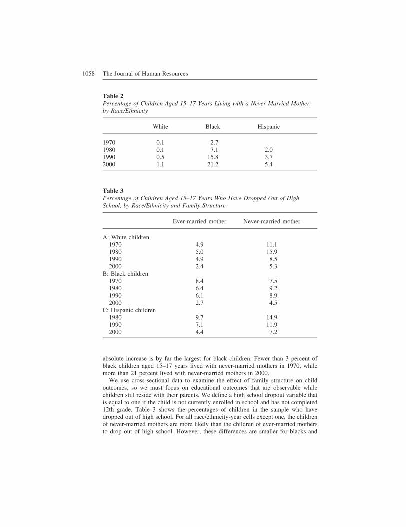
Table 2Percentage of Children Aged 15–17 Years Living with a Never-Married Mother,by Race/Ethnicity

White Black Hispanic

1970 0.1 2.71980 0.1 7.1 2.01990 0.5 15.8 3.72000 1.1 21.2 5.4

Table 3Percentage of Children Aged 15–17 Years Who Have Dropped Out of HighSchool, by Race/Ethnicity and Family Structure

Ever-married mother Never-married mother

A: White children1970 4.9 11.11980 5.0 15.91990 4.9 8.52000 2.4 5.3

B: Black children1970 8.4 7.51980 6.4 9.21990 6.1 8.92000 2.7 4.5

C: Hispanic children1980 9.7 14.91990 7.1 11.92000 4.4 7.2

absolute increase is by far the largest for black children. Fewer than 3 percent ofblack children aged 15–17 years lived with never-married mothers in 1970, whilemore than 21 percent lived with never-married mothers in 2000.

We use cross-sectional data to examine the effect of family structure on childoutcomes, so we must focus on educational outcomes that are observable whilechildren still reside with their parents. We define a high school dropout variable thatis equal to one if the child is not currently enrolled in school and has not completed12th grade. Table 3 shows the percentages of children in the sample who havedropped out of high school. For all race/ethnicity-year cells except one, the childrenof never-married mothers are more likely than the children of ever-married mothersto drop out of high school. However, these differences are smaller for blacks and


Hispanics. In general, there has been a secular decline (since 1980) in the proportionof teens dropping out of high school, which is captured in the year effects in ourmodels.

We create a number of control variables from the IPUMS data. Using informationfrom the mother’s record, we construct dummy variables for: mother has not finishedhigh school, has finished high school only, has finished only some college, and hasfinished at least four years of college. Table 4 shows that, compared with all othermothers, never-married mothers are nine percentage points less likely to have com-pleted four years of college, about as likely to have some college education, threepercentage points less likely to have completed only high school, and 12 percentagepoints more likely to have dropped out of high school. In addition to controlling forthe mother’s education, we calculate the age of the mother at time of the child’sbirth. Never-married mothers have their children at an average age of 22.8, whileother mothers have their children at an average age of 26.5. Never-married mothershave on average fewer children than those who have married—2.1 versus 2.8.

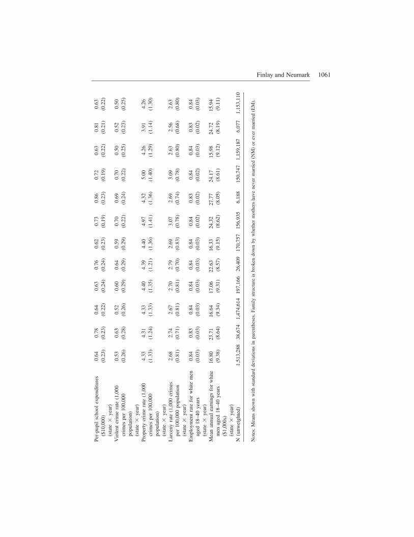
State-varying controls are in some cases taken from other sources. First, we in-clude per-pupil elementary- and secondary-school expenditures by state for the fiscalyears 1969–70, 1979–80, 1989–90, and 1999–2000.17 Second, we use three-yearmoving averages of the crime rates from the Federal Bureau of Investigation’s Uni-form Crime Reports, for violent crime and property crime (the two broadest crimecategories) as well as larceny, which is a subset of property crime involving neitherviolence nor fraud.18 Third, we estimate the employment rate and mean annualearnings of men aged 18–40 by state and year from the IPUMS. To avoid endog-enous effects of incarceration, we construct these statistics for white men.

We use state institutionalization rates as a proxy for state incarceration rates,following other work in this and related areas (for example, Butcher and Piehl 2007;Charles and Luoh 2010). Ideally, our incarceration rates would come from admin-istrative records from the Bureau of Justice Statistics (BJS). Unfortunately, the BJSdoes not publish data by state and race or ethnicity, and the data they can makeavailable with estimates by state and race or ethnicity are not considered reliable.Data from the decennial Censuses provide a suitable proxy, since they cover boththe institutionalized and noninstitutionalized populations. In addition, Census em-ployees use administrative records if institutionalized respondents are unable to fillout the Census forms, so the institutionalized population is well accounted for inthe IPUMS.

The institutionalization rate is defined as the proportion of respondents residingin institutional group quarters, including correctional facilities, mental institutions,and retirement facilities. Noninstitutional group quarters include military housingand college dormitories, and these individuals are excluded from the calculation ofinstitutionalization rates. Based on 1970 and 1980 data, in which institutional cate-gories are broken down so that incarceration in jails or prisons could be separatelyidentified, for younger men large shares of the population institutionalized were

17. These data come from the Digest of Education Statistics 2005 (http://nces.ed.gov/programs/digest/d05/tables/dt05_167.asp, accessed on March 17, 2007).18. The raw data come from the website of the Bureau of Justice Statistics (http://bjsdata.ojp.usdoj.gov/dataonline/Search/Crime/State/statebystatelist.cfm, accessed on May 20, 2007).


Tab

le4

Sele

cted

Des

crip

tive

Stat

isti

cs,

Chi

ldre

nA

ged

15–1

7Y

ears

Liv

ing

wit

hT

heir

Mot

hers

,by

Rac

e,E

thni

city

,an

dF

amil

ySt

ruct

ure

Bla

ckB

lack

Bla

ckH

ispa

nic

His

pani

cH

ispa

nic

Whi

teW

hite

Whi

teV

aria

ble

All

NM

EM

All

NM

EM

All

NM

EM

All

NM

EM

Nev

er-m

arri

edm

othe

r0.

020.

120.

040.

00

Bla

ck0.

140.

700.

12

His

pani

c0.

080.

150.

08

Chi

ldha

sdr

oppe

dou

tof

high

scho

ol0.

050.

070.

050.

060.

070.

060.

070.

090.

070.

040.

070.

04

Mot

her

did

not

finis

hhi

ghsc

hool

0.26

0.38

0.26

0.40

0.36

0.41

0.52

0.57

0.52

0.21

0.23

0.21

Mot

her

finis

hed

just

high

scho

ol0.

400.

370.

400.

340.

390.

330.

270.

260.

270.

430.

400.

43

Mot

her

finis

hed

som

eco

llege

0.21

0.21

0.21

0.19

0.21

0.19

0.16

0.14

0.16

0.22

0.27

0.22

Mot

her

finis

hed

colle

ge0.

130.

040.

130.

070.

040.

070.

060.

030.

060.

140.

090.

14

Mot

her’

sag

eat

birt

hof

child

26.4

022

.82

26.4

825

.33

22.4

325

.71

25.7

523

.81

25.8

326

.65

23.6

726

.67

(5.9

0)(5

.66)

(5.8

8)(6

.56)

(5.5

6)(6

.58)

(6.1

7)(5

.98)

(6.1

6)(5

.72)

(5.6

0)(5

.71)

Num

ber

ofsi

blin

gsin

hous

ehol

d2.

732.

072.

753.

072.

213.

182.

992.

203.

022.

651.

262.

65(2

.14)

(1.8

2)(2

.14)

(2.3

8)(1

.85)

(2.4

2)(2

.16)

(1.7

9)(2

.17)

(2.0

9)(1

.48)

(2.0

9)In

stitu

tiona

lizat

ion

rate

for

0.01

00.

045

0.01

00.

035

0.05

70.

033

0.01

90.

025

0.01

90.

005

0.01

00.

005

sam

e-ra

cem

en(s

tate

ofre

side

nce

�ra

ce�

year

�ag

egr

oup)

(0.0

17)

(0.0

35)

(0.0

15)

(0.0

31)

(0.0

34)

(0.0

29)

(0.0

14)

(0.0

15)

(0.0

14)

(0.0

05)

(0.0

05)

(0.0

05)


Per-

pupi

lsc

hool

expe

nditu

res

0.64

0.78

0.64

0.63

0.76

0.62

0.73

0.86

0.72

0.63

0.81

0.63

($10

,000

)(s

tate

�ye

ar)

(0.2

3)(0

.23)

(0.2

2)(0

.24)

(0.2

4)(0

.23)

(0.1

9)(0

.23)

(0.1

9)(0

.22)

(0.2

1)(0

.22)

Vio

lent

crim

era

te(1

,000

0.53

0.63

0.52

0.60

0.64

0.59

0.70

0.69

0.70

0.50

0.52

0.50

crim

espe

r10

0,00

0po

pula

tion)

(sta

te�

year

)

(0.2

6)(0

.28)

(0.2

6)(0

.29)

(0.2

9)(0

.29)

(0.2

2)(0

.24)

(0.2

2)(0

.25)

(0.2

3)(0

.25)

Prop

erty

crim

era

te(1

,000

4.33

4.31

4.33

4.40

4.39

4.40

4.97

4.32

5.00

4.26

3.91

4.26

crim

espe

r10

0,00

0po

pula

tion)

(sta

te�

year

)

(1.3

3)(1

.24)

(1.3

3)(1

.35)

(1.2

1)(1

.36)

(1.4

1)(1

.36)

(1.4

0)(1

.29)

(1.1

4)(1

.30)

Lar

ceny

rate

(1,0

00cr

imes

2.68

2.74

2.67

2.70

2.79

2.69

3.07

2.69

3.09

2.63

2.56

2.63

per

100,

000

popu

latio

n(s

tate

�ye

ar)

(0.8

1)(0

.71)

(0.8

1)(0

.81)

(0.7

0)(0

.83)

(0.7

8)(0

.74)

(0.7

8)(0

.80)

(0.6

8)(0

.80)

Em

ploy

men

tra

tefo

rw

hite

men

0.84

0.83

0.84

0.84

0.84

0.84

0.84

0.83

0.84

0.84

0.83

0.84

aged

18–4

0ye

ars

(sta

te�

year

)(0

.03)

(0.0

3)(0

.03)

(0.0

3)(0

.03)

(0.0

3)(0

.02)

(0.0

2)(0

.02)

(0.0

3)(0

.02)

(0.0

3)

Mea

nan

nual

earn

ings

for

whi

te16

.80

23.7

116

.64

17.0

622

.63

16.3

324

.32

27.7

724

.17

15.9

824

.72

15.9

4m

enag

ed18

–40

year

s($

1,00

0s)

(sta

te�

year

)

(9.3

8)(8

.64)

(9.3

4)(9

.31)

(8.5

7)(9

.15)

(8.6

2)(8

.05)

(8.6

1)(9

.12)

(8.1

9)(9

.11)

N(u

nwei

ghte

d)1,

513,

288

38,6

741,

474,

614

197,

166

26,4

0917

0,75

715

6,93

56,

188

150,

747

1,15

9,18

76,

077

1,15

3,11

0

Not

es:

Mea

nssh

own

with

stan

dard

devi

atio

nsin

pare

nthe

ses.

Fam

ilyst

ruct

ure

isbr

oken

dow

nby

whe

ther

mot

hers

have

neve

rm

arri

ed(N

M)

orev

erm

arri

ed(E

M).


clearly incarcerated (Butcher and Piehl 2007; Charles and Luoh 2010).19 Aggregatedata by race on incarceration based on the Census institutionalization definition isconsistent with information from the Bureau of Justice Statistics (Raphael 2006).Each child observation is assigned an institutionalization rate based on the mother’sage, child’s race or ethnicity, state of residence, and year. Mothers aged t years areassigned the institutionalization rate for the appropriate sample of men aged t tot�5 years. This age range was chosen based on the observed relationship betweenspousal ages in the United States (husbands are about two years older than wives)combined with the evidence that women in poor, urban communities are more likelyto marry older men (Vera, Berardo, and Berardo 1985).

Despite institutionalization capturing incarceration well, there are other sources oferror in measuring incarceration rates. Sampling error is more likely for minoritiesin small states because of small sample sizes, and sampling error is also more likelyin 1970 than in the other years because the sample is one-fifth the size of the 1980–2000 samples. In addition, there is a potential aggregation problem because incar-ceration rates are calculated at the state level (the level at which the analysis isdone), but they may have more local effects.20 However, since incarceration is notmeasured at the household level, there is no way to use Census data to constructmore geographically disaggregated measures of incarceration.

If marriage decisions are primarily made at young ages (like the late teens orearly 20s), then given that we are studying children aged 15–17, the lagged incar-ceration rate instrumental variable that we use is more appropriate. On the otherhand, research indicates that contemporaneous incarceration rates of older men arelikely to be important as well. Evidence shows that many first marriages are expe-rienced by men in their 30s. For example, based on 2002 data, the percentage ofblack men ever married rises from 46 percent at age 30 to 74 percent at age 40(Lichter and Graefe 2007).21 For Hispanics and nonblack non-Hispanics, the increaseis smaller by 18 to 20 percentage points over this age range (from 60 to 78 percentand 62 to 82 percent, respectively). Furthermore, for the lower-income populationof single women with children, qualitative evidence indicates that there is a normof childbearing first followed by a desire for marriage later. The delay arises bothbecause women want men to have established themselves financially and womenwant to have established themselves financially so that they can legitimately threaten

19. In our own calculations from the 1980 Census, we estimate the proportion of institutionalized menwho reside in a correctional facility by race, ethnicity, and single-year age group. For blacks and Hispanics,this proportion is higher than 80 percent at age 19 and above 75 percent at ages 30 and 40. By age 50,this proportion falls to 45 percent for blacks and 60 percent for Hispanics. This provides yet another reasonto prefer the lagged incarceration rate instrumental variable, as it is based on the more accurate institu-tionalization rates measured at younger ages. Nonetheless, as long as the across-state-and-year variation ininstitutionalization rates is driven by variation in incarceration rates, the rates for older men will still providevalid identifying information.20. There is a question as to whether the effective marriage market should be defined at the state level.Charles and Luoh (2010) use a state-level definition like we do. Brien (1997) explores the explanatorypower of marriage markets defined at the state versus local level, and finds that state-level definitions workbetter.21. Similarly, Lichter, Graefe, and Brown (2003) study 24–45 year-olds in the 1995 National Survey ofFamily Growth, and find that of those who have an out-of-wedlock child, 41 percent subsequently marry.


to leave marriages that, for this subpopulation, are often to men with drug-, crime-,or abuse-related problems with relatively low economic security (Edin 2000; Edinand Reed 2005). Indeed, many women reported that the ideal age for childbearingwas in a woman’s early 20s, while the ideal age for marriage was in the late 20s orearly 30s. Finally, the contemporaneous incarceration rate for older males may beappropriate given that women who give birth out of wedlock are more likely tomarry older men if they do marry (Qian, Lichter, and Mellott 2005).

Figure 1 shows histograms for incarceration rates for men aged 18–40 years acrossstates in 1980, 1990, and 2000. Incarceration rates for whites are low in all statesas of 2000. In contrast, incarceration rates in most states are much higher for His-panics, and more so for blacks. Moreover, for both minority groups incarcerationrates clearly increased over these decades. Figure 2 shows the histograms of changesin incarceration rates across states over the periods 1980–1990, 1990–2000, and1980–2000; the vertical axes show the number of states with changes in incarcerationrates in the indicated ranges.22 These histograms show dramatic increases in incar-ceration rates for minorities, especially in some states, with the greatest increasesbetween 1990 and 2000. Figures 1 and 2 indicate that the shares of blacks andHispanics potentially affected by changes in incarceration rates are substantial.23 Thisvariation is central to our identification strategy. Because of the absence of substan-tial changes for whites, coupled with low incarceration rates for them in general aswell as low never-married rates, we focus on blacks and Hispanics in our analysis.

There might be some concern that increases in incarceration have been concen-trated in particular geographic regions of the country. Figure 3 maps the changes inincarceration. States with no shading had the smallest increases in the incarcerationrate for black men aged 18–40 years (or even slight decreases). States with thedarkest shading had the greatest increases in these rates. The figure shows that stateswith small, medium, and large increases in black incarceration are represented in allmajor regions of the country.

Table 5 presents descriptive statistics on the percentage of children aged 15–17living with a never-married mother. The columns are broken down by whether theincarceration rate for men aged 18–40 years and the same race or ethnicity as thechild is less than the 25th percentile, between the 25th and 75th percentiles, orgreater than the 75th percentile. The percentiles are calculated for each year of thesample and also for the pooled sample—to reveal how variation in incarcerationrates is associated with the rate of never-married motherhood across states withineach year, and for the whole sample. Looking across the columns, the table providesrelatively clear evidence that in states and years with higher incarceration rates therates of never-married motherhood are higher for blacks and Hispanics, althoughthere are some exceptions, especially in the early years in the sample for blacks.For white women, however, this pattern is not apparent, and within years whitewomen appear to respond quite differently to higher male incarceration, as livingin a state with less incarceration is associated with lower rates of never-married

22. There are some extreme values generated by small cells, but since we use individual-level data, theseobservations have an inconsequential influence on the results.23. Any given increase in incarceration rates over a decade implies a considerably larger increase in theprobability that an individual was incarcerated at some point over that decade.


Figure 1Histogram of Incarceration Rates for Men Aged 18–40 Years, Across States, byRace and Ethnicity, 1980, 1990, 2000Note: The unit of observation for each histogram is the state.


Figure 2Histogram of Changes in Incarceration Rates for Men Aged 18–40 Years, AcrossStates, by Race and Ethnicity, from 1980 to 1990, 1990 to 2000, and 1980 to2000Note: The unit of observation for each histogram is the state.


Figure 3Changes in Incarceration Rates for Black Men Aged 18–40 Years from 1980 to2000, by StateNotes: No shading indicates a small change in the incarceration rate for black men (between -1 and �5.4percentage points). Light shading indicates a medium change (between �5.4 and �9 percentage points).Dark shading indicates a large change (between �9 and �22 percentage points). These cutoffs are ap-proximately tritiles of the distribution of changes by state. Rates from 1980 are used as a baseline for thedifferences because the 1970 data are relatively noisy.

motherhood; for this reason, as well, our analysis focuses on black and Hispanicchildren.24

VI. Results

A. Main results

We begin with estimates of the equations for never-married motherhood. Table 6reports estimates from probit regressions, in Columns 2 and 5 using the contem-

24. The regression analysis, based on age-specific incarceration rates, leads to a similar conclusion thatthe incarceration “experiment” does not work for whites. In the first-stage equation for never-marriedmotherhood, the effect of incarceration was much weaker for whites than for blacks or Hispanics, usinglinear probability or probit. For the probit estimation, the estimated effect of the preferred lagged incar-ceration rate was near zero and statistically insignificant.


Table 5Percentage of Children Aged 15–17 Years Living with a Never-Married Mother,by Race/Ethnicity, and by Percentile of Incarceration Rate for Men Aged 18–40Years

Percentile of state-year-race/ethnicityincarceration rate

25th 25th–75th 75th

A: White children1970 0.08 0.08 0.071980 0.19 0.12 0.111990 0.56 0.51 0.332000 1.30 1.19 0.88Pooled years 0.14 0.31 0.88

B: Black children1970 2.74 2.67 2.601980 7.64 7.06 6.551990 16.09 15.47 16.502000 19.69 20.60 24.33Pooled years 5.73 9.77 20.54

C: Hispanic children1980 1.05 1.45 4.691990 3.70 2.02 6.532000 4.97 4.02 9.10Pooled years 1.06 3.74 6.59

Notes: In the first four rows of each panel, percentiles are calculated separately for each race/ethnicity andyear. In the last row of each panel, percentiles are calculated for each race/ethnicity across all years.

poraneous incarceration rate, and in Columns 3 and 6 using the lagged incarcerationrate. For blacks, the estimated marginal effect of the current incarceration rate is0.528 (Column 2), and 0.184 (Column 3) for the lagged incarceration rate. Thecurrent rate is statistically significantly different from zero at the 1 percent level,and the lagged rate at the 10 percent level. For Hispanics, the estimated marginaleffect of the current rate is 0.221 (Column 5), and 0.167 (Column 6) for the laggedrate. The current rate is statistically significant at the 1 percent level and the laggedrate is statistically significant at the 5 percent level. To put these estimates in context,the approximate modal increases in incarceration rates over the 1980–2000 periodwere 0.07 for black men and 0.02 for Hispanic men. Thus, for blacks, for example,the probit estimates imply that the modal increase in contemporaneous incarcerationwould lead to a 3.7 percentage point increase in never-married motherhood, or a 52


Tab

le6

Pro

bit

Est

imat

esof

Mod

els

for

Nev

er-M

arri

edM

othe

rhoo

d,C

hild

ren

Age

d15

–17

Yea

rsL

ivin

gw

ith

The

irM

othe

rs,

byR

ace

and

Eth

nici

ty

Bla

ckB

lack

Bla

ckH

ispa

nic

His

pani

cH

ispa

nic

Inde

pend

ent

vari

able

s(1

)(2

)(3

)(4

)(5

)(6

)

Inca

rcer

atio

nra

te0.

528

0.22

1(s

tate

ofre

side

nce,

year

t)(0

.106

)(0

.085

)In

carc

erat

ion

rate

0.18

40.

167

(sta

teof

birt

h,ye

art-

10)

(0.1

05)

(0.0

73)

Fem

ale

(chi

ld)

0.00

070.

0006

0.00

160.

0020

0.00

200.

0016

(0.0

011)

(0.0

011)

(0.0

016)

(0.0

008)

(0.0

008)

(0.0

007)

Per-

pupi

led

ucat

iona

lex

pens

es($

1,00

0s)

0.07

40.

070

0.01

90.

001

�0.

004

�0.

000

(0.0

27)

(0.0

27)

(0.0

36)

(0.0

14)

(0.0

15)

(0.0

17)

Vio

lent

crim

era

te(1

,000

crim

es0.

032

0.01

20.

017

0.02

00.

015

0.02

2pe

r10

0,00

0po

pula

tion)

(0.0

23)

(0.0

23)

(0.0

21)

(0.0

07)

(0.0

08)

(0.0

08)

Prop

erty

crim

era

te(1

,000

crim

es0.

002

0.00

70.

017

0.00

80.

012

0.01

0pe

r10

0,00

0po

pula

tion)

(0.0

09)

(0.0

08)

(0.0

13)

(0.0

05)

(0.0

06)

(0.0

06)

Lar

ceny

rate

(1,0

00cr

imes

per

�0.

023

�0.

022

�0.

036

�0.

020

�0.

025

�0.

023

100,

000

popu

latio

n)(0

.013

)(0

.013

)(0

.020

)(0

.007

)(0

.008

)(0

.009

)E

mpl

oym

ent

rate

for

whi

tem

en0.

122

0.18

40.

442

0.02

60.

006

�0.

014

aged

18–4

0ye

ars

(0.1

26)

(0.1

17)

(0.1

40)

(0.0

51)

(0.0

52)

(0.0

64)

Mea

nea

rnin

gsfo

rw

hite

men

aged

�0.

0006

0.00

040.

0019

�0.

0003

0.00

000.

0003

18–4

0ye

ars

($1,

000s

)(0

.001

2)(0

.001

2)(0

.001

1)(0

.000

8)(0

.000

8)(0

.000

7)M

othe

ris

high

scho

olgr

adua

te�

0.04

3�

0.04

2�

0.05

9�

0.01

2�

0.01

2�

0.01

4(0

.002

)(0

.002

)(0

.002

)(0

.001

)(0

.001

)(0

.002

)


Mot

her

has

som

eco

llege

�0.

063

�0.

063

�0.

089

�0.

016

�0.

016

�0.

017

(0.0

02)

(0.0

02)

(0.0

02)

(0.0

01)

(0.0

01)

(0.0

01)

Mot

her

has

four

year

sof

colle

ge�

0.07

3�

0.07

3�

0.10

4�

0.02

2�

0.02

2�

0.02

2(0

.002

)(0

.002

)(0

.002

)(0

.001

)(0

.001

)(0

.001

)A

geof

mot

her

atbi

rth

ofch

ild�

0.00

72�

0.00

60�

0.00

97�

0.00

18�

0.00

16�

0.00

19(0

.000

2)(0

.000

3)(0

.000

3)(0

.000

1)(0

.000

1)(0

.000

1)N

umbe

rof

sibl

ings

inho

use

�0.

013

�0.

013

�0.

016

�0.

007

�0.

007

�0.

007

(0.0

01)

(0.0

01)

(0.0

01)

(0.0

01)

(0.0

01)

(0.0

01)

Obs

erva

tions

197,

085

196,

763

178,

679

151,

859

151,

736

111,

299

Pseu

doR

20.

150.

150.

120.

100.

100.

12M

ean

ofde

pend

ent

vari

able

0.12

0.12

0.14

0.04

0.04

0.04

Not

es:

The

inca

rcer

atio

nra

teva

riab

leis

defin

edba

sed

onth

ew

oman

’sag

e,ra

ce/e

thni

city

,st

ate,

and

year

.For

wom

enof

age

ain

year

t,th

ein

carc

erat

ion

rate

isde

fined

for

men

aged

ato

a�

5(a

ndag

ea

–10

toag

ea

–5

for

wom

enof

age

a–

10in

year

t�

10).

Eac

hsp

ecifi

catio

nin

clud

esch

ildag

eef

fect

s,st

ate

effe

cts,

year

effe

cts,

and

child

age-

year

effe

cts.

Est

imat

esco

me

from

prob

itsp

ecifi

catio

n;ta

ble

repo

rts

mar

gina

lef

fect

sth

atar

eev

alua

ted

atth

em

eans

ofea

chsp

ecifi

catio

n’s

resp

ectiv

esa

mpl

e.H

eter

osce

dast

icity

-rob

ust

stan

dard

erro

rs,

clus

tere

dat

the

stat

ele

vel,

are

inpa

rent

hese

s.A

lles

timat

esar

ew

eigh

ted

byIP

UM

Spe

rson

wei

ghts

.D

ata

from

1970

are

not

used

inth

ees

timat

ion

for

His

pani

cs.


percent increase over the rate of 7.1 percent in 1980 (Table 2); the correspondingnumbers for Hispanics are 0.4 percentage point and 22 percent.25

Table 7 reports our first set of estimates of the models for whether a child hasdropped out of high school. OLS estimates that do not account for endogenousselection (Columns 1 and 4) indicate that black and Hispanic children are morelikely, on average, to have dropped out of high school if they live with a never-married mother. In particular, blacks and Hispanics living with never-married moth-ers are 1.5 and 3.2 percentage points more likely to have dropped out of high school,respectively. Given mean dropout rates at these ages of 6 percent for blacks and 7percent for Hispanics, these are large effects.

The two-stage instrumental variables estimates that account for nonrandom selec-tion into never-married motherhood are reported in Columns 2, 3, 5, and 6. Forblacks, the estimated effects of never-married motherhood on whether a child hasdropped out of high school become negative, indicating a lower likelihood of dropoutassociated with never-married motherhood (0.3 to 0.9 percentage point), althoughthe estimates are fairly small and statistically insignificant. For Hispanics, as well,the estimated effects of never-married motherhood on whether a child has droppedout of high school become negative, but in this case the estimates are larger. Hispanicchildren of mothers who are affected by variation in the incarceration of men areestimated to be between three and 8.2 percentage points less likely to drop out ofhigh school. The latter estimate, which is based on the lagged incarceration rateinstrumental variable, is statistically significant. The Anderson-Rubin test of the nullhypothesis that the coefficient on never-married motherhood is equal to zero providesvery similar inference to an analogous Wald test (for example, p-values of 0.485and 0.031 for Hispanics), which indicates that the statistical inferences for the two-stage instrumental variables estimates are valid.

Table 8 relaxes the specification of the effects of incarceration by adding poly-nomials of incarceration rates into the model for never-married motherhood. Theestimated probit marginal effects (not shown) indicate that the effects of incarcera-tion rates on never-married motherhood are stronger at higher incarceration rates.Moreover, for both blacks and Hispanics the �2-statistic for the joint significance ofthe incarceration rate in the never-married motherhood probit is greater in the non-linear models than in the corresponding specification in Table 7. However, the sec-ond-stage results when nonlinear effects of the incarceration rate are allowed inTable 8 are very similar to those in Table 7.

The estimates of the effect of never-married motherhood on whether children havedropped out of high school have two implications. First, they suggest that unob-servable characteristics drive the selection into never-married motherhood and thenegative school outcomes of the children of never-married mothers, for those womenwhose marriage decisions are affected by variation in incarceration rates. And sec-

25. We also estimated these models for three separate education groups: high school dropouts, high schoolgraduates, and any college. For blacks and Hispanics the estimated effects of incarceration decline sharplyas education increases, and are never significant for the two higher education groups. This bolsters thelocal average treatment effect interpretation of the estimates as identifying the effects for less-educatedwomen whose marriage prospects are more strongly affected by variation in incarceration rates.


ond, they suggest that, for Hispanic children, never-married motherhood may actu-ally reduce the likelihood of dropping out.

B. Identification and robustness checks

A potential concern regarding the two-stage instrumental variables estimation is thatthe nonlinear functions of the control variables in the fitted probability of never-married motherhood, rather than the variation in incarceration rates, serve to identifythe effect of never-married motherhood. To avoid relying on this type of identifyinginformation, we can estimate the model using linear probability specifications andtwo-stage least squares. This approach may yield relatively imprecise estimates inour case, given that the never-married motherhood rate is quite low, especially earlyin the sample period; as a result, linear probability estimates of the first stage leadto many negative fitted values, which may result in a much weaker first stage as thevariation near and below zero in the estimates of the first stage estimated as a linearprobability model are not associated with actual variation in never-married status.26

Table 9 reports two-stage least squares results using polynomials of the incarcerationrate instruments. There is a loss of precision relative to the two-stage instrumentalvariables models. For blacks and Hispanics, the standard errors of the estimatedeffects of never-married motherhood are roughly two to four times as large. Theresulting estimates are never positive and significant, in contrast to the OLS estimatesthat indicate an adverse effect of never-married motherhood. However, the sign ofthe instrumental variables estimate of the effect of never-married motherhood is inthis case sensitive to using current versus lagged incarceration rates as instruments.In particular, the estimated effect is consistently negative (for blacks and Hispanics)when the lagged incarceration rates are used as instruments. But the results highlightthat drawing stronger conclusions from the data hinges on using the two-stage in-strumental variables estimation strategy.

A second identification-related issue, discussed earlier, is that incarceration ratesmay have direct effects on child outcomes. The most plausible scenario is that in-carceration rates of older men (or lagged incarceration rates of younger men) arecorrelated with contemporaneous variation in incarceration rates of younger men.Incarceration of younger men could directly affect the costs and benefits of alter-native decisions made by teenagers and hence their decisions to drop out of highschool.27 In this case, the exclusion restriction underlying the instrumental variablesestimation is invalid, and our estimates may instead reflect the direct effect of in-carceration, albeit still suggesting that higher incarceration leads to better outcomesfor children.

To address this concern that the inclusion of crime rates and other controls arenot sufficient to prevent the violation of the exclusion restriction, we calculate theincarceration rate for same-race/ethnicity men aged 18–24 years living in the same

26. See Angrist (1991) and Bhattacharya, Goldman, and McCaffrey (2006) for discussion of these andrelated issues for the two-equation linear probability model.27. As an example, a referee suggested that higher incarceration of youths may be associated with thebreak-up of gangs, and consequently higher enrollment of those prone to gang membership, who may bemore likely to be the children of never-married mothers.


Tab

le7

OL

San

dT

wo-

Stag

eIn

stru

men

tal

Var

iabl

esR

egre

ssio

nE

stim

ates

ofM

odel

sfo

rW

heth

erC

hild

Has

Dro

pped

Out

ofH

igh

Scho

ol,

Chi

ldre

nA

ged

15–1

7Y

ears

Liv

ing

wit

hT

heir

Mot

hers

,by

Rac

ean

dE

thni

city

Bla

ckB

lack

Bla

ckH

ispa

nic

His

pani

cH

ispa

nic

Inde

pend

ent

vari

able

sO

LS

(1)

2SIV

(2)

2SIV

(3)

OL

S(4

)2S

IV(5

)2S

IV(6

)

End

ogen

ous

cova

riat

esM

othe

rne

ver

mar

ried

0.01

5�

0.00

3�

0.00

90.

032

�0.

030

�0.

082

(0.0

02)

(0.0

16)

(0.0

17)

(0.0

04)

(0.0

44)

(0.0

39)

And

erso

n-R

ubin

p-va

lue

0.86

30.

605

0.48

50.

031

Oth

erco

ntro

lsFe

mal

e(c

hild

)�

0.00

51�

0.00

51�

0.00

57�

0.00

51�

0.00

76�

0.00

52(0

.001

5)(0

.001

5)(0

.001

5)(0

.001

5)(0

.001

4)(0

.001

5)Pe

r-pu

pil

educ

.ex

p.($

1,00

0s)

�0.

001

0.00

4�

0.00

1�

0.00

10.

073

0.07

4(0

.017

)(0

.017

)(0

.018

)(0

.017

)(0

.022

)(0

.026

)V

iole

ntcr

ime

rate

0.03

40.

034

0.03

60.

034

0.00

20.

002

(1,0

00cr

imes

per

100,

000

popu

latio

n)(0

.012

)(0

.012

)(0

.013

)(0

.012

)(0

.012

)(0

.013

)Pr

oper

tycr

ime

rate

�0.

001

�0.

001

0.00

1�

0.00

10.

009

0.00

8(1

,000

crim

espe

r10

0,00

0po

pula

tion)

(0.0

06)

(0.0

06)

(0.0

06)

(0.0

06)

(0.0

06)

(0.0

07)

Lar

ceny

rate

�0.

010

�0.

010

�0.

013

�0.

010

�0.

011

�0.

016

(1,0

00cr

imes

per

100,

000

popu

latio

n)(0

.009

)(0

.009

)(0

.010

)(0

.009

)(0

.010

)(0

.012

)E

mpl

oym

ent

rate

for

whi

tem

enag

ed0.

161

0.16

00.

151

0.16

10.

434

0.18

218

–40

year

s(0

.072

)(0

.072

)(0

.076

)(0

.072

)(0

.094

)(0

.106

)M

ean

earn

ings

for

whi

tem

enag

ed18

–40

�0.

0003

�0.

0004

�0.

0003

�0.

0003

�0.

0005

�0.

0000

year

s($

1,00

0s)

(0.0

006)

(0.0

006)

(0.0

006)

(0.0

006)

(0.0

008)

(0.0

009)


Mot

her

ishi

ghsc

hool

grad

uate

�0.

041

�0.

042

�0.

043

�0.

041

�0.

047

�0.

039

(0.0

02)

(0.0

02)

(0.0

02)

(0.0

02)

(0.0

02)

(0.0

02)

Mot

her

has

som

eco

llege

�0.

053

�0.

055

�0.

056

�0.

053

�0.

056

�0.

046

(0.0

02)

(0.0

03)

(0.0

03)

(0.0

02)

(0.0

02)

(0.0

02)

Mot

her

has

four

year

sof

colle

ge�

0.06

3�

0.06

6�

0.06

8�

0.06

3�

0.06

7�

0.05

9(0

.002

)(0

.003

)(0

.003

)(0

.002

)(0

.003

)(0

.003

)A

geof

mot

her

atbi

rth

ofch

ild0.

0000

�0.

0001

�0.

0001

0.00

00�

0.00

04�

0.00

07(0

.000

1)(0

.000

2)(0

.000

2)(0

.000

1)(0

.000

2)(0

.000

2)N

umbe

rof

sibl

ings

inho

use

0.00

080.

0006

0.00

050.

0008

0.00

06�

0.00

06(0

.000

4)(0

.000

5)(0

.000

5)(0

.000

4)(0

.000

5)(0

.000

5)Fi

rst

stag

eIn

stru

men

tal

vari

able

s:In

carc

erat

ion

rate

(sta

teof

resi

denc

e,ye

art)

XX

Inca

rcer

atio

nra

te(s

tate

ofbi

rth,

year

t�10

)X

XPr

edic

ted

NM

1.13

91.

208

1.05

21.

158

(0.0

21)

(0.0

22)

(0.0

54)

(0.0

60)

F-s

tatis

ticfo

rin

stru

men

tal

vari

able

2,88

8.15

3,07

8.73

374.

6537

7.54

�2 -s

tatis

ticfo

rin

carc

erat

ion

rate

inpr

obit

76.2

38.

1216

.83

17.1

5O

bser

vatio

ns19

7,12

919

6,76

218

9,73

515

2,07

315

1,73

611

1,27

8R

20.

030.

04M

ean

ofde

pend

ent

vari

able

0.06

0.06

0.06

0.07

0.07

0.06

Not

es:

See

note

sto

Tab

le6

for

the

defin

ition

ofth

ein

carc

erat

ion

rate

s.E

ach

spec

ifica

tion

incl

udes

child

age

effe

cts,

stat

eef

fect

s,ye

aref

fect

s,an

dch

ildag

e-ye

aref

fect

s.H

eter

osce

dast

icity

-rob

ust

stan

dard

erro

rs,

clus

tere

dat

the

stat

ele

vel,

are

inpa

rent

hese

s.“2

SIV

”is

the

two-

step

inst

rum

enta

lvar

iabl

espr

oced

ure

desc

ribe

din

Woo

ldri

dge

(200

2,p.

623)

.A

lles

timat

esar

ew

eigh

ted

byIP

UM

Spe

rson

wei

ghts

.D

ata

from

1970

are

not

used

inth

ees

timat

ion

for

His

pani

cs.


Tab

le8

Tw

o-St

age

Inst

rum

enta

lV

aria

bles

Reg

ress

ion

Est

imat

esof

Mod

els

for

Whe

ther

Chi

ldH

asD

ropp

edO

utof

Hig

hSc

hool

,w

ith

Inca

rcer

atio

n-ra

teP

olyn

omia

lsin

the

Fir

stSt

age,

Chi

ldre

nA

ged

15–1

7Y

ears

Liv

ing

wit

hT

heir

Mot

hers

,by

Rac

ean

dE

thni

city

Bla

ckB

lack

Bla

ckB

lack

His

pani

cH

ispa

nic

His

pani

cH

ispa

nic

Inde

pend

ent

vari

able

s(1

)(2

)(3

)(4

)(5

)(6

)(7

)(8

)

End

ogen

ous

cova

riat

esM

othe

rne

ver

mar

ried

�0.

002

�0.

001

�0.

009

�0.

008

�0.

029

�0.

019

�0.

083

�0.

083

(0.0

16)

(0.0

16)

(0.0

17)

(0.0

17)

(0.0

44)

(0.0

43)

(0.0

38)

(0.0

37)

And

erso

n-R

ubin

p-va

lue

0.88

40.

964

0.60

10.

623

0.50

00.

656

0.02

80.

025

Oth

erco

ntro

lsFe

mal

e(c

hild

)�

0.00

5�

0.00

5�

0.00

6�

0.00

6�

0.00

8�

0.00

8�

0.00

5�

0.00

5(0

.001

)(0

.001

)(0

.001

)(0

.001

)(0

.001

)(0

.001

)(0

.001

)(0

.001

)Pe

r-pu

pil

educ

atio

nal

expe

nses

($1,

000s

)0.

004

0.00

4�

0.00

1�

0.00

10.

073

0.07

30.

074

0.07

4(0

.017

)(0

.017

)(0

.018

)(0

.018

)(0

.022

)(0

.022

)(0

.026

)(0

.026

)V

iole

ntcr

ime

rate

0.03

40.

034

0.03

60.

036

0.00

20.

003

0.00

20.

002

(1,0

00cr

imes

per

100,

000

popu

latio

n)(0

.012

)(0

.012

)(0

.013

)(0

.013

)(0

.012

)(0

.012

)(0

.013

)(0

.013

)Pr

oper

tycr

ime

rate

�0.

001

�0.

001

0.00

10.

001

0.00

90.

009

0.00

80.

008

(1,0

00cr

imes

per

100,

000

popu

latio

n)(0

.006

)(0

.006

)(0

.006

)(0

.006

)(0

.006

)(0

.006

)(0

.007

)(0

.007

)L

arce

nyra

te�

0.01

0�

0.01

0�

0.01

3�

0.01

3�

0.01

1�

0.01

1�

0.01

6�

0.01

6(1

,000

crim

espe

r10

0,00

0po

pula

tion)

(0.0

09)

(0.0

09)

(0.0

10)

(0.0

10)

(0.0

10)

(0.0

10)

(0.0

12)

(0.0

12)

Em

ploy

men

tra

tefo

rw

hite

men

aged

0.16

00.

160

0.15

10.

151

0.43

40.

430

0.18

20.

182

18–4

0ye

ars

(0.0

72)

(0.0

72)

(0.0

76)

(0.0

76)

(0.0

94)

(0.0

94)

(0.1

06)

(0.1

06)

Mea

nea

rnin

gsfo

rw

hite

men

aged

�0.

0004

�0.

0004

�0.

0003

�0.

0003

�0.

0005

�0.

0006

�0.

000

�0.

0000

18–4

0ye

ars

($1,

000s

)(0

.000

6)(0

.000

6)(0

.000

6)(0

.000

6)(0

.000

8)(0

.000

8)(0

.001

)(0

.000

9)M

othe

ris

high

scho

olgr

adua

te�

0.04

2�

0.04

2�

0.04

3�

0.04

3�

0.04

7�

0.04

6�

0.03

9�

0.03

9(0

.002

)(0

.002

)(0

.002

)(0

.002

)(0

.002

)(0

.002

)(0

.002

)(0

.002

)M

othe

rha

sso

me

colle

ge�

0.05

5�

0.05

4�

0.05

6�

0.05

6�

0.05

5�

0.05

5�

0.04

6�

0.04

6(0

.003

)(0

.003

)(0

.003

)(0

.003

)(0

.002

)(0

.002

)(0

.002

)(0

.002

)


Mot

her

has

four

year

sof

colle

ge�

0.06

6�

0.06

6�

0.06

8�

0.06

8�

0.06

7�

0.06

6�

0.05

9�

0.05

9(0

.003

)(0

.003

)(0

.003

)(0

.003

)(0

.003

)(0

.003

)(0

.003

)(0

.003

)A

geof

mot

her

atbi

rth

ofch

ild�

0.00

01�

0.00

01�

0.00

01�

0.00

01�

0.00

03�

0.00

03�

0.00

07�

0.00

07(0

.000

2)(0

.000

2)(0

.000

2)(0

.000

2)(0

.000

2)(0

.000

2)(0

.000

2)(0

.000

2)N

umbe

rof

sibl

ings

inho

use

0.00

060.

0006

0.00

050.

0005

0.00

070.

0007

�0.

0006

�0.

0006

(0.0

005)

(0.0

005)

(0.0

005)

(0.0

005)

(0.0

005)

(0.0

005)

(0.0

005)

(0.0

005)

Firs

tst

age

Inst

rum

enta

lva

riab

les:

Inca

rcer

atio

nra

te(s

tate

ofre

side

nce,

year

t)X

XX

X

Inca

rcer

atio

nra

tesq

uare

d(s

tate

ofre

side

nce,

year

t)X

XX

X

Inca

rcer

atio

nra

tecu

bed

(sta

teof

resi

denc

e,ye

art)

XX

Inca

rcer

atio

nra

te(s

tate

ofbi

rth,

year

t�10

)X

XX

X

Inca

rcer

atio

nra

tesq

uare

d(s

tate

ofbi

rth,

year

t�10

)X

XX

X

Inca

rcer

atio

nra

tecu

bed

(sta

teof

birt

h,ye

art�

10)

XX

Pred

icte

dN

M1.

143

1.11

71.

207

1.20

11.

053

1.02

61.

162

1.11

7(0

.021

)(0

.021

)(0

.022

)(0

.022

)(0

.054

)(0

.054

)(0

.059

)(0

.058

)F

-sta

tistic

for

inst

rum

enta

lva

riab

le29

11.2

629

12.9

330

73.4

230

68.3

637

7.93

367.

2638

3.61

376.

56�

2 -sta

tistic

for

inca

rcer

atio

nra

teva

riab

les

inpr

obit

76.4

112

8.01

8.63

12.6

117

.12

29.5

217

.14

41.1

7

Obs

erva

tions

196,

762

196,

762

189,

735

189,

735

151,

736

151,

736

111,

278

111,

278

Mea

nof

depe

nden

tva

riab

le0.

060.

060.

060.

060.

070.

070.

060.

06

Not

es:

See

note

sto

Tab

le7.


Tab

le9

Tw

o-St

age

Lea

stSq

uare

sR

egre

ssio

nE

stim

ates

ofM

odel

sfo

rW

heth

erC

hild

Has

Dro

pped

Out

ofH

igh

Scho

ol,

Chi

ldre

nA

ged

15–

17Y

ears

Liv

ing

wit

hT

heir

Mot

hers

,by

Rac

ean

dE

thni

city

Bla

ckB

lack

Bla

ckB

lack

His

pani

cH

ispa

nic

His

pani

cH

ispa

nic

Inde

pend

ent

vari

able

s(1

)(2

)(3

)(4

)(5

)(6

)(7

)(8

)

End

ogen

ous

cova

riat

esM

othe

rne

ver

mar

ried

0.01

10.

011

�0.

089

�0.

048

�0.

162

0.05

2�

0.02

6�

0.05

7(0

.034

)(0

.031

)(0

.055

)(0

.048

)(0

.169

)(0

.114

)(0

.142

)(0

.133

)A

nder

son-

Rub

inp-

valu

e0.

944

0.14

00.

241

0.24

10.

556

0.10

00.

570

0.75

3O

ther

cont

rols

Fem

ale

(chi

ld)

�0.

005

�0.

005

�0.

006

�0.

006

�0.

007

�0.

008

�0.

005

�0.

005

(0.0

01)

(0.0

01)

(0.0

02)

(0.0

02)

(0.0

01)

(0.0

01)

(0.0

02)

(0.0

02)

Per-

pupi

led

ucat

iona

lex

pens

es($

1,00

0s)

0.00

10.

001

0.01

40.

006

0.08

00.

071

0.07

60.

077

(0.0

18)

(0.0

18)

(0.0

21)

(0.0

20)

(0.0

23)

(0.0

22)

(0.0

26)

(0.0

26)

Vio

lent

crim

era

te0.

034

0.03

40.

037

0.03

70.

001

0.00

40.

005

0.00

3(1

,000

crim

espe

r10

0,00

0po

pula

tion)

(0.0

12)

(0.0

12)

(0.0

13)

(0.0

13)

(0.0

12)

(0.0

12)

(0.0

14)

(0.0

14)

Prop

erty

crim

era

te�

0.00

1�

0.00

10.

001

0.00

10.

011

0.00

90.

008

0.00

8(1

,000

crim

espe

r10

0,00

0po

pula

tion)

(0.0

06)

(0.0

06)

(0.0

06)

(0.0

06)

(0.0

06)

(0.0

06)

(0.0

07)

(0.0

07)

Lar

ceny

rate

�0.

010

�0.

010

�0.

015

�0.

014

�0.

013

�0.

010

�0.

016

�0.

016

(1,0

00cr

imes

per

100,

000

popu

latio

n)(0

.009

)(0

.009

)(0

.010

)(0

.010

)(0

.011

)(0

.010

)(0

.012

)(0

.012

)

Em

ploy

men

tra

tefo

rw

hite

men

0.15

80.

158

0.17

30.

163

0.47

30.

403

0.14

30.

157

aged

18–4

0ye

ars

(0.0

72)

(0.0

72)

(0.0

76)

(0.0

76)

(0.1

10)

(0.1

00)

(0.1

24)

(0.1

23)

Mea

nea

rnin

gsfo

rw

hite

men

aged

�0.

0004

�0.

0004

�0.

0005

�0.

0004

�0.

0003

�0.

0007

�0.

0003

�0.

0002

18–4

0ye

ars

($1,

000s

)(0

.000

6)(0

.000

6)(0

.000

6)(0

.000

6)(0

.000

8)(0

.000

8)(0

.001

0)(0

.001

0)M

othe

ris

high

scho

olgr

adua

te�

0.04

1�

0.04

1�

0.04

7�

0.04

5�

0.04

9�

0.04

5�

0.03

8�

0.03

8(0

.003

)(0

.002

)(0

.004

)(0

.003

)(0

.003

)(0

.003

)(0

.003

)(0

.003

)


Mot

her

has

som

eco

llege

�0.

053

�0.

053

�0.

065

�0.

060

�0.

059

�0.

054

�0.

045

�0.

045

(0.0

04)

(0.0

04)

(0.0

06)

(0.0

05)

(0.0

04)

(0.0

03)

(0.0

04)

(0.0

04)

Mot

her

has

four

year

sof

colle

ge�

0.06

4�

0.06

4�

0.07

9�

0.07

3�

0.07

2�

0.06

3�

0.05

7�

0.05

8(0

.005

)(0

.005

)(0

.008

)(0

.007

)(0

.007

)(0

.005

)(0

.007

)(0

.006

)A

geof

mot

her

atbi

rth

ofch

ild0.

0000

0.00

00�

0.00

08�

0.00

04�

0.00

06�

0.00

02�

0.00

05�

0.00

06(0

.000

3)(0

.000

3)(0

.000

5)(0

.000

4)(0

.000

4)(0

.000

3)(0

.000

4)(0

.000

4)N

umbe

rof

sibl

ings

inho

use

0.00

070.

0007

�0.

0005

0.00

00�

0.00

030.

0013

�0.

0002

�0.

0004

(0.0

006)

(0.0

006)

(0.0

008)

(0.0

007)

(0.0

013)

(0.0

009)

(0.0

010)

(0.0

010)

Firs

tst

age

Inca

rcer

atio

nra

te1.

785

1.19

90.

730

�0.

728

(sta

teof

resi

denc

e,ye

art)

(0.0

93)

(0.1

75)

(0.1

32)

(0.2

60)

Inca

rcer

atio

nra

tesq

uare

d�

1.18

83.

401

�1.

559

32.1

22(s

tate

ofre

side

nce,

year

t)(0

.404

)(1

.325

)(1

.118

)(5

.648

)In

carc

erat

ion

rate

cube

d�

4.83

2�

169.

284

(sta

teof

resi

denc

e,ye

art)

(1.2

53)

(27.

117)

Inca

rcer

atio

nra

te�

0.01

3�

0.89

50.

814

0.35

7(s

tate

ofbi

rth,

year

t�10

)(0

.147

)(0

.185

)(0

.113

)(0

.176

)In

carc

erat

ion

rate

squa

red

5.23

720

.116

�2.

423

4.47

5(s

tate

ofbi

rth,

year

t�10

)(1

.223

)(3

.005

)(0

.475

)(2

.230

)In

carc

erat

ion

rate

cube

d�

63.5

83�

19.2

10(s

tate

ofbi

rth,

year

t�10

)(1

4.08

4)(5

.904

)F

-sta

tistic

for

inst

rum

enta

lva

riab

le29

6.93

195.

8559

.38

59.2

530

.95

26.0

027

.85

19.9

3O

bser

vatio

ns19

6,80

519

6,80

518

9,77

318

9,77

315

1,94

815

1,94

811

1,48

211

1,48

2M

ean

ofde

pend

ent

vari

able

0.06

0.06

0.06

0.06

0.07

0.07

0.06

0.06

Not

es:

See

note

sto

Tab

le7.


state as the child and add this as a control. These results are reported in Table 10.In Columns 1 and 6, we show OLS estimates comparable to the baseline estimationsin Table 7 but with the incarceration rate for men aged 18–24 years used as anadditional control. For blacks and Hispanics, there is essentially no change in theestimate of the coefficient on never-married motherhood. We use the contempora-neous incarceration rate as an instrument in the two-stage instrumental variablesmodel in Columns 2 and 7, and the lagged rate in Columns 3 and 8. In Columns 5and 10, we use both. (Columns 4 and 9 use both rates as instruments and leave outthe younger incarceration rate control, for comparison.) The estimates from thesemodels, which should be more robust to the exclusion restriction, all parallel theestimates from the baseline models. For blacks, the rates are all very close to zeroand statistically insignificant; all point estimates are negative. For Hispanics, as longas the lagged incarceration rate is used as an instrumental variable, never-marriedmotherhood is associated with a seven to eight percentage point reduction in theprobability of high school dropout, significant at the 5 or 10 percent level. Giventhat these specifications all require variation in incarceration rates for younger menthat is independent of variation in incarceration rates for potential spouses of themother, the evidence in Table 10 bolsters our conclusions by showing that our resultsare not confounded by a violation of the exclusion restriction stemming from a directeffect of the incarceration of younger men on teen outcomes.28

Finally, Table 11 presents a series of additional analyses and robustness checks.We begin by considering a couple of measurement issues. First, some prisoners areincarcerated outside of the state in which they previously resided. In that case, themeasured incarceration rate in a state may inaccurately capture the extent to whichmen have been removed from the marriage market. To more accurately capture howincarceration might affect the sex ratio, the estimates in Panel B are based on in-carceration rates calculated only for men who currently reside in the same state theydid five years before the Census. The two-stage instrumental variables estimates aresimilar to our baseline estimates.

Second, given the massive increase in adult incarceration, it is not surprising thatthere has been some increase in youth institutionalization.29 Institutionalized youthsare not in our sample because their family structures cannot be identified from theCensus data. If teen institutionalization is positive correlated with being raised by anever-married mother (owing in part to higher incarceration rates of men) and withdropping out of high school, both of which seem plausible, then our instrumentalvariables strategy may put more weight on the best performing children of never-

28. We also experimented with adding the instrumental variable based on the current incarceration rate asa control variable, instrumenting with the lagged incarceration rate only, to address the related but differentquestion about the direct effects of removing fathers to prison. For blacks, the predictive power of thelagged instrument in the first-stage probit using this specification was very low (the �2 statistic was only0.02), whereas for Hispanics it was higher (4.33, significant at the 5 percent level); this is reflected alsoin Table 6, where, for blacks, the current incarceration rate is a stronger predictor of never-married moth-erhood. Thus, only the instrumental variables estimation for Hispanics is relevant, and yielded evidencesimilar to that reported above, with an estimated coefficient (standard error) of never-married motherhoodof �0.078 (0.044).29. For black children aged 15–17, the institutionalization rate increased from 0.3 percent in 1970 to 2.2percent in 2000. For Hispanics, the rate increased from 0.08 percent in 1980 to 1.1 percent in 2000.


married mothers. To attempt to account for this, we estimated models for a sampleincluding institutionalized children. We classified all of these children as havingnever-married mothers, and imputed to their “mothers” the associated maternal con-trols for never-married mothers in the same state, year, and race/ethnic group. Asreported in Panel C, in most cases the estimates become more positive, consistentwith the possibility that our estimates are biased toward finding that never-marriedmotherhood reduces high school dropout. However, all of the estimates remain neg-ative, and the estimate for Hispanics remains statistically significant when the laggedincarceration rate is used as an instrument. Since this approach in a sense assumesthe worst—that all institutionalized children have never-married mothers—it nodoubt overstates the extent to which our estimates might be biased by the exclusionof institutionalized children. The findings therefore establish that youth institution-alization is not driving our results.

Finally, changes in other policies that affect schooling decisions may be correlatedwith changes in incarceration rates, biasing the instrumental variables estimates. Twopolicies of particular concern are compulsory schooling and minimum wage laws;minimum wages have been shown to reduce high school attendance among teenagers(for example, Neumark and Wascher 2003) and compulsory schooling laws to in-crease it (for example, Acemoglu and Angrist 2000). More generally, there may bechanges in nonschool opportunities that are contemporaneous with changes in in-carceration rates. In Panel D of Table 11 we present estimates of models in whichwe control for the state minimum wage, whether a child was covered by a compul-sory schooling law, and the employment rate for white 15–17 year-olds.30 The es-timates for both blacks and Hispanics are almost identical to those from the baselinespecifications.31

Summing up, none of the two-stage instrumental variables estimates point to evi-dence of a beneficial effect of never-married motherhood in reducing teen dropout,in contrast to OLS estimates that do not account for endogenous selection into never-married motherhood. For blacks, the sign of the instrumental variables estimatechanges across specifications, but is generally negative, always very small, and neverstatistically significant. For Hispanics, the sign of the instrumental variables estimatealways indicates that never-married motherhood reduces the likelihood that childrendrop out of high school, and the estimates are often statistically significant. Theseconclusions are robust to a battery of specifications intended to gauge the strengthof the evidence and the validity of the identification strategy.

30. Compulsory schooling laws come from various editions of the Digest of Education Statistics. Recordsare not available for every year, so we use the closest available listing of compulsory schooling laws: 1972laws for 1970, 1978 laws for 1980, 1989 laws for 1990, and 2000 laws for 2000. A child is coded ascovered by a compulsory schooling law if the child’s age is less than the maximum required age ofcompulsory schooling in a particular state and year. The minimum wage variable is the maximum of thestate and federal minimum wages in 1970, 1980, 1990, and 2000, adjusted to 1983 dollars using the All-Urban series of the Consumer Price Index.31. Although not reported in the table, the point estimates confirm earlier research, with higher minimumwages increasing the likelihood of dropping out (significant for blacks) and higher compulsory schoolingages lowering it (significant for Hispanics).


Tab

le10

Reg

ress

ion

Est

imat

esof

Mod

els

for

Whe

ther

Chi

ldH

asD

ropp

edO

utof

Hig

hSc

hool

Incl

udin

gC

ontr

olfo

rY

oung

Mal

eIn

carc

erat

ion

Rat

e,C

hild

ren

Age

d15

–17

Yea

rsL

ivin

gw

ith

The

irM

othe

rs,

byR

ace

and

Eth

nici

ty

Bla

ckB

lack

Bla

ckB

lack

Bla

ckH

ispa

nics

His

pani

csH

ispa

nics

His

pani

csH

ispa

nics

Inde

pend

ent

vari

able

sO

LS

(1)

2SIV

(2)

2SIV

(3)

2SIV

(4)

2SIV

(5)

OL

S(6

)2S

IV(7

)2S

IV(8

)2S

IV(9

)2S

IV(1

0)

End

ogen

ous

cova

riat

esM

othe

rne

ver

mar

ried

0.01

5�

0.00

2�

0.00

8�

0.00

5�

0.00

40.

033

�0.

002

�0.

072

�0.

090

�0.

078

(0.0

02)

(0.0

15)

(0.0

17)

(0.0

16)

(0.0

17)

(0.0

04)

(0.0

15)

(0.0

39)

(0.0

38)

(0.0

38)

And

erso

n-R

ubin

p-va

lue

0.88

70.

623

0.75

00.

790

0.88

70.

061

0.01

80.

040

Oth

erco

ntro

lsIn

carc

erat

ion

rate

�0.

034

�0.

030

�0.

031

�0.

036

�0.

426

�0.

362

�0.

438

�0.

434

(sta

teof

resi

denc

e,ye

art,

men

aged

18–2

4)(0

.042

)(0

.052

)(0

.044

)(0

.044

)(0

.173

)(0

.235

)(0

.196

)(0

.196

)

Firs

tst

age

Inca

rcer

atio

nra

te(s

tate

ofre

side

nce,

year

t)X

XX

XX

X

Inca

rcer

atio

nra

te(s

tate

ofbi

rth,

year

t�10

)X

XX

XX

X

Pred

icte

dN

M1.

143

1.20

21.

137

1.14

01.

143

1.15

31.

135

1.13

8(0

.036

)(0

.022

)(0

.021

)(0

.021

)(0

.036

)(0

.060

)(0

.059

)(0

.059

)F

-sta

tistic

for

inst

rum

enta

lva

riab

le98

3.41

3031

.12

2892

.18

2868

.16

983.

4137

2.84

374.

2337

0.41

�2 -s

tatis

ticfo

rin

carc

erat

ion

rate

vari

able

sin

prob

it22

.22

5.91

70.4

155

.01

22.2

212

.84

27.1

719

.52

Obs

erva

tions

197,

129

196,

762

189,

735

189,

424

189,

424

152,

073

196,

762

111,

278

111,

196

111,

196

Mea

nof

depe

nden

tva

riab

le0.

060.

060.

060.

060.

060.

070.

060.

060.

060.

06

Not

es:

See

note

sto

Tab

le7.

Inal

lsp

ecifi

catio

ns,t

heco

vari

ates

incl

uded

are

the

sam

eas

inT

able

7.


Tab

le11

Rob

ustn

ess

Che

cks

from

Reg

ress

ion

Est

imat

esfo

rW

heth

erC

hild

Has

Dro

pped

Out

ofH

igh

Scho

ol,

Chi

ldre

nA

ged

15–1

7Y

ears

Liv

ing

wit

hT

heir

Mot

hers

,by

Rac

ean

dE

thni

city

Bla

ckB

lack

Bla

ckH

ispa

nic

His

pani

cH

ispa

nic

Inst

rum

ent:

Cur

rent

IRL

agge

dIR

Cur

rent

IRL

agge

dIR

Inde

pend

ent

vari

able

sO

LS

(1)

2SIV

(2)

2SIV

(3)

OL

S(4

)2S

IV(5

)2S

IV(6

)

A.

Bas

elin

esp

ecifi

catio

n(T

able

7)M

othe

rne

ver

mar

ried

0.01

5�

0.00

3�

0.00

90.

032

�0.

030

�0.

082

(0.0

02)

(0.0

16)

(0.0

17)

(0.0

04)

(0.0

44)

(0.0

39)

And

erso

n-R

ubin

p-va

lue

0.86

30.

605

0.48

50.

031

F-s

tatis

ticfo

rin

stru

men

tal

vari

able

2888

.15

3078

.73

374.

6537

7.54

B.

Inca

rcer

atio

nra

tein

stru

men

tca

lcul

ated

for

men

who

live

inth

esa

me

stat

eth

eydi

dfiv

eye

ars

earl

ier

Mot

her

neve

rm

arri

ed0.

015

�0.

001

�0.

001

0.03

2�

0.02

6�

0.08

3(0

.002

)(0

.016

)(0

.013

)(0

.004

)(0

.044

)(0

.037

)A

nder

son-

Rub

inp-

valu

e0.

960

0.93

70.

545

0.02

4F

-sta

tistic

for

inst

rum

enta

lva

riab

le30

04.7

323

94.2

837

4.47

371.

29C

.B

asel

ine

sam

ple

plus

inst

itutio

naliz

edch

ildre

n,cl

assi

fied

asha

ving

neve

r-m

arri

edm

othe

rM

othe

rne

ver

mar

ried

0.04

2�

0.00

3�

0.00

90.

062

�0.

030

�0.

082

(0.0

03)

(0.0

15)

(0.0

17)

(0.0

05)

(0.0

47)

(0.0

44)

And

erso

n-R

ubin

p-va

lue

0.85

50.

606

0.49

40.

023

F-s

tatis

ticfo

rin

stru

men

tal

vari

able

1003

.93

1366

.18

99.8

882

.91

D.

Spec

ifica

tion

incl

udes

com

puls

ory

scho

olin

g,m

inim

umw

age,

and

whi

tete

enem

ploy

men

tra

teco

ntro

lsM

othe

rne

ver

mar

ried

0.01

5�

0.00

3�

0.01

10.

033

�0.

030

�0.

084

(0.0

02)

(0.0

16)

(0.0

17)

(0.0

04)

(0.0

43)

(0.0

38)

And

erso

n-R

ubin

p-va

lue

0.86

20.

495

0.49

00.

026

F-s

tatis

ticfo

rin

stru

men

tal

vari

able

2891

.49

3080

.59

374.

8937

6.86

Not

es:

See

note

sto

Tab

le7.

Inal

lsp

ecifi

catio

ns,

the

cova

riat

esin

clud

edar

eth

esa

me

asin

Tab

le7.

InPa

nel

C,

mot

her-

spec

ific

cova

riat

esar

eim

pute

dfo

rch

ildre

nno

tliv

ing

with

am

othe

r,fr

oma

sam

ple

ofch

ildre

nliv

ing

with

ane

ver-

mar

ried

mot

her;

we

use

mea

nsfo

rag

eat

birt

h,an

dm

odes

for

the

othe

r(d

iscr

ete)

vari

able

s.“I

R”

deno

tes

the

inca

rcer

atio

nra

teus

edas

the

inst

rum

ent,

with

inca

rcer

atio

nra

tein

stru

men

tsde

fined

inT

able

7.


VII. Discussion

In light of past research, the conclusion that partial correlations be-tween never-married motherhood and child outcomes overstate the adverse effectsof never-married motherhood is not surprising. However, evidence that children ofnever-married mothers may have better educational outcomes is likely to be regardedas surprising. One explanation for the latter finding is that men likely to be incar-cerated are from the left tail of the distribution of quality of potential spouses. Whenmothers who would have married these men had the men not been incarcerateddecide not to marry, their children may grow up in better home environments onaverage. This is consistent with evidence from Ehrle, Kortenkamp, and Stagner(2003) suggesting that, for long-term welfare recipients, never-married mothers offerlower-risk family environments for their children.

Before turning to other evidence regarding this explanation, we consider the pos-sibility that, rather than affecting never-married households, incarceration adverselyaffects the households of ever-married mothers, thus improving the relative circum-stances faced by teenagers in never-married households. First, incarceration couldremove adult males from ever-married households, negatively affecting teenagers inthose households. To explore this, we estimated probit models for the effects of theincarceration rate on the probability that the teenage child of an ever-married motherhas an adult male in the household (this is based on the Census measure that capturesstep- and adoptive fathers as well, which is what we want for addressing the issueof adult males in the household). We do this for the current (age-specific) incarcer-ation rate measure, since that is the one that should be relevant to whether there iscurrently an adult male in the household.32 The estimated coefficient on the incar-ceration rate is always negative (indicating a lower probability of an adult malepresent), but only significant at the 10 percent level for blacks, and about half thesize and insignificant (t-statistic less than 0.5) for Hispanics. Given that we findstronger evidence of beneficial effects of never-married motherhood for Hispanics,changes in the composition of ever-married households cannot explain the results,as this would require that higher incarceration shifts the composition of ever-marriedHispanic households more unfavorably.33

Turning back to the question of how incarceration affects never-married house-holds, other evidence on low-income women supports the idea that they often facea low-quality pool of marriageable males. Waller and Swisher (2006) show that low-income women are more likely than other women to experience physical abuse

32. The control variables are the same as in Table 6.33. Along similar lines, tighter marriage markets (more incarceration) may induce more women to “marrydown,” again adversely affecting the composition of ever-married households. A referee suggested that wetest this by asking whether there is more divorce when incarceration is high, resulting from choosing aless compatible spouse. We therefore also estimated models of the effect of incarceration on the probabilitythat ever-married women are divorced. In this case, it is not entirely clear whether we should prefer thecurrent or lagged incarceration rate. Regardless, the evidence points to some negative effect on divorceamong black women, but no effect (estimates near zero and insignificant) for Hispanic women. Once again,then, the pattern does not fit; if this were driving our results, it would be because higher incarcerationinduced more “marrying down,” and hence more divorce, among Hispanics.


within their relationships with men—abuse that is likely to extend to children aswell. Aside from physical and substance abuse, Edin and Reed (2005) note thatmany potential fathers in low-income communities have other children, and thereforethat the benefits of marriage may be less likely to accrue to the woman’s children.Edin (2000) also documents low-income womens’ concerns over the ability of menin their communities to bring in a regular paycheck and avoid becoming a financialdrain on the household, as well as concerns regarding men relying on criminalactivity for their income. She concludes that “though most low-income single moth-ers aspire to marriage, they believe that, in the short term, marriage usually entailsmore risks than potential rewards” (p. 113).

Evidence also suggests that incarcerated fathers have characteristics that makethem low-quality fathers. More than half of prisoners in the United States havechildren under age 18, and almost 1.4 million children under age 18 had a father instate or federal prison at the end of 1999.34 Of fathers in prison, 45 percent livedwith their children at the time of their admission to prison. But traditional familystructure was rare; almost half of the parents incarcerated in 1999 had never beenmarried, and only 21 percent of incarcerated fathers lived in a two-parent householdbefore their prison admission. Many incarcerated fathers were admitted because ofviolent (42 percent) or drug trafficking offenses (16 percent), and nearly half thefathers in prison had a violent offense before their current admission. Incarceratedfathers also report high levels of drug use prior to admission to prison; more thanhalf (57 percent) reported illicit drug use in the month prior to their admission toprison, and 85 percent reported ever using illicit drugs (52 percent for cocaine orcrack). Incarcerated fathers reported relatively good employment levels before in-carceration, but also dependence on illegal activity for some of their income; offathers in prison, 73 percent report being employed in the month before their ad-mission, but 27 percent relied upon illegal sources for income. These statistics sup-port the hypothesis that higher incarceration removes from the marriage market menwho are less than ideal candidates for marriage or childrearing.35

It is also possible that the OLS results indicating adverse effects of never-marriedmotherhood are driven by environmental factors, with women who forego marriage,on average, living in environments where children do worse. Although this couldexplain instrumental variables estimates that indicate no effect of never-marriedmotherhood (that is, estimates that are diminished relative to OLS), it is less plausibleas an explanation of positive effects of never-married motherhood from the instru-mental variables estimation. Since many of our estimates indicate such positiveeffects, we are more inclined to the interpretation based on selection on spousalquality.

If we have identified the causal effect of never-married motherhood for the chil-dren of women whose decisions are affected by variation in incarceration rates, thenone conclusion might be that never-married motherhood is not irrational for thesewomen from the perspective of achieving positive outcomes for children. This is

34. The statistics in this paragraph come from Mumola (2000).35. A corollary that is suggested by this discussion and our interpretation of the estimates is that higherincarceration should reduce some of the problems experienced by women and children at the hands ofmen, such as domestic violence. We are not aware of any research on this topic.


consistent with evidence that women with nonmarital births have worse marriagepartners if they do get married. Qian, Lichter, and Mellott (2005) find that womenwith nonmarital births are more likely to have less-educated and older spouses thanwomen without nonmarital births. On the other hand, this interpretation of our find-ings does raise the question of why these women marry when incarceration ratesare not high, leading to worse outcomes for children. One answer, of course, is thatmarriage may bring other benefits that also enter into their decision making.36

VIII. Conclusions

Public policies that provide incentives or support for traditional, two-parent marriages are based on the view that better outcomes of children of suchmarriages reflect causal effects of family structure. In this paper, we identify thecausal effect of being raised by a never-married mother on whether black and His-panic teenage children drop out of school, by instrumenting for never-married moth-erhood with the incarceration rate specific to the mother’s marriage market. For thesample of women for which this is a salient instrument, we find no evidence thatnever-married motherhood has a negative effect on whether children drop out ofhigh school, and for Hispanic women and their children the evidence is more con-sistent with the conclusion that children may be better off living with a never-marriedmother.

Our instrumental variables approach has a policy-relevant interpretation. Changesin incarceration rates for men are most likely to affect the marriage market decisionsof women of low socioeconomic status.37 Therefore, our instrumental variables es-timates reflect the outcomes of the children of these women. These children areparticularly vulnerable to a host of negative influences with regard to education,labor market experiences, criminal behavior, and family lives. Proponents of mar-riage-promotion policies view marriage as a crucial step in reducing these negativeinfluences. But our results demonstrate that marriage, in itself, does not necessarilyimprove outcomes for children in households with low socioeconomic status, andeven suggest that marriage-promotion policies that ignore the background of poten-tial spouses could have adverse effects. This result is not completely contrary to theexisting literature, which typically finds that cross-sectional associations overstatethe strength of the relationship between family structure and child outcomes. Al-

36. These benefits might include conformity with norms or with religious beliefs. This could explain thestronger evidence of beneficial effects of never-married motherhood for Hispanics than for blacks (for thosefor whom we identify the effect). Hispanics are predominantly Catholic, and, more generally, appear toexhibit stronger norms for childbearing within marriage than do blacks. As a consequence, higher incar-ceration rates may do more to reduce marriage to low-quality spouses among Hispanic women than amongblack women.37. Some of the studies discussed in the previous section suggest a fair amount of overlap between womenwho are long-term welfare recipients and women whose potential marriage partners are relatively likely tocome from the population of criminal offenders and ex-offenders. For example, Waller and Swisher’sanalysis of data from the Fragile Families and Child Wellbeing Study points to an 11.7 percent rate ofincarceration of fathers within 18 months of a child’s birth, and a 30.2 percent rate of incarceration priorto the birth. (See also Edin 2000; Edin and Reed 2005.)


though much of this literature still often finds beneficial effects of two-parent fam-ilies, there is some evidence that the findings are reversed for very low socioeco-nomic status populations such as long-term welfare recipients.

It is also important to note the limitations of this evidence. First, none of ourevidence addresses efforts to increase the quality of existing marriages or new mar-riages, which is also emphasized in the Healthy Marriage Initiative.38 If marriage-promotion policies create a set of marriages that on average are like those whoseeffects we identify, then our estimates provide valid information about the effectsof marriage-promotion policies on children. But if marriage-promotion policies leadto higher-quality marriages, then the effects on children could be different. A secondlimitation of our evidence is that it has no implications for the effects of marriageon children in households that are not affected by variation in incarceration rates,since our results identify the effects of marriage for those women (and their children)whose behavior is affected by variation in incarceration rates.

References

Acemoglu, Daron, and Joshua Angrist. 2000. “How Large are Human-Capital Externalities?Evidence from Compulsory-Schooling Laws.” NBER Macroeconomics Annual 15:9–59.

Angrist, Joshua D. 1991. “Instrumental Variables Estimation of Average Treatment Effectsin Econometrics and Epidemiology.” NBER Technical Working Paper 115.

———. 2002. “How Do Sex Ratios Affect Marriage and Labor Markets? Evidence fromAmerica’s Second Generation.” Quarterly Journal of Economics 117(3):997–1038.

Bennett, Neil G., David E. Bloom, and Cynthia K. Miller. 1995. “The Influence ofNonmarital Childbearing on the Formation of First Marriages.” Demography 32(1):47–62.

Bhattacharya, Jay, Dana Goldman, and Daniel McCaffrey. 2006. “Estimating Probit Modelswith Self-Selected Treatments.” Statistics in Medicine 25(3):389–413.

Bitler, Marianne P., Jonah B. Gelbach, and Hilary W. Hoynes. 2006. “Welfare Reform andChildren’s Living Arrangements.” Journal of Human Resources 41(1):1–27.

Blumstein, Alfred, and Allen J. Beck. 1999. “Population Growth in U.S. Prisons, 1980–1996.” In Crime and Justice: Prisons, Volume 26, ed. Michael Tonry and Joan Petersilia.Chicago: University of Chicago Press.

Brien, Michael J. 1997. “Racial Differences in Marriage and the Role of MarriageMarkets.” Journal of Human Resources 32(4):741–78.

Bumpass, Larry, and Hsien-Hen Lu. 2000. “Trends in Cohabitation and Implications forChildren’s Family Contexts in the United States.” Population Studies 54(1):29–41.

Bumpass, Larry L., and James A. Sweet. 1989. “Children’s Experience in Single-ParentFamilies: Implications of Cohabitation and Marital Transitions.” Family PlanningPerspectives 21(6):256–60.

Butcher, Kristin F., and Anne Morrison Piehl. 2007. “Why Are Immigrants’ IncarcerationRates So Low? Evidence on Selective Immigration, Deterrence, and Deportation.” NBERWorking Paper 13229.

Cameron, Stephen V., and James J. Heckman. 1993. “The Nonequivalence of High SchoolEquivalents.” Journal of Labor Economics 11(1):1–47.

38. See http://www.acf.hhs.gov/healthymarriage, accessed on September 28, 2007.


Charles, Kerwin Kofi, and Ming Ching Luoh. 2010. “Male Incarceration, the MarriageMarket, and Female Outcomes.” Review of Economics and Statistics forthcoming.

Cherlin, Andrew J., Jr. Frank F. Furstenberg, P. Lindsay Chase-Lansdale, Kathleen E.Kiernan, Philip K. Robins, Donna Ruane Morrison, and Julien O. Teitler. 1991.“Longitudinal Studies of Effects of Divorce on Children in Great Britain and the UnitedStates.” Science 252(5011):1386–89.

Chernozhukov, Victor, and Christian Hansen. 2008. “The Reduced Form: A SimpleApproach to Inference with Weak Instruments.” Economics Letters 100(1):68–71.

Dawson, Deborah A. 1991. “Family Structure and Children’s Health and Well-Being: Datafrom the 1988 National Health Interview Survey on Child Health.” Journal of Marriageand the Family 53(3):573–84.

DeVanzo, Julie, and M. Omar Rahman. 1993. “American Families: Trends and Correlates.”Population Index 59(3):350–86.

Edin, Kathryn. 2000. “What Do Low-Income Single Mothers Say about Marriage?” SocialProblems 47(1):112–33.

Edin, Kathryn, and Joanna M. Reed. 2005. “Why Don’t They Just Get Married? Barriers toMarriage Among the Disadvantaged.” The Future of Children 15(2):118–37.

Ehrle, Jennifer, Katherine Kortenkamp, and Matthew Stagner. 2003. “Family Structure andOutcomes for Children of Long-Term Welfare Recipients.” Washington, D.C.: UrbanInstitute. Unpublished.

Ermisch, John F., and Marco Francesconi. 2001. “Family Structure and Children’sAchievements.” Journal of Population Economics 14(2):249–70.

Finlay, Keith, and Leandro M. Magnusson. 2009. “Implementing Weak Instrument RobustTests for a General Class of Instrumental Variables Models.” Stata Journal 9(3):398–421.

Ginther, Donna K., and Robert A. Pollak. 2004. “Family Structure and Children’sEducational Outcomes: Blended Families, Stylized Facts, and Descriptive Regressions.”Demography 41(4):671–96.

Grogger, Jeff, and Nick Ronan. 1995. “The Intergenerational Effects of Fatherlessness onEducational Attainment and Entry-Level Wages.” National Longitudinal SurveysDiscussion Paper 96–30. U.S. Bureau of Labor Statistics.

Harknett, Kristen, and Sara S. McLanahan. 2004. “Racial and Ethnic Differences inMarriage after the Birth of a Child.” American Sociological Review 69(6):790–811.

Imbens, Guido W., and Joshua D. Angrist. 1994. “Identification and Estimation of LocalAverage Treatment Effects.” Econometrica 62(2):467–75.

Joyce, Ted, Robert Kaestner, and Sanders Korenman. 2003. “Welfare Reform and Non-Marital Fertility in the 1990s: Evidence from Birth Records.” Advances in EconomicAnalysis & Policy 3(1): Article 6.

Kamdar, Amee. 2007. “Male Incarceration and Teen Fertility.” Chicago: University ofChicago. Unpublished.

Kenkel, Donald, Dean Lillard, and Alan Mathios. 2006. “The Roles of High SchoolCompletion and GED Receipt in Smoking and Obesity.” Journal of Labor Economics24(3):635–60.

King, Miriam, Steven Ruggles, and Matthew Sobek. 2003. “Integrated Public UseMicrodata Series, Current Population Survey: Preliminary Version 0.1.” Minneapolis:Minnesota Population Center, University of Minnesota.

Lang, Kevin and Jay L. Zagorsky. 2001. “Does Growing Up with a Parent Absent ReallyHurt?” Journal of Human Resources 36(2):253–73.

Lichter, Daniel T. 2001. Marriage as Public Policy. Washington, D.C.: Progressive PolicyInstitute.

Lichter, Daniel T., and Deborah Roempke Graefe. 2007. “Men and Marriage Promotion:Who Marries Unwed Mothers?” Social Service Review 81(3):397–421.


Lichter, Daniel T., Deborah Roempke Graefe, and J. Brian Brown. 2003. “Is Marriage aPanacea? Union Formation among Economically Disadvantaged Unwed Mothers.” SocialProblems 50(1):60–86.

Liu, Shirley H., and Frank Heiland. 2010. “Should We Get Married? The Effect of Parents’Marriage on Out-of-Wedlock Children.” Economic Inquiry forthcoming.

Lochner, Lance, and Enrico Moretti. 2004. “The Effect of Education on Crime: Evidencefrom Prison Inmates, Arrests, and Self-Reports.” American Economic Review 94(1):155–89.

Manning, Wendy D., and Daniel T. Lichter. 1996. “Parental Cohabitation and Children’sEconomic Well-Being.” Journal of Marriage and the Family 58(4):998–1010.

Manski, Charles F., Gary D. Sandefur, Sara McLanahan, and Daniel Powers. 1992.“Alternative Estimates of the Effect of Family Structure During Adolescence on HighSchool Graduation.” Journal of the American Statistical Association 87(417):25–37.

Mare, Robert D. 1991. “Five Decades of Assortative Mating.” American SociologicalReview 56(1):15–32.

Mauer, Marc. 1999. Race to Incarcerate. New York: New Press.McLanahan, Sara, and Gary D. Sandefur. 1994. Growing Up with a Single Parent: What

Hurts, What Helps. Cambridge, Mass.: Harvard University Press.Mechoulan, Stephane. 2010. “The External Effects of Black-Male Incarceration on Black

Females.” Journal of Labor Economics forthcoming.Morgan, S. Philip, and Ronald R. Rindfuss. 1999. “Reexamining the Link of Early

Childbearing to Marriage and to Subsequent Fertility.” Demography 36(1):59–75.Mumola, Christopher J. 2000. Incarcerated Parents and Their Children. Bureau of Justice

Statistics, NCJ 182335.Neumark, David, and William L. Wascher. 2003. “Minimum Wages and Skill Acquisition:

Another Look at Schooling Effects.” Economics of Education Review 22(1):1–10.Ooms, Theodora, Stacey Bouchet, and Mary Parke. 2004. “Beyond Marriage Licenses:

Efforts in States to Strengthen Marriage and Two-Parent Families.” Center for Law andSocial Policy.

Painter, Gary, and David I. Levine. 2000. “Family Structure and Youths’ Outcomes: WhichCorrelations are Causal?” Journal of Human Resources 35(3):524–49.

Pastore, Ann L., and Kathleen Maguire, eds. 2006. Sourcebook of Criminal JusticeStatistics. http://www.albany.edu/sourcebook (accessed on September 14, 2006).

Pencavel, John. 1998. “Assortative Mating by Schooling and the Work Behavior of Wivesand Husbands.” American Economic Review 88(2):326–29.

Petersen, William. 2001. “Surnames in US Population Records.” Population andDevelopment Review 27(2):315–22.

Qian, Zhenchao, Daniel T. Lichter, and Leanna M. Mellott. 2005. “Out-of-WedlockChildbearing, Marital Prospects, and Mate Selection.” Social Forces 84(1):473–91.

Raphael, Steven. 2006. “The Socioeconomic Status of Black Males: The IncreasingImportance of Incarceration.” In Poverty, the Distribution of Income, and Public Policy,ed. Alan Auerbach, David Card, and John Quigley. New York: Russell Sage Foundation.

Raphael, Steven, and Michael A. Stoll. 2007. “Why Are So Many Americans in Prison?”Berkeley: University of California, Berkeley. Unpublished.

Rector, Robert E., and Melissa G. Pardue. 2004. “Understanding the President’s HealthyMarriage Initiative.” Backgrounder 1741, The Heritage Foundation. http://www.heritage.org/Research/Family/bg1741.cfm (accessed on September 28, 2007).

Ribar, David C. 2004. “What Do Social Scientists Know about the Benefits of Marriage? AReview of Quantitative Methodologies.” Institute for the Study of Labor (IZA)Discussion Paper 998.


Staiger, Douglas, and James H. Stock. 1997. “Instrumental Variables Regression with WeakInstruments.” Econometrica 65(3):557–86.

Stock, James H., and Motohiro Yogo. 2005. “Testing for Weak Instruments in Linear IVRegression.” In Identification and Inference for Econometric Models: Essays in Honor ofThomas Rothenberg, ed. Donald W. K. Andrews and James H. Stock. Cambridge, U.K.:Cambridge University Press.

Vera, Hernan, Donna H. Berardo, and Felix M. Berardo. 1985. “Age Heterogamy inMarriage.” Journal of Marriage and the Family 47(3):553–66.

Waller, Maureen R., and Raymond Swisher. 2006. “Fathers’ Risk Factors in FragileFamilies: Implications for ‘Healthy’ Relationships and Father Involvement.” SocialProblems 53(3):392–420.

Western, Bruce, and Sara McLanahan. 2000. “Fathers Behind Bars: The Impact ofIncarceration on Family Formation.” Families, Crime and Criminal Justice 2:309–24.

Wolfe, Barbara, Robert Haveman, Donna Ginther, and Chong Bum An. 1996. “The‘Window Problem’ in Studies of Children’s Attainments: A Methodological Exploration.”Journal of the American Statistical Association 91(435):970–82.

Wooldridge, Jeffrey M. 2002. Econometric Analysis of Cross-Section and Panel Data.Cambridge, Mass.: MIT Press.

Documents

Evidence from Families Affected by Incarceration