Embed Size (px)
Citation preview
Air Force Institute of Technology Air Force Institute of Technology
AFIT Scholar AFIT Scholar
Theses and Dissertations Student Graduate Works
3-18-2004
Evolution of Control Programs for a Swarm of Autonomous Evolution of Control Programs for a Swarm of Autonomous
Unmanned Aerial Vehicles Unmanned Aerial Vehicles
Kevin M. Milam
Follow this and additional works at: https://scholar.afit.edu/etd
Part of the Computer Sciences Commons
Recommended Citation Recommended Citation Milam, Kevin M., "Evolution of Control Programs for a Swarm of Autonomous Unmanned Aerial Vehicles" (2004). Theses and Dissertations. 3992. https://scholar.afit.edu/etd/3992
This Thesis is brought to you for free and open access by the Student Graduate Works at AFIT Scholar. It has been accepted for inclusion in Theses and Dissertations by an authorized administrator of AFIT Scholar. For more information, please contact [email protected].

EVOLUTION OF CONTROL PROGRAMS
FOR A SWARM OF AUTONOMOUS
UNMANNED AERIAL VEHICLES
THESIS
Kevin M. Milam, Captain, USAF
AFIT/GCS/ENG/04-15
DEPARTMENT OF THE AIR FORCE
AIR UNIVERSITY
AIR FORCE INSTITUTE OF TECHNOLOGY
Wright Patterson Air Force Base, Ohio
APPROVED FOR PUBLIC RELEASE; DISTRIBUTION UNLIMITED

The views expressed in this thesis are those of the author and do not reflect the official
policy or position of the United States Air Force, Department of Defense, or the United
States Government.

AFIT/GCS/ENG/04-15
EVOLUTION OF CONTROL PROGRAMS FOR A SWARM OF
AUTONOMOUS UNMANNED AERIAL VEHICLES
THESIS
Presented to the Faculty
Department of Electrical and Computer Engineering
Graduate School of Engineering and Management
Air Force Institute of Technology
Air University
Air Education and Training Command
in Partial Fulfillment of the Requirements for the
Degree of Master of Science in Computer Engineering
Kevin M. Milam, B.S.
Captain, USAF
March, 2004
APPROVED FOR PUBLIC RELEASE; DISTRIBUTION UNLIMITED

AFIT/GCS/ENG/04-15
EVOLUTION OF CONTROL PROGRAMS FOR A SWARM OF
AUTONOMOUS UNMANNED AERIAL VEHICLES
Kevin M. Milam, B.S.
Captain, USAF
Approved:
/signed/ 18 Mar 2004
Dr. Gary B. Lamont (Chairman) Date
/signed/ 18 Mar 2004
Dr. Gilbert L. Peterson (Member) Date
/signed/ 18 Mar 2004
Dr. Meir Pachter (Member) Date

Table of Contents
Page
List of Figures . . . . . . . . . . . . . . . . . . . . . . . . . . . . . . . . . . . . vii
List of Tables . . . . . . . . . . . . . . . . . . . . . . . . . . . . . . . . . . . . . ix
List of Abbreviations . . . . . . . . . . . . . . . . . . . . . . . . . . . . . . . . . x
Abstract . . . . . . . . . . . . . . . . . . . . . . . . . . . . . . . . . . . . . . . . xi
1. Introduction . . . . . . . . . . . . . . . . . . . . . . . . . . . . . . . . 1
1.1 Motivation . . . . . . . . . . . . . . . . . . . . . . . . . . . . 3
1.2 Problem Description . . . . . . . . . . . . . . . . . . . . . . . 4
1.3 Goals and Objectives . . . . . . . . . . . . . . . . . . . . . . 4
1.4 Assumptions . . . . . . . . . . . . . . . . . . . . . . . . . . . 4
1.5 Sponsors . . . . . . . . . . . . . . . . . . . . . . . . . . . . . 5
1.6 Organization . . . . . . . . . . . . . . . . . . . . . . . . . . . 5
2. Current Research in Control and Genetic Programming . . . . . . . . 7
2.1 Discussion of Genetic Programming . . . . . . . . . . . . . . 7
2.1.1 Evolutionary Computation . . . . . . . . . . . . . . 7
2.1.2 Early Genetic Programming . . . . . . . . . . . . . . 9
2.1.3 Detailed Description of Genetic Programming . . . . 11
2.1.4 Genetic Operators . . . . . . . . . . . . . . . . . . . 14
2.1.5 Alternative Representations . . . . . . . . . . . . . . 18
2.2 Symbolic Description of Problem Domain . . . . . . . . . . . 20
2.3 Contemporary Research on Autonomous Agent Control . . . 21
2.3.1 Swarm Systems . . . . . . . . . . . . . . . . . . . . . 22
2.3.2 Mathematical Optimization . . . . . . . . . . . . . . 23
iii
Page
2.3.3 Subsumption Architecture . . . . . . . . . . . . . . . 26
2.3.4 Neural Networks . . . . . . . . . . . . . . . . . . . . 27
2.3.5 Artificial Immune Systems . . . . . . . . . . . . . . . 28
2.3.6 Rule Based Systems . . . . . . . . . . . . . . . . . . 29
2.3.7 Emergent Behavior Systems . . . . . . . . . . . . . . 32
2.3.8 Genetic Programming . . . . . . . . . . . . . . . . . 35
2.4 Summary . . . . . . . . . . . . . . . . . . . . . . . . . . . . . 42
3. High Level System Design . . . . . . . . . . . . . . . . . . . . . . . . . 43
3.1 Introduction . . . . . . . . . . . . . . . . . . . . . . . . . . . 43
3.2 Simulated Environment . . . . . . . . . . . . . . . . . . . . . 43
3.3 Vehicle Model . . . . . . . . . . . . . . . . . . . . . . . . . . 45
3.3.1 Sensors . . . . . . . . . . . . . . . . . . . . . . . . . 47
3.3.2 Actuators . . . . . . . . . . . . . . . . . . . . . . . . 50
3.3.3 Communications . . . . . . . . . . . . . . . . . . . . 51
3.4 Mapping to Genetic Programming . . . . . . . . . . . . . . . 53
3.5 Visualization . . . . . . . . . . . . . . . . . . . . . . . . . . . 57
3.6 Software Engineering Principles . . . . . . . . . . . . . . . . 58
3.7 Summary . . . . . . . . . . . . . . . . . . . . . . . . . . . . . 58
4. Low Level Design and Implementation . . . . . . . . . . . . . . . . . . 59
4.1 Low Level Design . . . . . . . . . . . . . . . . . . . . . . . . 59
4.1.1 Terminals and Functions . . . . . . . . . . . . . . . . 59
4.1.2 Fitness Functions . . . . . . . . . . . . . . . . . . . . 61
4.1.3 System Parameters . . . . . . . . . . . . . . . . . . . 63
4.2 System Implementation . . . . . . . . . . . . . . . . . . . . . 64
4.2.1 Genetic Programming System . . . . . . . . . . . . . 64
4.2.2 Simulation Environment . . . . . . . . . . . . . . . . 65
iv

Page
4.2.3 Conversion Program . . . . . . . . . . . . . . . . . . 66
4.2.4 Information Flow . . . . . . . . . . . . . . . . . . . . 67
4.2.5 Software Engineering . . . . . . . . . . . . . . . . . . 68
4.3 Summary . . . . . . . . . . . . . . . . . . . . . . . . . . . . . 68
5. Design of Experiments, Testing Procedures and Analysis of Results . 69
5.1 Design of Experiments . . . . . . . . . . . . . . . . . . . . . . 69
5.1.1 Baseline . . . . . . . . . . . . . . . . . . . . . . . . . 69
5.1.2 Statistical Methods . . . . . . . . . . . . . . . . . . . 70
5.1.3 Evolutionary Statistics . . . . . . . . . . . . . . . . . 71
5.1.4 Sensor Configurations . . . . . . . . . . . . . . . . . 72
5.1.5 Robustness of Solutions . . . . . . . . . . . . . . . . 72
5.2 Simulated Environment . . . . . . . . . . . . . . . . . . . . . 72
5.3 Testing Environment . . . . . . . . . . . . . . . . . . . . . . . 74
5.4 Analysis of Results . . . . . . . . . . . . . . . . . . . . . . . . 76
5.4.1 Initial Tests . . . . . . . . . . . . . . . . . . . . . . . 76
5.4.2 Evolutionary Results . . . . . . . . . . . . . . . . . . 79
5.4.3 Comparison of Controller Performance . . . . . . . . 82
5.4.4 Comparison to Existing Research . . . . . . . . . . . 88
5.5 Summary . . . . . . . . . . . . . . . . . . . . . . . . . . . . . 89
6. Conclusions and Recommendations . . . . . . . . . . . . . . . . . . . . 90
6.1 Review of Goals and Objectives . . . . . . . . . . . . . . . . 90
6.2 Research Impact . . . . . . . . . . . . . . . . . . . . . . . . . 90
6.3 Future Research . . . . . . . . . . . . . . . . . . . . . . . . . 91
6.4 Summary . . . . . . . . . . . . . . . . . . . . . . . . . . . . . 92
Appendix A. Unmanned Aerial Vehicles . . . . . . . . . . . . . . . . . . . 93
v

Page
Appendix B. Genetic Programming Algorithm . . . . . . . . . . . . . . . . 95
Appendix C. The Code Growth Problem in Genetic Programming . . . . . 97
Appendix D. Portion of Steve Program Generated by Converter Software . 102
Appendix E. Evolved Controller Programs in Symbolic Expression Form . 105
E.1 Test 5 Best of Run . . . . . . . . . . . . . . . . . . . . . . . . 105
E.2 Test 6 Best of Run . . . . . . . . . . . . . . . . . . . . . . . . 105
Appendix F. Complete Statistical Results of Controller Performance . . . 107
Bibliography . . . . . . . . . . . . . . . . . . . . . . . . . . . . . . . . . . . . . 113
vi

List of Figures
Figure Page
1. Image of AeroVironment’s Wasp MAV [1] . . . . . . . . . . . . . . . 2
2. Image of AeroVironment’s Hornet MAV [2] . . . . . . . . . . . . . . 2
3. Image of Smart Dust “mote” [82] . . . . . . . . . . . . . . . . . . . 3
4. Sample symbolic regression program tree [53] . . . . . . . . . . . . . 13
5. Sample artificial ant program tree [53] . . . . . . . . . . . . . . . . . 13
6. Two program trees before crossover. Highlighted nodes are the chosen
crossover points. [53] . . . . . . . . . . . . . . . . . . . . . . . . . . 15
7. Two program trees after crossover [53] . . . . . . . . . . . . . . . . 15
8. Illustration of the mutation operator in GP [53] . . . . . . . . . . . 16
9. High level system control diagram [45] . . . . . . . . . . . . . . . . 46
10. Visual depiction of vectors and actuator constraints associated with
vehicle movement . . . . . . . . . . . . . . . . . . . . . . . . . . . . 47
11. Visual depiction of information flow within the system . . . . . . . 67
12. Image of a swarm with a high level of cohesion . . . . . . . . . . . . 70
13. Graph of the starting configuration for the baseline map. Targets are
numbered in sequence . . . . . . . . . . . . . . . . . . . . . . . . . . 73
14. Picture of map number 2 . . . . . . . . . . . . . . . . . . . . . . . . 74
15. Picture of map number 3 . . . . . . . . . . . . . . . . . . . . . . . . 75
16. Graph of fitness values during evolution (Test 5) with getAvgVelocity 81
17. Graph of fitness values during evolution using (Test 6) without getAvgVe-
locity . . . . . . . . . . . . . . . . . . . . . . . . . . . . . . . . . . . 81
18. Graph of mean fitness values for evolved controllers (n=100) . . . . 83
19. Graph of mean number of targets reached (n=100) . . . . . . . . . 84
20. Graph of mean number of crashes (n=100) . . . . . . . . . . . . . . 84
21. Graph of mean distance to the current target (n=100) . . . . . . . 85
22. Graph of mean distance to the center of the swarm (n=100) . . . . 85
vii

Figure Page
23. Figure illustrating the configuration and density of the swarm pro-
duced by the Test 6 controller with (n=60) . . . . . . . . . . . . . . 86
24. Figure illustrating the configuration and density of the swarm pro-
duced by the Test 6 controller with (n=20) . . . . . . . . . . . . . . 86
viii

List of Tables
Table Page
1. Genetic programming system parameters and assigned values. . . . 64
2. The grammar used to parse evolved GP symbolic expressions. . . . 67
3. Statistical data collected for baseline. . . . . . . . . . . . . . . . . 70
4. Sets of functions and terminals used in testing . . . . . . . . . . . . 72
5. Target and starting position configurations for each test map . . . . 75
6. Results and system configuration values for initial test 1. . . . . . . 76
7. Results and system configuration values for initial test 2. . . . . . . 77
8. Results and system configuration values for initial test 3. . . . . . . 79
9. System configuration values for the final evolutionary runs. . . . . . 80
10. Information about evolved programs for tests 5 and 6 . . . . . . . . 80
11. Comparison of mean fitness score for each controller (n=100) . . . . 82
12. Comparison of total and percentage of targets reached in the different
maps . . . . . . . . . . . . . . . . . . . . . . . . . . . . . . . . . . . 87
13. Statistical results for fitness values comparing different maps (n=100) 107
14. Statistical results for fitness values comparing different swarm sizes
(n=100) . . . . . . . . . . . . . . . . . . . . . . . . . . . . . . . . . 108
15. Statistical results comparing number of targets reached for different
maps (n=100) . . . . . . . . . . . . . . . . . . . . . . . . . . . . . . 108
16. Statistical results comparing number of targets reached for different
maps (n=100) . . . . . . . . . . . . . . . . . . . . . . . . . . . . . . 109
17. Statistical results comparing number of crashes for different maps
(n=100) . . . . . . . . . . . . . . . . . . . . . . . . . . . . . . . . . 109
18. Statistical results comparing number of crashes for different maps
(n=100) . . . . . . . . . . . . . . . . . . . . . . . . . . . . . . . . . 110
19. Statistical results for mean distance to current target (n=100) . . . 110
20. Statistical results for mean distance to current target (n=100) . . . 111
21. Statistical results for mean distance to swarm center (n=100) . . . 111
22. Statistical results for mean distance to swarm center (n=100) . . . 112
ix
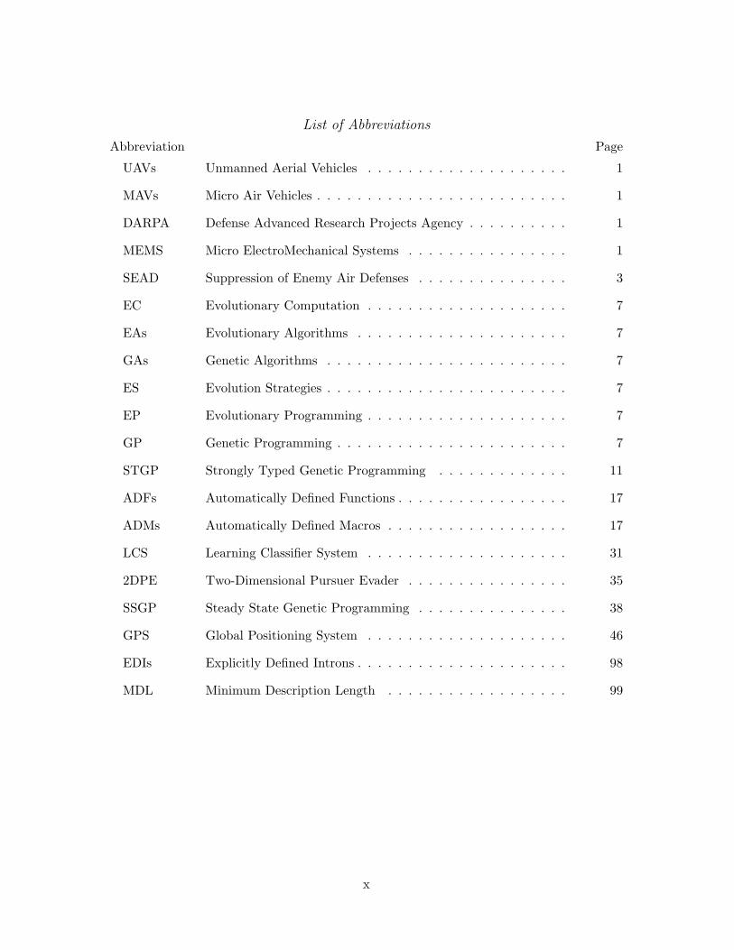
List of Abbreviations
Abbreviation Page
UAVs Unmanned Aerial Vehicles . . . . . . . . . . . . . . . . . . . . 1
MAVs Micro Air Vehicles . . . . . . . . . . . . . . . . . . . . . . . . . 1
DARPA Defense Advanced Research Projects Agency . . . . . . . . . . 1
MEMS Micro ElectroMechanical Systems . . . . . . . . . . . . . . . . 1
SEAD Suppression of Enemy Air Defenses . . . . . . . . . . . . . . . 3
EC Evolutionary Computation . . . . . . . . . . . . . . . . . . . . 7
EAs Evolutionary Algorithms . . . . . . . . . . . . . . . . . . . . . 7
GAs Genetic Algorithms . . . . . . . . . . . . . . . . . . . . . . . . 7
ES Evolution Strategies . . . . . . . . . . . . . . . . . . . . . . . . 7
EP Evolutionary Programming . . . . . . . . . . . . . . . . . . . . 7
GP Genetic Programming . . . . . . . . . . . . . . . . . . . . . . . 7
STGP Strongly Typed Genetic Programming . . . . . . . . . . . . . 11
ADFs Automatically Defined Functions . . . . . . . . . . . . . . . . . 17
ADMs Automatically Defined Macros . . . . . . . . . . . . . . . . . . 17
LCS Learning Classifier System . . . . . . . . . . . . . . . . . . . . 31
2DPE Two-Dimensional Pursuer Evader . . . . . . . . . . . . . . . . 35
SSGP Steady State Genetic Programming . . . . . . . . . . . . . . . 38
GPS Global Positioning System . . . . . . . . . . . . . . . . . . . . 46
EDIs Explicitly Defined Introns . . . . . . . . . . . . . . . . . . . . . 98
MDL Minimum Description Length . . . . . . . . . . . . . . . . . . 99
x

AFIT/GCS/ENG/04-15
Abstract
Unmanned aerial vehicles (UAVs) are rapidly becoming a critical military asset. In
the future, advances in miniaturization are going to drive the development of insect size
UAVs. New approaches to controlling these swarms are required. The goal of this research
is to develop a controller to direct a swarm of UAVs in accomplishing a given mission. While
previous efforts have largely been limited to a two-dimensional model, a three-dimensional
model has been developed for this project. Models of UAV capabilities including sensors,
actuators and communications are presented. Genetic programming uses the principles of
Darwinian evolution to generate computer programs to solve problems. A genetic program-
ming approach is used to evolve control programs for UAV swarms. Evolved controllers
are compared with a hand-crafted solution using quantitative and qualitative methods.
Visualization and statistical methods are used to analyze solutions. Results indicate that
genetic programming is capable of producing effective solutions to multi-objective control
problems.
xi

EVOLUTION OF CONTROL PROGRAMS FOR A SWARM OF
AUTONOMOUS UNMANNED AERIAL VEHICLES
1. Introduction
Unmanned aerial vehicles (UAVs), while not a new concept, have received much attention
in recent years. The very first UAVs were paper balloons used by the Austrians during
the seige of Venice in 1849. The most well known system currently in service is the RQ-
1 Predator. It has been used for operations sinced 1995 in Iraq, Bosnia, Kosovo and
Afghanistan [79]. Initially only a reconnaissance platform, the Predator was updated in
2001 to carry and launch Hellfire missiles [79]. Many other UAV platforms are being
developed to perform a variety of different missions. Currently, at least 32 nations are
developing UAV systems [79].
Micro air vehicles (MAVs) are miniature UAVs. They are generally less than 15
centimeters across with a mass of under 100 grams [37]. Advances in miniturization have
made aerial vehicles of this scale possible. In the future, UAVs the size of insects may be
feasible.
Several MAVs are currently being developed through the Defense Advanced Research
Projects Agencys (DARPA) Synthetic Multifunctional Materials program. The AeroVi-
ronment Wasp (Figure 1) has a wingspan of 13 inches and mass of 6 ounces (170 grams)
[1]. It successfully completed a 1 hour and 47 minute test flight on August 19, 2002 [1].
The Hornet (2), also from AeroVironment has a wing span of 15 inches and mass of 6
ounces (170 grams) [2]. A hydrogen fuel cell was used to power its March 21, 2003 flight.
Beyond the MAV lies the technology of micro electromechanical systems (MEMS).
This recent breakthrough in miniaturization has enabled the development of millimeter-
scale sensor nodes called “Smart Dust” (Figure 3) [48]. The target size for Smart Dust is
1 cubic millimeter [52], small and light enough to be suspended by air currents [48]. Even
beyond Smart Dust, nanotechnology may someday drive the development of still smaller
systems.
1

Figure 1 Image of AeroVironment’s Wasp MAV [1]
Figure 2 Image of AeroVironment’s Hornet MAV [2]
2

Figure 3 Image of Smart Dust “mote” [82]
1.1 Motivation
The advantages of using unmanned vehicles in the battlespace lie primarily in mission
areas commonly characterized as “the dull, the dirty, and the dangerous” [79]. A single
UAV could replace many humans assigned as sentries. This frees up scarce human resources
for other, more challenging tasks (“the dull”). In addition, UAVs can be used in areas
contaminated with nuclear, biological or chemical agents (“the dirty”). Certain high-risk
mission types, such as suppression of enemy air defenses (SEAD), can also be performed
by UAVs (“the dangerous”) [79].
As technology advances, UAVs are being assigned increasingly demanding missions.
Current UAV control systems require human operators. Such control mechanisms are not
feasible when considering hundreds or thousands of miniature UAVs, sometimes called a
swarm. This problem can be solved by adding another layer of control between the swarm
and the human operator. Instead of directing individual UAVs, the operator directs the
entire swarm. The swarm control system then determines how each individual moves based
upon the operator inputs and current state of the swarm.
3

1.2 Problem Description
The problem addressed in this research is the development of a controller for a swarm
of UAVs. Developing distributed control systems is a difficult task. Previous approaches
have used a simple series of equations to produce realistic group motion [47, 86]. Others
have used a fixed control structure and evolved values for the weight parameters [64].
This research studies the possibility of evolving the control structure itself using sensor
capabilities and movement constraints.
1.3 Goals and Objectives
The goal of this research is to develop a controller to direct a swarm of UAVs in
accomplishing user specified goals. In order to reach this goal, several objecctives must be
accomplished:
1. Develop a realistic model of UAV capabilities including sensors, communications and
movement constraints.
2. Provide a simulated environment for the development and evaluation of controllers.
3. Develop a methodology for evaluating the performance of evolved controllers.
4. Provide visualization of potential solutions.
5. Define metrics to measure performance of developed controllers.
In Chapter 3 the simulation environment is introduced along with a high level descrip-
tion of the vehicle model. This model is refined and the visualization system is discussed
in Chapter 4. The methodology and metrics used to evaluated performance are discussed
in Chapter 5.
1.4 Assumptions
There are two significant assumptions that are made in order to narrow the scope
of this research project. First, we assume that all vehicles use the same controller so
that we only deal with a homogenous swarm. In a real-world scenario, many different
complementary types of vehicles could be employed. For example, fast scout vehicles
4

could be used to locate potential targets. Then reconnissance vehicles could be used to
obtain detailed information about the targets. Finally, attack vehicles would be sent in
to destroy approved targets. The alternative is to combine many functions on a single
vehicle. It is likely that some compromise between the two extremes will prevail. One such
compromise, the Predator, is already used primarily for reconnissance but can also attack
targets of opportunity.
Secondly, an incomplete physics model is used for this research. Ignoring mass and
the effects of gravity and friction greatly simplifies the model. At the same time, it also
reduces the accuracy of the model. In many problems, there is a tradeoff between accuracy
and computational requirements that must be made. Since this research is exploratory in
nature, the reduced accuracy is acceptable.
1.5 Sponsors
The Information Directorate, Air Force Research Laboratory (AFRL/IFTA), Wright-
Patterson Air Force Base is sponsoring this research. The Information Technology Division
(IFT) conducts “broad-based R&D in information technologies to support the Informa-
tion Directorate thrusts of Global Awareness, Dynamic Planning and Execution and Global
Information Enterprise” [4]. The Embedded Information Systems Engineering Branch re-
searches and developed the technologies and processes required to engineer next-generation
weapon and information systems [3]. This research supports that mission by developing a
distributed controller for a group of autonomous vehicles. Distributed control is essential
in developing a robust system capable of dynamically adapting to changes in the mission
and/or environment.
1.6 Organization
The remainder of this thesis is organized as follows: Chapter 2 is a review of current
research in control of autonomous vehicles and genetic programming (GP). In Chapter 3,
high level models for the environment and vehicle are presented. Chapter 4 refines the high
level specification and provides details about the GP algorithm, terminal and function sets,
and system parameters. The need for a visualization environment is also discussed. The
5

design of experiments and testing proceedures used are detailed in Chapter 5. A complete
analysis of experimental results and comparison to previous efforts is also given. Chapter
6 concludes with a discussion on the impact of this research and areas where continued
study is needed.
6

2. Current Research in Control and Genetic Programming
There has been extensive research in the area of agent control. Optimization techniques
[12, 13, 46], neural networks [38], rule based systems [17, 18, 29, 105], swarm systems
[20, 31], emergent behavior approaches [28, 36, 47, 64, 86] and genetic programming [5, 6,
69, 74, 97] are some of the methods which have been applied. This chapter begins with
a brief overview of genetic programming. Then contemporary research on agent control
systems is reviewed.
2.1 Discussion of Genetic Programming
This section provides a brief discussion of the origins of evolutionary computation.
The early development of genetic programming is presented, followed by a description
of the GP algorithm. Different genetic operators and individual representations are also
surveyed.
2.1.1 Evolutionary Computation. The notion of evolutionary computation (EC)
as a unified field of study appeared for the first time 1991 as a way to unite researchers
interested in simulating evolution [9]. Common among all approaches within EC are the
principles of Darwinian evolution: reproduction, random variation, competition and selec-
tion. Evolutionary computation includes the study of evolutionary algorithms (EAs) such
as: genetic algorithms (GAs), evolution strategies (ES), evolutionary programming (EP)
and genetic programming (GP).
Genetic programming is the process of evolving computer programs (trees) to solve
problems. The automatic generation of computer programs has long been a goal in Com-
puter Science. Arthur Samuel in his pioneering 1959 work on machine learning [90] states
that it “is necessary to specify methods of problem solution in minute and exact detail, a
time-consuming and costly procedure. Programming computers to learn from experience
should eventually eliminate the need for much of this detailed programming effort” [53].
Even before that though, Alan Turing considered the idea that computers might use
a biological approach [54]. In his 1948 essay “Intelligent Machines”, Turing stated that
“Further research into intelligence of machines will probably be very greatly concerned
7

with ’searches’ ” [54]. He went on to describe three general types of search. The first
type is essentially a search through all possible Turing Machines. The second approach is
the “cultural search” that uses information gained through prior experience to guide the
search. The final approach is the “genetical or evolutionary search.” Turing said [53],
There is the genetical or evolutionary search by which a combination ofgenes is looked for, the criterion being the survival value. The remarkablesuccess of this search confirms to some extent the idea that intellectual activityconsists of various kinds of search.
Though Turing did not define how the evolutionary search would work, some clarification
is found in his 1950 paper “Computing Machinery and Intelligence” [54].
We cannot expect to find a good child-machine at the first attempt. Onemust experiment with teaching one such machine and see how well it learns.One can then try another and see if it is better or worse. There is an obviousconnection between this process and evolution, by the identifications
Structure of the child machine = Hereditary material
Changes of the child machine = Mutations
Natural selection = Judgment of the experimenter
It is unclear wether Turing’s work served as inspiration for the development of EA as
we know them today. Other attempts at evolving computer programs include Friedberg’s
efforts using a hypothetical language [53]. Friedberg used random initialization and mu-
tation to create and evolve his test programs. The programs were executed and evaluated
based on their performance, all-or-nothing in this case. While Friedberg’s work exhib-
ited some aspects of GP, it lacked the concepts of reproduction, population, generations,
memory of genetic information and crossover [53].
Another attempt to apply evolution to the task of developing artificial intelligence
came from L. J. Fogel in the 1960s [8, 9, 53]. In one example, Fogel, Owens and Walsh [32]
evolved finite-state machines (FSM) as predictors for primality [9]. An initial population
of FSMs was randomly generated. Each individual FSM in the population was tested on
the inputs and given a score based on performance. Offspring were generated via mutation
on aspects of the FSM. The offspring were evaluated like the parents. Individuals with the
highest fitness were selected for the next generation. This technique is called evolutionary
8

programming. It is quite similar to GP, except for the lack of a crossover operation and
the difference in genotype representation.
Despite striking similarities which exist between GA, ES and EP, they were all de-
veloped independently [8]. The ES and EP communities developed in Europe, while the
GA community started in the United States. Genetic programming grew out of work on
GAs [9, 60, 53]. The seminal work in GAs is the 1975 book Adaptation in Natural and
Artificial Systems by John H. Holland [41].
In a GA system, individuals, or chromosomes, are represented as an array of bits.
The genotype is given by the value of the bit strings. The genotype is interpreted to pro-
duce an individual’s phenotype, or behavior. The fitness of an individual in a particular
environment is based on its behavior. After all individuals in a population (µ) have been
evaluated, a fitness-based selection method is used to choose parents for the next genera-
tion. Genetic operators, crossover and mutation for standard GAs, are then applied to the
parent chromosomes to create the children (λ). Crossover is heavily favored for GA, with
mutation used mainly as a way to maintain some genetic diversity in the population. The
situation is reversed for ES, where mutation is the primary genetic operator and crossover
is seldom used.
Members of the next generation are chosen, based on fitness, from the current gener-
ation and the children; (µ + λ) → µ. An alternative approach is to only select members of
the next generation from the set of offspring; (µ, λ) → µ. The selection process continues
until the population has converged on a solution, or a predetermined number of generations
has been evolved [8, 9, 41]. Increasing the mutation rate, reinitializing the population, us-
ing different genetic operators or different system parameters are all approaches used to
cope with premature convergence [9].
2.1.2 Early Genetic Programming. Genetic Algorithms have been modified and
expanded in various ways over the years [9, 53]. Different types of mutation and crossover
operators, and entirely new operators have been developed and tested. Significant for GP
is the study of alternative representations as well as variable length chromosomes. Strings
of 1s and 0s can be used to encode integers, real numbers, permutations or even computer
9

instructions [27, 9]. Nichael L. Cramer in his 1985 paper A Representation for the Adaptive
Generation of Simple Sequential Programs [27] described the first GP approach. Cramer’s
goal was to use a simple programming language “suitable for manipulation by GAs” [27]
to evolve useful functions from low-level primitives.
Two important characteristics of such a system were identified [27]. First, it must
work with the standard genetic operators of GAs. A method of encoding the computer
language instructions as binary strings had to be devised. The second requirement was
that all resulting individuals must be syntactically correct programs. This means that
there must be some way to decode the binary strings generated by the GA as a valid
program in the chosen language.
Cramer’s first attempts used a language called JB, based on the algorithmic language
PL. The standard GA genetic operators did not work effectively with the linear integer
representation used by JB. In an attempt to remedy the problems, Cramer devised the TB
language. This language used the tree-like representation which is familiar in GP today.
Modifications were also made to the standard genetic operators in order to allow them to
work with the new representation.
Initial tests using this new tree-based GA approach were encouraging. Cramer used
his system to evolve the multiplication function. His system succeeded 72% more often
than random program generation. Cramer’s work highlighted the need to evolve programs
using a higher level representation than binary strings. He also illustrated the convenience
of the tree or nested list representation.
In 1986, Hicklin applied Cramer’s work to LISP programs [53]. He implemented an
evolutionary system with mutation and reproduction. Also in 1986 Fujiki, and later in
1987, Fujiki and Dickenson extended Hicklin’s efforts by adding crossover and inversion to
the set of genetic operators [53].
John R. Koza is generally acknowledged to be the father of genetic programming.
The GP system he described is considered to be the standard, much as Holland’s GA is
considered standard. In his 1992 book Genetic Programming: On the Programming of
Computers by Means of Natural Selection [53], Koza explained GP and made the first
10

comprehensive attempt to explain why it works [60]. Acknowledging the close relationship
to GAs, Koza extended the Schema Theorem to GP. The Schema Theorem provides a
method to calculate the expected number of building blocks, or good combinations of
alleles, for each generation in a genetic algorithm.
2.1.3 Detailed Description of Genetic Programming. The goal of genetic pro-
gramming is for computers to automatically produce program solutions. Human beings
are still needed to provide expertise to the system in order to achieve reasonable results.
Inputs to a GP system include: set of functions, set of terminals, fitness evaluation, sys-
tem parameters and success or stopping criteria [53]. The values chosen for these inputs
ultimately determine the success or failure of the search. Exact values for these inputs are
highly problem domain dependent and are discussed in detail in Chapters 3 and 4.
Genetic programming uses evolutionary forces to guide the search for good solutions.
Solutions in GP are computer programs. The programs that can be generated by a given
GP depend on the set of functions (F) and terminal symbols (T ) that are made available.
Decisions regarding specific terminals and functions are problem dependent and considered
further in Chapter 4.
Good function and terminal sets must satisfy two important properties: closure and
sufficiency [53]. The closure property dictates that every function in F must accept as
input the return value from any functions or terminals. This property is easily satisfied for
simple problems, such as those involving only boolean functions and the terminals “true”
and “false”. When numbers are involved, ensuring the closure property holds is slightly
more tricky. For instance if division is included in F , a special measures must be taken to
handle division by zero [53]. In Koza’s original work [53] only one data type was allowed
for a program. Subsequent research by Montana on strongly typed genetic programming
(STGP) [73] shifted the burden of closure away from the user onto the GP system.
The second important property of the function and terminal sets is sufficiency [53].
Sufficiency means that the functions and terminal symbols used are able to represent the
specified goal. To illustrate this concept, suppose we have F = +, * and T = x, y
11

(x, y ∈ R). The goal function is subtraction (x - y). There is no way subtraction could be
evolved in this case without the negation operator.
After defining the function and terminal sets, the initial population can be created.
Two common methods for generating a new random program tree are the “full” method
and the “grow” method [53]. The full method creates trees such that all paths from leaf
nodes to the root are the same length. This is done by restricting the choice of values for
nodes less than the maximum depth to F . Node values at the maximum depth are chosen
from T .
The grow method creates trees such that paths from leaf nodes to the root vary in
length. Like the full method, a maximum depth is selected. Values for nodes with depth
less than the maximum depth are selected from F∪T . Node values at the maximum depth
are chosen from T [53].
Often, the grow and full methods are combined into the “ ’ramped half-and-half’
generative method” [53]. A minimum and maximum depth parameter are used in order
to create trees of different depths. A depth value is randomly chosen over the interval:
[minimum depth, maximum depth]. The decision of which initialization method to use
is also made randomly. Suppose the minimum depth value is 5 and the maximum depth
value is 8. The expected distribution of tree sizes would be: 25% each of depths 5 - 8.
Approximately half of the trees of each depth would be created using the full method and
the other half using the grow method. Alternatively, fixed values may be used to guarantee
these expected distributions.
In order to better illustrate how individuals are evaluated in GP, it is helpful to use
a couple of example problems. Figures 4 and 5 show two program trees for the symbolic
regression problem and artificial ant problem respectively. The symbolic regression problem
is essentially a curve matching problem [53]. Given a set of values for x and y, what is the
function f() where f(x) = y? In Figure 4, f(x) = 5 + ((8− x) ∗ x).
The artificial ant problem is also well known. An ant is placed on a discrete, torroidal
map. Food is placed in the squares to form a non-contiguous trail. The goal is for the ant
to gather all of the food in the shortest amount of time. A typical instantiation of this
12

Figure 4 Sample symbolic regression program tree [53]
Figure 5 Sample artificial ant program tree [53]
problem is the “Santa Fe Trail” which uses 89 pieces of food [53]. The ant has the ability
to see what is in front of it, to turn left or right and to move straight ahead.
These are good example problems, but they are not the only classes of problems used
in GP. One can also interpret the evolved programs as assembly instructions. Koza uses
this technique in evolving electronic circuits [54].
After initialization, each individual (program) in the population is evaluated. In
GP, this is done by executing the program tree. Each internal node, which is always a
function, evaluates its subtrees and after performing any required calculations, returns
a value. Leaf nodes, which are always terminals, are evaluated directly. In the case of
symbolic regression, the leaves represent real numbers and the internal nodes represent
13
IF-FOOD-AHEAD
MOVE TURN RIGHT

arithmetic functions such as addition, multiplication and sine. The value of each node
depends on the value of its subtrees.
Evaluation of the artificial ant problem is slightly more complex. The ant must move
around on a simulated map looking for food. Each action the ant takes, such as turning to
the right, left or moving forward counts as a move. While evaluating the tree, the ant is
directed around the map. After the tree has been evaluated, the ant has completed some
number of moves, mi. However, mi is typically much less than the total number of moves
allowed mT . To resolve this, the program is executed repeatedly until either the maximum
number of moves has been made or all the food has been gathered.
After the stopping criteria have been met, the performance of the program is mea-
sured. For the symbolic regression problem, performance might be measured by the error
between the program’s return value and the true function value. Performance for the
artificial ant problem is typically measured as the amount of food gathered.
All individuals in the population are similarly evaluated. Assuming that no programs
have solved the problem, the next generation is created. To create the new population,
first a genetic operator is chosen based on assigned probabilities. Figures 6 through 8
illustrate the crossover and mutation operations. The reproduction operator simply copies
the selected individual.
The appropriate number of individuals for the chosen operator are selected from
the current population. Next, the genetic operator is applied and then the individuals
are placed in the new population. After the new population has been generated, the
fitness evaluation is repeated. This process continues until either a solution is reached or
a maximum number of generations has been evolved. The symbolic representation of the
genetic programming algorithm using Back’s notation is given in Appendix B.
2.1.4 Genetic Operators. The genetic operators reproduction and recombination
are viewed as the primary operators in GP [9, 53]. Like GAs, a low rate of mutation is
typically desired [41, 53]. In fact, mutation is deemed a “secondary operator” by Koza,
and often not used at all [53, 69, 87]. Koza advocates fitness-proportional selection in [53],
but other methods such as tournament selection [9, 69, 70] have also been applied.
14

Figure 6 Two program trees before crossover. Highlighted nodes are the chosen crossoverpoints. [53]
Figure 7 Two program trees after crossover [53]
15
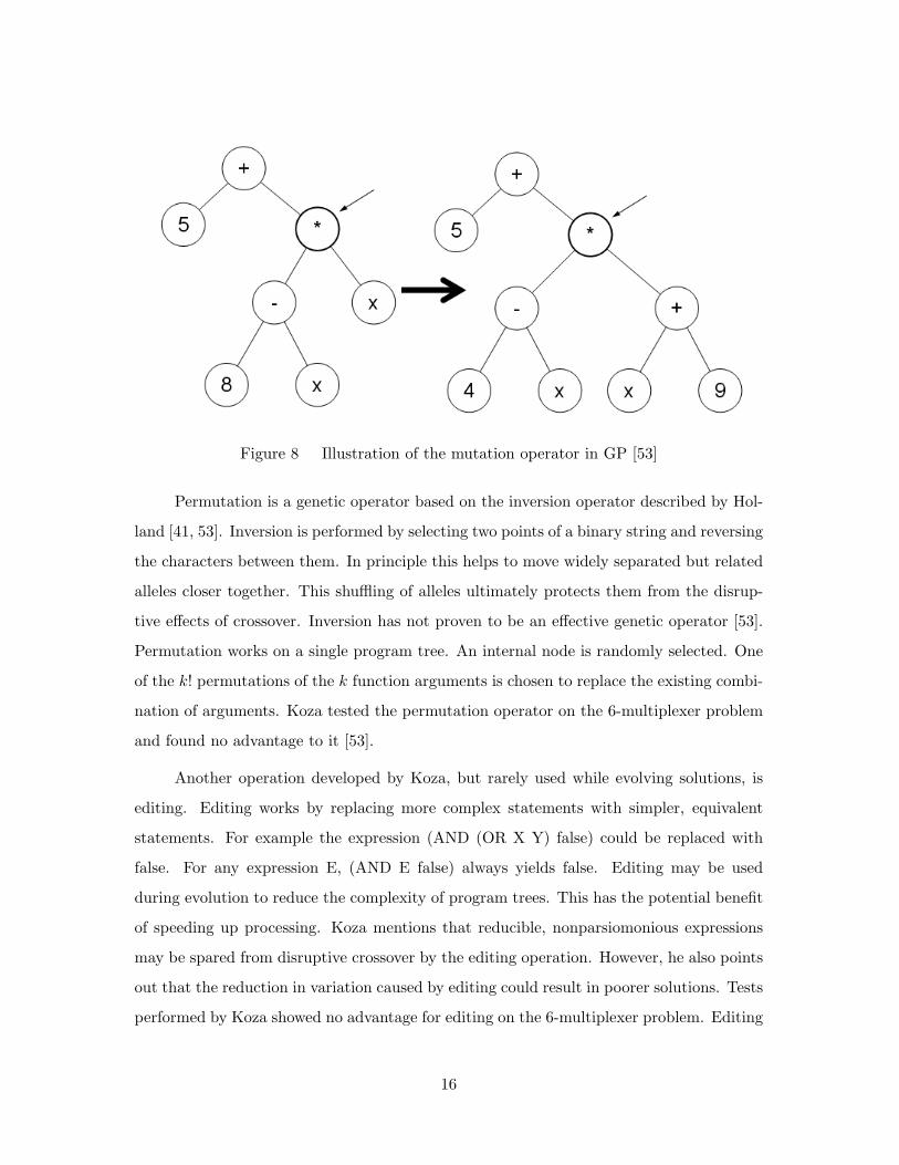
Figure 8 Illustration of the mutation operator in GP [53]
Permutation is a genetic operator based on the inversion operator described by Hol-
land [41, 53]. Inversion is performed by selecting two points of a binary string and reversing
the characters between them. In principle this helps to move widely separated but related
alleles closer together. This shuffling of alleles ultimately protects them from the disrup-
tive effects of crossover. Inversion has not proven to be an effective genetic operator [53].
Permutation works on a single program tree. An internal node is randomly selected. One
of the k! permutations of the k function arguments is chosen to replace the existing combi-
nation of arguments. Koza tested the permutation operator on the 6-multiplexer problem
and found no advantage to it [53].
Another operation developed by Koza, but rarely used while evolving solutions, is
editing. Editing works by replacing more complex statements with simpler, equivalent
statements. For example the expression (AND (OR X Y) false) could be replaced with
false. For any expression E, (AND E false) always yields false. Editing may be used
during evolution to reduce the complexity of program trees. This has the potential benefit
of speeding up processing. Koza mentions that reducible, nonparsiomonious expressions
may be spared from disruptive crossover by the editing operation. However, he also points
out that the reduction in variation caused by editing could result in poorer solutions. Tests
performed by Koza showed no advantage for editing on the 6-multiplexer problem. Editing
16

is often performed at the end of GP runs, resulting in a more efficient and easier to read
solutions [53].
The encapsulation operation is used to allow entire subtrees to be reused. First an
internal node is randomly selected in the tree. The subtree rooted at that node is removed.
A new identifier is created which references the removed subtree. This identifier is inserted
into the tree at the previously selected node. The identifier is added to the set of terminal
symbols and can be used in future mutation operations. Encapsulation provides a method
of evolving reusable functions. No significant difference is noted the performance of the
6-multiplexer problem by adding encapsulation [53].
The assembly of complex systems using simpler components can be found almost
everywhere. A stereo for instance uses an amplifier. The amplifier is in turn made up of
simpler electronic components. Complex organisms like mammals are made up of billions
of cells, which are in-turn composed of smaller elements like DNA or mitochondria. The
idea of identifying and reusing useful building blocks exemplified by the encapsulation op-
eration is expanded upon with the addition of automatically defined functions (ADFs) and
automatically defined macros (ADMs). Other techniques, including Module Acquisition,
have been proposed [96].
The distinction between encapsulation and ADFs is that ADFs are parameterized
functions, while encapsulation accepts no arguments [53]. Automatically defined functions
and macros allow increased generalization. Encapsulation may allow the calculation of
the square of a specific variable, x : (∗xx). Using ADFs, this function can be applied to
any variable, X: (* X X). If the square function is needed for multiple variables, the more
general ADF form would be preferred. This saves the effort required to evolve specialized
functions for specific variables. Tests performed by Koza showed that ADFs can enhance
the performance of GP on even parity problems [53].
Automatically defined macros are very similar to ADFs. Both are used to exploit reg-
ularities in problem domains by increasing the modularity of solutions[96]. One advantage
of using macros instead of subroutines is that macros can create new control structures.
Arguments to ADMs are not evaluated before being passed into the procedure. Consider
17

the function “do-twice”, which takes a single argument and evaluates it two times. If the
argument were an expression, such as (add X 5), the ADM has the effect of adding 10 to
X. The ADF is given the argument 15 (when X = 10) because arguments are evaluated
before being passed to the function [96]. Tests comparing ADFs and ADMs showed that
ADMs may have slight advantages in certain problem domains [96].
2.1.5 Alternative Representations. Individuals in GP are computer programs.
They are typically represented as trees, but other representations have been used [60, 53].
Langdon and Poli provide a brief description of alternative representations in their book
Foundations of Genetic Programming [60]. The most common representation other than
trees is as a linear chromosome. This is very similar to the standard GA representation.
In fact, this is the approach Cramer used in his work [27]. Instead of a fixed length
chromosome of conventional GAs, the length is variable. Langdon and Poli divide the
linear approaches into three broad categories: stack based, register based and machine
code.
Stack-based GP, as the name implies, uses a stack to perform calculations and store
results [81]. The original stack-based GP by Perkis used a variable length, linear sequence
of functions and terminal symbols. Terminals, which were all variables, were pushed on the
stack. Functions would pop values from the stack and push results back on. If there were
not enough values on the stack, the function was simply ignored. Programs were evolved
using the standard genetic operators from GA. Perkis acknowledged that an obvious limi-
tation of this initial system was the lack of branching constructs [81].
The Push programming language was developed by Lee Spector specifically for use
in evolutionary computation systems [98]. The Push language is loosely based on LISP.
It supports use of multiple data types, modularity, control structures like branching and
recursion and autoconstructive evolution [98, 97]. Spector defines an autoconstructive
evolutionary system as “any evolutionary computation system that adaptively constructs
its own mechanisms of reproduction and diversification as it runs” [98].
The PushGP system is used to evolve Push programs [96]. Unlike Perkis’ system, it
uses multiple stacks, one for each data type. Looping and recursion are enabled through
18
the addition of a special “CODE” stack. Push programs are hierarchical, using parentheses
to group statements. This hierarchical nature allows Push programs to be viewed as trees.
The genetic operators are analogous to those of standard GP. A performance comparison
between PushGP and Koza’s conventional GP was made using N-even-parity problems
[98]. Results showed that the PushGP system scaled better as the number of inputs (N)
increased.
Register-based and machine-code GP are very similar [60]. Both methods use reg-
isters to store and retrieve data. Inputs to the program are stored before the program is
executed and the results are stored in registers upon completion. The distinction between
the two is that machine-code GP uses actual machine specific hardware instructions. In-
structions in register-based GP (and all other GP) are either compiled or interpreted, not
directly executed. Due to the direct implementation, machine-code GP typically executes
ten to twenty times faster than other methods [60].
In addition to linear and tree-like representations, GP systems have also been de-
veloped using graph-based representations [60, 83, 100]. The PDGP (Parallel Distributed
Genetic Programming) system was presented by Poli in 1997 [83]. Nodes in the evolved
graph represent the functions and terminals. The directed edges between nodes indicate
the flow of arguments and results. A “grid” is used to arrange the nodes. Nodes in the
graph connected to the output node are considered active. The other nodes in the graph
serve as introns. Crossover operates by inserting a randomly selected subgraph of one par-
ent into a random point in the other parent. Mutation is performed by either modifying
an edge in the graph or inserting a randomly generated subtree [83].
Tests performed using Koza’s lawnmower problem showed that PDGP was more
effective at finding solutions [83]. Furthermore, PDGP produces results that can easily
be transferred to parallel computing platforms [83]. The PDGP system is not limited to
evolving program graphs. Graphs interpreted as neural nets, semantic nets or finite state
automata are also feasible [83].
Teller’s PADO (Parallel Architecture Discovery and Orchestration) system has pri-
marily been used in image and signal recognition tasks [60, 100]. Unlike PDGP, nodes in
19

PADO are not restricted to a grid. In addition to the type and connections between nodes,
the number and and locations are also evolved. A final difference is that while edges in
PDGP represent data paths, edges in PADO represent control paths [83]. A decision is
made at each node that determines the edges that are followed during execution of the
program [100].
Strongly typed genetic programming is an extension to standard GP based on Koza’s
“constrained syntactic structures” [53, 73]. Constrained syntactic structures are based on
the idea that certain problems either require or benefit from the use of a certain tree
structure. The problems used by Koza to illustrate this concept focused on programs that
returned multiple values. The root node was constrained to ensure the appropriate number
of values were generated [53].
With STGP, each terminal, function argument and function return value has an
assigned type [73]. The genetic operators are modified to ensure that consistency is main-
tained. This means, for instance, that a subtree which returns an integer value could not
be swapped into a position expecting a real valued argument. Strongly typed GP is a
useful approach for handling problems that use multiple data types.
One of the major concerns in Genetic Programming is the size of evolved solutions.
As an evolutionary trial progresses, the size of program trees grows larger without a corre-
sponding increase in fitness [58]. Large programs take longer to evaluate resulting in poor
scalability. They also tend to have a large number of unused instructions, referred to as
introns [78, 95]. A significant amount of research has been performed with respect to this
difficult problem [14, 93, 58, 59, 67, 78, 95]. Additional discussion of this topic can be
found in Appendix C.
2.2 Symbolic Description of Problem Domain
The goal of this research is to develop a controller for an autonomous air vehicle.
A swarm of UAVs each using the developed controller is instantiated in a simulated envi-
ronment. The environment is a three-dimensional space containing one or more goals (or
targets), threats and waypoints. A set of capabilities and constraints is associated with
20

each vehicle type. In addition to the individual behavior of each vehicle, we are interested
in the overall behavior of the swarm.
The problem domain can be symbolically described by the tuple (V, C, G, W, T, O,
S, R) [64], where:
V is the set of all vehicles:
Vx is the set of all vehicles of type x;∀x, y Vx⋂
Vy = ∅ where 0 ≤ x 6= y ≤ n,⋃ni=0 Vi = V and
⋃mj=0 vxj = Vx where n is the number of distinct vehicle types
and m is the number of vehicles of type x;
G is the set of goals;
W is the set of waypoints w ∈ W |the set of all waypoints;
T is the set of threats t ∈ T |the set of all threats;
O is the set of obstacles o ∈ O|the set of all obstacles;
Sx is the set of capabilities possessed by vehicles of type x;
Rx is the set of constraints imposed on vehicles of type x;
Cx is the controller for vehicles of type x.
The controller Cx generates an output signal using sensor inputs (Sx) and information
about the goals (G), waypoints (W), obstacles (O) and threats (T). The control signal
is used to alter the behavior of vehicle i of type x (vxi), according to the movement
constraints , vehicular constraints (Rx). In addition to objective measurements of controller
performance, subjective qualities are examined. Emergent swarm behavior is analyzed
visually and compared with natural and artificial systems.
2.3 Contemporary Research on Autonomous Agent Control
Autonomous agent control has been extensively studied by many researchers. Several
different approaches have been used to successfully control autonomous agents. The review
of these techniques is arranged according to the algorithms used for agent control and the
methods used for generating the controller.
21

Dudek, et al have proposed a taxonomy for multirobot systems [30]. They use the
following attributes for system classification: size, communications range, communications
topology, communication bandwidth, collective reconfigurability, processing ability and
collective composition [30]. These and other aspects of the reviewed systems are discussed.
A summary is provided in table X.
2.3.1 Swarm Systems. Swarm intelligence is an approach to problem solving
modeled inspired by the behavior of natural systems like ant colonies [102]. These systems
exhibit the “phenomenon of self-organization” [102]. This enables individuals to produce
complex group behavior without using a centralized control mechanism. Decentralized
architectures are fault tolerant, reliable, scalable and are able to exploit the inherent par-
allelism of the swarm [20].
Cao et al., reviewed the field of cooperative mobile robotics, giving examples of
several projects [20]. One project mentioned was a behavior-based approach by Parker.
The ALLIANCE architecture was developed in which robots used sensors and broadcast
communications to determine a set of behaviors to apply. Reinforcement learning was
added (L-ALLIANCE) to allow modification of the rule set activation parameters [20].
Another behavior-based approach proposed by Mataric was also cited by Cao et al.,
[20]. Collective behaviors were generated by combining simpler, more basic behaviors. An
automated procedure to develop these behavior combinations using reinforcement learning
was also presented [20]. Both simulated and physical implementations have been per-
formed.
The organization of individuals in the swarm is another aspect which has received
attention [20]. The formation and marching problems are concerned with organizing mem-
bers into specific configurations and then moving as a single unit while maintaining the
prescribed patterns [20]. Trianni et al., studied the aggregation behavior of a swarm of
s-bots, “mobile robots with the ability to connect to / disconnect from each other” [102].
Using an evolutionary approach, they found two distinct types of behavior: static and
dynamic clustering. The static clusters were very compact, having little space between the
22

vehicles. Vehicles were spaced further apart in the observed dynamic clustering behavior.
Dynamic clustering was shown to allow more scalability [102].
Movement in formation was explored by Baldassarre et al., [11]. Four Khepera robots
with homogenous controllers were used in the experiments. The controller was evolved
using neural networks [11]. Three distinct, successful formation behaviors were evolved
which showed that, contrary to previous claims by Zaera et al., “artificial evolution is
an effective method for automating the design process of robots able to exhibit collective
behaviours” [11].
In their introduction, Feddema et al., state that increasing attention is being given
to analysis of the stability of multi-vehicle formations [31]. Centralized and decentralized
control laws have been used to drive vehicles into circular formations and away from
obstacles [31]. Feddema et al., also cite the combination of graph theory and decentralized
control as a recent area of research.
2.3.2 Mathematical Optimization. Mathematical optimization techniques at-
tempt to find optimal, or near optimal, solutions to the agent control problem. This is
achieved by solving, or approximating, some cost minimization function. One disadvantage
of this approach is that it is computationally demanding [12]. The amount of computation
required often grows exponentially with respect to the number of inputs, quickly becoming
intractable. Fortunately, approximation techniques can provide acceptable solutions in a
reasonable amount of time [13].
Another common aspect of the optimization projects reviewed is centralized compu-
tation. A central controller is responsible for performing calculations and distributing a
solution to individuals in the system [12, 13, 46]. This centralized approach is vulnerable to
failure of the central controller or communications system. Thus, while the entire system
can operate autonomously, the individual vehicles are not fully autonomous.
In [12], Bellingham et al., present a solution to the multiple task allocation and path
planning problem. The path planning subproblem is described by the following equations:
t = maxp
tp (1)
23
J1(t, t) = t +α
NV
NV∑p=1
tp (2)
where α 1 is the weight given to the average completion time, tp is the time vehicle p
completes its mission, NV is the number of vehicles and t is a vector of the finishing times
for each vehicle [12]. The parameter α must be determined experimentally and is likely
problem dependent.
Detailed trajectories determine depend upon the ordering of tasks or mission ob-
jectives. The task allocation process is formulated as a multi-dimensional multiple-choice
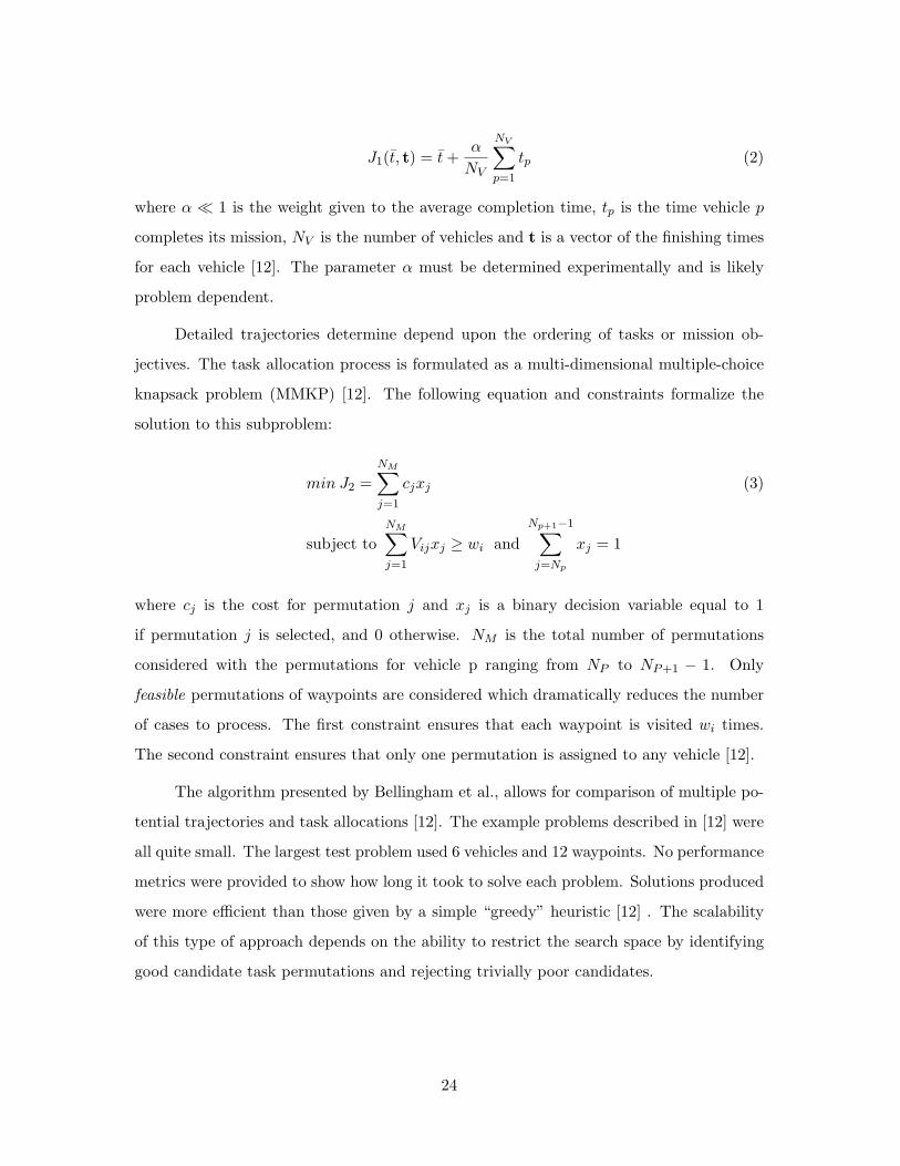
knapsack problem (MMKP) [12]. The following equation and constraints formalize the
solution to this subproblem:
min J2 =NM∑j=1
cjxj (3)
subject toNM∑j=1
Vijxj ≥ wi andNp+1−1∑j=Np
xj = 1
where cj is the cost for permutation j and xj is a binary decision variable equal to 1
if permutation j is selected, and 0 otherwise. NM is the total number of permutations
considered with the permutations for vehicle p ranging from NP to NP+1 − 1. Only
feasible permutations of waypoints are considered which dramatically reduces the number
of cases to process. The first constraint ensures that each waypoint is visited wi times.
The second constraint ensures that only one permutation is assigned to any vehicle [12].
The algorithm presented by Bellingham et al., allows for comparison of multiple po-
tential trajectories and task allocations [12]. The example problems described in [12] were
all quite small. The largest test problem used 6 vehicles and 12 waypoints. No performance
metrics were provided to show how long it took to solve each problem. Solutions produced
were more efficient than those given by a simple “greedy” heuristic [12] . The scalability
of this type of approach depends on the ability to restrict the search space by identifying
good candidate task permutations and rejecting trivially poor candidates.
24

The application of probabilities to the path planning problem is a natural extension.
The real world is an uncertain place. Bombs don’t always destroy their target. Probabilities
allow the representation of uncertainty. This is especially important when considering the
likelihood of mission success. Missions with a low chance of success may be modified with
additional vehicles or fewer targets.
Jun and D’Andrea developed a system using a probability map [46]. The environ-
ment under consideration is split into regions or cells of equal size. Each cell has a three
associated probabilities: a vehicle is detected while in the cell, the cell is occupied by an
enemy and the vehicle is destroyed by the enemy [46]. It is assumed that some mechanism,
such as intelligence gathering or surveillance, exists for determining the probabilities of
these events. The probability map is converted to a digraph. The edge weights are derived
from the above probabilities. This transforms the problem into that of finding the short-
est path between two nodes [46]. The shortest path problem can be easily solved using
Djikstra’s algorithm or the Bellman-Ford algorithm.
One limitation of this work is that only a discrete, two-dimensional map was con-
sidered. In addition, only scenarios with a single target were discussed. Multiple vehicles
were considered, but still relied on a centralized control system. Despite these concerns, the
research illustrates that probabilities can be effective in solving path planning problems.
Bellingham also extended his original path planning algorithm [12] to include uncer-
tainty [13]. A “stochastic optimization formulation” is presented that takes into account
changes in probabilities as the environment is modified. An example of this is the destruc-
tion of an anti-aircraft site. Vehicles moving through a defended region will have different
survival probabilities than vehicles moving through after the anti-aircraft systems have
been destroyed [13].
Previous work used a simpler model which did not take such changes into account
[13]. The new stochastic approach produced significantly better plans, but also required
approximately 4 times the computational effort. This work uses a continuous space instead
of a discrete grid. It also uses a rich, dynamic simulation environment with different types
of vehicles and objectives [13].
25
2.3.3 Subsumption Architecture. A unique approach to robot control was dis-
cussed by Brooks [16]. The traditional approach was to decompose behavior into functional
units. Separate modules were used for perception, modeling, planning, task execution and
motor control [16]. These modules were connected serially. For example, the modeling
subsystem would create a model of the current situation. The model would then be passed
to the planning module, which would generate an appropriate plan.
In contrast, Brooks proposed decomposing problems based on task achieving behav-
iors [16]. Different modules included: avoid objects, wander, explore, build maps, monitor
changes, identify objects, plan changes to world and reason about behavior of objects [16].
These modules are arranged in parallel and can work simultaneously to solve problems.
This is called the subsumption architecture.
One advantage of the subsumption architecture is that more complex behaviors are
developed in a bottom-up approach. Basic behaviors such as obstacle avoidance can be
developed and tested without implementing higher level behaviors [16]. This technique
allows a form of distributed control where the results of various subsystems are combined
to determine the action of the system. The idea of complex behavior resulting from the
interplay of simple actions is common in swarm research [20, 86, 102].
The subsumption approach was used by Lua et al., to control UAVs [65]. Their
objective was to develop a control mechanism to perform a synchronized, multi-point
attack using only local communication. The behaviors of: avoid, attack, orbit station,
orbit target and search were defined and implemented [65]. Appropriate behaviors are
selected using the sensor inputs and current state of a vehicle. For example, if two vehicles
move too close to one another, their avoid behavior is activated until the problem has been
remedied.
The approach used by Lua et al., was effective at coordinating a near simultaneous
attack of multiple UAVs using local communications without a centralized control mecha-
nism [65]. Simulations using 5 and 18 UAVs to attack a single, stationary target showed
that this approach is effective and scalable [65]. Human operators must still design the
behaviors and how they influence and subsume one another. Depending on the mission
26

and environment, it may not always be easy, or possible to produce the behaviors and
relationships. One way around this problem is to use the computer to produce a solution.
2.3.4 Neural Networks. Research by Harvey et al., discusses why producing
control systems is difficult and reviews possible solutions [38]. It is difficult to foresee all
possible ways an agent might interact with an environment. The complexity involved in de-
signing cognitive architectures can “scale with the number of possible interactions between
modules” [38]. Solutions to such a problem require either an intractable computational
effort or a non-generalizable, “creative act” [38].
The process of evolution is suggested as an alternative to both functional and sub-
sumption approaches. One can use evolutionary forces to guide the search for a solution.
Simulation is recommended as the best means of evolving control systems due to time
and resource constraints required for real world evaluations. As much realism as possible
should be maintained in the simulation to facilitate the transfer of results into the real
world [38].
The genetic programming approach is rejected for several reasons. First, programs
which support looping constructs fall victim to the halting problem. This has been reme-
died by simply not allowing looping or interrupting programs after a certain time limit.
The authors also object to treating the brain as a computational system. They believe
it should be treated as a dynamical system instead [38]. Whether or not this is the case,
GP has produced patentable, human competitive results [54]. The final objection is about
the language under consideration. The languages BL and GEN are discounted as being
too high level to effectively evolve solutions. There is no reason that alternative language
constructs cannot be used instead of those proposed by Brooks [38].
The chosen solution structure was a neural network. The number and type of internal
nodes was evolved as well as the number and weights of links between the nodes. Neural
networks evolved the ability to avoid obstacles, maximize distance from the starting point
and maximize the area circumscribed by the robot’s path [38]. One difficulty with neural
networks is analyzing them to determine how they function. This is possible with small
27

networks, but difficult at best for those of moderate size. The authors conclude, “Artificial
evolution seems a good way forward” [38].
2.3.5 Artificial Immune Systems. Natural immune systems are the inspiration
for another evolutionary approach to robot navigation. In immune systems, antibodies
are detectors for antigens. Once an antibody detects an antigen, an immune response is
activated. This process can be used in robot navigation as well. Robot sensor information
corresponds to antigens. Antibodies are represented as patterns which match potential
sensor inputs and have specific actions associated with them [104]. Antibodies may also
stimulate or suppress other antibodies. This forms a complex network which enables the
emergence of highly complex behavior [104].
When an antigen is detected, the strength or concentration of all antibodies is calcu-
lated. The result depends heavily on the network of connections between antibodies. The
following equations are used [104]:
dai(t)dt
=
N∑j=1
mjiaj(t)−N∑
k=1
mikak(t) + mi − ki
ai(t) (4)
ai(t) =1
1 + exp(0.5− ai(t))(5)
where:
N, number of antibodies in the network;
mi, affinity between antibody i and the given antigen;
mji, affinity between antibodies j and i, the degree of stimulation;
mik, affinity between antibodies k and i, the degree of suppression;
ki, natural death coefficient of antibody i.
Roulette-wheel selection is then performed to select the antibody that will be activated.
Once an antibody is selected, its associated action is performed by the robot.
The network of connections between antibodies is modified using a genetic algorithm
[104]. Individuals are composed of a group of antibodies. Crossover exchanges a randomly
28

determined number of antibodies between two selected groups. Mutation can operate in
two ways. First, a single network connection in an antibody can be modified. Second, any
number of network connections in an antibody can be deleted.
Experiments were performed using the garbage collection problem [104]. The robot
must move through a simulated environment, collect garbage and return it to the base.
Performance of the evolved immune network was compared to that of an immune network
designed with expert information [104]. The evolved network was able to perform the same
task at or above the level of the hand coded system. Another experiment showed that an
immune network enabling a robot to follow a moving object could be evolved using only
mutation [104]. Tests using a Khepera II robot were performed to show that an evolved
network can be used to control a real robot.
One of the limitations of the approach described is that neither the sensor/action
pairs nor the antibodies were evolved [104]. In order to completely search the space,
all possible sensor/actions pairs and antibody patterns must be included. Alternatively,
expert knowledge could be used to select the patterns to include. It is also difficult to see
how even simple immune networks determine which actions to take. The decision process
is similar to how neural networks operate.
2.3.6 Rule Based Systems. Several projects have used rule-based learning ap-
proaches to solve the autonomous navigation problem [17, 18, 29, 105]. In this approach,
a set of if-then rules is used to select the appropriate action. Each if-then rule matches
one or more conditions to an action. When the antecedent evaluates to true, then then
associated action is performed.
Genetic algorithms are often used to generate effective rule sets. Bugajska et al.,
compared the performance of an evolved controller for micro air vehicles (MAVs) to human
operators [17]. The computer controllers were evolved using SAMUEL, “an evolutionary
algorithm-based rule learning system” developed by John J. Grefenstette [17]. The assigned
task was surveillance of specific “areas of interest” within a larger area. Fitness was
determined by the time spent within the target areas. The evolved controller performed
as good or better than human operators both in terms of the number of vehicles surviving
29

and the total fitness. The SAMUEL controller performed better at reactive tasks, but it
was not expected to be able to cope as well with more high-level cognitive tasks [17].
Designing sensors for an intelligent vehicle is “difficult for an engineer, using tradi-
tional methods” [106]. Evolution of the type and placement of these sensors is performed
by a GA. Individuals are then evaluated in several different environments of increasing
sophistication. Fitness is measured by the sensor cost and amount of sensor coverage
provided[106]. One interesting result of their research was that sensor arrangements evolved
using a simpler simulation environment performed nearly the same as those evolved using
a much more sophisticated and computationally intensive simulation [106]. This may not
hold true when considering real world implementations or other problem domains.
Bugajska and Schultz used the SAMUEL and GENESIS systems in studying co-
evolutionary learning processes [18] . They argue that in nature, form and function of
individuals evolves simultaneously. If one wishes to model this process in artificial systems,
then the form and function of autonomous agents should also be allowed to co-evolve
[18]. The goal of this approach is to evolve an efficient MAV controller and sensor suite
combination.
The SAMUEL system was used to evolve the stimulus-response rules. These rules
matched vehicle sensor information and determined the appropriate turn rate. The GEN-
ESIS system was used to evolve the number and type of sensors. A single sensor model was
used in the research [18]. The simulation environment was a forest. Fitness was determined
by the distance flown before reaching the target. The most successful sensor suite used
narrow beams which allowed for accurate obstacle location and avoidance response [18]. A
multi-objective approach could also be used to solve these co-evolutionary problems.
Daley et al., used SAMUEL to evolve solutions to problems requiring multiple be-
haviors [29]. The example given was a target “tracking task with fuel constraints” [29] in
which an agent must track a target and return to the base to refuel. An executive task is
used to choose between the tracking and refueling tasks [29]. Two different approaches to
co-evolutionary learning were attempted: mutual and independent. The mutual approach
attempted to learn the tasks and relationships between them at the same time. In the
30

independent approach, the tasks were learned first. Then the relationships between them
were developed.
The mutual approach failed to correctly learn the relationships between tasks [29].
It is believed that the executive task did not allocate enough trials to the docking task for
it to successfully learn. The independent approach was very effective [29]. This research
indicates an increase in the complexity of tasks that require more than one behavior.
Evolving a control system for multiple agent systems is discussed by Wu, Schultz
and Agah [105]. Their work focuses on using robot teams for surveillance. Similar to
other approaches, GAs are used to evolve variable sized rule sets [105]. Each individual
is composed of a variable number of rules. Rules are defined by 12 bits. The first 8 bits
represent information from the 8 vehicle sensors. Sensors indicate whether there is an
object within range in the specified direction. The remaining 4 bits encode the action to
be performed when the rule is selected. Mutation is allowed at any point, but crossover is
restricted to rule boundaries [105].
Fitness was measured by the total area under surveillance by all vehicles. Experi-
ments focused on the effects of parsimony pressure, mutation rate and initial genome length
[105]. Parsimony pressure and initial genome length were found to have little impact on
fitness. Lower fitness rates produced significantly better results [105]. This research shows
the ability to evolve a controller for a group of distributed vehicles. There is no communi-
cation required between vehicles in in this example [105].
Another approach to autonomous navigation of a single robot is presented in [21].
Cazangi et al., discuss the value of simulation but also emphasize the importance of real
world implementations. Controllers are developed in both simulated and real environments.
A modified learning classifier system (LCS) is used for learning rules and determining
appropriate actions [21].
In the modified LCS, rules are matched based on their similarity to the current
system inputs. The action associated with the selected rule is then performed and rule
weights are updated according to the results of the action. When an event is triggered,
the rule discovery sub-system is activated. There are 3 events: collision, target capture
31

and monotony. A different fitness function is associated with each event to help direct the
search for improved rules [21].
Results of the experiments performed revealed that controllers generated in a simu-
lated environment were able to perform equally well in a similar real world environment.
They also indicate the feasibility of evolving a controller in a real world environment. Fi-
nally, the evolved LCS controller displayed some degree of generalization when placed in
a different environment [21]. Future research into more complex environments and agent
coordination are needed [21].
2.3.7 Emergent Behavior Systems. Complex behavior can result from the in-
teraction of a few very simple rules. Fractals are one example of how simple rules can
produce complex results. Other examples of this can be found in flocks of birds, herds of
land animals or schools of fish [86]. Such systems are decentralized and do not require any
form of global control or communications [36, 86].
Physics has been a source of inspiration for the study of particle systems. The
interactions of particles are well known and can be represented using simple equations
[101]. Particle simulation is efficient, scaling as O(n2) at most. Traditional methods scale
as O(n2) or worse [101]. There are many parameters that can be chosen for particle
simulations such as: inertial forces, friction, drag and gravity. Heterogeneous particles can
can also be easily handled [101].
Trahan et al., present results that illustrate how particle simulation concepts can
exhibit target seeking behavior [101]. The system uses decentralized control with local in-
teractions. One advantage of this approach is that it is easily extended to three-dimensions
[101]. Additional research into the types and magnitudes of user-definable forces is needed
[101].
Assembling a large number of agents or robots into a specified formation, using
decentralized control, is useful [49]. Such an assembly may be fuel efficient or produce a
low radar signature. Unfortunately, it is difficult or impossible to determine the global
behavior of a system operating under local rules [49]. A method for self assembly is
presented and proven by Klavins [49].
32

Agents, or parts, are able to sense the positions and states of other agents near
them. Using this information, as well as its own position and state and a lookup table,
an agent is able to determine how it should move. For example, if an agent detects a
neighbor it can join with, it will move toward the other part. Actual agent movement
is governed by a complicated control law formed using vector fields [49]. The methods
presented apply to homogenous agents in a two-dimensional environment but should be
extensible to heterogeneous and three-dimensional structures [49].
A three-dimensional simulation environment and some initial test results are reported
in [36]. The simulator is a Java-based commercial product developed by Icosystems Cor-
poration. Different vehicle control strategies are considered. In the initial strategy for a
surveillance mission, each vehicle moves in a straight line until it reaches the boundary of
the simulation space. The vehicles then turn to avoid exiting the area. Using this simple
strategy, nearly half the search area was covered [36].
An improved strategy used artificial pheromones to mark areas which had previously
been visited [36]. Other vehicles were able to detect areas which had been visited already
and move toward unexplored regions. Using the pheromone strategy, swarms were able
to achieve approximately 65% coverage [36]. The authors include a brief discussion of
the importance of swarm size when evaluating performance between different techniques.
Having a larger swarm is likely to provide a higher success rate for many tasks [36]. One
limitation with this approach is that all of the control strategies presented were hand coded,
not learned or evolved.
Reynolds produced a very important paper on the motion of animals, most notably
flocks of birds [86]. His work was motivated by finding a behavioral model so that large
groups of animals could be used in computer animation. A model of flock behavior is
needed because scripting the movements of each individual bird is too time consuming
[86]. A change in the flight path could require updating each individual in the flock. It is
also difficult make the flock appear realistic when each individual is separately controlled.
The technique used is similar to particle systems [86]. Instead of directly applying
the laws of physics, new rules controlling an individual’s behavior are implemented. This
33
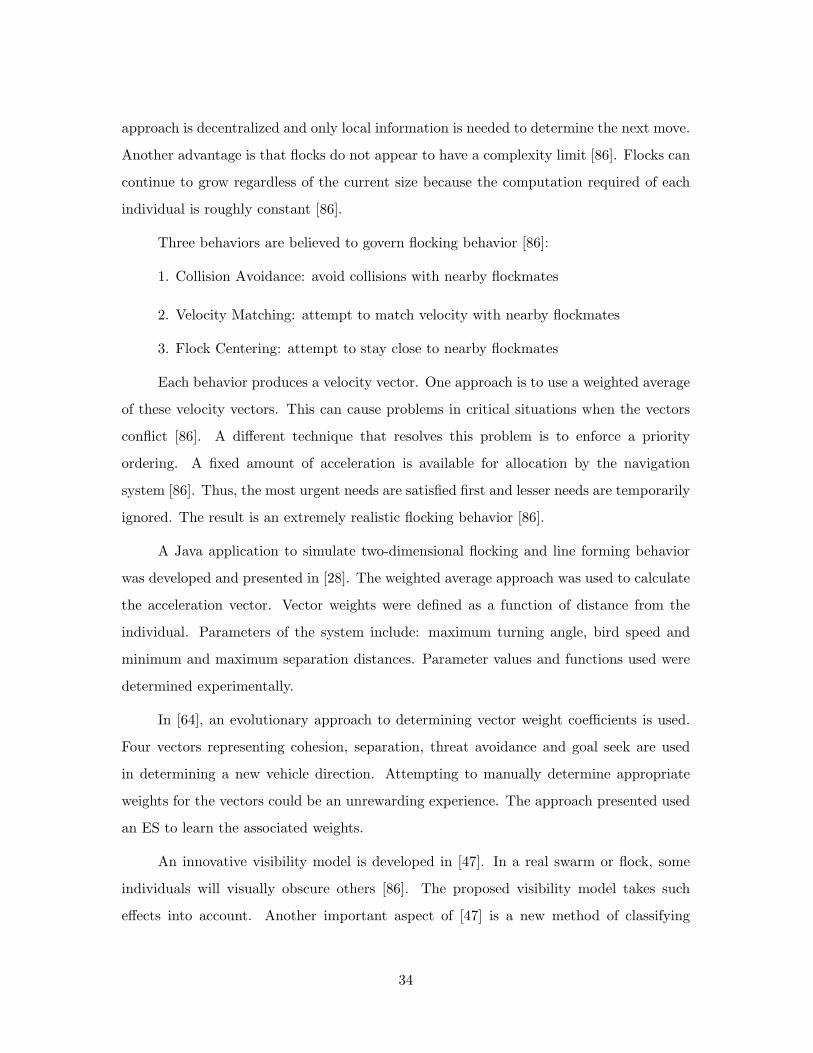
approach is decentralized and only local information is needed to determine the next move.
Another advantage is that flocks do not appear to have a complexity limit [86]. Flocks can
continue to grow regardless of the current size because the computation required of each
individual is roughly constant [86].
Three behaviors are believed to govern flocking behavior [86]:
1. Collision Avoidance: avoid collisions with nearby flockmates
2. Velocity Matching: attempt to match velocity with nearby flockmates
3. Flock Centering: attempt to stay close to nearby flockmates
Each behavior produces a velocity vector. One approach is to use a weighted average
of these velocity vectors. This can cause problems in critical situations when the vectors
conflict [86]. A different technique that resolves this problem is to enforce a priority
ordering. A fixed amount of acceleration is available for allocation by the navigation
system [86]. Thus, the most urgent needs are satisfied first and lesser needs are temporarily
ignored. The result is an extremely realistic flocking behavior [86].
A Java application to simulate two-dimensional flocking and line forming behavior
was developed and presented in [28]. The weighted average approach was used to calculate
the acceleration vector. Vector weights were defined as a function of distance from the
individual. Parameters of the system include: maximum turning angle, bird speed and
minimum and maximum separation distances. Parameter values and functions used were
determined experimentally.
In [64], an evolutionary approach to determining vector weight coefficients is used.
Four vectors representing cohesion, separation, threat avoidance and goal seek are used
in determining a new vehicle direction. Attempting to manually determine appropriate
weights for the vectors could be an unrewarding experience. The approach presented used
an ES to learn the associated weights.
An innovative visibility model is developed in [47]. In a real swarm or flock, some
individuals will visually obscure others [86]. The proposed visibility model takes such
effects into account. Another important aspect of [47] is a new method of classifying
34

swarms based on behavioral characteristics. This is a useful approach since swarm behavior
has an impact on other properties, such as communication. A chaotic swarm, similar to a
swarm of bees, is very different from a stable swarm arranged in a lattice structure. A final
area considered in [47] is swarm network communication. A link between swarm behavior
and network performance is established. Previously, no adequate method for measuring
the network performance of swarms existed.
2.3.8 Genetic Programming. Genetic programming has been used in the devel-
opment of control systems by many researchers. In [5], a GP-based system (EvoCK) is
combined with an existing learning mechanism (Hamlet) to evolve planning control rules.
Tests were performed for the blocks world and logistics domains. The combined system
produced more efficient solutions for the blocks world domain. The best solutions for the
logistics domain were produced by EvoCK alone [5]. Other approaches have used GP to
evolve plans and planners [5]. The authors state that “searching for just the heuristics is
a more feasible task” [5].
A solution to the two-dimensional pursuer/evader (2DPE) problem is presented by
Moore and Garcia [74]. In this problem a pursuer, such as a missile, chases after an
evader, like an aircraft. The pursuer is faster and more agile, but is given a limited
amount of time to reach the evader. The extended 2DPE adds simple physics (force, mass
and acceleration) to the problem [74]. The pursuer used a set method of navigation, the
proportional navigation technique [74]. Pursuers varied in mass and acceleration capability.
Evader programs were evolved against 3 pursuers, each using the static pursuer pro-
gram. Programs were evaluated using multiple scenarios with different angles of attack and
initial distances between pursuer and evader [74]. Control programs capable of successfully
evading all pursuers were evolved. When tested using a different initial distance and angle
of attack, the evolved programs were still able to evade with approximately 85% to 100%
efficiency [74]. This research shows the ability of GP to successfully deal with increases in
problem complexity. It also highlights how realistic simulations can be used to accurately
model real world situations.
35
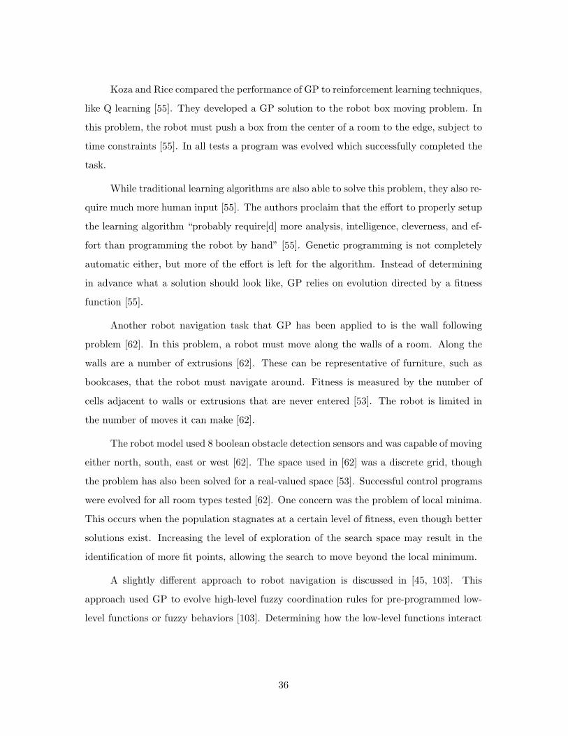
Koza and Rice compared the performance of GP to reinforcement learning techniques,
like Q learning [55]. They developed a GP solution to the robot box moving problem. In
this problem, the robot must push a box from the center of a room to the edge, subject to
time constraints [55]. In all tests a program was evolved which successfully completed the
task.
While traditional learning algorithms are also able to solve this problem, they also re-
quire much more human input [55]. The authors proclaim that the effort to properly setup
the learning algorithm “probably require[d] more analysis, intelligence, cleverness, and ef-
fort than programming the robot by hand” [55]. Genetic programming is not completely
automatic either, but more of the effort is left for the algorithm. Instead of determining
in advance what a solution should look like, GP relies on evolution directed by a fitness
function [55].
Another robot navigation task that GP has been applied to is the wall following
problem [62]. In this problem, a robot must move along the walls of a room. Along the
walls are a number of extrusions [62]. These can be representative of furniture, such as
bookcases, that the robot must navigate around. Fitness is measured by the number of
cells adjacent to walls or extrusions that are never entered [53]. The robot is limited in
the number of moves it can make [62].
The robot model used 8 boolean obstacle detection sensors and was capable of moving
either north, south, east or west [62]. The space used in [62] was a discrete grid, though
the problem has also been solved for a real-valued space [53]. Successful control programs
were evolved for all room types tested [62]. One concern was the problem of local minima.
This occurs when the population stagnates at a certain level of fitness, even though better
solutions exist. Increasing the level of exploration of the search space may result in the
identification of more fit points, allowing the search to move beyond the local minimum.
A slightly different approach to robot navigation is discussed in [45, 103]. This
approach used GP to evolve high-level fuzzy coordination rules for pre-programmed low-
level functions or fuzzy behaviors [103]. Determining how the low-level functions interact
36

to achieve a high-level behavior is “not entirely intuitive” [103] and required significant
experimentation [45].
Genetic programming was applied to discover good coordination programs without
requiring expert knowledge [45]. Results indicate that GP was able to evolve good co-
ordination strategies. The evolved coordination programs were also tested in additional
environments to determine generalizability. The strategies were moderately generalizable
[45]. This research shows how GP is able to discover complex relationships with a minimum
of human input.
Nordin and Banzhaf used GP to evolve obstacle avoidance behavior for a Khepera
robot [77]. Two architectures were examined, a memoryless and a memory-based archi-
tecture. Fitness was measured using proximity to objects and the relative and absolute
speeds of the two motors [77]. The fitness function used was:
fitness = α(m1 + m2 − |m1 −m2|)− β7∑
i=0
si (6)
with motor speeds 0 ≤ mi ≤ 15 and sensor values 0 ≤ si ≤ 1023 [77]. Higher fitness scores
were awarded for staying away from objects (low values of si) and by moving fast (high
values of mi) and in a straight line [77].
The memoryless approach used only the robot’s sensors to determine how to move.
A control function relating the sensor values and motor outputs was evolved [77]. Initially,
the robot crashed frequently, but was able to learn simple obstacle avoidance in about 10
minutes. After approximately 50 minutes of training, or 150 generation equivalents, colli-
sions were almost completely eliminated [77]. Robot behavior evolved with this approach
was chaotic, “resembl[ing] that of a bug or an ant” [77].
The second approach used a memory buffer to store vectors of sensor and motor
values [77]. This memory was used with current sensor values to determine the best move.
The memory based system was much faster at learning the obstacle avoidance behavior,
requiring only a few minutes [77]. The observed behavior was also much different than the
37

memoryless approach. Controllers evolved using memory moved in straight lines or curves
and displayed distinct obstacle avoidance strategies [77].
Reynolds explored several aspects of evolving stimulus-response controllers for agents
in a two-dimensional environment [87, 89, 88]. Reynolds notes that the evolved controllers
are “reactive agents” [87], similar to Brooks’ subsumption architecture [16]. Steady state
GP (SSGP) was used in all of the experiments. Sensor capabilities are evolved along
with control. Manually specifying sensor placement could influence the type of strategies
evolved [89]. Constant forward motion is used in all experiments.
In [87], a controller for a group of “critters” is evolved. They must avoid collisions
with one another, obstacles in the environment and a roaming predator. Each controller is
limited to information about the world which is accessible through its sensors. Using this
“foggy world” perception model, objects are detected with an intensity inversely propor-
tional to the square of their distance from the observer [87]. Objects are also obscured by
other objects between them and the sensors.
Robustness of solutions was considered [87]. The solution used was to use random
starting positions and orientations for the critters and predator. Each controller was
tested using two different starting points. Increasingly robust behavior may be achieved
by increasing the skill of the predator [87]. This could be achieved through coevolution of
the predator and critters [87].
The only action available to the critters is turning in a specified direction. Even
with the limited sensor and movement capabilities, complex reactive behavior was evolved
[87]. One improvement identified for the model was the ability to sense, in addition to
proximity, the direction of movement for other critters or the predator [87]. The evolution
of improved grouping behavior is in need of additional research [87].
In [89], the focus is vision-based obstacle avoidance. Only single critters were consid-
ered. Critters were evaluated based on how long they survived while maneuvering through
an environment with obstacles. Two experiments were performed, one using a single fit-
ness trial and one using three trials with different starting locations. The first experiment
produced individuals three times more fit than those in the second experiment. This per-
38

formance decrease is tentatively attributed to the increased complexity required to evolve
generalized controllers, though additional insight is needed [89].
Reynolds also looked at the evolution of corridor following behavior [88]. Again, only
a single critter is considered. Emphasis is placed on developing non-brittle solutions that
are able to perform effectively in diverse environments. An important distinction is made
between the “ ‘steering’ and ‘path determination’” approaches being considered and “path
planning” [88]. The evolved controllers rely on sensor inputs to determine appropriate
actions, not predetermined plans.
A novel approach to the generalization problem is taken. When a critter successfully
navigates a corridor, it is tested on a different corridor. Sixteen different corridors were
used. This approach ensures that controllers to successfully navigate one corridor are
evolved before attempting to generalize them [88]. Although the desired behavior was
evolved, questions of robustness and reliability have not been satisfactorily resolved [88].
This remains an open issue for GP.
In contrast to the reactive programs generated by Reynolds, Andre evolved programs
that created a model of their environment [6]. Operating in a two-dimensional grid world,
the objective of the MAPMAKER system was to collect gold. The system was composed
of two co-evolved programs: map maker and map user. The map maker used sensor
information about the environment to create a map which the map user used to locate the
gold. Coordination between the two programs was essential to accomplishing the task [6].
A simple memory system was also used in [40]. The experiment considered a two-
dimensional grid world filled with explosives and energy. Agents were able to maintain
a list of cells they had already visited. Experiments with one agent and multiple agents
were performed. Robust solutions were developed by using a different map for each new
generation.
Genetic programming has also been used to evolve control programs for multiple
predators in predator/prey systems [39, 69]. Haynes et al., compare an evolved solution to
previous hand-coded efforts [39]. The simulated environment was a two-dimensional grid
world with four homogenous predators and a single prey. Predators were not given explicit
39

communication abilities. Strategies competitive with the best deterministic algorithms
were evolved [39]. The lack of explicit communication between predators was an identified
weakness of the work [39].
Luke and Spector examined teamwork and coordination in the predator/prey model
[69]. They considered a real-valued two-dimensional space. Two aspects reviewed were
“breeding” and sensing capabilities. Breeding was a concern for experiments where each
predator used a separately evolved controller. Restricted breeding is similar to the island
model [10]. Separate populations exist for each controller. With the free breeding model,
a single population is used, but different individuals are selected to form the team [69].
Three different forms of communication were tested: no-sensing, deictic and name-
based sensing [69]. Deictic sensing provides limited information about the current location
of other predators. A vector pointing toward the nearest predator is an example of deictic
sensing. With name-based sensing, predators are explicitly identified.
When no sensing was used, homogenous predators performed the best [69]. In ex-
periments with name-based sensing, heterogeneous individuals dominated. In all cases,
restricted breeding outperformed free breeding. Even though heterogeneous teams per-
formed the best with name based sensing, there is some concern about whether the in-
crease in performance is justified by the additional computation required [69]. Allowing the
evolution of explicit communication between agents is offered as an area of future research
[69].
The difficulty of generating robust robot control programs was considered by Ito [44]
and Chongstitvatana [23]. Ito states that, “the more the evolutionary process proceeds, the
more the genes adapt heavily to the training environment” [44]. As a result, small changes
in the environment can render the evolved controllers useless [44, 23]. Though robustness
is considered a requirement for performing real world tasks, it is often neglected in the
research [44].
There are two types of robustness to consider [44]. Individual robustness measures
the ability of evolved solutions to adapt to new or modified environments. Using a different
40

starting location or orientation and adding noise to sensors and actuators are techniques
proposed to improve individual robustness [23, 39, 44, 88].
Population robustness is the ability of the “genetic pool” [44] to continue evolving
after the environment is changed [44]. Experiments by Ito revealed that GP was able to
evolve controllers for the new environment when changed during evolution [44]. The new
solution was not robust though, as it failed to work for the initial environment. Good
solutions were evolved in fewer generations, suggesting that effective building blocks were
present in the population [44].
Robust obstacle avoidance behavior is evolved in [23] by evaluating each individual
in multiple, similar environments. More robust programs were generated when a large
number of very similar environments was used in the fitness evaluation. Decreasing the
similarity or number of environments produced less robust solutions [23].
The emergence of collective behavior in flying agents has recently been examined
[97]. Simulations were performed in a three-dimensional, real-valued environment. Two
experiments were presented in which agents had to obtain energy from randomly located
energy sources. The first extended Reynolds’ work on flocking [86], allowing for multiple
species, goal seeking behavior and evolution of the coefficients in the “motion control equa-
tion” [97]. Reproduction occurred when an individual ran out of energy. The genome of
the best individual of the same species, possibly mutated, was used for the new individual.
A complex, energy guarding behavior often emerged in the simulations [97].
The second experiment evolved control programs using GP [97]. For this experiment,
the distinction between species was removed and agents were allowed to transfer energy to
each other. Evolution was “autoconstructive” which means that individuals are responsible
for their own reproduction [97]. Again, complex behaviors, such as the “altruistic feed-
ing behavior,” were observed. This research illustrates the ability to evolve coordinated
behavior in a three-dimensional environment.
41

2.4 Summary
This chapter presented the historical origins of genetic programming and its relation-
ship to other approaches used in evolutionary computation. A general description of the
problem domain was provided. A survey of autonomous agent control systems was also
performed. Evolutionary and non-evolutionary approaches were reviewed and compared.
In Chapter 3, the existing research is used to guide the development of a high level system
design.
42

3. High Level System Design
3.1 Introduction
There are many important aspects of algorithm selection and design. This chapter
provides a detailed examination of the problem domain and its relationship to the selected
algorithm domain. First, important environmental characteristics are discussed. Then, a
description of the vehicle model is given, including sensors and communications. Next,
the algorithmic approach used is presented along with a mapping between the algorithm
domain and problem domain. Finally, the value of visualization and solid software engi-
neering principles are reviewed.
3.2 Simulated Environment
The environment being considered has a significant impact on the remaining aspects
of the problem. A discrete, two-dimensional grid world environment has a much lower
complexity than a real-valued, three-dimensional environment. Reducing the complexity
is sometimes an effective means of gaining insight into a problem. It may also be necessary
to make simplifying assumptions in order to make the problem manageable.
Solutions produced using over-simplified models may be of little value in solving the
original problem. Many efforts that work well in simulation fail to scale when implemented
in the real world [21, 38]. When simulation must be used, due to practicality, safety or
other concerns, it should be as realistic as possible.
The research presented in this thesis considers a three-dimensional environment.
Much of the existing research on evolved swarm behavior deals only with the two-dimen-
sional case [28, 47, 64, 101]. This restriction corresponds to flight restricted to a plane,
which is typically how real vehicles are flown. The restriction also carries with it an
implicit assumption that level flight is the best way to perform the given missions. It is
not intuitively obvious that that is the case.
Many different types of objects exist inside the environment (E). The most impor-
tant for this project are the set of vehicles, (V). The vehicle model is presented in the
next section. Also present in the environment are threat regions (T), obstructions (O),
43

waypoints (W) and goals or targets (G). Refer to Section 2.2 for further details regarding
notation.
Given a point, p ∈ E, it is important to know if p ∈ γ, where γ is an arbitrary region.
Regions are used to represent any volume in the environment. The scope of a vehicle’s
sensor or communication equipment, the volume covered by enemy radar and restricted
airspace are all examples of regions. It is possible to define a function gγ() such that:
gγ(p, τ) > 0 if p is outside of region γ at time τ (7)
gγ(p, τ) = 0 if p is on the surface of γ at time τ
gγ(p, τ) < 0 if p is inside region γ at time τ
∀π ∀τ ∃p s.t. gγ1(p, τ) 6= gγ2(π(p, τ)) (8)
γ1, γ2 ∈ Γ
where π is a function to convert points (using translation and rotation [33]) to a common
frame of reference and Γ is the set of all regions.
Two regions are only equal iff they always have the same shape, at the same time.
Each region may have a unique shape. For instance, one type of sensor may cover a wide
angle with a limited range, while another covers a narrow angle but with a long range.
Both of these regions would differ from a region representing an obstacle like a tree or
mountain.
The shape of regions is also allowed to vary with time. This could represent a change
in the power of a radar or in the direction of a sensor. Note that the choice of coordinate
systems is arbitrary. There are well known equations to convert between rectangular,
cylindrical and spherical coordinate systems [7].
A complete physics model allows the implementation of Newton’s second law: F =
ma. This allows the inclusion of friction, gravity and aerodynamic forces to the model
[101]. Once these forces are calculated, they can be used to determine fuel or energy
requirements. Simulating the effects of physical forces can significantly increase the com-
putational requirements of a system [50, 74].
44

Few researchers appear to have explored the consequences of an accurate physics
model. Trahan et al., implemented a two-dimensional swarm model using particle physics
[101]. Moore and Garcia extended the two-dimensional pursuer/evader problem by adding
mass to the system [74]. Certainly if realism is a goal, accurate physics should be included
in the simulation wherever possible.
Another aspect of an environment is whether it is static or dynamic. In a static
environment, regions do not change with time:
∀i, j gγ(p, τi) = gγ(p, τj) (9)
Static environments are computationally less demanding, since fewer aspects of the en-
vironment must be monitored and updated. They also have less realism than dynamic
environments. In real world scenarios, threats and targets may be mobile [65]. Such prob-
lems are likely to require cooperation and coordination among teammates to be solved
effectively [39, 69].
3.3 Vehicle Model
The vehicle model is the central model in the simulation. A vehicle can be defined by
its sensor, movement and communications capabilities. Vehicles can either be homogenous
or heterogeneous. Recent swarm research has focused on the homogenous vehicle model
[47, 64]. The control, capabilities and composition of vehicles in the swarm ultimately
determines its behavior. Reynolds’ study of bird flocking behavior provides an example of
this [86].
One approach to designing a vehicle model comes from the field of control theory
[45]. Figure 9 illustrates a simple control system. The plant is the object under control. In
this thesis, the plant is a single UAV. Each vehicle has a controller that accepts input from
sensors. Information about the environment and current state of the plant is combined
to produce a control signal. The control signal directs the plant. The plant may also be
affected by other forces, such as gravity.
45

Figure 9 High level system control diagram [45]
The goal of this research is to produce an effective control system for a swarm of
UAVs. Using techniques from evolutionary computation, specifically genetic programming,
a control program is evolved to direct the movements of the UAVs. In general, there may
be many different types of vehicles, each with their own unique controller. The set of
vehicles using controller Cx is denoted as Vx. In this project, only homogenous sets of
vehicles are considered, thus Vx = V .
Some of the properties that vehicles in the simulation have are: position, speed,
heading. Vehicles also have certain movement constraints which are discussed in Section
3.3.1. In general, vehicles can have a local or global frame of reference, or both [64].
In a local frame of reference, all values are given relative to one’s current location and
heading. In contrast, a global frame of reference uses absolute values common throughout
the environment.
Consider the command TURN 30. Using a local frame of reference, it means turn
right 30 degrees. When using a global frame of reference though, the same instruction
means to make the new heading 30 degrees. The use of a global coordinate system relies
on the ability to obtain coordinates from some system, such as the global positioning
system (GPS) [64]. It does not seem unreasonable to assume, for purposes of this research,
that such a system will be available.
46
Constraints (R)
Sensors (S) Controller
Effects (v.)
Plant
Control Signal (v)
Feedback

Figure 10 Visual depiction of vectors and actuator constraints associated with vehiclemovement
Physicals quantities with numerical and directional components can be representing
using vectors [91]. Force, acceleration, velocity and displacement can all be represented
using vectors. These are precisely the values that are of concern in controlling a vehicle.
The combination of thrust and steering forces act on an aircraft to produce motion in
a certain direction, called velocity. Equations used for calculating these values are well
known.
To illustrate the use of vectors used in this research, consider the following example,
depicted in figure 10. A vehicle v is at a location, or displacement, vr0 and is attempting
to reach a different point, vr1. A new vector from the current position to the destination
can be calculated by subtracting: vr1−vr0 . This value is the new desired velocity, vv1 . An
acceleration is applied so that the vehicle will attain the new velocity: vva = 2(vv1 −vv0).
3.3.1 Sensors. Vehicles gather information about their environment from sensors.
One approach to sensor models is based on vision [47, 64, 86, 87, 89]. A sensor is used to
scan an area around the vehicle. The sensors may be able to detect, identify and determine
the distances to objects [87]. Though actual vision-based sensors may be used, often the
sensors under consideration are somewhat simplified [55, 62, 77]. The Khepera robot, for
instance, uses 8 infrared proximity sensors [77].
47
max
/ran
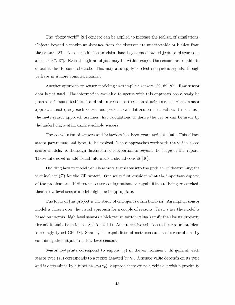
The “foggy world” [87] concept can be applied to increase the realism of simulations.
Objects beyond a maximum distance from the observer are undetectable or hidden from
the sensors [87]. Another addition to vision-based systems allows objects to obscure one
another [47, 87]. Even though an object may be within range, the sensors are unable to
detect it due to some obstacle. This may also apply to electromagnetic signals, though
perhaps in a more complex manner.
Another approach to sensor modeling uses implicit sensors [39, 69, 97]. Raw sensor
data is not used. The information available to agents with this approach has already be
processed in some fashion. To obtain a vector to the nearest neighbor, the visual sensor
approach must query each sensor and perform calculations on their values. In contrast,
the meta-sensor approach assumes that calculations to derive the vector can be made by
the underlying system using available sensors.
The coevolution of sensors and behaviors has been examined [18, 106]. This allows
sensor parameters and types to be evolved. These approaches work with the vision-based
sensor models. A thorough discussion of coevolution is beyond the scope of this report.
Those interested in additional information should consult [10].
Deciding how to model vehicle sensors translates into the problem of determining the
terminal set (T ) for the GP system. One must first consider what the important aspects
of the problem are. If different sensor configurations or capabilities are being researched,
then a low level sensor model might be inappropriate.
The focus of this project is the study of emergent swarm behavior. An implicit sensor
model is chosen over the visual approach for a couple of reasons. First, since the model is
based on vectors, high level sensors which return vector values satisfy the closure property
(for additional discussion see Section 4.1.1). An alternative solution to the closure problem
is strongly typed GP [73]. Second, the capabilities of meta-sensors can be reproduced by
combining the output from low level sensors.
Sensor footprints correspond to regions (γ) in the environment. In general, each
sensor type (sx) corresponds to a region denoted by γx. A sensor value depends on its type
and is determined by a function, σx(γx). Suppose there exists a vehicle v with a proximity
48

sensor σi as described in [87]. The sensor value P can be calculated using the following:
P = σp(πv(γp)) (10)
γp : y = x where 1 < x ≤ 15
πv : A transformation function which shifts γp to v’s frame of reference
σp =
1x2 where x is the minimum distance before another region intersects γp
0 otherwise
A biologically inspired vision approach may use one or two, conic or parabolic regions.
The sensor function could reduce the accuracy for points near the edges of the region(s)
to simulate peripheral vision [47, 64]. Other approaches might use many different sensors.
Their locations and types could be decided a priori or evolved [106].
A single, spherical sensor region γs is used in the current project. The radius of the
sphere defines a vehicle’s neighborhood, N . Only events which occur within this region can
be sensed by an individual. Events occurring beyond the neighborhood require external
communication.
Two meta-sensors are used: getV elocity(i) and getPosition(i). Each function re-
turns the value pertaining to the ith closest neighbor and itself when i = 0. A vehicle
can calculate positional information for its neighbors using a distance sensor and its own
position and orientation. The orientation of one’s neighbors could be determined using
visual cues [87]. Unfortunately, this does not accurately account for shadowing effects [47].
Each vehicle could localcast its identifier, position and orientation.
Accurately determining a neighbor’s velocity is a more difficult task. The previous
position and orientation of all neighbors can be maintained. In order to compare val-
ues, some method of identifying individuals is also required. Alternatively, each vehicle
could perform a local broadcast including its current velocity. The feasibility of such a
communication scheme seems questionable, but still plausible.
Neighbors can be any sense-able object including, but not limited to: friendly ve-
hicles, enemy vehicles, obstacles and targets. The three sensor capabilities used in this
research are: getPosition(i), getV elocity(i) and identify. The identify function repre-
49

sents a set of boolean identification functions, such as the friend(i) function described
below. These sensors are sufficient for developing flocking behavior [86].
Collision Avoidance : vvavoid =1j
j∑i=1
(getPosition(0)− getPosition(i)) (11)
where |getPosition(0)− getPosition(j)| ≤ dmin
Velocity Matching : vvmatch =1n
n∑i=1
(getV elocity(i) · friend(i)) (12)
where n = |N | and friend(i) = 1 if the ith nearest neighbor is a
friendly vehicle and 0 otherwise
Flock Centering : vvcenter =1
n− k + 1
n∑i=(k)
(getPosition(0)− getPosition(i))(13)
where |getPosition(0)− getPosition(k)| > dcomfort
vvnew = ωcavvavoid + ωvmvvmatch + ωfcvvcenter (14)
where ω represents the weight of each vector in determining the new velocity [28, 86, 97].
3.3.2 Actuators. Actuators provide the physical instantiation of signals generated
by the controller. Different actuators on aircraft include: the engine, slats, spoiler, aileron,
flaps, elevator and rudder [22]. The state of these controls, along with physical forces
acting on the aircraft, determine its motion.
Evolved control programs produce control signal values that are translated to actions.
Nordin and Banzhaf used evolved programs to determine motor speed values for a Khepera
robot [77]. Koza and Rice evolved a robot control program using three movements: turn
right 30 degrees, turn left 30 degrees and move forward 1/3 foot [55]. Reynolds’ systems
calculated turn angles for critters with constant forward movement [87, 89, 88]. Systems
producing vector values for control were described in [69] and [97].
Accurately simulation must include simulating the real limitations of objects. An op-
timal course of action may not actually be possible due to real world constraints. Changing
an aircraft’s heading 180 degrees in 1 second may be desirable if a collision is about to
occur. However, it also violates the maneuvering capabilities of known aircraft.
50

Two approaches to dealing with infeasible solutions are to generate only feasible
solutions or to fix the infeasible solutions. One approach at guaranteeing feasible solutions
is to restrict the set of functions and terminals. Consider the function TURN θ with the
restriction that θ ≤ 30. This would involve defining a set of functions and terminals so
that θ will never be assigned a value greater than 30.
Another method is to use specialized genetic operators [9, 73]. This is how strongly
typed genetic programming works. A special type, A, is defined for θ. Then, only terminals
of type A and functions returning type A are allowed as arguments to the TURN function.
Alternatively, invalid solutions can be altered so that they no longer violate the
problem constraints. Values that are too large can be reduced to an acceptable size [87].
Suppose θ = 87. The TURN function could substitute 30. This is the approach used in
here.
There are several constraints associated with vehicles: minimum (vvmin) and max-
imum velocity (vvmax), maximum acceleration (vamax) and maximum turn rate (θmax).
These values are determined by physical capabilities of the vehicle. A function can be
defined to adjust the desired velocity so that all constraints are satisfied:
ζ(vv1) = vv2 s.t. vvmin ≤ vv2 ≤ vvmax (15)
2(vv2 − vv0) ≤ vamax
arccos(
vv0 · vv2
|vv0 ||vv2 |
)≤ θmax
3.3.3 Communications. Communication between agents is another aspect to be
considered when designing multi-agent systems. Some method of communication is needed
to allow two or more agents to coordinate their actions. If one agent locates a threat or
target, the other agents in the system would benefit from sharing in that knowledge.
Communication in a dynamic, distributed system is a complex problem that has recently
been explored by Kadrovach [47].
There are two board types of communication: explicit and implicit. Explicit commu-
nication includes direct, agent-to-agent messaging as well as broadcast messages. As the
51

number of agents in the system grows, the amount of communication between agents also
grows [47, 64]. Since bandwidth is limited, efficient methods of allocating it are desired.
Reliance on explicit communication is a potential risk for a distributed system devel-
oped for use in hostile environments. Systems using a hierarchical communication system
are efficient, but highly vulnerable to disruption [26]. Even systems using decentralized
communications are subject to jamming or possibly the need for silent operation.
One solution to the problems of explicit communication is based on stigmergy. “Two
individuals interact indirectly when one of then modifies the environment and the other
responds to the new environment at a later time. Such an interaction is an example of
stigmergy” [15]. The use of pheromones by ants is an example of stigmergy. The idea of
artificial pheromones has been used to develop simulated swarm control systems [36].
Implicit communication uses vehicles’ sensor values in conjunction with some decision
function to make navigation decisions. The sensors used are not directly implementable and
would likely require inter-agent communication. This is a common technique in research on
multi-agent coordination [64, 69, 87, 89, 97]. Luke and Spector showed that evolved teams
of homogeneous agents (using the same controller) using implicit communication were
unable to increase performance when direct, agent-to-agent communication was available
[69]. Heterogeneous teams however, were able to increase performance with the increased
communication capability.
Another aspect to consider is the range of communication. Long range communi-
cation requires greater transmission power than local communication. This is a concern
for a micro-UAV with a very limited power capacity. Given a vehicle (v), the set of vehi-
cles within communication range is called its neighborhood, N . In Section 3.3.1 this was
defined as a spherical region, γs. In general, different neighborhoods could be defined by
considering the elements of the power set of all sensor (including communication sensors)
regions.
Nz | z ∈ P(ΓS) (16)
The size of a neighborhood is an important property of swarm systems. Global com-
munications produces the largest possible neighborhood, where all individuals are neigh-
52

bors. Each individual must consider all others, resulting in a computational complexity of
O(n2) [50, 64, 86]. For a few dozen members this is fine, but when working with hundreds
or thousands of individuals it quickly becomes unacceptable.
The opposite extreme, a very small neighborhood, can also cause problems. Individ-
uals may lose contact with the swarm if the neighborhood size is too small. Cooperative
behavior is prevented from emerging since individuals have severely limited interactions
with one another. Neighborhood size is often specified as a system parameter, though
there is no reason it has to be static.
This project does not directly consider the communication layer. Explicit commu-
nication is not used. Two scenarios are studied. The first uses getVelocity sensors which
are assumed to require some undefined form of communication. The second scenario uses
only getPosition sensors which are assumed to require no communication.
3.4 Mapping to Genetic Programming
The method used to generate controllers for the UAV swarm simulations is genetic
programming. Genetic programming allows the evolution of entire controllers, not just the
parameters as is the case with other EA approaches [64]. Novel controllers can be developed
that take into account aspects of the problem not previously considered by human experts.
All one must do is provide the GP system with the pieces needed to assemble a good
solution.
That said, evolutionary computation, and genetic programming in particular, is not
a panacea. Evolution exploits easy to find solutions even if they’re the result of an error in
the problem specification [39]. Careful consideration must be given to the definition of the
evolutionary environment. In this section a general design methodology is presented. A
high level mapping between of the autonomous UAV swarm control problem to the genetic
programming domain is given. The specific details of implementation are presented in
Chapter 4.
To fully map a problem into the GP algorithm domain, five things must be specified:
the terminal set, function set, fitness function, parameters in the problem and algorithm
53

domains and termination criteria [53]. There are many different possible mappings for a
given problem domain. Consideration is given to these alternatives.
The terminal symbols (T ) correspond to leaf nodes in evolved program trees. There
are two often used approaches to designing the terminal set. First, terminals can return
values. The terminal five may return the numerical value of 5. A terminal could be used
to represent the current value returned by a sensor [55, 62, 69].
Second, terminals may have side-effects. That is, when evaluated they cause some
action to be performed in addition to, or instead of, returning a value. The terminal set
for the artificial ant problem is: turn right, turn left, move forward [53]. Each terminal
causes the ant to perform the associated action without returning a value to the parent
node.
The terminal set chosen for this project has no side-effects. Each terminal represents
sensor information that can either be directly observed or calculated using information from
sensors and communication with other vehicles. By defining T in this way, the relationship
between the sensors and terminals is emphasized. The use of side-effects appears limited
to situations where only a finite number of possible actions exist [23, 53, 55, 62].
The set of functions (F) operate on the values returned by terminal symbols and
other functions. They form the interior nodes of the program tree. Functions have one
or more arguments and return a single value. The set of functions used must be closed:
∀x∃y s.t. y = f(x). This can be satisfied by designing each function so that it can handle
all possible argument types or through restrictions on genetic operators, as in STGP [73].
Like terminal symbols, functions can also have an effect on the simulation [40, 87, 97].
An example of this is the function TURN θ which causes a vehicle’s heading to be modified
by the angle θ. Another type of function is a combination operator. The arithmetic
operators are examples of this. There are also control functions, like IF-THEN x y z,
which provide a means of conditional execution. For instance, if a vehicle is too close to
an obstacle then take corrective action; otherwise perform the standard action.
The functions used in this project are all combination functions. Vector manipulation
functions are used to produce a controller, C(), that converts sensor values into a new target
54

velocity:
targetV elocity = C(s1, s2, ..., sn) (17)
All functions used in this project are of the combination class. Allowing side-effects blurs
the line between sensors, actuators and control. Control functions have been excluded in
order to keep problem complexity to a minimum. This examination provides a baseline or
benchmark from which to measure future progress.
Of prime importance in any evolutionary algorithm is the fitness function. It is the
fitness function that provides the evolutionary force which drives the search for solutions
[9]. Individuals with good building blocks, subtrees in GP, should be identified by the
fitness function. These more fit individuals are given a higher probability of reproduction.
In this way, good building blocks are propagated throughout the population.
Good partial solutions are combined to form good problem solutions. Some properties
of good solutions identified for the current problem are: no crashing into other swarm
members, no crashing into objects, avoiding threat regions, reaching the assigned targets
and moving as a group (exhibiting a natural flocking behavior).
Objective functions generate a numerical value measuring the performance of an
individual with respect to certain attributes [9]:
f : αi → R (18)
Consider the objective: Minimize the number of crashes. This can be represented symbol-
ically as:
f1 = minn∑
i=0
(crashedi) (19)
55

where crashedi = 1 if vehicle i crashed and 0 otherwise. In addition to equation 19, three
other objective functions were defined:
f2 = max|G|∑k=0
n∑i=0
(reachedTargeti(k)) (20)
f3 = minτend∑τ=0
n∑i=0
(centerDisti(τ)) (21)
f4 = minτend∑τ=0
n∑i=0
(targetDisti(τ)) (22)
where reachedTargeti(k) > 0 if vehicle i has reached target k and 0 otherwise. The
distance functions, centerDisti(τ) and targetDisti(τ) return the distance at time τ , from
vehicle i to the swarm center of mass and current target of vehicle i respectively.
The fitness function combines objective functions to produce an overall fitness for
each individual [9]. The plain aggregating approach to multiobjective optimization is used
for this project [10]. This can be represented as follows:
F : Rn → R (23)
F =n∑
k=1
(ωk fk(αi)) (24)
where ωk is the weight given to objective k. Further discussion of fitness functions can be
found in Section 4.1.2.
The final aspect to consider when using GP to solve a problem is the system con-
figuration. Some problems may require, or benefit from, the use of unique genetic opera-
tors. Specialized operators to reduce the size of solutions have been proposed [14, 57, 67].
Additional operators have been proposed to improve search effectiveness by increasing ex-
ploration [84] and exploitation [80]. No new operators have been implemented for this
project.
The genetic operators used in this project are the standard GP operators defined
in [53]: reproduction, crossover and mutation. Ramped half-and-half initialization is per-
formed and a strict depth limit is enforced for all trees. Although initial GP efforts focused
56

on fitness proportionate selection [53], tournament selection is now the dominant method
in use [6, 62, 69, 87]. Further details such as population size and specific parameter values
are provided in Chapters 4 and 5.
3.5 Visualization
Having a lot of data is of no use unless it can be translated into useful information.
The output of a GP system is a program tree. For some problems, like symbolic regression,
that is sufficient to describe the solution. It is difficult to determine the behavior of a
controller in an environment simply by examining the program tree. This problem becomes
exponentially more complex when additional vehicles are added. One way to solve this
problem is through some type of visualization software.
The visualization tool used must be able to replicate the simulated environment in
which controllers are evolved. This means that a three-dimensional environment must be
supported. Objects in that environment, threats and targets for instance, must also be
supported. The ease of integrating the evolved controller into the visualization environment
is another concern. Having a way to automatically import controllers into the visualization
environment would be ideal.
A solution to both concerns is to use the same system for visualization and simulation.
There are many simulation systems available that are capable of modeling UAV swarms
[25]. Icosystem Corporation produced a swarm simulator called Simulation [25, 36]. It was
developed under contract for the Air Force Research Labs. The MultiUAV simulator also
supports a three-dimensional environment. Scalability is limited though, and additional
software (Matlab and Simulink) is required to run the system [25]. Another system was
used by Spector et al., in recent efforts at simulating behavior of flying agents [97]. Breve
is a three-dimensional simulation environment “designed for simulation of decentralized
systems and artificial life” [50]. Specific software selections are presented in Section 4.2.
57

3.6 Software Engineering Principles
Modularity and code reuse are two principles of good software design [94]. There
is no point in reinventing the wheel. Reusing existing functions, modules or sub-systems
can dramatically reduce the time and effort required to produce a system. Furthermore,
existing software is likely to be more reliable, having already “been tested in operational
systems” [94]. Unfortunately, unique requirements sometimes do not allow for reuse. Inte-
grating existing software into one’s system may also require more effort than implementing
the same functionality from scratch.
Designing a system with modularity in mind can enable the reuse of components and
simplify testing and integration [94]. A flexible system architecture is essential in enabling
efficient, continuing research. In loosely coupled systems, modules can be swapped with
other functionally equivalent modules to study their impact. An excellent example of this
would be genetic operators in an EC system. Using modular design, new genetic operators
can be designed, implemented and studied with minimal effort.
These principles guided the development of the the system used in this project. Three
main sub-systems were identified: the GP system, a simulation and visualization environ-
ment and a conversion utility. Different GP platforms and possibly different visualization
systems could be applied to this architecture. The potential also exists to apply evolved
control programs to real robots. Cazangi et al., showed that control systems evolved in a
simulated environment can be successfully applied to a physical environment [21].
3.7 Summary
The high level design was presented in this chapter. This includes models of the
environment and vehicles including sensors, actuators and communications. A general
mapping of the problem domain into the genetic programming algorithm domain was also
given. Visualization requirements and software engineering principles were reviewed. The
next chapter uses this high level design to produce a low level specification and describes
the system implementation.
58

4. Low Level Design and Implementation
This chapter presents the low level design and details of implementation. First, the high
level design and mappings presented in Chapter 3 are refined into a low level specification.
The function and terminal sets, fitness functions and system parameters are completely de-
fined. Then, the final system architecture, including existing and newly developed software
packages, is described. Finally, system implementation details are provided.
4.1 Low Level Design
A low level design specification provides all of the details required to fully implement
a system. This section refines the high level GP design from the previous chapter. All
function and terminal symbols are defined. Next, the objective functions are combined to
produce a fitness function. Finally, a comprehensive list of system parameters for the GP
system and simulation model, along with their default values, is presented.
4.1.1 Terminals and Functions. The complete set of terminals for this project
represents a variety of derived sensor values. Each terminal is listed here, followed by its
symbolic definition and a narrative description. Terminals can be calculated as displace-
ments from the origin (r) and/or as velocities (v). A rectangular coordinate system is
used.
myCurV elocity [v] : curV elocity(0)
A vector of the vehicle’s velocity.
getAvgV elocity [v] : 1n
∑ni=1(getV elocity(i) · friend(i))
A vector of the average velocity of friends in the neighborhood.
myCurPosition [r] : curPosition(0)
A vector to the vehicle’s position.
getCenterNeighbors [r, v] : 1n
∑ni=1(getPosition(i) · friend(i))− getPosition(0)
A vector to the average position of friends in the neighborhood.
getTargetPosition [r, v] : getTarget(i) where i is the vehicle’s current target
A vector to the vehicle’s current target.
59

myClosestNeighbor [r, v] : (nearestNeighbor − getPosition(0)) where
nearestNeighbor = getPosition(i) if ∃i∀(j < i) (friend(i) = 1 and
friend(j) = 0) otherwise zeroV ector
A vector to the closest friend in the neighborhood.
getClosestObstacle [r, v] : (nearestObstacle− getPosition(0) where
nearestObstacle = getPosition(i) if ∃i∀(j < i) (obstacle(i) = 1 and
obstacle(j) = 0) otherwise zeroV ector
A vector to the closest obstacle in the neighborhood.
∗ getAwayV ector [v] : getPosition(0)−1n
∑ni=1 (getPosition(i) · friend(i) · tooClose(i)) where tooClose(i) = 1
if (getPosition(i)− getPosition(0) ≤ rcrowded and 0 otherwise
A vector away from friends that are too close (defined by distance rcrowded).
∗ getCloserV ector [v] : 1n
∑ni=1 (getPosition(i) · friend(i) · tooFar(i))−
getPosition(0) where tooFar(i) = 1
if (getPosition(i)− getPosition(0) ≥ risolated and 0 otherwise
A vector toward friends that are too far away (defined by distance risolated
∗ getAvgHeading [v] : 1n
∑ni=1(getHeading(i) · friend(i))
unitV ector[v] : returns the vector (1, 1, 1).
doubleV ector[v] : returns the vector (2, 2, 2).
All functions used are mathematical vector operations. They apply equally to dis-
placements, velocities and accelerations. The evolved control programs produce a new
velocity vector by combining different sensor values represented in the terminal set.
vAdd(v1, v2) : Returns the result of adding v1 and v2.
vSub(v1, v2) : Returns the result of subtracting v2 from v1.
vMult(v1, v2) : Returns the result of multiplying v1 by |v2|.
vDiv(v2, v2) : Returns the result of dividing v1 by |v2|.
vCross(v1, v2) : Returns the cross product of v1 and v2 (specifically, v1× v2).
60

∗ normalize(v1) : Returns the normalized vector of v1 (v1/|v1|).
NOTE: Instructions and functions marked with an asterisk were designed, but not
fully implemented.
The key factors in choosing the sets T and F are the requirements for closure and
satisfiability [53]. Closure is satisfied by selecting vectors for the terminals and vector
operations for the functions. The multiplication and division operators, which normally
use a vector and a scalar value, were redefined to use two vector arguments.
An alternative approach to closure is strongly typed genetic programming (STGP)
[73]. Using STGP, function arguments are automatically matched with compatible types.
The use of vector values seemed like a natural approach and satisfied all requirements,
so STGP was not implemented. Future approaches using scalar values could benefit from
strong typing.
Satisfiability is the other major requirement that must be met. The primitives used
in this project are similar to those used in non-GP related work [28, 47, 64, 86]. As
illustrated by equations 11 - 14 in Section 3.3.1, the sensor model is sufficient for producing
coordinated group behavior. Since solutions to the problem can be represented using the
sets defined, the requirement of satisfiability has been met.
4.1.2 Fitness Functions. Instead of evolving weight coefficients for an existing
equation, the proposed GP system generates an entirely new equation. The resulting con-
trol programs are evaluated based on certain objectives. Four different objectives functions
were given in Section 3.4. Each objective function defined a specific desirable characteristic
of the emergent swarm behavior: avoid crashing, stay in a close group and move toward the
assigned targets. The fourth objective function encourages individuals to actually reach
the assigned target.
61

The final fitness function, which was developed through experimentation, is:
F =
(τend∑τ=0
n∑i=0
(centerDist(i, τ)) +τend∑τ=0
n∑i=0
(targetDist(i, τ)) + CP
)·(n · |G|)−
(∑|G|k=0
∑ni=0 (reachedTarget(i, k))
)(n · |G|+ 1.0)
(25)
CP = β ·
n∑i=0
τend∑τcrash
|G|∑i=0
|targetPosition(i + 1)− targetPosition(i)|
(26)
where n is the number of vehicles, |G| is the number of targets, τ is the simulation time
and β is a weight for the crash penalty function.
The first term calculates the sum of the average distance of each vehicle from the
swarm center of mass over the allotted time. The second term calculates the total distance
of each vehicle from its current target over the entire simulation. A weighted penalty for
crashes is assigned (CPenalty). The penalty, given in equation 26, is based on the path
length between the start location targetPosition(0) and final target. The final term is a
reward for reaching a target. It scales the fitness based on the number of targets reached.
As the number of targets reached increases, the value of the term decreases, causing the
fitness function to return a lower (better) value.
Many different fitness functions are possible. One important aspect of the fitness
function developed in this research is that incrementally better individuals are rewarded.
This helps to steer the evolution of solutions in the right direction. Additional discussion
of how the fitness function was created can be found in Chapter 6.
A simpler way to calculate fitness would be to count the number of targets reached.
One problem with such an approach is that doesn’t take into account the fact that an
individual may get close to a target, but not actually reach it. If the algorithm only
rewards solutions when big evolutionary leaps are made, solutions may take a long time
to emerge. The fitness landscape for that type of fitness function can be envisioned as a
large flat surface with several small plateaus or gorges. The evolutionary process reduces
to a random search in this barren environment.
62

The approach used in this project rewards individuals as long as they move close to
the target, even if they don’t actually reach it. This approach allows good building blocks
to be located and exploited. The fitness landscape is smoother. There may still be sharp
peaks and cliffs, but there are also gentler hills and valleys that make it easier for better
individuals to be identified.
4.1.3 System Parameters. A steady state GP was used in this project. Andre
used steady state GP in developing the Mapmaker system [6]. Reynolds also used steady
state GP to evolve coordinated group behavior [87, 89] and robust corridor following behav-
ior [88]. He claimed that fewer fitness evaluations were required compared to generational
models [87]. Unfortunately, this is not necessarily the case.
The steady state approach is also called an overlapping population system, since
the populations of successive generations overlap. Tests comparing overlapping and non-
overlapping systems have shown that overlapping systems can outperform standard EAs
[9]. However, differences in performance were found to be caused “by using different
selection and deletion operators, and not due to the use of an overlapping model [9].
An overlapping model was also used in [97] to evolve populations in the context of
artificial life. Individuals were generated randomly and placed in a simulated environment.
In order to survive, they had to be able to locate and consume energy resources. If an
agent failed to gather sufficient energy, it died. New individuals were generated either when
an agent reproduced itself or when the population fell below a minimum size.
The standard GP genetic operators were chosen in order to establish a baseline that
future research efforts can can be compared against. Mutation is used infrequently in GAs
and this is especially true for GP. The primary function of mutation in GAs is to introduce
new alleles or reintroduce alleles that have been prematurely removed from a population
[41, 53]. Koza argues that mutation is not needed in GP since it is rare for a function or
terminal to be completely removed from a GP population [53]. Mutation is not used in
this project.
63

Parameter ValueReproduction Probability 0.9Crossover Probability 0.1Mutation Probability 0Initialization Method Ramped Half-and-half (2–6)Selection Method Tournament (n=7)Maximum Tree Depth 17
Table 1 Genetic programming system parameters and assigned values.
The values for common GP parameters are based on those typically found in the
literature. A summary the static parameters is given in Table 1. Discussion of population
size and the number of generations is provided in Chapter 5.
4.2 System Implementation
The system used in this research was assembled from three major components: a
genetic programming system, a simulation and visualization environment and a conversion
program to connect the two. This modular approach allows parts of the system to be
changed without having to completely start over. It also allows multiple components of
the same type to be used. For instance, additional converters could be developed to apply
the evolved control programs to real robot systems.
4.2.1 Genetic Programming System. A good genetic programming system should
be easy to use, fast and extensible. The ECJ system [68] is a Java-based evolutionary
computation platform. Genetic algorithms and genetic programming are supported. The
ECJ system is not the only GP platform available. Another system mentioned in the
literature is lil-gp [69, 85]. The lil-gp system was developed in C and has been extended
to support strong typing and multiple populations.
Another approach is to use LISP and develop a GP system from scratch. The first
GP systems were constructed with LISP because of the ease with which it can represent
and manipulate program trees. Programs written in LISP are themselves program trees.
Details of a LISP implementation can be located in the appendix of [53].
64

The ECJ system was selected because it provided all of the functionality required for
this project and was easy to understand. All aspects of the system are defined as objects,
which makes it extremely easy to add new functionality, such as novel genetic operators.
Making minor changes to the system is easy since all parameters are specified through
parameter files. ECJ provides an easy way to gather statistics on the evolutionary process.
In ECJ, each function and terminal symbol is defined as an object. Each object
implements a specific behavior. The function vAdd(v1,v2) would perform the vector
addition operation and return the result. This allows the system to evaluate the fitness
of an evolved program tree. This aspect of ECJ was not used in the current project.
The evolutionary system was used only to perform the evolutionary functions. Fitness
evaluation was performed in a simulated environment.
An important aspect of any stochastic algorithm is random number generation. The
ECJ system uses the Mersenne Twister random number generator [68, 71]. It is very fast
and has a period of 219937 − 1.
4.2.2 Simulation Environment. The simulation and visualization environment
selected for this project was Breve [51]. Breve was developed for the simulation of artificial
life and decentralized systems. The key feature of Breve is that it provides a continuous,
three-dimensional simulation environment. It also supports collision detection and object
neighborhood identification.
Other options for a simulation and visualization environment include: Swarm, Star-
Logo and Icosystems’ Simulation. Swarm is a popular package that was developed at the
Santa Fe Institute to study decentralized systems [50]. Star-Logo is a platform based on
the Logo computer language [50]. Neither of these systems supports three-dimensional en-
vironments. Icosystems developed a three-dimensional simulation environment specifically
to simulate the actions of UAVs [36]. This program is not readily available though, and it
is unknown whether the source code can be obtained [25].
The Breve platform supports physical simulation, including forces like gravity [50].
Simulations using the physics engine run significantly slower due to the increased compu-
tational overhead. This research does not use the physical simulation capabilities of Breve.
65

Collision and neighbor detection are also provided by Breve. These capabilities greatly
simplify the process of developing a swarm model.
Another benefit of Breve is that it works on Linux, Windows and Mac OS X systems.
Source code is also available [51]. This allows the system to be expanded to support unique
research needs, such as adding a communication system to the simulator. Breve plug-ins
have been developed to support the PushGP system [97], but Breve does not provide native
evolutionary operators. In order to evaluate control programs produced by ECJ, they must
be imported into the simulator.
Breve simulations are coded in an interpreted, object-oriented language called steve.
Genetic programs are represented as symbolic expressions. The solution adopted for this
thesis is to convert the evolved programs into valid steve programs. This is done by a
specially developed conversion program.
4.2.3 Conversion Program. Converting one language to another is precisely
the function of a compiler [42]. The conversion program was developed using lex and
yacc. Converting structured input from one form to another consists of three operations:
identifying significant components, or tokens, determining how the tokens are related and
finally outputting the information in a new format.
Identifying the tokens is called lexical analysis [63]. Lex uses a specification to gener-
ate a program that can divide input into tokens. A GP program is composed of parenthe-
ses, functions and terminals. Once the functions and terminals have been tokenized, their
relationship to one another must be determined.
Simply identifying tokens is not enough to be able to convert the program tree into
a steve program. Entire expressions must be identified. The relationship between tokens
is given by a grammar [63]. The grammar used in this project is given in Table 2.
Yacc uses the grammar, and the lexer produced by lex, to identify programs, ex-
pressions and terminals. At this point in the conversion process, all parts of the evolved
program are completely identified. The evolved program may look something like: (vAdd
getAvgVelocity getTargetPosition). It still must be converted to a format steve will accept:
result = vAdd(getAvgVelocity, getTargetPosition).
66

Program → ExpressionExpression → ( Expression ) |
( Function ) |TERMINAL
Function → FUNCTION Expression ExpressionTERMINAL ∈ TFUNCTION ∈ F
Table 2 The grammar used to parse evolved GP symbolic expressions.
Figure 11 Visual depiction of information flow within the system
This process can also be performed using yacc. With the current grammar, the
process is relatively simple. A series of variables are used to store the results of the
calculations. Expressions and functions are identified using an in-order traversal of the
tree. This corresponds to how they should be executed as well. The result of this process
can be seen in Appendix D.
4.2.4 Information Flow. The flow of information through the constructed system
is illustrated in Figure 11. Programs are represented with solid boxes and disk files are
represented as dashed boxes. Numbers are used to show the sequence of actions.
The evolutionary system controls the process. When an individual needs to be eval-
uated, it is saved to a disk file(1). Then the converter program changes the symbolic
expression into a steve program (2–3) and inserts it into a program template (4–5). Next
the evolutionary system executes the simulation program (6–7). After the evaluation is
complete, a fitness value is returned (8). Finally, this value is assigned to the individual.
67
ECJ GP System Breye Simulation / Visualization System
; Individual h Converter
^ ij \ Steve Program ;
j Evolved Controlleri Steve Program

4.2.5 Software Engineering. Code readability and maintainability are important
elements of software implementation. Commenting source code is one way to make it
easier for others to understand. Proper spacing, like indenting nested statements, and
descriptive variable names are also good techniques. Software that is well designed and
easy to understand is also easier to maintain [94]. This is a big concern since it is estimated
that over half of the effort expended on software projects is devoted to the maintenance
phase [94].
4.3 Summary
A low level specification was presented in this chapter. The specific function and
terminal sets needed for the GP system were defined and evolutionary parameters were
provided. Software to implement the designed system was described. The information
flow within the system was also illustrated. In Chapter 5, experimental procedures are
reviewed, followed by analysis of results.
68

5. Design of Experiments, Testing Procedures and Analysis of Results
In this chapter, the experimental design process is discussed. Tests are developed to val-
idate the hypothesis that cooperative swarming behavior can be generated using genetic
programming. Quantitative and qualitative measures of performance are considered. Re-
sults of experiments are presented along with thoughtful analysis.
5.1 Design of Experiments
Experiments were designed to determine whether or not target seeking and obsta-
cle avoidance behaviors could be evolved for a homogenous swarm of UAVs in a three-
dimensional, simulated environment. The impact of different sensor configurations is ex-
plored. Robustness of evolved solutions is also considered.
5.1.1 Baseline. To allow a comparison of the performance of evolved controllers,
a baseline was established. The baseline controller was hand-coded using an approach
based on equation 14. A new acceleration vector was calculated using collision avoidance,
cohesion maintenance (flock centering) and target seeking behaviors. Weighting coefficients
were determined experimentally to minimize crashing and maximize the number of targets
reached. The baseline control equation is:
vanew = ωcavvavoid + ωfcvvcenter + ωtsvvtarget + ωnvnoise (27)
where ωca = 5 ωfc = 1 ωts = 3 ωn = 2
Target Seeking : vvtarget = (targetPosition(i)− getPosition(0)) (28)
A random noise vector was added to simulated the effects of faulty sensors or actuators.
Swarm formation and behavior were initially judged qualitatively. Figure 12 illustrates a
cohesive, symmetric swarm.
In addition to visual observation of the simulations, quantitative data were collected.
Table 3 shows the values for the performance of the baseline controller. Statistics collected
include minimum, maximum, mean, median, variance and standard deviation. Data is
collected for n = 100 trials unless otherwise noted. The number of trials was chosen so
69

Figure 12 Image of a swarm with a high level of cohesion
BaselineFitness Targets Crashes
Mean 71789.22 59.79 5.98Median 72495.76 50.00 6.00Minimum 0.00 43.00 0.00Maximum 183977.99 80.00 10.00Variance 1909926962.19 69.00 5.70Std. Deviation 43702.71 8.31 2.39
Table 3 Statistical data collected for baseline.
that the Central Limit Theorem could be applied, allowing a normal distribution to be
assumed [72].
5.1.2 Statistical Methods. In order to gain greater insight into the relationship
between the baseline and evolved controllers, a statistical comparison of the means was
performed. Since the true mean (µ) and variance (σ) are unknown, estimators (x and
s) were used. The Smith-Satterthwaite procedure was used to perform significance test-
ing with a confidence level of 95% [72]. The significance test is performed using the T
70

distribution. The degrees of freedom (γ) are calculated with the following [72]:
γ.=
[S2
1/n1 + S22/n2
]2[S2
1/n1]2n1−1 + [S2
2/n2]2n2−1
(29)
“The observed value of the test statistic” [72] is calculated using:
(X1 − X2)− (µ1 − µ2)√S2
1/n1 + S22/n2
(30)
5.1.3 Evolutionary Statistics. In addition to the statistics collected to compare
the best evolved controllers in each evolutionary run, statistics are needed for the evolu-
tionary runs themselves. Important values are the mean population fitness and best fitness.
These statistics provide a way to gauge the progress of the evolutionary process and have
been used by others in the field [53, 69, 84].
Due to the stochastic nature of evolutionary computation, results may vary from one
trial to the next. That is, the best individuals from two separate runs of the GP system,
using the exact same parameter values, may have significantly different fitness values. The
simulated environment may also be dynamic, which could contribute to variations between
evolutionary runs. In order to provide an accurate view of the performance of EAs, multiple
trials using different seeds for the random number generator are needed.
The evolution and simulation of thousands of individuals is a computationally inten-
sive task. It takes approximately 10 seconds to perform each fitness evaluation. A static
population size of 350 individuals was chosen to allow for sufficient population diversity.
Genetic programming populations between 200 and 1024 are frequently used [53, 55, 69, 87].
Studies of dynamic population sizing with GP have recently yielded promising results [66].
The number of generations was limited by computational requirements. A single
evolutionary run consisted of the evaluation of 2100 individuals, or 6 pseudo-generations.
A pseudo-generation is the evaluation of a number of individuals equal to the population
size. Each run took approximately 27 hours to complete on the computer system used for
testing. As a result, only one evolutionary run was performed for each configuration.
71

Terminal Sets T = myCurVelocity, getCenterNeighbors,getTargetPosition, myClosestNeighbor,getClosestObstacle, myCurVelocity,unitVector, doubleVector, getAvgVelocity
T0 = TT1 = T − getAvgVelocity
Function Set F = vAdd(2), vSub(2), vMult(2), vDiv(2)
Table 4 Sets of functions and terminals used in testing
5.1.4 Sensor Configurations. Two sensor configurations were studied. Table 4
lists the function and terminal sets associated with each. The difference between the two is
the getAvgV elocity sensor. As previously discussed, the ability to accurately determine the
velocity of neighbors may be unrealistic. Removing the sensor results in a more accurate set
of vehicle capabilities. It may also increase the difficulty of evolving an effective controller.
5.1.5 Robustness of Solutions. In order to generate robust solutions, controllers
must be exposed to a variety of situations which may be encountered. Different techniques
have been used to solve this problem. Randomly varying the starting orientation of in-
dividuals was used by Reynolds in a study of corridor following behavior [88]. Another
approach is to test individuals in multiple environments and combine their fitness scores
[23]. Haynes and Wainwright achieved good results by modifying the environment after
each generation [40].
The approach used for this thesis is to randomly initialize the individuals to different
positions and orientations. Each individual is evaluated 5 times, and the resulting fitness
scores are averaged to produce the individual’s final fitness. Each best-of-run controller,
along with the hand-coded controller, is evaluated in 3 additional environments. These
tests show how well the controllers perform in environments they were not specifically
designed for.
5.2 Simulated Environment
The environment agents are evolved in is a continuous, three-dimensional space.
There are 4 spherical targets in the environment. Figure 13 illustrates the starting location
72

Figure 13 Graph of the starting configuration for the baseline map. Targets are num-bered in sequence
of the vehicles and positions of the targets for the baseline configuration. The exact
locations of all targets are given in Table 5. . The y-axis is the vertical axis in the
simulation. Each target has a radius of 2.5. Specific units of measurement were not
considered in this project.
There is a ground object in the simulation. If agents collide with this object, they
have crashed. The ground object is actually a rectangular-shaped box that extends ±100.0
units in the x and z plane, where −7 ≤ y ≤ −3. Vehicles are the only objects currently
allowed to move during the simulation.
Each UAV is represented as a cone with radius 0.1 and height 0.8. The tip of the cone
points in the direction of the vehicle’s current velocity vector. All vehicles have a maximum
velocity and acceleration of 2 and a minimum velocity of 1. A maximum turning radius
of 0.25 radians or about 14.3 degrees. A maximum turn of 0.5 radians was used in [87].
Turning ability in [97] is limited by the vehicle’s maximum acceleration.
Vehicles are initially positioned randomly within the space defined by a cube with
sides of length 6.0: −3.0 ≤ x ≤ 3.0, −3.0 ≤ y ≤ 3.0, −3.0 ≤ z ≤ 3.0. Vehicles are given
a random initial heading and a speed equal to the minimum velocity. The neighborhood
73

Figure 14 Picture of map number 2
size is set to 8.0 units and the default number of vehicles in the swarm is 20. Tests were
conducted to see whether the evolved control programs were able to cope successfully when
additional vehicles were added.
Two additional maps were used to test the robustness of each controller. The first
additional map is the same as the baseline map except the starting location for vehicles
has been changed. In the second map, 2 more targets have been added for a total of 6.
The positions of the existing targets have also been altered. Figures 14 and 15 shows the
starting configurations for these additional maps. Table 5 lists the order, center location of
each target, path length between the starting location and the final target, and the center
of the cube-shaped starting region.
5.3 Testing Environment
The computer system used for testing was a Macintosh iBook. It contained a 800Mhz
G3 processor with 640MB of system memory. The operating system was OS X v10.2.8.
Version 10 of the evolutionary computation platform ECJ [68] was used with Java version
1.3.1 for OS X. Breve v1.7 was used for command-line testing and visualization [51].
74
0 40

Figure 15 Picture of map number 3
Target number Baseline Map Map1 Map21 (15, 0, 15) (15, 0, 15) (-5, 5, -25)2 (-15, 5, 15) (-15, 5, 15) (-25, 25, -10)3 (-15, 0, -15) (-15, 0, -15) (-15, 0, 0)4 (15, 15, -15) (15, 15, -15) (-10, 30, 0)5 n/a n/a (10, 5, 0)6 n/a n/a (0, 5, 15)Path length 115.58 148.12 167.18Start origin (0.0, 0.0, 0.0) (-15, 30, -15) (0.0, 0.0, 0.0)
Table 5 Target and starting position configurations for each test map
75

Terminals Te1 = T⋃
myCurPositionFunctions Fe1 = F
⋃vCross(2)
Fitness function Fe1
Population size 500Pseudo-generations 11Evaluations per individual 1Simulation time 130Best fitness 11544.575Time best individual evolved Evaluation # 4384 + 500 = 4884
Pseudo-generation # 9
Table 6 Results and system configuration values for initial test 1.
In all evolutionary runs the same seed value (4357) was used for random number
generation. If multiple evolutionary trials were performed, a different seed would need to
be used for each. Using the same seed provides some measure of comparability between
the different experiments.
5.4 Analysis of Results
Results of the experiments are presented along with thoughtful analysis. Successes
as well as miscalculations are reviewed to provide a complete view of the research process.
Understanding why things fail is important because things often do not work correctly
on the first attempt. Statistics, graphs and pictures are presented to provide a compre-
hensive overview of test results. Finally, the relevance of this project in relation to other
contemporary research is discussed.
5.4.1 Initial Tests. A series of evolutionary runs was performed before the system
design reached its final configuration. This section discusses those initial tests, what was
learned and how the design was adjusted in response. The values used for the first test
run are summarized in Table 6.
The behavior exhibited by the best individual is far from the desired target seeking
behavior. Individuals rapidly form into a relatively tight swarm which reflects the emphasis
76

Population size 350Pseudo-generations 6Evaluations per individual 3Simulation time 130Best fitness 18030.90Time best individual evolved Evaluation # 1142 + 350 = 1492
Pseudo-generation # 4
Table 7 Results and system configuration values for initial test 2.
of the fitness function on cohesiveness.
Fe1 =
(τend∑τ=0
n∑i=0
(centerDist(i, τ)) +τend∑τ=0
n∑i=0
(targetDist(i, τ))
)· (31)(n · |G|)−
(∑|G|k=0
∑ni=0 (reachedTarget(i, k))
)(n · |G|+ 1.0)
· (crashes + 1)
Then the swarm enters a holding pattern and simply circles until time expires. This
seems to be caused by the crashing penalty in the fitness function. All crashes are equally
weighted under this fitness function. Vehicles that survive a long time before crashing are
weighted equally with those which crash early in the simulation.
Other problems were identified in simulations run on the best evolved individual.
The individuals were able to fly through the ground. They also were able to turn at sharp
angles. Both of these actions were quite unrealistic.
It was noted that fitness values of the evolved controllers varied greatly between
simulations. The fact that an individual performed well on one fitness evaluation does
not mean it is a good overall program. It simply means that it performs well using the
exact starting location and orientations that were used. To resolve this problem, fitness
evaluations were averaged over multiple trials.
The second test run reduced the population size to 350 individuals and the number
of pseudo-generations to 6. The number of fitness evaluations per individual was increased
to 3. As a result, the total number of evaluations per run increased from 5,500 to 6,300.
The best individual, with a fitness of 18030.90, was found after evaluating 1492
individuals. The resulting program is rather short:
77

(vSub (vDiv myClosestNeighbor getCenterNeighbors)
(vMult (vDiv myCurVelocity unitVector) getAvgVelocity))
One interesting aspect of the program that the terminal getTargetPosition is not used.
Even more interesting is that the swarm moves toward the target, but at an angle some-
where between 45 and 60 degrees so that it passes over the top. Though the fitness value
is higher for this test, there seems to be less variance.
There still appeared to be a significant swing in fitness values of the best controller
from one simulation to the next. As a result, the number of evaluations per individual was
increased to 5. The number of evaluations needed to estimate the mean fitness with a 95%
level of confidence is given by:
n.=
(za/2)2σ2
d2(32)
where za/2 = 1.960 and d is the confidence interval desired.
Thus, to estimate the mean with a 95% confidence interval of width 7200 (d = 3600),
567 samples are needed (σ2 = 1.9099e9, the sample variance of the hand-coded controller
in the baseline configuration). The width of the confidence interval was chosen to be
approximately ±5% of the observed mean, 71789.22. A higher number of samples may be
needed for other configurations.
In the third test, the ground was redefined to make it impenetrable. The best
fitness value, which was reached on evaluation 1322, was 12446.42. This is a very good
fitness score, however, it was accompanied by a very bizarre behavior. Immediately after
initialization, the swarm would turn and crash into the ground!
This makes sense when one considers the fitness function, previously defined by
equation 31. When a crash occurs has no effect on the fitness function. In this case, by
immediately flying into the ground, the vehicles are spared the cumulative costs of cohe-
sion (avgCenterDist) and target seeking (avgTargetDist). This illustrates how effective
evolution is at exploiting weaknesses in the problem specification.
The myCurPosition terminal and vCross function were removed from the system
for test 3. The reason for this was to convert all sensor values from points to velocities.
This standardized the sensors on a single type and removed the task of evolving the velocity
78

Terminals Te3 = TFunctions Fe3 = FPopulation size 350Pseudo-generations 6Evaluations per individual 5Simulation time 130Best fitness 12446.42Time best individual evolved Evaluation # 972 + 350 = 1322
Pseudo-generation # 3
Table 8 Results and system configuration values for initial test 3.
values from the evolutionary system. The cross product operator was removed because it
seemed superfluous. This is merely conjecture though and has not been validated through
experimentation.
A controller able to produce a group target seeking and collision avoidance behaviors
was evolved in the fourth experiment. The fitness function was updated to encourage
members of the swarm to survive as long as possible whether they reached the target or
not. This change produced the final fitness function presented by equations 25 and 26 in
Section 4.1.2.
This change still penalized vehicles that crashed, but the penalty decreased as the
simulation time passed. Building blocks that support the target seeking behavior can be
exploited because their fitness is proportionally higher with the new fitness function. The
most fit individual, with a score of 17435.65, was discovered on evaluation 1399. Since
the fitness function changed, direct comparisons between the values of this run and the
previous 3 cannot be made.
5.4.2 Evolutionary Results. Identical vehicle constraints were used to evolve two
controllers with different sensor capabilities. Parameter values are summarized in Table
9. The simulation time was extended to 160 units. It was discovered in some preliminary
simulations that 130 time units was not always sufficient to allow all vehicles to reach each
target. This gives slower moving vehicles an increased chance of reaching all of the targets.
79

Functions F = Population size 350Pseudo-generations 6Evaluations per individual 5Simulation time 160Maximum turn angle 0.25 radians = 14.32 degreesMinimum velocity 1.0Maximum velocity 2.0Maximum acceleration 2.0Neighborhood size 8.0
Table 9 System configuration values for the final evolutionary runs.
Test 5 Test 6Terminal Set T0 T1
Program Depth 5 7Number Nodes 13 47Evaluation best individual found 1327 502Evolution time (hours) 22.85 16.26Fitness of best individual 39965.25 68525.34
Table 10 Information about evolved programs for tests 5 and 6
Graphs showing the evolutionary progress of the GP algorithm are given in Figures
16 and 17. The evolved control programs evolved for tests 5 and 6 are given in Appendix
E and Table 10 summarizes important properties of the evolved programs.
The graphs begin at evaluation 350, after all individuals have been evaluated one
time. A rapid decrease in fitness occurs as the most unfit programs are eliminated from
the population. When the evolutionary process is ended at evaluation 2100, the average
fitness is still declining slightly. Additional evaluations may result in further improvements,
but significant gains seem unlikely. Additional experimentation is required to validate this
hypothesis.
Few improvements in the most fit individuals were made. In the first trial, Figure
16, 11 new best individuals were evolved. In the second trial, Figure 17, only 2 new
best individuals were created. One possible explanation is that since the evolutionary
process only lasted for 6 pseudo-generations, there wasn’t enough opportunity to find
better solutions.
80

Figure 16 Graph of fitness values during evolution (Test 5) with getAvgVelocity
Figure 17 Graph of fitness values during evolution using (Test 6) without getAvgVelocity
81
500000
450000 4
400000
350000
« 300000
I 250000
" 200000
150000
100000
50000
0 -I
Avg Fitness
Best Fitness
O'^oic'^ '=jt^<i^v— <f:t<yyc:t-r- oico
Evaluations
600000
500000
400000
300000
200000
100000
0 -\
Avg Fitness Best Fitness
Zld
<z> r- <fj if' <:-A <J' <0 'Tl <Zf t-- <z> to UJ CO <o r^ CO o>
to <o o> oj ^ r^ <z> oj to ^ <o r^ CO <z> ^- ^- ^- ^- ^- ^- OJ
Evaluations

Map Baseline Map2 Map 3Swarm Size 20 40 60 20 20Hand-coded controller 71789.22 293544.46 652720.80 95991.49 188598.94Normalized n/a 146772.22 217573.60 74903.43 86925.33Test 5 controller 94683.94 347020.59 732181.92 113058.42 249259.16Normalized n/a 173510.30 244060.64 88220.98 114883.65Test 6 controller 133506.16 445074.83 847532.52 153140.49 330394.96Normalized n/a 222537.41 282510.85 119497.55 152279.18Simulation Time 160 160 160 160 260
Table 11 Comparison of mean fitness score for each controller (n=100)
Another possibility is that the final individuals were near optimal and that further
improvement wasn’t possible. The best individual in the first trial had a fitness of 39965.25
during evolution. This is significantly better than the average performance of the hand-
coded controller, but still far from the best score of 0. A better understanding of the
fitness landscape is needed to determine why local minima are reached and how to avoid
or escape from them.
It is difficult to draw many conclusions from these results since only a single evolu-
tionary run was performed for each sensor configuration. The individuals evolved may be
significantly above or below average. An earlier test performed using the same configura-
tion as test 5 resulted in an individual with a fitness of 34403.53.
5.4.3 Comparison of Controller Performance. The performance of three con-
trollers was compared using 5 different configurations. Each controller was tested on three
different maps (baseline, map2 and map3) and with three different sized swarms (20, 40
and 60 individuals). Table 11 shows the mean fitness for each configuration after 100 eval-
uations. Results are displayed graphically in Figure 18. Complete statistical results are
located in Appendix F.
The means were normalized to compensate for the different numbers of vehicles,
targets and the different path lengths of the maps. For example, the hand-coded controller
in the 60 vehicle scenario has a normalized fitness of 74903.43 = 652720.80∗1/3. The hand-
coded controller statistically outperformed both of the evolved controllers with at least a
82

Figure 18 Graph of mean fitness values for evolved controllers (n=100)
95% level of confidence. The controller with velocity sensing capabilities outperformed the
controller without, also with at least a 95% level of confidence.
Figures 19 through 22 show the number of targets reached, the number of vehicle
crashes, the average distance to the center of the swarm and the average distance to the
current target. This data is helpful in analyzing the behavior produced by the controllers.
Increasing the number of vehicles in the swarm results in a dramatic drop in performance,
even after scores are normalized. The primary reason for this is illustrated in Figure 20.
While the number of crashes is relatively unaffected by the change in maps, it seems to
be significantly influenced by the number of vehicles in the swarm. Even the hand-coded
controller failed to adequately deal with the increased number of vehicles.
The reason for this lack of scalability is not immediately apparent. One possible
reason is overcrowding. Figure 22 shows that, for the evolved controllers, the larger swarms
occupied roughly the same amount of space as the normal sized swarm. With the increased
number of vehicles, the swarm density must increase in order to maintain the same average
distance to the center. This increased density limits maneuverability and makes it more
difficult for vehicles to avoid colliding with one another. Figures 23 and 24 illustrate the
difference in density between the larger and normal sized swarms.
83
tf]
900000
800000
700000
600000
500000
f 400000
300000
200000
100000
0
D Baseline
Map 2
nMap 3
n40 UAVs
60 UAVs
HandCoded w/gelAvgVelocily w/o gelAvgVelocily

Figure 19 Graph of mean number of targets reached (n=100)
Figure 20 Graph of mean number of crashes (n=100)
84
nBagelme
Map 2
nMap 3
n40 UAVs
60 UAVs
HandCoded w/gelAvgVelocily w/o gelAvgVelocity
n Baseline
Mdp2
nMap 3
D 40 UAVs
60 UAVs
HandCoded w/getAvgVelocity w/o getAvgVelocily

Figure 21 Graph of mean distance to the current target (n=100)
Figure 22 Graph of mean distance to the center of the swarm (n=100)
85
00000
90000
BOOOO
70000
60000
50000
40000
30000
^ 20000
10000
0
c
Baseline
Map 2
Map 3
40UAVS
60 UAVs
HandCoded w/getAvgVelocily w/o getAvgVelocily
20000 13000
I 16000 (5 14000
a 12000
S 10000
2 3000 5 6000
> 4000
HandCoded w/getAvg Velocity w/o getAvgVelocity
DBdseline
Mdp2
a Map 3
n4D UAVs
60 UAVs

Figure 23 Figure illustrating the configuration and density of the swarm produced bythe Test 6 controller with (n=60)
Figure 24 Figure illustrating the configuration and density of the swarm produced bythe Test 6 controller with (n=20)
86
9.eo
e.oo

Map Baseline Map2 Map 3Hand-coded controller 59.79 57.16 85.78Percent of available 0.75 0.72 0.72Test 5 controller 53.93 45.05 78.17Normalized 0.67 0.56 0.65Test 6 controller 50.88 47.85 75.21Normalized 0.64 0.60 0.63
Table 12 Comparison of total and percentage of targets reached in the different maps
Another potential cause of vehicle crashing is the way navigation is performed. Ve-
hicles converge toward the center of each target. This forces vehicles closer together which
ultimately results in more collisions. The getAvgVelocity instruction, which is similar to
Reynolds’ alignment vector [86], appears to have little effect in preventing collisions.
One approach to solving the crowding problem is to use additional sensors, such as
getAwayVector and getCloserVector which were described in Chapter 4. These instructions
add new parameters to the system though, the too close and too far away distances.
Another technique is to add IF-THEN statements to the function set. Vehicles could then
determine their desired velocity based on some condition. Redesigning the navigation so
that vehicles fly at the entire target region, and not just a specific point within it may also
improve results.
The alternate maps also produced worse results than the baseline for all three con-
trollers. This was not caused by an increase in the number of crashes though. The poorer
performance is caused by an increase in the distances to the target and center of the swarm,
as well as fewer targets being reached. Although the absolute number of targets reached
in the map3 scenario increased (see Figure 19, the percentage of available targets reached
stays the same, or decreases slightly. This can be seen in Table 12.
One interesting anomaly is the hard-coded controller data in Figure 21. The average
distance to target for map2 seems abnormally high. This is caused by the hard-coded
vehicle parameters. The maximum velocity for the hard-coded vehicle is 1.0, whereas it is
2.0 for the evolved controllers. The initial starting position for vehicles in map2 is a long
distance from the first target. The target distance accumulates faster because the vehicles
move much slower.
87

The analysis showed that the two controllers evolved in this project performed worse
than the hand-coded controller. This result cannot be generalized to all potentially evolved
controllers. Many more tests are required to determine whether that hypothesis is true or
not.
5.4.4 Comparison to Existing Research. Unlike the recent work by Lotspeich
[64] which evolved the weights for control equations, this project focused on evolving the
control equation itself. Both projects were computationally intensive. One advantage of the
previous work by Lotspeich is that multiple behaviors (reconnaissance, scan and en-route)
were considered. The current research considered only the target seeking behavior, which
corresponds with the en-route behavior. An expanded function set, including conditional
statements such as IF-THEN, is one method of handling situation-based control decisions.
Kadrovach studied swarming behavior and communication requirements [47]. He
was able to develop a methodology for classifying swarms based on stability. The swarms
produced in the current project were all very orderly (like a flock of birds rather than a
swarm of bees [47]), but no attempt to quantify their exact formation was made. One
measure of swarm formations, the average distance of members to the center was explored.
An interesting feature of Kadrovach’s work is the visibility model. This idea was also
discussed by Reynolds [86]. The shadowing effect could increase the level of realism in a
simulation.
One advantage of the current work is that a three-dimensional simulation environ-
ment was used. When simulation must be used, it should be as realistic as possible [38].
The two-dimensional case is often justified by assuming level flight. That assumption ap-
pears to unnaturally limit the behavior of the swarm. Flocks of birds do not necessarily
remain at a constant altitude, and certainly individual birds in the flock do not.
This thesis work is very similar to that of Spector et al., [97]. Their project focused
on the development of an artificial ecosystem of flying agents in a three-dimensional envi-
ronment. Individuals were generated (born), sought food, reproduced and removed (died).
Interesting and sophisticated behaviors were evolved in the simulated world using genetic
programming.
88

The work by Spector et al., did not contain a significant amount of quantitative
analysis. This is understandable considering their research goal was to study the emergent
behavior, not necessarily to quantify or optimize any specific measurement. For the current
project, quantitative and qualitative analysis are performed. Numerical measurements are
needed to produce accurate, objective swarm classifications.
5.5 Summary
This chapter developed the methodology used to evolve and evaluate control pro-
grams. Evolved program trees were compared to a hand-coded controller using statistical
tests and qualitative analysis. The generalization ability of controllers was validated by
testing individuals with additional maps and different swarm sizes. Controllers generated
with genetic programming were able to produce a cohesive, robust, target seeking behav-
ior. They were comparable, though statistically inferior, to the hand-coded design. Areas
of future study and concluding comments are given in Chapter 6.
89

6. Conclusions and Recommendations
6.1 Review of Goals and Objectives
This thesis has explored the possibility of using genetic programming to evolve control
systems for swarms of UAVs. The goal was to produce a controller capable of directing
a swarm to achieve mission objectives. All defined objectives required to satisfy this goal
have beet met.
Chapter 3 presented a realistic model of UAV capabilities including sensors, commu-
nications and movement constraints. A general vehicle sensor model was discussed along
with specific decisions regarding plausible sensor capabilities. The need for vehicle move-
ment constraints was also considered. Some form of communication system was assume to
exist but not explicitly defined for this project.
The general simulation environment was also introduced in Chapter 3. A three-
dimensional environment was selected in order to explore possible issues that may not exist
in the typical two-dimensional models. The Breve simulation and visualization system was
selected to implement the environment model and provide visualization of solutions. The
overall system architecture used in this project was discussed in Chapters 4.
An approach to evaluating controller performance was covered in Chapter 5. Quan-
titative and qualitative analysis are used to examine the behavior and fitness of evolved
solutions. The fitness function defined in Chapter 4 was used as the primary measure of
performance. Analysis of the fitness function components (targets reached, collisions or
crashes, swarm cohesion and distance from target) was also used to obtain a more thorough
understanding of the results.
6.2 Research Impact
Technological advances are increasing the speed and complexity with which wars
are fought. Swarms of unmanned aerial vehicles have the potential to provide increased
capability to commanders while reducing manpower requirements. Since simultaneous
control of hundreds of vehicles is beyond human capabilities, systems to assist human
90
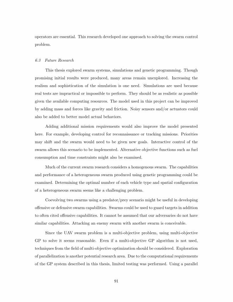
operators are essential. This research developed one approach to solving the swarm control
problem.
6.3 Future Research
This thesis explored swarm systems, simulations and genetic programming. Though
promising initial results were produced, many areas remain unexplored. Increasing the
realism and sophistication of the simulation is one need. Simulations are used because
real tests are impractical or impossible to perform. They should be as realistic as possible
given the available computing resources. The model used in this project can be improved
by adding mass and forces like gravity and friction. Noisy sensors and/or actuators could
also be added to better model actual behaviors.
Adding additional mission requirements would also improve the model presented
here. For example, developing control for reconnaissance or tracking missions. Priorities
may shift and the swarm would need to be given new goals. Interactive control of the
swarm allows this scenario to be implemented. Alternative objective functions such as fuel
consumption and time constraints might also be examined.
Much of the current swarm research considers a homogenous swarm. The capabilities
and performance of a heterogeneous swarm produced using genetic programming could be
examined. Determining the optimal number of each vehicle type and spatial configuration
of a heterogeneous swarm seems like a challenging problem.
Coevolving two swarms using a predator/prey scenario might be useful in developing
offensive or defensive swarm capabilities. Swarms could be used to guard targets in addition
to often cited offensive capabilities. It cannot be assumed that our adversaries do not have
similar capabilities. Attacking an enemy swarm with another swarm is conceivable.
Since the UAV swarm problem is a multi-objective problem, using multi-objective
GP to solve it seems reasonable. Even if a multi-objective GP algorithm is not used,
techniques from the field of multi-objective optimization should be considered. Exploration
of parallelization is another potential research area. Due to the computational requirements
of the GP system described in this thesis, limited testing was performed. Using a parallel
91

platform would allow many more evaluations to be performed in a reasonable amount of
time. A parallel approach would also be useful for studying GP evolution with multiple
populations.
6.4 Summary
The research presented in this document has illustrated that genetic programming
is a viable approach to developing control systems for UAV swarms. A three-dimensional
environment and vehicle model were developed with an emphasis placed on realistic ca-
pabilities. A hand-coded controller was developed and compared with the performance of
the evolved control programs. The evolved program trees did not outperform the human-
designed controller, but were competitive.
A major benefit of this approach is that genetic programming automatically created
the control system, using only information about the system. For the simplistic config-
uration used in this project, the benefit is not great. When attempting to develop more
complex systems though, genetic programming may be able to locate novel approaches
that humans would not likely find.
92

Appendix A. Unmanned Aerial Vehicles
Unmanned Aerial Vehicles (UAVs) are not a new technology. They have been used in
various forms for over 150 years. The Austrian military was the first to use unmanned
air vehicles in battle. During the seige of Venice, in 1849, Austrian Field Marshall Joseph
Radetzky attempted to bombard the city with explosive projectiles dropped from balloons
[61]. It is estimated that 200 balloons were launched in the attack. A fuse was set to
burn through the bombs support just as the device drifted over the intended target. By
all available accounts, the attack was a tremendous failure [61]. The unpredictability of
the flight path of a balloon was a serious hinderance to effective employment.
In 1863, Charles Perley was awarded a patent for Improvement in discharging ex-
plosive shells from balloons. [56, 76] Perleys device was a balloon with a hinged bottom.
Explosives would be placed in the basket. A timing device was used to trigger the lighting
of the fuse and release of the explosives. It is uncertain whether Perleys invention was ever
used [76, 56], but it would have suffered the same limitations as its predecessor.
Though these historical examples provide the earliest examples of unmanned air
vehicles, they are not considered UAVs. According to DoD Joint Publication 1-02, DoD
Dictionary a UAV is: A powered, aerial vehicle that does not carry a human operator, uses
aerodynamic forces to provide vehicle lift, can fly autonomously or be piloted remotely,
can be expendable or recoverable, and can carry a lethal or non-lethal payload. Ballistic or
semi ballistic vehicles, cruise missiles, and artillery projectiles are not considered unmanned
aerial vehicles. [79]
Often considered the first UAV, the Curtiss-Sperry Aerial Torpedo is more like a
cruise missile [34, 99]. The Aerial Torpedo was a modified Curtiss N-9 seaplane developed
by Elmer Sperry. Control of the aircraft was handled by an autopilot system using a
preprogrammed sequence of instructions. On March 6, 1918, the first successful flight was
conducted off the coast of Copiague, Long Island, New York [34, 24]. Though recovered
and later reflown, the Aerial Torpedo does not completely fit the DoD concept of UAVs.
The key discriminants are (1) UAVs are equipped and employed for recovery at the end of
93

their flight, and cruise missiles are not, and (2) munitions carried by UAVs are not tailored
and integrated into their airframe whereas the cruise missiles warhead is. [79]
The first returnable and reusable UAV was the British Fairey Queen [56, 34]. This
new generation of UAVs, the first to be considered true UAVs, was controlled using radio
signals. The Fairey Queen was first flown in September, 1932 [34]. An American system
called the Radioplane RP-1 was demonstrated to the Army Air Corps in 1935 [75].
Unmanned aerial vehicles were used in the Korean War, Vietnam War, Gulf War,
Balkans, Afghanistan and most recently during the Iraq War [35]. Improvements in tech-
nology have allowed UAVs to expand into areas beyond reconnaissance. The Predator is an
excellent example of this. Originally designed for reconnaissance, it was updated in 2001
to carry and launch the Hellfire missile. During the 1990s, DoD invested over $3 billion in
UAV development, procurement and operations. [79] By 2010, DoD projects spending of
$3 billion per year on UAV systems [79].
It was not until very recently that UAVs have gained much notariety. Other nations
are very interested in developing and fielding UAV systems. Thirty-two nations are devel-
oping or manufacturing over 250 models of UAVs [79] Additionally, 41 countries currently
operate 80 different types of UAVs, mostly for reconnaissance [79].
94

Appendix B. Genetic Programming Algorithm
1. t := 0;
2. initialize P (0) := π1(0), . . . , πµ(0) ∈ Π
3. evaluate P (0) : π1(0), . . . , πµ(0)
4. while (i(P (t)) 6= true) do
(a) reproduce : π′k(t) := rpr(P (t)) ∀k ∈ 1, . . . , µ;
(b) recombine : π′′k (t) := rpc(P (t)) ∀k ∈ 1, . . . , µ;
(c) mutate : π′′′k (t) := mpm(P (t)) ∀k ∈ 1, . . . , µ
(d) evaluate : P′′′
(t) := π′′′1 (t), ..., π
′′′µ (t) : Φ(π
′′′1 (t), . . . ,Φ(π
′′′µ (t))
(e) select : P (t + 1) := s(P′′′
(t))
where ps(π′′′k (t)) =
E[Fk(P ′′′ (t))]
µ=
ρ′
Fk(P ′′′ (t))
µ · ρFk(P ′′′ (t))
=
(RFkP ′′′ (t))
)q−(ρ
′
Fk(P ′′′ (t))
)q
µ · ρFk(P ′′′ (t))
(f)
RFi =i=j∑j=1
ρFj(P ) and ρFi(P′′′ (t)) =
1µ·
µ∑j=1
1 if Φ(πj) = Φ(πi)
0 otherwise
(g) t := t + 1;
5. od
The above is an outline of the basic Genetic Programming algorithm using the stan-
dard operators of reproduction, recombination and mutation. The population consists of
a set of valid computer programs composed of the functional and terminal symbols de-
fined by the user (2). The population is randomly initialized. Each individual is evaluated
and assigned a fitness value based on performance (3). Individuals from the population
are reproduced, recombined and mutated based on the probabilities associated with those
operators (4a - 4c). Tournament selection is used with tournament size q (4e) [8].
95

Furthermore, the generic GP algorithm is defined by the tuple:
GP = (Π,Φ,Ω,Ψ, s, i, µ, λ) ↔
(1)
π ∈ Π =β⋃
i=α
valid-programs(F , T , i)
where valid-programs(F , T , i) is the set of all valid computer programs using only
the function set F , terminal set T and having a maximum tree depth of i. The
minimum and maximum tree depths are given by α and β respectively.
Valid programs may be represented in list form using the following grammar: S → E
E → ( E ) | ( F ) | TERMINAL
F → F E E | FUNCTION
TERMINAL ∈ T
FUNCTION ∈ F
(2) ∀π ∈ Π : Φ(π) = f(π) where f(π) is the result returned by executing program π.
(3) Ω = mpm : πµ → πµ, cpc : πµ → πµ, rpr : πµ → πµ where the mutation
(m), crossover (c) and reproduction (r) operators are all the standard operators
defined by Koza in [53].
(4) Ψ = s(mpm(cpc(P ) ∪ rpr(P ))) is the generation transformation function.
(5) s : πµ → πmu, is the tournament selection operator. First q individuals are
randomly sampled from the population. The the individual with the highest fitness
of the group is selected.
(6) i(P (t)) =
true, if ∃k : Φ(πk) = 0
false, otherwise, stop only if the optimal fitness is reached.
Usually GP runs are stopped by a generation limit, even if an optimal solution is
found. It may be that a less complex, optimal individual can be evolved.
(7) λ = µ.
96

Appendix C. The Code Growth Problem in Genetic Programming
One of the major concerns with using a variable length solution representation is the size
of the resulting individuals [14, 43, 58, 67, 95]. The time required to evaluate an individual
depends on the size of the parse tree. Larger trees contain more functions and consequently
take longer to evaluate. This increase in solution size may be an acceptable trade-off if
increasingly fit individuals are evolved. Unfortunately, the growth of individual solutions
does not appear to be driven by increases in fitness [67, 58]. This problem has been
referred to in the literature by different names including: ‘bloat’ [14, 58, 67], ‘size problem’
[14, 43, 53] and ‘code growth’ [93, 95].
In order to find solutions to the code growth problem one must understand the
nature of the problem. There have been several attempts to explain why larger and larger
programs are evolved even though fitness remains stagnant [93, 58, 78, 95]. The simplest
and most common explanation is that introns are used to shield individuals against the
harmful effects of crossover. Introns are non-coding sections of a genome [19]. These
sections of the genotype may change without affecting the phenotype [19, 93]. An example
intron is the numerical expression E in: (* E 0). No matter what E evaluates to, the entire
expression is equal to 0. Introns are a cause of code bloat in GP, but not the only cause
[93, 58, 95].
Another theory of code growth was proposed by Langdon and Poli [59] and is based
on the distribution of solutions [95]. There may be many program trees (genotypes) that
produce the same fitness value (phenotype). These programs differ syntactically, but are
the same semantically [95]. Langdon and Poli argue that for the same fitness value, larger
solutions have a greater chance of being located since they greatly outnumber the smaller
solutions. In order for this hypothesis to be true, the larger programs must be easier to
find. It is not immediately obvious whether this is true or not [95].
A third explanation for increasing solution sizes is the “removal bias” of crossover
[58, 95]. The crossover operator first selects a subtree S to replace in parent A. If S is
smaller than the average subtree of A, then it is more likely to contain only introns [95].
In this case the offspring will have the same fitness as its parent. Since no code used
97

in the evaluation is modified, there can be no change in fitness. The new subtree from
parent B will be the size of the average subtree of B. The result is that on average, in cases
where fitness values are not affected, smaller subtrees are replaced by larger subtrees [95].
Searching for other potential causes of code growth is an active area of research in GP.
In order for GP to scale up to larger problems, the code growth problem must be
handled effectively. Several approaches to eliminating code growth have been studied
[14, 93, 43, 58, 67, 92]. The technique most often used is to set a maximum size or depth
limit for all individuals [53]. Individuals generated during reproduction which exceed the
size limit are discarded.
A similar approach using a dynamic maximum depth produced good results on even-
3 parity and symbolic regression problems [92]. This approach uses a dynamic limit in
addition to a strict limit. Like standard static depth limiting, individuals larger than the
dynamic limit are immediately rejected. Individuals larger than the dynamic limit, but
smaller than the strict limit, are evaluated. If the individual has a greater fitness than the
current best individual of the run, it is accepted in the new generation. Otherwise, the
individual is rejected. When a larger individual is accepted the dynamic limit is updated
to match the new best individual [92]. A decrease in population diversity was noted. This
could limit the exploration of the search space [92].
The use of explicitly defined introns (EDIs) was introducted to GP by Nordin [78].
Explicitly defined introns have also been applied to GAs [78]. In GP, an EDI is a special
function that is never evaluated when executing evolved programs. Though EDIs have
no effect on program evaluation, they are used when determining crossover points. Ex-
plicitly defined introns provide protection against building block disruption by crossover.
Improvements in fitness and efficiency have been reported when using EDIs [78]. Harries
and Smith used EDIs to assist with measuring and analyzing intron behavior [93].
Another approach using the concept of introns was proposed by Blickle and Thiele
[14]. They used a specialized crossover operator. First, intron nodes are identified and
marked as redundant. Then crossover performed, but only for non-redundant nodes. This
98

forces all crossover operations to have an effect on fitness and prevents the population from
converging prematurely [14].
Code editing is another technique used to limit tree growth [67, 95]. Code editing
can be visualized as a form of tree pruning. An algorithm to locate and remove intron
nodes is executed on the program tree. This is typically performed at the end of a run
to simplify the solution [53, 95]. The benefits of removing introns during the evolutionary
process are typically offset by the costs of doing so. Furthermore, introns that are not
detected are able to exploit that weakness and proliferate throughout the population [95].
Psuedo-hillclimbing is a method where offspring are rejected if they do not have a
higher (or sometimes only different) fitness than their parents [67]. If an offpsring is rejected
from the next generation, the parent is copied instead. This technique was explored by
Harries and Smith [93] in combination with EDIs. They used the terms incremental fitness
selection (IFS) and changed fitness selection (CFS) [93]. Their results showed that IFS
could effectively control bloat and achieve a high level of fitness. Other studies have also
yielded encouraging results [67].
The inclusion of parsimony pressure is another technique that is often used to steer
the evolutionary process toward simpler solutions. There are several different ways of
adding parsimony pressure to the GP system. The simplest way is by adding an additional
term to the fitness function [14, 67, 95]. This technique is called parametric parsimony
pressure or linear parsimony pressure. A typical fitness function using this method is:
g(x) = af(x) − bs; where f(x) is the raw fitness, g(x) is the total fitness, s is the size of
the individual and a and b are some arbitrary constants[14, 67].
One difficulty with using the parametric approach is in tuning the parameters. This
is especially problematic when the fitness assessment is nonlinear and when the population
converges near a certain fitness level [67]. Similar problems motivated the use of tour-
nament selection over fitness proportionate selection [67]. Parametric parsimony pressure
can produce smaller individuals but often results in decreased fitness [95].
A similar technique uses a minimum description length (MDL) principle [43]. The
fitness function for this approach is calculated from the tree coding length and exception
99

coding length. Iba et al. use a decision tree representation for their GP examples. Results
showed that the MDL-based fitness function generated smaller, more fit solutions. The
MDL approach is not a general solution since it only works on problems of a specific
structure [43].
Another approach to achieving parsimony is pareto parsimony pressure. Instead
of minimizing a single fitness function, pareto parsimony pressure uses a multiobjective
approach [67]. Pareto optimization is used to optimize multiple objectives when their
relative importance is unknown. In this approach, raw fitness and individual size are two
different objectives. This technique has yielded mixed results [67].
A new technique proposed by Luke and Panait [67] is lexicographic parsimony pres-
sure. Under this approach, raw fitness is the primary means of selection. If two individuals
have the same fitness then the smaller individual is chosen. Lexicographic parsimony pres-
sure outperformed standard depth limiting on the artificial ant, 11-bit boolean multiplexer
and even 5-parity problems [67].
It appears that the effectiveness of crossover decreases as trees grow larger [58].
Limiting individual tree size by evolving solutions as multiple smaller trees is one way to
solve this problem [58]. This is similar to the concept behind ADFs. Another approach is
to use a different crossover operator.
Langdon proposes two alternative crossover operators: size fair crossover and ho-
mologous crossover [57]. Size fair crossover limits the depth of replacement subtrees to
1 + 2 × |subtree to be deleted|. Though this limit does not appear very strict, programs
produced without it were 2.5 times larger than those using it [57]. Selection of crossover
points is biased to select subtrees of equal depth. Homologous crossover is similar to size
fair crossover. Homologous crossover deterministically selects the subtree in the second
parent that is closest in position to the one selected in the first parent. Closeness is de-
fined by the depth at which paths from the root to the subtree diverge [57]. While these
new crossover operators were successful in controlling tree growth, they were not more
effective at finding solutions on the problems tested [57].
100

Managing code growth continues to be a challenge in GP. Langdon has shown
that for standard GP, increases in program size reach a quadratic limit, ranging from:
O(generations1.2−2.0) [58]. This yields a run time of O(generations2.2−3.0) [58]. There are
several different ways to control the growth of program size in GP. Currently, no general
solution has been adopted. This remains an open area of research.
101

Appendix D. Portion of Steve Program Generated by Converter Software
The output of the genetic programming system is a symbolic expression. In order to use
the Breve simulation software, this s-expression must be converted into a Steve program.
S-Expression:
(vMult
(vMult
(vAdd
(vSub getTargetPosition myClosestNeighbor)
(vSub getAvgVelocity myCurVelocity))
(vDiv
(vSub getAvgVelocity myCurVelocity)
getTargetPosition))
(vMult
(vMult
(vAdd
(vSub getTargetPosition myClosestNeighbor)
(vSub getAvgVelocity myCurVelocity))
(vDiv
(vSub getAvgVelocity myCurVelocity)
getTargetPosition))
(vMult
(vAdd
(vDiv
(vSub getTargetPosition myClosestNeighbor)
getTargetPosition)
(vDiv
getClosestObstacle
(vAdd
(vMult
102

(vDiv
(vSub getAvgVelocity myCurVelocity)
getTargetPosition)
unitVector)
getClosestObstacle)))
getClosestObstacle)))
The corresponding Steve program code is presented below. Temporary variables
tVar# are used to store the results of vector calculations. Expressions are evaluated using
an in-order tree traversal. This means that each expression is evaluated once it is complete.
That is, when both of its children have been evaluated or are terminal symbols.
tVar0 = (self vSub one (self getTargetPosition) two (self myClosestNeighbor)).
tVar1 = (self vSub one (self getAvgVelocity) two (self myCurVelocity)).
tVar0 = (self vAdd one tVar0 two tVar1).
tVar1 = (self vSub one (self getAvgVelocity) two (self myCurVelocity)).
tVar1 = (self vDiv one tVar1 two (self getTargetPosition)).
tVar0 = (self vMult one tVar0 two tVar1).
tVar1 = (self vSub one (self getTargetPosition) two (self myClosestNeighbor)).
tVar2 = (self vSub one (self getAvgVelocity) two (self myCurVelocity)).
tVar1 = (self vAdd one tVar1 two tVar2).
tVar2 = (self vSub one (self getAvgVelocity) two (self myCurVelocity)).
tVar2 = (self vDiv one tVar2 two (self getTargetPosition)).
tVar1 = (self vMult one tVar1 two tVar2).
tVar2 = (self vSub one (self getTargetPosition) two (self myClosestNeighbor)).
tVar2 = (self vDiv one tVar2 two (self getTargetPosition)).
tVar3 = (self vSub one (self getAvgVelocity) two (self myCurVelocity)).
tVar3 = (self vDiv one tVar3 two (self getTargetPosition)).
tVar3 = (self vMult one tVar3 two (self unitVector)).
tVar3 = (self vAdd one tVar3 two (self getClosestObstacle)).
tVar3 = (self vDiv one (self getClosestObstacle) two tVar3).
103

tVar2 = (self vAdd one tVar2 two tVar3).
tVar2 = (self vMult one tVar2 two (self getClosestObstacle)).
tVar1 = (self vMult one tVar1 two tVar2).
tVar0 = (self vMult one tVar0 two tVar1).
104

Appendix E. Evolved Controller Programs in Symbolic Expression Form
E.1 Test 5 Best of Run
Fitness = 39965.2524638
(vMult
(vAdd
(vSub getTargetPosition myClosestNeighbor)
(vSub unitVector myCurVelocity))
(vDiv
(vSub getAvgVelocity myCurVelocity)
getTargetPosition))
E.2 Test 6 Best of Run
Fitness = 68525.3455516
(vAdd
(vMult
(vMult
(vDiv myCurVelocity getClosestObstacle)
(vAdd unitVector myClosestNeighbor))
(vDiv
(vSub doubleVector unitVector)
(vDiv
(vAdd
(vAdd
(vMult doubleVector doubleVector)
(vSub getTargetPosition getTargetPosition))
(vMult
(vMult doubleVector doubleVector)
(vSub unitVector doubleVector)))
105

(vSub
(vSub
(vAdd getTargetPosition getClosestObstacle)
(vMult myCurVelocity myCurVelocity))
(vMult
(vDiv getTargetPosition doubleVector)
(vMult getTargetPosition myCurVelocity))))))
(vSub getTargetPosition myClosestNeighbor))
106

Appendix F. Complete Statistical Results of Controller Performance
Baseline HandCoded w/getAvgVelocity w/o getAvgVelocityMean 71789.22 94683.94 133506.16Median 72495.76 84373.90 132482.20Minimum 0.00 2700.92 26176.39Maximum 183977.99 230390.22 277001.23Variance 1909926962.19 2507999385.69 2849704502.45Std Deviation 43702.71 50079.93 53382.62Map2 HandCoded w/getAvgVelocity w/o getAvgVelocityMean 95991.49 113058.42 153140.49Median 89220.82 107949.12 137008.87Minimum 3994.45 10890.78 43760.84Maximum 270843.54 316744.86 372649.10Variance 2947535358.57 2535845505.39 4568588412.83Std Deviation 54291.21 50357.18 67591.33Map3 HandCoded w/getAvgVelocity w/o getAvgVelocityMean 188598.94 249259.16 330394.96Median 165086.33 253873.37 318888.26Minimum 20224.47 1860.57 37806.94Maximum 610615.02 570453.02 758219.78Variance 13602565806.15 15720026655.35 26935820903.16Std Deviation 116630.04 125379.53 164121.36
Table 13 Statistical results for fitness values comparing different maps (n=100)
107

Size 40 HandCoded w/getAvgVelocity w/o getAvgVelocityMean 293544.46 347020.59 445074.83Median 290865.92 340889.16 431982.87Minimum 73905.71 187204.66 225471.92Maximum 553911.26 636019.17 634271.92Variance 9153974020.07 5950508540.59 8875072612.11Std Deviation 95676.40 77139.54 94207.60Size 60 HandCoded w/getAvgVelocity w/o getAvgVelocityMean 652720.80 732181.92 847532.54Median 652565.83 723193.23 845843.70Minimum 352814.99 503515.32 556788.20Maximum 1021883.90 1108122.68 1169171.36Variance 18308570596.08 12182235200.22 13905908027.80Std Deviation 135309.17 110373.16 117923.31
Table 14 Statistical results for fitness values comparing different swarm sizes (n=100)
Baseline HandCoded w/getAvgVelocity w/o getAvgVelocityMean 59.79 53.93 50.88Median 58.00 54.00 50.00Minimum 43.00 36.00 36.00Maximum 80.00 76.00 66.00Variance 69.00 55.20 46.21Std Deviation 8.31 7.43 6.80Map2 HandCoded w/getAvgVelocity w/o getAvgVelocityMean 57.16 45.05 47.85Median 57.00 44.00 48.00Minimum 37.00 25.00 24.00Maximum 77.00 67.00 64.00Variance 63.79 48.78 63.22Std Deviation 7.99 6.98 7.95Map3 HandCoded w/getAvgVelocity w/o getAvgVelocityMean 85.78 78.17 75.21Median 86.00 76.00 75.50Minimum 53.00 53.00 47.00Maximum 110.00 116.00 104.00Variance 149.35 143.94 154.63Std Deviation 12.22 12.00 12.44
Table 15 Statistical results comparing number of targets reached for different maps(n=100)
108

Size 40 HandCoded w/getAvgVelocity w/o getAvgVelocityMean 92.95 87.66 81.38Median 92.50 88.00 82.00Minimum 64.00 60.00 64.00Maximum 129.00 106.00 104.00Variance 145.38 74.00 83.67Std Deviation 12.06 8.60 9.15Size 60 HandCoded w/getAvgVelocity w/o getAvgVelocityMean 112.81 110.76 105.32Median 112.50 111.00 105.00Minimum 78.00 76.00 80.00Maximum 149.00 132.00 131.00Variance 192.94 111.88 108.12Std Deviation 13.89 10.58 10.40
Table 16 Statistical results comparing number of targets reached for different maps(n=100)
Baseline HandCoded w/getAvgVelocity w/o getAvgVelocityMean 5.98 9.09 10.48Median 6.00 9.00 11.00Minimum 0.00 2.00 4.00Maximum 10.00 15.00 16.00Variance 5.70 6.08 5.08Std Deviation 2.39 2.47 2.25Map2 HandCoded w/getAvgVelocity w/o getAvgVelocityMean 6.33 9.04 10.67Median 6.00 9.00 10.00Minimum 0.00 4.00 6.00Maximum 12.00 14.00 16.00Variance 5.92 4.24 4.99Std Deviation 2.43 2.06 2.23Map3 HandCoded w/getAvgVelocity w/o getAvgVelocityMean 7.10 8.94 10.09Median 7.00 9.00 10.00Minimum 2.00 0.00 3.00Maximum 14.00 14.00 16.00Variance 6.09 6.36 6.35Std Deviation 2.47 2.52 2.52
Table 17 Statistical results comparing number of crashes for different maps (n=100)
109

Size 40 HandCoded w/getAvgVelocity w/o getAvgVelocityMean 18.70 25.10 26.84Median 19.50 25.00 27.00Minimum 10.00 17.00 19.00Maximum 26.00 35.00 35.00Variance 10.74 7.46 9.17Std Deviation 3.28 2.73 3.03Size 60 HandCoded w/getAvgVelocity w/o getAvgVelocityMean 34.11 43.20 44.91Median 34.00 43.00 45.00Minimum 26.00 34.00 37.00Maximum 44.00 51.00 54.00Variance 13.15 11.80 9.78Std Deviation 3.63 3.43 3.13
Table 18 Statistical results comparing number of crashes for different maps (n=100)
Baseline HandCoded w/getAvgVelocity w/o getAvgVelocityMean 54380.03 19571.42 10596.84Median 54463.50 19824.03 9878.45Minimum 50902.74 14418.70 7559.10Maximum 57777.78 22387.95 17498.71Variance 2369377.72 3207713.06 4074374.15Std Deviation 1539.28 1791.01 2018.51Map2 HandCoded w/getAvgVelocity w/o getAvgVelocityMean 92239.24 26450.30 16893.84Median 92620.84 26485.66 16372.40Minimum 88736.15 25033.84 13782.28Maximum 94463.54 27302.41 24256.55Variance 1385275.80 147592.53 4294243.79Std Deviation 1176.98 384.18 2072.26Map3 HandCoded w/getAvgVelocity w/o getAvgVelocityMean 84661.99 33884.91 20078.57Median 84744.55 34177.12 19751.22Minimum 80779.64 25686.83 14501.43Maximum 87706.34 42050.97 27231.25Variance 2175415.12 12915070.60 8691782.77Std Deviation 1474.93 3593.75 2948.18
Table 19 Statistical results for mean distance to current target (n=100)
110

Size 40 HandCoded w/getAvgVelocity w/o getAvgVelocityMean 59197.42 20271.75 10450.32Median 59077.85 20678.83 10055.43Minimum 53997.43 15910.18 7830.71Maximum 64285.82 22014.87 16752.30Variance 3759326.26 2087142.48 3338779.96Std Deviation 1938.90 1444.69 1827.23Size 60 HandCoded w/getAvgVelocity w/o getAvgVelocityMean 61833.22 20145.87 10385.68Median 61721.35 20569.77 10086.39Minimum 56110.14 16646.59 7934.07Maximum 68147.65 22141.27 15311.30Variance 4771127.70 2144414.07 2357173.91Std Deviation 2184.29 1464.38 1535.31
Table 20 Statistical results for mean distance to current target (n=100)
Baseline HandCoded w/getAvgVelocity w/o getAvgVelocityMean 10580.75 7201.50 1683.90Median 10515.68 6973.81 1495.62Minimum 7360.36 3738.57 594.88Maximum 13743.14 11742.82 5583.11Variance 1947646.30 2135936.19 757875.14Std Deviation 1395.58 1461.48 870.56Map2 HandCoded w/getAvgVelocity w/o getAvgVelocityMean 12177.14 8783.29 2215.48Median 12061.02 8907.72 2047.15Minimum 8971.26 6862.97 925.17Maximum 18127.01 10410.48 5609.83Variance 2964954.63 639596.13 1057406.58Std Deviation 1721.90 799.75 1028.30Map3 HandCoded w/getAvgVelocity w/o getAvgVelocityMean 16059.52 12409.64 5405.13Median 16240.60 12254.90 5270.76Minimum 11398.46 9042.30 1577.49Maximum 19793.94 16576.23 10280.73Variance 3106716.98 2672304.05 3556954.29Std Deviation 1762.59 1634.72 1885.99
Table 21 Statistical results for mean distance to swarm center (n=100)
111

Size 40 HandCoded w/getAvgVelocity w/o getAvgVelocityMean 15148.79 7837.10 1655.93Median 15222.17 7738.28 1495.61Minimum 11071.00 4546.75 744.00Maximum 19947.33 11525.59 5868.41Variance 2983273.10 1955651.56 646392.50Std Deviation 1727.22 1398.45 803.99Size 60 HandCoded w/getAvgVelocity w/o getAvgVelocityMean 17461.83 7744.76 1699.22Median 17268.97 7680.93 1564.22Minimum 12595.04 5189.79 824.77Maximum 22536.37 11009.55 4997.05Variance 3639878.95 1794212.49 444639.66Std Deviation 1907.85 1339.48 668.81
Table 22 Statistical results for mean distance to swarm center (n=100)
112

Bibliography
1. “AeroVironment’s “Wasp” Micro Air Vehicle Sets World Record.” News Release,August 2002.
2. “AeroVironment’s “Hornet” Micro Air Vehicle Completes First Fuel Cell PoweredFlight.” News Release, March 2003.
3. “Air Force Research Laboratory, Embedded Information Systems Engineering BranchMission Statement.”
4. “Air Force Research Laboratory, Information Technology Division Mission State-ment.”
5. Aler, R., Borrajo, D., and Isasi, P. “Using genetic programming to learn and improvecontrol knowledge,” Artificial Intelligence, 141 (1):29–56 (2002).
6. Andre, D. “The Automatic Programming of Agents that Learn Mental Models andCreate Simple Plans of Action.” IJCAI-95 Proceedings of the Fourteenth InternationalJoint Conference on Artificial Intelligence1 . 741–747. Montreal, Quebec, Canada:Morgan Kaufmann, 20-25 August 1995.
7. Anton, H. Calculus with Analytic Geometry (Fifth Edition). New York: John Wileyand Sons, Inc., 1995.
8. Back, T. Evolutionary Algorithms in Theory and Practice. New York: Oxford Uni-versity Press, 1996.
9. Back, T., Fogel, D. B., and Michalewicz, Z., editors. Evolutionary Computation1: Basic Algorithms and Operators. Bristol, United Kingdom: Institute of PhysicsPublishing Ltd., 2000.
10. Back, T., Fogel, D. B., and Michalewicz, Z., editors. Evolutionary Computation 2:Advanced Algorithms and Operators. Bristol, United Kingdom: Institute of PhysicsPublishing Ltd., 2000.
11. Baldassarre, G., Nolfi, S., and Parisi, D. “Evolving Mobile Robots Able to DisplayCollective Behaviors,” Artificial Life, 9 (3):255–268 (2003).
12. Bellingham, J., Tillerson, M., Richards, A., and How, J. P. “Multi-Task Allocationand Path Planning for Cooperating UAVs.” Cooperative Control: Models, Applica-tions and Algorithms edited by S. Butenko, et al., chapter 2, Kluwer, 2002.
13. Bellingham, J. S., Tillerson, M., Alighanbari, M., and How, J. P. “Cooperative PathPlanning for Multiple UAVs in Dynamic and Uncertain Environments.” Proceedingsof IEEE CDC . Dec 2002.
14. Blickle, T. and Thiele, L. “Genetic Programming and Redundancy.” Genetic Al-gorithms within the Framework of Evolutionary Computation (Workshop at KI-94,Saarbrucken), edited by J. Hopf. 33–38. Im Stadtwald, Building 44, D-66123Saarbrucken, Germany: Max-Planck-Institut fur Informatik (MPI-I-94-241), 1994.
113

15. Bonabeau, E., Dorigo, M., and Theraulaz, G. Swarm Intelligence: From Natural toArtificial Systems (Santa Fe Institute Studies on the Sciences of Complexity). Oxford,UK: Oxford University Press, 1999.
16. Brooks, R. A. “A Robust Layered Control System for a Mobile Robot,” IEEE Journalof Robotics and Automation, 2 (1) (1986).
17. Bugajska, M. D., Schultz, A. C., Trafton, J. G., Gittens, S., and Mintz, F. “Build-ing Adaptive Computer Generated Forces: The Effect of Increasing Task Reactivityon Human and Machine Control Abilities.” Genetic and Evolutionary ComputationConference Late Breaking Papers. 2001.
18. Bugajska, M. D. and Schultz, A. C. “Co-evolution of Form and Function in theDesign of Autonomous Agents: Micro Air Vehicle Project.” Workshop on Evolutionof Sensors GECCO 2000 . 240–244. Aug 2000.
19. Campbell, N. A., Mitchell, L. G., and Reece, J. B. Biology: Concepts and connections.Redwood City, California: Benjamin/Cummings Publishing Co., 1994.
20. Cao, Y. U., Fukunaga, A. S., Kahng, A. B., and Meng, F. “Cooperative Mo-bile Robotics: Antecedents and Directions.” International Conference on IntelligentRobots and Systems1 . August 1995.
21. Cazangi, R. R., von Zuben, F. J., and Figueiredo, M. “A Classifier System in RealApplications for Robot Navigation.” Conference on Evolutionary Computation. 2003.
22. Center, N. G. R., “Beginner’s Guide to Aerodynamics.” URL.
23. Chongstitvatana, P. “Improving Robustness of Robot Programs Generated by Ge-netic Programming for Dynamic Environments.” IEEE Asia Pacific Conference onCircuits and Systems (APCCAS). 523–526. 1998.
24. Clark, R. M. Uninhabited Combat Aerial Vehicles: Airpower by the People, for thePeople, but not with the People. CADRE Paper 8, Air University, 8 2000.
25. Corner, J. “Selecting a Simulator for Modeling UAV Swarms.” Air Force Institute ofTechnology, Department of Computer Engineering, 2003.
26. Coulouris, G., Dollimore, J., and Kindberg, T. Distributed Systems: Concepts andDesign (Third Edition). Harlow, England: Addison-Wesley, 1988.
27. Cramer, N. L. “A Representation for the Adaptive Generation of Simple SequentialPrograms.” Proceedings of an International Conference on Genetic Algorithms andtheir Applications, edited by John J. Grefenstette. 183–187. 1985.
28. Crombie, D. The Examination and Exploration of Algorithms and Complex Behaviourto Realistically Control Multiple Mobile Robots. MS thesis, The Austrailian NationalUniversity, 1997.
29. Daley, R., Schultz, A. C., and Grefenstette, J. J. “Co-evolution of Robot Behav-iors.” Proceedings of the SPIE International Symposium on Intelligent Systems andAdvanced Manufacturing . 19–22. Sept 1999.
114

30. Dudek, G., Jenkin, M. R. M., Milios, E., and Wilkes, D. “A Taxonomy for Multi-Agent Robotics,” Autonomous Robots, 3 :375–397 (1996).
31. Feddema, J. T., Lewis, C., and Schoenwald, D. A. “Decentralized Control of Coop-erative Robotic Vehicles: Theory and Application,” IEEE Transactions on Roboticsand Automation, 18 (5):852–864 (2002).
32. Fogel, L. J., Owens, A. J., and Walsh, M. J. Artificial Intelligence through SimulatedEvolution. New York: Wiley, 1966.
33. Foley, J. D., van Dam, A., Veiner, S. K., and Hughes, J. F. Computer Graphics:Principles and practice, Second Edition in C . Reading, Massachusetts: Addison-Wesley, 1990.
34. Forum, U., “UAV Forum: Frequently Asked Questions,” 2003.
35. Garamone, J., “From the U.S. Civil War to Afghanistan: A Short History of UAVs,”4 2002.
36. Gaudiano, P., Shargel, B., Bonabeau, E., and Clough, B. T. “Swarm Intelligence: aNew C2 Paradigm with an Application to Control of Swarms of UAVs.” 8th Interna-tional Command and Control Research and Technology Symposium. 2003.
37. Grasmeyer, J. M. and Keennon, M. T. “Development of the Black Widow Micro AirVehicle.” Proceedings of the 39th AIAA Aerospace Sciences Meeting . January 2001.Paper No. 2001-0127.
38. Harvey, I., Husbands, P., and Cliff, D. Issues in Evolutionary Robotics. TechnicalReport Cognitive Science Research Paper CSRP219, Brighton BN1 9QH, England,UK: The University of Sussex, School of Cognitive and Computing Sciences, 1992.
39. Haynes, T., Sen, S., Schoenefeld, D., and Wainwright, R. Evolving Multiagent Coordi-nation Strategies with Genetic Programming . Technical Report UTULSA-MCS-95-04,The University of Tulsa, May 31, 1995.
40. Haynes, T. D. and Wainwright, R. L. “A Simulation of Adaptive Agents in Hos-tile Environment.” Proceedings of the 1995 ACM Symposium on Applied Computing ,edited by K. M. George, et al. 318–323. Nashville, USA: ACM Press, 1995.
41. Holland, J. H. Adaptation in Natural and Artificial Systems: An introductory analy-sis with applications to biology, control, and artificial intelligence. Cambridge, Mas-sachusetts: MIT Press, 1975.
42. Holub, A. I. Compiler Design in C . Englewood Cliffs, New Jersey: Prentice-Hall,Inc., 1990.
43. Iba, H., de Garis, H., and Sato, T. “Genetic Programming Using a Minimum De-scription Length Principle.” Advances in Genetic Programming edited by Kenneth E.Kinnear, Jr., chapter 12, 265–284, MIT Press, 1994.
44. Ito, T., Iba, H., and Kimura, M. “Robustness of Robot Programs Generated byGenetic Programming.” Genetic Programming 1996: Proceedings of the First Annual
115

Conference, edited by John R. Koza, et al. Stanford University, CA, USA: MIT Press,28–31 July 1996. 321–326.
45. Jamshidi, M., dos Santos Coelho, L., Krohling, R. A., and Fleming, P. J. RobustControl Systems with Genetic Algorithms. Boca Raton, Florida, USA: CRC Press,2003.
46. Jun, M. and D’Andrea, R. “Path Planning for Unmanned Aerial Vehicles in Uncer-tain and Adversarial Environments.” Cooperative Control: Models, Applications andAlgorithms edited by S. Butenko, et al., chapter 6, Kluwer, 2002.
47. Kadrovach, A. B. A Communications Modeling System for Swarm-based Sensors.PhD dissertation, Air Force Institute of Technology, 2003.
48. Kahn, J. M., Howard, R., and Pister, K. S. J. “Emerging Challenges: Mobile Network-ing for “Smart Dust”,” IEEE Journal of Communications and Networks, 2 (3):188–196 (September 2000).
49. Klavins, E. “Automatically Synthesized Controllers for Distributed Assembly: PartialCorrectness.” Cooperative Control: Models, Applications and Algorithms edited byS. Butenko, et al., chapter 7, 111–127, Kluwer, 2002.
50. Klein, J. “BREVE: a 3D Environment for the Simulation of Decentralized Systemsand Artificial Life.” Proceedings of the Eighth International Conference on ArtificialLife. 329–334. 12 2002.
51. Klein, J., “BREVE: 3D Simulation and Visualization Software,” 2004.
52. Koerner, B. I. “What is Smart Dust, Anyway?,” Wired (June 2003).
53. Koza, J. R. Genetic Programming: On the Programming of Computers by Means ofNatural Selection. Cambridge, Massachusetts: The MIT Press, 1992.
54. Koza, J. R. Genetic Programming III: Darwinian Invention and Problem Solving .San Francisco: Morgan Kaufmann, 1999.
55. Koza, J. R. and Rice, J. P. “Automatic programming of robots using genetic program-ming.” Proceedings of Tenth National Conference on Artificial Intelligence. 194–201.AAAI Press/MIT Press, 1992.
56. Krock, L., “Spies that Fly: A Timeline of UAVs,” 11 2002.
57. Langdon, W. B. “Size Fair and Homologous Tree Genetic Programming Crossovers.”Proceedings of the Genetic and Evolutionary Computation Conference2 , edited byWolfgang Banzhaf, et al. 1092–1097. Orlando, Florida, USA: Morgan Kaufmann,13-17 July 1999.
58. Langdon, W. B. “Quadratic Bloat in Genetic Programming.” Proceedings of theGenetic and Evolutionary Computation Conference (GECCO-2000), edited by DarrellWhitley, et al. 451–458. Las Vegas, Nevada, USA: Morgan Kaufmann, 10-12 July2000.
116

59. Langdon, W. B. and Poli, R. Fitness Causes Bloat . Technical Report CSRP-97-09,Birmingham, B15 2TT, UK: University of Birmingham, School of Computer Science,24 February 1997.
60. Langdon, W. B. and Poli, R. Foundations of Genetic Programming . Berlin: Springer-Verlag, 2002.
61. Lavelle, B. C. “Zeppelinitis.” Air Command and Staff College, 3 1997.
62. Lazarus, C. and Hu, H. “Using Genetic Programming to Evolve Robot Behaviours.”Proceedings of the 3rd British Conference on Autonomous Mobile Robotics and Au-tonomous Systems. 2001.
63. Levine, J. R., Mason, T., and Brown, D. Lex and Yacc (Second Edition). Sebastopol,California: O’Reilly and Associates, Inc., 1990.
64. Lotspeich, J. T. Distributed Control of a Swarm of Autonomous Unmanned AerialVehicles. MS thesis, Air Force Institute of Technology, 2003.
65. Lua, C. A., Altenburg, K., and Nygard, K. E. “Synchronized Multi-Point Attack byAutonomous Reactive Vehicles with Simple Local Communication.” Proceedings ofthe IEEE Swarm Intelligence Symposium. 2003.
66. Luke, S., Balan, G. C., and Panait, L. “Population Implosion in Genetic Program-ming..” Genetic and Evolutionary Computation – GECCO-20032724 . LNCS, editedby E. Cantu-Paz, et al. 1729–1739. Chicago: Springer-Verlag, 12-16 July 2003.
67. Luke, S. and Panait, L. “Lexicographic Parsimony Pressure.” GECCO 2002: Pro-ceedings of the Genetic and Evolutionary Computation Conference, edited by W. B.Langdon, et al. 829–836. New York: Morgan Kaufmann Publishers, 9-13 July 2002.
68. Luke, S., Panait, L., Skolicki, Z., Bassett, J., Hubley, R., and Chircop, A., “ECJ: AJava-based Evolutionary Computation and Genetic Programming Research System,”2002.
69. Luke, S. and Spector, L. “Evolving Teamwork and Coordination with Genetic Pro-gramming.” Genetic Programming 1996: Proceedings of the First Annual Conference,edited by John R. Koza, et al. 150–156. Stanford University, CA, USA: MIT Press,28–31 July 1996.
70. Luke, S. and Spector, L. “A Revised Comparison of Crossover and Mutation inGenetic Programming.” Genetic Programming 1998: Proceedings of the Third An-nual Conference, edited by John R. Koza, et al. 208–213. University of Wisconsin,Madison, Wisconsin, USA: Morgan Kaufmann, 22-25 July 1998.
71. Matsumoto, M., “Mersenne Twister: A Random Number Generator,” 2004.
72. Milton, J. and Arnold, J. C. Introduction to Probability and Statistics: Principlesand Applications for Engineering and the Computing Sciences (Third Edition). NewYork: McGraw-Hill Primis Custom Publishing, 2002.
73. Montana, D. J. Strongly Typed Genetic Programming . BBN Technical Report #7866,10 Moulton Street, Cambridge, MA 02138, USA: Bolt Beranek and Newman, Inc., 7May 1993.
117

74. Moore, F. W. and Garcia, O. N. “A Genetic Programming Approach to StrategyOptimization in the Extended Two-Dimensional Pursuer/Evader Problem.” GeneticProgramming 1997: Proceedings of the Second Annual Conference, edited by John R.Koza, et al. 249–254. Stanford University, CA, USA: Morgan Kaufmann, 13-16 1997.
75. Naughton, R., “Remote Piloted Aerial Vehicles : An Anthology,” 2 2003.
76. Niepert, R., “Hot Air Balloons in the Civil War,” 2003.
77. Nordin, P. and Banzhaf, W. “Real Time Control of a Khepera Robot Using GeneticProgramming,” Cybernetics and Control , 26 (3) (1997).
78. Nordin, P., Francone, F., and Banzhaf, W. “Explicitly Defined Introns and De-structive Crossover in Genetic Programming.” Proceedings of the Workshop on Ge-netic Programming: From Theory to Real-World Applications, edited by Justinian P.Rosca. 6–22. 9 July 1995.
79. of the Secretary of Defense, O. Unmanned Aerial Vehicles Roadmap: 2002 – 2027 .Technical Report, United States Department of Defense, 12 2002.
80. O’Reilly, U.-M. and Oppacher, F. Hybridized Crossover-Based Search Techniques forProgram Discovery . Technical Report 95-02-007, 1399 Hyde Park Road Santa Fe,New Mexico 87501-8943 USA: Santa Fe Institute, 1995.
81. Perkis, T. “Stack-Based Genetic Programming.” Proceedings of the 1994 IEEE WorldCongress on Computational Intelligence1 . 148–153. Orlando, Florida, USA: IEEEPress, 27-29 June 1994.
82. Pister, K. S. J., “Smart Dust HomePage.”
83. Poli, R. “Evolution of Graph-like Programs with Parallel Distributed Genetic Pro-gramming.” Genetic Algorithms: Proceedings of the Seventh International Confer-ence, edited by Thomas Back. 346–353. Michigan State University, East Lansing,MI, USA: Morgan Kaufmann, 19-23 July 1997.
84. Poli, R. and Langdon, W. B. “On the Search Properties of Different CrossoverOperators in Genetic Programming.” Genetic Programming 1998: Proceedings of theThird Annual Conference, edited by John R. Koza, et al. 293–301. University ofWisconsin, Madison, Wisconsin, USA: Morgan Kaufmann, 22-25 July 1998.
85. Punch, B. and Goodman, E., “The lil-gp Genetic Programming System,” 9 1998.
86. Reynolds, C. W. “Flocks, Herds, and Schools: A Distributed Behavioral Model,”Computer Graphics, 21 (4):25–34 (1987).
87. Reynolds, C. W. “An Evolved, Vision-Based Behavioral Model of CoordinatedGroup Motion.” From Animals to Animats (Proceedings of Simulation of AdaptiveBehaviour), edited by Meyer and Wilson. MIT Press, 1992.
88. Reynolds, C. W. “Evolution of Corridor Following Behavior in a Noisy World.”Simulation of Adaptive Behaviour (SAB-94). 1994.
118

89. Reynolds, C. W. “An Evolved, Vision-Based Behavioral Model of Obstacle AvoidanceBehaviour.” Artificial Life III XVII . SFI Studies in the Sciences of Complexity, editedby Christopher G. Langton, 327–346, Santa Fe Institute, New Mexico, USA: Addison-Wesley, 15-19 June 1992 1994.
90. Samuel, A. L. “Some Studies in Machine Learning Using the Game of Checkers,”IBM Journal of Research and Development , 3 (3):210–229 (July 1959).
91. Serway, R. A. Physics for Scientists and Engineers (Fourth Edition), 1 . Philadelphia,Pennsylvania: Saunders College Publishing, 1982.
92. Silva, S. and Almeida, J. “Dynamic Maximum Tree Depth.” Genetic and EvolutionaryComputation – GECCO-20032724 . LNCS, edited by E. Cantu-Paz, et al. 1776–1787.Chicago: Springer-Verlag, 12-16 July 2003.
93. Smith, P. W. H. and Harries, K. “Code Growth, Explicitly Defined Introns, andAlternative Selection Schemes,” Evolutionary Computation, 6 (4):339–360 (Winter1998).
94. Sommerville, I. Software Engineering (Fifth Edition). Harlow, England: Addison-Wesley, 1996.
95. Soule, T. Code Growth in Genetic Programming . PhD dissertation, University ofIdaho, Moscow, Idaho, USA, 15 May 1998.
96. Spector, L. “Simultaneous Evolution of Programs and their Control Structures.”Advances in Genetic Programming 2 edited by Peter J. Angeline and K. E. Kinnear,Jr., chapter 7, 137–154, Cambridge, MA, USA: MIT Press, 1996.
97. Spector, L., Klein, J., Perry, C., and Feinstein, M. “Emergence of Collective Behaviorin Evolving Populations of Flying Agents.” Proceedings of the Genetic and Evolution-ary Computation Conference (GECCO), edited by E. Cantu-Paz, et al. 61–73. Berlin:Springer-Verlag, 2003.
98. Spector, L. and Robinson, A. “Genetic Programming and Autoconstructive Evolu-tion with the Push Programming Language,” Genetic Programming and EvolvableMachines, 3 (1):7–40 (March 2002).
99. Swanson, B., “Navy’s UAV Program Celebrates an Unmanned, Unremarked 79thBirthday: From Jenny to the Pegasus,” 10 2003.
100. Teller, A. and Veloso, M. “PADO: A New Learning Architecture for Object Recog-nition.” Symbolic Visual Learning edited by Katsushi Ikeuchi and Manuela Veloso,81–116, Oxford University Press, 1996.
101. Trahan, M. W., Wagner, J. S., Stantz, K. M., Gray, P. C., and Robinett, R. “Swarmsof UAVs and Fighter Aircraft.” Proceedings of the 2nd International Conference onNonlinear Problems in Aviation and Aerospace. 745–752. 1998.
102. Trianni, V., Grob, R., Labella, T. H., Sahin, E., and Dorigo, M. “Evolving Aggrega-tion Behaviors in a Swarm of Robots.” Advances in Artificial Life, 7th European
119

Conference, ECAL 2003, Dortmund, Germany, September 14-17, 2003, Proceed-ings2801 . Lecture Notes in Computer Science, edited by Wolfgang Banzhaf, et al.Springer-Varlag, 2003.
103. Tunstel, E. and Lippincott, T. “Genetic Programming of Fuzzy Coordination Behav-iors for Mobile Robots.” International Symposium on Soft Computing for Industry,2nd World Automation Congress. 647–652. 1996.
104. Vargas, P. A., de Castro, L. N., Michelan, R., and von Zuben, F. J. “Implementationof an Immuno-Genetic Network on a Real Khepera II Robot.” Proceedings of theIEEE Congress on Evolutionary Computation. Dec 2003.
105. Wu, A. S., Schultz, A. C., and Agah, A. “Evolving Control for Distributed Micro AirVehicles.” IEEE Computational Intelligence in Robotics and Automation EngineersConference. 1999.
106. Zhang, Y., Martinoli, A., and Antonsson, E. K. “Evolutionary Design of a CollectiveSensory System.” Proceedings of the 2003 AAAI Spring Symposium on ComputationalSynthesis, edited by H. Lipson, et al. 283–290. AAAI Press, 2003.
120

5(3257'2&80(17$7,213$*( )RUP$SSURYHG
20%1R
5(3257'$7(''00<<<< 5(32577<3(
7,7/($1'68%7,7/(
D&2175$&7180%(5
$87+256
3(5)250,1*25*$1,=$7,211$0(6$1'$''5(66(6
6321625,1*021,725,1*$*(1&<1$0(6$1'$''5(66(6
3(5)250,1*25*$1,=$7,21
5(3257180%(5
6321625021,7256$&521<06
6833/(0(17$5<127(6
',675,%87,21$9$,/$%,/,7<67$7(0(17
$%675$&7
68%-(&77(506
180%(5
2)
3$*(6
D1$0(2)5(63216,%/(3(5621
D5(3257
E$%675$&7 F7+,63$*(
/,0,7$7,212)
$%675$&7
6WDQGDUG)RUP5HY
3UHVFULEHGE\$16,6WG=
7KHSXEOLFUHSRUWLQJEXUGHQIRUWKLVFROOHFWLRQRI LQIRUPDWLRQLVHVWLPDWHGWRDYHUDJHKRXUSHUUHVSRQVH LQFOXGLQJWKHWLPHIRUUHYLHZLQJLQVWUXFWLRQVVHDUFKLQJH[LVWLQJGDWDVRXUFHV
JDWKHULQJDQGPDLQWDLQLQJWKHGDWDQHHGHGDQGFRPSOHWLQJDQGUHYLHZLQJWKHFROOHFWLRQRILQIRUPDWLRQ6HQGFRPPHQWVUHJDUGLQJWKLVEXUGHQHVWLPDWHRUDQ\RWKHUDVSHFWRIWKLVFROOHFWLRQ
RI LQIRUPDWLRQ LQFOXGLQJ VXJJHVWLRQV IRU UHGXFLQJ WKH EXUGHQ WR 'HSDUWPHQW RI 'HIHQVH :DVKLQJWRQ +HDGTXDUWHUV 6HUYLFHV 'LUHFWRUDWH IRU ,QIRUPDWLRQ 2SHUDWLRQV DQG 5HSRUWV
-HIIHUVRQ'DYLV+LJKZD\6XLWH$UOLQJWRQ9$5HVSRQGHQWVVKRXOGEHDZDUHWKDWQRWZLWKVWDQGLQJDQ\RWKHUSURYLVLRQRIODZQRSHUVRQVKDOOEH
VXEMHFWWRDQ\SHQDOW\IRUIDLOLQJWRFRPSO\ZLWKDFROOHFWLRQRILQIRUPDWLRQLILWGRHVQRWGLVSOD\DFXUUHQWO\YDOLG20%FRQWUROQXPEHU
3/($6('21275(7851<285)250727+($%29($''5(66
'$7(6&29(5(')URP7R
E*5$17180%(5
F352*5$0(/(0(17180%(5
G352-(&7180%(5
H7$6.180%(5
I:25.81,7180%(5
6321625021,72565(3257
180%(56
6(&85,7<&/$66,),&$7,212)
E7(/(3+21(180%(5,QFOXGHDUHDFRGH