Embed Size (px)
Citation preview
1
Evolution of Monetary Policy in the US: The Role of Asset Prices
Beatrice D. Simo-Kengne Department of Economics
University of Pretoria Pretoria, 0002
SOUTH AFRICA [email protected]
Stephen M. Miller*
Department of Economics University of Nevada, Las Vegas Las Vegas, Nevada, 89154-6005
and
Rangan Gupta
Department of Economics University of Pretoria
Pretoria, 0002 SOUTH AFRICA
Abstract. This paper investigates whether changes in monetary transmission mechanism respond to variations in asset prices. We distinguish between bull and bear markets and employ a TVP-VAR approach with stochastic volatility to assess the evolution of the monetary policy in relation to housing and stock prices. We measure the relative importance of housing and stock prices in the conduct of monetary policy and their possible feedback effects over both time and horizon and across regimes. Empirical results from annual data on the US spanning the period from 1890 to 2012 indicate that monetary policy responds more strongly to asset prices during bull regimes. While the bigger monetary effect of stock price shocks occurs prior to the 1970s, monetary policy appears to respond more strongly to housing price than stock price shocks after the 1970s. Similarly, contractionary monetary policy exerts a larger effect on both asset categories during bull markets. Particularly, larger negative responses of house prices to monetary policy shocks occur after the 1980s, corresponding to the bull regime in the housing market. Conversely, the stock-price effect of monetary policy shocks dominates before the 1980s, where stock-market booms achieved more importance. Keywords: Monetary policy, house prices, stock prices, TVP-VAR JEL classification: C32, E52, G10 * Corresponding author.
2
1. Introduction
The early 1980s saw the beginning of the Great Moderation, when many macroeconomic
variables exhibited decreased volatility. Debate followed about the causes of this moderation.
Did it reflect good policy or good luck? The good-luck proponents argued that policy makers
now understood how to moderate the business cycle. The Great Moderation also saw a general
fall in inflation rates around the world. A leading explanation of the declining inflation rates
relied on inflation targeting, which many central banks adopted over this time frame. Of course,
the financial crisis and Great Recession shattered that optimistic view of the policy making
process and the ability of policy makers to moderate business cycle movements.1
During the Great Moderation, however, asset prices became more volatile, leading
eventually to the financial crisis and Great Recession. Borio et al., (1994) and Detken and Smets
(2004) report the emergence of the boom-bust cycles in equity and housing prices across many
developed countries during the 1980s. Further, Bernanke and Gertler (2004) argue that the
increased asset price volatility caught the attention of researchers and policy makers, especially
since central bankers apparently now knew how to control inflation.
This study adopts a Time Varying Parameter Vector Autoregressive (TVP-VAR)
approach beginning with a Markov Switching Autoregressive (MS-AR) model to assess the
evolution of the monetary policy in relation to asset prices over the annual period of 1890 to
2012. Unlike previous studies, our approach measures the relationship between the two variables
not only over different time and horizons and more importantly across different regimes. Thus,
1 For example, Kim and Nelson (1999), McConnell and Perez-Quiros (2000), Blanchard and Simon (2001), and Ahmed et al. (2004), among others, document a structural change in the volatility of U.S. GDP growth, finding a rather dramatic reduction in GDP volatility. Stock and Watson (2003), Bhar and Hamori (2003), Mills and Wang (2003), and Summers (2005) show a structural break in the volatility decline of the output growth rate for Japan and other G7 countries, although the break occurs at different times.
3
the approach can account for historical episodes of structural changes such as the Great
Depression (1930s), the Great Inflation (1970s), the Great Moderation (1980s through mid-
2000s), and the Great Recession (late-2000s) with time varying effects on VAR parameters.
A growing literature emphasizes the role of asset price fluctuations in driving financial
and business cycle dynamics (e.g., Bernanke and Gertler). First, asset price variation potentially
affects the real economy as a consequence of a direct effect on household wealth on consumption
demand (e.g., Zhou and Carroll, 2012; Case et al. 2013; Liu et al., 2013; Guerrieri and
Iacoviello, 2013; Mian et al., 2013). Second, the balance sheet channel argues that credit markets
include significant frictions, whereby those borrowers with strong financial credentials stand a
better chance of obtaining a loan than borrowers with weak financial credentials. Additionally,
forward-looking, rational economic agents incorporate the fluctuation in asset prices in their
expectations (Gelain and Lansing, 2013), which, in turn, affects the propagation mechanism of
shocks.
The emergence of inflation in asset prices caused a reappraisal of what monetary policy
makers should or should not do when faced with rapid increases in asset prices. Bernanke and
Gertler (2001) argue that policy makers do not need to respond to rising asset prices that reflect
changing fundamentals in asset markets. Rather policy makers need to pay attention when asset
prices rise because of non-fundamental factors and when asset price changes cause important
effects in the macroeocnomy. The ability of policy makers to identify the difference between
fundamental and non-fundamental changes in asset prices proves most difficult. Thus, any policy
that requires the central bank to diffuse asset price inflation before it forms a bubble requires that
the central bank identify bubble situations before and during their formation, no easy task
4
An additional problem faces monetary policy makers when faced with rising asset prices.
Traditional monetary policy focuses on controlling inflation, typically measured by the consumer
price index. But, this measure of inflation excludes asset price inflation. How should policy
makers respond to a situation of low consumer price inflation coupled with rapid inflation in
equity and real estate prices?
Asset price shocks precipitate reactions from the policy makers and, hence, modify the
transmission mechanism of macroeconomic policies. Two related issues are of particular interest.
How can monetary policy makers use asset price shocks to improve its ability to pursue financial
and macroeconomic stability? Hoes does monetary policy affect asset prices? In fact, the recent
global financial crisis and the subsequent Great Recession in the US, prompted by the crash of
housing and stock markets, highlight the importance of these asset prices as instruments for the
monetary authorities. These events renewed the interest of researchers and policy makers in the
linkages between monetary policy and asset prices, particularly, housing and stock prices.
As noted above, developments in asset markets may respond to monetary policy while at
the same time, fluctuations in asset prices likely affect the conduct of the monetary policy. Bordo
and Wheelock (2004) discuss three different arguments for how asset price bubbles develop.
First, the traditional view argues that an asset price boom results from the growth in the money
supply. The excess liquidity causes asset prices to rise and, thus, transmits the monetary policy
strategy to the entire economy. Second, Bordo and Wheelock refer to the Austrian or Bank of
International Settlements (BIS) view, where rising asset prices can degenerate into a bubble
situation when the policy makers do not intervene to control the expansion of credit. That is, the
policy makers enter a situation where consumer price inflation remains benign while asset price
inflation enters a bubble. Third, researchers examine equilibrium rational expectations models
5
can generate asset price bubbles monetary authorities do not commit to a stead long-run inflation
rate.
Given the stability goal of modern economies, numerous studies assess the interplay
between asset prices and the US monetary policy with contradicting results. One reason for
disparate findings reflects the fact that monetary policy experienced dramatic evolution over the
past decades.2 On the one hand, Bernanke and Gertler (2001) indicate that no need exists for
monetary policy to react to asset price fluctuations, except to the extent that they help forecasting
inflation. Similarly, Filardo (2000) finds little evidence that the use of real estate and equity
prices can improve the conduct of the monetary policy. Further, Gilchrist and Leahy (2002)
argue strongly that asset prices should not enter monetary policy rules. Bordo and Wheelock
(2004) find no consistent relationship between inflation and stock market booms. Indeed, they
find that booms in asset prices are partly driven by fundamentals. Kohn (2009) relates that the
Federal Open Market Committee (FOMC) frequently projects the future path of the economy
based on different economic and policy assumptions including the evolution of asset prices.
On the other hand, other studies document an important role for asset prices as
information variables for the monetary transmission mechanism. Goodhart and Hofmann (2001)
show that useful information about future inflation comes from financial conditions indexes that
include property and stock prices. Mishkin (2001) supports this view and substantiates the
important role of asset prices in the conduct of monetary policy. He notes, however, that
targeting asset prices by central banks may worsen economic performance while eroding the
central bank independence. More innovatively, Bordo and Jeanne (2002) argue that under certain
2 Boivin (2005) identifies important changes in the monetary policy rules with a weak response to inflation in 1970s which gradually strengthened from the early 1980s. The evolution of the US monetary policy mechanism received confirmation by Koop et al. (2009) and Sims and Zha (2006).
6
circumstances, proactive monetary policy may diffuse asset price booms. Accordingly, they
show that in the event of a credit crunch, incorporating asset prices directly into the central bank
objective function will probably prove more beneficial in terms of output gain than injecting
liquidity ex post.
In the US literature, the few studies that implement the TVP-VAR methodology include
Primiceri (2005), Koop et al. (2009), and Korobilis (2013). The common theme from these
studies establishes evidence of changes in the monetary policy transmission in response to
exogenous shocks. Our study relates to this recent empirical literature on monetary policy by
focusing on specific asset price shocks. The next section briefly presents the methodology.
Section 3 describes the data. Section 4 discusses the empirical findings and section 5 concludes.
2. Empirical methodology
Primiceri (2005) developed the TVP-VAR model. Its flexibility and robustness capture the time-
varying properties underlying the structure of the economy. More recently, Nakajima (2011)
argues that the TVP-VAR model with constant volatility probably produces biased estimates due
to the variation of the volatility in disturbances, thus emphasizing the role of stochastic volatility.
The TVP-VAR model with stochastic volatility avoids this misspecification issue by
accommodating the simultaneous relations among variables as well as the heteroskedasticity of
the innovations. This gain in flexibility comes at the expense of a more complicated estimation
structure. The estimation of the model requires using Markov-Chain Monte-Carlo (MCMC)
methods with Bayesian inference.
The TVP-VAR model emerges from the basic structural VAR model defined as follows:
t 1 t -1 s t - s tAy = F y + ...+ F y + u , t = s +1, ...,n , (1)
7
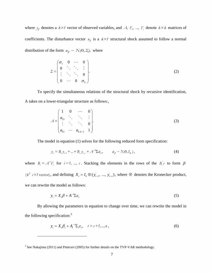
where yt denotes a k×1 vector of observed variables, and 1 sA, F , ..., F denote k×k matrices of
coefficients. The disturbance vector ut is a k×1 structural shock assumed to follow a normal
distribution of the form u ~ N(0,Σ),t where
1 0 00
00 0 k
σ
σ
Σ = . (2)
To specify the simultaneous relations of the structural shock by recursive identification,
A takes on a lower-triangular structure as follows:,
21
1 , 1
1 0 0
01k k k
a
a a −
A = . (3)
The model in equation (1) solves for the following reduced form specification:
1 ,tε− Σt 1 t -1 s t - sy = B y + ...+ B y + A kε N(0, I )t , (4)
where -1i iB = A F for i =1, ..., s . Stacking the elements in the rows of the '
iB s to form β
2 k s ×1 ( vector) , and defining ' '1( , ..., )t k t t sX I y y− −= ⊗ , where ⊗ denotes the Kronecker product,
we can rewrite the model as follows:
1t t ty X Aβ ε−= + Σ (5)
By allowing the parameters in equation to change over time, we can rewrite the model in
the following specification:3
1 ,t t t t t ty X Aβ ε−= + Σ t = s +1, ...,n , (6)
3 See Nakajima (2011) and Pimiceri (2005) for further details on the TVP-VAR methodology.
8
where the coefficients tβ , and the parameters tA and tΣ are all time varying. To model the
process for these time-varying parameters, Primiceri (2005) assumes the parameters in equation
(6) follow random-walk processes. Let '21 31 32 41 , 1( , , , , ..., )t k ka a a a a a −= denote a stacked vector
of the lower-triangular elements in tA and ( ,..., )1h h ht t kt ′= with 2logh jt jtσ= for j =1, ..., k ,
t = s +1, ..., n . Thus,
,1,1,1
β β β++
= ++= ++
t
t
t
utta a uatth h utt h
=
0 0 00 0 0
0, 0 0 0
0 0 0
ε
β β
Σ
Σ Σ
t t
t t
t t
Itu
Nua auh h
(7)
for t = s +1, ..., n , where ( , ),1 0 0Nsβ µβ βΣ+ ( , )1 0 0
a N as µ βΣ+ and ( , ).1 0 0h Ns h hµ Σ+
This methodology exploits the salient feature of the VAR model with time-varying
coefficients to estimate a three variable VAR model (interest rate, housing price index, and
equity price index), focusing on the dynamics of monetary policy (interest rate) adjustments in
relation with both housing and equity price adjustments. By allowing all parameters to vary over
time, this paper examines the assumption of parameter constancy for the VAR’s structural
shocks based on the standard recursive identification procedure known as the Choleski
decomposition. We achieve identification by imposing a lower triangular representation on the
matrix tA . The recursive ordering of the variables that proves consistent with the VAR based
empirical literature on monetary policy. That is, the interest rate comes first in the ordering and it
does not respond contemporaneously to housing and equity price shocks, while the housing price
react with a lag to equity price shocks. Thus, the housing price appears third in the ordering after
the equity (stock market) price.
9
3. Data
To examine the time-varying effects of housing and equity price shocks on the monetary policy,
we estimate the three-variable TVP-VAR model using annual data from 1890 to 2012. The
dataset comes primarily from the Online Data section of Robert Shiller’s website4 and includes
the real stock market price (RSP), the real housing price (RHP), and the short term interest rate
(R) commonly used as the monetary policy instrument. The data series on these variables,
however, only run to 2009 on Robert Shiller’s website. We update the data through 2012, using
the definition of the variables and sources outlined in the data files of Robert Shiller. The interest
rate variable appears to be stationary in levels. We transform the two asset-price variables into
their log-differenced form to ensure stationarity, given the existence of unit root in their level
forms.5 Further, for ease of comparison and interpretation, we standardize all variables using the
standard deviation. We choose a lag length of one based on the Akaike information criteria
applied to a stable constant parameter VAR. Since we convert the variables into their growth
rates and use one lag, the effective sample of our analysis starts in 1893.
4. Estimation results
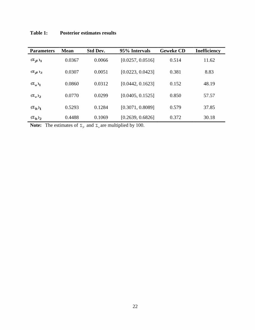
Table 1 reports the posterior estimates computed using the MCMC algorithm based on keeping
100,000 draws after 10,000 burn-ins.6 We perform diagnostic tests for convergence and
4 http://www.econ.yale.edu/~shiller/data.htm. 5 We use standard unit-root tests: Augmented-Dickey-Fuller (ADF)(1981), Phillips-Perron (PP)(1988), Dickey-Fuller with Generalised-Least-Squares-detrending (DF-GLS)(Elliott et al. , 1996), and the Ng-Perron modified version of the PP (NP-MZt)(2001) tests to confirm that the log-levels of the asset-price variables under consideration follow an integrated process of order 1 or I(1) processes. The unit-root tests are available on request from the authors. 6 The MCMC method assesses the joint posterior distributions of the parameters of interest based on certain prior probability densities that are set in advance. This paper implements the code of Nakajima (2011) by assuming the
following priors: (25, 0.01 ),IW IβΣ
2( ) (4, 0.02),Ga i−Σ
2( ) (4, 0.02),h Gi−Σ where 2( )a i
−Σ and 2( )h i−Σ are
10
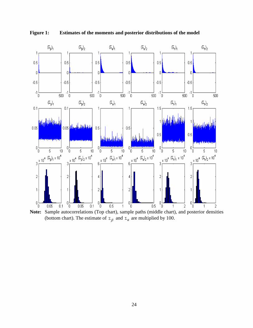
efficiency. The 95-percent credibility intervals include the estimates of the posterior means and
the convergence diagnostic (CD) statistics developed by Geweke (1992). We cannot reject the
null hypothesis of convergence to the posterior distribution at the conventional level of
significance. In addition, we also observe low inefficiency factors, confirming the efficiency (see
Figure 1) of the MCMC algorithm in replicating the posterior draws. These results indicate that
all three set of parameters ( βΣ t,Σ
ta ,Σth ), as described in equation (7), do change over time.
4.1. Estimates of the stochastic volatility
Besides the time varying structure of the parameters of interest ( βΣ t,Σ
ta ,Σth ), the volatility of
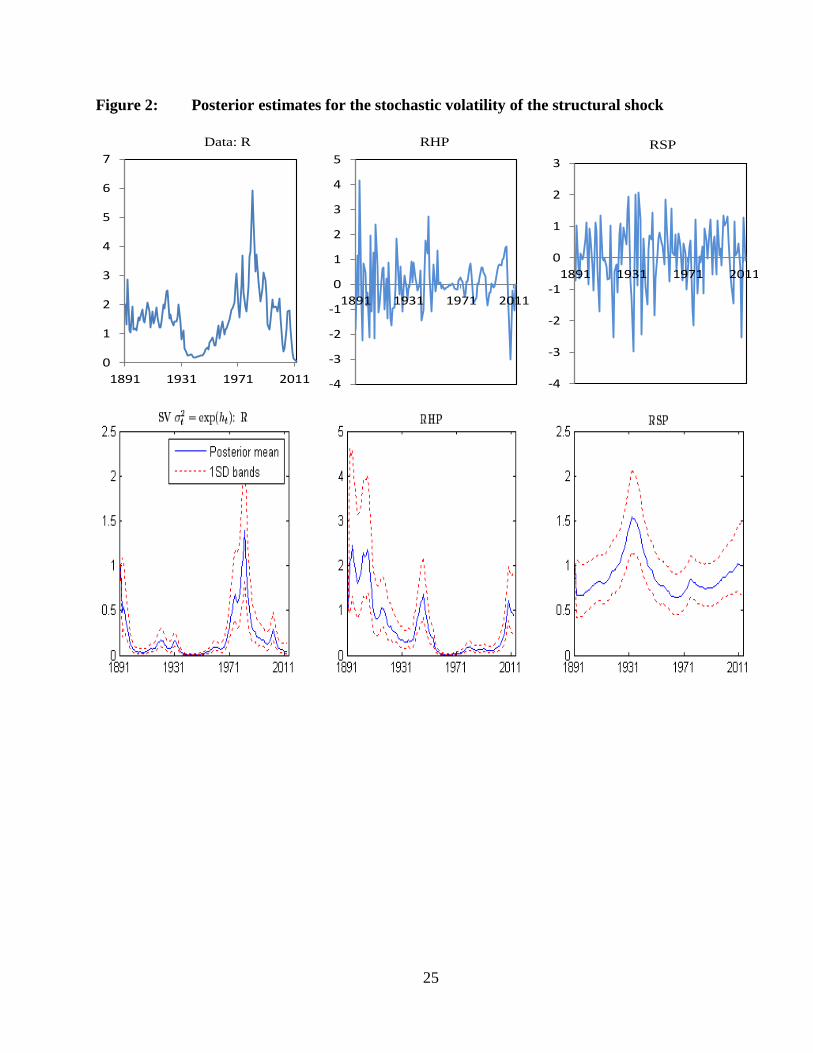
asset price shocks seems to match the evolution of monetary policy. Figure 2 plots the posterior
draws for each time series (top graphs) and the posterior estimates of the stochastic volatility
(bottom graphs). The pattern depicted by the volatility of the interest rate shocks seem
compatible with the historical evolution of the US monetary policy, at least from the
establishment of the Federal Reserves in 1914. For example, Lubik and Schorfheide (2004)
argue that the appointment of Paul Volker in 1979 as Federal Reserve Chairman marked a
watershed event for monetary policy. Before Volker, the Federal Reserve implemented a passive
monetary policy. That changes in 1979 and policy became much more aggressive. In their new
Keynesian monetary dynamic stochastic general equilibrium (DSGE) model, they discover that
the DSGE model exhibited indeterminacy and determinancy before and after 1979, respectively.
We observe that 1979 saw the peak in interest rate volatility.
the ith diagonal of elements of aΣ and hΣ , respectively. IW and G denote the inverse Wishart and the Gamma distributions, respectively. We use flat priors to set initial values of time-varying parameters such that:
00 0 0
µ µ µβ = = =a h and 10 .0 0 0βΣ = Σ = Σ = × Ia h
11
Meulendyke (1998) describes how US monetary policy evolved over time with various
changes reflecting different monetary policy objectives and their subsequent instruments. More
specifically, the low volatility observed prior to 1970s matches diverse monetary frameworks for
which interest rates did not play as important a role. Initially designed to control money and
credit through bank reserves coordination (1920s), the open market policy of the Federal Reserve
became more objective in the 1930s with the primarily goal of easing financial conditions
following the Great Depression prompted by the collapse of the stock market. During World War
II, monetary policy accommodated the war effort by holding down the cost of its financing in
1940s. The passage of the Treasury-Federal Reserve Accord of 1952 released the Federal
Reserve from the obligation of keeping the interest cost of the federal debt lower, which they did
during World War II. The Federal Reserve adopted the “bills only” policy in the 1950s, which
confined monetary policy to open markets operations in short maturity Treasury securities, bills,
and certificates of indebtedness with discount rate and reserve requirement changes used as
occasional supplements. Interestingly, the Federal Reserve adjusted margin requirements on
stock purchase occasionally to boost or dampen credit use (Meulendyke, 1998), thus reflecting
the observed increase in the volatility of the interest rate shocks.
In the late 1970s, US monetary policy moved from funds rate targeting to targeting
money and non-borrowed reserves (1979-1982) and subsequently to monetary and economic
objectives with borrowed reserves targets. This finally makes interest rates the key instrument in
the conduct of the US monetary policy, hence justifying the higher interest rate volatility towards
the end of the sample period. In relation to asset markets, the big increase in the volatility of the
interest rate in early 1980s coincides with the boom period of the two asset prices and, therefore,
the slowdown of both asset price volatilities. Though the relatively high volatility in both real
12
housing and real equity prices, we observe some interesting differences with regards to the
evolution of these two asset prices. The real housing price exhibits relative spikes between 1891
and 1951, although Shiller (2005) indicates the absence of any major real estate boom before
1940 and associates the observed decrease to World War I with the great influenza pandemic of
1918-19, the severe recession in 1920-21, and the high unemployment during the 1930s Great
Depression. Between the 1940s and 1960s, while interest rate volatility remains low, the real
housing price exhibits a relative increase in volatility whereas equity price volatility shows a
downward trend. After a long period of relative stability, the real housing price experiences new
increases in volatility toward the end of the sample, coinciding with the recent housing boom,
which began prior to the financial crisis and Great Recession in the late 2000s. In the second half
of 2000s, where peaks in the housing market followed peaks in the stock market with an average
lag of three years, we observe the same increase in asset prices and interest rate volatility. This
suggests the possibility of significant changes in the relationship between monetary policy and
asset prices over time, hence providing the rationale for using a TVP-VAR where the sources of
time variation include both the coefficients and the variance of the innovations.
Prior to World War II, monetary policy experienced three phases. The gold standard
operated prior to World War I where housing price volatility exceeded equity price volatility and
interest rate volatility followed a downward trend into the war period. During World War I the
newly charted Federal Reserve help to keep the interest cost of the federal debt low and we
observe relatively low interest rate volatility. After World War I, the world community tried to
return to the gold standard, which did not succeed. In the interwar period, housing price volatility
declined while equity price volatility rose reaching its peak in our sample during the Great
13
Depression. In addition, the nominal interest rate falls to its lowest point during the Great
Depression until the more recent financial crisis and Great Recession.
4.2 Evolution of the monetary policy
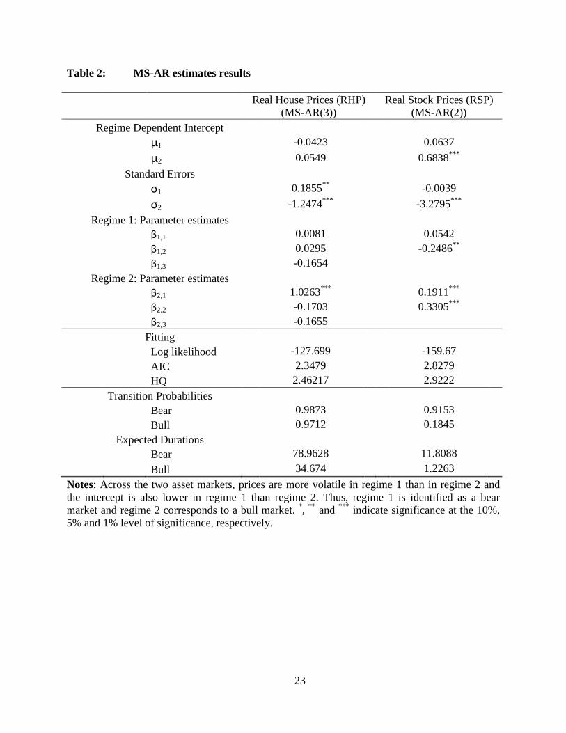
With the evidence of high volatilities in the dynamics of housing and equity prices, we also
explore the possibility of regime switches in the two financial markets, which may bring out
policy changes across regimes. We implement a Markov Switching Autoregressive (MS-AR)
model estimated for each asset category, which allows the identification of periods of high
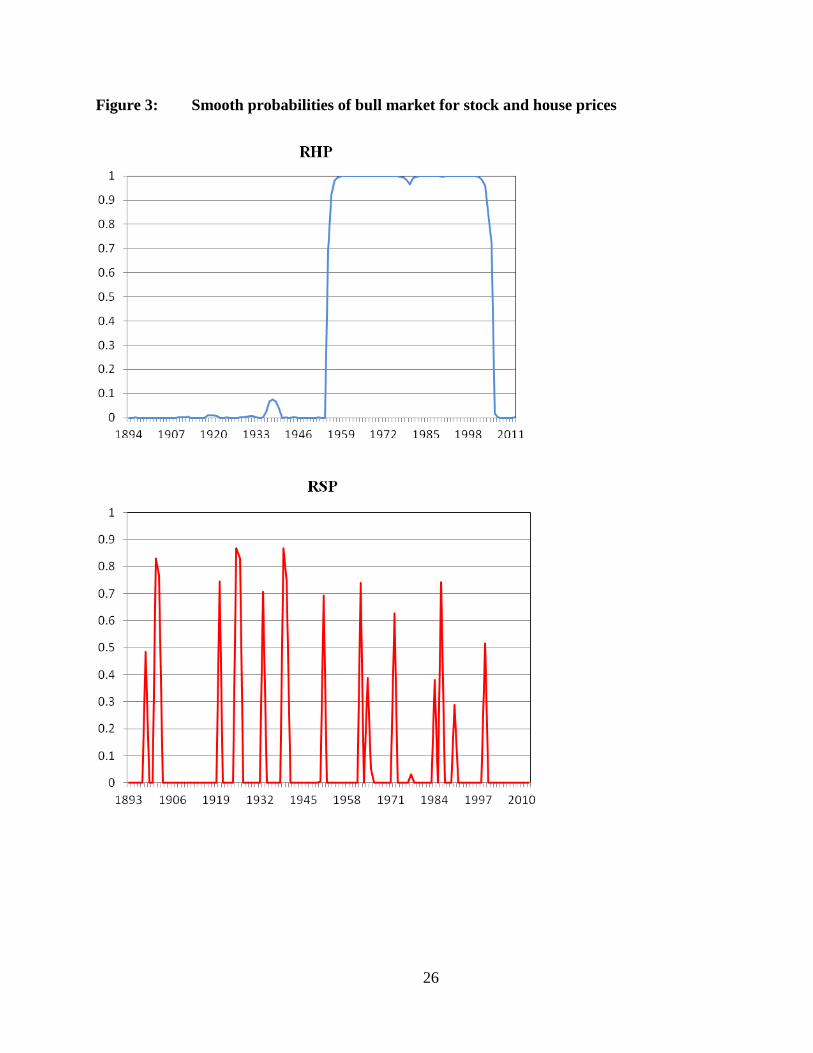
volatility (bear markets) and the period of low volatility (bull markets). Figure 3 plots the
smoothed probabilities for the bull market.7 Consistent with the 1998-2007 housing boom, the
housing market appears to enter the bull regime from 1960s to the second half of 2000s. Unlike
the housing market, the bull regimes in the stock market disseminate throughout the sample
period. Moreover, the patterns reveal different episodes of equity price booms identified by
Bordo and Wheelock (2004): the 1920s, 1930s, 1950s, 1960s, 1980s and 1990s.
In sum, the housing price exhibits one extended boom period from the mid-1950s through
the mid-2000s whereas the equity price exhibits a series of booms spread across the entire
sample period. The housing price boom achieved a probability of one for nearly its entire boom
period. The equity price boom never achieved a probability of a boom equal to one. Choosing the
equity price boom periods only for a probability of greater than 0.5, we identify 10 booms, early-
1900s, late-1910s, mid-1920s, mid- and late-1930s, early-1950s, early-1960s, early-1970s, mid-
1980s, and late-1990s.
7 Refer to the estimation results in Table 2 dealing with the identification of the bull and bear regimes in the housing and stock markets.
14
Another method of evaluating the evolution of monetary policy considers the impulse
response functions from the TVP-VAR model over selected horizons (we consider 1 to 6 years
ahead) at all points in time. This approach adds a third dimension to the analysis, hence allowing
the interpretation in terms of magnitude of the responses at each step and across regimes. We
begin by estimating the constant VAR impulse responses as a benchmark, which capture the
average levels of impulse response functions at all points in time over the sample period. Despite
the initial positive, but insignificant, response of equity prices to a monetary policy shock, which
lasts less than a year, the average effect of monetary policy on both asset prices appears negative
and generally insignificant throughout the time horizon (See panel A of Figure 4). The direction
of the effect corroborates the view in the monetary literature that an increase in the interest rate
likely lowers asset prices. The initial negative response of the housing price to a monetary policy
shock, however, does prove significant in year one and then becomes insignificant, but negative,
while rising to nearly zero in the remaining forecast horizon. Moreover, in terms of magnitude,
the housing price effect dominates the equity price effect of monetary policy in the short run (one
year), which contradicts the evidence from the TVP-VAR.
Unlike the constant VAR model, panel B of Figure 4 reveals a price puzzle at some
points in time with the positive response of house prices across different horizons. This puzzle
effect possibly emerges as a result of the lack of information contained in the parsimonious three
variables VAR (Korobilis, 2013). More interestingly, the magnitude of the housing price
response to a monetary policy shock exceeds in absolute value the response of the equity price
after 1980, which includes the boom period in the housing market. In absolute value, the
response of house prices to a one-standard-deviation change in the interest rate ranges from
between 1- to 6-percent compared to the response of the equity price, which lies between 0- and
15
1-percent. This contrasts with the relatively larger response of the equity price to an interest rate
shock prior to 1980, where the magnitude ranges between 1- to 5-percent in absolute value
against a 1- to 3-percent response of the housing price to a one-standard-deviation change in the
interest rate.
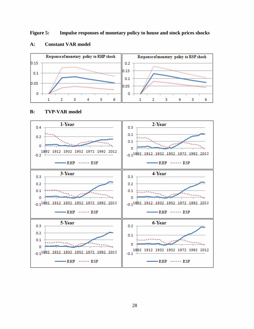
On the other hand, the positive feedback effects from both asset price shocks to monetary
policy prove consistent with previous studies (e.g., Demary, 2010; Ncube and Ndou, 2011;
Gupta et al., 2011; Peretti at al., 2012; Simo-Kengne et al., 2013) and indicate that the monetary
authorities tends to increase the interest rate as asset prices increase, giving a countercyclical
response of monetary policy to asset price adjustments. Results from the constant VAR model
show that the equity price exhibits the larger effect on monetary policy over the 6-year horizon
(see panel A of Figure 5).
Panel B of Figure 5, however, shows that monetary policy responds more strongly to
asset price shocks during its bull regime. That is, the housing price effect exceeds the equity
price effect after the early-1970s when the housing market experienced a bull regime. During
that period, the magnitude of the housing price effect oscillates between 10- to 20-percent across
horizons while a one-standard-deviation change in the equity price falls between 0- to 10-
percent. Similarly, the response of monetary policy to an equity price shock appears stronger
across horizons in the early part of the sample, where stock market booms saw more prominence.
Prior to 1970, a positive shock to the equity price leads to a 5- to 30- percent increase in interest
rate at all horizons against a positive response to a housing price shock ranging between 0- to 10-
percent.
16
5. Conclusion
The evolution of the US monetary policy experienced numerous modifications and adjustments
in response to various exogenous shocks of different sources. This paper evaluates a long dataset,
covering annual observations over the period of 1890-2012, to characterize the dynamic
relationship between asset prices and US monetary policy, as captured by the nominal interest
rate, based on a stochastic TVP-VAR approach and distinguishes between bull and bear regimes
to allow for more detailed interpretations. Moreover, we supplement the TVP-VAR approach
with a MS-AR model to identify switches between bear and bull regimes.
The empirical results substantiate a larger response of monetary policy to asset price
shocks during bull regimes, which correspond to a larger effect of interest rate shocks on asset
prices during boom periods. More specifically, monetary policy shocks exert a larger effect on
the housing price than the equity price after 1980 that corresponds to the bull regime in the
housing market. A higher response of the equity price to monetary policy shocks occurs prior
to1980.
We also find feedback effects of asset price shocks onto monetary policy, as measured by
the nominal interest rate. Monetary policy responds positively and more strongly to housing-
than equity-price shocks after the early-1970s, while monetary policy responds more strongly to
equity price shocks prior to early-1970s, where stock market booms exhibited more prominence.
Our findings support an important role for asset prices in the conduct of the monetary policy.
We explored the possibility of regime switches between bull and bear markets, using a
Markov Switching Autoregressive (MS-AR) model estimated for each asset category. We
identify periods of high volatility (bear markets) and low volatility (bull markets). The housing
market experiences an extended and continuous bull regime from the 1960s to the second half of
17
the 2000s. Unlike the housing market, the bull regimes in the stock market appear throughout the
sample period for relatively short periods of time.
Finally, our results indicate that the 1970s featured a dramatic change in the relationships
between asset prices and monetary policy. Chairman Volker took the leadership of the Federal
Reserve Board of Governors in 1979 as the macroeconomy transitioned from the Great Inflation
to the Great Moderation. The proponents of the good policy explanation of the Great Moderation
view Volker’s appointment as critical. That is, our findings support the view of Lubik and
Schorfheide (2004), who argue that the Volker’s appointment marked a watershed event for
monetary policy. Before Volker, the Federal Reserve implemented a passive monetary policy in
their view.
18
References: Ahmed, S., Levin, A., and Wilson, B. A., 2004. Recent U.S. macroeconomic stability: Good
policies, good practices, or good luck? Review of Economics and Statistics 86, 824-832. Aoki, K., Proudman, J., and Vlieghe, G., 2004. House prices, consumption and monetary policy:
a financial accelerator approach. Journal of Financial Intermediation 13, 414-435. Bernanke, B., and Gertler, M., 2001. Monetary policy and asset prices volatility. NBER working
paper 7559, Cambridge. Bhar, R., and Hamori, S., 2003. Alternative characterization of the volatility in the growth rate of
real GDP. Japan and the World Economy 15, 223-231. Blanchard, O., and Simon, J., 2001. The long and large decline in U.S. output volatility.
Brookings Papers on Economic Activity 32, 135-174. Boivin, J. 2005. Has US monetary policy changed? Evidence from drifting coefficients and real-
time data. NBER working paper 11314, Cambridge. Bordo, M.D., Dueker, M.J. and Wheelock, D.C. 2003. Aggregate price shocks and financial
stability: The United Kingdom 1796-1999. Explorations in Economic History, 40(4), 143-69.
Bordo, M. D., Dueker, M. J. and Wheelock, D. C. 2002. Aggregate price shocks and financial
stability: A historical analysis. Economic Inquiry, 40(4), 521-38. Bordo, M.D. and Wheelock, D.C. 2004. Monetary policy and asset prices: A look back at past
US stock market booms. NBER working paper 10704, Cambridge. Bordo, M.D. and Jeanne, O. 2002. Monetary policy and asset prices: Does benign neglect make
sense? International Finance, 5(2), 139-164. Borio, C. E. V., Kennedy, N., and Prowse, S. D., 1994. Exploring aggregate asset price
fluctuations across countries: Measurement, determinants, and monetary policy implications. Bank for International Settlements, BIS Economics Papers no. 40.
Case, K., Quigley, J., and Shiller, R., 2013. Wealth effects revisited: 1975-2012. NBER Working
Paper No. 18667. Demary, M. 2010. The interplay between output, inflation, interest rates and house prices.
International evidence Journal of Property Research, 27(1),1-17. Detken, C., and Smets, F., 2003. Asset price booms and monetary policy. manuscript, June.
19
Dickey, D. and Fuller, W. 1981. Likelihood ratio statistics for autoregressive time series with a unit root. Econometrica, 49, 1057-1072.
Elliott, G., Rothenberg, T.J. and Stock, J.H. 1996. Efficient tests for an autoregressive unit root.
Econometrica, 64 (4), 813-836. Filardo, A.J. 2000. Monetary policy and asset prices. Federal Reserve Bank of Kansas City
Economic Review, Third Quarter, 11-37. Gelain, P. and Lansing, K.J. 2013. House prices, expectations and time-varying fundamentals.
Federal Reserve Bank of San Francisco Working Paper 2013-03. Geweke, J., 1992. Evaluating the accuracy of sampling-based approaches to the calculation of
posterior moments. In Bernado, J. M., Berger, J. O., Dawid, A. P., and Smith, A. F. M., (eds), Bayesian Statistics. 4, 169-188, New York: Oxford University Press.
Gilchrist, S. and Leahy, J.V. 2002. Monetary policy and asset prices. Journal of Monetary
Economics, 49, 75-97. Goodhart, C. and Hofmann, B. 2001. Asset prices, financial conditions and the transmission of
monetary policy. Conference on Asset Prices, Exchange Rates, and Monetary Policy, Stanford University, March 2-3, 2001.
Green, G. D., 1971. The economic impact of the stock market boom and crash of 1929. In
Federal Reserve Bank of Boston, Consumer Spending and Monetary Policy: The Linkages, Monetary Conference, 189-220.
Guerrieri, L., and Iacoviello, M., 2013. Collateral constraints and macroeconomic asymmetries.
Mimeo, Boston College. Gupta, R., Jurgilas, M., Miller, S.M. and van Wyk, D. 2012. Financial market liberalization,
monetary policy and housing sector dynamics. International Business and Economics Research Journal, 11(1), 69-82.
Kim, C. J. and Nelson, C. R. (1999) Has the U.S. economy become more stable? A Bayesian
approach based on a Markov-Switching model of the business cycle, Review of Economics and Statistics 81, 1-10.
Kohn, D.L. 2009. Monetary policy and asset prices revisited. Cato Journal, 29(1), 31-44. Koop, G., Leon-Gonzalez, R. and Strachan, R.W. 2009. On the evolution of the monetary policy
transmission mechanism. Journal of Economic Dynamics and Control, 33, 997-1017. Korobilis, D. 2013. Assessing the transmission of monetary policy using time-varying parameter
dynamic factor models. Oxford Bulletin of Economics and Statistics, 75(2), 157-179.
20
Liu, Z., Wang, P., and Zha, T., 2013. Land-price dynamics and macroeconomic fluctuations. Econometrica, 81, 1147–1184.
Lubik, T.A. and Schorfheide, F. 2004. Testing for indeterminacy: An application to US monetary
policy. The American Economic Review, 94(1), 190-217. McConnell, M. M., and Perez-Quiros, G., 2000. Output fluctuations in the United States: What
has changed since the early 1980’s? American Economic Review 90, 1464-1476. Meulendyke, A. M., 1998. US monetary policy and financial markets. Federal Reserve Bank of
New York. Mian, A. R., Rao, K., and Sufi, A., 2013. Household balance sheets, consumption, and the
economic slump. Chicago Booth Research Paper no. 13-42, Fama-Miller Working Paper. Mills, T. C., and Wang, P., 2003. Have output growth rates stabilized? Evidence from the G-7
economies. Scottish Journal of Political Economy 50, 232-246. Mishkin, F. S., 2001. The transmission mechanism and the role of asset prices in monetary
policy. NBER working paper 8617,Cambridge. Mishkin, F. S., 2007. Housing and the Monetary Transmission Mechanism. Working Paper,
Finance and Economic Discussion Series, Federal Reserve Board. Nakajima, J., 2011. Time-varying parameter VAR model with stochastic volatility: An overview
of methodology and empirical applications. Monetary and Economic Studies, 107-142. Ncube, M. and Ndou, E. 2011. Monetary policy transmission, house prices and consumer
spending in South Africa: An SVAR approach. Working Paper 133, African Development Bank.
Peretti, V., Gupta, R. and Inglesi-Lotz, R.2012. Do house prices impact consumption and interest
rate in South Africa? Evidence from a Time Varying Vector Autoregressive model. Economics, Financial Markets and Management, 4, 101-120.
Phillips, P., and Perron, P., 1988. Testing for a unit root in time series regression. Biometrika 75,
335–346. Primiceri, G. E., 2005. Time varying structural vector autoregressions and monetary policy.
Review of Economic Studies 72, 821-852. Ng, S., and Perron, P., 2001. Lag lenth selection and the construction of unit root tests with good
size and power. Econometrica 69, 1519-1554. Shiller, R. J., 2005. Irrational exuberance. Princeton University Press, Princeton, New Jersey.
21
Simo-Kengne, B.D., Balcilar, M., Gupta, R., Aye, G.C. and Reid, M. 2013. Is the relationship between monetary policy and house prices asymmetric across bull and bear markets in South Africa? Evidence from a Markov-Switching Vector Autoregressive model. Economic Modelling, 32(1),161-171.
Sims, C.A. and Zha, T. 2006. Were regime switches in US monetary policy? The American
Economic Review, 96(1), 54-81. Stock, J. H., and Watson, M. W., 2003. Has the business cycle changed? Evidence and
explanations, Monetary Policy and Uncertainty: Adapting to a Changing Economy. Proceedings of symposium sponsored by Federal Reserve Bank of Kansas City, Jackson Hole, Wyo., 9-56.
Summers, P. M., 2005. What caused the Great Moderation? Some cross-country evidence.
Economic Review (Third Quarter), Federal Reserve Bank of Kansas City, 5-32. Zhou, X., And Carroll, C. D., 2012. Dynamics of wealth and consumption: new and improved
measures for U.S. states. The B.E. Journal of Macroeconomics, 12, 1-44.
22
Table 1: Posterior estimates results
Parameters Mean Std Dev. 95% Intervals Geweke CD Inefficiency
( )1βΣ 0.0367 0.0066 [0.0257, 0.0516] 0.514 11.62
( )2βΣ 0.0307 0.0051 [0.0223, 0.0423] 0.381 8.83
( )1aΣ 0.0860 0.0312 [0.0442, 0.1623] 0.152 48.19
( )2aΣ 0.0770 0.0299 [0.0405, 0.1525] 0.850 57.57
( )1hΣ 0.5293 0.1284 [0.3071, 0.8089] 0.579 37.85
( )2hΣ 0.4488 0.1069 [0.2639, 0.6826] 0.372 30.18 Note: The estimates of βΣ and aΣ are multiplied by 100.
23
Table 2: MS-AR estimates results
Real House Prices (RHP)
(MS-AR(3)) Real Stock Prices (RSP)
(MS-AR(2)) Regime Dependent Intercept
μ1 -0.0423 0.0637 μ2 0.0549 0.6838***
Standard Errors σ1 0.1855** -0.0039 σ2 -1.2474*** -3.2795***
Regime 1: Parameter estimates β1,1 0.0081 0.0542 β1,2 0.0295 -0.2486** β1,3 -0.1654
Regime 2: Parameter estimates β2,1 1.0263*** 0.1911*** β2,2 -0.1703 0.3305*** β2,3 -0.1655
Fitting Log likelihood -127.699 -159.67 AIC 2.3479 2.8279 HQ 2.46217 2.9222
Transition Probabilities Bear 0.9873 0.9153 Bull 0.9712 0.1845
Expected Durations Bear 78.9628 11.8088 Bull 34.674 1.2263 Notes: Across the two asset markets, prices are more volatile in regime 1 than in regime 2 and the intercept is also lower in regime 1 than regime 2. Thus, regime 1 is identified as a bear market and regime 2 corresponds to a bull market. *, ** and *** indicate significance at the 10%, 5% and 1% level of significance, respectively.
24
Figure 1: Estimates of the moments and posterior distributions of the model
Note: Sample autocorrelations (Top chart), sample paths (middle chart), and posterior densities
(bottom chart). The estimate of Σβ and aΣ are multiplied by 100.
25
Figure 2: Posterior estimates for the stochastic volatility of the structural shock
0
1
2
3
4
5
6
7
1891 1931 1971 2011
Data: R
-4
-3
-2
-1
0
1
2
3
4
5
1891 1931 1971 2011
RHP
-4
-3
-2
-1
0
1
2
3
1891 1931 1971 2011
RSP
26
Figure 3: Smooth probabilities of bull market for stock and house prices

27
Figure 4: Impulse responses of house and stock prices to monetary policy shock A: Constant VAR model
B: TVP-VAR model
28
Figure 5: Impulse responses of monetary policy to house and stock prices shocks A: Constant VAR model
B: TVP-VAR model