Eo

KP1

a

A

R

R

2

A

P

K

B

V

F

C

F

1

MtiMpcaR

0d

e c o l o g i c a l m o d e l l i n g 2 1 0 ( 2 0 0 8 ) 403–413

avai lab le at www.sc iencedi rec t .com

journa l homepage: www.e lsev ier .com/ locate /eco lmodel

volutionary cause of the vulnerabilityf insular communities

atsuhiko Yoshida ∗

opulation Ecology Section, Environmental Biology Division, National Institute for Environmental Studies,6-2 Onogawa, Tsukuba, Ibaraki 305-8506, Japan

r t i c l e i n f o

rticle history:

eceived 11 April 2007

eceived in revised form

6 July 2007

ccepted 7 August 2007

ublished on line 4 October 2007

eywords:

iological invasion

ulnerability of insular community

ood web model

omputer simulation

ood web structure

a b s t r a c t

Communities on oceanic islands are considered to be vulnerable to biological invasion. How-

ever, because the detailed structures of such communities have not yet been revealed, the

relationship between their vulnerability and structure is not clear. Because such communi-

ties evolved without biological invasion, they are expected to have structures different from

those of mainland communities, and this difference is expected to affect their vulnerability

to invasion. I conducted computer simulations based on a food web model and investigated

the difference in structure between mainland and insular model communities, the former

of which evolved with frequent invasion and the latter without invasion. In addition, by

conducting computer simulations of invasion of these model communities, I investigated

the relationship between community structure and vulnerability to biological invasion. The

insular model community evolved to have an unstable structure, in that a small number

of plant species supported a large number of animal species, and each species in the com-

munity had a small biomass. When a plant species invaded and disturbed the base of the

insular model community, many animal species relying on the plants easily became extinct.

In addition, when a carnivorous species invaded, animal species with small biomass tended

to become extinct. Community collapses caused by biological invasion occurred more fre-

quently in the insular model community than in the mainland model community. These

results indicated that those communities that evolved without invasion were vulnerable to

invasion. The available data on real insular communities suggest that some have reached

pred

1996; Williamson, 1996), because the communities on oceanic

the endangered state

. Introduction

ost recent species extinctions have occurred on islands, andhe majority are considered to have been caused by biologicalnvasion (e.g., Elton, 1958; Frankel and Soule, 1981; Loope and

ueller-Dombois, 1988). Therefore, insular communities—inarticular oceanic island communities—are considered espe-

ially vulnerable to biological invasion (Elton, 1958; Frankelnd Soule, 1981; Savage, 1987; Washitani and Yahara, 1996;odda et al., 1999; Hasegawa, 1999; CDFWWF, 2002). The cause

∗ Tel.: +81 298 50 2443; fax: +81 298 50 2586.E-mail address: kyoshida@nies.go.jp.

304-3800/$ – see front matter © 2007 Elsevier B.V. All rights reserved.oi:10.1016/j.ecolmodel.2007.08.007

icted by this model.

© 2007 Elsevier B.V. All rights reserved.

of this vulnerability has been discussed mainly in terms ofthe species on oceanic islands, which are considered sus-ceptible to invasive predators and competitors that havenever been encountered (Elton, 1958; Frankel and Soule, 1981;Savage, 1987; Rodda et al., 1999; Hasegawa, 1999; Clarke etal., 1984; Hadfield, 1986; Pimm, 1987; Washitani and Yahara,

islands have evolved without invasion (Elton, 1958; MacArthurand Wilson, 1967; Wagner and Funk, 1995; Grant, 1998; Chiba,2002).

i n g

404 e c o l o g i c a l m o d e l l

Because of this unique evolutionary history, insularcommunities may have structures different from those ofmainland communities, and if so, this difference in com-munity structure may affect the vulnerability to biologicalinvasion. In particular, there is an urgent need to deter-mine whether communities on oceanic islands can easilybe collapsed by slight disturbances (e.g., a single invasion).However, this subject has scarcely been touched on, becausethe detailed community structures of such insular communi-ties are not yet known, although those of several mainlandcommunities (e.g., Little Rock Lake: Martinez, 1991; the Hiurarocky intertidal community: Hori and Noda, 2001; TuesdayLake: Cohen et al., 2003) have been well investigated. Simi-larly, datasets for precisely investigated communities do notinclude data on community (e.g., Dunne et al., 2002; Broseet al., 2005), with the exception of the St. Martin Islands(Goldwasser and Roughgarden, 1993); moreover, there havebeen problems resolving the taxonomic classification of thedata for these islands, as discussed below.

Elton (1958) once stated that insular communities are vul-nerable to invasion because they have simple structures. It istrue that limited numbers of higher taxonomic groups existon oceanic islands (this is well known as disharmony: e.g.,Carloquist, 1974), and large carnivorous animals are oftenabsent (e.g., Elton, 1958; Carloquist, 1974). However, some ofthe taxonomic groups on oceanic islands have diversified intonumerous endemic species as a result of long-term evolution(Darwin, 1859; Wagner and Funk, 1995; Grant, 1998; Chiba,2002). Some insular communities consequently have veryhigh species diversity (e.g., Galapagos, Hawaii, Ogasawara). Insuch insular communities, complex interaction networks canbe expected to have developed, meaning that Elton’s (1958)statement does not apply to these insular communities. Inaddition, such complicated systems can exhibit unexpectedbehavior (e.g., sudden collapse by a slight disturbance).

Here, I conducted computer simulations based on a newfood web model and investigated the differences in structurebetween mainland and insular model communities, the for-mer of which evolved with frequent invasion and the latterwithout invasion. In addition, by conducting computer simu-lations of invasion of these model communities, I investigatedthe relationship between community structures and vulnera-bility to biological invasion.

2. Method

2.1. Food web model

I used a new food web model developed by modifying myprevious model (Yoshida, 2002, 2003, 2006a,b). In this modifica-tion, I introduced the rate of energy exchange in predation anddivided animals into herbivores, carnivores, and omnivores(see below).

In this model, a food web is represented by the followingmulti-dimensional Lotka–Volterra equation:

dMi

dt= eMi

⎛⎝ri +

n∑j=1

aijMj

⎞⎠ , (1)

2 1 0 ( 2 0 0 8 ) 403–413

where Mi and Mj are the total biomass of species i and j, respec-tively; e is the rate of energy exchange; ri is the intrinsic growthrate of species i; n is the number of species in the community;and aij is the effect of species j on species i. The actual calcu-lation is done by using the Euler method with a step size of0.001, and 1000 times the step size is defined as one time step.As a result of the calculation, if the total biomass of a speciesbecomes smaller than the individual body size of the species(w: the biomass of one individual of the species), the speciesbecomes extinct. In the initial setting, the value of w is ran-domly chosen for each species from the interval [0,0.003], andthe initial biomass of a species is set at 0.1.

In the initial state, the model community consists of 50animal and 50 plant species. Each of the 100 initial species isa founder of a clade, which is defined as a group of speciesderived from a common founder species. Each clade in themodel community is phylogenetically independent of the oth-ers. The value of the intrinsic growth rate (r) of a plant speciesis randomly chosen from the interval [0,2.0], reflecting thefact that plant species conduct primary production. Animalspecies are assumed to have a negative value of r, representingthe fact that animal species cannot survive without feedingon other species. The manner of setting r for animal speciesis mentioned below (Section 2.3).

2.2. Inter-specific interactions

In the model community, a predator species feeds on a preyspecies if the character of the prey meets the feeding prefer-ence of the predator. The character of the prey is described byan array of 10 D elements, and the feeding preference of thepredator is described by an array of 10 A elements. Whethera predatory species i feeds on a prey species j is judged bycounting the number of Dj elements that satisfy the followingcondition:

Ai[k] − Pi < Dj[k] < Ai[k] + Pi, (2)

where Pi is the range of feeding preference of species i, andAi[k] and Dj[k] are the kth elements of A of species i and Dof species j, respectively. If the number of elements of Dj sat-isfying the above condition is larger than a random numberchosen from the interval [0,10.0], then species i can feed onspecies j; that is, aij > 0. In the initial setting, the value of aij

is randomly chosen from [0,0.2], and aji, which is the effect ofspecies j on species i, is set to −aij.

In the current model, each element of D and A is randomlychosen from the interval [0,100.0]. The range of feeding pref-erence (P) is randomly chosen from the interval [0,10.0] (themean value of P is 5). Thereby, the probability that Dj[k] satis-fies the above condition is 0.1. In other words, one of the valueof Dj is expected to satisfy the condition. Therefore, the prob-ability that species i feeds on species j is 0.1. If the intervalfor choosing the value of P is narrowed, the connectance inthe food webs decreases, and the species diversity increases(Yoshida, 2002, 2003).

Because predators are usually larger than their prey in nat-ural communities (Vezina, 1985; Warren and Lawton, 1987;Cohen et al., 1993; Pahl-Wostl, 1997; Neubert et al., 2000;Jennings et al., 2001; Brose et al., 2005), this relationship was

g 2 1

fistT

drphge

D

wcdtscisss

ipmpsrpi

a

2c

Iabrtsfr

r

mTss

rcp

tion between the new species and a predator of the ancestor is

e c o l o g i c a l m o d e l l i n

xed as a rule in the present model. On the other hand, animalpecies can feed on plant species regardless of this assump-ion. In the model, carnivorous plants are not considered.hus, aij for plant i cannot be positive.

In the real world, neighboring plant species often hin-er each other’s growth through competition for light, soilesources, and germination sites, for example. I assumed thatlant species tend to hinder each other’s growth when theyave similar characters. Whether plant species a hinders therowth of plant species b is judged by counting the number oflements of Db satisfying the following condition:

a[k] − Ca < Db[k] < Da[k] + Ca, (3)

here C is the sensitivity to competition and is randomlyhosen from the interval [2.0,10.0], the range of which isetermined on the basis of the same concept by whichhe predator–prey interactions mentioned above were con-tructed. If the number of elements of Dj satisfying the aboveondition is larger than a random number chosen from thenterval [0,10.0], then species a hinders the growth of plantpecies b (aba < 0). Then, the value of aba is then randomly cho-en from [−0.2,0]. The value of aab, which is the effect of plantpecies b on species a, is determined independently of aba.

Diagonal elements of the interaction matrix aii representntra-specific competition coefficients. Generally speaking,lant species with a large intrinsic growth rate (r) produceany seeds, and the seeds are distributed near their parent

lant. Consequently, such species suffer from severe intra-pecific competition. In this model, plant species with largevalues are assumed to suffer from severe intra-specific com-etition (Yoshida, 2003). Then, if species i is a plant species, aii

s calculated by the following equation:

ii = −0.3 − ri

4.0× 0.7. (4)

.3. Intrinsic growth rate and intra-specificompetition of animal species

n the model, animal species with larger body sizes have andvantage in that they can feed on a potentially larger num-er of prey species than can smaller animals. However, theyequire large amounts of food. To search for prey, they haveo move their heavy bodies over long distances. Thus, animalpecies are assumed to consume large amounts of energy ineeding on other species. In this model, the intrinsic growthate of animal species is simply defined as follows:

i = −0.15 − wi

0.03× 0.35, (5)

This assumption is not always adopted to endothermic ani-als, but is adopted to ectothermic ones (Begon et al., 1996).

his equation assumes that a large animal species with a bodyize of 0.03–10 times the upper limit body size of the initialetting—loses half of its biomass in a time step.

Larger animals generally need much food and larger homeanges than do smaller ones (Palomares and Caro, 1999) and,onsequently, they experience more severe intra-specific com-etition than do smaller ones. Then, aii of animal species is set

0 ( 2 0 0 8 ) 403–413 405

by the following equation:

aii = −0.15 − wi

0.03× 0.35. (6)

This equation assumes that the value of aii of a large animalspecies with a body size of 0.03 is 0.5.

As frequently seen in such models, constants do notdepend on the actual values measured in the real world. Theconstants in Eqs. (5) and (6) are arbitrarily set. For simplicity,this model does not incorporate detailed assumptions defin-ing the forms of equations and the intensities of the energyloss (r) and the intra-specific competition (aii). Therefore, inthis model, the simplest form of equations representing thepenalty incurred by having a large body size is adopted, anda half of the penalty loading is assigned to r and the otherhalf is assigned to aii. This is the reason why both equationshave the same form. If the absolute value of the first term inthe equations is decreased, the loss of biomass of the animalspecies decreases. As a result, the probability of extinction ofthe animal species decreases. The second term influences theevolution of body size. If the denominator is increased, largerbody size is easily evolved (Yoshida, 2006b).

2.4. Evolution of model communities

In the model, a community is evolved via the evolution ofspecies. At every 100 steps, a new species is derived from arandomly chosen species in the model community. The totalbiomass of the new species is set to 5% of that of its ancestorspecies. Variables of the new species are set by adding smallvalues (slight mutations) to those of its ancestor. Values aregiven for the variables by random numbers drawn from Gaus-sian distributions with a mean of 0. The standard deviations ofthe Gaussian distributions are based on the evolutionary rate(E) of the ancestor: E for each element of A and D, 0.3E for P,0.1E for r, 0.1E for E, and 0.0003E for w. In the initial setting, thevalue of E is drawn from a Gaussian distribution with mean 1.0and standard deviation 0.1. These standard deviations are setnot to exceed 10% of the maximum of each variable. Gradualevolution is thereby realized in the model.

Inter-specific interactions of the new species are decidedby adding slight mutations to those of its ancestor species.When the new species is judged to feed on one of the prey ofthe ancestor species (using Eq. (3)), the coefficient of interac-tion between the new species and the prey is set by addingthe absolute value of a random number to that between theancestor and the prey. The random number is drawn from aGaussian distribution, with mean 0 and standard deviation0.1E of the new species. When a new species is judged notto feed on a prey of the ancestor, the coefficient of interac-tion between them is set by subtracting the absolute valueof a Gaussian random number (with mean 0 and standarddeviation 0.1E of the prey) from the coefficient of interactionbetween the ancestor and the prey. The coefficient of interac-

set in the same manner. Interactions between the new speciesand other species that are neither predator nor prey of theancestor are decided by the same manner as in the initialsetting.

i n g

406 e c o l o g i c a l m o d e l l

2.5. The rate of energy exchange and types of animalspecies

For their population growth, animal species can use a fractionof the biomass gained via predation. I assumed that an animalspecies that has a narrow range of feeding preference (P) andconsequently feeds on a limited number of prey species canutilize its prey species more effectively than a species witha wide range of feeding preference. Then, the rate of energyexchange, e, is defined as K/P, where K is a constant. The upperlimit of the rate of energy exchange is set to 1.0. There are nodata supporting the assumption that e is negatively related toP. However, the results of simulation without the assumptionshowed that the community was filled with generalist preda-tors and herbivores, indicating that the model without theassumption was not compatible with the real world in whichmany specialist predators and herbivores exist.

In addition, I advanced the previous model by dividinganimal species into herbivores (consuming plant species),carnivores (consuming animal species), and omnivores (con-suming both animal and plant species). These types of animalspecies were distinguished not only by their feeding propertiesbut also by the value of K. When omnivores feed on producerspecies, K is set to 1. When omnivores feed on animals, K isset to 2, because animals are efficient food resources (Begon etal., 1996). Herbivores and carnivores specialize for feeding onproducer species and animals, respectively; K for these typesof species is twice that for omnivores.

2.6. Construction of mainland and insular modelcommunities

Two types of community—insular and mainlandmodels—were constructed. The former represents com-munities that evolved without invasion on oceanic islands,and the latter represents communities that suffered fromfrequent invasion during their evolution in a locality withouta strict geographic barrier.

Both the mainland and insular model communities areconstructed via evolution over 100 000 steps (communitiesevolved via repeated evolution of species mentioned above).At every 500 steps in the course of evolution of a mainlandmodel community, a completely new species invades the com-munity and establishes a new clade. Invasions of a plant,omnivore, herbivore, and carnivore occur in that order. Vari-ables and interactions of the new founder species are given inthe same manner as in the initial setting. On the other hand,in the course of evolution of the insular model community,invasion never occurs. After evolution over 100 000 time steps,both the mainland and the insular model communities are leftfor 10 000 time steps without any operations, in order to voidthe effect of the last speciation. The resultant communitiesare called recipient communities.

2.7. Simulation of invasion

I used the insular and mainland models to conduct simula-tions of biological invasion. One species with a very smallbiomass (0.01: one-tenth of the biomass assigned to thespecies in the initial setting) invades a recipient community.

2 1 0 ( 2 0 0 8 ) 403–413

The parameter values for the invader, except for body size(w), are set in the same manner in the initial setting of themodel community. The value of w is randomly chosen fromthe interval [0,0.007]. The effect of invasion is observed for1000 time steps. After that the community is reset to the statebefore invasion, and the next species invades. In one set ofsimulations of invasion, each type of species (plant, omnivore,herbivore, and carnivore) invaded one recipient community 18times. This set of simulations is iterated 50 times for both theinsular and mainland models. Thus, a total of 3600 (4 × 18 × 50)invasions occurred in each model.

3. Results and discussion

3.1. Food web structure and reality of the modelcommunities

To determine the reality of the food web model, I first com-pared the mean values of topological parameters of theresultant mainland model community with those of 14 realcommunities (Pimm and Lawton, 1980; Baird and Ulanowics,1989; Warren, 1989; Hall and Raffaelli, 1991; Martinez, 1991;Polis, 1991; Goldwasser and Roughgarden, 1993; Huxham et al.,1996; Schneider, 1997; Yodzis, 1998; Christian and Luczkovich,1999; Martinez et al., 1999; Hori and Noda, 2001; Woodwardand Hildrew, 2001;). The degree of difference between real andmodel communities was measured by the manner introducedby Williams and Martinez (2000). The degree of the differenceof a given property is calculated as follows. First, calculate themean and standard deviation of the property of the model.Then, subtract the mean of the property of real communitiesfrom that of the model. Finally, divide the difference betweenthe means of the property in the real and model communitiesby the standard deviation of the property of the model. If thevalue of the degree of difference of a parameter is positive,then the mean value of the parameter of the model was largerthan that of real communities. If the value is 0, then there isno difference between the real and the model.

The degrees of difference of 8 parameters in the resultantmainland model community were smaller than 2 (Table 1).According to the criteria of Williams and Martinez (2000), themainland model reproduced some properties of real commu-nities successfully. The mainland model could not reproduceall the properties of real communities (Table 1), because incommunity models incorporating population dynamics it ismore difficult to control the topology of the resultant com-munity than in those without population dynamics (Yoshida,2006c). The most remarkable difference between this modeland real communities was in the ratio of animal to plantspecies (Table 1: animal/plant). This result indicates that toomany plant species existed in the model. The high value ofthe proportion of basal species (B) in the model also suggeststhis interpretation. In real communities, plant species tendto be highly lumped or resolved to a coarser taxonomic level(Briand and Cohen, 1984; Paine, 1988; Warren, 1989; Polis, 1991;

Martinez, 1993; Hall and Raffaelli, 1994), whereas all speciescan be distinguished in the model community. For example, inthe St. Martin Island food web (Goldwasser and Roughgarden,1993), basal species are very coarsely resolved as wood, roots,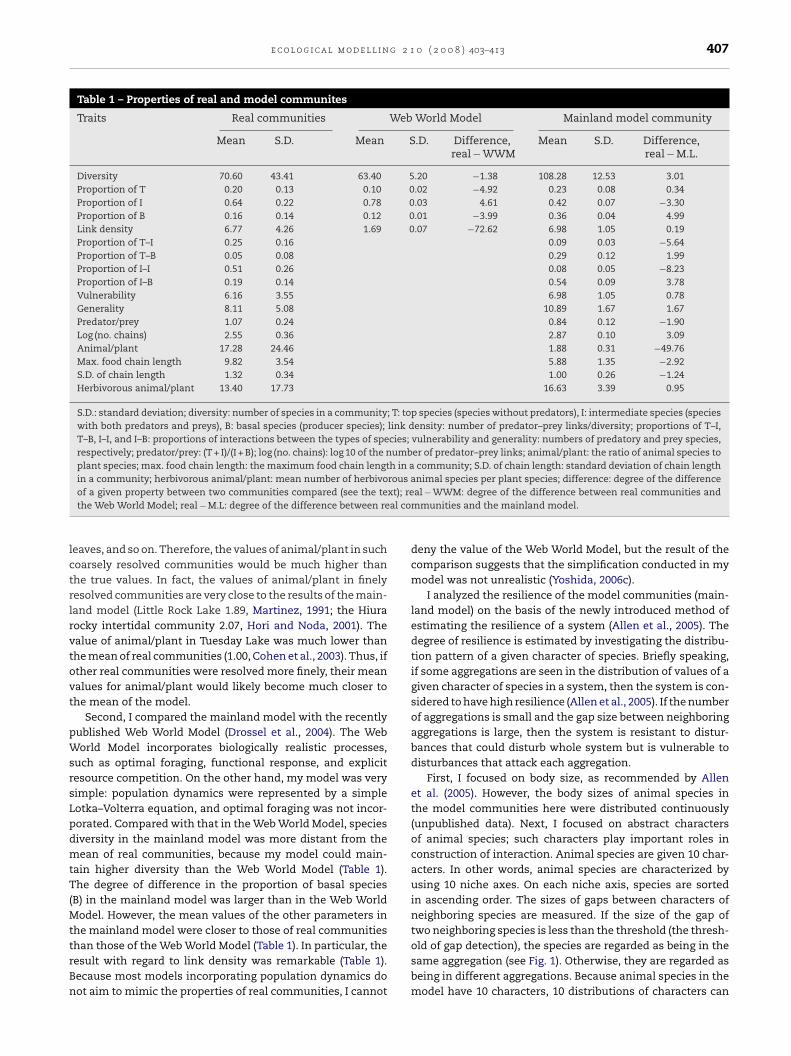

e c o l o g i c a l m o d e l l i n g 2 1 0 ( 2 0 0 8 ) 403–413 407

Table 1 – Properties of real and model communites

Traits Real communities Web World Model Mainland model community

Mean S.D. Mean S.D. Difference,real − WWM

Mean S.D. Difference,real − M.L.

Diversity 70.60 43.41 63.40 5.20 −1.38 108.28 12.53 3.01Proportion of T 0.20 0.13 0.10 0.02 −4.92 0.23 0.08 0.34Proportion of I 0.64 0.22 0.78 0.03 4.61 0.42 0.07 −3.30Proportion of B 0.16 0.14 0.12 0.01 −3.99 0.36 0.04 4.99Link density 6.77 4.26 1.69 0.07 −72.62 6.98 1.05 0.19Proportion of T–I 0.25 0.16 0.09 0.03 −5.64Proportion of T–B 0.05 0.08 0.29 0.12 1.99Proportion of I–I 0.51 0.26 0.08 0.05 −8.23Proportion of I–B 0.19 0.14 0.54 0.09 3.78Vulnerability 6.16 3.55 6.98 1.05 0.78Generality 8.11 5.08 10.89 1.67 1.67Predator/prey 1.07 0.24 0.84 0.12 −1.90Log (no. chains) 2.55 0.36 2.87 0.10 3.09Animal/plant 17.28 24.46 1.88 0.31 −49.76Max. food chain length 9.82 3.54 5.88 1.35 −2.92S.D. of chain length 1.32 0.34 1.00 0.26 −1.24Herbivorous animal/plant 13.40 17.73 16.63 3.39 0.95

S.D.: standard deviation; diversity: number of species in a community; T: top species (species without predators), I: intermediate species (specieswith both predators and preys), B: basal species (producer species); link density: number of predator–prey links/diversity; proportions of T–I,T–B, I–I, and I–B: proportions of interactions between the types of species; vulnerability and generality: numbers of predatory and prey species,respectively; predator/prey: (T + I)/(I + B); log (no. chains): log 10 of the number of predator–prey links; animal/plant: the ratio of animal species toplant species; max. food chain length: the maximum food chain length in a community; S.D. of chain length: standard deviation of chain lengthin a community; herbivorous animal/plant: mean number of herbivorous animal species per plant species; difference: degree of the difference

xt); real co

lctrlrvtovt

pWsrsLpdmtT(MttrBn

of a given property between two communities compared (see the tethe Web World Model; real − M.L: degree of the difference between re

eaves, and so on. Therefore, the values of animal/plant in suchoarsely resolved communities would be much higher thanhe true values. In fact, the values of animal/plant in finelyesolved communities are very close to the results of the main-and model (Little Rock Lake 1.89, Martinez, 1991; the Hiuraocky intertidal community 2.07, Hori and Noda, 2001). Thealue of animal/plant in Tuesday Lake was much lower thanhe mean of real communities (1.00, Cohen et al., 2003). Thus, ifther real communities were resolved more finely, their meanalues for animal/plant would likely become much closer tohe mean of the model.

Second, I compared the mainland model with the recentlyublished Web World Model (Drossel et al., 2004). The Weborld Model incorporates biologically realistic processes,

uch as optimal foraging, functional response, and explicitesource competition. On the other hand, my model was veryimple: population dynamics were represented by a simpleotka–Volterra equation, and optimal foraging was not incor-orated. Compared with that in the Web World Model, speciesiversity in the mainland model was more distant from theean of real communities, because my model could main-

ain higher diversity than the Web World Model (Table 1).he degree of difference in the proportion of basal species

B) in the mainland model was larger than in the Web Worldodel. However, the mean values of the other parameters in

he mainland model were closer to those of real communities

han those of the Web World Model (Table 1). In particular, theesult with regard to link density was remarkable (Table 1).ecause most models incorporating population dynamics doot aim to mimic the properties of real communities, I cannot

al − WWM: degree of the difference between real communities andmmunities and the mainland model.

deny the value of the Web World Model, but the result of thecomparison suggests that the simplification conducted in mymodel was not unrealistic (Yoshida, 2006c).

I analyzed the resilience of the model communities (main-land model) on the basis of the newly introduced method ofestimating the resilience of a system (Allen et al., 2005). Thedegree of resilience is estimated by investigating the distribu-tion pattern of a given character of species. Briefly speaking,if some aggregations are seen in the distribution of values of agiven character of species in a system, then the system is con-sidered to have high resilience (Allen et al., 2005). If the numberof aggregations is small and the gap size between neighboringaggregations is large, then the system is resistant to distur-bances that could disturb whole system but is vulnerable todisturbances that attack each aggregation.

First, I focused on body size, as recommended by Allenet al. (2005). However, the body sizes of animal species inthe model communities here were distributed continuously(unpublished data). Next, I focused on abstract charactersof animal species; such characters play important roles inconstruction of interaction. Animal species are given 10 char-acters. In other words, animal species are characterized byusing 10 niche axes. On each niche axis, species are sortedin ascending order. The sizes of gaps between characters ofneighboring species are measured. If the size of the gap oftwo neighboring species is less than the threshold (the thresh-

old of gap detection), the species are regarded as being in thesame aggregation (see Fig. 1). Otherwise, they are regarded asbeing in different aggregations. Because animal species in themodel have 10 characters, 10 distributions of characters can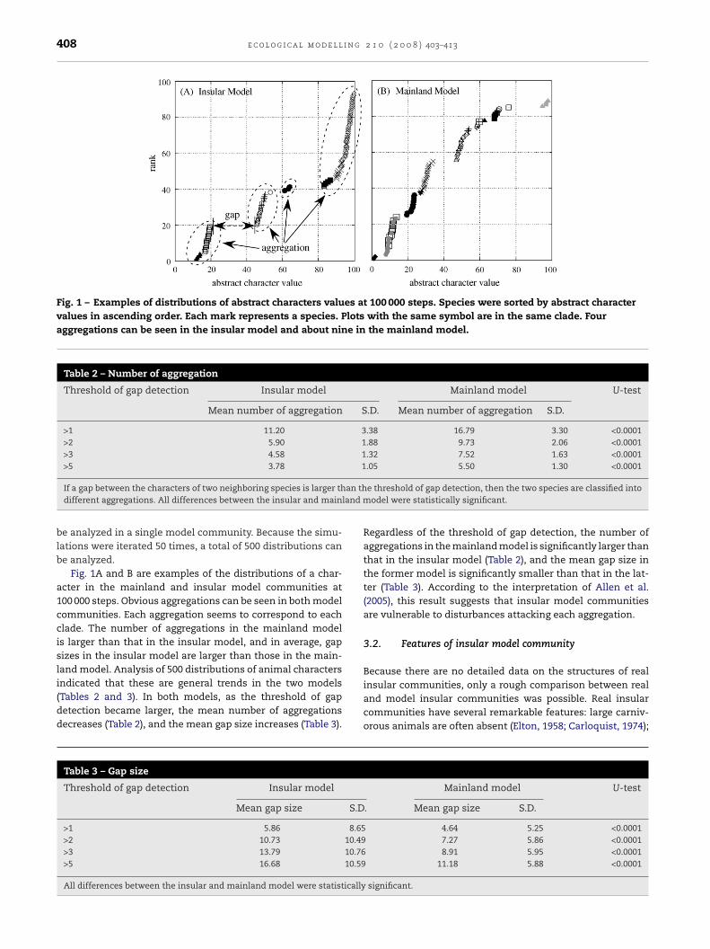

408 e c o l o g i c a l m o d e l l i n g 2 1 0 ( 2 0 0 8 ) 403–413

Fig. 1 – Examples of distributions of abstract characters values at 100 000 steps. Species were sorted by abstract charactervalues in ascending order. Each mark represents a species. Plots with the same symbol are in the same clade. Fouraggregations can be seen in the insular model and about nine in the mainland model.

Table 2 – Number of aggregation

Threshold of gap detection Insular model Mainland model U-test

Mean number of aggregation S.D. Mean number of aggregation S.D.

>1 11.20 3.38 16.79 3.30 <0.0001>2 5.90 1.88 9.73 2.06 <0.0001>3 4.58 1.32 7.52 1.63 <0.0001>5 3.78 1.05 5.50 1.30 <0.0001

an thland m

If a gap between the characters of two neighboring species is larger thdifferent aggregations. All differences between the insular and main

be analyzed in a single model community. Because the simu-lations were iterated 50 times, a total of 500 distributions canbe analyzed.

Fig. 1A and B are examples of the distributions of a char-acter in the mainland and insular model communities at100 000 steps. Obvious aggregations can be seen in both modelcommunities. Each aggregation seems to correspond to eachclade. The number of aggregations in the mainland modelis larger than that in the insular model, and in average, gapsizes in the insular model are larger than those in the main-land model. Analysis of 500 distributions of animal characters

indicated that these are general trends in the two models(Tables 2 and 3). In both models, as the threshold of gapdetection became larger, the mean number of aggregationsdecreases (Table 2), and the mean gap size increases (Table 3).

Table 3 – Gap size

Threshold of gap detection Insular model

Mean gap size S.D

>1 5.86 8.65>2 10.73 10.49>3 13.79 10.76>5 16.68 10.59

All differences between the insular and mainland model were statistically

e threshold of gap detection, then the two species are classified intoodel were statistically significant.

Regardless of the threshold of gap detection, the number ofaggregations in the mainland model is significantly larger thanthat in the insular model (Table 2), and the mean gap size inthe former model is significantly smaller than that in the lat-ter (Table 3). According to the interpretation of Allen et al.(2005), this result suggests that insular model communitiesare vulnerable to disturbances attacking each aggregation.

3.2. Features of insular model community

Because there are no detailed data on the structures of real

insular communities, only a rough comparison between realand model insular communities was possible. Real insularcommunities have several remarkable features: large carniv-orous animals are often absent (Elton, 1958; Carloquist, 1974);

Mainland model U-test

. Mean gap size S.D.

4.64 5.25 <0.00017.27 5.86 <0.00018.91 5.95 <0.0001

11.18 5.88 <0.0001

significant.

e c o l o g i c a l m o d e l l i n g 2 1 0 ( 2 0 0 8 ) 403–413 409

Table 4 – Properties of model communites

Traits Mainland model Insular model Ratio ins/main Test

Mean S.D. Mean S.D.

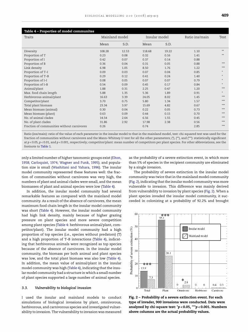
Diversity 108.28 12.53 118.68 19.22 1.10 **Proportion of T 0.23 0.08 0.32 0.16 1.41 **Proportion of I 0.42 0.07 0.37 0.14 0.88Proportion of B 0.36 0.04 0.31 0.05 0.88 ***Link density 6.98 1.05 8.50 1.76 1.22 ***Proportion of T–I 0.09 0.03 0.07 0.04 0.85 *Proportion of T–B 0.29 0.12 0.41 0.24 1.40 *Proportion of I–I 0.08 0.05 0.07 0.07 0.79 *Proportion of I–B 0.54 0.09 0.45 0.17 0.84 *Animal/plant 1.88 0.31 2.25 0.47 1.20 ***Max. food chain length 5.88 1.35 5.36 1.89 0.91 *Herbivorous animal/plant 16.63 3.39 24.05 8.02 1.45 ***Competitor/plant 3.70 0.75 5.80 1.34 1.57 ***Total plant biomass 23.34 3.97 15.69 4.82 0.67 ***Mean biomass (animal) 0.30 0.04 0.22 0.05 0.73 ***Mean biomass (plant) 0.63 0.09 0.44 0.15 0.70 ***No. of animal clades 14.54 2.64 6.56 1.55 0.45 ***No. of plant clades 31.86 2.92 17.98 2.38 0.56 ***Fraction of communities without carnivores 0.26 0.74 2.85 ***

Ratio (ins/main): ratio of the value of each parameter in the insular model to that in the mainland model, test: chi-squared test was used for the-testnum

o1tmtnb

rcmwhpappaibcwImlo

3

Isha

from vulnerability to invasion by plant species (Fig. 2). When aplant species invaded the insular model community, it suc-ceeded in colonizing at a probability of 92.2% and brought

fraction of communities without carnivores and the Mann–Whitney Uat p < 0.05, p < 0.01, and p < 0.001, respectively; competitor/plant: meanfootnote to Table 1.

nly a limited number of higher taxonomic groups exist (Elton,958; Carloquist, 1974; Wagner and Funk, 1995); and popula-ion size is small (Washitani and Yahara, 1996). The insular

odel community represented these features well: the frac-ion of communities without carnivores was very high, theumbers of plant and animal clades were small, and the meaniomasses of plant and animal species were low (Table 4).

In addition, the insular model community had severalemarkable features as compared with the mainland modelommunity. As a result of the absence of carnivores, the meanaximum food chain length in the insular model communityas short (Table 4). However, the insular model communityad high link density, mainly because of higher grazingressure on plant species and more severe competitionmong plant species (Table 4: herbivorous animal/plant, com-etitor/plant). The insular model community had a highroportion of top species (i.e., species without predators) (T)nd a high proportion of T–B interactions (Table 4), indicat-ng that herbivorous animals were recognized as top speciesecause of the absence of carnivores. In the insular modelommunity, the biomass per both animal and plant speciesas low, and the total plant biomass was also low (Table 4).

n addition, the mean value of animal/plant in the insularodel community was high (Table 4), indicating that the insu-

ar model community had a structure in which a small numberf plant species supported a large number of animal species.

.3. Vulnerability to biological invasion

used the insular and mainland models to conductimulations of biological invasions by plant, omnivorous,erbivorous, and carnivorous species and investigated vulner-bility to invasion. The vulnerability to invasion was measured

for all the other parameters; (*), (**), and (***): statistically significantber of competitors per plant species. For other abbreviations, see the

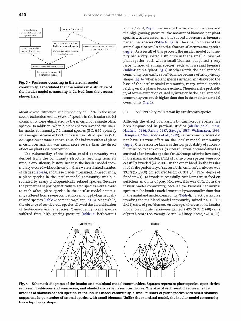
as the probability of a severe extinction event, in which morethan 5% of species in the recipient community are eliminatedby a single invasion.

The probability of severe extinction in the insular modelcommunity was twice that in the mainland model community(Fig. 2), indicating that the insular model community was morevulnerable to invasion. This difference was mainly derived

Fig. 2 – Probability of a severe extinction event. For eachtype of invader, 900 invasions were conducted. Data wereanalyzed by chi-square test: *p < 0.05, ***p < 0.001. Numbersabove columns are the actual probability values.

410 e c o l o g i c a l m o d e l l i n g

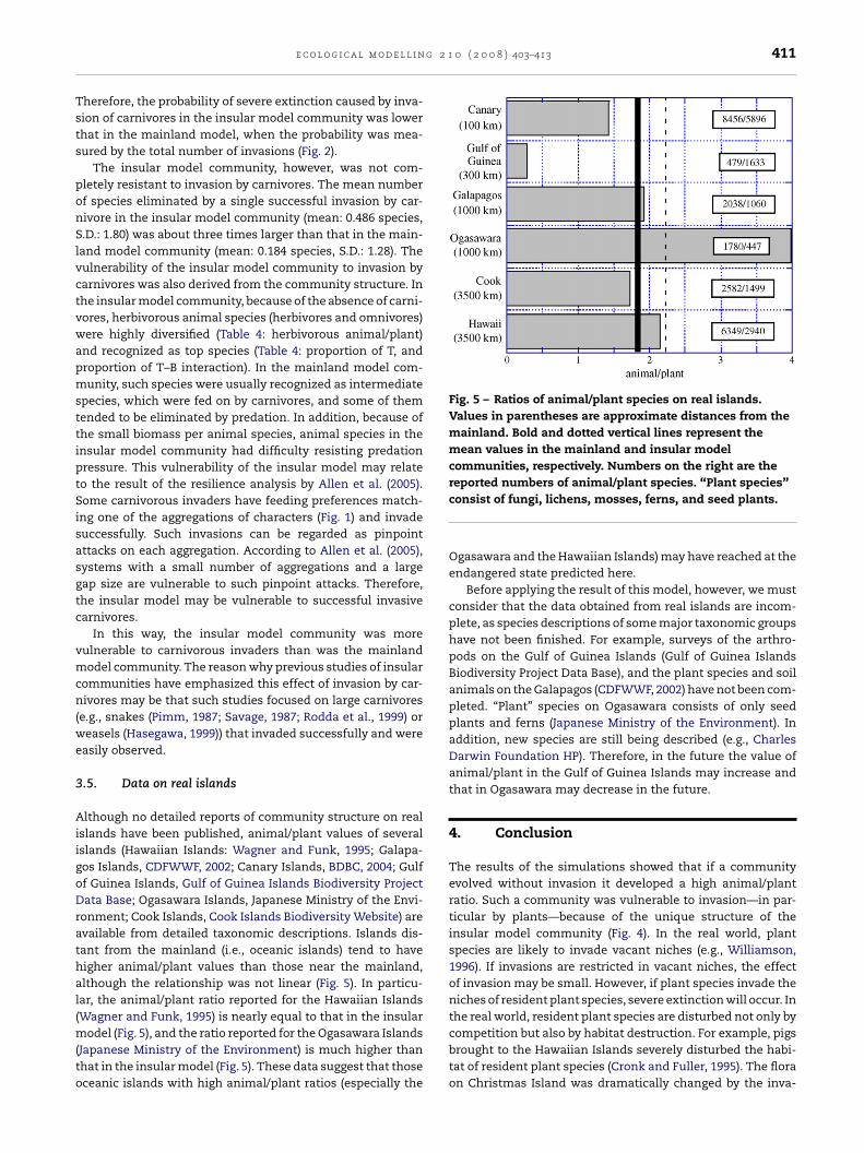
Fig. 3 – Processes occurring in the insular modelcommunity. I speculated that the remarkable structure of

the insular model community is derived from the processshown here.

about severe extinction at a probability of 55.1%. In the mostsevere extinction event, 36.2% of species in the insular modelcommunity were eliminated by the invasion of a single plantspecies. In addition, when a plant species invaded the insu-lar model community, 7.1 animal species (S.D. 6.61 species),on average, became extinct but only 1.47 plant species (S.D.2.40 species) became extinct. Thus, the indirect effect of plantinvasion on animals was much more severe than the directeffect on plants via competition.

The vulnerability of the insular model community wasderived from the community structure resulting from itsunique evolutionary history. Because the insular model com-munity evolved without invasion, there were a limited numberof clades (Table 4), and these clades diversified. Consequently,a plant species in the insular model community was sur-rounded by many phylogenetically related species. Becausethe properties of phylogenetically related species were similarto each other, plant species in the insular model commu-nity suffered from severe competition among phylogenetically

related species (Table 4: competitor/plant, Fig. 3). Meanwhile,the absence of carnivorous species allowed the diversificationof herbivorous animal species. Consequently, plant speciessuffered from high grazing pressure (Table 4: herbivorous

Fig. 4 – Schematic diagrams of the insular and mainland modelrepresent herbivores and omnivores, and shaded circles represenamount of biomass of each species. In the insular model commusupports a large number of animal species with small biomass.has a top-heavy shape.

2 1 0 ( 2 0 0 8 ) 403–413

animal/plant, Fig. 3). Because of the severe competition andthe high grazing pressure, the amount of biomass per plantspecies was decreased, and this caused a decrease in biomassper animal species (Table 4, Fig. 3). The small biomass of theanimal species resulted in the absence of carnivorous species(Fig. 3). As a result of this process, the insular model commu-nity had a very unstable structure in that a small number ofplant species, each with a small biomass, supported a verylarge number of animal species, each with a small biomass(Table 4: animal/plant: Fig. 4). In other words, the insular modelcommunity was easily set off-balance because of its top-heavyshape (Fig. 4): when a plant species invaded and disturbed thebase of the insular model community, many animal speciesrelying on the plants became extinct. Therefore, the probabil-ity of severe extinction caused by invasion in the insular modelcommunity was much higher than that in the mainland modelcommunity (Fig. 2).

3.4. Vulnerability to invasion by carnivorous species

Although the effect of invasion by carnivorous species hasbeen emphasized in previous studies (Clarke et al., 1984;Hadfield, 1986; Pimm, 1987; Savage, 1987; Williamson, 1996;Hasegawa, 1999; Rodda et al., 1999), carnivorous invaders didnot have a severe effect on the insular model community(Fig. 2). One reason for this was the low probability of success-ful invasion by carnivores. (Successful invasion was defined assurvival of an invader species for 1000 steps after its invasion.)In the mainland model, 27.2% of carnivorous species were suc-cessfully invaded (245/900). On the other hand, in the insularmodel, the probability of successful invasion of carnivores was19.2% (175/900) (chi-squared test: p < 0.001, �2 = 11.67, degree offreedom = 1). To invade successfully, carnivores must feed onsufficient amounts of prey. However, this was difficult in theinsular model community, because the biomass per animalspecies in the insular model community was smaller than thatin the mainland model community (Table 4). In fact, carnivores

invading the mainland model community gained 2.851 (S.D.:2.495) units of prey biomass on average, whereas in the insularmodel community carnivores gained 2.490 (S.D.: 2.248) unitsof prey biomass on average (Mann–Whitney U-test, p = 0.0135).

communities. Squares represent plant species, open circlest carnivores. The size of each symbol represents thenity, a small number of plant species with small biomassUnlike the mainland model, the insular model community

g 2 1 0 ( 2 0 0 8 ) 403–413 411

Tsts

ponSlvctvwapmsttiptSisasgtc

vmcn(we

3

AiigoDrathal(m(to

Fig. 5 – Ratios of animal/plant species on real islands.Values in parentheses are approximate distances from themainland. Bold and dotted vertical lines represent themean values in the mainland and insular modelcommunities, respectively. Numbers on the right are the

e c o l o g i c a l m o d e l l i n

herefore, the probability of severe extinction caused by inva-ion of carnivores in the insular model community was lowerhat in the mainland model, when the probability was mea-ured by the total number of invasions (Fig. 2).

The insular model community, however, was not com-letely resistant to invasion by carnivores. The mean numberf species eliminated by a single successful invasion by car-ivore in the insular model community (mean: 0.486 species,.D.: 1.80) was about three times larger than that in the main-and model community (mean: 0.184 species, S.D.: 1.28). Theulnerability of the insular model community to invasion byarnivores was also derived from the community structure. Inhe insular model community, because of the absence of carni-ores, herbivorous animal species (herbivores and omnivores)ere highly diversified (Table 4: herbivorous animal/plant)nd recognized as top species (Table 4: proportion of T, androportion of T–B interaction). In the mainland model com-unity, such species were usually recognized as intermediate

pecies, which were fed on by carnivores, and some of themended to be eliminated by predation. In addition, because ofhe small biomass per animal species, animal species in thensular model community had difficulty resisting predationressure. This vulnerability of the insular model may relateo the result of the resilience analysis by Allen et al. (2005).ome carnivorous invaders have feeding preferences match-

ng one of the aggregations of characters (Fig. 1) and invadeuccessfully. Such invasions can be regarded as pinpointttacks on each aggregation. According to Allen et al. (2005),ystems with a small number of aggregations and a largeap size are vulnerable to such pinpoint attacks. Therefore,he insular model may be vulnerable to successful invasivearnivores.

In this way, the insular model community was moreulnerable to carnivorous invaders than was the mainlandodel community. The reason why previous studies of insular

ommunities have emphasized this effect of invasion by car-ivores may be that such studies focused on large carnivores

e.g., snakes (Pimm, 1987; Savage, 1987; Rodda et al., 1999) oreasels (Hasegawa, 1999)) that invaded successfully and were

asily observed.

.5. Data on real islands

lthough no detailed reports of community structure on realslands have been published, animal/plant values of severalslands (Hawaiian Islands: Wagner and Funk, 1995; Galapa-os Islands, CDFWWF, 2002; Canary Islands, BDBC, 2004; Gulff Guinea Islands, Gulf of Guinea Islands Biodiversity Projectata Base; Ogasawara Islands, Japanese Ministry of the Envi-

onment; Cook Islands, Cook Islands Biodiversity Website) arevailable from detailed taxonomic descriptions. Islands dis-ant from the mainland (i.e., oceanic islands) tend to haveigher animal/plant values than those near the mainland,lthough the relationship was not linear (Fig. 5). In particu-ar, the animal/plant ratio reported for the Hawaiian IslandsWagner and Funk, 1995) is nearly equal to that in the insular

odel (Fig. 5), and the ratio reported for the Ogasawara IslandsJapanese Ministry of the Environment) is much higher thanhat in the insular model (Fig. 5). These data suggest that thoseceanic islands with high animal/plant ratios (especially the

reported numbers of animal/plant species. “Plant species”consist of fungi, lichens, mosses, ferns, and seed plants.

Ogasawara and the Hawaiian Islands) may have reached at theendangered state predicted here.

Before applying the result of this model, however, we mustconsider that the data obtained from real islands are incom-plete, as species descriptions of some major taxonomic groupshave not been finished. For example, surveys of the arthro-pods on the Gulf of Guinea Islands (Gulf of Guinea IslandsBiodiversity Project Data Base), and the plant species and soilanimals on the Galapagos (CDFWWF, 2002) have not been com-pleted. “Plant” species on Ogasawara consists of only seedplants and ferns (Japanese Ministry of the Environment). Inaddition, new species are still being described (e.g., CharlesDarwin Foundation HP). Therefore, in the future the value ofanimal/plant in the Gulf of Guinea Islands may increase andthat in Ogasawara may decrease in the future.

4. Conclusion

The results of the simulations showed that if a communityevolved without invasion it developed a high animal/plantratio. Such a community was vulnerable to invasion—in par-ticular by plants—because of the unique structure of theinsular model community (Fig. 4). In the real world, plantspecies are likely to invade vacant niches (e.g., Williamson,1996). If invasions are restricted in vacant niches, the effectof invasion may be small. However, if plant species invade theniches of resident plant species, severe extinction will occur. Inthe real world, resident plant species are disturbed not only by

competition but also by habitat destruction. For example, pigsbrought to the Hawaiian Islands severely disturbed the habi-tat of resident plant species (Cronk and Fuller, 1995). The floraon Christmas Island was dramatically changed by the inva-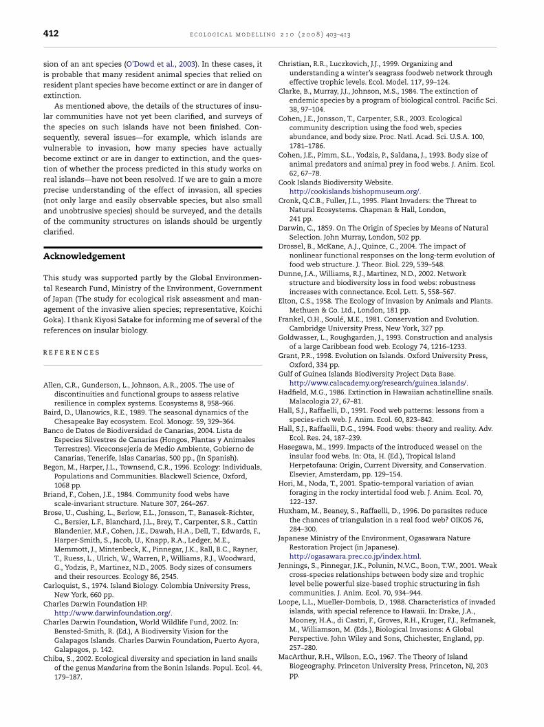

i n g

r

412 e c o l o g i c a l m o d e l l

sion of an ant species (O’Dowd et al., 2003). In these cases, itis probable that many resident animal species that relied onresident plant species have become extinct or are in danger ofextinction.

As mentioned above, the details of the structures of insu-lar communities have not yet been clarified, and surveys ofthe species on such islands have not been finished. Con-sequently, several issues—for example, which islands arevulnerable to invasion, how many species have actuallybecome extinct or are in danger to extinction, and the ques-tion of whether the process predicted in this study works onreal islands—have not been resolved. If we are to gain a moreprecise understanding of the effect of invasion, all species(not only large and easily observable species, but also smalland unobtrusive species) should be surveyed, and the detailsof the community structures on islands should be urgentlyclarified.

Acknowledgement

This study was supported partly by the Global Environmen-tal Research Fund, Ministry of the Environment, Governmentof Japan (The study for ecological risk assessment and man-agement of the invasive alien species; representative, KoichiGoka). I thank Kiyosi Satake for informing me of several of thereferences on insular biology.

e f e r e n c e s

Allen, C.R., Gunderson, L., Johnson, A.R., 2005. The use ofdiscontinuities and functional groups to assess relativeresilience in complex systems. Ecosystems 8, 958–966.

Baird, D., Ulanowics, R.E., 1989. The seasonal dynamics of theChesapeake Bay ecosystem. Ecol. Monogr. 59, 329–364.

Banco de Datos de Biodiversidad de Canarias, 2004. Lista deEspecies Silvestres de Canarias (Hongos, Plantas y AnimalesTerrestres). Viceconsejerıa de Medio Ambiente, Gobierno deCanarias, Tenerife, Islas Canarias, 500 pp., (In Spanish).

Begon, M., Harper, J.L., Townsend, C.R., 1996. Ecology: Individuals,Populations and Communities. Blackwell Science, Oxford,1068 pp.

Briand, F., Cohen, J.E., 1984. Community food webs havescale-invariant structure. Nature 307, 264–267.

Brose, U., Cushing, L., Berlow, E.L., Jonsson, T., Banasek-Richter,C., Bersier, L.F., Blanchard, J.L., Brey, T., Carpenter, S.R., CattinBlandenier, M.F., Cohen, J.E., Dawah, H.A., Dell, T., Edwards, F.,Harper-Smith, S., Jacob, U., Knapp, R.A., Ledger, M.E.,Memmott, J., Mintenbeck, K., Pinnegar, J.K., Rall, B.C., Rayner,T., Ruess, L., Ulrich, W., Warren, P., Williams, R.J., Woodward,G., Yodzis, P., Martinez, N.D., 2005. Body sizes of consumersand their resources. Ecology 86, 2545.

Carloquist, S., 1974. Island Biology. Colombia University Press,New York, 660 pp.

Charles Darwin Foundation HP.http://www.darwinfoundation.org/.

Charles Darwin Foundation, World Wildlife Fund, 2002. In:Bensted-Smith, R. (Ed.), A Biodiversity Vision for the

Galapagos Islands. Charles Darwin Foundation, Puerto Ayora,Galapagos, p. 142.

Chiba, S., 2002. Ecological diversity and speciation in land snailsof the genus Mandarina from the Bonin Islands. Popul. Ecol. 44,179–187.

2 1 0 ( 2 0 0 8 ) 403–413

Christian, R.R., Luczkovich, J.J., 1999. Organizing andunderstanding a winter’s seagrass foodweb network througheffective trophic levels. Ecol. Model. 117, 99–124.

Clarke, B., Murray, J.J., Johnson, M.S., 1984. The extinction ofendemic species by a program of biological control. Pacific Sci.38, 97–104.

Cohen, J.E., Jonsson, T., Carpenter, S.R., 2003. Ecologicalcommunity description using the food web, speciesabundance, and body size. Proc. Natl. Acad. Sci. U.S.A. 100,1781–1786.

Cohen, J.E., Pimm, S.L., Yodzis, P., Saldana, J., 1993. Body size ofanimal predators and animal prey in food webs. J. Anim. Ecol.62, 67–78.

Cook Islands Biodiversity Website.http://cookislands.bishopmuseum.org/.

Cronk, Q.C.B., Fuller, J.L., 1995. Plant Invaders: the Threat toNatural Ecosystems. Chapman & Hall, London,241 pp.

Darwin, C., 1859. On The Origin of Species by Means of NaturalSelection. John Murray, London, 502 pp.

Drossel, B., McKane, A.J., Quince, C., 2004. The impact ofnonlinear functional responses on the long-term evolution offood web structure. J. Theor. Biol. 229, 539–548.

Dunne, J.A., Williams, R.J., Martinez, N.D., 2002. Networkstructure and biodiversity loss in food webs: robustnessincreases with connectance. Ecol. Lett. 5, 558–567.

Elton, C.S., 1958. The Ecology of Invasion by Animals and Plants.Methuen & Co. Ltd., London, 181 pp.

Frankel, O.H., Soule, M.E., 1981. Conservation and Evolution.Cambridge University Press, New York, 327 pp.

Goldwasser, L., Roughgarden, J., 1993. Construction and analysisof a large Caribbean food web. Ecology 74, 1216–1233.

Grant, P.R., 1998. Evolution on Islands. Oxford University Press,Oxford, 334 pp.

Gulf of Guinea Islands Biodiversity Project Data Base.http://www.calacademy.org/research/guinea islands/.

Hadfield, M.G., 1986. Extinction in Hawaiian achatinelline snails.Malacologia 27, 67–81.

Hall, S.J., Raffaelli, D., 1991. Food web patterns: lessons from aspecies-rich web. J. Anim. Ecol. 60, 823–842.

Hall, S.J., Raffaelli, D.G., 1994. Food webs: theory and reality. Adv.Ecol. Res. 24, 187–239.

Hasegawa, M., 1999. Impacts of the introduced weasel on theinsular food webs. In: Ota, H. (Ed.), Tropical IslandHerpetofauna: Origin, Current Diversity, and Conservation.Elsevier, Amsterdam, pp. 129–154.

Hori, M., Noda, T., 2001. Spatio-temporal variation of avianforaging in the rocky intertidal food web. J. Anim. Ecol. 70,122–137.

Huxham, M., Beaney, S., Raffaelli, D., 1996. Do parasites reducethe chances of triangulation in a real food web? OIKOS 76,284–300.

Japanese Ministry of the Environment, Ogasawara NatureRestoration Project (in Japanese).http://ogasawara.prec.co.jp/index.html.

Jennings, S., Pinnegar, J.K., Polunin, N.V.C., Boon, T.W., 2001. Weakcross-species relationships between body size and trophiclevel belie powerful size-based trophic structuring in fishcommunities. J. Anim. Ecol. 70, 934–944.

Loope, L.L., Mueller-Dombois, D., 1988. Characteristics of invadedislands, with special reference to Hawaii. In: Drake, J.A.,Mooney, H.A., di Castri, F., Groves, R.H., Kruger, F.J., Refmanek,M., Williamson, M. (Eds.), Biological Invasions: A GlobalPerspective. John Wiley and Sons, Chichester, England, pp.

257–280.

MacArthur, R.H., Wilson, E.O., 1967. The Theory of IslandBiogeography. Princeton University Press, Princeton, NJ, 203pp.

g 2 1

M

M

M

N

O

P

P

P

P

P

P

R

S

S

e c o l o g i c a l m o d e l l i n

artinez, N.D., 1991. Artifacts or attributes? effects of resolutionon the Little Rock Lake food web. Ecol. Monogr. 61, 367–392.

artinez, N.D., 1993. Effects of resolution on food web structure.OIKOS 66, 403–412.

artinez, N.D., Hawkins, B.A., Dawah, H.A., Feifarek, B.P., 1999.Effects of sampling effort on characterization of food-webstructure. Ecology 80, 1044–1055.

eubert, M.G., Blumenshine, S.C., Duplisea, D.E., Jonsson, T.,Rashleigh, B., 2000. Body size and food web structure: testingthe equiprobability assumption and the cascade model.Oecologia 123, 241–251.

’Dowd, D.J., Green, P.T., Lake, P.S., 2003. Invasional ’meltdown’on an oceanic island. Ecol. Lett. 6, 812–817.

ahl-Wostl, C., 1997. Dynamic structure of a food web model:comparison with a food chain model. Ecol. Model. 100,103–123.

aine, R.T., 1988. Food webs: road maps of interactions or grist fortheoretical development? Ecology 69, 1648–1654.

alomares, F., Caro, T.M., 1999. Interspecific killing amongmammalian carnivores. Am. Nat. 153, 492–508.

imm, S.L., 1987. The snake that ate Guam. Trends Ecol. Evol. 2,293–295.

imm, S.L., Lawton, J.H., 1980. Are food webs divided intocompartments? J. Anim. Ecol. 49, 879–898.

olis, G.A., 1991. Complex trophic interactions in deserts: anempirical critique of food web theory. Am. Nat. 138, 123–155.

odda, G.H., Fritts, T.H., McCoid, M.J., Campbell, E.W.I., 1999. Anoverview of the biology of the brown treesnake (Boigairregularis), a costly introduced pest on pacific islands. In:Rodda, G.H., Sawai, Y., Chiszar, D., Tanaka, H. (Eds.), ProblemSnake Management: the Habu and the Brown Treesnake.Comstock Publishing Associates, Ithaca, pp. 44–80.

atake, K., Cai, Y., 2005. Paratya boninensis, a new species offreshwater shrimp (Crustacea: Decapoda: Atyidae) fromOgasawara, Japan. Proc. Biol. Soc. Washington 118, 306–311.

atake, K., Kuranishi, R.B., Ueno, R., 2005. Caddisflies (Insecta:Trichoptera) collected from the Bonin Islands and the IzuArchipelago, Japan. In: Proceedings of the 11th InternationalTrichoptera Symposium. Tokai University Press, Kanagawa,pp. 371–381.

0 ( 2 0 0 8 ) 403–413 413

Savage, J.A., 1987. Extinction of an island forest avifauna by anintroduced snake. Ecology 68, 660–668.

Schneider, D.W., 1997. Predation and food web structure along ahabitat duration gradient. Oecologia 110, 567–575.

Vezina, A.F., 1985. Empirical relationship between predator andprey size among terrestrial vertebrate predators. Oecologia 67,555–565.

Wagner, W.L., Funk, V.A., 1995. Hawaiian Biogeography.Smithsonian Institution Press, Washington, 467 pp.

Warren, P.H., 1989. Spatial and temporal variation in thestructure of a freshwater food web. OIKOS 55,299–311.

Warren, P.H., Lawton, J.H., 1987. Invertebrate predator–prey bodysize relationship: an explanation for upper triangular foodwebs and patterns in food web structure? Oecologia 74,231–235.

Washitani, I., Yahara, T., 1996. An Introduction to ConservationBiology: from Gene to Landscape (in Japanese). Bun-ichi SoGoShyuppan, Co., Ltd., Tokyo, 270 pp.

Williams, R.J., Martinez, N.D., 2000. Simple rules yield complexfood webs. Nature 404, 180–183.

Williamson, M., 1996. Biological Invasions. Chapman & Hall,London, 244 pp.

Woodward, G., Hildrew, A.G., 2001. Invasion of a stream food webby a new top predator. J. Anim. Ecol. 70, 273–288.

Yodzis, P., 1998. Local trophodynamics and the interaction ofmarine mammals and fisheries in the Benguela ecosystem. J.Anim. Ecol. 67, 635–658.

Yoshida, K., 2002. Long survival of “living fossils” with lowtaxonomic diversities in an evolving food web. Paleobiology28, 464–473.

Yoshida, K., 2003. Dynamics of evolutionary patterns of clades infood web system model. Ecol. Res. 18, 625–637.

Yoshida, K., 2006a. Effect of the intensity of stochasticdisturbance on temporal diversity patterns –a simulation

study in evolutionary time scale-. Ecol. Model. 196, 103–115.

Yoshida, K., 2006b. Intra-clade predation facilitates the evolutionof larger body size. Ecol. Model. 196, 533–539.

Yoshida, K., 2006c. Ecosystem models on the evolutionary timescale—a review and perspective-. Paleont. Res. 10, 375–385.