Embed Size (px)
Citation preview
Information 2013, 4, 124-168; doi:10.3390/info4020124
information ISSN 2078-2489
www.mdpi.com/journal/information
Article
Evolutionary Information Theory
Mark Burgin
Computer Science Department, University of California, Los Angeles, 405 Hilgard Ave. Los Angeles,
CA 90095, USA; E-Mail: [email protected]
Received: 27 December 2012; in revised form: 7 March 2013 / Accepted: 13 March 2013 /
Published: 11 April 2013
Abstract: Evolutionary information theory is a constructive approach that studies
information in the context of evolutionary processes, which are ubiquitous in nature and
society. In this paper, we develop foundations of evolutionary information theory, building
several measures of evolutionary information and obtaining their properties. These
measures are based on mathematical models of evolutionary computations, machines and
automata. To measure evolutionary information in an invariant form, we construct and
study universal evolutionary machines and automata, which form the base for evolutionary
information theory. The first class of measures introduced and studied in this paper is
evolutionary information size of symbolic objects relative to classes of automata or
machines. In particular, it is proved that there is an invariant and optimal evolutionary
information size relative to different classes of evolutionary machines. As a rule, different
classes of algorithms or automata determine different information size for the same object.
The more powerful classes of algorithms or automata decrease the information size of an
object in comparison with the information size of an object relative to weaker4 classes of
algorithms or machines. The second class of measures for evolutionary information in
symbolic objects is studied by introduction of the quantity of evolutionary information
about symbolic objects relative to a class of automata or machines. To give an example of
applications, we briefly describe a possibility of modeling physical evolution with
evolutionary machines to demonstrate applicability of evolutionary information theory to
all material processes. At the end of the paper, directions for future research are suggested.
Keywords: information; evolution; evolutionary machine; information size; optimality;
modeling; universality
OPEN ACCESS
Information 2013, 4 125
1. Introduction
Evolutionary information theory studies information in the context of evolutionary processes. All
operations with information, information acquisition, transmission and processing, are treated from the
evolutionary perspective. There are many evolutionary information processes in nature and society.
The concept of evolution plays important roles in physics, biology, sociology and other scientific
disciplines. In general, evolution is one of the indispensable processes of life, as well as of many other
natural processes. For instance, human cognition in general and scientific cognition in particular is an
evolutionary information process. Indeed, over centuries, science has been obtaining more exact and
comprehensive knowledge about nature. Although many important discoveries and scientific
accomplishments were considered as scientific revolutions, the whole development of science was
essentially evolutionary.
After biologists found basic regularities of biological evolution, computer scientists began
simulating evolutionary processes and utilizing operations found in nature for solving problems with
computers. In such a way, they brought forth evolutionary computation, inventing different kinds of
strategies and procedures, such as genetic algorithms or genetic programming, which imitated natural
biological processes. The development of evolutionary computation has essentially influenced
computational science and information processing technology. As Garzon writes [1], computational
models should always be embedded in an environment and therefore be subject to an evolutionary
process that constantly seeks to add fundamental new components through learning, self-modification,
automatic “re-programming”, and/or evolution.
Here we consider evolution controlled by evolutionary algorithms and modeled by evolutionary
automata and machines studied in [2–4]. Evolutionary automata and machines form mathematical
foundations for evolutionary computations and genetic algorithms, which in turn, serve as a tool for the
development of evolutionary information theory resembling the usage of conventional algorithms and
automata for construction of algorithmic information theory [5].
Algorithmic information theory is based on the concept of Kolgmogorov or algorithmic complexity,
which provides means to measure the intrinsic information related to objects via their algorithmic
description length. In turn, algorithmic or Kolmogorov complexity is based on appropriate classes of
Turing machines [6] and the inductive algorithmic complexity is based on inductive Turing
machines [7,8].
Evolutionary information theory stems from the assumption that evolution is performed by some
means, which are modeled by abstract automata, algorithms or machines, which work in the domain of
strings and perform evolutionary computations. The input string is a carrier of information about the
output string, which represents the result of evolution. Based on these considerations, it is natural to
define the information size of the output string x as the minimum quantity of information needed to
evolve this string. This quantity of input information is naturally measured by the length of the shortest
input string needed to evolve the string x by means of the used system of evolutionary automata,
algorithms or machines.
The algorithmic approach explicates an important property of information, connecting information
to means used for accessing and utilizing information. Information is considered not as some inherent
property of different objects but is related to algorithms that use, extract or produce this information. In
Information 2013, 4 126
this context, a system (person) with more powerful algorithms for information extraction and
management can get more information from the same carrier and use this information in a better way
than a system that has weaker algorithms and more limited abilities. This correlates with the
conventional understanding of information.
Evolutionary information reflects aspects and properties of information related to evolutionary
processes. Many information processes, such as software development or computer information
processing, have evolutionary nature. Evolutionary approach explicates important properties of
information, connecting it to natural computations and biological systems. At the same time, in the
context of pancomputationalism or digital physics (cf., for example, [9–14], the universe is considered
as a huge computational structure or a network of computational processes, which following
fundamental physical laws, compute (dynamically develop) its own next state from the current one. As
a result, the universe or reality is essentially informational, while all information flows in the universe
are carried out by computational processes, while all evolutionary processes are performed by
evolutionary automata. There are several computational models, such as natural computing, that are
suitable for the idea of pancomputationalism [9,10]. Thus, from the perspective of
pancomputationalism, the algorithmic approach to evolutionary information theory is the most
encompassing methodology in dealing with information processes going on in the universe.
Developing the main ideas of algorithmic information theory in the direction of evolutionary
processes, here we introduce and study two kinds of evolutionary information: evolutionary
information necessary to develop a constructive object by a given system of evolutionary algorithms
(evolutionary automata) and evolutionary information in an object, e.g., in a text that allows making
simpler development of another object by a given system of evolutionary algorithms (evolutionary
automata). Respectively, we have two basic evolutionary information measures: the quantity of
evolutionary information about an object, which is also called the evolutionary information size of an
object, and the quantity of evolutionary information in an object.
This paper is organized as follows. In Section 2, we introduce the necessary concepts and
constructions from the theory of evolutionary computations, machines and automata, further
developing ideas from [2–4]. In Section 3, we construct and study universal evolutionary machines and
automata, which form the base for evolutionary information size of symbolic objects and for
evolutionary information in symbolic objects. In Section 4, we introduce and study evolutionary
information size of symbolic objects with respect to a class of automata/machines or with respect to a
single automaton/machine. In particular, it is proved that there is an invariant and optimal evolutionary
information size with respect to different classes of periodic evolutionary machines.
Informally, the evolutionary information size of an object x with respect to a class H shows how
much information it is necessary for building (computing or constructing) this object by
algorithms/automata from the class H. The evolutionary information size of an object x with respect to
an automaton/machine A shows how much information it is necessary for building (computing or
constructing) this object by the automaton/machine A. Thus, it is natural that different automata need
different quantity of evolutionary information about an object x to build (compute or construct) this object.
In Section 5, evolutionary information in symbolic objects is studied based on the quantity of this
information with respect to a class of automata/machines or with respect to a single
automaton/machine. Informally, the quantity of evolutionary information in an object/word y about an
Information 2013, 4 127
object x with respect to a class Q shows to what extent utilization of information in y reduces
information necessary for building (computing or constructing) this object in the class Q without any
additional information. The quantity of evolutionary information in an object y about an object x with
respect to an automaton/machine A shows to what extent utilization of information in y reduces
information necessary for building (computing or constructing) the object x by A without any
additional information. It is natural that evolutionary information in an object depends on the
automata/machines that extract information from this object and use this information.
In Section 6, we briefly explain a possibility of modeling physical evolution with evolutionary
machines to demonstrate applicability of evolutionary information theory to all material processes. The
modeling technology is based on the basic physical theory called loop quantum gravity, in which
geometry of space-time is described by spin networks and matter is represented by the nodes of these
networks [15–17].
In Conclusion, open problems for further research are suggested.
The author is grateful to unknown reviewers for their useful comments.
2. Evolutionary Machines and Computations
Evolutionary computations are artificial intelligence processes based on natural selection and
evolution. Evolutionary computations are directed by evolutionary algorithms and performed by
evolutionary machines. In technical terms, an evolutionary algorithm is a probabilistic search
algorithm directed by the chosen fitness function. To formalize this concept in mathematically rigorous
terms, a formal algorithmic model of evolutionary computation—an evolutionary automaton also
called an evolutionary machine is defined.
Let K be a class of automata/machines with input and two outputs.
Definition 2.1. A general evolutionary K-machine (K-GEM), also called general evolutionary
K-automaton, is a (possibly infinite) sequence E = {A[t]; t = 1, 2, 3, ...} of automata A[t] from K each
working on populations/generations X[i] which are coded as words in the alphabet of the automata
from K where:
the goal of the K-GEM E is to build a population Z satisfying the search condition;
the automaton A[t] called a component, or a level automaton, of E represents (encodes) a
one-level evolutionary algorithm that works with input populations/generations X[i] of the whole
population by applying the variation operators v and selection operator s;
the first population/generation X[0] is given as input to E and is processed by the automaton A[1],
which generates/produces the second population/generation X[1] as its transfer output, which goes
to the automaton A[2];
for all t = 1, 2, 3, ..., the automaton A[t], which receives the population/generation X[i] as its input
either from A[t + 1] or from A[t − 1], then A[t] applies the variation operator v and selection
operator s to the input population/generation X[i], producing the population/generation X[i + 1] as
its transfer output and if necessary, sending this population/generation either to A[t + 1] or to A[t − 1]
to continue evolution.
Information 2013, 4 128
Each automaton A[t] has one input channel for receiving its input and two output channels. One is
called the transfer channel and used for transferring data (the population/generation X[i + 1], which is
called the transfer output) either to A[t + 1] or to A[t − 1]. The second channel called the outcome
channel is used for producing the outcome of the automaton A[t] when it starts working with the input
X[i]. When A[t] receives its input from A[t + 1], it is called the upper input. When A[t] receives its
input from A[t − 1], it is called the lower input.
Note that i is always larger than or equal to t – 1 in this schema of evolutionary processing. Besides,
it is possible to simulate two output channels by one output channel separating two parts in the output
words—one part serving as the transfer output and the other serving as the outcome output.
Components of general evolutionary K-machines perform multiple computations in the sense of [18].
However, it is possible to code each population/generation X[i] by a single word. This allows us to use
machines/automata that work with words for building evolutionary machines/automata.
We denote the class of all general evolutionary K-machines GEAK.
The desirable search condition is the optimum of the fitness performance measure f(x[i]) of the best
individual from the population/generation X[i]. There are different modes of the EM functioning and
different termination strategies. When the search condition is satisfied, then working in the recursive
mode, the EM E halts (t stops to be incremented), otherwise a new input population/generation X[i + 1]
is generated by A[t]. In the inductive mode, it is not necessary to halt to give the result. When the
search condition is satisfied and E is working in the inductive mode, the EM E stabilizes (the
population/generation X[i] stops changing), otherwise a new input population/generation X[i + 1] is
generated by A[t].
Let us consider some examples of evolutionary K-machines.
Example 2.1. A general evolutionary finite automaton (GEFA) is a general evolutionary machine
E = {G[t]; t = 1, 2, 3, ...} in which all level automata are finite automata G[t] working on the input
population/generation X[i] with the generation parameter i = 0, 1, 2, 3, ....
We denote the class of all general evolutionary finite automata by GEFA.
It is possible to take as K deterministic finite automata, which form the class DFA, or
nondeterministic finite automata, which form the class NFA. This gives us two classes of evolutionary
finite automata: GEDFA of all deterministic general evolutionary finite automata and GENFA of all
nondeterministic general evolutionary finite automata.
Example 2.2. A general evolutionary Turing machine (GETM) E = {T[t]; t = 1, 2, 3, ...} is a
general evolutionary machine E in which all level automata are Turing machines T[t] working on the
input population/generation X[i] with the generation parameter i = 0, 1, 2, 3, .... We denote the class of
all general evolutionary Turing machines by GETM.
Turing machines T[t] as components of E perform multiple computations [18]. Variation and
selection operators are recursive to allow performing level computation by Turing machines.
Information 2013, 4 129
Example 2.3. A general evolutionary inductive Turing machine (GEITM) EI = {M[t]; t = 1, 2, 3, ...}
is a general evolutionary machine E in which all level automata are inductive Turing machines
M[t] [7,19] working on the input population/generation X[i] with the generation parameter i = 0, 1, 2, 3, ....
Simple inductive Turing machines are abstract automata (models of algorithms) closest to Turing
machines. The difference between them is that a Turing machine always gives the final result after a
finite number of steps and after this it stops or, at least, informs when the result is obtained. Inductive
Turing machines also give the final result after a finite number of steps, but in contrast to Turing
machines, inductive Turing machines do not always stop the process of computation or inform when
the final result is obtained. In some cases, they do this, while in other cases they continue their
computation and give the final result. Namely, when the content of the output tape of a simple
inductive Turing machine forever stops changing, it is the final result.
We denote the class of all general evolutionary inductive Turing machines by GEITM.
Definition 2.2. A general evolutionary inductive Turing machine (GEITM) EI = {M[t]; t = 1, 2, 3, ...}
has order n if all inductive Turing machines M[t] have order less than or equal to n and at least, one
inductive Turing machine M[t] has order n.
We remind that inductive Turing machines with recursive memory are called inductive Turing
machines of the first order [7]. The memory E is called n-inductive if its structure is constructed by an
inductive Turing machine of order n. Inductive Turing machines with n-inductive memory are called
inductive Turing machines of order n + 1.
We denote the class of all general evolutionary inductive Turing machines of order n by GEITMn.
Example 2.4. A general evolutionary limit Turing machine (GELTM) EI = {H[t]; t = 1, 2, ...} is a
general evolutionary machine E in which all level automata are limit Turing machines H[t] [7] working
on the input population/generation X[i] with the generation parameter i = 0, 1, 2, ....
When the search condition is satisfied, then the ELTM EI stabilizes (the population X[t] stops
changing), otherwise a new input population/generation X[i + 1] is generated by H[t].
We denote the class of all general evolutionary limit Turing machines of the first order by GELTM.
Definition 2.3. General evolutionary K-machines from GEAK are called unrestricted because
sequences of the level automata A[t] and the mode of the evolutionary machines functioning
are arbitrary.
For instance, there are unrestricted evolutionary Turing machines when K is equal to T and
unrestricted evolutionary finite automata when K is equal to FA.
Using different classes K, we obtain the componential classification of evolutionary machines
defined by the type of the level automata, i.e., automata used as their components. For instance, the
automata in K can be deterministic, nondeterministic or probabilistic. Another classification of
evolutionary machines is called the sequential classification and defined by the type of sequences of
the level automata.
Information 2013, 4 130
Definition 2.4. If Q is a type of sequences of the level automata, then evolutionary K-machines in
which sequences of the level automata have type Q are called Q-formed general evolutionary
K-machines and their class is denoted by GEAKQ for general machines.
It gives us the following types of evolutionary K-machines:
1. When the type Q contains all sequences of the length n, we have n-level general evolutionary
K-machines, namely, an evolutionary K-machine (evolutionary K-automaton) E = {A[t]; t = 1, 2, 3, ..., n}
is n-level. We denote the class of all n-level general evolutionary K-machines by BGEAKn .
2. When the type Q contains all finite sequences, we have bounded general evolutionary
K-machines, namely, an evolutionary K-machine (evolutionary K-automaton) E = {A[t]; t = 1, 2, 3, ..., n}
is called bounded. We denote the class of all bounded general evolutionary K-machines by BGEAK.
Some classes of bounded evolutionary K-machines are studied in [3,4] for such classes K as finite
automata, push down automata, Turing machines, or inductive Turing machines, i.e., such classes as
bounded basic evolutionary Turing machines or bounded basic evolutionary finite automata
3. When the type Q contains all periodic sequences, we have periodic general evolutionary
K-machines, namely, an evolutionary K-machine (evolutionary K-automaton) E = {A[t]; t = 1, 2, 3, ...} of
automata A[t] from K is called periodic if there is a finite initial segment of the sequence {A[t];
t = 0, 1, 2, 3, ...} such that the whole sequence is formed by infinite repetition of this segment. We
denote the class of all periodic general evolutionary K-machines by PGEAK.
Some classes of periodic evolutionary K-machines are studied in [4] for such classes K as finite
automata, push down automata, Turing machines, inductive Turing machines, and limit Turing
machines. Note that while in a general case, evolutionary automata cannot be codified by finite words,
bounded and periodic evolutionary automata can be codified by finite words.
4. A sequence {ai; i = 1, 2, 3, …} is called almost periodic if this sequence consists of two parts—a
finite sequence {a1, a2 , a3 , …, ak} and a periodic sequence {ak+i; i = 1, 2, 3, …} that has a finite initial
segment such that the whole sequence is formed by infinite repetition of this segment. When the type
Q contains all almost periodic sequences, we have almost periodic general evolutionary K-machines.
We denote the class of all almost periodic general evolutionary K-machines by APGEAK.
5. When for each sequence E from Q, there is a recursive algorithm that generates all components
of E, we have recursively generated general evolutionary K-machines. We denote the class of all
recursively generated general evolutionary K-machines by RGEAK.
6. When for each sequence E from Q, there is an inductive algorithm that generates all components
of E, we have inductively generated general evolutionary K-machines. We denote the class of all
inductively generated general evolutionary K-machines by IGEAK.
7. When for each sequence E from Q, any of its components A[t] is generated by another
component A[l] of E with l < t, we have self-generated general evolutionary K-machines. We denote
the class of all self-generated general evolutionary K-machines by SGEAK.
There is a natural inclusion of these classes:
BGEAKn ⊆ BGEAK ⊆ PGEAK ⊆ APGEAK ⊆ RGEAK ⊆ IGEAK
and
Information 2013, 4 131
IGEAK ⊆ SGEAK when the class K is, at least, as powerful as the class ITM of all inductive
Turing machines.
Definitions imply the following result.
Let us consider two classes K and H of automata and two types Q and P of sequences.
Proposition 2.1. If K ⊆ H and Q ⊆ P, then GEAK ⊆ GEAH and GEAKQ ⊆ GEAHP.
As it is possible to simulate any n-level general evolutionary K-machine by a periodic general
evolutionary K-machine, we have the following result
Proposition 2.2. Any function computable in the class BGEAK is also computable in the class PGEAK.
Proof. Let us take a bounded general evolutionary K-machine (evolutionary K-automaton)
E = {A[t]; t = 1, 2, 3, ..., n}. Then it is possible to consider a periodic general evolutionary K-machine
(evolutionary K-automaton) H = {C[t]; t = 1, 2, 3, ..., n, …} in which C[t] = A[r] with 0 < r ≤ n and
t = r + kn for some natural number k. By this definition, H is a periodic general evolutionary
K-machine and its period coincides with the evolutionary machine E. As the evolutionary machine H
does not have the rules for transmission of results from the component C[n] to the component
C[n + 1], all computations in H go in its first n components. Thus, the evolutionary machine H exactly
simulates the evolutionary machine E computing the same function.
Proposition is proved.
As any periodic general evolutionary K-machine is almost periodic, while any almost periodic
general evolutionary K-machine is recursively generated, we have the following results.
Proposition 2.3. (a) Any function computable in the class PGEAK is also computable in the class
APGEAK; (b) Any function computable in the class APGEAK is also computable in the
class RGEAK.
It is proved that it is possible to simulate any Turing machine by some inductive Turing
machine [7]. Thus, any recursively generated general evolutionary K-machine is also an inductively
generated general evolutionary K-machine. This gives us the following result.
Proposition 2.4. Any function computable in the class RGEAK is also computable in the class IGEAK.
Another condition on evolutionary machines determines their mode of functioning or computation.
There are three cardinal global modes (types) of evolutionary automaton computations:
1. Bounded finite evolutionary computations are performed by an evolutionary automaton E when
in the process of computation, the automaton E activates (uses) only a finite number of its components
A[t] and there is a constant C such that time of all computations performed by each A[t] is less than C.
2. Unbounded finite (potentially infinite) evolutionary computations are performed by an
evolutionary automaton E when in the process of computation, the automaton E activates (uses) only a
finite number of its components A[t] although this number is not bounded and time of computations
performed by each A[t] is finite but not bounded.
Information 2013, 4 132
3. Infinite evolutionary computations are performed by an evolutionary automaton E when in the
process of computation, the automaton E activates (uses) an infinite number of its components A[t].
There are also three effective global modes (types) of evolutionary automata computations:
1. In the halting global mode, the result of computation is defined only when the process halts. This
happens when one of the level automata A[t] of the evolutionary machine E does not give the transfer
output and stops itself giving some outcome.
2. In the inductive global mode, the result is defined by the following rule: if for some t, the
outcome O[t] produced by the level automata A[t] stops changing, i.e., O[t] = O[q] for all q > t, then
O[t] is the result of computation.
3. In the limit global mode, the result of computation is defined as the limit of the outcomes O[t].
In [3], inductive and limit global modes were studied for basic evolutionary automata/machines but
they were defined in a little bit different way: (a) an evolutionary automaton/machine functions in the
inductive global mode when the result is defined by the following rule: if for some t, the generation
X[t] stops changing, i.e., X[t] = X[q] for all q > t, then X[t] is the result of computation; (b) an
evolutionary automaton/machine functions in the limit global mode when the result of computation is
defined as the limit of the generations X[t].
The new definition given here is more flexible because when the outcomes of all level automata of
an evolutionary machine coincide with the transfer outputs of the same automata, the new definitions
coincide with the previously used definitions.
Effective modes can be also local. There are three effective local modes (types) of evolutionary
automaton/machine computations:
1. In the halting local mode, the result of computation of each component A[t] is defined only when
the computation of A[t] halts;
2. In the inductive local mode, the result of computation of each component A[t] is defined by the
following rule: if at some step i, the result of A[t] stops changing, then it is the result of computation of A[t];
3. In the limit local mode, the result of computation of A[t] is defined as the limit of the intermediate
outputs of A[t].
Local modes of evolutionary K-machines are determined by properties of the automata from K. For
instance, when K is the class of finite automata or Turing machines, then the corresponding
evolutionary K-machines, i.e., evolutionary finite automata and evolutionary Turing machines [2], can
work only in the halting local mode. At the same time, evolutionary inductive Turing machines [3] can
work both in the halting local mode and in the inductive local mode.
Local and global modes are orthogonal to the three traditional modes of computing automata:
computation, acceptation and decision/selection [20].
Existence of different modes of computation shows that the same algorithmic structure of an
evolutionary automaton/machine E provides for different types of evolutionary computations.
There are also three directional global modes (types) of evolutionary automaton/machine computations:
1. The direct mode when the process of computation goes in one direction from A[t] to A[t + 1].
2. The recursive mode when in the process of computation, it is possible to reverse the direction of
computation, i.e., it is possible to go from higher levels to lower levels of the automaton, and the result
is defined after finite number of steps.
Information 2013, 4 133
3. The recursive mode with n reversions when in the process of computation only n reversions
are permissible.
Evolutionary K-machines that work only in the direct mode are called basic evolutionary
K-machines. Namely, we have the following definition.
Definition 2.5. A basic evolutionary K-machine (K-BEM), also called basic evolutionary
K-automaton, is a (possibly infinite) sequence E = {A[t]; t = 1, 2, 3, ...} of automata A[t] from K each
working on the population X[t] (t = 0, 1, 2, 3, ...) where: the goal of the K-BEM E is to build a
population Z satisfying the search condition; the automaton A[t] called a component, or more exactly, a
level automaton, of E represents (encodes) a one-level evolutionary algorithm that works with the
generation X[t − 1] of the population by applying the variation operators v and selection operator s; the
first generation X[0] is given as input to E and is processed by the automaton A[1], which
generates/produces the first generation X[1] as its transfer output, which goes to the automaton A[2];
for all t = 1, 2, 3, ..., the generation X[t + 1] is obtained as the transfer output of A[t + 1] by applying
the variation operator v and selection operator s to the generation X[t] and these operations are
performed by the automaton A[t + 1], which receives X[t] as its input.
We denote the class of all basic evolutionary machines with level automata from K by BEAK.
When the class K is fixed we denote the class of all basic evolutionary machines (BEM) with level
automata from K by BEA.
As any basic evolutionary K-machine is also a general evolutionary K-machine, we have inclusion
of classes BEAK ⊆ GEAK.
Similar to the class GEAK of general evolutionary K-machines, the class BEAK also contains
important subclasses:
BBEAKn denotes the class of all n-level basic evolutionary K-machines.
BBEAK denotes the class of all bounded basic evolutionary K-machines.
PBEAK denotes the class of all periodic basic evolutionary K-machines.
APBEAK denotes the class of all almost periodic basic evolutionary K-machines.
RBEAK denotes the class of all recursively generated basic evolutionary K-machines.
IBEAK denotes the class of all inductively generated basic evolutionary K-machines.
SBEAK denotes the class of all self-generated basic evolutionary K-machines.
There is a natural inclusion of these classes:
BBEAKn ⊆ BBEAK ⊆ PBEAK ⊆ APBEAK ⊆ RBEAK ⊆ IBEAK
and IBEAK ⊆ SBEAK when the class K is, at least, as powerful as the class ITM of all inductive
Turing machines.
Note that all considered above modes of evolutionary computations are used both in general and in
basic evolutionary K-machines.
Many results demonstrate that evolutionary K-machines have, as a rule, more computing power
than automata from K. Here one more of such results is presented.
Information 2013, 4 134
Theorem 2.1. For any simple inductive Turing machine M, there is a basic periodic evolutionary
Turing machine E that is functionally equivalent to M.
Proof. Taking a simple inductive Turing machine M, we build a basic periodic evolutionary Turing
machine E = {A[t]; t = 1, 2, 3, ...} by the following procedure. First, we equip the machine M with one
more output tape identical to the first one, obtaining the Turing machine Mq. One of these tapes is used
for the transition output and the other one stores the outcome.
The Turing machine Mq works in the following way. Taking the input word, Mq processes it by the
rules of the machine M. However, when the machine M produces the first output, the machine Mq
writes the same output in both output tapes and stops functioning. Thus, Mq is a Turing machine
because it either halts and gives the result or does not produce any output (result).
On the next step of building E, we define all its components A[t] equal to the Turing machine Mq.
So, the Turing machine A[t] takes the transition output of the Turing machine A[t − 1] and works with
it until it produces its first output writing it in both output tapes and stopping functioning. In such a
way, the evolutionary Turing machine E simulates behavior of the inductive Turing machine M, while
the string of outcomes of E is exactly the same as the string of outcomes of M. It means that when the
evolutionary Turing machine E works in the inductive mode, its result coincides with the result of the
inductive Turing machine M. By construction, E is a basic periodic evolutionary Turing machine with
the period 1.
Theorem is proved.
As simple inductive Turing machines are more powerful than Turing machines [7], basic periodic
evolutionary Turing machines are also more powerful than Turing machines. Consequently, general
periodic evolutionary Turing machines are as well more powerful than Turing machines.
At the same time, some classes of evolutionary K-machines are computationally, functionally or
linguistically equivalent to the class K of abstract automata/machines. For instance, we have the
following results.
Theorem 2.2. If the class K is closed with respect to the sequential composition, then any basic
n-level evolutionary K-machine F is functionally equivalent to an automaton from K.
Proof. We prove this statement by induction. When there is only one level, then any 1-level
evolutionary K-machine is an automaton from K.
Let us assume that the result is proved for all (n – 1)-level evolutionary K-machines. Thus, any
n-level evolutionary K-machine F is functionally equivalent to a 2-level evolutionary K-machine
E = {A[1], A[2]}. By Definition 2.5, E works as the sequential composition of A[1] and A[2]. By the
assumption of the theorem, the class K is closed with respect to the sequential composition. Thus, the
machine E is functionally equivalent to an automaton from K. Consequently, the initial evolutionary
K-machine F is functionally equivalent to an automaton from K.
By the principle of induction, theorem is proved.
Corollary 2.1. If the class K is closed with respect to the sequential composition, then the class of
all bounded basic evolutionary K-machines is functionally equivalent to the class K.
Information 2013, 4 135
Corollary 2.2. Any basic n-level evolutionary finite automaton A is functionally equivalent to a
finite automaton.
Corollary 2.3. Any basic n-level evolutionary Turing machine E is functionally equivalent to a
Turing machine.
Corollary 2.4. If the class BBEFA of all bounded basic evolutionary finite automata is functionally
equivalent to the class FA of all finite automata.
Corollary 2.5. If the class BBETM of all bounded basic evolutionary Turing machines is
functionally equivalent to the class T of all Turing machines.
Theorem 2.3. If the class K is closed with respect to the sequential composition and automata from
K can perform cycles, then any general n-level evolutionary K-machine F is functionally equivalent to
an automaton from K.
Proof is similar to the proof of Theorem 2.2.
Corollary 2.6. If the class K is closed with respect to the sequential composition and automata
from K can perform cycles, then the class of all bounded general evolutionary K-machines is
functionally equivalent to the class K.
Corollary 2.7. Any general n-level evolutionary Turing machine E is functionally equivalent to a
Turing machine.
Corollary 2.8. The class BGETM of all bounded general evolutionary Turing machines is
functionally equivalent to the class T of all Turing machines.
These results show that in some cases, evolutionary computations do not add power to
computing devices.
Theorem 2.4. If the class K is closed with respect to the sequential composition, then: any basic
periodic evolutionary K-machine F with the period k > 1 is functionally equivalent to a basic periodic
evolutionary K-machine E with the period 1; any basic almost periodic evolutionary K-machine F
with the period k > 1 is functionally equivalent to a basic almost periodic evolutionary K-machine E
with the period 1.
Proof. Let us consider an arbitrary basic periodic evolutionary K-machine E = {A[t]; t = 1, 2, 3, ...}.
By Definition 2.5, the sequence {A[t]; t = 1, 2, 3, ...} of evolutionary K-machines A[t] is either finite or
periodic, i.e., there is a finite initial segment of this sequence such that the whole sequence is formed
by infinite repetition of this segment. When the sequence {A[t]; t = 1, 2, 3, ...} of automata A[t] from K
is finite, then by Theorem 2.1, the evolutionary K-machine E is functionally equivalent to an
automaton AE from K. By definition, AE is a basic periodic evolutionary K-machine with the period 1.
Thus, in this case, theorem is proved.
Information 2013, 4 136
Now let us assume that the sequence {A[t]; t = 0, 1, 2, 3, ...} of automata A[t] is infinite. In this case,
there is a finite initial segment H = {A[t]; t = 0, 1, 2, 3, ..., n} of this sequence such that the whole
sequence is formed by infinite repetition of this segment H. By definition, H is an n-level evolutionary
K-machine. Then by Theorem 2.1, there is an automaton AH from K functionally equivalent to H.
Thus, evolutionary K-machine E is functionally equivalent to the periodic evolutionary K-machine
B = {B[t]; t = 0, 1, 2, 3, ...} of automata B[t] = AH for all t = 0, 1, 2, 3, .... Thus, B is a periodic
evolutionary K-machine with the period 1.
Part (a) is proved.
Proof of part (b) is similar. Theorem is proved.
Corollary 2.9. If the class K is closed with respect to the sequential composition, then the class of
all basic periodic evolutionary K-machines is functionally equivalent to the class of all basic periodic
evolutionary K-machines with the period 1.
Corollary 2.10. Any basic (almost) periodic evolutionary finite automaton A is functionally
equivalent to a basic (almost) periodic evolutionary finite automaton with the period 1.
Corollary 2.11. Any basic (almost) periodic evolutionary Turing machine E is functionally
equivalent to a basic (almost) periodic evolutionary Turing machine H with the period 1.
Corollary 2.12. The class PBEFA (APBEFA) of all basic (almost) periodic evolutionary finite
automata is functionally equivalent to the class PBEFA1 (APBEFA1) of all basic (almost) periodic
evolutionary finite automata with the period 1.
Corollary 2.13. The class PBETM (APBETM) of all basic (almost) periodic evolutionary Turing
machines is functionally equivalent to the class PBETM1 (APBETM1) of all basic (almost) periodic
evolutionary Turing machines with the period 1.
Corollary 2.14. Any basic (almost) periodic evolutionary Turing machine G with the period k > 1
is functionally equivalent to a basic (almost) periodic evolutionary Turing machine E with the
period 1.
Now let us consider general evolutionary machines.
Theorem 2.5. If the class K is closed with respect to the sequential composition and automata from
K can perform cycles, then any general periodic evolutionary K-machine F with the period k > 1 is
functionally equivalent to a periodic evolutionary K-machine E with the period 1.
Proof is similar to the proof of Theorem 2.4.
Corollary 2.15. Any general periodic evolutionary finite automaton E is equivalent to a
one-dimensional cellular automaton.
Proof directly follows from Theorem 2.5 as any periodic evolutionary finite automaton with the
period 1 is a cellular automaton.
Information 2013, 4 137
One-dimensional cellular automata are functionally equivalent to Turing machines, while Turing
machines are more powerful than finite automata [7]. Thus, Corollary 2.15 shows that periodic
evolutionary finite automata are more powerful than finite automata.
Corollary 2.16. Any general (almost) periodic evolutionary Turing machine G with the period k > 1
is functionally equivalent to a general (almost) periodic evolutionary Turing machine E with the
period 1.
Proof is similar to the proof of Theorem 2.1.
Classes GEAK, BEAK and some of their subclasses inherit many properties from the class K. Here
are some of these properties.
Let K be a class of abstract automata/machines.
Proposition 2.5. If the class K has an identity automaton, i.e., an automaton E such that E(x) = x for
all x from the language of K, then classes GEAK, BEAK, BGEAK, BBEAK, PGEAK, PBEAK,
RGEAK, RBEAK, IGEAK, and IBEAK also have identity automata.
Indeed, any automaton from the class K is an evolutionary K-machine with one level and thus, the
identity automaton belongs to all these classes of evolutionary machines.
Proposition 2.6. If the class K is closed with respect to the sequential composition, then the classes
BGEAK of bounded general evolutionary K-machines and BBEAK of bounded basic evolutionary
K-machines are also closed with respect to the sequential composition.
For general classes of automata/machines, it is possible to find much more tentatively inherited
properties in [20].
For finding properties of evolutionary information, we need the following property of inductive
Turing machines.
Theorem 2.6. The class of all multitape inductive Turing machines is closed with respect to
sequential composition.
Proof. For simplicity, we show that there is an inductive Turing machine with five tapes that
exactly simulates (computes the same function as) the sequential composition of two inductive Turing
machines with three tapes. The general case is proved in a similar way when the number of tapes in the
simulating inductive Turing machine is larger than the maximum of the numbers of tapes in both
inductive Turing machines from the sequential composition.
Let us consider two inductive Turing machines M and Q each having three tapes: the input tape,
working tape, and output tape. It is possible to assume that the inductive Turing machines M and Q
never stop functioning given some input, producing the result if and only the words in the output tape
stop changing after some step [7].
Their sequential composition M ° Q is defined in a natural way. When given an input x, the machine
M does not give the result, then M ° Q also does not give the result. When the machine M gives the
result M(x), it goes as input to the machines Q, which starts computing with this input. When given the
Information 2013, 4 138
input M(x), the machines Q does not give the result, then M ° Q also does not give the result.
Otherwise, the result of Q starting with the input M(x) is the result of the sequential composition
M ° Q.
Now let us build the inductive Turing machine W with the following properties. The machine W
contains submachines M0 and Q0 computationally equivalent to the inductive Turing machines M and
Q. It is possible to realize these by subprograms of the program of inductive Turing machine W [7].
The input tape of the machine W coincides with the input tape of the machine M0. The output tape of
the machine W coincides with the output tape of the machine Q0.
In addition, W has a subprogram C that organizes interaction of M0 and Q0 in the following way.
Whenever the machine M0 writes its new partial result in its output tape, the machine C compares this
output with the word written in its working tape. When both words coincide, the machine C halts and
the machine Q0 makes its next step of computation and the machine M0 makes its next step of
computation. When the compared words are different, the machine C rewrites the word from the
output tape of M0 into the working tape of C and the input tape of Q0. After this the machine Q0 erases
everything from its working and output tapes, writes 1 into its output tape, changes 1 to 0, erases 0 and
makes first step of computation with the new input written by the machine C in its input tape. Then the
machine M0 makes its next step of computation.
Now we can show that the inductive Turing machine W exactly simulates—computes the same
function as—the sequential composition M ° Q of the inductive Turing machines M and Q. Indeed, if
given an input x, the machine M does not give the result, then the output of M0 does not stop changing.
Thus, by construction of W, the output of W also does not stop changing. It means that W does not give
the result. When the machine M gives the result M(x), then its copy M0 also produces the same result
M(x). It means that the output of M0 stops changing after some step of computation. Consequently, all
comparisons of the machine C will give positive results and it will not interfere into the functioning of
Q0, which will perform all computations with the input M(x). At the same time, M(x) goes as input to
the machines Q, which starts computing with this input. When given an input M(x), the machine Q
does not give the result, then its output does not stop changing. Consequently the output of its copy Q0
also does not stop changing and Q0 does not give the result. Thus, by construction of W, the output of
W also does not stop changing. It means that W does not give the result. Otherwise, the result of Q0
starting with the input M(x) is the result of the inductive Turing machine W. This shows that the
inductive Turing machine W functions exactly as the sequential composition M ° Q, giving the
same result.
Theorem is proved.
Theorems 2.6, 2.2 and 2.3 give the following result.
Corollary 2.17. Any basic (general) n-level evolutionary inductive Turing machine E is
functionally equivalent to an inductive Turing machine.
Corollary 2.18. Any basic (general) periodic evolutionary inductive Turing machine G with the
period k > 1 is functionally equivalent to a general periodic evolutionary inductive Turing machine E
with the period 1.
Information 2013, 4 139
3. Universal Evolutionary Automata
Let H be a class of automata. The standard construction of universal automata and algorithms is
usually based on some codification (symbolic description) c: H → L of all automata/algorithms in H.
Here L is the language of the automata from H, i.e., L consists of words with which
automata/algorithms from H work. Note that in a general case, these words can be infinite. It is useful
to distinguish finitary languages, in which all words are finite, and infinitary languages, in which all
words are infinite. In a natural way, a coding in a finitary language is called finitary and a coding in an
infinitary language is called infinitary.
Definition 3.1. (a) An automaton/algorithm/machine U is universal for the class H if given a
description (coding) c(A) of an automaton/algorithm A from H and some input data x for it, U gives the
same result as A for the input x or gives no result when A gives no result for the input x; (b) An
automaton/algorithm/machine U is universal in the class H if it is universal for the class H and belongs to H.
For instance, a universal Turing machine U is universal for the class FA of all finite automata but it
is not universal in the class FA because U does not belong to FA. Moreover, the class FA does not
have automata universal in FA [7].
We define a universal evolutionary automaton/algorithm/machine as an automaton/algorithm/
machine that can simulate all machines/automata/algorithms from H in a similar way, as a universal
Turing machine has been defined as a machine that can simulate all possible Turing machines.
The pair (c(A), x) belongs to the direct product X* × X* where X* is the set of all words in an
alphabet X of automata/machines from H. To be able to process this pair by automata from H, we need
a coding of pairs of words by single words. To have necessary properties of the coding, we consider
three mappings <,>: X* × X* → X*, λ: X* → X* and π: X* → X* such that for any words u and v
from X*, we have λ(<u, v>) = u and π(<u, v>) = v. The standard coding of pairs of words [6] has the
following form
<u, v> = 1l(u)
0uv
where l(v) is the length of the word v and 1n denotes the sequence of n symbols 1. Often we will
need the following property of the coding <,>.
Condition L. For any word u from X*, there is a number cu such that for any word v from X*, we have
l(<u, v>) ≤ l(v) + cu
For the standard coding <,>, the constant cu is equal to 2l(u) + 1.
In this context, an automaton/algorithm/machine U is universal for the class H if for any
automaton/algorithm A from H and some input data x for it, U(<c(A), x>) = A(x) if A(x) is defined and
U(<c(A), x>) is undefined when A(x) is undefined. This type of the representation of the pair (c(A), x)
is called the direct pairing.
It is also possible to give a dual definition: an automaton/algorithm/machine U is universal for the
class H if for any automaton/algorithm A from H and some input data x for it, U(<x, c(A)>) = A(x) if
A(x) is defined and U(<x, c(A)>) is undefined when A(x) is undefined. This type of the representation
of the pair (c(A), x) is called the dual pairing.
Information 2013, 4 140
Definition 3.2. A coding c used in a universal evolutionary automaton/algorithm/machine for
simulation is called a simulation coding.
Note that existence of a universal automaton in the class K implies existence of a simulation coding
k: K → X* where X is the alphabet of the automata from K and X* is the set of all words in the
alphabet X.
Example 3.1. A basic universal evolutionary Turing machine (BUETM) is a BETM EU with the
optimization space Z = I × X that has the following properties. Given a pair (c(E), X[0]) where
E = {TM[t]; t = 0, 1, 2, 3, ...} is a BETM and X[0] is the start population, the machine EU takes this
pair as its input and produces the same population X[1] as the Turing machine TM[0] working with the
same population X[0] [2]. Then EU takes the pair (c(E), X[1]) as its input and produces the same
population X[2] as the Turing machine TM[1] working with the population X[1]. In general, EU takes
the pair (c(E), X[t]) as its input and produces the same population X[t + 1] as the Turing machine
TM[t] working with the population X[t] where t = 0, 1, 2, 3, ....
In other words, a basic universal evolutionary Turing machine can simulate behavior of an arbitrary
BETM E. This is similar to the concept of a universal Turing machine as a Turing machine that can
simulate all possible Turing machines that work with words in a given alphabet.
Example 3.2. A basic universal evolutionary inductive Turing machine (BUEITM) is a BEITM EU
with the optimization space Z = I × X that has the following properties. Given a pair (c(E), X[0]) where
E = {ITM[t]; t = 0, 1, 2, 3, ...} is a BEITM and X[0] is the start population, the machine EU takes this
pair as its input and produces the same population X[1] as the inductive Turing machine ITM[0]
working with the same population X[0] (cf., [2]). Then EU takes the pair (c(E), X[1]) as its input and
produces the same population X[2] as the inductive Turing machine ITM[1] working with the
population X[1]. In general, EU takes the pair (c(E), X[t]) as its input and produces the same
population X[t + 1] as the inductive Turing machine ITM[t] working with the population X[t] where
t = 0, 1, 2, 3, ....
In other words, a basic universal evolutionary inductive Turing machine can simulate behavior of
an arbitrary BEITM E.
Proposition 3.1. If the language L of automata from K is finitary and there is a coding k of K in a
language L, then there is a coding c of all general (basic) evolutionary K-machines in an extension of
the language L.
Indeed, it is possible to construct the code of an evolutionary K-machine E as the concatenation of
the codes of all its components, i.e., taking a coding k of K in L and an evolutionary K-machine
E = {A[t]; t = 1, 2, 3, ...}, we can use the sequence c(E) = k(A[1]) ° k(A[2]) ° k(A[3]) ° ... ° k(A[n]) ° …
where the symbol ° does belong to the language L as a code of the evolutionary K-machine E.
Note that the code c(E) of an evolutionary Turing machine E can be infinite in a general case.
However, there are many reasons to consider algorithms that work with infinite objects. There are
abstract automata (machines) that work with infinite words [21] or with such infinite objects as real
Information 2013, 4 141
numbers [22]. The construction of evolutionary Turing machines, evolutionary inductive Turing
machines, and evolutionary limit Turing machines allows these machines to work with inputs in the
form of infinite words.
Definition 3.1 gives properties of universal evolutionary K-machines but does not imply existence of such
machines. Thus, we need the following result to determine existence of universal evolutionary K-machines.
Theorem 3.1. (a) If the class K has universal automata in K and a finitary coding, then the class
GEAK also has universal general evolutionary automata in GEAK; (b) If the class K has universal
automata for K and a finitary coding, then the class GEAK also has universal general evolutionary
automata for GEAK.
Proof. (a) To build a universal evolutionary K-machine, we use the structure of a universal
automaton (machine) in K, which exists according to our assumption. Note that existence of a
universal automaton in K implies existence of a coding k: K → X* where X is the alphabet of the
automata from K and X* is the set of all words in the alphabet X.
A universal evolutionary K-machine U is constructed in a form of the series U = {U[t]; t = 1, 2, 3, ...} of
the instances U[t] of a universal in K automaton V, i.e., U[t] is a copy of V, working on pairs ( k(A[t]),
X[t]) in generations t = 0, 1, 2, 3, .... Each automaton U[t] has one input channel for receiving its input
and two output channels. One is called the transfer channel and used for transferring data (the
generation X[i + 1]) either to U[t + 1] or to U[t − 1]. The second channel called the outcome channel is
used for producing the outcome of the automaton U[t] when he starts working with the input X[i].
Note that although components of the evolutionary K-machine U perform multiple computations [18],
it is possible to code each generation X[i] by a single word. This allows us to use machines/automata
that work with words for building evolutionary machines/automata.
For simulation by U, a coding k of the machines/automata in K is used and an evolutionary K-machine
E = {A[t]; t = 1, 2, 3, ...} is coded by the sequence c(E) = k(A[1]) ° k(A[2]) ° k(A[3]) ° ... ° k(A[n]) ° …
where the symbol ° does belong to the language L as a code of the evolutionary K-machine E. Then to
simulate E, the initial generation X[0] and the sequence c(E) go as the input to the first component
U[1] of the evolutionary K-machine U. The first component U[1] uses X[0] and the first part k(A[1])
from the sequence c(E) to produce the next generation X[1] and its outcome O[1]. Then X[1] and the
second part k(A[2]) from the sequence c(E) go to the next component U[2] of the evolutionary
K-machine U. As V is a universal automaton in K, the evolutionary K-machine U exactly simulates
the evolutionary K-machine E.
Consequently, the evolutionary K-machine U is universal in the class of all general evolutionary
K-machines because given the input (c(M[t]), X[t]), each U[t] simulates the corresponding automaton
M[t] when it works with input X[t]. Part (a) is proved.
(b) Taking a universal automaton (machine) V for K, which exists according to our assumption, we
construct a universal for GEAK evolutionary machine in a form of the series U = {U[t]; t = 0, 1, 2, 3, ...}
of the instances of a universal in K automaton U, i.e., U[t]; is a copy of U, working on pairs (c(M[t]),
X[t]) in generations t = 0, 1, 2, 3, .... The only difference from basic universal evolutionary machines is
that instead of the alphabet X of the automata from K, we use the alphabet Z of the automaton U for
coding c of the automata from K.

Information 2013, 4 142
Theorem is proved.
As there are universal Turing machines, Theorem 3.1 implies the following result.
Corollary 3.1. The class GETM of all general evolutionary Turing machines has a general
universal evolutionary inductive Turing machine.
As there are universal inductive Turing machines of the first order [7], Theorem 3.1 implies the
following result.
Corollary 3.2. The class GEITM1 of all general evolutionary inductive Turing machines of the
first order has a general universal evolutionary inductive Turing machine.
As there are universal inductive Turing machines of order n [7], Theorem 3.1 implies the following result.
Corollary 3.3 [2]. The class GEITMn of all general evolutionary inductive Turing machines of
order n has a general universal evolutionary inductive Turing machine.
As there are universal limit Turing machines of order n [23], Theorem 3.1 implies the following result.
Corollary 3.4. The class GELTMn of all general evolutionary limit Turing machines of order n has
a general universal evolutionary limit Turing machine.
Theorem 3.1 and Proposition 3.1 also imply the following result.
Proposition 3.2. If the automata from K have a finitary simulation coding, then all general almost
periodic evolutionary K-machines, all general periodic evolutionary K-machines and all general finite
evolutionary K-machines have a finitary simulation coding.
Proof. Let us consider a finitary coding c: K → X*. Then taking a periodic evolutionary K-machine
E = {A[t]; t = 1, 2, 3, ...} and its period {A[1], A[2], A[3], ..., A[n]}, we can use the sequence
c(A[1]) ° c(A[2]) ° c(A[3])° ... ° c(A[n]) where the symbol ° does belong to the language L = X* as a
(simulation) code of the evolutionary K-machine E because this machine is generated by repeating its
period infinitely many times.
Taking a bounded evolutionary K-machine E = {A[t]; t = 0, 1, 2, 3, ..., n}, we can use the sequence
c(A[1]) ° c(A[2]) ° c(A[3]) ° ... ° c(A[n]) where the symbol ° does belong to L = X* as a (simulation)
code of the evolutionary K-machine E.
In the case of an almost periodic evolutionary K-machine E = {A[t]; t = 1, 2, 3, ...}, we combine
codes of its bounded initial segment and its period, separating them by a word from X* that is not used
for coding and is not a part of any code.
Proposition is proved
Proposition 3.3. If the language L of automata from K is finitary and there is a coding k of K in L,
then there is a finitary coding of all basic periodic evolutionary K-machines, of all basic almost
periodic evolutionary K-machines and of all basic bounded evolutionary K-machines.
Information 2013, 4 143
Proof is similar to the proof of Proposition 3.2.
Theorem 3.2. (a) If the class K has universal automata in K and a finitary coding, then the class
BEAK also has a universal basic evolutionary automata in BEAK; (b) If the class K has universal
automata for K and a finitary coding, then the class BEAK also has a universal basic evolutionary
automata for BEAK.
Proof is similar to the proof of Theorem 3.1.
As there are universal Turing machines, Theorem 3.1 implies the following result.
Corollary 3.5 [2]. The class BETM of all basic evolutionary Turing machines has a basic universal
evolutionary inductive Turing machine.
As there are universal inductive Turing machines of the first order [7], Theorem 3.1 implies the
following result.
Corollary 3.6 [2]. The class BEITM1 of all basic evolutionary inductive Turing machines of the
first order has a basic universal evolutionary inductive Turing machine.
As there are universal inductive Turing machines of order n [7], Theorem 3.1 implies the
following result.
Corollary 3.7 [2]. The class BEITMn of all basic evolutionary inductive Turing machines of order
n has a basic universal evolutionary inductive Turing machine.
As there are universal limit Turing machines of order n [23], Theorem 3.1 implies the
following result.
Corollary 3.8. The class BELTMn of all basic evolutionary limit Turing machines of order n has a
basic universal evolutionary limit Turing machine.
Theorem 3.2 and Proposition 3.1 also imply the following result.
By construction, the universal general evolutionary automaton in BEAK is periodic with the
period 1. Thus, we have the following results.
Theorem 3.3. (a) If the class K has universal automata in K and a finitary coding, then the class
PGEAK of all periodic general basic evolutionary automata in GEAK also has a universal periodic
general evolutionary automata in PGEAK; (b) If the class K has universal automata in K and a finitary
coding, then the class PGEAK1 of all periodic general evolutionary automata in GEAK with the
period 1 also has a universal periodic general evolutionary automata in PGEAK1 .
The same is true for basic evolutionary automata.
Theorem 3.4. (a) If the class K has universal automata in K and a finitary coding, then the class
PBEAK of all periodic basic evolutionary automata in BEAK also has a universal periodic basic
evolutionary automata in PBEAK; (b) If the class K has universal automata in K and a finitary coding,
Information 2013, 4 144
then the class PBEAK1 of all periodic basic evolutionary automata in BEAK with the period 1 also
has a universal periodic basic evolutionary automata in PBEAK1 .
The situation with universal machines in arbitrary classes of bounded evolutionary automata is
more complicated. Some of these classes have universal machines and some do not have.
Theorem 3.5. (a) If the class K is closed with respect to the sequential composition, has universal
automata in K, a finitary coding and automata from K can perform cycles, then the class BGEAK of
all bounded general evolutionary automata in GEAK also has universal bounded general evolutionary
automata in BGEAK; (b) If the class K has universal automata in K, a finitary coding and is closed
with respect to the sequential composition, then the class BBEAK of all bounded basic evolutionary
automata in BEAK also has universal bounded basic evolutionary automata in BBEAK.
Indeed, by Theorem 2.3, any general bounded evolutionary K-machine is functionally equivalent to
an automaton from K. Thus, a universal automaton V from K, can simulate any general bounded
evolutionary K-machine. At the same time, any automaton from K can be treated as a general bounded
evolutionary K-machine.
In a similar way, by Theorem 2.2, any basic bounded evolutionary K-machine is functionally
equivalent to an automaton from K. Thus, a universal automaton V from K, can simulate any basic
bounded evolutionary K-machine. At the same time, any automaton from K can be treated as a basic
bounded evolutionary K-machine.
As the following example demonstrates, the condition of containing all sequential compositions is
essential for Theorem 3.5.
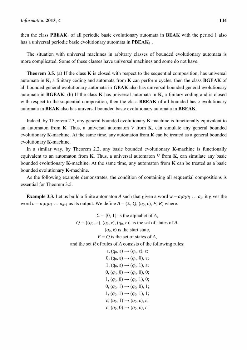
Example 3.3. Let us build a finite automaton A such that given a word w = a1a2a3 … an, it gives the
word u = a1a2a3 … an−1 as its output. We define A = (Σ, Q, (q0, ε), F, R) where:
Σ = {0, 1} is the alphabet of A,
Q = {(q0 , ε), (q0, ε), (q0, ε)} is the set of states of A,
(q0, ε) is the start state,
F = Q is the set of states of A,
and the set R of rules of A consists of the following rules:
ε, (q0, ε) → (q0, ε), ε;
0, (q0, ε) → (q0, 0), ε;
1, (q0, ε) → (q0, 1), ε;
0, (q0, 0) → (q0, 0), 0;
1, (q0, 0) → (q0, 1), 0;
0, (q0, 1) → (q0, 0), 1;
1, (q0, 1) → (q0, 1), 1;
ε, (q0, 1) → (q0, ε), ε;
ε, (q0, 0) → (q0, ε), ε;
Information 2013, 4 145
The expression a, (q0, b) → (q0, d), c means that given an input a and being in the state (q0, b), the
automaton A given c as its transition output and its outcome and make the transition to the state (q0, d).
A is a deterministic automaton. By definition, it is universal in the class KA = {A} that consists only
of the automaton A.
Let us consider bounded basic evolutionary KA-machines. They all have the form E = {A[t];
t = 1, 2, 3, ..., n} where all A[t] are copies of the automaton A. Such an evolutionary KA-machine E
works in the following way. Receiving a word w = a1a2a3 … an as its input, the automaton A[1]
produces the word u = a1a2a3 … an−1 as its transition output and the empty word ε as its outcome. Then
when n > 2, the automaton A[2] receives the word u = a1a2a3…an−1 as its input and produces the word
v = a1a2a3…an−2 as its transition output and the empty word ε as its outcome. This process continues
until the automaton A[n] receives the word a1 as its input. Then A[n] does not produce the transition
output (it is the empty word ε), while its outcome is equal to the word a1.
Any evolutionary machine in the class BBEAKA of all bounded basic evolutionary KA-machines
has the form E = {A[t]; t = 1, 2, 3, ..., n} where all A[t] are copies of the automaton A. However, such a
machine cannot be universal in the class BBEAKA because it cannot simulate the machine En+1 = {A[t];
t = 1, 2, 3, ..., n, n + 1} where all A[t] are copies of the automaton A. Indeed, on the input word
r = a1a2a3…anan+1 and on any longer input word, the machine E gives the empty outcome, while the
machine E gives the outcome a1 on the input word r. It means that the class BBEAKA does not have
universal automata although KA has universal automata.
4. Evolutionary Information Size
Here we introduce and study evolutionary information necessary to develop a constructive object by
a given system of evolutionary algorithms (evolutionary automata/machines). It is called evolutionary
or genetic information about an object or the evolutionary information size of an object. Here we
consider symbolic representation of objects. Namely, it is assumed that all automata/machines work
with strings of symbols (words) and all objects are such strings of symbols (words).
Let us consider a class H of evolutionary automata/machines. Note that that the initial population
X[0] is coded as one word in the alphabet of evolutionary automata/machines from H and its is
possible to consider this input as a representation p of the genetic information used to produce the
output population (object) x that satisfies the search condition. Evolutionary automata/machines from
H represent the environment in which evolution goes.
Definition 4.1. The quantity EISA(x) of evolutionary information about an object/word x, also called
the evolutionary information size EISA(x) of an object/word x with respect to an automaton/machine A
from H is defined as
EISA(x) = min {l(p); A(p) = x}
where l(p) is the length of the word p, while in the case when there are no words p such that
A(p, y) = x, EISA(x) is not defined.
Informally, the quantity of evolutionary information about an object x with respect to an automaton
A shows how much information it is necessary for building (computing or constructing) this object by
Information 2013, 4 146
means of the automaton A. Thus, it is natural that different automata need different quantity of
evolutionary information about an object x to build (compute or construct) this object.
However, people, computers and social organizations use systems (classes) of automata/algorithms
and not a single automaton/algorithm. To define the quantity of information about an object x with
respect to a class of automata/algorithms, algorithmic information theory suggests taking universal
automata/algorithms as representatives of the considered class. Such choice is grounded because it is
proved that so defined quantity of information about an object is additively invariant with respect to
the choice of the universal automaton/algorithm and is also additively optimal [5,8]. Similar approach
works in the case of evolutionary information.
Taking a universal automaton U in the class H, we can define relatively invariant optimal
evolutionary information about an object in the class H.
Definition 4.2. The quantity of evolutionary information about an object/word x, also called the evolutionary information size, EIS
H(x) of an object/word x with respect to the class H is defined as
EISH
(x) = min {l(p); U(p) = x}
while in the case when there are no words p such that U(p) = x, EISH
(x) is not defined.
Note that if there are no words p such that U(p) = x, then for any automaton A from H, there are no words p such that A(p) = x. In particular, the function EIS
H(x) is defined or undefined independently of
the choice of universal algorithms for its definition.
Informally, quantity of evolutionary information about an object x with respect to the class H shows
how much information it is necessary for building (computing or constructing) this object by means of
some automaton U universal in the class H.
Note that when H consists of a single automaton/machine A, functions EISH(x) and
EISA(x) coincide.
Example 4.1. Recursive evolutionary information size of (evolutionary information about) an object x is defined as EIS
H(x) when H is a class of evolutionary Turing machines.
Example 4.2. Inductive evolutionary information size of (evolutionary information about) an object x is defined as EIS
H(x) when H is a class of evolutionary inductive Turing machines.
It is possible to show that evolutionary information size (evolutionary information about an object
x) with respect to the class H is additively optimal when the automata from H have finite
simulation coding.
Theorem 4.1. If the class H has a finitary coding and the coding simulation <,> satisfies Condition
L, then for any evolutionary automaton/machine A from the class H and any universal evolutionary automaton U in H, there is a constant number cAU such that for any object/word x, we have
EISU(x) ≤ EISA(x; y) + cAU (1)
i.e., EISH(x) = EISU(x) is additively optimal.
Information 2013, 4 147
Proof. Let us take an evolutionary automaton/machine A from the class H and a word x. Then by
Definitions 3.1 and 4.1,
EISA(x) = min {l(q); A(q) = x} = l(q0)
and
EISU(x) = min {l(p); U(<c(A), p>) = x} = l(p0)
where <> is a coding of pairs of words. By Condition L, there is a number cv such that for any word
u from X*, we have
l(<c(A), p0>) ≤ l(p0) + cc(A)
Then as U(<c(A), p0>) = x, we have
EISU(x) = l(q0) ≤ l(<c(A), p0>) = l(p0) + cc(A)
Thus,
l(q0) ≤ l(p0) + cc(A)
and
EISU(x) ≤ EISA(x) + cAU
where cAU = cc(A). For the standard coding <,>, cc(A) = 2l(c(A)) + 1. It means that EISH(x) is additively
optimal.
Theorem is proved.
Inequality (1) defines the relation ≼ on functions, which is called the additive order [6–8], namely,
f(x) ≼ g(x) if there is a constant number c such that for any x, we have
f(x) ≤ g(x) + c (2)
Proposition 4.1. The relation ≼ is a partial preorder, i.e., it is reflexive and transitive.
Indeed, for any function f(x), we have f(x) ≤ f(x) + 0, i.e., the relation ≼ is reflexive.
Besides, if f(x) ≤ g(x) + c and g(x) ≤ h(x) + k, then we have f(x) ≤ h(x) + (c + k). It means that the
relation ≼ is transitive.
Thus, Theorem 4.1 means that information size with respect to a universal automaton/machine in H
is additively minimal in the class of information sizes with respect to automata/machines in H.
Theorems 3.3, 3.4, 4.1 and Proposition 3.3 imply the following result.
Corollary 4.1. If the class K has universal automata in K and a finitary simulation coding, then
evolutionary information size EISEU(x) with respect to a universal evolutionary automaton/machine EU
in the class PGEAK (PBEAK) of all periodic general (basic) evolutionary K-automata/K-machines is
additively minimal in the class of evolutionary information sizes with respect to evolutionary
K-automata/K-machines in PGEAK (PBEAK).
Information 2013, 4 148
The evolutionary information size EISPGEAK(x) with respect to the class PGEAK is defined as
evolutionary information size EISEU(x) with respect to with respect to some universal in PGEAK
evolutionary automaton/machine EU. The evolutionary information size EISPBEAK(x) with respect to the class PBEAK is defined as
evolutionary information size EISEU(x) with respect to with respect to some universal in PBEAK
evolutionary automaton/machine EU.
As the class of all Turing machines has universal Turing machines and a finitary simulation coding,
Corollary 4.1 implies the following result.
Corollary 4.2. There is an additively minimal evolutionary information size in the class of
evolutionary information sizes with respect to periodic general (basic) evolutionary Turing machines.
The evolutionary information size EISPGETM(x) with respect to the class PGETM of all periodic
general evolutionary Turing machines is defined as evolutionary information size EISEU(x) with
respect to with respect to some universal periodic general evolutionary Turing machine EU. The evolutionary information size EISPBETM(x) with respect to the class PBETM of all periodic
basic evolutionary Turing machines is defined as evolutionary information size EISEU(x) with respect
to with respect to some universal periodic basic evolutionary Turing machine EU.
As the class of all inductive Turing machines has universal inductive Turing machines and a finitary
simulation coding [7], Corollary 4.1 implies the following result.
Corollary 4.3. There is an additively minimal evolutionary information size in the class of
evolutionary information sizes with respect to periodic general (basic) evolutionary inductive
Turing machines.
The evolutionary information size EISPGEITM(x) with respect to the class PGEITM of all periodic
general evolutionary inductive Turing machines is defined as evolutionary information size EISEU(x)
with respect to with respect to some universal periodic general evolutionary inductive Turing
machine EU. The evolutionary information size EISPBEITM(x) with respect to the class PBEITM of all periodic
basic evolutionary inductive Turing machines is defined as evolutionary information size EISEU(x)
with respect to with respect to some universal periodic basic evolutionary inductive Turing
machine EU.
Theorem 4.1 and Proposition 3.3 imply the following result.
Corollary 4.4. If the class K has universal automata in K, is closed with respect to the sequential
composition and has a finitary simulation coding, then evolutionary information size with respect to a
universal evolutionary K-automaton/K-machine in the class BGEAK (BBEAK) of all bounded general
(basic) evolutionary K-automata/ K-machines is additively minimal in the class of evolutionary
information sizes with respect to evolutionary K-automata/K-machines in BGEAK (BBEAK).

Information 2013, 4 149
The evolutionary information size EISBGEAK(x) with respect to the class BGEAK is defined as
evolutionary information size EISEU(x) with respect to with respect to some universal evolutionary
automaton/machine EU the class BGEAK. The evolutionary information size EISBBEAK(x) with respect to the class BBEAK is defined as
evolutionary information size EISEU(x) with respect to with respect to some universal evolutionary
automaton/machine EU the class BBEAK.
As the class of all Turing machines has universal Turing machines, is closed with respect to the
sequential composition and has a finitary simulation coding, Corollary 4.4 implies the following result.
Corollary 4.5. There is an additively minimal evolutionary information size in the class of
evolutionary information sizes with respect to bounded general (basic) evolutionary Turing machines.
The evolutionary information size EISBGEITM(x) with respect to the class BGEITM of all bounded
general evolutionary inductive Turing machines is defined as evolutionary information size EISEU(x)
with respect to with respect to some universal bounded general evolutionary inductive Turing
machine EU. The evolutionary information size EISBBEITM(x) with respect to the class BBEITM of all bounded
basic evolutionary inductive Turing machines is defined as evolutionary information size EISEU(x)
with respect to with respect to some universal bounded basic evolutionary inductive Turing
machine EU.
As the class of all multitape inductive Turing machines has universal inductive Turing machines, is
closed with respect to the sequential composition (Theorem 2.3) and has a finitary simulation
coding [7], Corollary 4.4 implies the following result.
Corollary 4.6. There is an additively minimal evolutionary information size in the class of
evolutionary information sizes with respect to bounded general (basic) evolutionary multitape
inductive Turing machines.
There are specific relations between information sizes relative to different classes of
automata/algorithms.
Proposition 4.2. If Q ⊆ H, then EISH
(x) ≼ EISQ
(x).
As it is possible to consider any automaton from K as a bounded general or basic evolutionary
K-machine, Proposition 4.2 implies the following results.
Corollary 4.7. EISK
(x) ≼ EISBBETM(x) ≼ EISPBETM(x) ≼ EISAPBETM(x) ≼ EISAPBEITM(x) and
EISBBETM(x) ≼ EISBBEITM(x) ≼ EISPBEITM(x) ≼ EISAPBEITM(x).
Corollary 4.8. EISK
(x) ≼ EISBGETM(x) ≼ EISPGETM(x) ≼ EISAPGETM(x) ≼ EISAPGEITM(x) and
EISBGETM(x) ≼ EISBGEITM(x) ≼ EISPGEITM(x) ≼ EISAPGEITM(x).
Inequality ≼ defines the relation ≍ on functions, which is called the additive equivalence, namely,
f(x) ≍ g(x) if f(x) ≼ g(x) and g(x) ≼ f(x)
Information 2013, 4 150
Proposition 4.3. The relation ≍ is an equivalence relation.
Indeed, as the relation ≼ is reflexive and transitive, the relation ≍ is also reflexive and transitive. In
addition, by definition, the relation ≍ is symmetric, i.e., it is an equivalence relation.
Corollary 4.9. If the class H has a finitary coding, then for any two universal automata V and U in
H, there is a constant number kUV such that for any object/word x we have
EISU(x) ≤ EISV(x) + cUV
This shows that evolutionary information size (evolutionary information about an object x) with
respect to the class H is additively invariant when the automata from H have finite simulation coding.
Namely, we have the following result.
Theorem 4.2. If the class H has a finitary coding, then for any two universal automata V and U in
H, then evolutionary information sizes EISU(x) and EISV(x) are additively equivalent, i.e.,
EISU(x) ≍ EISV(x).
Proof. As V and U are both universal automata in H, by Theorem 4.1, for all words x, we have
EISU(x) ≤ EISV(x) + cUV
and
EISV(x) ≤ EISU(x) + cVU
Thus,
EISU(x; y) ≥ EISV(x; y) − cVy
It means that the quantities EIQU(y; x) and EIQV(y; x) of information in an object y are
additively equivalent.
Theorem is proved.
Definition 4.2 and properties of universal evolutionary algorithms imply the following result.
Proposition 4.4. If the class H has universal automata and an identity automaton, i.e., an automaton H such that H(x) = x for any word x in the language of the automata from H, then EISH(x) is a total
function on the set of all words the alphabet of the automata/machines from H.
Lemma 4.1. If the class K has an identity automaton, then all classes GEAK, BGEAK, PGEAK,
RGEAK, BEAK, BBEAK, PBEAK and RBEAK, have an identity automaton.
Lemma 4.1 and Proposition 4.4 show that evolutionary information size with respect to each of the
classes GEAK, BGEAK, PGEAK, RGEAK, BEAK, BBEAK, PBEAK and RBEAK is a
total function.
Corollary 4.10. Evolutionary information size EISBGETM(x) is a total function with respect to the
class BGETM of all bounded general evolutionary Turing machines is a total function.
Information 2013, 4 151
Corollary 4.11. Evolutionary information size EISBGEITM(x) is a total function with respect to the
class BGEITM of all bounded general evolutionary inductive Turing machines is a total function.
Corollary 4.12. Evolutionary information size EISPGETM(x) is a total function with respect to the
class PGEITM of all periodic general evolutionary Turing machines is a total function.
Corollary 4.13. Evolutionary information size EISPGEITM(x) is a total function with respect to the
class PGEITM of all periodic general evolutionary inductive Turing machines is a total function.
Corollary 4.14. Evolutionary information size EISBBETM(x) is a total function with respect to the
class BGETM of all bounded basic evolutionary Turing machines is a total function.
Corollary 4.15. Evolutionary information size EISBBEITM(x) is a total function with respect to the
class BGEITM of all bounded basic evolutionary inductive Turing machines is a total function.
Corollary 4.16. Evolutionary information size EISPBETM(x) is a total function with respect to the
class PGEITM of all periodic basic evolutionary Turing machines is a total function.
Corollary 4.17. Evolutionary information size EISPBEITM(x) is a total function with respect to the
class PGEITM of all periodic basic evolutionary inductive Turing machines is a total function.
Let us study other properties of the evolutionary information size.
Lemma 4.2. If A is a deterministic evolutionary automaton, then for any positive number n, there is
a positive number m such that inequality l(A(x)) > m implies inequality l(x) > n.
Proof. Let us take all words x1, x2, x3, …, xk with the length less than or equal to n. Then the lengths
of all words A(x1), A(x2), A(x3), …, A(xk) are bounded and we can define m = max {l(A(xi));
i = 1, 2, 3, …, k}. Taking a word w for which l(A(w)) > m, we see that w does not belong to the set
{x1, x2, x3, …, xk}. Thus, l(w) > n.
Lemma is proved.
Lemma 4.2 implies the following result.
Theorem 4.3. If a class H of evolutionary automata/machines has an identity automaton and
universal evolutionary automata/machines, while all automata from H are deterministic and have a
finitary coding, then EISH(x) → ∞ when l(x) → ∞.
Indeed, taking a universal evolutionary automaton/machine U from H, we see that by Lemma 4.2,
for any positive number n, there is a positive number m such that inequality l(A(x)) > m implies inequality l(x) > n. It means that if l(z) > m and EISH(z) = EISU(z) = r, then z = U(x) and EISU(z) = l(x).
Thus, inequality l(U(x)) > m implies inequality EISH(x) = EISU(x) > n. So, when l(x) → ∞, EISH(x)
also grows without limits.
Corollary 4.18. If all machines in TM are deterministic, then EISPGETM(x) → ∞ when l(x) → ∞.
Corollary 4.19. If all machines in ITM are deterministic, then EISPGEITM(x) → ∞ when l(x) → ∞.

Information 2013, 4 152
Corollary 4.20. If all machines in TM are deterministic, then EISPBETM(x) → ∞ when l(x) → ∞.
Corollary 4.21. If all machines in ITM are deterministic, then EISPBEITM(x) → ∞ when l(x) → ∞.
There are interesting relations between the length of a word and the evolutionary information size
of the same word.
Proposition 4.5. If the class H has universal automata and an identity automaton, i.e., an automaton
H such that H(x) = x for any word x in the language of the automata from H, then there is a number c
such that for any word x, we have
EISH(x) ≤ l(x) + c
Indeed, for an identity automaton H from H, we have
EISH(x) = l(x)
By Theorem 4.1, for all words x, we have
EISH
(x) ≤ EISH(x) + cH = l(x) + cH
and we can take c = cUH to get the necessary result.
Note that similar relations exist for other information sizes, such as recursive information size [6] or
inductive information size [7,8]. It is interesting to compare evolutionary information size EISPBETM(x) with respect to the class
PBETM of all periodic basic evolutionary Turing machines and information size EISTM(x) with
respect to the class TM of all Turing machines.
Theorem 4.4. For any increasing recursive function h(x) that tends to infinity when l(x) and
any inductively decidable set of finite objects (words) V, there are infinitely many elements x from V for which h(EISTM(x)) > EISPBETM(x).
Proof. As it is proved in [3], working in the inductive mode, evolutionary Turing machines can
simulate any simple inductive Turing machine computing the same word with the same input. As it is
demonstrated above a universal evolutionary Turing machine is periodic. Thus, for any object (word)
w, we have
EISPBETM(w) EISTM(w)
At the same time, by Theorem 18 from [19], For any increasing recursive function h(x) that tends to
infinity when l(x) → and any inductively decidable set V, there are infinitely many elements w from V for which h(EISTM(w)) > EISITM(w) where ITM is the class of all inductive Turing machines.
Consequently, we have
h(EISTM(x)) > EISPBETM(x)
Infinitely many elements x from V.
Theorem is proved.

Information 2013, 4 153
Theorem 4.4 means that evolution can essentially reduce information size of objects because for
infinitely many objects, their information size defined by periodic basic evolutionary Turing machines
is essentially less than their information size defined by Turing machines.
Corollary 4.22. In any recursive set V, there are infinitely many elements x for which ln2(EISTM(x)) > EISPBETM(x).
Corollary 4.23. For any natural number n and any recursive set V, there are infinitely many elements x for which (EISTM(x))1/n > EISPBETM(x).
5. Evolutionary Information in an Object
Here we introduce and study the quantity of evolutionary information in an object, e.g., in a text,
that allows making simpler development/construction of another object by a given system of
evolutionary algorithms (evolutionary automata).
To define evolutionary information in an object, we consider the set X* of all words in an alphabet
X and three mappings <,>: X* × X* → X*, λ: X* → X* and π: X* → X* such that for any words u and
v from X*, we have λ(<u, v>) = u and π(<u, v>) = v. The standard coding of pairs of words has the
following form
<u, v> = 1l(u)
0uv
where l(v) is the length of the word v. Its dual coding of pairs has the form
<u, v> = 1l(v)
0vu
To study relative information size and relative quantity of information, we need Condition L
introduced in Section 3 and its dual condition.
Condition L. For any word v from X*, there is a number cv such that for any word u from X*,
we have
l(<u, v>) ≤ l(u) + cv
For the coding of pairs dual to the standard coding <,>, the constant cv is equal to 2l(v) + 1.
As before, K is an arbitrary class of automata with input and two outputs, and H is an arbitrary class
of evolutionary automata/machines/algorithms. Taking automata from H, we can define the relative
quantity of evolutionary information about, or relative evolutionary information size of, an object
(word) x.
Definition 5.1. (a) The left quantity EISLA(x; y) of evolutionary information about an object/word x,
also called the left evolutionary information size EISLA(x; y) of an object/word x, with respect to an
automaton/machine/algorithm A from H relative to an object/word y is defined as
EISLA(x; y) = min {l(p); A(<p, y>) = x}
where l(p) is the length of the word p, while in the case when there are no words p such that
A(<p, y>) = x, EISLA(x; y) is not defined; (b) The right quantity EISR
A(x; y) of evolutionary information
about an object/word x, also called the right evolutionary information size EISRA(x; y) of an
Information 2013, 4 154
object/word x, with respect to an automaton/machine/algorithm A from H relative to an object/word y
is defined as
EISRA(x; y) = min {l(p); A(<y, p>) = x}
where l(p) is the length of the word p, while in the case when there are no words p such that
A(<p, y>) = x, EISRA(x; y) is not defined.
Informally, the relative quantity of evolutionary information about an object x relative to (with
respect to) an evolutionary automaton A shows how much information it is necessary for building
(computing or constructing) this object by means of the automaton A that has some additional
information y. For instance, some evolutionary automata, when they are given the object x, which
naturally contains all information about the construction (structure) of itself, do not need any additional
information to build (compute or construct) x. So, for these automata, the evolutionary information size
of relative to x is zero. At the same time, other evolutionary automata need a lot of additional
information to build (compute or construct) x even when the object x is given to them.
Proposition 5.1. If the class H has a finitary coding and the coding simulation <,> satisfies
Condition L, then for any evolutionary automaton/machine A from the class H, there is a constant number cAU such that for any object/word x, we have
EISA(x) ≤ EISRA(x; y) + cy
Proof. Let us take an evolutionary automaton/machine A from the class H and a word x. Then by
Definitions 3.1 and 4.1,
EISA(x) = min {l(q); A(q) = x} = l(q0)
and
EISRA(x; y) = min {l(p); U(<y, p>) = x} = l(p0)
By Condition L, there is a number cy such that for the word p0 from X*, we have
l(q0) ≤ l(<y, p0>) = l(p0) + cy
Thus,
EISA(x) ≤ EISRA(x; y) + cy
Proposition is proved.
Corollary 5.1. For any algorithm A from H, we have EISA(x) ≼ EISRA(x; y).
We can see that in a general case, the right relative evolutionary information size of an object x does
not coincide with the left relative evolutionary information size of an object x. This peculiarity shows
that the relative evolutionary information size depends not only on the additional information in the
word y but also how this word y is processed by the automaton A.
Definition 5.2. (a) The right quantity EISRA(x; y) of evolutionary information in an object/word y
about an object/word x with respect to an automaton/machine/algorithm A from H is defined as
Information 2013, 4 155
EIQRA(y; x) = EISR
A(x) − EISRA(x; y)
when both quantities are defined and EIQRA(y; x) is undefined otherwise; (b) The left quantity EISL
A(x; y)
of evolutionary information in an object/word y about an object/word x with respect to an
automaton/machine/algorithm A from H is defined as
EIQLA(y; x) = EISL
A(x) − EISLA(x; y)
when both quantities are defined and EIQLA(y; x) is undefined otherwise.
Informally, the quantity of evolutionary information in an object/word y about an object x with
respect to an automaton/machine/algorithm A shows to what extent utilization of information in y
reduces information necessary for building (computing or constructing) this object by means of the
automaton A without any additional information.
Here we encounter the problem of negative information because the quantity EIQLA(x; y) of
evolutionary information can be negative when the size EISLA(x; y) is larger than the size EISL
A(x).
This happens when, for example, the automaton A needs an additional program to extract the word y
from the code <y, p> given to it as the input for computing x.
In essence, there are three meanings of negative information:
(1) Information about something negative, i.e., information with a negative connotation, is called
negative information.
(2) Information expressed with a negation of something is called negative information.
(3) Information that has negative measure is called negative information.
Here we study evolutionary measures of information. Consequently, we are interested in the third
meaning. In the traditional approach to information, it is always assumed that the measure, e.g.,
quantity, of information is always positive. However, recently in their exploration of quantum
information, researchers came to the conclusion that there is quantum information with negative
measure [24,25].
The general theory of information also permits different types of information with negative
measures [8]. For instance, misinformation can be treated as a kind of negative information, or more
exactly, as information with the negative measure of correctness.
Evolutionary information theory, as well as algorithmic information theory, explains how
information can be negative. Indeed, information in a word (an object) y about a word (an object) x can
contain noise that makes computation (construction) of x more complicated. As a result, this
information will be negative.
Misleading information can also increase the information size of an object because it will demand
additional information for automata or algorithms to detect misleading, to eliminate it and to guide
automata or algorithms in the right direction. Thus, it becomes understandable that algorithmic
information in general and evolutionary information in particular can be negative in many situations.
Evolutionary information theory, as well as algorithmic information theory, also gives a grounded
solution to the information paradox called by Hintikka “scandal of deduction” [26]. Its essence is that
the traditional approach to information claims that deduction does give new information or new
knowledge, having no empirical content. For instance, if an agent knows p and q is deduced from p,
then it is assumed that the agent knows q.

Information 2013, 4 156
To understand the situation, we remind that deduction is an evolutionary process of and a tool for
evolutionary knowledge integration. Thus, it is natural to use evolutionary information theory for
making sense of the “scandal of deduction”.
According to this theory, extraction of information from a message (statement) is an evolutionary
process, while information content of the message (statement) depends not only on the message itself
but mostly on algorithms used for information extraction.
To illustrate this principle of evolutionary information theory, let us consider the following situation
that involved Mr. B and Mr. F.
Two men, Mr. B and Mr. F, are sitting at a train station not far from London. Little Mr. F feels
himself very important. He has read different articles and even some books about information. He even
wrote something in that area. So, he thinks he knows everything about information.
Eventually a third man comes and asks, “When does the train to London come?” Little Mr. F starts
thinking how to better share his wisdom advising that man to look into the schedule. But before Mr. F
is ready, Mr. B says: “The train to London either comes at 8 p.m. or does not come at 8 p.m.” Then he
gets up and leaves the station. The third man follows Mr. B.
Little Mr. F is shocked—why instead of telling something reasonable that passenger uttered a
sentence that was not informative at all. Indeed, according to MTI (Mathematical Theory of
Information), TWSI (Theory of Weakly Semantic Information) and TSSI (Theory of Strongly
Semantic Information) tautologies are not informative. Little Mr. F read this in the book “The
Philosophy of Information”.
May be, little Mr. F thinks, the goal of the response was mocking at the third man and now the third
man is going to punish that stupid passenger. Little Mr. F is happy with this thought.
However, the third man got some information from the tautological statement of Mr. B because
after leaving the station, the third man asks Mr. B, “Are you Mr. James Bond?” “Yes, I am,” answers
Mr. B. “Then”, says the third man, “let’s go to my car.”
This imaginary episode shows that information is a more complicated phenomenon than many think
and even tautologies can be informative depending on the context, a priory knowledge of the
communicating systems and on algorithms used for information extraction. The third man and Mr. F
applied different algorithms for understanding the answer of Mr. B and came to different results: due
to incorrect conjectures, Mr. F was not able to obtain any information, while the third man got
information he needed at that time.
As we did before, it is necessary to go from the quantity of evolutionary information with respect to
one algorithm to the quantity of evolutionary information with respect to systems of algorithms
because people, computers and social organizations use systems (classes) of automata/algorithms and
not a single automaton/algorithm. To define the quantity of information in an object y about an object x
with respect to a class of automata/algorithms, algorithmic information theory suggests using universal
automata/algorithms as representatives of the considered class [5,8]. Similar approach works in the
case of evolutionary information.
Taking a universal automaton U in the class H, we can define relatively invariant optimal
evolutionary information about an object in the class H.

Information 2013, 4 157
Definition 5.3. (a) The right quantity EISRH(x; y) of evolutionary information about an object/word
x, also called the evolutionary information size EISRH(x; y) of an object/word x, with respect to the
class H relative to an object/word y is defined as
EISRH(x; y) = min {l(p); U(<y, p>) = x}
in the case when there are no words p such that U(p, y) = x, EISH(x; y) is not defined; (b) The left
quantity EISLA(x; y) of evolutionary information about an object/word x, also called the left
evolutionary information size EISLA(x; y) of an object/word x, with respect to the class H relative to an
object/word y is defined as
EISLH(x; y) = min {l(p); U(<p, y>) = x}
in the case when there are no words p such that U(<p, y>) = x, EISLU(x; y) is not defined.
Examples of quantities of evolutionary information about an object x with respect to a class of
evolutionary automata/machines are recursive quantity of evolutionary information about an object x
in this case, e.g., H is one of the classes BGETM, PGETM, APGETM BGETM, PGETM or
APGETM) or inductive quantity of evolutionary information about an object x in this case, e.g., H is
one of the classes BGEITM, PGEITM, APGEITM BGEITM, PGEITM or APGEITM).
Note that if there are no words p such that U(p, y) = x, then for any evolutionary automaton A from
H, there are no words p such that A(p, y) = x. In particular, functions EISRH(x; y) and EISL
H(x; y) are
defined or undefined independently of the choice of universal algorithms for their definition.
Informally, quantity of evolutionary information about an object x with respect to the class H shows
how much information it is necessary for building (computing or constructing) this object by means of
some automaton U universal in the class H and having additional information y, i.e.,
EISH(x; y) = EISU(x; y).
Observe that when H consists of a single evolutionary automaton/machine A, the functions
EISH(y; x) and EISA(y; x) coincide.
It is possible to show that relative evolutionary information size (relative evolutionary information
about an object x) with respect to the class H is additively optimal when the automata from H have
finite simulation coding.
Theorem 5.1. If the class H has a finitary coding <,>, then for any evolutionary
automaton/machine A from the class H, any word y and any universal evolutionary automaton U in H, there is a constant number cAUy such that for any object/word x, we have
EISRU(x; y) ≤ EISR
A(x; y) + cAUy
when the coding <,> satisfies Condition L and universal algorithm U uses the direct pairing, while
EISLU(x; y) ≤ EISL
A(x; y) + cAUy
when the coding <,> satisfies Condition L° and universal algorithm U uses the dual pairing.
Proof. Let us assume that the coding <,> satisfies Condition L and take an evolutionary
automaton/machine A from the class H and a word x. Then by Definitions 3.1 and 4.1,

Information 2013, 4 158
EISRA(x; y) = min {l(q); A(<y, p>) = x} = l(q0)
and
EISRU(x; y) = min {l(p); U(<c(A), <y, p>>) = x} = l(p0)
where <,> is a coding of pairs of words and U uses the direct pairing. By Condition L, there are
numbers cy and cc(A) such that for any word u from X*, we have
l(<c(A), <p0 , y>>) ≤ l(<p0 , y>>) + cc(A) ≤ l(p0) + cy + cc(A) = l(p0) + cAUy
Then as U(<c(A), <p0, y>>) = x, we have
EISRU(x; y) = l(q0) ≤ l(<c(A), <p0 , y>>) ≤ l(p0) + c
AUy
Thus,
l(q0) ≤ l(p0) + cAUy
and
EISRU(x; y) ≤ EISR
A(x; y) + cAUy
For the standard coding <,>, cAUy = 2l(y) + 2l(c(A)) + 2. It means that EISL
H(x; y) is additively
optimal.
Proof of the second part is similar.
Theorem is proved.
There are various relations between relative and absolute evolutionary information sizes. For
instance, Proposition 5.1 implies the following result.
Corollary 5.2. EISH(x) ≼ EISRH(x; y).
As the class of all Turing machines satisfies all necessary conditions [20], Proposition 5.1 implies
the following results.
Corollary 5.3. (a) EISBGETM(x) ≼ EISRBGETM(x; y); (b) EISPGETM(x) ≼ EISR
PGETM(x; y);
(c) EISAPGETM(x) ≼ EISRAPGETM(x; y).
Corollary 5.4. (a) EISBBETM(x) ≼ EISRBBETM(x; y); (b) EISPBETM(x) ≼ EISR
PBETM(x; y);
(c) EISAPBETM(x) ≼ EISRAPBETM(x; y).
As the class of all inductive Turing machines satisfies all necessary conditions [20],
Proposition 5.1 implies the following results.
Corollary 5.5. (a) EISBGEITM(x) ≼ EISRBGEITM(x; y); (b) EISPGEITM(x) ≼ EISR
PGEITM(x; y);
(c) EISAPGEITM(x) ≼ EISRAPGEITM(x; y).
Corollary 5.6. (a) EISBBEITM(x) ≼ EISRBBEITM(x; y); (b) EISPBEITM(x) ≼ EISR
PBEITM(x);
(c) EISAPBEITM(x) ≼ EISRAPBEITM(x).
To compare left relative and absolute evolutionary information sizes, we use conditions introduced in [20].

Information 2013, 4 159
Weak Comparison Condition CPWv. Algorithms/automata from the class K allow one to
compute the following comparison predicate:
1,whenunde ined,when
i.e., for any words w and v, there is an algorithm/automaton Av in K that computes this predicate.
Right Weak Composition Comparison Condition RWCPAv. For any algorithm/automaton A in
K, the computing sequential composition A ° Av is a member of K.
Constant Condition CC. For any element v ∈ R*(K), the function gv , which always takes one and
the same value v, i.e., gv(u) = v for all u ∈ DD*(K), is computed by some algorithm/automaton Ev
from K.
Right Compositional Constant Condition RCCC. For any algorithm/automaton A from K, the computing sequential composition A ° Ev belongs to K.
Let us assume that the class K satisfies Conditions CPWv, RWCPAv , CC, and RCCC, while the
class H of evolutionary K-machines has a finitary coding and the coding <,> of pairs satisfies
Condition L, while the function λ: X* → X* is computed by some machine Cλ from K.
Proposition 5.2. For any evolutionary automaton/machine A from the class H and any universal evolutionary automaton U in H, there is a constant number cAU such that for any object/word x,
we have
EISLU(x; y) ≤ EISL
U(x) + cUy
Proof. Let us take, a universal automaton/machine V in the class K, a word y and build an
automaton/machine A from the class K such that gives the result x with an input <p, y> if and only if
V(p) = x. To do this, we define
A = Cλ ° V ° Ax ° Ex
By the listed properties of the class K, the automaton/machine A belongs to K.
Given the input <p, y>, the automaton/machine A works in the following way. At first, the
automaton/machine Cλ converts the word <p, y> into the word p. Then the universal
automaton/machine V works with p. When V does not give the result, A also does not give the result.
When V gives the result w, then w goes to the machine Ax as its input. If w is not equal to x, Ax does not
give the result. If w is equal to x, Ax gives the result 1. This result goes to the machine Ex as its input.
By properties of the machine Ex , its output is x. Thus, the automaton/machine A gives the result x with
an input <p, y> if and only if V(p) = x.
This allows us to build the evolutionary automaton/machine E = {A[t]; t = 1, 2, 3, ...} in which all
automata A[t] = A and the evolutionary automaton/machine U = {V[t]; t = 1, 2, 3, ...} in which all
automata V[t] = V (t = 1, 2, 3, ...). If H is the class of general evolutionary K-machines, then by
Theorem 3.1, U is a universal evolutionary automaton/machine in H. If H is the class of basic
evolutionary K-machines, then by Theorem 3.2, U is a universal evolutionary automaton/machine in
H. Thus,
EISLH
(x; y) = EISLU(x; y)

Information 2013, 4 160
By construction, the evolutionary K-machine E gives the result x with an input <p, y> if and only if U(p) = x. Consequently, EISL
A(x; y) = EISU(x) = EISH
(x).
By Theorem 5.1, for the evolutionary automaton/machine E, there is a constant number cEUy such
that for any object/word x, we have
EISLU(x; y) ≤ EISL
A(x; y) + cEUy
Consequently,
EISLU(x; y) ≤ EISU(x) + cEUy
Proposition is proved. As EISL
U(x; y) = EISLH
(x; y), we have the following result.
Corollary 5.7. EISLH
(x; y) ≼ EISH
(x).
As the class of all Turing machines satisfies all necessary conditions [20], Proposition 5.2 implies
the following results.
Corollary 5.8. (a) EISLBGETM(x; y) ≼ EISBGETM(x); (b) EISL
PGETM(x; y) ≼ EISPGETM(x);
(c) EISLAPGETM(x; y) ≼ EISAPGETM(x).
Corollary 5.9. (a) EISLBBETM(x; y) ≼ EISBBETM(x); (b) EISL
PBETM(x; y) ≼ EISPBETM(x);
(c) EISLAPBETM(x; y) ≼ EISAPBETM(x).
As the class of all inductive Turing machines satisfies all necessary conditions [20], Proposition 5.2
implies the following results.
Corollary 5.10. (a) EISLBGEITM(x; y) ≼ EISBGEITM(x); (b) EISL
PGEITM(x; y) ≼ EISPGEITM(x);
(c) EISLAPGEITM(x; y) ≼ EISAPGEITM(x).
Corollary 5.11. (a) EISLBBEITM(x; y) ≼ EISBBEITM(x); (b) EISL
PBEITM(x; y) ≼ EISPBEITM(x);
(c) EISLAPBEITM(x; y) ≼ EISAPBEITM(x).
Let us find what relations exist between right relative evolutionary information size and left relative
evolutionary information size of the same object. To do this, we consider the function sw: X* → X*
such that sw(<x, y>) = <y, x> for any elements x and y from X*.
Switching Code Condition SCC. The function sw is computed by some algorithm/automaton Asw
from K.
For instance, the code <u, v> = 1l(u)
0uv can be converted to the code <v, u> = 1l(v)
0vu by an
appropriate Turing machine.
Right Compositional Switching Code Condition RCSCCC. For any algorithm/automaton A from K, the computing sequential composition Asw ° A belongs to K.
Proposition 5.3. If the class H has a finitary coding, class K satisfies Conditions RCSCCC and
SCC, has free automata, while the coding simulation <,> satisfies Condition L, then for any word y
and for any universal evolutionary automaton/machine U from the class H, the right evolutionary
Information 2013, 4 161
information size EISRU(x) and the left evolutionary information size EISL
U(x) are additively equivalent,
i.e., EISRU(x) ≍ EISL
U(x).
Proof. Let us take, an evolutionary automaton/machine U = {U[t]; t = 1, 2, 3, ...} universal in the
class H in which all level automata U[t] are copies of a universal in K automaton V (cf. Theorem 3.1) and a word y. This allows us to build the evolutionary K-machine D = Asw ° U from the class H by
changing the first level automaton U[1] in U by the sequential composition Asw ° V. This sequential
composition exists in the K because K has free automata and satisfies Conditions RCSCCC and SCC.
Given the input <y, p>, the automaton/machine D works in the following way. At first, the
automaton/machine Asw converts the word <y, p> into the word <p, y>. Then the universal
automaton/machine U[1] = V works with <p, y>. Then the evolutionary process continues involving
machines U[t] with t = 2, 3, .... Thus, D(<y, p>) = U(<p, y>). Consequently,
EISRD(x; y) = EISL
U(x; y)
At the same time, by Theorem 5.1, for the evolutionary automaton/machine D, there is a constant number cDUy such that for any object/word x, we have
EISRU(x; y) ≤ EISR
D(x; y) + cDUy
Consequently,
EISRU(x; y) ≤ EISL
U(x; y) + cDUy
In a similar way, we prove
EISLU(x; y) ≤ EISR
U(x; y) + cGUy
for a constant number cGuy . Thus, we have
EISRU(x; y) ≍ EISL
U(x; y)
Proposition is proved. Optimality results allow us to define the quantities EISR
H(x; y) and EISLH(x; y) of evolutionary
information in an object/word y about an object/word x with respect to the class H.
Definition 5.4. (a) The right quantity EISRH(x; y) of evolutionary information in an object/word y
about an object/word x with respect to the class H is defined as
EIQRH(y; x) = EISR
U(x) − EISRU(x; y)
for some automaton U universal in the class H when both quantities are defined and EIQH(y; x) is
undefined otherwise; (b) The left quantity EISLA(x; y) of evolutionary information in an object/word y
about an object/word x with respect to the class H is defined as
EIQLH(y; x) = EISL
U(x) − EISLU(x; y)
for some automaton U universal in the class H when both quantities are defined and EIQH(y; x) is
undefined otherwise.
Informally, quantity of evolutionary information in an object/word y about an object x with respect
to the class H shows to what extent utilization of evolutionary information in y reduces evolutionary
Information 2013, 4 162
information necessary for building (computing or constructing) this object by means of some
evolutionary automaton U universal in the class H without any additional information. As EISL
U(x; y) = EISLH(x; y) and EISR
U(x; y) = EISRH(x; y), Proposition 5.3 implies the
following result.
Corollary 5.12. If the class H satisfies all necessary conditions from Proposition 5.3, EISR
H(x; y) ≍ EISLH(x; y).
Note that when the class H consists of a single evolutionary automaton/machine A, functions EIQH(y; x) and EIQA(y; x) coincide.
If the class H satisfies all necessary conditions from Proposition 5.2, then we have the
following results.
Corollary 5.13. EIQLH(x; y) ≽ 0.
As the class of all Turing machines satisfies all necessary conditions [20], Proposition 5.2 implies
the following results.
Corollary 5.14. (a) EIQLBGETM(x; y) ≽ 0; (b) EIQL
PGETM(x; y) ≽ 0; (c) EIQLAPGETM(x; y) ≽ 0.
Corollary 5.15. (a) EIQLBBETM(x; y) ≽ 0; (b) EIQL
PBETM(x; y) ≽ 0; (c) EIQLAPBETM(x; y) ≽ 0.
As the class of all inductive Turing machines satisfies all necessary conditions [20], Proposition 5.2
implies the following results.
Corollary 5.16. (a) EIQLBGEITM(x; y) ≽ 0; (b) EIQL
PGEITM(x; y) ≽ 0; (c) EIQLAPGEITM(x; y) ≽ 0.
Corollary 5.17. (a) EIQLBBEITM(x; y) ≽ 0; (b) EIQL
PBEITM(x; y) ≽ 0; (c) EIQLAPBEITM(x; y) ≽ 0.
It is possible to show that evolutionary information in an object y with respect to the class H is
additively invariant when the automata from H have finite simulation coding. Namely, we have the
following result.
Theorem 5.2. If the class H has a finitary coding, then for any two universal automata V and U in
H, the quantities EIQLU(y; x) and EIQL
V(y; x), as well as the quantities EIQRU(y; x) and EIQR
V(y; x) of
evolutionary information in an object y are additively equivalent.
Proof. Let us consider two universal automata V and U in H. Then
EIQLU(y; x) = EISU(x) – EISL
U(x; y)
and
EIQLV(y; x) = EISV(x) – EISL
V(x; y)
As V and U are both universal automata in H, by Theorem 4.1, we have
EISU(x) ≤ EISV(x) + cUV
Information 2013, 4 163
and by Theorem 5.1, we have
EISV(x; y) ≤ EISU(x; y) + cVy
Thus,
EISLU(x; y) ≥ EISL
V(x; y) − cVy
Consequently,
EIQLU(y; x) = EISU(x) – EISL
U(x; y) ≤ EISV(x) + cUV – (EISLV(x; y) − cVy)
= EISV(x) + cUV – EISLV(x; y) + cVy
= EISV(x) – EISLV(x; y) + (cUV + cVy )
= EIQLV(y; x) + c
where
c = cUV + cVy
In a similar way, we prove
EIQLV(y; x) ≤ EIQL
U(y; x) + k
Thus, the quantities EIQLU(y; x) and EIQL
V(y; x) of information in an object y are additively equivalent.
Proof for the quantities EIQRU(y; x) and EIQR
V(y; x) is similar.
Theorem is proved.
Theorem 5.2 shows additive invariance of the evolutionary information in an object y with respect
to the classes BGETM, PGETM, APGETM, BBEITM, PBEITM and APBEITM.
However, it is necessary to remark that evolutionary information is additively invariant only as a
function. For an individual object, choice of different universal algorithms for defining evolutionary
information can result in big differences in evolutionary information estimation for this object.
6. Modeling Physical Evolution with Evolutionary Machines
To demonstrate applicability of evolutionary information theory to all material processes, in this
section, we describe modeling physical evolution with evolutionary machines. In physics, evolution is
often called time evolution and is described as changes of the physical system states, which are brought
about by the passage of time and are subject to the corresponding physical laws. For instance, in the
Newtonian mechanics, time evolution of a collection of rigid bodies is portrayed by Newton’s laws of
motion. In Lagrangian mechanics, the laws of time evolution are represented by Lagrangian equations,
while in Hamiltonian mechanics, they are represented by Hamiltonian equations. The classical
quantum mechanics describes time evolution by the Schrödinger equation.
The standard interpretations and applications of evolutionary machines and computations include
optimization and modeling of biological and social processes [3,27,28]. However, evolutionary
machines allow other interesting and important interpretations and applications. One area of such
interpretations and applications concerns the very foundations of physics.
According to the basic physical theory called loop quantum gravity, geometry of space-time is
described by spin networks, while matter exists at the nodes of these spin networks [15–17]. In

Information 2013, 4 164
essence, a spin network is a labeled graph. In it, nodes represent volumes (or informally, “lumps” or
“bricks”) of space, which are basic spatial elements, and edges (called lines of spin networks) describe
boundaries (spatial surface areas) and connections of these spatial elements. Each node is marked by a
number and this number specifies the volume (quantity of space) represented by this node. In a similar
way, each line (link) is marked by a number and informally, this number specifies the area of the
surface represented by this line [16]. In a formal representation, a half integer number si is associated
with each link γi, or equivalently, an integer number pi, the “color”, marks this link and pi = 2si . In
such a way, a spin network is labeled (named) by numbers.
Every quantum state corresponds to a spin network. The mathematics that describes the quantum
states of spatial volumes and areas provides rules for how the nodes and lines (links) can be connected
and what numbers can be assigned to them. For instance, when a node has three links, then the labels
(colors) on the links satisfy the well-known Clebsh-Gordon condition: Each color is not larger than the
sum of the other two, and the sum of the three colors is even [17]. As a result, every spin network that
obeys the necessary rules corresponds to a quantum state.
Subatomic particles, such as quarks or electrons, correspond to certain types of nodes in a spin
network, and are represented by adding more labels on nodes [17]. These labels signify physical
characteristics of the corresponding particles. Physical fields, such as the electromagnetic field, are
represented by additional labels on lines in a spin network. These labels indicate physical
characteristics of the corresponding fields.
This shows that spin networks are special cases of named sets, namely they are labeled networks or
labeled graphs, while matter is represented in loop quantum gravity by naming (labeling)
operations [29].
Material particles change their positions and interact with one another and with physical fields,
while physical fields change their characteristics. These changes are naturally modeled by naming
operations, such as renaming and reinterpreting [15,29]. Moreover, according to general relativity, the
geometry of space also changes with time. The bends and curves of the physical space change as
matter and energy move, and waves can pass through it like ripples on a lake [30]. In loop quantum
gravity, these processes are modeled by operations with the spin networks [15], which can be
mathematically described by operations with named sets [29].
Interestingly, there are computational models that work with labeled networks or labeled graphs.
The first of such models is called a Kolmogorov algorithm [7,31]. In contrast to the most popular
algorithmic models, such as Turing machines or formal grammars, Kolmogorov algorithms work not
with words but with configurations. A configuration consists of groups of symbols connected by
relations, i.e., a configuration is a labeled graph, in which nodes are labeled (named) by groups of
symbols, while edges are labeled by names of relations. Hypertexts [32] give an example of
configurations in which nodes are labeled by texts. Other examples of configurations are discrete
labeled graphs. Naturally, a configuration can represent a spin network. Making Kolmogorov
algorithms work with spin networks allows them to describe dynamics of material particles and fields.
Evolutionary Kolmogorov algorithms, i.e., evolutionary K-machines where the class K consists of
Kolmogorov algorithms, can naturally model evolution of space time and matter.
One more type of models that represent dynamics in labeled networks is Petri nets and their
advanced version—colored Petri nets [33,34]. A Petri net A is a system (P, T, in, out) that consists of
Information 2013, 4 165
two sets—the set of places P and the set of transitions T—and two functions—the input function in
that defines directed arcs from places to transitions and output function out that defines directed arcs
from transitions to places. Places usually represent states or resources in the system, while transitions
model the activities of the system. In such a way, Petri nets provide an efficient and mathematically
rigorous modeling framework for discrete event concurrent dynamically systems. Interpreting Petri
nets as spin networks allows them to model dynamics of material particles and fields. Consequently,
evolutionary Petri nets, i.e., evolutionary K-machines where the class K consists of Petri nets, can
naturally depict evolution of space time and matter.
The third type of models that represent dynamics in labeled networks comprises Turing machines
with a structured memory, inductive Turing machines with a structured memory and limit Turing
machines with a structured memory [7]. Structured memory, which is a system of cells with a variety
of connections between them, provides flexible tools for representation of spin networks, while
machines that work with structured memory can reflect dynamics of spin networks, and thus, portray
dynamics of material particles and fields. Consequently, evolutionary Turing machines with a
structured memory, evolutionary inductive Turing machines with a structured memory and
evolutionary limit Turing machines with a structured memory can naturally model evolution of space
time and matter.
Note that Petri net modeling of spin network dynamics is different from the realization of these
processes by (evolutionary) Kolmogorov algorithms, (evolutionary) Turing machines with a structured
memory, (evolutionary) inductive Turing machines with a structured memory and (evolutionary) limit
Turing machines with a structured memory. While a computational machine or a Kolmogorov
algorithm has a unified system of rules for changing spin networks, Petri nets work guided by local
rules. These local rules represent local dynamics of spin networks. However, it is possible to show that
(evolutionary) Turing machines with a structured memory can model both (evolutionary) Petri nets and
(evolutionary) Kolmogorov algorithms [7], i.e., local rules can be represented by a system of context
dependent global rules. At the same time, the structured memory allows using local rules of
transformation, which depend on the processed area in the structured memory.
7. Conclusions
Using universal evolutionary machines/automata, we introduced and studied several measures of
evolutionary information, i.e., information used in evolutionary processes. These measures include
relative and absolute evolutionary information sizes and evolutionary information in one object about
another object. Conditions were found when these measures are optimal and invariant.
This brings us to the following problems:
Problem 1. Study relations between evolutionary information and quantum information.
Evolution is very important in biology, being directed by genetic processes. This gives us a natural
direction for evolutionary information theory application.
Problem 2. Study biological information in general and genetic information in particular from the
evolutionary information perspective.
Information 2013, 4 166
The role of social evolution in society makes principal the following problem.
Problem 3. Explore social processes by means of evolutionary information.
The general theory of information [8] provides a universal context for evolutionary information
theory, supplying necessary tools and structures for efficient research. Thus, it would be interesting to
examine the following directions.
Problem 4. Study evolutionary processes in spaces of information operators.
Spaces of information operators are built and studied based on functional analysis. Another
mathematical model for the general theory of information utilizes category theory. Thus, we have a
similar problem in the context of algebraic categories.
Problem 5. Study evolutionary processes in categories of information operators.
Evolutionary computations in general and genetic algorithms in particular are efficient tools for
optimization [27,28].
Problem 6. Study complexity of optimization problems using evolutionary information theory.
Evolutionary automata are utilized for modeling and exploration of collaboration processes [35].
Problem 7. Apply evolutionary information theory to find how collaboration can decrease complexity
in solving various problems.
In this paper, the main concern was evolutionary information for classes of evolutionary
automata/algorithms that have universal automata/algorithms.
Problem 8. Study properties of evolutionary information for classes of evolutionary automata/algorithms
that do not have universal automata/algorithms.
Evolutionary computations have been used simulation of communication and language
evolution [36,37]. Thus, it would be natural to find information characteristics of these processes.
Problem 9. Study communication and language evolution using evolutionary information theory.
It is possible to put this problem in a more general context.
Problem 10. Study cultural evolution using evolutionary information theory.
References
1. Garzon, M.H. Evolutionary computation and the processes of life: On the role of evolutionary
models in computing. In Proceeding of Ubiquity Symposium, November 2012.
2. Burgin, M.; Eberbach, E. Universality for Turing machines, inductive Turing machines and
evolutionary algorithms. Fundam. Inform. 2009, 91, 53–77.
Information 2013, 4 167
3. Burgin, M.; Eberbach, E. On foundations of evolutionary computation: An evolutionary automata
approach. In Handbook of Research on Artificial Immune Systems and Natural Computing:
Applying Complex Adaptive Technologies; Mo, H., Ed.; IGI Global: Hershey, PA, USA, 2009;
pp. 342–360.
4. Burgin, M.; Eberbach, E. Bounded and periodic evolutionary machines. In Proceeding of 2010
Congress on Evolutionary Computation (CEC′2010), Barcelona, Spain, 2010; pp. 1379–1386.
5. Chaitin, G.J. Algorithmic Information Theory; Cambridge University Press: Cambridge, UK, 1987.
6. Li, M.; Vitanyi, P. An Introduction to Kolmogorov Complexity and its Applications;
Springer-Verlag: New York, NY, USA, 1997.
7. Burgin, M. Superrecursive Algorithms; Springer: New York, NY, USA, 2005.
8. Burgin, M. Theory of Information: Fundamentality, Diversity and Unification; World Scientific
Publishing: Singapore, 2010.
9. Dodig-Crnkovic, G. Significance of models of computation from Turing model to natural
computation. Minds Mach. 2011, 21, 301–322.
10. Dodig-Crnkovic, G.; Müller, V. A dialogue concerning two world systems: Info-computational vs.
mechanistic. In Information and Computation; Dodig-Crnkovic, G., Burgin, M., Eds.; World
Scientific: Singapore, 2011; pp. 149–184.
11. Fredkin, E. Digital mechanics. Physica D 1990, 45, 254–270.
12. Lloyd, S. A theory of quantum gravity based on quantum computation. Available online:
http://arxiv.org/abs/quant-ph/0501135 (accessed on 12 March 2013).
13. Wolfram, S.A. New Kind of Science; Wolfram Media: Champaign, IL, USA, 2002.
14. Zuse, K. Rechnender Raum; Friedrich Vieweg & Sohn: Braunschweig, Germany, 1969.
15. Smolin, L. Three Roads to Quantum Gravity; Basic Books: New York, NY, USA, 2001.
16. Smolin, L. Atoms of space and time. Sci. Am. 2004, 15, 66–75.
17. Rovelli, C. Quantum Gravity; Cambridge University Press: Cambridge, UK, 2004.
18. Burgin, M. Multiple computations and Kolmogorov complexity for such processes. Not. Acad. Sci.
USSR 1983, 27, 793–797.
19. Burgin, M. Algorithmic complexity of recursive and inductive algorithms. Theor. Comput. Sci.
2004, 317, 31–60.
20. Burgin, M. Measuring Power of Algorithms, Computer Programs, and Information Automata;
Nova Science Publishers: New York, NY, USA, 2010.
21. Burks, A.; Wright, J. The theory of logical nets. Proc. Inst. Radio Eng. 1953, 41, 1357–1365.
22. Blum, L.; Cucker, F.; Shub, M.; Smale, S. Complexity and Real Computation; Springer-Verlag:
New York, NY, USA, 1997.
23. Burgin, M. Universal limit Turing machines. Not. Rus. Acad. Sci. 1992, 325, 654–658.
24. Wright, B.D. Negative information. Rasch Meas. Trans. 1996, 10, 504.
25. Horodecki, M.; Oppenheim, J.; Winter, A. Partial quantum information. Nature 2005, 436, 673–676.
26. Hintikka, J. Logic, Language Games and Information; Clarendon: Oxford, UK, 1973.
27. Michalewicz, Z. Genetic Algorithms + Data Structures = Evolution Programs; Springer-Verlag:
New York, NY, USA, 1996.
28. Michalewicz, Z.; Fogel, D.B. How to Solve It: Modern Heuristics, 2nd ed.; Springer-Verlag:
New York, NY, USA, 2004.
Information 2013, 4 168
29. Burgin, M. Theory of Named Sets; Nova Science Publisher: New York, NY, USA, 2011.
30. Gibbs, W.W. Ripples in spacetime. Sci. Am. 2002, 286, 62–71.
31. Kolmogorov, A.N. On the concept of algorithm. Rus. Math. Surv. 1953, 8, 175–176.
32. Nielsen, J. Hypertext and Hypermedia; Academic Press: New York, NY, USA, 1990.
33. Peterson, J.L. Petri Net Theory and the Modeling of Systems; Prentice-Hall, Inc.: Englewood Cliffs,
NJ, USA, 1981.
34. Petri, C. Kommunikation mit Automaten. Ph.D. Thesis, University of Bonn, Bonn, Germany, 1962.
35. Burgin, M.; Eberbach, E. Cooperative combinatorial optimization: Evolutionary computation case
study. BioSystems 2008, 91, 34–50.
36. Christiansen, M.H.; Kirby, S. Language evolution: Consensus and controversies. Trends Cogn.
Sci. 2003, 7, 300–307.
37. Nowak, M.A.; Krakauer, D.C. The evolution of language. Proc. Natl. Acad. Sci. USA 1999, 96,
8028–8033.
© 2013 by the authors; licensee MDPI, Basel, Switzerland. This article is an open access article
distributed under the terms and conditions of the Creative Commons Attribution license
(http://creativecommons.org/licenses/by/3.0/).