Evolutionary Portfolio Selection

with Liquidity Shocks

Enrico De Giorgi∗

Institute for Empirical Economic ResearchUniversity of Zurich

First Draft: 17th December 2003

This Version: 27th April 2004

Abstract

Insurance companies invest their wealth in financial markets. The wealth evolutionstrongly depends on the success of their investment strategies, but also on liquidityshocks which occur during unfavourable years, when indemnities to be paid to theclients exceed collected premia. An investment strategy that does not take liquidityshocks into account, exposes insurance companies to the risk of bankruptcy, whenliquidity shocks and low investment payoffs jointly appear. Therefore, regulatory au-thorities impose solvency restrictions to ensure that insurance companies are able toface their obligations with high probability. This paper analyses the behaviour of in-surance companies in an evolutionary framework. We show that an insurance companythat merely satisfies regulatory constraints will eventually vanish from the market. Wegive a more restrictive no bankruptcy condition for the investment strategies and wecharacterize trading strategies that are evolutionary stable, i.e. able to drive out anymutation.

Keywords: insurance, portfolio theory, evolutionary finance.

JEL Classification Numbers: G11, G22, D81.

SSRN Classification: Capital Markets: Asset Pricing and Valuation, Banking and Finan-cial Institutions.

∗I am grateful to Thorsten Hens and Klaus Schenk-Hoppe for their valuable suggestions. Financialsupports from Credit Suisse Group, UBS AG and Swiss Re through RiskLab, Switzerland and from thenational center of competence in research “Financial Valuation and Risk Management” and are gratefullyacknowledged. The national centers of competence in research are managed by the Swiss National ScienceFoundation on behalf of the federal authorities.

1 Introduction

Institutional investors, like pension plans or insurance companies, are usually active on assetmarkets that do not provide complete insurance against all possible risks. The performance ofthose institutions strongly depends on the success of their investment strategies. On the otherhand, pension plans and insurance companies are also exposed to liquidity shocks, that occurwhen the pensions or claims to be paid out to the clients exceed collected premia. In orderto ensure that insurance companies or pension plans are able to face their obligations withhigh probability, regulatory authorities impose solvency constraints, that are constraints onthe investment strategies, such that a safely invested reserve capital exists. A part from theregulatory constraints, institutional investors still face the problem of choosing the proportionof wealth to be invested prudently, in order to be able to cover future losses and, therefore,to avoid going bankrupt, but, on the other hand, to also profit from growth opportunitiesoffered by financial markets.

In this paper we analyse the long-run performance of insurance companies with an evo-lutionary model, that is well suited to study the performance of large institutional investors,since they have a considerable impact on asset prices, face relatively small transaction costsand their investment horizon is potentially infinite.According to this approach, investors’ trading strategies compete for the market capitaland the endogenous price process is thus a market selection mechanism along which somestrategies gain market capital while others lose. Analogously, insurance companies sell in-surance contracts depending on their ability of facing liquidity shocks, and premia are alsoendogenously determined by demand and supply. We use the theory of dynamical systems(Arnold 1998) to derive evolutionary stable trading stable strategies, i.e. those that havethe highest exponential growth rate in a population where they determine asset prices.

The evolutionary model that we present in this paper, has one long-lived risky asset andcash. Withdrawals and savings are the difference between collected premia and pensions orindemnities to be paid. Here, in particular, we consider insurance companies, and the pricingprinciple for insurance contracts is given by regulatory constraints, set up to ensure that withtheir supply for insurance contracts, insurance companies are able to face their obligationswith high probability. This relates to the investment strategies, i.e. the proportion of wealthsafely invested, so that, finally, regulatory constraints represent minimal requirements oninvestors’ investment strategies. A bankruptcy occurs when the investment’s payoff and pre-mia are not enough to pay the indemnities. Moreover, borrowing and short-selling are notallowed, so investors that go to bankrupt simply disappear from the market. We establish ano bankruptcy condition for the investment strategies. The no bankruptcy condition is theminimal sufficient condition on the trading strategies that ensures that, in the presence ofany type of competitor or trading strategy, the investor is able to face almost surely liquidityshocks. In fact, since asset prices are endogenously determined, it happens that, dependingon other players’ strategies and wealth shares, with any strategy that satisfies a less restric-tive condition than the no bankruptcy condition, the probability of going bankrupt is strictly

1

positive. In particular, if an investor is the unique survivor at some point in time, the nobankruptcy condition is sufficient but also necessary to avoid almost surely going bankrupt.Nevertheless, while investors with strategies satisfying the no bankruptcy condition will notalmost surely go bankrupt, we also show that investors who use the simple strategy thatcorresponds to the no bankruptcy boundary, will eventually disappear from the market.Moreover, we characterize trading strategies that are evolutionary stable, if they exist, fol-lowing the idea first introduced by Hens and Schenk-Hoppe (2002a). We give the conditionon the dividend process and liquidity shocks factor for the existence of evolutionary stablestrategies, when the state of the world follows an i.i.d. process. We show that the conditionfor the existence of evolutionary stable strategies is related to the growth rate of the trad-ing strategies in a neighbourhood of the strategy investing according to the no bankruptcyboundary. If this growth rate is strictly positive, then an investor putting more than the nobankruptcy boundary on the risky assets is able to further increase her market share, whenasset prices are dominated by the strategy corresponding to the no bankruptcy boundary.However, this is true only as long as liquidity shocks do not force the investor to use all herwealth, or else she will disappear from the market. Therefore, while it can happen that thegrowth rate of a strategy in a neighbourhood above the no bankruptcy boundary is positive,this strategy cannot be evolutionary stable, since it will almost surely disappear, because ofliquidity shocks. In this case, no evolutionary stable strategies could exist. This result alsosuggest that in the presence of liquidity shocks, evolutionary stability should be character-ized in term of both the growth rate and the probability of default.

This work contributes to the development of the evolutionary portfolio theory, that startedwith the seminal paper of Blume and Easley (1992), where an asset market model is firstintroduced to study the market selection mechanism and the long run evolution of investors’wealth and assets’ prices. In their model, Blume and Easley (1992) consider diagonal se-curities1, with no transaction costs and positive proportional saving rates are exogenouslygiven. In the case of complete markets with diagonal securities, Blume and Easley (1992)show that there is a unique attractor of the market selection mechanism and prices do notmatter. With simple strategies2 and constant, identical saving rates across investors, theunique survivor is the portfolio rule known as “betting your beliefs” (Breiman 1961), wherethe proportion of wealth to be put on each asset is the probability of the corresponding stateof nature. This strategy can also be generated by maximizing the expected logarithm ofrelative returns, which is know as the Kelly rule, studied in discrete-time by Kelly (1956),Breiman (1961), Thorp (1971) and Hakansson and Ziemba (1995) (for an overview, seealso Ziemba 2002) and, in continuous-time, by Pestien and Sudderth (1985), Heath, Orey,Pestien, and Sudderth (1987) and Karatzas and Shreve (1998), among others. Hens and

1A system of securities is called diagonal, if for each state of nature there is exactly one asset which hasa strictly positive payoff.

2A portfolio rule called a simple strategy, if the proportion of wealth put on each asset is constant overtime.

2

Schenk-Hoppe (2002a) proposed a more general setting, with incomplete markets, generalshort-lived assets that re-born each period and constant, positive, proportional and, identicalsaving rates across investors. In their evolutionary model, the equilibrium notion refers towealth distributions that are invariant under the market selection process. The authors showthat invariant wealth distributions are generated by a population, where only one investor(or portfolio rule) exists (a so-called monomorphic population). Moreover, they introducethe concept of evolutionary stable portfolio rules, that is also considered in this paper. Themain result of Hens and Schenk-Hoppe (2002a) is that, in the case of ergodic state of theworld processes and without redundant assets, there is a unique evolutionary stable portfoliorule, which is the one that puts on each asset the proportion of wealth corresponding to theexpected relative payoff of the asset. In Evstigineev, Hens, and Schenk-Hoppe (2003) thisresult is extended to a model with long-lived assets, under the assumption of Markow stateof the world. Introducing long-lived assets allows to take into account the capital gains andlosses due to assets’ prices changes. This will also be of much importance in the presenceof liquidity shocks, as we will discuss in this paper. Moreover, in Evstigneev, Hens, andSchenk-Hoppe (2002) it is also shown that, with independent and identically distributedstate of world processes, the strategy that invests according to relative dividends is theunique simple portfolio rule that asymptotically gathers total wealth. A generalization ofthe results obtained by Blume and Easley (1992). Sandroni (2000), and Blume and Easley(2002) have also studied the case of long-lived assets, to include market prices in the evolu-tion of wealth shares. The main result of Blume and Easley (2002) and Sandroni (2000), isthat, with complete markets, among all infinite horizon expected utility maximizers, thosewho happen to have rational expectation will eventually dominate the market and this resultholds independently of investors’ risk aversion. In his model Sandroni (2000) also includesendogenously determined positive and proportional saving rates.All these models assume that withdrawals and savings are a positive proportion of the cur-rent wealth, so that bankruptcy is excluded in their setup. Moreover, e.g. in Evstigineev,Hens, and Schenk-Hoppe (2003), the withdrawal rates are assumed to be identical amonginvestors. Under these assumptions, the only criterion that matters for a trading strategy tobe evolutionary stable, is its exponential growth rate in the presence of a mutant strategy.This paper shows that with non-proportional and maybe negative withdrawal rates, a secondcriterion has to be considered, since in fact, even if a strategy has the maximal exponentialgrowth rate in the presence of any mutant, it can disappear because exogenously determinedliquidity shock occurs.

In the classical finance approach with exogenously given price dynamics, asset-liabilitymanagement models already assume that investors maximize the investment’s expected pay-off less penalties for bankruptcy or targets not meet (see Carino, Myers, and Ziemba 1998,Carino and Ziemba 1998). Liu, Longstaff, and Pan (2003) consider a price dynamic for therisky asset with jumps (event risk) and take utility functions identical to −∞ for strictlynegative terminal wealth, so that no portfolio rule, that has a strictly positive probability

3

of going bankrupt, will be optimal. They obtain lower (since they do not exclude short-selling) and upper bounds for the proportion of wealth to be put on the risky asset and theyprovide optimal portfolio weights. Alternatively, Browne (1997) distinguishes between thesurvival problem and the growth problem. He first looks at portfolio rules that maximizethe probability of surviving in the so-called danger-zone (where bankruptcy has strictly pos-itive probability to occur) and second, he considers portfolio rules that maximize the growthrate in the safe-zone, where bankruptcy is almost surely excluded. Browne (1997) identifieswealth-level dependent strategies, but in his time-continuous setup, no optimal strategy isfound for the danger-zone, and a weaker optimality criterion is introduced. The optimalstrategy for the safe-zone corresponds to a generalization of the Kelly criterion previouslydiscussed. Zhao and Ziemba (2000) propose a model with a reward function on minimumsubsistence, i.e. the objective function to maximize equals the sum of the expected finalwealth and a concave increasing function on the supremum over the wealth levels that arealmost surely smaller than final wealth. In this way, the optimal portfolio rule solves atrade-off between expected payoff and minimum subsistence.

The rest of this paper is organized as follows. In the next section we present the modelsetup. In Section 3 we derive the no bankruptcy condition on investment strategies, thatensures that liquidity shocks do not cause bankruptcy. In Section 4 we present the mainresults of the paper. Section 5 concludes. Technical results and proofs are given in theAppendix.

2 An evolutionary model with bankruptcy

Time is discrete and denoted by t = 0, 1, 2, . . . . Uncertainty is modelled by a stochasticprocess (St)t∈Z with values in some infinite space S, endowed with power σ-algebra 2|S|.F t = σ(. . . , S0, S1, . . . , St) denotes the σ-algebra giving all the information available at timet and F = σ (∪t∈ZF

t). Let Ω = SZ be the space of sample paths (st)t∈Z, where st, t ∈ Z

is the realization of St on S. Finally, P denotes the unique probability measure on (Ω,F)generated by (St)t∈Z. There are i = 1, . . . , I (I ≥ 2) investors, with initial wealth wi

0.There is one long-lived risky asset and cash. Cash is risk-less both in terms of its return

R = 1 + r ≥ 1 and price, which is taken as numeraire. The risky asset pays a dividendDt(s

t) ≥ 0 at time t, depending on the history st = (. . . , s−1, s0, s1, . . . , st) up to timet. Moreover, at each time t each investor i withdraws or collects the amount Ci

t(st), also

depending on the history st up to time t. Here, we consider insurance companies, so that Cit

is the difference between the indemnities to be paid and collected premia.Let wi

t be the total wealth of investor i at time t after claims’ payment and premia collection,mi

t ≥ 0 and ait ≥ 0 be the unit of cash and risky asset, respectively, held by investor i at

time t and qt be the price of the risky asset. The budget constraint at time t of each investor

4

i is given bywi

t = mit + qt a

it. (1)

The wealth of investor i evolves as follows3

wit+1 = (1 + r) mi

t + (Dt+1 + qt+1) ait − Ci

t+1. (2)

We say that investor i goes bankrupt during period (t, t + 1] (or simply period t + 1) iffwi

t+1 ≤ 0. In this case she uses all her wealth to pay the indemnities and vanishes fromthe market, i.e. we arbitrarily write mi

s = ais = 0 for all s ≥ t + 1 (and thus we also set

wis = 0 for all s ≥ t + 1). Note that the investor’s wealth at time t + 1 also depends on the

price qt+1 of the risky asset, which is determined at equilibrium by investors’ demand for therisky asset and supply. Thus, time t + 1 investors’ strategies may cause a bankruptcy. LetIt = i |wi

t > 0 be the set of investors, who survive period t. Obviously, It ⊆ It−1 and thusmi

t = ait = 0 for all i 6∈ It−1. Investor j is said to be the unique survivor at time t if and

only if It = j.The next period amount Ci

t+1 is determined by the following. At time t investor i candecide to sell δi

t ≥ 0 insurance contracts on one single future stochastic claim Xt+1 ≥ 0(which is identical for all investors). The premium Pt+1 of each contract is F t-measurable(depends only on information available up to time t), determined by the market clearingcondition on the insurance market at time t, and is paid at time t + 1 by the buyer of theinsurance contract, who is supposed to be external to the economy just defined, i.e. buyersof insurance contracts do not participate to the financial market. The amount collected orwithdrawn by investor i at time t + 1 is then given by the difference

Cit+1 = δi

t (Xt+1 − Pt+1)

between claims and premia.We suppose that the insurance market is regulated and solvency constraints are imposed.Each investor i should be able to meet her obligation, in a way that conditioning on thecurrent history st only a proportion αi

t > 0 of her current wealth will be affected with asmall probability ǫi

t > 0, i.e.

P[δit (Xt+1 − Pt+1) > αi

t wit |s

t]

= ǫit (3)

where for all t and i ∈ It

αit ∈ (0, α) and ǫi

t ≤ ǫ. (4)

3To be formally correct, the wealth evolution of equation (2) should be replaced by

wi

t+1 =[(1 + r)mi

t+ (Dt+1 + qt+1) ai

t− Ci

t+1

]+,

where for x ∈ R, x+ = max(0, x). We prefer to keep the notation simpler and since we are essentiallylooking at strategies that survive in the long run, the wealth evolution of those strategies is correctly givenby equation (2).

5

The parameters α and ǫ are exogenously given by regulatory authorities. Equation (3)defines the pricing rule for insurance contracts and is called quintile principle and it hasbeen discussed in Schnieper (1993) and Embrechts (1996). Moreover, it corresponds tothe proportional value-at-risk constraints studied by Leippold, Vanini, and Trojani (2003)with time independent proportional factors, and sameness between investors in their generalequilibrium consideration. The parameters αi

t and ǫit are fixed and can be interpreted as the

“loss acceptability” of investor i and, in the general setting of the model, we assume thatthey can vary between investors. Other simplifying assumptions will be introduced later. Fora given premium Pt+1 and parameters αi

t and ǫit, equation (3) serves to compute the number

δit of insurance contracts that investor i can sell, in order to satisfy the solvency constraint.

The premium Pt+1 is determined endogenously when the insurance market clears.We should bear in mind that for an investor, going bankrupt means vanishing from

the market and thus should be avoided! They can further decrease their insurance risk bychoosing a smaller αi or a smaller ǫi. As we will see below, an investor with a small αi, whois a “safer investor” with respect to minimal solvency requirement, is also forced to reduceher exposure to the insurance market, “losing” in this way growth opportunities when claimsare less than premia. The amount αi

t wit represents the technical reserve or the proportion of

current wealth to be invested prudently by investor i to make the risky insurance businessacceptable in the future (see Norberg and Sundt 1985). If the amount δi

t (Xt+1 − Pt+1) isstrictly greater than the technical reserves, we say that investor i faces a liquidity shock .From equation (3), investor i faces liquidity shocks with probability ǫi

t during period t + 1.

In our setting, the solvency constraint essentially imposes that mit ≥

αit

Rwi

t, for all i, orequivalently

mit

wit

≥αi

t

R, ∀i ∈ It. (5)

Let µt = E[Xt |F

t−1]

and σ2t = Var(Xt |F

t−1) be the conditional expectation and the con-ditional variance of Xt, given F t, respectively, and let Ft be the conditional cumulativedistribution function of Yt = Xt−µt

σt, i.e.

Ft(y) = P[Yt ≤ y |F t−1

].

Moreover, F−1t denotes the generalized inverse of Ft. To avoid the premium Pt+1 fully

covering the insurance risk, we impose the following restrictions

Assumption 1 (Insurance market). For t ∈ Z and i ∈ It, let (αit, ǫ

it) and (αi

t, ǫit) be two

possible choices for the loss acceptability parameters of investor i. Let αit = αi

t. Then for allpremia Pt+1

δit > δi

t ⇒ ǫit > ǫi

t.

This assumption says that for given technical reserves, the probability of having liquidityshocks strictly increases with the number of insurance contracts sold. If this is not satisfied,

6

then it would be possible to cover additional insurance risk only through collected premia,which is not a fair pricing rule. Since δi

t = 0 solves equation (3) with αit = 0 and ǫi

t = 0,Assumption 1 also implies that an insurance company without technical reserves that sells astrictly positive number of contracts, faces liquidity shocks with a strictly positive probability.Assumption 1 indirectly imposes restrictions on equilibrium premia, as shown in the followinglemma.

Lemma 1. If Assumption 1 holds, then for all t ∈ Z and i ∈ It:

Pt+1 < µt+1 + σt+1 F−1t+1(1 − ǫi

t).

Proof. Let us suppose that

Pt+1 ≥ µt+1 + σt+1 F−1t+1(1 − ǫi

t).

for some t and i ∈ It. ThenPt+1 − µt+1

σt+1

≥ F−1t+1(1 − ǫi

t)

and thus for all δ > 0

P[δ (Xt+1 − Pt+1) > 0

]= P

[Xt+1 − Pt+1 > 0

]= P

[Yt+1 >

Pt+1 − µt+1

σt+1

]≤ ǫi

t

independently from δ. This contradicts Assumption 1, since the last inequality shows thatthe probability of liquidity shocks is in fact independent of the number of contracts, withfixed technical reserves.

From equation (3) and Lemma 1, we obtain

δit

[µt+1 + σt+1 F−1

t+1(1 − ǫit) − Pt+1

]= αi

t wit, (6)

or

δit =

αit w

it

µt+1 + σt+1 F−1t+1(1 − ǫi

t) − Pt+1

. (7)

Lemma 1 ensures that δit ≥ 0. Equation (7) says that investor i supply for insurance con-

tracts is proportional to her technical reserve and decreases with increasing probability ǫit.

For a fixed supply of insurance contracts, an investor can therefore decrease her technicalreserve by decreasing her liquidity shock probability ǫi

t. Naturally, the solvency constraints(3) and (4) do not take into account the magnitude of a liquidity shock! This is a well knowcritique of quintile constraints (see e.g. Artzner, Delbaen, Eber, and Heath 1997).

We assume that demand for insurance contracts is normalized to 1, i.e.∑

i δit = 1 for all

t. It follows:Pt+1 = µt+1 + σt+1

∑

i

δit F−1

t+1(1 − ǫit) −

∑

i

αit w

it. (8)

7

σt+1

∑

i δit F−1

t+1(1− ǫit)−

∑

i αit w

it is the so-called loading factor and is supposed to be strictly

positive. In fact, it is well known from the ruin theory, that if Pt+1 ≤ µt+1, i.e. if thepremium at time t is less or equal to the conditional expectation of next period claims givenall information available at time t, then for any value for the initial wealth (without financialmarket) the probability of going bankrupt is equal one (see Feller 1971, page 396). Fromthe last equation, we see that the premium of the insurance contract increases with in-creasing conditional variance, as one would expect, and decreases when the weighted wealth∑I

i=1 αit w

it increases. Moreover, a safer investor, with a smaller αi or a smaller ǫi than a

riskier investor, contributes to an increase of the premium, from which all investors benefit.This behaviour has also been described by Ceccarelli (2002). Equations (7) and (8) can besolved for δi

t and Pt+1: they provide a unique solution with a strictly positive premium (thiswill become clear for the special case considered below; however, we give a general proof ofthe existence and uniqueness of a solution in the Appendix 6.1).

Since the goal of this paper is to analyse investors’ long-run wealth evolution with respectto their investment strategies on financial markets, we assume that their profiles on insurancemarkets are identical, meaning that they possess the same loss acceptability parameters.Here, we do not address the question of investors’ strategies (choice of the loss acceptabilityparameters) on the insurance market. It is not clear whether an investor who has higherloss acceptability, will growth faster or not. In fact, while it is true by equation (7) thathigher loss acceptability means greater liquidity shocks (for both the probability and theamount), it must also be said that investors who sell a larger number of contracts benefitfrom growth opportunities when premia are greater than claims. Moreover, less technicalreserves means a smaller exposure to liquidity shocks (as discussed above), but also lessrestrictive constraints for the investment strategies, meaning that those investors can putless money into the risk-free asset and profit from growth opportunities on the financialmarket. We address these issues in other works. Here, as in Leippold, Vanini, and Trojani(2003) we make the following assumption.

Assumption 2 (Loss acceptability).Investors’ “loss acceptability” is constant over time and identical for all investors, i.e. αi

t =α ∈ (0, α) and ǫi

t = ǫ for all t and i = 1, . . . , I.

Note that by equations (7) and (8), when all investors possess the same ǫit, δi

t does not dependon ǫi

t anymore and therefore the magnitude of liquidity shocks is minimized for all investorsif ǫi

t = ǫ. Moreover, by Assumption 2 and equations (7) and (8) it follows

Pt+1 = µt+1 + σt+1 F−1t+1(1 − ǫ) − α

∑

i

wit, (9)

δit =

wit

∑

j wjt

, (10)

8

and therefore investor’s i supply for insurance contracts corresponds to her relative wealth.

Now, we introduce a precise structure for the claim Xt+1. In particular, we assume thatthe total claim Xt+1 is proportional to the aggregate wealth available at time t, meaningthat the amount of insured claims increases or decreases depending on the aggregate successof the investors (a similar assumption will be also made for the dividend process). Thisassumption also prevents a shock from destroying the economy. The proportional factor issupposed to be independent of the history up to time t and can be interpreted as the liquidityshock factor for the economy. Mathematically we have

Xt+1 = ηt+1 Wt, (11)

where ηt+1 ∈ [0, 1] is independent of F t and Wt =∑

i∈Itwi

t =∑I

i=1 wit is the aggregate wealth

available in the economy at time t. From equation (11) it follows that µt+1 = Wt E[ηt+1

]

and σ2t+1 = W 2

t Var(ηt+1). Moreover, ηt+1 ∼ Gt+1 where Ft+1(y) = Gt+1(y

Wt), ∀y. Thus

Pt+1 =(µ(ηt+1) + σ(ηt+1) G−1

t+1(1 − ǫ) − α)

Wt.

Therefore, the premium Pt+1 is strictly positive for all t, if the loading factor (σ(ηt+1) G−1t+1(1−

ǫ) − α) Wt is greater than zero for all t. Moreover, for the sake of simplicity, we make thefollowing assumption:

Assumption 3 (Liquidity shocks).Liquidity shocks (ηt)t≥1 are independent and identically distributed, i.e. Gt = G for all t,ηt ∼ η ∼ G, where G is a continuous cumulative distribution function.

Let µ = E[η]

and σ2 = Var(η), then by Assumptions 2 and 3,

Pt+1 = µWt + σ G−1(1 − ǫ) Wt − α Wt = (β − α) Wt, (12)

Cit+1 = (ηt+1 − β + α) wi

t, (13)

where β = µ + σ G−1(1 − ǫ). As discussed above for the general case, we impose that theloading factor (σ G−1(1 − ǫ) − α) Wt is strictly positive, i.e. α < minα, σ G−1(1−ǫ). Thenβ − α > β − σ G−1(1 − ǫ) = µ > 0 and thus Pt+1 > 0 for all t.

We now turn our attention to the financial market. We suppose that the risky assetis in fixed supply, normalized to one. Instead, the supply of cash is exogenously given bycumulated dividends and collected premia less withdrawals. The market clearing conditionsare

I∑

i=1

ait =

∑

i∈It

ait = 1 (14)

Mt = R∑

i∈It

mit−1 + Dt

∑

i∈It

ait−1 − qt

(

1 −∑

i∈It

ait−1

)

− Cit (15)

9

where Mt =∑

i∈Itmi

t and Ct =∑

i∈ItCi

t . Note that∑

i∈Itmi

t−1 ≤ Mt−1 =∑

i∈It−1mi

t−1

since It ⊆ It−1. Moreover, if no bankruptcy occurs during period t, then It = It−1 and theusual equation for Mt follows, i.e. Mt = R Mt−1 + Dt − Ct. Note that Mt ≥ 0 for all t. Infact if for some t, Mt < 0, then there exists at least one investor, say j ∈ It, with mj

t < 0.But since borrowing is not allowed, investor j is forced into bankruptcy during period t, acontradiction to j ∈ It.To be consistent with Assumption 3, and in order to avoid that dividends become very smallas compared to insurance shocks, we make the following assumption for the dividend process:

Assumption 4 (Dividend process).

(i) For each t,Dt = dt Wt−1,

for some process (dt)t>0, with dt ∼ d ∼ H independently and identically distributedwith cumulative distribution function H on [0, 1].

(ii)P[d > 0

]= 1 − H(0) ∈ (0, 1),

i.e. at each time dividends have strictly positive probability of being zero and of beingstrictly positive.

This assumption, together with Assumption 3, solves the difficulty encountered by Hensand Schenk-Hoppe (2002b), where the rate of return on the long-lived asset eventually dom-inates that of the numeraire, so that the strategy that invests only in long-lived asset is ableto drive out any other strategy. Hens and Schenk-Hoppe (2002b) suggest to base evolution-ary finance model on Lucas (1978), where assets’ payoffs are in term of a single perishableconsumption good. In this way, the consumption rate is at least as the growth rate of thetotal payoff of the market. In our model, also without relaying on Lucas (1978), the pricingrule for insurance contracts (that also determines Ct) and, Assumption 3 and 4, ensure thatthe rate of “consumption” increases proportionally to the growth rate of the total payoff.Moreover, as will discuss later, if assets’ payoffs were in term of perishable consumptiongoods, it would not be possible to find a trading strategy that preserves the wealth (thereserve capital in the insurance business) and have positive growth rate.

Let λit ∈ [0, 1] be the proportion of wealth invested in the risky asset by investor i ∈ It

at time t. We have

ait =

λit w

it

qt

and mit = (1 − λi

t) wit.

We call the sequence (λit)t>0 | i∈It the trading strategy of investor i and λi

t the strategy ofinvestor i at time t. We use the convention that λi

t = 0 if i /∈ It. Note that λit is a random

variable, i.e. it depends on the state of the world up to time t, st. Other assumptions on the

10

process defining the trading strategy (λit)t≥0 will be introduced later. Here, we just impose

the following restriction on the strategies at time t, (λit)i∈It

, to prevent the price of the riskyasset from becoming zero.

Assumption 5 (Investors’ strategies).For each t such that |It| > 1, there exists i, j ∈ It with (1 − λi

t) λjt > 0.

Assumption 5 essentially states that if more than one investor survives period t, then thereexists at least one survivor with a strictly positive proportion of her wealth invested inthe risky asset and one survivor with a strictly positive proportion of her wealth investedin the risk-free asset. Naturally, when a survivor has a mixed strategy4 λi

t ∈ (0, 1), thenAssumption 5 is obviously satisfied with i = j. If |It| = 1, then it might occur that theunique survivor uses a strategy investing all her wealth in the risk-free asset. The strategyλi

t = 1 is excluded by the solvency constraint. In fact, the solvency condition stated byequation (5) is equivalent to

1 − λit ≥

α

R⇔ λi

t ≤ 1 −α

R=: λ ∈ (0, 1), (16)

i.e., for each investor, the proportion of wealth invested in the risky asset is bounded fromabove by λ. It seems to be a natural restriction for an insurance company (or a pensionfund), as shown e.g. in Davis (2001, Tables 5 and 6) for life insurances and pension fundsof several countries. Let λt = (λ1

t , . . . , λIt )

′, then the market clearing condition for the riskyasset (14) implies

qt = λ′twt.

Note that for i /∈ It, wit = 0 by assumption and thus λ′

twt =∑

i∈Itλi

t wit. We rewrite

equation (2) as follows

wit+1 =

[

R (1 − λit) + (dt+1 Wt + qt+1)

λit

qt

− (ηt+1 − β + α)

]

wit. (17)

3 The no bankruptcy condition

Before discussing the long run wealth evolution of investment strategies, we give conditionsfor avoiding bankruptcy. In fact, a necessary condition for long-term survival is not to gobankrupt and strategies that do not almost surely exclude bankruptcy are avoided by in-vestors with long-term horizon. Therefore, as in Browne (1997) and Liu, Longstaff, and Pan(2003), we distinguish between the conditions on the strategies to avoid going bankrupt and

4A strategy (λi

t)t is called a mixed strategy, iff it assigns a strictly positive percentage to every asset, for

all t. In our setting, a mixed strategy is characterized by λi

t∈ (0, 1) for all t (see Evstigneev, Hens, and

Schenk-Hoppe 2002).

11

then, given that investors satisfy those conditions, we analyses the long-term wealth evolu-tion. In our setting, analogously to Liu, Longstaff, and Pan (2003), we obtain upper boundsfor the λi

t’s (a lower bound is given by the no short sale restriction). We will show belowthat an investor with a strategy that does not prevent bankruptcy at each period, has astrictly positive probability of vanishing from the market, even if she is the unique survivor.Moreover, if an investor uses a simple strategy that does not prevent bankruptcy, she hasprobability 1 of vanishing from the market, even if at some point in time she is the uniquesurvivor and thus dominates assets’ prices. In particular, an investor holding only the riskyasset (i.e. λi

t = 1) becomes extinct with probability 1. This result shows that Theorem 1 inHens and Schenk-Hoppe (2002b) does not hold when bankruptcy can occur.

We first consider the case |It| = 1 for some t > 0, i.e. It = j for some j ∈ 1, . . . , I.We restrict ourself to strategies λj

t > 0. If λjt = 0, as is clearly excluded since R >

sup supp(η) − β + α5! The price of the risky asset at time t is given by qt = λjt wj

t andthe aggregate wealth at time t is Wt = wj

t : from equation (17) it follows immediately that

j ∈ It+1 ⇔ R (1 − λjt) − (ηt+1 − β + α) + dt+1 > 0.

Let η = inf supp(η), η = sup supp(η) and d = sup supp(d) and K be the continuous

multivariate cumulative distribution of (η, d) on [η, η] × [0, d], i.e.

K(x, y) = P[η ≤ x, d ≤ y

].

Moreover, let K(z) = P[d − η ≤ z

]=

∫ η

η

∫ x+z

0dK(x, y) be the cumulative distribution

function of d − η. Then

P[j ∈ It+1

]= P

[dt+1 − ηt+1 > −R (1 − λj

t) − β + α]

= 1 − K(−R (1 − λjt) − β + α)

and thus

P[j ∈ It+1

]= 1 ⇔ λj

t ≤R + k + β − α

R=: λ, (18)

where k = inf supp(K). We call this latter equation the no bankruptcy condition. Note that

λ = λ +β + k

R.

Therefore, the solvency constraint (16) is a stronger condition on the strategies than theno bankruptcy condition (18), if β > −k, i.e. if higher shocks (greater than β) on the

5supp(η) denotes the support of η.

12

insurance market and small dividends (less the η − β) in the financial market do not occursimultaneously, which is not a realistic assumption. This is due to the fact that the solvencyconstraint does not care about dividends, and thus does not take into consideration the(positive) correlation between shocks and dividends, such that higher shocks will have asmaller impact on the wealth evolution since they correspond to higher dividends. If β < −k(which is the most common case, as for example when insurance shocks and dividends areconsidered independent), the no bankruptcy condition (18) is stronger than the solvencyconstraint and thus investors just care about the no bankruptcy condition (18). In thiscase, the solvency constraint (16) does not eliminate bankruptcy! In the sequel we make thefollowing assumption on the joint distribution of (η, d):

Assumption 6 (Shocks and dividends joint distribution).For all δ1 > 0 and δ2 > 0,

P[η > η − δ1, d ≤ δ2

]> 0,

i.e., big shocks and very small dividends have strictly positive probability to jointly occur.

Assumption 6 implies the following Lemma on the distribution of d − η.

Lemma 2. For all δ > 0,P[d − η ≤ −η + δ

]> 0

and thus k = −η, i.e. maximal shocks and zero dividends have strictly positive probability tojointly occur.

Proof.

P[d − η ≤ −η + δ

]= P

[d ≤ η − η + δ

]

=

∫

0<δ1<δ

P[d ≤ η − η + δ |η − η > −δ1

]d P

[η − η > −δ1

]

≥

∫

0<δ1<δ

P[d ≤ −δ1 + δ |η − η > −δ1

]d P

[η − η > −δ1

]

=

∫

0<δ1<δ

P[d ≤ −δ1 + δ, η > η − δ1

]

P[η > η − δ1

]

︸ ︷︷ ︸

>0

d P[η − η > −δ1

]

> 0

Thus, K(−η + δ) > 0 for all δ > 0, i.e. k = −η.

Under Assumption 6, the strategy λ corresponds to R−η+β−α

Rand is a stronger condition on

the strategies than the solvency constraint, since obviously β < −η. From now on, we take

λ =R − η + β − α

R.

13

Let us now consider a single survivor j with a simple strategy λj > λ. Then at each periodshe will have a strictly positive probability of going bankrupt and therefore P

[j ∈ ∩tIt

]= 0,

meaning that she will vanish almost surely from the market. We state these results in thefollowing Lemma.

Lemma 3. Let It = j for some t and j ∈ 1, . . . , I, i.e. investor j is the unique survivorat time t. The following holds:

(i) If λjt > λ, then investor j has strictly positive probability of going bankrupt during

period t + 1.

(ii) If λjs > λ for all s ≥ t, then investor j will almost surely eventually vanish from

the market. In particular, if investor j uses a simple strategy λj > λ, then she willeventually almost surely vanish from the market almost surely.

Let us now consider the case |It| > 1. Without loss of generality we set It = 1, 2:if It = i1, . . . , in with n = |It| > 2, then we can still reduce the original setting to a2-investors setting by defining a “new investor” with strategy ξs ∈ [0, 1] at time s ∈ t, t+1and wealth ws, where

ξs =

∑n

l=2 λils wil

s∑n

l=2 wils

, ws =n∑

l=2

wils .

The price of the risky asset at time s ∈ t, t + 1 is then given by qs = λi1s wi1

t + ξs ws. Thuslet us assume that It = 1, 2. Then from the wealth evolution (17) it follows immediatelythat for i = 1, 2

i ∈ It+1 ⇔ R (1 − λit) + dt+1 Wt

λit

qt

+ wjt+1 λj

t+1

λit

qt

− (ηt+1 − β + α) > 0, (19)

where j 6= i.

Proof. (i) Suppose that i ∈ It+1. Then wit+1 > 0 and by equation (17)

wit+1 = R (1 − λi

t) wit + dt+1 Wt

λit w

it

qt

+

+(w1

t+1 λ1t+1 + w2

t+1 λ2t+1

) λit w

it

qt

− (ηt+1 − β + α) wit,

and thus

wit+1

(

1 − λit+1

λit w

it

qt

)

= R (1 − λit) wi

t + dt+1 Wt

λit w

it

qt

+wjt+1 λj

t+1

λit w

it

qt

− (ηt+1 − β + α) wit,

14

where j 6= i. Since λit+1 6= 1 (solvency restriction), then

(

1 − λit+1

λit wi

t

qt

)

> 0, and thus

from wit+1 > 0 it follows that

R (1 − λit) wi

t + dt+1 Wt

λit w

it

qt

+ wjt+1 λj

t+1

λit w

it

qt

− (ηt+1 − β + α) wit > 0.

Since i ∈ It, then wit > 0 and therefore dividing the last inequality by wi

t we obtain

R (1 − λit) + dt+1 Wt

λit

qt

+ wjt+1 λj

t+1

λit

qt

− (ηt+1 − β + α) > 0.

(ii) Suppose now that

R (1 − λit) + dt+1 Wt

λit

qt

+ wjt+1 λj

t+1

λit

qt

− (ηt+1 − β + α) > 0,

where j 6= i. Then for i ∈ It,

wit

[

R (1 − λit) + dt+1 Wt

λit

qt

+ wjt+1 λj

t+1

λit

qt

− (ηt+1 − β + α)

]

> 0,

and thus wit+1 > 0, since

wit+1 =

wit

R (1 − λit) + dt+1 Wt

λit

qt+ wj

t+1 λjt+1

λit

qt− (ηt+1 − β + α)

1 − λit+1

λit wi

t

qt

+

and 1 − λit+1

λit wi

t

qt> 0 by equation (16).

The necessary and sufficient condition (19) for avoiding bankruptcy for investor i also

depends on other investors’ wealths and strategies, through the term wjt+1 λj

t+1λi

t

wit

. Spec-

ulating on other investors’ behaviour, investor i could essentially put less wealth on therisk-free asset than allowed under the no bankruptcy condition (18). While this would implya strictly positive probability of going bankrupt when investor i dominates assets’ prices,the no bankruptcy condition is not necessary for avoiding almost surely bankruptcy in thepresence of competitors, when they significantly invest in the risky asset. However, the nobankruptcy condition is the minimal condition on investment strategies that almost surelyeliminates bankruptcy in the presence of each type of competitor. In fact, an investor whosystematically violates the no bankruptcy condition (18), will eventually disappear from themarket with probability one, if her opponents are investing all their wealth on the risk-freeasset, i.e. an investment strategy that systematically violates the no bankruptcy condition

15

is almost surely driven out by the risk-free strategy. Thus the no bankruptcy conditionis the minimal condition that ensures that each investor will not go bankrupt with prob-ability 1, regardless from other investors’ behaviour. In the sequel, because of the longhorizon perspective considered here, and following the approach of Liu, Longstaff, and Pan(2003), we use the no bankruptcy condition to ensure that investors almost surely do notface bankruptcy. In their setting, bankruptcy is penalized with minus infinity utility, so thatno optimal strategy will allow final negative wealth with strictly positive probability.

4 The main results

From the previous section, it is clear that an investor who uses a strategy that does notalmost surely eliminate bankruptcy, will eventually disappear from the market, also if atsome point in time she is the unique survivor. Thus, looking at the long-run evolutionof investors’ wealths, a strategy that does not prevent bankruptcy would not be fit, as it isdefined in Blume and Easley (1992). Neither can’t be evolutionary stable, as defined in Hensand Schenk-Hoppe (2002a) and Evstigineev, Hens, and Schenk-Hoppe (2003), since it willalso disappear almost surely if it dominates asset prices, as shown in Lemma 3. Moreover,as long as dividends and liquidity shocks are not positive correlated, the solvency restrictionis not enough to avoid bankruptcy. In fact, under the solvency restriction, an investor facesliquidity shocks with strictly positive probability and if her investment strategy providessmall payoff (in particular, dividends are small), then the liquidity shock destroys her wealth.Following the discussion of the previous section, we consider the case where the followingassumption holds and we study the long run evolution of investors, who are safe enough ontheir investment positions to be almost surely able to face liquidity shocks.

Assumption 7 (The no bankruptcy condition).For all i ∈ It and all t ∈ Z,

λit ∈ [0, λ].

Following Hens and Schenk-Hoppe (2002b), we rewrite the wealth dynamics. We define

Bit =

λit w

it

λ′t wt

,

and

Ait = R (1 − λi

t) wit + Bi

t dt+1 Wt − (ηt+1 − β + α) wit.

By Assumption 7, we have

wt+1 = At + Bt λ′t+1 wt+1

16

or

(I − Bt λ′t+1)wt+1 = At

where At = (A1t , . . . , A

It )

′, Bt = (B1t , . . . , B

It )

′ and I is the identity on RI . Note that for

i /∈ It, Ait = Bi

t = 0. The inverse of I − Bt λ′t+1 is given by I + (1 − λ′

t+1 Bt )−1 Bt λ′t+1,

provided that λ′t+1 Bt 6= 1 (see Horn and Johnson 1985, Sec. 0.7.4). It can be easily checked

that λ′t+1 Bt < 1 if there exits an investor i ∈ It+1 with λi

t < 1 and λit+1 > 0 and this is still

the case when |It| > 1, by Assumptions 5 and 7. If It = j for some j, then investor j isalready the unique survivor and the wealth evolution is easily obtained. Therefore, in thesequel we only consider the case |It| > 1. Under the assumption of no default during periodt + 1, the wealth evolution can then be written as

wt+1 =(I − Bt λ

′t+1

)−1At

=

(

I +Btλ

′t+1

1 − λ′t+1Bt

)

At, (20)

and the i-th component is given by

wit+1 =

wit

∑

j(1 − λjt+1) λj

t wjt

×

×

[

dt+1 Wt λit +

[R(λ − λi

t) + (η − ηt+1)]

(

λ′twt +

∑

j 6=i

(λit − λj

t)λjt+1 wj

t

)]

.

This result is explicitly derived in the Appendix 6.2. We use that

λ =R − η + β − α

R⇐⇒ R + β − α = R λ + η.

The price at time t + 1 follows:

qt+1 = λ′t+1 At +

λ′t+1 Bt λ

′t+1 At

1 − λ′t+1 Bt

=λ′

t+1 At

1 − λ′t+1 Bt

.

Let rit =

wit

Wt, and ζ i

t =λi

t

λfor i = 1, . . . , I and t ∈ Z. The vector rt = (r1

t , . . . , rIt )

′ is the

vector of wealth shares, i.e. rt ∈ ∆I−1 = r ∈ Ri+ |

∑

i rit = 1. By Assumption 7, ζ i

t ∈ [0, 1]and ζ i

t = 1 iff λit = λ. We obtain

wit+1 =

rit Wt

∑

j(1 − λ ζjt+1) ζj

t rjt

×

×

[

dt+1 ζ it +

[R λ (1 − ζ i

t) + (η − ηt+1)]

(

ζ ′trt + λ

∑

j 6=i

(ζ it − ζj

t ) ζjt+1 rj

t

)]

.

17

Let θt+1 be defined by

θt+1 = ζ ′trt dt+1 +

+∑

k

(

R λ (1 − ζkt ) + (η − ηt+1)

)

rkt

(

ζ ′trt + λ

∑

j

(ζkt − ζj

t ) ζjt+1 rj

t

)

.

Then

Wt+1 =θt+1

∑

j(1 − λ ζjt+1) ζj

t rjt

Wt.

The ratio θt+1∑

j(1−λ ζjt+1

) ζjt r

jt

is the growth rate of the economy. From the wealth evolution of

equation (20), we obtain the evolution of wealth shares:

rit+1 =

rit

θt+1

×

×

[

dt+1ζit +

[R λ (1 − ζ i

t) + (η − ηt+1)]

(

ζ ′trt + λ

∑

j

(ζ it − ζj

t )ζjt+1r

jt

)]

.

(21)

From this last equation it follows directly that rit+1 = 0 if ri

t = 0 and therefore also, rit+1 = 1

if rit = 1.

Without any additional assumption on the dividend process, the liquidity shock factor andthe investment strategies we are now able to prove that a trading strategy that correspondsto the no bankruptcy boundary λ, is almost surely driven out by any strategy that is boundedaway from λ. From equation (21) it follows that for i, k ∈ It,

rit+1

rkt+1

=

(rit

rkt

)

×

×dt+1ζ

it + [Rλ(1 − ζ i

t) + (η − ηt+1)](

ζTt rt + λ

∑

j 6=i(ζit − ζj

t )ζjt+1r

jt

)

dt+1ζkt +

[Rλ(1 − ζk

t ) + (η − ηt+1)] (

ζTt rt + λ

∑

j 6=k(ζkt − ζj

t ) ζjt+1r

jt

) .

Let us now suppose that only two investors exist. The first investor is using a simple strategycorresponding to the no bankruptcy boundary, i.e. λ1

t = λ for all t. The second investor isusing a strategy which is bounded away from the no bankruptcy condition, as well as fromthe strategy putting the wealth only on the risk-free asset, i.e. δ < λ2

t < λ − δ for all t > 0and for some δ > 0. Using the notation introduced above, we have ζ1

t = 1 for all t and

ζ2t ∈ (δ, 1 − δ) for all t and δ = δ

λ> 0. We obtain the following result.

Theorem 1. Under Assumptions 3-7, and given an investor with ζ1t = 1 for all t > 0 and

an investor with ζ2t ∈ (δ, 1 − δ) for all t > 0 and some δ > 0, the investor with the simple

18

strategy corresponding to the no bankruptcy boundary, will almost surely vanish from themarket.

Proof. On dt+1−ηt+1 > −η (by Assumptions 4 and Assumption 6, this set has probabilityone) we have

r2t+1

r1t+1

=

(r2t

r1t

)dt+1 ζ2

t + [R λ (1 − ζ2t ) + (η − ηt+1)]

(ζT

t rt − (1 − ζ2t ) λ r1

t

)

dt+1 + (η − ηt+1)(ζT

t rt + (1 − ζ2t ) λ ζ2

t+1 r2t

)

=

(r1t

r2t

)

×

×dt+1ζ

2t + [R λ(1 − ζ2

t ) + (η − ηt+1)] [1 − (1 − ζ2t ) λ − (1 − ζ2

t )(1 − λ)r2t ]

dt+1 + (η − ηt+1)[1 − (1 − ζ2

t )(1 − λζ2t+1)r

2t

]

≥

(r1t

r2t

)

min

(dt+1 ζ2

t + [1 − (1 − ζ2t ) λ] [R λ (1 − ζ2

t ) + (η − ηt+1)]

dt+1 + (η − ηt+1),

ζ2t

dt+1 + [R λ (1 − ζ2t ) + (η − ηt+1)]

dt+1 + (η − ηt+1)[ζ2t (1 − λ ζ2

t+1) + λ ζ2t+1

]

)

≥

(r1t

r2t

)

min

(dt+1 ζ2

t + [1 − (1 − ζ2t ) λ] [R λ (1 − ζ2

t ) + (η − ηt+1)]

dt+1 + (η − ηt+1),

ζ2t

dt+1 + [R λ (1 − ζ2t ) + (η − ηt+1)]

dt+1 + η − ηt+1

)

≥

(r1t

r2t

)R λ (1 − δ) δ

dt+1 + η − ηt+1

> 0.

By the first inequality, we use that

r 7→d ζ + [R λ (1 − ζ) + (η − η)] [1 − (1 − ζ) λ − (1 − ζ) (1 − λ) r]

d + (η − η)[

1 − (1 − ζ) (1 − λ ζ) r]

is strictly increasing, strictly decreasing or flat as a function of r, depending on the param-eters d, η, ζ, ζ, λ and R. Thus, the minimum of the function is attained for r = 1 or r = 0.By the second inequality, we use that

[ζ2t (1 − λ ζ2

t+1) + λ ζ2t+1

]< 1,

for all ζ2t , ζ

2t+1 ∈ [0, 1].

Iteratively, we obtain

logr2t+1

r1t+1

≥

t+1∑

τ=1

log

(R λ (1 − δ) δ

dτ + η − ητ

)

+ logr20

r10

.

19

Let ǫ < R (1 − δ) δ λ, then

logr2t+1

r1t+1

≥ Ct+1∑

τ=1

1dτ+η−ητ≤ǫ + logr20

r10

where C = log R (1−δ) δ λ

ǫ> 0 by definition of ǫ. By the Theorem,

limt→∞

1

t + 1log

r2t+1

r1t+1

≥ C limt→∞

1

t + 1

(t+1∑

τ=1

1dτ+η−ητ≤ǫ + logr20

r10

)

= C K(d − η ≤ −η + ǫ) = γ > 0,

by Assumption 6. Thusr2t

1−r2t

=r2t

r1t≈ exp(t γ) → ∞ as t → ∞, i.e r2

t → 1 almost surely.

The theorem states that, while being at the boundary of the no-bankruptcy conditionmeans that bankruptcy is excluded with probability one, the market selection mechanism stillforces such an investor to vanish from the market, if other investors are using strategies thatare bounded away from λ. Therefore, the trading strategy λi

t = λ cannot be evolutionarystable as defined by Evstigineev, Hens, and Schenk-Hoppe (2003). In fact, even if thisstrategy possesses almost the entire wealth, an investment strategy that is bounded awayfrom λ is able to drastically perturb the distribution of wealth shares and to drive out λi

t.We next ask the question about investment strategies that are evolutionary stable, referringto Hens and Schenk-Hoppe (2002a) and Evstigineev, Hens, and Schenk-Hoppe (2003). Theevolution of wealth shares from equation (21) can be written as follows. For i = 1, . . . , I let

f i(rt, t) =rit

θt+1

[

dt+1ζit +

(

Rλ(1 − ζ it) + (η − ηt+1)

)

×

×

(

ζ ′trt + λ

∑

j

(ζ it − ζj

t ) ζjt+1 rj

t

)]

. (22)

Thenrit+1 = f i(rt, t)

orrt+1 = f(rt, t), (23)

where f = (f 1, . . . , f I)′. Although it does not appear explicitly in the definition of f it , the

function ft also depends on the state of the world st+1 up to time t + 1, through investors’strategies at time t + 1, the dividend dt+1 and the liquidity shock factor ηt+1. We make thefollowing additional assumption on the trading strategies to make f independent from t and,therefore, the market selection mechanism stationary, also because Assumptions 3 and 4 on(ηt)t∈Z and (dt)t∈Z, respectively.

20

Assumption 8 (Stationary trading strategies).The trading strategies are stationary, i.e. for all t ∈ Z and all i ∈ It

λit(s

t) = λi(st).

The market selection process (23) generates a random dynamical system (see Arnold1998) on the simplex ∆I−1. Given a vector of initial wealth shares r ∈ ∆I−1 and t > 0, themap

φ(t, ω, r) = f(st, ·) f(st−1, ·) · · · f(s1, r), (24)

on N × Ω × ∆I−1 gives the investors’ wealth shares at time t, if the state of the world isω = (st)t∈Z, and φ(0, ω, r) = r. In the sequel we characterize vectors of wealth shares thatare invariant under φ. We introduce the following definition.

Definition 1 (Fixed point). The vector of relative wealth shares r ∈ ∆I−1 is called adeterministic fixed point of φ, if and only if

φ(t, r, ·) = r

almost surely for all t. The distribution of market shares r is said to be invariant under themarket selection process (23).

Clearly, r is a deterministic fixed point of φ if and only if f(r) = φ(1, r, ·) = r almostsurely. Therefore, the vectors of wealth shares r = ei for i = 1, . . . , I are deterministic fixedpoints of φ, where

ei,j =

1 if j = i0 else

.

The following lemma shows that ei are the unique deterministic fixed points of φ. This resultalso holds if Assumption 8 is not satisfied.

Lemma 4. Let r be a deterministic fixed point of φ. Then r = ei for some i = 1, . . . , I.

Proof. Let assume that ri = rit+1 = ri

t ∈ (0, 1). Then

θt+1 = dt+1 ζ it +

(

R λ (1 − ζ it) + (η − ηt+1)

) (

ζ ′trt + λ

∑

j

(ζ it − ζj

t ) ζjt+1 rj

t

)

,

or equivalently

dt+1

∑

k 6=i

ζkt rk

t +

+∑

k 6=i

(

R λ (1 − ζkt ) + (η − ηt+1)

)

rkt

(

ζ ′trt + λ

∑

j

(ζkt − ζj

t ) ζjt+1 rj

t

)

= dt+1 ζ it (1 − ri

t) +

+(1 − rit)

(

R λ (1 − ζ it) + (η − ηt+1)

)(

ζ ′trt + λ

∑

j

(ζ it − ζj

t ) ζjt+1 rj

t

)

.

(25)

21

Since 1 − rit =

∑

k 6=i rkt , the right-hand side of equation (25) corresponds to

dt+1

∑

k 6=i

ζ it rk

t +∑

k 6=i

(

R λ (1 − ζ it) + (η − ηt+1)

)

rkt

(

ζ ′trt + λ

∑

j

(ζ it − ζj

t ) ζjt+1 rj

t

)

and thus equation (25) is equivalent to

0 = dt+1

∑

k 6=i

(ζ it − ζk

t ) rkt + ζ ′

trt R λ∑

k 6=i

(ζkt − ζ i

t) rkt

+∑

k 6=i

(

R λ (1 − ζ it) + (η − ηt+1)

)

rkt λ

∑

j

(ζ it − ζj

t ) ζjt+1 rj

t

+∑

k 6=i

(

R λ (1 − ζkt ) + (η − ηt+1)

)

rkt λ

∑

j

(ζjt − ζk

t ) ζjt+1 rj

t

= dt+1

∑

k

(ζ it − ζk

t ) rkt + λ (η − ηt+1)

∑

k

(ζ it − ζk

t ) rkt

∑

j

ζjt+1 rj

t

+R λ2∑

k

(ζ it − ζk

t ) rkt

∑

j

(1 + ζjt ) ζj

t+1 rjt

−Rλ2∑

k

(ζ it − ζk

t )(ζ it + ζk

t )rkt

∑

j

ζjt+1r

jt − R λ

∑

k

(ζ it − ζk

t )rkt

∑

j

ζjt r

jt .

Let us first suppose that∑

k(ζit − ζk

t ) rkt = 0. Then ζi = ξt, where ξt =

∑

k 6=i ζkt rk

t

1−rit

. Moreover,

the last equation is equivalent to

∑

k

(ζ it − ζk

t ) ζkt rk

t = 0

and thusξ2t =

∑

k 6=i

(ζkt )2 rk

t .

This last equation implies ζkt = 0 for all k, or rk

t = 0 for k 6= i. In the first case we have acontradiction to Assumption 5. In the second case we have a contradiction to ri

t ∈ (0, 1).Let us now suppose that

∑

k(ζit − ζk

t ) rkt 6= 0. Without loss of generality, we take

∑

k(ζit −

22

ζkt ) rk

t > 0 (the same argument can also be used for the case∑

k(ζit − ζk

t ) rkt < 0) . Then

0 = dt+1 + λ (η − ηt+1)∑

j

ζjt+1 rj

t − R λ∑

j

(1 − λ ζjt+1) ζj

t rjt

−R λ2

∑

l(ζit − ζ l

t) rlt

∑

k

(

(ζ it)

2 − (ζkt )2 −

∑

l

(ζ it − ζ l

t) rlt

)

rkt

∑

j

ζjt+1 rj

t

= dt+1 + λ (η − ηt+1)∑

j

ζjt+1 rj

t − R λ∑

j

(1 − λ ζjt+1) ζj

t rjt

−R λ2

∑

l(ζit − ζ l

t) rlt

∑

k 6=i

ζkt (1 − ζk

t ) rkt

∑

j

ζjt+1 rj

t .

Since rit+1 = ri

t ∈ (0, 1), the set

∑

j ζjt+1 rj

t = 0

has probability zero by Assumption 5.

Thus∑

j ζjt+1 rj

t > 0 almost surely. Let δ > 0, then by Assumptions 4 and 6, the setst+1 |dt+1(st+1) = 0, η − ηt+1(st+1) < δ has strictly positive probability independentlyfrom st. Thus

(1 − λ)∑

j

ζjt rj

t +λ

∑

l(ζit − ζ l

t) rlt

∑

k 6=i

ζkt (1 − ζk

t ) rkt < δ.

Since this is true for all δ > 0, ζjt = 0 for all investors with strictly positive wealth share at

time t, a contradiction to Assumption 5 or rit = ri

t+1 ∈ (0, 1). Therefore, rit = 0 or ri

t = 1.

The Lemma implies that we can restrict ourselves to monomorphic populations of investors(all investors with a strictly positive market share possess the same trading strategy), toanalyse invariant wealth share distributions. In particular, we are looking at deterministicfixed points that are stable, such that a small perturbation of the vector of wealth shares doesnot change the long-run evolution. Since invariant wealth share distributions correspond tomonomorphic populations, the stability of investment strategies is related to the stability ofthe associated fixed point. Therefore, we consider a population of trading strategies withan incumbent strategy λi (with market share ri

t) and a distinct mutant strategy λj (withmarket share rj

t = 1 − rit).

Definition 2 (Evolutionary stable strategies). A trading strategy λi is called evolution-ary stable if, for all strategies λj, there is a random variable ǫ > 0 such that limt→∞ φi(t, ω, r) =1 for all ri ≥ 1 − ǫ(ω).If the choice of mutant strategies is restricted to those trading strategies that are a local mu-tation of λi, i.e. there exists a random variable δ(ω) > 0 with |λi(ω)− λj(ω)| < δ(ω) almostsurely, then λi is called locally evolutionary stable.

23

Let us consider a population of only two investors, where the incumbent is investor 1 withmarket share r1

t and the mutant is investor 2 with market share 1 − r1t . The wealth share

dynamic for investor 1 is obtained from (21) by

ψ(r1t ) = f 1(r1

t , 1 − r1t ).

The derivative of ψ evaluated at r1t = 1 corresponds to

∂ψ(r1t )

∂r1t

∣∣∣r1t =1

=1

ζ1t

ζ2t dt+1 + [R λ (1 − ζ2

t ) + (η − ηt+1)] [ζ1t + (ζ2

t − ζ1t ) λ ζ1

t+1]

dt+1 + R λ (1 − ζ1t ) + η − ηt+1

.

The right-hand side of this last equation corresponds to the exponential growth rate of thetrading strategy λ2, when investor 1 owns total market wealth (see equation (21)). Note thatby Theorem 1, we can impose without loss of generality that ζ1 6= 1. Thus, the derivative

∂ψ(r1t )

∂r1t

∣∣∣r1t =1

is well defined and bounded for ζ2 ∈ [0, 1].We restrict ourselves to the case where the processes (St)t∈Z determining the state of natureis i.i.d. and we denote by µ the distribution of St on S. Then, the growth rate of investor’s2 market share in a small neighborhood of r1

t = 1 is equal to

gζ1(ζ2) =

∫

SN

gζ1(ζ2(s0), s0) µN(ds0)

where

gζ1(ζ2(s0), s0) =

=

∫

S

µ(ds) log

ζ1(s0)−1[d(s) + R λ (1 − ζ1(s0)) + η − η(s)

]−1[

ζ2(s0) d(s)+

+(

R λ (1 − ζ2(s0)) + (η − η(s)))(

ζ1(s0) + (ζ2(s0) − ζ1(s0)) λ ζ1(s0, s))]

.

The function ζ2(s0) 7→ gζ1(ζ2(s0), s0) is continuous, strictly concave on [0, 1] for all s0 and,obviously gζ1(ζ1(s0), s0) = 0 for all s0. Moreover,

∂gζ1(ζ2(s0), s0)

∂ζ2(s0)

∣∣∣ζ2(s0)=ζ1(s0)

=1

ζ1(s0)×

×

∫

S

µ(ds)d(s) − Rλζ1(s0) + Rλ2ζ1(s0, s)(1 − ζ1(s0)) + (η − η(s))λζ1(s0, s)

d(s) +(

Rλ(1 − ζ1(s0)) + (η − η(s))) .

The following Theorem holds:

24

Theorem 2. Let the state of nature (st)t∈Z be determined by an i.i.d. process. Suppose thatall investors use simple strategies λi(ω) ≡ λi ∈ (0, 1).

(i) If

E[ d

d + η − η

]+ λ E

[ η − η

d + η − η

]≥ R λ E

[ 1

d + η − η

],

then there is no evolutionary stable investment strategy.

(ii) If

E[ d

d + η − η

]+ λ E

[ η − η

d + η − η

]< R λ E

[ 1

d + η − η

],

then there is a unique evolutionary stable investment strategy λ⋆ = λ ζ⋆ where ζ⋆ sat-isfies:

∫

S

µ(ds)

[d(s) − R λ ζ + R λ2 ζ (1 − ζ) + (η − η(s)) λ ζ

]

d(s) + R λ (1 − ζ) + η − η(s)= 0. (26)

Proof. An investment strategy ζ⋆ is evolutionary stable if gζ⋆(ζ) < 0 for all ζ ∈ [0, 1]. FromTheorem 1, we have ζ⋆ 6= 1. Moreover, if investors strategies are simple, we have

gζ1(ζ2) = gζ1(ζ2).

Thus ζ2 7→ gζ1(ζ2) is continuous, strictly concave and gζ1(ζ1) = 0. Therefore, gζ1(ζ) < 0 forall ζ ∈ [0, 1] if and only if

d gζ1(ζ2)

d ζ2

∣∣∣ζ2=ζ1

= 0.

Hence, ζ⋆ is an evolutionary stable investment strategy if it solves

0 =

∫

S

µ(ds)

[d(s) − Rλζ + Rλ2ζ(1 − ζ) + (η − η(s))λζ

]

d(s) + Rλ(1 − ζ) + η − η(s).

Let

h(ζ; d, η) =

[d − R λ ζ + R λ2 ζ (1 − ζ) + (η − η) λ ζ

]

d + R λ (1 − ζ) + η − η.

Then ∂h(ζ;d,η)∂ζ

< 0 for ζ ∈ [0, 1], thus h is strictly decreasing on [0, 1] for all d and η and,

h(0; d, η) = dd+R λ (η−η)

≥ 0 for all d and η, and strictly positive for d > 0. Thus

∫

S

µ(ds) h(0; d(s), η(s)) > 0

25

since by Assumption 4 the set s ∈ S |d(s) > 0 has strictly positive probability. Moreover,

h(1; d, η) = d−R λ+(η−η) λ

d+η−ηand

∫

S

µ(ds) h(1; d(s), η(s)) =

∫

S

µ(ds)d(s) − R λ + (η − η(s)) λ

d(s) + η − η(s)

=

∫

S

µ(ds)d(s)

d(s) + η − η(s)+ λ

∫

S

µ(ds)η − η(s)

d(s) + η − η(s)

−R λ

∫

S

µ(ds)

d(s) + η − η(s)

= E[ d

d + η − η

]+ λ E

[ η − η

d + η − η

]− R λ E

[ 1

d + η − η

].

Therefore ∫

S

µ(ds) h(1; d(s), η(s)) < 0

if and only if

E[ d

d + η − η

]+ λ E

[ η − η

d + η − η

]− R λ E

[ 1

d + η − η

]< 0.

Thus, if the condition E[

dd+η−η

]+ λ E

[η−η

d+η−η

]− R λ E

[1

d+η−η

]≥ 0 holds, then the function

∫

Sµ(ds)h(ζ; d(s), η(s)) is strictly positive on [0, 1) and therefore no evolutionary stable strat-

egy exists. Note that since gζ1 is continuous and strictly concave, if no evolutionary stablestrategy exists, then no local evolutionary stable strategy can exist either. In fact, in a smallneighborhood of ζ1 there exists an investment strategy ζ2 > ζ1 with gζ1(ζ2) > 0. This proves(i).If E

[d

d+η−η

]+ λ E

[η−η

d+η−η

]− R λ E

[1

d+η−η

]< 0, then there exists exactly one ζ⋆ ∈ (0, 1) such

that∫

Sµ(ds)h(ζ⋆; d(s), η(s)) = 0 and therefore gζ⋆(ζ) < 0 for ζ ∈ (0, 1), ζ 6= ζ⋆. Obviously

ζ⋆ solves ∫

S

µ(ds) h(ζ; d(s), η(s)) = 0,

which proves (ii).

RemarkFrom Section 3, simple trading strategies λ > λ disappears almost surely owing to liquidityshocks. Moreover, from Theorem 1, the simple investment strategy at the boundary of theno bankruptcy condition is driven out of the market by any strategy that is bounded awayfrom the no bankruptcy condition and the risk-free asset. The condition for the existenceof evolutionary stable strategies given in Theorem 2, relates to the growth rate of a mutantinvestment strategy in a neighborhood of ζ = 1, i.e. λ = λ. If this growth rate is strictlypositive, then an investor who puts a greater proportion of her wealth into the risky assetthan ζ = 1, is able to gain wealth share when asset prices are dominated by λ. However,

26

this kind of strategy only delivers growth as long as it doesn’t lead to bankruptcy, whichwill almost surely occur. Thus, if the growth rate at ζ = 1 is positive, no evolutionary stablestrategy can exist.

ExampleLet us suppose that d and η are independent, d is distributed on [0, 0.1] with H(0) = P

[d =

0]

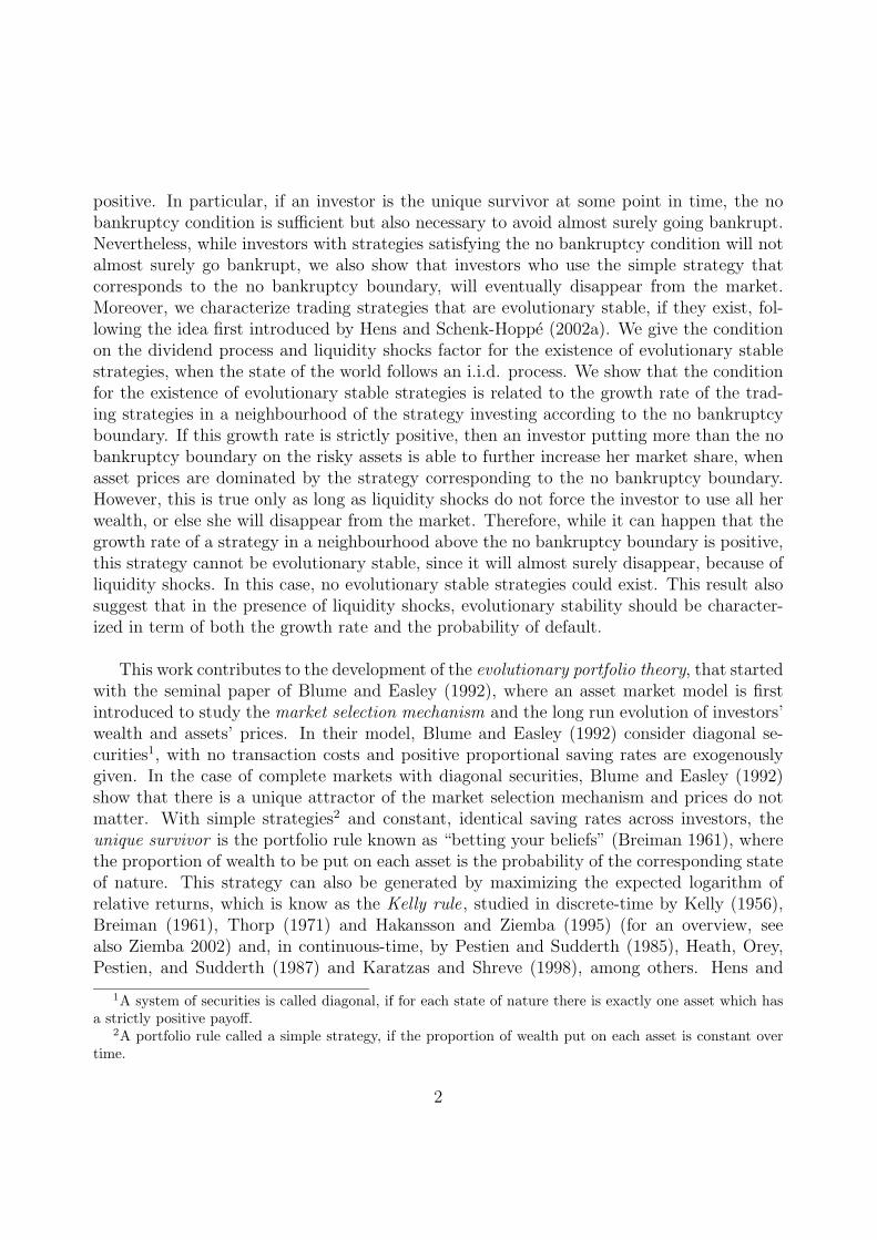
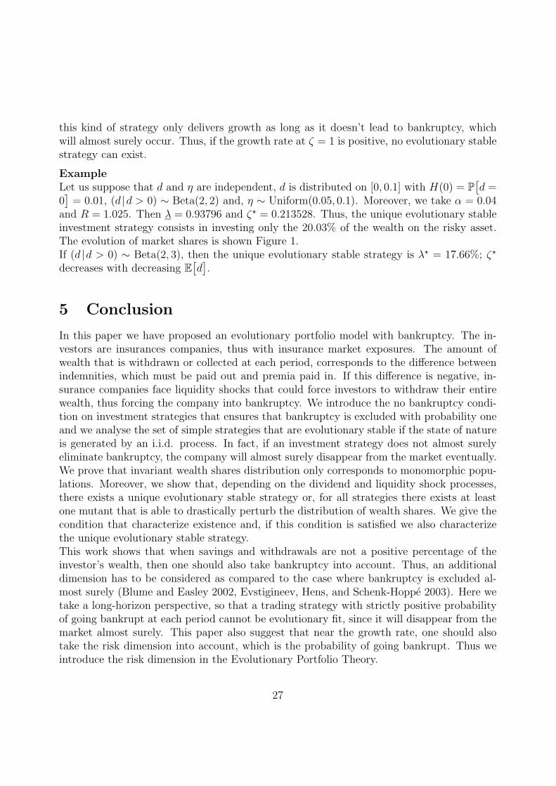
= 0.01, (d |d > 0) ∼ Beta(2, 2) and, η ∼ Uniform(0.05, 0.1). Moreover, we take α = 0.04and R = 1.025. Then λ = 0.93796 and ζ⋆ = 0.213528. Thus, the unique evolutionary stableinvestment strategy consists in investing only the 20.03% of the wealth on the risky asset.The evolution of market shares is shown Figure 1.If (d |d > 0) ∼ Beta(2, 3), then the unique evolutionary stable strategy is λ⋆ = 17.66%; ζ⋆

decreases with decreasing E[d].

5 Conclusion

In this paper we have proposed an evolutionary portfolio model with bankruptcy. The in-vestors are insurances companies, thus with insurance market exposures. The amount ofwealth that is withdrawn or collected at each period, corresponds to the difference betweenindemnities, which must be paid out and premia paid in. If this difference is negative, in-surance companies face liquidity shocks that could force investors to withdraw their entirewealth, thus forcing the company into bankruptcy. We introduce the no bankruptcy condi-tion on investment strategies that ensures that bankruptcy is excluded with probability oneand we analyse the set of simple strategies that are evolutionary stable if the state of natureis generated by an i.i.d. process. In fact, if an investment strategy does not almost surelyeliminate bankruptcy, the company will almost surely disappear from the market eventually.We prove that invariant wealth shares distribution only corresponds to monomorphic popu-lations. Moreover, we show that, depending on the dividend and liquidity shock processes,there exists a unique evolutionary stable strategy or, for all strategies there exists at leastone mutant that is able to drastically perturb the distribution of wealth shares. We give thecondition that characterize existence and, if this condition is satisfied we also characterizethe unique evolutionary stable strategy.This work shows that when savings and withdrawals are not a positive percentage of theinvestor’s wealth, then one should also take bankruptcy into account. Thus, an additionaldimension has to be considered as compared to the case where bankruptcy is excluded al-most surely (Blume and Easley 2002, Evstigineev, Hens, and Schenk-Hoppe 2003). Here wetake a long-horizon perspective, so that a trading strategy with strictly positive probabilityof going bankrupt at each period cannot be evolutionary fit, since it will disappear from themarket almost surely. This paper also suggest that near the growth rate, one should alsotake the risk dimension into account, which is the probability of going bankrupt. Thus weintroduce the risk dimension in the Evolutionary Portfolio Theory.

27

(a)

0 20 40 60 80 100

Time

0.0

0.2

0.4

0.6

0.8

1.0

Wea

lth s

hare

s

(b)

0 20 40 60 80 100

Time

0.0

0.2

0.4

0.6

0.8

1.0

Wea

lth s

hare

s

Figure 1: Evolution of market shares, for the λ⋆ strategy of Theorem 2 (full line), the strategyλ (dotted line), the risk free strategy (dashed-dotted line), and a randomly chosen strategyin (0, λ) (dashed line). In figure (a) all investors have the same initial wealth, while in figure(b) the strategy λ⋆ initially possesses only the 2% of the market capital.

28

References

Arnold, L. (1998): Random Dynamical Systems. Springer Verlag, Berlin.

Artzner, P., F. Delbaen, J.-M. Eber, and D. Heath (1997): “Thinking Coherently,”Risk, 10(11), 68–71.

Blume, L., and D. Easley (1992): “Evolution and Market Behavior,” Journal of Eco-nomic Theory, 58(1), 9–40.

(2002): “If You’re So Smart, Why Aren‘t You Rich? Belief Selection in Completeand Incomplete Markets,” Working paper, Department of Economics, Cornell University.

Breiman, L. (1961): “Optimal Gambling Systems For Favorable Games,” in Fourth Berke-ley Symposium on Mathematical Statistic and Probability, vol. 1, pp. 65–78, Berkeley.University of California Press.

Browne, S. (1997): “Survival and Growth with a Liability: Optimal Portfolio Strategiesin Continuous Time,” Mathematics of Operation Research, 22(2), 468–493.

(1999): “Reaching Goals by a Deadline: Digital Options and Continuous-TimeActive Portfolio Management,” Advances in Applied Probability, 31(2), 551–577.

Carino, D., D. Myers, and W. Ziemba (1998): “Concepts, Technical Issues, and Usesof the Russel-Yasuda Kasai Financial Planning Model,” Operations Research, 46, 449–462.

Carino, D., and W. Ziemba (1998): “Formulation of the Russel-Yasuda Kasi FinancialPlanning Model,” Operations Research, 46, 433–449.

Ceccarelli, S. (2002): “Insolvency Risk in the Italian Non-Life Insurance Companies. AnEmpirical Analysis Based on a Cash Flow Simulation Model,” Working paper, SupervisoryCommission on Pension Funds (COVIP), Rome.

Davis, P. (2001): “Portfolio Regulation of Life Insurance Companies and Pension Funds,”Working paper No. PI-0101, The Pensions Institute, Birkbeck College.

Embrechts, P. (1996): “Actuarial Versus Financial Pricing of Insurance,” Working paperNo. 96-17, The Wharton School, University of Pennsylvania.

Embrechts, P., E. De Giorgi, F. Lindskog, and A. McNeil (2002): “Audit of theSwiss Re Group Risk Model,” Unpublished report for Swiss Re.

Evstigineev, I., T. Hens, and K. Schenk-Hoppe (2003): “Evolutionary Stable StockMarkets,” Working paper No. 84, NCCR FINRISK Working paper series.

29

Evstigneev, I., T. Hens, and K. Schenk-Hoppe (2002): “Market Selection of FinancialTrading Strategies: Global Stability,” Mathematical Finance, 12(4), 329–339.

Feller, W. (1971): An Introduction to Probability Theory and Its Applications, vol. 2.Wiley, New York.

Hakansson, N., and W. Ziemba (1995): “Capital Growth Theory,” in Handbooks inOperations Research and Management Science, ed. by R. Jarrow, V. Maksimovic, and

W. Ziemba, vol. 9, pp. 65–86. Elsevier, Amsterdam.

Heath, D., S. Orey, W. Pestien, and W. Sudderth (1987): “Minimizing or Maxi-mizing the Expected Time to Reach Zero,” SIAM Journal of Control and Optimization,25(1), 195–205.

Hens, T., and K. Schenk-Hoppe (2002a): “Evolution of Portfolio Rules in IncompleteMarkets,” Working paper No. 74, Institute for Empirical Research in Economics, Univer-sity of Zurich.

Hens, T., and K. Schenk-Hoppe (2002b): “Markets Do Not Select For a LiquidityPreference as Behaviour Towards Risk,” Working paper No. 139, Institute for EmpiricalResearch in Economics, University of Zurich.

Horn, R., and C. Johnson (1985): Matrix Analysis. Cambridge University Press, Cam-bridge UK.

Karatzas, I., and S. Shreve (1998): Methods of Mathematical Finance. Springer-Verlag,New York.

Kelly, J. (1956): “A New Interpretation of Information Rate,” Bell System TechnicalJournal, 35, 917–926.

Leippold, M., P. Vanini, and F. Trojani (2003): “Equilibrium Impact of Value-at-RiskRegulation,” Working paper, University of Zurich and Universita della Svizzera Italiana.

Liu, J., F. A. Longstaff, and J. Pan (2003): “Dynamic Asset Allocation With EventRisk,” Journal of Finance, 58(1), 231–259.

Lucas, R. (1978): “Asset Prices in an Exchange Economy,” Econometrica, 46(6), 1429–1445.

Norberg, R., and B. Sundt (1985): “Draft on a System for Solvency Control in Non-LifeInsurance,” ASTIN Bulletin, 15(2), 150–169.

Pestien, V., and W. Sudderth (1985): “Continuous-Time Red and Black: How toControl a Diffusion to a Goal,” Mathematics of Operations Research, 10(4), 599–611.

30

Sandroni, A. (2000): “Do Markets Favor Agents Able to Make Accurate Predictions?,”Econometrica, 68(6), 1303–1341.

Schnieper, R. (1993): “The Insurance of Catastrophe Risks,” SCOR Notes, April 1993.

Thorp, E. (1971): “Portfolio Choice and the Kelly Criterion,” in Stochastic Models inFinance, ed. by W. Ziemba, and R. Vickson, pp. 599–619. Academic Press, New York.

Zhao, Y., and W. Ziemba (2000): “A Dynamic Asset Allocation Model with DownsideRisk Control,” The Journal of Risk, 3(1), 91–113.

Ziemba, W. (2002): “The Capital Growth Theory of Investment: Part I,” Willmott Maga-zine, December, 16–18.

6 Appendix

6.1 Existence and uniqueness of δit and Pt+1

For the sake of simplicity we drop the index t from the notation of equations (7) and (8).Using the expression (7) for δi in (8), we obtain

P = µ +∑

i

(σ θi

µ + σ θi − P− 1

)

αi wi,

where θi = F−1(1 − ǫi). Let f : [0, miniµ + σ θi) → R be defined by f(P ) = µ +∑

i

(σ θi

µ+σ θi−P− 1

)

αi wi. f is well defined on [0, miniµ+σ θi) and continuous differentiable,

with f ′(P ) =∑

iσ θi

(µ+σ θi−P )2αi wi > 0, f ′′(P ) =

∑

i2 σ θi

(µ+σ θi−P )3αi wi > 0, i.e. f is strictly

increasing and convex. Moreover, f(P ) ր ∞ as P ր miniµ + σ θi and

f(0) = µ +∑

i

(σ θi

µ + σ θi− 1

)

αi wi = µ − µ∑

i

αi wi

µ + σ θi

= µ − µ∑

i

δi|P=0

︸ ︷︷ ︸

=1

= 0,

f ′(0) =∑

i

σ θi αi wi

(µ + σ θi)2≤ max

i

σ θi

µ + σ θi

∑

i

αi wi

µ + σ θi

︸ ︷︷ ︸

=1

< 1,

since µ > 0. Thus f(P ) ≥ 0 and it possesses exactly two fixed points: P = 0 and P ⋆ ∈(0, miniµ + σ θi). Therefore, there is a unique premium P ∗ > 0 which satisfies equations(7) and (8). Moreover, by equation (7), δi is also uniquely defined for all i.

31

-

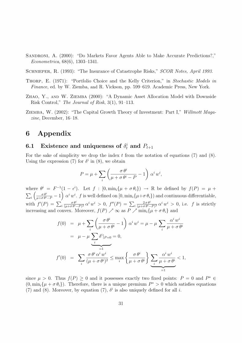
6

b´

´´

´´

´´

´´

´´

´´

´´

´´

´

0

f

b

P ∗

Figure 2: Proof of the existence and uniqueness of equilibrium insurance premium. Thedemand function f(P ) has one strictly positive fixed point P ∗.

6.2 Derivation of the wealth dynamics

wit+1 = Ai

t+1 +Bi

t

1 −∑

j λjt+1 Bj

t

∑

j

λjt+1 Aj

t

= Ait+1 +

λit w

it

∑

j λjt wj

t −∑

j λjt+1 λj

t wjt

∑

j

λjt+1 Aj

t

= wit

[

R (1 − λit) +

λit

λTt wt

dt+1 Wt − (ηt+1 − β + α)

+λit

∑

j wjtλ

jt+1

(

R (1 − λjt) +

λjt

λTt wt

dt+1 Wt − (ηt+1 − β + α))

∑

j(1 − λjt+1) λj

t wjt

32

Thus

wit+1 =

wit

λTt wt

[R (1 − λi

t) λTt wt + λi

tdt+1 Wt − (ηt+1 − β + α)λTt wt

+λit

∑

j wjtλ

jt+1

(R (1 − λj

t)λTt wt + λj

tdt+1Wt − (ηt+1 − β + α)λTt wt

)

∑

j(1 − λjt+1)λ

jtw

jt

]

=wi

t

λTt wt

1∑

j(1 − λjt+1)λ

jtw

jt

×

[∑

j

(1 − λjt+1)λ

jtw

jt

(R(1 − λi

t)λTt wt + λi

tdt+1Wt − (ηt+1 − β + α)λTt wt

)

+λit

(∑

j

wjtλ

jt+1

(R(1 − λj

t)λTt wt + λj

tdt+1Wt − (ηt+1 − β + α)λTt wt

)

)]

=wi

t∑

j(1 − λjt+1)λ

jtw

jt

×

[

dt+1Wtλit +

[R(1 − λi

t) − (ηt+1 − β + α)]

(

λTt wt +

∑

j

(λit − λj

t)λjt+1w

jt

)]

and therefore

wt+1 =wi

t∑

j(1 − λjt+1)λ

jtw

jt

×

[

dt+1Wtλit +

[R(λ − λi

t) + (η − ηt+1)]

(

λTt wt +

∑

j 6=i

(λit − λj

t)λjt+1 wj

t

)]

.

We use that

λ =R − η + β − α

R⇐⇒ R + β − α = R λ + η.

33