EVOLVING INSIDER THREAT DETECTION USING STREAM ANALYTICS ...lkhan/papers/uknw ThesisParveen.pdf · EVOLVING INSIDER THREAT DETECTION USING STREAM ANALYTICS AND BIG DATA Publication

EVOLVING INSIDER THREAT DETECTION USING

STREAM ANALYTICS AND BIG DATA

by

Pallabi Parveen

APPROVED BY SUPERVISORY COMMITTEE:

Dr. Bhavani Thuraisingham, Chair

Dr. Farokh B. Bastani

Dr. Weili Wu

Dr. Haim Schweitzer

Copyright c© 2013

Pallabi Parveen

All rights reserved

Dedicated to the Almighty Creator, the Most Gracious, the Most Merciful.



by

PALLABI PARVEEN, BS, MS

DISSERTATION

Presented to the Faculty of

The University of Texas at Dallas

in Partial Fulfillment

of the Requirements

for the Degree of

DOCTOR OF PHILOSOPHY IN

COMPUTER SCIENCE

THE UNIVERSITY OF TEXAS AT DALLAS

December 2013

ACKNOWLEDGMENTS

First and foremost, all praises to Almighty God for allowing me to write this dissertation.

Second, I would like to express my gratitude to my PhD advisor, Professor Bhavani Thu-

raisingham, for her constant support during my PhD studies. It was my great privilege that

she supported me as a research assistant during my MS studies (part of it) at UT Dallas.

During my graduate research, she gave me a lot of opportunity to work independently with

minimal interference.

Third, I would like to thank my wonderful committee members from the bottom of my heart.

In particular, during my job hunting, Professor Farokh Bastani was a great resource for me.

He was an immense help for preparing my job interview at VCE. During my graduate studies,

I took a number of courses with Dr. Haim Schweitzer, and I really enjoyed his teaching and

courses. I would like to also acknowledge Dr. Weili Wu and Dr. I-Ling Yen for their support

on various occasions.

Fourth, I would like to thank Dr. Robert Herklotz for his support. This work is supported

by the Air Force Office of Scientific Research, under grant FA-9550-09-1-0468 & FA9550-08-

1-0260.

Fifth, during my research work, I interacted with a number of co-workers, students and staff.

Their constant help shaped my research in the right direction. It would be an injustice if

I do not mention their names. They are: Dr. Jeffrey L. Partyka, Dr. James McGlothlin,

Dr. Lei Wang, Dr. Li Liu, Nate McDaniel, Vaibhav Khadilkar, Sanjay Bysani, Pratik P.

Desai, Rhonda Walls, Eric Modem and Norma Richardson. I would like to thank Amanda

Aiuvalasit and Wanda Trotta in the Office of the Graduate Dean for their time proofing my

dissertation.

v

Finally, I received a wonderful and constant support during my PhD journey from my family,

including parents, parents-in-law and sisters.

October 2013

vi

PREFACE

This dissertation was produced in accordance with guidelines which permit the inclusion as

part of the dissertation the text of an original paper or papers submitted for publication.

The dissertation must still conform to all other requirements explained in the “Guide for the

Preparation of Master’s Theses and Doctoral Dissertations at The University of Texas at

Dallas.” It must include a comprehensive abstract, a full introduction and literature review,

and a final overall conclusion. Additional material (procedural and design data as well as

descriptions of equipment) must be provided in sufficient detail to allow a clear and precise

judgment to be made of the importance and originality of the research reported.

It is acceptable for this dissertation to include as chapters authentic copies of papers already

published, provided these meet type size, margin, and legibility requirements. In such cases,

connecting texts which provide logical bridges between different manuscripts are mandatory.

Where the student is not the sole author of a manuscript, the student is required to make an

explicit statement in the introductory material to that manuscript describing the student’s

contribution to the work and acknowledging the contribution of the other author(s). The

signatures of the Supervising Committee which precede all other material in the dissertation

attest to the accuracy of this statement.

vii



Publication No.

Pallabi Parveen, PhDThe University of Texas at Dallas, 2013

Supervising Professor: Dr. Bhavani Thuraisingham

Evidence of malicious insider activity is often buried within large data streams, such as

system logs accumulated over months or years. Ensemble-based stream mining leverages

multiple classification models to achieve highly accurate anomaly detection in such streams,

even when the stream is unbounded, evolving, and unlabeled. This makes the approach

effective for identifying insiders who attempt to conceal their activities by varying their

behaviors over time.

This dissertation applies ensemble-based stream mining, supervised and unsupervised learn-

ing, and graph-based anomaly detection to the problem of insider threat detection. It

demonstrates that the ensemble-based approach is significantly more effective than tradi-

tional single-model methods, supervised learning outperforms unsupervised learning, and

increasing the cost of false negatives correlates to higher accuracy. It shows effectiveness

over non sequence data.

For sequence data, this dissertation proposes and tests an unsupervised, ensemble based

learning algorithm that maintains a compressed dictionary of repetitive sequences found

viii

throughout dynamic data streams of unbounded length to identify anomalies. In unsuper-

vised learning, compression-based techniques are used to model common behavior sequences.

This results in a classifier exhibiting a substantial increase in classification accuracy for data

streams containing insider threat anomalies. This ensemble of classifiers allows the un-

supervised approach to outperform traditional static learning approaches and boosts the

effectiveness over supervised learning approaches. One of the bottlenecks to construct com-

press dictionary is scalability. For this, an efficient solution is proposed and implemented

using Hadoop and MapReduce framework.

We could extend the work in the following directions. First, we will build a full fledge system

to capture user input as stream using apache flume and store it on the Hadoop distributed

file system (HDFS) and then apply our approaches. Next, we will apply MapReduce to

calculate edit distance between patterns for a particular user’s command sequence data.

ix

TABLE OF CONTENTS

ACKNOWLEDGMENTS . . . . . . . . . . . . . . . . . . . . . . . . . . . . . . . . . v

PREFACE . . . . . . . . . . . . . . . . . . . . . . . . . . . . . . . . . . . . . . . . . vii

ABSTRACT . . . . . . . . . . . . . . . . . . . . . . . . . . . . . . . . . . . . . . . . viii

LIST OF FIGURES . . . . . . . . . . . . . . . . . . . . . . . . . . . . . . . . . . . . xiii

LIST OF TABLES . . . . . . . . . . . . . . . . . . . . . . . . . . . . . . . . . . . . . xv

CHAPTER 1 INTRODUCTION . . . . . . . . . . . . . . . . . . . . . . . . . . . . 1

1.1 Sequence Stream Data . . . . . . . . . . . . . . . . . . . . . . . . . . . . . . 3

1.2 Big Data Issue . . . . . . . . . . . . . . . . . . . . . . . . . . . . . . . . . . 4

1.3 Contribution . . . . . . . . . . . . . . . . . . . . . . . . . . . . . . . . . . . . 4

1.4 Organization . . . . . . . . . . . . . . . . . . . . . . . . . . . . . . . . . . . 6

CHAPTER 2 RELATED WORK . . . . . . . . . . . . . . . . . . . . . . . . . . . . 8

2.1 Insider Threat and Stream Mining . . . . . . . . . . . . . . . . . . . . . . . . 8

2.1.1 Stream Mining . . . . . . . . . . . . . . . . . . . . . . . . . . . . . . 12

2.2 Big Data: Scalability Issue . . . . . . . . . . . . . . . . . . . . . . . . . . . . 15

2.2.1 With Regard to Big Data Management . . . . . . . . . . . . . . . . . 15

2.2.2 With Regard to Big Data Analytics . . . . . . . . . . . . . . . . . . . 16

CHAPTER 3 ENSEMBLE-BASED INSIDER THREAT DETECTION . . . . . . . 18

3.1 Ensemble Learning . . . . . . . . . . . . . . . . . . . . . . . . . . . . . . . . 19

3.1.1 Ensemble for Unsupervised Learning . . . . . . . . . . . . . . . . . . 22

3.1.2 Ensemble for Supervised Learning . . . . . . . . . . . . . . . . . . . . 24

CHAPTER 4 DETAILS OF LEARNING CLASSES . . . . . . . . . . . . . . . . . . 26

4.1 Supervised Learning . . . . . . . . . . . . . . . . . . . . . . . . . . . . . . . 26

4.2 Unsupervised Learning . . . . . . . . . . . . . . . . . . . . . . . . . . . . . . 27

4.2.1 GBAD-MDL . . . . . . . . . . . . . . . . . . . . . . . . . . . . . . . 28

4.2.2 GBAD-P . . . . . . . . . . . . . . . . . . . . . . . . . . . . . . . . . . 28

x

4.2.3 GBAD-MPS . . . . . . . . . . . . . . . . . . . . . . . . . . . . . . . . 29

CHAPTER 5 EXPERIMENTS AND RESULTS . . . . . . . . . . . . . . . . . . . . 30

5.1 Dataset . . . . . . . . . . . . . . . . . . . . . . . . . . . . . . . . . . . . . . 30

5.2 Experimental Setup . . . . . . . . . . . . . . . . . . . . . . . . . . . . . . . . 33

5.2.1 Supervised Learning . . . . . . . . . . . . . . . . . . . . . . . . . . . 33

5.2.2 Unsupervised Learning . . . . . . . . . . . . . . . . . . . . . . . . . . 34

5.3 Results . . . . . . . . . . . . . . . . . . . . . . . . . . . . . . . . . . . . . . . 36

5.3.1 Supervised Learning . . . . . . . . . . . . . . . . . . . . . . . . . . . 36

5.3.2 Unsupervised Learning . . . . . . . . . . . . . . . . . . . . . . . . . . 38

CHAPTER 6 INSIDER THREAT DETECTION FOR SEQUENCE DATA . . . . . 42

6.1 Model Update . . . . . . . . . . . . . . . . . . . . . . . . . . . . . . . . . . . 45

6.2 Unsupervised Stream based Sequence Learning (USSL) . . . . . . . . . . . . 46

6.2.1 Construct the LZW dictionary by selecting the patterns in the datastream . . . . . . . . . . . . . . . . . . . . . . . . . . . . . . . . . . . 51

6.2.2 Constructing the Quantized Dictionary . . . . . . . . . . . . . . . . . 51

6.3 Anomaly Detection (Testing) . . . . . . . . . . . . . . . . . . . . . . . . . . 53

6.4 Complexity Analysis . . . . . . . . . . . . . . . . . . . . . . . . . . . . . . . 54

CHAPTER 7 EXPERIMENTS AND RESULTS FOR SEQUENCE DATA . . . . . 56

7.1 Dataset . . . . . . . . . . . . . . . . . . . . . . . . . . . . . . . . . . . . . . 56

7.2 Concept Drift in the training set . . . . . . . . . . . . . . . . . . . . . . . . . 57

7.3 Result . . . . . . . . . . . . . . . . . . . . . . . . . . . . . . . . . . . . . . . 62

7.3.1 Choice of Ensemble Size . . . . . . . . . . . . . . . . . . . . . . . . . 63

CHAPTER 8 SCALABILIY USING HADOOP AND MAPREDUCE . . . . . . . . 68

8.1 Hadoop Map Reduce Background . . . . . . . . . . . . . . . . . . . . . . . . 68

8.2 Scalable LZW and Quantized Dictionary Construction using Map Reduce Job 71

8.2.1 Two MapReduce Job Approach (2MRJ) . . . . . . . . . . . . . . . . 72

8.2.2 1MRJ:1 MR Job . . . . . . . . . . . . . . . . . . . . . . . . . . . . . 75

8.3 Experimental Setup and Results . . . . . . . . . . . . . . . . . . . . . . . . . 80

8.3.1 Hadoop Cluster . . . . . . . . . . . . . . . . . . . . . . . . . . . . . . 80

xi

8.3.2 Big Dataset for Insider Threat Detection . . . . . . . . . . . . . . . . 80

8.3.3 Results for Big Data Set Related to Insider Threat Detection . . . . . 81

CHAPTER 9 CONCLUSIONS AND FUTURE WORK . . . . . . . . . . . . . . . . 88

9.1 Conclusion . . . . . . . . . . . . . . . . . . . . . . . . . . . . . . . . . . . . . 88

9.2 Future Work . . . . . . . . . . . . . . . . . . . . . . . . . . . . . . . . . . . . 89

9.2.1 Incorporate User Feedback . . . . . . . . . . . . . . . . . . . . . . . . 90

9.2.2 Collusion Attack . . . . . . . . . . . . . . . . . . . . . . . . . . . . . 90

9.2.3 Additional Experiment . . . . . . . . . . . . . . . . . . . . . . . . . . 90

9.2.4 Anomaly Detection in Social Network and Author Attribution . . . . 91

9.2.5 Stream mining as a Big data mining problem . . . . . . . . . . . . . 91

REFERENCES . . . . . . . . . . . . . . . . . . . . . . . . . . . . . . . . . . . . . . . 94

VITA

xii

LIST OF FIGURES

1.1 Contribution in Visual Form . . . . . . . . . . . . . . . . . . . . . . . . . . . . . 5

3.1 Concept drift in stream data . . . . . . . . . . . . . . . . . . . . . . . . . . . . . 19

3.2 Ensemble classification . . . . . . . . . . . . . . . . . . . . . . . . . . . . . . . . 20

4.1 A graph with a normative substructure (boxed) and anomalies (shaded) . . . . . 27

5.1 A sample system call record from the MIT Lincoln dataset . . . . . . . . . . . . 31

5.2 Feature set extracted from Figure 5.1 . . . . . . . . . . . . . . . . . . . . . . . . 31

5.3 A token subgraph . . . . . . . . . . . . . . . . . . . . . . . . . . . . . . . . . . . 32

5.4 Accuracy by FN Cost . . . . . . . . . . . . . . . . . . . . . . . . . . . . . . . . . 38

5.5 Total Cost by FN Cost . . . . . . . . . . . . . . . . . . . . . . . . . . . . . . . . 38

5.6 The effect of q on runtimes for fixed K = 6 on dataset A . . . . . . . . . . . . . 39

5.7 The effect of K on runtimes for fixed q = 4 on dataset A . . . . . . . . . . . . . 39

5.8 The effect of q on TP rates for fixed K = 6 on dataset A . . . . . . . . . . . . . 39

5.9 The effect of K on TP rates for fixed q = 4 on dataset A . . . . . . . . . . . . . 39

5.10 The effect of q on FP rates for fixed K = 6 on dataset A . . . . . . . . . . . . . 40

6.1 Example of Sequence Data related to Movement Pattern . . . . . . . . . . . . . 43

6.2 Concept drift in stream data . . . . . . . . . . . . . . . . . . . . . . . . . . . . . 44

6.3 Unsupervised stream sequence learning using incremental learning . . . . . . . . 46

6.4 Details block diagram of incremental learning . . . . . . . . . . . . . . . . . . . 47

6.5 Ensemble based unsupervised stream sequence learning . . . . . . . . . . . . . . 48

6.6 Unsupervised Stream based Sequence Learning(USSL)from a chunk in Ensemblebased case . . . . . . . . . . . . . . . . . . . . . . . . . . . . . . . . . . . . . . . 48

6.7 Quantization of dictionary . . . . . . . . . . . . . . . . . . . . . . . . . . . . . . 50

7.1 Pictorial Representation for Anomalous Data Generation Process . . . . . . . . 58

7.2 Comparison between NB-INC vs. our optimized model, USSL-GG in terms of TPR 64

7.3 Comparison between NB-INC vs. our optimized model, USSL-GG in terms of FPR 64

xiii

7.4 Comparison of USSL-GG across multiple drifts and ensemble sizes in terms of TPR 65

7.5 Comparison of USSL-GG across multiple drifts and ensemble sizes in terms of FPR 65

7.6 Comparison of USSL-GG across multiple drifts and ensemble sizes in terms ofAccuracy . . . . . . . . . . . . . . . . . . . . . . . . . . . . . . . . . . . . . . . 66

7.7 Comparison of USSL-GG across multiple drifts and ensemble sizes in terms of F1measure . . . . . . . . . . . . . . . . . . . . . . . . . . . . . . . . . . . . . . . . 67

7.8 Comparison of USSL-GG across multiple drifts and ensemble sizes in terms of F2measure . . . . . . . . . . . . . . . . . . . . . . . . . . . . . . . . . . . . . . . . 67

8.1 Word count example using MapReduce . . . . . . . . . . . . . . . . . . . . . . . 70

8.2 Approaches for scalable LZW and quantized dictionary construction using MapRe-duce Job . . . . . . . . . . . . . . . . . . . . . . . . . . . . . . . . . . . . . . . . 71

8.3 First MapReduce job for scalable LZW construction in 2MRJ approach . . . . . 72

8.4 Second MapReduce job for quantized dictionary construction in 2MRJ approach 73

8.5 1MRJ: 1 MR Job approach for scalable LZW and quantized dictionary construction 82

8.6 Time Taken for Varying Number of HDFS block size in 1MRJ . . . . . . . . . . 85

8.7 Time Taken for Varying Number of Reducer in 1MRJ . . . . . . . . . . . . . . . 85

xiv

LIST OF TABLES

2.1 Capabilities and focuses of various approaches for Non Sequence Data . . . . . . 11

2.2 Capabilities and focuses of various approaches for Sequence Data . . . . . . . . 14

5.1 Dataset statistics after filtering and attribute extraction . . . . . . . . . . . . . 34

5.2 Exp. A: One Class vs. Two Class SVM . . . . . . . . . . . . . . . . . . . . . . . 35

5.3 Exp. B: Updating vs. Non Updating Stream Approach . . . . . . . . . . . . . . 35

5.4 Summary of data subset A (Selected/Partial) . . . . . . . . . . . . . . . . . . . 35

5.5 Impact of FN Cost . . . . . . . . . . . . . . . . . . . . . . . . . . . . . . . . . . 38

5.6 Impact of fading factor λ (weighted voting) . . . . . . . . . . . . . . . . . . . . 40

5.7 Supervised vs. Non Supervised Learning Approach on dataset A . . . . . . . . . 41

6.1 Time Complexity of Quantization Dictionary Construction . . . . . . . . . . . . 54

7.1 Description of Dataset . . . . . . . . . . . . . . . . . . . . . . . . . . . . . . . . 57

7.2 NB-INC vs. USSL-GG for various drift values on TPR and FPR . . . . . . . . . 63

7.3 NB-INC vs. USSL-GG for various drift values on Accuracy and runtime . . . . 63

7.4 NB-INC vs. USSL-GG for various drift values on F1 and F2 Measure . . . . . . 63

8.1 Time Performance of 2MRJ vs. 1MRJ for varying number of reducers . . . . . . 83

8.2 Time performance of mapper for LZW dictionary construction with varying par-tition size in 2MRJ . . . . . . . . . . . . . . . . . . . . . . . . . . . . . . . . . . 84

8.3 Details of LZW dictionary construction and quantization using MapReduce in2MRJ on OD dataset . . . . . . . . . . . . . . . . . . . . . . . . . . . . . . . . . 84

8.4 Time performance of 1MRJ for varying reducer and HDFS block Size on DBD . 84

xv

CHAPTER 1

INTRODUCTION

There is a growing consensus within the intelligence community that malicious insiders

are perhaps the most potent threats to information assurance in many or most organiza-

tions (Brackney and Anderson, 2004; Hampton and Levi, 1999; Matzner and Hetherington,

2004; Salem and Stolfo, 2011). One traditional approach to the insider threat detection prob-

lem is supervised learning, which builds data classification models from training data. Unfor-

tunately, the training process for supervised learning methods tends to be time-consuming

and expensive, and generally requires large amounts of well-balanced training data to be

effective. In our experiments we observe that less than 3% of the data in realistic datasets

for this problem are associated with insider threats (the minority class); over 97% of the

data is associated with non-threats (the majority class). Hence, traditional support vec-

tor machines (SVM)(Chang and Lin, 2011; Manevitz and Yousef, 2002), trained from such

imbalanced data are likely to perform poorly on test datasets.

One-class SVMs (OCSVM)(Manevitz and Yousef, 2002) address the rare-class issue by

building a model that considers only normal data (i.e., non-threat data). During the testing

phase, test data is classified as normal or anomalous based on geometric deviations from the

model. However, the approach is only applicable to bounded-length, static data streams.

In contrast, insider threat-related data is typically continuous, and threat patterns evolve

over time. In other words, the data is a stream of unbounded length. Hence, effective

classification models must be adaptive (i.e., able to cope with evolving concepts) and highly

efficient in order to build the model from large amounts of evolving data.

Data that is associated with insider threat detection and classification is often continuous.

In these systems, the patterns of average users and insider threats can gradually evolve

1

2

over time. A novice programmer can develop his skills to become an expert programmer

over time. An insider threat can change his actions to more closely mimic legitimate user

processes. In either case, the patterns at either end of these developments can look drastically

different when compared directly to each other. These natural changes will not be treated

as anomalies in our approach. Instead, we classify them as natural concept drift. The

traditional static supervised and unsupervised methods raise unnecessary false alarms with

these cases because they are unable to handle them when they arise in the system. These

traditional methods encounter high false positive rates. Learning models must be adept in

coping with evolving concepts and highly efficient at building models from large amounts of

data to rapidly detecting real threats.

For these reasons, the insider threat problem can be conceptualized as a stream mining

problem that applies to continuous data streams. Whether using a supervised or unsu-

pervised learning algorithm, the method chosen must be highly adaptive to correctly deal

with concept drifts under these conditions. Incremental learning and Ensemble based learn-

ing (Masud, Chen, Gao, Khan, Aggarwal et al., 2010; Masud et al., 2011a; Masud, Gao et al.,

2008; Masud et al., 2013; Masud, Woolam et al., 2011; Masud et al., 2011b; Al-Khateeb, Ma-

sud, Khan, Aggarwal et al., 2012; Masud, Al-Khateeb et al., 2011; Masud,Chen, Gao, Khan,

Han and Thuraisingham, 2010) are two adaptive approaches in order to overcome this hin-

drance. An ensemble of K models that collectively vote on the final classification can reduce

the false negatives (FN) and false positives (FP) for a test set. As new models are created

and old ones updated to be more precise, the least accurate models are discarded to always

maintain an ensemble of exactly K current models.

An alternative approach to supervised learning is unsupervised learning, which can be

effectively applied to purely unlabeled data—i.e., data in which no points are explicitly

identified as anomalous or non-anomalous. Graph-based anomaly detection (GBAD) is one

important form of unsupervised learning (Cook and Holder, 2007; Eberle and Holder, 2007;

3

Cook and Holder, 2000), but has traditionally been limited to static, finite-length datasets.

This limits its application to streams related to insider threats, which tend to have unbounded

length and threat patterns that evolve over time. Applying GBAD to the insider threat

problem therefore requires that the models used be adaptive and efficient. Adding these

qualities allow effective models to be built from vast amounts of evolving data.

In this dissertation we cast insider threat detection as a stream mining problem and pro-

pose two methods (supervised and unsupervised learning) for efficiently detecting anomalies

in stream data (Parveen, McDaniel et al., 2013). To cope with concept-evolution, our super-

vised approach maintains an evolving ensemble of multiple OCSVM models (Parveen, Weger

et al., 2011). Our unsupervised approach combines multiple GBAD models in an ensemble

of classifiers (Parveen, Evans et al., 2011). The ensemble updating process is designed in

both cases to keep the ensemble current as the stream evolves. This evolutionary capability

improves the classifier’s survival of concept-drift as the behavior of both legitimate and ille-

gitimate agents varies over time. In experiments, we use test data that records system call

data for a large, Unix-based, multiuser system.

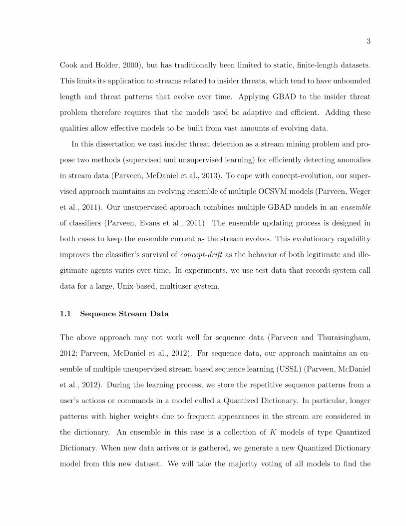
1.1 Sequence Stream Data

The above approach may not work well for sequence data (Parveen and Thuraisingham,

2012; Parveen, McDaniel et al., 2012). For sequence data, our approach maintains an en-

semble of multiple unsupervised stream based sequence learning (USSL) (Parveen, McDaniel

et al., 2012). During the learning process, we store the repetitive sequence patterns from a

user’s actions or commands in a model called a Quantized Dictionary. In particular, longer

patterns with higher weights due to frequent appearances in the stream are considered in

the dictionary. An ensemble in this case is a collection of K models of type Quantized

Dictionary. When new data arrives or is gathered, we generate a new Quantized Dictionary

model from this new dataset. We will take the majority voting of all models to find the

4

anomalous pattern sequences within this new data set. We will update the ensemble if the

new dictionary outperforms others in the ensemble and will discard the least accurate model

from the ensemble. Therefore, the ensemble always keeps the models current as the stream

evolves, preserving high detection accuracy as both legitimate and illegitimate behaviors

evolve over time. Our test data consists of real-time recorded user command sequences for

multiple users of varying experience levels and a concept drift framework to further exhibit

the practicality of this approach.

1.2 Big Data Issue

Quantized dictionary construction is time consuming. Scalability is a bottleneck here. We

exploit distributed computing to address this issue. There are two ways we can achieve this

goal. The first one is parallel computing with shared memory architecture that exploits

expensive hardware. The latter approach is distributing computing with shared nothing ar-

chitecture that exploits commodity hardware. For our case, we exploit the latter choice.

Here, we use MapReduce based framework to facilitate quantization using Hadoop Dis-

tributed File System (HDFS). We propose a number of algorithms to quantize dictionary.

For each of them we discuss the pros and cons and report performance results on a large

dataset.

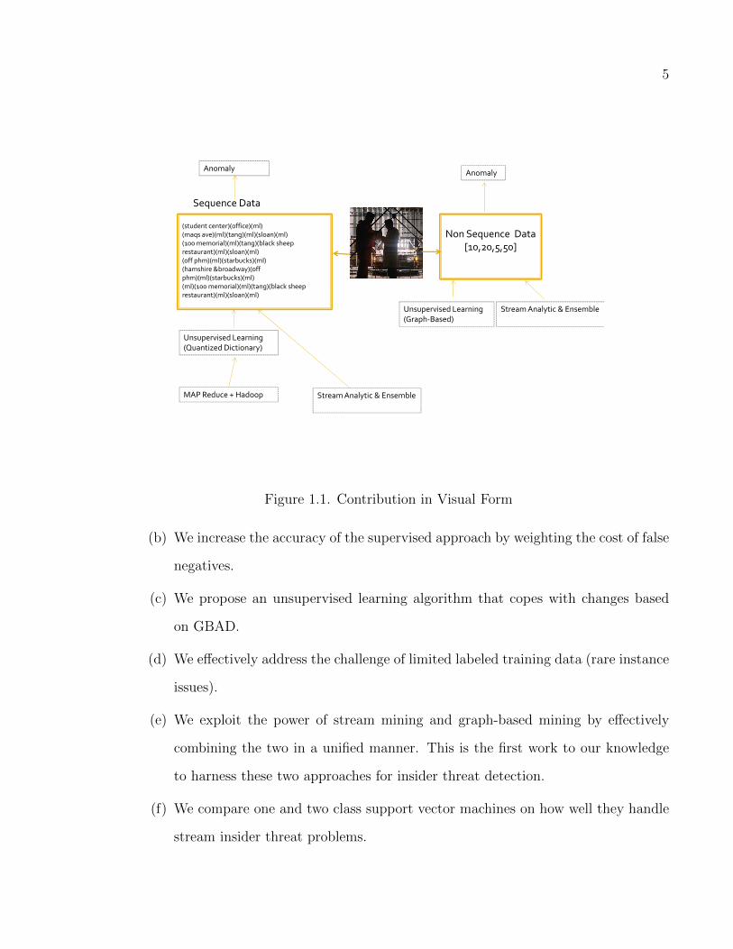
1.3 Contribution

The main contributions of this work can be summarized as follows (see Figure 1.1).

1. We show how stream mining can be effectively applied to detect insider threats.

2. With regard to Non sequence Data

(a) We propose a supervised learning solution that copes with evolving concepts using

one-class SVMs.

5

(student center)(office)(ml)(maqs ave)(ml)(tang)(ml)(sloan)(ml)(100 memorial)(ml)(tang)(black sheep restaurant)(ml)(sloan)(ml)(off phm)(ml)(starbucks)(ml)(hamshire &broadway)(off phm)(ml)(starbucks)(ml)(ml)(100 memorial)(ml)(tang)(black sheep restaurant)(ml)(sloan)(ml)

Sequence Data

Non Sequence Data [10,20,5,50]

AnomalyAnomaly

restaurant)(ml)(sloan)(ml)

MAP Reduce + Hadoop

Unsupervised Learning (Quantized Dictionary)

Stream Analytic & EnsembleUnsupervised Learning (Graph-Based)

Stream Analytic & Ensemble

Figure 1.1. Contribution in Visual Form

(b) We increase the accuracy of the supervised approach by weighting the cost of false

negatives.

(c) We propose an unsupervised learning algorithm that copes with changes based

on GBAD.

(d) We effectively address the challenge of limited labeled training data (rare instance

issues).

(e) We exploit the power of stream mining and graph-based mining by effectively

combining the two in a unified manner. This is the first work to our knowledge

to harness these two approaches for insider threat detection.

(f) We compare one and two class support vector machines on how well they handle

stream insider threat problems.

6

(g) We compare supervised and unsupervised stream learning approaches and show

which has superior effectiveness using real-world data.

3. With regard to Sequence Data

(a) For sequence data, we propose a framework that exploits an unsupervised learning

(USSL) to find pattern sequences from successive user actions or commands using

stream based sequence learning.

(b) We effectively integrate multiple USSL models in an ensemble of classifiers to

exploit the power of ensemble based stream mining and sequence mining.

(c) We compare our approach with the supervised model for stream mining and show

the effectiveness of our approach in terms of TPR and FPR on a benchmark

dataset.

4. With regard to Big Data

(a) scalability is an issue to construct benign pattern sequences for quantized dictio-

nary. For this, we exploit MapReduce based framework and show effectiveness of

our work.

1.4 Organization

The remainder of the dissertation is organized as follows. Chapter 2 presents related work.

Chapter 3 presents our ensemble-based approaches to insider threat. Chapter 4 discusses

the background of supervised and unsupervised learning methods for anomaly detection.

Chapter 5 describes our experiments and testing methodology and presents our results and

findings on non sequence data. Chapter 6 presents our proposed unsupervised sequence

learning for anomaly detection on sequence data. Chapter 7 presents results of our approach

7

on sequence data. Chapter 8 presents scalability issue and solution for quantized dictionary

construction. Finally, Chapter 9 concludes with an assessment of the viability of stream

mining for real-world insider threat detection.

CHAPTER 2

RELATED WORK

Here, first we will present related work with regard to insider threat and stream mining area.

Next, we will present related work with regard to big data and analytics perspective.

2.1 Insider Threat and Stream Mining

Insider threat detection work has applied ideas from both intrusion detection and external

threat detection (Schonlau et al., 2001; Wang et al., 2003; Maxion, 2003; Schultz, 2002).

Supervised learning approaches collect system call trace logs containing records of normal

and anomalous behavior (Forrest et al., 1996; Hofmeyr et al., 1998; Nguyen et al., 2003;

Gao et al., 2004), extract n-gram features from the collected data, and use the extracted

features to train classifiers. Text classification approaches treat each system call as a word in

a bag-of-words model (Liao and Vemuri, 2002). Various attributes of system calls, including

arguments, object path, return value, and error status, have been exploited as features in

various supervised learning methods (Krugel et al., 2003; Tandon and Chan, 2003).

Hybrid high-order Markov chain models detect anomalies by identifying a signature be-

havior for a particular user based on their command sequences (Ju and Vardi, 2001). The

Probabilistic Anomaly Detection (PAD) algorithm (Stolfo et al., 2005) is a general purpose

algorithm for anomaly detection (in the windows environment) that assumes anomalies or

noise is a rare event in the training data. Masquerade detection is argued over by some

individuals. A number of detection methods were applied to a data set of ”truncated”

UNIX shell commands for 70 users (Schonlau et al., 2001). Commands were collected using

the UNIX acct auditing mechanism. For each user a number of commands were gathered

8

9

over a period of time. The detection methods were supervised by a multi-step Markovian

model and a combination of Bayes and Markov approaches. It was argued that the data

set was not appropriate for the masquerade detection task (Maxion, 2003). It was pointed

out that the period of data gathering varied greatly from user to user (from several days to

several months). Furthermore, commands were not logged in the order in which they were

typed. Instead, they were coalesced when the application terminated the audit mechanism.

This leads to the unfortunate consequence of possible faulty analysis of strict sequence data.

Therefore, in this proposed work we have not considered this dataset.

These approaches differ from our supervised approach in that these learning approaches

are static in nature and do not learn over evolving streams. In other words, stream character-

istics of data are not explored further. Hence, static learning performance may degrade over

time. On the other hand, our supervised approach will learn from evolving data streams.

Our proposed work is based on supervised learning and it can handle dynamic data or stream

data well by learning from evolving streams.

In anomaly detection, one class SVM algorithm is used (Stolfo et al., 2005). OCSVM

builds a model by training on normal data and then classifies test data as benign or anoma-

lous based on geometric deviations from that normal training data. For masquerade de-

tection, one class SVM training is as affective as two class training (Stolfo et al., 2005).

Investigations have been made into SVMs using binary features and frequency based fea-

tures. The one class SVM algorithm with binary features performed the best.

Recursive mining has been proposed to find frequent patterns (Szymanski and Zhang,

2004). One class SVM classifier were used for masquerade detection after the patterns were

encoded with unique symbols and all sequences rewritten with this new coding.

To the best of our knowledge there is no work that extends this OCSVM in a stream

domain. Although our approach relies on OCSVM, it is extended to the stream domain so

that it can cope with changes (Parveen, Weger et al., 2011; Parveen, McDaniel et al., 2013).

10

Past works have also explored unsupervised learning for insider threat detection, but only

to static streams to our knowledge (Liu et al., 2005; Eskin et al., 2002, 2000). Static graph

based anomaly detection (GBAD) approaches (Cook and Holder, 2007; Eberle and Holder,

2007; Cook and Holder, 2000; Yan and Han, 2002) represent threat and non-threat data as

a graph and apply unsupervised learning to detect anomalies. The minimum description

length (MDL) approach to GBAD has been applied to email, cell phone traffic, business

processes, and cybercrime datasets (Staniford-Chen et al., 1996; Kowalski et al., 2008). Our

work builds upon GBAD and MDL to support dynamic, evolving streams (Parveen, Evans

et al., 2011; Parveen, McDaniel et al., 2013).

Stream mining (Fan, 2004) is a relatively new category of data mining research that

applies to continuous data streams. In such settings, both supervised and unsupervised

learning must be adaptive in order to cope with data whose characteristics change over time.

There are two main approaches to adaptation: incremental learning (Domingos and Hulten,

2001; Davison and Hirsh, 1998) and ensemble-based learning (Masud, Chen, Gao, Khan,

Aggarwal et al., 2010; Masud et al., 2011a; Fan, 2004). Past work has demonstrated that

ensemble-based approaches are the more effective of the two, motivating our approach.

Ensembles have been used in the past to bolster the effectiveness of positive/negative

classification (Masud, Gao et al., 2008; Masud et al., 2011a). By maintaining an ensemble

of K models that collectively vote on the final classification, the number of false negatives

(FN) and false positives (FP) for a test set can be reduced. As better models are created,

poorer models are discarded to maintain an ensemble of size exactly K. This helps the

ensemble evolve with the changing characteristics of the stream and keeps the classification

task tractable.

A comparison of the above related works is summarized in Table 2.1. A more complete

survey is available in (Salem et al., 2008).

Insider threat detection work has utilized ideas from intrusion detection or external threat

detection areas (Schonlau et al., 2001; Wang et al., 2003). For example, supervised learning

11

Table 2.1. Capabilities and focuses of various approaches for Non Sequence Data

learn concept insider graphApproach ing drift threat based

(Hofmeyr et al., 1998) S 7 X 7

(Eskin et al., 2002) S X 7 7

(Liu et al., 2005) U 7 X 7

(Cook and Holder, 2007) GBAD U 7 X X(Masud, Gao et al., 2008) S X N/A N/A(Parveen, Evans et al., 2011) S/U X X X

has been applied to detect insider threats. System call traces from normal activity and

anomaly data are gathered (Hofmeyr et al., 1998); features are extracted from this data

using n-gram and finally, trained with classifiers. Authors (Liao and Vemuri, 2002) exploit

the text classification idea in the insider threat domain where each system call is treated

as a word in bag of words model. System call, and related attributes, arguments, object

path, return value and error status of each system call are served as features in various

supervised methods (Krugel et al., 2003; Tandon and Chan, 2003). A supervised model

based on hybrid high-order Markov chain model was adopted by researchers (Ju and Vardi,

2001). A signature behavior for a particular user based on the command sequences that the

user executed is identified and then anomaly is detected.

Schonlau et al. (Schonlau et al., 2001) applied a number of detection methods to a data

set of ”truncated” UNIX shell commands for 70 users. Commands were collected using the

UNIX acct auditing mechanism. For each user a number of commands were gathered over a

period of time. The detection methods are supervised based on multistep markovian model,

and combination of Bayes and Markov approach. Maxion et al. (Maxion, 2003) argued that

Schonlau data set was not appropriate for the masquerade detection task and created new

data set using Calgary dataset and apply static supervised model.

These approaches differ from our work in the following ways. These learning approaches

are static in nature and do not learn over evolving stream. In other words, stream charac-

teristics of data are not explored further. Hence, static learner performance may degrade

12

over time. On the other hand, our approach will learn from evolving data stream. In this

paper, we show that our approach is unsupervised and is as effective as supervised model

(incremental).

Researchers have explored unsupervised learning (Liu et al., 2005) for insider threat

detection. However, this learning algorithm is static in nature. Although our approach is

unsupervised, it learns at the same time from evolving stream over time, and more data will

be used for unsupervised learning.

In anomaly detection, one class support vector machine (SVM) algorithm (OCSVM)

is used. OCSVM builds a model from training on normal data and then classifies a test

data as benign or anomaly based on geometric deviations from normal training data. Wang

et al. (Wang et al., 2003) showed, for masquerade detection, one-class SVM training is as

effective as two-class training. The authors have investigated SVMs using binary features

and frequency based features. The one-class SVM algorithm with binary features performed

the best. To find frequent patterns, Szymanski et al. (Szymanski and Zhang, 2004) proposed

recursive mining, encoded the patterns with unique symbols, and rewrote the sequence using

this new coding. They used a one-class SVM classifier for masquerade detection. These

learning approaches are static in nature and do not learn over evolving stream.

2.1.1 Stream Mining

Stream mining is a new data mining area where data is continuous (Masud et al., 2013;

Masud, Woolam et al., 2011; Masud et al., 2011b; Al-Khateeb, Masud, Khan, Aggarwal et al.,

2012; Masud, Al-Khateeb et al., 2011; Masud,Chen, Gao, Khan, Han and Thuraisingham,

2010). In addition, characteristics of data may change over time (concept drift). Here,

supervised and unsupervised learning need to be adaptive to cope with changes. There are

two ways adaptive learning can be developed. One is incremental learning and the other is

ensemble-based learning. Incremental learning is used in user action prediction (Domingos

13

and Hulten, 2000), but not for anomaly detection. Davidson et al. (Davison and Hirsh, 1998)

introduced Incremental Probabilistic Action Modeling (IPAM), based on one-step command

transition probabilities estimated from the training data. The probabilities were continuously

updated with the arrival of a new command and modified with the usage of an exponential

decay scheme. However, the algorithm is not designed for anomaly detection.

Therefore, to the best of our knowledge, there is almost no work from other researchers

that handles insider threat detection in stream mining area. This is the first attempt to detect

insider threat using stream mining (Parveen, Evans et al., 2011; Parveen and Thuraisingham,

2012; Parveen, McDaniel et al., 2012).

Recently, unsupervised learning has been applied to detect insider threat in a data

stream (Parveen, McDaniel et al., 2013; Parveen, Weger et al., 2011). This work does

not consider sequence data for threat detection. Recall that sequence data is very common

in insider threat scenario. Instead, it considers data as graph/vector and finds normative

patterns and apply ensemble based technique to cope with changes. On the other hand,

in our proposed approach, we consider user command sequences for anomaly detection and

construct quantized dictionary for normal patterns.

Users’ repetitive daily or weekly activities may constitute user profiles. For example, a

user’s frequent command sequences may represent normative pattern of that user. To find

normative patterns over dynamic data streams of unbounded length is challenging due to the

requirement of one pass algorithm. For this, an unsupervised learning approach is used by

exploiting a compressed/quantized dictionary to model common behavior sequences. This

unsupervised approach needs to identify normal user behavior in a single pass (Parveen,

McDaniel et al., 2012; Parveen and Thuraisingham, 2012; Chua et al., 2011). One major

challenge with these repetitive sequences is their variability in length. To combat this prob-

lem, we generate a dictionary which will contain any combination of possible normative

patterns existing in the gathered data stream. In addition, we have incorporated power of

14

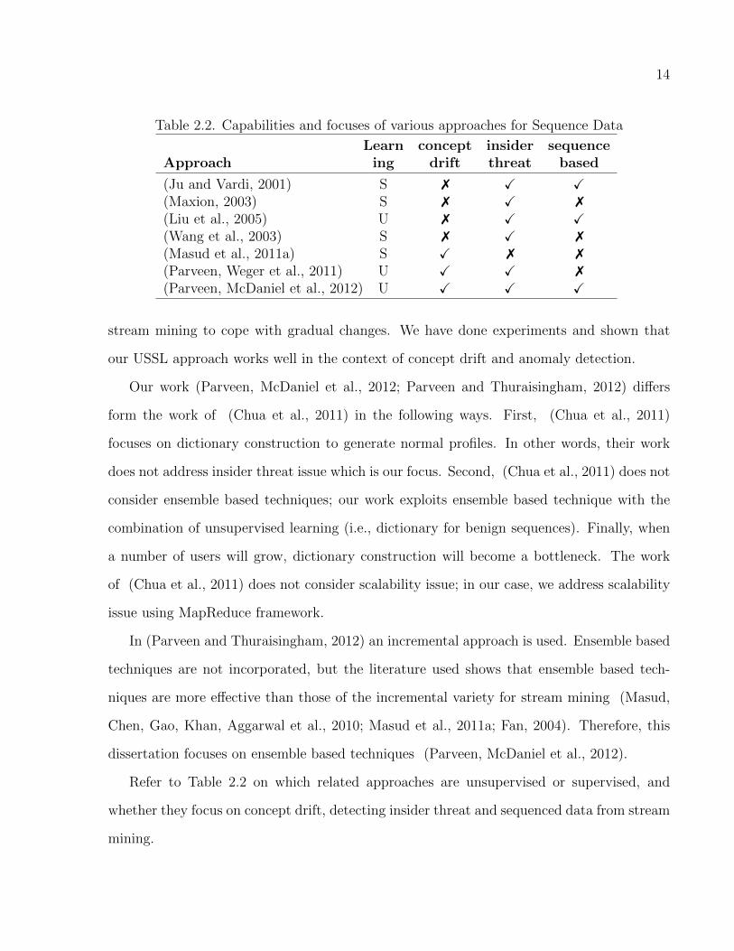
Table 2.2. Capabilities and focuses of various approaches for Sequence Data

Learn concept insider sequenceApproach ing drift threat based

(Ju and Vardi, 2001) S 7 X X(Maxion, 2003) S 7 X 7

(Liu et al., 2005) U 7 X X(Wang et al., 2003) S 7 X 7

(Masud et al., 2011a) S X 7 7

(Parveen, Weger et al., 2011) U X X 7

(Parveen, McDaniel et al., 2012) U X X X

stream mining to cope with gradual changes. We have done experiments and shown that

our USSL approach works well in the context of concept drift and anomaly detection.

Our work (Parveen, McDaniel et al., 2012; Parveen and Thuraisingham, 2012) differs

form the work of (Chua et al., 2011) in the following ways. First, (Chua et al., 2011)

focuses on dictionary construction to generate normal profiles. In other words, their work

does not address insider threat issue which is our focus. Second, (Chua et al., 2011) does not

consider ensemble based techniques; our work exploits ensemble based technique with the

combination of unsupervised learning (i.e., dictionary for benign sequences). Finally, when

a number of users will grow, dictionary construction will become a bottleneck. The work

of (Chua et al., 2011) does not consider scalability issue; in our case, we address scalability

issue using MapReduce framework.

In (Parveen and Thuraisingham, 2012) an incremental approach is used. Ensemble based

techniques are not incorporated, but the literature used shows that ensemble based tech-

niques are more effective than those of the incremental variety for stream mining (Masud,

Chen, Gao, Khan, Aggarwal et al., 2010; Masud et al., 2011a; Fan, 2004). Therefore, this

dissertation focuses on ensemble based techniques (Parveen, McDaniel et al., 2012).

Refer to Table 2.2 on which related approaches are unsupervised or supervised, and

whether they focus on concept drift, detecting insider threat and sequenced data from stream

mining.

15

2.2 Big Data: Scalability Issue

Stream data are continuously coming with high velocity and large size (Al-Khateeb, Masud,

Khan, and Thuraisingham, 2012). This conforms characteristics of big data.

”Big Data” is data whose scale, diversity, and complexity require new architecture, tech-

niques, algorithms, and analytics to manage it and extract value and hidden knowledge from

it. Therefore, big data researchers are looking for tools to manage, analyze, summarize, vi-

sualize, and discover knowledge from the collected data in a timely manner and in a scalable

fashion. Here, we will list some and discuss what problems we are solving in big data.

2.2.1 With Regard to Big Data Management

There are a number of techniques available that allow massively scalable data processing

over grids of inexpensive commodity hardware such as:

The Google File System (Chang et al., 2006; Dean and Ghemawat, 2008) is a scalable dis-

tributed file system that utilizes clusters of commodity hardware to facilitate data intensive

applications. The system is fault tolerance where failure of machine is norm due to usage of

commodity hardware. To cope with failure, data will replicated into multiple nodes. If one

node is failing, the system will utilize the other node where replicated data exists.

MapReduce (Chang et al., 2006; Dean and Ghemawat, 2008) is a programming model that

supports data-intensive applications in a parallel manner. MapReduce paradigm supports

map and reduce function. Map generates a set of intermediate key and value pairs and then

reduce function combines the results and deduces it. In fact, the map/reduce paradigm can

solve many real world problems as shown in (Chang et al., 2006; Dean and Ghemawat,

2008).

Hadoop (Bu et al., 2010; Xu et al., 2010; Abouzeid et al., 2009) is an open source apache

project that supports Google file system and mapReduce paradigm. Hadoop is widely used to

address scalability issue along with mapReduce. For example, with huge amount of semantic

16

web datasets, Husain et al. (Husain et al., 2009, 2010, 2011) showed that Hadoop can be

used to provide scalable queries. In addition, MapReduce technology has been exploited by

BioMANTA1 project (Ding et al., 2005) and SHARD 2.

Amazon develops Dynamo (DeCandia et al., 2007), a distributed key-value store. Dy-

namo does not support master-slave architecture which is supported by Hadoop. Nodes in

Dynamo communicate via a gossip network. To achieve high availability and performance,

Dynamo supports a model called eventual consistency by sacrificing rigorous consistency. In

eventual consistency, updates will be propagated to nodes in the cluster asynchronously and

a new version of the data will be produced for each update.

Google develops BigTable (Chang et al., 2006, 2008), column-oriented data storage sys-

tem. BigTable utilizes the Google File System and Chubby (Burrows, 2006), a distributed

lock service. BigTable is a distributed multi-dimensional sparse map based on row keys,

column names and time stamps.

Researchers (Abouzeid et al., 2009) exploited combining power of MapReduce and rela-

tional database technology.

2.2.2 With Regard to Big Data Analytics

There are handfuls of works related to big data analytics. For example, on one hand, some

researcher focus on generic analytics tool to address scalability issue. On the other hand,

other researcher focus on specific analytics problems.

With regard to tool, Mahout is an open source big data analytics to support classification,

clustering, and recommendation system for big data. In (Chu et al., 2006), researchers

customized well-known machine learning algorithms to take advantage of multicore machines

1http://www.itee.uq.edu.au/ eresearch/projects/biomanta

2http://www.cloudera.com/blog/2010/03/how-raytheon-researchers-are-using-hadoop-to-build-a-scalable-distributed-triple-store

17

and MapReduce programming paradigm. MapReduce has been widely used for mining

petabytes of data (Moretti et al., 2008).

With regard to specific problems, Al-Khateeb et al. (Al-Khateeb, Masud, Khan, and

Thuraisingham, 2012) and Haque et al. (Haque et al., 2013a,b) proposed scalable classifica-

tion over evolving stream by exploiting MapReduce and Hadoop framework. There are some

research works on parallel boosting with MapReduce. Palit et al. (Palit and Reddy, 2012)

proposed two parallel boosting algorithms, ADABOOST.PL and LOGITBOOST.PL.

CHAPTER 3

ENSEMBLE-BASED INSIDER THREAT DETECTION

Data relevant to insider threats is typically accumulated over many years of organization and

system operations, and is therefore best characterized as an unbounded data stream. Such a

stream can be partitioned into a sequence of discrete chunks ; for example, each chunk might

comprise a week’s worth of data.

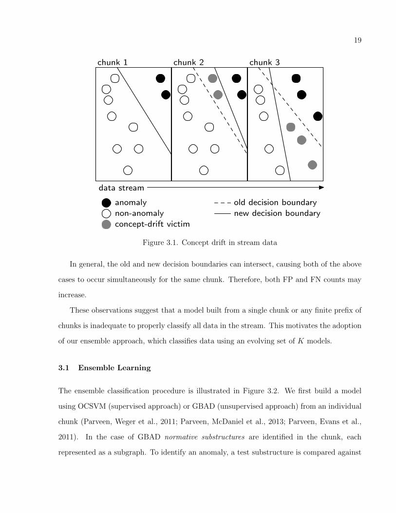
Figure 3.1 illustrates how a classifier’s decision boundary changes when such a stream

observes concept-drift. Each circle in the picture denotes a data point having , with unfilled

circles representing true negatives (TN) (i.e., non-anomalies) and solid circles representing

true positives (TP) (i.e., anomalies). The solid line in each chunk represents the decision

boundary for that chunk, while the dashed line represents the decision boundary for the

previous chunk.

Shaded circles are those that embody a new concept that has drifted relative to the

previous chunk. In order to classify these properly, the decision boundary must be adjusted

to account for the new concept. There are two possible varieties of misapprehension (false

detection):

1. The decision boundary of chunk 2 moves upward relative to chunk 1. As a result,

some non-anomalous data is incorrectly classified as anomalous, causing the FP (false

positive) rate to rise.

2. The decision boundary of chunk 3 moves downward relative to chunk 2. As a result,

some anomalous data is incorrectly classified as non-anomalous, causing the FN (false

negative) rate to rise.

18

19

chunk 1 chunk 2 chunk 3

anomalynon-anomalyconcept-drift victim

old decision boundarynew decision boundary

data stream

Figure 3.1. Concept drift in stream data

In general, the old and new decision boundaries can intersect, causing both of the above

cases to occur simultaneously for the same chunk. Therefore, both FP and FN counts may

increase.

These observations suggest that a model built from a single chunk or any finite prefix of

chunks is inadequate to properly classify all data in the stream. This motivates the adoption

of our ensemble approach, which classifies data using an evolving set of K models.

3.1 Ensemble Learning

The ensemble classification procedure is illustrated in Figure 3.2. We first build a model

using OCSVM (supervised approach) or GBAD (unsupervised approach) from an individual

chunk (Parveen, Weger et al., 2011; Parveen, McDaniel et al., 2013; Parveen, Evans et al.,

2011). In the case of GBAD normative substructures are identified in the chunk, each

represented as a subgraph. To identify an anomaly, a test substructure is compared against

20

λ4

λ6

λ0

x, ? M3

M1

M7

+

+

−

+

input classifiers classiferoutputs

voting ensembleoutput

Figure 3.2. Ensemble classification

each model of the ensemble. A model will classify the test substructure as an anomaly based

on how much the test differs from the model’s normative substructure. Once all models cast

their votes, weighted majority voting is applied to make a final classification decision.

Ensemble evolution is arranged so as to maintain a set of exactly K models at all times.

As each new chunk arrives, a K + 1st model is created from the new chunk and one victim

model of these K+1 models is discarded. The discard victim can be selected in a number of

ways. One approach is to calculate the prediction error of each of the K + 1 models on the

most recent chunk and discard the poorest predictor. This requires the ground truth to be

immediately available for the most recent chunk so that prediction error can be accurately

measured. If the ground truth is not available, we instead rely on majority voting; the model

with least agreement with the majority decision is discarded. This results in an ensemble of

the K models that best match the current concept.

21

Algorithm 1 Unsupervised Ensemble Classification and Updating

1: Input: E (ensemble), t (test graph), and S (chunk)2: Output: A (anomalies), and E ′ (updated ensemble)3: M ′ ← NewModel(S)4: E ′ ← E ∪ {M ′}5: for each model M in ensemble E ′ do6: cM ← 07: for each q in model M do8: A1 ← GBADP (t, q)9: A2 ← GBADMDL(t, q)

10: A3 ← GBADMPS (t, q)11: AM ← ParseResults(A1, A2, A3)12: end for13: end for14: for each candidate a in

⋃M∈E′ AM do

15: if round(WeightedAverage(E’,a))=1 then then16: A← A ∪ {a}17: for each model M in ensemble E ′ do18: if a ∈ AM then then19: cM ← cM + 120: end if21: end for22: else23: for each model M in ensemble E ′ do24: if a 6∈ AM then then25: cM ← cM + 126: end if27: end for28: end if29: end for30: E ′ ← E ′ − {choose(arg minM(cM))}

22

3.1.1 Ensemble for Unsupervised Learning

Algorithm 1 summarizes the unsupervised classification and ensemble-based updating algo-

rithm1 2. Lines 3–4 build a new model from the most recent chunk and temporarily add

it to the ensemble. Next, Lines 5–13 apply each model in the ensemble to test graph t for

possible anomalies. We use three varieties of GBAD for each model (P, MDL, and MPS),

each discussed in Section 4.2. Finally, Lines 14–30 update the ensemble by discarding the

model with the most disagreements from the weighted majority opinion. If multiple models

have the most disagreements, an arbitrary poorest-performing one is discarded. Note that

no ground truth is used. However, majority voting of models serve so called ”ground truth”.

Weighted majority opinions are computed in Line 15 using the formula

WA(E, a) =

∑{i |Mi∈E, a∈AMi

} λ`−i∑

{i |Mi∈E} λ`−i (3.1)

where Mi ∈ E is a model in ensemble E that was trained from chunk i, AMiis the set of

anomalies reported by model Mi, λ ∈ [0, 1] is a constant fading factor (Chen et al., 2009),

and ` is the index of the most recent chunk. Model Mi’s vote therefore receives weight λ`−i,

with the most recently constructed model receiving weight λ0 = 1, the model trained from

the previous chunk receiving weight λ1 (if it still exists in the ensemble), etc. This has the

effect of weighting the votes of more recent models above those of potentially outdated ones

when λ < 1. Weighted average WA(E, a) is then rounded to the nearest integer (0 or 1) in

Line 15 to obtain the weighted majority vote.

1c 2011 IEEE. Reprinted, with permission, from Pallabi Parveen, Jonathan Evans, Bhavani M. Thu-raisingham, Kevin W. Hamlen, Latifur Khan: Insider Threat Detection Using Stream Mining and GraphMining. SocialCom/PASSAT 2011: 1102-1110

2c 2013 World Scientific Publishing/Imperial College Press. Reprinted, with permission, from PallabiParveen, Nathan Mcdaniel, Zackary Weger, Jonathan Evans, Bhavani M. Thuraisingham, Kevin W. Hamlen,Latifur Khan: Evloving Insider Threat Detection Stream Mining Perspective. International Journal onArtificial Intelligence Tools Vol. 22, No. 5 (2013) 1360013 (24 pages). World Scientific Publishing CompanyDOI: 10.1142/S0218213013600130

23

For example, in Figure 3.2, models M1, M3, and M7 vote positive, positive, and negative,

respectively, for input sample x. If ` = 7 is the most recent chunk, these votes are weighted λ6,

λ4, and 1, respectively. The weighted average is therefore WA(E, x) = (λ6+λ4)/(λ6+λ4+1).

If λ ≤ 0.86, the negative majority opinion wins in this case; however, if λ ≥ 0.87, the

newer model’s vote outweighs the two older dissenting opinions, and the result is a positive

classification. Parameter λ can thus be tuned to balance the importance of large amounts

of older information against smaller amounts of newer information.

Our approach uses the results from previous iterations of GBAD to identify anomalies

in subsequent data chunks. That is, normative substructures found in previous GBAD

iterations may persist in each model. This allows each model to consider all data since the

model’s introduction to the ensemble, not just that of the current chunk. When streams

observe concept-drift, this can be a significant advantage because the ensemble can identify

patterns that are normative over the entire data stream or a significant number of chunks

but not in the current chunk. Thus, insiders whose malicious behavior is infrequent can still

be detected.

Algorithm 2 Supervised Ensemble Classification Updating

1: Input: Du (most recently labeled chunk), and A (ensemble)2: Output: A′ (updated ensemble)3: for each model M in ensemble A do4: test(M,Du)5: end for6: Mn ← OCSVM(Du)7: test(Mn, Du)8: A′ ← {K : Mn ∪ A}

24

Algorithm 3 Supervised Testing Algorithm

1: Input: Du (most recent unlabeled chunk), and A (ensemble)2: Output: D′u (labeled/predicted Du)3: Fu ← ExtractandSelectFeatures(Du)4: for each feature xj ∈ Fu do5: R← NULL6: for each model M in ensemble A do7: R← R∪ predict(xj,M)8: end for9: anomalies ← MajorityVote(R)

10: end for

3.1.2 Ensemble for Supervised Learning

Algorithm 2 shows the basic building blocks of our supervised algorithm3. Here, we first

present how we update the model. Input for algorithm 2 will be as follows: Du is the most

recently labeled data chunk (most recent training chunk) and A is the ensemble. Lines 3–4

calculate the prediction error of each model on Du. Line 6 builds a new model using OCSVM

on Du. Line 7 produces K + 1 models. Line 8 discards the model with the maximum

prediction error, keeping the K best models.

Algorithm 3, focuses on ensemble testing. Ensemble A and the latest unlabeled chunk

of instance Du will be the input. Line 3 performs feature extraction and selection using the

latest chunk of unlabeled data. Lines 4–9 will take each extracted feature from Du and do an

anomaly prediction. Lines 6–7 use each model to predict the anomaly status for a particular

feature. Finally, Line 9 predicts anomalies based on majority voting of the results.

Our ensemble method uses the results from previous iterations of OCSVM executions

to identify anomalies in subsequent data chunks. This allows the consideration of more

than just the current data being analyzed. Models found in previous OCSVM iterations are

also analyzed, not just the models of the current dataset chunk. The ensemble handles the

3c 2011 IEEE. Reprinted, with permission, from Pallabi Parveen, Zackary R. Weger, Bhavani M. Thurais-ingham, Kevin W. Hamlen, Latifur Khan: Supervised Learning for Insider Threat Detection Using StreamMining. ICTAI 2011: 1032-1039

25

execution in this manner because patterns identified in previous chunks may be normative

over the entire data stream or a significant number of chunks but not in the current execution

chunk. Thus insiders whose malicious behavior is infrequent will be detected. It is important

to note that we always keep our ensemble size fixed. Hence, an outdated model which is

performing worst on the most recent chunks will be replaced by the new one.

It is important to note that the size of the ensemble remains fixed over time. Outdated

models that are performing poorly are replaced by better-performing, newer models that are

more suited to the current concept. This keeps each round of classification tractable even

though the total amount of data in the stream is potentially unbounded.

CHAPTER 4

DETAILS OF LEARNING CLASSES

This chapter will describe the different classes of learning techniques for non sequence

data (Parveen, Evans et al., 2011; Parveen, McDaniel et al., 2013; Parveen, Weger et al.,

2011). It serves the purpose of providing more detail as to exactly how each method arrives

at detecting insider threats and how ensemble models are built, modified and discarded.

The first subsection goes over supervised learning in detail and the second subsection goes

over unsupervised learning. Both contain the formulas necessary to understand the inner

workings of each class of learning.

4.1 Supervised Learning

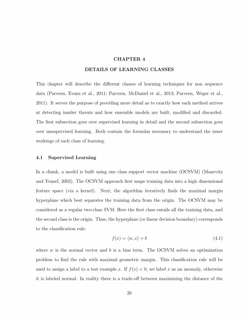
In a chunk, a model is built using one class support vector machine (OCSVM) (Manevitz

and Yousef, 2002). The OCSVM approach first maps training data into a high dimensional

feature space (via a kernel). Next, the algorithm iteratively finds the maximal margin

hyperplane which best separates the training data from the origin. The OCSVM may be

considered as a regular two-class SVM. Here the first class entails all the training data, and

the second class is the origin. Thus, the hyperplane (or linear decision boundary) corresponds

to the classification rule:

f(x) = 〈w, x〉+ b (4.1)

where w is the normal vector and b is a bias term. The OCSVM solves an optimization

problem to find the rule with maximal geometric margin. This classification rule will be

used to assign a label to a test example x. If f(x) < 0, we label x as an anomaly, otherwise

it is labeled normal. In reality there is a trade-off between maximizing the distance of the

26

27

E

A B

C D

E

A B

C D

E

A B

E D

C

A B

E D

E

A B

E D

Figure 4.1. A graph with a normative substructure (boxed) and anomalies (shaded)

hyperplane from the origin and the number of training data points contained in the region

separated from the origin by the hyperplane.

4.2 Unsupervised Learning

Algorithm 1 uses three varieties of graph based anomaly detection(GBAD) (Cook and Holder,

2007; Eberle and Holder, 2007; Cook and Holder, 2000; Yan and Han, 2002) to infer potential

anomalies using each model. GBAD is a graph-based approach to finding anomalies in data

by searching for three factors: modifications, insertions, and deletions of vertices and edges.

Each unique factor runs its own algorithm that finds a normative substructure and attempts

to find the substructures that are similar but not completely identical to the discovered

normative substructure. A normative substructure is a recurring subgraph of vertices and

edges that, when coalesced into a single vertex, most compresses the overall graph. The

rectangle in Figure 4.1 identifies an example of normative substructure for the depicted

graph.

Our implementation uses SUBDUE (Ketkar et al., 2005) to find normative substructures.

The best normative substructure can be characterized as the one with minimal description

length (MDL):

L(S,G) = DL(G | S) + DL(S) (4.2)

where G is the entire graph, S is the substructure being analyzed, DL(G | S) is the de-

scription length of G after being compressed by S, and DL(S) is the description length of

28

the substructure being analyzed. Description length DL(G) is the minimum number of bits

necessary to describe graph G (Eberle et al., 2011).

Insider threats appear as small percentage differences from the normative substructures.

This is because insider threats attempt to closely mimic legitimate system operations except

for small variations embodied by illegitimate behavior. We apply three different approaches

for identifying such anomalies, discussed below.

4.2.1 GBAD-MDL

Upon finding the best compressing normative substructure, GBAD-MDL searches for devia-

tions from that normative substructure in subsequent substructures. By analyzing substruc-

tures of the same size as the normative one, differences in the edges and vertices’ labels and

in the direction or endpoints of edges are identified. The most anomalous of these are those

substructures for which the fewest modifications are required to produce a substructure iso-

morphic to the normative one. In Figure 4.1, the shaded vertex labeled E is an anomaly

discovered by GBAD-MDL.

4.2.2 GBAD-P

In contrast, GBAD-P searches for insertions that, if deleted, yield the normative substruc-

ture. Insertions made to a graph are viewed as extensions of the normative substructure.

GBAD-P calculates the probability of each extension based on edge and vertex labels, and

therefore exploits label information to discover anomalies. The probability is given by

P (A=v) = P (A=v | A)P (A) (4.3)

where A represents an edge or vertex attribute and v represents its value. Probability

P (A=v | A) can be generated by a Gaussian distribution:

ρ(x) =1

σ√

2πexp

(−(x− µ)2

2σ2

)(4.4)

29

where µ is the mean and σ is the standard deviation. Higher values of ρ(x) correspond to

more anomalous substructures.

Using GBAD-P therefore ensures that malicious insider behavior that is reflected by

the actual data in the graph (rather than merely its structure) can be reliably identified

as anomalous by our algorithm. In Figure 4.1, the shaded vertex labeled C is an anomaly

discovered by GBAD-P.

4.2.3 GBAD-MPS

Finally, GBAD-MPS considers deletions that, if re-inserted, yield the normative substruc-

ture. To discover these, GBAD-MPS examines the parent structure. Changes in size and

orientation in the parent signify deletions amongst the subgraphs. The most anomalous

substructures are those with the smallest transformation cost required to make the parent

substructures identical. In Figure 4.1, the last substructure of A-B-C-D vertices is identified

as anomalous by GBAD-MPS because of the missing edge between B and D marked by the

shaded rectangle.

CHAPTER 5

EXPERIMENTS AND RESULTS

5.1 Dataset

We tested both of our algorithms on the 1998 Lincoln Laboratory Intrusion Detection

dataset (Kendall, 1998). This dataset consists of daily system logs containing all system

calls performed by all processes over a 7 week period. It was created using the Basic Secu-

rity Mode (BSM) auditing program. Each log consists of tokens that represent system calls

using the syntax exemplified in Figure 5.1.

The token arguments begin with a header line and end with a trailer line. The header

line reports the size of the token in bytes, a version number, the system call, and the date

and time of execution in milliseconds. The second line reports the full path name of the

executing process. The optional attribute line identifies the user and group of the owner,

the file system and node, and the device. The next line reports the number of arguments to

the system call, followed by the arguments themselves on the following line. The subject

line reports the audit ID, effective user and group IDs, real user and group IDs, process ID,

session ID, and terminal port and address, respectively. Finally, the return line reports the

outcome and return value of the system call.

Since many system calls are the result of automatic processes not initiated by any par-

ticular user, they are therefore not pertinent to the detection of insider threat. We limit our

attention to user-affiliated system calls. These include calls for exec, execve, utime, login,

logout, su, setegid, seteuid, setuid, rsh, rexecd, passwd, rexd, and ftp. All of these

correspond to logging in/out or file operations initiated by users, and are therefore relevant

to insider threat detection. Restricting our attention to such operations helps to reduce

30

31

header,129,2,execve(2),,Tue Jun 16 08:14:29 1998, +

518925003 msec

path/op/local/bin/tcsh

attribute,100755,root,other,8388613,79914,0

exec_args,1,

-tcsh

subject,2142,2142,rjm,2142,rjm,401,400,24

1 135.13.216.191

return,success,0

trailer,129

Figure 5.1. A sample system call record from the MIT Lincoln dataset

Time, userID, machineIP, command, arg, path, return

1 1:29669 6:1 8:1 21:1 32:1 36:0

Figure 5.2. Feature set extracted from Figure 5.1

extraneous noise in the dataset. Further, some tokens contain calls made by users from the

outside, via web servers, and are not pertinent to the detection of insider threats. There

are six such users in this data set and have been pulled out. Table 5.1 reports statistics

for the dataset after all irrelevant tokens have been filtered out and the attribute data in

Figure 5.3 has been extracted. Preprocessing extracted 62K tokens spanning 500K vertices.

These reflected the activity of all users over 9 weeks.

Figure 5.2 shows the features extracted from the output data in Figure 5.1 for our super-

vised approach and Figure 5.3 depicts the subgraph structure yielded for our unsupervised

approach.

The first number in Figure 5.2 is the classification of the token as either anomalous (-1) or

normal (1). The classification is used by 2-class SVM for training the model, but is unused

32

path

data

call

return

〈useraudit ID〉

IDterminalar

gs

procID

token〈path〉

〈data〉

〈call〉

〈returnvalue〉

〈terminal〉〈args〉〈proc ID〉

Figure 5.3. A token subgraph

(although required) for one class SVM. The rest of the line is a list of index-value pairs,

which are separated by a colon (:). The index represent the dimension for use by SVM,

and the value is the value of the token along that dimension. The value must be numeric.

The list must be ascending by index. Indices that are missing are assumed to have a value

of 0. Attributes which are categorical in nature (and can take the value of any one of N

categories) are represented by N dimensions. In Figure 5.2, 1:29669 means that the time

of day (in seconds) is 29669. 6:1 means that the user’s ID (which is categorical) is 2142,

8:1 means that the machine IP address (also categorical) is 135.13.216.191, 21:1 means that

the command (categorical) is execve, 32:1 means the path begins with /opt, and, and 36:0

means that the return value is 0. The mappings between the data values and the indices

were set internally by a configuration file.

All of these features are important for different reasons. The time of day could indicate

that the user is making system calls during normal business hours, or, alternatively, is logging

in late at night, which could be anomalous. The path could indicate the security level of

the system call being made for instance, a path beginning with /sbin could indicate use of

important system files, while a path like /bin/mail could indicate something more benign, like

sending mail. The user ID is important to distinguish events, what is anomalous for one user

may not be anomalous for another. A programmer that normally works from 9 A.M. to 5 P.M.

33

would not be expected to login at midnight, but a maintenance technician (who performs

maintenance on server equipment during off hours, at night), would. Frequent changes

in machine IP address or changes that are not frequent enough could indicate something

anomalous. Lastly, the system call itself could indicate an anomaly most users would be

expected to login and logout, but only administrators would be expected to invoke super

user privileges with a command such as su.

5.2 Experimental Setup

5.2.1 Supervised Learning

We used LIBSVM (Chang and Lin, 2011) to build our models and to generate predictions for

our test cases in our supervised approach. First, we will give an overview of our use of SVM

software, which is standard procedure and is well documented in LIBSVMs help files. We

chose to use the RBF (radial-based function) kernel for the SVM. It was chosen because it

gives good results for our data set. Parameters for the kernel (in the case of two-class SVM,

C and γ, and in the case of one-class SVM, ν and γ) were chosen so that the F1 measure was

maximized. We chose to use the F1 measure in this case (over other measures of accuracy)

because, for the classifier to do well according to this metric, it must minimize false positives

while also minimizing false negatives. Before training a model with our feature set, we used

LIBSVM to scale the input data to the range [0, 1]. This was done to ensure that dimensions

which takes on high values (like time) do not outweigh dimensions that take on low values

(such as dimensions which represent categorical variables). The parameters that were used

to scale the training data for the model are the same parameters that were used to scale that

model’s test data. Therefore, the model’s test data will be in the vicinity of the range [0, 1].

We conducted two experiments with the SVM. The first, as seen in Table 5.2, was de-

signed to compare one-class SVM with two-class SVM for the purposes of insider threat

34

Table 5.1. Dataset statistics after filtering and attribute extractionStatistic ValueNo of vertices 500,000No of tokens 62,000No of normative substructures 5No of users allDuration 9 weeks

detection, and the second, as seen in Table 5.3, was designed to compare a stream classifica-

tion approach with a more traditional approach to classification. We will begin by describing

our comparison of one-class and two-class SVM. For this experiment, we took the 7 weeks

of data, and randomly divided it into halves. We deemed the first half training data and

the other half testing data. We constructed a simple one-class and two-class model from the

training data and recorded the accuracy of the model in predicting the test data.

For the insider threat detection approach we use an ensemble-based approach that is

scored in real time. The ensemble maintains K models that use one-class SVM, each con-

structed from a single day and weighted according to the accuracy of the models previous

decisions. For each test token, the ensemble reports the majority vote of its models.

The stream approach outlined above is more practical for detecting insider threats be-

cause insider threats are stream in nature and occur in real time. A situation like that in the

first experiment above is not one that will occur in the real world. In the real world, insider

threats must be detected as they occur, not after months of data has piled in. Therefore, it

is reasonable to compare our updating stream ensemble with a simple one-class SVM model

constructed once and tested (but not updated) as a stream of new data becomes available,

see Table 5.3.

5.2.2 Unsupervised Learning

For our unsupervised approach (based on graph based anomaly detection), we needed to

accurately depict the effects of two variables. Those variables are K, the number of ensembles

35

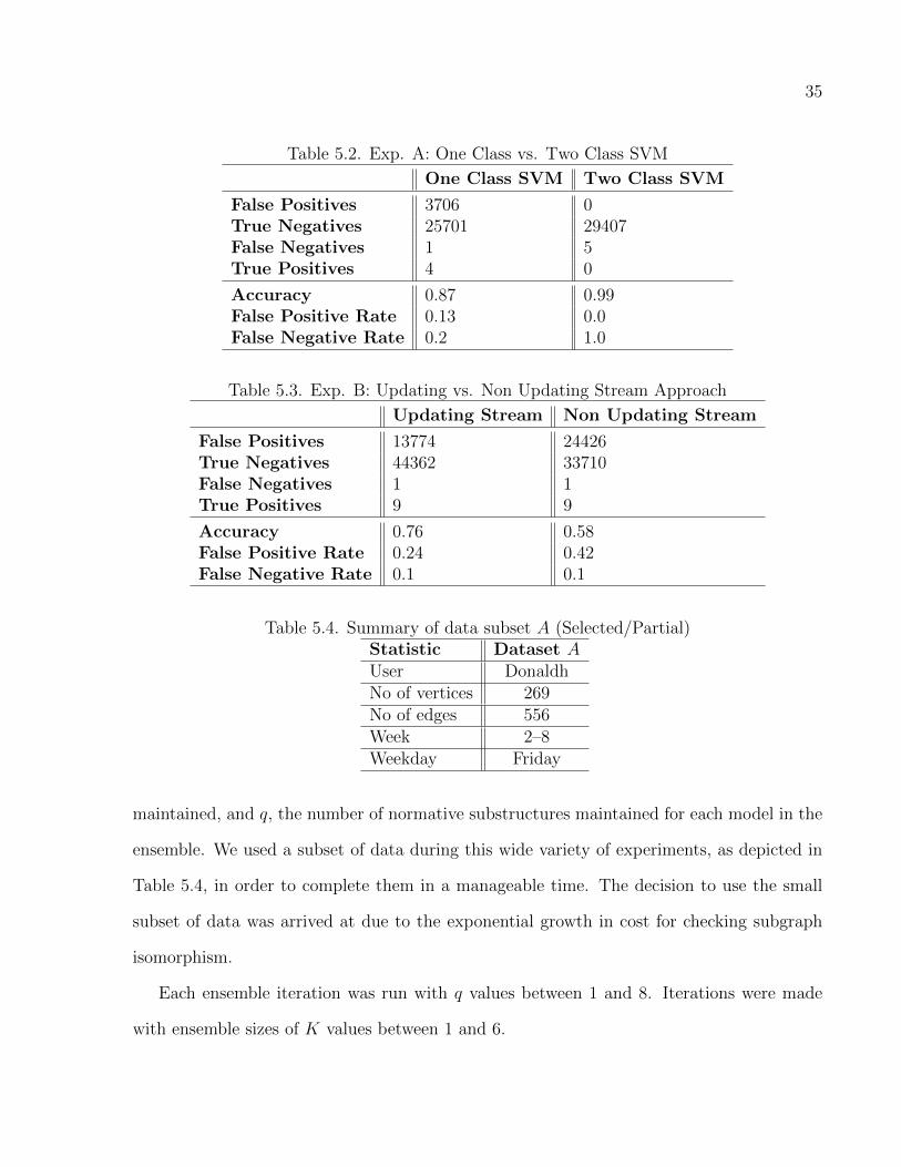
Table 5.2. Exp. A: One Class vs. Two Class SVM

One Class SVM Two Class SVM

False Positives 3706 0True Negatives 25701 29407False Negatives 1 5True Positives 4 0

Accuracy 0.87 0.99False Positive Rate 0.13 0.0False Negative Rate 0.2 1.0

Table 5.3. Exp. B: Updating vs. Non Updating Stream Approach

Updating Stream Non Updating Stream



Table 5.4. Summary of data subset A (Selected/Partial)Statistic Dataset AUser DonaldhNo of vertices 269No of edges 556Week 2–8Weekday Friday

maintained, and q, the number of normative substructures maintained for each model in the

ensemble. We used a subset of data during this wide variety of experiments, as depicted in

Table 5.4, in order to complete them in a manageable time. The decision to use the small

subset of data was arrived at due to the exponential growth in cost for checking subgraph

isomorphism.

Each ensemble iteration was run with q values between 1 and 8. Iterations were made

with ensemble sizes of K values between 1 and 6.

36

5.3 Results

5.3.1 Supervised Learning

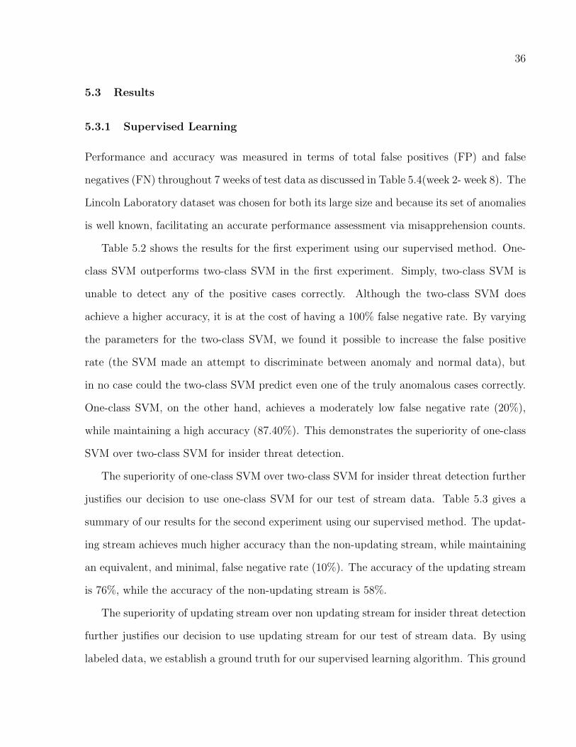
Performance and accuracy was measured in terms of total false positives (FP) and false

negatives (FN) throughout 7 weeks of test data as discussed in Table 5.4(week 2- week 8). The

Lincoln Laboratory dataset was chosen for both its large size and because its set of anomalies

is well known, facilitating an accurate performance assessment via misapprehension counts.

Table 5.2 shows the results for the first experiment using our supervised method. One-

class SVM outperforms two-class SVM in the first experiment. Simply, two-class SVM is

unable to detect any of the positive cases correctly. Although the two-class SVM does

achieve a higher accuracy, it is at the cost of having a 100% false negative rate. By varying

the parameters for the two-class SVM, we found it possible to increase the false positive

rate (the SVM made an attempt to discriminate between anomaly and normal data), but

in no case could the two-class SVM predict even one of the truly anomalous cases correctly.

One-class SVM, on the other hand, achieves a moderately low false negative rate (20%),

while maintaining a high accuracy (87.40%). This demonstrates the superiority of one-class

SVM over two-class SVM for insider threat detection.

The superiority of one-class SVM over two-class SVM for insider threat detection further

justifies our decision to use one-class SVM for our test of stream data. Table 5.3 gives a

summary of our results for the second experiment using our supervised method. The updat-

ing stream achieves much higher accuracy than the non-updating stream, while maintaining

an equivalent, and minimal, false negative rate (10%). The accuracy of the updating stream

is 76%, while the accuracy of the non-updating stream is 58%.

The superiority of updating stream over non updating stream for insider threat detection

further justifies our decision to use updating stream for our test of stream data. By using

labeled data, we establish a ground truth for our supervised learning algorithm. This ground

37

truth allows us to place higher weights on false negatives or false positives. By weighing one

more than the other, we punish a model more for producing that which we have increased the

weight for. When detecting insider threats it is more important that we do not miss a threat

(false negative) than identify a false threat (false positive). Therefor, we weigh false negative

more heavily–i.e. we add a FN cost. Figure 5.4 and figure 5.5 show the results of weighting

the false negatives more heavily than false positives with this established ground truth. This

is to say, that at a FN cost of 50, a false negative that is produced will count against a model

50 times more than a false positive will. Increasing the FN cost also increases the accuracy

of our OCSVM, updating stream approach. We can see that that increasing the FN cost up

to 30 only increases the total cost without affecting the accuracy, but after this, the accuracy

climbs and the total cost comes down. Total cost, as calculated by equation 5.1, represents

the total number of false positives and false negative after they have been modified by the

increase FN Cost. We see this trend peak at a FN cost of 80 where accuracy reaches nearly

56% and the total cost is at a low of 25229.

TotalCost = TotalFalsePositives + (TotalFalseNegatives ∗ FNCost) (5.1)

The false negatives are weighted by cost more heavily than false positives because it is

more important to catch all insider threats. False positives are acceptable in some cases,

but an insider threat detection system is useless if it does not catch all positive instances

of insider threat activity. This is why models who fail to catch positive cases and produce

these false negatives are punished, in our best case result, 80 times more heavily than those

who produce false positives.

Table 5.5 reinforces our decision to include FN cost during model elimination that heav-

ily punishes models who produce false negatives over those that produce false positives.

Including FN cost increases the accuracy of the ensemble and provides a better F2 Measure.

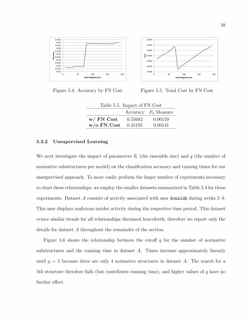
38

0.552

0.5525

0.553

0.5535

0.554

0.5545

0.555

0.5555

0.556

0.5565

0.557

0.5575

0 50 100 150 200

Acc

ura

cy

False Negative Cost

Figure 5.4. Accuracy by FN Cost

25200

25250

25300

25350

25400

25450

25500

0 50 100 150 200

Co

st

False Negative Cost

Figure 5.5. Total Cost by FN Cost

Table 5.5. Impact of FN Cost

Accuracy F2 Measure

w/ FN Cost 0.55682 0.00159w/o FN Cost 0.45195 0.00141

5.3.2 Unsupervised Learning

We next investigate the impact of parameters K (the ensemble size) and q (the number of

normative substructures per model) on the classification accuracy and running times for our

unsupervised approach. To more easily perform the larger number of experiments necessary

to chart these relationships, we employ the smaller datasets summarized in Table 5.4 for these

experiments. Dataset A consists of activity associated with user donaldh during weeks 2–8.

This user displays malicious insider activity during the respective time period. This dataset

evince similar trends for all relationships discussed henceforth; therefore we report only the

details for dataset A throughout the remainder of the section.

Figure 5.6 shows the relationship between the cutoff q for the number of normative

substructures and the running time in dataset A. Times increase approximately linearly

until q = 5 because there are only 4 normative structures in dataset A. The search for a

5th structure therefore fails (but contributes running time), and higher values of q have no

further effect.

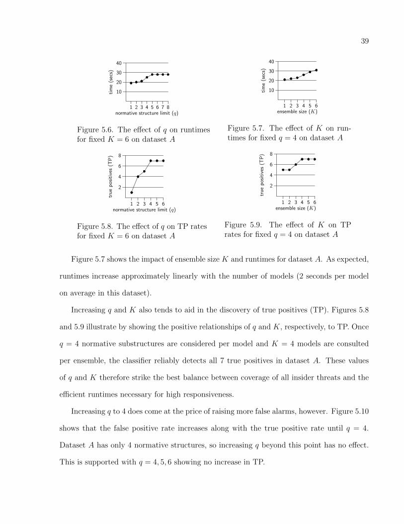
39

1 2 3 4 5 6 7 8

10

20

30

40

normative structure limit (q)ti

me

(sec

s)

Figure 5.6. The effect of q on runtimesfor fixed K = 6 on dataset A

1 2 3 4 5 6

10

20

30

40

ensemble size (K)

tim

e(s

ecs)

Figure 5.7. The effect of K on run-times for fixed q = 4 on dataset A

1 2 3 4 5 6

2

4

6

8

normative structure limit (q)

tru

ep

osit

ives

(TP

)

Figure 5.8. The effect of q on TP ratesfor fixed K = 6 on dataset A

1 2 3 4 5 6

2

4

6

8

ensemble size (K)

tru

ep

osit

ives

(TP

)

Figure 5.9. The effect of K on TPrates for fixed q = 4 on dataset A

Figure 5.7 shows the impact of ensemble size K and runtimes for dataset A. As expected,

runtimes increase approximately linearly with the number of models (2 seconds per model

on average in this dataset).

Increasing q and K also tends to aid in the discovery of true positives (TP). Figures 5.8

and 5.9 illustrate by showing the positive relationships of q and K, respectively, to TP. Once

q = 4 normative substructures are considered per model and K = 4 models are consulted

per ensemble, the classifier reliably detects all 7 true positives in dataset A. These values

of q and K therefore strike the best balance between coverage of all insider threats and the

efficient runtimes necessary for high responsiveness.

Increasing q to 4 does come at the price of raising more false alarms, however. Figure 5.10

shows that the false positive rate increases along with the true positive rate until q = 4.

Dataset A has only 4 normative structures, so increasing q beyond this point has no effect.

This is supported with q = 4, 5, 6 showing no increase in TP.

40

1 2 3 4 5 6

50

100

150

normative structure limit (q)

fals

ep

osit

ives

(FP

)

Figure 5.10. The effect of q on FP rates for fixed K = 6 on dataset A

Table 5.6. Impact of fading factor λ (weighted voting)

K = 2 K = 3 K = 4

λ=1 λ=0.9 λ=1 λ=0.9 λ=1 λ=0.9

TP 10 10 10 10 14 14FP 79 79 85 85 124 85TN 96 96 90 90 51 90FN 4 4 4 4 0 0

Table 5.6 considers the impact of weighted versus unweighted majority voting on the

classification accuracy. The unweighted columns are those for λ = 1, and the weighted

columns use fading factor λ = 0.9. The dataset consists of all tokens associated with user

ID 2143. Weighted majority voting has no effect in these experiments except when K = 4,

where it reduces the FP rate from 124 (unweighted) to 85 (weighted) and increases the TN

rate from 51 (unweighted) to 90 (weighted). However, since these results can be obtained for

K = 3 without weighted voting, we conclude that weighted voting merely serves to mitigate

a poor choice of K; weighted voting has little or no impact when K is chosen wisely.

Table 5.7 gives a summary of our results comparing our supervised and unsupervised

learning approaches. For example, on dataset A the supervised learning achieves much

higher accuracy (71%) than the unsupervised learning (56%), while maintaining lower false

positive rate (31%) and false negative rate (0%). On the other hand, unsupervised learning

achieves 56% accuracy, 54% false positive rate and 42% false negative rate.

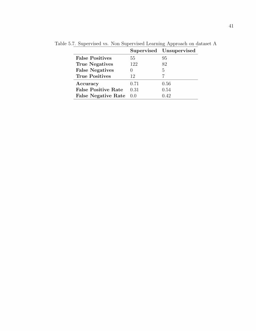
41

Table 5.7. Supervised vs. Non Supervised Learning Approach on dataset A

Supervised Unsupervised



CHAPTER 6

INSIDER THREAT DETECTION FOR SEQUENCE DATA

A sequence is an ordered list of objects (or events). Sequence contains members (also called

elements, or terms). In a set, element order does not matter. On the other hand, in a

sequence order matters, and hence, exactly the same elements can appear multiple times at

different positions in the sequence (Qumruzzaman et al., 2013). For example, (U,T,D) is a

sequence of letters with the letter ’U’ first and ’D’ last. This sequence differs from (D,T,U).

The sequence (U,T,D,A,L,L,A,S), which contains the alphabet ’A’ at two different positions,

is a valid sequence. In the Figure 6.1 illustrates some sequence of movement pattern of

a user. First row represents a particular user’s one movement pattern sequence: student

center, office, and ml. In this sequence, the user was first at student center and ml (media

Lab) at last (Eagle and (Sandy) Pentland, 2006).

As the length of the sequence is defined as the number of ordered elements, sequence data

can be finite or infinite in length. Infinite sequences are known as stream sequence data.

Insider threat detection related sequence data is stream based in nature. Sequence data

may be gathered over time, maybe even years. In this case, we assume a continuous data

stream will be converted into a number of chunks. For example, each chunk may represent

a week and contain the sequence data which arrived during that time period.

Figure 6.2 demonstrates how the classifier decision boundary changes over time (from one

chunk to next chunk). Data points are associated with two classes (normal and anomalous).

In particular, a user command or a sub-sequence of commands may form a pattern/phrase

which will be called here as data point. Non repetitive pattern/phrase for a user may form

anomaly. There are three contiguous data chunks as shown in the Figure 6.2. The dark

42

43

Figure 6.1. Example of Sequence Data related to Movement Pattern

straight line represents the decision boundary of its own chunk, whereas the dotted straight

line represents the decision boundary of previous chunk. If there were no concept drift in the

data stream, the decision boundary would be the same for both the current chunk and its

previous chunk (the dotted and straight line). White dots represent the normal data (True

Negative), blue dots represent anomaly data (True Positive), and striped dots represent the

instances victim of concept drift.

We show the two different cases in the Figure 6.2 are as follows.

Case 1: the decision boundary of the second chunk moves upwards compared to that of

the first chunk. As a result, more normal data will be classified as anomalous by the decision

boundary of the first chunk, thus FP will go up. Recall that a test point having true benign

(normal) category classified as an anomalous by a classifier is known as a FP.

Case 2: the decision boundary of the third chunk moves downwards compared to that of

the first chunk. So, more anomalous data will be classified as normal data by the decision

boundary of the first chunk, thus FN will go up. Recall that a test point having true malicious

category classified as benign by a classifier is known as a FN.

In the more general case, the decision boundary of the current chunk can vary, which

causes the decision boundary of the previous chunk to mis-classify both normal and anoma-

lous data. Therefore, both FP and FN may go up at the same time.

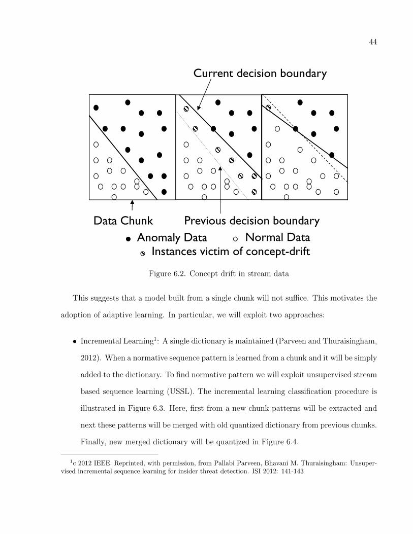
44

Concept-Drift

Anomaly Data Normal Data

Data Chunk

Current decision boundary

Previous decision boundary

Instances victim of concept-drift

Figure 6.2. Concept drift in stream data

This suggests that a model built from a single chunk will not suffice. This motivates the

adoption of adaptive learning. In particular, we will exploit two approaches:

• Incremental Learning1: A single dictionary is maintained (Parveen and Thuraisingham,

2012). When a normative sequence pattern is learned from a chunk and it will be simply

added to the dictionary. To find normative pattern we will exploit unsupervised stream

based sequence learning (USSL). The incremental learning classification procedure is

illustrated in Figure 6.3. Here, first from a new chunk patterns will be extracted and

next these patterns will be merged with old quantized dictionary from previous chunks.

Finally, new merged dictionary will be quantized in Figure 6.4.

1c 2012 IEEE. Reprinted, with permission, from Pallabi Parveen, Bhavani M. Thuraisingham: Unsuper-vised incremental sequence learning for insider threat detection. ISI 2012: 141-143

45

• Ensemble Learning2: A number of dictionaries are maintained (Parveen, McDaniel

et al., 2012). In the ensemble we maintain K models. For each model, we maintain a

single dictionary. Our ensemble approach, which classifies data using an evolving set

of K models. The ensemble classification procedure is illustrated in Figure 6.5. Recall

that we use unsupervised stream based sequence learning (USSL) to train models from

an individual chunk. USSL identifies the normative patterns in the chunk and stores

it in a quantized dictionary.

In the literature (Masud, Chen, Gao, Khan, Aggarwal et al., 2010; Masud et al., 2011a;

Masud, Gao et al., 2008) it shows that ensemble based learning is more effective than incre-

mental learning. Here, we will focus on ensemble based learning.

To identify an anomaly, a test point will be compared against each model of the ensemble.

Recall that a model will declare the test data as an anomalous based on how much the test

differs from the model’s normative patterns. Once all models cast their vote, we will apply

majority voting to make the final decision as to whether the test point is an anomalous or

not (as shown in Figure 3.2).

6.1 Model Update

We always keep an ensemble of fixed size models (K in that case). Hence, when a new chunk

is processed, we already have K models in the ensemble and the K + 1st model will be

created from the current chunk. We need to update ensemble by replacing a victim model

with this new model. Victim selection can be done in a number of ways. One approach

is to calculate the prediction error of each model on the most recent chunk relative to the

majority vote. Here, we assume ground truth on the most recent chunk is not available. If

2c 2012 IEEE. Reprinted, with permission, from Pallabi Parveen, Nate McDaniel, Varun S. Hariharan,Bhavani M. Thuraisingham, Latifur Khan: Unsupervised Ensemble Based Learning for Insider Threat De-tection. SocialCom/PASSAT 2012: 718-727

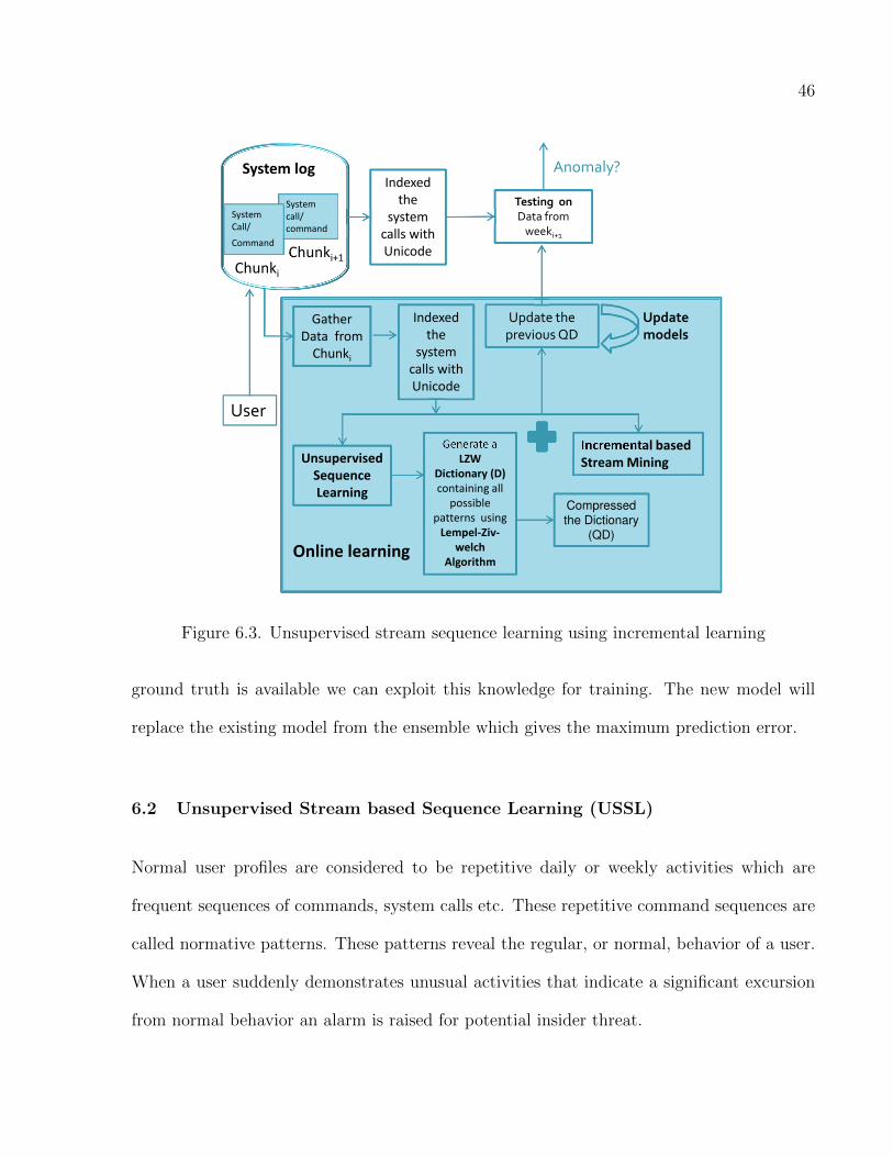
46

Indexed

the

system

calls with

Unicode

Anomaly?

j

System

call/

command

System

Call/

Command Chunki+1

Chunki

System log

Testing on

Data from

weeki+1

Gather

Data from

Chunki

Indexed

the

system

calls with

Unicode

Unsupervised

Sequence

LearningCompressed

the Dictionary

(QD)

Generate a

LZW

Dictionary (D)

containing all

possible

patterns using

Lempel-Ziv-

welch

Algorithm

Incremental based

Stream Mining

Update the previous QD

Update

models

Online learning

User

Figure 6.3. Unsupervised stream sequence learning using incremental learning

ground truth is available we can exploit this knowledge for training. The new model will

replace the existing model from the ensemble which gives the maximum prediction error.

6.2 Unsupervised Stream based Sequence Learning (USSL)

Normal user profiles are considered to be repetitive daily or weekly activities which are

frequent sequences of commands, system calls etc. These repetitive command sequences are

called normative patterns. These patterns reveal the regular, or normal, behavior of a user.

When a user suddenly demonstrates unusual activities that indicate a significant excursion

from normal behavior an alarm is raised for potential insider threat.

47

LZW Dictionary

OLD Quantized Dictionary (OQD)

Session 1Session 2

Session n

LZW

LZW

LZW

compression

LZWDictionary

LZW

New Quantized Dictionary (NQD)

compression

Session 1Session 2

Session n

LZW

LZW

LZW

Figure 6.4. Details block diagram of incremental learning

So, in order to identify an insider threats, first we need to find normal user behavior. For

that we need to collect sequences of commands and find the potential normative patterns

observed within these command sequences in an unsupervised fashion. This unsupervised

approach also needs to identify normal user behavior in a single pass. One major challenge

with these repetitive sequences is their variability in length. To combat this problem, we need

to generate a dictionary which will contain any combination of possible normative patterns

existing in the gathered data stream. Potential variations that could emerge within the data

include the commencement of new events, the omission or modification of existing events, or

the reordering of events in the sequence. Eg., liftliftliftliftliftcomcomecomecomecome-come,

is a sequence of commands represented by the alphabets given in a data stream. . We will

consider all patterns li,if,ft,tl, lif, ift, ftl, lift, iftl etc., as our possible normative patterns.

However, the huge size of the dictionary presents another significant challenge.

We have addressed the above two challenges in the following ways. First, we extract possi-

ble patterns from the current data chunk using single pass algorithm (e.g., LZW, Lempel-Ziv-

48

Indexed the

system calls with Unicode

Anomaly?

j

System call/command

System Call/

Command Chunki+1

Chunki

System log

Testing on Data from

weeki+1

Online learning

Generate a LZW Dictionary

Gather Data from

Chunki

Indexed 0the

system calls with Unicode

Unsupervised Sequence Learning

Compressed the Dictionary

(QD)

LZW Dictionary (D) containing

all possible patterns using

Lempel-Ziv-welch

Algorithm

Ensemble based Stream Mining

Ensemble of Models

Update models

Figure 6.5. Ensemble based unsupervised stream sequence learning

LZW

DictionaryQuantized

Dictionary

(QD)

Session 1Session 2

Session n

LZW

LZW

LZW

compression

Figure 6.6. Unsupervised Stream based Sequence Learning(USSL)from a chunk in Ensemblebased case

49

Welch algorithm (Ziv and Lempel, 1977)) to prepare a dictionary. We called it LZW dic-

tionary. LZW dictionary has a set of patterns and their corresponding weights according

to

wi =fi∑ni=1 fi

(6.1)

where wi is the weight of a particular pattern pi in the current chunk, fi is the number

of times the pattern pi appears in the current chunk and n is the total number of distinct

patterns found in that chunk.

Next, we compress the dictionary by keeping only the longest, frequent unique patterns

according to their associated weight and length, while discarding other subsumed patterns.

This technique is called compression method (CM) and the new dictionary is a Quantized

dictionary (QD). The Quantized dictionary has a set of patterns and their corresponding

weights. Here, we use edit distance to find the longest pattern. Edit distance is a measure of

similarity between pairs of strings (Borges et al., 2011; Vladimir, 1966). It is the minimum

number of actions required to transfer one string to another, where an action can be substi-

tution, addition or deletion of a character into the string. As in case of the earlier example

mentioned, the best normative pattern in the quantized dictionary would be lift, come etc.

This process is a lossy compression, but is sufficient enough to extract the meaningful

normative patterns. The reason behind this is the patterns that we extract are the superset

of the subsumed patterns. Moreover, as frequency is another control parameter in our

experiment, the patterns which do not appear often cannot be regular user patterns.

Data relevant to insider threat is typically accumulated over many years of organization

and system operations, and is therefore best characterized as an unbounded data stream.

As our data is a continuous stream of data, we use ensemble based learning to continuously

update our compressed dictionary. This continuous data stream is partitioned into a sequence

of discrete chunks. For example, each chunk might be comprised of a day or weeks worth of

data and may contain several user sessions. We generate our Quantized dictionary (QD) and

50

Figure 6.7. Quantization of dictionary

their associated weight from each chunk. Weight is measured as the normalized frequency

of a pattern within that chunk.

When a new chunk arrives we generate a new Quantized dictionary (QD) model and

update the ensemble as mentioned earlier. Figure 6.6 shows the flow diagram of our dynamic,

Ensemble based, Unsupervised Stream Sequence Learning method.

Algorithm 4 shows the basic building block for updating the Ensemble. Algorithm 4

takes the most recent data chunk S, ensemble E and test chunk T . Lines 3 to 4 generate a

new Quantized Dictionary model from the most recent chunk S and temporarily add it to

the ensemble E. Lines 5 to 9 test chunk T for anomalies for each model in the ensemble.

Lines 13 to 24 find and label the anomalous patterns in test Chunk T according to the

majority voting of the models in the ensemble. Finally, line 29 updates the ensemble by

discarding the model with lowest accuracy. An arbitrary model is discarded in the case of

multiple models having the same low performance.

51

6.2.1 Construct the LZW dictionary by selecting the patterns in the data

stream

At the beginning, we consider that our data is not annotated (i.e., unsupervised). In other

words, we don’t know the possible sequence of future operations by the user. So, we use

LZW algorithm (Ziv and Lempel, 1977) to extract the possible sequences that we can add to

our dictionary. These can also be commands like liftliftliftliftliftcomcomecomecomecomecome,

where each unique letter represents a unique system call or command. We have used Unicode

to index each command. E.g., ls, cp, find are indexed as l, c, and f. The possible patterns or

sequences are added to our dictionary would be li, if,ft,tl, lif,ift, ftl, lift, iftl, ftli, tc, co, om,

mc,com, come and so on. When the sequence li is seen in the data stream for the second

time, in order to avoid repetition it will not be included in the LZW dictionary. Instead,

we increase the frequency by 1 and extend the pattern by concatenating it with the next

character in the data stream, thus turning up a new pattern lif. We will continue the process

until we reach the end of the current chunk. Figure 6.7 demonstrates how we generate an

LZW dictionary from the data stream.

6.2.2 Constructing the Quantized Dictionary

Once we have our LZW dictionary, we keep the longest and most frequent patterns and dis-

card all their subsumed patterns. Algorithm 5 shows step by step how a quantized dictionary

is generated from LZW dictionary. Inputs of this algorithm are as follows: LZW dictionary

D which contains a set of patterns P and their associated weight W . Line 5 picks a pattern

(e.g., li). Lines 7 to 9 find all the closest patterns that are 1 edit distance away. Lines 13

to 16 keep the pattern which has the highest weight multiplied by its length and discard the

other patterns. We repeat the steps (line 5 to 16) until we find the longest, frequent pattern

(lift). After that, we start with a totally different pattern (co) and repeat the steps until we

have explored all the patterns in the dictionary. Finally, we end up with a more compact

52

Algorithm 4 Update the Ensemble

1: Input: E (ensemble), T (test chunk), S (chunk)2: Output: E ′ (updated ensemble)3: M ′ ← NewModel(S)4: E ′ ← E ∪ {M ′}5: for each model M in ensemble E do6: AM ← T7: for each pattern p in M do8: if EditDistance(x, p) ≤ α = 1

3of length then

9: AM = AM − x10: end if11: end for12: end for13: for each candidate a in

⋃M∈E′ AM do

14: if round(WeightedAverage(E ′, a)) = 1 then15: A← A ∪ {a}16: for each model M in ensemble E ′ do17: if a ∈ AM then18: cM ← cM + 119: end if20: end for21: else22: for each model M in ensemble E ′ do23: if a 6∈ AM then24: cM ← cM + 125: end if26: end for27: end if28: end for29: E ′ ← E ′ − {choose(arg minM(cM))}

53

Algorithm 5 Quantized Dictionary

1: Input: D = {Pattern,Weight} (LZW Dictionary)2: Output: QD (Quantized Dictionary)3: V isited← 04: while D 6= 0 do5: X ← Dj | j 6∈ V isited,Dj ∈ D6: V isited← V isited ∪ j7: for each pattern i in D do8: if EditDistance(X,Di) = 1 then9: P ← P ∪ i

10: end if11: end for12: D ← D −X13: if P 6= 0 then14: X ← choose(arg maxi(wi × li)) | li = Length(Pi), wi = Weight(Pi), Pi ∈ P15: QD ← QD ∪X16: D ← D − P17: end if18: X ← Dj | j 6∈ V isited,Dj ∈ D19: V isited← V isited ∪ j20: end while

dictionary which will contain many meaningful and useful sequences. We call this dictionary

our quantized dictionary. Figure 6.7 demonstrates how we generate a quantized dictionary

from the LZW dictionary.

Once, we identify different patterns lift, come, etc., any pattern with X%(≥ %30 in our

implementation) deviation from all these patterns would be considered as anomaly. Here,

we will use edit distance to identify the deviation.

6.3 Anomaly Detection (Testing)

Given a quantized dictionary, we need to find out the sequences in the data stream which may

raise a potential threat. To formulate the problem, given the data stream S and Ensemble

E where E = QD1, QD2, QD3, ... and QDi = qdi1, qdi2, ... , any pattern in the data stream

is considered as an anomaly if it deviates from all the patterns qdij in E by more than

54

Table 6.1. Time Complexity of Quantization Dictionary ConstructionDescription Time ComplexityPair of Patterns O(n2 ×K2)u number of user O(u× n2 ×K2)

X%(say > 30%). In order to find the anomalies, we need to first find the matching patterns

and delete those from the stream S. In particular, we find the pattern from the data stream

S that is an exact match or α edit distance away from any pattern, qdij in E. This pattern

will be considered as matching pattern. α can be half, one-third or one-fourth of the length

of that particular pattern in qdij. Next, remaining patterns in the stream will be considered

as anomalies.

In order to identify the non matching patterns in the data stream S, we compute a

distance matrix L which contains the edit distance between each pattern, qdij in E and the

data stream S. If we have a perfect match, i.e., edit distance 0 between a pattern qdij and

S, we can move backwards exactly the length of qdij in order to find the starting point of

that pattern in S and then delete it from the data stream. On the other hand, if there is an

error in the match which is greater than 0 but less than α, in order to find the starting point

of that pattern in the data stream, we need to traverse either left, or diagonal or up within

the matrix according to which one among the mentioned value (L[i,j-1], L[i-1,j-1], L[i-1,j])

gives the minimum respectively. Finally, once we find the starting point, we can delete that

pattern from the data stream. The remaining patterns in the data stream will be considered

as anomalous.

6.4 Complexity Analysis

Here, we will report time complexity of quantized dictionary construction. In order to

calculate edit distance between two patterns of length K (in worst case maximum length

would be K), our worst case time complexity would be O(K2).

55

Suppose we have n patterns in our LZW dictionary. We have to construct quantized

dictionary from this LZW dictionary. In order to do this, we need to find patterns in LZW

dictionary which have 1 edit distance from a particular pattern (say p). We have to calculate

edit distance between all the patterns and the pattern p. Recall that time complexity to

find edit distance between two patterns is O(K2). Since there are total n number of distinct

patterns, total time complexity between p and the rest of patterns is O(n×K2). Note that p

is one of the member of n patters. Therefore, total time complexity between pair of patterns

is O(n2 × K2). This is valid for a single user. If there is u of distinct users, total time

complexity across u user is O(u× n2 ×K2) (see Table 6.1)

CHAPTER 7

EXPERIMENTS AND RESULTS FOR SEQUENCE DATA

Here, first we will present sequence dataset that we used for experiment. Second, we present

how we inject concept drift in the dataset. Finally, we present results showing anomaly

detection rate in the presence of concept drift1.

7.1 Dataset

The data sets used for training and testing have been created from Trace Files got from

the University of Calgary project (Greenberg, 1988). As a part of that, 168 trace files were

collected from 168 different users of Unix csh. There were 4 groups of people, namely novice-

programmers, experienced-programmers, computer-scientists, non-programmers. The model

that we have tried to construct is that of a novice-programmer who has been gaining ex-

perience over the weeks and is gradually using more and more command sequences similar

to that of an experienced user. These gradual normal behavior changes will be known here

as concept-drift. Anomaly detection in the presence of concept drift is difficult to achieve.

Hence, our scenario is more realistic. This is a slow process that takes place over several

weeks.

The Calgary dataset (Greenberg, 1988) as described above was modified by Maxion et

al. (Maxion, 2003) for masquerade detection. Here we followed the same guidelines to inject

masquerades commands. From the given list of users, those users who have executed more

than 2400 commands (that did not result in an error) were filtered out to form the valid-user

1c 2012 IEEE. Reprinted, with permission, from Pallabi Parveen, Nate McDaniel, Varun S. Hariharan,Bhavani M. Thuraisingham, Latifur Khan: Unsupervised Ensemble Based Learning for Insider Threat De-tection. SocialCom/PASSAT 2012: 718-727

56

57

Table 7.1. Description of DatasetDescription Number# of valid users 37# of invalid users 131# of valid commands per user 2400# of anomalous commands in testing chunks 300

pool. This list had 37 users. The remaining users were part of the invalid-user pool. Out

of the list of invalid-users, 25 of them were chosen at random and a block of one hundred

commands from the commands that they had executed were extracted and put together to

form a list of 2500 (25 * 100) commands. The 2500 commands were brought together as 250

blocks of 10 commands each. Out of these 250 blocks, 30 blocks were chosen at random as

the list of masquerade commands (300 commands). For each user in the valid users list, the

total number of commands was truncated to 2400. These 2400 commands were split into 8

chunks of 300 commands each. The first chunk was kept aside as the training chunk (this

contains no masquerade data). The other 7 chunks are the testing chunks. In the testing

chunks, a number of masquerade data blocks (each block comprising of 10 commands) were

inserted at random positions. As a result, for each user, we have one training chunk with

300 commands (no masquerade data) and seven testing chunks which together have 2100

non-anomalous commands and 300 masquerade commands (see Table 7.1 and Figure 7.1).

7.2 Concept Drift in the training set

Here, we present a framework for concept drift with the goal of introducing artificial drift

into data generators. First, we generate a number of chunks having normal and anomalous

sequences as described above. Note that the above process does not take into account

concept drift. Next, we take sequences of each chunk as input and generate a new sequence

with a particular drift for that chunk. New sequences will have concept drift property. The

framework processes each training example of user commands once and only once to produce

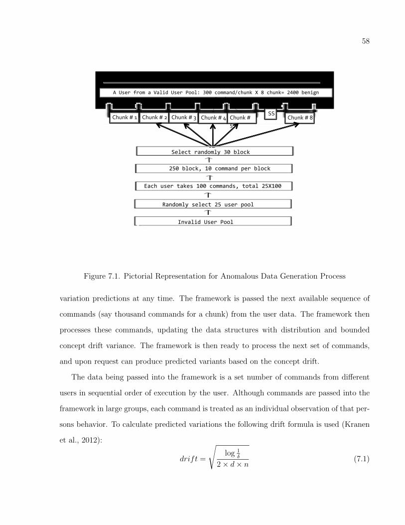
58

Chunk # 1 Chunk # 2 Chunk # 3 Chunk # 4 Chunk # 5

SSChunk # 8

Select randomly 30 block

A User from a Valid User Pool: 300 command/chunk X 8 chunk= 2400 benign command

Invalid User Pool

Randomly select 25 user pool

Each user takes 100 commands, total 25X100

250 block, 10 command per block

Figure 7.1. Pictorial Representation for Anomalous Data Generation Process

variation predictions at any time. The framework is passed the next available sequence of

commands (say thousand commands for a chunk) from the user data. The framework then

processes these commands, updating the data structures with distribution and bounded

concept drift variance. The framework is then ready to process the next set of commands,

and upon request can produce predicted variants based on the concept drift.

The data being passed into the framework is a set number of commands from different

users in sequential order of execution by the user. Although commands are passed into the

framework in large groups, each command is treated as an individual observation of that per-

sons behavior. To calculate predicted variations the following drift formula is used (Kranen

et al., 2012):

drift =

√log 1

δ

2× d× n(7.1)

59

where δ is the variation constant, d is the current distribution of the command over the

current number of individual observations, and n is the number of current observations

made. A good value for the variation constant is 1 ∗ 10−5. The variation constant shares

an inverse relation to the overall drift values. The expected range in distribution among

produced variations is calculated by adding and subtracting the calculated drift from the

current distribution.

Upon the processing of a sample of user commands, predicted variations can be produced

by the framework upon request. The request can be made of any designated size and the

concept drift will provide new distributions that fall within the range of the calculated drift

for a set of commands of this size. The produced set of commands or new ones can be used

to update the concept drift and provide for a constantly evolving command distribution that

represents an individual. Sudden changes that do not fit within a calculated concept drift

can be flagged as suspicious and therefore, possibly representative of an insider threat.

Algorithm 6 shows how the distribution is calculated for a set of commands and how

the predicted variation is produced. As an example we take ten commands, instead of one

thousand per chunk, such that we have [C1, C2, C1, C2, C3, C1, C4, C5, C1, C1]. The distribu-

tions will be [C1 = .5, C2 = .2, C3 = .1, C4 = .1, C5 = .1]. With a value of δ = 1 ∗ 10−5 the

Predicted Variance for each command comes out as

C1 =

√log 1

1∗10−5

2 ∗ .5 ∗ 10≈ .7071#ofoccurance (7.2)

We divide by the number of observation occurrences, in this case 10, because we want the

concept drift per occurrence, not just for a sample of 10. Our predicted variation (PV)

values are [C1 ≈ .07071, C2 ≈ .11180, C3 ≈ .15811, C4 ≈ .15811, C5 ≈ .15811]. The ad-

justed Min/Max Drift comes out to be [C1 = .42929/.57071, C2 = .08820/.31180, C3 =

0/.25811, C4 = 0/.25811, C5 = 0/.25811].

From these drift values we can produce a requested predicted variation for another 10,

or any number of, user command values. We look at the original sequence and assemble

60

Algorithm 6 Concept Drift in Sequence Stream

1: Input: F (file), (size of PV)2: Output: PV , (prediction variation)3: for each command C ∈ F do4: DC ← distribution(C )5: VC ← variation(DC)6: MaxDriftC ← DC + VC7: MinDriftC ← DC − VC8: end for9: PV ← newPredictedV ariation()

10: for each command C ∈ F do11: if DC < MinDriftC then12: PV ← PV ∪ C13: else14: if DC + 1 < MaxDriftC then15: flipCoin(PV ← PV ∪ C)16: else17: discard(C)18: end if19: end if20: end for

at least the minimum drift value worth of commands in the variation. In this example the

first value is C1 with a minimum of .42929 distribution. So we add it, bringing its current

distribution to 1/10 or .1. This is the case for the first 3 values resulting in [C1, C2, C1]. The

fourth value is C2 who has met its minimum distribution drift. Adding it will not go over the

maximum distribution so it is either randomly added or not. The new predicted variation

could look like [C1, C2, C1, C2, C1, C1, C1, C2, C3, C4] or [C1, C2, C1, C3, C1, C4, C1, C5, C3, C1]

of which both have command distributions similar to the original that fall within the new

variance bounds.

We compare our approach, USSL, with a supervised method modified from the baseline

approach suggested by Maxion (Maxion, 2003), which uses Naive Bayes’ classifier (NB). The

modified version compared in this dissertation is more incremental in its model training,

and thus will be referred to as NB-INC. All instances of both algorithms were tested using

61

8 chunks of data. At every test chunk the NB-INC method uses all previously seen chunks

to build the model and train for the current test chunk. For test chunk 3, NB builds the

classification model and trains on chunks 1 and 2. For test chunk 5 NB builds a model and

collectively trains on chunks 1 through 4.

These USSL statistics are gathered in a ”Grow as you Go” (GG) fashion. This is to say

that, as the ensemble size being used grows larger the amount of test chunks to go through

decreases. For an ensemble size of 1, models are built from chunk 1 and chunks 2 through 8

are considered testing chunks. For an ensemble size of 3, chunks 4 through 8 are considered

to be testing chunks. Every new chunk, starting at 4 in this case, is used to update the

models in each ensemble after a majority vote is reached and the test data is classified as

an anomaly or not. To clarify, in the example of ensemble size of 3 after the new model is

built, all models vote on the possible anomaly and contribute to deciding which model is

considered the least accurate and thus discarded. However, only models that have survived

an elimination round (i.e. deemed not to be least accurate at least once) are used to measure

the FP, TP, FN, and TN for an ensemble. In particular, at chunk 4, the ensemble has 3

models from chunk 1, 2, and 3. From chunk 4, new model is built. During elimination round,

chunk 3 is eliminated based on accuracy. In other words, at chunk 4, ensemble will have

models created from chunks 1, 2, and 4 but not 3.

The model updating process makes use of compression and model replacement. After

models are updated the least accurate one is discarded to maintain the highest accuracy

and maintain the status quo, since a new model is created before every update and anomaly

classification step. There are other ways of updating models and selecting chunks for testing

during the classification process not explored in this dissertation. For this purpose, the

limited USSL method used for the shown results will be referred to as USSL-GG.

62

7.3 Result

We have compared the NB and USSL-GG algorithms on the basis of true positive rate(TPR),

false positive rate(FPR), execution time, accuracy, F1 measure, and F2 measure. TPR and

FPR as measured by

TPR =true positives

true positives+ false negatives(7.3)

FPR =false positives

false positives+ true negatives(7.4)

are the rates at which actual insider threats are correctly and incorrectly identified by the

algorithm. For these calculations a true positive(TP) is an identified anomaly that is actually

an anomaly, a true negative(TN) is an identified piece of normal data that is not an anomaly,

a false positive(FP) is an identified anomaly that is actually just normal data, and a false

negative(FN) is an identified piece of normal data that is actually an anomaly.

Accuracy better measures the algorithms ability to pick out correct and incorrect insider

threat instances on a whole. F1 and F2 measure are weighted variables calculated from the

generic equation 7.6 that penalize for incorrectly identified insider threats (FP) and positive

threats that were not identified (FN). The F1 measure penalizes FP and FN equally while

the F2 measure penalizes FN much more. These values are calculated by

Accuracy =(TP + TN)

(TP + TN + FP + FN)(7.5)

Fn =(1 + n2)TP

(1 + n2)TP + (n2)FN + FP(7.6)

and represent important parameters in catching insider threats.

Tables 7.2, 7.3 and 7.4 show the details of the value comparisons between NB-INC and

USSL-GG for various drift values. USSL-GG has lower FPR and runtime values and higher

everything else than NB-INC across the board. USSL-GG runs faster with less false threat

identifications while maintaining higher success rates at catching real threats than NB-INC.

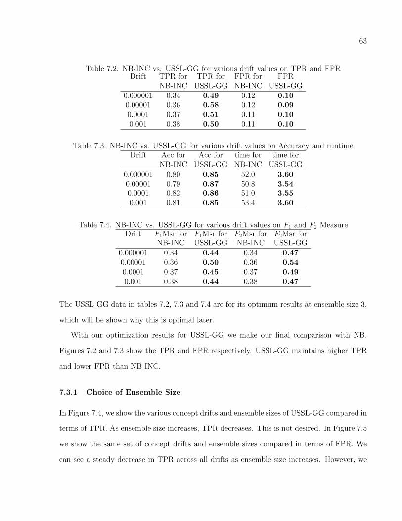
63

Table 7.2. NB-INC vs. USSL-GG for various drift values on TPR and FPRDrift TPR for TPR for FPR for FPR

NB-INC USSL-GG NB-INC USSL-GG0.000001 0.34 0.49 0.12 0.100.00001 0.36 0.58 0.12 0.090.0001 0.37 0.51 0.11 0.100.001 0.38 0.50 0.11 0.10

Table 7.3. NB-INC vs. USSL-GG for various drift values on Accuracy and runtimeDrift Acc for Acc for time for time for


Table 7.4. NB-INC vs. USSL-GG for various drift values on F1 and F2 MeasureDrift F1Msr for F1Msr for F2Msr for F2Msr for


The USSL-GG data in tables 7.2, 7.3 and 7.4 are for its optimum results at ensemble size 3,

which will be shown why this is optimal later.

With our optimization results for USSL-GG we make our final comparison with NB.

Figures 7.2 and 7.3 show the TPR and FPR respectively. USSL-GG maintains higher TPR

and lower FPR than NB-INC.

7.3.1 Choice of Ensemble Size

In Figure 7.4, we show the various concept drifts and ensemble sizes of USSL-GG compared in

terms of TPR. As ensemble size increases, TPR decreases. This is not desired. In Figure 7.5

we show the same set of concept drifts and ensemble sizes compared in terms of FPR. We

can see a steady decrease in TPR across all drifts as ensemble size increases. However, we

64

0

0.1

0.2

0.3

0.4

0.5

0.6

0.7

0.000001 0.00001 0.0001 0.001

TPR

Drift

NB-INC

USSL-GG

Figure 7.2. Comparison between NB-INC vs. our optimized model, USSL-GG in terms ofTPR

0

0.02

0.04

0.06

0.08

0.1

0.12

0.14

0.000001 0.00001 0.0001 0.001

FPR

Drift

NB-INC

USSL-GG

Figure 7.3. Comparison between NB-INC vs. our optimized model, USSL-GG in terms ofFPR

see a much larger decrease in FPR from ensemble size 1 to 2 and from 2 to 3 than from 3

to 4 and 4 to 5 across all drift values. As ensemble size increases we achieve a desired lower

FPR at the expense of also lowering TPR.

In Figure 7.6, we show that when considering the rate at which positive and negative

instances are correctly identified without punishing the algorithms for wrong classifications

with the accuracy metric, USSL-GG performs better as ensemble size increases. Figure 7.7

65

0

0.1

0.2

0.3

0.4

0.5

0.6

0.7

1 2 3 4 5

TP

R

Ensemble Size

drift .000001

drift .00001

drift .0001

drift .001

Figure 7.4. Comparison of USSL-GG across multiple drifts and ensemble sizes in terms ofTPR

0

0.05

0.1

0.15

0.2

0.25

0.3

0.35

1 2 3 4 5

FP

R

Ensemble Size

drift .000001

drift .00001

drift .0001

drift .001

Figure 7.5. Comparison of USSL-GG across multiple drifts and ensemble sizes in terms ofFPR

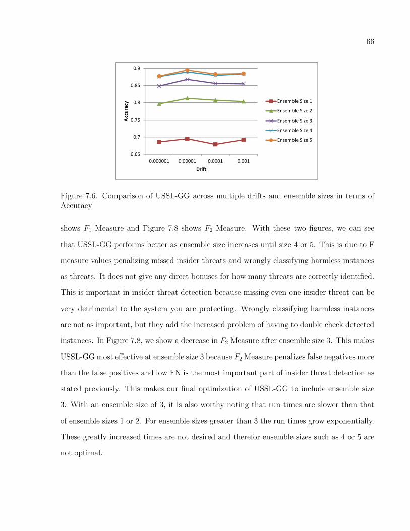
66

0.65

0.7

0.75

0.8

0.85

0.9

0.000001 0.00001 0.0001 0.001

Accuracy

Drift

Ensemble Size 1

Ensemble Size 2

Ensemble Size 3

Ensemble Size 4

Ensemble Size 5

Figure 7.6. Comparison of USSL-GG across multiple drifts and ensemble sizes in terms ofAccuracy

shows F1 Measure and Figure 7.8 shows F2 Measure. With these two figures, we can see

that USSL-GG performs better as ensemble size increases until size 4 or 5. This is due to F

measure values penalizing missed insider threats and wrongly classifying harmless instances

as threats. It does not give any direct bonuses for how many threats are correctly identified.

This is important in insider threat detection because missing even one insider threat can be

very detrimental to the system you are protecting. Wrongly classifying harmless instances

are not as important, but they add the increased problem of having to double check detected

instances. In Figure 7.8, we show a decrease in F2 Measure after ensemble size 3. This makes

USSL-GG most effective at ensemble size 3 because F2 Measure penalizes false negatives more

than the false positives and low FN is the most important part of insider threat detection as

stated previously. This makes our final optimization of USSL-GG to include ensemble size

3. With an ensemble size of 3, it is also worthy noting that run times are slower than that

of ensemble sizes 1 or 2. For ensemble sizes greater than 3 the run times grow exponentially.

These greatly increased times are not desired and therefor ensemble sizes such as 4 or 5 are

not optimal.

67

0.3

0.35

0.4

0.45

0.5

0.55

1 2 3 4 5

F1

Me

asu

re

Ensemble Size

drift .000001

drift .00001

drift .0001

drift .001

Figure 7.7. Comparison of USSL-GG across multiple drifts and ensemble sizes in terms ofF1 measure

0.42

0.44

0.46

0.48

0.5

0.52

0.54

1 2 3 4 5

F2

Me

asu

re

Ensemble Size

drift .000001

drift .00001

drift .0001

drift .001

Figure 7.8. Comparison of USSL-GG across multiple drifts and ensemble sizes in terms ofF2 measure

CHAPTER 8

SCALABILIY USING HADOOP AND MAPREDUCE

Construction of LZW dictionary and quantized dictionary is time consuming. We would

like to address scalability issues of these algorithms. One possible solution is to adopt

parallel/distributed computing. Here, we would like to exploit cloud computing based on

commodity hardware. Cloud computing is a distributed parallel solution. For our approach,

we utilize Hadoop and MapReduce based framework to facilitate parallel computing.

This chapter will be organized in the following ways. First, we will introduce Hadoop Map

Reduce(see section 8.1). Second, we will propose scalable LZW and quantized dictionary

construction algorithm using Map Reduce (MR) (see section 8.2). Finally, we will present

details results of various MR algorithms for the construction of quantized dictionary (see

section 8.3).

8.1 Hadoop Map Reduce Background

Hadoop MapReduce is a software framework that stores large volumes of data using large

clusters and retrieves relevant data in parallel from large clusters. Those large clusters are

built on a commodity hardware in a reliable fault-tolerant manner.

A map reduce job usually splits input data into a number of independent chunks. These

independent chunks will be run by map tasks in a parallel manner across clusters. Map

tasks emit intermediate key value pairs. The framework sorts output of the maps based on

intermediate keys and passes these sorted intermediate key value pairs to the reducer. The

reducer accepts the intermediate key and a list of values. Intermediate (key, value) pairs

having the same key will be directed to the same reducer. In other words, intermediate (key,

68

69

value) pairs having the same key cannot go to different reducers. However, Intermediate

(key, value) pairs having different key may end up at the same reducer.

In general, both the input and the output of the job are stored in a Hadoop distributed

file system (HDFS). Compute node is a node where map and reduce tasks are run. Storage

node is a node where HDFS is running to store chunk data. In Haddop compute node and

storage node are the same to exploit locality. In other words, map-reduce job strives to work

on the local HDFS data to save network bandwidth across clusters.

Here is a simple example for word count from a set of documents as illustrated in Fig-

ure 8.1. Splitted input files consists of a set of documents. Each line represents a document.

Each line/document is passed to individual mapper instance. Mapper emits each word as

intermediate key and value will be count 1. Intermediate output values are not usually

reduced together. All values with the same key (word) are presented to a single reducer

together. In particular, each distinct word (subset of different keyspace) is assigned to each

reducer. These subsets are known as partitioner. After shuffling and sorting, reducer will

get intermediate key (word) and a list of values (counts). In Figure 8.1 the top most reducer

will get Apple key and a list of values will be ”{1, 1, 1, 1 }”.

Algorithm 7 Word count program for MapReduce

1: Input: filename, file− contents2: Output: word, sum

3: mapper (filename, file-contents)4: for each word in file-contents do5: emit(word, 1)6: end for

7: reducer (word, values):8: sum = 09: for each value in values do

10: sum = sum+ value11: end for12: emit(word, sum)

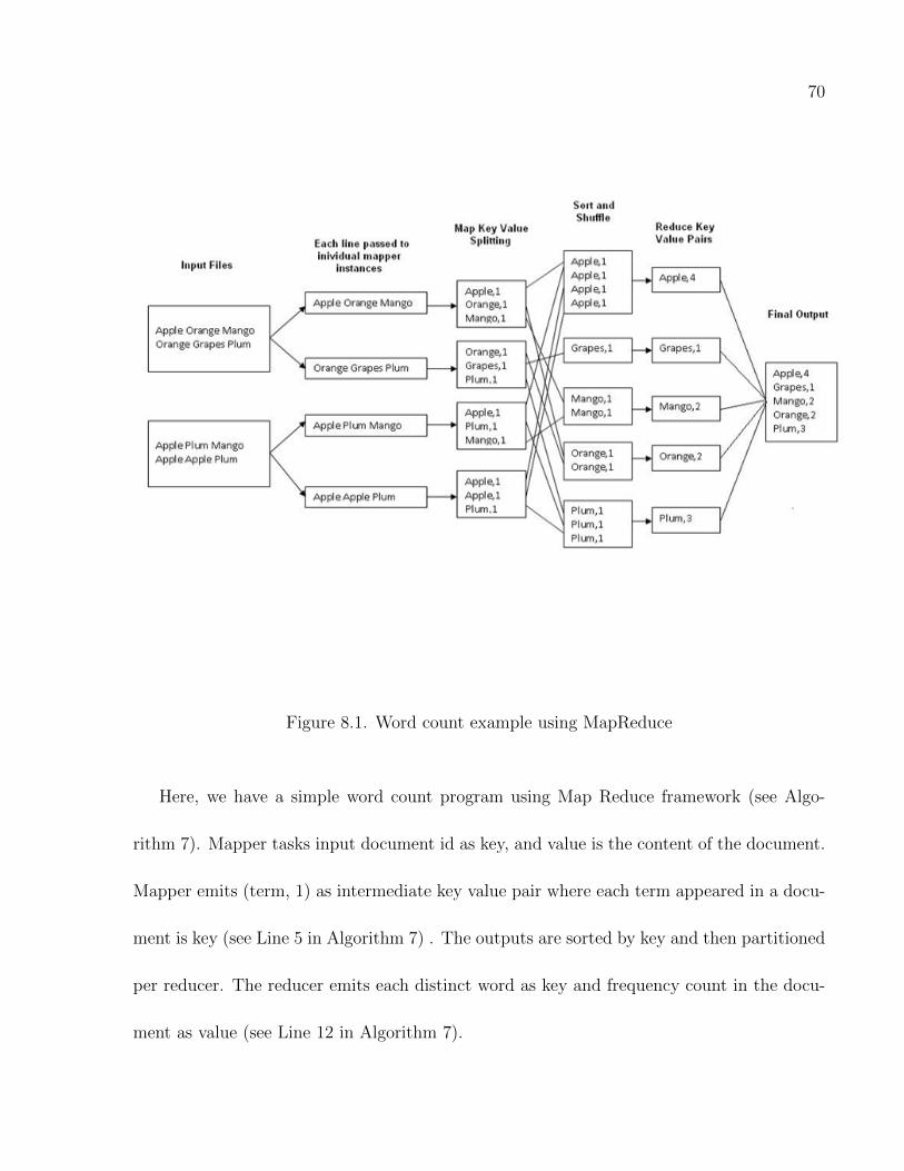
70

Figure 8.1. Word count example using MapReduce

Here, we have a simple word count program using Map Reduce framework (see Algo-

rithm 7). Mapper tasks input document id as key, and value is the content of the document.

Mapper emits (term, 1) as intermediate key value pair where each term appeared in a docu-

ment is key (see Line 5 in Algorithm 7) . The outputs are sorted by key and then partitioned

per reducer. The reducer emits each distinct word as key and frequency count in the docu-

ment as value (see Line 12 in Algorithm 7).

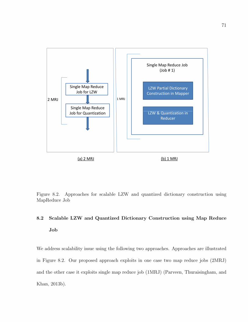
71

Single Map Reduce Job for LZW

Single Map Reduce Job for Quantization

Single Map Reduce Job(Job # 1)

LZW Partial Dictionary Construction in Mapper

LZW & Quantization in

2 MRJ 1 MRJ

Job for Quantization LZW & Quantization in Reducer

(a) 2 MRJ (b) 1 MRJ

Figure 8.2. Approaches for scalable LZW and quantized dictionary construction usingMapReduce Job

8.2 Scalable LZW and Quantized Dictionary Construction using Map Reduce

Job

We address scalability issue using the following two approaches. Approaches are illustrated

in Figure 8.2. Our proposed approach exploits in one case two map reduce jobs (2MRJ)

and the other case it exploits single map reduce job (1MRJ) (Parveen, Thuraisingham, and

Khan, 2013b).

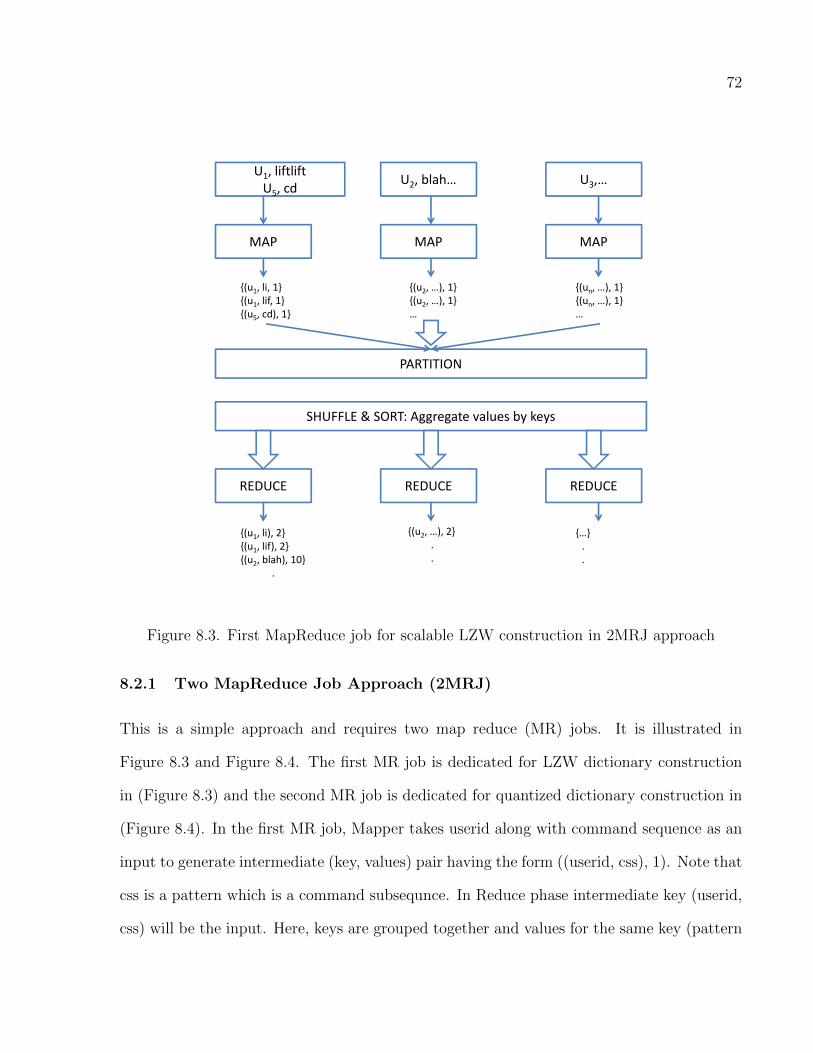
72

PARTITION

U3,…U1, liftlift

U5, cdU2, blah…

MAPMAP MAP

{(u1, li, 1}{(u1, lif, 1}{(u5, cd), 1}

{(u2, …), 1}{(u2, …), 1}…

{(un, …), 1}{(un, …), 1}…

PARTITION

SHUFFLE & SORT: Aggregate values by keys

REDUCEREDUCE REDUCE

{(u1, li), 2}{(u1, lif), 2}{(u2, blah), 10}

.

{(u2, …), 2}..

{…}..

Figure 8.3. First MapReduce job for scalable LZW construction in 2MRJ approach

8.2.1 Two MapReduce Job Approach (2MRJ)

This is a simple approach and requires two map reduce (MR) jobs. It is illustrated in

Figure 8.3 and Figure 8.4. The first MR job is dedicated for LZW dictionary construction

in (Figure 8.3) and the second MR job is dedicated for quantized dictionary construction in

(Figure 8.4). In the first MR job, Mapper takes userid along with command sequence as an

input to generate intermediate (key, values) pair having the form ((userid, css), 1). Note that

css is a pattern which is a command subsequnce. In Reduce phase intermediate key (userid,

css) will be the input. Here, keys are grouped together and values for the same key (pattern

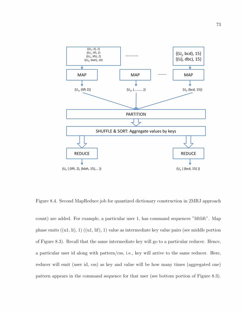
73

PARTITION

{(Uj, bcd), 15}{(Uj, dbc), 15}

{(U1, li), 2}{(U1, lif), 2}{(U1, lift), 2}

{(U2, blah), 10}

MAPMAP MAP

{U1, (lift 2)} {U2, (………..)} {Uj, (bcd, 15)}

……..

…………

PARTITION


REDUCEREDUCE

(Ui, { (lift, 2), (blah, 15),… }) (Uj, { (bcd, 15) })

Figure 8.4. Second MapReduce job for quantized dictionary construction in 2MRJ approach

count) are added. For example, a particular user 1, has command sequences ”liftlift”. Map

phase emits ((u1, li), 1) ((u1, lif), 1) value as intermediate key value pairs (see middle portion

of Figure 8.3). Recall that the same intermediate key will go to a particular reducer. Hence,

a particular user id along with pattern/css, i.e., key will arrive to the same reducer. Here,

reducer will emit (user id, css) as key and value will be how many times (aggregated one)

pattern appears in the command sequence for that user (see bottom portion of Figure 8.3).

74

Algorithm 8 presents pseudo code for LZW dictionary construction using a map reduce

job. In Algorithm 8, input file consists of line by line input. Each line has entries namely,

gname (userid) and command sequences (cseq). Next, mapper will take gname (userid) as

key and values will be command sequences for that user. In mapper we will look for patterns

having length 2, 3, etc. Here, we will check whether patterns exist in the dictionary (line 6).

If the pattern does not exist in the dictionary, we simply add that in the dictionary(line 7),

and emit intermediate key value pairs (line 8). Here, keys will be composite having gname

and pattern. Value will be frequncy count 1. At line 9 and 10, we increment pointer so that

we can look for patterns in new command sequences (cseq). If the pattern is in the dictionary,

we simply emit at line 12 and cseq’s end pointer is incremented. By not incrementing cseq’s

start pointer we will look for super-set patterns.

Combiner will be run from line 15 to line 20 in Algorithm 8. Combiner is an optional step

and acts as ”‘min reducer.” For the same user same pattern may be emitted multiple times

with frequency count 1. In combiner we aggregate them at line 18. Finally, in line 20, we emit

composite key (gname and pattern) and aggregated frequency count. Combiner helps us to

overcome unnecessary communication cost and therefore, improves processing time. Recall

that combiner is optional it may run 0 time, or 1 or many times. Hence, the signature of

combiner method (input/output parameters) need to match the output signature of mappers

and the input signature of reducers. At reducer from line 21 to 26, aggregation is carried as

shown in ”‘Combiner.”

In the second map reduce job quantization of the dictionary will be carried out (see

Figure 8.4). Mapper will carry simple transformation by generating key based on user id,

and value based on pattern frequency. In Algorithm 9, mapper will take each line as an

input from input file produced by 1st map reduce job. Here, mapper will take input (userid,

pattern) as key and frequency as value. Mapper emits intermediate key value pair where key

will be user id and value will be concatenation of pattern and frequency (see middle portion

75

of Figure 8.4 and see from line 4 to line 7 in Algorithm 9). All patterns of a particular user

and corresponding frequency will arrive at the same reducer. The reducer will conduct all

pairwise edit distance calculation among all patterns for a particular user. Finally, user id

as key and longest frequent patterns as value will be emitted by the reducer (see bottom

portion of Figure 8.4).

At the reducer, each user (gname) will be input and list of values will be patterns and

their frequency count. Here, compression of patterns will be carried out for that user. Recall

that some patterns will be pruned using Edit distance. For a user, each pattern will be stored

into Hashmap, H. Each new entry in the H will be pattern as key and value as frequency

count 1. For existing pattern in the dictionary, we will simply update frequency count(line

11). At line 13 dictionary will be quantized and H will be updated accordingly. Now, from

quantized dictionary(QD), patterns along frequency count will be emitted as values and key

will be gname (at line 14).

8.2.2 1MRJ:1 MR Job

Here, we will utilize 1 MR job. It is illustrated in Figure 8.5. We are expecting that by

reducing the number of jobs we can reduce total processing costs.

Running a job in Hadoop takes a significant overhead. Hence, by minimizing the number

of jobs, we can construct dictionary quickly. The overhead for a Hadoop job is associated with

disk I/O and network transfers. When a job is submitted to Hadoop cluster the following

actions will take place:

1. The Executable file is moved from client machine to Hadoop JobTracker1,

2. The JobTracker determines TaskTrackers2 that will execute the job,

1http://wiki.apache.org/hadoop/JobTracker

2http://wiki.apache.org/hadoop/TaskTracker

76

Algorithm 8 LZW Dictionary Construction using Map-Reduce(2MRJ)

1: Input: gname : groupname, cseq : commandsequences2: Output: Key : (gname, commandpattern(css)), count

3: map(stringgname, stringcseq)4: start← 1, end← 25: css = (csstart · · · csend)6: if css 6∈ dictionary then7: Add css to thedictionary8: emit(pairs(gname, css), integer1)9: start← start+ 1

10: end← end+ 111: else12: emit(pairs(gname, css), integer1)13: end← end+ 114: end if

15: combine(pair(gname, css), (cnt1, cnt2, · · · ))16: Sum← 017: for all cnt ∈ (cnt1, cnt2, · · · ) do18: sum← sum+ cnt19: end for20: emit(pair(gname, css), integersum)

21: reduce(pair(gname, css), (cnt1, cnt2, · · · ))22: Sum← 023: for all cnt ∈ (cnt1, cnt2, · · · ) do24: sum← sum+ cnt25: end for26: emit(pair(gname, css), integersum)

77

Algorithm 9 Compression/Quantization using Map-Reduce(2MRJ)

1: Input: line : gname, commandsequence(css), frequencycount(cnt)2: Output: Key : (gname, commandpattern(css))

3: map(stringline, string)4: gname← Spilt(line)5: css← Spilt(line)6: cnt← Spilt(line)7: emit(gname, pair(css, cnt))

8: reduce(gname, (pair(css1, cnt1), pair(css2, cnt2), · · · ))9: Sum← 0

10: for all pair(cssi, cnti) ∈ ((pair(css1, cnt1), pair(css2, cnt2) · · · ) do11: H ← H + pair(cssi, cnti)12: end for13: QD = QuantizedDictionary(H)14: emit(gname, pair(css, integer sum))15: for all cssi ∈ QD do16: emit(gname, pair(cssi, count(cssi)))17: end for

3. The Executable file is distributed to the TaskTrackers over the network,

4. Map processes initiates reading data from HDFS,

5. Map outputs are written to local discs,

6. Map outputs are read from discs, shuffled (transferred over the network to TaskTrackers

which would run Reduce processes), sorted and written to remote discs,

7. Reduce processes initiate reading the input from local discs,

8. Reduce outputs are written to discs.

Therefore, if we can reduce number of jobs we can avoid expensive disk operations and

network transfers. That is the reason we prefer 1MRJ over 2MRJ.

78

Algorithm 10 Dictionary construction and compression using single Map-Reduce(1MRJ)

1: Input: gname : groupname, cseq : commandsequences2: Output: Key : gname, commandpattern(css)

3: map(stringgname, stringcseq)4: start← 1, end← 25: css = (csstart · · · csend)6: if css 6∈ dictionary then7: Add css to thedictionary8: emit(gname, css)9: start← end

10: end← end+ 111: else12: emit(gname, css)13: end← end+ 114: end if

15: reduce(gname, (css1, css2, · · · )16: H ← 017: for all cssi ∈ ((css1, css2, · · · ) do18: if css 6∈ H then19: H ← H + (cssi, 1)20: else21: count← getfrequency(H(cssi))22: count← count+ 123: H ← H + (cssi, count)24: end if25: end for26: QD = QuantizedDictionary(H)27: for all cssi ∈ QD do28: emit(gname, pair(cssi, count(cssi)))29: end for

79

Mapper will emit user id as key and value will be pattern (see Algorithm 10). Recall

that in mapper partial LZW operation will be completed. The same user id will arrive at

the same reducer since user is the intermediate key. For that user id, a reducer will have a

list of patterns. In the reducer, incomplete LZW will be completed here. In addition, full

quantization operation will be implemented as described in Chapter 6.2.1. Parallelization

will be achieved at the user level (inter-user parallelization) instead of within users (intra-

user parallelization). In mapper, parallelization will be carried out by dividing large files

into a number of chunks and process a certain number of files in parallel.

Algorithm 10 illustrates the idea. Input file consists of line by line input. Each line

has entries namely, gname (userid) and command sequences (cseq). Next, mapper will take

gname (userid) as key, and values will be command sequences for that user. In mapper we

will look for patterns having length 2, 3, etc. Here, we will check whether patterns exist

in the dictionary (line 6). If the pattern does not exist in the dictionary, we simply add

that in the dictionary(line 7), and emit intermediate key value pairs (line 8) having keys as

gname and values as patterns with length 2, 3 etc. At line 9 and 10, we increment pointer

so that we can look for patterns in new command sequences (cseq). If the pattern is in the

dictionary, we simply emit at line 12 and cseq’s end pointer is incremented so that we can

look for super-set command sequence.

At the reducer, each user (gname) will be input and list of values will be patterns. Here,

compression of patterns will be carried for that user. Recall that some patterns will be

pruned using Edit distance. For a user each pattern will be stored into Hashmap, H. Each

new entry in the H will be pattern as key and value as frequency count. For existing pattern

in the dictionary, we will simply update frequency count(line 18). At line 20 dictionary will

be quantized, and H will be updated accordingly. Now, from quantized dictionary all distinct

patterns from H will emitted as values along with key gname.

80

8.3 Experimental Setup and Results

8.3.1 Hadoop Cluster

Our hadoop cluster (cshadoop0-cshadoop9) is compromised of virtual machines that run in

the Computer Science vmware esx cloud - so there are 10 VM’s. Each VM is configured as

a quad core with 4GB of ram and a 256GB virtual hard drive. The virtual hard drives are

stored on the CS SAN (3PAR).

There are three ESX hosts which are Dell Poweredge R720’s with 12 cores @2.99GHZ,

128GB of RAM, and fiber to the 3PAR SAN. The VM’s are spread across the three ESX

hosts in order to balance the load.

”cshadoop0” is configured as the ”name node”. A”cshadoop1” through ”cshadoop9” are

configured as the slave ”data nodes”.

We have implemented our approach using Java JDK version 1.6.0.39. For MapReduce

implementation we have used Hadoop version 1.0.4.

8.3.2 Big Dataset for Insider Threat Detection

The Data sets used are created from the trace files from the University of Calgary project.

168 files have been collected from different levels of users of UNIX as described in (Greenberg,

1988; Maxion, 2003). The different levels of users are:

• Novice programmers (56 users)

• Experienced programmers (36 users)

• Computer scientists (52 Users)

• Non-programmers (25 users).

Each file contains the commands used by each of the users over weeks.

81

Now, in order to get the big data, first we replicated the user files randomly so that we

have:

• Novice programmers - (1320 Users) i.e. File starting from ”novice-0001” till ”novice-

1320”

• Experienced programmers - (576 Users)

• Computer scientists - (832 Users)

• Non-programmers - (1600 Users)

Total Number of Users = 4328; size is 430 MB; and one command file is for one user.

Next, we gave these files as input to our program (written in Python) which gave unique

unicode for each distinct command provided by all users. The output file for all users is 15.5

MB. We dubbed it as original data (OD).

Finally, we replicated this data 12 times for each user. And we ended up 187 MB of input

file which was given as an input to Map Reduce job of LZW and Compression. We dubbed

as duplicate big data (DBD).

8.3.3 Results for Big Data Set Related to Insider Threat Detection

First, we experiment on OD, and next, we concentrate on DBD.

On OD Dataset:

We have compared our approaches namely, 2MRJ and 1MRJ on OD dataset. Here, we

have varied number of reducers and fixed number of mappers (e.g., HDFS block size equals

64MB). In case 2MRJ, we have varied a number of reducers in 2nd job’s reducer and not

in first map reduce job. 1MRJ outperforms 2MRJ in terms of processing time on a fixed

number of reducers except in the first case (number reducer equals to 1). With the latter

82

PARTITION

Un,…Um,…

U1, liftliftU5, blahblah

U2, blah…

MAPMAP MAP

(U1, li)(U1, lif)(U1, lift),…

(U2, Bl)(U2, Bla)(U2, Blah),…

(Un, …)(Un, …)(Um, …)

PARTITION


REDUCE

(U1, {(lift,2), (blah, 15) })(U2, {(blah, 15)})

REDUCE REDUCE

Quantization

Figure 8.5. 1MRJ: 1 MR Job approach for scalable LZW and quantized dictionary construc-tion

case, parallelization is limited at the reducer phase. Table 8.1 illustrates this. For example,

for number of reducer equals 9, total time taken is 3.47 sec and 2.54 sec for 2MRJ and 1MRJ

approaches respectively.

With regard to 2MRJ case, Table 8.3 presents input-output statistics of both MapReduce

jobs. For example, for first map reduce job mapper emits 65,37,040 intermediate key value

pairs and Reducer emits 95.75MB output. This 95.75MB will be the input for mapper for

the second MapReduce job.

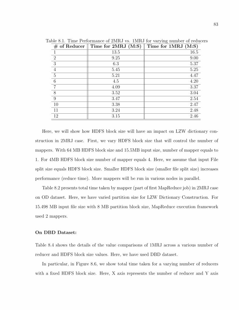
83

Table 8.1. Time Performance of 2MRJ vs. 1MRJ for varying number of reducers# of Reducer Time for 2MRJ (M:S) Time for 1MRJ (M:S)1 13.5 16.52 9.25 9.003 6.3 5.374 5.45 5.255 5.21 4.476 4.5 4.207 4.09 3.378 3.52 3.049 3.47 2.5410 3.38 2.4711 3.24 2.4812 3.15 2.46

Here, we will show how HDFS block size will have an impact on LZW dictionary con-

struction in 2MRJ case. First, we vary HDFS block size that will control the number of

mappers. With 64 MB HDFS block size and 15.5MB input size, number of mapper equals to

1. For 4MB HDFS block size number of mapper equals 4. Here, we assume that input File

split size equals HDFS block size. Smaller HDFS block size (smaller file split size) increases

performance (reduce time). More mappers will be run in various nodes in parallel.

Table 8.2 presents total time taken by mapper (part of first MapReduce job) in 2MRJ case

on OD dataset. Here, we have varied partition size for LZW Dictionary Construction. For

15.498 MB input file size with 8 MB partition block size, MapReduce execution framework

used 2 mappers.

On DBD Dataset:

Table 8.4 shows the details of the value comparisons of 1MRJ across a various number of

reducer and HDFS block size values. Here, we have used DBD dataset.

In particular, in Figure 8.6, we show total time taken for a varying number of reducers

with a fixed HDFS block size. Here, X axis represents the number of reducer and Y axis

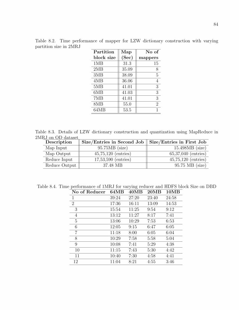
84

Table 8.2. Time performance of mapper for LZW dictionary construction with varyingpartition size in 2MRJ

Partition Map No ofblock size (Sec) mappers1MB 31.3 152MB 35.09 83MB 38.09 54MB 36.06 45MB 41.01 36MB 41.03 37MB 41.01 38MB 55.0 264MB 53.5 1

Table 8.3. Details of LZW dictionary construction and quantization using MapReduce in2MRJ on OD dataset

Description Size/Entries in Second Job Size/Entries in First JobMap Input 95.75MB (size) 15.498MB (size)Map Output 45,75,120 (entries) 65,37,040 (entries)Reduce Input 17,53,590 (entries) 45,75,120 (entries)Reduce Output 37.48 MB 95.75 MB (size)

Table 8.4. Time performance of 1MRJ for varying reducer and HDFS block Size on DBDNo of Reducer 64MB 40MB 20MB 10MB1 39:24 27:20 23:40 24:582 17:36 16:11 13:09 14:53

3 15:54 11:25 9:54 9:124 13:12 11:27 8:17 7:415 13:06 10:29 7:53 6:536 12:05 9:15 6:47 6:057 11:18 8:00 6:05 6:048 10:29 7:58 5:58 5:049 10:08 7:41 5:29 4:3810 11:15 7:43 5:30 4:4211 10:40 7:30 4:58 4:41

12 11:04 8:21 4:55 3:46

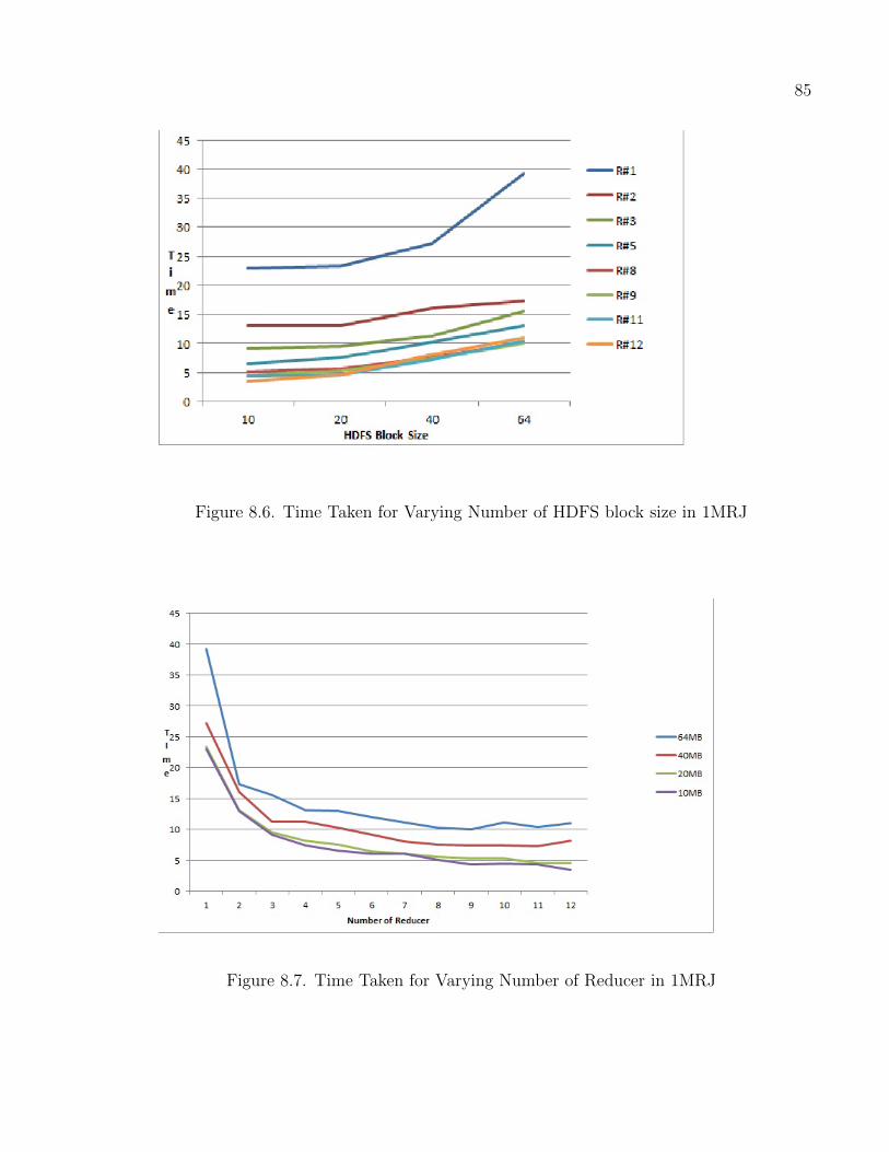
85

Figure 8.6. Time Taken for Varying Number of HDFS block size in 1MRJ

Figure 8.7. Time Taken for Varying Number of Reducer in 1MRJ

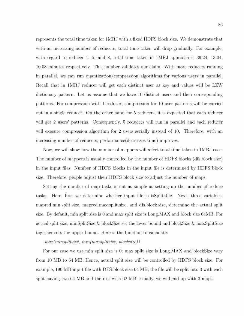
86

represents the total time taken for 1MRJ with a fixed HDFS block size. We demonstrate that

with an increasing number of reducers, total time taken will drop gradually. For example,

with regard to reducer 1, 5, and 8, total time taken in 1MRJ approach is 39.24, 13.04,

10.08 minutes respectively. This number validates our claim. With more reducers running

in parallel, we can run quantization/compression algorithms for various users in parallel.

Recall that in 1MRJ reducer will get each distinct user as key and values will be LZW

dictionary pattern. Let us assume that we have 10 distinct users and their corresponding

patterns. For compression with 1 reducer, compression for 10 user patterns will be carried

out in a single reducer. On the other hand for 5 reducers, it is expected that each reducer

will get 2 users’ patterns. Consequently, 5 reducers will run in parallel and each reducer

will execute compression algorithm for 2 users serially instead of 10. Therefore, with an

increasing number of reducers, performance(decreases time) improves.

Now, we will show how the number of mappers will affect total time taken in 1MRJ case.

The number of mappers is usually controlled by the number of HDFS blocks (dfs.block.size)

in the input files. Number of HDFS blocks in the input file is determined by HDFS block

size. Therefore, people adjust their HDFS block size to adjust the number of maps.

Setting the number of map tasks is not as simple as setting up the number of reduce

tasks. Here, first we determine whether input file is isSplitable. Next, three variables,

mapred.min.split.size, mapred.max.split.size, and dfs.block.size, determine the actual split

size. By default, min split size is 0 and max split size is Long.MAX and block size 64MB. For

actual split size, minSplitSize & blockSize set the lower bound and blockSize & maxSplitSize

together sets the upper bound. Here is the function to calculate:

max(minsplitsize, min(maxsplitsize, blocksize))

For our case we use min split size is 0; max split size is Long.MAX and blockSize vary

from 10 MB to 64 MB. Hence, actual split size will be controlled by HDFS block size. For

example, 190 MB input file with DFS block size 64 MB, the file will be split into 3 with each

split having two 64 MB and the rest with 62 MB. Finally, we will end up with 3 maps.

87

In Figure 8.7 we show the impact of HDFS block size on total time taken for a fixed

number of reducers. Here, X axis represents HDFS block size and Y axis represents total

time taken for 1MR approach with a fixed number of reducers. We demonstrate that with

increasing number of HDFS block size, total time taken will increase gradually for a fixed

input file. For example, with regard to HDFS block size 10, 20, 40, 64 MB total time taken

in 1MRJ approach were 7.41, 8.17, 11.27, 13.12 minute respectively for a fixed number of

reducers (=4). On one hand, when HDFS block size of 10 MB, and input file is 190 MB,

19 maps run where each map processes 10MB input split. On the other hand, for HDFS

block size=64 MB, 3 maps will be run where each map will process a 64 MB input split. In

the former case (19 maps with 10 MB) each map will process a smaller file and in the latter

case (3 maps with 64 MB) we process a larger file which consequently consumes more time.

In the former case, more parallelization can be achieved. In our architecture, more than 10

mappers can be run in parallel. Hence, for a fixed input file and fixed number of reducers,

total time increases with increasing HDFS block size.

CHAPTER 9

CONCLUSIONS AND FUTURE WORK

9.1 Conclusion

Insider threat detection is a very important problem requiring critical attention. This dis-

sertation presents a number of approaches to detect insider threats through augmented un-

supervised and supervised learning techniques on evolving stream. Here, we have considered

sequence and non sequence stream data.

The supervised learning approach to insider threat detection outperformed the unsuper-

vised learning approach. The supervised method succeeded in identifying all 12 anomalies

in the 1998 Lincoln Laboratory Intrusion Detection dataset with zero false negatives and a

lower false positive rate than the unsupervised approach.

For unsupervised learning, Graph-based anomaly detection (GBAD) (Cook and Holder,

2007; Eberle and Holder, 2007; Cook and Holder, 2000) is used. However, applying GBAD

to the insider threat problem requires an approach that is sufficiently adaptive and efficient

so effective models can be built from vast amounts of evolving data.

The technique combines the power of GBAD and one-class SVMS with the adaptiveness

of stream mining to achieve effective practical insider threat detection for unbounded evolv-

ing data streams. Increasing the weighted cost of false negatives increased accuracy and

ultimately allowed our approach to perform well. Though false positives could be further

reduced through more parameter tuning, our approach accomplished the goal of detecting

all insider threats.

We examine the problem of insider threat detection in the context of command sequences

and propose an unsupervised ensemble based learning approach that can take into account

88

89

concept drift. The approach adopts advantages of both compression and incremental learn-

ing. A classifier is typically built and trained using large amount of legitimate data. However,

training a classifier is very expensive, and furthermore, it has problems when the baseline

changes, as is the case in real life networks. We acknowledge this continuously changing fea-

ture of legitimate actions, and introduce the notion of concept drift to address the changes.

The proposed unsupervised learning system adapts directly to the changes in command se-

quence data. In addition, to improve accuracy, we use an ensemble of K classifiers, instead

of a single one. Voting is used, and a subset of classifiers is used because classifiers with more

recent data gradually replace those that are outdated. We address an important problem

and propose a novel approach.

For sequence data, our stream guided sequence learning performed well, with limited num-

ber of false positives as compared to static approaches. This is because the approach adopts

advantages from both compression & ensemble-based learning. In particular, compression

offered unsupervised learning in a manageable manner and on the other hand ensemble based

learning offered adaptive learning. The approach was tested on real command line dataset

and shows effectiveness over static approaches in terms of TP and FP.

Compressed/quantized dictionary construction is computationally expensive. It does not

scale well with a number of users. Hence, we look for distributed solution with parallel com-

puting with commodity hardware. For this, all users’ quantized dictionary is constructed

using a MapReduce framework on Hadoop. A number of approaches are suggested, ex-

perimented on benchmark dataset, and discussed. We have shown with 1 map reduce job

that quantized dictionary can be constructed and demonstrates effectiveness over other ap-

proaches.

9.2 Future Work

We would like to extend the work in the following directions.

90

9.2.1 Incorporate User Feedback

For unsupervised learning, we assume that no ground truth is available. In fact, over time

some ground truth may be available in terms of feedback. Once a model is created in an

unsupervised manner, we would like to update the model based on user feedback. Right

now, once the model is created it remains unchanged. When ground truth is available over

time, we will refine our all models based on this feedback immediately (Masud et al., 2010).

9.2.2 Collusion Attack

During unsupervised learning (see Chapter 4), when we update models, collusion at-

tack (Zhao et al., 2005; Wang et al., 2009) may take place. In that case, a set of models

among K models will not be replaced for a while. Each time, when a victim will be selected,

these colluded models will survive. Recall that ”collusion” is an agreement between two or

more models so that they will always agree on the prediction. In particular, if we have K = 3

models, two models may maintain secretive agreement and their prediction will be the same

and used as ground truth. Therefore, two colluded/secretive models will always survive and

never be victim in model update case. Recall that the learning is unsupervised and majority

voting will be taken as ground truth. Hence, we will not be able to catch insider attack. Our

goal is to identify colluded attack. For this, during victim selection of models, we will take

into account agreement of models over time. If agreement of models persists for a long time

and survive, we will choose the victim from there.

9.2.3 Additional Experiment

We will do additional experiment on more sophisticated scenarios, including chunk size.

Currently, we assume that chunk size is fixed or uniform. Fixed chunk is easy to implement.

But it fails to capture concept drift or anomaly in the stream. Assume that concept drift

happens at the end of a chunk (fixed size). We may not be able to detect anomaly until

91

we process the next chunk. For this, the better approach will be creation of dynamic chunk

size. Here, chunk size will vary. Variable chunk size will be estimated by using change point

detection (Cangussu and Baron, 2006; Baron and Tartakovsky, 2006). Once we observe a

new distribution, current chunk ends, and new chunk will emerge.

Instead of one class SVM, we may use other classifiers (Parveen and Thuraisingham,

2006). When we apply insider threat detection across multiple data sources/domains we

need to address heterogeneity issues of schema/sources. For this, we will utilize schema

matching/ontology alignment (Partyka et al., 2011; Alipanah, Parveen et al., 2010; Alipanah

et al., 2011; Alipanah, Srivastava et al., 2010; Khan and Luo, 2002; Khan et al., 2004).

9.2.4 Anomaly Detection in Social Network and Author Attribution

Anomaly detection will be carried out in social network using our proposed supervised and

unsupervised approaches.

Twitter, on line social network, allows friends to communicate and stays connected via

exchanging short messages (140 character). Spammer presence is prevalent in twitter now.

Spammers post malicious links, send unsolicited messages to legitimate users and hijack

trending topics in twitter. At least 3% of messages can be categorized as spammers. We can

extend our framework to detect spammer by exploiting anomaly detection.

New authors may appear in blog. Our goal is to identify these new authors in the

stream. For this, our anomaly detection can be applied. Feature extraction needs to be

changed (i.e., stylometric feature (Jamak et al., 2012)). We would like to carry out our

techniques for author attribution (Akiva and Koppel, 2012; Koppel et al., 2009; Seker et al.,

2013).

9.2.5 Stream mining as a Big data mining problem

Stream data can be treated as big data.

92

This is due to well-known properties of stream data such as infinite length, high speed

data arrival, online/timely data processing, changing characteristics of data and need for

one-pass techniques (i.e., forgotten raw data) etc. In particular, data streams are infinite,

therefore efficient storage and incremental learning are required. The underlying concept

changes over time are known as concept drift. The learner should adapt to this change and

be ready for veracity and variety. New classes evolving in the stream are known as concept

evolution, which make classification difficult. New features may also evolve in the stream,

such as text streams.

All of these properties conform to characteristics of big data. For example, infinite length

of stream data constitutes large ”Volume” of big data. High speed data arrival and on-line

processing holds the characteristics of large ”Velocity” of big data. Stream data can be

sequence or non sequnce data (vector). This conforms ”verity” characteristics of big data.

Characteristics of stream data can be changed over time. New patterns may emerge in

evolving stream. Old patterns may be outdated. These properties may support the notion

of ”Veracity” of big data. Therefore, stream data possesses characteristics of big data. In

spite of the success and extensive studies of stream mining techniques, there is no single

work dedicated to a unified study of the new challenges introduced by big data and evolving

stream data.

The big data community adopts big data infrastructures that are used to process un-

bounded continuous streams of data (e.g., S4, Storm). However, their data mining support

is rudimentary. A number of open source tools for big data mining have been released to

support traditional data mining. Only a few tools support very basic stream mining. Re-

search challenges such as change detection, novelty detection, and feature evolution over

evolving streams have been recently studied in traditional stream mining (Domingos and

Hulten, 2001; Davison and Hirsh, 1998; Masud, Chen, Gao, Khan, Aggarwal et al., 2010;

Masud et al., 2011a; Fan, 2004) but not in big data.

93

Here, we need a unified picture of how these challenges and proposed solutions can be

augmented in these open source tools. In addition to presenting the solutions to overcome

stream mining challenges, experience with real applications of these techniques to data min-

ing and security will be shared across the world.

• Big Data Stream Infrastructure: Apache S4 (Neumeyer et al., 2010), Storm, Cassan-

dra (Lakshman and Malik, 2010) etc including batch processing Hadoop.

• Big Data Mining Tool: Apache Mahout (Owen et al., 2011), MOA (Zliobaite et al.,

2011), PEGASUS (Kang et al., 2011), GraphLab, SAMOA and their support for

Stream Mining.

REFERENCES

Abouzeid, A., K. Bajda-Pawlikowski, D. J. Abadi, A. Rasin, and A. Silberschatz (2009).Hadoopdb: An architectural hybrid of mapreduce and dbms technologies for analyticalworkloads. PVLDB 2 (1), 922–933.

Akiva, N. and M. Koppel (2012). Identifying distinct components of a multi-author docu-ment. In EISIC, pp. 205–209.

Al-Khateeb, T., M. M. Masud, L. Khan, C. C. Aggarwal, J. Han, and B. M. Thuraisingham(2012). Stream classification with recurring and novel class detection using class-basedensemble. In ICDM, pp. 31–40.

Al-Khateeb, T., M. M. Masud, L. Khan, and B. M. Thuraisingham (2012). Cloud guidedstream classification using class-based ensemble. In IEEE CLOUD, pp. 694–701.

Alipanah, N., P. Parveen, L. Khan, and B. M. Thuraisingham (2011). Ontology-drivenquery expansion using map/reduce framework to facilitate federated queries. In ICWS,pp. 712–713.

Alipanah, N., P. Parveen, S. Menezes, L. Khan, S. Seida, and B. M. Thuraisingham (2010).Ontology-driven query expansion methods to facilitate federated queries. In SOCA, pp.1–8.

Alipanah, N., P. Srivastava, P. Parveen, and B. M. Thuraisingham (2010). Ranking ontologiesusing verified entities to facilitate federated queries. In Web Intelligence, pp. 332–337.

Baron, M. and A. Tartakovsky (2006). Asymptotic optimality of change-point detectionschemes in general continuous-time models. Sequential Analysis 25 (3), 257–296.

Borges, E. N., M. G. de Carvalho, R. Galante, M. A. Goncalves, and A. H. F. Laender (2011,sep). An unsupervised heuristic-based approach for bibliographic metadata deduplication.Inf. Process. Manage. 47 (5), 706–718.

Brackney, R. C. and R. H. Anderson (Eds.) (2004, March). Understanding the Insider Threat.RAND Corporation.

Bu, Y., B. Howe, M. Balazinska, and M. Ernst (2010). Haloop: Efficient iterative dataprocessing on large clusters. PVLDB 3 (1), 285–296.

94

95

Burrows, M. (2006). The chubby lock service for loosely-coupled distributed systems. InOSDI, pp. 335–350.

Cangussu, J. W. and M. Baron (2006). Automatic identification of change points for thesystem testing process. In COMPSAC (1), pp. 377–384.

Chang, C.-C. and C.-J. Lin (2011). LIBSVM: a library for support vector machines. In ACMTransactions on Intelligent Systems and Technology, pp. 2:27:1–27:27. Software availableat http://www.csie.ntu.edu.tw/ cjlin/libsvm.

Chang, F., J. Dean, S. Ghemawat, W. C. Hsieh, D. A. Wallach, M. Burrows, T. Chandra,A. Fikes, and R. Gruber (2006). Bigtable: A distributed storage system for structureddata (awarded best paper!). In OSDI, pp. 205–218.

Chang, F., J. Dean, S. Ghemawat, W. C. Hsieh, D. A. Wallach, M. Burrows, T. Chandra,A. Fikes, and R. E. Gruber (2008). Bigtable: A distributed storage system for structureddata. ACM Trans. Comput. Syst. 26 (2).

Chen, L., S. Zhang, and L. Tu (2009). An algorithm for mining frequent items on data streamusing fading factor. In Proc. IEEE International Computer Software and ApplicationsConference (COMPSAC), pp. 172–177.

Chu, C. T., S. K. Kim, Y. A. Lin, Y. Yu, G. R. Bradski, A. Y. Ng, and K. Olukotun(2006). Map-reduce for machine learning on multicore. In B. Scholkopf, J. C. Platt, andT. Hoffman (Eds.), NIPS, pp. 281–288. MIT Press.

Chua, S.-L., S. Marsland, and H. W. Guesgen (2011). Unsupervised learning of patterns indata streams using compression and edit distance. In IJCAI, pp. 1231–1236.

Cook, D. J. and L. B. Holder (2000). Graph-based data mining. IEEE Intelligent Sys-tems 15 (2), 32–41.

Cook, D. J. and L. B. Holder (Eds.) (2007). Mining Graph Data. Hoboken, New Jersey:John Wiley & Sons, Inc.

Davison, B. D. and H. Hirsh (1998). Predicting sequences of user actions. in working notesof the joint workshop on predicting the future: Ai approches to time series analysis. In15th National Conference on Artificial Intelligence and Machine, pp. 5–12. AAAI Press.

Dean, J. and S. Ghemawat (2008, January). Mapreduce: simplified data processing on largeclusters. Commun. ACM 51, 107–113.

DeCandia, G., D. Hastorun, M. Jampani, G. Kakulapati, A. Lakshman, A. Pilchin, S. Siva-subramanian, P. Vosshall, and W. Vogels (2007). Dynamo: amazon’s highly availablekey-value store. In T. C. Bressoud and M. F. Kaashoek (Eds.), SOSP, pp. 205–220. ACM.

96

Ding, L., T. Finin, Y. Peng, P. P. da Silva, and D. L. Mcguinness (2005). Tracking rdf graphprovenance using rdf molecules.

Domingos, P. and G. Hulten (2001). Catching up with the Data: Research Issues in MiningData Streams. In DMKD.

Domingos, P. and G. Hulten (2000). Mining high-speed data streams. In Proc. ACMSIGKDD, Boston, MA, USA, pp. 71–80. ACM Press.

Eagle, N. and A. (Sandy) Pentland (2006, March). Reality mining: sensing complex socialsystems. Personal Ubiquitous Comput. 10 (4), 255–268.

Eberle, W., J. Graves, and L. Holder (2011). Insider threat detection using a graph-basedapproach. Journal of Applied Security Research 6 (1), 32–81.

Eberle, W. and L. B. Holder (2007). Mining for structural anomalies in graph-based data.In Proc. International Conference on Data Mining (DMIN), pp. 376–389.

Eskin, E., A. Arnold, M. Prerau, L. Portnoy, and S. Stolfo (2002). A geometric framework forunsupervised anomaly detection: Detecting intrusions in unlabeled data. In D. Barbaraand S. Jajodia (Eds.), Applications of Data Mining in Computer Security, Chapter 4.Springer.

Eskin, E., M. Miller, Z.-D. Zhong, G. Yi, W.-A. Lee, and S. Stolfo (2000). Adaptive modelgeneration for intrusion detection systems. In Proc. ACM CCS Workshop on IntrusionDetection and Prevention (WIDP).

Fan, W. (2004). Systematic data selection to mine concept-drifting data streams. In Proc.ACM SIGKDD, Seattle, WA, USA, pp. 128–137.

Forrest, S., S. A. Hofmeyr, A. Somayaji, and T. A. Longstaff (1996). A sense of self forUnix processes. In Proc. IEEE Symposium on Computer Security and Privacy (S&P), pp.120–128.

Gao, D., M. K. Reiter, and D. Song (2004). On gray-box program tracking for anomalydetection. In Proc. USENIX Security Symposium, pp. 103–118.

Greenberg, S. (1988). Using unix: Collected traces of 168 users. In Research Report88/333/45, Department of Computer Science, University of Calgary, Calgary, Canada.http://grouplab.cpsc.ucalgary.ca/papers/.

Hampton, M. P. and M. Levi (1999). Fast spinning into oblivion? recent developmentsin money-laundering policies and offshore finance centres. Third World Quarterly 20 (3),645–656.

97

Haque, A., B. Parker, and L. Khan (2013a). Intelligent mapreduce based frameworks forlabeling instances in evolving data stream. In CloudCom.

Haque, A., B. Parker, and L. Khan (2013b). Labeling instances in evolving data streamswith mapreduce. In BigData.

Hofmeyr, S. A., S. Forrest, and A. Somayaji (1998). Intrusion detection using sequences ofsystem calls. Journal of Computer Security 6 (3), 151–180.

Husain, M., P. Doshi, L. Khan, and B. Thuraisingham (2009). Storage and retrieval of largerdf graph using hadoop and mapreduce. In Proceedings of the 1st International Conferenceon Cloud Computing, CloudCom ’09, Berlin, Heidelberg, pp. 680–686. Springer-Verlag.

Husain, M. F., L. Khan, M. Kantarcioglu, and B. Thuraisingham (2010). Data intensivequery processing for large rdf graphs using cloud computing tools. In Proceedings of the2010 IEEE 3rd International Conference on Cloud Computing, CLOUD ’10, Washington,DC, USA, pp. 1–10. IEEE Computer Society.

Husain, M. F., J. P. McGlothlin, M. M. Masud, L. R. Khan, and B. M. Thuraisingham(2011). Heuristics-based query processing for large rdf graphs using cloud computing.IEEE Trans. Knowl. Data Eng. 23 (9), 1312–1327.

Jamak, A., S. A., and M. Can (2012). Principal component analysis for authorship attribu-tion. Business Systems Research 3 (2), 49–56.

Ju, W.-H. and Y. Vardi (2001, June). A hybrid high-order markov chain model for computerintrusion detection. Journal of Computational and Graphical Statistics .

Kang, U., C. E. Tsourakakis, and C. Faloutsos (2011). Pegasus: mining peta-scale graphs.Knowl. Inf. Syst. 27 (2), 303–325.

Kendall, K. (1998). A database of computer attacks for the evaluation of intrusion detectionsystems. Master’s thesis, Massachusetts Institute of Technology.

Ketkar, N. S., L. B. Holder, and D. J. Cook (2005). Subdue: Compression-based frequentpattern discovery in graph data. In Proc. ACM KDD Workshop on Open-Source DataMining.

Khan, L. and F. Luo (2002). Ontology construction for information selection. In ICTAI, pp.122–.

Khan, L., D. McLeod, and E. H. Hovy (2004). Retrieval effectiveness of an ontology-basedmodel for information selection. VLDB J. 13 (1), 71–85.

Koppel, M., J. Schler, and S. Argamon (2009). Computational methods in authorship attri-bution. JASIST 60 (1), 9–26.

98

Kowalski, E., T. Conway, S. Keverline, M. Williams, D. Cappelli, B. Willke, and A. Moore(2008, January). Insider threat study: Illicit cyber activity in the government sector.Technical report, U.S. Department of Homeland Security, U.S. Secret Service, CERT, andthe Software Engineering Institute (Carnegie Mellon University).

Kranen, P., H. Kremer, T. Jansen, T. Seidl, A. Bifet, G. Holmes, B. Pfahringer, and J. Read(2012). Stream data mining using the moa framework. In DASFAA (2), pp. 309–313.

Krugel, C., D. Mutz, F. Valeur, and G. Vigna (2003). On the detection of anomalous systemcall arguments. In Proc. 8th European Symposium on Research in Computer Security(ESORICS), pp. 326–343.

Lakshman, A. and P. Malik (2010, April). Cassandra: a decentralized structured storagesystem. SIGOPS Oper. Syst. Rev. 44 (2), 35–40.

Liao, Y. and V. R. Vemuri (2002). Using text categorization techniques for intrusion detec-tion. In Proc. 11th USENIX Security Symposium, pp. 51–59.

Liu, A., C. Martin, T. Hetherington, and S. Matzner (2005). A comparison of system callfeature representations for insider threat detection. In Proc. IEEE Information AssuranceWorkshop (IAW), pp. 340–347.

Manevitz, L. M. and M. Yousef (2002, March). One-class svms for document classification.In The Journal of Machine Learning Research, pp. 2.

Masud, M. M., T. Al-Khateeb, L. Khan, C. C. Aggarwal, J. Gao, J. Han, and B. M. Thu-raisingham (2011). Detecting recurring and novel classes in concept-drifting data streams.In ICDM, pp. 1176–1181.

Masud, M. M., Q. Chen, J. Gao, L. Khan, C. Aggarwal, J. Han, and B. Thuraisingham(2010). Addressing concept-evolution in concept-drifting data streams. In Proc. IEEEInternational Conference on Data Mining (ICDM), pp. 929–934.

Masud, M. M., Q. Chen, J. Gao, L. Khan, J. Han, and B. M. Thuraisingham (2010).Classification and novel class detection of data streams in a dynamic feature space. InECML/PKDD (2), pp. 337–352.

Masud, M. M., Q. Chen, L. Khan, C. C. Aggarwal, J. Gao, J. Han, A. N. Srivastava, andN. C. Oza (2013). Classification and adaptive novel class detection of feature-evolvingdata streams. IEEE Trans. Knowl. Data Eng. 25 (7), 1484–1497.

Masud, M. M., J. Gao, L. Khan, J. Han, and B. Thuraisingham (2008). A practical approachto classify evolving data streams: Training with limited amount of labeled data. In Proc.IEEE International Conference on Data Mining (ICDM), pp. 929–934.

99

Masud, M. M., J. Gao, L. Khan, J. Han, and B. M. Thuraisingham (2010). Classification

and novel class detection in data streams with active mining. In PAKDD (2), pp. 311–324.

Masud, M. M., J. Gao, L. Khan, J. Han, and B. M. Thuraisingham (2011a). Classification

and novel class detection in concept-drifting data streams under time constraints. IEEE

Trans. Knowl. Data Eng. (TKDE) 23 (6), 859–874.

Masud, M. M., J. Gao, L. Khan, J. Han, and B. M. Thuraisingham (2011b). Classification

and novel class detection in concept-drifting data streams under time constraints. IEEE

Trans. Knowl. Data Eng. 23 (6), 859–874.

Masud, M. M., C. Woolam, J. Gao, L. Khan, J. Han, K. W. Hamlen, and N. C. Oza

(2011). Facing the reality of data stream classification: coping with scarcity of labeled

data. Knowl. Inf. Syst. 33 (1), 213–244.

Matzner, S. and T. Hetherington (2004). Detecting early indications of a malicious insider.

IA Newsletter 7 (2), 42–45.

Maxion, R. A. (2003). Masquerade detection using enriched command lines. In Proc. IEEE

International Conference on Dependable Systems & Networks (DSN), pp. 5–14.

Moretti, C., K. Steinhaeuser, D. Thain, and N. V. Chawla (2008). Scaling up classifiers to

cloud computers. In Proceedings of the 2008 Eighth IEEE International Conference on

Data Mining, Washington, DC, USA, pp. 472–481. IEEE Computer Society.

Neumeyer, L., B. Robbins, A. Nair, and A. Kesari (2010). S4: Distributed stream computing

platform. In ICDM Workshops, pp. 170–177.

Nguyen, N., P. Reiher, and G. H. Kuenning (2003). Detecting insider threats by monitoring

system call activity. In Proc. IEEE Information Assurance Workshop (IAW), pp. 45–52.

Owen, S., R. Anil, T. Dunning, and E. Friedman (2011). Mahout in Action.

Palit, I. and C. K. Reddy (2012). Scalable and parallel boosting with mapreduce. IEEE

Trans. Knowl. Data Eng. 24 (10), 1904–1916.

Partyka, J., P. Parveen, L. Khan, B. M. Thuraisingham, and S. Shekhar (2011). Enhanced

geographically typed semantic schema matching. J. Web Sem. 9 (1), 52–70.

Parveen, P., J. Evans, B. Thuraisingham, K. W. Hamlen, and L. Khan (2011, October).

Insider threat detection using stream mining and graph mining. In Proceedings of the 3rd

IEEE Conference on Privacy, Security, Risk and Trust (PASSAT) MIT, Boston, USA.

(acceptance rate 8%) (Nominated for Best Paper Award).

100

Parveen, P., N. McDaniel, J. Evans, B. Thuraisingham, K. W. Hamlen, and L. Khan (2013,October). Evolving insider threat detection stream mining perspective. InternationalJournal on Artificial Intelligence Tools (World Scientific Publishing) 22 (5), 1360013–1–1360013–24.

Parveen, P., N. McDaniel, B. Thuraisingham, and L. Khan (2012, September). Unsupervisedensemble based learning for insider threat detection. In Proc. of 4th IEEE InternationalConference on Information Privacy, Security, Risk and Trust (PASSAT), Amsterdam,Netherlands.

Parveen, P. and B. Thuraisingham (2012, June). Unsupervised incremental sequence learningfor insider threat detection. In Proc. IEEE International Conference on Intelligence andSecurity (ISI), Washington DC.

Parveen, P., B. Thuraisingham, and L. Khan (2013b, October). Map reduce guided scalablecompressed dictionary construction for repetitive sequences. In 9th IEEE InternationalConference on Collaborative Computing: Networking, Applications and Worksharing.

Parveen, P. and B. M. Thuraisingham (2006). Face recognition using multiple classifiers. InICTAI, pp. 179–186.

Parveen, P., Z. R. Weger, B. Thuraisingham, K. W. Hamlen, and L. Khan (2011, November).Supervised learning for insider threat detection using stream mining. In Proceedings of the23rd IEEE International Conference on Tools with Artificial Intelligence, Nov. 7-9, 2011,Boca Raton, Florida, USA (acceptance rate 30%) (Best Paper Award).

Qumruzzaman, S. M., L. Khan, and B. M. Thuraisingham (2013). Behavioral sequenceprediction for evolving data stream. In IRI, pp. 482–488.

Salem, M. B., S. Herkshkop, and S. J. Stolfo (2008). A survey of insider attack detectionresearch. Insider Attack and Cyber Security 39, 69–90.

Salem, M. B. and S. J. Stolfo (2011). Modeling user search behavior for masquerade detection.In Proc. Recent Advances in Intrusion Detection (RAID).

Schonlau, M., W. DuMouchel, W.-H. Ju, A. F. Karr, M. Theus, and Y. Vardi (2001).Computer intrusion: Detecting masquerades. Statistical Science 16 (1), 1–17.

Schultz, E. E. (2002). A framework for understanding and predicting insider attacks. Com-puters and Security 21 (6), 526–531.

Seker, S. E., K. Al-Naami, and L. Khan (2013). Author attribution on streaming data. InInformation Reuse and Integration (IRI), 2013 IEEE 14th International Conference on,pp. 497–503.

101

Staniford-Chen, S., S. Cheung, R. Crawford, M. Dilger, J. Frank, J. Hoagland, K. Levitt,C. Wee, R. Yip, and D. Zerkle (1996). GrIDS—a graph based intrusion detection systemfor large networks. In Proc. 19th National Information Systems Security Conference, pp.361–370.

Stolfo, S. J., F. Apap, E. Eskin, K. Heller, S. Hershkop, A. Honig, and K. Svore (2005,July). A comparative evaluation of two algorithms for windows registry anomaly detection.Journal of Computer Security 13 (4 (issn 0926-227)), 659–693.

Szymanski, B. K. and Y. Zhang (2004). Recursive data mining for masquerade detectionand author identification. In 13th Annual IEEE Information Assurance Workshop. IEEEComputer Society Press.

Tandon, G. and P. Chan (2003). Learning rules from system call arguments and sequencesfor anomaly detection. In Proc. ICDM Workshop on Data Mining for Computer Security(DMSEC), pp. 20–29.

Vladimir, L. (1966). Binary codes capable of correcting deletions, insertions and reversals.Soviet Physics Doklady 10 (8), 707–710.

Wang, H., W. Fan, P. S. Yu, and J. Han (2003). Mining concept-drifting data streams usingensemble classifiers. In Proc. SIGKDD, Washington, DC, USA, pp. 226–235.

Wang, X., L. Qian, and H. Jiang (2009). Tolerant majority-colluding attacks for securelocalization in wireless sensor networks. In Wireless Communications, Networking andMobile Computing, 2009. WiCom ’09. 5th International Conference on, pp. 1–5.

Xu, Y., P. Kostamaa, and L. Gao (2010). Integrating hadoop and parallel dbms. In Pro-ceedings of the 2010 international conference on Management of data, SIGMOD ’10, NewYork, NY, USA, pp. 969–974. ACM.

Yan, X. and J. Han (2002). gSpan: Graph-based substructure pattern mining. In Proc.International Conference on Data Mining (ICDM), pp. 721–724.

Zhao, H., M. Wu, J. Wang, and K. Liu (2005). Forensic analysis of nonlinear collusionattacks for multimedia fingerprinting. Image Processing, IEEE Transactions on 14 (5),646–661.

Ziv, J. and A. Lempel (1977). A universal algorithm for sequential data compression. IEEETransactions on Information Theory 23 (3), 337–343.

Zliobaite, I., A. Bifet, G. Holmes, and B. Pfahringer (2011). Moa concept drift activelearning strategies for streaming data. Journal of Machine Learning Research - ProceedingsTrack 17, 48–55.

VITA

Pallabi Parveen was born in Dhaka, Bangladesh. She received her B.Sc. degree in computer

science and engineering (CSE) from Bangladesh University of Engineering and Technology

(BUET) in 1997. Then she worked as a lecturer from 1997 to 2001 at the CSE department

in BUET. Afterwards, she relocated to the USA.

Parveen studied at UT Dallas for her M.S. from 2005 to 2006. In 2007, she worked at

CISCO and Texas Instruments (TI) as a software engineer (intern). In 2008, she joined

Texas Instruments as a software engineer (full time) and continued her PhD on a part time

basis. In January 2010, she left TI and came back to UT Dallas as a full time PhD student.

In June 2013, she joined VCE (joint venture of VMware, Cisco, and EMC) R&D group as a

researcher in big data management and analytics.

As of today, she has published more than ten papers including two journal papers and a

number of selective conference papers. She also received best paper award from the 23rd

IEEE International Conference on Tools with Artificial Intelligence (ICTAI - under special

session category), November, 2011, Boca Raton, Florida, USA. Her current research interests

are security, data mining and big data management.

Parveen enjoys traveling and music. In the past, she traveled to Canada, France, Italy, UK,

Singapore, Malaysia, Brunei, UAE, Saudi Arabia, Libya, and Iraq.

Currently she is a US citizen and blessed by a beautiful daughter.

Documents

EVOLVING INSIDER THREAT DETECTION USING STREAM ANALYTICS ...lkhan/papers/uknw ThesisParveen.pdf · EVOLVING INSIDER THREAT DETECTION USING STREAM ANALYTICS AND BIG DATA Publication