Embed Size (px)
Citation preview
Evolving Multi-Objective Evolutionary Algorithms using Multi-Objective Genetic Programming
A dissertation submitted in partial fulfilment of the requirements for the Open University’s
Master of Science Degree in Software Development
Hannes Wyss(U2708061)
1. March 2007
Word Count: 13761

Preface
This Dissertation is dedicated to my wife Clíodhna Ní Aodáin, who had her own storm
to weather and still had time to bring me a fresh cup of really hot tea. I would also like
to thank my business associate Zeno Davatz whose equanimity I can only aspire to, and
my tutor Malcolm Jenner for his concise criticism and his patience with my penchant
for open-sourced word processors. All my gratitude goes to my parents, my sister and
my brother, whose never-ending support has kept me afloat.
ii

Table of Contents
Preface.........................................................................................................................ii
Abstract........................................................................................................................x
Chapter 1 Introduction......................................................................................................1
1.1 Multi-Objective Evolutionary Optimization...........................................................1
1.1.1 Multi-Objective Optimization........................................................................2
1.1.2 Evolutionary Algorithms.................................................................................4
1.1.3 Evolutionary Algorithms in Multi-Objective Optimization............................5
1.1.4 Quality Characteristics in Multi-Objective Optimization...............................6
1.1.5 Genetic Programming.....................................................................................7
1.2 Searching for non-dominated Multi-Objective Evolutionary Algorithms..............7
1.3 Overview of the Dissertation..................................................................................8
1.4 Summary.................................................................................................................9
Chapter 2 Literature Review............................................................................................10
2.1 Introduction...........................................................................................................10
2.2 Genetic Programming...........................................................................................10
2.2.1 Inception and theory......................................................................................10
2.2.2 Code-bloat.....................................................................................................10
2.2.3 Multi-Objective Genetic Programming.........................................................11
2.2.4 Necessary Preparations for a GP-System......................................................11
2.3 Multi-Objective Evolutionary Optimization.........................................................12
iii
2.3.1 Performance metrics......................................................................................12
2.3.2 Test design ...................................................................................................17
2.3.3 Algorithms and Genetic Operators................................................................19
2.4 Research question.................................................................................................23
2.5 Summary...............................................................................................................24
Chapter 3 Research Methods...........................................................................................25
3.1 Introduction...........................................................................................................25
3.2 The Open BEAGLE Framework..........................................................................25
3.3 NSGA-II................................................................................................................26
3.4 Tree depth instead of program size.......................................................................27
3.5 Selection of a Performance Metric: the Reverse Generational Distance..............27
3.5.1 Dominance Relations....................................................................................28
3.5.2 Grades of comparability................................................................................30
3.5.3 Reverse Generational Distance.....................................................................31
3.6 Test Problems........................................................................................................31
3.7 Wilcoxon rank-sum test........................................................................................33
3.8 Summary...............................................................................................................34
Chapter 4 Data Collection...............................................................................................36
4.1 Introduction...........................................................................................................36
4.2 Experiment 1: High-level Operators.....................................................................36
4.2.1 Function set...................................................................................................36
iv

4.2.2 Terminal set...................................................................................................37
4.2.3 Configuration and preliminary analysis........................................................38
4.3 Experiment 2: Lower-level Selection...................................................................41
4.3.1 Function set...................................................................................................41
4.3.2 Terminal set...................................................................................................41
4.3.3 Configuration and preliminary analysis........................................................42
4.4 Summary...............................................................................................................44
Chapter 5 Results.............................................................................................................45
5.1 Introduction...........................................................................................................45
5.2 Performance of high-level genetic operators........................................................45
5.2.1 Selection strategies........................................................................................49
5.2.2 Fitness modifiers...........................................................................................54
5.2.3 Crossover operators.......................................................................................55
5.2.4 Mutation operators and elite selection strategies..........................................57
5.3 Lower-level functions...........................................................................................58
5.3.1 Interesting solutions......................................................................................60
5.4 Validation..............................................................................................................65
5.4.1 Results...........................................................................................................65
5.5 Summary...............................................................................................................66
Chapter 6 Conclusions.....................................................................................................67
6.1 Project review.......................................................................................................67
v

6.2 Future research......................................................................................................69
References..................................................................................................................71
Index..........................................................................................................................76
Appendix A................................................................................................................79
Appendix B................................................................................................................85
vi
List of Figures
Figure 1: Mapping from a 3-dimensional parameter-space into a 2-dimensional
solution-space...................................................................................................2
Figure 2: Quality characteristics in Multi-Objective Optimization...................................6
Figure 3: Elite archive of 67 individuals (60 generations per individual, 3d-scatterplot)
........................................................................................................................38
Figure 4: Elite archive of 67 individuals (60 generations per individual, plot matrix).. .39
Figure 5: Elite archive of 87 individuals (15 generations per individual, 3d-scatterplot)
........................................................................................................................40
Figure 6: Elite archive of 87 individuals (15 generations per individual, plot matrix).. .40
Figure 7: Elite archive of 73 individuals (30 generations per individual, 3d-scatterplot)
........................................................................................................................42
Figure 8: Elite archive of 73 individuals (30 generations per individual, plot matrix).. .44
Figure 9: Convergence with high-level operators: best individuals................................46
Figure 10: Convergence with high-level operators: average performance......................47
Figure 11: Uniformity with high-level operators: best individuals.................................47
Figure 12: High-level operators – Champion solution (30 generations per individual)..48
Figure 13: Uniformity with high-level operators: average performance.........................49
Figure 14: Convergence with lower-level operators: average performance....................58
Figure 15: Convergence with lower-level operators: best individuals............................59
Figure 16: Uniformity with lower-level operators: average performance.......................59
Figure 17: Uniformity with lower-level operators: best individuals...............................60
Figure 18: Double Tournament selection strategy: detail from champion solution
(30 generations)..............................................................................................61
vii

Figure 19: Triple Tournament selection strategy: detail from champion solution
(60 generations per individual)......................................................................62
Figure 20: Lower-level functions – Champion solution (60 generations per individual)
........................................................................................................................64
viii

List of Tables
Table 1: Function Set.......................................................................................................37
Table 2: Last occurrence of Elite Selection Strategies in individuals with 60 generations
.........................................................................................................................41
Table 3: Lower-level building-blocks.............................................................................43
Table 4: Selection strategies – Wilcoxon rank-sum tests for the RGD-Metric, tested
against the entire sample.................................................................................51
Table 5: Selection strategies – pairwise Wilcoxon rank-sum tests between operators. . .52
Table 6: Selection strategies – Wilcoxon rank-sum tests for the standard deviation from
the RGD-Metric, tested against the entire sample..........................................53
Table 7: Selection strategies – Wilcoxon rank-sum tests for the standard deviation from
the RGD-Metric with reversed H1, tested against the entire sample..............54
Table 8: Crossover operators – Wilcoxon rank-sum tests for the RGD-Metric, tested
against the entire sample.................................................................................55
Table 9: Crossover operators – Wilcoxon rank-sum tests for the standard deviation from
the RGD-Metric, tested against the entire sample..........................................56
Table 10: Blend Crossover – Wilcoxon rank-sum tests for the standard deviation from
the RGD-Metric with reversed H1, tested against the entire sample..............57
Table 11: Elite archives – Wilcoxon rank-sum tests for the RGD-Metric, tested against
the entire sample.............................................................................................57
ix

Abstract
Many real-world optimization problems present decision-makers with multiple
conflicting objectives. Such Multi-Objective Optimization problems are preferably
solved by providing the decision-maker with a maximally diverse selection of optimized
solutions. Since Evolutionary Algorithms – due to their population paradigm – already
work on several solutions in parallel, their ability to optimize multiple objectives is an
inherent property and many successful Multi-Objective Evolutionary Algorithms have
been described. In Genetic Programming, the concept of evolutionary search is used to
search for algorithms. Owing to their common ancestry in evolutionary computation,
the techniques employed in Multi-Objective Evolutionary Algorithms are largely
applicable to Genetic Programming.
The search for good Multi-Objective Evolutionary Algorithms is itself a multi-objective
problem: such an algorithm is said to be “good” if it finds both maximally optimized
and maximally distributed solutions. Based on this assumption, the presented
dissertation examines whether it is possible to evolve Multi-Objective Evolutionary
Algorithms by applying Multi-Objective Evolutionary techniques to Genetic
Programming. In particular, the following three questions are examined:
• Can Genetic Programming find a good Multi-Objective Evolutionary Algorithm
by pure recombination of known genetic operators and selection methods?
• Can Genetic Programming define new genetic operators or selection methods, if
given appropriate building blocks, and are they of similar quality as methods taken
from the literature?
x
• How well do the best of these automatically generated Multi-Objective
Evolutionary Algorithms perform in more complex test problems, when compared
to known good algorithms?
To support this new process, an existing classification system of dominance relations is
extended and two finer-grained dominance relations are introduced: “distribution-
comparable” and “convergence-comparable” are able to completely and exclusively
classify so-called incomparable approximation sets.
Experiments investigating the recombination of high-level genetic operators from the
literature appear to support the initial assumption, although statistical analysis of the
collected data yields mostly inconclusive results. Subsequent exploration of new
selection operators evolved from lower-level functions are successful: the Triple
Tournament selection operator is the first genetic operator programmed by means of
natural selection. This and other resulting algorithms, while unable to outperform
NSGA-II, highlight the importance of underlying parameters and the dangers of over-
specialization in complex Genetic Programming environments.
xi

Chapter 1 Introduction
From the second half of the twentieth century onwards, computer scientists have
investigated the idea of artificial intelligence. If computing machinery was able to
relieve us from tedious repetition, why should it not also assist us in solving more
complex problems? Two prominent concepts of the field, machine learning and
evolutionary computation, were first envisioned by Alan Turing (Turing, 1950) in his
seminal article “Computing Machinery and Intelligence”:
Instead of trying to produce a programme to simulate the adult mind, why not rather try to produce one which simulates the child's? If this were then subjected to an appropriate course of education one would obtain the adult brain. [...]
We have thus divided our problem into two parts. The child-programme and the education process. These two remain very closely connected. We cannot expect to find a good child-machine at the first attempt. One must experiment with teaching one such machine and see how well it learns. One can then try another and see if it is better or worse. There is an obvious connection between this process and evolution, by the identifications
Structure of the child machine = Hereditary materialChanges “ “ = MutationsNatural selection = Judgment of the experimenter
Half a century later, both parts of Turing's original problem have found many competent
solutions. In some instances, two paradigms have been successfully combined.
Particularly in the field of neuroevolution (where evolutionary algorithms are used to
configure an Artificial Neural Network) investigators have found promising results
(Gruau and Whitley, 1993; Yao, 1999; Pardoe et al., 2005). This thesis aims to do the
same for Multi-Objective Evolutionary Algorithms and Genetic Programming.
1.1 Multi-Objective Evolutionary Optimization
The ancestral line of Genetic Programming can be traced back to R. Friedberg's article
“A Learning Machine” (Friedberg, 1958), in which he describes the iterative creation of
1
a program that solves a simple bit-moving problem. The lineage of Evolutionary
Optimization – the search for optimal solutions modelled after Darwinian evolutionary
theory – comes from ideas first investigated by Hollstien (1971), Holland (1975) and
particularly De Jong (1975). Conjoined by the field of Multi-Objective Optimization,
Genetic Programming and Evolutionary Optimization form the foundation of the
present thesis.
1.1.1 Multi-Objective Optimization
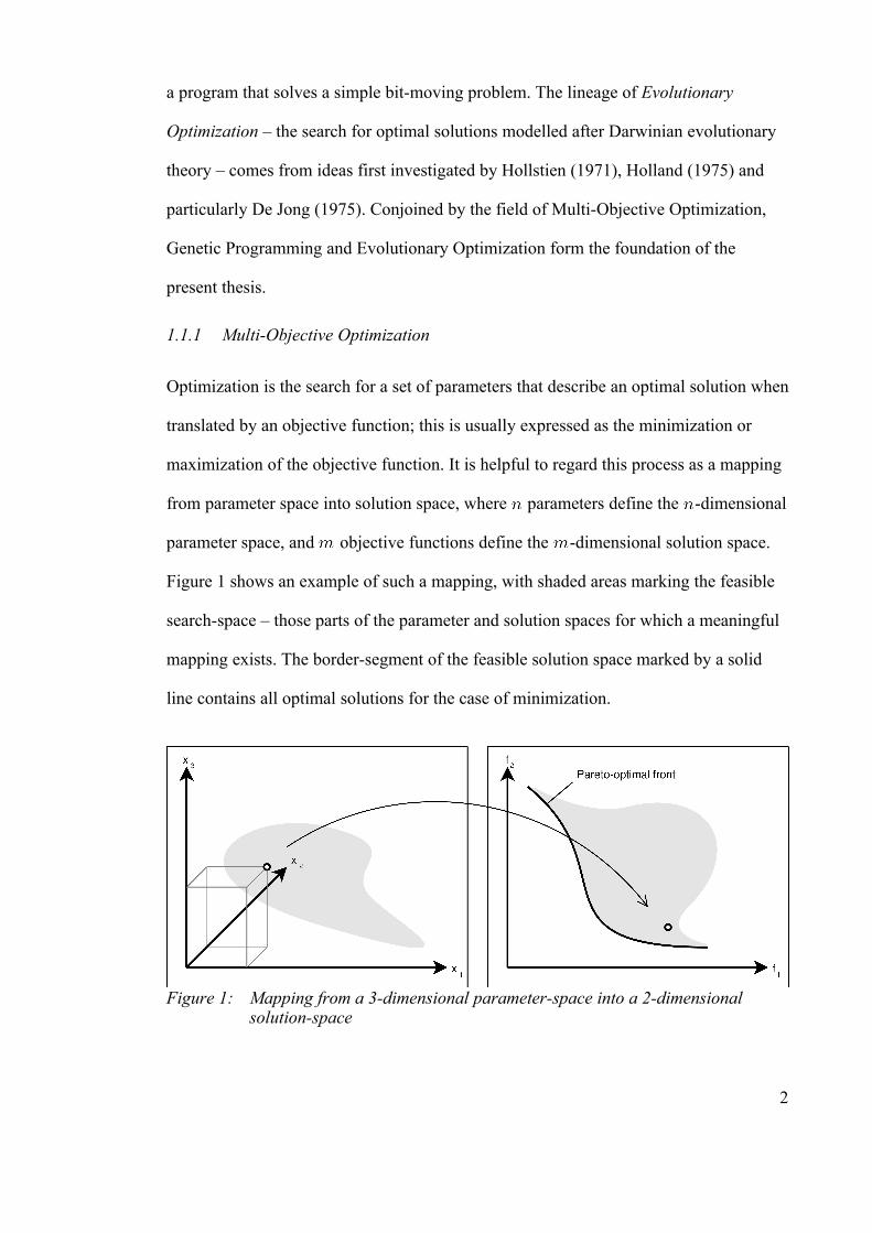
Optimization is the search for a set of parameters that describe an optimal solution when
translated by an objective function; this is usually expressed as the minimization or
maximization of the objective function. It is helpful to regard this process as a mapping
from parameter space into solution space, where parameters define the -dimensional
parameter space, and objective functions define the -dimensional solution space.
Figure 1 shows an example of such a mapping, with shaded areas marking the feasible
search-space – those parts of the parameter and solution spaces for which a meaningful
mapping exists. The border-segment of the feasible solution space marked by a solid
line contains all optimal solutions for the case of minimization.
2
Figure 1: Mapping from a 3-dimensional parameter-space into a 2-dimensional solution-space

In many real-world optimization problems, multiple objectives need to be optimized in
order to find a satisfactory solution. An optimization problem in which two or more
objective functions share at least one parameter is called a Multi-Objective
Optimization problem. In interesting cases there are two or more conflicting and often
incommensurable objectives; this leads to so-called trade-off situations in which each
objective can only be improved at the cost of degradation in one or more other
objectives. Due to the non-linear nature of Multi-Objective Optimization problems,
deceptive local trade-off solutions may exist. Such a local trade-off solution is called a
local optimum. Its counterpart, the global optimum, is also called Pareto-optimal
solution.
The field of Multi-Objective Optimization seeks to assist a (human) decision-maker in
choosing an appropriate solution (Coello Coello, 2000; Deb, 2001). A typical
classification of methods for multi-objective decision making (Hwang and Masud,
1979) describes four possible points of influence when the decision-maker's preferences
may enter the formal decision-making process:
1. No point of influence (automatic search without intervention from the decision-
maker)
2. Before the search (a priori approach)
3. During the search (progressive approach)
4. After the search (a posteriori approach)
Since the decision-maker cannot usually be expected to have a priori insight in the
exact trade-off among objective functions, it is generally considered desirable to use the
a posteriori approach and present the decision-maker with a selection of promising
solutions – an approximation set – which takes into account such trade-off behaviour.
3

The relation between two of these promising solutions is captured in the concept of
Pareto-nondomination: a solution is said to dominate another solution (also
written ) if the following conditions are both satisfied:
1. is no worse than in all objectives;
2. is better than in at least one of the objectives.
If either of the two conditions are not satisfied, then does not dominate .
Non-domination does not permit any assertions about the reversal of the relation:
simply because does not dominate , it does not necessarily follow that
dominates . On the other hand, if dominates , we can conversely say that
does not dominate . If neither solution dominates the other, the two are non-
dominated to each other. The subset of all solutions within the feasible solution space
which are not dominated by any other solution is called the
Pareto-optimal set or Pareto-optimal front. All members of the Pareto-optimal set are
thus by definition non-dominated to each other.
1.1.2 Evolutionary Algorithms
Evolutionary Algorithms leverage concepts found in Darwinian evolutionary theory to
model efficient search behaviour. Iterating over a number of generations, a population
of individual approximations is subjected to crossover and mutation operators, fitness
evaluation and reproduction.
A Fitness function reflects the quality of a set of parameters with respect to the
objectives of the search. Individual solutions are encoded into a genome (usually in
binary form or as a so-called real-value genome) and subjected to genetic operators at
the beginning of each generation. The mutation operator randomly modifies parts of the
4

genome, while the crossover operator swaps parts of two individuals' genomes. The
resulting modified genome is then used as an input to the fitness function. If the
resulting fitness is good, this heightens the probability of an individual's inclusion in the
next generation by a reproduction operator. The entire process is repeated in subsequent
generations until an exit condition is reached, usually a predefined minimal fitness level
or a maximum number of generations.
1.1.3 Evolutionary Algorithms in Multi-Objective Optimization
One of the defining properties of Evolutionary Algorithms is the fact that they are
population based and therefore operate on multiple solutions in parallel. On an intuitive
level this matches naturally with the goal of finding multiple Pareto-optimal solutions.
However, it has been shown that it is not straightforward to exploit this connection;
Evolutionary Algorithms have the tendency to converge towards a single solution
within the feasible solution space, whereas the desired result encompasses a maximally
distributed subset of the entire Pareto-optimal set (Deb, 2001).
Coello Coello (2005) describes three classes of Multi-Objective Evolutionary
Algorithms (MOEAs):
1. Aggregating functions reduce the multi-objective problem to a single objective
problem by aggregating all objective functions into one, for example with the
use of a weight or bias vector. Since such a vector must be defined before any
fitness-evaluation can take place, aggregating functions fall into the class of
a priori approaches to multi-objective decision making.
2. Population-based approaches leverage the population of an Evolutionary
Algorithm to obtain diverse solutions, without making use of the concept of
Pareto domination.
5
3. Pareto-based approaches explicitly use Pareto domination as a fitness criterion.
They can be grouped into two generations: the first generation uses fitness
sharing and niching combined with Pareto ranking to overcome the difficulties
posed by the point-convergence behaviour. The introduction of e litism marks
the beginning of the second generation. Elitism was first described in De Jong
(1975) and its application to MOEAs was suggested by Rudolph (1996). In
elitism, an archive population of non-dominated solutions is used to prevent the
loss of promising solutions due to the stochastic nature of selection and
reproduction operators.
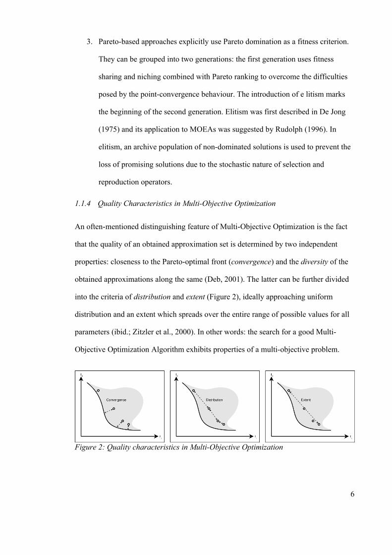
1.1.4 Quality Characteristics in Multi-Objective Optimization
An often-mentioned distinguishing feature of Multi-Objective Optimization is the fact
that the quality of an obtained approximation set is determined by two independent
properties: closeness to the Pareto-optimal front (convergence) and the diversity of the
obtained approximations along the same (Deb, 2001). The latter can be further divided
into the criteria of distribution and extent (Figure 2), ideally approaching uniform
distribution and an extent which spreads over the entire range of possible values for all
parameters (ibid.; Zitzler et al., 2000). In other words: the search for a good Multi-
Objective Optimization Algorithm exhibits properties of a multi-objective problem.
6
Figure 2: Quality characteristics in Multi-Objective Optimization
1.1.5 Genetic Programming
The related field of Genetic Programming (GP) is another type of evolutionary search.
Here, instead of binary or real-value parameters, the genome consists of an executable
program (syntax tree, linear or graph-based structures). GP can be seen as a
generalization of traditional Evolutionary Algorithms: the latter usually search for
optimal parameter-configurations for a given evaluation function specific to the problem
domain. The former can additionally search for evaluation functions, given a set of
terminals and operations specific to the problem domain.
Due to GP's close relation to traditional Evolutionary Algorithms, many concepts found
in MOEA research are applicable in GP. Rodriguez-Vazquez et al. (1997) explored the
area of Multi-Objective Genetic Programming; others have investigated the utility of the
concept of Pareto dominance in dealing with the problem of "code bloat" (De Jong et
al., 2001; Ekárt and Németh, 2001; De Jong and Pollack, 2003). In a somewhat less
obvious way the concepts of GP should be applicable to the search for new MOEAs:
since the search for a good Multi-Objective Optimization Algorithm is itself a multi-
objective problem; and since GP is designed to evolve algorithms, and MOEA-concepts
are applicable within GP; it follows that it should be feasible to search for a Multi-
Objective Evolutionary Algorithm using Multi-Objective Genetic Programming.
1.2 Searching for non-dominated Multi-Objective Evolutionary Algorithms
The aim of the presented research is to investigate how Multi-Objective Genetic
Programming (MOGP) can be used in the search for new MOEAs. Borrowing from
Turing, one could say it attempts to teach MOEA child machines to learn, employing
MOGP as a substitute teacher. The curriculum: MOEAs and evolutionary computation
in general are well-researched fields; there are many genetic operators (crossover,
7
mutation, fitness evaluation, selection and reproduction) to choose from the literature,
which can then be utilized as (high-level) building-blocks in an MOGP system.
Additionally, lower-level functions can be extracted from them and used to search new
genetic operators.
Besides defining a framework for the generation of MOEAs within an MOGP system
and proposing a selection of such high- and lower-level building blocks, the
introduction of a classification for formally incomparable approximation sets is another
contribution to knowledge by this thesis. Furthermore, it presents insights into the
idiosyncrasies of such nested evolutions and provides researchers with statistical data
concerning the trade-off behaviour between convergence and diversity. Practitioners
may find the same information helpful in selecting an MOEA for their specific problem
domain.
1.3 Overview of the Dissertation
This dissertation attempts to fulfil its aims in three phases. Based on related research, a
framework for the evolutionary generation of Multi-Objective Evolutionary Algorithms
(MOEAs) is first defined, including test problems and a combination of performance
metrics. In a second experimental part, it shows that the concepts of Genetic
Programming (GP) are indeed applicable to the domain of MOEAs: firstly by exploring
combinations of known good genetic operators, and secondly by searching for new
selection operators using a number of lower-level functions extracted from the same.
Third, the collected data and its analysis yield insights into the performance of various
genetic operators and selection mechanisms. Three interesting automatically produced
combinations of lower-level functions are presented in detail and the most promising of
them is quantitatively compared to an established MOEA.
8

1.4 Summary
From the second half of the 20th century, computer scientists have sought ways to teach
machines to learn. In the presented thesis, two areas within the field of machine learning
are of special interest: Multi-Objective Evolutionary Algorithms (MOEA), and Genetic
Programming (GP). The area of MOEAs poses many problems to the researcher,
namely the trade-off between convergence and diversity. GP profits from results found
in MOEA research, and may in turn present us with ways to tackle some of MOEAs'
foremost problems. By teaching MOEA child machines to learn with the aid of a GP
teacher, this thesis aims to explore some of these paths.
9

Chapter 2 Literature Review
2.1 Introduction
This dissertation aims to draw together the two research fields of Multi-Objective
Evolutionary Algorithms (MOEAs) and Genetic Programming (GP). The literature
review concentrates on those aspects of both fields that are necessary or beneficial
prerequisites for the empirical steps towards that aim. In the case of GP, our substitute
teacher, we need an overview of the concept and its applicability to the problem
domain, along with an indication of the greatest pitfalls to be avoided. In the case of
MOEAs, which play the role of child machines, we look at what there is to learn for
them, and how to test and rate their progress.
2.2 Genetic Programming
2.2.1 Inception and theory
First described by John R. Koza (1990), GP provides a framework for the automatic
generation of computer programs using evolutionary algorithms. Unlike traditional
evolutionary algorithms, which usually operate on parameter-vectors, GP manipulates
program structures. Subsequent research has theoretically validated key concepts,
including convergence proofs for both linear and tree-based GP (Langdon and Poli,
2002). It has also been demonstrated empirically that GP can be a valid tool in finding
new solutions to complex problems in many domains (Koza et al., 1999).
2.2.2 Code-bloat
One problem often observed in GP experiments is the so-called code-bloat: During the
course of a GP run, the average size of the individuals in a GP-population will grow
uncontrollably, leading in extreme cases to stagnation – no further evolution is possible.
10

Code-bloat is closely associated with so-called introns, arbitrarily large occurrences of
superfluous code that do not alter the result produced by an individual (Banzhaf et al.
1998). It has been shown empirically that genetic operators work most efficiently on
dense program structures with few introns; these findings were reinforced and explained
through theoretical analysis (Greene, 2005). Classic approaches in dealing with code
bloat include defining an upper limit for program size, and linearly degrading individual
fitness as program size grows. Unfortunately, the former requires a confident estimate
of the program size needed for a satisfactory solution and thus does not scale well,
whereas with the latter approach, good solutions may be lost due to the resulting
indiscriminate selection pressure.
2.2.3 Multi-Objective Genetic Programming
A promising approach to dealing with code-bloat is explored in De Jong et al. (2001),
Bleuler et al. (2001) and De Jong and Pollack (2003): it is generally an implicit goal in
GP to obtain small candidate solutions with as few introns as possible. In the Multi-
Objective GP approach (MOGP) that goal is made explicit. Various Pareto-domination-
based algorithms can then be used to address this newly defined multi-objective
problem. To preclude the problem of premature convergence, a crowding metric can be
employed as a third objective.
2.2.4 Necessary Preparations for a GP-System
Before a GP-System can be run, the following five preparatory steps need to be taken
(Koza, 1994):
1. Determine the set of terminals
2. Determine the set of primitive functions
11
3. Define the fitness measure
4. Choose the parameters for controlling the run
5. Define a method for designating a result and termination criteria.
In the experiments conducted in the course of this study, the first three of these come
from the domain of MOEAs. The following section provides background on the
possible choices.
2.3 Multi-Objective Evolutionary Optimization
In order to define a valid fitness measure for the GP-System, a deeper look at
performance comparison of MOEAs is needed: in the context of this thesis, each GP-
experiment will yield an approximation set of individual solutions , of which each
element is itself an evolutionary algorithm and, after fitness evaluation, an
associate approximation set. The fitness of should reflect how well it approximates
the Pareto-optimal set of any given multi-objective problem. In the last several years
much thought and research has gone into establishing methods that allow an objective
comparison of MOEAs. Efforts in this field can be grouped into two distinct areas:
performance metrics and test problems
2.3.1 Performance metrics
The set of solutions found by an MOEA is called the approximation set. While it is
theoretically possible for to be a subset of the Pareto-optimal set , this is usually
not the case. Performance Metrics provide an unbiased way to measure how well an
MOEA can approximate the Pareto-optimal front. The adequacy of a set of solutions is
determined by both its closeness (convergence) to the Pareto-optimal front and its
diversity (or distribution) along the same (Deb, 2001; Bosman and Thierens, 2003).
12

Zitzler et al. (2000) name the extent (or spread) as a separate third objective. In order to
obtain quantitative expressions of these objectives, many performance metrics have
been defined:
• An early metric measuring the quality of distribution of the solutions in an
approximation set is the Spacing Metric (Schott, 1995). It essentially depicts the
standard deviation from the mean distance between neighbouring members of the
approximation set and thus does not take into account the extent of the
approximation set.
• Fonseca and Fleming (1996) describe the Attainment Surface Metric. The
attainment surface is the boundary which separates all points in the solution space
that are dominated by at least one result-vector from the ones that are not. If
multiple runs of an MOEA are considered, the -attainment surface
encompasses all points that are likely to be dominated in at least of all runs.
The main limitation of this approach, as stated by the investigators themselves, is
that probability estimates for attainment can only be made for single points and not
for the entire surface.
• The Generational Distance metric (Van Veldhuizen and Lamont, 1998) measures
the average distance between an approximation set and the Pareto optimal set
. For each of the members of the approximation set, the nearest member
of the Pareto optimal set is identified and their Euclidean distance (the length
of a straight line in solution space from to ) is computed. The Generational
13

Distance is defined as the arithmetic average of these values:
• The Hypervolume Metric first described by Zitzler and Thiele (1998b) is derived
from the volume of the union of all hypercubes formed with the elements of the
approximation set and a reference point . It corresponds to the size (the
hypervolume) of that part of the solution space which comprises all points
dominated by at least one member of the approximation set.
• The Set Coverage Metric suggested ibid. calculates the proportion of solutions in
an approximation set which are strongly dominated (or covered) by any
member of another approximation .
• The Error Ratio (Van Veldhuizen, 1999) is defined as the proportion of solutions
in an approximation set which are not part of the Pareto-optimal set:
where is the number of individuals in , if the solution is part of the
Pareto optimal set and otherwise.
• The Maximum Pareto Front Error (ibid.) determines a maximum error band with
respect to the Pareto optimal front, which encompasses all members of an
approximation set. Similar to the Generational Distance, for each of the members
of the approximation set the nearest member of the Pareto optimal is identified and
their Euclidean distance calculated. The greatest of these values is the Maximum
Pareto Front Error.
14

• The Maximum Spread Metric defined by Zitzler (1999) measures the diagonal of
that hypercube which encompasses all solutions in the approximation set; this
hypercube is identified by the extreme values found in the approximation set with
respect to each objective function.
• As mentioned above, one problem associated with the Spacing Metric is the fact
that it carries no information about the obtained range of solutions. Whether the
solutions spread over a wide range or are concentrated in one small area of the
Pareto optimal front, an approximation set will have perfect spacing as long as the
solutions are distributed evenly. To alleviate this problem, the Spread Metric was
suggested by Deb et al. (2000). For each objective , the distance between
the champion solution in the Pareto optimal set and the corresponding closest
member of the approximation set is taken. The sum of these is then used as
follows:
where is the shortest distance (e.g. the Euclidean distance, others are allowed
also) between a member of the approximation set and any other member and
is the mean value of all of these distances.
• A recent Performance Metric concerned with distribution quality was suggested by
Farhang-Mehr and Azarm (2002a). To calculate the Entropy Metric, an -
dimensional approximation set is first mapped into an -dimensional space
with the aid of a procedure known as the Gram-Schmidt orthogonalization. The
Density function of the resulting density-hypersurface can then be calculated with
the aid of an influence function – a decreasing function of the distance to a point in
15

the density-hypersurface (e.g. a Gaussian function). Finally the Entropy Metric is
found by calculating the flatness of the Density function.
• A shortcoming of the Generational Distance metric is the fact that an
approximation set consisting of one single good individual has a smaller (i.e.
better) Generational Distance value than another approximation set which finds
slightly worse solutions all along the Pareto optimal front. In other words, the
distribution of the approximation set is not taken into account. By including this
information, the Reverse Generational Distance described by Bosman and
Thierens (2003) alleviates this problem. It is defined as the average Euclidean
distance of each member of the Pareto optimal set to the closest member of the
approximation set. Although Bosman and Thierens define the Reverse
Generational Distance for continuous problems as a line integration over the entire
Pareto optimal front, they suggest using a uniformly sampled set of solutions for
most practical test applications.
• Similar to the Entropy Metric, the Sparsity Measure (Deb et al., 2005) maps
solutions into a suitable hyperplane. Each projected solution is then given a
surrounding hyper-cube with a side-length defined by a parameter . The total
hyper-volume covered by all hyper-cubes created in this way, normalized by
dividing with the total hyper-volume that could be covered if none of the hyper-
cubes would overlap, is the resulting Sparsity Measure.
In the late 1990s, theoretical investigations have shown that most of the above
Performance Metrics are inadequate for the comparison of MOEAs. Hansen and
Jaszkiewicz (1998) lay the theoretical foundations for the comparison of approximation
sets by defining a set of outperformance relations. They recognized the main difficulty
16

with this approach to be that the majority of theoretically possible approximation sets
are in fact incomparable by the said outperformance relations. On this base, they then
proceeded to propose a range of comparison operators. To deal with the problem of
incomparability, comparison operators based on utility functions and other quantitative
comparison methods were proposed. Unfortunately all of these are only weakly
compatible with the outperformance relations. Knowles and Corne (2002) expanded on
this work to put known metrics in the context of the outperformance relations.
According to their results, the usefulness of most metrics must be severely doubted.
Building on the work by Hansen and Jaszkiewicz (1998), Zitzler et al. (2002) gave a
general proof of the incompleteness of unary performance metrics: there is no unary
performance metric from which it can be induced that one approximation set is better
than another. In the general case, not even a finite combination of unary performance
metrics is sufficient. It can be shown that there is no comparison method possible which
is both compatible (a sufficient condition for a binary relation) and complete (a
necessary condition for a binary relation) in respect with a binary relation stronger than
A is not worse than B.
These findings reinforce the point made earlier, that the search for good MOEAs is
itself a multi-objective problem. A useful comparison of MOEAs can only be made
with the aid of at least two independent Performance Metrics.
2.3.2 Test design
The second aspect of Performance assessment is the design of appropriate test
problems. A considerable amount of research has gone into defining scalable test
problems that can be tuned to the various difficulties that an MOEA must overcome in
order to find the Pareto optimal set. Deb (1999) identifies eight difficulties that an
17

MOEA faces. Four of those act against convergence of an MOEA towards the Pareto-
optimal front:
1. Multimodality: multi-modal problems may exhibit a very large number of local
optima, causing an MOEA to stagnate: if the variations introduced by mutation
and crossover are too small to overcome the attraction of a local optimum, they
may be rejected even though they lie closer to the global optimum.
2. Deception: a deceptive attractor may be favoured by a majority of the search
space and thus disturb the direction of search. This difficulty is similar to
multimodality, but instead of many small deceptions it poses few widespread
ones.
3. Isolated optimum: some problems exhibit a very flat fitness landscape, divulging
next to no information about the location of the optimum; the search process
stagnates due to lack of direction.
4. Collateral noise: problems with excessive variation in the solution space can
lead to misleading fitness evaluations; good building blocks for one objective
may be ignored if the solution performs poorly for other objectives.
Three more difficulties oppose diversity of the solutions:
1. Shape of the Pareto-optimal front: if the fitness of a solution is proportional to
the number of solutions it dominates, convex regions of the Pareto-optimal front
favour solutions close to the centre of the region, while non-convex regions tend
to converge towards extreme solutions.
2. Discontinuous Pareto-optimal front: due to the stochastic nature of MOEAs,
some sub-regions of an approximation set may not survive a generation. If the
18

Pareto-optimal front is not continuous, there may be no possibility to repopulate
such an extinct sub-region.
3. Non-uniform distribution of solutions along the Pareto-optimal front: If the
density of solutions along the Pareto-optimal front is not uniform, MOEAs may
naturally converge towards the denser regions.
The last difficulty is the incorporation of constraints, which may oppose both
convergence towards the Pareto-optimal front and diversity of solutions by rendering
high-fitness solutions infeasible.
After his rigorous analysis, Deb (ibid.) proceeds to define a generic two-objective
problem, for which the amount of difficulty caused by the above points can be finely
tuned, and which may be extended to an arbitrary number of objectives:
A critique of Deb's construction principles, along with a collection of different test
problems, can be found in the doctoral dissertation submitted by Van Veldhuizen
(1999). Building on Deb's work, Zitzler et al. (2000) designed one test problem for each
of the six distinct difficulties identified by Deb, four of which are used in the present
research and explained in detail below. Test problems with more than two objectives
were presented in Deb et al. (2002).
2.3.3 Algorithms and Genetic Operators
The terminal and primitive function set that are employed in the experimental phase of
this research project are assembled from distinct elements of MOEAs described in
literature. The first investigation in Evolutionary Multi-Objective Optimization was
undertaken in J. D. Schaffer's doctoral dissertation (1984). Schaffer's Vector Evaluated
19

Genetic Algorithm (VEGA) divides the population into equal parts, optimizing each
subpopulation for one single objective. Obviously this approach strongly favours those
solutions which are specialized for one single objective. It was assumed that the
application of a crossover operator would result in other solutions along the Pareto-
optimal front. However, inherent high selection pressure leads to convergence towards
individual champion solutions.
In his textbook on Genetic Algorithms, Goldberg (1989) suggested the use of a non-
dominated sorting procedure, thus introducing the concept of Pareto optimality into the
field of MOEAs. Nearly a decade after Schaffer's VEGA, Horn and Nafpliotis, and
Fonseca and Fleming independently followed Goldberg's suggestion. In Fonseca and
Fleming (1993), an individual's fitness is determined according to its rank, which is
defined as the number of other solutions in a generation which dominate it (the rank is
then augmented by one, to avoid zero-values). The described Multi-Objective Genetic
Algorithm (MOGA) also employs a niche sharing technique, scaling the individual
fitness within each rank according to their niche count. The niche count is equivalent to
the number of solutions that lie within a solution-space hypercube with a predefined
side-length . The obvious drawback to this technique is that needs to be
defined in advance, which requires a priori insights on the shape of the solution space
and may be a difficult choice depending on the problem domain.
Another approach is described in Horn and Nafpliotis (1993). The Niched Pareto
Genetic Algorithm (NPGA) introduces a way to enhance diversity within a population
of solution vectors: NPGA uses a tournament selection operator based on Pareto
dominance. Whenever there is a tie, i.e. no solution dominates the other, selection is
performed according to which solution has the lower niche count.
20

Yet another application of Pareto dominance and niching is presented in form of the
Non-dominated Sorting Genetic Algorithm (NSGA) (Srinivas and Deb, 1994). There
are two main differences to Horn and Nafpliotis' NPGA: NSGA uses non-dominated
sorting as opposed to Pareto domination tournaments and performs the niching
calculation within the resulting Pareto fronts. Also, NSGA performs the niche counts in
parameter space, as opposed to solution space. Srinivas and Deb suggest that this will
prevent the danger of differing decision-variable configurations cancelling each other
out if they result in similar result-vectors.
In a series of papers, Günter Rudolph was able to provide a formal proof for the
convergence of an MOEA towards the Pareto-optimal set in finite time (Rudolph, 1996;
Rudolph, 1998; Rudolph, 2001a; Rudolph, 2001b). Key to the successful proof is the
introduction of an elite archive (first described in De Jong, 1975), which guarantees that
the best found solutions can not be lost due to the application of genetic operators.
Although it was later shown in Hanne (1999) that elite archives of a finite size may
suffer from partial deterioration, the proof still holds for elite archives of infinite size.
The Strength Pareto Evolutionary Algorithm (SPEA), described in Zitzler and Thiele
(1998a), incorporates an elitist strategy (here the concept was taken from Ishibuchi and
Murata, 1996), a newly introduced strength fitness measure which was applied in a
tournament selection scheme, and finally the average linkage clustering method, a
parameter-less replacement for the niche count described earlier. Comparison with other
MOEAs showed however that SPEA suffers from three main weaknesses: the coarse
fitness assignment gives identical fitness to all candidate solutions that are dominated by
the same members of the elite archive – in the extreme case where the elite archive
contains only one member, all members of the population are assigned the same fitness.
Furthermore, SPEA employs its clustering algorithm only with regard to the elite
21

archive and thus fails to effectively preserve diversity in the search population. Finally,
using clustering to reduce the elite archive size may result in loss of outer solutions. In
Zitzler et al. (2001), the authors addressed these issues with the description of SPEA2.
Here, the calculation of strength as well as clustering includes the entire population,
whereas SPEA only considered members of the elite archive.
Another important example of an elitist MOEA is the successor to NSGA, the Elitist
Non-dominated Sorting Genetic Algorithm (NSGA-II). It aims to address several
problems identified with MOEAs, namely their high computational complexity, the lack
of conservation of good solutions and the guesswork associated with the definition of a
niche size or sharing parameter. The first issue is kept in check by a consequent focus
on efficiency of the utilised algorithms, in particular the sorting of candidate solutions
into Pareto fronts. The introduction of an elite archive as suggested and implemented in
several other sources addresses the second point. Thirdly, diversity is ensured using the
newly introduced crowding distance, which measures the average side-length of the
largest cuboid enclosing each candidate solution alone (Deb et al., 2000). Since outer
solutions have no nearest neighbour on one side, they are assigned an infinite cuboid
and consequentially always selected for the next generation.
The concept of elitism has its limitation: as mentioned, Hanne (1999) showed that even
elitist Pareto-based MOEAs may encounter partial deterioration over the course of two
or more generations, if the elite set is limited in size. To solve this problem of partial
deterioration and answer to the lack of formal proof of convergence for an MOEA that
ensures diversity, Laumanns et al. (2001) introduced the concept of -dominance. In
order to guarantee convergence, their algorithm needs to work on two levels. On a
coarse level, finding an -approximate set can be achieved by only replacing a solution
from the elite archive if it is -dominated (in other words if it is dominated by more than
22

a small value ). Once an algorithm has found an approximation within -vicinity, this
coarse-level strategy obviously prevents an algorithm from finding the true Pareto-
optimal set; a second, finer level is needed: If a solution dominates an elite solution by
less than , but lies within the coarse-level box with side-lengths , it may be replaced –
thus maintaining the possibility of definitive convergence.
There are a number of Multi-Objective Algorithms inspired by MOEAs which depart
from the classic model of evolution and its operators, either by adding additional local
search algorithms or by completely replacing the genetic operators. The inclusion of
these lies outside of the scope of this thesis. Three are mentioned here in order to
establish what lies beyond the fence.
The Entropy-based Multi-Objective Genetic Algorithm (E-MOGA) developed by
Farhang Mehr and Azarm (2002b) adds a local search component based on the ideal gas
model. A multi-objective optimizer built on the principles of Particle-Swarm
Optimization is presented by Hu and Eberhart (2002). Hernández-Díaz et al. (2006)
suggested an MOEA based on differential evolution combined with a local search using
recent research on Rough Sets.
2.4 Research question
The presented research draws together the two existing fields of MOEAs and GP. It
explores the concept of utilizing GP in the search for an MOEA with good convergence
and distribution characteristics. Based on the reviewed literature, in particular taking in
account the breadth of applications of GP and the well-researched fundamentals of
MOEAs, I pose the following two Hypotheses:
1. It is feasible for a (Multi-Objective) Genetic Programming Algorithm to find an
MOEA that has similar or better convergence and distribution properties than
23

known “good” MOEAs if the search is performed using High-Level building-
blocks – such as Selection-, Crossover- and Mutation-Operators described in the
literature.
2. It is very improbable that an MOGP System can find new genetic operators and
selection mechanisms, although it is possible to build a GP-System that searches
for such operators.
2.5 Summary
The current body of knowledge relevant to the proposed project is roughly divided in
two areas. The first area is concerned with Genetic Programming, a form of
Evolutionary Computation which manipulates programs instead of configurations.
Researchers have discussed problems related to the uncontrollable growth of GP
individuals, which can be alleviated by allowing multiple objectives, and making a
small program size one of them. Among the five preparatory steps for a GP experiment,
three (in the context of this research project) fall into the domain of Multi-Objective
Evolutionary algorithms. First, a fitness measure for GP must be chosen from one of the
many MOEA-performance metrics. There is however some uncertainty concerning the
theoretic validity of the available metrics and more thought needs to go into the
validation of any selection. For both the second and third steps – selection of terminal
and primitive function sets – high-level operators can be chosen from a wealth of
MOEAs. Building on this foundation, the hypothesis is posed, that the attempted nested
evolution can yield useful results.
24

Chapter 3 Research Methods
3.1 Introduction
In pursuit of answers to the research question defined in the preceding chapter,
controlled experiments will be conducted to explore the following partial questions:
• Can GP find a good MOEA by pure recombination of known genetic operators and
selection methods?
• Can GP define new selection methods, if given appropriate building blocks, and
are they of similar quality as methods taken from the literature?
• How well do the best of these automatically generated MOEAs perform in more
complex test problems, when compared to known good MOEAs?
These experiments are based on a Multi-Objective Genetic Programming system,
running an implementation of NSGA-II. But which are the objectives? As has been
discussed in the literature review, minimization of program size has been successfully
employed to control code-bloat and figure as an objective throughout the experiments.
To determine the rest of the objectives the following needs to be done: a Performance
Metric or a combination thereof needs to be selected with care; this then needs to be
applied to one or more test functions. The combination of these will result in a number
of measurements that will serve as the remaining objective functions.
3.2 The Open BEAGLE Framework
In order to run the proposed experiments, a framework for Evolutionary Computation is
needed. The concomitant requirements include support for both Multi-Objective
Evolutionary Algorithms and Genetic Programming, high computational efficiency, and
25

provisions for the comprehensive collection of data. Additionally, ease of configuration
and code reuse are criteria towards the selection of a framework. The selected Open
BEAGLE Framework (Gagné and Parizeau, 2006) includes all of these features; its GP
implementation is tree-based and provides genetic operators that can perform mutation
and crossover safely on populations with multiple data types.
3.3 NSGA-II
The Open BEAGLE Framework provides an implementation of NSGA-II, as described
in Deb et al. (2000). First, an initial population of tree-based genomes is generated, the
individual fitness evaluated and non-dominated solutions are inserted into an
unbounded elite archive. A temporary population twice the size of the parent population
is then generated by combining the parent population with an offspring population
generated by applying five GP-operators:
• The crossover operator exchanges sub-trees between two individuals. In contrast to
the mutation operators which all result in only one offspring, here two offspring
solutions are copied to the temporary population.
• The standard mutation operator replaces a sub-tree with a newly generated one.
• The shrink mutation operator deletes a sub-tree from a solution.
• The swap mutation operator replaces a node in the tree with another one from the
set of primitives
• The sub-tree swap mutation operator exchanges two sub-trees within an individual
The resulting temporary population is then sorted into non-dominated fronts: first, all
individuals that are not dominated by any others are identified, and removed from the
26

population. The same is done for the remaining individuals recursively, until there are
no individuals left and the population is completely sorted.
The selection procedure starts with the first non-dominated front. If it is smaller than the
configured population size, all members are copied into the next generation; the same is
then done with the next non-dominated front. This step is repeated until the population
is full. If there are superfluous members in the last included non-dominated front, those
members are selected which have the greatest crowding distance: for each candidate
individual, the two nearest neighbours in the non-dominated front are found for each
objective. These form a cuboid, the average side-length of which is the crowding
distance.
Finally, the elite archive is updated, considering only individuals in the first non-
dominated front.
3.4 Tree depth instead of program size
In the tree-like genome employed throughout the experiments, program size can be seen
as equivalent to the number of nodes in a tree. Preliminary experiments showed
however, that this leads to an unfair advantage inversely proportional to the number of
arguments of an operator. Using the depth of the tree instead provides a similar pressure
against code-bloat and did not exhibit such a bias; this configuration was therefore used
in the remainder of the experiments.
3.5 Selection of a Performance Metric: the Reverse Generational Distance
The usefulness of performance metrics for the comparison of approximation sets has
been severely doubted. Great care must therefore be taken in choosing such metrics and
the validation of that choice.
27

3.5.1 Dominance Relations
In preparation of their investigation into performance metrics, Zitzler et al. (2002)
define a set of dominance relations used to assess the utility of a performance metric:
In a -dimensional solution space we define the two arbitrary approximation vectors
and : . The following relations are then
defined:
• strictly dominates , or , if is better than in all objectives
• dominates , or , if is better than in at least one objective, and
not worse in any objective
• weakly dominates , or , if is not worse than in any objective
• and are incomparable, or , if neither objective vector weakly
dominates the other
The formal definition of an approximation set is then given as follows; a set is
called an approximation set, if each of its members is incomparable (or non-dominated)
to all other members: . The set of all approximation sets
is called .
After these definitions, the objective-vector relations are used to define relations
between two approximation sets :
• strictly dominates , or , if every objective vector in is strictly
dominated by at least one objective vector in
• dominates , or , if every objective vector in is dominated by at
least one objective vector in
28
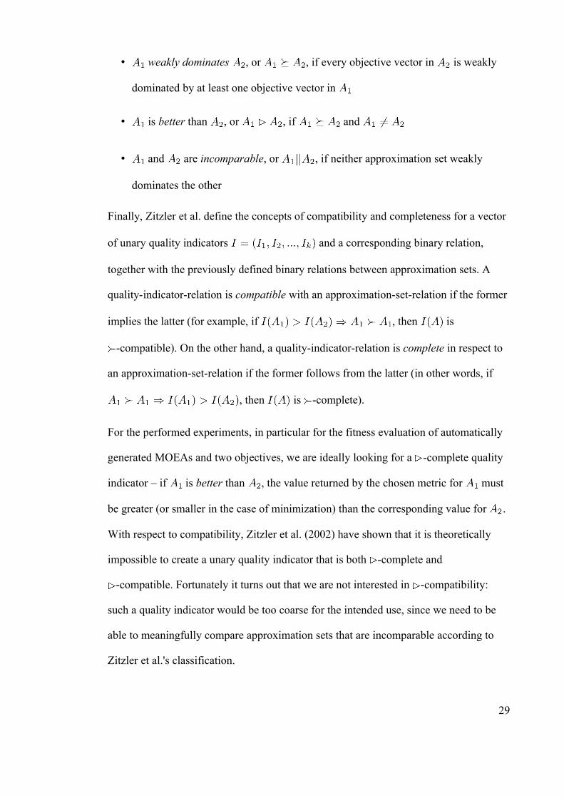
• weakly dominates , or , if every objective vector in is weakly
dominated by at least one objective vector in
• is better than , or , if and
• and are incomparable, or , if neither approximation set weakly
dominates the other
Finally, Zitzler et al. define the concepts of compatibility and completeness for a vector
of unary quality indicators and a corresponding binary relation,
together with the previously defined binary relations between approximation sets. A
quality-indicator-relation is compatible with an approximation-set-relation if the former
implies the latter (for example, if , then is
-compatible). On the other hand, a quality-indicator-relation is complete in respect to
an approximation-set-relation if the former follows from the latter (in other words, if
, then is -complete).
For the performed experiments, in particular for the fitness evaluation of automatically
generated MOEAs and two objectives, we are ideally looking for a -complete quality
indicator – if is better than , the value returned by the chosen metric for must
be greater (or smaller in the case of minimization) than the corresponding value for .
With respect to compatibility, Zitzler et al. (2002) have shown that it is theoretically
impossible to create a unary quality indicator that is both -complete and
-compatible. Fortunately it turns out that we are not interested in -compatibility:
such a quality indicator would be too coarse for the intended use, since we need to be
able to meaningfully compare approximation sets that are incomparable according to
Zitzler et al.'s classification.
29
3.5.2 Grades of comparability
I therefore propose the following informal classification for incomparable
approximation sets:
• Distribution-comparable: let and be two approximation sets such that
, in other words the union of and is itself a
different, larger approximation set (and all its elements are non-dominated to each
other). In this case that approximation set is preferable which has the better overall
distribution. Note that in this class it is still possible to have comparison-draws for
different approximation sets, for example two sets that both include a dense cluster
of solutions in different locations along the Pareto optimal front. However the
author sees no reason why such a comparison should not yield identical quality
indicator values, since without preference-input from the decision maker none can
be said to be preferable to the other.
• Convergence-comparable: let and be two approximation sets and , ,
, four subsets of and , with , and
. Here, most known convergence-based unary quality
indicators will provide a result that favours the approximation set which has the
greater proportion of good solutions. However, draws are possible, and it is easy to
construe situations where such a quality indicator will favour an approximation set
with a few perfect and many bad solutions over one with consistently good
solutions. To alleviate this last problem, the standard deviation of a convergence-
based metric can be used instead. This is an arbitrary choice to emphasize good
overall convergence over a few champion solutions – in the real-world case, where
a decision-maker chooses one solution from the obtained approximation set, it is
30

important to minimize the probability of the chosen solution being an outlier far
from the Pareto-optimal front; favouring approximation sets with uniform
convergence properties therefore raises the confidence in any chosen solution.
3.5.3 Reverse Generational Distance
As stated above, we are looking for a -complete quality indicator, which – instead of
also being -compatible – yields finer-grained information about the convergence and
distribution qualities of incomparable approximation sets. The Reverse Generational
Distance (RGD) – described in greater detail in the literature review – suggested by
Bosman and Thierens (2003) is such an indicator. It is chosen because it includes
information about the spread and distribution along the Pareto optimal front as well as
convergence towards the Pareto optimal front. One problem associated with this metric
is however that it requires careful definition of a uniform and sufficiently large set of
members of the Pareto optimal front. If is smaller than the approximation set ,
some members of will be ignored in the fitness calculation. The RGD denotes the
average closeness of an approximation set to the Pareto optimal front. As suggested
above, the standard deviation from this metric will serve to favour individuals with
good uniform convergence.
3.6 Test Problems
The inclusion of two separate Performance metrics into the objectives of our experiment
poses a problem: to prevent building an MOEA specialised for one single problem, at
least two test problems must be included in the GP-objectives. The combination of these
with two Performance measurements, together with the above mentioned minimization
of program size, results in a minimum of 5 objectives. In this scenario only the most
basic test problems can be incorporated. This is a problem for two reasons: on one hand
31

the presentation of results is difficult for more than 3 objectives. On the other hand it
has been observed that too many objectives may lead to stagnation of convergence
(Coello Coello, 2005). For those two reasons the decision was taken to combine the
performance measurements of all test problems. This leaves us free to explore four test
problems defined by Zitzler et al. (2000). All of these follow the construction principle
for two-objective problems defined by Deb (1999):
• The simplest problem, ZDT1, is a 30-variable problem with a continuous convex
Pareto optimal front:
The Pareto optimal front is found for and for .
The set of Pareto optimal solutions needed for the RGD-Metric can thus be
formed from uniform subdivisions of the value-range of .
• ZDT2 complements ZDT1 in that it is the non-convex counterpart:
The calculations of the Pareto optimal front and of are as in ZDT1.
• ZDT3 exercises the difficulty of a discontinuous Pareto optimal front:
32

Here, can be formed with relative ease by travelling along uniform subdivisions
of the value-range of in increasing order, and selecting each point that results in
a new optimum for . Like in the other test problems, the remaining optimal
parameters are for .
• ZDT4 has many local Pareto optimal fronts, making convergence difficult
The calculations of the Pareto optimal front and of are as in ZDT1.
3.7 Wilcoxon rank-sum test
The result of the data collection phase is a number of populations (and in particular their
elite archive) of tree-like genomes, assembled from predefined building blocks. For
each building block we can examine how it contributes to either objective by taking two
samples: one containing the elite archive, the other comprised of all individuals of the
elite archive that contain the specified building block. The distributions of the two
samples can now be compared with respect to each objective. Since the elite archive is
the result of an evolutionary process, we must assume that the distribution of either
sample is non-normal; therefore we do not have sufficient information about the
parameters of the samples' probability distributions to employ a parametric test like
Student's t-test. The Wilcoxon rank-sum test is used instead – a non-parametric test that
33
can compare the medians of two independent samples (Rinne, 2003; R Development
Core Team, 2006).
To determine whether an operator contributes to good convergence properties, all
individuals of an elite set that contain the operator in question are selected into the first
statistical sample of size . The second sample comprises the entire elite set with
individuals. The null-hypothesis assumes that the distributions of and are
identical, while the alternative hypothesis states that is stochastically smaller than
. The individuals in the two samples are now ranked according to their performance
measurements, and the sum of the ranks of the individuals in is calculated (ties
are resolved by averaging the respective ranks). is rejected with confidence if
. The critical value can be taken from statistical tables. This
use of the Wilcoxon rank-sum test depends on the assumption that and can be
regarded as independent samples.
3.8 Summary
The presented research concentrates on controlled experiments in the overlapping
domains of GP and MOEAs. The foundation for the experiments is provided by the
Open BEAGLE framework, with an NSGA-II algorithm as the main loop. The first
objective in this MOGP is the minimization of tree depth. By using the Reverse
Generational Distance metric in conjunction with its Standard Deviation as the second
and third objectives, an arbitrary choice is made to emphasise uniform convergence
over a few champion solutions. This choice is justified by two newly introduced classes
of incomparable approximation sets: distribution-comparable and convergence-
comparable approximation sets. It also leads to the necessity of a priori knowledge of
many points in the Pareto Optimal set. In order to avoid too many objectives, the fitness
34

measurements are averaged between all four performed test problems. The resulting
populations are then analysed using the Wilcoxon rank-sum test.
35

Chapter 4 Data Collection
4.1 Introduction
There are a wealth of diverse components described in literature, of which many
combinations can be made into a working Multi-Objective Evolutionary Algorithm
(MOEA). Putting the framework developed in the previous chapter into practice, the
first experiment defines the function and terminal sets for high-level operators and
explores the question whether there is an ideal combination, and whether we already
know it. The second experiment searches for a new selection operator using lower-level
functions. Appendix B, submitted on a separate CD, contains the developed source code
and collected data.
4.2 Experiment 1: High-level Operators
A Multi-Objective GP-System built on the base of NSGA-II forms the core of this
experiment. The objectives comprise the minimization of tree depth (in order to
preclude code-bloat), and a combination of the Reverse Generational Distance (Bosman
and Thierens, 2003) and its standard deviation taken on single runs of four test problems
ZDT1-4 (Zitzler et al., 2000).
4.2.1 Function set
The utilized function set consists of evolutionary operators from the literature. In order
to ensure a representative sample of subjects, the predefined functions span the range
from Schaffer's Vector Evaluated Genetic Algorithm (VEGA) to SPEA2. Each MOEA
described in the Literature Review was disassembled into building blocks, which can be
grouped into functional families. The collection of all these building blocks make up the
function set (Table 1). A tree genome then corresponds to the operations executed in the
36
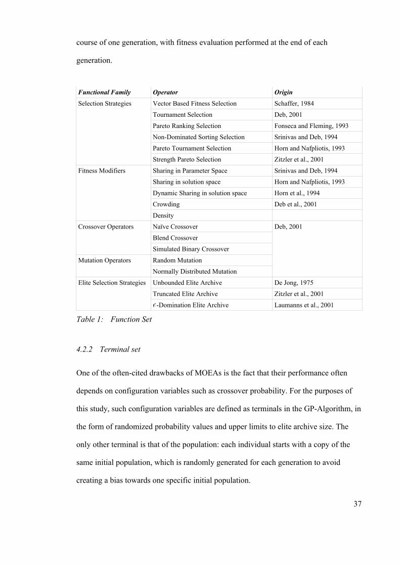
course of one generation, with fitness evaluation performed at the end of each
generation.
Functional Family Operator Origin
Selection Strategies Vector Based Fitness Selection Schaffer, 1984
Tournament Selection Deb, 2001
Pareto Ranking Selection Fonseca and Fleming, 1993
Non-Dominated Sorting Selection Srinivas and Deb, 1994
Pareto Tournament Selection Horn and Nafpliotis, 1993
Strength Pareto Selection Zitzler et al., 2001
Fitness Modifiers Sharing in Parameter Space Srinivas and Deb, 1994
Sharing in solution space Horn and Nafpliotis, 1993
Dynamic Sharing in solution space Horn et al., 1994
Crowding Deb et al., 2001
Density
Crossover Operators Naïve Crossover
Blend Crossover
Simulated Binary Crossover
Mutation Operators Random Mutation
Normally Distributed Mutation
Deb, 2001
Elite Selection Strategies Unbounded Elite Archive De Jong, 1975
Truncated Elite Archive Zitzler et al., 2001
-Domination Elite Archive Laumanns et al., 2001
Table 1: Function Set
4.2.2 Terminal set
One of the often-cited drawbacks of MOEAs is the fact that their performance often
depends on configuration variables such as crossover probability. For the purposes of
this study, such configuration variables are defined as terminals in the GP-Algorithm, in
the form of randomized probability values and upper limits to elite archive size. The
only other terminal is that of the population: each individual starts with a copy of the
same initial population, which is randomly generated for each generation to avoid
creating a bias towards one specific initial population.
37
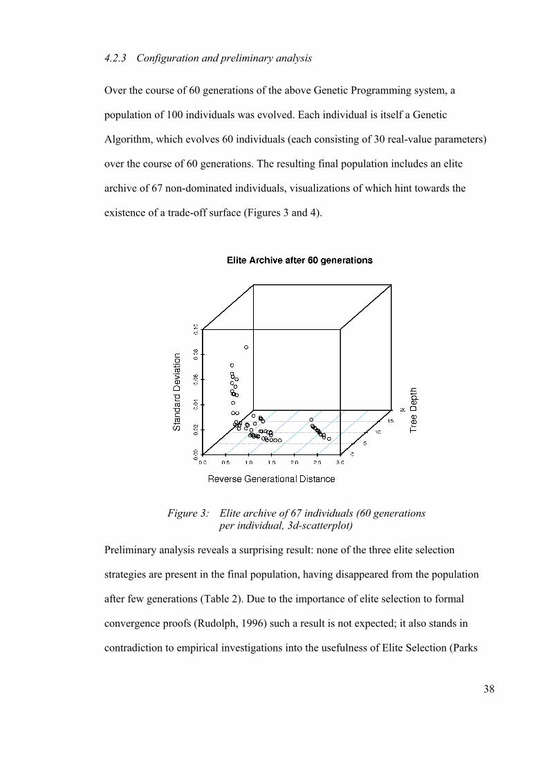
4.2.3 Configuration and preliminary analysis
Over the course of 60 generations of the above Genetic Programming system, a
population of 100 individuals was evolved. Each individual is itself a Genetic
Algorithm, which evolves 60 individuals (each consisting of 30 real-value parameters)
over the course of 60 generations. The resulting final population includes an elite
archive of 67 non-dominated individuals, visualizations of which hint towards the
existence of a trade-off surface (Figures 3 and 4).
Preliminary analysis reveals a surprising result: none of the three elite selection
strategies are present in the final population, having disappeared from the population
after few generations (Table 2). Due to the importance of elite selection to formal
convergence proofs (Rudolph, 1996) such a result is not expected; it also stands in
contradiction to empirical investigations into the usefulness of Elite Selection (Parks
38
Figure 3: Elite archive of 67 individuals (60 generations per individual, 3d-scatterplot)
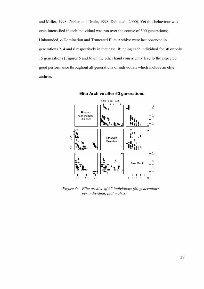
and Miller, 1998; Zitzler and Thiele, 1998; Deb et al., 2000). Yet this behaviour was
even intensified if each individual was run over the course of 300 generations;
Unbounded, -Domination and Truncated Elite Archive were last observed in
generations 2, 4 and 6 respectively in that case. Running each individual for 30 or only
15 generations (Figures 5 and 6) on the other hand consistently lead to the expected
good performance throughout all generations of individuals which include an elite
archive.
39
Figure 4: Elite archive of 67 individuals (60 generations per individual, plot matrix)
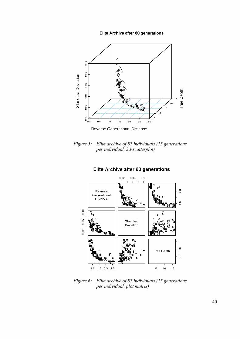
40
Figure 5: Elite archive of 87 individuals (15 generations per individual, 3d-scatterplot)
Figure 6: Elite archive of 87 individuals (15 generations per individual, plot matrix)

Operator Generation
Truncated Elite Archive 5
-Domination Elite Archive 7
Unbounded Elite Archive 16
Table 2: Last occurrence of Elite Selection Strategies in individuals with 60 generations
A possible explanation for the observed pattern is, that although the inclusion of an elite
archive is beneficial for an MOEA, it competes with the disadvantage of introducing an
additional depth-level into the individual's genome. As the number of allowed
generations increases, an individual has ample time to find good solutions – the relative
importance of the elite archive decreases and is not enough to counterbalance the
disadvantage in the objective of program size.
4.3 Experiment 2: Lower-level Selection
4.3.1 Function set
The selection strategies and fitness modifiers included in the function set in Table 1 are
themselves built upon similar building blocks. A variation of the initial setting is
therefore to replace the former with a selection of the latter in the primitive set and let
the GP-System search for new combinations of these. These lower-level building blocks
are used in combination with a Skeleton Selection Strategy to enable GP to explore that
search space (Table 3).
4.3.2 Terminal set
Initially, no alterations were made to the terminal set. Early results showed however,
that a randomized configuration variable (denoting the size-limit of the Truncated Elite
Archive) in combination with the newly introduced Skeleton Selection Strategy led to a
highly deceptive local optimum: an individual that includes such a combination has a
41
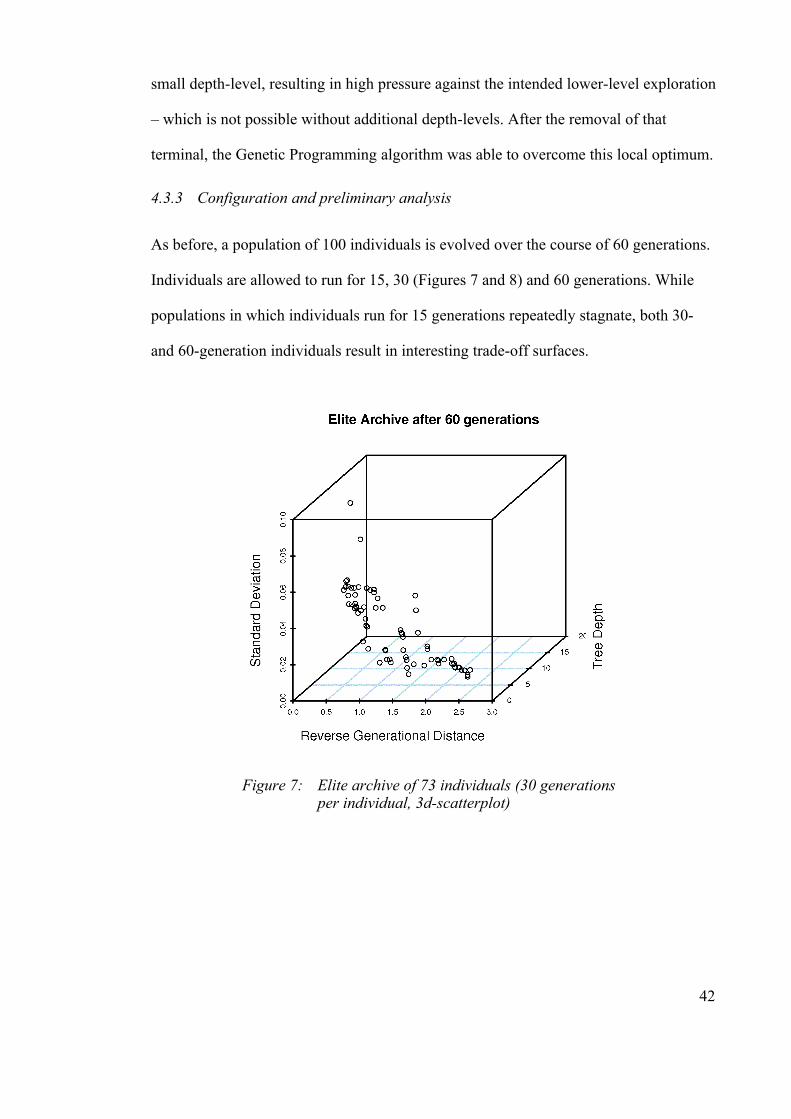
small depth-level, resulting in high pressure against the intended lower-level exploration
– which is not possible without additional depth-levels. After the removal of that
terminal, the Genetic Programming algorithm was able to overcome this local optimum.
4.3.3 Configuration and preliminary analysis
As before, a population of 100 individuals is evolved over the course of 60 generations.
Individuals are allowed to run for 15, 30 (Figures 7 and 8) and 60 generations. While
populations in which individuals run for 15 generations repeatedly stagnate, both 30-
and 60-generation individuals result in interesting trade-off surfaces.
42
Figure 7: Elite archive of 73 individuals (30 generations per individual, 3d-scatterplot)

Lower-Level Operator Description
Skeleton Selection Strategy Creates a new population by calling its subtree once for each individual; updating the new population with an individual from the previous population at the position returned by the subtree.
Random Individual Returns the position of a random Individual in the current population.
Select Lesser Selects from two positions of Individuals in the current population that one, for which a subtree of metric calculations returns the lesser value.
Select Greater Selects from two positions of Individuals in the current population that one, for which a subtree of metric calculations returns the greater value.
Least Objective Distance Calculates the Euclidean distance in solution space between an individual and all others in the current population, and returns the least of these.
Average Objective Distance Calculates the Euclidean distance in solution space between an individual and all others in the current population, and returns the arithmetic average of these.
Greatest Objective Distance Calculates the Euclidean distance in solution space between an individual and all others in the current population, and returns the greatest of these.
Least Parameter Distance Calculates the Euclidean distance in parameter space between an individual and all others in the current population, and returns the least of these.
Average Parameter Distance Calculates the Euclidean distance in parameter space between an individual and all others in the current population, and returns the arithmetic average of these.
Greatest Parameter Distance Calculates the Euclidean distance in parameter space between an individual and all others in the current population, and returns the greatest of these.
Dominator Count Counts the number of individuals in the current population that dominate an individual. Equivalent to Pareto ranking.
Dominated Count Counts the number of individuals in the current population that are dominated by an individual.
Add
Subtract
Multiply
Divide
Absolute
Sine
Cosine
Arithmetic operations. These are used to combine metrics.
Table 3: Lower-level building-blocks
43

4.4 Summary
Controlled experiments were conducted first to explore possible recombinations of
known good genetic operators. An interesting preliminary result is the fact that Elite
selection strategies disappear from the population when individual solutions are run for
a sufficient number of generations. Preliminary runs of a subsequent experiment
exploring the combination of lower-level functions into a new selection operator
displayed a similar idiosyncrasy: two unrelated primitives (the newly introduced
Skeleton Selection Strategy and a randomized configuration variable) formed a highly
deceptive local optimum. The removal of the latter helped circumvent that problem.
44
Figure 8: Elite archive of 73 individuals (30 generations per individual, plot matrix)
Chapter 5 Results
5.1 Introduction
The results of the two previous experiments need to be treated differently. The findings
of the first experiment are grouped by functional families. In each family, a one-sided
Wilcoxon rank-sum test is used to compare the distribution of solutions with each
operator. For each sample of individuals, the null-hypothesis ( ) states that the
distribution of the samples is the same. The alternative hypothesis asserts that the
distribution of one sample is statistically smaller than the other.
In the second experiment, promising solutions are of interest. Some sub-trees appear in
multiple good solutions. These are presented in detail and potential reasons for their
success are given. Finally, testing the validity of the results, one of the resulting
champion solutions is run against NSGA-II.
5.2 Performance of high-level genetic operators
A first glance at the development of the Reverse Generational Distance over the course
of 60 generations shows that there is indeed convergence towards a good MOEA. Both
the best (Figure 9) and the average values (Figure 10) improve continuously. As is to be
expected, performance of the best individual of each experiment appears to coincide
with the number of generations it is allowed to run – champion solutions that ran for 60
generations perform better than champions that ran for only 15 generations. Of
particular interest is an exception to this rule: one champion running for 30 generations
outperforms all but the best 60-generation individual. A closer look (Figure 12) reveals
the nature of this individual's advantage: repetition. By including no less than 5
selection- and 4 elite archiving operators, this individual has learned not to find an ideal
45
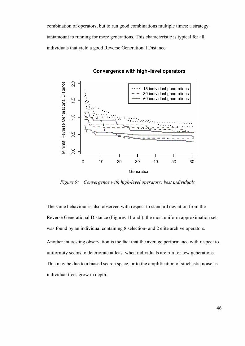
combination of operators, but to run good combinations multiple times; a strategy
tantamount to running for more generations. This characteristic is typical for all
individuals that yield a good Reverse Generational Distance.
The same behaviour is also observed with respect to standard deviation from the
Reverse Generational Distance (Figures 11 and ): the most uniform approximation set
was found by an individual containing 8 selection- and 2 elite archive operators.
Another interesting observation is the fact that the average performance with respect to
uniformity seems to deteriorate at least when individuals are run for few generations.
This may be due to a biased search space, or to the amplification of stochastic noise as
individual trees grow in depth.
46
Figure 9: Convergence with high-level operators: best individuals
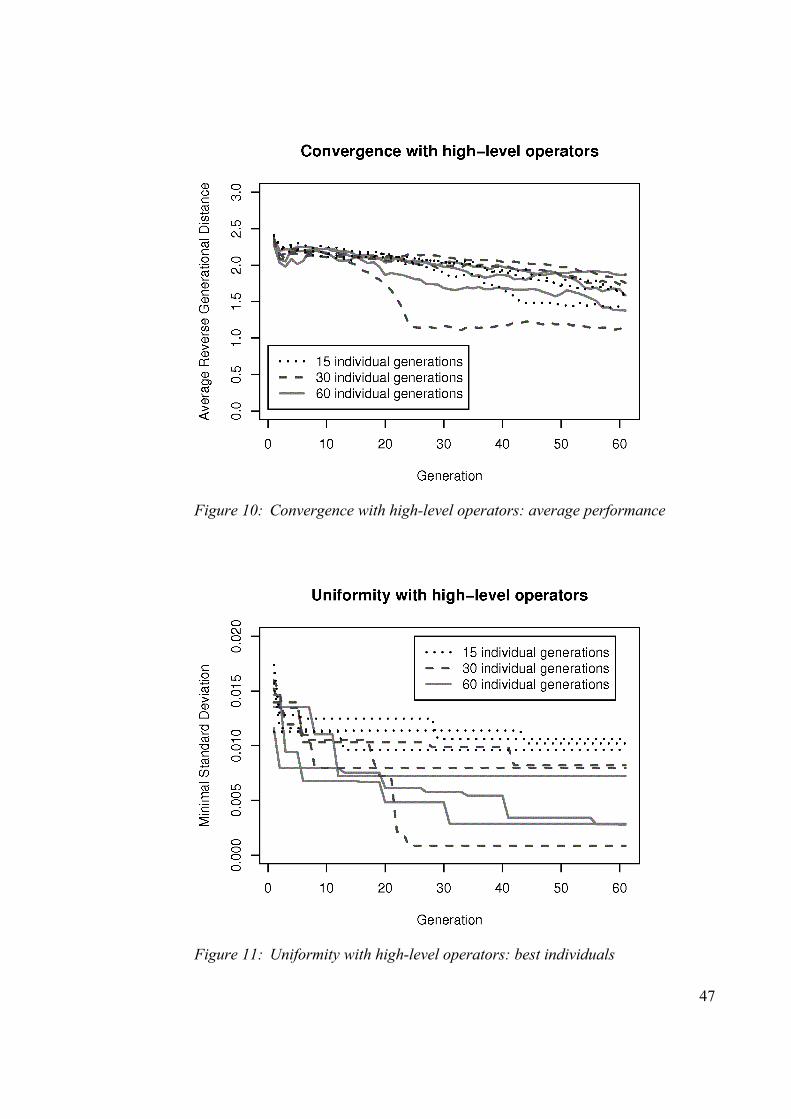
47
Figure 10: Convergence with high-level operators: average performance
Figure 11: Uniformity with high-level operators: best individuals
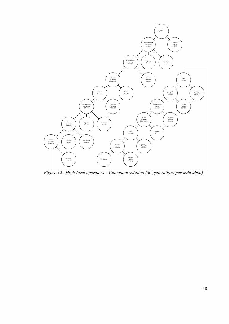
48
Figure 12: High-level operators – Champion solution (30 generations per individual)
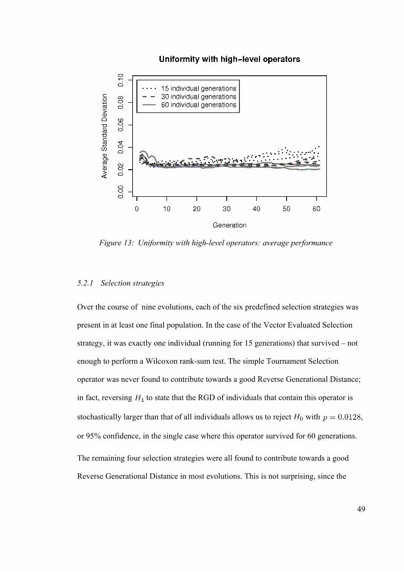
5.2.1 Selection strategies
Over the course of nine evolutions, each of the six predefined selection strategies was
present in at least one final population. In the case of the Vector Evaluated Selection
strategy, it was exactly one individual (running for 15 generations) that survived – not
enough to perform a Wilcoxon rank-sum test. The simple Tournament Selection
operator was never found to contribute towards a good Reverse Generational Distance;
in fact, reversing to state that the RGD of individuals that contain this operator is
stochastically larger than that of all individuals allows us to reject with ,
or 95% confidence, in the single case where this operator survived for 60 generations.
The remaining four selection strategies were all found to contribute towards a good
Reverse Generational Distance in most evolutions. This is not surprising, since the
49
Figure 13: Uniformity with high-level operators: average performance

population usually also contains individuals that have no selection operator whatsoever
– naturally such an individual will not converge any more than a repeated creation of
random parameters. However, there are exceptions. Table 4 shows the probability for
in the one-sided Wilcoxon rank-sum test for each evolution where a selection
strategy is present. Where can be rejected with 95% or even 99% confidence, the
upper bound of the confidence interval is given.
Further than that, no reproducible and significant hierarchy could be found; the Strength
Pareto selection operator is the only one present in all final populations, which leads to
the assumption that individuals containing it should perform consistently better than
other selection strategies. Pairwise statistical comparison does not confirm that
assumption. In fact when present in the final population, each of the three other
Selection Strategies seems to perform clearly better than Strength Pareto in two
instances – but worse in the two remaining direct comparisons (Table 5).
50
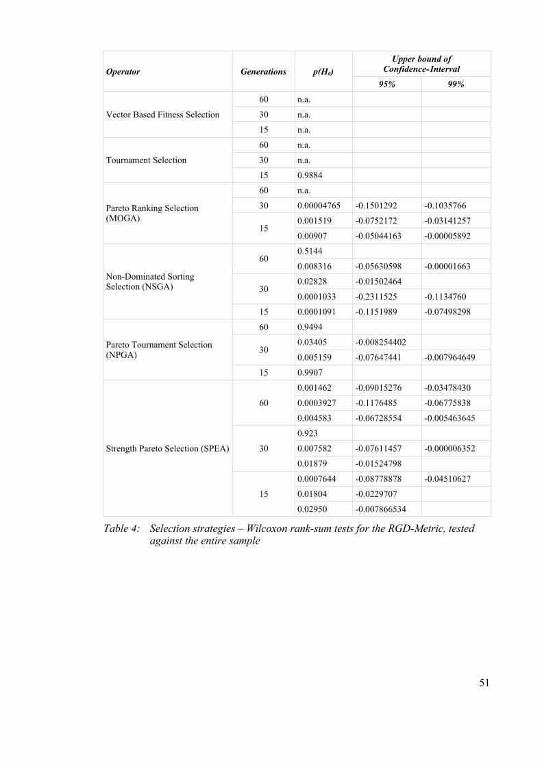
Operator Generations p(H0)
Upper bound of Confidence-Interval
95% 99%
Vector Based Fitness Selection
60 n.a.
30 n.a.
15 n.a.
Tournament Selection
60 n.a.
30 n.a.
15 0.9884
Pareto Ranking Selection (MOGA)
60 n.a.
30 0.00004765 -0.1501292 -0.1035766
150.001519 -0.0752172 -0.03141257
0.00907 -0.05044163 -0.00005892
Non-Dominated Sorting Selection (NSGA)
600.5144
0.008316 -0.05630598 -0.00001663
300.02828 -0.01502464
0.0001033 -0.2311525 -0.1134760
15 0.0001091 -0.1151989 -0.07498298
Pareto Tournament Selection (NPGA)
60 0.9494
300.03405 -0.008254402
0.005159 -0.07647441 -0.007964649
15 0.9907
Strength Pareto Selection (SPEA)
60
0.001462 -0.09015276 -0.03478430
0.0003927 -0.1176485 -0.06775838
0.004583 -0.06728554 -0.005463645
30
0.923
0.007582 -0.07611457 -0.000006352
0.01879 -0.01524798
15
0.0007644 -0.08778878 -0.04510627
0.01804 -0.0229707
0.02950 -0.007866534
Table 4: Selection strategies – Wilcoxon rank-sum tests for the RGD-Metric, tested against the entire sample
51
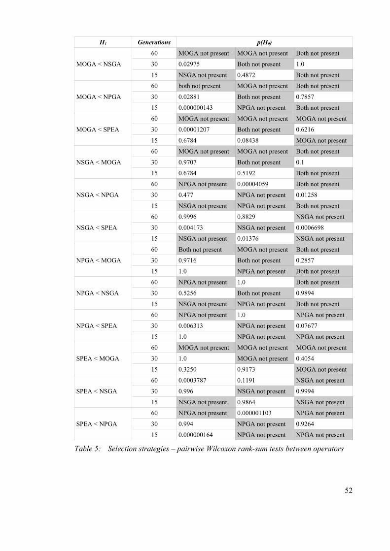
H1 Generations p(H0)
MOGA < NSGA
60 MOGA not present MOGA not present Both not present
30 0.02975 Both not present 1.0
15 NSGA not present 0.4872 Both not present
MOGA < NPGA
60 both not present MOGA not present Both not present
30 0.02881 Both not present 0.7857
15 0.000000143 NPGA not present Both not present
MOGA < SPEA
60 MOGA not present MOGA not present MOGA not present
30 0.00001207 Both not present 0.6216
15 0.6784 0.08438 MOGA not present
NSGA < MOGA
60 MOGA not present MOGA not present Both not present
30 0.9707 Both not present 0.1
15 0.6784 0.5192 Both not present
NSGA < NPGA
60 NPGA not present 0.00004059 Both not present
30 0.477 NPGA not present 0.01258
15 NSGA not present NPGA not present Both not present
NSGA < SPEA
60 0.9996 0.8829 NSGA not present
30 0.004173 NSGA not present 0.0006698
15 NSGA not present 0.01376 NSGA not present
NPGA < MOGA
60 Both not present MOGA not present Both not present
30 0.9716 Both not present 0.2857
15 1.0 NPGA not present Both not present
NPGA < NSGA
60 NPGA not present 1.0 Both not present
30 0.5256 Both not present 0.9894
15 NSGA not present NPGA not present Both not present
NPGA < SPEA
60 NPGA not present 1.0 NPGA not present
30 0.006313 NPGA not present 0.07677
15 1.0 NPGA not present NPGA not present
SPEA < MOGA
60 MOGA not present MOGA not present MOGA not present
30 1.0 MOGA not present 0.4054
15 0.3250 0.9173 MOGA not present
SPEA < NSGA
60 0.0003787 0.1191 NSGA not present
30 0.996 NSGA not present 0.9994
15 NSGA not present 0.9864 NSGA not present
SPEA < NPGA
60 NPGA not present 0.000001103 NPGA not present
30 0.994 NPGA not present 0.9264
15 0.000000164 NPGA not present NPGA not present
Table 5: Selection strategies – pairwise Wilcoxon rank-sum tests between operators
52
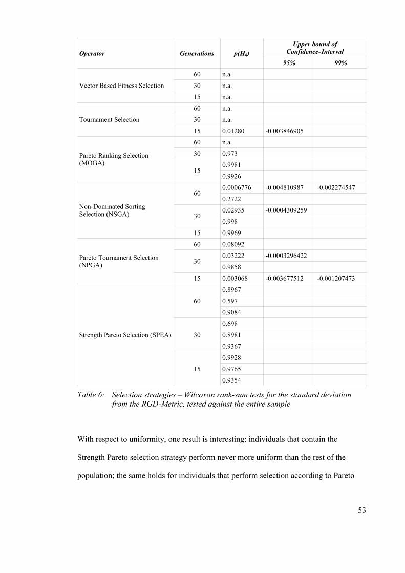
Operator Generations p(H0)
Upper bound of Confidence-Interval
95% 99%
Vector Based Fitness Selection
60 n.a.
30 n.a.
15 n.a.
Tournament Selection
60 n.a.
30 n.a.
15 0.01280 -0.003846905
Pareto Ranking Selection (MOGA)
60 n.a.
30 0.973
150.9981
0.9926
Non-Dominated Sorting Selection (NSGA)
600.0006776 -0.004810987 -0.002274547
0.2722
300.02935 -0.0004309259
0.998
15 0.9969
Pareto Tournament Selection (NPGA)
60 0.08092
300.03222 -0.0003296422
0.9858
15 0.003068 -0.003677512 -0.001207473
Strength Pareto Selection (SPEA)
60
0.8967
0.597
0.9084
30
0.698
0.8981
0.9367
15
0.9928
0.9765
0.9354
Table 6: Selection strategies – Wilcoxon rank-sum tests for the standard deviation from the RGD-Metric, tested against the entire sample
With respect to uniformity, one result is interesting: individuals that contain the
Strength Pareto selection strategy perform never more uniform than the rest of the
population; the same holds for individuals that perform selection according to Pareto
53
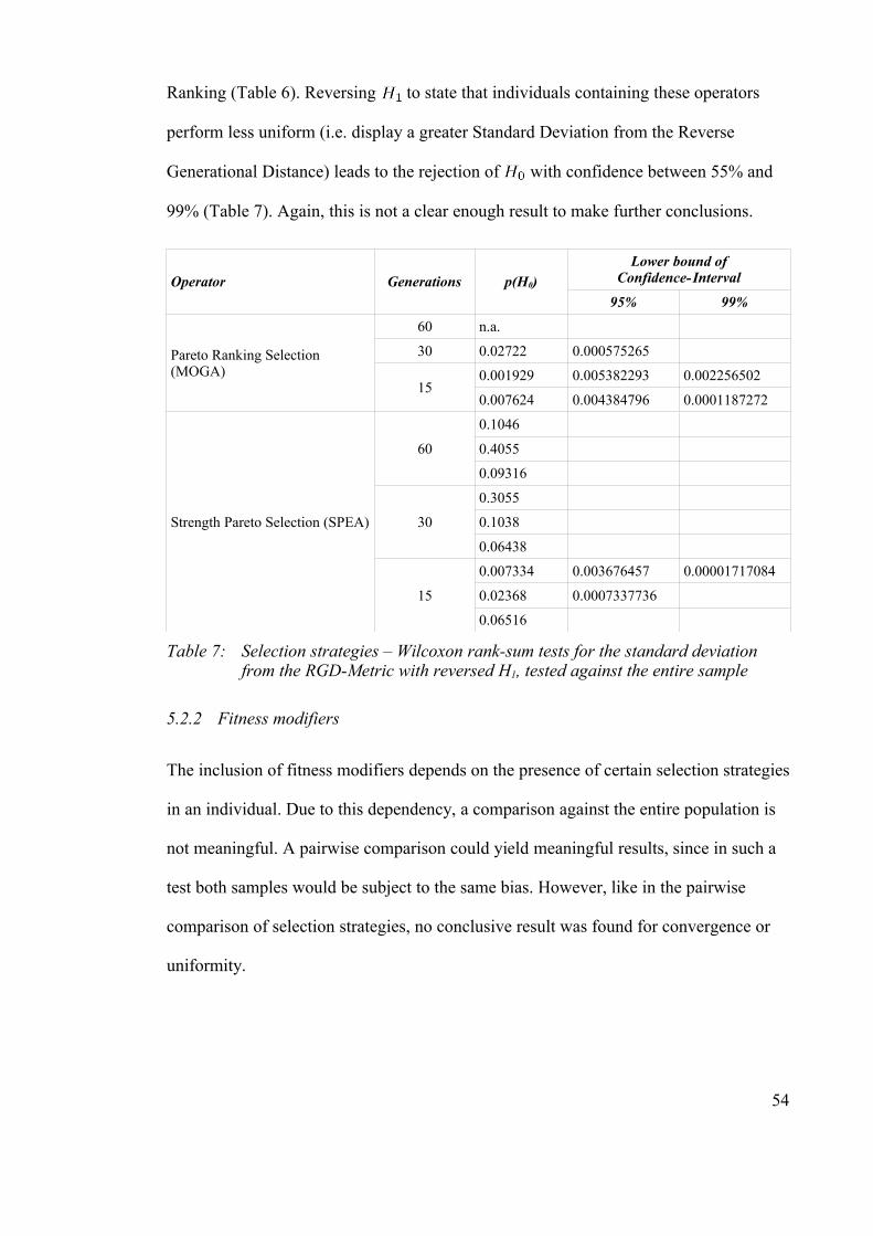
Ranking (Table 6). Reversing to state that individuals containing these operators
perform less uniform (i.e. display a greater Standard Deviation from the Reverse
Generational Distance) leads to the rejection of with confidence between 55% and
99% (Table 7). Again, this is not a clear enough result to make further conclusions.
Operator Generations p(H0)
Lower bound of Confidence-Interval
95% 99%
Pareto Ranking Selection (MOGA)
60 n.a.
30 0.02722 0.000575265
150.001929 0.005382293 0.002256502
0.007624 0.004384796 0.0001187272
Strength Pareto Selection (SPEA)
60
0.1046
0.4055
0.09316
30
0.3055
0.1038
0.06438
15
0.007334 0.003676457 0.00001717084
0.02368 0.0007337736
0.06516
Table 7: Selection strategies – Wilcoxon rank-sum tests for the standard deviation from the RGD-Metric with reversed H1, tested against the entire sample
5.2.2 Fitness modifiers
The inclusion of fitness modifiers depends on the presence of certain selection strategies
in an individual. Due to this dependency, a comparison against the entire population is
not meaningful. A pairwise comparison could yield meaningful results, since in such a
test both samples would be subject to the same bias. However, like in the pairwise
comparison of selection strategies, no conclusive result was found for convergence or
uniformity.
54
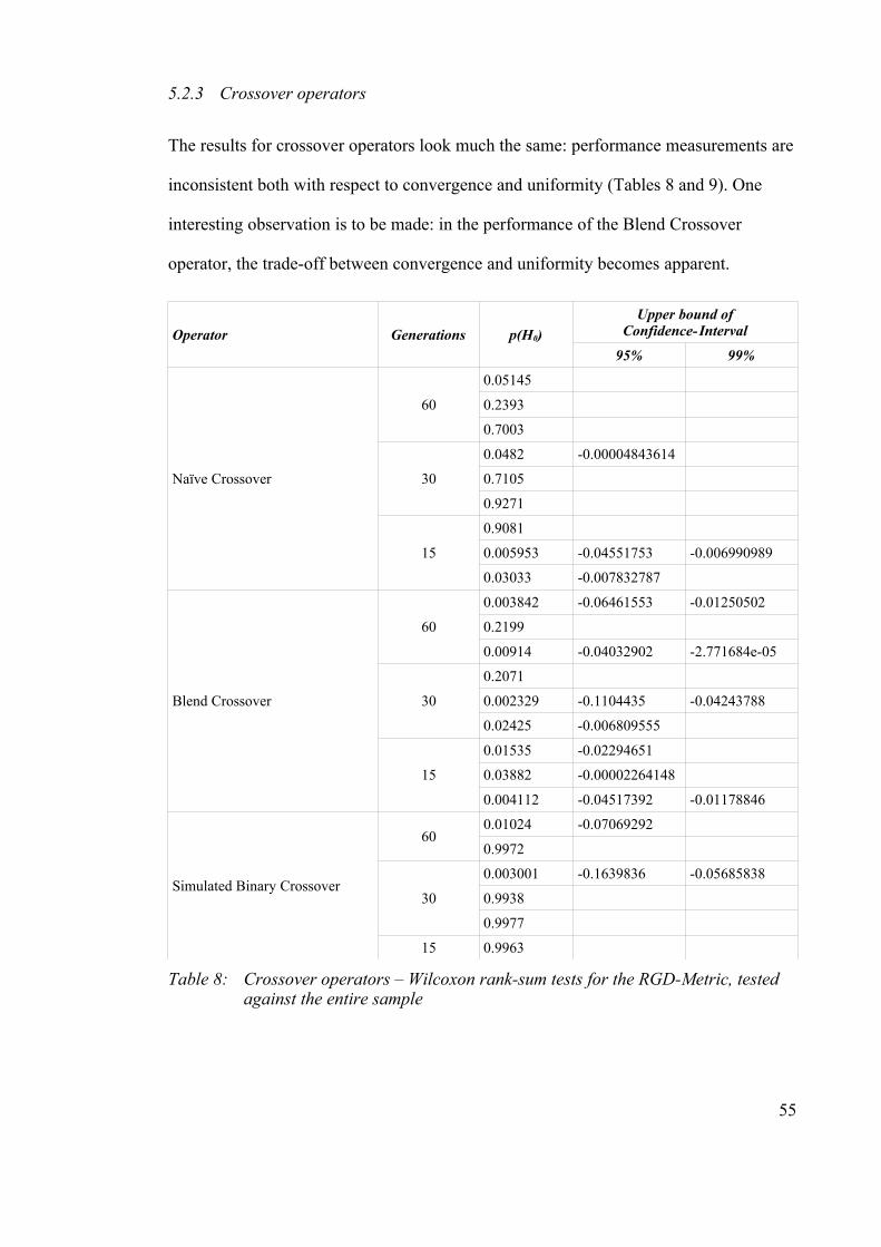
5.2.3 Crossover operators
The results for crossover operators look much the same: performance measurements are
inconsistent both with respect to convergence and uniformity (Tables 8 and 9). One
interesting observation is to be made: in the performance of the Blend Crossover
operator, the trade-off between convergence and uniformity becomes apparent.
Operator Generations p(H0)
Upper bound of Confidence-Interval
95% 99%
Naïve Crossover
60
0.05145
0.2393
0.7003
30
0.0482 -0.00004843614
0.7105
0.9271
15
0.9081
0.005953 -0.04551753 -0.006990989
0.03033 -0.007832787
Blend Crossover
60
0.003842 -0.06461553 -0.01250502
0.2199
0.00914 -0.04032902 -2.771684e-05
30
0.2071
0.002329 -0.1104435 -0.04243788
0.02425 -0.006809555
15
0.01535 -0.02294651
0.03882 -0.00002264148
0.004112 -0.04517392 -0.01178846
Simulated Binary Crossover
600.01024 -0.07069292
0.9972
30
0.003001 -0.1639836 -0.05685838
0.9938
0.9977
15 0.9963
Table 8: Crossover operators – Wilcoxon rank-sum tests for the RGD-Metric, tested against the entire sample
55
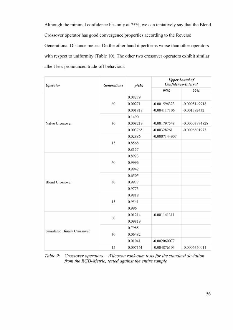
Although the minimal confidence lies only at 75%, we can tentatively say that the Blend
Crossover operator has good convergence properties according to the Reverse
Generational Distance metric. On the other hand it performs worse than other operators
with respect to uniformity (Table 10). The other two crossover operators exhibit similar
albeit less pronounced trade-off behaviour.
Operator Generations p(H0)
Upper bound of Confidence-Interval
95% 99%
Naïve Crossover
60
0.08279
0.00271 -0.001596323 -0.0005149918
0.001818 -0.004117106 -0.001392432
30
0.1490
0.008219 -0.001797548 -0.00003974828
0.003765 -0.00328261 -0.0006801973
15
0.02886 -0.0007144907
0.8568
0.8157
Blend Crossover
60
0.8923
0.9996
0.9942
30
0.6505
0.9977
0.9773
15
0.9818
0.9541
0.996
Simulated Binary Crossover
600.01214 -0.001141311
0.09819
30
0.7985
0.06482
0.01041 -0.002060077
15 0.007161 -0.004876103 -0.0006350011
Table 9: Crossover operators – Wilcoxon rank-sum tests for the standard deviation from the RGD-Metric, tested against the entire sample
56
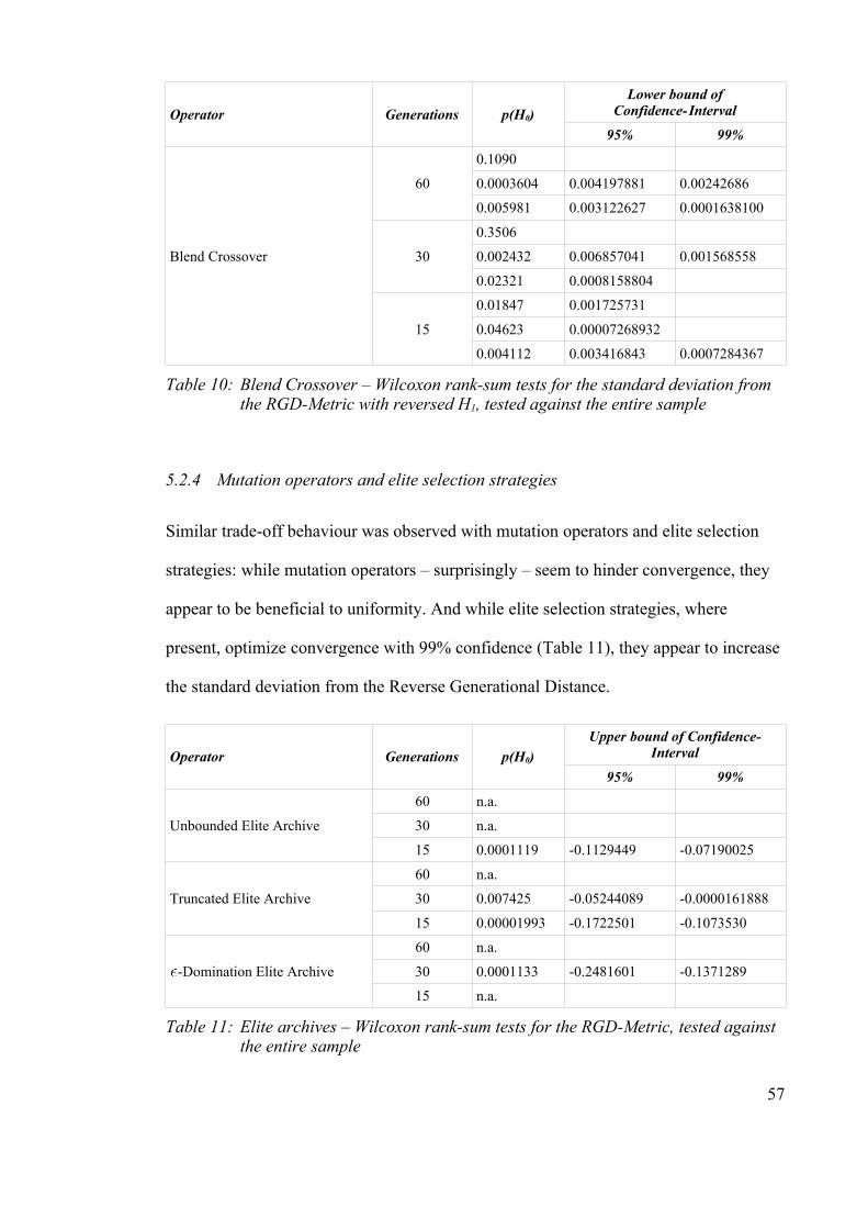
Operator Generations p(H0)
Lower bound of Confidence-Interval
95% 99%
Blend Crossover
60
0.1090
0.0003604 0.004197881 0.00242686
0.005981 0.003122627 0.0001638100
30
0.3506
0.002432 0.006857041 0.001568558
0.02321 0.0008158804
15
0.01847 0.001725731
0.04623 0.00007268932
0.004112 0.003416843 0.0007284367
Table 10: Blend Crossover – Wilcoxon rank-sum tests for the standard deviation from the RGD-Metric with reversed H1, tested against the entire sample
5.2.4 Mutation operators and elite selection strategies
Similar trade-off behaviour was observed with mutation operators and elite selection
strategies: while mutation operators – surprisingly – seem to hinder convergence, they
appear to be beneficial to uniformity. And while elite selection strategies, where
present, optimize convergence with 99% confidence (Table 11), they appear to increase
the standard deviation from the Reverse Generational Distance.
Operator Generations p(H0)
Upper bound of Confidence-Interval
95% 99%
Unbounded Elite Archive
60 n.a.
30 n.a.
15 0.0001119 -0.1129449 -0.07190025
Truncated Elite Archive
60 n.a.
30 0.007425 -0.05244089 -0.0000161888
15 0.00001993 -0.1722501 -0.1073530
-Domination Elite Archive
60 n.a.
30 0.0001133 -0.2481601 -0.1371289
15 n.a.
Table 11: Elite archives – Wilcoxon rank-sum tests for the RGD-Metric, tested against the entire sample
57
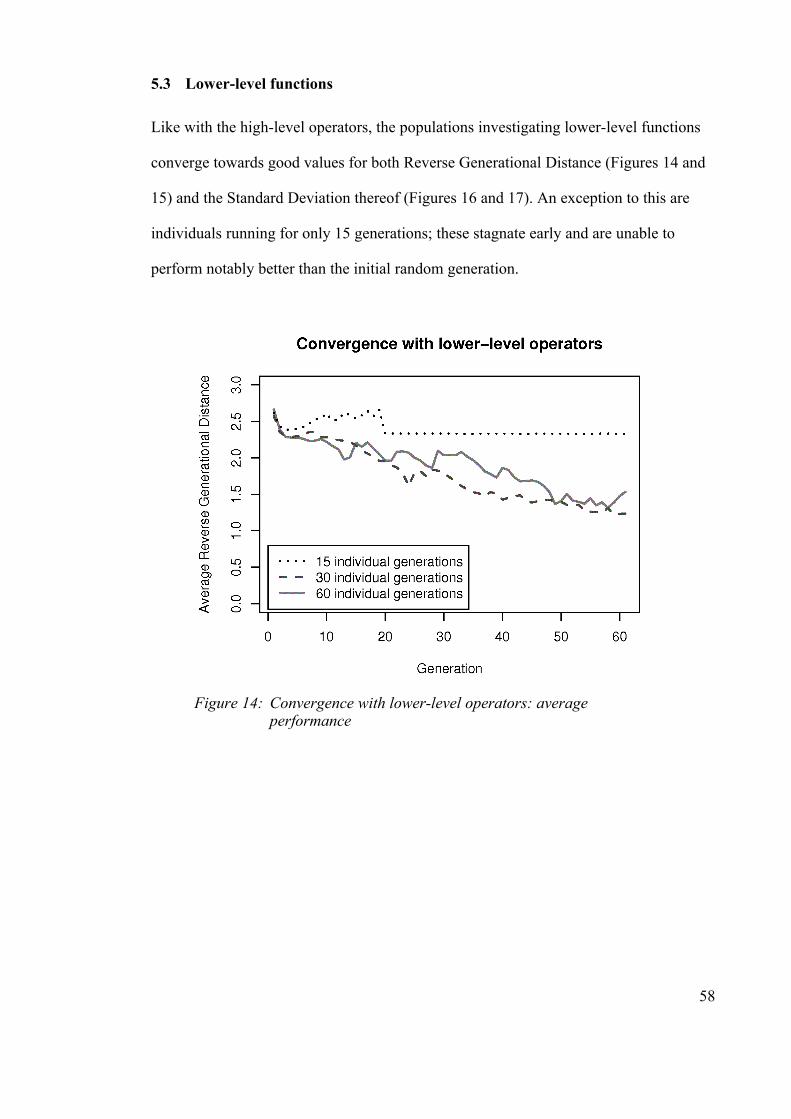
5.3 Lower-level functions
Like with the high-level operators, the populations investigating lower-level functions
converge towards good values for both Reverse Generational Distance (Figures 14 and
15) and the Standard Deviation thereof (Figures 16 and 17). An exception to this are
individuals running for only 15 generations; these stagnate early and are unable to
perform notably better than the initial random generation.
58
Figure 14: Convergence with lower-level operators: average performance
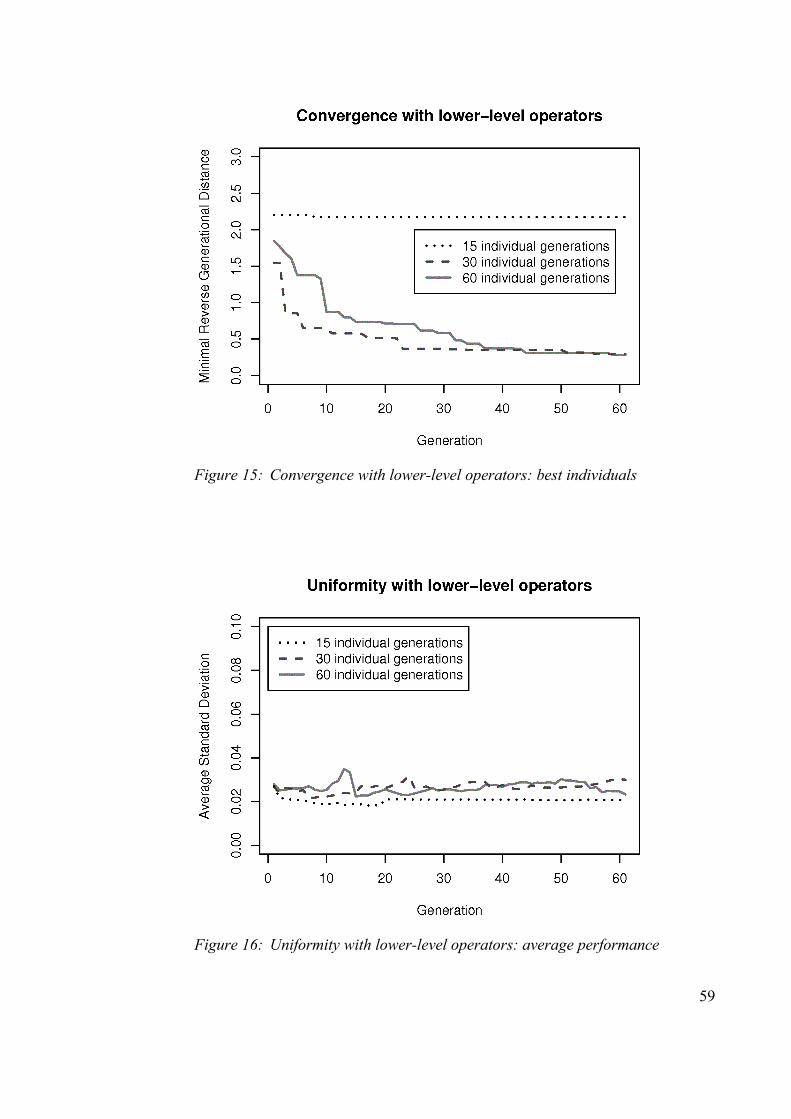
59
Figure 15: Convergence with lower-level operators: best individuals
Figure 16: Uniformity with lower-level operators: average performance
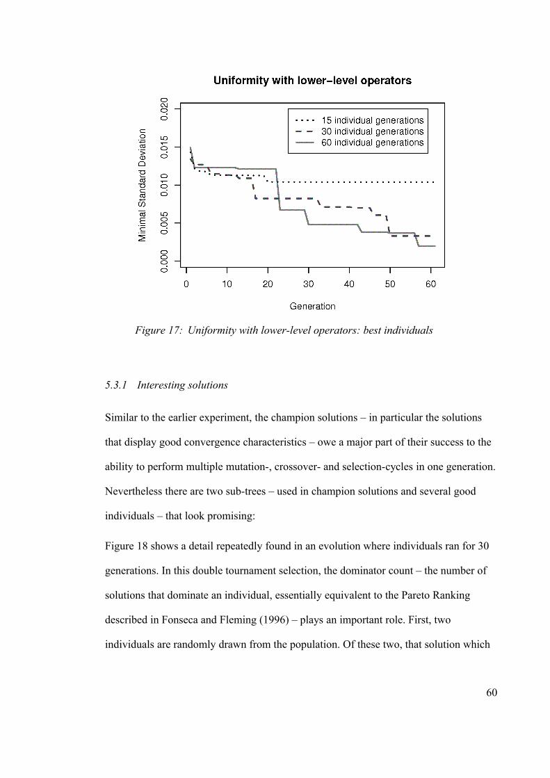
5.3.1 Interesting solutions
Similar to the earlier experiment, the champion solutions – in particular the solutions
that display good convergence characteristics – owe a major part of their success to the
ability to perform multiple mutation-, crossover- and selection-cycles in one generation.
Nevertheless there are two sub-trees – used in champion solutions and several good
individuals – that look promising:
Figure 18 shows a detail repeatedly found in an evolution where individuals ran for 30
generations. In this double tournament selection, the dominator count – the number of
solutions that dominate an individual, essentially equivalent to the Pareto Ranking
described in Fonseca and Fleming (1996) – plays an important role. First, two
individuals are randomly drawn from the population. Of these two, that solution which
60
Figure 17: Uniformity with lower-level operators: best individuals
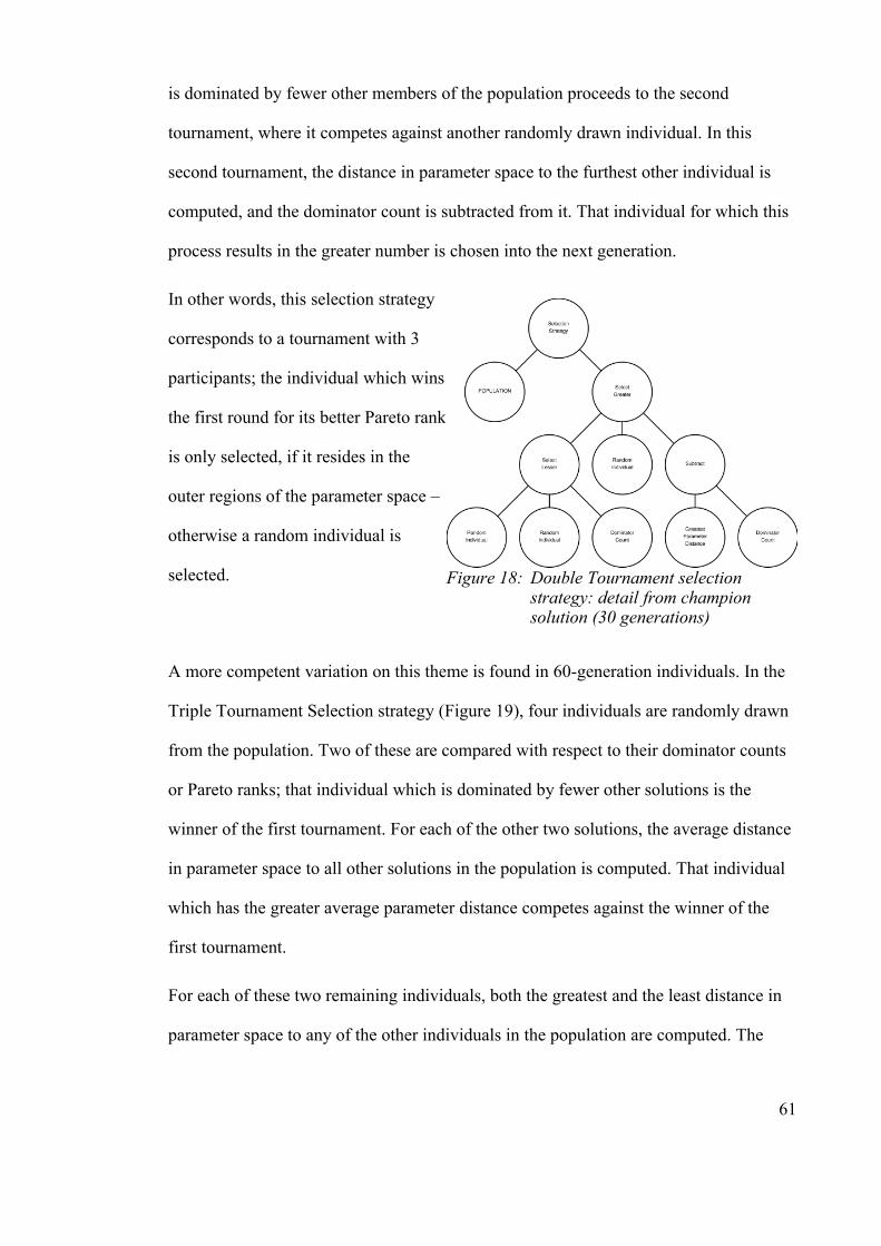
is dominated by fewer other members of the population proceeds to the second
tournament, where it competes against another randomly drawn individual. In this
second tournament, the distance in parameter space to the furthest other individual is
computed, and the dominator count is subtracted from it. That individual for which this
process results in the greater number is chosen into the next generation.
In other words, this selection strategy
corresponds to a tournament with 3
participants; the individual which wins
the first round for its better Pareto rank
is only selected, if it resides in the
outer regions of the parameter space –
otherwise a random individual is
selected.
A more competent variation on this theme is found in 60-generation individuals. In the
Triple Tournament Selection strategy (Figure 19), four individuals are randomly drawn
from the population. Two of these are compared with respect to their dominator counts
or Pareto ranks; that individual which is dominated by fewer other solutions is the
winner of the first tournament. For each of the other two solutions, the average distance
in parameter space to all other solutions in the population is computed. That individual
which has the greater average parameter distance competes against the winner of the
first tournament.
For each of these two remaining individuals, both the greatest and the least distance in
parameter space to any of the other individuals in the population are computed. The
61
Figure 18: Double Tournament selection strategy: detail from champion solution (30 generations)
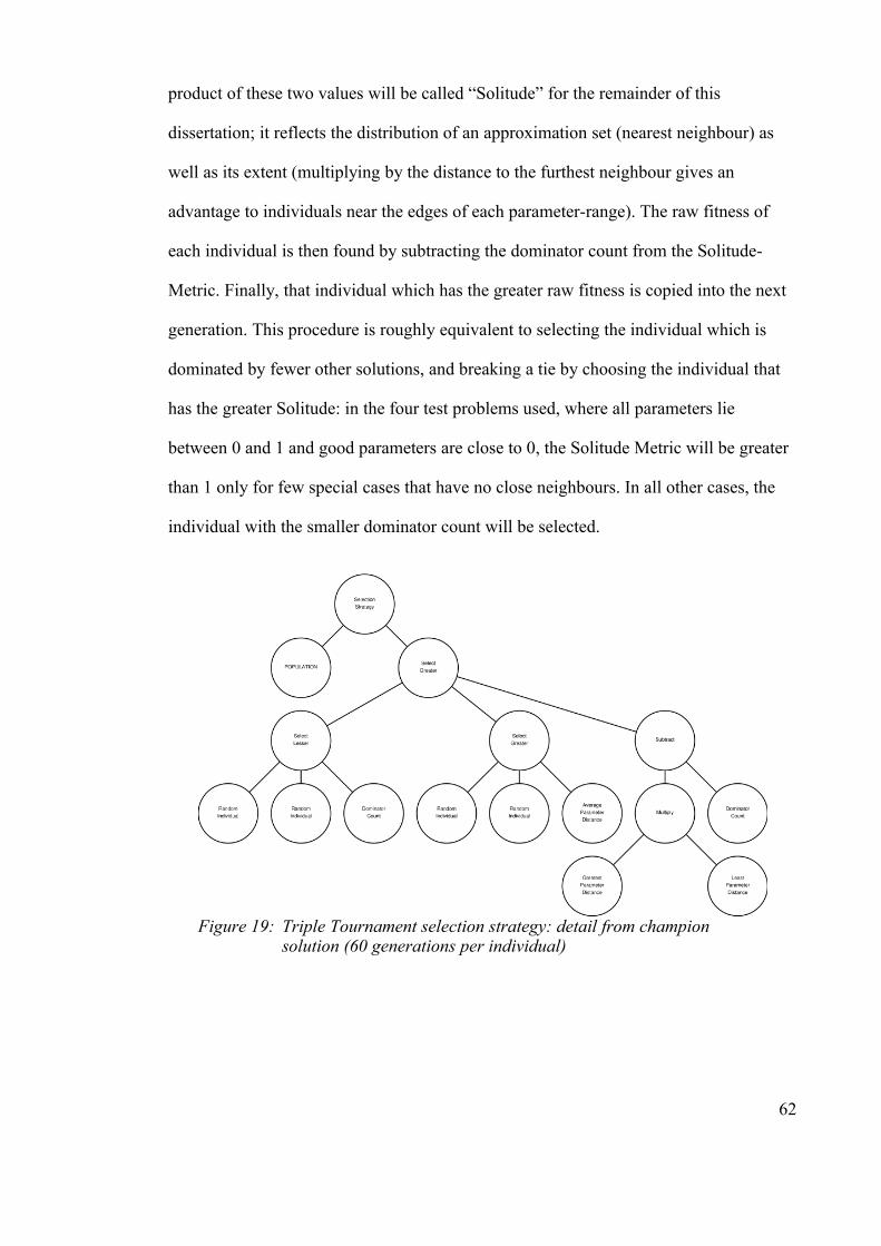
product of these two values will be called “Solitude” for the remainder of this
dissertation; it reflects the distribution of an approximation set (nearest neighbour) as
well as its extent (multiplying by the distance to the furthest neighbour gives an
advantage to individuals near the edges of each parameter-range). The raw fitness of
each individual is then found by subtracting the dominator count from the Solitude-
Metric. Finally, that individual which has the greater raw fitness is copied into the next
generation. This procedure is roughly equivalent to selecting the individual which is
dominated by fewer other solutions, and breaking a tie by choosing the individual that
has the greater Solitude: in the four test problems used, where all parameters lie
between 0 and 1 and good parameters are close to 0, the Solitude Metric will be greater
than 1 only for few special cases that have no close neighbours. In all other cases, the
individual with the smaller dominator count will be selected.
62
Figure 19: Triple Tournament selection strategy: detail from champion solution (60 generations per individual)
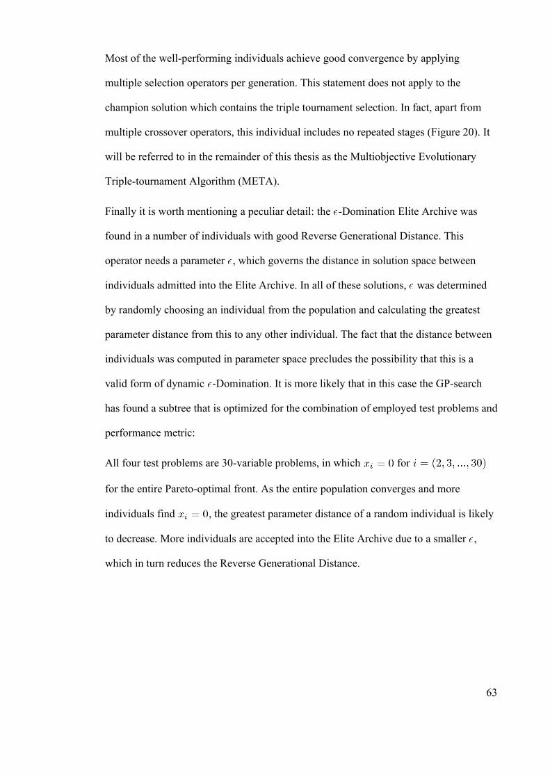
Most of the well-performing individuals achieve good convergence by applying
multiple selection operators per generation. This statement does not apply to the
champion solution which contains the triple tournament selection. In fact, apart from
multiple crossover operators, this individual includes no repeated stages (Figure 20). It
will be referred to in the remainder of this thesis as the Multiobjective Evolutionary
Triple-tournament Algorithm (META).
Finally it is worth mentioning a peculiar detail: the -Domination Elite Archive was
found in a number of individuals with good Reverse Generational Distance. This
operator needs a parameter , which governs the distance in solution space between
individuals admitted into the Elite Archive. In all of these solutions, was determined
by randomly choosing an individual from the population and calculating the greatest
parameter distance from this to any other individual. The fact that the distance between
individuals was computed in parameter space precludes the possibility that this is a
valid form of dynamic -Domination. It is more likely that in this case the GP-search
has found a subtree that is optimized for the combination of employed test problems and
performance metric:
All four test problems are 30-variable problems, in which for
for the entire Pareto-optimal front. As the entire population converges and more
individuals find , the greatest parameter distance of a random individual is likely
to decrease. More individuals are accepted into the Elite Archive due to a smaller ,
which in turn reduces the Reverse Generational Distance.
63
64
Figure 20: Lower-level functions – Champion solution (60 generations per individual)

5.4 Validation
It is apparent from the previous experiments that while it exhibits some difficulties
finding a good combination of high-level operators, a Multi-Objective Genetic
Programming environment can successfully find new selection operators. But how do
these perform in direct comparison to a known good Multi-Objective Algorithm? To
examine their quality, the obtained champion-solution and two of the details extracted
from it were run against NSGA-II:
1. An implementation of the entire champion-solution, including four instances of
crossover and no mutation operator (META).
2. The Triple Tournament Operator used as Selection Operator, with all other
configuration-details identical to NSGA-II (Triple Tournament).
3. A variation of NSGA-II, with the Solitude metric replacing NSGA-II's crowding
distance (Solitude).
These three and NSGA-II were each run over the course of 30, 60 and 100 generations,
with 30 measurements taken per configuration. Appendix A contains comparative box-
plots of these measurements for each configuration.
5.4.1 Results
Neither of the three tested variations is an equivalent replacement for NSGA-II. When
run over the course of 100 generations, NSGA-II consistently found the best
approximation sets. For 60-generation evolutions the Solitude-variant resulted in better
mean values. Finally, the META-variant outperforms all other configurations after 30
generations. This is very probably the effect of forgoing the inclusion of a mutation
operator: good solutions propagate quickly without the deteriorating effects of mutation.
But once the best combinations of all genomes are found – and because no new
65

genomes are introduced – the search stagnates. This also demonstrates the importance
of the choices made for the MOGP System configuration: it seems that the resulting
algorithms have been specialized for being run over few generations.
5.5 Summary
Experiments on the combination of high-level operators yield results consistent with
literature. However, these results are only occasionally statistically significant.
Nevertheless, there is evidence supporting the contribution of selection strategies,
crossover operators and elite archives towards convergence. Of the tested crossover
operators, Blend Crossover leans most aggressively towards convergence, and
contributes least to uniformity. Surprisingly, mutation operators appear to be mainly
responsible for uniform approximation sets.
The search for new selection strategies using lower-level functions yields three
interesting partial trees, two of which are promising candidates. The third is evidence
towards the danger of over-specialization: it is probable that its good performance has
more to do with the nature of the test problems than with Multi-Objective Optimization
in general.
66

Chapter 6 Conclusions
6.1 Project review
This project has investigated the feasibility of nesting Multi-Objective Evolutionary
Algorithms (MOEAs) in Genetic Programming (GP) experiments, with the aim to
search for and find new selection strategies. A number of experiments were conducted,
first exploring the ability of GP to recombine high-level operators into good MOEAs,
later investigating whether new operators could be found from lover-level building
blocks, and finally comparing the obtained results to NSGA-II, one of the best-known
algorithms in the field.
In support of these experiments, a framework for nested evolution was developed both
conceptually and in an implementation based on the Open BEAGLE framework
(Appendix B). While not comprehensive, it offers a broad range of high-level operators
and lower-level functions for inclusion in subsequent investigations. More importantly,
it provides researchers with a structural base that solves the problem of evolving
iterative processes, limited for the special case of evolutionary algorithms. And finally,
it is extensible in so far as building-blocks, test problems and performance metrics can
be replaced with equivalent operators. Limitations include the fact that the generational
structure is constant – as in most GP-Projects, the search space cannot include loop
operators. Overcoming the problems of automatically nested loops and the connected
halting problem are still matters of investigation with researchers examining the
foundations of Genetic Programming. Consequently, the presented framework cannot
model approaches that diverge from classical evolutionary algorithms.
Also prerequisite to the experiments, it was shown that the theoretical limits that govern
unary performance metrics for multi-objective approximation sets can be worked
67
around. The definition of finer-grained comparability – for those cases where two
approximation sets are incomparable according to the dominance relations described by
Hansen and Jaszkiewicz (1998) and Zitzler et al. (2002) – and the arbitrary choice to
favour uniform approximation sets over few champion solutions, together enable two
approximation sets to be compared with a simple process.
The distribution of solutions in the resulting data sets support the initial assumption that
the search for MOEAs is itself a multi-objective problem: all experiments yielded elite
sets with distinct trade-off surfaces that can be observed to converge towards better
solutions as the GP-evolution progresses. However, the recombination of high-level
operators did not yield the expected clear recommendations on which building blocks to
use in which case. In-depth analysis of the obtained data showed several limitations of
the chosen approach: many of the fittest solutions had solved the posed problem by
repeating elements from each functional family (elite-set selection, mutation and
crossover) several times per generation, thus gaining the advantage of additional
generations. This resulted in many ties in the ranking process inherent to the Wilcoxon
rank-sum test, which may explain the fact that few significant differences in the
performance of the employed building-blocks were found. Additionally, a distinct
propensity to specialize was found: the shape of both the search-space and the Pareto-
optimal front defined by the employed test problems influence the generated solutions.
In the four test problems employed in this study, most parameters needed to approach
zero in order for the population to converge towards the Pareto-optimal front. In certain
GP-individuals a specialization for this fact was found. And while it is of course
desirable to find such a specialization in the MOEA-individuals depicting the
approximation set, for the GP-individuals that describe how the approximation set
should be found, a more general proficiency is favoured.
68
It also needs to be noted that the criteria determining the end of an evolution influence
the results: in this study, the number of generations was fixed to a low level, due to the
exceedingly high computational complexity of nested evolutionary algorithms. This has
resulted in a related specialization and in what appears to be a separation of Mutation
and Crossover operators – demonstrated in the validation experiments, where the
absence of a Mutation operator from the Multi-objective Evolutionary Triple-
Tournament Algorithm (META) leads to significantly better results after 30, but also
significantly worse results after 100 generations.
In conclusion we can state that neither of the two hypotheses posed in conjunction with
the research question are unquestionably supported or rejected. While no combination
of high-level building blocks was found which has convergence properties similar to
those of known “good” MOEAs, the insights gained into the process of nested evolution
may enable successful experimental configurations in future research. Similarly, the
search for new selection strategies was more successful than expected: in what is the
most exciting result, two new selection strategies consisting of lower-level functions
were found. One of these is the Triple Tournament Selection operator which includes
the Solitude distance operator, a new and somewhat surprising method of ensuring
diversity.
6.2 Future research
There are several variants of the developed framework that are worth investigating:
since the objective of uniformity is secondary to that of convergence, and since the
standard deviation from the Reverse Generational Distance (RGD) metric was observed
to be several orders of magnitude smaller than the metric itself, it may be worth
combining the two by simple addition. The expected behaviour of such a combined
69

metric would be to select individuals with good convergence properties, while
additionally favouring individuals with slightly worse but significantly more uniform
convergence.
The optimization of program size remains an interesting quandary. In the context of
evolving MOEAs from high-level building blocks, it may be a valid strategy to limit the
program size to the number of identified functional families. In addition to removing
one of the objectives from the multi-objective problem, that approach would also
significantly reduce the search space by limiting the number of possible operator-
combinations.
Many more building-blocks would be possible. Of particular interest are lower-level
functions that provide a form of introspection into the state of the evolution: a
generation counter, the average fitness-improvement from the previous generation, or
other internal information, could be used to influence the relative probability of
mutation and crossover. Can an evolutionary process find such a relation?
Results from this study suggest that – at least for the test problems employed –
crossover is most efficient for short evolutions, whereas mutation is more important in
evolutions over many generations. It seems likely that there are at least two phases in an
evolution, in which a population reacts differently to the operations it is subjected to.
The identification of such phases (for lack of a better example: early, middle and late),
and the role of each genetic operator in these, seem a topic worth exploring, both for the
single- and the multi-objective case. Also of interest is the precise role that the number
of generations per individual plays in the nested evolutionary system.
70
References
Banzhaf, W., Nordin, P., Keller, R. E. and Francone, F.D. (1998) Genetic Programming: An Introduction, San Francisco, Morgan Kaufmann.
Bleuler, S., Brack, M., Thiele, L. and Zitzler, E. (2001) ‘Multiobjective Genetic Programming: Reducing Bloat Using SPEA2’, Proceedings of the 2001 Congress on Evolutionary Computation CEC2001, 536-543.
Bosman, P. and Thierens, D. (2003) ‘The balance between proximity and diversity in multiobjective evolutionary algorithms’, Evolutionary Computation, IEEE Transactions on, 7, 174-188.
Coello Coello, C. A. (2000) ‘An updated survey of GA-based multiobjective optimization techniques’. ACM Comput. Survey, 32, 109-143.
Coello Coello, C. A. (2005) ‘Recent Trends in Evolutionary Multiobjective Optimization’ in Abraham, A., Jain, L. and Goldberg, R. (eds), Evolutionary Multiobjective Optimization, London, Springer.
De Jong, E. D. and Pollack, J.B. (2003) ‘Multi-Objective Methods for Tree Size Control’, Genetic Programming and Evolvable Machines, 4, 211-233.
De Jong, E. D., Watson, R. A. and Pollack, J.B. (2001) ‘Reducing bloat and promoting diversity using multi-objective methods’, Proceedings of the Genetic and Evolutionary Computation Conference, GECCO-2001, 11-18.
De Jong, K. A. (1975) An Analysis of the behavior of a class of Genetic Adaptive Systems, PhD thesis, University of Michigan (Computer and Communication Sciences).
Deb, K. (1999) ‘Multi-Objective Genetic Algorithms: Problem Difficulties and Construction of Test Problems’, Evolutionary Computation, 7, 205-230.
Deb, K., Agrawal, S., Pratab Amrit and Meyarivan, T. (2000) A Fast Elitist Non-Dominated Sorting Genetic Algorithm for Multi-Objective Optimization: NSGA-II, (KanGAL Report No. 200001), Indian Institute of Technology Kanpur.
Deb, K. (2001) Multi-Objective Optimization Using Evolutionary Algorithms, Chichester, Wiley.
Deb, K., Mohan, M. and Mishra Shikhar (2005) ‘Evalutating the e-Domination Based Multi-Objective Evolutinary Algorithm for a Quick Computation of Pareto-Optimal Solutions’, Evolutionary Computation, 4, 501-525.
Deb, K., Thiele, L., Laumanns, M. and Zitzler, E. (2002) ‘Scalable Multi-Objective Optimization Test Problems’, Congress on Evolutionary Computation (CEC'2002), 1, 825-830.
Ekárt, A. and Németh, S.Z. (2001) ‘Selection Based on the Pareto Nondomination Criterion for Controlling Code Growth in Genetic Programming’, Genetic Programming and Evolvable Machines, 2, 61-73.
71

Farhang-Mehr, A. and Azarm, S. (2002) ‘Diversity Assessment of Pareto Optimal Solution Sets: An Entropy Approach’, Proceedings of the 2002 Congress on Evolutionary Computation, CEC '02, 723-728.
Farhang Mehr, A. and Azarm, S. (2002) ‘Entropy-Based Multi-Objective Genetic Algorithm for Design Optimization’, Journal of Structural and Multidisciplinary Optimization, 24, 351-361.
Fonseca, C. M. and Fleming, P.J. (1993) ‘Genetic Algorithms for Multiobjective Optimization: Formulation, Discussion and Generalization’, Genetic Algorithms: Proceedings of the Fifth International Conference, 416-423.
Fonseca, C. M. and Fleming, P.J. (1996) ‘On the Performance Assessment and Comparison of Stochastic Multiobjective Optimizers’, PPSN IV: Proceedings of the 4th International Conference on Parallel Problem Solving from Nature, 584-593.
Friedberg, R. (1958) ‘A learning machine: Part i’, IBM Journal of Research and Development, 2, 2-13.
Gagné, Ch. and Parizeau, M. (2006) ‘Genericity in Evolutionary Computation Software Tools: Principles and Case-Study’, Journal on Artificial Intelligence Tools, 15, 173-194.
Goldberg, D. E. (1989) Genetic Algorithms in Search, Optimization and Machine Learning, Addison Wesley.
Greene, W. A. (2005) ‘Schema Disruption in Tree-Structured Chromosomes’, Proceedings of the 2005 conference on Genetic and evolutionary computation, 1401 - 1408.
Gruau, F. and Whitley, D. (1993) ‘Adding learning to the cellular development of neural networks: Evolution and the Baldwin effect’, Evolutionary Computation, 1, 213-233.
Hanne, T. (1999) ‘On the convergence of multiobjective evolutionary algorithms’, European Journal of Operational Research, 117, 553-564.
Hansen, M. P. and Jaszkiewicz, A. (1998) Evaluating the quality of approximations to the non-dominated set, (IMM-REP-1998-7). Institute of Technical Modeling, Technical University of Denmark.
Hernández-Díaz, A. G., Santana-Quintero, L. V., Coello Coello, C., Caballero, R. and Molina, J. (2006) ‘A New Proposal for Multi-Objective Optimization using Differential Evolution and Rough Sets Theory’, Proceedings of the 8th annual conference on Genetic and evolutionary computation (GECCO'06), 675 - 682.
Holland, J. H. (1975) quoted in Goldberg, D. E. (1989) Genetic Algorithms, Addison Wesley.
Hollstien, R. B. (1970) quoted in Goldberg, D. E. (1989) Genetic Algorithms, Addison Wesley.
72
Horn, J. and Nafpliotis, N. (1993) Multiobjective Optimization using the Niched Pareto Genetic Algorithm (IlliGAl Report 93005), Department of General Engineering, University of Illinois at Urbana-Champaign.
Hu, X. and Eberhart, R. (2002) ‘Multiobjective Optimization using Dynamic Neighborhood Particle Swarm Optimization’, IEEE Proceedings, World Congress on Computational Intelligence (CEC'02), 1677-1681.
Hwang, C. and Masud, A.S.M. (1979) quoted in Deb, K. (2001) Multi-Objective Optimization using Evolutionary Algorithms, Chichester, Wiley.
Ishibuchi, H. and Murata, T. (1996) ‘Multi-objective genetic local search algorithm’, Proceedings of IEEE International Conference on Evolutionary Computation, 119-124.
Knowles, J. and Corne, D. (2002) ‘On metrics for comparing non-dominated sets’, Congress on Evolutionary Computation (CEC 2002), 666-673.
Koza, J. R. (1990) Genetic Programming: A Paradigm for Genetically Breeding Populations of Computer Programs to Solve Problems (STANCS901314), Stanford University Computer Science Dept., Stanford CA.
Koza, J. R. (1994) Genetic Programming II, Automatic Discovery of Reusable Programs, MIT-Press.
Koza, J. R. (1995) ‘Evolving the Architecture of a Multi-Part Program in Genetic Programming Using Architecture-Altering Operations’, Evolutionary Programming IV Proceedings of the Fourth Annual Conference on Evolutionary Programming, 695-717.
Koza, J. R., Bennett, F. H. and Stiffelman, O. (1999) ‘Genetic Programming as a Darwinian Invention Machine’, Proceedings of the Second European Workshop on Genetic Programming, 93-108.
Langdon, W. B. and Poli, R. (2002) Foundations of Genetic Programming, Berlin, Springer.
Laumanns, M., Thiele, L., Deb, K. and Zitzler, E. (2002) ‘Combining Convergence and Diversity in Evolutionary Multi-Objective Optimization’, Evolutionary Computation, 10, 263-282.
Laumanns, M., Thiele, L., Deb, K. and Zitzler, E. (2001) On the Convergence and Diversity-Preservation Properties of Multi-Objective Evolutionary Algorithms (TIK-Report No. 108), Swiss Federal Institute of Technology (ETH), Zurich.
Pardoe, D., Ryoo, M. and Miikkulainen, R. (2005) ‘Evolving neural network ensembles for control problems’, Proceedings of the 2005 conference on Genetic and evolutionary computation, 1379-1384.
Parks, G. T. and Miller, I. (1998) ‘Selective Breeding in a Multiobjective Genetic Algorithm’, Proceedings of the 5th International Conference on Parallel Problem Solving from Nature, 250-259, London, Springer.
73

R Development Core Team (2006) R: a language and environment for statistical computing, R Foundation for Statistical Computing, Vienna, Austria.
Rinne, H. (2003) Taschenbuch der Statistik, Frankfurt am Main, Harri Deutsch.
Rodriguez-Vazquez, K., Fonseca, C. M. and Fleming, P.J. (1997) ‘Multiobjective Genetic Programming: A Nonlinear System Identification Application’, Late Breaking Papers at the 1997 Genetic Programming Conference, 207-212.
Rudolph, G. (1996) ‘Convergence of evolutionary Algorithms in general Search spaces’, Evolutionary Computation, 1996., Proceedings of IEEE International Conference on, 50-54.
Rudolph, G. (1998) ‘Evolutionary Search for Minimal Elements in Partially Ordered Finite Sets’, Proceedings of the Seventh Annual Conference on Evolutionary Programming (EP VII), 1447, 345-353.
Rudolph, G. (2001) ‘Evolutionary Search under Partially Ordered Fitness Sets’, Proceedings of the International NAISO Congress on Information Science Innovations (ISI 2001), 8, 818-822.
Rudolph, G. (2001) ‘Some Theoretical Properties of Evolutionary Algorithms under Partially Ordered Fitness Values’, Proceedings of the Evolutionary Algorithms Workshop (EAW-2001), 9-22.
Schaffer, J. D. (1984) quoted in Deb, K. (2001) Multi-Objective Optimization using Evolutionary Algorithms, Chichester, Wiley.
Schott, J. R. (1995) quoted in Deb, K. (2001) Multi-Objective Optimization using Evolutionary Algorithms, Chichester, Wiley.
Srinivas, N. and Deb, K. (1994) ‘Multiobjective Optimization Using Nondominated Sorting in Genetic Algorithms’, Evolutionary Computation, 2, 221-248.
Turing, A. M. (1950) ‘Computing Machinery and Intelligence’, Mind, LIX, 433-460.
Van Veldhuizen, D. A. (1999) Multiobjective Evolutionary Algorithms: Classifications, Analyses and New Innovations, PhD thesis, Graduate School of Engineering, Air Force Institute of Technology, Wright-Patterson AFB, OH.
Van Veldhuizen, D. A. and Lamont, G.B. (1998) ‘Evolutionary Computation and Convergence to a Pareto Front’, Late Breaking Papers at the Genetic Programming 1998 Conference, 221-228.
Xin Yao (1999) ‘Evolving artificial neural networks’, Proceedings of the IEEE, 87, 1423-1447.
Zitzler, E. (1999) Evolutionary Algorithms for Multiobjective Optimization: Methods and Applications, PhD thesis, Swiss Federal Institute of Technology, Zurich.
Zitzler, E. and Thiele L. (1998) An Evolutionary Algorithm for Multiobjective Optimization: The Strength Pareto Approach (TIK-Report 43), Swiss Federal Institute of Technology (ETH), Zurich.
74

Zitzler, E. and Thiele, L. (1998) ‘Multiobjective Optimization Using Evolutionary Algorithms - A Comparative Case Study’, Parallel Problem Solving from Nature, V (PPSN-V), 292-301.
Zitzler, E., Deb, K. and Thiele, L. (2000) ‘Comparison of Multiobjective Evolutionary Algorithms: Empirical Results’, Evol. Comput, 8, 173-195.
Zitzler, E., Laumanns, M. and Thiele, L. (2001) SPEA2: Improving the Strength Pareto Evolutionary Algorithm for Multiobjective Optimization (TIK-Report 103), Swiss Federal Institute of Technology (ETH), Zurich.
Zitzler, E., Thiele, L., Laumanns, M., Fonseca, C. M. and Grunert da Fonseca, V. (2002) Performance assessment of multiobjective optimizers: an analysis and review (TIK-Report 139), Swiss Federal Institute of Technology (ETH), Zurich.
75

Index
Aggregating functions.......................................................................................................5
approximation set..................................................................................................3, 12, 28
Attainment Surface Metric..............................................................................................13
code-bloat........................................................................................................................10
convergence.......................................................................................................................6
Convergence-comparable................................................................................................30
crossover operator........................................................................................................5, 26
decision-maker...................................................................................................................3
distribution.........................................................................................................................6
Distribution-comparable..................................................................................................30
diversity.............................................................................................................................6
dominance relations.........................................................................................................28
elite archive......................................................................................................................21
elitism................................................................................................................................6
Entropy Metric.................................................................................................................15
Error Ratio.......................................................................................................................14
extent.................................................................................................................................6
Generational Distance metric..........................................................................................13
generations.........................................................................................................................4
Genetic Programming....................................................................................................1, 7
global optimum..................................................................................................................3
Hypervolume Metric........................................................................................................14
76

incomparable...................................................................................................................29
introns..............................................................................................................................11
local optimum....................................................................................................................3
Maximum Pareto Front Error..........................................................................................14
Maximum Spread Metric.................................................................................................15
Multi-Objective Genetic Algorithm................................................................................20
Multi-Objective Optimization...........................................................................................3
Multiobjective Evolutionary Triple-tournament Algorithm............................................63
mutation operator...............................................................................................................4
shrink...........................................................................................................................26standard.......................................................................................................................26sub-tree swap..............................................................................................................26swap............................................................................................................................26
Niched Pareto Genetic Algorithm...................................................................................20
Non-dominated Sorting Genetic Algorithm....................................................................21
NSGA-II....................................................................................................................22, 26
Open BEAGLE Framework............................................................................................26
outperformance relation...................................................................................................16
Pareto-based approaches....................................................................................................6
Pareto-nondomination.......................................................................................................4
Pareto-optimal front...........................................................................................................4
Pareto-optimal set..............................................................................................................4
Pareto-optimal set ...........................................................................................................12
Pareto-optimal solution......................................................................................................3
population..........................................................................................................................4
Population-based...............................................................................................................5
77
Reverse Generational Distance..................................................................................16, 31
Set Coverage Metric........................................................................................................14
Solitude............................................................................................................................62
Spacing Metric.................................................................................................................13
Sparsity Measure.............................................................................................................16
Spread Metric..................................................................................................................15
Strength Pareto Evolutionary Algorithm.........................................................................21
test problems....................................................................................................................17
trade-off.............................................................................................................................3
Triple Tournament Selection...........................................................................................61
Vector Evaluated Genetic Algorithm..............................................................................19
Wilcoxon rank-sum test...................................................................................................33
78
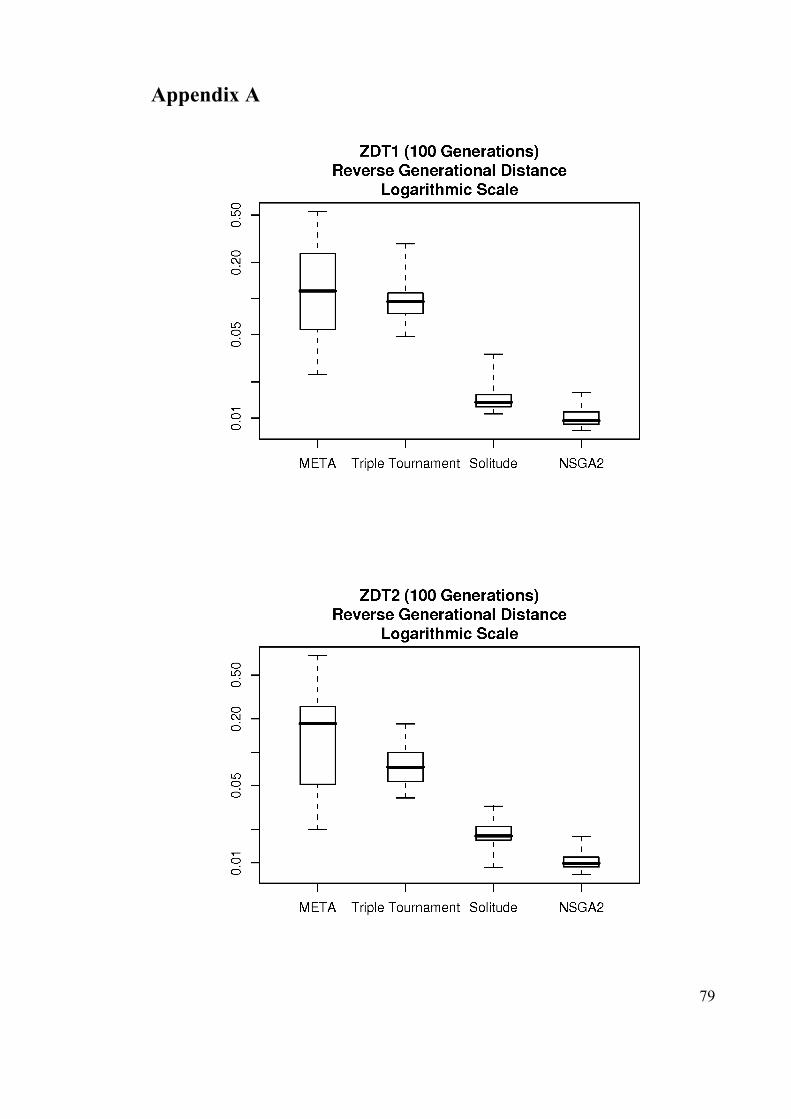
Appendix A
79
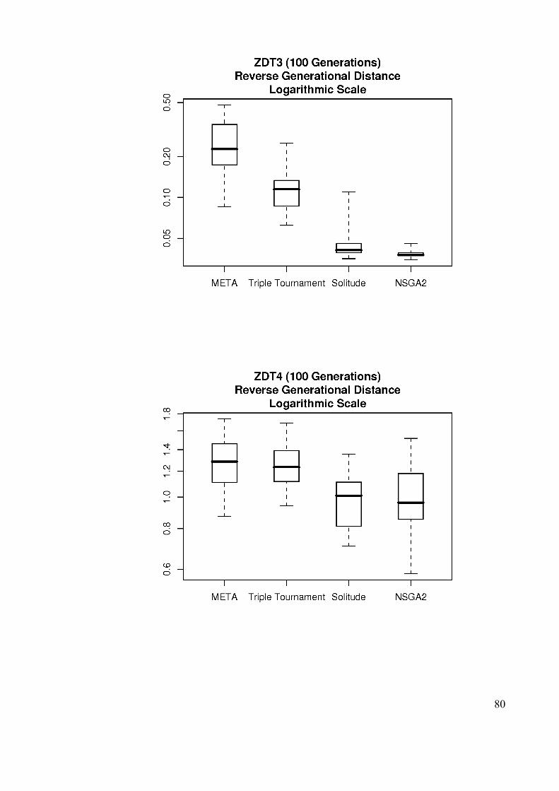
80

81
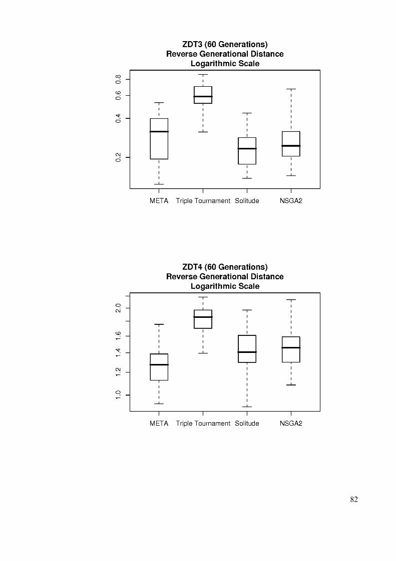
82
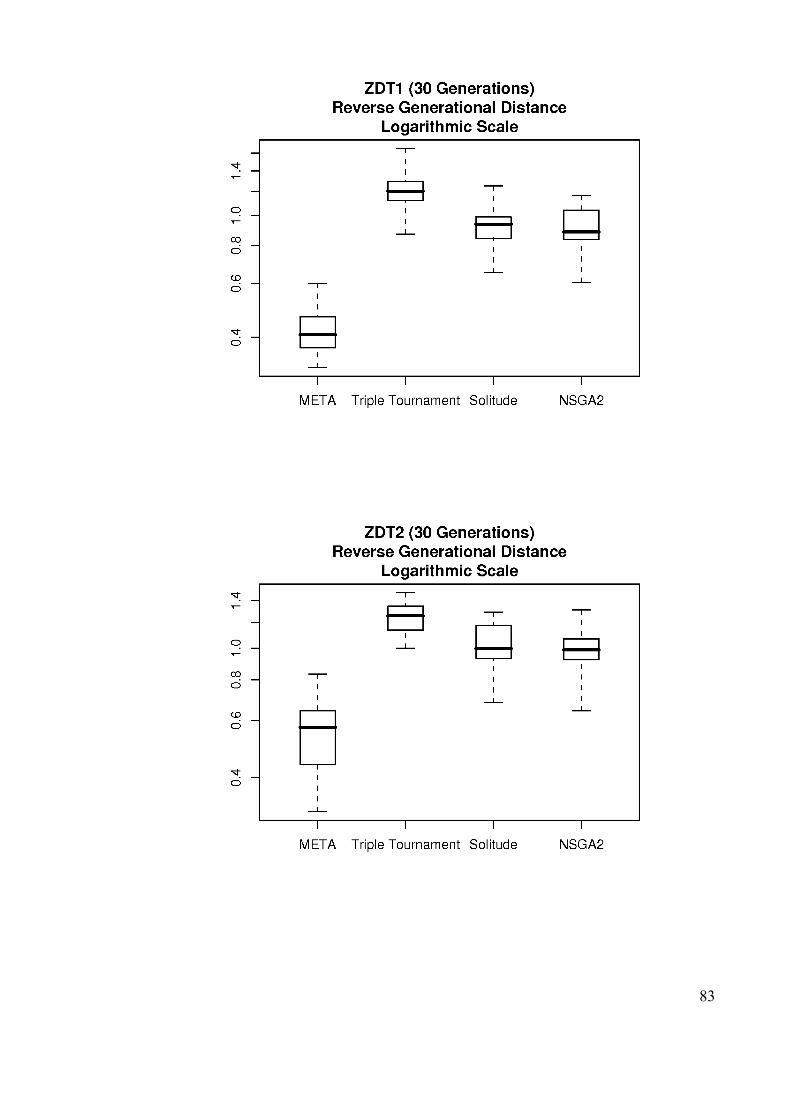
83
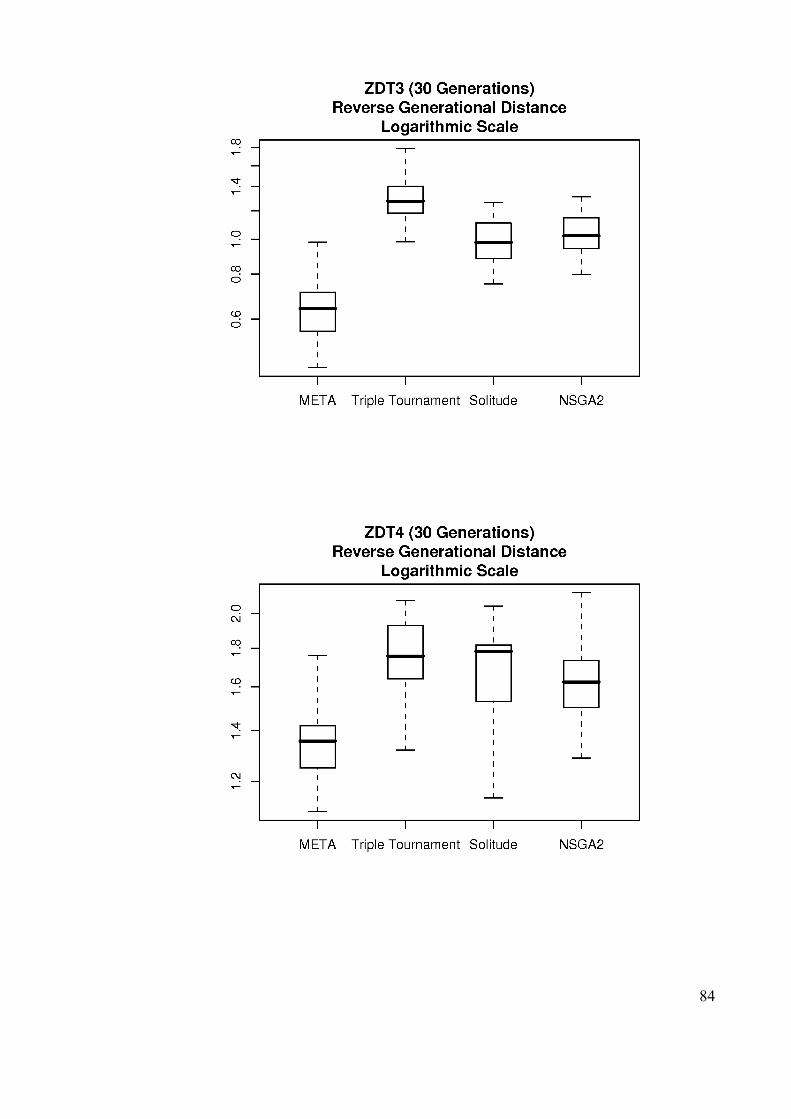
84

Appendix B
85