Evolving yield curves in the real-world measures: a …quantlabs.net/academy/download/free_quant_instituitional_books... · 30 Riccardo Rebonato, Sukhdeep Mahal, Mark Joshi, Lars-Dierk

In this paper we show how to evolve a yield curve over time horizons of the order of years using a simple but effective semiparametric method. The pro-posed technique preserves in the limit all the eigenvalues and eigenvectors of the observed changes in yields. It also recovers in a satisfactory way several important statistical features (unconditional variance, serial autocorrelation, distribution of curvatures, eigenvectors) of the real-world data. A simple finan-cial explanation can be provided for the methodology. The possible financial applications are discussed.

1 Introduction and motivation

1.1 The setting

The literature on models to evolve the yield curve is vast, and entire books have been devoted to the topic. The evolution from the early short rate-based models to the modern pricing approach has been highlighted, for instance, in Morton (1996), Brigo and Mercurio (2001), Rebonato (2002), etc. These models, however, prescribe how a yield curve should evolve if a trader wanted to price a replicable interest rate derivative and avoid arbitrage. At the root of this pricing approach is the (Girsanov) transformation between the real-world (objective) measure and the pricing measure. The constraints on this transformation are very weak, and they amount to the principle of absolute continuity and to the equivalence of the real-world and pricing measures. Even when markets can be assumed to be com-plete, this pricing measure is in general not unique, depending as it does on the

29

Evolving yield curves in the real-world measures: a semi-parametric approach

Riccardo RebonatoRoyal Bank of Scotland, 135 Bishopsgate, London EC2M 3UR

Sukhdeep MahalRoyal Bank of Scotland, 135 Bishopsgate, London EC2M 3UR

Mark JoshiRoyal Bank of Scotland, 135 Bishopsgate, London EC2M 3UR

Lars-Dierk Buchholzd-fine GmbH, Opernplatz 2, 60313, Frankfurt am Main, Germany

Ken NyholmRisk Management Division, European Central Bank, Kaiserstraße 29, Frankfurt am Main,

Germany

Volume 7/Number 3, Spring 2005 URL: www.thejournalofrisk.com

Riccardo Rebonato, Sukhdeep Mahal, Mark Joshi, Lars-Dierk Buchholz, and Ken Nyholm30

numeraire chosen for present-valuing of future payoffs. Depending on the chosen numeraire, the resulting measure is described by different names (risk-neutral measure, forward measure, terminal measure, etc).

The non-uniqueness of the pricing measure is even more clear when perfect replication is not possible. In this case there exist in fact an infinity of pricing mea-sures consistent with absence of arbitrage. To each of these pricing measures and numeraires there corresponds a different set of drifts to be applied to the relevant financial quantities (eg, forward rates) to avoid arbitrage and therefore different evolutions of the universe of interest rate-based assets.

This multiplicity of measures causes no concern for relative pricing purposes but creates an ambiguity for applications that require the real-world evolution of the yield curve. This is because in many applications what it required is a simulation of the real-world evolution, as opposed to one of the many possible arbitrage-free evolutions, of the yield curve. This is the problem addressed in this paper. What these applications are is reviewed in the next subsection.

1.2 Possible applicationsThe applications alluded to above are numerous and important. Some examples are the following.

1.2.1 Evaluation of potential future exposure (PFE) for counterparty credit risk assessmentThis case is typically associated with off-balance sheet transactions (such as swaps) which require zero or minimal outlay of cash up-front, but which expose the counterparty to a potential future credit exposure according to whether the deal will be in the money at the time of a possible future default. In order to evaluate the PFE the relevant yield curve will have to be evolved, typically using a Monte Carlo procedure, and the conditional exposure in the various states of the world computed.

1.2.2 Assessment of the hedging performance of interest rate option modelsJudging the quality of a model from the plausibility of its assumptions is notori-ously a dangerous task. The strongest test to which a new interest rate pricing model or calibration methodology can be put is a hedging “beauty context” against a rival approach. Clearly, the result will strongly depend on the assumed real-world dynamics of the yield curve. Not surprisingly, if, as customary, the real-world yield curve is assumed to be shocked by a few eigenvalues obtained from the orthogonalization of the covariance matrix, the hedging strategy suggested by a simple diffusive pricing model with deterministic volatilities will produce a good replication of the payoff of a plain-vanilla option. This is more likely to be due, however, to the very simplified nature of the yield curve evolution than to any intrinsic virtues of the modeling approach.

1.2.3 Assessment of different investment strategies in interest rate-sensitive investment portfolios (Asset/liability management)

Investment portfolios are typically not managed (nor is their performance com-

URL: www.thejournalofrisk.com Journal of Risk

Evolving yield curves in the real-world measures: a semi-parametric approach 31

monly assessed) on the basis of a daily mark-to-market. It is more common for their performance to be evaluated with reference to the net interest income (NII) that they generate. Since it is not difficult to “engineer” a favorable NII over a short period of time, it is essential that the evaluation of the relative NII performance of competing interest rate-based portfolios should be assessed over a suitably long time horizon.

1.2.4 Economic capital calculationsTypically with these techniques the marginal contribution of a new investment or a business activity to a total loss profile is estimated. The desirability of the proposed new investment is assessed on the basis of the trade-off between return and some measure of portfolio risk. These applications can be used to allocate scarce capital, or to evaluate the performance of business lines, and require the construction of a profit-and-loss profile over horizons of at least one year. In these applications the evolution of yield curves plays an important role because the loss profile is affected by interest rates not only directly (eg, via traded interest rate-sensitive instruments) but also indirectly via the behavioralization of, say, depositors’ behavior or mortgage pre-payment patterns.

1.3 Common requirements of these applicationsAll these applications have some important features in common.

❑ The evolution of the yield curve must be carried out over a potentially very long time horizon (many years).

❑ The resulting yield curves must be accurately representative of the population of the future yield curves, since misleading results can easily be obtained if an over-stylized model evolution is chosen.

❑ Typically, contingent on a state of the world being reached in the future, the evaluation of the fair future conditional value of trading instruments will have to be carried out: for PFE calculations, the future value of, say, a swap will have to be calculated; for the assessment of hedging strategies option positions will have to be re-valued, re-hedged and rebalanced; for NII calculations a re-investment strategy will call for the estimate of the future “par coupon” of the conditional securities. All these applications will require switching from the real-world to one of the future pricing measures. Therefore the real-world evolution of the yield curve complements but does not substitute the sampling of the risk-adjusted measure.

The most important difference between these and related applications on the one hand and the more common value-at-risk-based (VAR-based) calculations on the other is the length of the time horizon. For trading-book applications the time interval over which the change in risk factors gives rise to profit and loss variations ranges from one to a few days. While it is difficult to make totally general and process-independent statements, it is in general safe to say that, over these short time periods, the stochastic term will dominate the deterministic component. See, eg, Jorion (1997). In particular, if the underlying real-world processes were simple



diffusions, the drift term would scale as ∆t, but the innovation component as √∆ t. To give an order-of-magnitude estimate, for ∆t =1 day, the drift term would have to be approximately 20 times as large as the diffusive coefficient to make a com-parable impact on the total price move.

One can no longer rely on this dominance of the stochastic term, however, when time horizons are as long as many years. We shall show below that a careful treatment of the deterministic term becomes necessary in these situations, and is actually at the heart of the approach we suggest.1

1.4 Features of the proposed approach and plan of the paper

We have highlighted in general terms the common desiderata for a real-world yield curve simulator to be of use for the applications above. In summary, these are the length of evolution horizon; the requirement of good statistical representativeness of the synthetic yield curves; and the ability to generate a realistic future state of the world, contingent upon which a conditional risk-neutral valuation can be car-ried out.2 We propose in this paper a simple methodology to produce evolutions of yield curves in the real-world measure that satisfy these requirements. More specifically, the approach enjoys the following features:

❑ asymptotically, it reproduces exactly the eigenvalues and the eigenvectors of the real-world one-day changes;

❑ asymptotically, it reproduces exactly the unconditional variance, skewness, kurtosis, etc, of the one-day changes in all the reference rates used to describe the yield curve (the benchmark yields);

❑ it recovers approximately the distribution of yield curve curvatures;❑ it recovers approximately the unconditional variance for many-day changes in

the benchmark yields;❑ it recovers approximately the serial autocorrelation function for one-and many-

day changes in the benchmark yields;❑ it is very simple to implement;❑ it does not make strong statistical assumptions about the generating joint pro-

cess, and requires very few parameters: for n benchmark yields, approximately 2n parameters will be required for the evolution of the whole yield curve over several years;

❑ the most important parameters introduced (the “spring constants”) are finan-cially motivated.

In arriving at this model, we do not make assumptions about the generating stochastic process. In particular, we do not assume that the innovations are either identically or independently distributed. This is important because we document

1 Since our approach is not based on the specification of a joint process, the “drift term” appears in our case as a set of “springs”. These are in turn financially motivated.2 This last requirement rules out approaches that only produce unconditional joint distri-butions of the variables that described the yield curve, no matter how accurate these might be.



(and manage to reproduce with our procedure) a strong positive serial autocorrela-tion for n-day returns.

The model is very parsimonious: the only free parameters are the spring con-stants (equal in number to the number of independent yields minus 2), the window length, the out-of-window jump frequency, two reversion levels and two reversion speeds.

In order to specify the algorithm we introduce a simple financial mechanism that attempts to mimic the behavior of pseudo-arbitrageurs active along the yield curve. We believe this financial mechanism to be plausible and convincing, but we do not set out to test this hypothesis directly. A careful study would require too long a detour and would justify a paper in itself. We therefore present our financial story as a conjecture. It is important to point out, however, that the algorithmic results would remain valid even if the financial mechanism were not true. If the validity of the financial mechanism is accepted, we show that the observed data can be explained as the result of a “tug-of-war” between two competing contributing factors: a positive serial correlation present at all maturities, plus a superimposed quasi-arbitrage activity that introduces negative serial autocorrelation. In our “financial story” we argue that this activity should be more pronounced at the long end of the maturity spectrum. Taken together, the two features (maturity-dependent activity of the pseudo-arbitrageurs and positive serial autocorrelation) can explain both the smoothly-changing behavior of the serial autocorrelation as a function of maturity and the behavior of the n-day unconditional variances observed in the real data.

Our methodology will be presented in stages, starting from a totally non-parametric approach. We have chosen this style of presentation, which is admittedly slightly more cumbersome, because it allows a clear understanding of the origin of the shortcomings of the various “partial solutions”, and why the approach we have chosen is necessary. For instance, the presentation of the totally-non-parametric algorithm (Section 4.1) both shows the inadequacy of PCA-based approaches and points to the importance of the maturity dependence of the serial correlation. This in turn motivates the financial conjecture alluded to above.

The paper is organized as follows. Section 2 discusses the links of our work with the existing literature. Section 3 describes the data. A naïve first approach, and its shortcomings, are described in Section 4. Section 5 shows how its problems can be overcome by adding a simple model of the behavior of pseudo-arbitrageurs and presents the main results of the paper. A discussion is presented in Section 6 of the advantages and disadvantages of using absolute or percentage changes. An overall discussion and suggestions for future work are to be found in Section 7.

2 Links with the existing literature

Beside the approach investigated in this paper, there exist at least two other types of model that can be used to evolve the yield curve over long horizons, namely term-structure models designed for pricing purposes and models that attempt to provide a statistical description of the evolution of rates in the objective measure.



2.1 Pricing models

Starting from the pricing models, two further subclasses should be distinguished: pricing models that make use of a joint specification of the risk premia and of the real-world dynamics (“fundamental” models), and pricing models that directly describe the evolution of the yield curve in the risk-neutral measure (and that I will therefore refer to as “reduced-form” models). The distinction is important. The focus of both these classes of model is on pricing (of bonds or derivatives) and therefore the results ultimately inhabit the pricing measure. However, the fun-damental approach starts from a stylized specification of the real-world dynamics of the yield curve, to which a description of the investors’ risk aversion (market price of risk) is superimposed. Therefore, the fundamental pricing models, once stripped of their utility-function superstructure, could in principle be used to describe the real-world evolution of the yield curve.3 Even if their stated goal has never been modeling realism, they have nevertheless attempted to capture in a syn-thetic and parsimonious way the salient features of the term structure dynamics. Therefore they afford valuable conceptual insight and could be of some practical use for long-only portfolios; but they cannot – nor have they been designed to – capture more subtle features of the evolution of rates.4

Fundamental models for the evolution of the yield curve have been proposed (in approximate chronological order), for instance, by Vasicek (1977), Cox Ingersoll and Ross (1985), Brennan and Schwartz (1982), and Longstaff and Schwartz (1992). The Brennan and Schwartz model deserves, in this context, a special mention. Their original formulation, based on the evolution of the short rate and of the consol yield, was dynamically unstable (see Hogan, 1993). Variations on the Brennan and Schwartz theme can, however, be introduced that obviate this problem by making the spread between the long and the short rate mean-reverting. This choice generates a co-integrated model, with complex long-term relation-ships between different parts of the yield curve. Indeed, the modeling choice in Equation (5) of this paper similarly introduces a co-integrated feature of sorts to the joint processes describing the yield curve.

The specification of reduced-form pricing models is quite different, in that the description is directly carried out in the risk-neutral measure. Examples of this modeling approach are, for instance, Ho and Lee (1986), Hull and White (1990), and Heath, Jarrow and Morton (1989). The relatively recent appearance of “smiles” in the implied volatility curve has suggested that jumps (see, eg, Glasserman and Kou, 2000), stochastic volatility (see, eg, Joshi and Rebonato, 2003), or a CEV-type behavior (see, eg, Andersen and Andreasen, 1999) might also be important.

3 Note however that, depending on the strategy employed for its calibration, the same model can be fundamental or reduced-form. See Hughston and Brody (2000) and Hughston (2000) for an excellent unified treatment of the two approaches.4 Neither the Vasicek, nor the CIR nor the Longstaff and Schwartz models can reproduce exactly today’s yield curve, let alone its evolution.



All these models work directly in the pricing measure. Most of their parameters (eg, reversion speeds, jump frequencies, etc) implicitly embed, after calibration to market prices, a component linked to risk aversion and therefore contain drift terms different from what is observable in the objective measure. These drift terms, as is perfectly appropriate for the relative-pricing application for which they have been devised, drive a wedge between the real-world and the risk-adjusted evolution of the yield curve. As mentioned above, over long horizons, the evolu-tions produced by these approaches become totally dominated by the no-arbitrage drift term and bear virtually no resemblance to the real-world evolution. For these reasons, the reduced-form models are therefore inappropriate for the applications discussed in Section 1.2 of this paper.

As for the fundamental models, which could, in principle, be used for evolving the yield curve in the objective measure if divorced of their specification of the investors’ risk aversion, they were never designed for this purpose. Their strengths are to be found in the insight that they afford in the essential drivers of the yield curve dynamics. Much as, say, the Ising mode in physics, they are elegant and intriguingly simple models, but they do not attempt to display great realism. The Vasicek and the CIR models, for instance, cannot even recover an arbitrary exogenous yield curve, and their specifications of the market price of risk (either constant or proportional to the square root of the short rate) are blatantly chosen to allow analytical tractability. Therefore, the fundamental pricing models are also inappropriate for the applications discussed in Section 1.2 of this paper.

2.2 Statistical models

Moving away from pricing applications, a copious body of research has focused on the real-world evolution of the term structure. One of the best known is the study by Chan, Karolyi, Longstaff and Sanders (1992), who carry out a parametric estimation of some of the drivers of the process (in particular, the volatility). A related but different (non-parametric) approach is followed by Stanton (1997), who focuses on the US$ three-month Treasury Bill rate and obtains a similar estimate as Chan et al for the volatility but discovers strong evidence for non-linearity in the drift. Stanton also estimates from the data the market price of risk. The approach by Stanton inspired the work by Prigent, Renault and Scaillet (2000), who study the dynamics of the 10-year maturity yield of corporate bonds.

Another important modeling strand rests on a vector autoregressive (real-world) specification of changes in the short rate and spreads to longer rates. See, for example, Campbell and Shiller (1987), Hall, Anderson and Granger (1992), Kugler (1990), and Lanne (2000). In this modeling framework rates are assumed to be co-integrated since changes in the short rate and the spreads to longer rates are treated as stationary variables. Naturally, nominal rates cannot be pure I(1) processes because they are bounded at zero and cannot go to infinity. The reason for modeling rates within a co-integrated system of variables is that the persistence pattern is better approximated in this way, as opposed to a situation where the rates are modeled as stationary variables.



Applications of this modeling framework to interest rates has often been used to test the expectation hypothesis, even though it is equally applicable to the pre-diction of rates. In the literature, applications are frequently limited to bivariate systems, ie, to the evolution of two rates only. While this can be adequate for a qualitative description of the evolution of the yield curve, for the application men-tioned in the introductory section this is too restrictive.

Another class of statistical models focuses on regime-switches in the parame-ters characterizing the mean, the mean-reversion speed and the volatility of the short rate process and generally allows for the presence of two states. See, eg, Ang and Bekaert (2002), Dai, Singleton and Yang (2003), Bansal and Zhou (2002), Driffill, Kenc and Sola (2003), Bansal, Tauchen and Zhou (2003), and Evans (2003).

There are several studies of specific portions of the yield curve, especially of the very short end (the “short rate’). Ait-Sahalia (1996), for instance, argues that the short rate should be close to a random walk in the middle of its historical range (approximately between 4% and 17%), but strongly mean-reverting outside this range. Hamilton (1989), Garcia and Perron (1996), Gray (1996), Ang and Bekaert (1998), Naik and Lee (1997) and Bansal and Zhou (2002), among others, argue that a switch behavior, with a reversion level and reversion speed for each regime, should be more appropriate.

This evolution of the yield curve could be carried out in a statistical framework using principal component analysis. There have been a very large number of studies in this direction, many of which have been recently reviewed in Martellini and Priaulet (2001). Whatever the true process driving the yield curve, the eigen-vectors and eigenvalues always convey interesting summary information about the underlying dynamics. Unfortunately, while informative from a descriptive point of view, these investigations are only valid for the purpose of reproducing the dynamics of the yield curve if the underlying joint process were indeed a dif-fusion, with iid increments. We find in our investigation strong evidence to reject both these hypotheses.

Finally, it has been shown by Rebonato and Cooper (1995) that any model that uses a small number of driving factors brings about the intrinsic inability to recover an exogenous correlation matrix among yields.

Summarizing, none of these approaches tackles the problem of the joint evo-lution, first, of a whole yield curve; second, over long time horizons; third, with possibly many independent drivers; fourth, without imposing independence of the increments; and fifth, while recovering exactly any observed correlation among the rates. Achieving this is the goal of this work. Whether having all these features is truly indispensable clearly depends on the application.

It goes without saying that our approach is not without its shortcomings. Its very lack of a strong structure does not lend itself to a ready intuitive understanding of the essential drivers of the yield curve dynamics. Therefore, it may not be suit-able if a qualitative, parsimonious description of the yield curve is sought. Also, its “algorithmic” specification makes it difficult to predict a priori whether other



important features of the yield curves not built into the evolution procedure are correctly captured. Brute-force simulation and analysis of the results is therefore often the only possible investigative route. At this writing, for instance, studies are being carried out in parallel to explore two distinct features of our model: first, its ability to recover the observed distribution of drawdowns; and second, it ability to recover the features predicted by regime-switching models, such as the BNH model mentioned above.

Having said this, our model is not totally structure-free. This is not just because we will have to introduce some constraints on the deterministic innovation part of the implicit (and unknown) process, but also because we have to choose whether the observed changes should be interpreted as proportional or absolute (or otherwise). The results we present below are obtained using the proportional assumption (that is guaranteed to ensure positivity to all the future rates). We revisit this topic, however, in the second-to-last last section of the paper.

3 The empirical data

3.1 Description

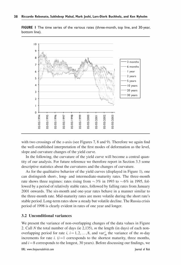
We have data for US$ LIBOR curves from September 29, 1993, to December 4, 2001 (2,135 days). The three-, six- and 12-month rates are deposit rates. After the 12-month maturity, rates are par swap rates. The yield curve is assumed to be described by eight points (benchmark maturities), located at three and six months, and one, two, five, 10, 20 and 30 years. The associated yields are given for three months, six months, one year, two years, five years, 10 years 20 years and 30 years. The whole data set therefore consists of 2,135 × 8 = 17,080 points. The time behavior of each rate is presented in Figure 1. The data set was carefully checked for outliers, and, wherever dubious points were encountered, corroboration was sought from independent sources. We chose to work with par rates rather than, say, with forward rates, because the former can be obtained from observed prices in a model-independent way, while the specific technique used to distill forward rates could easily produce spurious statistical results. As for the treatment of week-ends and holidays, the sampling window method described later on (which typically covers five to six weeks) ensures that most of week-end effects, if any, are correctly captured, with the only possible exception of the joining point of two different sampling windows.

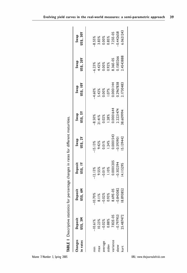
We present in Table 1 the mean, standard deviation, skew and kurtosis of the changes in the rates. We observe that the volatility as a function of the maturity has a maximum around the one-year rate. We also note that the mean of the changes is very close to zero.

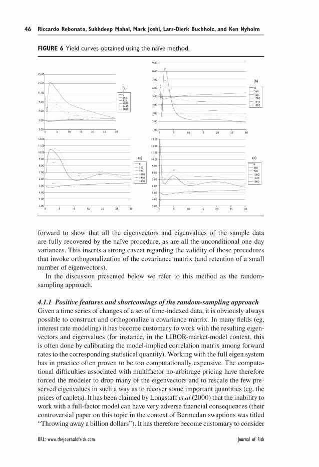
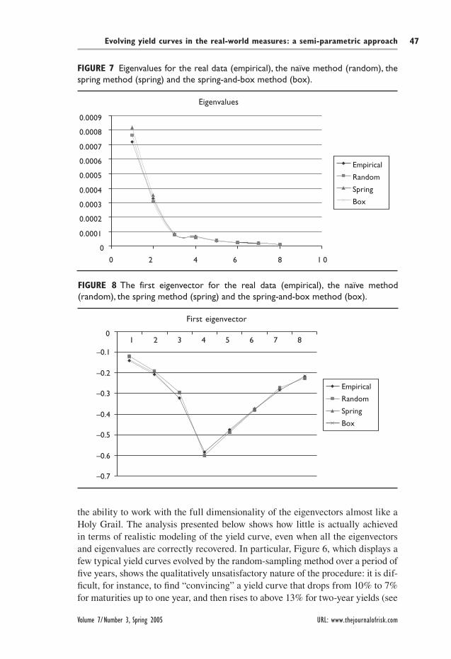
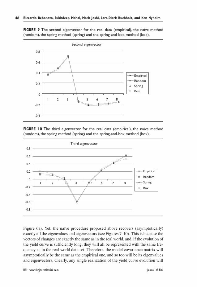
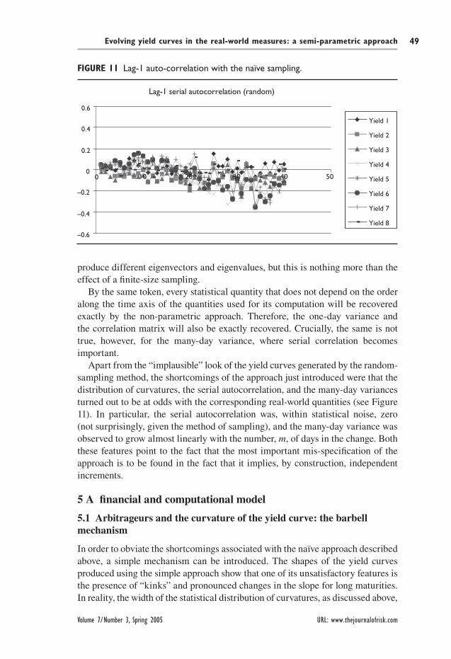
We performed a principal component analysis of the historic data, obtained by orthogonalizing the matrix of the percentage changes in rates. We observed that the first component explains more than 90% of the variance. We also see that the first eigenvector has loadings of the same sign for all the yields, the second eigenvector displays one sign change, and the third eigenvector has a “V” shape,



with two crossings of the x-axis (see Figures 7, 8 and 9). Therefore we again find the well-established interpretation of the first modes of deformation as the level, slope and curvature changes of the yield curve.

In the following, the curvature of the yield curve will become a central quan-tity of our analysis. For future reference we therefore report in Section 3.3 some descriptive statistics about the curvatures and the changes of curvature.

As for the qualitative behavior of the yield curves (displayed in Figure 1), one can distinguish short-, long- and intermediate-maturity rates. The three-month rate shows three regimes: rates rising from ∼ 3% in 1993 to ∼ 6% in 1995, fol-lowed by a period of relatively stable rates, followed by falling rates from January 2001 onwards. The six-month and one-year rates behave in a manner similar to the three-month rate. Mid-maturity rates are more volatile during the short rate’s stable period. Long-term rates show a steady but volatile decline. The Russia crisis period of 1998 is clearly evident in rates of one year and longer.

3.2 Unconditional variances

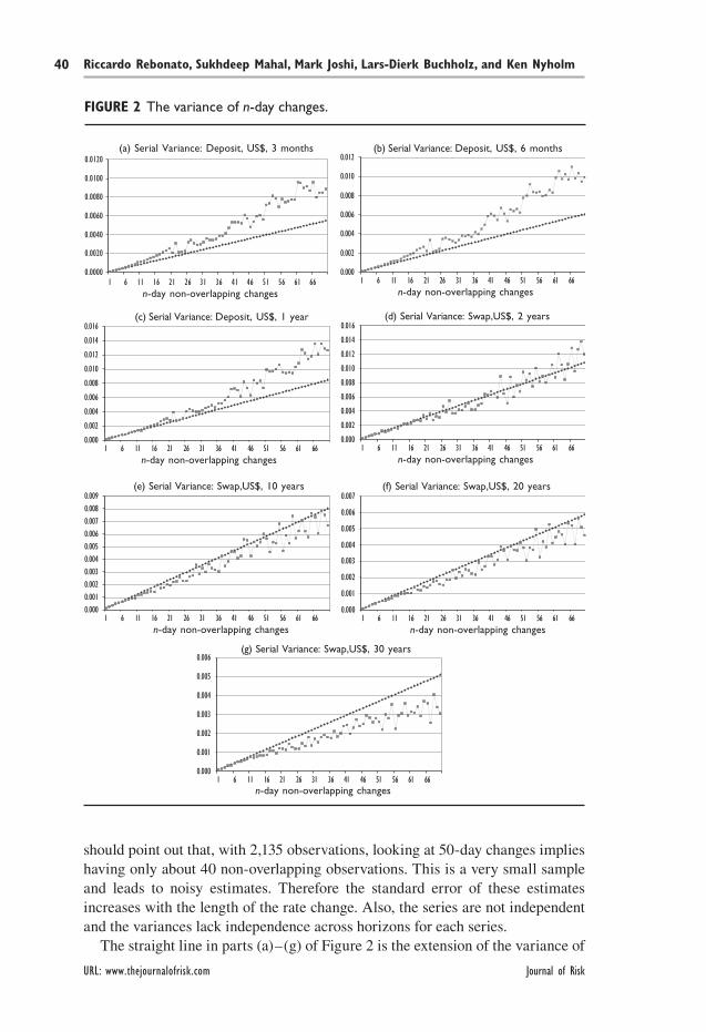
We present the variance of non-overlapping changes of the data values in Figure 2. Call N the total number of days (ie 2,135), m the length (in days) of each non-overlapping period for rate i, i = 1, 2, … , 8, and var i

m the variance of the m-day increments for rate i. (i =1 corresponds to the shortest maturity, three months, and i =8 corresponds to the longest, 30 years). Before discussing our findings, we

FIGURE 1 The time series of the various rates (three-month, top line, and 30-year, bottom line).

0

1

2

3

4

5

6

7

8

9

10

05/0

5/19

94

05/0

5/19

95

05/0

5/19

96

05/0

5/19

97

05/0

5/19

98

05/0

5/19

99

05/0

5/20

00

05/0

5/20

01

05/0

5/20

02

05/0

5/20

03

3 months

6 months

1 year

2 years

5 years

10 years

20 years

30 years



TABL

E 1

Des

crip

tive

stat

istic

s fo

r pe

rcen

tage

cha

nges

in r

ates

for

diffe

rent

mat

uriti

es.

Chan

ges

Dep

osit

Dep

osit

Dep

osit

Swap

Sw

ap

Swap

Sw

ap

Swap

in r

ates

US$

, 3M

US$

, 6M

US$

, 1Y

US$

, 2Y

US$

, 5Y

US$

, 10

Y US$

, 20

Y US$

, 30

Y

min

–1

0.61

%

–10.

70%

–1

2.13

%

–15.

13%

–8

.50%

–

4.60

%

–6.

23%

–8

.55%

max

10

.23%

8.

11%

9.

55%

9.

42%

21

.41%

5.

42%

4.

42%

3.

83%

aver

age

–0.

02%

–

0.02

%

–0.

01%

0.

01%

0.

02%

0.

00%

0.

00%

0.

00%

stde

v 0.

88%

0.

93%

1.

10%

1.

24%

1.

28%

1.

07%

0.

92%

0.

85%

vari

ance

7.

82E-

05

8.69

E-05

0.

0001

205

0.00

0154

3 0.

0001

644

0.00

0114

4 8.

36E-

05

7.25

E-05

skew

–

0.79

7953

–

0.84

3082

–

0.30

2394

–

0.59

3901

2.

2221

474

0.29

6783

8 0.

1583

266

–0.

4426

58ku

rt

25.4

8747

2 18

.893

852

14.1

1529

5 15

.139

442

38.6

0999

4 2.

1730

483

2.45

4388

8 6.

0621

243



should point out that, with 2,135 observations, looking at 50-day changes implies having only about 40 non-overlapping observations. This is a very small sample and leads to noisy estimates. Therefore the standard error of these estimates increases with the length of the rate change. Also, the series are not independent and the variances lack independence across horizons for each series.

The straight line in parts (a)–(g) of Figure 2 is the extension of the variance of

FIGURE 2 The variance of n-day changes.

(a) Serial Variance: Deposit, US$, 3 months

0.0000

0.0020

0.0040

0.0060

0.0080

0.0100

0.0120

1 6 11 16 21 26 31 36 41 46 51 56 61 66n-day non-overlapping changes

(b) Serial Variance: Deposit, US$, 6 months

0.000

0.002

0.004

0.006

0.008

0.010

0.012


(c) Serial Variance: Deposit, US$, 1 year

0.000

0.002

0.004

0.006

0.008

0.010

0.012

0.014

0.016


(d) Serial Variance: Swap,US$, 2 years

0.000

0.002

0.004

0.006

0.008

0.010

0.012

0.014

0.016


(e) Serial Variance: Swap,US$, 10 years

0.0000.0010.0020.0030.0040.0050.0060.0070.0080.009


(f) Serial Variance: Swap,US$, 20 years

0.000

0.001

0.002

0.003

0.004

0.005

0.006

0.007


(g) Serial Variance: Swap,US$, 30 years

0.000

0.001

0.002

0.003

0.004

0.005

0.006




the one-day changes, var i1. So, the quantity

var im = m var i

1 (1)

would be the variance of the m-day changes that would be observed if the incre-ments were iid.5 We clearly see a deviation from linearity in the behavior of the true one-day variance. As the length of the non-overlapping periods increases, rates of short maturities show higher variance than would be obtained if the increments were iid. We remark at this point that a less-then-linear increase in the m-day variance could be compatible with positive autocorrelation.

When we move to longer maturities, as the length of the non-overlapping periods increases, these longer-maturity rates display a variance that increases less than linearly with the length of the non-overlapping period. We remark at this stage that this observation could be compatible with mean reversion.

As mentioned above, as the number of days, m, in each overlapping period increases we have fewer and fewer observations, and our estimates of the m-day variances become noisier and noisier. Even with these caveats, and with the observations above regarding the lack of independence of the variances, the effect appears to be consistent and to display a smooth behavior across maturities.

3.3 Distribution of curvatures

An important statistic for the analysis we present in Section 4 is the distribution of yield curve curvatures. We define the curvature, ξi, at point τi = (Ti+1 − T1−1) ⁄ 2, i = 2, 3, … , 7 between three successive grid points (points i, i+1 and i−1) on the curve as

(2)ξi

i i

i i

i i

i i

i i i

y y

T T

y y

T T

T T T=

−

−−

−

−

+−

+

+

−

−

+

1

1

1

1

1

2

++ −Ti 1

2

where yi is the yield at grid point (maturity) Ti. (We have to make use of this rather awkward definition of the second derivative because our grid points are not evenly spaced, and we prefer not to “pollute” our data with any form of interpolation).

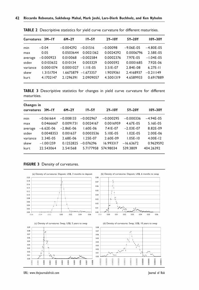
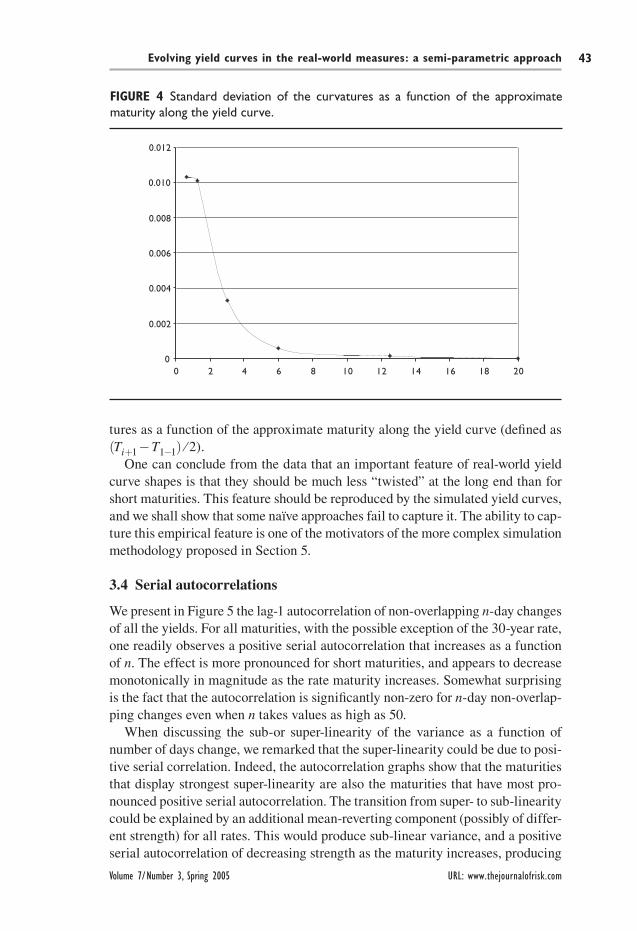
The statistics of the curvature values and of the daily changes in curvature val-ues have been presented in Tables 2 and 3, respectively. Plots of selected densities of the curvatures for several maturities are shown in Figure 3. For future discus-sions, it is important to point out that the distribution of curvatures is much wider at the short end of the curve. Figure 4 shows the standard deviation of the curva-

5 It could be argued that, by the way in which this straight line has been constructed, its slope is very sensitive to small estimation error. While this is true, the one-day variance is the quantity estimated with the largest number of non-overlapping data points and is therefore the most reliable. We checked that very similar results were obtained if the two-day variance, or a combination of the one-day and two-day variances had been used.



TABLE 2 Descripitive statistics for yield curve curvature for different maturities.

Curvatures 3M–1Y 6M–2Y 1Y–5Y 2Y–10Y 5Y–20Y 10Y–30Y

min –0.04 –0.004292 –0.01516 –0.00098 –9.06E-05 –4.80E-05max 0.05 0.0503644 0.0021362 0.0024292 0.0006796 2.58E-05average –0.000923 0.010068 –0.002584 0.0002376 7.97E-05 –1.04E-05stdev 0.0103632 0.010134 0.003329 0.000592 0.0001685 7.92E-06variance 0.0001074 0.0001027 1.11E-05 3.51E-07 2.84E-08 6.27E-11skew 1.3151704 1.6675879 –1.673357 1.9059361 2.4168937 –0.211149kurt 4.1702147 2.1296391 2.0909057 4.5001319 4.6589933 0.6917889

TABLE 3 Descripitive statistics for changes in yield curve curvature for different maturities.

Changes incurvatures 3M–1Y 6M–2Y 1Y–5Y 2Y–10Y 5Y–20Y 10Y–30Y

min –0.061664 –0.008133 –0.002967 –0.000295 –0.000336 –4.94E-05max 0.0466667 0.0091731 0.0024167 0.0016959 4.67E-05 5.16E-05average –6.62E-06 –2.86E-06 1.60E-06 7.41E-07 –2.03E-07 8.82E-09stdev 0.0048353 0.001637 0.0003536 5.10E-05 1.02E-05 2.00E-06variance 2.34E-05 2.68E-06 1.25E-07 2.60E-09 1.05E-10 4.00E-12skew –1.001259 0.1252825 –0.076296 16.993317 –16.63672 0.9629592kurt 22.543064 2.541568 5.7177958 574.98034 539.3809 404.26392

FIGURE 3 Density of curvatures.

(a) Density of curvatures: Deposit, US$, 3 months to deposit

0.00

0.02

0.04

0.06

0.08

0.10

0.12

0.14

0.16

0.18

0.20

-0.06 -0.04 -0.02 0.00 0.02 0.04 0.06

(b) Density of curvatures: Deposit, US$, 6 months to swap

0.00

0.01

0.02

0.03

0.04

0.05

0.06

0.07

0.08

-0.01 0.00 0.01 0.02 0.03 0.04 0.05 0.06

0.00

0.01

0.02

0.03

0.04

0.05

0.06

0.07

0.08

0.09

-0.0

002

-0.0

001

0.00

00

0.00

01

0.00

02

0.00

03

0.00

04

0.00

05

0.00

06

0.00

07

0.00

08

(d) Density of curvatures: Swap, US$, 10 years to swap(c) Density of curvatures: Swap, US$, 5 years to swap

0.00

0.01

0.02

0.03

0.04

0.05

0.06

0.07

0.08

-0.0

0003

5

-0.0

0003

0

-0.0

0002

5

-0.0

0002

0

-0.0

0001

5

-0.0

0001

0

-0.0

0000

5

0.00

0000

0.00

0005

0.00

0010

0.00

0015



tures as a function of the approximate maturity along the yield curve (defined as (Ti+1 − T1−1) ⁄ 2).

One can conclude from the data that an important feature of real-world yield curve shapes is that they should be much less “twisted” at the long end than for short maturities. This feature should be reproduced by the simulated yield curves, and we shall show that some naïve approaches fail to capture it. The ability to cap-ture this empirical feature is one of the motivators of the more complex simulation methodology proposed in Section 5.

3.4 Serial autocorrelations

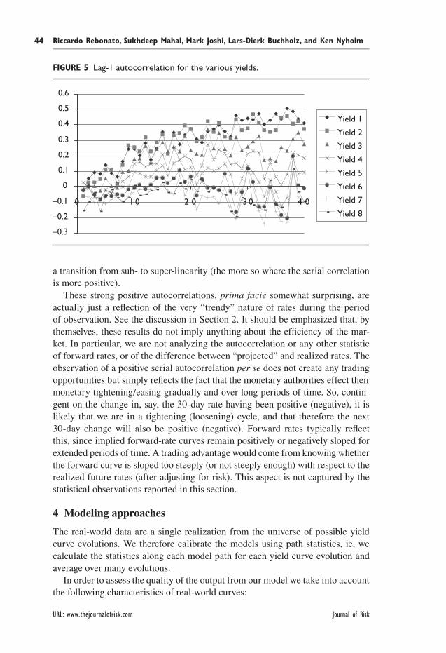
We present in Figure 5 the lag-1 autocorrelation of non-overlapping n-day changes of all the yields. For all maturities, with the possible exception of the 30-year rate, one readily observes a positive serial autocorrelation that increases as a function of n. The effect is more pronounced for short maturities, and appears to decrease monotonically in magnitude as the rate maturity increases. Somewhat surprising is the fact that the autocorrelation is significantly non-zero for n-day non-overlap-ping changes even when n takes values as high as 50.

When discussing the sub-or super-linearity of the variance as a function of number of days change, we remarked that the super-linearity could be due to posi-tive serial correlation. Indeed, the autocorrelation graphs show that the maturities that display strongest super-linearity are also the maturities that have most pro-nounced positive serial autocorrelation. The transition from super- to sub-linearity could be explained by an additional mean-reverting component (possibly of differ-ent strength) for all rates. This would produce sub-linear variance, and a positive serial autocorrelation of decreasing strength as the maturity increases, producing

FIGURE 4 Standard deviation of the curvatures as a function of the approximate maturity along the yield curve.

0

0.002

0.004

0.006

0.008

0.010

0.012

0 2 4 6 8 10 12 14 16 18 20



a transition from sub- to super-linearity (the more so where the serial correlation is more positive).

These strong positive autocorrelations, prima facie somewhat surprising, are actually just a reflection of the very “trendy” nature of rates during the period of observation. See the discussion in Section 2. It should be emphasized that, by themselves, these results do not imply anything about the efficiency of the mar-ket. In particular, we are not analyzing the autocorrelation or any other statistic of forward rates, or of the difference between “projected” and realized rates. The observation of a positive serial autocorrelation per se does not create any trading opportunities but simply reflects the fact that the monetary authorities effect their monetary tightening/easing gradually and over long periods of time. So, contin-gent on the change in, say, the 30-day rate having been positive (negative), it is likely that we are in a tightening (loosening) cycle, and that therefore the next 30-day change will also be positive (negative). Forward rates typically reflect this, since implied forward-rate curves remain positively or negatively sloped for extended periods of time. A trading advantage would come from knowing whether the forward curve is sloped too steeply (or not steeply enough) with respect to the realized future rates (after adjusting for risk). This aspect is not captured by the statistical observations reported in this section.

4 Modeling approaches

The real-world data are a single realization from the universe of possible yield curve evolutions. We therefore calibrate the models using path statistics, ie, we calculate the statistics along each model path for each yield curve evolution and average over many evolutions.

In order to assess the quality of the output from our model we take into account the following characteristics of real-world curves:

FIGURE 5 Lag-1 autocorrelation for the various yields.

–0.3

–0.2

–0.1

0

0.1

0.2

0.3

0.4

0.5

0.6

0 1 0 2 0 3 0 4 0

Yield 1

Yield 2

Yield 3

Yield 4

Yield 5

Yield 6

Yield 7

Yield 8



❑ variance of rates;❑ variance of curvatures;❑ variance of n-day non-overlapping changes;❑ lag-1 autocorrelation of n-day non-overlapping changes; and❑ eigenvalues and eigenvectors.

4.1 A totally non-parametric approach: description

The simplest approach to evolve the current yield curve is to assume that each vector of rate changes is drawn at random (with equal probability) from the 2,134 observed vector changes. More precisely, let {yi

k} denote the vector of (the loga-rithm of) rates6 on day k, k = 1, 2, … , N, and {yi

N}, i = 1, 2, … , 8 be the vector of rates describing today’s yield curve. Let ∆yi

k, k = 2, 3, … , N be the change in the i th rate between day k and day k −1:

(3)∆y y yik

ik

ik= − −1

Suppose that we want to evolve the yield curve M days forward. Draw M indepen-dent variates, Ur , r = 1, 2, … , M, from the uniform discrete [1 N] distribution.7 In the naïve approach, the future yield curve that will prevail M days after today is simply given by8

(4)y y yiN M

iN

iU

r M

r+

=

= + ∑ ∆1,

By drawing a whole synchronous vector this procedure preserves whatever co-dependence structure the original data might show across maturities. If the increments were iid, the procedure would asymptotically fully capture both the serial autocorrelation structure (or rather, the lack thereof) and the cross-sectional co-dependence. For general increments, however, this is no longer true. The analysis below shows that the deviation form iid behavior (which could already be expected in the light of the data description in Section 2) is sufficiently strong to make the procedure unsatisfactory. Nonetheless, it is interesting to point out how many features even this naïve approach does recover. In particular, it is straight-

6 The same procedure can be used for absolute or percentage changes, and the symbol y can refer either to the rate or to its logarithm. In the study we have used percentage changes to ensure positivity, but to lighten the exposition we refer to “rates” in the text. See, however, the discussion in Section 6.7 In the uniform discrete [1 N] distribution all integers between 1 and N have the identical mass probability of occurrence of 1 ⁄N.8 A remark on notation: to avoid the proliferation of symbols, we use the use the same symbol, y, to denote past and present observed rates and future simulated rates. Ambiguity is avoided thanks to the range of the superscript: the first historical vector of rates in our database is labeled by the superscript 1. Since we have N distinct days of data the current curve has the superscript N. Future rates are identified by having a superscript greater than N.



forward to show that all the eigenvectors and eigenvalues of the sample data are fully recovered by the naïve procedure, as are all the unconditional one-day variances. This inserts a strong caveat regarding the validity of those procedures that invoke orthogonalization of the covariance matrix (and retention of a small number of eigenvectors).

In the discussion presented below we refer to this method as the random-sampling approach.

4.1.1 Positive features and shortcomings of the random-sampling approachGiven a time series of changes of a set of time-indexed data, it is obviously always possible to construct and orthogonalize a covariance matrix. In many fields (eg, interest rate modeling) it has become customary to work with the resulting eigen-vectors and eigenvalues (for instance, in the LIBOR-market-model context, this is often done by calibrating the model-implied correlation matrix among forward rates to the corresponding statistical quantity). Working with the full eigen system has in practice often proven to be too computationally expensive. The computa-tional difficulties associated with multifactor no-arbitrage pricing have therefore forced the modeler to drop many of the eigenvectors and to rescale the few pre-served eigenvalues in such a way as to recover some important quantities (eg, the prices of caplets). It has been claimed by Longstaff et al (2000) that the inability to work with a full-factor model can have very adverse financial consequences (their controversial paper on this topic in the context of Bermudan swaptions was titled “Throwing away a billion dollars”). It has therefore become customary to consider

FIGURE 6 Yield curves obtained using the naïve method.

3.00

5.00

7.00

9.00

11.00

13.00

15.00

0 5 10 15 20 25 30

0360720108014401800

(a)

2.00

3.00

4.00

5.00

6.00

7.00

8.00

9.00

10.00

11.00

12.00

0 5 10 15 20 25 30

0360720108014401800

(c)

1.00

2.00

3.00

4.00

5.00

6.00

7.00

8.00

9.00

0 5 10 15 20 25 30

0360720108014401800

(b)

3.00

4.00

5.00

6.00

7.00

8.00

9.00

10.00

11.00

12.00

13.00

0 5 10 15 20 25 30

0360720108014401800

(d)



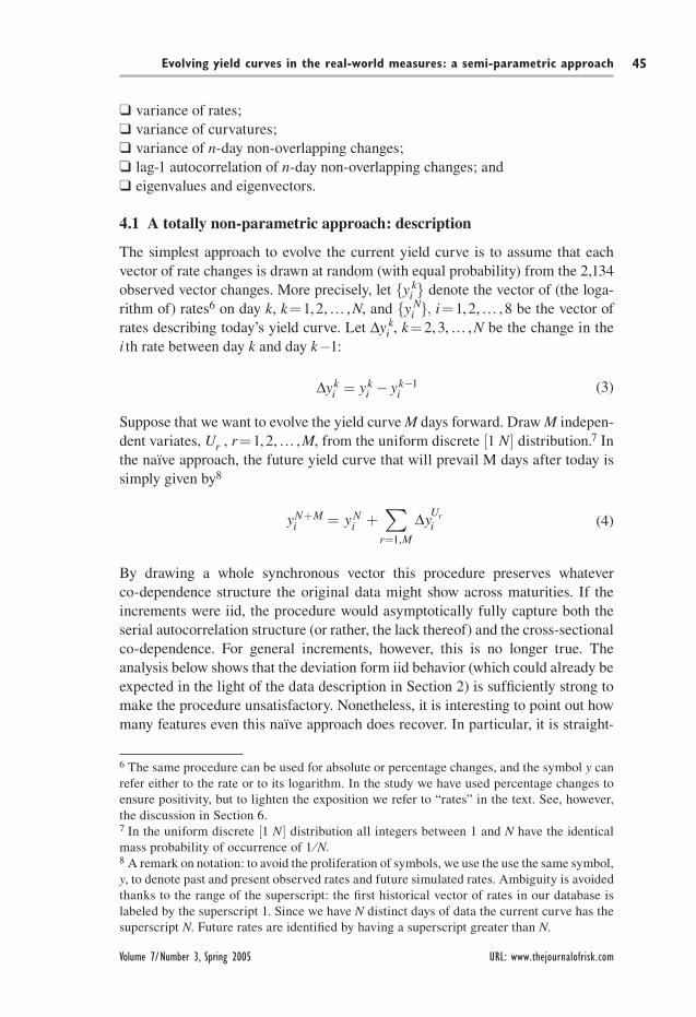
the ability to work with the full dimensionality of the eigenvectors almost like a Holy Grail. The analysis presented below shows how little is actually achieved in terms of realistic modeling of the yield curve, even when all the eigenvectors and eigenvalues are correctly recovered. In particular, Figure 6, which displays a few typical yield curves evolved by the random-sampling method over a period of five years, shows the qualitatively unsatisfactory nature of the procedure: it is dif-ficult, for instance, to find “convincing” a yield curve that drops from 10% to 7% for maturities up to one year, and then rises to above 13% for two-year yields (see

FIGURE 7 Eigenvalues for the real data (empirical), the naïve method (random), the spring method (spring) and the spring-and-box method (box).

Eigenvalues

0

0.0001

0.0002

0.0003

0.0004

0.0005

0.0006

0.0007

0.0008

0.0009

0 2 4 6 8 1 0

Empirical

Random

Spring

Box

FIGURE 8 The first eigenvector for the real data (empirical), the naïve method (random), the spring method (spring) and the spring-and-box method (box).

First eigenvector

–0.7

–0.6

–0.5

–0.4

–0.3

–0.2

–0.1

01 2 3 4 5 6 7 8

Empirical

Random

Spring

Box



Figure 6a). Yet, the naïve procedure proposed above recovers (asymptotically) exactly all the eigenvalues and eigenvectors (see Figures 7–10). This is because the vectors of changes are exactly the same as in the real world, and, if the evolution of the yield curve is sufficiently long, they will all be represented with the same fre-quency as in the real-world data set. Therefore, the model covariance matrix will asymptotically be the same as the empirical one, and so too will be its eigenvalues and eigenvectors. Clearly, any single realization of the yield curve evolution will

FIGURE 9 The second eigenvector for the real data (empirical), the naïve method (random), the spring method (spring) and the spring-and-box method (box).

Second eigenvector

-0.4

-0.2

0

0.2

0.4

0.6

0.8

1 2 3 4 5 6 7 8

Empirical

Random

Spring

Box

FIGURE 10 The third eigenvector for the real data (empirical), the naïve method (random), the spring method (spring) and the spring-and-box method (box).

Third eigenvector

–0.8

–0.6

–0.4

–0.2

0

0.2

0.4

0.6

0.8

1 2 3 4 5 6 7 8

Empirical

Random

Spring

Box



produce different eigenvectors and eigenvalues, but this is nothing more than the effect of a finite-size sampling.

By the same token, every statistical quantity that does not depend on the order along the time axis of the quantities used for its computation will be recovered exactly by the non-parametric approach. Therefore, the one-day variance and the correlation matrix will also be exactly recovered. Crucially, the same is not true, however, for the many-day variance, where serial correlation becomes important.

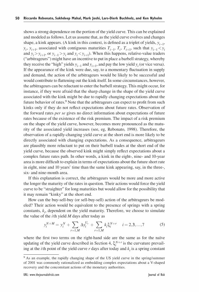
Apart from the “implausible” look of the yield curves generated by the random-sampling method, the shortcomings of the approach just introduced were that the distribution of curvatures, the serial autocorrelation, and the many-day variances turned out to be at odds with the corresponding real-world quantities (see Figure 11). In particular, the serial autocorrelation was, within statistical noise, zero (not surprisingly, given the method of sampling), and the many-day variance was observed to grow almost linearly with the number, m, of days in the change. Both these features point to the fact that the most important mis-specification of the approach is to be found in the fact that it implies, by construction, independent increments.

5 A financial and computational model

5.1 Arbitrageurs and the curvature of the yield curve: the barbell mechanism

In order to obviate the shortcomings associated with the naïve approach described above, a simple mechanism can be introduced. The shapes of the yield curves produced using the simple approach show that one of its unsatisfactory features is the presence of “kinks” and pronounced changes in the slope for long maturities. In reality, the width of the statistical distribution of curvatures, as discussed above,

FIGURE 11 Lag-1 auto-correlation with the naïve sampling.

Lag-1 serial autocorrelation (random)

–0.6

–0.4

–0.2

0

0.2

0.4

0.6

Yield 1

Yield 2

Yield 3

Yield 4

Yield 5

Yield 6

Yield 7

Yield 8

0 10 20 30 40 50



shows a strong dependence on the portion of the yield curve. This can be explained and modeled as follows. Let us assume that, as the yield curve evolves and changes shape, a kink appears. (A kink in this context, is defined as a triplet of yields, yi−1, yi , yi+1, associated with contiguous maturities Ti−1, Ti , Ti+1, such that yi−1 < yi and yi > yi+1, or yi−1 > yi and yi < yi+1). When this happens, relative-value traders (“arbitrageurs”) might have an incentive to put in place a barbell strategy, whereby they receive the “high” yields yi−1 and yi+1, and pay the low yield yi (or vice versa). If the appearance of the kink were due, say, to a momentary fluctuation in supply and demand, the action of the arbitrageurs would be likely to be successful and would contribute to flattening out the kink itself. In some circumstances, however, the arbitrageurs can be reluctant to enter the barbell strategy. This might occur, for instance, if they were afraid that the sharp change in the shape of the yield curve associated with the kink might be due to rapidly changing expectations about the future behavior of rates.9 Note that the arbitrageurs can expect to profit from such kinks only if they do not reflect expectations about future rates. Observation of the forward rates per se gives no direct information about expectations of future rates because of the existence of the risk premium. The impact of a risk premium on the shape of the yield curve, however, becomes more pronounced as the matu-rity of the associated yield increases (see, eg, Rebonato, 1998). Therefore, the observation of a rapidly-changing yield curve at the short end is more likely to be directly associated with changing expectations. As a consequence, arbitrageurs are plausibly more reluctant to put on their barbell trades at the short end of the yield curve, because the observed kink might simply reflect expectations about a complex future rates path. In other words, a kink in the eight-, nine- and 10-year area is more difficult to explain in terms of expectations about the future short rate in eight, nine and 10 years’ time than the same kink appearing, say, in the three-, six- and nine-month area.

If this explanation is correct, the arbitrageurs would be more and more active the longer the maturity of the rates in question. Their actions would force the yield curve to be “straighter” for long maturities but would allow for the possibility that it may remain “kinky” at the short end.

How can the buy-sell-buy (or sell-buy-sell) action of the arbitrageurs be mod-eled? Their action would be equivalent to the presence of springs with a spring constants, ki, dependent on the yield maturity. Therefore, we choose to simulate the value of the i th yield M days after today as

(5)y y y k iiN M

iN

iU

r Mi i

N r

r M

r+

=

+

=

= + + =∑ ∑∆1 1

2, ,

,ξ 33 7, ,…

where the first two terms on the right-hand side are the same as for the naïve updating of the yield curve described in Section 4, ξi

N+r is the curvature prevail-ing at the i th point of the yield curve r days after today and ki is a spring constant

9 As an example, the rapidly changing shape of the US yield curve in the spring/summer of 2001 was commonly rationalized as embedding complex expectations about a V-shaped recovery and the concomitant actions of the monetary authorities.



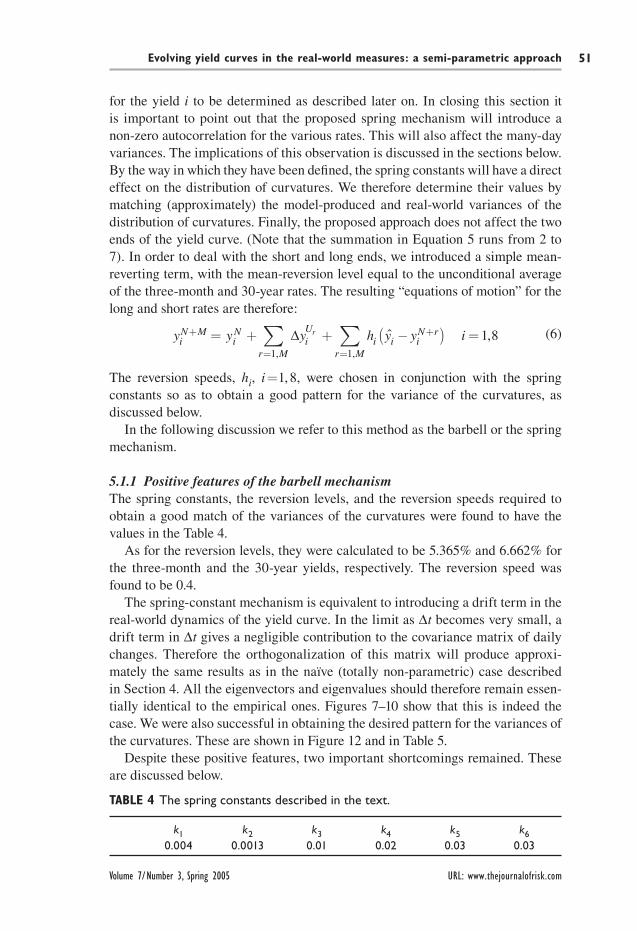
for the yield i to be determined as described later on. In closing this section it is important to point out that the proposed spring mechanism will introduce a non-zero autocorrelation for the various rates. This will also affect the many-day variances. The implications of this observation is discussed in the sections below. By the way in which they have been defined, the spring constants will have a direct effect on the distribution of curvatures. We therefore determine their values by matching (approximately) the model-produced and real-world variances of the distribution of curvatures. Finally, the proposed approach does not affect the two ends of the yield curve. (Note that the summation in Equation 5 runs from 2 to 7). In order to deal with the short and long ends, we introduced a simple mean-reverting term, with the mean-reversion level equal to the unconditional average of the three-month and 30-year rates. The resulting “equations of motion” for the long and short rates are therefore:

(6)y y y h y yiN M

iN

iU

r Mi i i

N r

r M

r+

=

+

=

= + + −( )∑ ∑∆1 1, ,

ˆ ,i = 1 8

The reversion speeds, hi, i =1, 8, were chosen in conjunction with the spring constants so as to obtain a good pattern for the variance of the curvatures, as discussed below.

In the following discussion we refer to this method as the barbell or the spring mechanism.

5.1.1 Positive features of the barbell mechanismThe spring constants, the reversion levels, and the reversion speeds required to obtain a good match of the variances of the curvatures were found to have the values in the Table 4.

As for the reversion levels, they were calculated to be 5.365% and 6.662% for the three-month and the 30-year yields, respectively. The reversion speed was found to be 0.4.

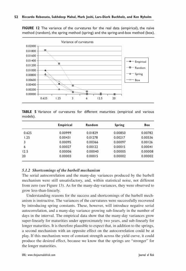
The spring-constant mechanism is equivalent to introducing a drift term in the real-world dynamics of the yield curve. In the limit as ∆t becomes very small, a drift term in ∆t gives a negligible contribution to the covariance matrix of daily changes. Therefore the orthogonalization of this matrix will produce approxi-mately the same results as in the naïve (totally non-parametric) case described in Section 4. All the eigenvectors and eigenvalues should therefore remain essen-tially identical to the empirical ones. Figures 7–10 show that this is indeed the case. We were also successful in obtaining the desired pattern for the variances of the curvatures. These are shown in Figure 12 and in Table 5.

Despite these positive features, two important shortcomings remained. These are discussed below.

TABLE 4 The spring constants described in the text.

k1 k2 k3 k4 k5 k6 0.004 0.0013 0.01 0.02 0.03 0.03



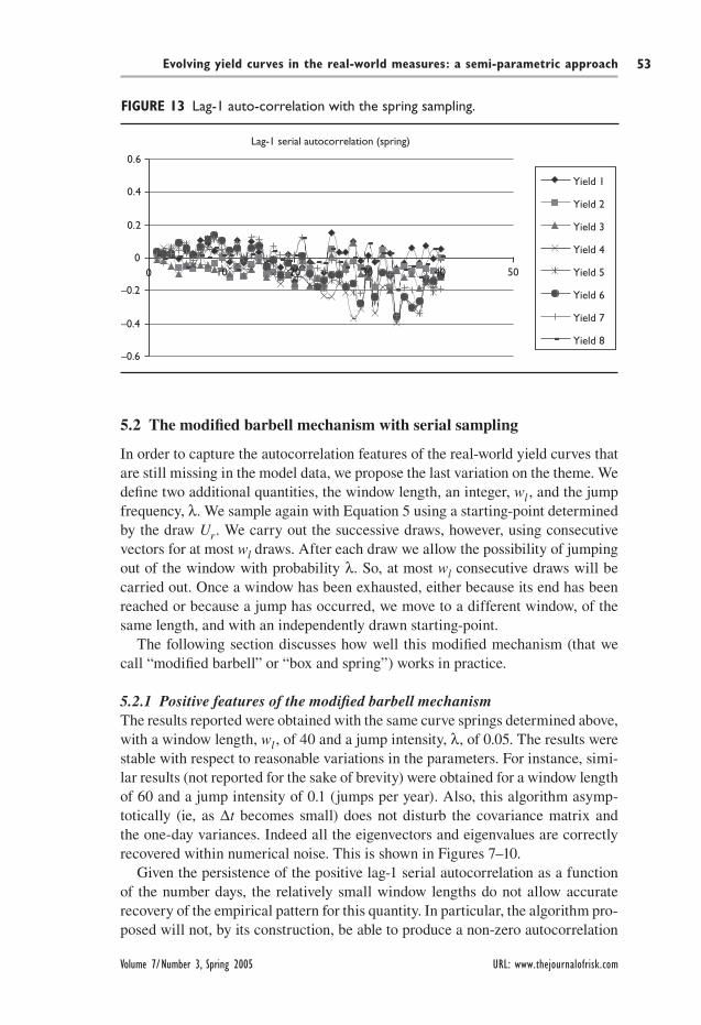
5.1.2 Shortcomings of the barbell mechanismThe serial autocorrelation and the many-day variances produced by the barbell mechanism were still unsatisfactory, and, within statistical noise, not different from zero (see Figure 13). As for the many-day-variances, they were observed to grow less-than-linearly.

Understanding reasons for the success and shortcomings of the barbell mech-anism is instructive. The variances of the curvatures were successfully recovered by introducing spring constants. These, however, will introduce negative serial autocorrelation, and a many-day variance growing sub-linearly in the number of days in the interval. The empirical data show that the many-day variances grow super-linearly for maturities under approximately two years, and sub-linearly for longer maturities. It is therefore plausible to expect that, in addition to the springs, a second mechanism with an opposite effect on the autocorrelation could be at play. If this mechanism were of constant strength across the yield curve, it could produce the desired effect, because we know that the springs are “stronger” for the longer maturities.

FIGURE 12 The variance of the curvatures for the real data (empirical), the naïve method (random), the spring method (spring) and the spring-and-box method (box).

Variance of curvatures

0.00200

0.00000

0.00400

0.00600

0.00800

0.01000

0.01200

0.01400

0.01600

0.01800

0.02000

0.625 1.25 3 6 12.5 20

Empirical

Random

Spring

Box

TABLE 5 Variance of curvatures for different maturities (empirical and various models).

Empirical Random Spring Box

0.625 0.00999 0.01829 0.00850 0.00782 1.25 0.00431 0.01278 0.00217 0.00536 3 0.00095 0.00366 0.00097 0.00126 6 0.00027 0.00122 0.00015 0.0004112.5 0.00006 0.00040 0.00005 0.0000820 0.00003 0.00015 0.00002 0.00002



5.2 The modified barbell mechanism with serial sampling

In order to capture the autocorrelation features of the real-world yield curves that are still missing in the model data, we propose the last variation on the theme. We define two additional quantities, the window length, an integer, wl , and the jump frequency, λ. We sample again with Equation 5 using a starting-point determined by the draw Ur. We carry out the successive draws, however, using consecutive vectors for at most wl draws. After each draw we allow the possibility of jumping out of the window with probability λ. So, at most wl consecutive draws will be carried out. Once a window has been exhausted, either because its end has been reached or because a jump has occurred, we move to a different window, of the same length, and with an independently drawn starting-point.

The following section discusses how well this modified mechanism (that we call “modified barbell” or “box and spring”) works in practice.

5.2.1 Positive features of the modified barbell mechanismThe results reported were obtained with the same curve springs determined above, with a window length, wl , of 40 and a jump intensity, λ, of 0.05. The results were stable with respect to reasonable variations in the parameters. For instance, simi-lar results (not reported for the sake of brevity) were obtained for a window length of 60 and a jump intensity of 0.1 (jumps per year). Also, this algorithm asymp-totically (ie, as ∆t becomes small) does not disturb the covariance matrix and the one-day variances. Indeed all the eigenvectors and eigenvalues are correctly recovered within numerical noise. This is shown in Figures 7–10.

Given the persistence of the positive lag-1 serial autocorrelation as a function of the number days, the relatively small window lengths do not allow accurate recovery of the empirical pattern for this quantity. In particular, the algorithm pro-posed will not, by its construction, be able to produce a non-zero autocorrelation

FIGURE 13 Lag-1 auto-correlation with the spring sampling.

Lag-1 serial autocorrelation (spring)

–0.6

–0.4

–0.2

0

0.2

0.4

0.6

0

Yield 1

Yield 2

Yield 3

Yield 4

Yield 5

Yield 6

Yield 7

Yield 8

10 20 30 40 50



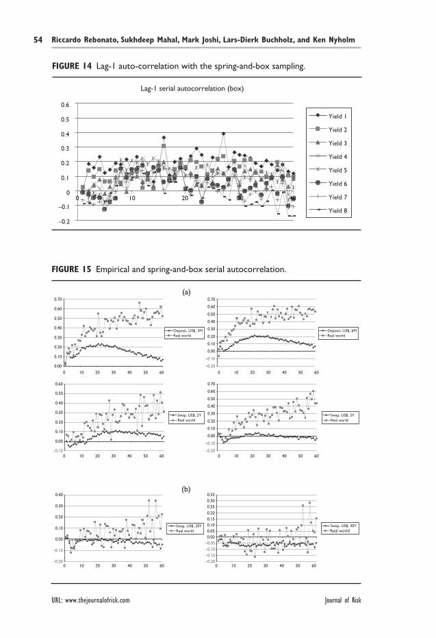
FIGURE 14 Lag-1 auto-correlation with the spring-and-box sampling.

Lag-1 serial autocorrelation (box)

–0.2

–0.1

0

0.1

0.2

0.3

0.4

0.5

0.6

Yield 1

Yield 2

Yield 3

Yield 4

Yield 5

Yield 6

Yield 7

Yield 8

0 10 20 30 40

FIGURE 15 Empirical and spring-and-box serial autocorrelation.

0.00

0.10

0.20

0.30

0.40

0.50

0.60

0.70

Deposit, US$, 3MReal world

–0.20

–0.10

0.00

0.10

0.20

0.30

0.40

0.50

0.60

0.70

Deposit, US$, 6MReal world

–0.10

0.00

0.10

0.20

0.30

0.40

0.50

0.60

Swap, US$, 2YReal world

–0.20

–0.10

0.00

0.10

0.20

0.30

0.40

0.50

0.60

0.70


0 10 20 30 40 50 60 0 10 20 30 40 50 60

0 10 20 30 40 50 60 0 10 20 30 40 50 60

(a)

–0.20

–0.10

0.00

0.10

0.20

0.30

0.40


–0.20 –0.15 –0.10 –0.05 0.000.050.100.150.200.250.300.35

Real world

0 10 20 30 40 50 60 0 10 20 30 40 50 60

Swap, US$, 30Y

(b)



for changes of more than wl days. Nonetheless, Figure 14 shows that the modi-fied barbell mechanism is certainly an improvement on the random or the simple spring procedures. For greater clarity the empirical and box-and-spring serial autocorrelation are also shown in Figure 15.

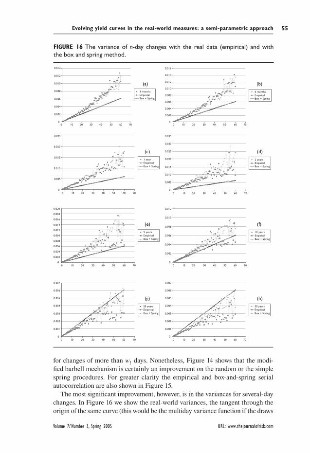
The most significant improvement, however, is in the variances for several-day changes. In Figure 16 we show the real-world variances, the tangent through the origin of the same curve (this would be the multiday variance function if the draws

FIGURE 16 The variance of n-day changes with the real data (empirical) and with the box and spring method.

00 10 20 30 40 50 60 70

0 10 20 30 40 50 60 70

0 10 20 30 40 50 60 70

0 10 20 30 40 50 60 70

0 10 20 30 40 50 60 70

0 10 20 30 40 50 60 70

0 10 20 30 40 50 60 70 0 10 20 30 40 50 60 70

0.002

0.004

0.006

0.008

0.010

0.012

0.014

3 monthsEmpiricalBox + Spring

0

0.002

0.004

0.006

0.008

0.010

0.012

0.014

0.016

6 monthsEmpiricalBox + Spring

0

0.005

0.010

0.015

0.020

0.025

1 yearEmpiricalBox + Spring

0

0.005

0.010

0.015

0.020

0.025

0.030

0.035

2 yearsEmpiricalBox + Spring

0

0.002

0.004

0.006

0.008

0.010

0.012

0.014

0.016

0.018

0.020


0

0.002

0.004

0.006

0.008

0.010

0.012


0

0.001

0.002

0.003

0.004

0.005

0.006

0.007


0

0.001

0.002

0.003

0.004

0.005

0.006

0.007


(a) (b)

(c) (d)

(e) (f)

(g) (h)



were iid), and the model multiday variance obtained with the spring and box mechanism. Note how the model variances switch from growing super-linearly to growing sub-linearly, in agreement with the real-world data.

Qualitatively, the consecutive sampling within each box is sufficient to create a sufficient degree of serial autocorrelation to more than compensate for the neg-ative autocorrelation introduced by the spring mechanism. These two features used together with the random sampling appear to describe to a satisfactory degree the dynamics of the real-world yield curve.

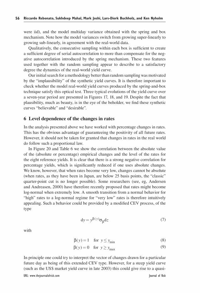
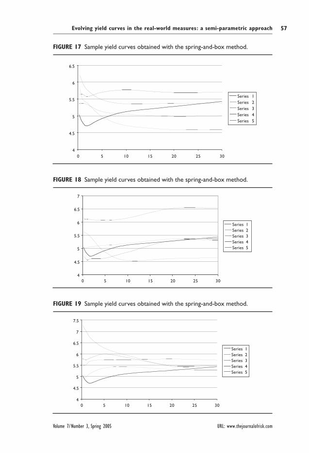
Our initial search for a methodology better than random sampling was motivated by the “implausibility” of the synthetic yield curves. It is therefore important to check whether the model real-world yield curves produced by the spring-and-box technique satisfy this optical test. Three typical evolutions of the yield curve over a seven-year period are presented in Figures 17, 18, and 19. Despite the fact that plausibility, much as beauty, is in the eye of the beholder, we find these synthetic curves “believable” and “desirable”.

6 Level dependence of the changes in rates

In the analysis presented above we have worked with percentage changes in rates. This has the obvious advantage of guaranteeing the positivity of all future rates. However, it should not be taken for granted that changes in rates in the real world do follow such a proportional law.

In Figure 20 and Table 6 we show the correlation between the absolute value of the (absolute or percentage) empirical changes and the level of the rates for the eight reference yields. It is clear that there is a strong negative correlation for percentage yields, which is significantly reduced if one uses absolute changes. We know, however, that when rates become very low, changes cannot be absolute (when rates, as they have been in Japan, are below 25 basis points, the “classic” quarter-point cut is no longer possible). Some researchers (see, eg, Andersen and Andreasen, 2000) have therefore recently proposed that rates might become log-normal when extremely low. A smooth transition from a normal behavior for “high” rates to a log-normal regime for “very low” rates is therefore intuitively appealing. Such a behavior could be provided by a modified CEV process, of the type

(7)d dy y zy= ββσ( )

with

(8)

(9)

β

β

( )

( )min

max

y y y

y y y

= ≤

= ≥

1

0

for

for

In principle one could try to interpret the vector of changes drawn for a particular future day as being of this extended CEV type. However, for a steep yield curve (such as the US$ market yield curve in late 2003) this could give rise to a quasi-



FIGURE 17 Sample yield curves obtained with the spring-and-box method.

4

4.5

5

5.5

6

6.5

0 5 10 15 20 25 30

Series 1Series 2Series 3Series 4Series 5


4

4.5

5

5.5

6

6.5

7

0 5 10 15 20 25 30



4

4.5

5

5.5

6

6.5

7

7.5

0 5 10 15 20 25 30




lognormal behavior at the short end and to an almost-normal behavior at the long end. Incidentally, to give an idea of the complexity of the empirical studies, Ait-Sahalia (1996) and Chan et al (1992) find evidence that the exponent should be greater than 1. Perhaps it would be interesting to repeat some of the econometric investigations carried out in the past with recent market data, which would contain the exceptionally low rates encountered in US dollars, euros, Japanese yen and, to some extent, UK pounds.

These complications could be handled with some care, but, given the non-process-based approach that we have chosen to follow in this paper, we prefer to leave the analysis at this stage.

7 Discussion and conclusions

We have shown in this paper how the real-world evolution of the yield curve can be simulated in a simple and effective semi-parametric way. The proposed procedure

FIGURE 20 Correlation between the absolute value of the (absolute or percentage) empirical changes and the level of the rates for the eight reference yields.

–0.60000

–0.50000

–0.40000

–0.30000

–0.20000

–0.10000

0.00000

0.10000

3m 6m 1y 2y 5y 10y 20y 30y

Percentage

Absolute

TABLE 6 Correlation between the absolute value of the (absolute or percentage) empirical changes and the level of rates for the eight reference yields.

Percentage Absolute

3 months –0.25930 0.04227 6 months –0.35212 0.01889 1 year –0.47963 –0.05670 2 years –0.48984 –0.08982 5 years –0.39558 –0.1271810 years –0.25171 –0.0709820 years –0.12260 0.0065530 years –0.06846 0.01371



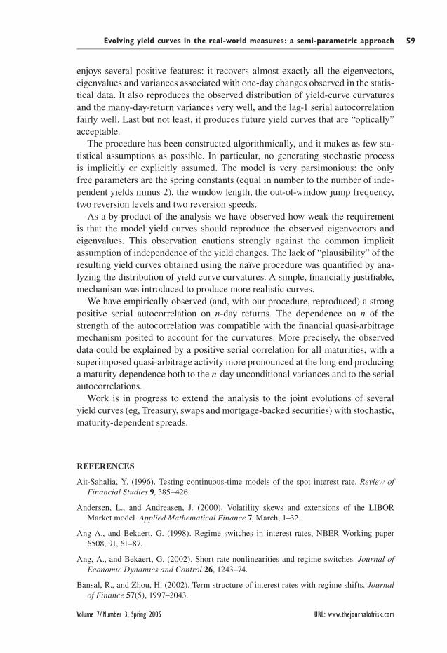
enjoys several positive features: it recovers almost exactly all the eigenvectors, eigenvalues and variances associated with one-day changes observed in the statis-tical data. It also reproduces the observed distribution of yield-curve curvatures and the many-day-return variances very well, and the lag-1 serial autocorrelation fairly well. Last but not least, it produces future yield curves that are “optically” acceptable.

The procedure has been constructed algorithmically, and it makes as few sta-tistical assumptions as possible. In particular, no generating stochastic process is implicitly or explicitly assumed. The model is very parsimonious: the only free parameters are the spring constants (equal in number to the number of inde-pendent yields minus 2), the window length, the out-of-window jump frequency, two reversion levels and two reversion speeds.

As a by-product of the analysis we have observed how weak the requirement is that the model yield curves should reproduce the observed eigenvectors and eigenvalues. This observation cautions strongly against the common implicit assumption of independence of the yield changes. The lack of “plausibility” of the resulting yield curves obtained using the naïve procedure was quantified by ana-lyzing the distribution of yield curve curvatures. A simple, financially justifiable, mechanism was introduced to produce more realistic curves.

We have empirically observed (and, with our procedure, reproduced) a strong positive serial autocorrelation on n-day returns. The dependence on n of the strength of the autocorrelation was compatible with the financial quasi-arbitrage mechanism posited to account for the curvatures. More precisely, the observed data could be explained by a positive serial correlation for all maturities, with a superimposed quasi-arbitrage activity more pronounced at the long end producing a maturity dependence both to the n-day unconditional variances and to the serial autocorrelations.

Work is in progress to extend the analysis to the joint evolutions of several yield curves (eg, Treasury, swaps and mortgage-backed securities) with stochastic, maturity-dependent spreads.

REFERENCES

Ait-Sahalia, Y. (1996). Testing continuous-time models of the spot interest rate. Review of Financial Studies 9, 385–426.

Andersen, L., and Andreasen, J. (2000). Volatility skews and extensions of the LIBOR Market model. Applied Mathematical Finance 7, March, 1–32.

Ang A., and Bekaert, G. (1998). Regime switches in interest rates, NBER Working paper 6508, 91, 61–87.

Ang, A., and Bekaert, G. (2002). Short rate nonlinearities and regime switches. Journal of Economic Dynamics and Control 26, 1243–74.

Bansal, R., and Zhou, H. (2002). Term structure of interest rates with regime shifts. Journal of Finance 57(5), 1997–2043.



Banzal, R., Tauchen, G., and Zhou, H. (2003). Regime-shifts, risk premiums in the term structure, and the business cycle. Working paper, Duke University.

Black, F., Derman, E., and Toy, W. (1990). A one-factor model of interest rates and its appli-cation to Treasury bond options. Financial Analyst Journal 1990, 33–339.

Brennan, M. J., and Schwartz, E. S. (1982). an equilibrium model of bond pricing and a test of market efficiency. Journal of Financial Quantitative Analysis 17, 301–29.

Brigo, F., and Mercurio, D. (2001). Interest-Rate Models – Theory and Practice. Springer Verlag, Berlin, Heidelberg.

Campbell, J.Y., and Shiller, R. J. (1987). Cointegration and tests of present value models. Journal of Political Economy 95(5), 1062–88.

Chan, K. C., Karolyi, G. A., Longstaff, F. A., and Sanders, A. B. (1992). An empirical com-parison of alternative models of the short-term interest rate. Journal of Finance 57, May.

Cox J., Ingersoll, J. E., and Ross, S. A. (1985). A theory of the term structure of interest rates Econometrica 53, 385–407.

Dai, Q., Singleton, K. J., and Yang, W. (2003). Regime shifts in a dynamic term structure model of U.S. Treasury Bond yields. Working paper, Stern School of Business.

Driffill, J., Kenc, T., and Sola, M. (2003). An empirical examination of term structure model with regime shifts. Working paper, Birkbeck College, University of London.

Evans, D. D. (2003). Real risk, inflation risk, and the term structure. The Economic Journal 113, 345–89.

Joshi, M., and Rebonato, R. (2003). A stochastic-volatility extension of the LIBOR market model. Quantitative Finance, accepted for publication.

Garcia, P., and Perron, P. (1996). An analysis of the real interest rate under regime shifts. Review of Economics and Statistics 78, 111–25.

Glasserman, P., and Kou, S. G. (2000). The term structure of simple forward rates with jump risk. Working paper, Columbia University.

Gray, S. F. (1996). Modeling the distribution of interest rates as a regime-switching process. Journal of Financial Economics 42, 27–62.

Hall, A. D., Anderson, H. M., and Granger, W. J. (1992). A cointegration analysis of Treasury Bill yields. Review of Economics and Statistics 74(1). 116–26.

Hamilton, J. (1989). A new approach to the economic analysis of non-stationary time series and the business cycle. Econometrica 57, 357–84.

Heath, D., Jarrow, R. A., and Morton, A. (1989). Bond pricing and the term structure of inter-est rates: a new methodology. Working paper (revised edition), Cornell University.

Ho, T. S. Y., and Lee, S-B. (1986). Term structure movements and pricing interest rate contin-gent claims. Journal of Finance 41, 1011–28.

Hogan, M. (1993). Problems in certain two-factor term structure models. Annals of Applied Probability 3, 576–91.

Hughston, L. (2000). The New Interest Rate Models, ed Lane Hughston, Risk Books, London.

Hughston, L., and Brody, D. C. (2000). Modern theory of interest rates, with extensions to foreign exchange, inflation and credit. Working paper, Kings College.



Hull, J., and White, A. (1990). Pricing interest rate securities. Review of Financial Studies 3, 573–92.

Jorion, P. (1997). Value at Risk. Irving Professional Publishing, Chicago, London, Singapore.

Kugler, P. (1990). The term structure of Euro interest rates and rational expectations. Journal of International Money and Finance 9, 234–44.

Lanne, M. (2000). Near unit roots, cointegration, and the term structure of interest rates. Journal of Applied Econometrics 15, 513–29.

Longstaff, F. A., and Schwartz, E. S. (1992). Interest rate volatility and the term structure: a two-factor general equilibrium model. Journal of Finance 47, 1259–82.

Longstaff, F. A., Santa-Clara, P., and Schwartz, E. S. (2000). Throwing away a billion dol-lars: The cost of sub-optimal exercise strategies in the swaptions markets. Working paper, UCLA, presented at the ICBI Risk Conference – Geneva (2000).

Naik, V., and Lee, M. H. (1997). Yield curve dynamics with discrete shifts in economic regimes: theory and estimation. Working paper, Faculty of Commerce, University of British Columbia.

Martellini, L., and Priaulet, P. (2001). Fixed-Income Securities. John Wiley, Chichester.

Morton, A. (1996). PhD thesis, Cornell University.

Prigent, J-L., Renault, O., and Scaillet, O. (2000). An empirical investigation in credit spread indices. London School of Economics, Discussion Paper 363.

Rebonato, R. (2002). Modern Pricing of Interest-rate Derivatives: The LIBOR Market Model and Beyond, Chapter 1. Princeton University Press, Princeton, New Jersey.

Rebonato, R., and Cooper, I. (1995). Limitations of simple two-factor interest rate models. Journal of Financial Engineering 5, 1–16.

Stanton, R. (1997). A non-parametric model of term structure dynamics and the market price of interest rate risk. Journal of Finance 52, 1973–2002.

Vasicek, O. (1977). an equilibrium characterization of the term structure. Journal of Financial Economics 5, 177–88.


Documents

Evolving yield curves in the real-world measures: a …quantlabs.net/academy/download/free_quant_instituitional_books... · 30 Riccardo Rebonato, Sukhdeep Mahal, Mark Joshi, Lars-Dierk