Embed Size (px)
Citation preview
Copyright © 2014 The eVSM Group, All Rights Reserved
eVSM Contact:
Jay Shah – [email protected]
eVSM Value Stream
Mapping Workshop for
Processing Industries

Copyright © 2014 The eVSM Group, All Rights Reserved
Copyright © 2014 The eVSM Group, All Rights Reserved
Part I: eVSM Overview 5
Lean & eVSM Slides 6
Working with Quick Stencils in eVSM v7 18
Part II: Plant Level Mapping 21
Quick Processing Slides 22
Process Industries VSM Terms 25
Enriched Grain - Plant 30
Plant Templates 33
eVSM Plant Workshop 39
eVSM Rework 43
eVSM Packaging 47
eVSM ByProduct 51
Quick Processing Tutorial 55
eVSM Multi-Station Workshop 82
eVSM - Improvements Workshop 83
Chicago Rice – Resource Modeling 84
Resource Templates 85
eVSM - Resource Workshop 89
Part III: Inbound and Outbound Maps 93
Enriched Grain - Inbound 94
Inbound Network Templates 99
eVSM Inbound Workshop 105
Enriched Grain - Outbound 108
Outbound Network Templates 111
Copyright © 2014 The eVSM Group, All Rights Reserved
eVSM Outbound Workshop 119
Part IV: Linking Maps Together 123
eVSM Extras 127
Units Handling 128
Using Gadgets to Visualize Data 132
Spaghetti Diagram Tutorial 136

Copyright © 2014 The eVSM Group, All Rights Reserved

Copyright © 2014 The eVSM Group, All Rights Reserved 4
Copyright © 2014 The eVSM Group, All Rights Reserved
Part I: eVSM Overview
5Part I eVSM Overview
Copyright © 2014 The eVSM Group, All Rights Reserved
What is Lean?Lean is a set of concepts, principles, and tools used to create
and deliver the most value from the customer’s perspective
while consuming the fewest resources.
...Lean Enterprise Institute
· Value is defined from the Customer’s perspective
· Map the Value Stream
· Create flow & eliminate waste
· Create pull where flow is difficult
· Seek perfection
Lean Principles
Lean & eVSM Slides
6
Copyright © 2014 The eVSM Group, All Rights Reserved
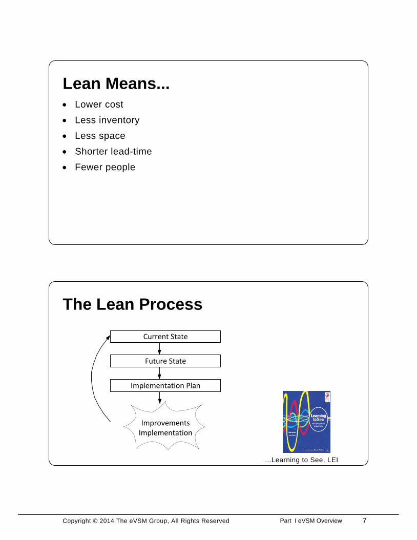
The Lean Process
Current State
Future State
Implementation Plan
Improvements Implementation
...Learning to See, LEI
Lean Means...· Lower cost
· Less inventory
· Less space
· Shorter lead-time
· Fewer people
7Part I eVSM Overview
Copyright © 2014 The eVSM Group, All Rights Reserved
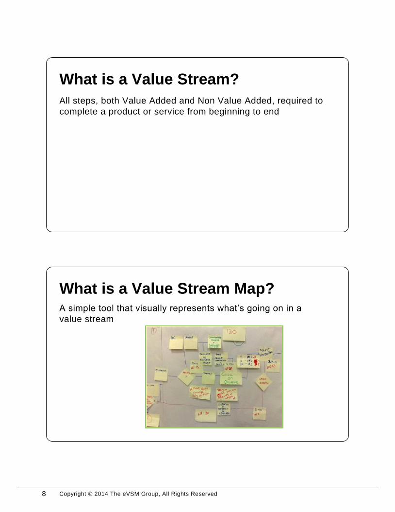
What is a Value Stream Map?A simple tool that visually represents what’s going on in a
value stream
What is a Value Stream?
All steps, both Value Added and Non Value Added, required to
complete a product or service from beginning to end
8
Copyright © 2014 The eVSM Group, All Rights Reserved
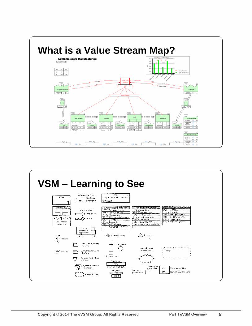
What is a Value Stream Map?ACME Scissors Manufacturing
Current State
Z020
Customer
7000Customer Daily Demand
Item
1
14
Day
Hr
60
Hr
Min
60
Min
Sec
1Activity Lead Time
Day
A010
ATLAS Warehouse
1
1.07 Day
Type
7500Inventory Item
A030 1
1Time
BetweenDay
A020 1
0.80 Min
1Associates Staff
10Qty Per Cycle Item
0.8Cycle Time Min
Mold Handles
A050 1
0.55 Day
Blanks
3850Inventory Item
A060 1
2.20 Min
1Associates Staff
10Qty Per Cycle Item
2.2Cycle Time Min
Sharpen
A070 1
0.39 Day
Sharp Blanks
2700Inventory Item
A080 1
0.50 Min
1Associates Staff
10Qty Per Cycle Item
0.5Cycle Time Min
A090 1
0.44 Day
Drilled Blanks
3100Inventory Item
A100 1
1.00 Min
1Associates Staff
10Qty Per Cycle Item
1Cycle Time Min
Assemble
A110 1
1.29 Day
Scissors
9000Inventory Item
A120 1
MRP
Production
Control
Forecast 30 Days
Weekly Order
Daily
Daily
Weekly Schedule
Z010
Time Summary 1
0.12Takt Time Min
4.50Total Value
AddedMin
6.74Lead Time Day
0.08Value Added
Percent%
1
Z140
Time Summary 2
0.12Takt Time Min
6.00Total Value
AddedMin
2.64Lead Time Day
0.27Value Added
Percent%
2
1Time
BetweenDay
A150 1
2
2Stations Stn8Activity Time
Per Day Hr 9000Activity Daily
DemandItem
Drill
2
2
2
Cycle Time / Takt Time Chart
Min
0
0.02
0.04
0.06
0.08
0.1
0.12
A050
Mold Han
dles
A070
Sharpe
n
A090
Drill
A110
Assem
ble
A160
Cardb
oard
Box
es
Cycle Time Per Item
Activity Takt Time
VSM – Learning to See
9Part I eVSM Overview
Copyright © 2014 The eVSM Group, All Rights Reserved
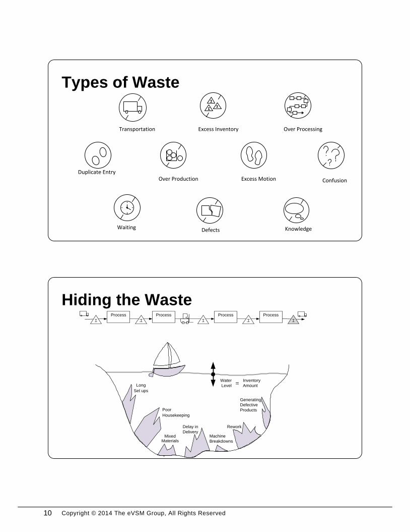
Types of Waste
Hiding the Waste
Generating
Defective
Products
Machine
Breakdowns
ReworkDelay in
DeliveryMixed
Materials
Poor
Housekeeping
Long
Set ups
Process Process Process Process
=Water
Level
Inventory
Amount
Excess Inventory
Excess MotionOver Production
Transportation
Waiting
Over Processing
Confusion
Duplicate Entry
Defects Knowledge
10
Copyright © 2014 The eVSM Group, All Rights Reserved
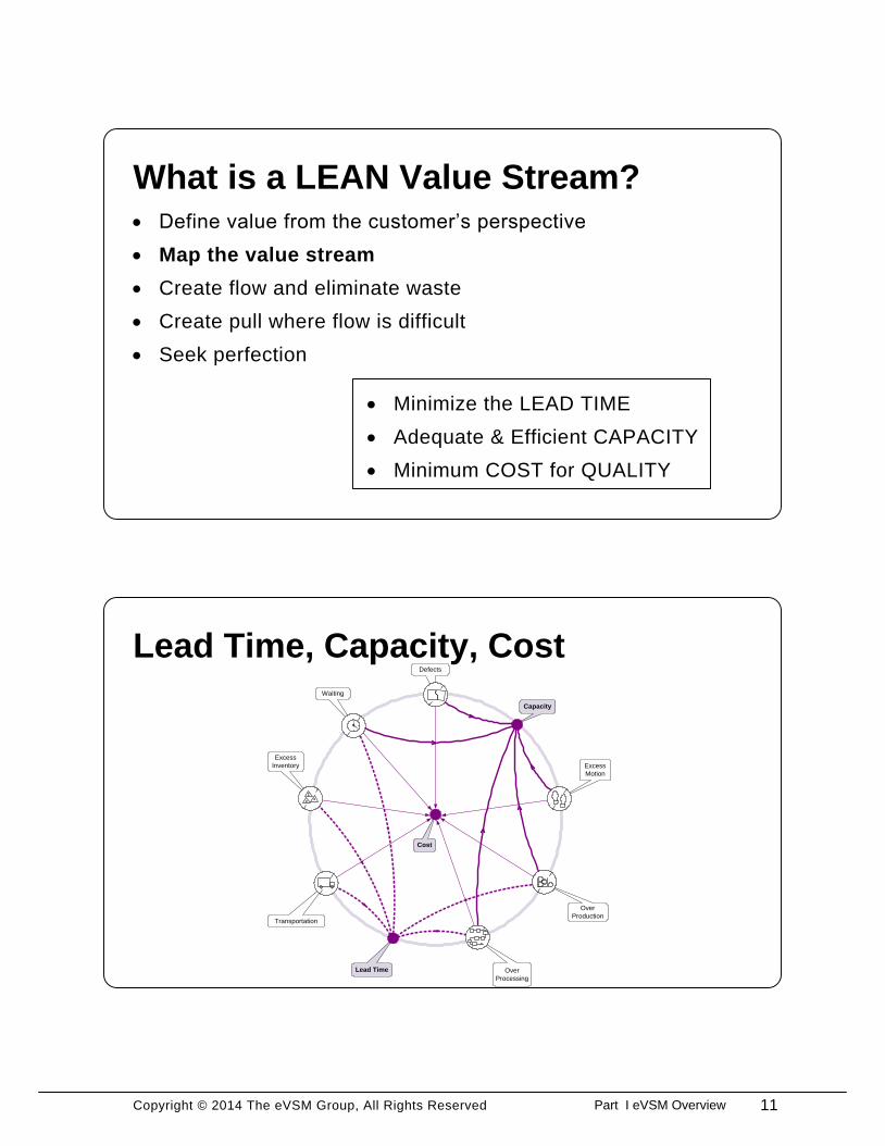
What is a LEAN Value Stream?· Define value from the customer’s perspective
· Map the value stream
· Create flow and eliminate waste
· Create pull where flow is difficult
· Seek perfection
· Minimize the LEAD TIME
· Adequate & Efficient CAPACITY
· Minimum COST for QUALITY
Lead Time, Capacity, Cost
Excess
Inventory
Waiting
Defects
Over
ProductionTransportation
Excess
Motion
Over
Processing
Capacity
Lead Time
Cost
11Part I eVSM Overview
Copyright © 2014 The eVSM Group, All Rights Reserved
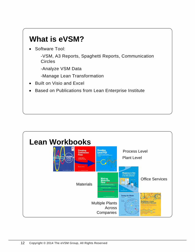
What is eVSM?· Software Tool:
-VSM, A3 Reports, Spaghetti Reports, Communication
Circles
-Analyze VSM Data
-Manage Lean Transformation
· Built on Visio and Excel
· Based on Publications from Lean Enterprise Institute
Lean WorkbooksProcess Level
Plant Level
Office Services
Multiple Plants
Across
Companies
Materials
12
Copyright © 2014 The eVSM Group, All Rights Reserved
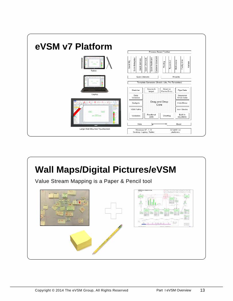
eVSM v7 Platform
Wall Maps/Digital Pictures/eVSMValue Stream Mapping is a Paper & Pencil tool
13Part I eVSM Overview
Copyright © 2014 The eVSM Group, All Rights Reserved
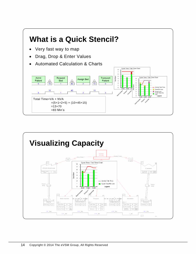
· Very fast way to map
· Drag, Drop & Enter Values
· Automated Calculation & Charts
What is a Quick Stencil?
Total Time=VA + NVA
=(5+1+2+5) + (10+45+15)
=13+70
=83 Min’s
Cycle Time / Takt Time Chart
Sec/I
tem
0
1
2
3
4
5
6
7
8
A040
Mol
d Han
dles
A060
Sha
rpen
A080
Ass
embl
e
Cycle Time Per Unit
Legend
Changeover Loss
Activity Takt Time
Cycle Time / Takt Time Chart
Sec/Ite
m
0
1
2
3
4
5
6
7
8
A040
Mold
Han
dles
A060
Sha
rpen
A080
Ass
emble
Cycle Time Per
UnitLegend
Scrap Loss
DownStr Loss
Activity Takt Time
Visualizing Capacity
14
Copyright © 2014 The eVSM Group, All Rights Reserved
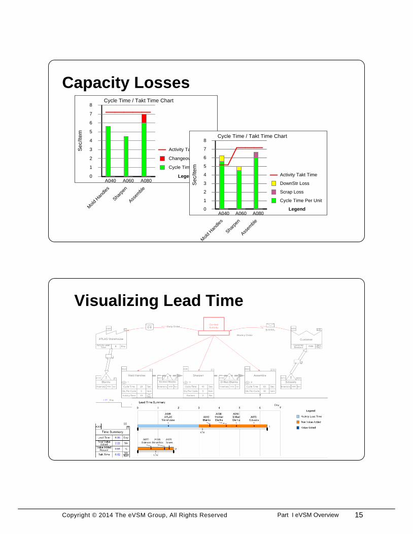
Capacity LossesCycle Time / Takt Time Chart
Sec/Ite
m
0
1
2
3
4
5
6
7
8
A040
Mold
Han
dles
A060
Sharp
en
A080
Ass
emble
Cycle Time Per Unit
Legend
Changeover Loss
Activity Takt Time
Cycle Time / Takt Time Chart
Sec/Ite
m
0
1
2
3
4
5
6
7
8
A040
Mold
Han
dles
A060
Sha
rpen
A080
Ass
emble
Cycle Time Per Unit
Legend
Scrap Loss
DownStr Loss
Activity Takt Time
Visualizing Lead Time
15Part I eVSM Overview
Copyright © 2014 The eVSM Group, All Rights Reserved
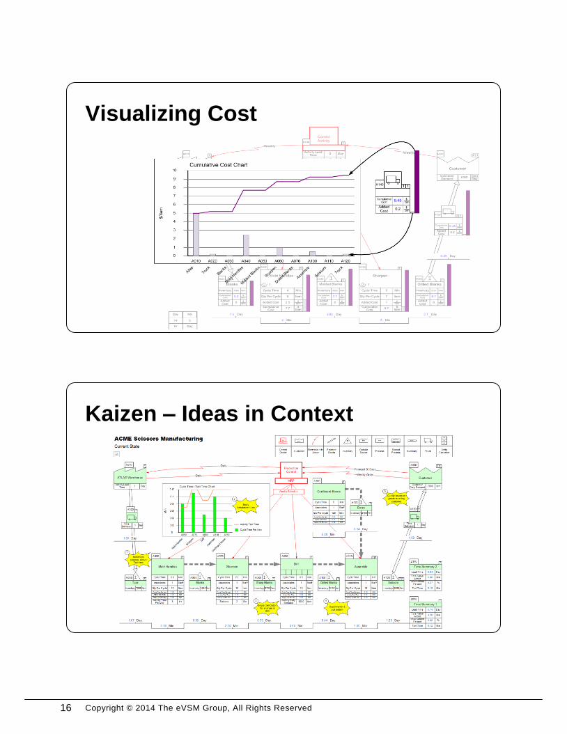
Visualizing Cost
Kaizen – Ideas in Context
16
Copyright © 2014 The eVSM Group, All Rights Reserved
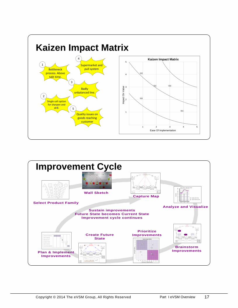
Kaizen Impact Matrix
Bottleneck process. Above
takt time.
1
Badly unbalanced line.
Single cell option for sharpen and
drill.
Supermarket and pull system
Quality issues on goods reaching
customer
2
3
4
5
Improvement Cycle
Cycle Time / Takt Time Chart
Sec/Ite
m
0
1
2
3
4
5
6
7
8
A040 A060 A080
Cycle Time Per Unit
Activity Takt Time
2
01
81
61
41
21
0
8
6
4
2
2 4 6 81
0
1
2
1
4
1
6
1
8
2
0
IV
I
II
III
Difficulty Of Implementation
Imp
act O
n V
alu
e
Kaizen Impact Matrix
1
2
3
4
14
Day
Hr
5
Wk
Day
all
Customer
Customer Demand
ItemDay
7000
A0101
ATLAS Warehouse
Activity Lead Time
Day0
A020
Control
Activity
1
Blanks
Day1.07
Inventory Item7500
A030
1
Mold Handles
Min0.47
Qty Per Cycle Item5
Cycle Time Sec28
1
A040
1
Molded Blanks
Day0.55
Inventory Item3850
A050
1
Sharpen
Min0.75
Qty Per Cycle Item5
Cycle Time Sec45
1
A060
1
Drilled Blanks
Day0.44
Inventory Item3100
A070
1
Assemble
Min1
Qty Per Cycle Item10
Cycle Time Sec60
2
A080
1
Scissors
Inventory Item9000
A090
Activity TimeHr
Day10 Stations Stn2
Daily Order Weekly Order
1
Day0.44
Time Summary
Takt TimeMinItem
0.12
Total Value Added
Min2.22
Lead Time Day2.07
Value Added Percent
%0.13
Z010
Lead Time Summary
Day
0 0.2 0.4 0.6 0.8 1 1.2 1.4 1.6 1.8 2 2.2
A030Blanks
A050Molded Blanks
A070Drilled Blanks
2.06
Non Value Added
Legend
Value Added
U-shape Layout for Assembly Cell
Replace D4 Drilling Station
Milling Inventory Area 5S
New lighting in Hanger 501
Replace D7 Drilling Station
Group Value Stream Mapping Event
Select Product Family
Wall SketchCapture Map
Analyze and Visualize
Brainstorm
Improvements
Prioritize
ImprovementsCreate Future
State
Plan & Implement
Improvements
Sustain improvements
Future State becomes Current State
Improvement cycle continues
5
4
3
2
1
1 2 3 4 5
Ease Of Implementation
Imp
act O
n V
alu
e
Kaizen Impact Matrix
001
002
003
004
005
17Part I eVSM Overview
Copyright © 2014 The eVSM Group, All Rights Reserved
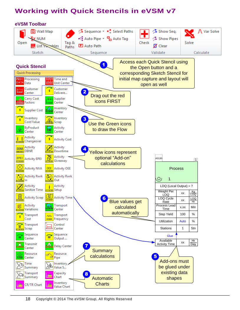
Working with Quick Stencils in eVSM v7
Quick Stencil
Add-ons must
be glued under
existing data
shapes
Drag out the red
icons FIRST
Use the Green icons
to draw the Flow
Yellow icons represent
optional “Add-on”
calculations
Glue
eVSM Toolbar
Access each Quick Stencil using
the Open button and a
corresponding Sketch Stencil for
initial map capture and layout will
open as well
Blue values get
calculated
automatically
Summary
calculations
Automatic
Charts
1
2
3
4
5
7
8
6
Process
A01301
1
LOQ (Local Output) = ?
Stations Stn1
Utilization %Auto
LOQ Cycle Rate
LOQHr
xx
Weight Per LOQ
KgLOQ
xx
Step Yield %100
Process Lead Time
Minx.xx
Available Activity Time
HrDay
xx
18
Copyright © 2014 The eVSM Group, All Rights Reserved
LOQ (Local Output) = ?
Stations Stn1
Utilization %Auto
LOQ Cycle Rate
LOQHr
xx
Weight Per LOQ
KgLOQ
xx
Step Yield %100
Process Lead Time
Minx.xx
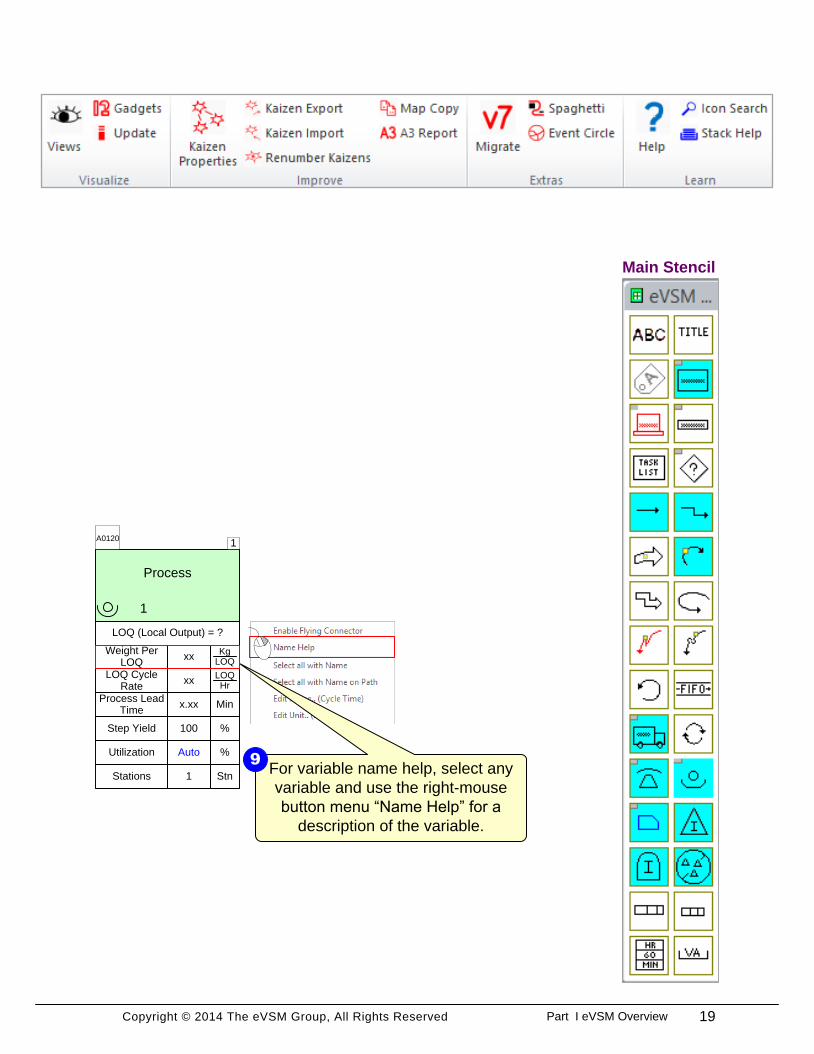
Main Stencil
For variable name help, select any
variable and use the right-mouse
button menu “Name Help” for a
description of the variable.
9
Process
A01201
1
19Part I eVSM Overview
Copyright © 2014 The eVSM Group, All Rights Reserved
Quick Stencil – Try This:
1. Go to a new page and use the “Open” command to access the Quick Processing stencil.
2. Which icons from the stencil must be put on the map first?
3. Drag out an Activity Center from the stencil. How do you get a quick description of a
variable in the center?
4. What is the meaning of the blue “Auto” value in the Activity Center?
20
Copyright © 2014 The eVSM Group, All Rights Reserved
Part II: Plant Level Mapping
21Part II Plant Level Mapping
Copyright © 2014 The eVSM Group, All Rights Reserved
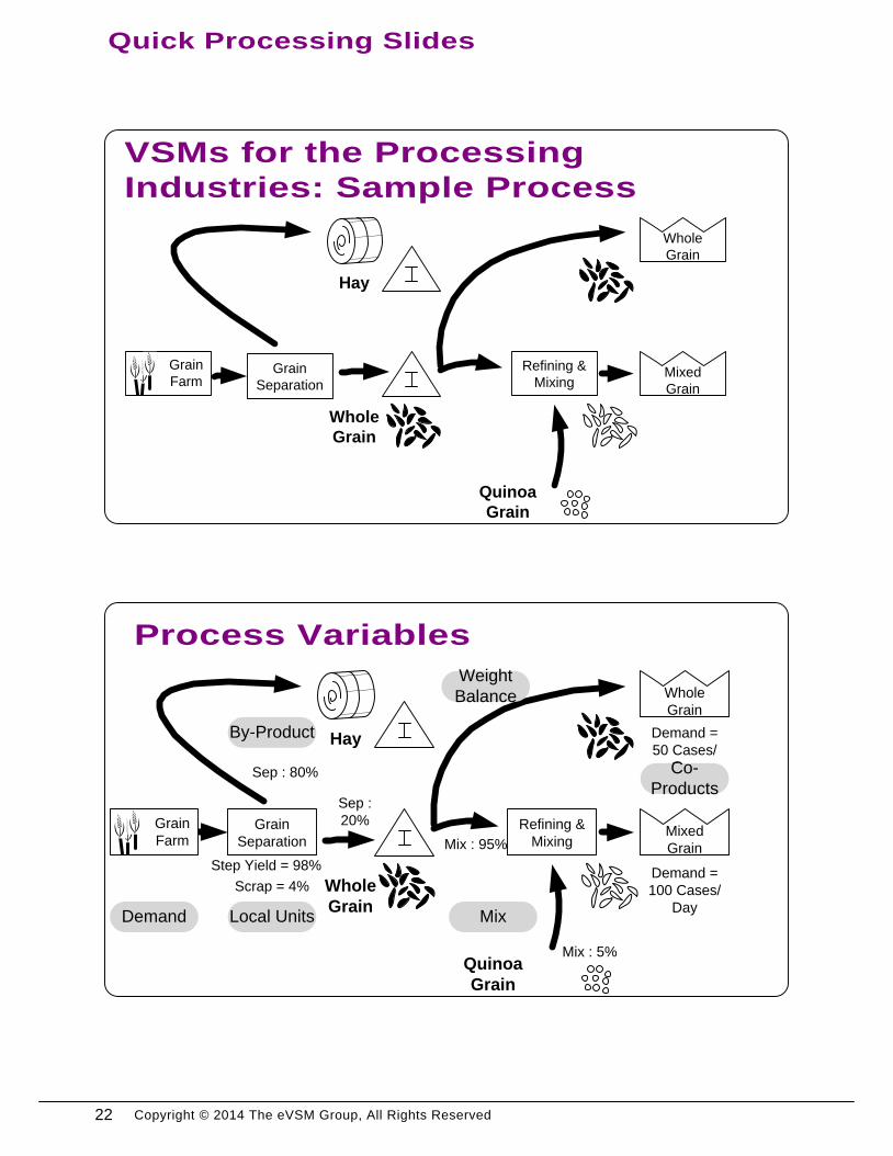
VSMs for the Processing
Industries: Sample Process
Grain
Separation
Refining &
Mixing
Hay
Whole
Grain
Quinoa
Grain
Grain
Farm
Whole
Grain
Mixed
Grain
Process Variables
Grain
Separation
Refining &
Mixing
Sep :
20%
Sep : 80%
Demand =
50 Cases/
Day
Hay
Whole
Grain
Demand =
100 Cases/
Day
Quinoa
Grain
Mix : 95%
Local Units Demand
By-Product
Co-
Products
Grain
Farm
Whole
Grain
Mixed
Grain
Mix : 5%
Mix
Step Yield = 98%
Scrap = 4%
Weight
Balance
Quick Processing Slides
22
Copyright © 2014 The eVSM Group, All Rights Reserved
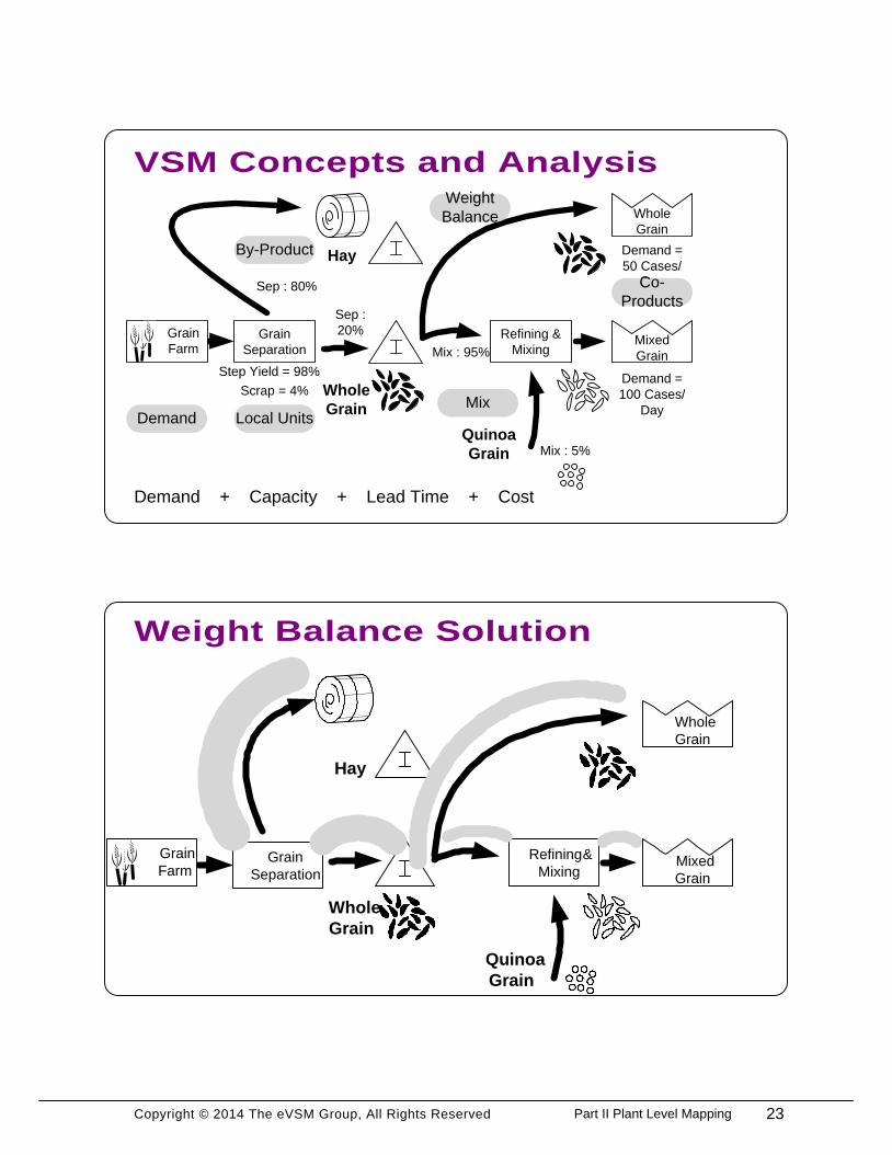
VSM Concepts and Analysis
Weight Balance Solution
Grain
Separation
Refining &
Mixing
Sep :
20%
Sep : 80%
Demand =
50 Cases/
Day
Hay
Whole
Grain
Demand =
100 Cases/
Day
Quinoa
Grain
Mix : 95%
Local Units Demand
By-Product
Co-
Products
Grain
Farm
Whole
Grain
Mixed
Grain
Mix : 5%
Mix
Step Yield = 98%
Scrap = 4%
Weight
Balance
Demand Capacity Lead Time Cost+ + +
Grain
Separation
Refining &
Mixing
Hay
Whole
Grain
Quinoa
Grain
Grain
Farm
Whole
Grain
Mixed
Grain
Demand + Capacity + Lead Time + Cost
23Part II Plant Level Mapping
Copyright © 2014 The eVSM Group, All Rights Reserved
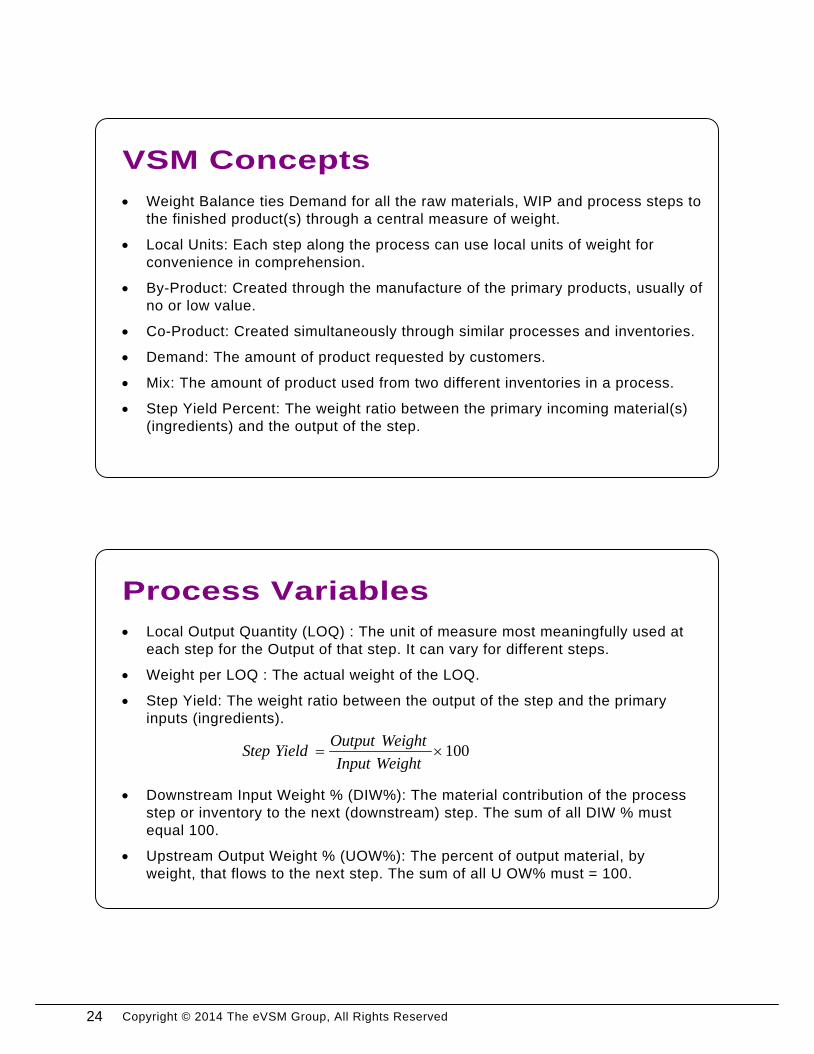
VSM Concepts
· Weight Balance ties Demand for all the raw materials, WIP and process steps to
the finished product(s) through a central measure of weight.
· Local Units: Each step along the process can use local units of weight for
convenience in comprehension.
· By-Product: Created through the manufacture of the primary products, usually of
no or low value.
· Co-Product: Created simultaneously through similar processes and inventories.
· Demand: The amount of product requested by customers.
· Mix: The amount of product used from two different inventories in a process.
· Step Yield Percent: The weight ratio between the primary incoming material(s)
(ingredients) and the output of the step.
Process Variables
100WeightInput
WeightOutputYieldStep
· Local Output Quantity (LOQ) : The unit of measure most meaningfully used at
each step for the Output of that step. It can vary for different steps.
· Weight per LOQ : The actual weight of the LOQ.
· Step Yield: The weight ratio between the output of the step and the primary
inputs (ingredients).
· Downstream Input Weight % (DIW%): The material contribution of the process
step or inventory to the next (downstream) step. The sum of all DIW % must
equal 100.
· Upstream Output Weight % (UOW%): The percent of output material, by
weight, that flows to the next step. The sum of all U OW% must = 100.
24
Copyright © 2014 The eVSM Group, All Rights Reserved
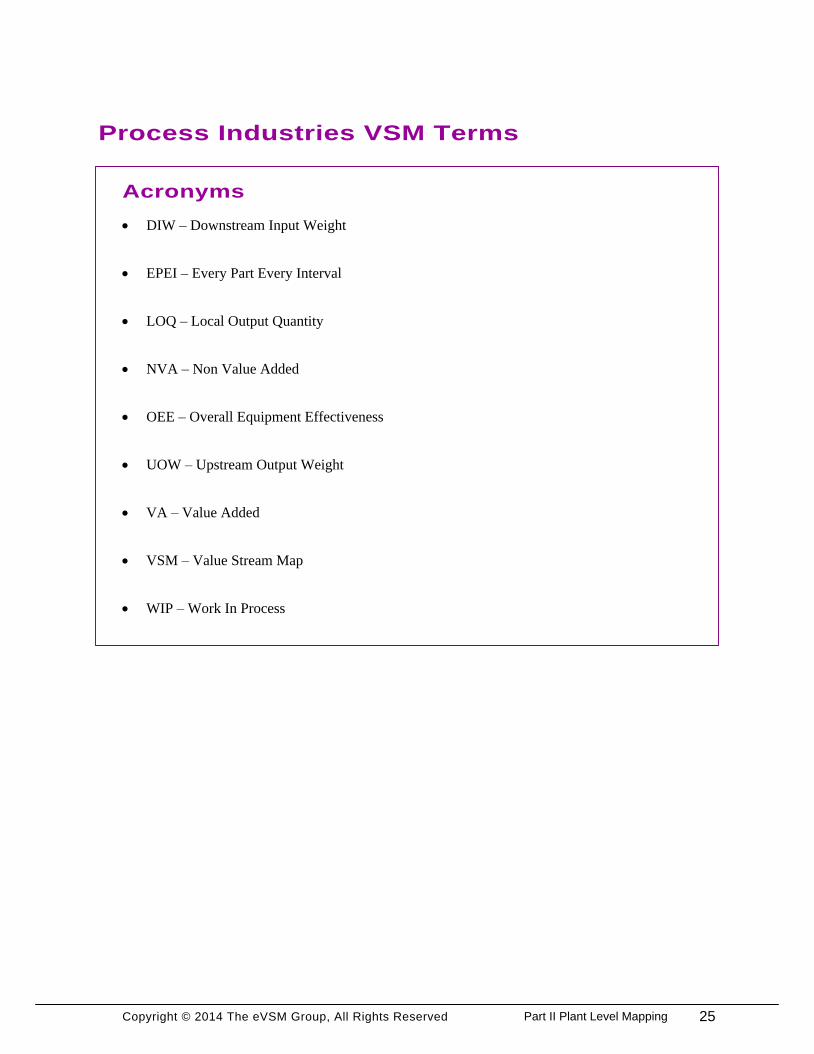
Process Industries VSM Terms
Acronyms
· LOQ – Local Output Quantity
· DIW – Downstream Input Weight
· UOW – Upstream Output Weight
· OEE – Overall Equipment Effectiveness
· NVA – Non Value Added
· VA – Value Added
· VSM – Value Stream Map
· EPEI – Every Part Every Interval
· WIP – Work In Process
25Part II Plant Level Mapping
Copyright © 2014 The eVSM Group, All Rights Reserved
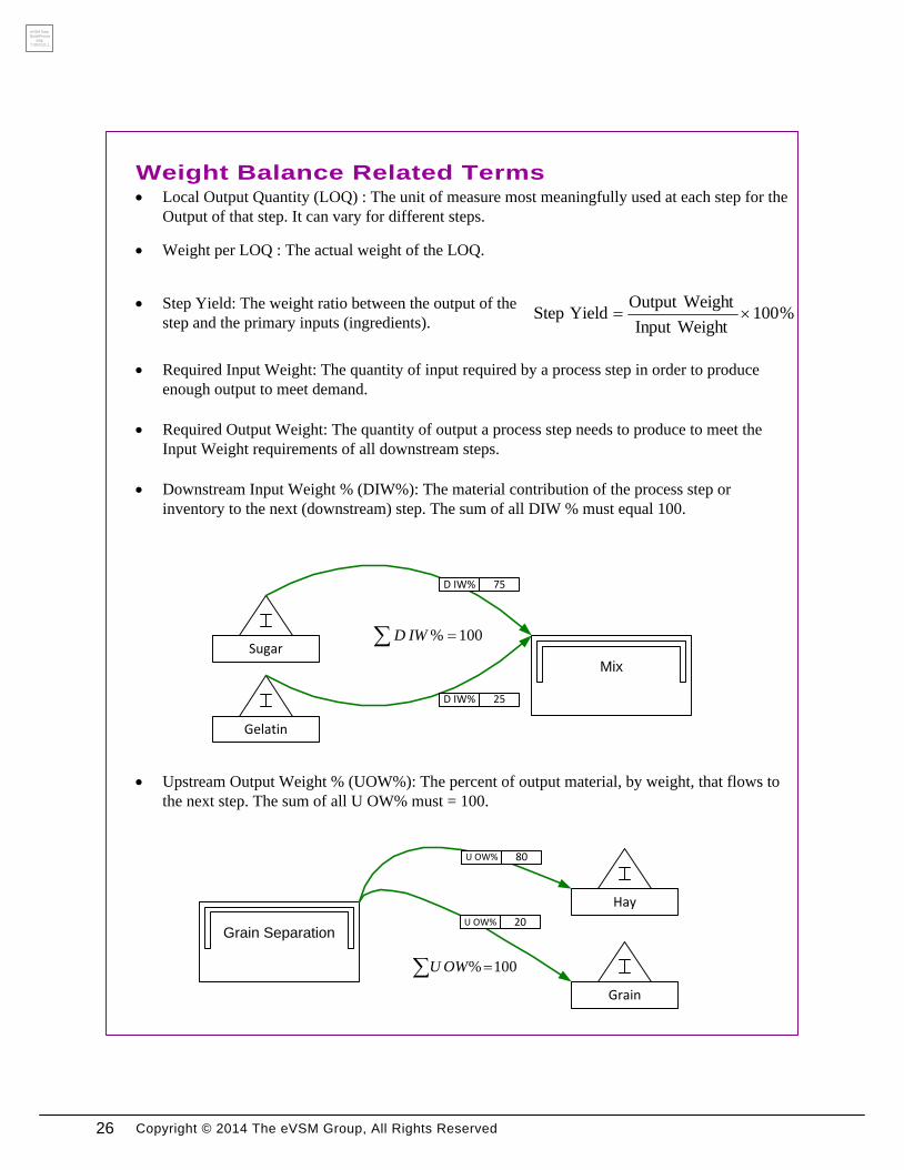
Weight Balance Related Terms
· Downstream Input Weight % (DIW%): The material contribution of the process step or
inventory to the next (downstream) step. The sum of all DIW % must equal 100.
SugarMix
Gelatin
D IW% 75
D IW% 25
· Step Yield: The weight ratio between the output of the
step and the primary inputs (ingredients). %100
WeightInput
WeightOutputYieldStep
100%IWD
· Upstream Output Weight % (UOW%): The percent of output material, by weight, that flows to
the next step. The sum of all U OW% must = 100.
Hay
Grain Separation
Grain
U OW% 80
U OW% 20
100%OWU
· Local Output Quantity (LOQ) : The unit of measure most meaningfully used at each step for the
Output of that step. It can vary for different steps.
· Weight per LOQ : The actual weight of the LOQ.
· Required Input Weight: The quantity of input required by a process step in order to produce
enough output to meet demand.
· Required Output Weight: The quantity of output a process step needs to produce to meet the
Input Weight requirements of all downstream steps.
eVSM Data
QuickProces
sing
7.30.0111.1
26
Copyright © 2014 The eVSM Group, All Rights Reserved
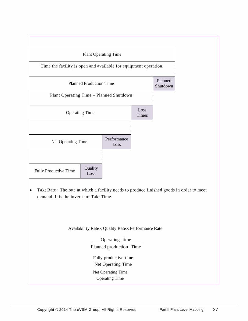
· Takt Rate : The rate at which a facility needs to produce finished goods in order to meet
demand. It is the inverse of Takt Time.
Plant Operating Time
Planned Production TimePlanned
Shutdown
Operating TimeLoss
Times
Net Operating TimePerformance
Loss
Fully Productive TimeQuality
Loss
Time the facility is open and available for equipment operation.
Plant Operating Time – Planned Shutdown
TimeproductionPlanned
timeOperating
RateePerformancRateQualityRatetyAvailabili
TimeOperatingNet
timeproductiveFully
TimeOperating
TimeOperatingNet
27Part II Plant Level Mapping
Copyright © 2014 The eVSM Group, All Rights Reserved
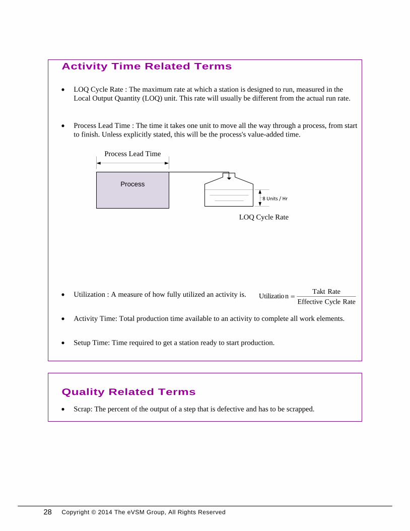
· LOQ Cycle Rate : The maximum rate at which a station is designed to run, measured in the
Local Output Quantity (LOQ) unit. This rate will usually be different from the actual run rate.
LOQ Cycle Rate
Process
8 Units / Hr
Process Lead Time
· Process Lead Time : The time it takes one unit to move all the way through a process, from start
to finish. Unless explicitly stated, this will be the process's value-added time.
· Utilization : A measure of how fully utilized an activity is.RateCycleEffective
RateTaktnUtilizatio
· Activity Time: Total production time available to an activity to complete all work elements.
· Setup Time: Time required to get a station ready to start production.
Activity Time Related Terms
Quality Related Terms
· Scrap: The percent of the output of a step that is defective and has to be scrapped.
28

Copyright © 2014 The eVSM Group, All Rights Reserved 29Part II Plant Level Mapping
Copyright © 2014 The eVSM Group, All Rights Reserved
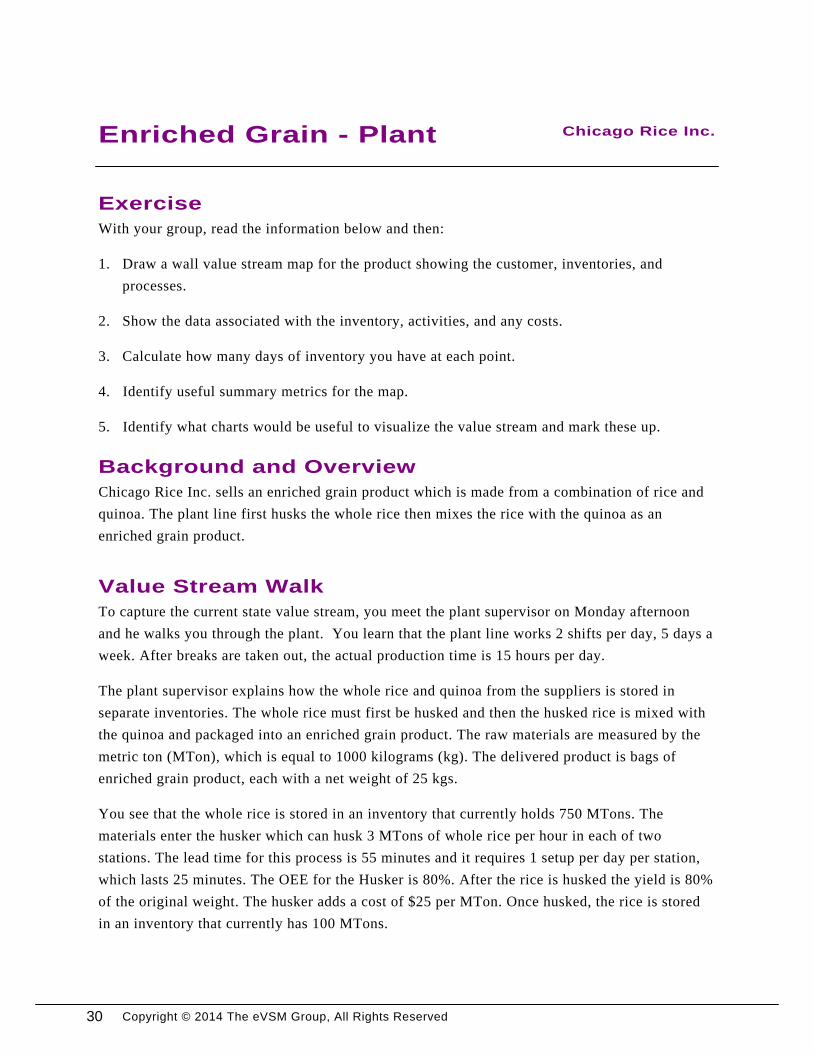
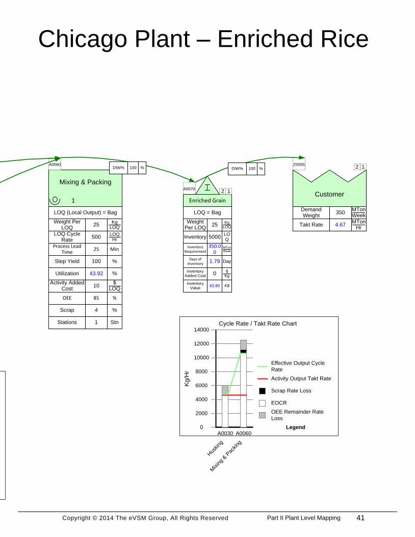
Enriched Grain - Plant Chicago Rice Inc.
Exercise
With your group, read the information below and then:
1. Draw a wall value stream map for the product showing the customer, inventories, and
processes.
2. Show the data associated with the inventory, activities, and any costs.
3. Calculate how many days of inventory you have at each point.
4. Identify useful summary metrics for the map.
5. Identify what charts would be useful to visualize the value stream and mark these up.
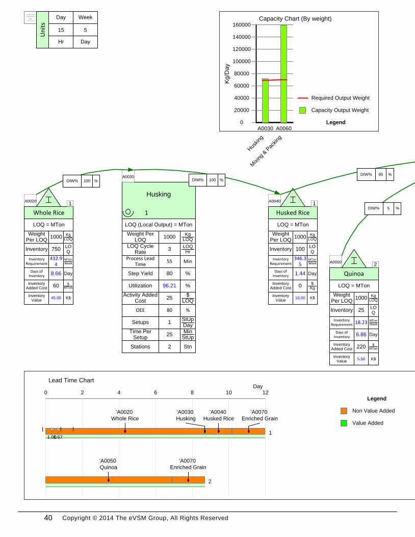
Background and Overview
Chicago Rice Inc. sells an enriched grain product which is made from a combination of rice and
quinoa. The plant line first husks the whole rice then mixes the rice with the quinoa as an
enriched grain product.
Value Stream Walk
To capture the current state value stream, you meet the plant supervisor on Monday afternoon
and he walks you through the plant. You learn that the plant line works 2 shifts per day, 5 days a
week. After breaks are taken out, the actual production time is 15 hours per day.
The plant supervisor explains how the whole rice and quinoa from the suppliers is stored in
separate inventories. The whole rice must first be husked and then the husked rice is mixed with
the quinoa and packaged into an enriched grain product. The raw materials are measured by the
metric ton (MTon), which is equal to 1000 kilograms (kg). The delivered product is bags of
enriched grain product, each with a net weight of 25 kgs.
You see that the whole rice is stored in an inventory that currently holds 750 MTons. The
materials enter the husker which can husk 3 MTons of whole rice per hour in each of two
stations. The lead time for this process is 55 minutes and it requires 1 setup per day per station,
which lasts 25 minutes. The OEE for the Husker is 80%. After the rice is husked the yield is 80%
of the original weight. The husker adds a cost of $25 per MTon. Once husked, the rice is stored
in an inventory that currently has 100 MTons.
30
Copyright © 2014 The eVSM Group, All Rights Reserved
Next, the quinoa is mixed and packed with the husked rice. The quinoa from the supplier is
stored in an inventory that currently holds 25 MTons. The rice and quinoa enter the mixing and
packing process which produces 500 bags of rice per hour. Each bag weighs 25 kgs and consists
of 95% husked rice and 5% quinoa. The lead time for this activity is 25 minutes and the yield is
100% of the original weight. The OEE of the mixing/packing process is 85%. The average
customer demand is 350 MTons/Week. There is scrap at this operation of 4% and the mixing
process costs an additional $10 per bag.
Once the enriched grain product is packed, it is stored in a finished goods inventory that
currently holds 5,000 bags.
31Part II Plant Level Mapping
Copyright © 2014 The eVSM Group, All Rights Reserved
eVSM Data
QuickProces
sing
7.30.0111.1
32
Copyright © 2014 The eVSM Group, All Rights Reserved
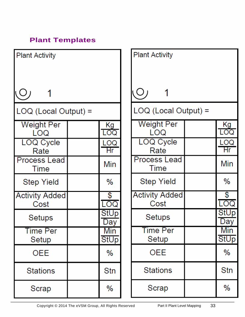
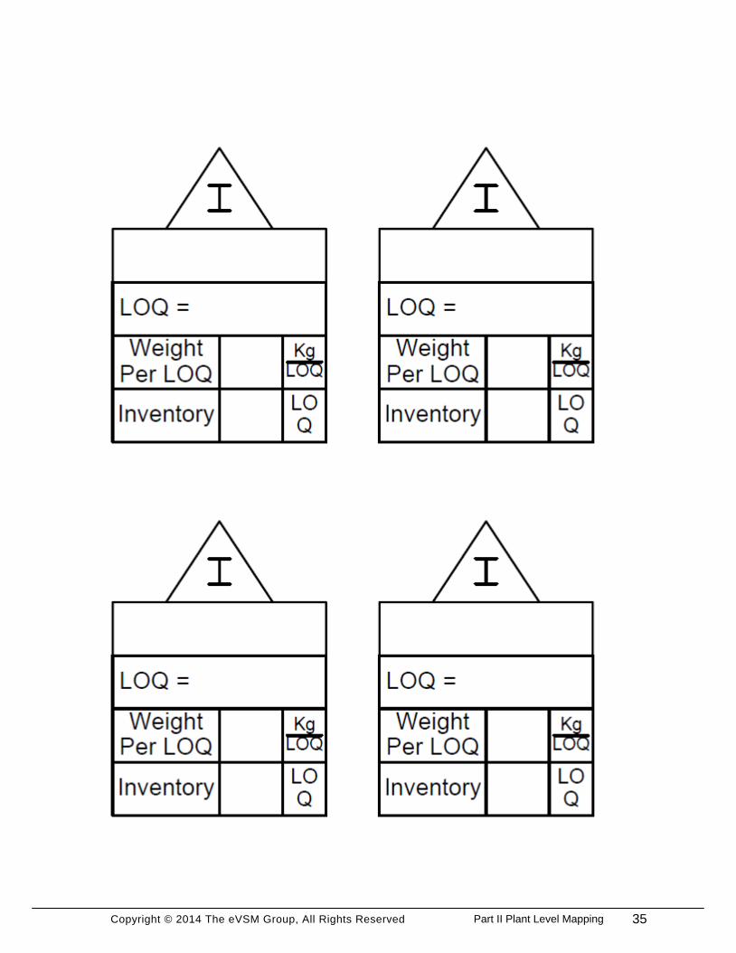
Plant Templates
33Part II Plant Level Mapping

Copyright © 2014 The eVSM Group, All Rights Reserved 34
Copyright © 2014 The eVSM Group, All Rights Reserved 35Part II Plant Level Mapping

Copyright © 2014 The eVSM Group, All Rights Reserved 36
Copyright © 2014 The eVSM Group, All Rights Reserved 37Part II Plant Level Mapping

Copyright © 2014 The eVSM Group, All Rights Reserved 38
Copyright © 2014 The eVSM Group, All Rights Reserved
eVSM Plant Workshop
1. Insert the picture of the wall map into eVSM using the Wall Map button in the toolbar. Refer
to the Sketcher section in the eVSM User Guide for help.
2. Use the Open command in the eVSM toolbar to open the Quick Processing stencil.
3. Draw the map in eVSM using the Quick Processing Stencil.
4. Create sequence arrows and note that the sum of the DIW values coming into an activity
needs to add up to 100%. Refer to the Sequence section of the eVSM User Guide for help.
5. Use the Auto Path button in the toolbar to assign path numbers. Refer to the AutoPath section
of the eVSM User Guide for help.
6. Use the Auto Tag button to sequentially number the tags. (this affects charting) Refer to the
AutoTag section of the eVSM User Guide for help.
7. Check the map and then Solve for the calculated fields.
8. Draw the Cycle Rate / Takt Rate chart to visualize capacity. Refer to the Charts section in the
eVSM User Guide for help.
9. Draw the Lead Time Chart.
10. Draw the Cumulative Cost Chart.
39Part II Plant Level Mapping
Copyright © 2014 The eVSM Group, All Rights Reserved
InventoryLOQ
750
LOQ = MTon
Weight Per LOQ
KgLOQ1000
A0020
Whole Rice
Days of Inventory
Day8.66
Husking
Utilization %96.21
1
LOQ (Local Output) = MTon
LOQ Cycle Rate
LOQHr
3
Weight Per LOQ
KgLOQ
1000
A0030
Step Yield %80
Process Lead Time
Min55
InventoryLOQ
100
LOQ = MTon
Weight Per LOQ
KgLOQ1000
A0040
Husked Rice
Days of Inventory
Day1.44
InventoryLOQ
25
LOQ = MTon
Weight Per LOQ
KgLOQ1000
A0050
Quinoa
Days of Inventory
Day6.86
Activity Added Cost
$LOQ
25
SetupsStUpDay
1
Time Per Setup
MinStUp
25
1
1
1
2
Capacity
Chart
Inventory Requirement
MTonWeek
432.94
Inventory Requirement
MTonWeek
346.35
Inventory Requirement
MTonWeek18.23
OEE %80
Stations Stn2
Inventory Added Cost
$Kg0
Inventory Value
K$10.00
Inventory Added Cost
$MTon60
Inventory Value
K$45.00
Inventory Added Cost
$MTon220
Inventory Value
K$5.50
DIW% %100 DIW% %100
DIW% %95
DIW% %5
Capacity Chart (By weight)
Kg
/Da
y
0
20000
40000
60000
80000
100000
120000
140000
160000
A0030
Hus
king
A0060
Mixing
& P
acking
Capacity Output Weight
Legend
Required Output Weight
Lead Time
Chart
all
Lead Time ChartDay
0 2 4 6 8 10 12
'A0020
Whole Rice
'A0030
Husking
'A0040
Husked Rice
'A0070
Enriched Grain
11.67
'A0050
Quinoa
'A0070
Enriched Grain
2
1.00
Non Value Added
Legend
Value Added
eVSM Data
QuickProces
sing
7.30.0111.1
5
Week
Day
15
Day
HrU
nit
s
40
Copyright © 2014 The eVSM Group, All Rights Reserved
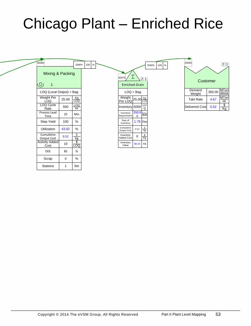
Takt RateMTon
Hr4.67
Customer
Z0005
Demand Weight
MTonWeek
350
Mixing & Packing
Utilization %43.92
1
LOQ (Local Output) = Bag
LOQ Cycle Rate
LOQHr
500
Weight Per LOQ
KgLOQ
25
A0060
Step Yield %100
Process Lead Time
Min25
InventoryLOQ
5000
LOQ = Bag
Weight Per LOQ
KgLOQ25
A0070
Enriched Grain
Days of Inventory
Day1.79
Activity Added Cost
$LOQ
10
Scrap %4
12
12
12
CR/TR
Chart
Chicago Plant – Enriched Rice
Inventory Requirement
MTonWeek
350.00
OEE %85
Inventory Added Cost
$Kg0
Inventory Value
K$63.80
Stations Stn1
DIW% %100 DIW% %100
Cycle Rate / Takt Rate Chart
Kg
/Hr
0
2000
4000
6000
8000
10000
12000
14000
A0030
Hus
king
A0060
Mixing
& P
acking
OEE Remainder Rate
Loss
Legend
EOCR
Scrap Rate Loss
Activity Output Takt Rate
Effective Output Cycle
Rate
Lead Time Chart
Non Value Added
Value Added
41Part II Plant Level Mapping

Copyright © 2014 The eVSM Group, All Rights Reserved 42
Copyright © 2014 The eVSM Group, All Rights Reserved
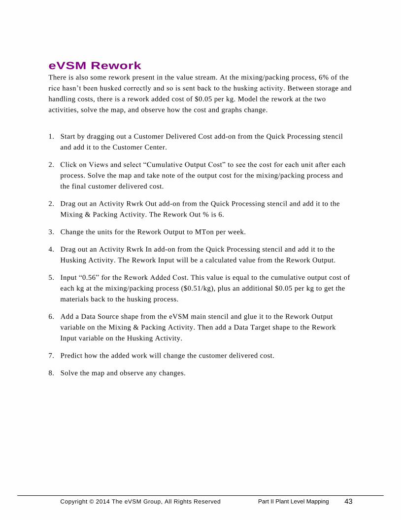
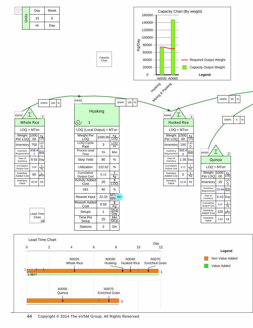
eVSM ReworkThere is also some rework present in the value stream. At the mixing/packing process, 6% of the
rice hasn’t been husked correctly and so is sent back to the husking activity. Between storage and
handling costs, there is a rework added cost of $0.05 per kg. Model the rework at the two
activities, solve the map, and observe how the cost and graphs change.
1. Start by dragging out a Customer Delivered Cost add-on from the Quick Processing stencil
and add it to the Customer Center.
2. Click on Views and select “Cumulative Output Cost” to see the cost for each unit after each
process. Solve the map and take note of the output cost for the mixing/packing process and
the final customer delivered cost.
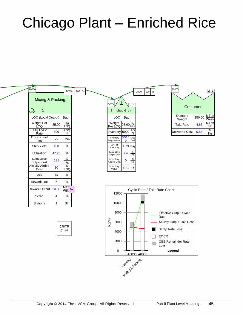
2. Drag out an Activity Rwrk Out add-on from the Quick Processing stencil and add it to the
Mixing & Packing Activity. The Rework Out % is 6.
3. Change the units for the Rework Output to MTon per week.
4. Drag out an Activity Rwrk In add-on from the Quick Processing stencil and add it to the
Husking Activity. The Rework Input will be a calculated value from the Rework Output.
5. Input “0.56” for the Rework Added Cost. This value is equal to the cumulative output cost of
each kg at the mixing/packing process ($0.51/kg), plus an additional $0.05 per kg to get the
materials back to the husking process.
6. Add a Data Source shape from the eVSM main stencil and glue it to the Rework Output
variable on the Mixing & Packing Activity. Then add a Data Target shape to the Rework
Input variable on the Husking Activity.
7. Predict how the added work will change the customer delivered cost.
8. Solve the map and observe any changes.
43Part II Plant Level Mapping
Copyright © 2014 The eVSM Group, All Rights Reserved
InventoryLOQ
750
LOQ = MTon
Weight Per LOQ
KgLOQ
1000.00
A0020
Whole Rice
Days of Inventory
Day8.55
Husking
Utilization %102.62
1
LOQ (Local Output) = MTon
LOQ Cycle Rate
LOQHr
3
Weight Per LOQ
KgLOQ
1000.00
A0030
Step Yield %80
Process Lead Time
Min55
InventoryLOQ
100
LOQ = MTon
Weight Per LOQ
KgLOQ
1000.00
A0040
Husked Rice
Days of Inventory
Day1.35
InventoryLOQ
25
LOQ = MTon
Weight Per LOQ
KgLOQ
1000.00
A0050
Quinoa
Days of Inventory
Day6.43
Activity Added Cost
$LOQ
25
SetupsStUpDay
1
Time Per Setup
MinStUp
25
1
1
1
2
Capacity
Chart
Inventory Requirement
MTonWeek
438.47
Inventory Requirement
MTonWeek
369.44
Inventory Requirement
MTonWeek19.44OEE %80
Stations Stn2
Inventory Added Cost
$Kg0
Inventory Value
K$13.16
Inventory Added Cost
$MTon60
Inventory Value
K$45.00
Inventory Added Cost
$MTon220
Inventory Value
K$5.50
Rework InputMTonWeek
23.33
Rework Added Cost
$Kg
0.56
RW
Cumulative Output Cost
$Kg
0.06
Cumulative Output Cost
$Kg
0.13
Cumulative Output Cost
$Kg
0.13
Cumulative Output Cost
$Kg
0.22
Lead Time
Chart
all
Capacity Chart (By weight)
Kg
/Da
y
0
20000
40000
60000
80000
100000
120000
140000
160000
A0030
Hus
king
A0060
Mixing
& P
acking
Capacity Output Weight
Legend
Required Output Weight
Lead Time ChartDay
0 2 4 6 8 10 12
'A0020
Whole Rice
'A0030
Husking
'A0040
Husked Rice
'A0070
Enriched Grain
11.67
'A0050
Quinoa
'A0070
Enriched Grain
2
1.00
Non Value Added
Legend
Value Added
DIW% %100 DIW% %100
DIW% %95
DIW% %5
eVSM Data
QuickProces
sing
7.30.0111.1
5
Week
Day
15
Day
HrU
nit
s
44
Copyright © 2014 The eVSM Group, All Rights Reserved
Takt RateMTon
Hr4.67
Customer
Z0005
Demand Weight
MTonWeek
350.00
Mixing & Packing
Utilization %47.26
1
LOQ (Local Output) = Bag
LOQ Cycle Rate
LOQHr
500
Weight Per LOQ
KgLOQ
25.00
A0060
Step Yield %100
Process Lead Time
Min25
InventoryLOQ
5000
LOQ = Bag
Weight Per LOQ
KgLOQ25.00
A0070
Enriched Grain
Days of Inventory
Day1.79
Activity Added Cost
$LOQ
10
Scrap %4
12
12
12
CR/TR
Chart
Chicago Plant – Enriched Rice
Inventory Requirement
MTonWeek
350.00
OEE %85
Inventory Added Cost
$Kg0
Inventory Value
K$67.71
Rework Out %6
Rework OutputMTonWeek
23.33 RW
Delivered Cost$
Kg0.54
Cumulative Output Cost
$Kg
0.54
Cumulative Output Cost
$Kg
0.54
Stations Stn1
Cycle Rate / Takt Rate Chart
Kg
/Hr
0
2000
4000
6000
8000
10000
12000
A0030
Hus
king
A0060
Mixing
& P
acking
OEE Remainder Rate
Loss
Legend
EOCR
Scrap Rate Loss
Activity Output Takt Rate
Effective Output Cycle
Rate
DIW% %100 DIW% %100
45Part II Plant Level Mapping

Copyright © 2014 The eVSM Group, All Rights Reserved 46
Copyright © 2014 The eVSM Group, All Rights Reserved
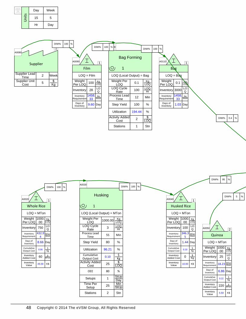
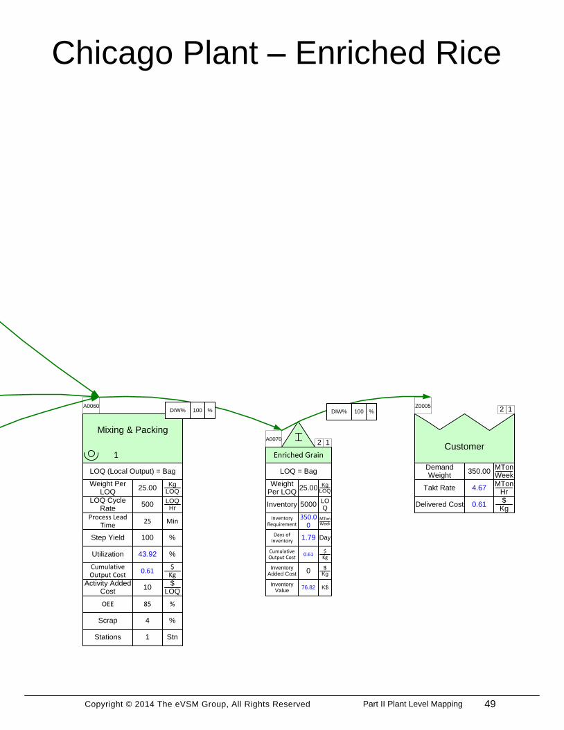
eVSM PackagingLets model the packaging activities explicitly on the map. The process starts from the supplier to
when the product is placed in the packaging. Raw material from the supplier costs $5/kg and
Added Activity Cost for forming the bag costs $2/bag. Each bag weighs 100 gm. Model the
packaging activities, solve the map, and observe how the delivered cost changes.
1. Start by drawing out the packaging value stream above the product value stream, this will
include the supplier, inventories and activities.
2. Sequence the new centers, with the final sequence connecting the Bag inventory to the
Mixing & Packing activity of the product VSM.
3. Each empty bag weighs 100 gm and holds 25 kg of product. So each bag is (100/25000 *
100) 0.4 % of the weight of the product. This is the value we will input for the DIW % on the
sequence arrow connecting the Bag inventory to the Mixing & Packing activity.
4. Add Supplier Cost and Activity Cost add-ons to the appropriate centers. Enter $5 for the
Supplier Unit Cost and $2 for the Activity Added Cost.
5. Predict how the packaging will change the customer delivered cost.
6. Solve the map and observe any changes.
47Part II Plant Level Mapping
Copyright © 2014 The eVSM Group, All Rights Reserved
InventoryLOQ
750
LOQ = MTon
Weight Per LOQ
KgLOQ
1000.00
A0020
Whole Rice
Days of Inventory
Day8.66
Husking
Utilization %96.21
1
LOQ (Local Output) = MTon
LOQ Cycle Rate
LOQHr
3
Weight Per LOQ
KgLOQ
1000.00
A0030
Step Yield %80
Process Lead Time
Min55
InventoryLOQ
100
LOQ = MTon
Weight Per LOQ
KgLOQ
1000.00
A0040
Husked Rice
Days of Inventory
Day1.44
InventoryLOQ
25
LOQ = MTon
Weight Per LOQ
KgLOQ
1000.00
A0050
Quinoa
Days of Inventory
Day6.86
Activity Added Cost
$LOQ
25
SetupsStUpDay
1
Time Per Setup
MinStUp
25
1
1
1
2
Inventory Requirement
MTonWeek
432.94
Inventory Requirement
MTonWeek
346.35
Inventory Requirement
MTonWeek18.23
OEE %80
Stations Stn2
Inventory Added Cost
$Kg0
Inventory Value
K$10.00
Inventory Added Cost
$MTon60
Inventory Value
K$45.00
Inventory Added Cost
$MTon220
Inventory Value
K$5.50
Cumulative Output Cost
$Kg
0.06
Cumulative Output Cost
$Kg
0.10
Cumulative Output Cost
$Kg
0.10
Cumulative Output Cost
$Kg
0.22
Supplier
A0080
1
Supplier Lead Time
Week2
Film
A00901
LOQ = Film
InventoryLOQ
28
Weight Per LOQ
KgLOQ100
Inventory Requirement
KgWeek
1458.33
Days of Inventory
Day9.60
Bag Forming
A01001
1
LOQ (Local Output) = Bag
Utilization %194.44
LOQ Cycle Rate
LOQHr
100
Weight Per LOQ
KgLOQ
0.1
Step Yield %100
Process Lead Time
Min12
Bag
A01101
LOQ = Bag
InventoryLOQ
3000
Weight Per LOQ
KgLOQ0.1
Inventory Requirement
KgWeek
1458.33
Days of Inventory
Day1.03
Supplier Unit Cost
$Kg
5
DIW% %100
DIW% %100DIW% %100
Activity Added Cost
$LOQ
2 DIW% %0.4
Stations Stn1
DIW% %100 DIW% %100
DIW% %95
DIW% %5
eVSM Data
QuickProces
sing
7.30.0111.1
5
Week
Day
15
Day
HrU
nit
s
48
Copyright © 2014 The eVSM Group, All Rights Reserved
Takt RateMTon
Hr4.67
Customer
Z0005
Demand Weight
MTonWeek
350.00
Mixing & Packing
Utilization %43.92
1
LOQ (Local Output) = Bag
LOQ Cycle Rate
LOQHr
500
Weight Per LOQ
KgLOQ
25.00
A0060
Step Yield %100
Process Lead Time
Min25
InventoryLOQ
5000
LOQ = Bag
Weight Per LOQ
KgLOQ25.00
A0070
Enriched Grain
Days of Inventory
Day1.79
Activity Added Cost
$LOQ
10
Scrap %4
12
12
12
Chicago Plant – Enriched Rice
Inventory Requirement
MTonWeek
350.00
OEE %85
Inventory Added Cost
$Kg0
Inventory Value
K$76.82
Delivered Cost$
Kg0.61
Cumulative Output Cost
$Kg
0.61
Cumulative Output Cost
$Kg
0.61
Stations Stn1
DIW% %100 DIW% %100
49Part II Plant Level Mapping

Copyright © 2014 The eVSM Group, All Rights Reserved 50
Copyright © 2014 The eVSM Group, All Rights Reserved
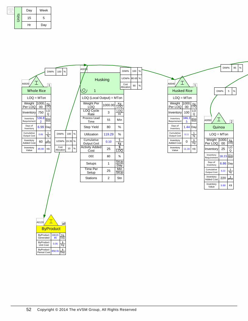
eVSM ByProductThe process of producing the enriched rice also produces a byproduct, husks, which can be used
in the process to make animal feed (a separate value stream). For every metric ton of rice
produced, 240 kg of husks is also produced. You decide to allocate 90% of the costs for
production (up through the Husking activity) to the rice and 10% to the husks. The allocation is
based on the relative value of the rice versus the husk. Find out how much husk is produced per
day, and what its value is.
1. Start by dragging out a ByProduct Center from the Quick Processing stencil, and placing it
below the Husking activity.
2. Add a sequence arrow from Husking to the ByProduct Center.
3. Now add a Sequence Output Weight add-on to the Sequence Center arrow, by gluing it to the
bottom of the DIW% data block. Also add the add-on to the Sequence Center arrow
connecting Husking to the Husked Rice inventory.
4. Since 120 kg of husk is produced for every 1000 kg of rice produced, it represents 19.35%
(240/(240+1000) * 100) and 80.65% (1000/(240+1000) * 100) of the total output of the
husking activity. Use these values for the respective UOW% (Upstream Output Weight %)
data blocks on the sequence arrows.
5. For the Cost Allocation from Husking to the ByProduct, use 10%, and 90% for Husking to
Husked Rice.
6. Solve the map and see how much husk is produced in a day and its value.
51Part II Plant Level Mapping
Copyright © 2014 The eVSM Group, All Rights Reserved
InventoryLOQ
750
LOQ = MTon
Weight Per LOQ
KgLOQ
1000.00
A0020
Whole Rice
Days of Inventory
Day6.99
Husking
Utilization %119.29
1
LOQ (Local Output) = MTon
LOQ Cycle Rate
LOQHr
3
Weight Per LOQ
KgLOQ
1000.00
A0030
Step Yield %80
Process Lead Time
Min55
InventoryLOQ
100
LOQ = MTon
Weight Per LOQ
KgLOQ
1000.00
A0040
Husked Rice
Days of Inventory
Day1.44
InventoryLOQ
25
LOQ = MTon
Weight Per LOQ
KgLOQ
1000.00
A0050
Quinoa
Days of Inventory
Day6.86
Activity Added Cost
$LOQ
25
SetupsStUpDay
1
Time Per Setup
MinStUp
25
1
1
1
2Inventory
RequirementMTonWeek
536.82
Inventory Requirement
MTonWeek
346.35
Inventory Requirement
MTonWeek18.23OEE %80
Stations Stn2
Inventory Added Cost
$Kg0
Inventory Value
K$11.16
Inventory Added Cost
$MTon60
Inventory Value
K$45.00
Inventory Added Cost
$MTon220
Inventory Value
K$5.50
Cumulative Output Cost
$Kg
0.06
Cumulative Output Cost
$Kg
0.10
Cumulative Output Cost
$Kg
0.11
Cumulative Output Cost
$Kg
0.22
ByProduct
A0120all
ByProduct Generated
KgDay
16619.85
ByProduct Unit Cost
$Kg
0.05
ByProduct Period Cost
$Day
858.91
DIW% %100 DIW% %100
DIW% %95
DIW% %5
DIW% %100
UOW% %19.35
Cost Allocation
%10
UOW% %80.65
Cost Allocation
%90
eVSM Data
QuickProces
sing
7.30.0111.1
5
Week
Day
15
Day
Hr
Un
its
52
Copyright © 2014 The eVSM Group, All Rights Reserved
Takt RateMTon
Hr4.67
Customer
Z0005
Demand Weight
MTonWeek
350.00
Mixing & Packing
Utilization %43.92
1
LOQ (Local Output) = Bag
LOQ Cycle Rate
LOQHr
500
Weight Per LOQ
KgLOQ
25.00
A0060
Step Yield %100
Process Lead Time
Min25
InventoryLOQ
5000
LOQ = Bag
Weight Per LOQ
KgLOQ25.00
A0070
Enriched Grain
Days of Inventory
Day1.79
Activity Added Cost
$LOQ
10
Scrap %4
12
12
12
Chicago Plant – Enriched Rice
Inventory Requirement
MTonWeek
350.00
OEE %85
Inventory Added Cost
$Kg0
Inventory Value
K$65.24
Delivered Cost$
Kg0.52
Cumulative Output Cost
$Kg
0.52
Cumulative Output Cost
$Kg
0.52
Stations Stn1
DIW% %100DIW% %100
53Part II Plant Level Mapping

Copyright © 2014 The eVSM Group, All Rights Reserved 54
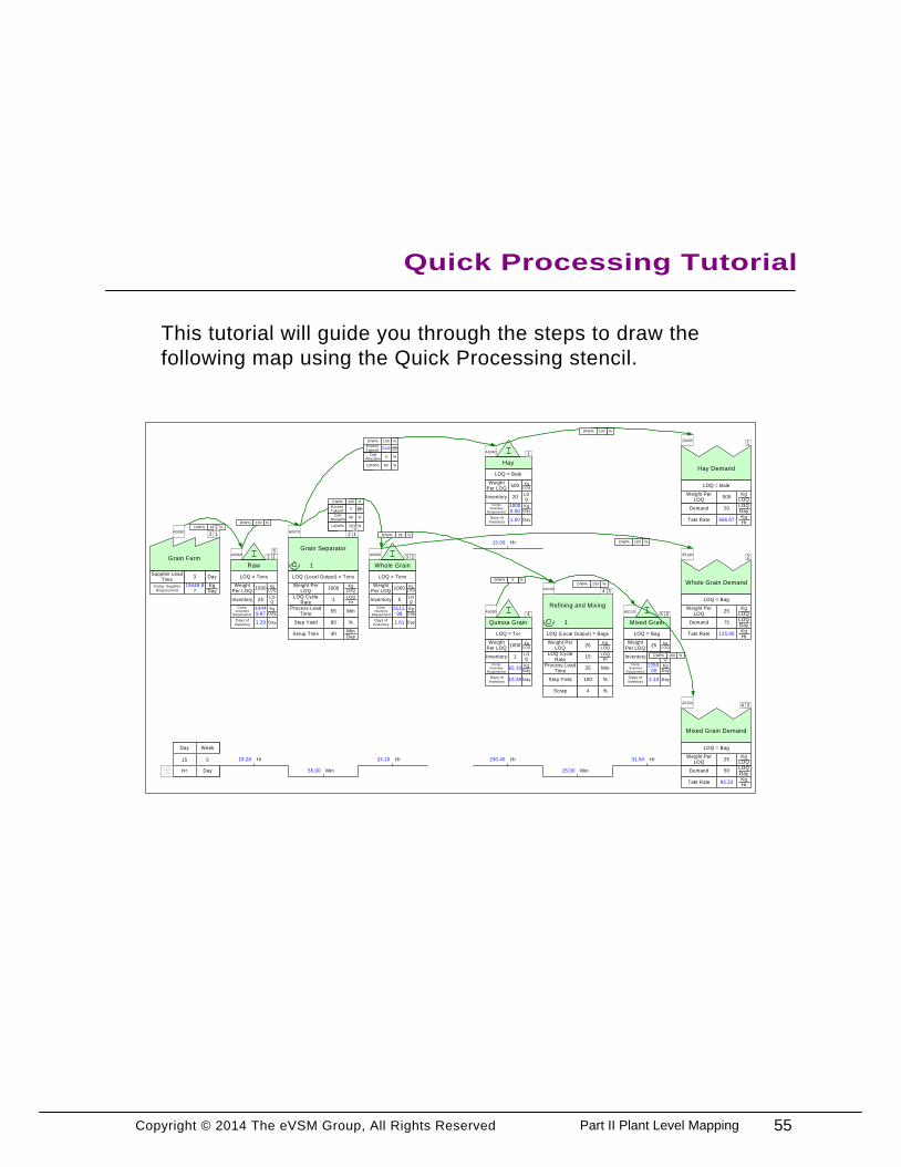
Copyright © 2014 The eVSM Group, All Rights Reserved
This tutorial will guide you through the steps to draw the
following map using the Quick Processing stencil.
Quick Processing Tutorial
Hr31.5015
Day
Hr
5
Week
Day
Takt RateKgHr
666.67
Hay Demand
DemandLOQDay
20
Weight Per LOQ
KgLOQ
500
LOQ = Bale
Z0005
Takt RateKgHr
125.00
Whole Grain Demand
DemandLOQDay
75
Weight Per LOQ
KgLOQ
25
LOQ = Bag
Z0140
Takt RateKgHr
83.33
Mixed Grain Demand
DemandLOQDay
50
Weight Per LOQ
KgLOQ
25
LOQ = Bag
Z0150
InventoryLOQ
20
LOQ = Bale
Weight Per LOQ
KgLOQ500
A0040
Hay
Hr15.00
Comp. Inventory
Requirement
KgDay
10000.00
Days of Inventory
Day1.00
Grain Farm
A0050
Supplier Lead Time
Day3
Comp. Supplier Requirement
KgDay
19449.87
InventoryLOQ
25
LOQ = Tons
Weight Per LOQ
KgLOQ1000
A0060
Raw
Hr19.28
Comp. Inventory
Requirement
KgDay
19449.87
Days of Inventory
Day1.29
Grain Separator
1
C
LOQ (Local Output) = Tons
LOQ Cycle Rate
LOQHr
1
Weight Per LOQ
KgLOQ
1000
A0070
Step Yield %80
Min55.00
Whole Grain
Process Lead Time
Min55
InventoryLOQ
5
LOQ = Tons
Weight Per LOQ
KgLOQ1000
A0080
Hr24.10
Comp. Inventory
Requirement
KgDay
3111.98
Days of Inventory
Day1.61
InventoryLOQ
1
LOQ = Tor
Weight Per LOQ
KgLOQ1000
A0090
Quinoa Grain
Hr230.40
Comp. Inventory
Requirement
KgDay
65.10
Days of Inventory
Day15.36
Refining and Mixing
1
LOQ (Local Output) = Bags
LOQ Cycle Rate
LOQHr
15
Weight Per LOQ
KgLOQ
25
A0100
Step Yield %100
Min25.00
Process Lead Time
Min25
InventoryLOQ
105
LOQ = Bag
Weight Per LOQ
KgLOQ25
A0110
Mixed Grain
Comp. Inventory
Requirement
KgDay
1250.00
Days of Inventory
Day2.10
eVSM Data
QuickProces
sing
6.23.0051.2
DIW% %100
DIW% %100
DIW% %100
DIW% %100
DIW% %100
DIW% %95
DIW% %100
DIW% %100
DIW% %100
DIW% %5
UOW% %80
Excess Takeoff
KgDay2448
Cost Allocation
%4
UOW% %20
Excess Takeoff
KgDay0
Cost Allocation
%96
1
1
1
1
1
2
2
2
2 2
3
3
3
3
3
3
3
4
4
4
4
Setup TimeMinDay
40
Scrap %4
55Part II Plant Level Mapping
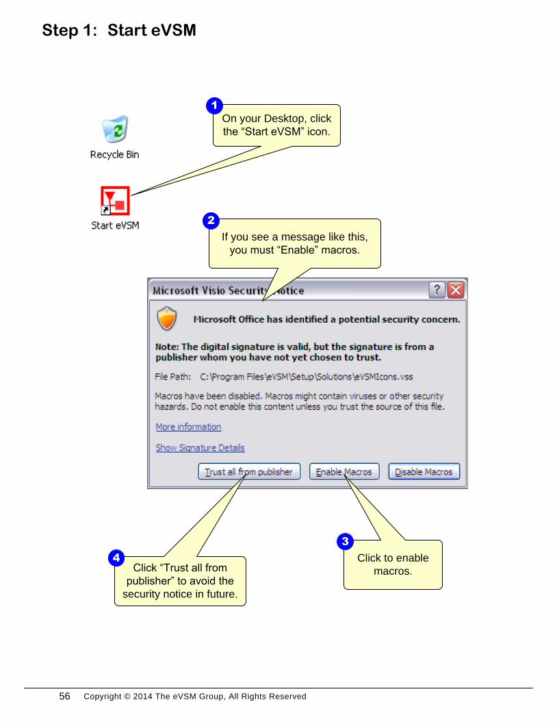
Copyright © 2014 The eVSM Group, All Rights Reserved
On your Desktop, click
the “Start eVSM” icon.
1
Click to enable
macros.Click “Trust all from
publisher” to avoid the
security notice in future.
3
4
If you see a message like this,
you must “Enable” macros.
2
Start eVSMStep 1:
56

Copyright © 2014 The eVSM Group, All Rights Reserved 57Part II Plant Level Mapping
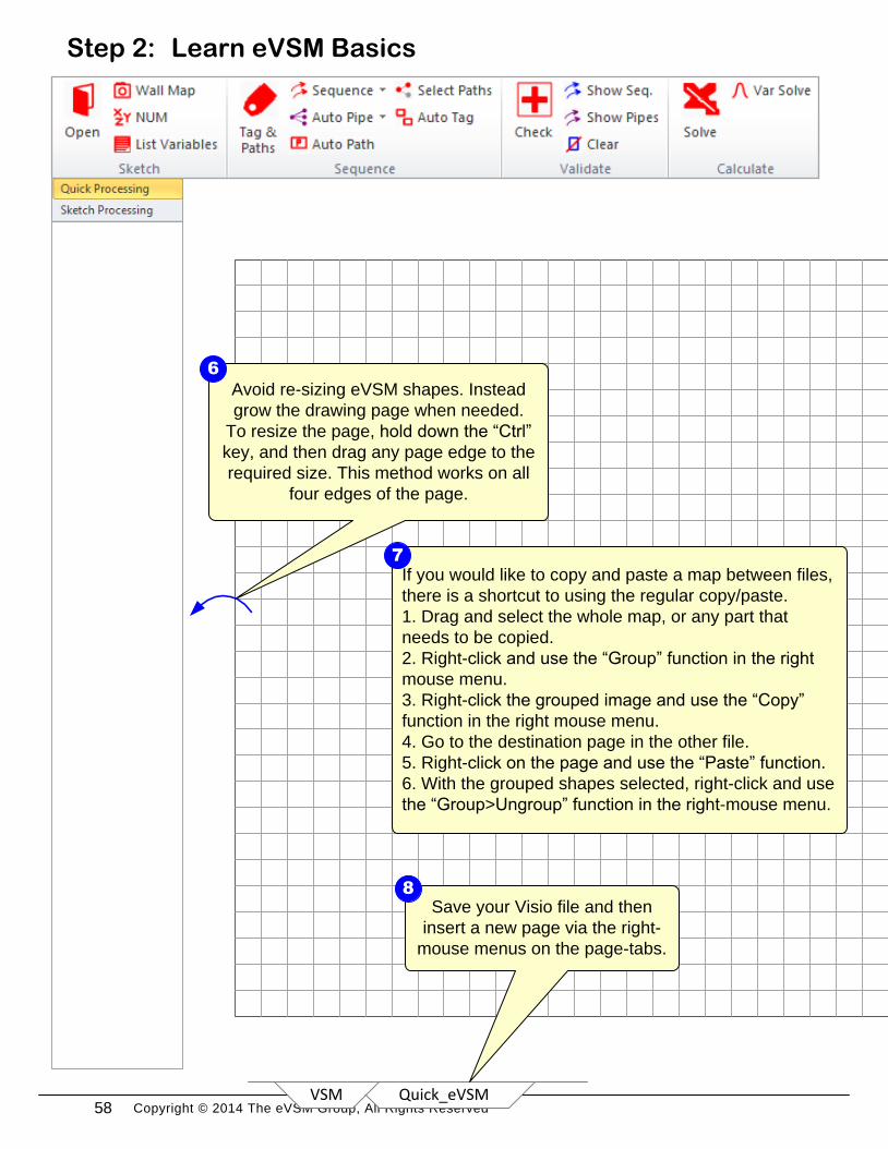
Copyright © 2014 The eVSM Group, All Rights Reserved Quick_eVSM
Learn eVSM BasicsStep 2:
Avoid re-sizing eVSM shapes. Instead
grow the drawing page when needed.
To resize the page, hold down the “Ctrl”
key, and then drag any page edge to the
required size. This method works on all
four edges of the page.
6
VSM
Save your Visio file and then
insert a new page via the right-
mouse menus on the page-tabs.
8
If you would like to copy and paste a map between files,
there is a shortcut to using the regular copy/paste.
1. Drag and select the whole map, or any part that
needs to be copied.
2. Right-click and use the “Group” function in the right
mouse menu.
3. Right-click the grouped image and use the “Copy”
function in the right mouse menu.
4. Go to the destination page in the other file.
5. Right-click on the page and use the “Paste” function.
6. With the grouped shapes selected, right-click and use
the “Group>Ungroup” function in the right-mouse menu.
7
58
Copyright © 2014 The eVSM Group, All Rights Reserved
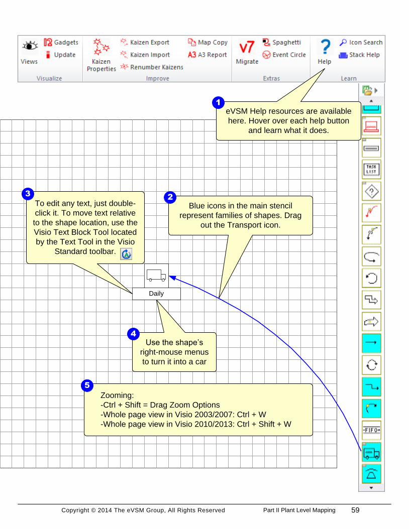
Learn eVSM Basics
eVSM Help resources are available
here. Hover over each help button
and learn what it does.
1
Blue icons in the main stencil
represent families of shapes. Drag
out the Transport icon.
Daily
2
Use the shape’s
right-mouse menus
to turn it into a car
4
Zooming:
-Ctrl + Shift = Drag Zoom Options
-Whole page view in Visio 2003/2007: Ctrl + W
-Whole page view in Visio 2010/2013: Ctrl + Shift + W
5
To edit any text, just double-
click it. To move text relative
to the shape location, use the
Visio Text Block Tool located
by the Text Tool in the Visio
Standard toolbar.
3
59Part II Plant Level Mapping
Copyright © 2014 The eVSM Group, All Rights Reserved
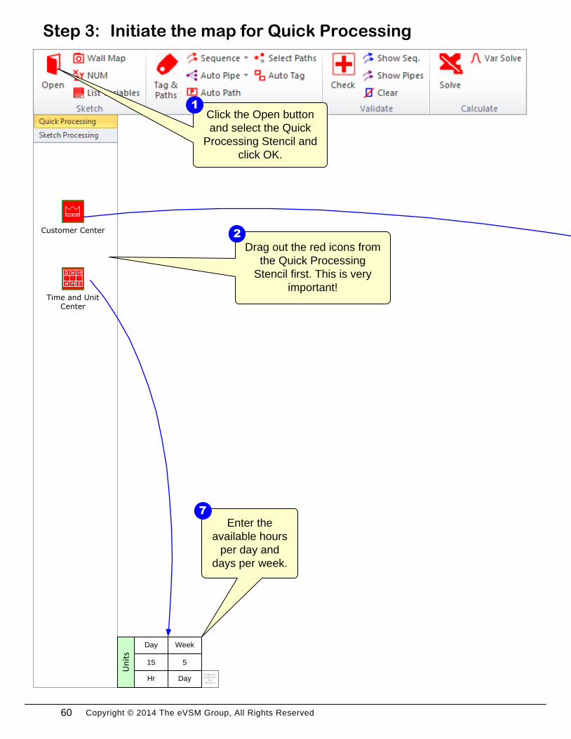
Initiate the map for Quick ProcessingStep 3:
Drag out the red icons from
the Quick Processing
Stencil first. This is very
important!
Enter the
available hours
per day and
days per week.
7
Click the Open button
and select the Quick
Processing Stencil and
click OK.
1
2
Time and Unit Center
Customer Center
eVSM Data
QuickProces
sing
7.30.0111.1
5
Week
Day
15
Day
Hr
Un
its
60
Copyright © 2014 The eVSM Group, All Rights Reserved
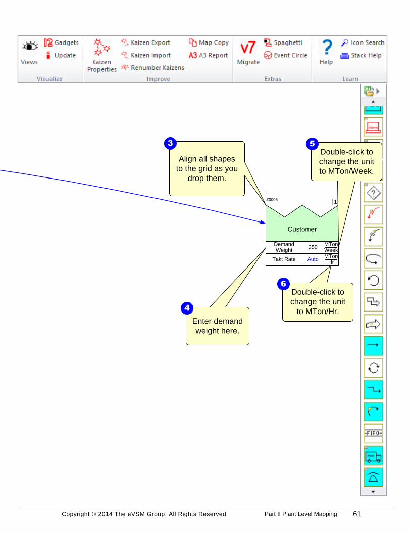
Initiate the map for Quick Processing
Align all shapes
to the grid as you
drop them.
3
Enter demand
weight here.
4
Takt RateMTon
HrAuto
Customer
Z00051
Demand Weight
MTonWeek
350
Double-click to
change the unit
to MTon/Week.
5
Double-click to
change the unit
to MTon/Hr.
6
61Part II Plant Level Mapping
Copyright © 2014 The eVSM Group, All Rights Reserved
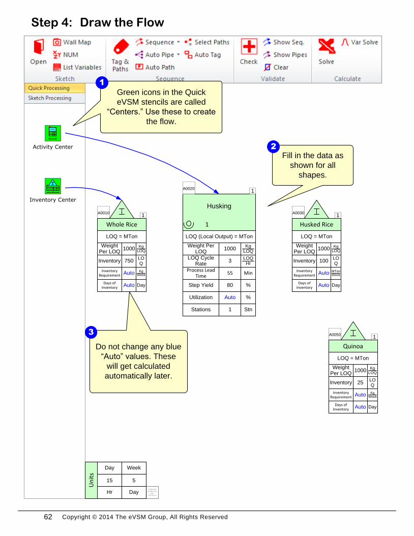
Draw the FlowStep 4:
Activity Center
Inventory Center
InventoryLOQ
750
LOQ = MTon
Weight Per LOQ
KgLOQ1000
A00101
Whole Rice
Inventory Requirement
KgWeekAuto
Days of Inventory
DayAuto
Husking
Utilization %Auto
1
LOQ (Local Output) = MTon
LOQ Cycle Rate
LOQHr
3
Weight Per LOQ
KgLOQ
1000
A00201
Step Yield %80
Process Lead Time
Min55
InventoryLOQ
100
LOQ = MTon
Weight Per LOQ
KgLOQ1000
A00301
Husked Rice
Inventory Requirement
MTonWeekAuto
Days of Inventory
DayAuto
InventoryLOQ
25
LOQ = MTon
Weight Per LOQ
KgLOQ1000
A00501
Quinoa
Inventory Requirement
KgWeekAuto
Days of Inventory
DayAuto
Green icons in the Quick
eVSM stencils are called
“Centers.” Use these to create
the flow.
1
Fill in the data as
shown for all
shapes.
2
Do not change any blue
“Auto” values. These
will get calculated
automatically later.
3
Stations Stn1
eVSM Data
QuickProces
sing
7.30.0111.1
5
Week
Day
15
Day
Hr
Un
its
62
Copyright © 2014 The eVSM Group, All Rights Reserved
Draw the Flow
Mixing & Packing
Utilization %Auto
1
LOQ (Local Output) = Bag
LOQ Cycle Rate
LOQHr
500
Weight Per LOQ
KgLOQ
25
A00601
Step Yield %100
Process Lead Time
Min25
InventoryLOQ
5000
LOQ = Bag
Weight Per LOQ
KgLOQ25
A00701
Enriched Grain
Inventory Requirement
KgWeekAuto
Days of Inventory
DayAuto
Takt RateMTon
HrAuto
Customer
Z00051
Demand Weight
MTonWeek
350
Stations Stn1
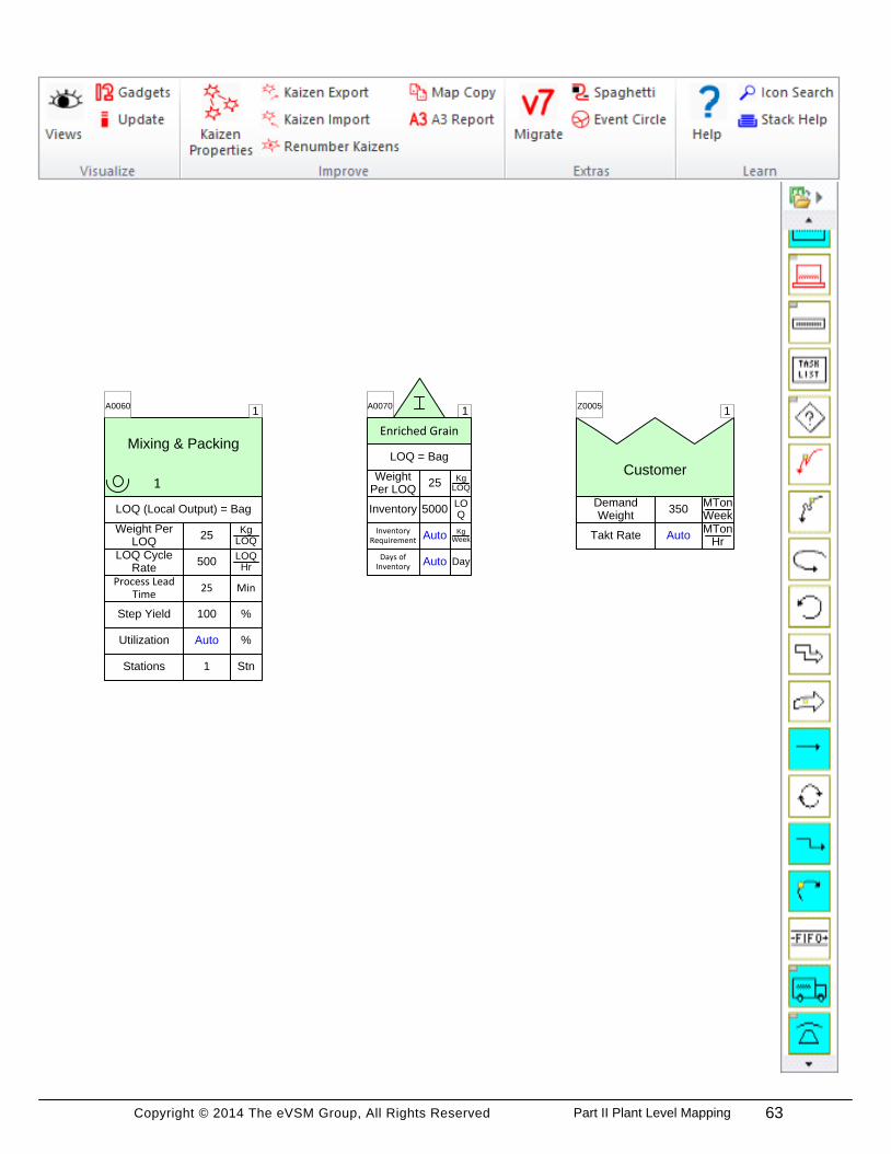
63Part II Plant Level Mapping
Copyright © 2014 The eVSM Group, All Rights Reserved
InventoryLOQ
750
LOQ = MTon
Weight Per LOQ
KgLOQ1000
A00101
Whole Rice
Inventory Requirement
KgWeekAuto
Days of Inventory
DayAuto
Husking
Utilization %Auto
1
LOQ (Local Output) = MTon
LOQ Cycle Rate
LOQHr
3
Weight Per LOQ
KgLOQ
1000
A00201
Step Yield %80
Process Lead Time
Min55
InventoryLOQ
100
LOQ = MTon
Weight Per LOQ
KgLOQ1000
A00301
Husked Rice
Inventory Requirement
MTonWeekAuto
Days of Inventory
DayAuto
InventoryLOQ
25
LOQ = MTon
Weight Per LOQ
KgLOQ1000
A00401
Quinoa
Inventory Requirement
KgWeekAuto
Days of Inventory
DayAuto
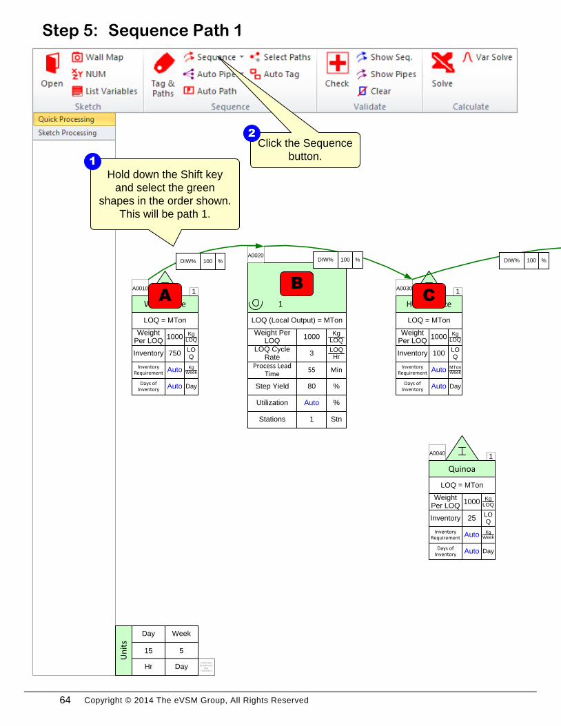
Sequence Path 1Step 5:
Hold down the Shift key
and select the green
shapes in the order shown.
This will be path 1.
1
Click the Sequence
button.
2
A
B
C
Stations Stn1
DIW% %100 DIW% %100 DIW% %100
eVSM Data
QuickProces
sing
7.30.0111.1
5
Week
Day
15
Day
Hr
Un
its
64
Copyright © 2014 The eVSM Group, All Rights Reserved
Mixing & Packing
Utilization %Auto
1
LOQ (Local Output) = Bag
LOQ Cycle Rate
LOQHr
500
Weight Per LOQ
KgLOQ
25
A00501
Step Yield %100
Process Lead Time
Min25
InventoryLOQ
5000
LOQ = Bag
Weight Per LOQ
KgLOQ25
A00601
Enriched Grain
Inventory Requirement
KgWeekAuto
Days of Inventory
DayAuto
Takt RateMTon
HrAuto
Customer
Z00051
Demand Weight
MTonWeek
350
Sequence Path 1
D
E
F
Stations Stn1
DIW% %100 DIW% %100
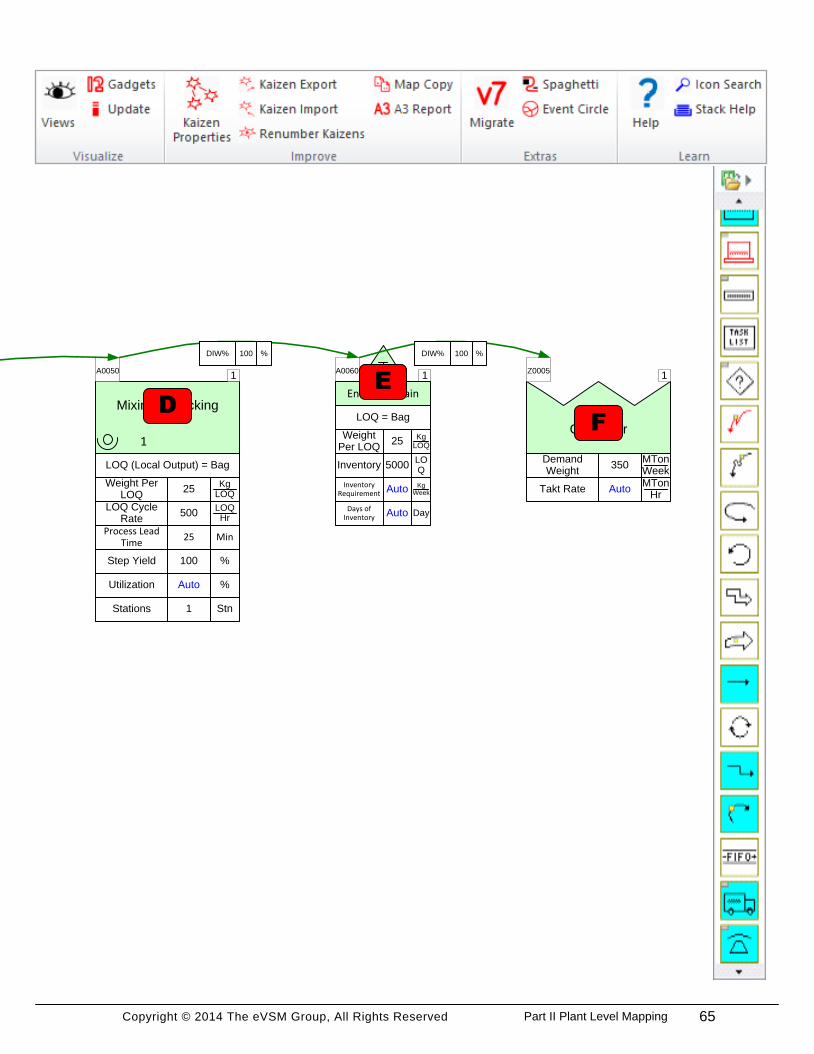
65Part II Plant Level Mapping
Copyright © 2014 The eVSM Group, All Rights Reserved
InventoryLOQ
750
LOQ = MTon
Weight Per LOQ
KgLOQ1000
A00101
Whole Rice
Inventory Requirement
KgWeekAuto
Days of Inventory
DayAuto
Husking
Utilization %Auto
1
LOQ (Local Output) = MTon
LOQ Cycle Rate
LOQHr
3
Weight Per LOQ
KgLOQ
1000
A00201
Step Yield %80
Process Lead Time
Min55
InventoryLOQ
100
LOQ = MTon
Weight Per LOQ
KgLOQ1000
A00301
Husked Rice
Inventory Requirement
MTonWeekAuto
Days of Inventory
DayAuto
InventoryLOQ
25
LOQ = MTon
Weight Per LOQ
KgLOQ1000
A00401
Quinoa
Inventory Requirement
KgWeekAuto
Days of Inventory
DayAuto
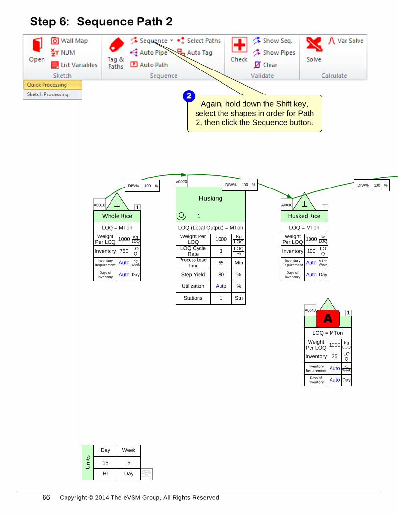
Sequence Path 2Step 6:
Again, hold down the Shift key,
select the shapes in order for Path
2, then click the Sequence button.
2
A
Stations Stn1
DIW% %100 DIW% %100 DIW% %100
eVSM Data
QuickProces
sing
7.30.0111.1
5
Week
Day
15
Day
Hr
Un
its
66
Copyright © 2014 The eVSM Group, All Rights Reserved
Mixing & Packing
Utilization %Auto
1
LOQ (Local Output) = Bag
LOQ Cycle Rate
LOQHr
500
Weight Per LOQ
KgLOQ
25
A00501
Step Yield %100
Process Lead Time
Min25
InventoryLOQ
5000
LOQ = Bag
Weight Per LOQ
KgLOQ25
A00601
Enriched Grain
Inventory Requirement
KgWeekAuto
Days of Inventory
DayAuto
Takt RateMTon
HrAuto
Customer
Z00051
Demand Weight
MTonWeek
350
Sequence Path 2
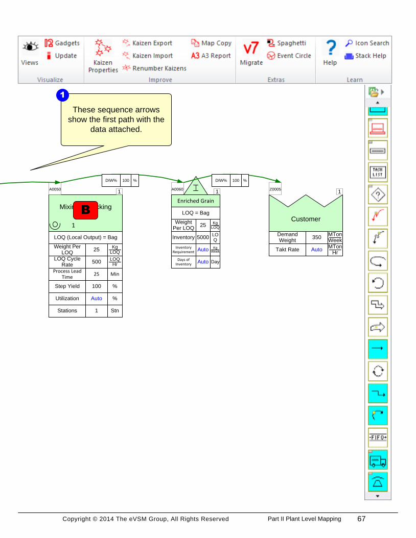
These sequence arrows
show the first path with the
data attached.
1
B
Stations Stn1
DIW% %100 DIW% %100
67Part II Plant Level Mapping
Copyright © 2014 The eVSM Group, All Rights Reserved
InventoryLOQ
750
LOQ = MTon
Weight Per LOQ
KgLOQ1000
A0010
Whole Rice
Inventory Requirement
KgWeekAuto
Days of Inventory
DayAuto
Husking
Utilization %Auto
1
LOQ (Local Output) = MTon
LOQ Cycle Rate
LOQHr
3
Weight Per LOQ
KgLOQ
1000
A0020
Step Yield %80
Process Lead Time
Min55
InventoryLOQ
100
LOQ = MTon
Weight Per LOQ
KgLOQ1000
A0030
Husked Rice
Inventory Requirement
MTonWeekAuto
Days of Inventory
DayAuto
InventoryLOQ
25
LOQ = MTon
Weight Per LOQ
KgLOQ1000
A0040
Quinoa
Inventory Requirement
KgWeekAuto
Days of Inventory
DayAuto
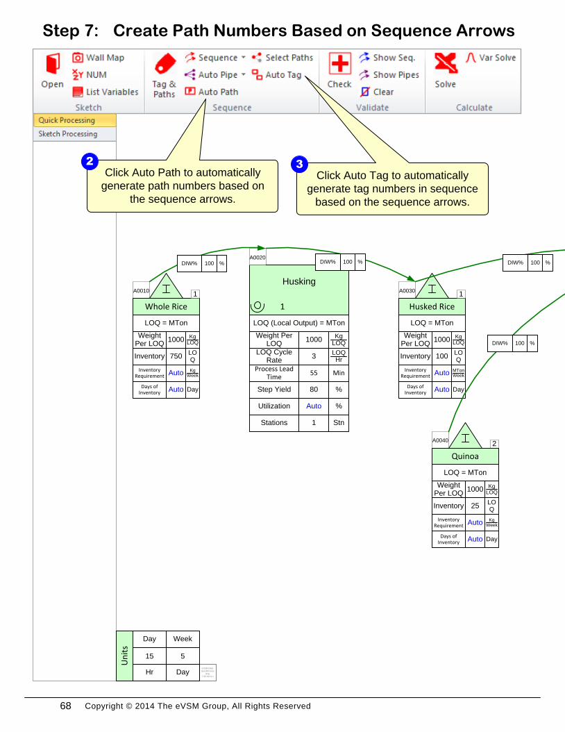
Step 7:
Click Auto Path to automatically
generate path numbers based on
the sequence arrows.
2
1
1
1
2
Create Path Numbers Based on Sequence Arrows
Stations Stn1
DIW% %100 DIW% %100 DIW% %100
DIW% %100
Click Auto Tag to automatically
generate tag numbers in sequence
based on the sequence arrows.
3
eVSM Data
QuickProces
sing
7.30.0111.1
5
Week
Day
15
Day
Hr
Un
its
68
Copyright © 2014 The eVSM Group, All Rights Reserved
Mixing & Packing
Utilization %Auto
1
LOQ (Local Output) = Bag
LOQ Cycle Rate
LOQHr
500
Weight Per LOQ
KgLOQ
25
A0050
Step Yield %100
Process Lead Time
Min25
InventoryLOQ
5000
LOQ = Bag
Weight Per LOQ
KgLOQ25
A0060
Enriched Grain
Inventory Requirement
KgWeekAuto
Days of Inventory
DayAuto
Takt RateMTon
HrAuto
Customer
Z0005
Demand Weight
MTonWeek
350
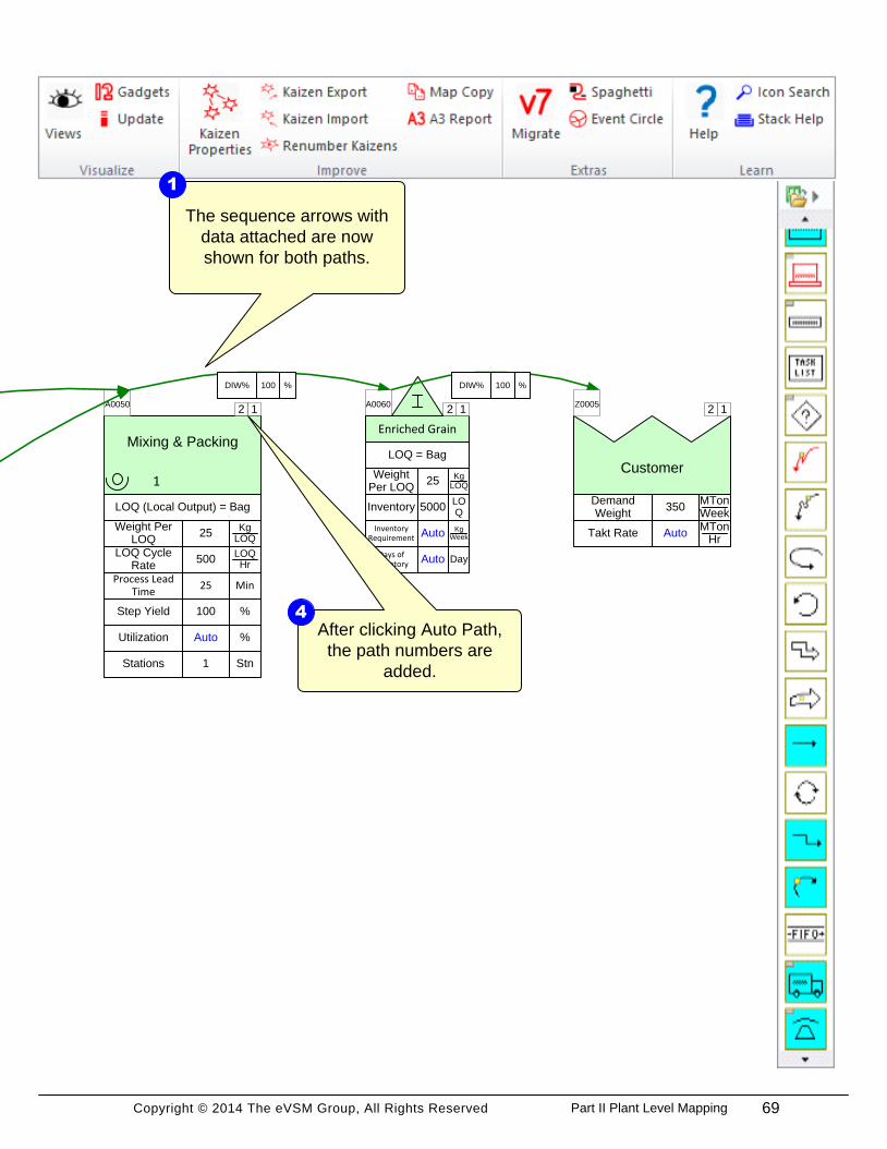
The sequence arrows with
data attached are now
shown for both paths.
1
After clicking Auto Path,
the path numbers are
added.
4
12 12 12
Create Path Numbers Based on Sequence Arrows
Stations Stn1
DIW% %100 DIW% %100
69Part II Plant Level Mapping
Copyright © 2014 The eVSM Group, All Rights Reserved
InventoryLOQ
750
LOQ = MTon
Weight Per LOQ
KgLOQ1000
A0010
Whole Rice
Inventory Requirement
KgWeekAuto
Days of Inventory
DayAuto
Husking
Utilization %Auto
1
LOQ (Local Output) = MTon
LOQ Cycle Rate
LOQHr
3
Weight Per LOQ
KgLOQ
1000
A0020
Step Yield %80
Process Lead Time
Min55
InventoryLOQ
100
LOQ = MTon
Weight Per LOQ
KgLOQ1000
A0030
Husked Rice
Inventory Requirement
MTonWeekAuto
Days of Inventory
DayAuto
InventoryLOQ
25
LOQ = MTon
Weight Per LOQ
KgLOQ1000
A0040
Quinoa
Inventory Requirement
KgWeekAuto
Days of Inventory
DayAuto
1
1
1
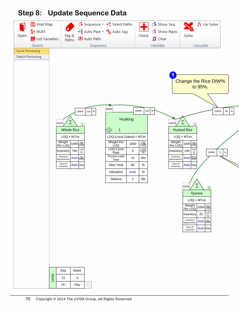
Change the Quinoa
DIW% to 5%.
Change the Rice DIW%
to 95%.
2
Update Sequence DataStep 8:
1
Stations Stn1
DIW% %100 DIW% %100 DIW% %95
DIW% %5
eVSM Data
QuickProces
sing
7.30.0111.1
5
Week
Day
15
Day
Hr
Un
its
70
Copyright © 2014 The eVSM Group, All Rights Reserved
Stations Stn1
Mixing & Packing
Utilization %Auto
1
LOQ (Local Output) = Bag
LOQ Cycle Rate
LOQHr
500
Weight Per LOQ
KgLOQ
25
A0050
Step Yield %100
Process Lead Time
Min25
InventoryLOQ
5000
LOQ = Bag
Weight Per LOQ
KgLOQ25
A0060
Enriched Grain
Inventory Requirement
KgWeekAuto
Days of Inventory
DayAuto
Takt RateMTon
HrAuto
Customer
Z0005
Demand Weight
MTonWeek
350
12 12 1
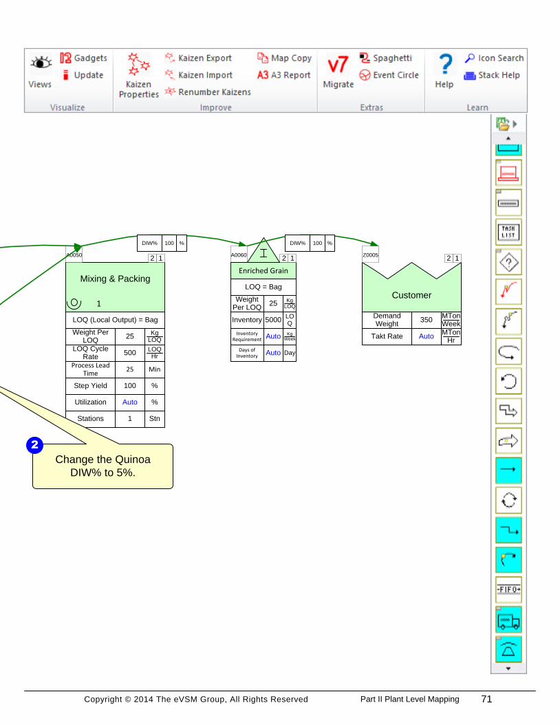
Change the Quinoa
DIW% to 5%.
2
Update Sequence Data
2
DIW% %100 DIW% %100
71Part II Plant Level Mapping
Copyright © 2014 The eVSM Group, All Rights Reserved
InventoryLOQ
750
LOQ = MTon
Weight Per LOQ
KgLOQ1000
A0010
Whole Rice
Inventory Requirement
MTonWeekAuto
Days of Inventory
DayAuto
Husking
Utilization %Auto
1
LOQ (Local Output) = MTon
LOQ Cycle Rate
LOQHr
3
Weight Per LOQ
KgLOQ
1000
A0020
Step Yield %80
Process Lead Time
Min55
InventoryLOQ
100
LOQ = MTon
Weight Per LOQ
KgLOQ1000
A0030
Husked Rice
Inventory Requirement
MTonWeekAuto
Days of Inventory
DayAuto
InventoryLOQ
25
LOQ = MTon
Weight Per LOQ
KgLOQ1000
A0040
Quinoa
Inventory Requirement
MTonWeekAuto
Days of Inventory
DayAuto
1
1
1
2
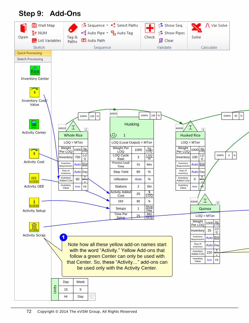
Add-OnsStep 9:
Double click to change
the unit to $/MTon on all
Inventory centers.
Inventory Center
Inventory Cost/Value
Inventory Added Cost
$MTo
n60
Inventory Value
K$Auto
Activity Center
Activity Cost
Activity OEE
Activity Setup
Activity Added Cost
$LOQ
25
OEE %80
SetupsStUpDay
1
Time Per Setup
MinStUp
25
Stations Stn2
Inventory Added Cost
$MTo
n220
Inventory Value
K$Auto
Inventory Added Cost
$MTo
n0
Inventory Value
K$Auto
Activity Scrap
Note how all these yellow add-on names start
with the word “Activity.” Yellow Add-ons that
follow a green Center can only be used with
that Center. So, these “Activity…” add-ons can
be used only with the Activity Center.
1
DIW% %100 DIW% %100 DIW% %95
DIW% %5
eVSM Data
QuickProces
sing
7.30.0111.1
5
Week
Day
15
Day
Hr
Un
its
72
Copyright © 2014 The eVSM Group, All Rights Reserved
Mixing & Packing
Utilization %Auto
1
LOQ (Local Output) = Bag
LOQ Cycle Rate
LOQHr
500
Weight Per LOQ
KgLOQ
25
A0050
Step Yield %100
Process Lead Time
Min25
InventoryLOQ
5000
LOQ = Bag
Weight Per LOQ
KgLOQ25
A0060
Enriched Grain
Inventory Requirement
MTonWeekAuto
Days of Inventory
DayAuto
Takt RateMTon
HrAuto
Customer
Z0005
Demand Weight
MTonWeek
350
12 12 12
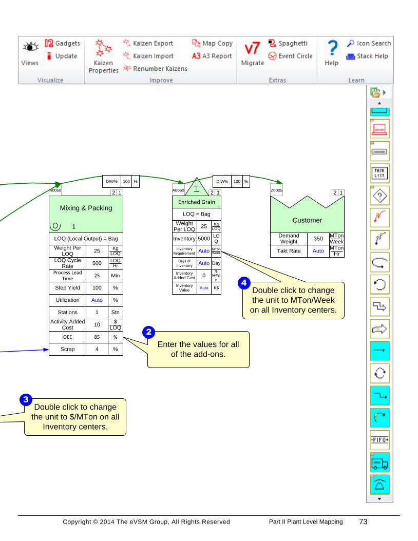
Add-Ons
Double click to change
the unit to $/MTon on all
Inventory centers.
3
Inventory Added Cost
$MTo
n0
Inventory Value
K$Auto
Activity Added Cost
$LOQ
10
OEE %85
Double click to change
the unit to MTon/Week
on all Inventory centers.
Enter the values for all
of the add-ons.
2
4
Scrap %4
Stations Stn1
DIW% %100 DIW% %100
73Part II Plant Level Mapping
Copyright © 2014 The eVSM Group, All Rights Reserved
InventoryLOQ
750
LOQ = MTon
Weight Per LOQ
KgLOQ1000
A0010
Whole Rice
Inventory Requirement
MTonWeek
432.94
Days of Inventory
Day8.66
Husking
Utilization %96.21
1
LOQ (Local Output) = MTon
LOQ Cycle Rate
LOQHr
3
Weight Per LOQ
KgLOQ
1000
A0020
Step Yield %80
Process Lead Time
Min55
InventoryLOQ
100
LOQ = MTon
Weight Per LOQ
KgLOQ1000
A0030
Husked Rice
Inventory Requirement
MTonWeek
346.35
Days of Inventory
Day1.44
InventoryLOQ
25
LOQ = MTon
Weight Per LOQ
KgLOQ1000
A0040
Quinoa
Inventory Requirement
MTonWeek18.23
Days of Inventory
Day6.86
1
1
1
2
Inventory Added Cost
$MTo
n60
Inventory Value
K$45.00
Activity Added Cost
$LOQ
25
OEE %80
SetupsStUpDay
1
Time Per Setup
MinStUp
25
Stations Stn2
Inventory Added Cost
$MTo
n220
Inventory Value
K$5.50
Inventory Added Cost
$MTo
n0
Inventory Value
K$10.00
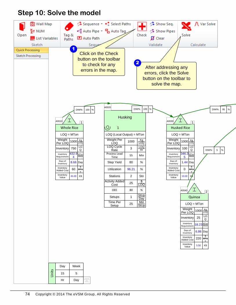
Click on the Check
button on the toolbar
to check for any
errors in the map.
1
After addressing any
errors, click the Solve
button on the toolbar to
solve the map.
2
Solve the modelStep 10:
DIW% %100 DIW% %100 DIW% %95
DIW% %5
eVSM Data
QuickProces
sing
7.30.0111.1
5
Week
Day
15
Day
Hr
Un
its
74
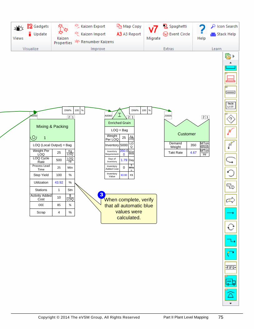
Copyright © 2014 The eVSM Group, All Rights Reserved
Mixing & Packing
Utilization %43.92
1
LOQ (Local Output) = Bag
LOQ Cycle Rate
LOQHr
500
Weight Per LOQ
KgLOQ
25
A0050
Step Yield %100
Process Lead Time
Min25
InventoryLOQ
5000
LOQ = Bag
Weight Per LOQ
KgLOQ25
A0060
Enriched Grain
Inventory Requirement
MTonWeek
350.00
Days of Inventory
Day1.79
Takt RateMTon
Hr4.67
Customer
Z0005
Demand Weight
MTonWeek
350
12 12 12
Inventory Added Cost
$MTo
n0
Inventory Value
K$63.80
Activity Added Cost
$LOQ
10
OEE %85
When complete, verify
that all automatic blue
values were
calculated.
3
Solve the model
Scrap %4
Stations Stn1
DIW% %100 DIW% %100
75Part II Plant Level Mapping
Copyright © 2014 The eVSM Group, All Rights Reserved
InventoryLOQ
750
LOQ = MTon
Weight Per LOQ
KgLOQ1000
A0010
Whole Rice
Inventory Requirement
MTonWeek
432.94
Days of Inventory
Day8.66
Husking
Utilization %96.21
1
LOQ (Local Output) = MTon
LOQ Cycle Rate
LOQHr
3
Weight Per LOQ
KgLOQ
1000
A0020
Step Yield %80
Process Lead Time
Min55
InventoryLOQ
100
LOQ = MTon
Weight Per LOQ
KgLOQ1000
A0030
Husked Rice
Inventory Requirement
MTonWeek
346.35
Days of Inventory
Day1.44
InventoryLOQ
25
LOQ = MTon
Weight Per LOQ
KgLOQ1000
A0040
Quinoa
Inventory Requirement
MTonWeek18.23
Days of Inventory
Day6.86
1
1
1
2
Inventory Added Cost
$MTo
n60
Inventory Value
K$45.00
Activity Added Cost
$LOQ
25
OEE %80
SetupsStUpDay
1
Time Per Setup
MinStUp
25
Stations Stn2
Inventory Added Cost
$MTo
n220
Inventory Value
K$5.50
Inventory Added Cost
$MTo
n0
Inventory Value
K$10.00
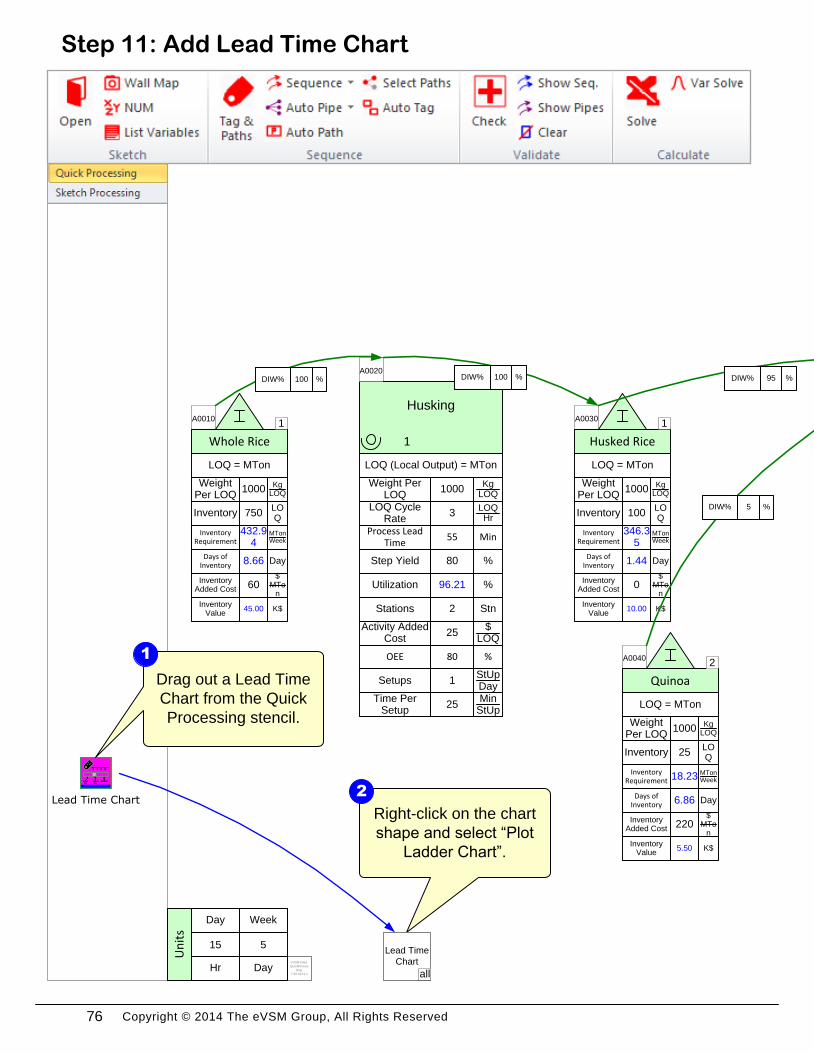
Add Lead Time ChartStep 11:
Right-click on the chart
shape and select “Plot
Ladder Chart”.
2Lead Time Chart
Drag out a Lead Time
Chart from the Quick
Processing stencil.
1
DIW% %100 DIW% %100 DIW% %95
DIW% %5
Lead Time
Chart
all
eVSM Data
QuickProces
sing
7.30.0111.1
5
Week
Day
15
Day
Hr
Un
its
76
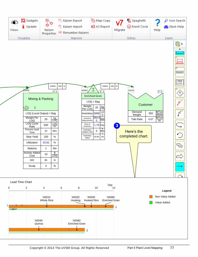
Copyright © 2014 The eVSM Group, All Rights Reserved
Mixing & Packing
Utilization %43.92
1
LOQ (Local Output) = Bag
LOQ Cycle Rate
LOQHr
500
Weight Per LOQ
KgLOQ
25
A0050
Step Yield %100
Process Lead Time
Min25
InventoryLOQ
5000
LOQ = Bag
Weight Per LOQ
KgLOQ25
A0060
Enriched Grain
Inventory Requirement
MTonWeek
350.00
Days of Inventory
Day1.79
Takt RateMTon
Hr4.67
Customer
Z0010
Demand Weight
MTonWeek
350
12 12 12
Inventory Added Cost
$MTo
n0
Inventory Value
K$63.80
Activity Added Cost
$LOQ
10
OEE %85
Scrap %4
Add Lead Time Chart
Here’s the
completed chart.
3
Stations Stn1
DIW% %100 DIW% %100
Lead Time ChartDay
0 2 4 6 8 10 12
'A0010
Whole Rice
'A0020
Husking
'A0030
Husked Rice
'A0060
Enriched Grain
11.67
'A0040
Quinoa
'A0060
Enriched Grain
2
1.00
Non Value Added
Legend
Value Added
77Part II Plant Level Mapping
Copyright © 2014 The eVSM Group, All Rights Reserved
InventoryLOQ
750
LOQ = MTon
Weight Per LOQ
KgLOQ1000
A0010
Whole Rice
Inventory Requirement
MTonWeek
432.94
Days of Inventory
Day8.66
Husking
Utilization %96.21
1
LOQ (Local Output) = MTon
LOQ Cycle Rate
LOQHr
3
Weight Per LOQ
KgLOQ
1000
A0020
Step Yield %80
Process Lead Time
Min55
InventoryLOQ
100
LOQ = MTon
Weight Per LOQ
KgLOQ1000
A0030
Husked Rice
Inventory Requirement
MTonWeek
346.35
Days of Inventory
Day1.44
InventoryLOQ
25
LOQ = MTon
Weight Per LOQ
KgLOQ1000
A0040
Quinoa
Inventory Requirement
MTonWeek18.23
Days of Inventory
Day6.86
1
1
1
2
Inventory Added Cost
$MTo
n60
Inventory Value
K$45.00
Activity Added Cost
$LOQ
25
OEE %80
SetupsStUpDay
1
Time Per Setup
MinStUp
25
Stations Stn2
Inventory Added Cost
$MTo
n220
Inventory Value
K$5.50
Inventory Added Cost
$MTo
n0
Inventory Value
K$10.00
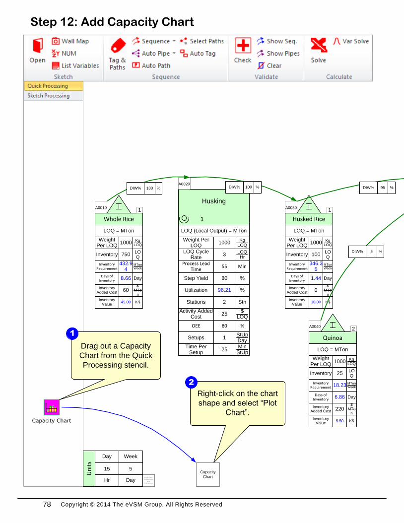
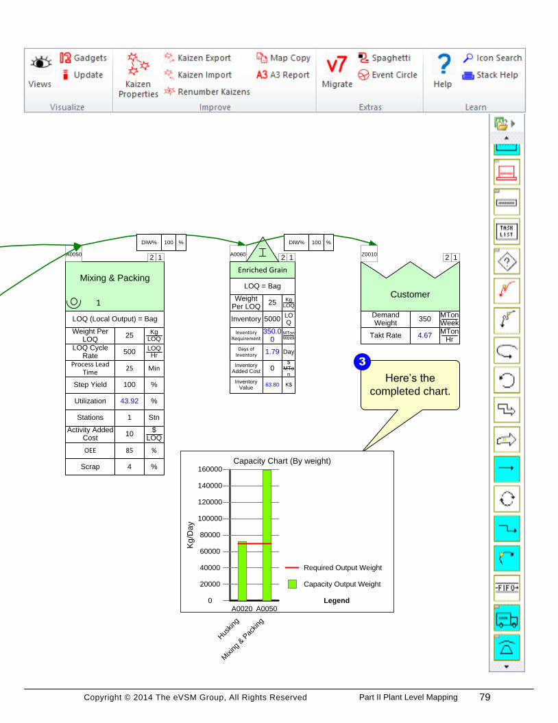
Capacity Chart
Right-click on the chart
shape and select “Plot
Chart”.
2
Drag out a Capacity
Chart from the Quick
Processing stencil.
1
Capacity
Chart
Add Capacity ChartStep 12:
DIW% %100 DIW% %100 DIW% %95
DIW% %5
eVSM Data
QuickProces
sing
7.30.0111.1
5
Week
Day
15
Day
Hr
Un
its
78
Copyright © 2014 The eVSM Group, All Rights Reserved
Mixing & Packing
Utilization %43.92
1
LOQ (Local Output) = Bag
LOQ Cycle Rate
LOQHr
500
Weight Per LOQ
KgLOQ
25
A0050
Step Yield %100
Process Lead Time
Min25
InventoryLOQ
5000
LOQ = Bag
Weight Per LOQ
KgLOQ25
A0060
Enriched Grain
Inventory Requirement
MTonWeek
350.00
Days of Inventory
Day1.79
Takt RateMTon
Hr4.67
Customer
Z0010
Demand Weight
MTonWeek
350
12 12 12
Inventory Added Cost
$MTo
n0
Inventory Value
K$63.80
Activity Added Cost
$LOQ
10
OEE %85
Scrap %4
Here’s the
completed chart.
3
Add Capacity Chart
DIW% %100 DIW% %100
Capacity Chart (By weight)
Kg
/Da
y
0
20000
40000
60000
80000
100000
120000
140000
160000
A0020
Hus
king
A0050
Mixing
& P
acking
Capacity Output Weight
Legend
Required Output Weight
Stations Stn1
79Part II Plant Level Mapping
Copyright © 2014 The eVSM Group, All Rights Reserved
InventoryLOQ
750
LOQ = MTon
Weight Per LOQ
KgLOQ1000
A0010
Whole Rice
Inventory Requirement
MTonWeek
432.94
Days of Inventory
Day8.66
Husking
Utilization %96.21
1
LOQ (Local Output) = MTon
LOQ Cycle Rate
LOQHr
3
Weight Per LOQ
KgLOQ
1000
A0020
Step Yield %80
Process Lead Time
Min55
InventoryLOQ
100
LOQ = MTon
Weight Per LOQ
KgLOQ1000
A0030
Husked Rice
Inventory Requirement
MTonWeek
346.35
Days of Inventory
Day1.44
InventoryLOQ
25
LOQ = MTon
Weight Per LOQ
KgLOQ1000
A0040
Quinoa
Inventory Requirement
MTonWeek18.23
Days of Inventory
Day6.86
1
1
1
2
Inventory Added Cost
$MTo
n60
Inventory Value
K$45.00
Activity Added Cost
$LOQ
25
OEE %80
SetupsStUpDay
1
Time Per Setup
MinStUp
25
Stations Stn2
Inventory Added Cost
$MTo
n220
Inventory Value
K$5.50
Inventory Added Cost
$MTo
n0
Inventory Value
K$10.00
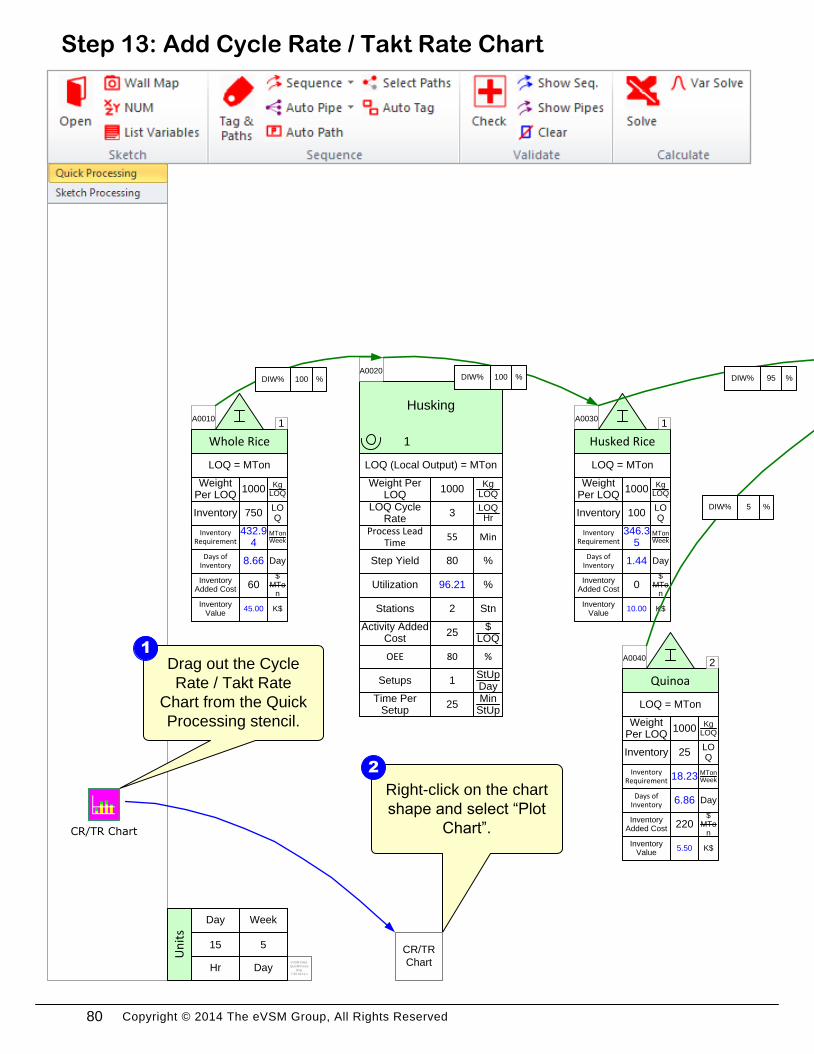
Add Cycle Rate / Takt Rate ChartStep 13:
Right-click on the chart
shape and select “Plot
Chart”.
2
Drag out the Cycle
Rate / Takt Rate
Chart from the Quick
Processing stencil.
1
CR/TR Chart
CR/TR
Chart
DIW% %100 DIW% %100 DIW% %95
DIW% %5
eVSM Data
QuickProces
sing
7.30.0111.1
5
Week
Day
15
Day
Hr
Un
its
80
Copyright © 2014 The eVSM Group, All Rights Reserved
Mixing & Packing
Utilization %43.92
1
LOQ (Local Output) = Bag
LOQ Cycle Rate
LOQHr
500
Weight Per LOQ
KgLOQ
25
A0050
Step Yield %100
Process Lead Time
Min25
InventoryLOQ
5000
LOQ = Bag
Weight Per LOQ
KgLOQ25
A0060
Enriched Grain
Inventory Requirement
MTonWeek
350.00
Days of Inventory
Day1.79
Takt RateMTon
Hr4.67
Customer
Z0010
Demand Weight
MTonWeek
350
12 12 12
Inventory Added Cost
$MTo
n0
Inventory Value
K$63.80
Activity Added Cost
$LOQ
10
OEE %85
Scrap %4
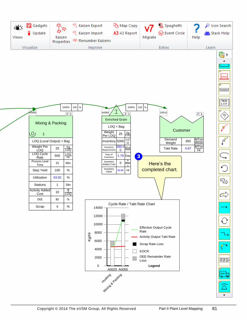
Add Cycle Rate / Takt Rate Chart
Here’s the
completed chart.
3
Stations Stn1
DIW% %100 DIW% %100
Cycle Rate / Takt Rate Chart
Kg
/Hr
0
2000
4000
6000
8000
10000
12000
14000
A0020
Hus
king
A0050
Mixing
& P
acking
OEE Remainder Rate
Loss
Legend
EOCR
Scrap Rate Loss
Activity Output Takt Rate
Effective Output Cycle
Rate
81Part II Plant Level Mapping
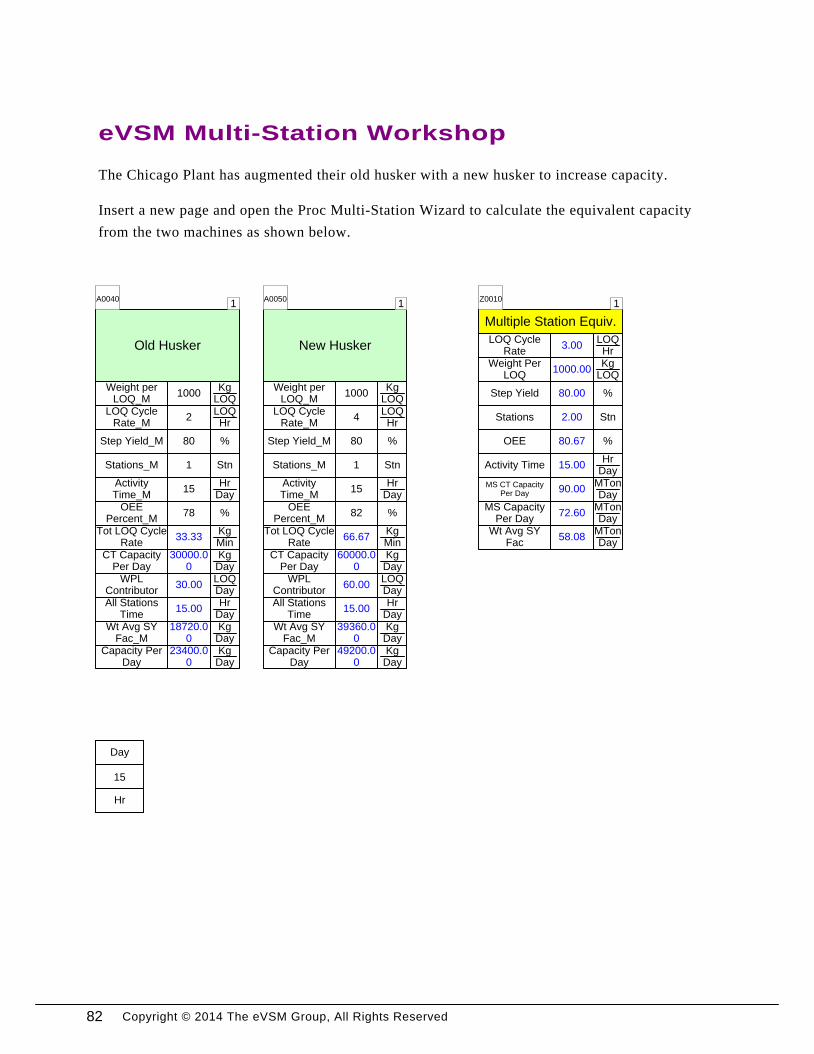
Copyright © 2014 The eVSM Group, All Rights Reserved
eVSM Multi-Station Workshop
The Chicago Plant has augmented their old husker with a new husker to increase capacity.
Insert a new page and open the Proc Multi-Station Wizard to calculate the equivalent capacity
from the two machines as shown below.
15
Day
Hr
Old Husker
1A0040
Step Yield_M %80
LOQ Cycle Rate_M
LOQHr
2
Tot LOQ Cycle Rate
KgMin
33.33
Stations_M Stn1
Activity Time_M
HrDay
15
OEE Percent_M
%78
CT Capacity Per Day
KgDay
30000.00
WPL Contributor
LOQDay
30.00
Weight per LOQ_M
KgLOQ
1000
All Stations Time
HrDay
15.00
Wt Avg SY Fac_M
KgDay
18720.00
Capacity Per Day
KgDay
23400.00
New Husker
1A0050
Step Yield_M %80
LOQ Cycle Rate_M
LOQHr
4
Tot LOQ Cycle Rate
KgMin
66.67
Stations_M Stn1
Activity Time_M
HrDay
15
OEE Percent_M
%82
CT Capacity Per Day
KgDay
60000.00
WPL Contributor
LOQDay
60.00
Weight per LOQ_M
KgLOQ
1000
All Stations Time
HrDay
15.00
Wt Avg SY Fac_M
KgDay
39360.00
Capacity Per Day
KgDay
49200.00
Multiple Station Equiv.
1Z0010
Stations Stn2.00
MS Capacity Per Day
MTonDay
72.60
Activity TimeHr
Day15.00
MS CT Capacity Per Day
MTonDay
90.00
OEE %80.67
Weight Per LOQ
KgLOQ
1000.00
LOQ Cycle Rate
LOQHr
3.00
Wt Avg SY Fac
MTonDay
58.08
Step Yield %80.00
82
Copyright © 2014 The eVSM Group, All Rights Reserved
In looking at the current value stream, there has been concern raised about the shelf-life impact
on the enriched rice product of holding large inventories of Quinoa and Whole Grain. It should
be easy to manage these stores to an average inventory of 5 days of supply each.
The husking process is running near capacity and often proves to be a bottleneck given variation
in demand and unpredictable downtime. Speeding up the equipment unfortunately seems to
increase the downtime. It seems important to both improve the cycle rate and the OEE of the
equipment here even though its expected to be a challenge.
You can envisage the above by first marking up the current state map
1. Add kaizen bursts to the map
2. Add impact/ease of implementation ratings to the bursts
3. Draw a Kaizen Impact matrix (See back index in eVSM User Guide)
4. Create a Kaizen Key and a Kaizen Report
Assuming that the improvements identified above are targeted to manage the inventories of both
the Quinoa and Whole Grain to an average 5 days and that the husking cycle rate is targeted to
improve to an average 3.5 MTons/Hr at each station, create a future state map that shows the
impact of the changes.
eVSM - Improvements Workshop
83Part II Plant Level Mapping
Copyright © 2014 The eVSM Group, All Rights Reserved
Chicago Rice – Resource Modeling
Exercise
With your group, read the information below and then:
1. Model the resources for the activity.
2. Show the data associated with the resource handling as well as resource pipe data.
3. Calculate the map.
4. Identify what charts would be useful to visualize the value stream and mark these up.
5. Identify where there is a bottleneck.
Background and Overview
Chicago Rice Inc. sells an enriched grain product which is made from a combination of rice and
quinoa. The plant line first husks the whole rice then mixes the rice with the quinoa as an
enriched grain product. You take a second value stream walk with the plant supervisor to model
the resource allocation for the activity processes.
Value Stream Walk
The plant supervisor explains how resources are coming from technicians as well as machines.
You first notice that the Husking activity has three different resources being piped into it. The
first is a maintenance technician who has a resource quantity of 1 and works 2 hours a day. His
setup time takes 60 minutes. The second is a Huskers machine running 15 hours a days with a
resource quantity of 2. It has a process time of 20 minutes and a setup time of 50 minutes.
The third resource is an operator who is being shared between the Husking activity and the
Mixing & Packing activity. That operator has a resource quantity of 2, and works 15 hours a day.
The resource process time for the Husking activity is 15 minutes per LOQ with a walk time of 1
minute. The resource process time is 10 seconds per LOQ with a 5 second walk time for the
Mixing & Packing activity. The Mixing & Packing has a second operator working 15 hours day
and a resource quantity of 1. The resource process time is 10 seconds per LOQ.
84
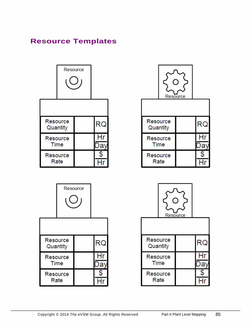
Copyright © 2014 The eVSM Group, All Rights Reserved
Resource Templates
85Part II Plant Level Mapping

Copyright © 2014 The eVSM Group, All Rights Reserved 86
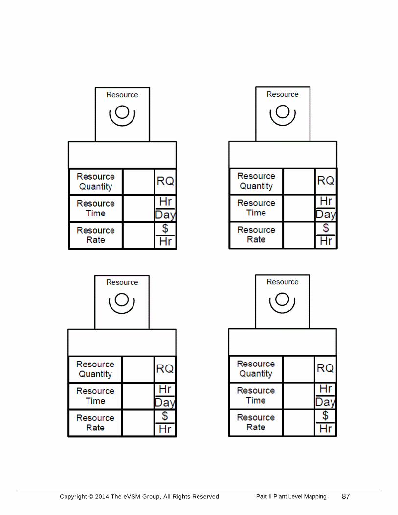
Copyright © 2014 The eVSM Group, All Rights Reserved 87Part II Plant Level Mapping

Copyright © 2014 The eVSM Group, All Rights Reserved 88

Copyright © 2014 The eVSM Group, All Rights Reserved
eVSM - Resource Workshop
1. Take the existing Plant map to add the resource centers to using the same Quick Processing
stencil.
2. Drag out a Resource Center and fill in the appropriate data.
3. Drag out the Resource Pipe and make sure to glue both ends of an operation tag.
4. Check the map and then Solve for the calculated fields.
5. Make the Walk Time and Setup Time visible using the Views button in the toolbar.
6. Draw the Resource Balance Chart.
89Part II Plant Level Mapping
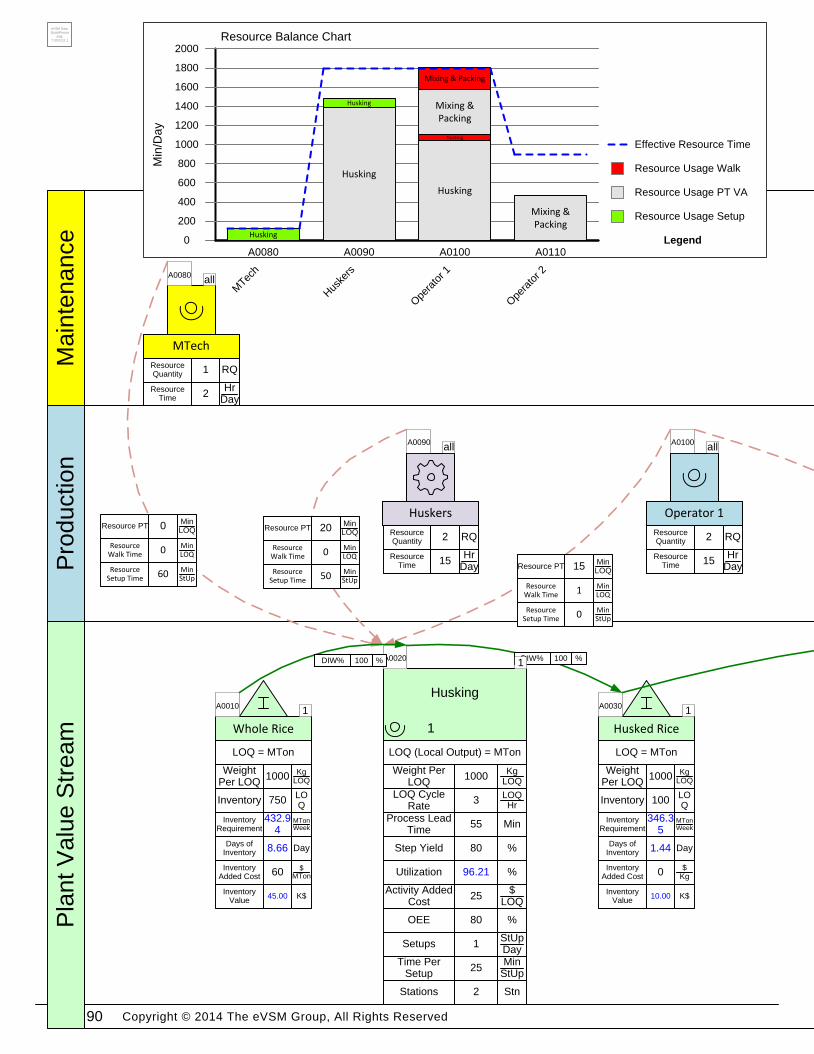
Copyright © 2014 The eVSM Group, All Rights Reserved
Ma
inte
na
nce
Pla
nt V
alu
e S
tre
am
Pro
du
ctio
n
Whole Rice
LOQ = MTon
InventoryLOQ
750
Weight Per LOQ
KgLOQ1000
Inventory Requirement
MTonWeek
432.94
Days of Inventory
Day8.66
A0010
Husking
1
LOQ (Local Output) = MTon
Utilization %96.21
LOQ Cycle Rate
LOQHr
3
Weight Per LOQ
KgLOQ
1000
Step Yield %80
Process Lead Time
Min55
A0020
Husked Rice
LOQ = MTon
InventoryLOQ
100
Weight Per LOQ
KgLOQ1000
Inventory Requirement
MTonWeek
346.35
Days of Inventory
Day1.44
A0030
MTech
Resource Time
HrDay
2
Resource Quantity RQ1
A0080all
Resource PTMinLOQ0
Huskers
Resource Time
HrDay
15
Resource Quantity RQ2
A0090all
Operator 1
Resource Time
HrDay
15
Resource Quantity RQ2
A0100all
Resource PTMinLOQ20
Resource PTMinLOQ15
Resource Walk Time
MinLOQ0
Resource Setup Time
MinStUp60
Resource Walk Time
MinLOQ0
Resource Setup Time
MinStUp50
Resource Walk Time
MinLOQ1
Resource Setup Time
MinStUp0
Inventory Added Cost
$MTon60
Inventory Value
K$45.00Activity Added
Cost$
LOQ25
OEE %80
SetupsStUpDay
1
Time Per Setup
MinStUp
25
Stations Stn2
Inventory Added Cost
$Kg0
Inventory Value
K$10.00
DIW% %100 DIW% %100
1
1
1
Resource
Balance
Resource Balance Chart
Min
/Da
y
0
200
400
600
800
1000
1200
1400
1600
1800
2000
A0080
MTec
h
A0090
Hus
kers
A0100
Ope
rato
r 1
A0110
Ope
rato
r 2
Husking
Husking
Husking
Husking
Husking
Mixing & Packing
Mixing & Packing
Mixing & Packing
Resource Usage Setup
Legend
Resource Usage PT VA
Resource Usage Walk
Effective Resource Time
eVSM Data
QuickProces
sing
7.30.0111.1
90
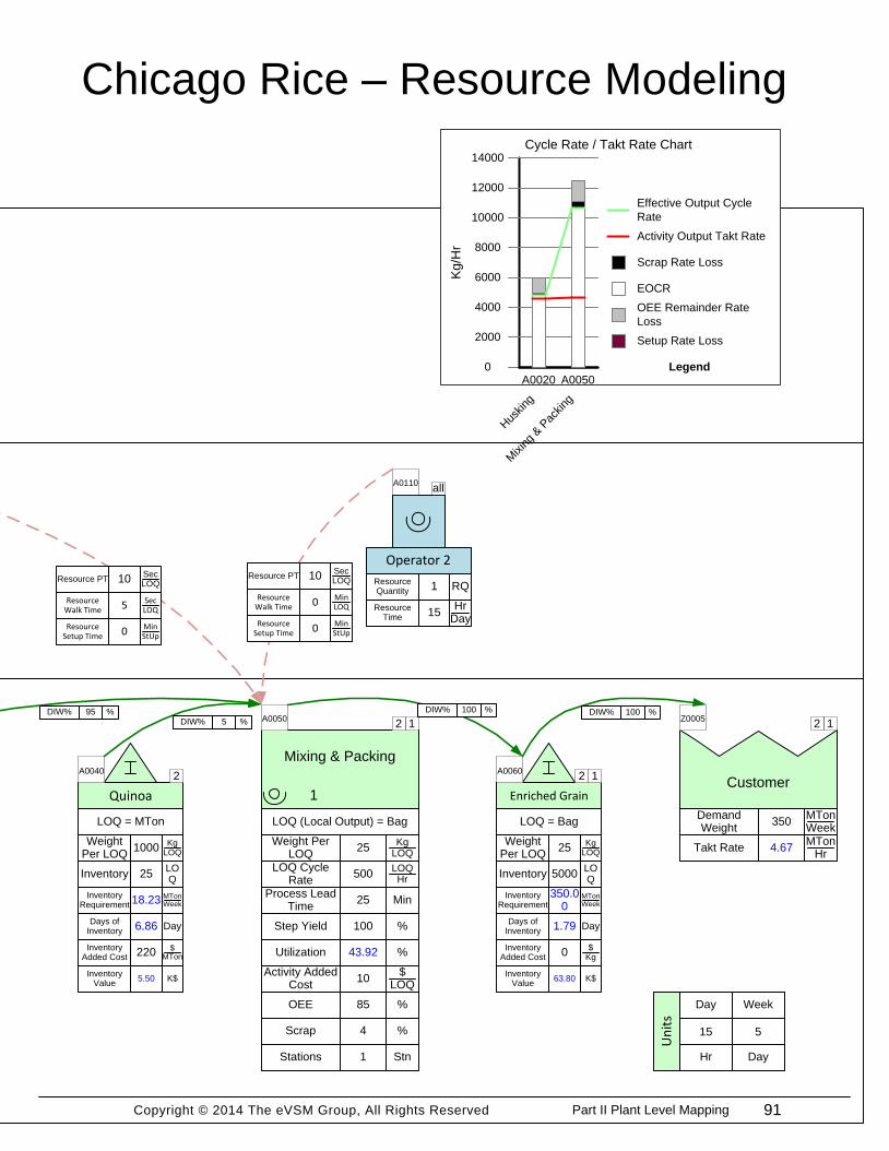
Copyright © 2014 The eVSM Group, All Rights Reserved
Chicago Rice – Resource Modeling
Quinoa
LOQ = MTon
InventoryLOQ
25
Weight Per LOQ
KgLOQ1000
Inventory Requirement
MTonWeek18.23
Days of Inventory
Day6.86
A0040
Mixing & Packing
1
LOQ (Local Output) = Bag
Utilization %43.92
LOQ Cycle Rate
LOQHr
500
Weight Per LOQ
KgLOQ
25
Step Yield %100
Process Lead Time
Min25
A0050
Enriched Grain
LOQ = Bag
InventoryLOQ
5000
Weight Per LOQ
KgLOQ25
Inventory Requirement
MTonWeek
350.00
Days of Inventory
Day1.79
A0060
Customer
Takt RateMTon
Hr4.67
Demand Weight
MTonWeek
350
Z0005
Operator 2
Resource Time
HrDay
15
Resource Quantity RQ1
A0110all
Resource PTSecLOQ10 Resource PT
SecLOQ10
Resource Walk Time
SecLOQ5
Resource Setup Time
MinStUp0
Resource Walk Time
MinLOQ0
Resource Setup Time
MinStUp0
Inventory Added Cost
$MTon220
Inventory Value
K$5.50Activity Added
Cost$
LOQ10
OEE %85
Scrap %4
Inventory Added Cost
$Kg0
Inventory Value
K$63.80
DIW% %95 DIW% %100 DIW% %100DIW% %5 12
12
12
2
CR/TR
Chart
Stations Stn1
Cycle Rate / Takt Rate Chart
Kg
/Hr
0
2000
4000
6000
8000
10000
12000
14000
A0020
Hus
king
A0050
Mixing
& P
acking
Setup Rate Loss
Legend
OEE Remainder Rate
Loss
EOCR
Scrap Rate Loss
Activity Output Takt Rate
Effective Output Cycle
Rate
5
Week
Day
15
Day
Hr
Un
its
91Part II Plant Level Mapping

Copyright © 2014 The eVSM Group, All Rights Reserved 92
Copyright © 2014 The eVSM Group, All Rights Reserved
Part III: Inbound and Outbound Maps
Chicago Rice Inc. sells an enriched grain product which is made from a combination of rice and
quinoa. First, the company receives shipments of whole rice from two suppliers and a shipment
of quinoa from one supplier. Next, in the plant the rice is husked and combined with the quinoa
to form an enriched grain product. Finally, the grain is shipped to two warehouses and then
distributed to the two customers.
93Part III Inbound and Outbound Maps
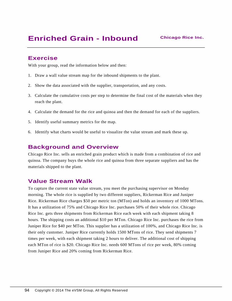
Copyright © 2014 The eVSM Group, All Rights Reserved
Enriched Grain - Inbound Chicago Rice Inc.
Exercise
With your group, read the information below and then:
1. Draw a wall value stream map for the inbound shipments to the plant.
2. Show the data associated with the supplier, transportation, and any costs.
3. Calculate the cumulative costs per step to determine the final cost of the materials when they
reach the plant.
4. Calculate the demand for the rice and quinoa and then the demand for each of the suppliers.
5. Identify useful summary metrics for the map.
6. Identify what charts would be useful to visualize the value stream and mark these up.
Background and Overview
Chicago Rice Inc. sells an enriched grain product which is made from a combination of rice and
quinoa. The company buys the whole rice and quinoa from three separate suppliers and has the
materials shipped to the plant.
Value Stream Walk
To capture the current state value stream, you meet the purchasing supervisor on Monday
morning. The whole rice is supplied by two different suppliers, Rickerman Rice and Juniper
Rice. Rickerman Rice charges $50 per metric ton (MTon) and holds an inventory of 1000 MTons.
It has a utilization of 75% and Chicago Rice Inc. purchases 50% of their whole rice. Chicago
Rice Inc. gets three shipments from Rickerman Rice each week with each shipment taking 8
hours. The shipping costs an additional $10 per MTon. Chicago Rice Inc. purchases the rice from
Juniper Rice for $40 per MTon. This supplier has a utilization of 100%, and Chicago Rice Inc. is
their only customer. Juniper Rice currently holds 1500 MTons of rice. They send shipments 7
times per week, with each shipment taking 2 hours to deliver. The additional cost of shipping
each MTon of rice is $20. Chicago Rice Inc. needs 600 MTons of rice per week, 80% coming
from Juniper Rice and 20% coming from Rickerman Rice.
94
Copyright © 2014 The eVSM Group, All Rights Reserved
The quinoa is supplied by Quaker Quinoa at a cost of $200 per MTon. Quaker Quinoa has a
utilization of 75% and Chicago Rice Inc. purchases 40% share of their quinoa. This supplier
currently holds 20 MTons of quinoa at their warehouse and sends out shipments once a week.
Each shipment takes 5 hours to reach Chicago Quinoa and adds an additional cost of $20 per
MTon. The Chicago Rice Inc. needs 20 MTons of quinoa per week.
95Part III Inbound and Outbound Maps
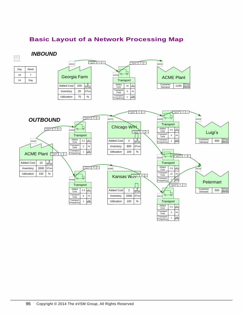
Copyright © 2014 The eVSM Group, All Rights Reserved
Basic Layout of a Network Processing Map
Georgia Farm
A0010
Added Cost$
STon200
Inventory STon20
Utilization %75
eVSM Data
QuickProces
singNetwork
7.02.0002.2
24
Day
Hr
7
Week
DayACME Plant
A0020
Customer Demand
STonWeek
1100
Transport
Added Cost
$STon20
A0030
Transport Time
Hr5
Transport Frequency
TripWeek1
Downstream Input %
%100 Downstream Input %
%100
ACME Plant
A0040
Added Cost$
STon10
Inventory STon2000
Utilization %100
Transport
Added Cost
$STon0.2
A0050
Transport Time
Hr2
Transport Frequency
TripWeek1
Transport
Added Cost
$STon0.3
A0060
Transport Time
Hr8
Transport Frequency
TripWeek1
Chicago W/H
A0070
Added Cost$
STon2
Inventory STon800
Utilization %100
Kansas W/H
A0080
Added Cost$
STon2
Inventory STon2000
Utilization %100
Transport
Added Cost
$STon0.5
A0090
Transport Time
Hr4
Transport Frequency
TripWeek1
Transport
Added Cost
$STon0.9
A0100
Transport Time
Hr12
Transport Frequency
TripWeek1
Transport
Added Cost
$STon0.2
A0110
Transport Time
Hr3
Transport Frequency
TripWeek1
Luigi’s
A0120
Customer Demand
STonWeek
600
Petermart
A0130
Customer Demand
STonWeek
500
Downstream Input %
%100
Downstream Input %
%100
Downstream Input %
%100Downstream
Input %%100
Downstream Input %
%100
Downstream Input %
%20
Downstream Input %
%100
Downstream Input %
%100
Downstream Input %
%100
Downstream Input %
%80
INBOUND
OUTBOUND
96
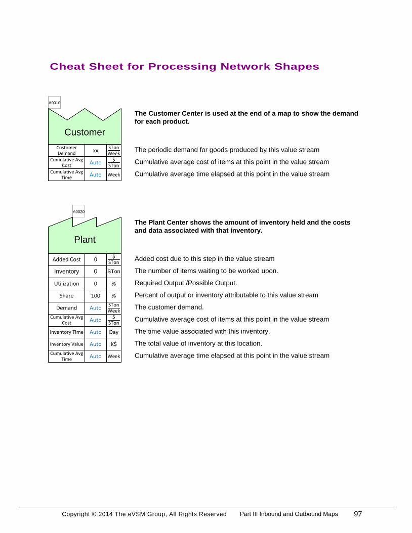
Copyright © 2014 The eVSM Group, All Rights Reserved
Cheat Sheet for Processing Network Shapes
Customer
A0010
Customer Demand
STonWeek
xx
Cumulative Avg Cost
$STon
Auto
Cumulative Avg Time
WeekAuto
The periodic demand for goods produced by this value stream
Cumulative average cost of items at this point in the value stream
Cumulative average time elapsed at this point in the value stream
Plant
A0020
DemandSTonWeek
Auto
Added Cost$
STon0
Cumulative Avg Cost
$STon
Auto
Inventory STon0
Inventory Time DayAuto
Inventory Value K$Auto
Cumulative Avg Time
WeekAuto
Utilization %0
Share %100
Added cost due to this step in the value stream
The number of items waiting to be worked upon.
Required Output /Possible Output.
Percent of output or inventory attributable to this value stream
The customer demand.
Cumulative average cost of items at this point in the value stream
The time value associated with this inventory.
The total value of inventory at this location.
Cumulative average time elapsed at this point in the value stream
The Plant Center shows the amount of inventory held and the costs
and data associated with that inventory.
The Customer Center is used at the end of a map to show the demand
for each product.
97Part III Inbound and Outbound Maps
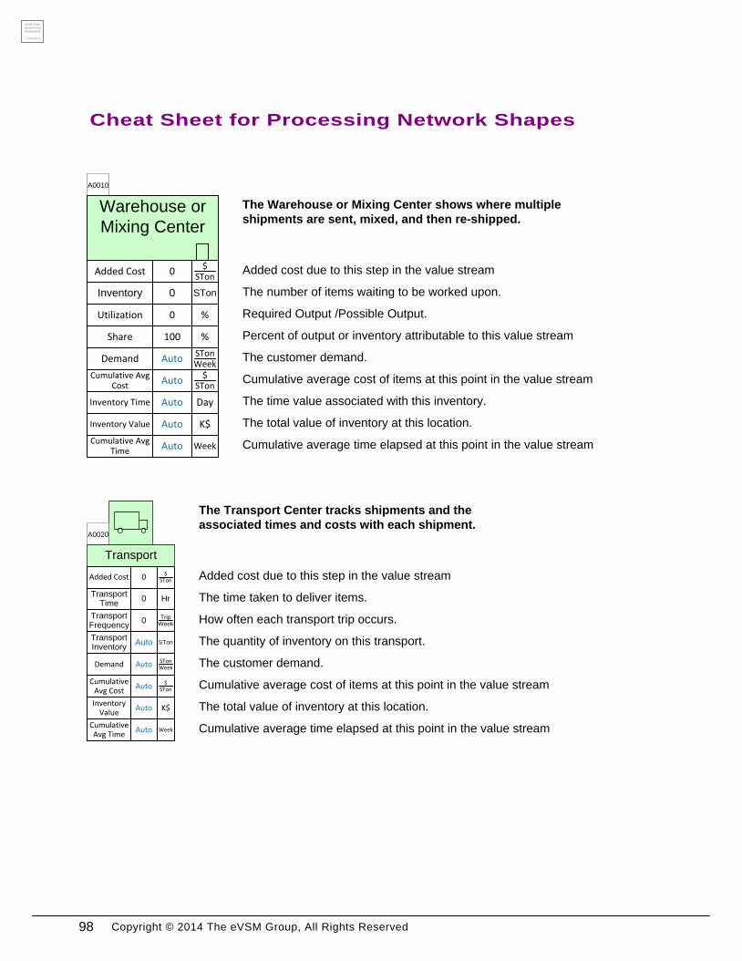
Copyright © 2014 The eVSM Group, All Rights Reserved
The Warehouse or Mixing Center shows where multiple
shipments are sent, mixed, and then re-shipped.Warehouse or
Mixing Center
A0010
DemandSTonWeek
Auto
Added Cost$
STon0
Cumulative Avg Cost
$STon
Auto
Inventory STon0
Inventory Time DayAuto
Inventory Value K$Auto
Cumulative Avg Time
WeekAuto
Utilization %0
Share %100
Transport
Demand STonWeekAuto
Added Cost $STon0
Cumulative Avg Cost
$STonAuto
Transport Inventory
STonAuto
Inventory Value
K$Auto
Cumulative Avg Time
WeekAuto
A0020
Transport Time
Hr0
Transport Frequency
TripWeek0
Added cost due to this step in the value stream
The number of items waiting to be worked upon.
Required Output /Possible Output.
The Transport Center tracks shipments and the
associated times and costs with each shipment.
Percent of output or inventory attributable to this value stream
The customer demand.
Cumulative average cost of items at this point in the value stream
The time value associated with this inventory.
The total value of inventory at this location.
Cumulative average time elapsed at this point in the value stream
Added cost due to this step in the value stream
The time taken to deliver items.
How often each transport trip occurs.
The quantity of inventory on this transport.
The customer demand.
Cumulative average cost of items at this point in the value stream
The total value of inventory at this location.
Cumulative average time elapsed at this point in the value stream
Cheat Sheet for Processing Network Shapes
eVSM Data
QuickProces
singNetwork
7.30.0026.3
98
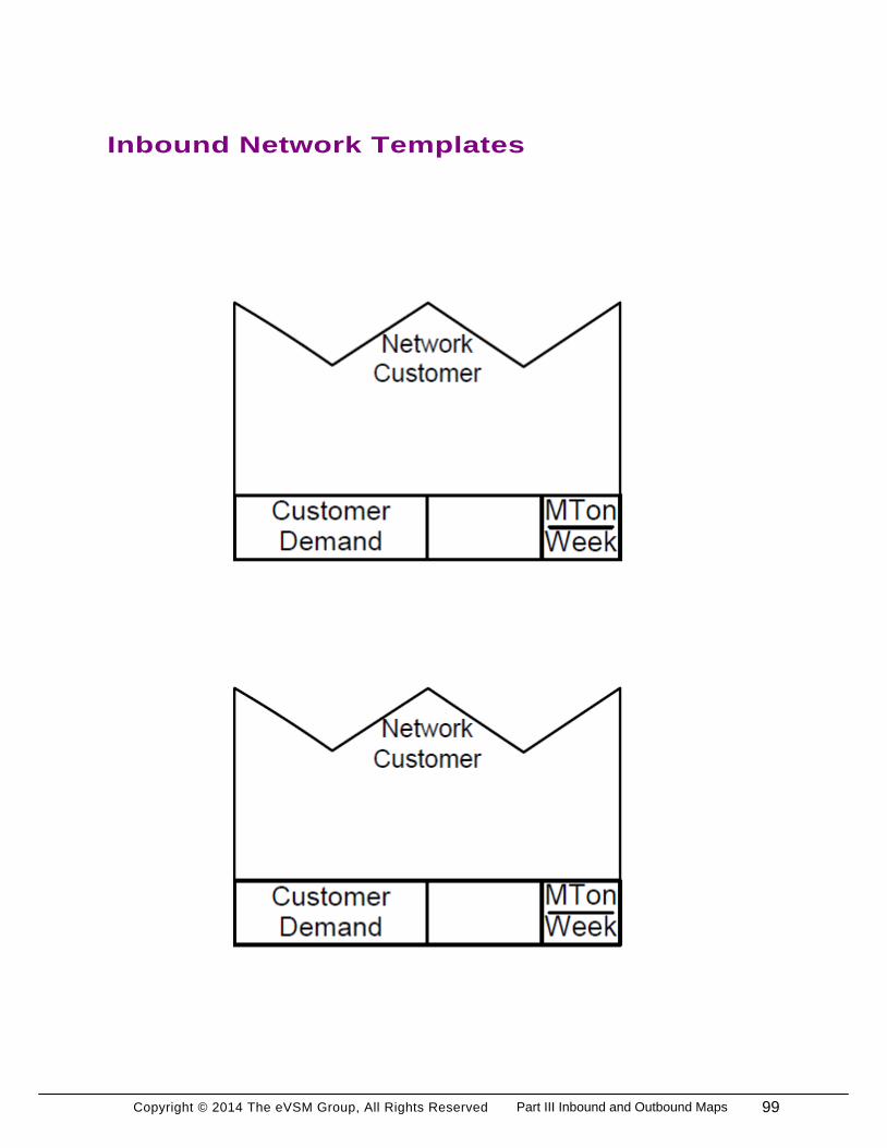
Copyright © 2014 The eVSM Group, All Rights Reserved
Inbound Network Templates
99Part III Inbound and Outbound Maps

Copyright © 2014 The eVSM Group, All Rights Reserved 100
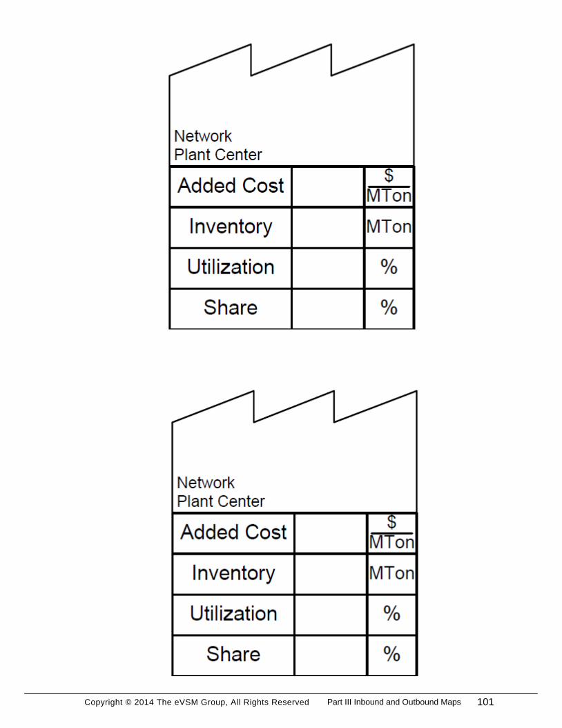
Copyright © 2014 The eVSM Group, All Rights Reserved 101Part III Inbound and Outbound Maps

Copyright © 2014 The eVSM Group, All Rights Reserved 102
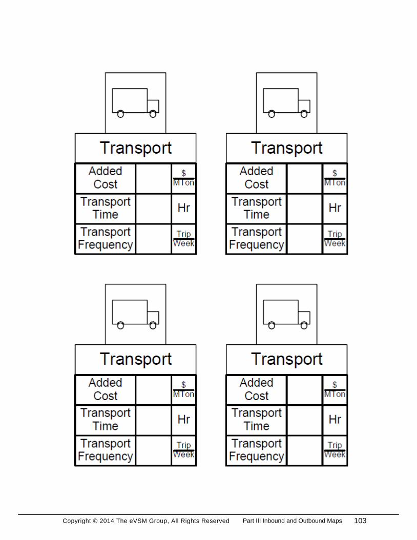
Copyright © 2014 The eVSM Group, All Rights Reserved 103Part III Inbound and Outbound Maps

Copyright © 2014 The eVSM Group, All Rights Reserved 104
Copyright © 2014 The eVSM Group, All Rights Reserved
eVSM Inbound Workshop
1. Insert the picture of the wall map using the Wall Map button in the eVSM toolbar.
2. Use the Open command in the eVSM toolbar to open the Quick Processing Network stencil.
3. Draw the map in eVSM.
4. Create sequence arrows and note that the sum of the DIW values coming into an activity
needs to add up to 100%.
5. Use the Auto Path button in the toolbar to assign path numbers.
6. Use the Auto Tag button to sequentially number the tags. (this affects charting)
7. Check the map and then Solve for the calculated fields.
105Part III Inbound and Outbound Maps
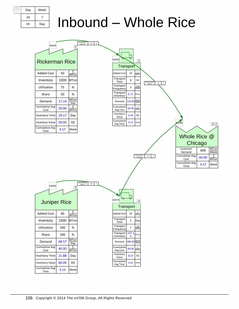
Copyright © 2014 The eVSM Group, All Rights Reserved
24
Day
Hr
7
Week
Day
Whole Rice @
Chicago
A0080
Customer Demand
MTonWeek
600
Cumulative Avg Cost
$MTon
60.00
Cumulative Avg Time
Week3.57
Rickerman Rice
A0040
DemandMTonDay
17.14
Added Cost$
MTon50
Cumulative Avg Cost
$MTon
50.00
Inventory MTon1000
Inventory Time Day29.17
Inventory Value K$50.00
Cumulative Avg Time
Week4.17
Utilization %75
Share %50
Juniper Rice
A0060
DemandMTonDay
68.57
Added Cost$
MTon40
Cumulative Avg Cost
$MTon
40.00
Inventory MTon1500
Inventory Time Day21.88
Inventory Value K$60.00
Cumulative Avg Time
Week3.13
Utilization %100
Share %100
Transport
Demand MTonWeek120.00
Added Cost $MTon10
Cumulative Avg Cost
$MTon60.00
Transport Inventory
MTon5.71
Inventory Value
K$0.34
Cumulative Avg Time
Week4.21
A0050
Transport Time
Hr8
Transport Frequency
TripWeek3
Transport
Demand MTonWeek480.00
Added Cost $MTon20
Cumulative Avg Cost
$MTon60.00
Transport Inventory
MTon137.1
4
Inventory Value
K$8.23
Cumulative Avg Time
Week3.41
A0070
Transport Time
Day2
Transport Frequency
TripWeek7
Downstream Input %
%100
Downstream Input %
%20
Downstream Input %
%100
Downstream Input %
%80
2
2
23
3
3
Inbound – Whole Rice
eVSM Data
QuickProces
singNetwork
7.30.0026.3
106
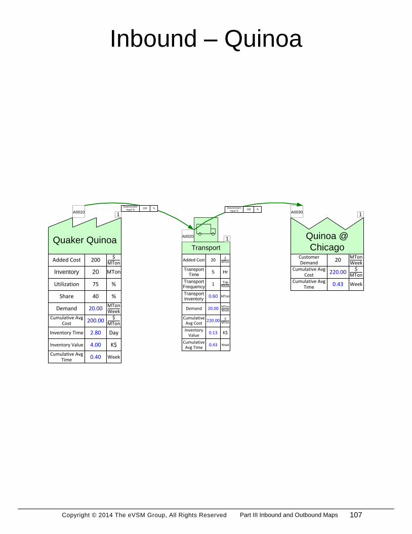
Copyright © 2014 The eVSM Group, All Rights Reserved
Quinoa @
Chicago
A0030
Customer Demand
MTonWeek
20
Cumulative Avg Cost
$MTon
220.00
Cumulative Avg Time
Week0.43
Quaker Quinoa
A0010
DemandMTonWeek
20.00
Added Cost$
MTon200
Cumulative Avg Cost
$MTon
200.00
Inventory MTon20
Inventory Time Day2.80
Inventory Value K$4.00
Cumulative Avg Time
Week0.40
Utilization %75
Share %40
Transport
Demand MTonWeek20.00
Added Cost $MTon20
Cumulative Avg Cost
$MTon220.00
Transport Inventory
MTon0.60
Inventory Value
K$0.13
Cumulative Avg Time
Week0.43
A0020
Transport Time
Hr5
Transport Frequency
TripWeek1
Downstream Input %
%100 Downstream Input %
%100
1
1
1
Inbound – Quinoa
107Part III Inbound and Outbound Maps
Copyright © 2014 The eVSM Group, All Rights Reserved
Enriched Grain - Outbound Chicago Rice Inc.
Exercise
With your group, read the information below and then:
1. Draw a wall value stream map for the product showing the supplier, warehouses,
transportation, and customers.
2. Show the data associated with the warehouses, transportation, and customers.
3. Calculate how many days of inventory you have at the plant and warehouses.
4. Calculate the demand at each warehouse and at the Chicago plant based on the customer
demand.
5. Identify useful summary metrics for the map.
6. Identify what charts would be useful to visualize the value stream and mark these up.
Background and Overview
Chicago Rice Inc. sells an enriched grain product which is made from a combination of rice and
quinoa. The outbound operations transport the enriched grain product to mixing centers and then
to the two customers, Maple Leaf Groceries and Jason Foods.
Value Stream Walk
To capture the current state value stream, you meet the logistics supervisor on Monday
afternoon. You learn that the outbound operations transport the enriched grain product to two
different warehouses. From there, trucks take the product to Maple Leaf Groceries and Jason
Foods. The grain product is shipped as bags each weighing 25 kilograms. Occasionally grain has
to be shipped from warehouse 1 to warehouse 2.
108
Copyright © 2014 The eVSM Group, All Rights Reserved
The logistics supervisor explains how the enriched grain product starts at our Chicago plant,
which has a utilization of 95%. Maple Leaf Groceries has a customer demand of 150 metric tons
(MTons) per week and is located close to Warehouse 1, which has a utilization of 75%. Chicago
Rice Inc. ships 70% of Maple Leaf Groceries’ demand to Warehouse 1 once a week with the
transportation taking 6 hours and costing an additional $20 per MTon. Warehouse 1 currently
holds 200 MTons and incurs an added cost of $15 per MTon. The remaining 30% of Maple Leaf
Groceries’ demand is sent in a shipment from Warehouse 2 to Warehouse 1 that occurs once per
week. The shipping takes 12 hours and adds a cost of $20 per MTon. Finally, Warehouse 1 ships
to Maple Leaf Groceries once per week, with each trip lasting 2 hours and adding a cost of $10
per MTon.
Jason Foods has a customer demand of 200 MTons per week. They receive their product from
Warehouse 2, which has a utilization of 97%. Warehouse 2 gets all of its supply directly from the
Chicago plant. The shipment from the Chicago plant to the warehouse takes 1 day and only
occurs once a week. Additional transportation costs are $10 per MTon. Warehouse 2 currently
holds 200 MTons which each have an added cost of $25 per MTon. Jason Foods then receives a
shipment from Warehouse 2 once per week. The transportation takes 1 day and adds a cost of $5
per MTon.
109Part III Inbound and Outbound Maps

Copyright © 2014 The eVSM Group, All Rights Reserved 110
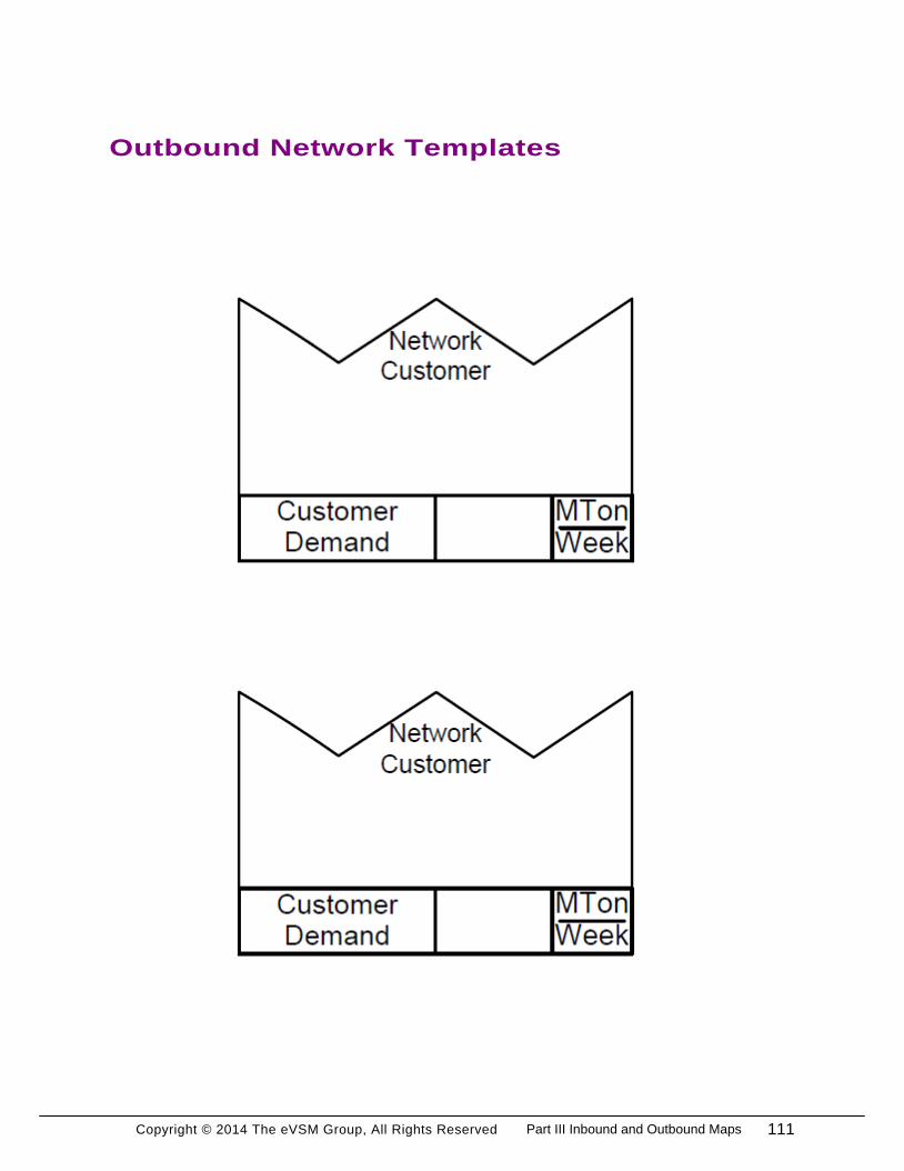
Copyright © 2014 The eVSM Group, All Rights Reserved
Outbound Network Templates
111Part III Inbound and Outbound Maps

Copyright © 2014 The eVSM Group, All Rights Reserved 112
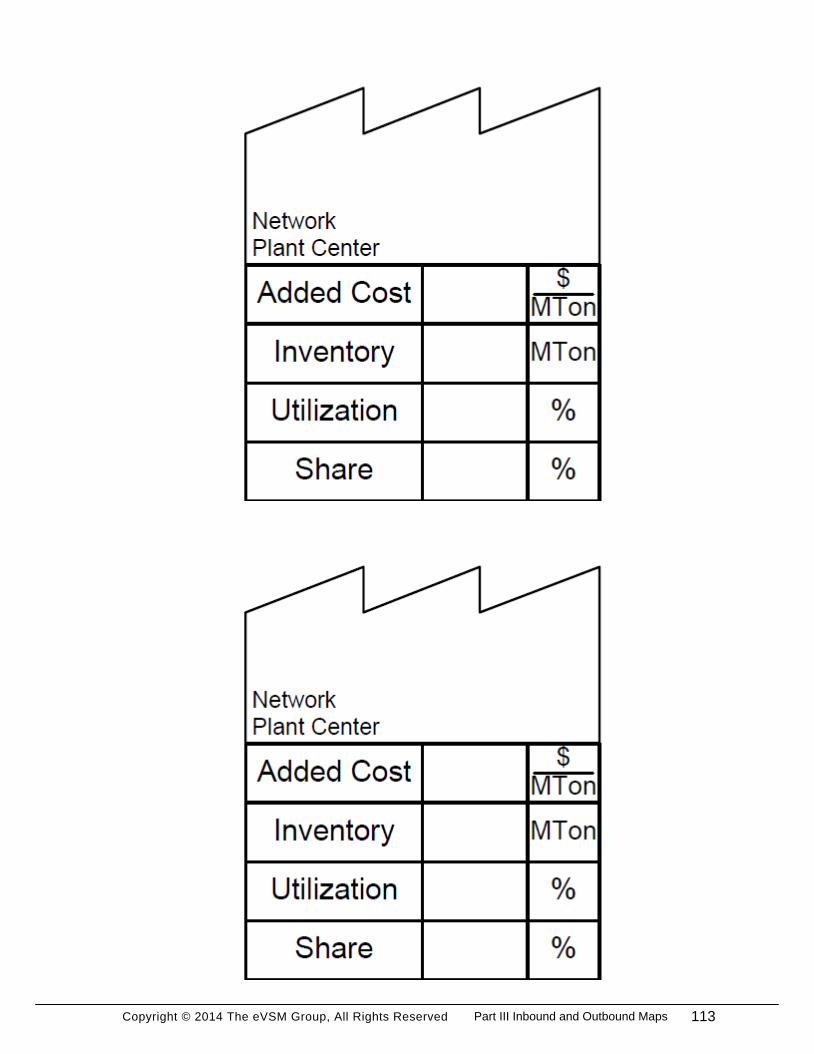
Copyright © 2014 The eVSM Group, All Rights Reserved 113Part III Inbound and Outbound Maps

Copyright © 2014 The eVSM Group, All Rights Reserved 114
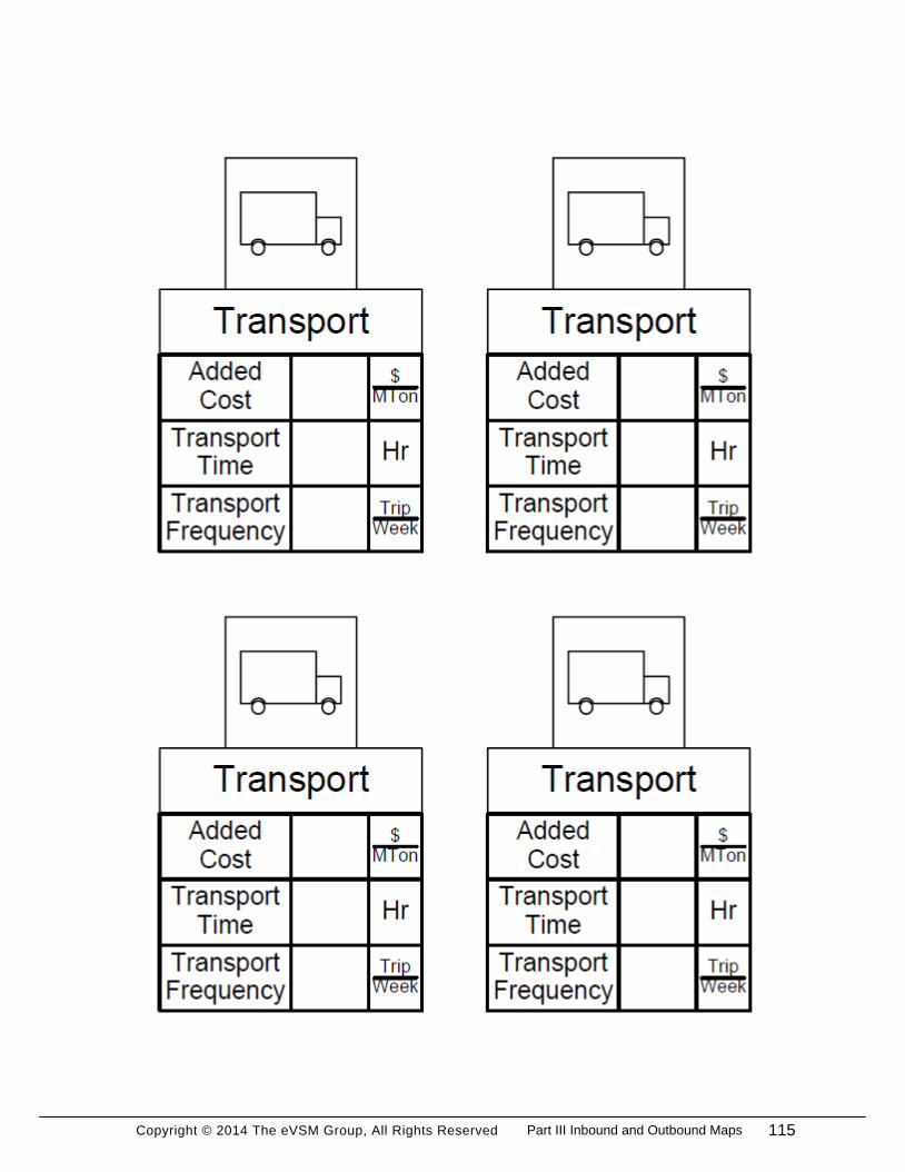
Copyright © 2014 The eVSM Group, All Rights Reserved 115Part III Inbound and Outbound Maps

Copyright © 2014 The eVSM Group, All Rights Reserved 116
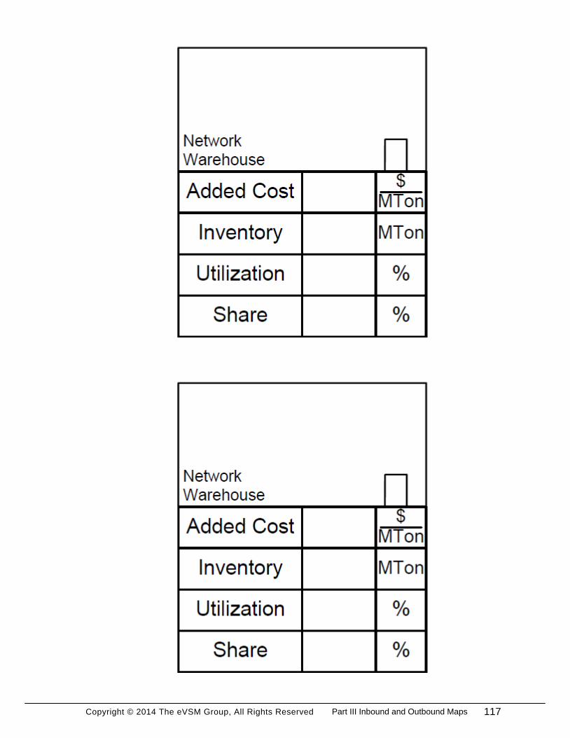
Copyright © 2014 The eVSM Group, All Rights Reserved 117Part III Inbound and Outbound Maps

Copyright © 2014 The eVSM Group, All Rights Reserved
eVSM Data
QuickProces
sing
7.30.0111.1
118
Copyright © 2014 The eVSM Group, All Rights Reserved
eVSM Outbound Workshop
1. Insert the picture of the wall map using the Wall Map button in the toolbar.
2. Use the Open command in the eVSM toolbar to open the Quick Processing Network stencil.
3. Draw the map in eVSM.
4. Create sequence arrows and note that the sum of the DIW values coming into an activity
needs to add up to 100%.
5. Use the Auto Path button in the toolbar to assign path numbers.
6. Use the Auto Tag button to sequentially number the tags. (this affects charting)
7. Check the map and then Solve for the calculated fields.
119Part III Inbound and Outbound Maps
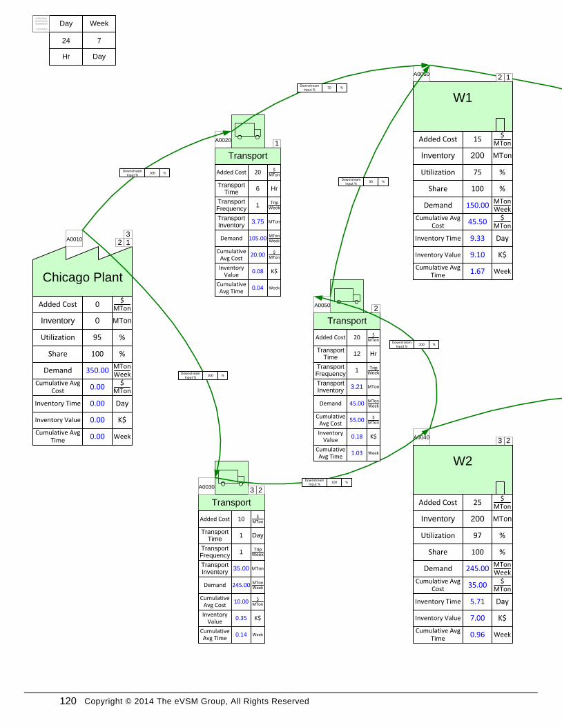
Copyright © 2014 The eVSM Group, All Rights Reserved
24
Day
Hr
7
Week
Day
Chicago Plant
A0010
DemandMTonWeek
350.00
Added Cost$
MTon0
Cumulative Avg Cost
$MTon
0.00
Inventory MTon0
Inventory Time Day0.00
Utilization %95
Share %100
W1
A0060
DemandMTonWeek
150.00
Added Cost$
MTon15
Cumulative Avg Cost
$MTon
45.50
Inventory MTon200
Inventory Time Day9.33
Utilization %75
Share %100
W2
A0040
DemandMTonWeek
245.00
Added Cost$
MTon25
Cumulative Avg Cost
$MTon
35.00
Inventory MTon200
Inventory Time Day5.71
Utilization %97
Share %100
Transport
Demand MTonWeek105.00
Added Cost $MTon20
Cumulative Avg Cost
$MTon20.00
Transport Inventory
MTon3.75
A0020
Transport Time
Hr6
Transport Frequency
TripWeek1
Transport
Demand MTonWeek245.00
Added Cost $MTon10
Cumulative Avg Cost
$MTon10.00
Transport Inventory
MTon35.00
A0030
Transport Time
Day1
Transport Frequency
TripWeek1
Transport
Demand MTonWeek45.00
Added Cost $MTon20
Cumulative Avg Cost
$MTon55.00
Transport Inventory
MTon3.21
A0050
Transport Time
Hr12
Transport Frequency
TripWeek1
Downstream Input %
%100
Downstream Input %
%70
Downstream Input %
%100
Downstream Input %
%100
Downstream Input %
%30
Downstream Input %
%100
Inventory Value K$0.00
Cumulative Avg Time
Week0.00
Inventory Value K$9.10
Cumulative Avg Time
Week1.67
Inventory Value K$7.00
Cumulative Avg Time
Week0.96
Inventory Value
K$0.08
Cumulative Avg Time
Week0.04
Inventory Value
K$0.35
Cumulative Avg Time
Week0.14
Inventory Value
K$0.18
Cumulative Avg Time
Week1.03
123
1
12
23
23
2
eVSM Data
QuickProces
singNetwork
7.30.0026.3
120
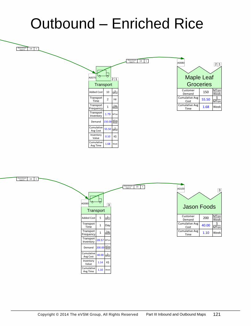
Copyright © 2014 The eVSM Group, All Rights Reserved
Outbound – Enriched Rice
Maple Leaf
Groceries
A0080
Customer Demand
MTonWeek
150
Cumulative Avg Cost
$MTon
55.50
Jason Foods
A0100
Customer Demand
MTonWeek
200
Cumulative Avg Cost
$MTon
40.00
Transport
Demand MTonWeek200.00
Added Cost $MTon5
Cumulative Avg Cost
$MTon40.00
Transport Inventory
MTon28.57
A0090
Transport Time
Day1
Transport Frequency
TripWeek1
Transport
Demand MTonWeek150.00
Added Cost $MTon10
Cumulative Avg Cost
$MTon55.50
Transport Inventory
MTon1.79
A0070
Transport Time
Hr2
Transport Frequency
TripWeek1
Downstream Input %
%100
Downstream Input %
%100
Downstream Input %
%100
Downstream Input %
%100
Cumulative Avg Time
Week1.68
Cumulative Avg Time
Week1.10
Inventory Value
K$1.14
Cumulative Avg Time
Week1.10
Inventory Value
K$0.10
Cumulative Avg Time
Week1.68
12
12
3
3
121Part III Inbound and Outbound Maps

Copyright © 2014 The eVSM Group, All Rights Reserved 122

Copyright © 2014 The eVSM Group, All Rights Reserved
Part IV: Linking Maps Together
123Part IV Linking Maps Together
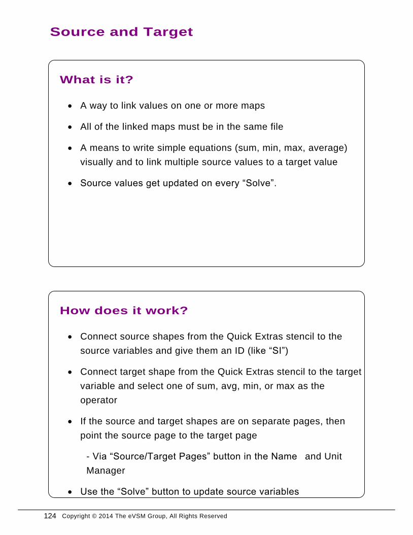
Copyright © 2014 The eVSM Group, All Rights Reserved
· A way to link values on one or more maps
· All of the linked maps must be in the same file
· A means to write simple equations (sum, min, max, average)
visually and to link multiple source values to a target value
· Source values get updated on every “Solve”.
What is it?
· Connect source shapes from the Quick Extras stencil to the
source variables and give them an ID (like “SI”)
· Connect target shape from the Quick Extras stencil to the target
variable and select one of sum, avg, min, or max as the
operator
· If the source and target shapes are on separate pages, then
point the source page to the target page
- Via “Source/Target Pages” button in the Name and Unit
Manager
· Use the “Solve” button to update source variables
How does it work?
Source and Target
124
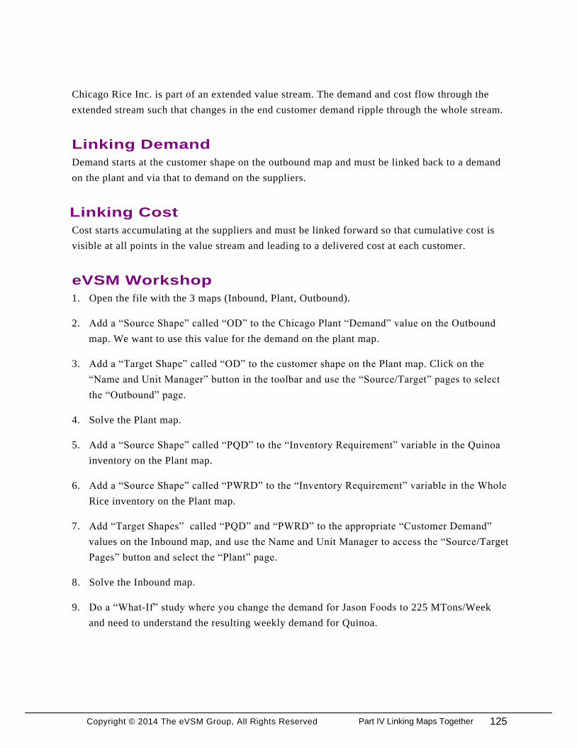
Copyright © 2014 The eVSM Group, All Rights Reserved
Linking Demand
Chicago Rice Inc. is part of an extended value stream. The demand and cost flow through the
extended stream such that changes in the end customer demand ripple through the whole stream.
Linking Cost
Demand starts at the customer shape on the outbound map and must be linked back to a demand
on the plant and via that to demand on the suppliers.
Cost starts accumulating at the suppliers and must be linked forward so that cumulative cost is
visible at all points in the value stream and leading to a delivered cost at each customer.
eVSM Workshop
1. Open the file with the 3 maps (Inbound, Plant, Outbound).
2. Add a “Source Shape” called “OD” to the Chicago Plant “Demand” value on the Outbound
map. We want to use this value for the demand on the plant map.
3. Add a “Target Shape” called “OD” to the customer shape on the Plant map. Click on the
“Name and Unit Manager” button in the toolbar and use the “Source/Target” pages to select
the “Outbound” page.
4. Solve the Plant map.
5. Add a “Source Shape” called “PQD” to the “Inventory Requirement” variable in the Quinoa
inventory on the Plant map.
6. Add a “Source Shape” called “PWRD” to the “Inventory Requirement” variable in the Whole
Rice inventory on the Plant map.
7. Add “Target Shapes” called “PQD” and “PWRD” to the appropriate “Customer Demand”
values on the Inbound map, and use the Name and Unit Manager to access the “Source/Target
Pages” button and select the “Plant” page.
8. Solve the Inbound map.
9. Do a “What-If” study where you change the demand for Jason Foods to 225 MTons/Week
and need to understand the resulting weekly demand for Quinoa.
125Part IV Linking Maps Together

Copyright © 2014 The eVSM Group, All Rights Reserved 126

Copyright © 2014 The eVSM Group, All Rights Reserved
eVSM Extras
127eVSM Extras
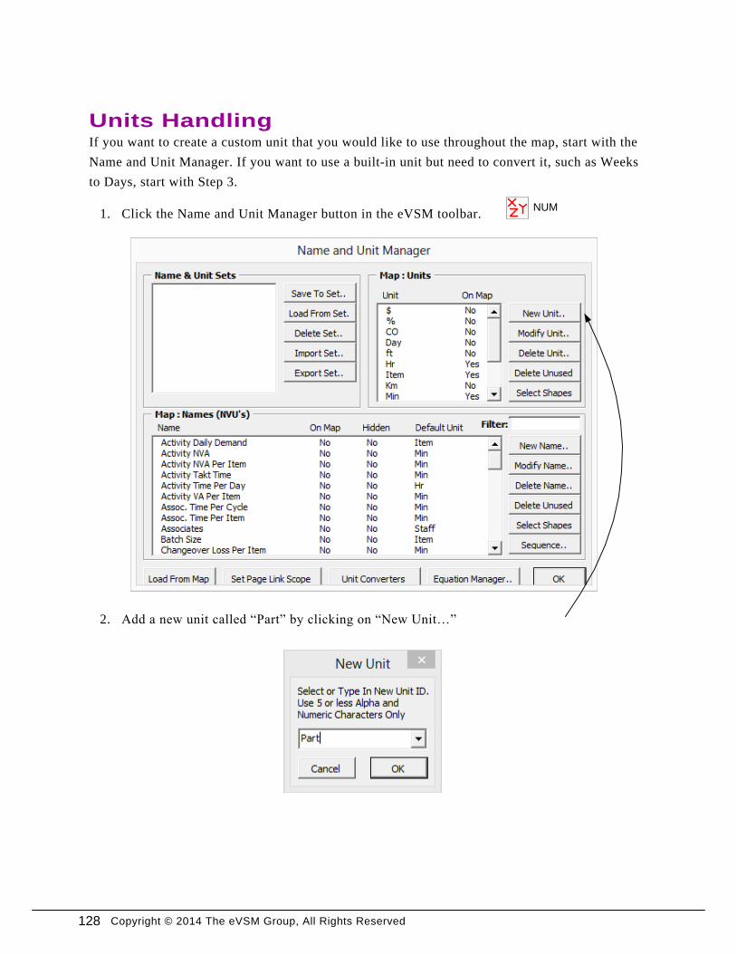
Copyright © 2014 The eVSM Group, All Rights Reserved
If you want to create a custom unit that you would like to use throughout the map, start with the
Name and Unit Manager. If you want to use a built-in unit but need to convert it, such as Weeks
to Days, start with Step 3.
1. Click the Name and Unit Manager button in the eVSM toolbar.
Units Handling
NUM
2. Add a new unit called “Part” by clicking on “New Unit…”
128
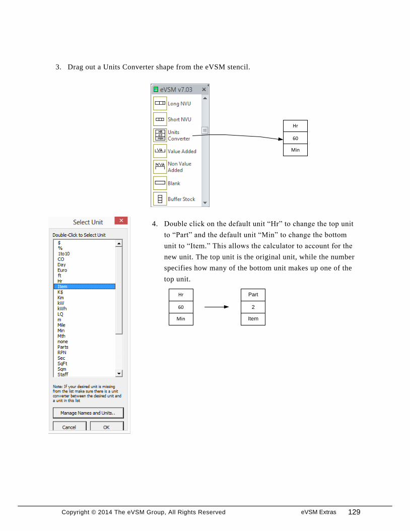
Copyright © 2014 The eVSM Group, All Rights Reserved
60
Hr
Min
2
Part
Item
60
Hr
Min
3. Drag out a Units Converter shape from the eVSM stencil.
4. Double click on the default unit “Hr” to change the top unit
to “Part” and the default unit “Min” to change the bottom
unit to “Item.” This allows the calculator to account for the
new unit. The top unit is the original unit, while the number
specifies how many of the bottom unit makes up one of the
top unit.
129eVSM Extras
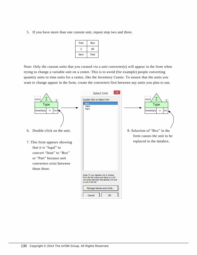
Copyright © 2014 The eVSM Group, All Rights Reserved
5. If you have more than one custom unit, repeat step two and three.
2
Part
Item
60
Box
Part
1
Inventory Itemxx
A0010
Type
1
Inventory Boxxx
A0020
Type
6. Double-click on the unit.
Note: Only the custom units that you created via a unit converter(s) will appear in the form when
trying to change a variable unit on a center. This is to avoid (for example) people converting
quantity units to time units for a center, like the Inventory Center. To ensure that the units you
want to change appear in the form, create the converters first between any units you plan to use.
7. This form appears showing
that it is “legal” to
convert “Item” to “Box”
or “Part” because unit
converters exist between
these three.
8. Selection of “Box” in the
form causes the unit to be
replaced in the databox.
130
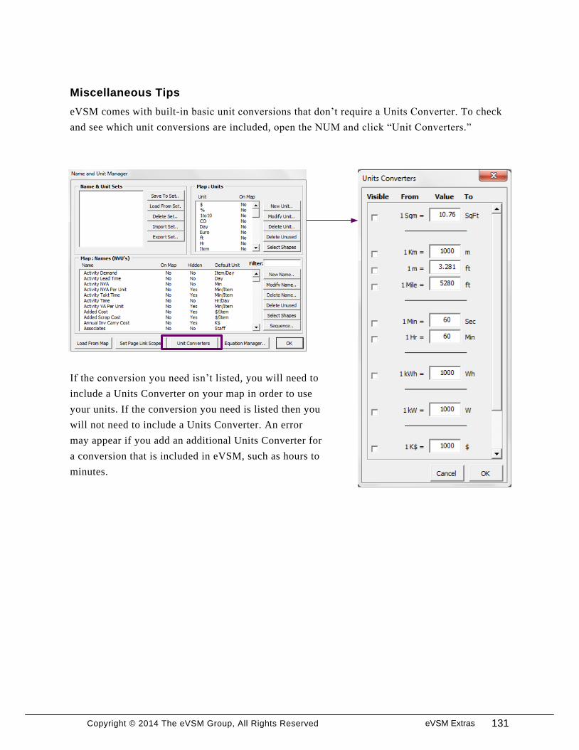
Copyright © 2014 The eVSM Group, All Rights Reserved
Miscellaneous Tips
eVSM comes with built-in basic unit conversions that don’t require a Units Converter. To check
and see which unit conversions are included, open the NUM and click “Unit Converters.”
If the conversion you need isn’t listed, you will need to
include a Units Converter on your map in order to use
your units. If the conversion you need is listed then you
will not need to include a Units Converter. An error
may appear if you add an additional Units Converter for
a conversion that is included in eVSM, such as hours to
minutes.
131eVSM Extras
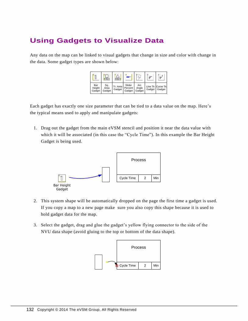
Copyright © 2014 The eVSM Group, All Rights Reserved
Any data on the map can be linked to visual gadgets that change in size and color with change in
the data. Some gadget types are shown below:
Sq. Area
Gadget
Tr. Area Gadget
Slider Percent Gadget
Arc Angle
Gadget
Line Tk Gadget
Bar Height Gadget
Curve Tk Gadget
Each gadget has exactly one size parameter that can be tied to a data value on the map. Here’s
the typical means used to apply and manipulate gadgets:
1. Drag out the gadget from the main eVSM stencil and position it near the data value with
which it will be associated (in this case the “Cycle Time”). In this example the Bar Height
Gadget is being used.
Bar Height Gadget
Using Gadgets to Visualize Data
Process
Cycle Time Min2
2. This system shape will be automatically dropped on the page the first time a gadget is used.
If you copy a map to a new page make sure you also copy this shape because it is used to
hold gadget data for the map.
3. Select the gadget, drag and glue the gadget’s yellow flying connector to the side of the
NVU data shape (avoid gluing to the top or bottom of the data shape).
Process
Cycle Time Min2
132
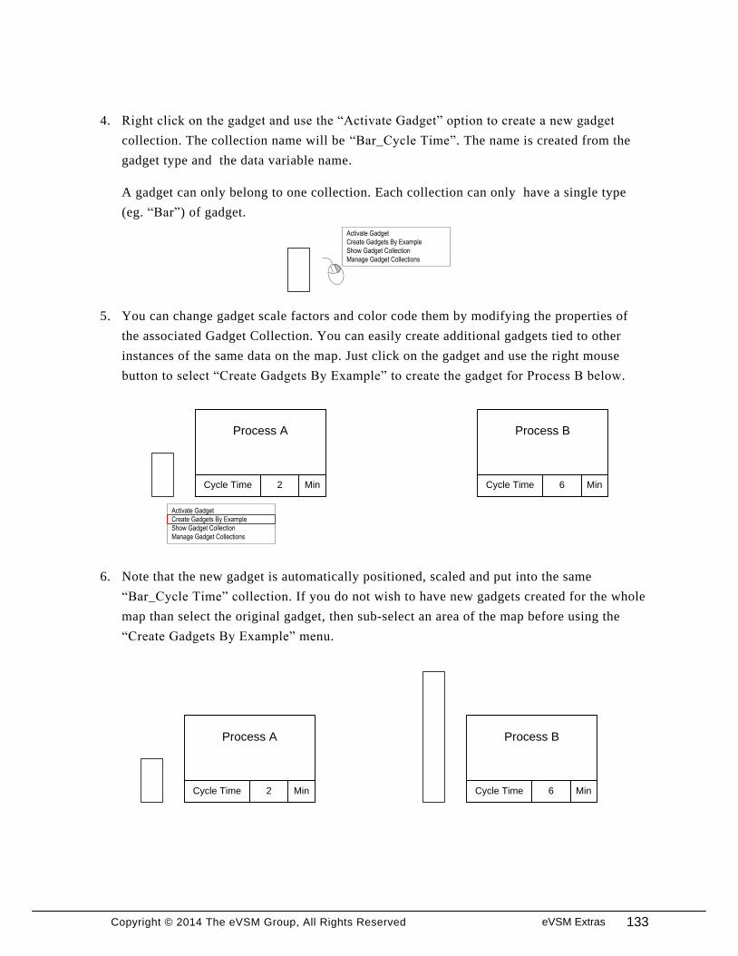
Copyright © 2014 The eVSM Group, All Rights Reserved
4. Right click on the gadget and use the “Activate Gadget” option to create a new gadget
collection. The collection name will be “Bar_Cycle Time”. The name is created from the
gadget type and the data variable name.
A gadget can only belong to one collection. Each collection can only have a single type
(eg. “Bar”) of gadget.
Activate Gadget
Create Gadgets By Example
Show Gadget Collection
Manage Gadget Collections
5. You can change gadget scale factors and color code them by modifying the properties of
the associated Gadget Collection. You can easily create additional gadgets tied to other
instances of the same data on the map. Just click on the gadget and use the right mouse
button to select “Create Gadgets By Example” to create the gadget for Process B below.
Process A
Cycle Time Min2
6. Note that the new gadget is automatically positioned, scaled and put into the same
“Bar_Cycle Time” collection. If you do not wish to have new gadgets created for the whole
map than select the original gadget, then sub-select an area of the map before using the
“Create Gadgets By Example” menu.
Process A
Cycle Time Min2
Process B
Cycle Time Min6
Activate Gadget
Create Gadgets By Example
Show Gadget Collection
Manage Gadget Collections
Process B
Cycle Time Min6
133eVSM Extras
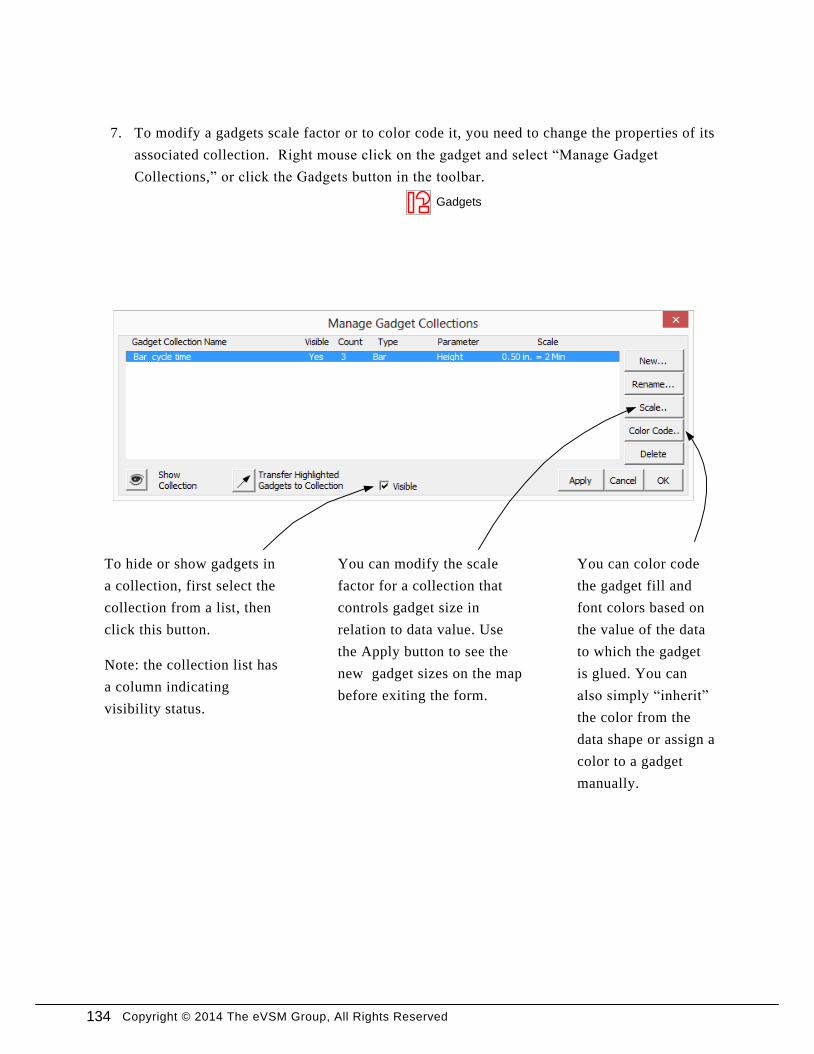
Copyright © 2014 The eVSM Group, All Rights Reserved
7. To modify a gadgets scale factor or to color code it, you need to change the properties of its
associated collection. Right mouse click on the gadget and select “Manage Gadget
Collections,” or click the Gadgets button in the toolbar.
Gadgets
You can color code
the gadget fill and
font colors based on
the value of the data
to which the gadget
is glued. You can
also simply “inherit”
the color from the
data shape or assign a
color to a gadget
manually.
You can modify the scale
factor for a collection that
controls gadget size in
relation to data value. Use
the Apply button to see the
new gadget sizes on the map
before exiting the form.
To hide or show gadgets in
a collection, first select the
collection from a list, then
click this button.
Note: the collection list has
a column indicating
visibility status.
134
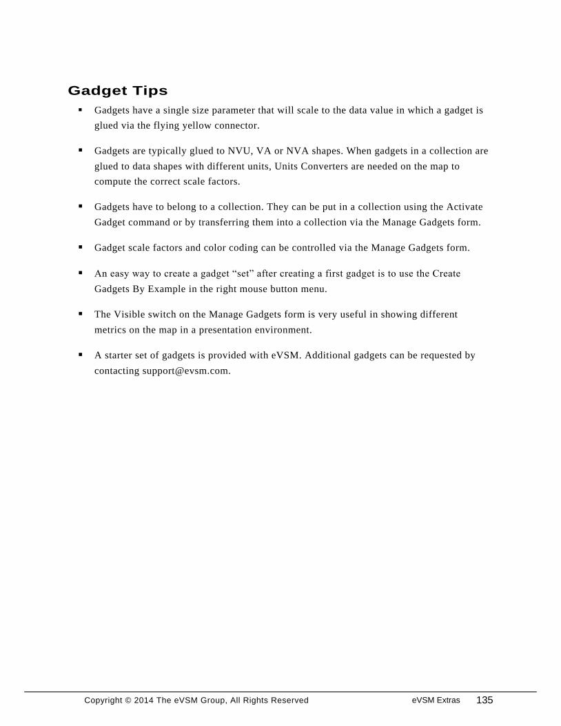
Copyright © 2014 The eVSM Group, All Rights Reserved
§ Gadgets have a single size parameter that will scale to the data value in which a gadget is
glued via the flying yellow connector.
§ Gadgets are typically glued to NVU, VA or NVA shapes. When gadgets in a collection are
glued to data shapes with different units, Units Converters are needed on the map to
compute the correct scale factors.
§ Gadgets have to belong to a collection. They can be put in a collection using the Activate
Gadget command or by transferring them into a collection via the Manage Gadgets form.
§ Gadget scale factors and color coding can be controlled via the Manage Gadgets form.
§ An easy way to create a gadget “set” after creating a first gadget is to use the Create
Gadgets By Example in the right mouse button menu.
§ The Visible switch on the Manage Gadgets form is very useful in showing different
metrics on the map in a presentation environment.
§ A starter set of gadgets is provided with eVSM. Additional gadgets can be requested by
contacting [email protected].
Gadget Tips
135eVSM Extras
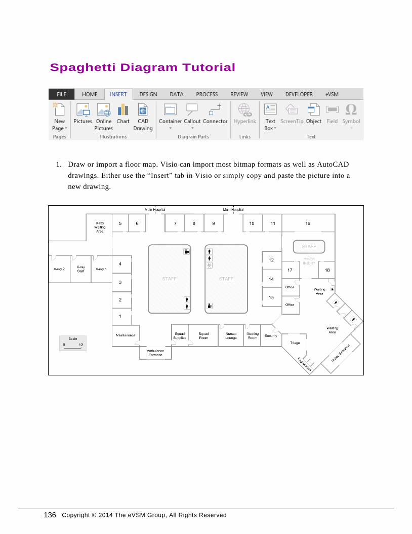
Copyright © 2014 The eVSM Group, All Rights Reserved
1. Draw or import a floor map. Visio can import most bitmap formats as well as AutoCAD
drawings. Either use the “Insert” tab in Visio or simply copy and paste the picture into a
new drawing.
Spaghetti Diagram Tutorial
136
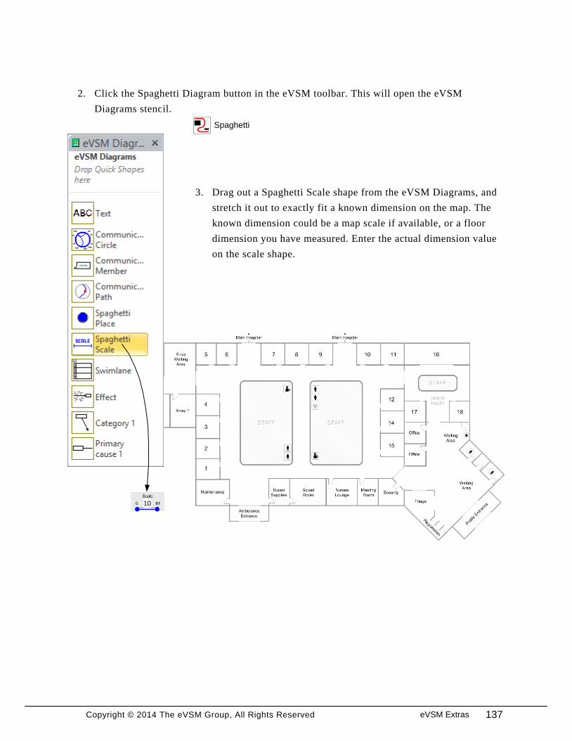
Copyright © 2014 The eVSM Group, All Rights Reserved
2. Click the Spaghetti Diagram button in the eVSM toolbar. This will open the eVSM
Diagrams stencil.
Spaghetti
3. Drag out a Spaghetti Scale shape from the eVSM Diagrams, and
stretch it out to exactly fit a known dimension on the map. The
known dimension could be a map scale if available, or a floor
dimension you have measured. Enter the actual dimension value
on the scale shape.
10
137eVSM Extras
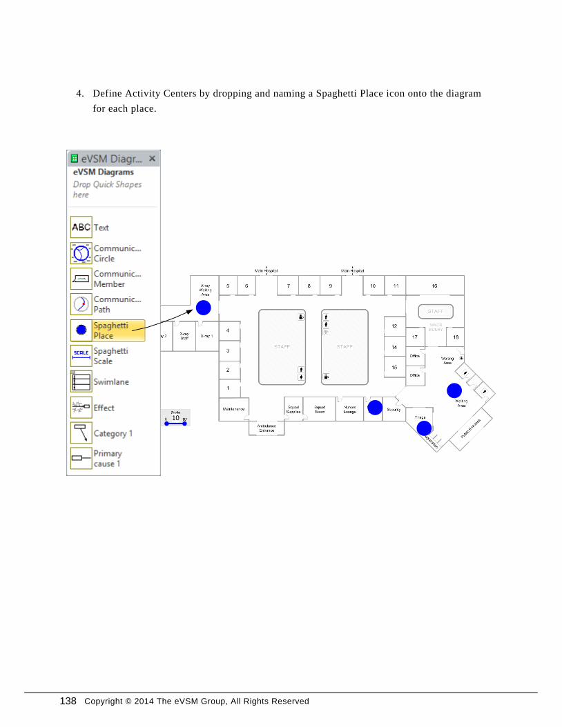
Copyright © 2014 The eVSM Group, All Rights Reserved
4. Define Activity Centers by dropping and naming a Spaghetti Place icon onto the diagram
for each place.
10
138
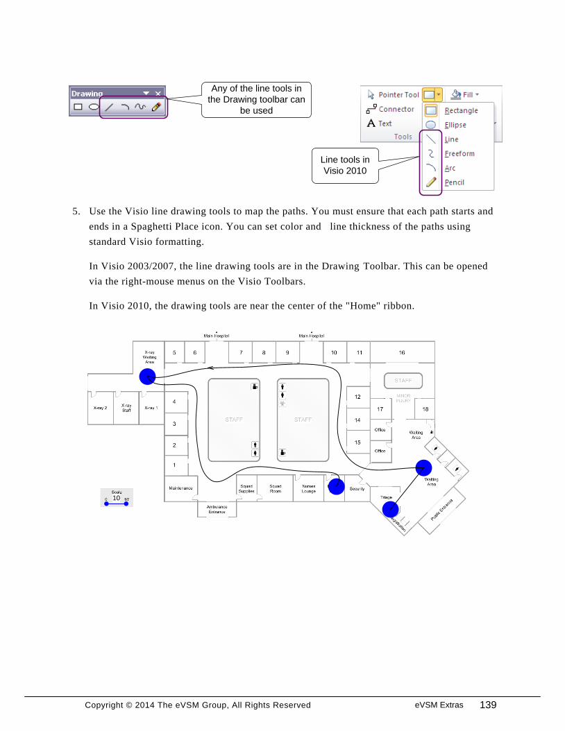
Copyright © 2014 The eVSM Group, All Rights Reserved
5. Use the Visio line drawing tools to map the paths. You must ensure that each path starts and
ends in a Spaghetti Place icon. You can set color and line thickness of the paths using
standard Visio formatting.
In Visio 2003/2007, the line drawing tools are in the Drawing Toolbar. This can be opened
via the right-mouse menus on the Visio Toolbars.
In Visio 2010, the drawing tools are near the center of the "Home" ribbon.
Any of the line tools in
the Drawing toolbar can
be used
Line tools in
Visio 2010
10
139eVSM Extras
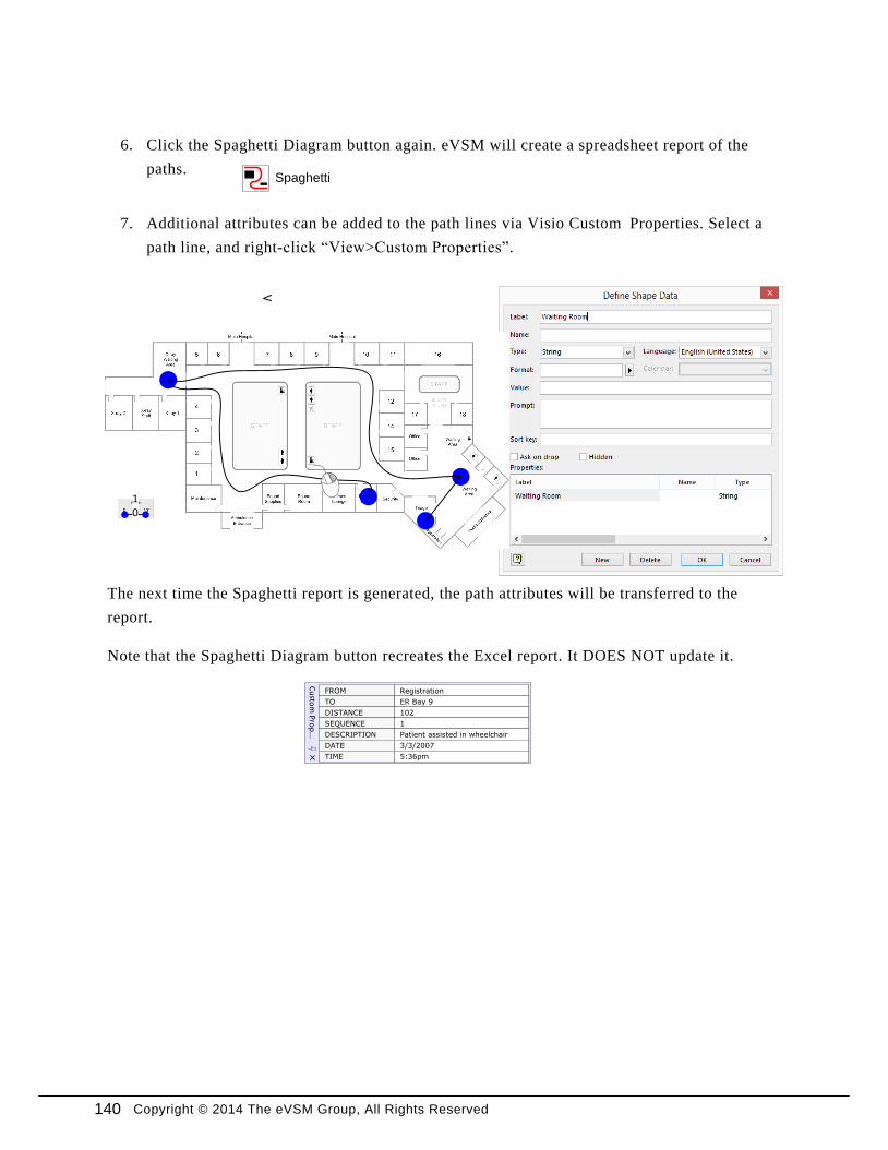
Copyright © 2014 The eVSM Group, All Rights Reserved
6. Click the Spaghetti Diagram button again. eVSM will create a spreadsheet report of the
paths.
7. Additional attributes can be added to the path lines via Visio Custom Properties. Select a
path line, and right-click “View>Custom Properties”.
The next time the Spaghetti report is generated, the path attributes will be transferred to the
report.
Note that the Spaghetti Diagram button recreates the Excel report. It DOES NOT update it.
Spaghetti
10
FROM Registration
ER Bay 9TO
DISTANCE 102
SEQUENCE 1
DESCRIPTION Patient assisted in wheelchair
DATE 3/3/2007
TIME 5:36pm
Cu
stom
Pro
p...
140

Copyright © 2014 The eVSM Group, All Rights Reserved 141eVSM Extras

Copyright © 2014 The eVSM Group, All Rights Reserved
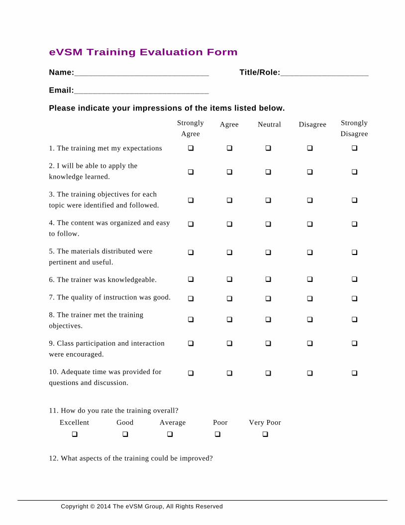
Copyright © 2014 The eVSM Group, All Rights Reserved
eVSM Training Evaluation Form
Name:_____________________________ Title/Role:___________________
Email:_____________________________
Please indicate your impressions of the items listed below.
Strongly
Agree
Agree Neutral Disagree Strongly
Disagree
1. The training met my expectations
2. I will be able to apply the
knowledge learned.
3. The training objectives for each
topic were identified and followed.
4. The content was organized and easy
to follow.
5. The materials distributed were
pertinent and useful.
6. The trainer was knowledgeable.
7. The quality of instruction was good.
8. The trainer met the training
objectives.
9. Class participation and interaction
were encouraged.
10. Adequate time was provided for
questions and discussion.
11. How do you rate the training overall?
q q q q q
q q q q q
q q q q q
q q q q q
q q q q q
q q q q q
q q q q q
q q q q q
q q q q q
q q q q q
q q q q q
Excellent Good Average Poor Very Poor
12. What aspects of the training could be improved?
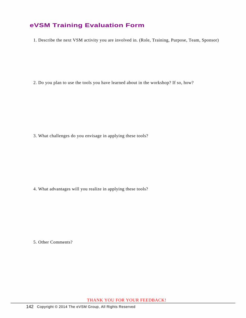
Copyright © 2014 The eVSM Group, All Rights Reserved
eVSM Training Evaluation Form
THANK YOU FOR YOUR FEEDBACK!
1. Describe the next VSM activity you are involved in. (Role, Training, Purpose, Team, Sponsor)
2. Do you plan to use the tools you have learned about in the workshop? If so, how?
3. What challenges do you envisage in applying these tools?
4. What advantages will you realize in applying these tools?
5. Other Comments?
142


![Volume 7 - Inventory - SAP Business One Hana On Cloud ... · Saks Itžm Purchase Item Inventory Non Value In ventary Item TORY Serizl and Batch Numbers M e Item None C] Do Not Apply](https://img.pdfslide.net/doc/110x75/5c936dc009d3f21a398c2368/volume-7-inventory-sap-business-one-hana-on-cloud-saks-itzm-purchase.jpg)