exact computation of optimal inventory policies over an unbounded

MATHEMATICS OF OPERATIONS RESEARCH Vol. 16, No. 3, August 1991 Printed m U.S.A.

EXACT COMPUTATION OF OPTIMAL INVENTORY POLICIES OVER AN UNBOUNDED HORIZON*

REFAEL HASSIN AND NIMROD MEGIDDO

An inventory scheduling model with forbidden time intervals is analyzed. The objective is to minimize the long-term average cost per time unit. Unlike most of the literature on inventory theory, no restrictive assumptions are made a priori about the nature of optimal solutions. Rather it is proved that optimal policies exist, and that some of them are cyclic with cycles of a particular structure. It is then shown that such optimal policies can be computed and an algorithm is given.

1. Introduction. In the classical Economic Order Quantity (EOQ) model one seeks a policy of inventory scheduling so as to minimize the long-term average cost per time unit. Inventory is depleted at a known constant rate R and can be replenished instantaneously at any time. There is a fixed cost of Cf per order, and the inventory holding cost is proportional to the amount of time and the amount of commodity held in stock: C, per time unit for each unit of commodity. Given that an order is placed at time t , it is straightforward to find the time of the next order t + x so as to minimize the average cost per time unit over [ t , t + x):

This turns out to be x* = J2C,/02C,/0. A nice feature of this model is that the policy of ordering every x*. time units is optimal in the following strong sense: it minimizes the limsup (as T tends to infinity) of the average cost per unit over the interval [0, T ) among all possible schedules over an unbounded horizon.

There is a vast literature on inventory and production models generalizing the EOQ in numerous directions. Usually the models are stated precisely but the policies found are only approximately optimal or optimal only within a restricted class of policies which is more amenable for analysis (see, for example, [2], [3], [41, [S], [6], [8]). For example, many authors simply assume that there exists a cyclic optimal policy and set out to find a best cyclic one. Another common assumption is that orders are placed (or production is resumed) only when the inventory level reaches zero. In many cases such an assumption turns out to be wrong. There have been cases where authors made restrictive assumptions that were hard to justify and several mathematical pitfalls have been pointed out [I], [71, [9].

When we started the work presented in this paper our goal was to carry out an exact analysis of a model more general than the classical EOQ, where it is not a priori clear whether optimal policies exist, or whether optimality of a given policy can be decided. We were quite surprised to discover the complexities involved in the simple model we were looking at. It turned out, however, to be decidable in a nontrivial way.

*Received November 2, 1988: revised November 9, 1989. AMS 1980 subject ctuss~cation. Primary: 90B05. Secondary: 90A16. lAOR 1973 subject classification. Main: Inventory. Cross references: optimization. OR/MS Index 1978 subject classificution. Primary: 346 Inventory/production/policies. Key words. Optimal inventory policies, infinite horizon, deterministic.

0364-765X/91/1603/0534/$01.25 Copyright G 1991, The Institute of Mana~ement Sciences/Ope.rat~ons Research Society of Amcrica

EXACT COMPUTATION OF OPTIMAL INVENTORY POLICIES 535

We consider a deterministic inventory problem over an unbounded horizon. The objective is to minimize cost. More precisely, setup costs and inventory holding costs are averaged over time and a policy is evaluated by either the Iiminf or the limsup (as T tends to infinity) of the average total cost per time unit incurred during the first T time units. We actually show that there exist policies where this average tends to a limit which is equal to the infimum of the liminfs over all policies and hence also to the infimum of the Iimsups.

A precise statement of the problem is as follows. PROBLEM 1.1. Given a real number a, 0 < a < 1, a commodity can be ordered at

any time except during intervals of the form (I, I + a) , where I is an integer. There is a fixed positive cost associated with every order and there is an inventory holding cost proportional to the amount of time and the amount of inventory. Inventory is depleted at a constant rate, which is called the demand rate. The order is filled instantaneously. A feasible solution is a policy consisting of feasible times of orders and amounts such that the demand is always satisfied. A policy E is called optimal if the limsup of the average cost per time over the interval [O, T), denoted Z(B), is minimum among all policies.

2. Preliminaries. The existence of feasible policies is obvious but we can actually prove:

PROPOSITION 2.1. There exist optimal policies.

PROOF. Suppose c* is the infimum of E(E) taken over all the feasible policies 8. Thus, for any k > 0 there exists a policy Bk such that for every sufficiently large T, the average cost per time unit of Bk over the interval [O, T) is less than c" + l/k. The idea of the proof is to generate a policy B which uses portions of the policies Bk successively, for k = 1,2, . . . . We construct below a sequence of positive integers (7,) which determines an optimal policy Z as follows. Over the interval [O, r,), the policy B works essentially like E1 over the same interval, except that if the inventory level at r1 is positive, then the sizes of one or more orders before T, are reduced to obtain a new feasible solution where the inventory level at r, is zero. Denote a; = C ~ = , r j . Over the interval [a,-,, uk), E is essentially the same as Bk during the interval [O, 7,). Without loss of generality, assume that for every k the average cost of Bk over the interval [0, T) is bounded over all values of T. Now, there exists r , such that for any T 2 T,, the average cost over [O, T) of running 8' over [O, T,), and then the first T - r, time units of E2 over [ r l , T ) , is less than c* + 2. Inductively, suppose we have determined T, , . . . , rk -, , and the policy B has already been specified up to a, - , (and then Ek is started) as explained above so that the following is true:

(i) For every 1 < j < k - 2 and for any T, a; < T < a;,,, the average cost over [0, T) is less than c * + 2/ j .

(ii) For any T >, a,-,, the average cost over [O, T) is less than c * + 2 / ( k - 1). Since the average cost of Bk over [0, T) is less than c* + I/k for any sufficiently

large T, it follows that there exists T, such that if we start Zk+ ' at uk = a,-, + T,, then for every T u,, the average cost over [O, T ) is less than c* + 2 / k . The complete construction gives a policy where the average cost over [O, TI, for a; G T < a;+1, is less than c* + 2/ j , and hence the limsup of the average cost is c*. a

Knowing that an optimal policy exists, the next question is how to find it. It is very useful to know whether a cyclic optimal policy exists, i.e., a policy which consists of repetitions of the same behavior over some finite interval. We note that in some staged decision problems there exist optimal policies but no cyclic optimal ones, as in the following example.

536 REFAEL H A S S I N Xr N I M R O D M E G I D D O

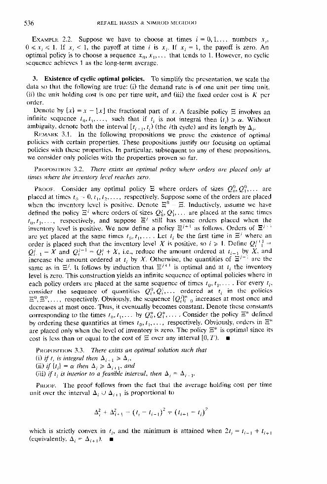
EXAMPLE 2.2. Suppose we have to choose at times i = 0,1,. . . numbers x,, 0 G x, G 1. If x , < 1, the payoff at time i is x,. If x i = 1, the payoff is zero. An optimal policy is to choose a sequence x,, x,, . . . that tends to 1. However, no cyclic sequence achieves 1 as the long-term average.

3. Existence of cyclic optimal policies. To simplify the presentation, we scale the data so that the following are true: (i) the demand rate is of one unit per time unit, (ii) the unit holding cost is one per time unit, and (iii) the fixed order cost is K per order.

Denote by ( X I = x - 1x1 the fractional part of x. A feasible policy E involves an infinite sequence to , t , , . . . , such that if ti is not integral then {t ,} >, a. Without ambiguity, denote both the interval [ t i - , , t i ) (the ith cycle) and its length by A;.

REMARK 3.1. In the following propositions we prove the existence of optimal policies with certain properties. These propositions justify our focusing on optimal policies with these properties. In particular, subsequent to any of these propositions, we consider only policies with the properties proven so far.

PROPOSITION 3.2. There exists an optimal policy where orders are placed only at times where the inventory level reaches zero.

PROOF. Consider any optimal policy 5 where orders of sizes Q:;, Q:, . . . are placed at times to = 0, t , , t,, . . . , respectively. Suppose some of the orders are placed when the inventory level is positive. Denote E0 = E. Inductively, assume we have defined the policy 8' where orders of sizes Qi, Q{, . . . are placed at the same times t,,, t , , . . . , respectively, and suppose 8' still has some orders placed when the inventory level is positive. We now define a policy EJfl as follows. Orders of Ei+' are yet placed at the same times t,,, t , , . . . . Let ti be the first time in El where an order is placed such that the inventory level X is positive, so i 2 1. Define Q!?: =

Q { _ , - X and Q{+l = Q/ + X, i.e., reduce the amount ordered at t i _ , by X, and increase the amount ordered at t , by X. Otherwise, the quantities of Ej+l are the same as in El. It follows by induction that El+' is optimal and at t i the inventory level is zero. This construction yields an infinite sequence of optimal policies where in each policy orders are placed at the same sequence of times t,,, t , , . . . . For every t i , consider the sequence of quantities Qy, Q,], . . . ordered at t , in the policies ';;o , , 30 , , . . . , respectively. Obviously, the sequence {Qj}lT=, increases at most once and

decreases at most once. Thus, it eventually becomes constant. Denote these constants corresponding to the times to , t , , . . . by Q:, Qy , . . . . Consider the policy Z* defined by ordering these quantities at times to , t , , . . . , respectively. Obviously, orders in E" are placed only when the level of inventory is zero. The policy E* is optimal since its cost is less than or equal to the cost of B over any interval [0, T ) .

PROPOSITION 3.3. There exists an optimal solution such that (i) if t , is integral then A;+ 2 Ai, (ii) if { t i} = a then A, > Ai+,, and (iii) if t i is interior to a feasible interval, then A, = A,+

PROOF. The proof follows from the fact that the average holding cost per time unit over the interval A, U A,,, is proportional to

which is strictly convex in t i , and the minimum is attained when 2ti = t i - l + t i+ , (equivalently, Ai = A,+ ,).


We now have to prove a certain property of shifts on the circle which helps when proving the existence of a cyclic optimal solution.

LEMMA 3.4. If a process is deJined on a circle by f ( 0 ) = 0 + a (mod 257) for some fied cr (and any starting point ), then

(i) the process is cyclic i f and only if u/n- is rational, (ii) i f u/n- is irrational, then for any startirzg point, every point on the circle is an

accumulation point.

PROOF. The proof of (i) is obvious. For the proof of (ii), suppose 0 is not an accumulation point. Thus there exists an interval I, of length E , centered at 0, which is not visited infinitely many times. This can happen only if the intervals Ij+ = I j + a

( j = 1,2, . . . ) are not visited infinitely many times. For some i and j, I, n I,,, + 0 and therefore I, n I, # 0. If I, = Zj then U / T must be rational. Otherwise, it follows that for some k the union of the intervals I,, . . . , Ik covers the entire circle, which is a contradiction.

DEFINITION 3.5. A value T is called feasible if the policy of A, = T for all i (i.e., t , = i T ) is feasible.

PROPOSITION 3.6. A oalue T is feasible if and only if T is a rational number that can be represented with a denominator less than or equal to l / a .

PROOF. Consider a mapping from the real line onto a circle so that a point t is mapped to the point at the angle 25-t (mod 277). If T is irrational then by Lemma 3.4 every point on the circle is an accumulation point. But if the policy is feasible then there exists an arc of positive length which is not visited and hence T is rational. Suppose T = J /N , where J and N are relatively prime. Obviously, for any j, {jT) is a multiple of l / N . Since there exist positive integers k and 1 such that kJ - 1N = 1, it follows that

Thus, for feasibility it is both necessary and sufficient that 1/N a. H

THEOREM 3.7. There exists an optimal solution where for infinitely many i's, { t , ) is either 0 or a .

PROOF. Consider any optimal solution (satisfying the properties discussed in Proposition 3.3). Suppose there is also only a finite number of i's such that { t i ) is either 0 or a. Consider the tail of the sequence where for all i, {t i) @ {O, a). By Proposition 3.3 we now have all the Ai's equal. We argue that in this case we can shift the tail of the solution so that all the ti's become integral. The proof is as follows. Since all the Ai's are equal to some T , it follows by Proposition 3.6 that T is rational with denominator N G l / a , and for infinitely many values of j, {jT) = l / N . It follows that we can shift the solution by the amount 1/N so that all the order times are feasible and an infinite number of them are integers. H

Below we consider the following four "finite" problems which we denote by P,,,, Pa,, P,,, and P,,,. These problems are useful in analyzing the optimal solutions for the whole problem.

DEFINITION 3.8. (i) The problem Po, is the following: find integers J and N such that the policy of N equally spaced orders over the interval [O, J ) (i.e., order every J/N time units) minimizes the average cost per time unit over such intervals, subject to the conditions that the initial inventory level is zero and orders are not placed during intervals of the form ( I , I + a) , where I is integer.

538 REFAEL HASSIN & NIMROD MEGIDDO

(ii) The problem Pa, is essentially the same as Po, except that the interval [O, J ) is replaced by [ a , J + a) .

(iii) The problem Po, is essentially the same as PO, except that the interval [O, J ) is replaced by [O, J + a) .

(iv) The problem P,, is essentially the same as Po, except that the interval [0, J ) is replaced by [ a , J ) .

Note that in the above problems we minimize over an infinite domain of values of T, so the existence of an optimal solution is not obvious. Furthermore, we show that the problems P,,, and Pa,, may not have optimal solutions. A value of T is said to be P,,,-feasible if there exist J and N for which the policy is feasible such that T = J / N .

PROPOSITION 3.9. Problem Po, has an optimal solution.

PROOF. Let T denote the length of the interval between consecutive orders, i.e., T = J/N. The average cost per time unit is therefore

The latter is a convex function of T and has a minimum at To = m. It follows from Proposition 3.6 that T is P,,,-feasible if and only if it is feasible (see Definition 3.5). In general, T,, may not be feasible. We are interested in the infimum of f(T) over all feasible values of T, i.e., T = J/N, where N G 1/a. Obviously, for each N, there is a minimum of f ( J /N) as a function of J and hence there exists a global minimum.

REMARK 3.10. The analysis of the problem P,, is essentially the same as Po,, namely, T is Pa,-feasible if and only if it is feasible, and hence it has an optimal solution. Moreover, the optimal solutions of PO,, and P,, have the same value.

REMARK 3.11. The problems PO, and P,, may not have optimal solutions. For example, consider PO, where a = 1/3 and the minimum of f (T) occurs at T, = 1/2. The latter is not P,,,-feasible since there do not exist integers J and N such that N/2 = J + 1/3. However, by choosing J arbitrarily large and N = 25 + 1, we obtain PO,-feasible policies with

arbitrarily close to To. We now analyze the sets of Po,-feasible and Pa,-feasible values. Denote by

0 = T(, < T , < r2 < . . . the feasible values of T (we include T = 0 for the ease of notation below). The properties of the Po,-feasible values, to be proven later (see Proposition 3.12), imply that these values can be enumerated in increasing order.

PROPOSITION 3.12. For eceiy i >, 1, if T, is not Po,-feasible, then there exist infinitely many PO,-feasible values between 7;- I and ri and the only accumulation point of this infinite set is 7,.

PROOF. Suppose T; is not Po,-feasible. We first show that T, is an accumulation point of PO,-feasible values less than 7,. Let E > 0 be any number such that E < T, - T,_ I . We argue that there exists a Po,-feasible value T such that ri - E < T < T,. Suppose ri - E is not Po,-feasible. Let N be the smallest integer such that 0 < {N(r, - 6)) < a , and let J = 1 N(ri - E ) J . Consider any value T such that ri - E

< T < ( J + a)/N; then O < {NT} < a, and hence T is not feasible. It follows that


Since there are no feasible values between T , - E and T ~ , it follows that for every j < N, jT is not an integer. Therefore, ( J + a ) / N is Po,-feasible.

Next, we show that there is no accumulation point of this set other than T ~ .

Consider any value T ' , < TI < 7;. Thus, T' is infeasible. We claim that there are only finitely many Po,-feasible values T such that T ~ - < T < TI. The proof is as follows. Let N ' be the smallest integer such 0 < { N ' T r ) < a , and let J' = [ N r T r ] . Imagine decreasing the value of T from T r . Denote T-= J r / N '. If T-< T < TI then 0 < { N r T ) < a. Thus, for such a T to be Po,-feasible, it is necessary that the corresponding value of N be less than N '. This implies that there are a finite number of Po,-feasible values between T - and T ' . If T - is feasible then T - = T , - I and we are done. Otherwise, there exist N - and J - less than N r and J', respectively, such that J-< N-T-< J-+ a . The above argument shows that there exist only finitely many Po,-feasible values of T between J - /N- and T-. The same argument can now be repeated. Every time we apply this argument the value of N ' decreases. Thus, the process terminates in a finite number of steps, and the total number of Po,-feasible values between 7, - , and T' is finite.

REMARK 3.13. It follows from the second part of the above proof that if 7, is Po,-feasible, then there exist only a finite number of Po,-feasible values between T ~ -

and T ~ .

PROPOSITION 3.14. For every i 2 1, if 7, - , is not Pa,-feasible, then there are infinitely many Pa,-feasible values between T ~ - and T~ and the only accumulation point of this inJinite set is T ~ - , . If T ~ - , is P,,-feasible, then there exist only a finite number of Pa,-feasible values between T~ - and 7,.

PROOF. This claim is analogous to those of Proposition 3.12 and Remark 3.13. We now show that the sequences of Po,-feasible values between two consecutive

feasible values 7,-, and T~ have special structures:

PROPOSITION 3.15. I f T~ = J/N (i 2 1; gcd(J, N ) = 1) is not Po,-feasible, then there exist numbers a = a(i) and b = b(i) such that the set of Po,-feasible values between T ~ - , and T , is the union of some finite set Si and the set of all the values of the .form

a + Jx + Nx , where x = 0,1 ,2 , . . . .

PROOF. We know that if T , is not Po,-feasible, then it is the only accumulation point of Po,-feasible values between T , ~ , and T , (Proposition 3.12). Let E > 0 be such that E < m i n ( ~ , - T , - , , a / N ) and let T ' be a Po,-feasible value such that T , - E < T r < 7,. Denote by S, the set of all Po,-feasible values T" such that T , -, < T" < T '. This set is finite. Let J' and N ' be such that T' = ( J ' + a ) / N t (thus, note that J' + a = NITr) . Since T , = J /N ,

and for any J , 0 < J < N, { J T ~ ) > 1 /N , so that

Since E < a / N , we have N T ~ > N T r > N T ; - NE > NT, - a , SO that

0 < ( ( N + N ' ) T J ) = { J ' + a + N T r ] < a


(i.e., T,, i = 1,2, is the length of the interval between consecutive orders over the first and the second intervals, respectively). The average cost over the interval [O, .I, + J,) is

Let A denote the infimum of the latter taken over all feasible choices of J,, N, (i = 1,2). Note that the claim applies to the case where the infimum is not attained. There exist sequences of values J,k, N,, tending to infinity with qk = J , ~ / N , ~ such that

(i) Kk tends to Tj*, (ii) f(T,,) tends to some limit f(T*), and (iii) the average cost

tends to A . By Propositions 3.12 and 3.14, the quantities T,* are feasible (in the sense of

Definition 3.5) and hence the average costs f(T,*) are greater than or equal to the minimum of the average cost taken over any policy with equally spaced orders. This minimum is precisely the minimum of P,,,,.

We can now prove the desired result:

THEOREM 3.21. There exists a cyclic optimal policy 5 where the defining cycle is an optimal solution of either Po, or Po,,,.

PROOF. By Theorem 3.7 there exists an optimal solution where for an infinite number of i's {ti} E {0, a ) . It suffices to consider the following three cases:

(i) For an infinite number of i's, ti is integral and for all i, {ti) # a . In this case the optimal value (of the long-term average cost) is a limit of weighted average of feasible values of problems of the form Po,,. By Proposition 3.9, the latter has an optimal solution. Thus, the cyclic solution consisting of repetitions of an optimal solution of Po, must be optimal.

(ii) For an infinite number of i's, {t,) = a and for all i (except for ti = 0), ti is not integral. In this case the solution starting with an order of a at time 0, and continuing with repetitions of an optimal solution of Pa,, must be optimal. Moreover, by shifting this solution we actually get the same cyclic solution as in (i).

(iii) For an infinite number of i's, t, is integral and for an infinite number of i's, {ti} = a . Consider an interval between two consecutive integral values t, , t,. Thus, there exist m values t,, t, < t, < t j ( m > O), such that {t,) = a and for any t, such that t, < t, < t,, {t,} Z 0. Suppose m > 2, and denote the points t, in [ti, t,] with {t,} = a by t,,, . . . , tk ,,,. The average cost per time unit over the interval [t,, t,) is a weighted average of two averages: c, over [r,,, tkm) and c, over the union of the intervals [t,, t,,) and [t,,,,, t,). Obviously, c, is greater than or equal to the optimum of the problem P,, (which is in turn equal to the optimum of Po,,), and c, is greater than or equal to the optimum of P,,,. It follows that the cyclic solution consisting of repetitions of the best of the optimal solutions (either of P,,, or of P,,,,,) must be optimal.

4. Computing an optimal policy. Having shown that a cyclic optimal solution exists, the natural question is whether an optimal cycle can be computed. The answer is not obvious since it requires a search over an infinite domain. For example, we

542 REFAEL HASSlN & NIMROD MEGIDDO

need to decide whether there exist feasible values

LZ + JX T = -- c + Jy

b + Nx and T - --- 2 - d + N y

( x and y integral) for Pa, and P,,, respectively, which together yield a solution of P ,,,, better than J / N , i.e.,

( a + J x ) f ( T , ) + ( c + J y I f ( T 2 ) ( a 1- Jx) + ( c + Jy)

This is the content of the following: PROBLEM 4.1. Given a , b, c, d , K , J , N > 0, recognize whether there exist nonneg-'

ative integers x and y such that

PROPOSITION 4.2. Problem 4.1 is decidable.

PROOF. A pair x , y > 0 solves the inequality of Problem 4.1 if and only if the following quantity is negative:

or, equivalently,

< ~ ( f - b ) + K(? - d ) .

The key observation here is that the function

is always monotone. It is increasing if J /N > a / b , constant if J / N = a / b , and decreasing if J / N < a /b . As x tends to infinity, g(x) tends to J /N. A similar observation holds for (c + Jy),/(d + Ny). All these imply that the left-hand side of ( * ) amounts to the sum of two monotone nonincreasing functions of x and y, respectively. Thus, the problem can be solved by letting x and y tend to infinity.

EXACT COMPUTATION O F OPTIMAL INVENTORY POI.ICIES 543

More precisely, the inequality of the problem has a solution if and only if

1 J (aN - bJ ) 1 J(cN - d l ) - . 2 ~2 + 2 ' N Z

If one wants to minimize $ ( x , y ) then the following procedure can be used. First, note the infimum is always less than or equal to the right-hand side, and we know how to decide whether it is strictly less than the latter. Assuming it is, for every value of x if suffices to check a finite number of values of y. As either x or y tends to infinity, the value of the left-hand side tends to that of the right-hand side, so after a finite number of steps the minimum is reached. However, we still have to develop the tools for recognizing the minimum when it is reached.

PROPOSITION 4.3. The infimum of $ ( x , y (see Problem 4.1) orler all nonnegatirse integers x , y is computable.

PROOF. It follows from Proposition 4.2 that if the minimum does not exist then the infimum is equal to f ( J / N ) = KN/J + ~ J / N . Thus we now assume the minimum exists and is less than f ( J / N ).

We first argue that for any E > 0 it can be decided whether there exist nonnegative integers x , y such that

The idea is essentially the same as that in the proof of Proposition 4.2. The problem is equivalent to deciding the existence of x , y such that

1 a + Jx aN - bJ 1 c + J y c N - d l ( * * ) z m . N + € ( a + Jx) + - 2 d + N y ------ . N + ~ ( c + Jy)

Here the left-hand side is a sum of functions g , ( x ) = g,(x; E ) and g,(y) = g , (y ; E ) .

Consider the function g, (x ) (the function g,(y) can be analyzed in the same way). If a / b = J /N the minimum of g , ( x ) is at x = 0. Otherwise, g , ( x ) is strictly convex with a unique minimum (over the reals) which can be derived analytically. The minimum of g , ( x ) over the nonnegative integers can then be found using a convexity argument. Thus, given any x and y we can decide whether they minimize +(x , y). So, assuming the minimum exists, by enumeration we reach it and recognize it.

REMARK 4.4. It is possible to develop a more efficient procedure for minimizing $ ( x , y). The question amounts to finding the maximum value E* of E for which the value of

is less than or equal to the right-hand side of ( * *). As the minimum of countably many linear functions, G ( E ) is monotone increasing and concave. When the minimum of +(x , y ) is strictly less than f ( J / N ) , we not only know that but we also find x , y such that $ ( x , y ) < f ( J / N ) . It follows that we can construct an interval containing E* over which G ( E ) has only finitely many pieces and hence using binary search we can locate E* exactly.

REMARK 4.5. A simpler problem can be handled essentially in the same way: given a , b , C, D , K, J, N > 0, recognize whether there exists a nonnegative integer x


such that

1 ( a + J X ) ~ K ( b + N x ) + 7 b + Nx + N I . /

< K - + 277' ( a + Jx) + D J

and if so, find the minimum of the left-hand side. Given feasible values T I = ( J l + a ) / N , and T2 = ( J 2 - a ) / N 2 of POU and Pa,,,

respectively, denote by

the value of the corresponding solution of PO,,,. Recall that TO = v ' 2 ~ minimizes K / T + +T over the reals arid 0 = T,, < T , < . . . are the feasible values, i.e., rationals with denominators less than or equal to l / u .

PROPOSITION 4.6. Suppose 7,-I < TO < 7, and let T I = ( J , + u ) / N , be any P ,,,, - feasible value in the intercal (TO, T,). Let T2 = ( J , - u ) / N , denote the maximal Pa,,-feasible value in the intercar' [ T , , T , + , ). Under these conditions,

4 ( J , , hi,; J,', N; ) > 4 ( J , , N , ; J2,N2)

for any Pa,,-feasible calue T,' = (J,' - u)/N,' such that either (i) T; > J , - u or (ii) J,' > J , and T i 2 T , + ,.

PROOF. The assumptions on T I and T2 imply f ( T , ) < f (T2 ) . Thus 4 will increase if J, and N, are replaced by J,' and N; such that J,' > J2 and f ( J ; /N; ) > f(J,/N,). In case (i) the claim follows from the inequalities.

J i - u > T ; > J 2 - u and T , ' > J 2 - u 2 T 2 .

The proof of case (ii) is similar.

COROLLARY 4.7. Assume [he conditions of Proposition 4.6, and f ( ~ , ) < f ( r , - ,). Given any POa-feasible value T I = ( J , + u ) / N , such that f ( T l ) < F,,,,, in order to decide whether 4 ( J , , N,; J,, N,) < F,, for some Pa,,-feasible pair ( J , , N,), it sufices to consider candidates T2 = ( J2 - a) /N2 only from a union of a finite number of interr.als of the form [T,- ,, T,), and except for the case k = i + 1, in each interval only a finite number of values need to be considered.

PROOF. The sequence of Pa,-feasible values which lie between two consecutive values T , ~ , and T , (see Proposition 3.16) accumulates into 7,-,. There are only a finite number of k's such tlhat k < i . If k < i then the value 4 ( J 1 , N l ; J,, N 2 ) increases as the value T , = ( J , - a ) / N 2 varies along the sequence. So, it suffices to check the first member of the sequence (as well as the finite number of values not in the sequence which lie in the same interval). Similarly, if k = i , it suffices to check among the members of the structured sequence only the values of T, which are greater than or equal to T , (there are only finitely many of these) and the largest one which is less than TO. If k > i + 1, then the claim follows from Proposition 4.6.

REMARK 4.8. The number of values considered in Corollary 4.7 can be further reduced by noting that T = J / N is PO,-feasible if and only if T + 1 = ( N + J ) / N is. Now, if T,' > To + 1 then 4(.T,, N,; J,' - N,', N,') < +(J,, N,; J ; , N,'). Thus only values less than To + 1 need to be checked. A similar argument shows that if suffices to consider only values greater tlhan T, - 1.

5. Summary of the algorithm. We now sketch an algorithm for an optimal policy. Most of the effort in the algorithm goes into the determination of whether

EXACT COMPUTATION OF OPTIMAL INVENTORY POLICIES 5 45

F,,, < Fo,. Indeed, if this inequality holds and a feasible solution with $(J,, N,; J,, N,) < Fo, is known then, as we argue below, there remain only a finite number of solutions of POa, that have to be checked before the optimal solution is found. The main steps of the algorithm are as follows.

(i) The first step is to calculate the minimum TO = m. If TO is rational with denominator N G l / a then the policy of ordering every T, time units is optimal. Otherwise, find two nonnegative rationals r i - ] , r i (see the definition preceding Proposition 3.12) with denominators not greater than l / a , such that rip, < T, < T,. The optimal solution of P,, (see Definition 3.8) is determined by either ri-, or T,, i.e., Fu() = min{f(ri-,), f ( ~ , ) ) .

(ii) In this step, we construct ((in the sense of Remark 3.17) the sets of feasible solutions of P,, and P,,, which lie strictly between .rip, and 7,. If there are no feasible T's neither for PO, nor. for Pa, such that f (T) < FO,, then the optimal solution for the whole problem is the optimal solution of P,, found in (i), so we stop. Otherwise, we continue with step (iii).

(iii) We now determine whether Fo,, < Fo,. We do this by analyzing the neighbor- hood of T,-, or T,, or both (depending on how Po,, is attained as the minimum of f ( ~ ; - ~ ) and f ( ~ ~ ) ) . Consider the case where f ( ~ , ) = FO,, < f ( ~ , - ~ ) ; the other cases are handled analogously. Suppose there exists a feasible value TI = ( J , + a)/N, of POa such that f(T,) < F,,, so T, lies strictly between T,-] and 7,. Given TI we search for feasible values T2 = (J, - a)/N, of Pa() SO as to minimize the value +(.TI, N,; J,, N,) of the corresponding solution of lD,,,. This is done as follows. We are interested only in T, = (J, - a)/N, such that c$(J,, N,; J,, N,) < F,,. Proposition 4.6 (case (i)) explains how to bound the number of intervals [ r k p l , r k ) that have to be checked, so we can restrict attention to a finite set of such intervals. Suppose first that k # i + 1; the case k = i = 1 is discussed in (iv). By Corollary 4.7, in each interval there is only a finite number of points that have to be considered. For each possible value of T,, we consider all the values of T, between 7,-, and ri which are Po,-feasible. Here we rely on Remark 4.5 for finding th~e optimal TI or concluding that the infimum is not less than F,,,,.

(iv) Now we consider the case k = i + 1. Here we have to consider an infinite number of values of both TI and T,. The two sequences tend to 7,- I from different sides. We rely on Proposition 4.3 and either find an optimal pair T,, T, or conclude that no such pair gives a value less than F,,.

6. Finding a good approxima~te solution. If one is satisfied with approximately optimal policies then the following proposition is useful. We know that the optimal value is the minimum of F,, and F,,,,. If F,,, (which is easy to compute) is taken as an approximately optimal solution, the error can be estimated as follows.

PROPOSITION 6.1. If J , , N, ( i = 1,2) define an optimal solution for Po,,, such that

then the aaerage cost per time unit in this solution, F,,,, and the optimal average cost per time unit, F[,[,, in Po,) satisfy


PROOF. Denote by T the smallest value greater than T, = ( J , + cr)/N, which is feasible (for P,,), i.e.., it is rational with denominator not greater than l / a . Note that

since N , times the right-hand side is an integer. Actually, if T = j/n (gcd( j, n) = I), then by the classical Dirichlet's theorem,

Acknowledgements. We are grateful to Dafna Sheinwald for pointing out a delicate flaw in one of the proofs in an earlier version.

References [ I ] Andres, F. M. and Emmons, H. (1976). On the Optimal Packaging Frequency of Products Jointly

Replenished. Management S<ci. 22 1165-1166. [2] Buzacott, J. A. and Ozkarahan, I. A. (1983). One and Two-Stage Scheduling of Two Products with

Distributed Inserted Idle T h e : The Benefits of a Controllable Production Rate. Nacal Res. Logist. Quart. 30 675-696.

131 Dobson, G. (1987). The Economic Lot-Scheduling Problem: Achieving Feasibility using Time-Varying Lot Sizes. Oper. Res. 35 764-771.

[4] Elmaghraby, S. L. (1978). The Economic Lot Scheduling Problem (ELSP): Review and Extensions. Management Sci. 24 587-598.

[5] Graves, S. C. (1981). A Review of Production Scheduling. Oper. Res. 29 646-675. [6] Maxwell, W. L. and Singh, H. (1983). The Effect of Restricting Cycle Times in the Economic Lot

Scheduling Problem. IIE Trans. 15 235-241.

[7] Muckstadt, J. A. and Singer, H. M. (1978). Comments on Single Qc le Continuous Review Policies for Arborescent Production/Inventory Systems. Management Sci. 24 1766-1768.

[81 Roundy, R. (1986). A 98-Percent-Effective Lot-Sizing Rule for a Multi-Product, Multi-Stage Produc- tion Inventory System. Math. Oper. Res. 11 699-727.

191 Schweitzer, P. J. and Silver. E. A. (1983). Mathematical Pitfalls in the One Machine Multi-Product Economic Lot Scheduling Problem. Oper. Res. 31 401-405.

HASSIN: SCHOOL O F MA.THEMATICS, TEL AVIV UNIVERSITY, TEL AVIV 69978, ISRAEL

MEGIDDO: IBM RESEARCH DIVISION, ALMADEN RESEARCH CENTER, SAN JOSE, CALI- FORNIA 95120-6099

SCHOOL O F MATHEMATICAL SCIENCES, TEL AVIV UNIVERSITY, TEL AVIV 69978, ISRAEL

Documents

exact computation of optimal inventory policies over an unbounded