Embed Size (px)
Citation preview

Exact Distribution of the Mean Reversion Estimator in
the Ornstein-Uhlenbeck Process∗
Yong Bao†
Department of Economics
Purdue University
Aman Ullah‡
Department of Economics
University of California, Riverside
Yun Wang§
School of International Trade and Economics
University of International Business and Economics
August 31, 2014
Abstract: Econometricians have recently been interested in estimating and testing the mean reversion param-eter (κ) in linear diffusion models. It has been documented that the maximum likelihood estimator (MLE) of κtends to over estimate the true value. Its asymptotic distribution, on the other hand, depends on how the dataare sampled (under expanding, infill, or mixed domain) as well as how we spell out the initial condition. Thisposes a tremendous challenge to practitioners in terms of estimation and inference. In this paper, we providenew and significant results regarding the exact distribution of the MLE of κ in the Ornstein-Uhlenbeck processunder different scenarios: known or unknown drift term, fixed or random start-up value, and zero or positive κ.In particular, we employ numerical integration via analytical evaluation of a joint characteristic function. Ournumerical calculations demonstrate the remarkably reliable performance of our exact approach. It is found thatthe true distribution of the MLE can be severely skewed in finite samples and that the asymptotic distributionsin general may provide misleading results. Our exact approach indicates clearly the non-mean-reverting behav-ior of the real federal fund rate.
JEL Classification: C22, C46, C58
Key Words: Distribution, Mean Reversion Estimator, Ornstein-Uhlenbeck Process
∗We are thankful to Yacine Aıt-Sahalia, Peter Phillips, and Jun Yu, for helpful comments. We also benefited from discussionswith Victoria Zinde-Walsh on the subject matter.†Corresponding Author: Department of Economics, Purdue University, 403 W. State Street, West Lafayette, IN 47907, USA.
E-mail: [email protected].‡Department of Economics, University of California, Riverside, CA 92521, USA. E-mail: [email protected].§School of International Trade and Economics, University of International Business and Economics, Beijing, China. E-mail:
1 Introduction
Since the seminal works of Merton (1971) and Black and Scholes (1973), continuous-time models have been used
extensively in financial economics, see the excellent survey by Sundaresan (2000). Econometricians have also
paid close attention to this line of literature. Maximum likelihood, generalized method of moments, simulated
method of moments, and nonparametric approaches have been developed for model estimation, see, for instance,
Singleton (2001), Bandi and Phillips (2003), Hong and Li (2005), and Phillips and Yu (2009a).
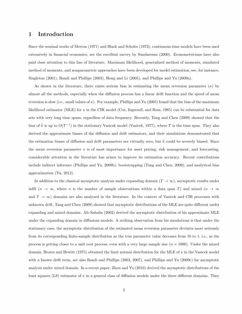
As shown in the literature, there exists serious bias in estimating the mean reversion parameter (κ) by
almost all the methods, especially when the diffusion process has a linear drift function and the speed of mean
reversion is slow (i.e., small values of κ). For example, Phillips and Yu (2005) found that the bias of the maximum
likelihood estimator (MLE) for κ in the CIR model (Cox, Ingersoll, and Ross, 1985) can be substantial for data
sets with very long time spans, regardless of data frequency. Recently, Tang and Chen (2009) showed that the
bias of κ is up to O(T−1) in the stationary Vasicek model (Vasicek, 1977), where T is the time span. They also
derived the approximate biases of the diffusion and drift estimators, and their simulations demonstrated that
the estimation biases of diffusion and drift parameters are virtually zero, but κ could be severely biased. Since
the mean reversion parameter κ is of most importance for asset pricing, risk management, and forecasting,
considerable attention in the literature has arisen to improve its estimation accuracy. Recent contributions
include indirect inference (Phillips and Yu, 2009b), bootstrapping (Tang and Chen, 2009), and analytical bias
approximation (Yu, 2012).
In addition to the classical asymptotic analysis under expanding domain (T →∞), asymptotic results under
infill (n → ∞, where n is the number of sample observations within a data span T ) and mixed (n → ∞
and T → ∞) domains are also analyzed in the literature. In the context of Vasicek and CIR processes with
unknown drift, Tang and Chen (2009) showed that asymptotic distributions of the MLE are quite different under
expanding and mixed domains. Aıt-Sahalia (2002) derived the asymptotic distribution of his approximate MLE
under the expanding domain in diffusions models. A striking observation from his simulations is that under the
stationary case, the asymptotic distribution of the estimated mean reversion parameter deviates more seriously
from its corresponding finite-sample distribution as the true parameter value deceases from 10 to 1, i.e., as the
process is getting closer to a unit root process, even with a very large sample size (n = 1000). Under the mixed
domain, Brown and Hewitt (1975) obtained the limit normal distribution for the MLE of κ in the Vasicek model
with a known drift term, see also Bandi and Phillips (2003, 2007), and Phillips and Yu (2009c) for asymptotic
analysis under mixed domain. In a recent paper, Zhou and Yu (2010) derived the asymptotic distributions of the
least squares (LS) estimator of κ in a general class of diffusion models under the three different domains. They
2

provided Monte Carlo evidence that the infill asymptotic distribution is much more accurate in approximating
the true finite-sample distribution than the asymptotic distributions under the other two domains.
The problems of estimation bias and inaccurate and different distribution approximations floating in the
literature are largely due to the absence of exact analytical distribution results. Moreover, in reality, given the
discretized data (with a given finite data span T and finite sample size n ), we do not really know under which
asymptotic domain our inference about κ shall be, but the asymptotic distribution results can behave quite
differently under expanding, infill, and mixed domains. To address these problems, in this paper we investigate
the exact distribution of the estimated mean reversion parameter in the Ornstein-Uhlenbeck process. To the
best of our knowledge, our paper is the first to examine the exact finite-sample distribution of the estimated κ in
continuous-time models. Since the MLE of κ is a simple transformation of the LS estimator of the autoregressive
coefficient φ in a first-order autoregressive (AR(1)) model with discrete data, our study is intrinsically related
to the vast literature studying the finite-sample distribution of the AR(1) coefficient estimator φ. The Imhof
(1961) technique, in conjunction with Davies (1973, 1980), was typically used to develop the exact distribution
of φ, see Ullah (2004) for a comprehensive review. Nevertheless, the Imhof (1961) technique is applicable only
when the process is strictly stationary with an initial random observation included in formulating φ, or when the
first observation is discarded. Computational burden of the Imhof (1961) technique also increases tremendously
as the sample size of the AR process increases, since it involves computation of eigenvalues of a matrix whose
dimension is the same as the sample size. In this paper, we take a different approach by first analytically
evaluating the joint characteristic function of the random numerator and denominator in defining φ, and then
inverting it via Gurland (1948) and Gil-Pelaez (1951) to calculate the exact finite-sample distribution. This
approach is in line with Tsui and Ali (1992, 1994) and Ali (2002). However, note that in Tsui and Ali (1992,
1994) and Ali (2002), no intercept term was included in the AR(1) model. This is equivalent to a known
drift term in the linear diffusion process. In this paper, we consider explicitly the case when the drift term is
unknown. Moreover, Tsui and Ali (1992, 1994) did not include the initial observation in formulating the LS
estimator φ, whereas Ali (2002) focused on the approximate distribution with the initial observation included.
The initial observation does matter in studying the exact distributions in finite samples; in fact, it also matters
even for the asymptotic distributions under several scenarios.
The remainder of our paper is as follows. In Section 2, we derive the exact distribution of the MLE of the
mean reversion parameter κ. We also presents simulation results and compare our exact distribution results
with the asymptotic results under the three different domains. In Section 3 we construct the exact confidence
intervals for the mean reversion parameter κ when the linear diffusion model is used to study the real federal
3

fund rate, and we find strong evidence of the non-mean-reverting behavior. Section 4 concludes. Technical
details are collected in the appendix.
2 Exact Distribution
We consider the Ornstein-Uhlenbeck (OU) process with the initial value x(0),
dx(t) = κ(µ− x(t))dt+ σdB(t), (2.1)
where κ ∈ R, µ ∈ R, σ > 0, and B(t) is a standard Brownian motion. We are interested in estimating the
parameter κ. When κ 6= 0, the solution to the above process is
x(t) = µ+ (x(0)− µ) exp (−κt) + σ
∫ t
0
exp (κ(s− t)) dB(s), t ≥ 0. (2.2)
Usually κ > 0 is assumed, and then as t→∞, the deterministic part of x tends to the mean level µ, so we have
a mean-reverting process. When κ = 0, the process is no longer mean reverting:
x(t) = x(0) + σB(t), (2.3)
where the parameter µ vanishes.
In practice, the observed data are discretely recorded at (0, h, 2h, · · · , nh) in the time interval [0, T ], where
h is the sampling interval and T is the data span. The exact discrete model corresponding to (2.1) is an AR(1)
model:
xih = α+ φx(i−1)h + εih, i = 0, 1, · · · , n, (2.4)
where φ = exp(−κh), α = µ[1−exp(−κh)], and εih ∼ i.i.d.N(0, σ2ε). The definition of the error term εih depends
on whether κ is positive or zero: εih = σεi√
(1− exp(−2κh))/(2κ) when κ > 0, εih = σ√hεi when κ = 0, where
εi ∼ i.i.d.N(0, 1). Correspondingly, σ2ε = σ2(1 − exp(−2κh))/(2κ) when κ > 0 and σ2
ε = σ2h when κ = 0.
Note that the autoregressive coefficient φ is always positive by definition. When κ = 0, φ = 1, α = 0, so (2.4)
becomes a random walk (with no drift). In the sequel, we suppress h in xih and εih for notational convenience.
It is well known that the LS/ML estimator of κ based on the discrete data is
κ = − ln(φ)
h, (2.5)
4
where φ is the LS estimator of φ in (2.4). When µ is known (without loss of generality, µ = 0), φ =∑ni=1 xi−1xi/
∑ni=1 x
2i−1; for the case of unknown µ, φ =
∑ni=1(xi−1 − x)xi/
∑ni=1(xi−1 − x)2, where x =
n−1∑ni=1 xi−1.
1
We are interested in studying the properties of κ estimated from the discrete sample via φ. As can be
expected, the exact properties of κ depend on how we spell out the initial observation x(0) = x0. It can be fixed
(at zero or a non-zero constant) or random. In this paper, when x0 is random, we assume that the time series
(x0, x1, · · · , xn) is stationary.
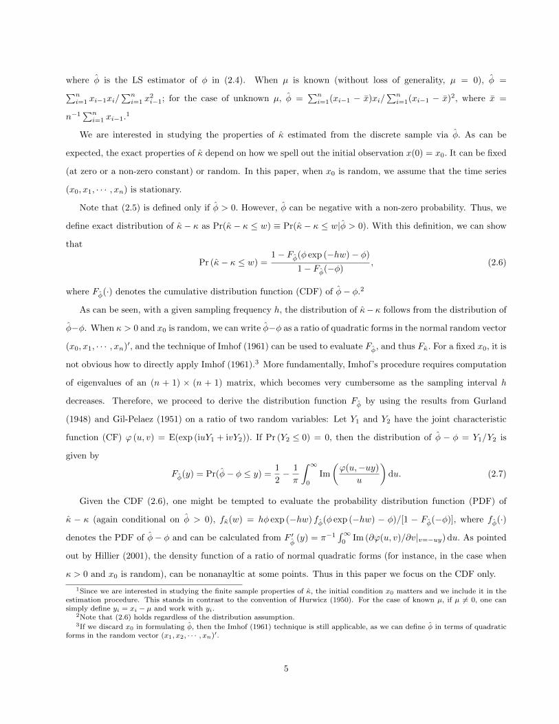
Note that (2.5) is defined only if φ > 0. However, φ can be negative with a non-zero probability. Thus, we
define exact distribution of κ− κ as Pr(κ− κ ≤ w) ≡ Pr(κ− κ ≤ w|φ > 0). With this definition, we can show
that
Pr (κ− κ ≤ w) =1− Fφ(φ exp (−hw)− φ)
1− Fφ(−φ), (2.6)
where Fφ(·) denotes the cumulative distribution function (CDF) of φ− φ.2
As can be seen, with a given sampling frequency h, the distribution of κ−κ follows from the distribution of
φ−φ. When κ > 0 and x0 is random, we can write φ−φ as a ratio of quadratic forms in the normal random vector
(x0, x1, · · · , xn)′, and the technique of Imhof (1961) can be used to evaluate Fφ, and thus Fκ. For a fixed x0, it is
not obvious how to directly apply Imhof (1961).3 More fundamentally, Imhof’s procedure requires computation
of eigenvalues of an (n + 1) × (n + 1) matrix, which becomes very cumbersome as the sampling interval h
decreases. Therefore, we proceed to derive the distribution function Fφ by using the results from Gurland
(1948) and Gil-Pelaez (1951) on a ratio of two random variables: Let Y1 and Y2 have the joint characteristic
function (CF) ϕ (u, v) = E(exp (iuY1 + ivY2)). If Pr (Y2 ≤ 0) = 0, then the distribution of φ − φ = Y1/Y2 is
given by
Fφ(y) = Pr(φ− φ ≤ y) =1
2− 1
π
∫ ∞0
Im
(ϕ(u,−uy)
u
)du. (2.7)
Given the CDF (2.6), one might be tempted to evaluate the probability distribution function (PDF) of
κ − κ (again conditional on φ > 0), fκ(w) = hφ exp (−hw) fφ(φ exp (−hw) − φ)/[1 − Fφ(−φ)], where fφ(·)
denotes the PDF of φ− φ and can be calculated from F ′φ
(y) = π−1∫∞0
Im (∂ϕ(u, v)/∂v|v=−uy) du. As pointed
out by Hillier (2001), the density function of a ratio of normal quadratic forms (for instance, in the case when
κ > 0 and x0 is random), can be nonanayltic at some points. Thus in this paper we focus on the CDF only.
1Since we are interested in studying the finite sample properties of κ, the initial condition x0 matters and we include it in theestimation procedure. This stands in contrast to the convention of Hurwicz (1950). For the case of known µ, if µ 6= 0, one cansimply define yi = xi − µ and work with yi.
2Note that (2.6) holds regardless of the distribution assumption.3If we discard x0 in formulating φ, then the Imhof (1961) technique is still applicable, as we can define φ in terms of quadratic
forms in the random vector (x1, x2, · · · , xn)′.
5

2.1 Joint Characteristic Function
For us to be able to use (2.7) to derive (2.6) for κ − κ, an essential task is to evaluate the joint characteristic
function of the numerator and denominator in defining φ − φ. To facilitate presentation, we first introduce
some notation. Let 0n be an n × 1 vector of zeros, In be the identity matrix of size n, ιn be an n × 1 vector
of ones, Mn = In − n−1ιnι′n, ei,n be a unit/elementary vector in the n-dimensional Euclidean space with its
i-th element being 1. Given an (n− 1)× (n− 1) matrix Cn−1, we define ACn as an n× n matrix with its lower
left block being Cn−1 and all other elements being zero, and BCn as an n× n matrix with its upper left block
being Cn−1 and all other elements being zero. When Cn−1 = In−1, we simply put An = AIn and Bn = BI
n.
For an n× n matrix Cn, we use cn,ij to denote its ij-th element, and c(ij)n to denote the ij-th element of C−1n ,
whenever it exists. Throughout, V n is an n× n matrix with its ij-th element φ|i−j|.
When κ > 0, define zi = (xi−µ)/σε, i = 0, · · · , n, and z = n−1∑ni=1 zi−1.Obviously, φ =
∑ni=1 zi−1zi/
∑ni=1 z
2i−1
for the case of known µ, and φ =∑ni=1(zi−1 − z)zi/
∑ni=1(zi−1 − z)2 for the case of unknown µ.
In the case of κ = 0, the parameter µ vanishes, and we define zi = xi/σε and ¯z = n−1∑ni=1 zi−1. In practice,
we may still proceed to estimate φ from the discrete AR(1) model without or with an intercept even when the
parameter µ is not defined. Correspondingly, φ =∑ni=1 zi−1zi/
∑ni=1 z
2i−1 or φ =
∑ni=1(zi−1− ¯z)zi/
∑ni=1(zi−1−
¯z)2.
Denote zn = (z1, · · · , zn)′ and ζn+1 = (z0, zn)′. Note that (z2, · · · , zn)′ = (0n−1, In−1) zn, (z1, · · · , zn−1)′ =
(In−1,0n−1) zn, and (z0 − z, · · · , zn−1 − z)′ = MnAnzn+z0Mne1,n. (Results pertaining to z can be obviously
defined.) Thus we can express the following sums in matrix notation:∑ni=1 zi−1zi = z0z
′ne1,n + z′nAnzn = ζ′n+1An+1ζn+1,∑n
i=1 z2i−1 = z20 + z′nBnzn = ζ′n+1Bn+1ζn+1,∑n
i=1(zi−1 − z)zi = z′nMnAnzn + z0z′nMne1,n = ζ′n+1A
Mn+1ζn+1,∑n
i=1(zi−1 − z)2 = z′nA′nMnAnzn + z20e
′1,nMne1,n + 2z0z
′nA′nMne1,n = ζ′n+1B
Mn+1ζn+1.
Consequently, when κ > 0, we can write the numerator and denominator (Y1 and Y2) in formulating
φ − φ in terms of quadratic forms in either zn (when x0 is fixed) or ζn+1 (when x0 is random). Define
the following matrices/vectors (note that these matrices and vectors depend on u, v, and model parameters; we
have suppressed their arguments):
Rn = In +(φ2 + 2iuφ− 2iv
)Bn − (φ+ iu) (An +A′n),
δn = iu(In − 2φA′n)Mne1,n + 2ivA′nMne1,n + φe1,n,
Sn = In + φ2Bn − φ(An +A′n)− iu(MnAn +A′nMn) + 2i(uφ− v)A′nMnAn,
T n+1 = (1− φ2)V −1n+1 − iu(AMn+1 +AM ′
n+1) + 2i(uφ− v)BMn+1.
6
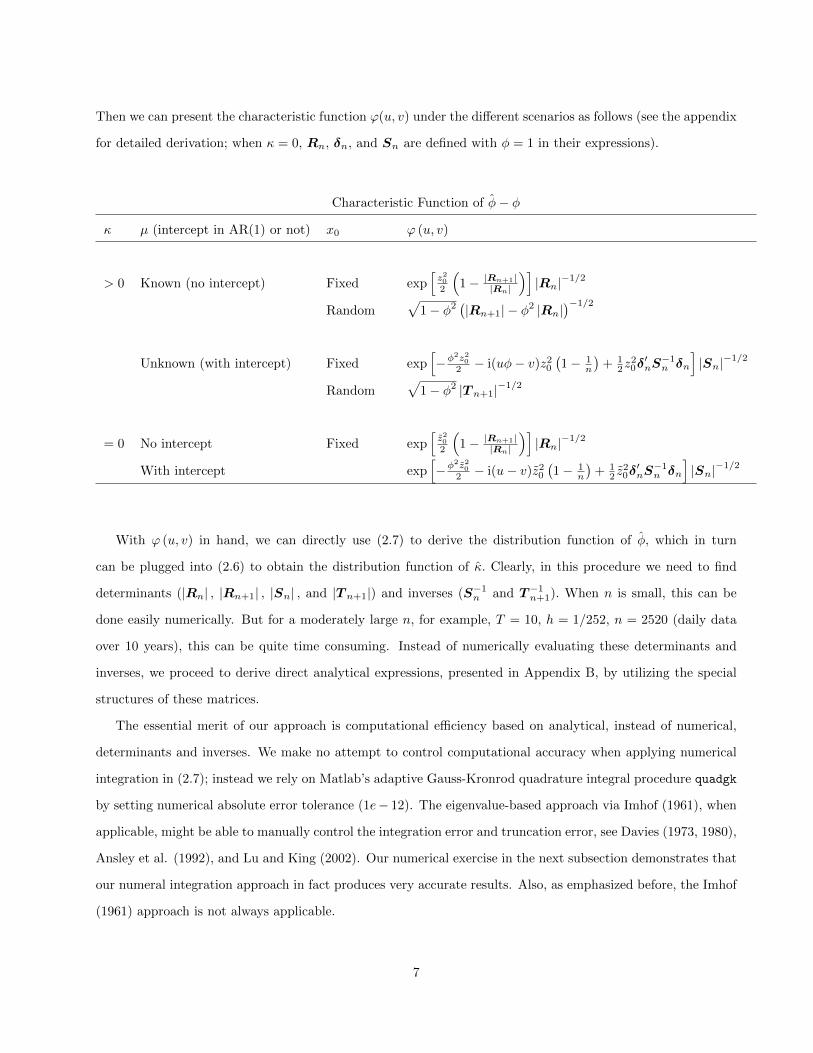
Then we can present the characteristic function ϕ(u, v) under the different scenarios as follows (see the appendix
for detailed derivation; when κ = 0, Rn, δn, and Sn are defined with φ = 1 in their expressions).
Characteristic Function of φ− φ
κ µ (intercept in AR(1) or not) x0 ϕ (u, v)
> 0 Known (no intercept) Fixed exp[z202
(1− |Rn+1|
|Rn|
)]|Rn|−1/2
Random√
1− φ2(|Rn+1| − φ2 |Rn|
)−1/2Unknown (with intercept) Fixed exp
[−φ
2z202 − i(uφ− v)z20
(1− 1
n
)+ 1
2z20δ′nS−1n δn
]|Sn|−1/2
Random√
1− φ2 |T n+1|−1/2
= 0 No intercept Fixed exp[z202
(1− |Rn+1|
|Rn|
)]|Rn|−1/2
With intercept exp[−φ
2z202 − i(u− v)z20
(1− 1
n
)+ 1
2 z20δ′nS−1n δn
]|Sn|−1/2
With ϕ (u, v) in hand, we can directly use (2.7) to derive the distribution function of φ, which in turn
can be plugged into (2.6) to obtain the distribution function of κ. Clearly, in this procedure we need to find
determinants (|Rn| , |Rn+1| , |Sn| , and |T n+1|) and inverses (S−1n and T−1n+1). When n is small, this can be
done easily numerically. But for a moderately large n, for example, T = 10, h = 1/252, n = 2520 (daily data
over 10 years), this can be quite time consuming. Instead of numerically evaluating these determinants and
inverses, we proceed to derive direct analytical expressions, presented in Appendix B, by utilizing the special
structures of these matrices.
The essential merit of our approach is computational efficiency based on analytical, instead of numerical,
determinants and inverses. We make no attempt to control computational accuracy when applying numerical
integration in (2.7); instead we rely on Matlab’s adaptive Gauss-Kronrod quadrature integral procedure quadgk
by setting numerical absolute error tolerance (1e− 12). The eigenvalue-based approach via Imhof (1961), when
applicable, might be able to manually control the integration error and truncation error, see Davies (1973, 1980),
Ansley et al. (1992), and Lu and King (2002). Our numerical exercise in the next subsection demonstrates that
our numeral integration approach in fact produces very accurate results. Also, as emphasized before, the Imhof
(1961) approach is not always applicable.
7

2.2 Numerical Results
In this section, we conduct Monte Carlo simulations to illustrate the finite sample performance of our exact
distribution in comparison with the “true” distribution and the asymptotic distribution. The data generating
process follows the OU model in (2.4), and the error term is generated from a normal distribution. The
asymptotic distribution results are available from Zhou and Yu (2010).4 Note that under the infill asymptotics,
the results are conditional on the initial x0.
We set T = 1, 2, 5, 10, h = 1/12, 1/52, 1/252, κ = 0.01, 0.1, 1, µ = 0, 0.1, σ = 0.1, x0 = µ or x0 ∼
N(µ, σ2/(2κ)). Compared with Zhou and Yu (2010), we have a more comprehensive experiment design, so as
to have a better understanding of the finite-sample distributions. For the fixed start-up case (x0 = 0), we also
consider κ = 0. As pointed out in Zhou and Yu (2010), the values of 0.01 and 0.1 for κ are empirically realistic
for interest rate data while the value of 1 is empirically realistic for volatility.
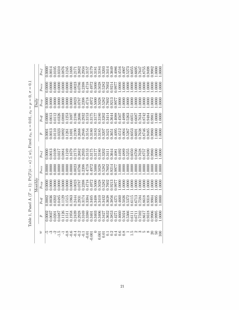
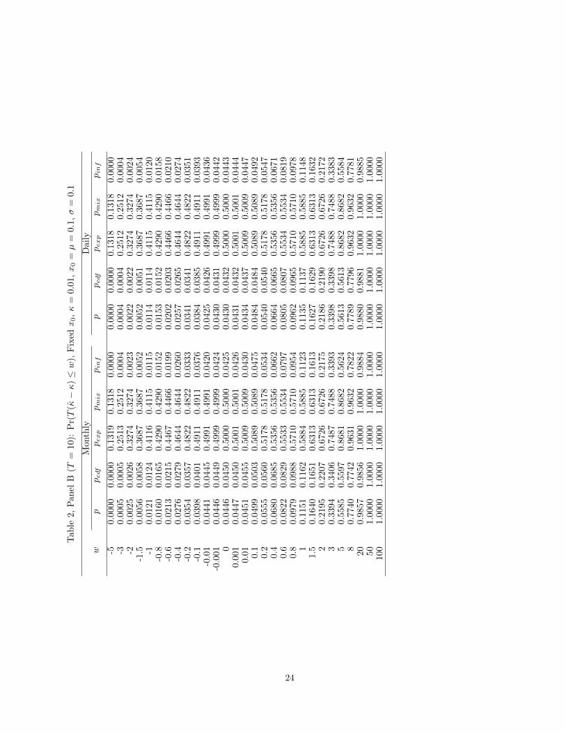
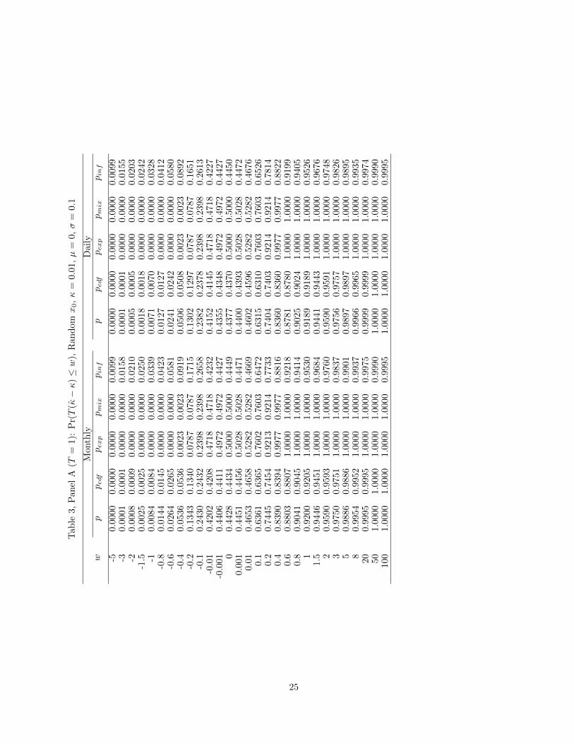
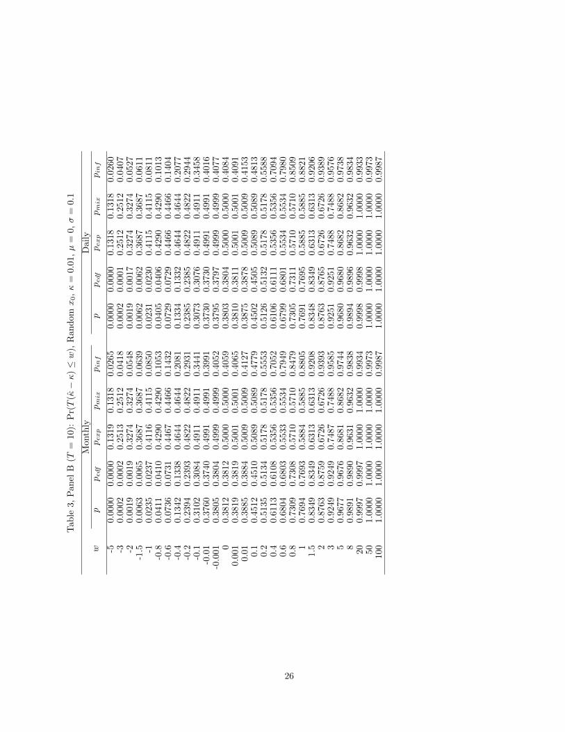
Tables 1–4 report the cumulative distributions of T (κ− κ), where the “true” distribution results come from
1,000,000 replications, and we make comparison of the exact (p), true (pedf ), and asymptotic results under the
three asymptotics (pexp, pmix, pinf ).5 In calculating the exact distribution with the analytical characteristic
function, we still need to implement numerical integration in (2.7). Appendix C discusses how to overcome
the problem of discontinuity of the square root function in the complex domain. The complete experiment
results are available from the corresponding author upon request. To save space, we report only the results for
h = 1/12, 1/252 in Tables 1–4 (each with two panels corresponding to T = 1, 10, respectively). Tables 1 and
2 report the cumulative distributions of T (κ− κ) under a fixed start-up when κ = 0.01, with x0 = µ = 0, 0.1,
respectively, and Tables 3 and 4 report the results when x0 is random.
Several striking features are present in these tables. First, the exact distribution results match to at least
the third decimal place with those obtained by 1 million simulations, in all the cases considered. This indicates
high accuracy of the exact results calculated by our numerical integration algorithm. In consistent with the
asymptotic results in Zhou and Yu (2010), there is no much difference between the results under the expanding
and mixed domains, and the infill asymptotics provide relatively better performance. Yet, the asymptotic
distribution under the infill domain may still provide poor approximation to the true distribution when the
data span is short, especially so in the left tails. While increasing data frequency does not affect much the
4Zhou and Yu (2010) did not give the expanding and infill asymptotic distribution results when κ = 0 and µ 6= 0. Thiscorresponds to the scenario, in a discrete framework, when no intercept is present in the true model, but a constant term isincluded in the regression. The expanding and infill asymptotic distribution results easily follow via the generalized delta method.
5In simulating the asymptotic (non-normal) results, 10,000 replications are used and a sample size of 5,000 is used to approximatethe integrals involving the Brownian motion by the discrete Riemann sums, with the exception that the infill asymptotic resultswhen x0 is random are calculated as averaging over 2,000 replications, where in each replication, x0 ∼ N(µ, σ2/(2κ)) and thediscrete AR(1) process is of sample size of 2,000.
8

asymptotic distributions, it does affect the true distribution, and the remarkable performance of the exact
distribution is robust to data frequency, as well as to data span and other aspects of model specification.
Second, the true distribution of κ is highly skewed to the right. Normality is a terrible approximation of the
finite-sample distribution of κ. Moreover, we can infer from these tables the exact/true median of T (κ− κ) in
all cases are substantially positive. (A direct calculation of the median is also possible, see the last paragraph
in this section to follow.) This suggests that κ can significantly over estimate κ in finite samples. This degree
of overestimation does not decrease with a higher data frequency (given a fixed data span). This is in line with
the observations made by Phillips and Yu (2005) and Tang and Chen (2009). On the other hand, increasing
data span might help alleviate this problem, though somewhat marginally.
Third, how the initial observation is spelled out affects significantly the exact distribution of κ. For example,
for the fixed start-up case, the exact distribution is less skewed to the right when x0 = 0 compared with when
x0 6= 0. Comparing the random start-up case versus the fixed start-up case with a known drift term (Table
3 versus Table 1), we see quite a difference in the exact distributions across the two cases and the former one
is less skewed; on the other hand, with a unknown drift term (Table 4 versus Table 2), there is virtually no
significant difference in the exact distributions across the two cases.6 This feature is related to the role of initial
observation in the unit-root test literature, see, for example, Muller and Elliott (2003) and Elliot and Muller
(2006). It also suggests that the conclusions in Tsui and Ali (1992, 1994) with x0 discarded should be examined
with more scrutiny.
Given the CDF function (2.7), one might be tempted to calculate the quantile function F−1κ (t), t ∈ [0, 1]
by Newton’s method of interpolation. However, this involves calculation of the PDF function, which requires
another round of numerical integration, in addition to the possible problem pointed out by Hillier (2001).
Instead, we suggest employing a very simple bisection search algorithm. Since it is relatively cheap to simulate
the asymptotic results and we have observed that the infill asymptotic results are more reliable compared with
the expanding and mixed asymptotic results, we start with the t-th empirical quantile of the simulated sample
for approximating the in-fill asymptotic results, say c0. If Fκ(c0) < t, we set c1 as the min {2t, 1}-th empirical
quantile of the simulated sample. (Typically, Fκ(c1) > t. If not, one can set c1 as the min {ct, 1}-th empirical
quantile of the simulated sample, c = 3, 4, · · · , until one finds Fκ(c1) > t.) If Fκ(c0) > t, we set c1 as the
t/2-th empirical quantile of the simulated sample. (Typically, Fκ(c1) < t. If not, one can set c1 as the ct-th
empirical quantile of the simulated sample, c = 1/3, 1/4, · · · , until one finds Fκ(c1) < t.) Given the two initial
points c0 and c1, a bisection search can then be straightforwardly applied to search numerically for F−1κ (t). This
6The effects of the initial observation x0 can be examined more carefully by looking at the characteristic functions presentedin Section 2.1. For fixed x0, the characteristic functions behave differently under zero and non-zero x0. When the drift term isunknown, we see that in the characteristic function, the exponent has terms involving α that dominate the initial value x0.
9

algorithm is in a similar spirit of the algorithm in Lu and King (2002).
3 An Empirical Example
The linear diffusion model has been used to study the short-term interest rate in the literature. Even though the
term structure literature has documented that the short-term interest rate is highly persistent, an agreement
has yet to reach among economists regarding whether there is a unit root in the time series.
Figure 1: Real Federal Fund Rate
-2
-1
0
1
2
3
4
5
90 92 94 96 98 00 02 04 06 08 10 12
Figure 1 displays the monthly real federal fund rate from January 1990 to October 2012.7 If we use the
augmented Dickey-Fuller test or Phillips-Perron test, we fail to reject the null of unit root at any conventional
level. If we use the KPSS test, on the other hand, we fail to reject the null of stationarity at any conventional
level. The mixed results are in line with the observation from Bierens (2000).8
If we are willing to use the linear diffusion model for the real federal fund rate, then based on our exact
distribution approach, we can construct straightforwardly the exact confidence intervals of the mean reversion
parameter κ.9 For comparison, we also report the confidence intervals under the infill sampling scheme.
7The real federal fund rate is calculated as the effective H-15 federal fund rate adjusted for the core PCE inflation rate. Theformer is retrieved from www.federalreserve.gov and the latter is retrieved from www.bea.gov.
8One possibility, as discussed in Bierens (2000), is that the series is nonlinear trend stationary.9The distribution of κ depends on the diffusion and drift parameters. We set them equal to the estimated values from the
sample. (Recall from Tang and Chen (2009) that estimation biases of the diffusions and drift parameters are virtually zero.) Also,we regard the first sample observation as fixed and treat the drift term as unknown.
10

Confidence Intervals of κ for Real Federal Fund Rate
99% 95% 90%
Exact [−0.1054, 1.1005] [−0.0531, 0.7940] [−0.0213, 0.6607]
Infill [−0.1032, 1.0799] [−0.0492, 0.7671] [−0.0210, 0.6327]
It can be seen that the null value of κ = 0 is contained in the confidence intervals. The exact confidence
intervals are wider compared with those from the infill asymptotic distribution. Based on the infill confidence
intervals alone we might not be confident to conclude that κ = 0, since we have already seen in the previous
section that the asymptotic distribution under the infill domain in general is good but may still provide poor
approximation to the true distribution in the left tail. (Note that the value of k = 0 lies on the left tail.) With
the exact confidence intervals, we are more confident to believe the non-mean-reverting hypothesis regarding
the federal fund rate.
4 Conclusions
We have investigated the exact finite-sample distribution of the estimated mean-reversion parameter in the
Ornstein-Uhlenbeck diffusion process. We have considered several different set-ups: known or unknown drift
term, fixed or random start-up value, and zero or positive mean-reversion parameter. In particular, we employ
numerical integration via analytical evaluation of a joint characteristic function. Our numerical calculations
demonstrate the remarkably reliable performance of the exact approach. It is found that the true distribution
of the maximum likelihood estimator of the mean-reversion parameter can be severely skewed in finite samples.
The asymptotic results under expanding and mixed domains in general perform worse than those under the infill
domain, though the latter may still perform poorly in the left tails. Our exact approach provides distribution
results of high accuracy, and thus it could be useful for conducting hypothesis testing and constructing confidence
intervals.
We note that the linear diffusion model, although extensively studied in the literature, is simple and re-
strictive in modeling financial time series. Nonlinear diffusion, diffusion-jump, and self-exiting jump models
have been proposed in the recent literature to accommodate hectic scenarios with large drops and recurring
crises. The estimation strategy and inference procedure in these models are more complicated. Typically, no
closed-form solution might be available for the estimator of interest. Therefore, studying the exact distribution
theory for such estimators for both Gaussian and non-Gaussian cases are extremely difficult and challenging,
and they are beyond the scope of this paper. Our efforts in this paper can be regarded as a starting point in
11

studying the exact finite-sample distribution theory in continuous-time models. By no means a simple extension
of our methodology can deliver finite-sample results in the more general nonlinear and non-Gaussian models.
However, this paper provides a message that the crude asymptotics (expanding, mixed, or infill) may give mis-
leading inferences in finite or even moderately large samples. Thus this calls for more caution in interpreting
the existing results, and more need for developing the exact finite-sample results for the more general models.
When the exact finite-sample results are not available, Edgeworth approximations, see Zhang, Mykland and
Aıt-Sahalia (2011), might provide better approximations than the asymptotics, and they might be regarded as
standing in between the exact and asymptotic results.
Appendix A: Derivation of ϕ(u, v)
When µ is known (0) and κ > 0 (with x0 fixed or random), or when there is no intercept in the discrete AR(1)
model and φ = 1 (κ = 0), ϕ(u, v) can follow from Tsui and Ali (1994) with slight modification. (Recall that we
have the initial observation x0 included in formulating the LS estimator φ, whereas in Tsui and Ali (1994) the
initial observation was discarded.)
When µ is unknown, κ > 0, and x0 is fixed,
φ =z′nMnAnzn + z0z
′nMne1,n
z′nA′nMnAnzn + 2z0z′nA
′nMne1,n + z20e
′1,nMne1,n
.
The density function of zn (conditional on z0) is
f (zn) = (2π)−n2 exp
[−∑ni=1 (zi − φzi−1)
2
2
]
= (2π)−n2 exp
{−1
2[z′n
(In + φ2Bn − 2φAn
)zn − 2φz0z
′ne1,n + φ2z20 ]
},
and the joint CF of the numerator and denominator in defining φ− φ is
ϕ (u, v) = (2π)−n2 exp
(−φ
2z202− i(uφ− v)z20e
′1,nMne1,n
)·∫ +∞
−∞exp
(−1
2z′nSnzn + z0z
′nδn
)dzn.
Note that e′1,nMne1,n = 1− n−1. Thus we have
ϕ (u, v) = |Sn|−1/2 exp
[−φ
2z202− i(uφ− v)z20
(1− 1
n
)+
1
2z20δ′nS−1n δn
]. (A.1)
12
If κ = 0 and there is an intercept in the AR(1) model, with x0 fixed, one can inspect that setting φ = 1 in (A.1)
and replacing z0 with z0 yield the corresponding CF.
When µ is unknown and x0 is random (and κ > 0),
φ =ζ′n+1A
Mn+1ζn+1
ζ′n+1BMn+1ζn+1
,
which is invariant to µ and σ2ε.
10 Without loss of generality, assume µ = 0 and σ2 = 2κ/(1 − φ2), so that
ζn+1 ∼ N(0n+1,V n+1/(1− φ2)).11 Then the density of ζn+1 is
f(ζn+1
)= (2π)
−n+12
∣∣∣∣ V n+1
1− φ2
∣∣∣∣−1/2 exp
[−1
2ζ′n+1
(V n+1
1− φ2
)−1ζn+1
],
and the joint CF of the numerator and denominator in defining φ− φ is
ϕ (u, v) = (2π)−n+12
∣∣∣∣ V n+1
1− φ2
∣∣∣∣−1/2 · ∫ +∞
−∞exp
(−1
2ζ′n+1T n+1ζn+1
)dχn+1.
Therefore,
ϕ (u, v) =
√1− φ2 |T n+1|−1/2 . (A.2)
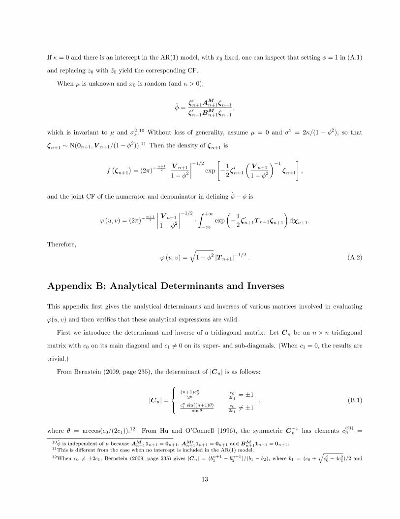
Appendix B: Analytical Determinants and Inverses
This appendix first gives the analytical determinants and inverses of various matrices involved in evaluating
ϕ(u, v) and then verifies that these analytical expressions are valid.
First we introduce the determinant and inverse of a tridiagonal matrix. Let Cn be an n × n tridiagonal
matrix with c0 on its main diagonal and c1 6= 0 on its super- and sub-diagonals. (When c1 = 0, the results are
trivial.)
From Bernstein (2009, page 235), the determinant of |Cn| is as follows:
|Cn| =
(n+1)cn0
2nc02c1
= ±1
cn1 sin((n+1)θ)sin θ
c02c16= ±1
, (B.1)
where θ = arccos(c0/(2c1)).12 From Hu and O’Connell (1996), the symmetric C−1n has elements c(ij)n =
10φ is independent of µ because AMn+11n+1 = 0n+1, AM ′
n+11n+1 = 0n+1 and BMn+11n+1 = 0n+1.
11This is different from the case when no intercept is included in the AR(1) model.
12When c0 6= ±2c1, Bernstein (2009, page 235) gives |Cn| = (bn+11 − bn+1
2 )/(b1 − b2), where b1 = (c0 +√c20 − 4c21)/2 and
13

(−1)i+j |Ci−1| |Cn−j | /(ci−j1 |Cn|) for i ≤ j. Substituting the determinant result (B.1) yields
c(ij)n =
2i(n−j+1)(n+1)c0
(− c0
2c1
)i−jc02c1
= ±1
(−1)i+j sin(iθ) sin((n−j+1)θ)c1 sin θ sin((n+1)θ)
c02c16= ±1
, i ≤ j, (B.2)
With the explicit expression of c(ij)n , we can derive the follow results:
ι′nC−1n ιn =
n(n+1)(n+2)
6c0c02c1
= −1
2n2+4n+1−(−1)n4c0(n+1)
c02c1
= 1
n+14c1 cos2(θ/2) −
tan2(θ/2)[(−1)n+cos((n+1)θ)]2c1 sin θ sin((n+1)θ)
c02c16= ±1
, (B.3)
e′1,nC−1n ιn =
nc0
c02c1
= −1
2n+1−(−1)n2c0(n+1)
c02c1
= 1
sin((2n+1)θ/2)−(−1)n sin(θ/2)2c1 sin((n+1)θ) cos(θ/2)
c02c16= ±1
, (B.4)
e′1,nC−1n e1,n =
2n
c0(n+1)c02c1
= ±1
sin(nθ)c1 sin((n+1)θ)
c02c16= ±1
, (B.5)
e′1,nC−1n en,n =
2(−c0/(2c1))n+1
c0(n+1)c02c1
= ±1
(−1)n+1 sin(θ)c1 sin((n+1)θ)
c02c16= ±1
. (B.6)
In the sequel, let c0 = 1 + φ2 + 2i(uφ − v), c1 = −(φ + iu), c2 = 2i(u + v − uφ), and c3 = i(2φu − 2v − u).
Since φ > 0, the case of c0 = 2c1, corresponding to φ = −1 and v = 0, is ruled out.
Determinant of Rn
Note that Rn is a tridiagonal matrix with its main diagonal elements rn,ii = c0, i = 1, · · · n − 1, rn,ii = 1,
i = n, and sub- and super-diagonal elements c1. Expanding along the last row of Rn leads to
|Rn| = |Cn−1| − c21 |Cn−2| , (B.7)
where the determinants of Cn−1 and Cn−2 follow from (B.1).
b2 = (c0 −√c20 − 4c21)/2. This can be numerically unstable when b1 is close to b2. Using polar representation, we write b1 =
c1 (cos θ + i sin θ) , b2 = c1 (cos θ − i sin θ). Then it follows that when c0 6= ±2c1, |Cn| = [cn1 sin((n + 1)θ)]/ sin θ. We thankRaymond Kan for pointing out this result and the results (B.3)–(B.6) to follow.
14
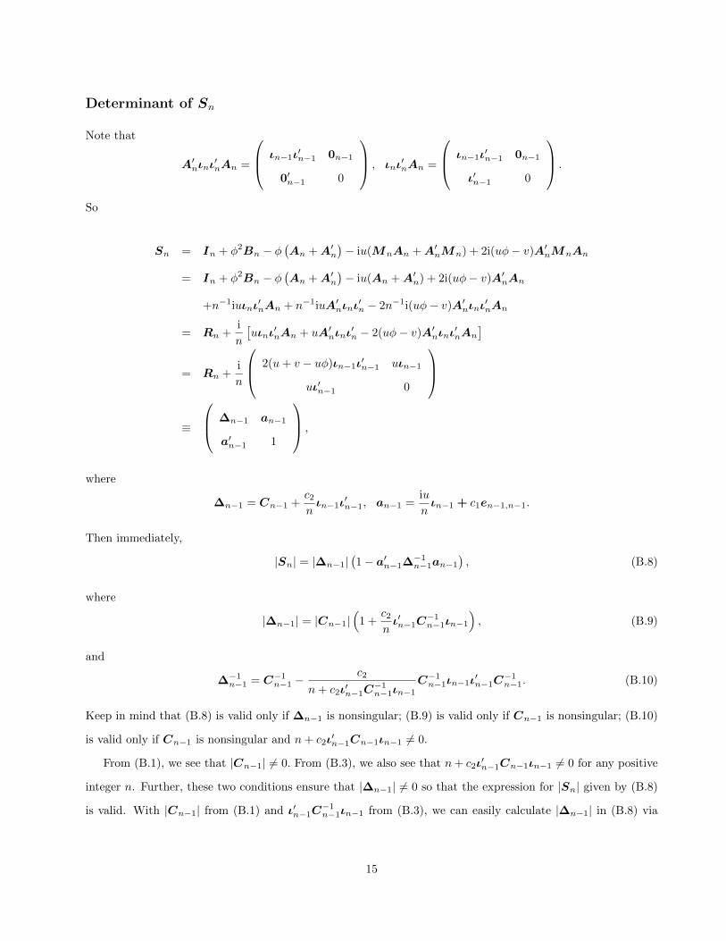
Determinant of Sn
Note that
A′nιnι′nAn =
ιn−1ι′n−1 0n−1
0′n−1 0
, ιnι′nAn =
ιn−1ι′n−1 0n−1
ι′n−1 0
.
So
Sn = In + φ2Bn − φ(An +A′n
)− iu(MnAn +A′nMn) + 2i(uφ− v)A′nMnAn
= In + φ2Bn − φ(An +A′n
)− iu(An +A′n) + 2i(uφ− v)A′nAn
+n−1iuιnι′nAn + n−1iuA′nιnι
′n − 2n−1i(uφ− v)A′nιnι
′nAn
= Rn +i
n
[uιnι
′nAn + uA′nιnι
′n − 2(uφ− v)A′nιnι
′nAn
]= Rn +
i
n
2(u+ v − uφ)ιn−1ι′n−1 uιn−1
uι′n−1 0
≡
∆n−1 an−1
a′n−1 1
,
where
∆n−1 = Cn−1 +c2nιn−1ι
′n−1, an−1 =
iu
nιn−1 + c1en−1,n−1.
Then immediately,
|Sn| = |∆n−1|(1− a′n−1∆
−1n−1an−1
), (B.8)
where
|∆n−1| = |Cn−1|(
1 +c2nι′n−1C
−1n−1ιn−1
), (B.9)
and
∆−1n−1 = C−1n−1 −c2
n+ c2ι′n−1C−1n−1ιn−1
C−1n−1ιn−1ι′n−1C
−1n−1. (B.10)
Keep in mind that (B.8) is valid only if ∆n−1 is nonsingular; (B.9) is valid only if Cn−1 is nonsingular; (B.10)
is valid only if Cn−1 is nonsingular and n+ c2ι′n−1Cn−1ιn−1 6= 0.
From (B.1), we see that |Cn−1| 6= 0. From (B.3), we also see that n+ c2ι′n−1Cn−1ιn−1 6= 0 for any positive
integer n. Further, these two conditions ensure that |∆n−1| 6= 0 so that the expression for |Sn| given by (B.8)
is valid. With |Cn−1| from (B.1) and ι′n−1C−1n−1ιn−1 from (B.3), we can easily calculate |∆n−1| in (B.8) via
15

(B.9). Note that the remaining term
a′n−1∆−1n−1an−1 = −u
2
n2ι′n−1C
−1n−1ιn−1 + c21e
′1,n−1C
−1n−1e1,n−1
+2ic1u
ne′1,n−1C
−1n−1ιn−1
− 2ic1c2u
n(n+ c2ι′n−1C−1n−1ιn−1)
ι′n−1C−1n−1ιn−1e
′1,n−1C
−1n−1ιn−1
+c2u
2
n2(n+ c2ι′n−1C−1n−1ιn−1)
(ι′n−1C−1n−1ιn−1)2
− c21c2
n+ c2ι′n−1C−1n−1ιn−1
(e′1,n−1C−1n−1ιn−1)2, (B.11)
where ι′n−1∆−1n−1ιn−1, e
′1,n−1C
−1n−1ιn−1, and e′1,n−1C
−1n−1e1,n−1 follow directly from (B.3), (B.4), and (B.5),
respectively.
Inverse of Sn
With ∆−1n−1 given by (B.10), the inverse of Sn is straightforward:
S−1n =
∆−1n−1 0n−1
0′n−1 0
+
∆−1n−1an−1
−1
( a′n−1∆−1n−1 −1
)1− a′n−1∆
−1n−1an−1
, (B.12)
if ∆n−1 is nonsingular and 1− a′n−1∆−1n−1an−1 6= 0. We have already showed that ∆n−1 is nonsingular. From
(B.11), we can verify that 1− a′n−1∆−1n−1an−1 6= 0 for any positive integer n.
Note that we need S−1n as δ′nS−1n δn appears in the CF (A.1). Given δn = iu(In − 2φA′n)Mne1,n +
2ivA′nMne1,n + φe1,n, we partition it as follows:
δn =
iu(e1,n−1 − 1nιn−1) + 2i(φu−v)
n ιn−1 + φe1,n−1
− iun
≡
δ1:n−1,n
− iun
.
16

So
δ′nS−1n δn = δ′n
∆−1n−1 0n−1
0′n−1 0
δn
+
δ′n
∆−1n−1an−1
−1
( a′n−1∆−1n−1 −1
)δn
1− a′n−1∆−1n−1an−1
= δ′1:n−1,n∆−1n−1δ1:n−1,n
+(δ′1:n−1,n∆−1n−1an−1)2 + 2iu
n δ′1:n−1,n∆−1n−1an−1 − u2
n2
1− a′n−1∆−1n−1an−1
, (B.13)
where a′n−1∆−1n−1an−1 follows from (B.11) and
δ′1:n−1,n∆−1n−1δ1:n−1,n =c23n2ι′n−1C
−1n−1ιn−1 +
2c1c3n
e′1,n−1C−1n−1ιn−1
+c21e′1,n−1C
−1n−1e1,n−1
− c2c23
n2(n+ c2ι′n−1C−1n−1ιn−1)
(ι′n−1C
−1n−1ιn−1
)2− c21c2
n+ c2ι′n−1C−1n−1ιn−1
(e′1,n−1C−1n−1ιn−1)2
− 2c1c2c3
n(n+ c2ι′n−1C−1n−1ιn−1)
e′1,n−1C−1n−1ιn−1ι
′n−1C
−1n−1ιn−1, (B.14)
δ′1:n−1,n∆−1n−1an−1 =iuc3n2ι′n−1C
−1n−1ιn−1 − c21e′1,n−1C
−1n−1en−1,n−1
−c1c2ne′1,n−1C
−1n−1ιn−1
+c21c2
n+ c2ι′n−1C−1n−1ιn−1
(e′1,n−1C−1n−1ιn−1)2
− iuc2c3
n2(n+ c2ι′n−1C−1n−1ιn−1)
(ι′n−1C−1n−1ιn−1)2
+c1c
22
n(n+ c2ι′n−1C−1n−1ιn−1)
e′1,n−1C−1n−1ιn−1ι
′n−1C
−1n−1ιn−1. (B.15)
which can be calculated by substituting (B.3)–(B.6).
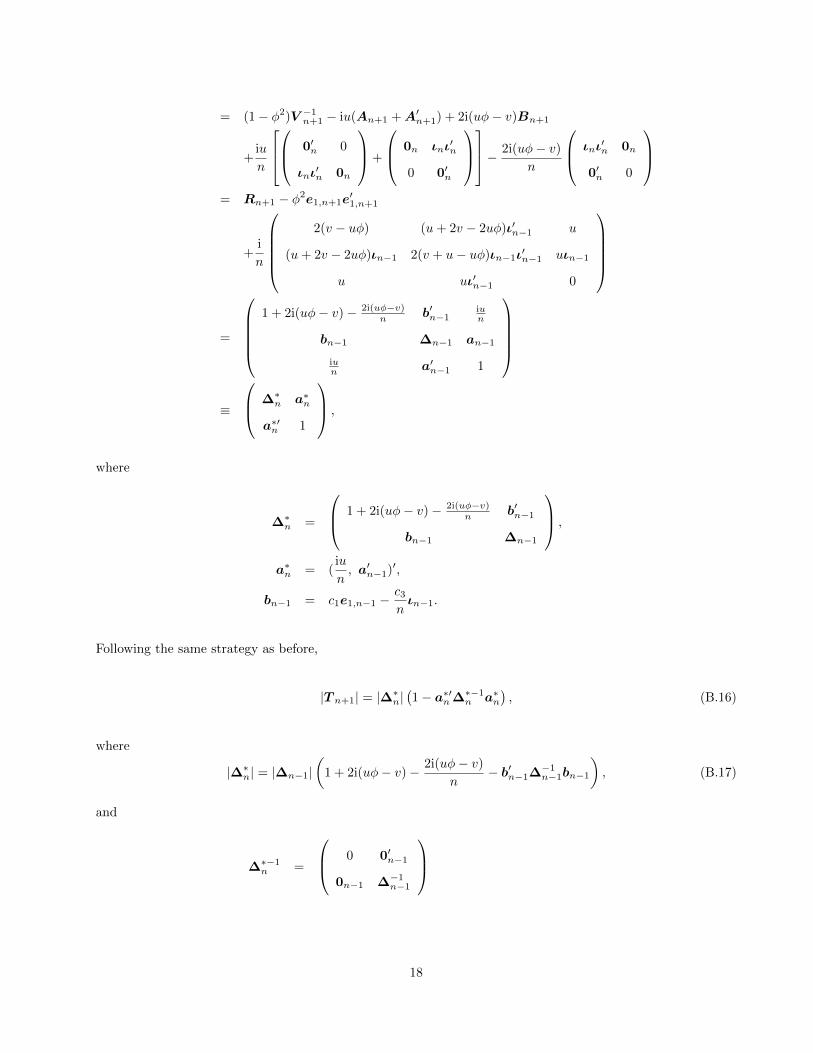
Determinant of T n+1
Note that
T n+1 = (1− φ2)V −1n+1 − iu(AMn+1 +AM ′
n+1) + 2i(uφ− v)BMn+1
17
= (1− φ2)V −1n+1 − iu(An+1 +A′n+1) + 2i(uφ− v)Bn+1
+iu
n
0′n 0
ιnι′n 0n
+
0n ιnι′n
0 0′n
− 2i(uφ− v)
n
ιnι′n 0n
0′n 0
= Rn+1 − φ2e1,n+1e
′1,n+1
+i
n
2(v − uφ) (u+ 2v − 2uφ)ι′n−1 u
(u+ 2v − 2uφ)ιn−1 2(v + u− uφ)ιn−1ι′n−1 uιn−1
u uι′n−1 0
=
1 + 2i(uφ− v)− 2i(uφ−v)
n b′n−1iun
bn−1 ∆n−1 an−1
iun a′n−1 1
≡
∆∗n a∗n
a∗′n 1
,
where
∆∗n =
1 + 2i(uφ− v)− 2i(uφ−v)n b′n−1
bn−1 ∆n−1
,
a∗n = (iu
n, a′n−1)′,
bn−1 = c1e1,n−1 −c3nιn−1.
Following the same strategy as before,
|T n+1| = |∆∗n|(1− a∗′n∆∗−1n a∗n
), (B.16)
where
|∆∗n| = |∆n−1|(
1 + 2i(uφ− v)− 2i(uφ− v)
n− b′n−1∆
−1n−1bn−1
), (B.17)
and
∆∗−1n =
0 0′n−1
0n−1 ∆−1n−1
18

+
−1
∆−1n−1bn−1
( −1 b′n−1∆−1n−1
)1 + 2i(uφ− v)− 2i(uφ−v)
n − b′n−1∆−1n−1bn−1
. (B.18)
For (B.16) to be valid, ∆∗n needs to be nonsingular; for (B.17) to be valid, ∆n−1 needs to be nonsingular;
for (B.18) to be valid, ∆n−1 needs to be nonsingular and 1 + 2i(uφ− v)− 2i(uφ− v)/n− b′n−1∆−1n−1bn−1 6= 0.
We have already shown that ∆n−1 is nonsingular. Note that
b′n−1∆−1n−1bn−1 =
c23n2ι′n−1C
−1n−1ιn−1 −
2c1c3n
e′1,n−1C−1n−1ιn−1
+c21e′1,n−1C
−1n−1e1,n−1
− c2c23
n2(n+ c2ι′n−1C−1n−1ιn−1)
(ι′n−1C−1n−1ιn−1)2
− c21c2
n+ c2ι′n−1C−1n−1ιn−1
(e′1,n−1C−1n−1ιn−1)2
+2c1c2c3
n(n+ c2ι′n−1C−1n−1ιn−1)
e′1,n−1C−1n−1ιn−1ι
′n−1C
−1n−1ιn−1, (B.19)
which can be evaluated with analytical expressions from (B.3)–(B.5), and we can verify that 1 + 2i(uφ − v) −
2i(uφ− v)/n− b′n−1∆−1n−1bn−1 6= 0 for any positive integer n.
For us to use (B.16), we still need expression for a∗′n∆∗−1n a∗n. By substitution,
a∗′n∆∗−1n a∗n = a′n−1∆−1n−1an−1
+−u2 − 2inua′n−1∆
−1n−1bn−1 + n2(a′n−1∆
−1n−1bn−1)2
n2 + 2in2(uφ− v)− 2in(uφ− v)− n2b′n−1∆−1n−1bn−1
, (B.20)
where a′n−1∆−1n−1an−1 is given by (B.11), b′n−1∆
−1n−1bn−1 is given by (B.19), and
a′n−1∆−1n−1bn−1 = − iuc3
n2ι′n−1C
−1n−1ιn−1 +
c1c2ne′1,n−1C
−1n−1ιn−1
+c21e′1,n−1C
−1n−1en−1,n−1
+iuc2c3
n2(n+ c2ι′n−1C−1n−1ιn−1)
(ι′n−1C−1n−1ιn−1)2
− c21c2
n+ c2ι′n−1C−1n−1ιn−1
(e′1,n−1C−1n−1ιn−1)2
− c1c22
n(n+ c2ι′n−1C−1n−1ιn−1)
e′1,n−1C−1n−1ιn−1ι
′n−1C
−1n−1ιn−1, (B.21)
which can be evaluated with analytical expressions from (B.3)–(B.6).
19

Appendix C: Numerical Integration
Given the characteristic functions in Section 2.1, we need to implement numerical integration to calculate (2.6)
via (2.7). This can be straightforwardly implemented using Matlab’s quadgk command. One caveat to note
is that the square root function in the complex domain is not continuous. One choice is to follow Perron
(1989) to identify explicitly the discontinuous points by grid search and then integrate by parts. The search,
however, might be inefficient and time-consuming. Instead, we use the following algorithm so that the integrand
function for quadgk is always continuous. Let g (t) =√a(t) + ib(t) denote the integrand function in question
with t ∈ [l, u] . quadgk requires the integrand function to accept a vector (t1, t2, · · · , tn) and returns a vector of
output. Let θi = arg (a(ti) + ib(ti)) ∈ [−π, π] and denote ai = a (ti) , bi = b (ti) , and gi = g (ti) .
1. Start with t1 and set g1 = sqrt (a1 + ib1) . Set k = 0.
2. Beginning with t2, if ai < 0, ai−1 < 0, and bibi−1 <= 0, set k = k + 1; otherwise, k is unchanged. Set
gi =√a2i + b2i (cos (θ∗i /2) + i sin (θ∗i /2)) , where θ∗i = θi + 2kπ.
20
Tab
le1,
Pan
elA
(T=
1):
Pr(T
(κ−κ
)≤w
),F
ixed
x0,κ
=0.
01,x0
=µ
=0,σ
=0.
1
Month
lyD
ail
yw
ppedf
pexp
pmix
pinf
ppedf
pexp
pmix
pinf
-50.
0002
0.00
02
0.0
000
0.0
000
0.0
000
0.0
001
0.0
000
0.0
000
0.0
000
0.0
000
-30.
0037
0.00
36
0.0
000
0.0
000
0.0
013
0.0
013
0.0
013
0.0
000
0.0
000
0.0
014
-20.
0201
0.02
02
0.0
000
0.0
000
0.0
109
0.0
110
0.0
112
0.0
000
0.0
000
0.0
105
-1.5
0.04
870.
0485
0.0
000
0.0
000
0.0
317
0.0
323
0.0
326
0.0
000
0.0000
0.0
310
-10.
1126
0.11
29
0.0
000
0.0
000
0.0
884
0.0
892
0.0
888
0.0
000
0.0
000
0.0
876
-0.8
0.15
110.
1515
0.0
000
0.0
000
0.1
249
0.1
261
0.1
253
0.0
000
0.0000
0.1
245
-0.6
0.19
580.
1963
0.0
000
0.0
000
0.1
679
0.1
691
0.1
697
0.0
000
0.0000
0.1
688
-0.4
0.24
390.
2444
0.0
023
0.0
023
0.2
173
0.2
190
0.2
186
0.0
023
0.0023
0.2
171
-0.2
0.29
280.
2931
0.0
787
0.0
786
0.2
682
0.2
688
0.2
686
0.0
787
0.0786
0.2
682
-0.1
0.31
690.
3174
0.2
398
0.2
398
0.2
933
0.2
946
0.2
932
0.2
398
0.2398
0.2
934
-0.0
10.
3380
0.33
84
0.4
718
0.4
718
0.3
153
0.3
154
0.3
153
0.4
718
0.4
718
0.3
157
-0.0
010.
3401
0.34
05
0.4
972
0.4
972
0.3
175
0.3
180
0.3
175
0.4
972
0.4972
0.3
179
00.
3403
0.34
08
0.5
000
0.5
000
0.3
177
0.3
183
0.3
177
0.5
000
0.5
000
0.3
181
0.00
10.
3406
0.34
10
0.5
028
0.5
028
0.3
180
0.3
185
0.3
180
0.5
028
0.5
028
0.3
184
0.01
0.34
270.
3432
0.5
282
0.5
282
0.3
202
0.3
207
0.3
202
0.5
282
0.5282
0.3
203
0.1
0.36
320.
3638
0.7
602
0.7
602
0.3
411
0.3
421
0.3
414
0.7
602
0.7
602
0.3
414
0.2
0.38
530.
3856
0.9
213
0.9
214
0.3
644
0.3
651
0.3
644
0.9
213
0.9
214
0.3
649
0.4
0.42
710.
4271
0.9
977
0.9
977
0.4
081
0.4
095
0.4
088
0.9
977
0.9
977
0.4
086
0.6
0.46
600.
4660
1.0
000
1.0
000
0.4
492
0.4
512
0.4
507
1.0
000
1.0
000
0.4
516
0.8
0.50
240.
5026
1.0
000
1.0
000
0.4
889
0.4
904
0.4
899
1.0
000
1.0
000
0.4
907
10.
5366
0.53
72
1.0
000
1.0
000
0.5
255
0.5
267
0.5
263
1.0
000
1.0000
0.5
273
1.5
0.61
110.
6115
1.0
000
1.0
000
0.6
050
0.6
053
0.6
051
1.0
000
1.0
000
0.6
055
20.
6711
0.67
13
1.0
000
1.0
000
0.6
700
0.6
691
0.6
687
1.0
000
1.0000
0.6
695
30.
7592
0.75
94
1.0
000
1.0
000
0.7
628
0.7
638
0.7
634
1.0
000
1.0000
0.7
647
50.
8617
0.86
18
1.0
000
1.0
000
0.8
757
0.8
746
0.8
742
1.0
000
1.0000
0.8
755
80.
9318
0.93
18
1.0
000
1.0
000
0.9
490
0.9
485
0.9
484
1.0
000
1.0000
0.9
498
200.
9906
0.99
04
1.0
000
1.0
000
0.9
980
0.9
980
0.9
981
1.0
000
1.0
000
0.9
982
500.
9995
0.99
95
1.0
000
1.0
000
1.0
000
1.0
000
1.0
000
1.0
000
1.0
000
1.0
000
100
1.00
001.
0000
1.0
000
1.0
000
1.0
000
1.0
000
1.0
000
1.0
000
1.0000
1.0
000
21

Tab
le1,
Panel
B(T
=10):
Pr(T
(κ−κ
)≤w
),F
ixed
x0,κ
=0.
01,x0
=µ
=0,σ
=0.
1
Month
lyD
ail
yw
ppedf
pexp
pmix
pinf
ppedf
pexp
pmix
pinf
-50.
0000
0.00
00
0.1
319
0.1
318
0.0
000
0.0
000
0.0
000
0.1
318
0.1
318
0.0
000
-30.
0015
0.00
15
0.2
513
0.2
512
0.0
014
0.0
013
0.0
013
0.2
512
0.2
512
0.0
014
-20.
0124
0.01
24
0.3
274
0.3
274
0.0
114
0.0
116
0.0
115
0.3
274
0.3
274
0.0
120
-1.5
0.03
550.
0356
0.3
687
0.3
687
0.0
347
0.0
341
0.0
342
0.3
687
0.3687
0.0
348
-10.
0940
0.09
38
0.4
116
0.4
115
0.0
924
0.0
918
0.0
919
0.4
115
0.4
115
0.0
929
-0.8
0.13
100.
1308
0.4
290
0.4
290
0.1
291
0.1
288
0.1
289
0.4
290
0.4290
0.1
284
-0.6
0.17
490.
1745
0.4
467
0.4
466
0.1
734
0.1
725
0.1
729
0.4
466
0.4466
0.1
715
-0.4
0.22
260.
2221
0.4
644
0.4
644
0.2
207
0.2
194
0.2
206
0.4
644
0.4644
0.2
192
-0.2
0.27
150.
2710
0.4
822
0.4
822
0.2
703
0.2
677
0.2
698
0.4
822
0.4822
0.2
694
-0.1
0.29
570.
2952
0.4
911
0.4
911
0.2
958
0.2
928
0.2
941
0.4
911
0.4911
0.2
935
-0.0
10.
3171
0.31
66
0.4
991
0.4
991
0.3
169
0.3
152
0.3
155
0.4
991
0.4
991
0.3
153
-0.0
010.
3192
0.31
88
0.4
999
0.4
999
0.3
191
0.3
163
0.3
176
0.4
999
0.4999
0.3
175
00.
3194
0.31
90
0.5
000
0.5
000
0.3
194
0.3
166
0.3
178
0.5
000
0.5
000
0.3
177
0.00
10.
3197
0.31
93
0.5
001
0.5
001
0.3
195
0.3
168
0.3
181
0.5
001
0.5
001
0.3
179
0.01
0.32
180.
3213
0.5
009
0.5
009
0.3
216
0.3
190
0.3
201
0.5
009
0.5009
0.3
199
0.1
0.34
270.
3422
0.5
089
0.5
089
0.3
424
0.3
404
0.3
410
0.5
089
0.5
089
0.3
415
0.2
0.36
540.
3647
0.5
178
0.5
178
0.3
655
0.3
637
0.3
639
0.5
178
0.5
178
0.3
641
0.4
0.41
070.
4082
0.5
356
0.5
356
0.4
101
0.4
077
0.4
077
0.5
356
0.5
356
0.4
077
0.6
0.45
050.
4494
0.5
533
0.5
534
0.4
518
0.4
493
0.4
493
0.5
534
0.5
534
0.4
500
0.8
0.48
920.
4882
0.5
710
0.5
710
0.4
904
0.4
883
0.4
882
0.5
710
0.5
710
0.4
891
10.
5204
0.52
39
0.5
884
0.5
885
0.5
264
0.5
244
0.5
244
0.5
885
0.5885
0.5
252
1.5
0.60
300.
6017
0.6
313
0.6
313
0.6
059
0.6
027
0.6
033
0.6
313
0.6
313
0.6
044
20.
6663
0.66
53
0.6
726
0.6
726
0.6
683
0.6
664
0.6
674
0.6
726
0.6726
0.6
681
30.
7607
0.76
02
0.7
487
0.7
488
0.7
636
0.7
616
0.7
627
0.7
488
0.7488
0.7
629
50.
8720
0.87
17
0.8
681
0.8
682
0.8
735
0.8
735
0.8
740
0.8
682
0.8682
0.8
739
80.
9467
0.94
68
0.9
631
0.9
632
0.9
484
0.9
484
0.9
487
0.9
632
0.9632
0.9
489
200.
9977
0.99
77
1.0
000
1.0
000
0.9
981
0.9
982
0.9
981
1.0
000
1.0
000
0.9
982
501.
0000
1.00
00
1.0
000
1.0
000
1.0
000
1.0
000
1.0
000
1.0
000
1.0
000
1.0
000
100
1.00
001.
0000
1.0
000
1.0
000
1.0
000
1.0
000
1.0
000
1.0
000
1.0000
1.0
000
22

Tab
le2,
Pan
elA
(T=
1):
Pr(T
(κ−κ
)≤w
),F
ixed
x0,κ
=0.
01,x0
=µ
=0.
1,σ
=0.
1
Month
lyD
ail
yw
ppedf
pexp
pmix
pinf
ppedf
pexp
pmix
pinf
-50.
0001
0.00
01
0.0
000
0.0
000
0.0
000
0.0
001
0.0
000
0.0
000
0.0
000
0.0
000
-30.
0016
0.00
16
0.0
000
0.0
000
0.0
003
0.0
004
0.0
004
0.0
000
0.0
000
0.0
004
-20.
0060
0.00
60
0.0
000
0.0
000
0.0
021
0.0
020
0.0
022
0.0
000
0.0
000
0.0
021
-1.5
0.01
140.
0114
0.0
000
0.0
000
0.0
049
0.0
045
0.0
051
0.0
000
0.0000
0.0
049
-10.
0209
0.02
09
0.0
000
0.0
000
0.0
108
0.0
113
0.0
112
0.0
000
0.0
000
0.0
108
-0.8
0.02
630.
0264
0.0
000
0.0
000
0.0
146
0.0
152
0.0
151
0.0
000
0.0000
0.0
144
-0.6
0.03
290.
0330
0.0
000
0.0
000
0.0
194
0.0
188
0.0
199
0.0
000
0.0000
0.0
192
-0.4
0.04
080.
0409
0.0
023
0.0
023
0.0
258
0.0
263
0.0
262
0.0
023
0.0023
0.0
251
-0.2
0.05
010.
0501
0.0
787
0.0
787
0.0
332
0.0
339
0.0
339
0.0
787
0.0787
0.0
324
-0.1
0.05
530.
0554
0.2
398
0.2
398
0.0
373
0.0
379
0.0
383
0.2
398
0.2398
0.0
369
-0.0
10.
0603
0.06
03
0.4
718
0.4
718
0.0
417
0.0
425
0.0
425
0.4
718
0.4
718
0.0
412
-0.0
010.
0609
0.06
08
0.4
972
0.4
972
0.0
421
0.0
429
0.0
430
0.4
972
0.4972
0.0
418
00.
0609
0.06
09
0.5
000
0.5
000
0.0
422
0.0
430
0.0
430
0.5
000
0.5
000
0.0
418
0.00
10.
0610
0.06
09
0.5
028
0.5
028
0.0
423
0.0
430
0.0
431
0.5
028
0.5
028
0.0
419
0.01
0.06
150.
0615
0.5
282
0.5
282
0.0
427
0.0
435
0.0
436
0.5
282
0.5282
0.0
423
0.1
0.06
690.
0669
0.7
602
0.7
603
0.0
474
0.0
484
0.0
483
0.7
603
0.7
603
0.0
470
0.2
0.07
320.
0732
0.9
213
0.9
214
0.0
532
0.0
541
0.0
539
0.9
214
0.9
214
0.0
525
0.4
0.08
710.
0869
0.9
977
0.9
977
0.0
655
0.0
665
0.0
665
0.9
977
0.9
977
0.0
649
0.6
0.10
230.
1021
1.0
000
1.0
000
0.0
798
0.0
809
0.0
809
1.0
000
1.0
000
0.0
791
0.8
0.11
900.
1187
1.0
000
1.0
000
0.0
952
0.0
399
0.0
967
1.0
000
1.0
000
0.0
950
10.
1368
0.13
66
1.0
000
1.0
000
0.1
130
0.1
145
0.1
143
1.0
000
1.0000
0.1
125
1.5
0.18
540.
1851
1.0
000
1.0
000
0.1
620
0.1
643
0.1
641
1.0
000
1.0
000
0.1
635
20.
2380
0.23
80
1.0
000
1.0
000
0.2
187
0.2
207
0.2
206
1.0
000
1.0000
0.2
186
30.
3477
0.34
75
1.0
000
1.0
000
0.3
423
0.3
423
0.3
419
1.0
000
1.0000
0.3
410
50.
5460
0.54
56
1.0
000
1.0
000
0.5
641
0.5
634
0.5
629
1.0
000
1.0000
0.5
658
80.
7392
0.73
86
1.0
000
1.0
000
0.7
840
0.7
792
0.7
787
1.0
000
1.0000
0.7
812
200.
9562
0.95
62
1.0
000
1.0
000
0.9
879
0.9
873
0.9
872
1.0
000
1.0
000
0.9
877
500.
9977
0.99
77
1.0
000
1.0
000
1.0
000
1.0
000
1.0
000
1.0
000
1.0
000
1.0
000
100
1.00
001.
0000
1.0
000
1.0
000
1.0
000
1.0
000
1.0
000
1.0
000
1.0000
1.0
000
23
Tab
le2,
Pan
elB
(T=
10):
Pr(T
(κ−κ
)≤w
),F
ixed
x0,κ
=0.
01,x0
=µ
=0.
1,σ
=0.
1
Month
lyD
ail
yw
ppedf
pexp
pmix
pinf
ppedf
pexp
pmix
pinf
-50.
0000
0.00
00
0.1
319
0.1
318
0.0
000
0.0
000
0.0
000
0.1
318
0.1
318
0.0
000
-30.
0005
0.00
05
0.2
513
0.2
512
0.0
004
0.0
004
0.0
004
0.2
512
0.2
512
0.0
004
-20.
0025
0.00
26
0.3
274
0.3
274
0.0
023
0.0
022
0.0
022
0.3
274
0.3
274
0.0
024
-1.5
0.00
560.
0058
0.3
687
0.3
687
0.0
052
0.0
052
0.0
051
0.3
687
0.3687
0.0
054
-10.
0121
0.01
24
0.4
116
0.4
115
0.0
115
0.0
114
0.0
114
0.4
115
0.4
115
0.0
120
-0.8
0.01
600.
0165
0.4
290
0.4
290
0.0
152
0.0
153
0.0
152
0.4
290
0.4290
0.0
158
-0.6
0.02
130.
0215
0.4
467
0.4
466
0.0
199
0.0
202
0.0
203
0.4
466
0.4466
0.0
210
-0.4
0.02
760.
0279
0.4
644
0.4
644
0.0
260
0.0
257
0.0
265
0.4
644
0.4644
0.0
274
-0.2
0.03
540.
0357
0.4
822
0.4
822
0.0
333
0.0
341
0.0
341
0.4
822
0.4822
0.0
351
-0.1
0.03
980.
0401
0.4
911
0.4
911
0.0
376
0.0
384
0.0
385
0.4
911
0.4911
0.0
393
-0.0
10.
0441
0.04
45
0.4
991
0.4
991
0.0
420
0.0
425
0.0
426
0.4
991
0.4
991
0.0
436
-0.0
010.
0446
0.04
49
0.4
999
0.4
999
0.0
424
0.0
430
0.0
431
0.4
999
0.4999
0.0
442
00.
0446
0.04
50
0.5
000
0.5
000
0.0
425
0.0
430
0.0
432
0.5
000
0.5
000
0.0
443
0.00
10.
0447
0.04
50
0.5
001
0.5
001
0.0
426
0.0
431
0.0
432
0.5
001
0.5
001
0.0
444
0.01
0.04
510.
0455
0.5
009
0.5
009
0.0
430
0.0
434
0.0
437
0.5
009
0.5009
0.0
447
0.1
0.04
990.
0503
0.5
089
0.5
089
0.0
475
0.0
484
0.0
484
0.5
089
0.5
089
0.0
492
0.2
0.05
550.
0560
0.5
178
0.5
178
0.0
534
0.0
540
0.0
540
0.5
178
0.5
178
0.0
547
0.4
0.06
800.
0685
0.5
356
0.5
356
0.0
662
0.0
664
0.0
665
0.5
356
0.5
356
0.0
671
0.6
0.08
220.
0829
0.5
533
0.5
534
0.0
797
0.0
805
0.0
807
0.5
534
0.5
534
0.0
819
0.8
0.09
790.
0988
0.5
710
0.5
710
0.0
954
0.0
962
0.0
965
0.5
710
0.5
710
0.0
978
10.
1151
0.11
62
0.5
884
0.5
885
0.1
123
0.1
135
0.1
137
0.5
885
0.5885
0.1
148
1.5
0.16
400.
1651
0.6
313
0.6
313
0.1
613
0.1
627
0.1
629
0.6
313
0.6
313
0.1
632
20.
2195
0.22
07
0.6
726
0.6
726
0.2
175
0.2
186
0.2
190
0.6
726
0.6726
0.2
172
30.
3394
0.34
06
0.7
487
0.7
488
0.3
393
0.3
398
0.3
398
0.7
488
0.7488
0.3
383
50.
5585
0.55
97
0.8
681
0.8
682
0.5
624
0.5
613
0.5
613
0.8
682
0.8682
0.5
584
80.
7740
0.77
42
0.9
631
0.9
632
0.7
822
0.7
789
0.7
796
0.9
632
0.9632
0.7
781
200.
9857
0.98
56
1.0
000
1.0
000
0.9
884
0.9
880
0.9
881
1.0
000
1.0
000
0.9
885
501.
0000
1.00
00
1.0
000
1.0
000
1.0
000
1.0
000
1.0
000
1.0
000
1.0
000
1.0
000
100
1.00
001.
0000
1.0
000
1.0
000
1.0
000
1.0
000
1.0
000
1.0
000
1.0000
1.0
000
24
Tab
le3,
Pan
elA
(T=
1):
Pr(T
(κ−κ
)≤w
),R
an
domx0,κ
=0.
01,µ
=0,σ
=0.
1
Month
lyD
ail
yw
ppedf
pexp
pmix
pinf
ppedf
pexp
pmix
pinf
-50.
0000
0.00
00
0.0
000
0.0
000
0.0
099
0.0
000
0.0
000
0.0
000
0.0
000
0.0
099
-30.
0001
0.00
01
0.0
000
0.0
000
0.0
158
0.0
001
0.0
001
0.0
000
0.0
000
0.0
155
-20.
0008
0.00
09
0.0
000
0.0
000
0.0
210
0.0
005
0.0
005
0.0
000
0.0
000
0.0
203
-1.5
0.00
250.
0025
0.0
000
0.0
000
0.0
250
0.0
018
0.0
018
0.0
000
0.0000
0.0
242
-10.
0084
0.00
84
0.0
000
0.0
000
0.0
339
0.0
071
0.0
070
0.0
000
0.0
000
0.0
328
-0.8
0.01
440.
0145
0.0
000
0.0
000
0.0
423
0.0
127
0.0
127
0.0
000
0.0000
0.0
412
-0.6
0.02
640.
0265
0.0
000
0.0
000
0.0
581
0.0
241
0.0
242
0.0
000
0.0000
0.0
580
-0.4
0.05
360.
0536
0.0
023
0.0
023
0.0
919
0.0
506
0.0
508
0.0
023
0.0023
0.0
892
-0.2
0.13
430.
1340
0.0
787
0.0
787
0.1
715
0.1
302
0.1
297
0.0
787
0.0787
0.1
651
-0.1
0.24
300.
2432
0.2
398
0.2
398
0.2
658
0.2
382
0.2
378
0.2
398
0.2398
0.2
613
-0.0
10.
4202
0.42
08
0.4
718
0.4
718
0.4
232
0.4
152
0.4
145
0.4
718
0.4
718
0.4
227
-0.0
010.
4406
0.44
11
0.4
972
0.4
972
0.4
427
0.4
355
0.4
348
0.4
972
0.4972
0.4
427
00.
4428
0.44
34
0.5
000
0.5
000
0.4
449
0.4
377
0.4
370
0.5
000
0.5
000
0.4
450
0.00
10.
4451
0.44
56
0.5
028
0.5
028
0.4
471
0.4
400
0.4
393
0.5
028
0.5
028
0.4
472
0.01
0.46
530.
4658
0.5
282
0.5
282
0.4
669
0.4
602
0.4
596
0.5
282
0.5282
0.4
676
0.1
0.63
610.
6365
0.7
602
0.7
603
0.6
472
0.6
315
0.6
310
0.7
603
0.7
603
0.6
526
0.2
0.74
450.
7454
0.9
213
0.9
214
0.7
733
0.7
404
0.7
403
0.9
214
0.9
214
0.7
814
0.4
0.83
900.
8394
0.9
977
0.9
977
0.8
816
0.8
360
0.8
360
0.9
977
0.9
977
0.8
822
0.6
0.88
030.
8807
1.0
000
1.0
000
0.9
218
0.8
781
0.8
780
1.0
000
1.0
000
0.9
199
0.8
0.90
410.
9045
1.0
000
1.0
000
0.9
414
0.9
025
0.9
024
1.0
000
1.0
000
0.9
405
10.
9200
0.92
05
1.0
000
1.0
000
0.9
530
0.9
189
0.9
189
1.0
000
1.0000
0.9
526
1.5
0.94
460.
9451
1.0
000
1.0
000
0.9
684
0.9
441
0.9
443
1.0
000
1.0
000
0.9
676
20.
9590
0.95
93
1.0
000
1.0
000
0.9
760
0.9
590
0.9
591
1.0
000
1.0000
0.9
748
30.
9750
0.97
51
1.0
000
1.0
000
0.9
837
0.9
756
0.9
757
1.0
000
1.0000
0.9
826
50.
9886
0.98
86
1.0
000
1.0
000
0.9
901
0.9
897
0.9
897
1.0
000
1.0000
0.9
895
80.
9954
0.99
52
1.0
000
1.0
000
0.9
937
0.9
966
0.9
965
1.0
000
1.0000
0.9
935
200.
9995
0.99
95
1.0
000
1.0
000
0.9
975
0.9
999
0.9
999
1.0
000
1.0
000
0.9
974
501.
0000
1.00
00
1.0
000
1.0
000
0.9
990
1.0
000
1.0
000
1.0
000
1.0
000
0.9
990
100
1.00
001.
0000
1.0
000
1.0
000
0.9
995
1.0
000
1.0
000
1.0
000
1.0000
0.9
995
25
Tab
le3,
Pan
elB
(T=
10):
Pr(T
(κ−κ
)≤w
),R
an
domx0,κ
=0.
01,µ
=0,σ
=0.
1
Month
lyD
ail
yw
ppedf
pexp
pmix
pinf
ppedf
pexp
pmix
pinf
-50.
0000
0.00
00
0.1
319
0.1
318
0.0
265
0.0
000
0.0
000
0.1
318
0.1
318
0.0
260
-30.
0002
0.00
02
0.2
513
0.2
512
0.0
418
0.0
002
0.0
001
0.2
512
0.2
512
0.0
407
-20.
0019
0.00
19
0.3
274
0.3
274
0.0
548
0.0
019
0.0
017
0.3
274
0.3
274
0.0
527
-1.5
0.00
630.
0065
0.3
687
0.3
687
0.0
639
0.0
062
0.0
062
0.3
687
0.3687
0.0
611
-10.
0235
0.02
37
0.4
116
0.4
115
0.0
850
0.0
231
0.0
230
0.4
115
0.4
115
0.0
811
-0.8
0.04
110.
0410
0.4
290
0.4
290
0.1
053
0.0
405
0.0
406
0.4
290
0.4290
0.1
013
-0.6
0.07
360.
0731
0.4
467
0.4
466
0.1
432
0.0
729
0.0
729
0.4
466
0.4466
0.1
404
-0.4
0.13
420.
1338
0.4
644
0.4
644
0.2
081
0.1
334
0.1
332
0.4
644
0.4644
0.2
077
-0.2
0.23
940.
2393
0.4
822
0.4
822
0.2
931
0.2
385
0.2
385
0.4
822
0.4822
0.2
944
-0.1
0.31
020.
3084
0.4
911
0.4
911
0.3
441
0.3
073
0.3
076
0.4
911
0.4911
0.3
458
-0.0
10.
3760
0.37
40
0.4
991
0.4
991
0.3
991
0.3
730
0.3
730
0.4
991
0.4
991
0.4
016
-0.0
010.
3805
0.38
04
0.4
999
0.4
999
0.4
052
0.3
795
0.3
797
0.4
999
0.4999
0.4
077
00.
3812
0.38
12
0.5
000
0.5
000
0.4
059
0.3
803
0.3
804
0.5
000
0.5
000
0.4
084
0.00
10.
3819
0.38
19
0.5
001
0.5
001
0.4
065
0.3
810
0.3
811
0.5
001
0.5
001
0.4
091
0.01
0.38
850.
3884
0.5
009
0.5
009
0.4
127
0.3
875
0.3
878
0.5
009
0.5009
0.4
153
0.1
0.45
120.
4510
0.5
089
0.5
089
0.4
779
0.4
502
0.4
505
0.5
089
0.5
089
0.4
813
0.2
0.51
350.
5134
0.5
178
0.5
178
0.5
553
0.5
126
0.5
132
0.5
178
0.5
178
0.5
588
0.4
0.61
130.
6108
0.5
356
0.5
356
0.7
052
0.6
106
0.6
111
0.5
356
0.5
356
0.7
094
0.6
0.68
040.
6803
0.5
533
0.5
534
0.7
949
0.6
799
0.6
801
0.5
534
0.5
534
0.7
980
0.8
0.73
090.
7308
0.5
710
0.5
710
0.8
479
0.7
305
0.7
311
0.5
710
0.5
710
0.8
509
10.
7694
0.76
93
0.5
884
0.5
885
0.8
805
0.7
691
0.7
695
0.5
885
0.5885
0.8
821
1.5
0.83
490.
8349
0.6
313
0.6
313
0.9
208
0.8
348
0.8
349
0.6
313
0.6
313
0.9
206
20.
8763
0.87
59
0.6
726
0.6
726
0.9
393
0.8
763
0.8
765
0.6
726
0.6726
0.9
389
30.
9249
0.92
49
0.7
487
0.7
488
0.9
585
0.9
251
0.9
251
0.7
488
0.7488
0.9
576
50.
9677
0.96
76
0.8
681
0.8
682
0.9
744
0.9
680
0.9
680
0.8
682
0.8682
0.9
738
80.
9891
0.98
90
0.9
631
0.9
632
0.9
838
0.9
894
0.9
896
0.9
632
0.9632
0.9
834
200.
9997
0.99
97
1.0
000
1.0
000
0.9
934
0.9
998
0.9
998
1.0
000
1.0
000
0.9
933
501.
0000
1.00
00
1.0
000
1.0
000
0.9
973
1.0
000
1.0
000
1.0
000
1.0
000
0.9
973
100
1.00
001.
0000
1.0
000
1.0
000
0.9
987
1.0
000
1.0
000
1.0
000
1.0000
0.9
987
26

Tab
le4,
Pan
elA
(T=
1):
Pr(T
(κ−κ
)≤w
),R
an
domx0,κ
=0.
01,µ
=0.
1,σ
=0.
1
Month
lyD
ail
yw
ppedf
pexp
pmix
pinf
ppedf
pexp
pmix
pinf
-50.
0001
0.00
01
0.0
000
0.0
000
0.0
000
0.0
001
0.0
000
0.0
000
0.0
000
0.0
000
-30.
0016
0.00
16
0.0
000
0.0
000
0.0
003
0.0
004
0.0
004
0.0
000
0.0
000
0.0
003
-20.
0061
0.00
60
0.0
000
0.0
000
0.0
021
0.0
020
0.0
023
0.0
000
0.0
000
0.0
021
-1.5
0.01
140.
0114
0.0
000
0.0
000
0.0
049
0.0
045
0.0
053
0.0
000
0.0000
0.0
049
-10.
0210
0.02
10
0.0
000
0.0
000
0.0
109
0.0
113
0.0
115
0.0
000
0.0
000
0.0
109
-0.8
0.02
640.
0264
0.0
000
0.0
000
0.0
148
0.0
152
0.0
155
0.0
000
0.0000
0.0
147
-0.6
0.03
310.
0330
0.0
000
0.0
000
0.0
197
0.0
189
0.0
205
0.0
000
0.0000
0.0
197
-0.4
0.04
100.
0410
0.0
023
0.0
023
0.0
258
0.0
265
0.0
269
0.0
023
0.0023
0.0
258
-0.2
0.05
030.
0504
0.0
787
0.0
787
0.0
334
0.0
341
0.0
344
0.0
787
0.0787
0.0
335
-0.1
0.05
560.
0556
0.2
398
0.2
398
0.0
378
0.0
384
0.0
389
0.2
398
0.2398
0.0
379
-0.0
10.
0606
0.06
05
0.4
718
0.4
718
0.0
421
0.0
427
0.0
433
0.4
718
0.4
718
0.0
422
-0.0
010.
0611
0.06
10
0.4
972
0.4
972
0.0
426
0.0
432
0.0
437
0.4
972
0.4972
0.0
426
00.
0612
0.06
11
0.5
000
0.5
000
0.0
426
0.0
434
0.0
438
0.5
000
0.5
000
0.0
427
0.00
10.
0612
0.06
11
0.5
028
0.5
028
0.0
427
0.0
435
0.0
438
0.5
028
0.5
028
0.0
427
0.01
0.06
180.
0617
0.5
282
0.5
282
0.0
432
0.0
437
0.0
443
0.5
282
0.5282
0.0
432
0.1
0.06
720.
0671
0.7
602
0.7
603
0.0
479
0.0
487
0.0
491
0.7
603
0.7
603
0.0
479
0.2
0.07
350.
0736
0.9
213
0.9
214
0.0
535
0.0
544
0.0
548
0.9
214
0.9
214
0.0
536
0.4
0.08
740.
0873
0.9
977
0.9
977
0.0
661
0.0
668
0.0
674
0.9
977
0.9
977
0.0
662
0.6
0.10
280.
1026
1.0
000
1.0
000
0.0
805
0.0
813
0.0
818
1.0
000
1.0
000
0.0
805
0.8
0.11
940.
1194
1.0
000
1.0
000
0.0
965
0.0
974
0.0
979
1.0
000
1.0
000
0.0
966
10.
1373
0.13
74
1.0
000
1.0
000
0.1
141
0.1
150
0.1
154
1.0
000
1.0000
0.1
142
1.5
0.18
610.
1862
1.0
000
1.0
000
0.1
642
0.1
649
0.1
653
1.0
000
1.0
000
0.1
643
20.
2387
0.23
88
1.0
000
1.0
000
0.2
210
0.2
214
0.2
217
1.0
000
1.0000
0.2
211
30.
3485
0.34
85
1.0
000
1.0
000
0.3
433
0.3
430
0.3
436
1.0
000
1.0000
0.3
434
50.
5467
0.54
63
1.0
000
1.0
000
0.5
658
0.5
641
0.5
648
1.0
000
1.0000
0.5
659
80.
7397
0.73
95
1.0
000
1.0
000
0.7
825
0.7
796
0.7
800
1.0
000
1.0000
0.7
826
200.
9562
0.95
61
1.0
000
1.0
000
0.9
885
0.9
873
0.9
872
1.0
000
1.0
000
0.9
885
500.
9977
0.99
77
1.0
000
1.0
000
1.0
000
1.0
000
1.0
000
1.0
000
1.0
000
1.0
000
100
1.00
001.
0000
1.0
000
1.0
000
1.0
000
1.0
000
1.0
000
1.0
000
1.0000
1.0
000
27
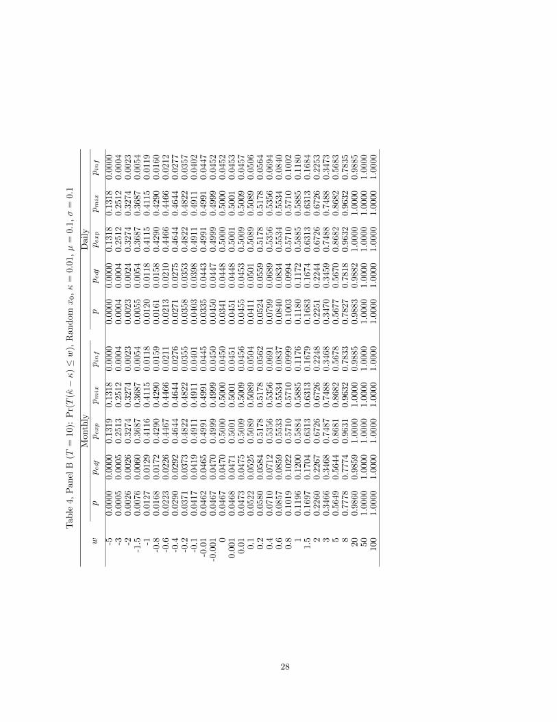
Tab
le4,
Pan
elB
(T=
10):
Pr(T
(κ−κ
)≤w
),R
an
domx0,κ
=0.
01,µ
=0.
1,σ
=0.
1
Month
lyD
ail
yw
ppedf
pexp
pmix
pinf
ppedf
pexp
pmix
pinf
-50.
0000
0.00
00
0.1
319
0.1
318
0.0
000
0.0
000
0.0
000
0.1
318
0.1
318
0.0
000
-30.
0005
0.00
05
0.2
513
0.2
512
0.0
004
0.0
004
0.0
004
0.2
512
0.2
512
0.0
004
-20.
0026
0.00
26
0.3
274
0.3
274
0.0
023
0.0
023
0.0
024
0.3
274
0.3
274
0.0
023
-1.5
0.00
760.
0060
0.3
687
0.3
687
0.0
054
0.0
055
0.0
054
0.3
687
0.3687
0.0
054
-10.
0127
0.01
29
0.4
116
0.4
115
0.0
118
0.0
120
0.0
118
0.4
115
0.4
115
0.0
119
-0.8
0.01
680.
0172
0.4
290
0.4
290
0.0
159
0.0
161
0.0
158
0.4
290
0.4290
0.0
160
-0.6
0.02
230.
0226
0.4
467
0.4
466
0.0
211
0.0
213
0.0
210
0.4
466
0.4466
0.0
212
-0.4
0.02
900.
0292
0.4
644
0.4
644
0.0
276
0.0
271
0.0
275
0.4
644
0.4644
0.0
277
-0.2
0.03
710.
0373
0.4
822
0.4
822
0.0
355
0.0
358
0.0
353
0.4
822
0.4822
0.0
357
-0.1
0.04
170.
0419
0.4
911
0.4
911
0.0
401
0.0
403
0.0
398
0.4
911
0.4911
0.0
402
-0.0
10.
0462
0.04
65
0.4
991
0.4
991
0.0
445
0.0
335
0.0
443
0.4
991
0.4
991
0.0
447
-0.0
010.
0467
0.04
70
0.4
999
0.4
999
0.0
450
0.0
450
0.0
447
0.4
999
0.4999
0.0
452
00.
0467
0.04
70
0.5
000
0.5
000
0.0
450
0.0
341
0.0
448
0.5
000
0.5
000
0.0
452
0.00
10.
0468
0.04
71
0.5
001
0.5
001
0.0
451
0.0
451
0.0
448
0.5
001
0.5
001
0.0
453
0.01
0.04
730.
0475
0.5
009
0.5
009
0.0
456
0.0
455
0.0
453
0.5
009
0.5009
0.0
457
0.1
0.05
220.
0525
0.5
089
0.5
089
0.0
504
0.0
411
0.0
501
0.5
089
0.5
089
0.0
506
0.2
0.05
800.
0584
0.5
178
0.5
178
0.0
562
0.0
524
0.0
559
0.5
178
0.5
178
0.0
564
0.4
0.07
100.
0712
0.5
356
0.5
356
0.0
691
0.0
799
0.0
689
0.5
356
0.5
356
0.0
694
0.6
0.08
570.
0859
0.5
533
0.5
534
0.0
837
0.0
840
0.0
834
0.5
534
0.5
534
0.0
840
0.8
0.10
190.
1022
0.5
710
0.5
710
0.0
999
0.1
003
0.0
994
0.5
710
0.5
710
0.1
002
10.
1196
0.12
00
0.5
884
0.5
885
0.1
176
0.1
180
0.1
172
0.5
885
0.5885
0.1
180
1.5
0.16
970.
1704
0.6
313
0.6
313
0.1
679
0.1
683
0.1
674
0.6
313
0.6
313
0.1
684
20.
2260
0.22
67
0.6
726
0.6
726
0.2
248
0.2
251
0.2
244
0.6
726
0.6726
0.2
253
30.
3466
0.34
68
0.7
487
0.7
488
0.3
468
0.3
470
0.3
459
0.7
488
0.7488
0.3
473
50.
5649
0.56
44
0.8
681
0.8
682
0.5
678
0.5
677
0.5
670
0.8
682
0.8682
0.5
683
80.
7778
0.77
74
0.9
631
0.9
632
0.7
833
0.7
827
0.7
818
0.9
632
0.9632
0.7
835
200.
9860
0.98
59
1.0
000
1.0
000
0.9
885
0.9
883
0.9
882
1.0
000
1.0
000
0.9
885
501.
0000
1.00
00
1.0
000
1.0
000
1.0
000
1.0
000
1.0
000
1.0
000
1.0
000
1.0
000
100
1.00
001.
0000
1.0
000
1.0
000
1.0
000
1.0
000
1.0
000
1.0
000
1.0000
1.0
000
28

References
Aıt-Sahalia, Y., 2002, Maximum likelihood estimation of discretely sampled diffusion: A closed-form approxi-mation approach. Econometrica 70, 223–262.
Ali, M.M., 2002, Distribution of the least squares estimator in a first-order autoregressive model. EconometricReviews 21, 89–119.
Ansley, C.F., R. Kohn, and T.S. Shively, 1992, Computing p-values for the Generalized Durbin-Watson andother invariant test statistics. Journal of Econometrics 54, 277–300.
Bandi, F.M. and P.C.B. Phillips, 2003, Fully nonparametric estimation of scalar diffusion models. Econometrica71, 241–283.
Bandi, F.M. and P.C.B. Phillips, 2007, A simple approach to the parametric estimation of potentially nonsta-tionary diffusions. Journal of Econometrics 137, 354–395.
Bernstein, D.S., 2009, Matrix Mathematics: Theory, Facts, and Formulas (Second Edition). Princeton Uni-versity Press, New Jersey.
Bierens, H., 2000, Nonparametric nonlinear co-trending analysis, with an application to inflation and interestin the U.S. Journal of Business & Economic Statistics 18, 323–337.
Black, F. and M. Scholes, 1973, The pricing of options and corporate liabilities. Journal of Political Economy81, 637–654.
Brown, B.W. and J.T. Hewitt, 1975, Asymptotic likelihood theory for diffusion processes. Journal of AppliedProbability 12, 228–238.
Davies, R.B., 1973, Numerical inversion of a characteristic function. Biometrika 60, 416.
Davies, R.B., 1980, Algorithm AS 155: The distribution of a linear combination of χ2 random variables. TheAmerican Statistician 29, 323–333.
Elliott, G. and U.K. Muller, 2006, Minimizing the impact of the initial condition on testing for unit roots.Journal of Econometrics 135, 285–310.
Fulop, A., J. Li, and J. Yu, 2011, Bayesian learning of impacts of self-exciting jumps in returns and volatility.Working paper, Singapore Management University.
Gil-Pelaez, J., 1951, Note on the inversion theorem. Biometrika 38, 481–482.
Gurland, J., 1948, Inversion formula for the distribution of ratios. Annals of Mathematical Statistics 19,228–237.
Hillier, G., 2001, The density of a quadratic form in a vector uniformly distributed on the n-sphere. EconometricTheory 17, 1–28.
Hong, Y., and H. Li, 2005, Nonparametric specification testing for continuous time model with application tospot interest rates. Review of Financial Studies 18, 37–84.
Hurwicz, L., 1950, Least squares bias in time series, in: T.C. Koopmans (Ed.), Statistical Inference in DynamicModels, Wiley, New York, pp. 365–383.
Imhof, J.P., 1961, Computing the distribution of quadratic forms in normal variables. Biometrika 48, 419–426.
Lu, Z.-H. and M.L. King, 2002, Improving the numerical technique for computing the accumulated distributionof a quadratic form in normal variables. Econometric Reviews 21, 149–165.
29

Merton, R.C., 1971, Optimum consumption and portfolio rules in a continuous time model. Journal of Eco-nomic Theory 3, 373–413.
Muller, U.K. and G. Elliott, 2003, Tests for unit roots and the initial condition. Econometrica 71, 1269–1286.
Perron, P., 1989, The calculation of the limiting distribution of the least-squares estimator in a near-integratedmodel. Econometric Theory 5, 241–255.
Phillips, P.C.B. and J. Yu, 2005, Jackknifing bond option prices. Review of Financial Studies 18, 707–742.
Phillips, P.C.B. and J. Yu, 2009a, Simulation-based estimation of contingent-claims prices. Review of FinancialStudies 22, 3669–3705.
Phillips, P.C.B. and J. Yu, 2009b, A two-stage realized volatility approach to estimation of diffusion processeswith discrete data. Journal of Econometrics, 150, 139–150.
Phillips, P.C.B. and J. Yu, 2009c, Maximum likelihood and Gaussian estimation of continuous time models infinance, in: T. G. Andersen, R.A. Davis, J.-P. Kreiß, and T. Mikosch (Eds.), Handbook of Financial TimeSeries, Springer-Verlag, New York, pp. 497–530.
Singleton, K., 2001, Estimation of affine pricing models using the empirical characteristic function. Journal ofEconometrics 102, 111–141.
Sundaresan, S.M., 2000, Continuous-time methods in finance: A review and an assessment. Journal of Finance55, 1569–1622.
Tang, C.Y. and S.X. Chen, 2009, Parameter estimation and bias correction for diffusion processes. Journal ofEconometrics, 149, 65–81.
Tsui, A.K. and M.M. Ali, 1992, Approximations to the distribution of the least squares estimator in a first-orderstationary autoregressive model. Communications in Statistics-Simulation 21, 463–484.
Tsui, A.K. and M.M. Ali, 1994, Exact distributions, density functions and moments of the least squaresestimator in a first-order autoregressive model. Computational Statistics and Data Analysis 17, 433–454.
Ullah, A., 2004, Finite Sample Econometrics. Oxford University Press, New York.
Vasicek, O., 1977, An equilibrium characterization of the term structure. Journal of Financial Economics 5,177–188.
Yu, J., 2012, Bias in the estimation of the mean reversion parameter in continuous time models. Journal ofEconometrics 169, 114–122.
Zhang, L., P.A. Mykland, and Y. Aıt-Sahalia, 2011, Edgeworth expansions for realized volatility and relatedestimators. Journal of Econometrics 160, 190–203.
Zhou, Q. and J. Yu, 2010, Asymptotic distributions of the least square estimator for diffusion processes.Working Paper, Singapore Management University.
30