Exact Energy Bands and Fermi Surfaces of

Separable Abelian Potentials

E D Belokolos,∗ J C Eilbeck,† V.Z. Enolskii,‡ and M Salerno §

Abstract

We present a general theory for multidimensional Schrodinger equations with

separable Abelian potentials with an arbitrary number of gaps in the spec-

trum. In particular we derive general equations which allow to express the

energy and the wave vectors in the BZ as a function of the spectral param-

eters. By using the solutions of these equations, we show how to construct

the energy bands and the Fermi surfaces in the first Brillouin zone of the

reciprocal lattice. As illustrative examples we consider the case of 2D sepa-

rable potentials with 1-, 2-, and 3-gaps in the spectrum. The method can be

applied to crystals with a cubic or a rectangular parallelogram Wigner-Seitz

cell in arbitrary dimensions. The possibility to generalize the theory to other

crystal symmetries is also briefly discussed.

∗Department of Theoretical Physics, NASU Institute of Magnetism 36-b Vernadsky str., Kiev-680,

03142,Ukraine. email: bel@imag.kiev.ua

†Department of Mathematics, Heriot-Watt University, Riccarton, Edinburgh EH14 4AS, UK.

email:J.C.Eilbeck@hw.ac.uk

‡Department of Theoretical Physics, NASU Institute of Magnetism 36-b Vernadsky str., Kiev-680,

03142,Ukraine. email: vze@imag.kiev.ua

§Dipartimento di Scienze Fisiche “E.R.Caianiello” and INFM Unita’ di Salerno, via S. Allende,

I-84081, Baronissi (SA), Italy. email: salerno@sa.infn.it

1

PACS: 02.10.Rn, 02.30.Jr, 71.18+y, 71.20-b

2

I. INTRODUCTION

The general theory of the many-dimensional Schrodinger operator was

established many years ago, i.e. immediately after the advent of quantum

mechanics. Since the pioneering work of F. Bloch [1], in which the spectral

properties of these operators were first recognised to be of fundamental im-

portance for the quantum theory of solids, much work has been done. This

lead to the development of the band theory, one of the pillars of modern Solid

State Physics. In spite of this, only a few examples are known of Schrodinger

operators with periodic potentials, allowing exact analytical calculations of

energy bands and Fermi surfaces.

Although numerical and self-consistent methods to compute the band

structure of a solid with good accuracy exist, it is desirable to have exact

solutions of the Schrodinger equation. These solutions, for some physically

relevant multidimensional periodic potentials, are useful not only for compar-

ison with approximate approaches, but also for further developments of the

general theory. This would allow, for example, to get a deep understanding

of the spectral manifolds and of the corresponding eigenfunctions, as well as

of their geometrical and analytical properties.

From a mathematical point of view, the most interesting periodic po-

tentials are the ones which can be expressed in terms of Abelian functions

(Abelian potentials). Abelian functions are multiply periodic functions be-

ing defined on complex tori, which can be considered in the context of the

problem as a siutable complexification of the real crystal lattice and its dual.

In some sense they are the analogues of the potentials in classical mechanics

which allow a complexification of the Liouville tori leading to Jacobians and

Abelian functions and hence to algebraic integrable systems. It is remarkable

that although the theory of such potentials was developed long before the ad-

3

vent of quantum mechanics, they have been almost ignored by the Solid State

Physics community. On the contrary, we think these potentials are important

and should be considered in Solid State Physics as being the equivalent of Ke-

pler’s problem for atomic physics. They give the opportunity to study many

questions related to the electronic properties of solids in a clear geometrical

and analytical form.

In this paper we are interested in multidimensional separable general-

izations of the simplest possible Abelian potential, i.e. the one expressed as

Weierstrass elliptic function ℘(z), with one real and one pure imaginary pe-

riod. The Schrodinger operator with such a potential has exactly 1-gap spec-

trum and allows to obtain eigenfunctions in an explicit form (in the math-

ematical literature this equation is known as the 1D Lame equation). This

spectral problem is essentially easier and more clear than e.g. the well known

Kronig-Penney problem, and can be used as a building block of a multidimen-

sional theory. Our extensions to this problem are twofold: one is to consider

multi-gap spectrum (a well studied problem), and the second to extend these

multi-gap results to higher dimensions.

The investigation of the 1D Lame equation was very well developed in the

classical monographs of Halphen [2], Krause [3], Forsyth [4], and Whittaker

and Watson [5]. Arscott [6,7] has surveyed results on the Jacobian form of the

Lame equation. The Lame equation has also figured prominently in a number

of recent publications devoted to study of completely integrable systems of

KdV type: Krichever [8], Eilbeck and Enol’skii [9], Enol’skii and Kostov [10],

Smirnov [11], Gesztesy and Weikard [12,13], Zabrodin [14], and others.

The aim of the present paper is to present the general theory for multi-

dimensional Schrodinger equations with separable Abelian potentials with an

arbitrary number of gaps in the spectrum (by separable here we mean those

potentials which can be written as a sum of N 1-dimensional finite-gap poten-

4

tial, one for each spatial dimension). The introduction of separable Abelian

potentials and their application to problems of solid state physics was also

considered in [15,16] for potentials with one and two gaps in the spectrum.

Our results allow us to express the energy and the wave vectors in the Bril-

louin Zone (BZ) as a function of the spectral parameters. The edges of the

bands also follow from these equations as roots of specific polynomials. From a

mathematical point of view this corresponds to the problem of constructing a

hyperelliptic N -sheeted covering, N = g(g +1)/2 over a torus (elliptic curve),

first considered by Jacobi and developed further by Weierstrass, Poincare and

others, see [17] and [18] for a detailed exposition.

By using the solutions of these equations for the spectral parameters, we

show how to construct the energy bands and the Fermi surfaces in the first

Brillouin zone of the reciprocal lattice. As illustrative examples we consider

the case of 2D separable potentials with a 1-, 2-, and 3-gap spectrum. The

method, although not restricted to 2D, can be applied only to crystals with

a cubic or a rectangular parallelogram Wigner-Seitz cell. Possible physical

applications of our theory, as well as its generalization to other crystal sym-

metries will be briefly discussed at the end of the paper.

The paper is organised as follow. In Section 2 we present the mathe-

matical theory of separable N-dimensional Abelian potentials and the general

equations valid in the case of arbitrary gaps in the spectrum. In Section 3 we

present detailed calculations of bands and Fermi curves for 2D lattices with

both square and rectangular symmetry. In the Conclusion we discuss possible

physical applications of these results to different problems.

II. SEPARABLE ABELIAN G-GAP PERIODIC POTENTIALS

The N -dimensional Schrodinger operator with the separable potential

5

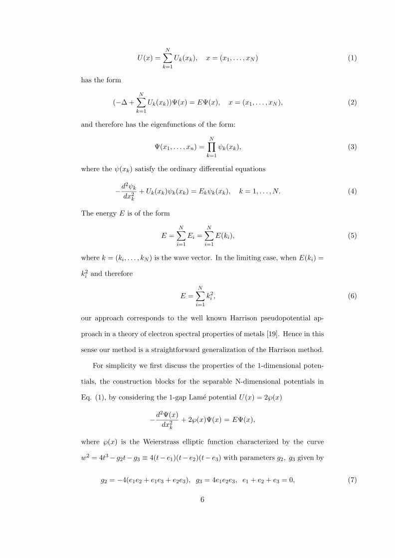
U(x) =N∑

k=1

Uk(xk), x = (x1, . . . , xN ) (1)

has the form

(−∆ +N∑

k=1

Uk(xk))Ψ(x) = EΨ(x), x = (x1, . . . , xN ), (2)

and therefore has the eigenfunctions of the form:

Ψ(x1, . . . , xn) =N∏

k=1

ψk(xk), (3)

where the ψ(xk) satisfy the ordinary differential equations

−d2ψk

dx2k

+ Uk(xk)ψk(xk) = Ekψk(xk), k = 1, . . . , N. (4)

The energy E is of the form

E =N∑

i=1

Ei =N∑

i=1

E(ki), (5)

where k = (ki, . . . , kN ) is the wave vector. In the limiting case, when E(ki) =

k2i and therefore

E =N∑

i=1

k2i , (6)

our approach corresponds to the well known Harrison pseudopotential ap-

proach in a theory of electron spectral properties of metals [19]. Hence in this

sense our method is a straightforward generalization of the Harrison method.

For simplicity we first discuss the properties of the 1-dimensional poten-

tials, the construction blocks for the separable N-dimensional potentials in

Eq. (1), by considering the 1-gap Lame potential U(x) = 2℘(x)

−d2Ψ(x)dx2

k

+ 2℘(x)Ψ(x) = EΨ(x),

where ℘(x) is the Weierstrass elliptic function characterized by the curve

w2 = 4t3− g2t− g3 ≡ 4(t− e1)(t− e2)(t− e3) with parameters g2, g3 given by

g2 = −4(e1e2 + e1e3 + e2e3), g3 = 4e1e2e3, e1 + e2 + e3 = 0, (7)

6

(below we will show how these parameters are related to the boundaries of the

spectra). It is known that the eigenfunction and the corresponding eigenvalues

of this equation can be expressed as [5]

Ψ(x; a) =σ(a− x)σ(x)σ(a)

exp{xζ(a)}, E = ℘(a), (8)

where a denotes a spectral parameter and σ the Weierstrass σ-function related

to the Weierestrass ℘ and ζ functions by the relations

ζ(u) =∂

∂ulnσ(u), ℘(u) = − ∂2

∂u2lnσ(u) = − ∂

∂uζ(u).

The above wave functions can be rewritten in the form of a Bloch function as

Ψ(ix; a) = eik(a)xB(ix; a), B(ix; a) =σ(a− ix)σ(ix)σ(a)

exp{i η′

ω′ax} (9)

where we take x → ix and introduced the wave vector k(a) as

k(a) = ζ(a)− η′

ω′a (10)

Note that x imaginary does not effect the reality of the potential and it

implies that the periodicity of the potential is Im(2ω′) where 2ω

′denotes the

imaginary period of the ℘ function. The ratio η′/ω′ is real since η′ , the second

imaginary period, is purely imaginary. One can then easily prove that (9) is

nothing but the Floquet theorem [20] for the 1-gap Lame potential. Indeed,

by using the periodicity property of the σ function

σ(u + 2mω + 2m′ω′) = (−1)mm′+m+m′σ(u)e(u+mω+m′ω′)(2ηm+2η′m′) (11)

and denoting the translation operator by one period of the potential by

TIm(2ω′), we have that

TIm(2ω′)Ψ(ix; a) = Ψ(ix + 2ω

′; a) = eik(a)Im(2ω

′) Ψ(ix; a) (12)

from which we see that Ψ is an eigenfunction of the translation operator

associated with the eigenvalue eik(a)Im(2ω′) (this implies that B(ix; a) is a

7

periodic function with period Im(2ω′)). Note that for the multidimensional

separable wavefunction (3), eq. (12) automatically leads to the usual Bloch

theorem [1]. An equation for the spectral parameter a can be obtained by

observing that the function

Λ(u) = ℘(u)− ℘(a) (13)

is a solution of the equation

d3Λd3u

− 4(2℘(u) + E)dΛdu

− 4℘′(u)Λ = 0. (14)

Inserting (13) into (14) gives the expression for the energy E in terms of the

quantity a

E = ℘(a). (15)

In this case we simply obtain the relation between the energy and the spectral

parameter. However, in the general g-gap case, we will get a set of g equa-

tions among the spectral parameters. For the g = 1 case, Eq. (15) uniquely

determines the energy bands. The reality condition of the energy and the

properties of the ℘ function imply that the spectrum must lie in the intervals

[e3, e2] and [e1,∞] (see below). Note that the equations (10) and (15) express

the energy E in terms of the wave vector k in parametric form.

These expressions can be easily generalized to the case of the one dimen-

sional Schrodinger equation with g-gap Lame potentials U(x) = g(g + 1)℘(x)

−d2Ψ(xk)dx2

k

+ g(g + 1)℘(xk)Ψ(xk) = E Ψ(xk).

One can check that the eigenfunctions can be written as

Ψ(x, a1, ..., ag) = eik(a1,...,ag)xg∏

j=1

σ(aj − ix)σ(ix)σ(aj)

exp{ixg∑

j=1

η′

ω′aj}. (16)

with the wavevector k given by the expression

8

k(a1, ..., ag) =g∑

j=1

[ζ(aj)− η′

ω′aj ]. (17)

The equations for the spectral parameters aj , j = 1, . . . , g can be determined

from the fact that

Λ(u) =g∏

j=1

[℘(u)− ℘(aj)] (18)

is a solution of the equation

d3Λd3u

− 4(g(g + 1)℘(u) + E)dΛdu

− 2g(g + 1)℘′(u)Λ = 0. (19)

Inserting (18) into (19) gives the following system of algebraic equations for

the quantities ℘(aj)

αkESk−1 + βk g2Sk−2 + γkg3Sk−3 − δkSk = 0, k = 1, 2, ..., g, (20)

where Sk denotes the k-th elementary symmetric function

Sk =g∑

j1<j2<...<jk

℘(aj1)℘(aj2), ...℘(ajk), (21)

and

αk = 4(−1)k−1(k − g − 1),

βk =12(−1)k−1

(2(g − (k − 4))3 − 15(g − (k − 4))2 + 37(g − k + 4)− 30

),

γk = (−1)k(g − k + 3)(g − k + 2)(g − k + 1),

δk = 2k(−1)k(4g2 + 2g(2− 3k) + 2k2 − 3k + 1

).

(Note that in Eq. 20 we assume that S−k = 0 and S0 = 1). One can easily

check that the first equation (i.e. k = 1) of the system in (20) gives the energy

E in terms of the quantities aj , j = 1, . . . , g

E = (2g − 1)g∑

j=1

℘(aj), (22)

while the second and third equations (k=2,3) express the invariants g2, g3, in

terms of the energy and the quantities aj , j = 1, . . . , g,

9

g2 =8g

g∑j=1

℘2(aj) +S2

g − 1

, (23)

g3 =8g

2g − 32g

g∑i=1

℘3(ai)− 1g − 1

g∑i<j

(℘2(ai)℘(aj) + ℘(ai)℘2(aj)

)− 3(2g − 3)

(g − 1)(g − 2)S3

The other g − 3 equations establish additional relations between the aj . To

construct the energy bands as function of k one must solve the above system

of algebraic equations for the ℘(aj)′s together with a condition for the reality

of the energy. In the procedure one must invert the ℘ function to get the aj,

and use equations to relate the energy E to the wave vectors k in a paramet-

ric form. Although this looks complicated it can be easily performed on a

computer using one of the many parametric plot packages available.

Before presenting explicit numerical results let us discuss how to derive

from Eq. (20) the expression for the edges of the bands. We wish to write these

bands as a function of the parameters e1,e2, e3 characterising the underlying

elliptic curve. In order to do this one must add to the above general formulas

an extra condition which guarantee the reality of the energy (note that since

the energy is unknown, we actually have g equations for g + 1 unknowns).

This can be done by fixing one of the spectral parameters ai, say a1, so that

℘(a1) = ei. One can easily show that this choice will guarantee the reality

of the energy. By constructing the Groebner basis for the polynomial in Eqs

(20) one can eliminate the g − 1 variables ℘(ai), i = 2, ..., g, in favour of the

energy. This will lead to factorized polynomials which for g = 1, 2, 3, are given

respectively by

43∏

i=1

(E − ei), (24)

(E2 − 3g2

) 3∏i=1

(E + 3ei), (25)

E3∏

i=1

(E2 − 6eiE + 45e2i − 15g2). (26)

10

It is possible to set up a general procedure to determine these polynomials

(and therefore the edges of the bands) for potentials with an arbitrary number

of gaps. Thus, for example, for g = 5, 7, 9 we obtain

(E2 − 27g2)3∏

i=1

[E3 − 15eiE2 + (315e2

i − 132g2)E + 540g3 + 675e3i ],

(E3 − 196g2E + 2288g3)3∏

i=1

[E4 − 28eiE3 + (1134e2

i − 574g2)E2 +

(34100 ei

3 − 5116 eig2

)E + 59150 ei

2g2 − 528983 ei4 + 22113 g2

2 + 88452 g3ei]

(E4 − 774g2E2 + 21600g3E + 41769g2

2)3∏

i=1

[E5 − 45eiE4 + (2970e2

i − 1764g2)E3 +

(25380eig2 − 202230e3i )E

2 − (9461259e4i − 402624g2

2 − 1610496g3ei − 1210356e2i g2)E

−20241900e3i g2 + 37013760e2

i g3 − 76485465e5i + 9253440eig

22]

Notice that the problem of constructing these polynomials is related to the

problem of constructing coverings for hyperelliptic curves on a g-sheetedly

torus considered by Jacobi, Weierstrass and Poincare. For Lame potentials

with an arbitrary number of gaps, a solution of this problem can be obtained

from the above equations as will be discussed in a separate paper. Note that

the system of Eqs. in (20) refers to the g-gap 1D potential i.e. to the building

blocks of the higher dimensional cases. In the higher dimensional separable

case one must, of course, consider several of such systems, with different

spectral parameters and different elliptic curves, one for each dimension. In

the case in which the curves coincide, the systems of equations and their

corresponding solutions will obviously coincide. These will be discussed in

the next section.

11

III. ENERGY BANDS AND FERMI CURVES FOR 2D SEPARABLE

POTENTIALS

From a physical point of view, one is interested in computing the shapes

of the energy bands and the corresponding Fermi surfaces as a function of

the wave numbers in the first BZ. From this knowledge, important physical

properties of the system will follow, such as the density of states, the electron

effective mass, transport properties, etc. In this section we will show how this

can be done exactly for 2D separable elliptic potentials with one, two and

three gaps in the spectrum, using the theory described above (for simplicity

we restrict ourselves to the 2D case, but the construction is quite general

and can be applied to 3D as well). This will cover the cases of crystals with

a square or rectangular Wigner-Seitz cell and with 2, 3, 4 energy bands,

respectively.

More specifically, let us consider the potential

U(x, y) = g(g + 1)(℘(ix + ω) + ℘(iy + ω)) (27)

associated with two elliptic curves w2 = 4t3− g2t− g3 and w2 = 4t3− g2t− g3

(one for each spatial direction) with g2, g3 (and similarly for g2, g3 and ei, i =

1, 2, 3) related to the gap edges ei, i = 1, 2, 3 by Eqs. (7). Note that in

order to have a real and nonsingular potential for all x, y ∈ R, we have

taken the argument of the ℘ functions appearing in the potential, along the

imaginary axis shifted by the half real periods ω, ω of the corresponding elliptic

curve (recall that the ℘ function is singular at the origin). This implies that

the periodicity in the x and y directions are just the two imaginary periods

2ω′, 2ω

′.

We shall first consider the case of identical elliptic curves, this correspond-

ing to lattices with square Wigner-Seitz cells (the periodicity of the potential

12

in the x and y direction being the same). The case of different curves, associ-

ated with rectangular Wigner-Seitz cells, will be discussed at the end of this

section. In the following calculation we fix the parameters e1 = 2, e2 = −0.5,

e3 = −1.5 (and ei = ei), this correspondes to having fixed the real and the

imaginary periods

ω =∫ e2

e3

dt√4t3 − g2t− g3

, ω′=

∫ e1

e2

dt√4t3 − g2t− g3

,

η =∫ e2

e3

tdt√4t3 − g2t− g3

, η′=

∫ e1

e2

tdt√4t3 − g2t− g3

,

as 2ω = 1.82339, 2ω′ = 2.24176i, 2η = 1.7851, 2η′ = −1.25119i (note that

Legendre’s relation [5]: ηω′ − η′ω = iπ2 is satisfied).

In real applications, since the ei’s determine the edges of the energy bands,

one should consider them as parameters to be fixed by experiments. Let us

start with the one gap potential (g = 1 in Eq. (27)) which, being simple, will

be used to fix the notation and to check results. This potential is plotted

in Fig. 1 as a function of x, y, from which we see that it is periodic (with

the same period in both directions given by 2|ω′|), real and well behaved

over all space. In Fig. 2 the level curves of such potentials are reported

in the Wigner-Seitz cell. From Eqs. (20) we have for this case only one

equation (g = k = 1) which express the energy as a function of the “spectral”

parameters: E = ℘(a1)+℘(a1). Since the energy is additive in the ℘(ai), the

spectral parameters must vary on curves of the fundamental domain on which

℘ is real. These curves coincide with the intervals [0, 2ω] and [ω′, 2ω + ω′] in

correspondence of which the wavevectors kx = ζ(a1)− η′ω′a1, ky = ζ(a1)− η′

ω′

a1 will span the BZ [− π2|ω′| ,

π2|ω′| ]× [− π

2|ω′| ,π

2|ω′| ].

The energy bands in k-space are then obtained by parametrically plotting

E, kx, ky as functions of a1, a1 in the above intervals. This is shown in Fig. 3,

from which we see that the ranges of the lower and upper bands respectively

are [−3,−1] and [4,∞]. In terms of the spectral parameters this corresponds

13

to taking a1, a1 ∈ [ω′, 2ω + ω′], for the lower band, and a1, a1 ∈ [0, 2ω] for the

upper one. This is evident from the fact that ℘(ω′) = e3 = −1.5, ℘(ω +ω′) =

e2 = −0.5 and ℘(ω) = e1 = 2 (the bands edges are simply twice these values).

Also note that for bands symmetric in k (as in our case) one can restrict

to only half of these parameter intervals (the other half just reproduce the

symmetry). Since for a given band the energy is a continuous function of

kx, ky, one can draw curves of constant energy analogous to the equipotential

surfaces of electrostatics. One of these curves will be the so called Fermi

curve, i.e. the curve for which all states described by k-vectors within it will

be occupied and all k-vectors outside it will label unoccupied states. One can

easily show that this curve (in the 3D case a surface) has the symmetry of

the crystal, i.e. it is invariant under the point group operations characterizing

the lattice.

In Fig. 4 we plot the Fermi curves, i.e. the curves of constant energy,

as a function of kx, ky for different values of E. Note that at the bottom

and at the top of the bands, the Fermi curve are circles, as for the free

electron case, whilst for intermediate values they deform and perpendicularly

intersect the BZ boundaries. This fact is an indirect check on the correctness

of our calculations since from the general theory it is known that the Fermi

curve is always tangential to ∇E(k) and, for any reciprocal lattice vector K

perpendicularly joining opposite parallel faces of the BZ, one must have that

K · ∇E(k) = 0. In Fig. 5 the Bloch wave function at the bottom of the lower

band (ground state) is shown. It is an extended function both in x and y and

has maxima located in correspondence with the potential minima.

Let us now consider the case of two gaps in the spectrum (g = 2 in

Eq. (27)). From the system (20) we have two equations, one for the energy

and another for g2 as a function of the spectral parameters a1, a2. These

equations can be easily solved by taking a1 (similarly for a1) varying on the

14

same intervals as for the g = 1 case (this is a requirement for the reality

of the energy), and then solving the resulting quadratic equation for ℘(a2)

involving g2. By inverting the Weierstrass ℘ function we get a1, a2, which

can then be used to plot the energy as a function of the wavenumbers. In

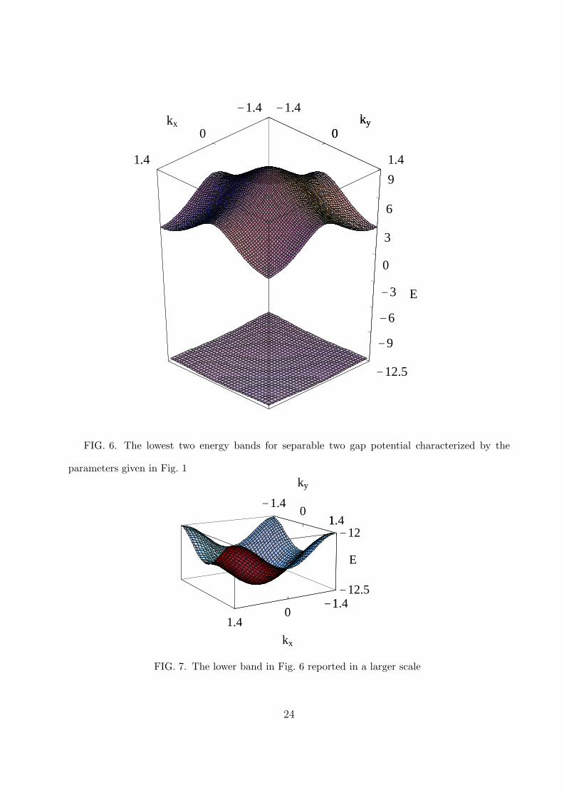
Fig. 6 the two lower bands for the 2D two gap potential are plotted for the

same parameters as before. In Fig. 7 we have shown the lowest band in higher

detail (the highest energy band is similar to the one of g = 1 and was omitted

for graphical convenience). In Figs. 8, 9, a set of Fermi curves for the two

lowest bands are also shown. From these figures we see for the lowest band the

same qualitative behavior as for the g = 1 case, but for the second band the

Fermi curves are now asymmetrical with respect to the center of the Brioullin

zone. In Fig. 10 the energy is plotted as a function of the spectral parameter

along the lines ai = ai, from which we see that the edges of the bands are in

agreement with the formula in Eq. (25) (in our case g2 = 13).

A similar analysis can be done for the 3 gap case. Now besides the energy

and the equation for g2 we have also the equation for g3. To find the spectral

parameters a1, a2, a3 in this case, one must numerically solve a quadratic and

a sextic equation. Since the energy bands look qualitatively similar to the

ones depicted in the previous cases, in Fig. 11 we show only the second lowest

band and in Fig. 12 the corresponding Fermi curves. Note that the small

gaps between the Fermi curves and the boundaries of the Brillouin zone are

due to numerical effects (we stopped before intersecting the boundary since

one needs higher precision i.e. longer computer time, to calculate the solution

in these regions. It is evident, however, that the intersection of the Fermi

curve with the edges of the Brillouin zone are always orthogonal. In Fig. 13

the energy bands are shown as functions of the spectral parameters. It is

interesting to note that the shape of the bands are different from the ones in

the reciprocal space (the second lowest band, for example, has a maximum in

15

the center as a function of the spectral parameter, while it has a minimum as

a function of the wavenumbers). The edges of these bands are

E = 0, E = 3ei ±√

9e2j + 15(ej − ek)2, (28)

plus cyclic permutations of i, j, k = 1, 2, 3, which are just the roots of the

polynomial in Eq. (26) (these values agree with the energy gaps derived by

Smirnov in his reduction studies of elliptic potentials [21]).

Before closing this section we wish to discuss the case of lattices with rect-

angular Wigner-Seitz cells. This corresponds to the general case of different

elliptic curves associated with each space direction. In Fig. 14 the level sets

of a potential of this type are plotted (small circles correspond to maxima

and large ones to minima). Here the periodicity in the x direction is charac-

terized by the same elliptic curve as before, but for the one in the y direction

we take the curve with parameters e1 = 4, e2 = −1, e3 = −3 and with real

and imaginary periods given by 2ω = 1.82339, 2ω′ = 2.24176i, 2η = 1.7851,

2η′ = −1.25119i. The Brillouin zone is then also rectangular with extensions

[− π2|ω′| ,

π2|ω′| ] × [− π

2|ω′| ,π

2|ω′| ]. In Fig. 15 the two bands of the g = 1 potential

on a tectangular lattice are reported as function of wavevectors in the first

BZ. In contrast with the square lattice case, both bands are asymmetric in

the two directions, with edges given by −4.5,−1.5, 6. These numbers are just

the sums of the edges of the two separate elliptic curves, e1 + e1, e2 + e2,

e3 + e3. Moreover, from Fig. 16 we see that, due to the asymmetry, the Fermi

curves intersect the Brioullin zone boundaries first in ky and then in the kx

direction.

It is interesting to note that, although the Fermi curve approaches the

boundary tangentially, after the intersection it always becomes orthogonal to

it. We also note that at the bottom and at the top the behavior is very similar

as for the square lattices, i.e. the curves are circles as for free electrons. From

16

this analysis one can easily get a qualitative picture of the behavior of the

bands and of the Fermi curves for the multigap 2D potentials on rectangular

lattices, and therefore we will not discuss them further here. In closing this

paper we wish to remark that with semiconductor nano-technologies, it is

possible today to construct artificial solids in 2D dimensions as arrays of

quantum dots [22]. With electrode deposition techniques [23], it could indeed

be possible to construct periodic gates on top of a quantum well so as to

create smooth 2D potentials of the type described in this paper. Moreover,

the generalization of our analysis to 3D potentials, with a Wigner Seitz cell

which is a cube or a rectangular parallelogram, can easily be done.

We hope to generalize our results to lattices of some other spatial sym-

metry by means of the Trebich-Verdier and Smirnov potentials (see e.g. [24]).

But the extension of this method to lattices of general spatial symmetry with

separable multidimensional Lame potentials seems problematical. In this case,

however, potentials arising from hyperelliptic extensions of this theory, can

be useful. This generalization is presently under investigation [25].

Acknowledgments The research of the second and fourth authors was

supported in part by the INTAS grant 93-1324-Ext. The research of the third

author was supported in part by the CRDF grant and INTAS grants 93-1324-

Ext and INTAS-96-770. JCE and MS are also grateful for support under the

LOCNET EU network HPRN-CT-1999-00163.

17

REFERENCES

[1] F. Bloch. Quantum mechanics of electrons in crystal lattices. Zeits. f. Physik, 52:555–600,

1928.

[2] G. H. Halphen. Traite des Fonction Elliptiques, volume 2. Gauthier-Villars, Paris, 1888.

[3] M. Krause. Theorie der doppeltperiodischen Funktionen einer veranderlichen Grosse, volume 1.

Teubner, 1895.

[4] A. R. Forsyth. Theory of Differential Equations. Dover, 1959. Part III, Vol. 4.

[5] E. T. Whittaker and G. N. Watson. A Course of Modern Analysis. Cambridge University

Press, 1969.

[6] F. M. Arscott and I. M. Khabaza. Tables of Lame Polynomials, volume 17 of Mathematical

tables series. Pergamon, Oxford, 1962.

[7] F. M. Arscott. Periodic differential equations: an introduction to Mathieu, Lame, and allied

functions, volume 66 of International series of monographs in pure and applied mathematics.

Pergamon, Oxford, 1964.

[8] I. M. Krichever. Elliptic solutions of the Kadomtsev-Petviashvili equation and integrable sys-

tems of particles on a line. Funct. Anal. Appl., 14:282–290, 1980.

[9] J. C. Eilbeck and V. Z. Enol’skii. Elliptic Bake-Akhiezer functions and an application to an

integrable dynamical system. J. Math. Phys., 35:1192–1201, 1994.

[10] V. Z. Enol’skii and N. A. Kostov. On the geometry of elliptic solitons. Acta Appl.Math.,

36:57–58, 1994.

[11] A. O. Smirnov. Finite-gap elliptic solutions of the KdV equation. Acta Appl. Math., 36:125–

166, 1994.

[12] F. Gesztesy and R. Weikard. Lame potentials and the (m)KdV hierarchy. Math. Nachr.,

176:73–91, 1995.

18

[13] F. Gesztesy and R. Weikard. Elliptic algebro-geometric solutions of the KdV and AKNS

hierarchies - an analytic approach. Bull. AMS, 35:271–317, 1998.

[14] A. Zabrodin. On the spectral curve of the difference Lame operator. IMRN, 11:589–614, 1999.

[15] V. G. Bar’yakhtar, E. D. Belokolos, and A. M. Korostil. A new method for calculating the

electron spectrum in solids: application to high-temperature superconductors. Phys. Stat.

Sol.(b), 169:105–114, 1992.

[16] V. G. Bar’yakhtar, E. D. Belokolos, and A. M. Korostil. Method of separable finite-band

potential: a new method for calculating electron energy spectrum of solids. Phys. Metals,

12:829–838, 1993.

[17] A. Krazer. Lehrbuch der Thetafunctionen. Teubner, 1903. reprinted by Chelsea, 1998.

[18] E. D. Belokolos, A. I. Bobenko, V. Z. Enol’skii, A. R. Its, and V. B. Matveev. Algebro Geo-

metrical Aproach to Nonlinear Integrable Equations. Springer, Berlin, 1994.

[19] W. A. Harrison. Pseudopotentials in the Theory of Metals. Benjamin, New York, 1966.

[20] G. Floquet. Sur les equations differentielles lineaires a coefficients periodiques. Ann. Sci. Ecole

Norm., Super. (2), XII:47–89, 1883.

[21] A. O. Smirnov. On a class of elliptic potentials of the Dirac operator. Math USSR Sbornik,

188:115–135, 1997.

[22] L. Jacak, P. Hawrylak, and A. Wojs. Quantum Dots. Springer, 1998.

[23] J. P. Kotthaus J. Alsmeier, E. Batke. Voltage-tunable quantum dots on silicon. Phys. Rev. B,

41:1699–1702, 1990.

[24] V. G. Bar’yakhtar, E. D. Belokolos, and A. M. Korostil. Fermi-surfaces of metals with fcc

structures in the model of finite-band potential. Metalofizika, 15:3–13, 1993. (in Russian).

[25] V. M. Buchstaber, V. Z. Enol’skii, J. C. Eilbeck, D. V. Leykin, and M. Salerno. 2D Schrodinger

19

equations with Abelian potentials. In preparation, 2000.

20

FIGURES

-2.24

0

2.24

x

-2.24

0

2.24

y

-2

7.5

U

24

0x

FIG. 1. Potential profile in the one-gap case with parameters values e1 = 2, e2 = −0.5, e3 = −1.5

-1 -0.5 0 0.5 1

-1

-0.5

0

0.5

1

FIG. 2. Level curves of the potential in Fig. 1

21

-1.40

1.4

kx-1.4

01.4

ky

-3

-1

2

4

8

E

1.40

FIG. 3. Energy bands of the first Brillouin zone for the potential in Fig. 1. The edges of the

Brillouin zone (i.e. ± π2|ω′|) for the parameters chosen in Fig.1 correspond to the values ±1.401396

-1 0 1

-1

0

17.57.57.57.57.5

-1 0 1

-1

0

1-1.2-1.2-1.2-1.2-1.2

-1 0 1

-1

0

1-2.9-2.9-2.9-2.9-2.9

-1 0 1

-1

0

1-1.9-1.9-1.9-1.9-1.9

FIG. 4. Fermi curves relative to the energy bands of Fig. 3. The constant energy value at which

the curves are taken is reported at the right top of each figure

22

-2.24

0

2.24

x-2.24

0

2.24

y

00.20.40.60.8

4

0x

FIG. 5. Modulo squared of the wave function of the ground state for the potential in Fig. 1.

The energy is E = −3 corresponding to the bottom of the first band in Fig. 2.

23

-1.4

0

1.4

kx

-1.4

0

1.4

ky

-12.5

-9

-6

-3

0

3

6

9

E

0ky

FIG. 6. The lowest two energy bands for separable two gap potential characterized by the

parameters given in Fig. 1

-1.40

1.4

kx

-1.40

1.4

ky

-12

-12.5

E

-10

1.

FIG. 7. The lower band in Fig. 6 reported in a larger scale

24

-1.4 1.4kx

-1.4

1.4

ky

-12.1

-1.4 1.4kx

-1.4

1.4

ky

-12.22

-1.4 1.4kx

-1.4

1.4

ky

-12.48

-1.4 1.4kx

-1.4

1.4

ky

-12.25

FIG. 8. Fermi curves relative to the first (lower) band of Fig. 6. The top right of each figure

shows the constant energy value at which the curve is taken.

-1.4 1.4kx

-1.4

1.4

ky

8.95

-1.4 1.4kx

-1.4

1.4

ky

6.55

-1.4 1.4kx

-1.4

1.4

ky

3.35

-1.4 1.4kx

-1.4

1.4

ky

5.25

FIG. 9. Same as in Fig. 8 but for the second band of Fig. 6.

25

-0.75 -0.5 -0.25 0 0.25 0.5 0.75

-10

-5

0

5

10

15

20

FIG. 10. Energy curves as functions of the spectral parameters for α = β ∈ [−ω/2, ω′/2]. The

edges of the energy bands are −2√

3g2, −6e1, −6e2, −6e3, 2√

3g2, with e1, e2, e3 as in Fig. 1

kx

ky

-3

0

E

kx

ky

26

FIG. 11. Second lowest energy band for the 3-gap case. The parameters of the curves are fixed

as in Fig. 1

kx

ky

-0.15

kx

ky

-1.1

kx

ky

-2.1

kx

ky

-1.2

FIG. 12. Fermi curves relative to the band in Fig. 11.

0 0.25 0.5 0.75 1 1.25 1.5 1.75-30

-20

-10

0

10

20

30

FIG. 13. Energy curves as functions of the spectral parameters for α = β ∈ [0, 2ω] for the 3-gap

case. The edges of the energy bands are the root of the polynomial in Eq. (26).

27

-2 -1 0 1 2-1.5

-1

-0.5

0

0.5

1

1.5

FIG. 14. Level curves of 1-gap potential characterized by two different curves. The first curve

characterizing the x direction has the same parameters as in Fig. 1, whilst the other has parameter

e1 = 4, e2 = −1, e3 = −3.

28

-1.401.4

kx-1.9

01.9

ky

-4.5

-1.50

2

4

6

E

1.90

FIG. 15. Energy bands in the first Brillouin zone for the potential in Fig. 14.

29

-1 0 1

-101

-2.51-2.51-2.51-2.51-2.51

-1 0 1

-101

-1.6-1.6-1.6-1.6-1.6

-1 0 1

-1

0

1

6.36.36.36.36.3

-1 0 1

-101

-4.4-4.4-4.4-4.4-4.4

-1 0 1

-101

-3.5-3.5-3.5-3.5-3.5

-1 0 1

-1

0

1

-3-3-3-3-3

FIG. 16. Fermi curves in the first Brillouin zone for the bands in Fig. 15.

30