EXACT EQUILIBRIUM CRYSTAL SHAPES

IN TWO DIMENSIONS ; * '

AND

PERTURBATION EXPANSIONS FOR

THE FACET SHAPE AND STEP FREE ENERGY OF

A THREE-DIMENSIONAL EQUILIBRIUM CRYSTAL

Mark Holzer

B. Sc. (Honours), Simon Fraser University, 1984

A THESIS SUBMITIED IN PARTIAL FULFILLMENT OF

THE REQUIREMENTS FOR THE DEGREE OF

DOCTOR OF PHILOSOPHY

in the Department

of . "

Physics

O Mark Holzer 1990

SIMON FRASER UNIVERSITY

August, 1990

All rights reserved. This work may not be reproduced in whole or in part, by photocopy

or other means, without permission of the author.

APPROVAL

Name: * Y Markus Bernhard Holzer

Degree: Ph.D. Physics

Title of Thesis: Exact Equilibrium Crystal Shapes in Two Dimensions and Perturbation Expansions for the Facet Shape and Step Free Energy of a Three- Dimensional Equilibrium Crystal

Examining Committee:

Chairman: Prof. E. Daryl Crozier

- -. &T.'Gchael'~6ri~- '

Senior Supervisor

/ - \

Prof. Michael Plischke

Prof. Richard Enns

- - . - - 1 ma.-. - - Prof. Robert F. Frindt

Prof. Martin Grant

External Examiner Department of Physics

McGill University

Date Approved: 15 August. 1990

PARTIAL COPYRIGHT LICENSE

I hereby grant to Simon Fraser university the right

to lend my thesis, project or extended essay (the title of

which is shown gbiow) to users of the ~imon Fraser university

Library, and to make partial or single copies only for such

users or in response to a request from the library of any other

university, or other educational institution, on its own behalf

or for one of its users. I further agree that permission for

multiple copying of this work for scholarly purposes may be

granted by me or the Dean of Graduate Studies. It is

understood that copying or publication of this work for

financial gain shall not be allowed without my written

permission.

Title of Thesis/--

Exact Equilibrium Crystal Shapes in Two Dimensions and

perturbation Expansions For The Facet Shape and Step

Free Energy of a ~hree-~imensional ~quilibrium Crystal

Author: - (Signature)

Markus Bernhard HOLZER (Name)

. . . 111

Abstract P . * I

The fundamentals of the theory of equilibrium crystal shapes (ECS's) are

reviewed. The concepts developed are then applied to two model calculations:

Using a conceptually novel approach which maps a two-dimensional (2D) interface

exactly onto a Feynman-Vdovichenko lattice walker, we derive an exact and general

solution for the ECS of free-fermion models. The ECS for these models is given by the

locus of purely imaginary poles of the determinant of the "momentum-space" lattice-path

propagator. The ECS may, therefore, be read off simply from the analytical expression

for the bulk free energy. From these shapes one can then obtain numerically (but to

arbitrary accuracy) the anisotropic interfacial free energy per unit length and, therefore, the

high-temperature direction-dependent correlation length of the dual system. We give

several examples of previously unknowr, Ising ECS's, and we examine in detail the free-

fermion case of the eight-vertex model. The free-fermion eight-vertex model includes the

modified potassium dihydrogen phosphate (KDP) model, which is not in the Ising

universality class. The ECS of the modified KDP model is shown to be the limiting case

of the ECS of an antiferrornagfietic 2x1 phase on a triangular lattice in the limit of infinite

interactions. The ECS of the modified KDP model is lenticular at finite temperature and

has sharp comers. We explain the physics of this lens shape from an elementary

calculation.

To obtain the facet shapes and anisotropic step free energies for the 3D simple-

cubic nearest-neighbour Ising model, we develop systematic low-temperature perturbation

expansions about the exact solution for the ECS's and interfacial free energies of the 2D

square Ising model. An expansion scheme is developed which makes explicit use of the

conjugacy between the step free energy and the facet shape. We find that the facet shape is

approximated to better than 1% by the equilibrium crystal shape of the corresponding 2D g , '

Ising model for temperatures less than about 72% of the roughening temperature. In that

temperature range overhangs and bubbles contribute less than 0.1% to the step free

energy. At higher temperatures the facet shape is nearly circular with anisotropies of less

than 0.4% and a ratio of facet diameter to crystal diameter of less than 0.4. Extrapolations

into the isotropic region give critical roughening amplitudes consistent with recent Monte

Carlo data.

Acknowledgements

First andgofernost I thank my thesis advisor, Prof. M. Wortis, for many long

discussions, for innumerable helpful suggestions, for his clear pedagogical manner of

communicating physics which almost always turned my confusion into understanding, and

for his generosity and kindness. I consider myself very lucky to have an advisor who

always has time to discuss physics and who is unfailingly conscientious, encouraging, and

tolerant.

I am very grateful to M. Plischke for helpful discussions throughout my time as a

physics student, for his prompt, critical reading of my manuscripts, for his frank advice,

and for his positive influence in general.

On the subject of this thesis, I have enjoyed additional helpful discussions with M.

Rao and R. K. P. Zia.

Financial support from Simon Fraser University is gratefully acknowledged.

During my time as a graduate student, my understanding of physics has benefitted

substantially from discussions with many individuals. I am particularly thankful to S.

Breed, K. Heiderich, M. Hiirlimann, C. Lusher, A. H. MacDonald, and A. Roberge. . "

Especially inspiring and helpful were discussions with M. W. Reynolds.

I am also indebted to J. Berlinsky, P. Diamond, and M. N. Rosenbluth for

advising and directing me in my early studies of theoretical physics. I am grateful to W.

Hardy and R. Cline for tolerating me in their laboratory, where they generously provided

me with the opportunity to learn some of the skills of low-temperature experimental

physics.

Finally, I would like to thank my friends, and K. Heiderich in particular, for

providing moral support along with my parents.

Table of Contents

Approval 1 , ii ...

Abstract m

Acknowledgements v

Table of Contents vi ...

List of Tables w

List of Figures ix

Introduction 1

1 .1 The ECS as a classical variational problem and Wulff s Theorem 3

1.2 Formulations of Statistical Mechanics: Canonical and Grand Canonical Descriptions of the ECS 17

1.3 Organization and Motivation 24

A General, Exact Solution for Equilibrium Crystal Shapes in Two Dimensions for Free-Fermion Models 25

2.1 Introductory Remarks 25

2.2 Derivation 27

2.3 An example of non-Ising free-fennion crystal shapes: The modified KDP model 45

2.4 Conclusion 60

Low-Temperature Expansions For The Step Free Energy and Facet Shape of the Simple-Cubic Ising Model 62

3.1 Background and Introductory Remarks 62

3.2 Step free energies and facet shapes from interfacial free energies and equilibrium crystal shapes 69

3.3 Low-Temperature Series for the SFE/EFS of the simple-cubic Ising model -76

3.4 Results and Discussion 92

vii

3.5 Conclusions 103

Appendix A: Analytic structure of the Feynman-Vdovichenko matrix - two examples 105

Appendix B: Inversion of the ECS of the 2D rectangular Ising model-1 17

Appendix C: Series expansions for the 2D square Ising model 119

Appendix D: Series for y(f) of the BCRSOS model 121

Appendix E: Combinatorical Details 123

References 143

List of Tables

P , ' 2.1 Examples of Exact Equilibrium Crystal Shapes 44

3. I Definitions for Class 1 Diagrams 8 3

3.11 Diagrams and their Numerical Equivalen~ 87

3 .I11 Summary of the Low-T Expansion of the Step Free Energy y(8) 93

3.IV Summary of the Low-T Expansion of the Equilibrium Facet Shape y(x) 93

3.V Summary of Critical Parameters 99

C.1 Coefficients of the low-T expansion of the 2D-Ising

interfacial free energy r2D(8) 107

C.11 Coefficients of the low-T expansion of the 2D-Ising

equilibrium crystal shape ~ ~ ~ ( 8 ) 108

E.1 The possible configurations of a path from (0,O) to (N,M) with two extra vertical

bonds and two extra horizontal bonds without immediate backtracking 116

List of Figures

1.1 Electron miSci.dgraphs of a small crystalite of lead approximately 6pm in

diameter at -300•‹C as prepared by Heyraud and M6tois (see Heyraud and

Mtois, 1983). 2

1.2 Phase diagram of a generic substance. 5

1.3 The Wulff construction. 7

1.4 Geometry used in deriving the Wulff construction. 9

A A 1.5 The planes constructed from Eq. (1.4) for fixed m given R(r). 10

1.6 The geometrical construct of the Brunn-Minkowski theorem for two compact "bodies" B1 and BZ. 13

1.7 The geometrical construct for Dinghas' proof. 14

2.1 A configuration of a ferromagnetic Ising model defined on the square lattice of thin black lines. 29

2.2 The boundary conditions considered in the derivation of the exact 2D

solution, illustrated on a rectangular lattice: 30

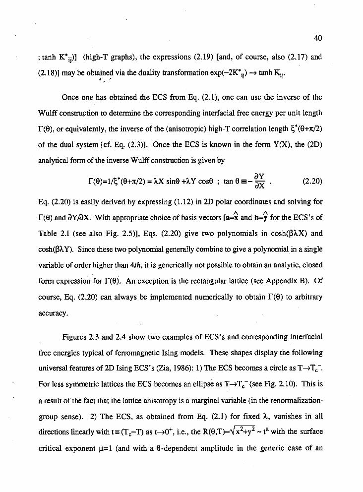
2.3 The ECS (left) and corresponding Wulff plot (right) of the diced lattice (Fig.

2 .5~) for equal, ferromagnetic couplings. 42

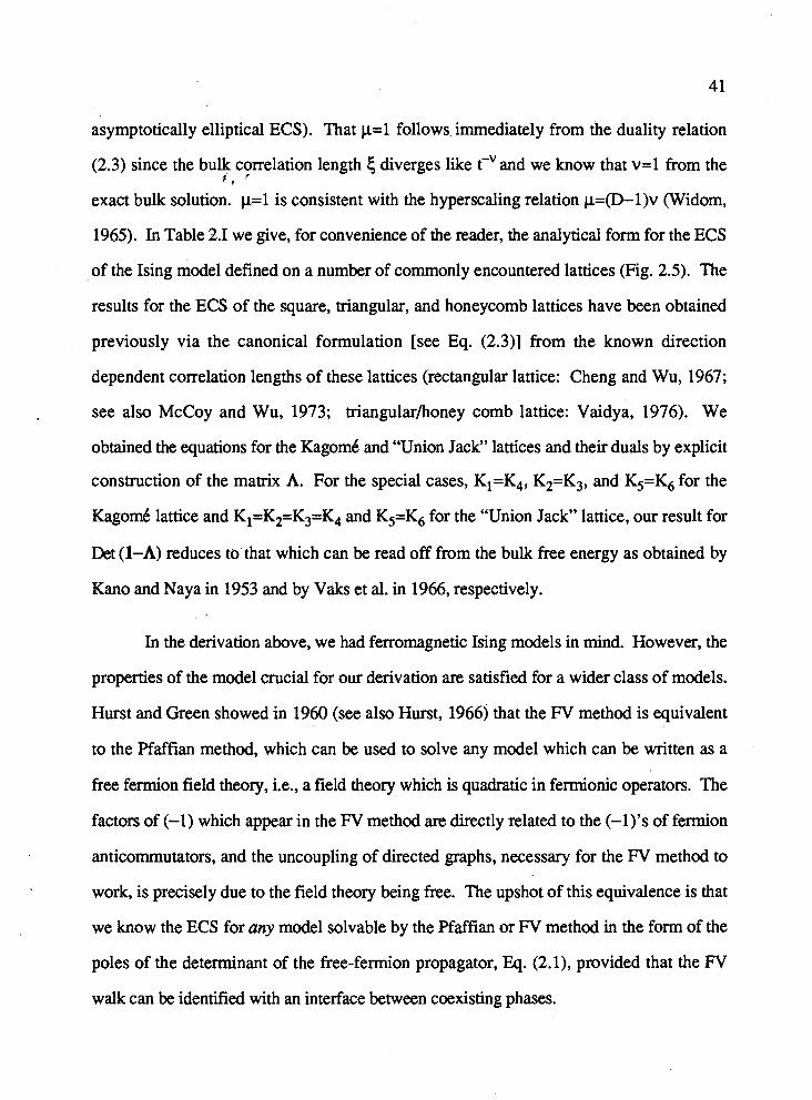
2.4 Same as Fig. 2.3 for the 4-8 lattice with ferromagnetic couplings K1=K2=K3=K4 and K5=K6 as indicated in Fig. 2.5d with K1/K5=3/2. 42

2.5 The lattices of Table 2.1 in duality pairs: 43

2.6 The eight vertex configurations of the eight-vertex model. 46

2.7 The antiferromagnetic sector of the free-fermion model, defined by the vertex

weights of Eq. (2.26), in the h-v plane of horizontal and vertical (electric)

fields. 5 1

2.8 An interface between two degenerate 2x1 phases of the antiferromagnetic

triangular Ising model. 53 $ r

I

2.9 The one-to-one correspondence between vertex configurations of the eight-

vertex model and composite elementary interfaces on the hexagonal lattice, 53

2.10 Equilibrium crystal shapes of the free-fermion model defined by the vertex weights of Eq. (2.25) at h=v=O and for various values of el/&: 55

2.1 1 The Feynman-Vdovichenko walker for the m o d i f i e d ' ~ ~ ~ model performs a

very simple walk on the honeycomb lattice; 5 8

2.12 The ECS of the modified KDP model (solid lines, left) and the corresponding

Wulff plot (right) for h=v=O. 59

3.1 Sketch of the thermal evolution of a ("type A") ECS of cubic symmetry. 63

3.2 An island excitation on an otherwise flat crystalline interface (atoms have been

coarse grained into bricks), 64

3.3 Top: The SOS model. The interface is represented by an array of stacks of

cubes. Bottom: A lattice-gas version of the interface. Overhangs, bubbles,

and handles are present. 66

3.4 The Wulff construction in the vicinity of a cusp (point A), 70

3.5 Perspective view of a fixed-8 cut through the ECS and its Wulff plot as

described in the text, 72

3.6 A strip of vicinal surface projected onto the xy plane, 75

3.7 Typical step configurations of the simple cubic Ising (100) interface; 78

3.8 This figure illustrates that the step cannot be chosen as a single non-self-

intersecting line without ambiguity, 82

3.9 Polar plots of the low-temperature series of y(8) at the temperatures indicated. 94

3.10 The facet shape at different temperatures, normalized to the centre-of-crystal

to centre-of-facet distance as obtained from the 1 l th order series for y(x) r

(dotted curvk) and the Legendre transform of the 5th order series for y(0)

(solid curve). 95

n 3.1 1 a.) The canonical series y(z ,N) for the step free energy and b.) the grand

canonical series y(0,N) for the facet shape, summed to the orders N indicated,

as a function of temperature. 96

3.12 Plots for the 3D Ising model of B(T)~(€I,N)~~~[C(T)/~FT], with C(T)=

-~(T~-T)" a i n y ( e , ~ y a ~ , and of C(T) versus temperature T for various

values of TR. 100

3.13 The normalized facet radius pf in the symmetry directions as a function of

temperature. 102

Trajectories of the two zeros of Det [1-A(kx,-iphX)] in the kx-plane for the

square lattice [cf. Eq. (A.6)] as X ranges from - to -. 107

Trajectories of the two zeros of Det [1-A(kx,-iphX)] in the z-plane for the

square lattice [cf. Eq. (A.6)] as X ranges from - to -. 108

The real zeros of Det [I-A(kx,-iphX)] for the square lattice in the z-plane as

a function of X. 108

Regions of nonconvergence (black squares) of A(kx,-iphX) in the kx-plane

for the square lattice at T=TJ2 for the values of X indicated, 1 09

Regions of nonconvergence (black squares) of A(kx,-iphX) in the Brillouin

zone for the square lattice at T& for the values of X indicated, 110

Trajectories of the two zeros of Det [1-A(kx,-iphX)] in the kx-plane for the

hexagonal lattice [cf. Eq. (A.6)] as X ranges from - to -. 112

Trajectories of the two zeros of Det [1-A(kx,-iphX)] in the z-plane for the

hexagonal lattice [cf. Eq. (A.6)] as X ranges from - to -. 113

xii

A.8 The real zeros of Det [1-A(k,,-ipm)] in the z-plane for the hexagonal lattice

as a function ofrX. t ,

113

A.9 Regions of nonconvergence (black squares) of A(k,,-iphX) in the k,-plane

for the hexagonal lattice at T=T& for the values of X indicated. 115/116

A. 10 Regions of nonconvergence (black squares) of A(k,,-iPU) in the Brillouin

zone for the hexagonal lattice at T=TJ2 for the values of X indicated. 116

E. 1 The vertical bonds of a step from (0,O) to (N,M) may be considered to be

distributed over N+l bins. 125

E.2 (a) The eight orientations of the L shape of diagram #16 (10 extra plaquettets).

(b) The possible straddling configurations of the L shape of orientation 1 for a

fixed realization of the step. (c) The possible straddling configurations of the

L shape of orientation 3 for a fixed realization of the step. (d) The vertical

bonds of the realization of the step shown stacked in their bins. 131

E.3 Fixed realizations of the diagram ( O--O ) in the 2D and 3D interpretations. 135

1. Introduction

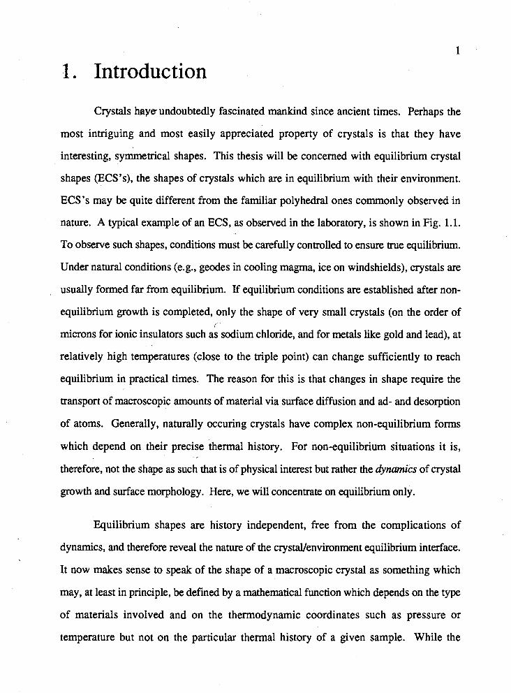
Crystals haye undoubtedly fascinated mankind since ancient times. Perhaps the

most intriguing and most easily appreciated property of crystals is that they have

interesting, symmetrical shapes. This thesis will be concerned with equilibrium crystal

shapes (ECS's), the shapes of crystals which are in equilibrium with their environment.

ECS's may be quite different from the familiar polyhedral ones commonly observed in

nature. A typical example of an ECS, as observed in the laboratory, is shown in Fig. 1.1.

To observe such shapes, conditions must be carefully controlled to ensure true equilibrium.

Under natural conditions (e.g., geodes in cooling magma, ice on windshields), crystals are

usually formed far from equilibrium. If equilibrium conditions are established after non-

equilibrium growth is completed, only the shape of very small crystals (on the order of I

microns for ionic insulators such as sodium chloride, and for metals like gold and lead), at

relatively high temperatures (close to the triple point) can change sufficiently to reach

equilibrium in practical times. The reason for this is that changes in shape require the

transport of macroscopic amounts of material via surface diffusion and ad- and desorption

of atoms. Generally, naturally occuring crystals have complex non-equilibrium forms

which depend on their precise thermal history. For non-equilibrium situations it is,

therefore, not the shape as such that is of physical interest but rather the dynamics of crystal

growth and surface morphology. Here, we will concentrate on equilibrium only.

Equilibrium shapes are history independent, free from the complications of

dynamics, and therefore reveal the nature of the crystal/environment equilibrium interface.

It now makes sense to speak of the shape of a macroscopic crystal as something which

may, at least in principle, be defined by a mathematical function which depends on the type

of materials involved and on the thermodynamic coordinates such as pressure or

temperature but not on the particular thermal history of a given sample. While the

FIG. 1.1. Electron micrographs of a small crystalite of lead approximately 6pm in diameter

at -300eC as prepared by Heyraud and Mttois (see Heyraud and Mttois, 1983). The vapour

pressure at this temperature is so low Torr) that pressure control is not important in this

case and the sample can simply be maintained in a high vacuum.

Top: Viewing the crystal along the [loo] direction: The large, slightly hexagonal (1 11)

facets are easily seen. The { 100) facets are also present but smaller and difficult to see.

Bottom: Viewing the crystal along the [I101 direction: The facets are flat and join the

curved parts of the shape smoothly.

These photographs are reproduced here with the permission of M. Wortis, to whom J. C.

Heyraud and J. J. MCtois kindly made these photographs available.

thermodynamics of ECS's has been understood nearly a century ago by Wulff, the

determination of &se shapes from the statistical mechanics of a microscopic Hamiltonian

has been of considerable interest only in recent years. This interest has been fueled on the

theoretical side mainly by the discovery of surface phase transitions (most notably the

roughening transition) and, on the experimental side, by technological advances which

make it possible to attain true equilibrium conditions under which to observe the shapes of

small crystals. The field has been very active over the last decade and several excellent

reviews cover these developments: Zia, 1984; Rottrnan and Wortis, 1984a; Abraham,

1486; van Beijeren and Nolden, 1987; Wortis, 1988; Zia, 1988. We shall, therefore, only

give such background as is needed for this thesis to be reasonably self-contained. During

the remainder of the Introduction, we will develop the fundamentals of ECS theory.

Further background will be provided at the beginning of each main Section.

1.1 The ECS as a classical variational problem and Wulff' s Theorem

A crystal can only be in equilibrium with another phase when the state of the system

crystal-plus-other-phase lies on a first-order coexistence c w e of the system's phase

diagram. We take our system to be contained in a box of volume VB. The box is in contact

with a heat bath whose temperature T is under our control. For simplicity and definiteness,

consider a pure substance X at gaslsolid coexistence, as shown in Fig. 1.2. The box

contains a fixed amount of X, enough so that after equilibrium has been reached the

pressure inside the box lies on the gaslsolid coexistence c w e , i.e., P=Po(T). The solid

and gas densities and, therefore, the volume of the crystal, V, are then determined and

fixed (see Fig 1.2). To keep the physics as simple as possible, we assume the box to be in

free fall so that we need not worry about the rather subtle effects of gravity (see, for $ f

example, Avron et al., 1983; Zia and Gittis, 1987; Avron and Zia, 1988). Further, we

assume the crystal to be freely floating in the interior of the box, far away from the walls of

the container, so that we need not worry about substrate geometries and other

complications due to the presence of the walls of the box. The important point now is that

the bulk free energies of the solid and gas and the free energy coming from the walVgas

interactions are fmed. The only way in which the system can lower its free energy to attain

true equilibrium is to change the shape of the crystal, so as to minimize the total free energy A

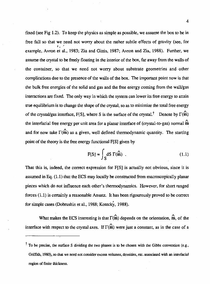
of the crystaVgas interface, F[S], where S is the surface of the crystaLt Denote by T(m) A

the interfacial free energy per unit area for a planar interface of (crystal-to-gas) normal m A

and for now take T(m) as a given, well defined thermodynamic quantity. The starting

point of the theory is the free energy functional F[S] given by

That this is, indeed, the correct expression for F[S] is actually not obvious, since it is

assumed in Eq. (1.1) that the ECS may locally be constructed from macroscopically planar

pieces which do not influence-each other's thermodynamics. However, for short ranged

forces (1.1) is certainly a reasonable Ansatz. It has been rigourously proved to be correct

for simple cases (Dobrushin et al., 1988; ~oteck;, 1988).

A What makes the ECS interesting is that T(k) depends on the orientation, m, of the

A interface with respect to the crystal axes. If T(m) were just a constant, as in the case of a

' To be precise, the surface S dividing the two phases is to be chosen with the Gibbs convention (e.g.,

Griffith, 1980), so that we need not consider excess volumes, densities, etc. associated with an interfacial

region of finite thickness.

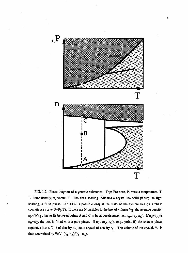
FIG. 1.2. Phase diagram of a generic substance. Top: Pressure, P, versus temperature, T.

Bottom: density, n, versus T. The dark shading indicates a crystalline solid phase; the light

shading, a fluid phase. An ECS is possible only if the state of the system lies on a phase

coexistence curve, P=PO(T). If there are N particles in the box of volume VB, the average density,

nO=N/VB, has to lie between points A and C to be at coexistence, i.e., n g ~ [nA,nC]. If no=nA or

no=nc, the box is filled with a pure phase. If no€ (nA,nC), (e.g., point B) the system phase

separates into a fluid of density n~ and a crystal of density nc. The volume of the crystal, V, is

then determined by V=VB(no-nA)/(nC-nA).

fluid/fluid interface, it follows from symmetry that the equilibrium shape would be a A

sphere. The anis9popy of T(m) for a crystalbything interface results in a non-spherical

equilibrium shape which assigns as little area as possible to high-energy orientations and as

much area as possible to low-energy orientations. This weighted assignment of areas takes

place in such a way as to minimize F[S] subject to the constraint that the volume, V[S],

enclosed by the surface S remain fixed. This statement, with F[S] of the form (1.1), was

already asserted in 1885 by P. Curie. Incorporating the constant volume constraint via a

Lagrange multiplier (D-1)h (defined for later convenience in terms of D, the spatial

dimension of the bulk crystal), the ECS describes a surface S for which the functional

is stationary. In case of multiple solutions, the ECS corresponds to the one for which F[S]

is smallest. [The Euler-Lagrange equations of (1.2) are generally nonlinear.]

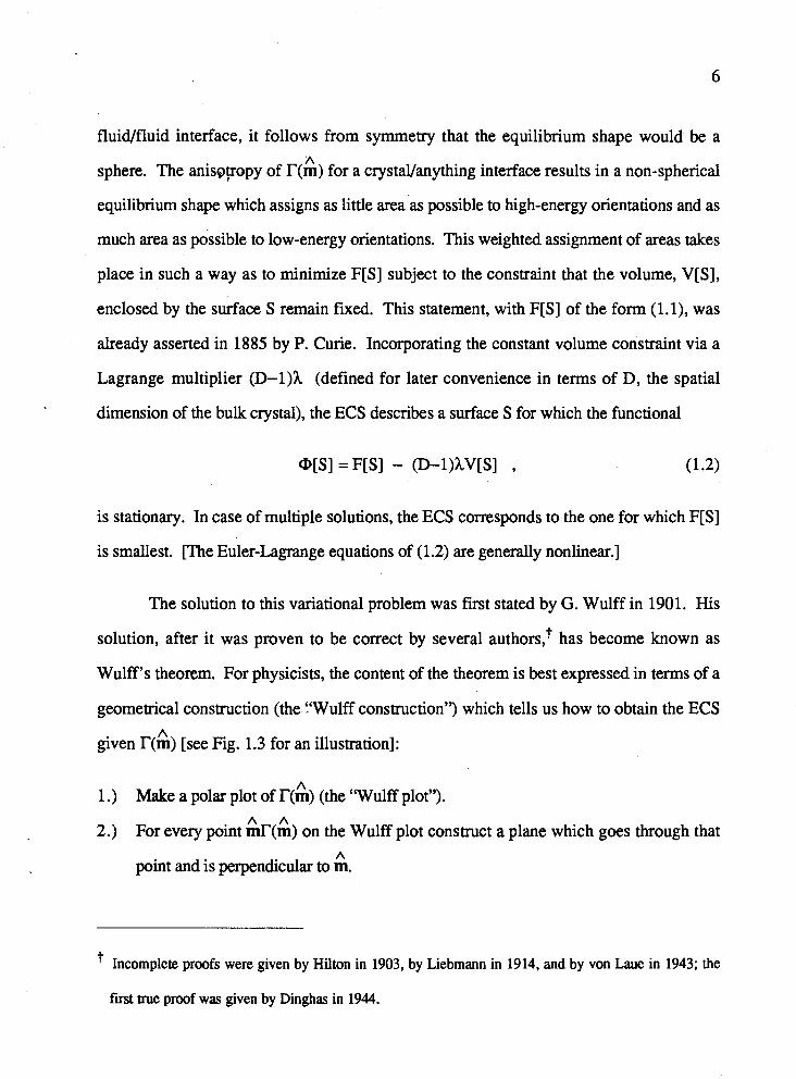
The solution to this variational problem was first stated by G. Wulff in 1901. His

solution, after it was proven to be correct by several authors: has become known as

Wulff's theorem. For physicists, the content of the theorem is best expressed in terms of a

geometrical construction (the. f'wulff construction") which tells us how to obtain the ECS A

given T(m) [see Fig. 1.3 for an illustration]:

1 .) Make a polar plot of r(A) (the "Wulff plot"). A A

2.) For every point mlJm) on the Wulff plot construct a plane which goes through that A

point and is perpendicular to m.

Incomplete proofs were given by Hilton in 1903, by Liebmann in 1914, and by von Laue in 1943; the

first m e proof was given by Dinghas in 1944.

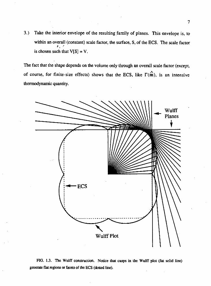
3.) Take the interior envelope of the resulting family of planes. This envelope is, to

within an overall (constant) scale factor, the surface, S, of the ECS. The scale factor t f

is chosen such that V[S] = V.

The fact that the shape depends on the volume only through an overall scale factor (except, A

of course, for finite-size effects) shows that the ECS, like T(m), is an intensive

thermodynamic quantity.

4 Wulff Planes

\\ Wulff Plot

FIG. 1.3. The Wulff construction. Notice that cusps in the Wulff plot (fat solid line)

generate flat ~ g i o n s or facets of the ECS (dotted line).

Since the Wulff theorem is the cornerstone of this thesis, we will now motivate it

and then present i$sf proof (a physicist's version) as given by Herring in 1% 1. Consider A

first the case of a fluid/fluid interface, i.e, T(m)=To=constant. By symmetry we may

restrict ourselves to spherest of some yet-to-be-determined radius R. A trivial calculation

shows that hR = To

locally stationarizes the functional iP[S] and that the corresponding sphere is the unique

spherically symmetric minimum of F[S]. Since To is just the surface tension of the

interface, it follows from mechanical equilibrium that (P2-Pl)/2=T&, where P2 and P1

are the hydrostatic pressures inside and outside the sphere, respectively. Thus, we may

make the identification h=(P2-P1)/2.

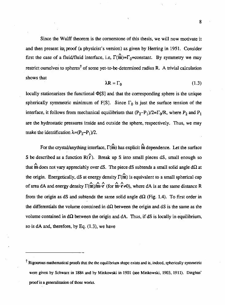
For the crystallanything interface, T(C) has explicit & dependence. Let the surface A

S be described as a function R(r). Break up S into small pieces dS, small enough so A

that m does not vary appreciably over dS. The piece dS subtends a small solid angle dQ at A

the origin. Energetically, dS at energy density T(m) is equivalent to a small spherical cap A A h A A

of area dA and energy density T(m)/m*r (for merd)), where dA is at the same distance R

from the origin as dS and subtends the same solid angle dR (Fig. 1.4). To first order in

the differentials the volume contained in dQ between the origin and dS is the same as the

volume contained in dQ between the origin and dA. Thus, if dS is locally in equilibrium,

so is dA and, therefore, by Eq. (1.3), we have

Rigourous mathematical proofs that the the equilibrium shape exists and is, indeed, spherically symmetric

were given by Schwan in 1884 and by Minkowski in 1901 (see Minkowski, 1903, 1911). Dinghas'

proof is a generalization of those works.

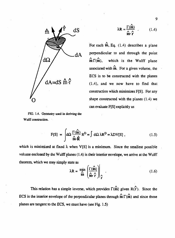
FIG. 1.4. Geometry used in deriving the

Wulff construction.

A For each m, Eq. (1.4) describes a plane

perpendicular to and through the point

PI'(&, which is the Wulff plane A

associated with m. For a given volume, the

ECS is to be constructed with the planes

(1.4), and we now have to find that

construction which minimizes F[S]. For any

shape constructed with the planes (1.4) we

can evaluate F[S] explicitly as

which is minimized at fixed h when V[S] is a minimum. Since the smallest possible

volume enclosed by the Wulff planes (1.4) is their interior envelope, we arrive at the Wulff

theorem, which we may simply state as

A A This relation has a simple inverse, which provides T(m) given R(r). Since the

A h ECS is the interior envelope of the perpendicular planes through m T(m) and since these

planes are tangent to the ECS, we must have (see Fig. 1.5)

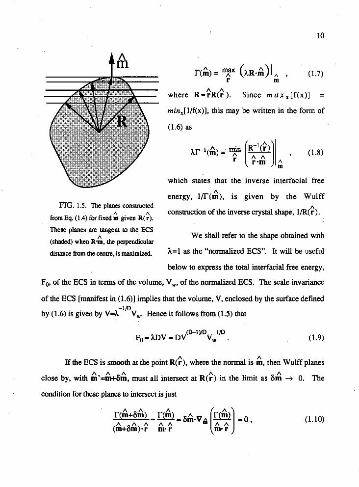
FIG. 1.5. The planes constructed A A

from Eq. (1.4) for fixed m given R(r).

These planes are tangent to the ECS A

(shaded) when Rm, the perpendicular

distance from the centre, is maximized.

A r(m) = 7 (XRA) I A ,

r m (1.7)

A where R= rR(r ). Since m a x , [f(x)] =

min,[l/f(x)], this may be written in the form of

(1.6) as

which states that the inverse interfacial free A

energy, l/T(m), is given by the Wulff A

construction of the inverse crystal shape, l/R(r ) .

We shall refer to the shape obtained with

h=l as the "normalized ECS". It will be useful

below to express the total interfacial free energy,

Fo, of the ECS in terms of the volume, V,, of the normalized ECS. The scale invariance

of the ECS [manifest in (1.6)] implies that the volume, V, enclosed by the surface defined -lP

by (1.6) is given by V=h V,. Hence it follows fn>m (1.5) that

If the ECS is smooth at the point R($), where the normal is &, then Wulff planes A h A A A

close by, with mY=m+6m, must all intersect at R(r) in the limit as 6m + 0. The

condition for these planes to intersect is just

A A provided T(m) is differentiable.? Since (1.10) must hold for any Sm, we have

P ' A A A A A VA [%)= $&A-[r-m (me r)]) r(m) = 0 ,

m-r

A A which defines r as a function of m, and is just the analytical form of the mink(.) function

A A A A of Eq. (1.6) in the case of differentiable l?(m). Decomposing R[r (m)]=R(m) into vectors

A parallel and perpendicular to m and using (1.1 I), we may write the ECS as a parametric

A function of m , i.e,

for those parts of the ECS constructed from differentiable parts of the Wulff plot.

In our derivation above, we found a particular solution for which F[S] is stationary.

However, it is far from obvious that there are no other solutions for which F[S] is smaller A

yet. If we represent the ECS as a function R(r) as in the preceeding discussion, Eq. (1.2)

may be written as

Variations R+R+GR induce variations in O which must be zero for a stationary solution. A

When T(m) is differentiable, our argument for the derivation of the Wulff construction

amounts to nothing more than to writing these variations as (Zia, 1984)

A The transverse gradient, V&, is defined by [Vp f(m)lc = (6cV-(c(v/(2) (

a = ~c~ ( a 6) with (=-\/z. In two-dimensional polar coordinates, Vfh = 6- . acv ae

Evidently, 6@[S] = 0 when Eqs. (1.6) and (1.11) are satisfied. Clearly, however, there

may be other solutions in which the sum of the two terms in the integrand of (1.14) is zero P , '

but the individual terms are not. A priori, it is not even clear that the ECS can be A

represented by a single valued function R(r). Furthermore, our tacit assumption that the

interface may be represented by equivalent infinitesimal spherical caps of a common centre

of curvature does, in principle (while being physically very plausible and, as it turns out,

correct), also require proof.

Dinghas' ingenious proof and its successive refinements and extensions (Herring,

1953; ~ a ~ l o r ~ , 1974, 1978) put all these worries to rest by proving that the Wulff solution

gives the absolute minimum of F[S] at fixed volume. In their most general and powerful

form, the proof and, indeed, the statement of the theorem itself, requires the technology of

geometric measure theory (Taylor, 1974). We will content ourselves here with a more

simple version.

At the-heart of the proof of the Wulff theorem lies the Brunn-Minkowski inequality

(e.g., Minkowski, 191 1; Federer, 1969), which states the following (see Fig. 1.6): Let the

"bodies" Bl and B2 be nonempty subsets of RD having volumes V1 and V2, respectively.

Let Xce B2 and call it the centre of By Define a third body B as the subset of RD which is

swept out with B2 as the centre of B2 is placed at all points of B1 keeping fixed the

orientation of both B1 and B2. If we denote the volume of by ?, then the theorem states

with the equality holding if and only if B1 and B2 are geometrically similar.

Taylor (1978) will tell you how to catch fish with the Wulff construction!

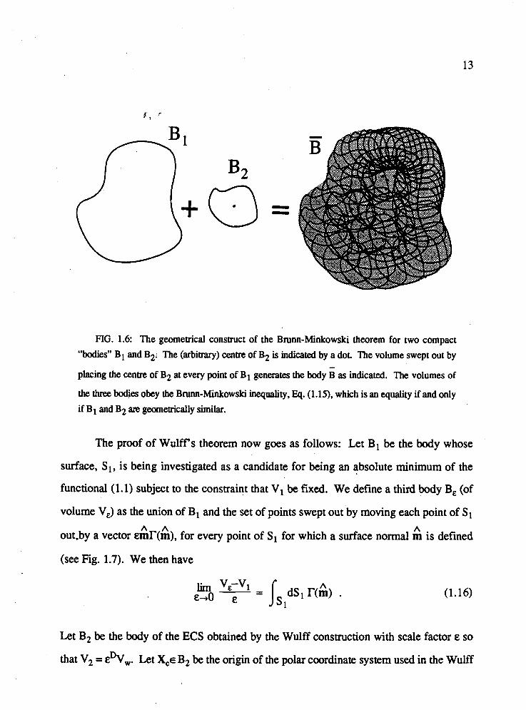
FIG. 1.6: The geometrical construct of the Brunn-Minkowski theorem for two compact

"bodies" B1 and B2. The (arbitrary) centre of B2 is indicated by a dot. The volume swept out by

placing the centre of B2 at every point of B1 generates the body as indicated. The volumes of

the three W e s obey the Brum-Minkowski inequality, Eq. (1.15), which is an equality if and only

if B1 and B2 are geometrically similar.

The proof of Wulff's theorem now goes as follows: Let B1 be the body whose

surface, S1, is being investigated as a candidate for being an absolute minimum of the

functional (1.1) subject to the constraint that V1 be fixed. We define a third body B, (of

volume V,) as the union of B1 and the set of points swept out by moving each point of S1 A h A

out.by a vector &mT(m), for every point of S1 for which a surface normal m is defined

(see Fig. 1.7). We then have

Let B2 be the body of the ECS obtained by the Wulff construction with scale factor E so

that V2 = E-,. Let XCc B2 be the origin of the polar coordinate system used in the Wulff

construction, and form the body B as described above. Since the Wulff construction A A

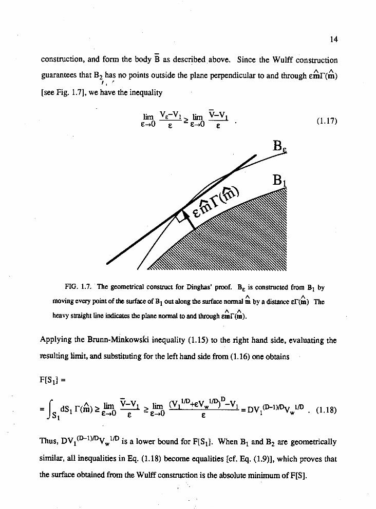
guarantees that B2 has no points outside the plane perpendicular to and through &mT(m) + , '

[see Fig. 1.71, we have the inequality

FIG. 1.7; The geometrical construct for Dinghas' proof. B, is constructed from B1 by A A

moving every point of the surface of B1 out along the surface normal m by a distance C(m) The A A

heavy straight line indicates the plane normal to and through ~mT(m).

Applying the Brunn-Minkowski inequality (1.15) to the right hand side, evaluating the

resulting limit, and substituting for the left hand side from (1.16) one obtains

Thus, D V ~ ( * ' ) ~ V , ' ~ is a lower bound for FISI]. When B1 and B2 are geometrically

similar, all inequalities in Eq. (1.18) become equalities [cf. Eq. (1.9)], which proves that

the surface obtained from the Wulff construction is the absolute minimum of F[S].

The fact that the Wulff construction gives the ECS as the interior envelope of planes

strongly suggests that a Legendre transform may be involved (e.g., Callen, 1960). That * , '

this is, indeed, the case was first recognized by Andreev in 1982 (81 years after Wulff!). A

The fact that R(r) is the Legendre transform of ~ ( 4 ) is most clearly visible when the ECS

is described in Cartesian coordinates as z(x), x=(x,y). It is then natural to describe the az orientation of the interface in terms of its slope p = - and in terms of the interfacial free ax

energy per unit projected area in the x-y plane, given by f(p) = I'(&)ql+p2, with &(p) =

(-p,, -py, 1 ) / d G 2 . Transcribing Eq. (1.6) to Cartesian coordinates, one obtains

with

q and p are conjugate variables related byt

and

provided f(p) is differentiable at p. Eqs. (1.20-22) clearly express f (q ) and f(p) as

Legendre-transform-conjugate pairs.

Since the Legendre transform is nothing more than a change of variables, the

normalized ECS, as obtained from the Wulff construction, is itself a free energy surface!

This is, perhaps, the most astonishing result of ECS theory. The Wulff plot describes the A

anisotropic interfacial free energy in terms of the independent variable m (or p), whereas

the ECS does the same in terms of the conjugate variable : (or q). That the ECS and the

Eq. (1.21) may be recognized as a &anscription of (1.12) by using the fact that [(V&, = -m a -

ap '

interfacial free energy are different representations of the same physical quantity is already

apparent from the Wulff construction, itself, since the Wulff plot may be reconstructed f f

from the ECS via the inverse relation (l.8).? Legendre transform conjugacies are A A

ubiquitous in thermodynamics, and the conjugacy between T(m) and R(r) is precisely

analogous to any other such conjugacy commonly encountered. For example, the

Helmholtz free energy density of a magnetic system, f(m), gives the free energy in terms of

the system's magnetization density, m. Via the Legendre transform, one obtains the

corresponding Gibbs free energy density g(h) as g(h)=f(m)-mh, with -m=ag/ah and

h=af/am, which describes the system in terms of the conjugate field variable h (which in

this case is literally the applied field). To remind ourselves of the analogy with such more A A

familiar cases, we call m (or p) the density variable, and r (or q), thefield variable.

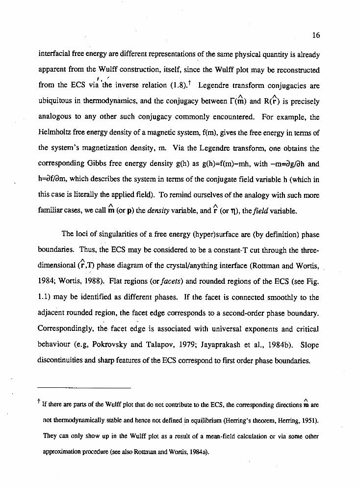
The loci of singularities of a free energy (hyper)surface are (by definition) phase

boundaries. Thus, the ECS may be considered to be a constant-T cut through the three- A

dimensional ( r ,T) phase diagram of the crystaVanything interface (Rottman and Wortis,

1984; Wortis, 1988). Flat regions (or facets) and rounded regions of the ECS (see Fig.

1.1) may be identified as different phases. If the facet is connected smoothly to the

adjacent rounded region, the facet edge corresponds to a second-order phase boundary.

Correspondingly, the facet edge is associated with universal exponents and critical

behaviour (e.g, Pokrovsky and Talapov, 1979; Jayaprakash et al., 1984b). Slope

discontinuities and sharp features of the ECS correspond to first order phase boundaries.

A If there are parts of the Wulff plot that do not contribute to the ECS, the corresponding directions lo are

not thermodynamically stable and hence not defined in equilibrium (Herring's theorem, Herring, 1951).

They can only show up in the Wulff plot as a result of a mean-field calculation or via some other

approximation procedure (see also Roman and Wortis, 1984a).

17

1.2 Formulations of Statistical Mechanics: Canonical and Grand Canonical Descriptions of the ECS

4 ' ' A

In the previous section we took the interfacial free energy per unit area, T(m), as a

given thermodynamic quantity. In this Sub-section, we discuss the thermodynamic A

definition of T(m) and, from that, give a microscopic definition in terms of a Boltzmann

sum (trace) over a "canonical" ensemble of microscopic configurations. We will then make A A

use of the Legendre transform duality between the ECS, R(r), and T(m) to formulate the

ECS directly in terms of a "grand canonical" trace.

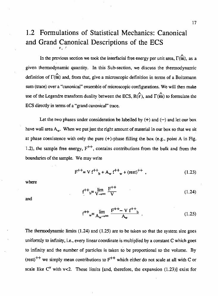
Let the two phases under consideration be labelled by (+) and (-) and let our box

have wall area A,. When we put just the right amount of material in our box so that we sit

at phase coexistence with only the pure (+)-phase filling the box (e.g., point A in Fig.

1.2), the sample free energy, I ? + , contains contributions from the bulk and from the

bundaies of the sample. We may write

where

and

The thermodynamic limits (1.24) and (1.25) are to be taken so that the system size goes

uniformly to infinity, i.e., every linear coordinate is multiplied by a constant C which goes

to infinity and the number of particles is taken to be proportional to the volume. By

(rest)* we simply mean contributions to F* which either do not scale at all with C or

scale like CV with vc2. These limits [and, therefore, the expansion (1.23)] exist for

sufficiently short ranged microscopic forces (e.g., Fisher and Caginalp, 1977; Caginalp

and Fisher, 1979). Eqs. (1.24) and (1.25) define the bulk free energy, fHb , and the wall f f ,'

free energy per unit area, fH, , respectively. Similarly, we define ib and f-, for the

(-1 phase. .

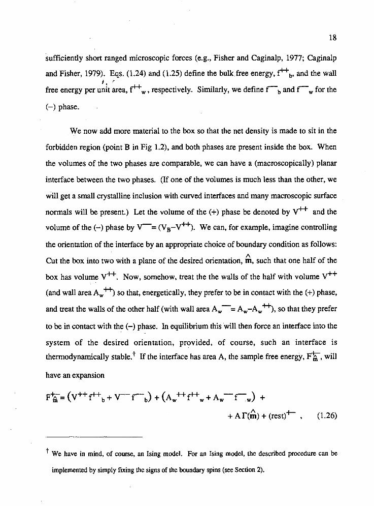
We now add more material to the box so that the net density is made to sit in the

forbidden region (point B in Fig 1.2), and both phases are present inside the box. When

the volumes of the two phases are comparable, we can have a (macroscopically) planar

interface between the two phases. (If one of the volumes is much less than the other, we

will get a small crystalline inclusion with curved interfaces and many macroscopic surface

normals will be present.) Let the volume of the (+) phase be denoted by V++ and the

volume of the (-) phase by T= (VB-v*). We can, for example, imagine controlling

the orientation of the interface by an appropriate choice of boundary condition as follows: A

Cut the box into two with a plane of the desired orientation, m, such that one half of the

box has volume v*. Now, somehow, treat the the walls of the half with volume V++

(and wall area A,? so that, energetically, they prefer to be in contact with the (+) phase, -

and treat the walls of the other half (with wall area A, = A,-A,?, so that they prefer

to be in contact with the (-) phase. In equilibrium this will then force an interface into the

system of the desired orientation, provided, of course, such an interface is

thermodynamically stable.+ If the interface has area A, the sample free energy, a, will

have an expansion

We have in mind, of course, an Ising model. For an Ising model, the described procedure can be

implemented by simply fixing the signs of the boundary spins (see Section 2).

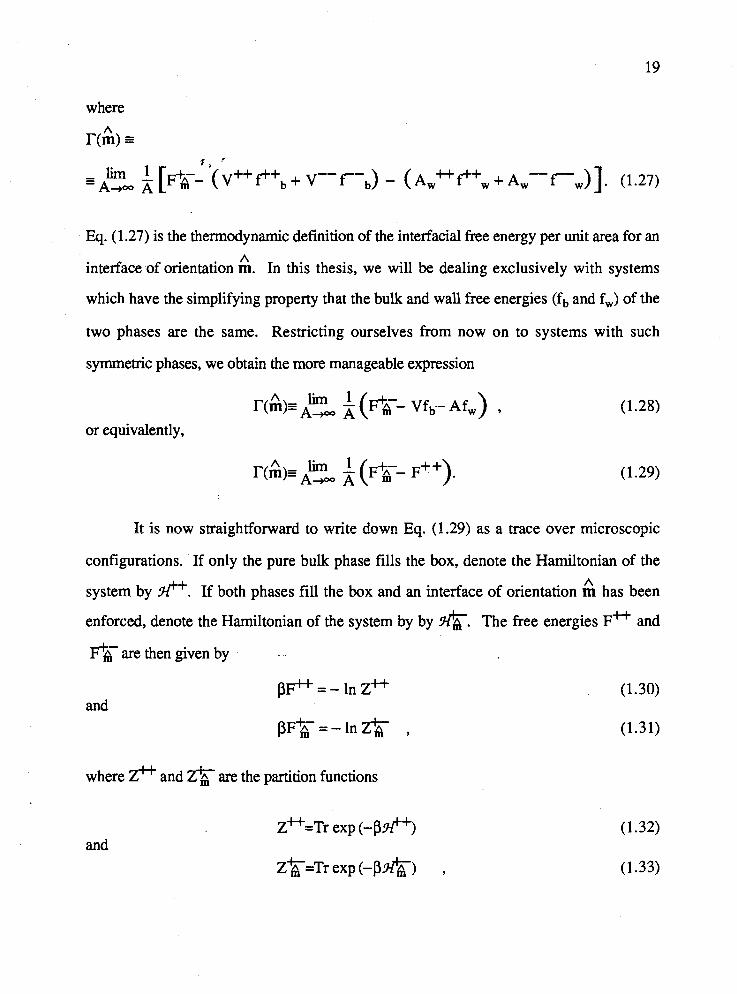
where A

r(m) n P , '

- - lim [F%-- ( v + + P b + v--T-~) - (A,* pw + A W - r w ) ] . (1.27) -A+- A

Eq. (1.27) is the thermodynamic definition of the interfacial free energy per unit area for an A

interface of orientation m. In this thesis, we will be dealing exclusively with systems

which have the simplifying property that the bulk and wall free energies (fb and f,) of the

two phases are the same. Restricting ourselves from now on to systems with such

symmetric phases, we obtain the more manageable expression

or equivalently,

It is now stralghtforwzrd to write dowr? Eq. (1.29) as a trace over microscopic

configurations. If only the pure bulk phase fills the box, denote the Hamiltonian of the

system by c. If both phases fill the box and an interface of orientation has been

enforced, denote the Hamiltonian of the system by by &. The free energies F* and

F$& are then given by

and

where and a are the partition functions

zH=Tr exp (-p#+) and

Z==T~ exp (-P&) ,

where P=(kB~)-', with kB Boltzmann's constant. In terms of these partition functions,

Eq. (1.29) becomes C , '

We shall regard (1.34) as the "canonical" description of the interfacial free energy, because A

the trace is carried out at fured macroscopic orientation m in analogy with the fixed density

or magnetization constraint of more familiar canonical ensembles. Correspondingly, we A

regard the description of the ECS which instructs us first to calculate T(m) via (1.34) and

then to obtain the ECS via the Wulff construction, to be the "canonical" description of the

equilibrium crystal shape problem. So far we have put "canonical" and "grand canonical"

in quotation marks to emphasize that we do not mean the standard canonical and grand

canonical ensemble of particles. Since from now on we will only speak of ensembles of

interfaces in this thesis, we will drop the quotes.

Eqs. (1.20) and (1.22) tell us how to arrive at a grand canonical description of the

ECS. Substituting the definition of r(A), Eq. (1.34), into the definition of pT(q), Eq.

(1.20), we obtain

where Axy Ad= Since we can expect the term Tr exp [ - ~ ( e - q * p ( h ) ~ ~ ~ ] to be

a sharply peaked function of h in the limit A,+.. (an explicit example will be given in

Section 2), we can extend the trace of (1.35) to a trace over a grand canonical ensemble of

systems. Each member of this ensemble is contained in a box of base area Axy on which

boundary conditions have been imposed to enforce a macroscopically planar interface of A

orientation m as described above. Each member has Hamiltonian *and may be labelled

by its orientation A.t Summing over this ensemble, we obtain the grand canonical

expression for the ECS, . f . '

where p(fh) is the slope of the plane used in enforcing the boundary conditions for each

member of the ensemble. The field term, exp[Pq*p(fh)~,,], is a fugacity for the slope,

p(fh), and, therefore, controls the orientation of the interface.

It is sometimes useful to enlarge the ensemble further to include systems which

have arbitrary macroscopic interfaces (of macroscopically planar topology but not

necessarily planar) running across the box (we can, for example, imagine defining the

boundary conditions by dividing the walls of the box into two arbitrary, simply connected

parts). Denoting microscopic quantities from now on by script letters, we replace the field

term, q*pAxy, with q*jA p(x)dx dy = -(qxP + qyf )*jsfhd(. (When the interface is XY

forced to have edges which all lie in a plane of slope p, the replacement becomes an

identity, since the integral of& over a closed surface vanishes.) In this larger ensemble

we may, thus, write

If we want this ensemble to contain interfaces of large slopes lpl, the ratio (box height)/Ky is to be

chosen sufficiently large so that the projected area of the interface remains Axy, i.e., so that steep

interfaces do not "cut off' comers of the box.

where the notation {fh) indicates that arbitrary interfaces are included in the ensemble. Eq.

(1.38) is particularly useful when pure interface models (such as the SOS model) are being

considered, since (1.38) then allows an unrestricted sum over interface configurations

(e.g., Jayparakash et al., 1983). Since in our box geometry f *lSthdS = Axy for any

configuration, we may bring pT(q)=ln{exp[PAxy?'(q)] }/Axy to the right hand side of Eq.

(1.38) and write

which provides a coordinate independent grand canonical description of the ECS in which

R(+) appears as an implicitly determined quantity.

Eq. (1.38) gives the correct expression, Eq. (1.22), for the expectation value of the

slope:

The fluctuations in the slope are calculated as

where Kij is the curvature tensor of the normalized ECS (for a more complete discussion

on this tensor, see Zia, 1984; Akutsu and Akutsu, 1987a). The eigenvalues of Kij are l/R1

and 1/R2, where R1 and R2 are the principal radii of curvature. Therefore, where the ECS

has well defined curvature with R1 and R2 finite, the fluctuations in the slope go to zero # t

like l/Axy in the thermodynamic limit AXy+- and the grand canonical trace does, indeed,

select a sharp slope p according to the Wulff prescription (1.40). At sharp edges and

corners corresponding to first order surface phase coexistence, Kij is defined arbitrarily

close to the discontinuity and the fluctuations in the slope vanish in the thermodynamic

limit. Fluctuations would presumably be divergent at a second order (surface) critical

feature which has divergent radii of curvature. For lattice gas models, bulk coexistence

ends in a critical point at T=T,. Thus, as T, is approached in these models, the interfacial

free energy goes to O+ since the critical point may be characterized by unbounded

proliferation of interfacial area. Correspondingly, the normalized ECS, and, hence, the

principal radii of curvature, shrink to zero, so the fluctuations become divergent when the

critical point is approached, as we would expect.

1.3 Organization and Motivation

In the remhinder of this thesis we shall apply the concepts developed above to two

model calc~lations.~ In Section 2, we derive new exact solutions for the ECS's of two-

dimensional (2D) free-fermion models. These models include planar Ising models, and

also the modified KDP model which is not in the Ising universality class. In Section 3, we

focus on the thermal evolution of the equilibrium facet shape associated with the ECS of the

three-dimensional (3D) Ising model. We will derive low-temperature expansions for the

facet shape and its conjugate quantity, the anisotropic step free energy per unit length, i.e.,

the free energy associated with the creation of a single step on an otherwise flat crystal

surface. These expansions are naturally structured as perturbation expansions about the

exact result for the 2D square Ising model derived in Section 2. To date our low

temperature expansion is the only analytical calculation of the facet shape and step free

energy for a full interface model, i.e., a model which includes overhanging and bulk

excitations.

A unifying motivation for much of the work presented in this dissertation was the

following remarkable fact, which was first pointed out by van Beijeren and Nolden, and

also by Akutsu and Akutsu (1987b), in 1987, and will be derived in Section 3: Whenever

the facet edge is a second order phase boundary, it follows from the geometry of the Wulff

construction that the conjugacy between the ECS and the interfacial free energy per unit

area contains a precisely analogous conjugacy between the equilibrium facet shape and the

step free energy per unit length. This means that we may think of facets as 2 0 ECS's

which are embedded in the surface of a 30 ECS!

Sections 2 and 3 are adaptations to thesis format of research articles either already published (Holzer and

Wortis, 1989; Holzer, 1990a) or submitted for publication (Holzer, 1990b).

25

2. A General, Exact Solution for Equilib- rium Crystal Shapes in Two Dimensions for Free-Fertn'ion Models

2.1 Introductory Remarks

As a first application of the concepts discussed in Section 1, we will now derive an

exact solution for the ECS's of 2D planar Ising models. This solution immediately

generalizes to the somewhat larger class of so-called free-fermion models, which includes

non-Ising models and is the class of all models for which the bulk free energy may be

found exactly by the ~e~nman*-~dov ichenko (FV) method (Feynman, 1972;

Vdovichenko, 1965; see also Landau and Lifshitz, 1968; Morita, 1986) [or equivalently by

the Pfaffian method (Temperley and Fisher, 1961; Kasteleyn, 1961, 1963; see also McCoy

and Wu, 1973)l.

There are a number of reasons to study 2D Ising models: The Ising model in zero

magnetic field and below the bulk transition temperature (Tc) is the simplest model

describing a full two-phase system [as opposed to a pure "interface" model such as the

SOS model (e.g., Leamy et al., 1975; the SOS model is'also discussed in Section 3)]. The

two-dimensional (2D) Ising model is particularly interesting for at least two reasons: 1.)

Exact solutions are possible (Onsager, 1944) and 2.) as we shall see in section 3, these

exact solutions are valuable in approximating the shapes of facets of 3D Ising ECS's.

Since some real crystals, such as noble gas crystals, may possibly be approximated by an

appropriate 3D Ising model, 2D Ising ECS's may also have some relevance to the analysis

Feynman's solution for the bulk free energy of the Ising model predates Vdovichenko's (see Sherman,

1960) but was apparently not published until 1972. His solution is only slightly different from

Vdovichenko's.

of experimental facet-shape data. Finally, we mention, that prior to this work, exact ECS's

were known (from calculations conceptually completely different from ours) for the 4 , '

rectangular (Rottman and Wortis, 1981; Avron et al., 1982; Zia and Avron, 1982),

triangular and honeycomb lattices (Zia, 1986) only.?

Our calculation is formulated in the grand canonical description and makes use of an

exact mapping of the interface onto a FV "random" walker. This mapping makes possible

the exact evaluation of the grand canonical trace in the thermodynamic limit. Before

presenting the derivation, let us first state the simple solution, so it will clear what our aim

is: If the "momentum-space" FV lattice-walk matrix for a lattice L* (the dual of the direct

lattice L) is denoted by A(kx, ky), then the ECS for the dual model on L, represented in

Cartesian coordinates as Y(X), is given by

where {o) denotes the set of Boltzmann weights associated with the steps of the lattice

walk. The matrix A is a finite dimensional qxq matrix, where q is even and, in the

simplest cases, just equal to the coordination number of the lattice. Since the bulk partition

function of free-fermion models can be expressed in terms of an integral of the form

jdkxdky lnDa(1-A) [e.g., Landau and Lifshitz, 1968 and also below], the ECS for

these models may, in fact, be read off from the analytic form of the bulk free energy!

The FV method and its refinements have a venerable history. The root of the FV

method may be considered to be an unpublished conjecture by Feynman which was proved

by Sherman in 1960 (the Sherman theorem, see also Sherman, 1963; Burgoyne, 1963).

In the symmetry directions, the interfacial free energies for these lattices were fist published by Fisher

and Ferdinand in 1%7.

Feynman re-interpreted the seminal work of Kac and Ward (1952) on a combinatorial

solution of the Ising model in terms of an identity between lattice-path sums and the 4 ' -

graphical expansion of the Ising model. Making implicit use of the Sherman theorem,

Vdovichenko gave an elegant, intuitive solution to the Onsager problem in 1965. The first

application of these methods to Ising interfaces was recently reported by Calheiros,

Johannesen, and Merlini in 1987. The FV has now been textbook material (notably

Landau and Lifshitz, 1968) for some twenty years but appears not to be as well and widely

appreciated as perhaps it should be. We shall explain the method in detail below.

The remainder of this Section is organized as follows: In Sub-section 2.2, we

derive equation (2. I), discuss its range of validity and give some examples of previously

unknown Ising ECS's. In Sub-section 2.3, we explore, in some detail, a pedagogical

example of a non-Ising case for which Eq. (2.1) is also valid. We apply the FV method to

the free-fermion cases of the eight-vertex model (Fan and Wu, 1969,1970; Sutherland,

1970). The coexisting phases of the model are identified, and Eq. (2.1) is shown to give

the correct ECS of the corresponding dual models even for the non-Ising case of the

modified KDP model (Wu, 1967,1968).

2.2 Derivation

For definiteness consider an Ising model with ferromagnetic interactions. The

generalization to other free-fexmion models will be made at the end of this Sub-section. Let

the 2D Ising system be defined on a rectangular strip R (our "box") of a planar lattice L,

i.e., a lattice with non-crossing bonds. The strip l2 has a geometric dual, the strip R* of A

the dual lattice L*. Without loss of generality, we take the lattice to have basis vectors x A

and y, and we align the strip with the y-axis. (It is always possible to choose a coordinate

system in which the basis vectors of the lattice are orthogonal unit vectors.) We take the

width of R* to be N and think of the length of R* as finite but tending toward infinity Z 7

(Fig. 1). At zero mhgnetic field and T*, a phase of predominantly "up" (+) spins can

coexist with a phase of predominantly "down" (-) spins. The microscopic configurations

of the system can of course be described in terms of the spins on LR; but, in the present

context it is much more useful to think in terms of the bonds of R* dual to the "broken"

bonds of R, which connect spins of opposite sign (see Fig. 2.1). We consider these bonds A

to be elementary microscopic interfaces of microscopic normal m which we take to point

from - to +. If the coupling between spins at sites i and j of R is qj, the creation of an

elementary interface between them costs energy 2&@ and is, therefore, associated with a

Boltzmann factor of wij=exp(-2qj).

A macroscopic interface between the (+)-phase and the (-)-phase can be forced into

the system as follows: Divide the boundary of Q into two connected (ID) regions and fix

the boundary spins in one region to be + and in the other region to be -. As shown in Fig.

2.2, this forces an interface to run across the stript from the dual spin dco,o) at (0,O) to the

dual spin at (N,M) on the boundary of R*. With this (+-) choice of boundary

condition, denote the Hamiltonian of the system by %& and its partition function by

q i = ~ r exp[-p$~]. If all boundary spins are fixed to be + , denote the Hamiltonian of

the system by f l and its partition function by p = ~ r exp[-P@'] . In this latter case,

there can be no macroscopic interface across the strip, which now contains only the pure

(+) phase. The sample free energy @I?-= -In G,; contains contributions from the bulk,

from the boundaries, and &om the interface running &om (0,O) to (N,M). The sample free

energy PF*= -1n Z* contains contributions from the bulk and from the boundaries,

Because Ising models at T<T, in zero field are at two-phase coexistence, boundary conditions

automatically adjust the net magnetization (total particle density) in addition to orienting the interface.

only. Since the Ising model is invariant under overall change of sign of the spins, the

extensive (order N+M) boundary contributions are the same whether (+-)- or (++)- * '

boundary conditions are imposed. The interfacial free energy per unit length for an A

interface of macroscopic orientation m is therefore given by the 2D version of Eq. (1.34) as

where L = d S i , &=(-M, N)/L. We will use the convention that N>O (N<O)

corresponds to the upper (lower) half of the strip being in the (+)-phase and the lower

(upper) half in the (-)-phase.

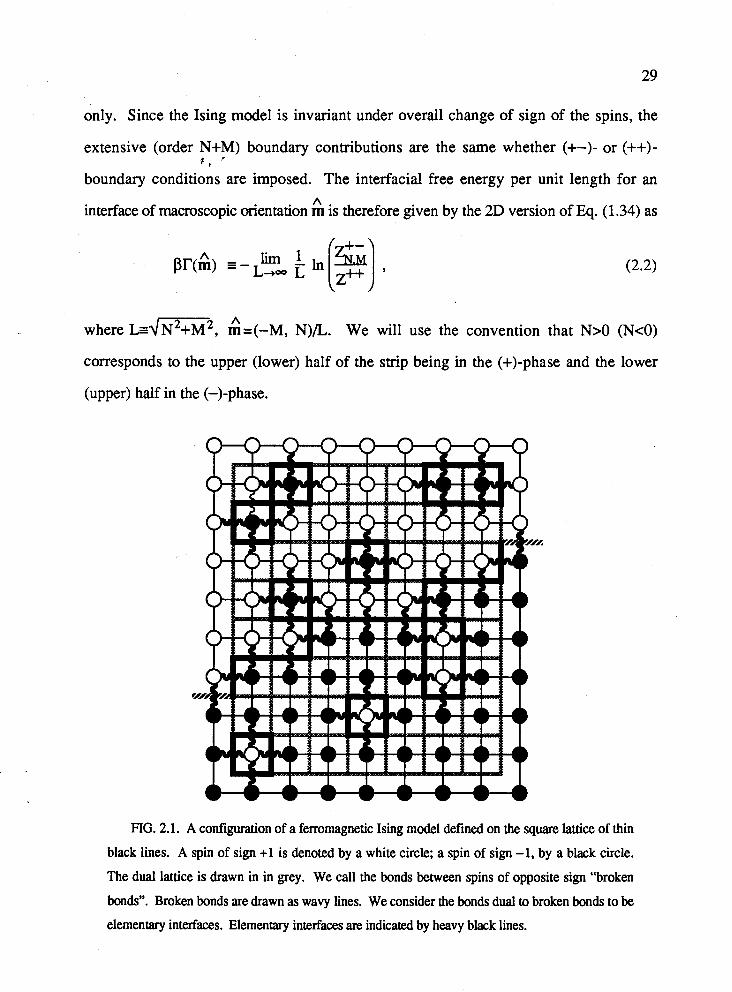
FIG. 2.1. A configuration of a ferromagnetic Ising model defined on the square lattice of thin

black lines. A spin of sign +1 is denoted by a white circle; a spin of sign -1, by a black circle.

The dual lattice is drawn in in grey. We call the bonds between spins of opposite sign "broken

bonds". Broken bonds are drawn as wavy lines. We consider the bonds dual to broken bonds to be

elementary interfaces. Elementary interfaces are indicated by heavy black lines.

A r (A) is related to the high-T correlation length of the dual system in the u

A direction, (*(u), via the well-known duality relation (e.g., Watson, 1968; Fisher, 1969;

P , ' Zia, 1978; Fradkin et al., 1978)

lirn 1. ~ ' ( k ) = - ~ + e a L ln (G*(~,~) d(N,M)) = l/(*(G),

A A where $(N,M)/L, with m u =O. Eq. (2.3) forms the basis of all solutions to the 2D ECS

problem which were known prior to our result Eq. (2.1): A calculation of the dual-lattice A

correlations (G*~,, in the thermodynamic limit, N,M+-, with m (u ) fixed,

A gives y(m), from which the ECS is determined via the Wulff construction.

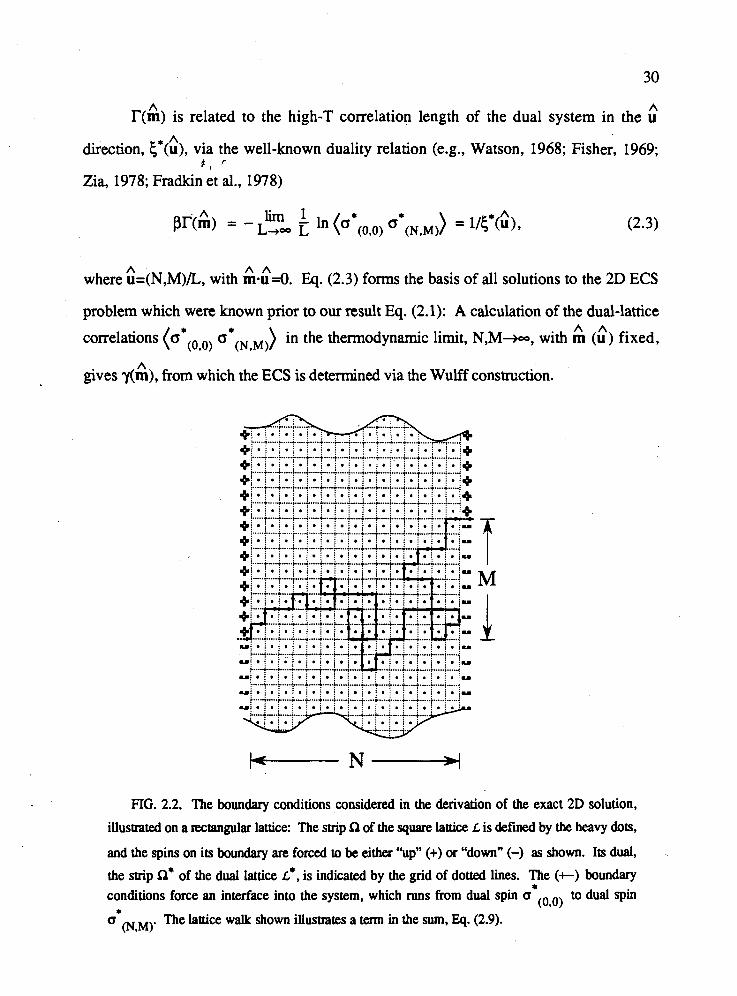
FIG. 2.2. The boundary conditions considered in the derivation of the exact 2D solution,

illustrated on a rectangular lattice: The strip R of the sqm lattice L is defined by the heavy dots,

and the spins on its boundary are forced to be either "up" (+) or "down" (-) as shown. Its dual,

the strip R* of the dual lattice L*, is indicated by the grid of dotted lines. The (t) boundary conditions force an interface into the system, which runs from dual spin to dud spin

* Q (NM)' The lattice walk shown illustrates a term in the sum, Eq. (2.9).

Here we shall calculate the ECS directly in the grand canonical ensemble, without A

going first through the auxiliary function T(m). If the ECS is represented in 2D Cartesian P , '

coordinates as Y(X), Eq. (1.38) becomes, in the variables of the present problem,

where the sum in the exponential extends over all microscopic interfaces whose segment A

lengths and normals are denoted by di and mi . In Eq. (2.4) the sum over M sums over an

ensemble of systems of all possible macroscopic interface orientations. We take each

system of this ensemble to be defined on i2 with t boundary conditions labeled by M. A

Because X is constant, Ci midi vanishes for microscopic interfaces forming closed loops.

Thus, the only contributions to the field term in the exponent arise from the line from (0,O)

to (N,M), and that contribution is -AX%c i Aidi = hXM, independent of the particular

path traced out by the line. [This simplification is a manifestation sf the fact that in two

dimensions there is no distinction between the ensembles Eq. (1.36) and Eq. (1.38).]

Thus, Eq. (2.5) becomes

We now evaluate Z&/zHusing the Vdovichenko-Feynrnan "random walker" method.

To see what the interface has to do with "walkers", consider the standard low-T

expansions of <i and (Kramers and Wannier, 1941):

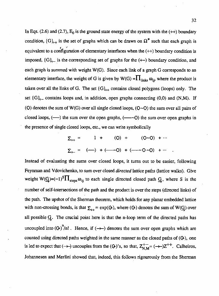
In Eqs. (2.6) and (2.7), Eo is the ground state energy of the system with the (tt) boundary

condition, (GZ, is the set of graphs which can be drawn on Q* such that each graph is $ '

equivalent to a configuration of elementary interfaces when the (+t) boundary condition is

imposed, ( G L is the corresponding set of graphs for the (t) boundary condition, and

each graph is summed with weight W(G). Since each link of a graph G corresponds to an

elementary interface, the weight of G is given by W(G) =HI& uij, where the product is

taken over all the links of G. The set {GZ, contains closed polygons (loops) only. The

set { G L contains loops and, in addition, open graphs connecting (0,O) and (N,M). If

(0) denotes the sum of W(G) over all single closed loops, ( 0 -0) the sum over all pairs of

closed loops, (-) the sum over the open graphs, (--0) the sum over open graphs in

the presence of single closed loops, etc., we can write symbolically

Instead of evaluating the sums over closed loops, it turns out to be easier, following

Feynman and Vdovichenko, to sum over closed directed lattice paths (lattice walks). Give

weight to each single directed closed path 9, where S is the

number of self-intersections of the path and the product is over the steps (directed links) of

the path. The upshot of the Sherman theorem, which holds for any planar embedded lattice

with non-crossing bonds, is that z,+ = exp(G), when ( 0 ) denotes the sum of W(5) over

all possible 9. The crucial point here is that the n-loop term of the directed paths has

uncoupled into ( ~ ) ~ / n ! . Hence, if (t) denotes the sum over open graphs which are

counted using directed paths weighted in the same manner as the closed paths of (G), one

is led to expect that (+) uncouples from the (O)'s, so that, q,~= (+)zH. Calheiros,

Johannesen and Merlini showed that, indeed, this follows rigourously from the Sherman

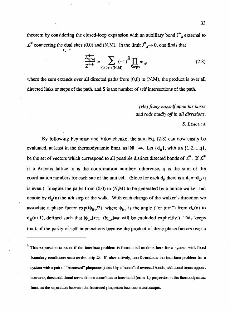
theorem by considering the closed-loop expansion with an auxiliary bond J*, external to

L* connecting the dual sites (0,O) and (N,M). In the limit J*,+ 0, one finds thatt r r '

where the sum extends over all directed paths from (0,O) to (N,M), the product is over all

directed links or steps of the path, and S is the number of self intersections of the path.

[He] jlung himself upon his horse and rode madly 08 in all directions.

By following Feynman and Vdovichenko, the sum Eq. (2.8) can now easily be

evaluated, at least in the thermodynamic limit, as INl+-. Let {dp}, with p . ~ {1,2, ...,q},

be the set of vectors which correspond to all possible distinct directed bonds of L*. If L*

is a Bravais lattice, q is the coordination number; otherwise, q is the sum of the

coordination numbers for each site of the unit cell. (Since for each dp there is a dv=-dp, q

is even.) Imagine the paths from (0,O) to (N,M) to be generated by a lattice walker and

denote by dp(n) the nth step of the walk. With each change of the walker's direction we

associate a phase factor e~p(i$~,/2), where $pv is the angle ("of turn") from dv(n) to

d,(n+l), defined such that I$pvl<a. (I$pvl=x will be excluded explicitly.) This keeps

track of the parity of self-intersections because the product of these phase factors over a

This expression is exact if the interface problem is formulated as done here for a system with fixed

boundary conditions such as the strip Q. If, alternatively, one formulates the interface problem for a

system with a pair of "frustrated" plaquettes joined by a "seam" of reversed bonds, additional terms appear;

however, these additional terms do not contribute to interfacial (order L) properties in the thermodynamic

limit, as the separation between the frustrated plaquettes becomes macroscopic.

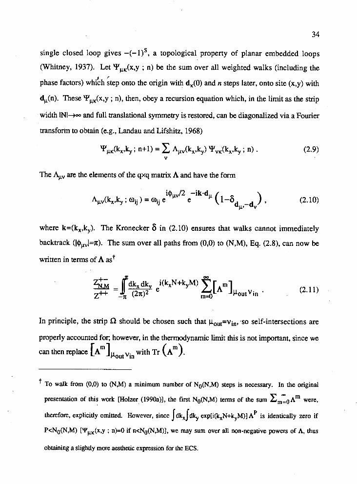
single closed loop gives -(-I)', a topological property of planar embedded loops

(Whitney, 1937). Let YpK(x,y ; n) be the sum over all weighted walks (including the

phase factors) whkh 'hep onto the origin with dK(0) and n steps later, onto site (x,y) with

dp(n). These YkK(x,y ; n), then, obey a recursion equation which, in the limit as the strip

width 1NI-w and full translational symmetry is restored, can be diagonalized via a Fourier

transform to obtain (e.g., Landau and Lifshitz, 1968)

The %v are the elements of the qxq matrix A and have the form

where k=(kx,ky). The Kronecker 6 in (2.10) ensures that walks cannot immediately

backtrack (I$pvl=x). The sum over all paths from (0,O) to (N,M), Eq. (2.8), can now be

In principle, the strip i2 should be chosen such that pOut=vin, .so self-intersections are

properly accounted for; however, in the thermodynamic limit this is not important, since we

can then replace [ A ~ ] pout vin with Tr ( 1 ~ ~ ) .

To walk from (0,O) to (N,M) a minimum number of NO(N,M) steps is necessary. In the original

presentation of this work Wolzer (1990a)], the first No(N,M) terms of the sum C,o~m were,

therefore, explicitly omitted. However, since jdkXjd4, exp[i(LxN+kyM)] A' is identically zero if

PcNO(N,M) [YpK(x,y ; n)=O if ncNO(N,M)I, we may sum over all non-negative powers of A, thus

obtaining a slightly more aesthetic expression for the ECS.

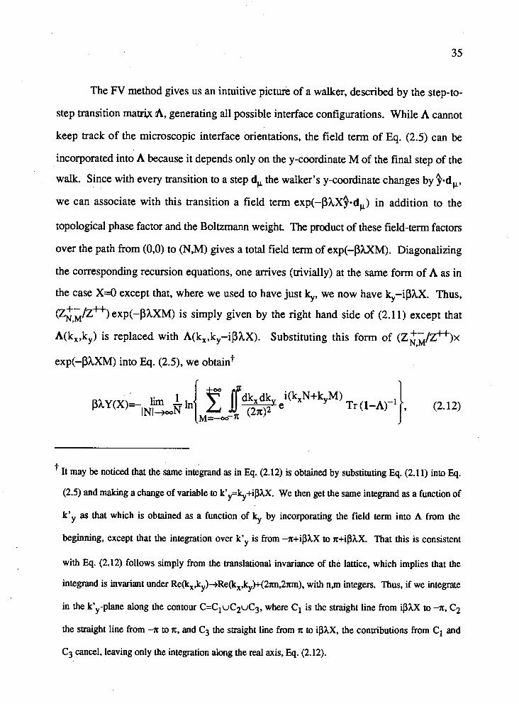
The FV method gives us an intuitive picture of a walker, described by the step-to-

step transition ma* A, generating all possible interface configurations. While A cannot

keep track of the microscopic interface orientations, the field term of Eq. (2.5) can be

incorporated into A because it depends only on the y-coordinate M of the final step of the

walk. Since with every transition to a step d, the walker's y-coordinate changes by Podc,

we can associate with this transition a field term e x p ( - ~ h ~ ~ - d p ) in addition to the

topological phase factor and the Boltzmann weight. The product of these field-term factors

over the path from (0,O) to (N,M) gives a total field term of exp(-PhXM). Diagonalizing

the corresponding recursion equations, one arrives (trivially) at the same form of A as in

the case X-0 except that, where we used to have just k,,, we now have V i P h X . Thus,

(<,;/zU) exp(-PhXM) is simply given by the right hand side of (2.1 1) except that

A(kx,ky) is replaced with A(kx,ky-iphX). Substituting this form of (~&/z+f)x

exp(-PhXM) into Eq. (2.5), we obtaint

It may be noticed that the same int&rand as in Eq. (2.12) is obtained by substituting Eq. (2.1 1) into Eq.

(2.5) and making a change of variable to k'y=%+iphX. We then get the same integrand as a function of

k'y as that which is obtained as a function of % by incorporating the field term into A from the

beginning, except that the integration over k'y is from -x+i$hX to x+iPhX. That this is consistent

with Eq. (2.12) follows simply from the translational invariance of the lattice, which implies that the

integrand is invariant under Re(k,,ky)+Re(kx,ky)t(2m,2xm), with n,m integers. Thus, if we integrate

in the k'y-plane along the contour C=C1uC2uC3, where C1 is the straight line from iPhX to -x, C2

the straight line from -x to A, and C3 the straight line from x to iphX, the contributions from C1 and

C3 cancel, leaving only the integration along the real axis, Eq. (2.12).

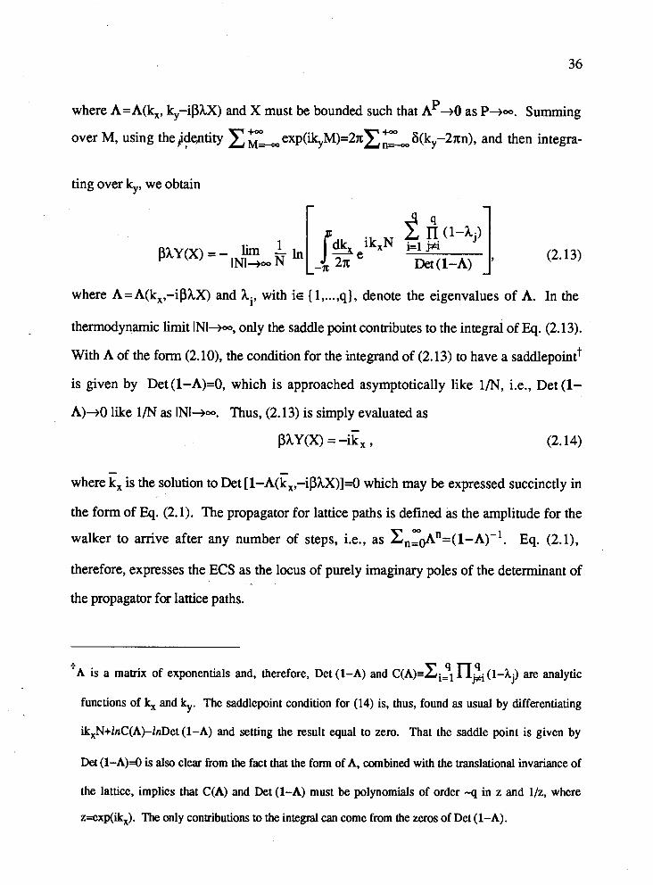
where A=A(kx, V i p h X ) and X must be bounded such that A'+O as P+-. Summing

over M, using the identity ~~-e~~(ik~~)=27t~~_"~6(k~-2n:n), - and then integra-

ting over ky, we obtain

where A=A(kx,-iphX) and hi, with i~ (1, ...,q), denote the eigenvalues of A. In the

thermodynamic limit INIj-, only the saddle point contributes to the integral of Eq. (2.13).

With A of the form (2. lo), the condition for the integrand of (2.13) to have a saddlePointi

is given by Det (1-A)=O, which is approached asymptotically like 1/N, i.e., Det (l-

A)+O like 1/N as INIj-. Thus, (2.13) is simply evaluated as -

phY(X) = -ikx ,

where is the solution to Det [I-A&,-~P;uL)]=o which may be expressed succinctly in

the form of Eq. (2.1). The propagator for lattice paths is defined as the amplitude for the

walker to arrive after any number of steps, i.e., as &,r&n=(l-~)-l. Eq. (2.1),

therefore, expresses the ECS as the locus of purely imaginary poles of the determinant of

the propagator for lattice paths.

9 t~ is s matrix of exponentials and, therefore. Det (1-A) and c ( A ) = ~ ~ . ~ n;i (14,) are analytic

functions of kx and ky. The saddlepoint condition for (14) is, thus, found as usual by differentiating

ikxN+lnC(A jlnDet ( 1 - and setting the result equal to zero. That the saddle point is given by

Det (1-A)=O is also clear Erom the fact that the form of A, combined with the translational invariance of

the lattice, implies that C(A) and Det (1-A) must be polynomials of order -q in z and llz, where

z=exp(ikx). The only contributions to the integral can come from the zeros of Det (1-A).

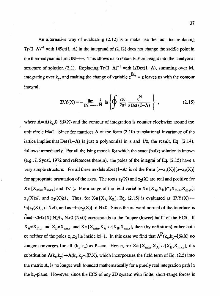
An alternative way of evaluating (2.12) is to make use the fact that replacing

Tr (1-A)-' with lDet(1-A) in the integrand of (2.12) does not change the saddle point in

the thermodynamic limit 1NI-w. This allows us to obtain further insight into the analytical

structure of solution (2.1). Replacing ~r (1-A)-' with l/Det(l-A), summing over M,

integrating over k,,, and making the change of variable eikx = z leaves us with the contour

integral,

1 PhY(X) = - lim - ln INl+- N

where A=A(kx,O-iphX) and the contour of integration is counter clockwise around the

unit circle 1z1=1. Since for matrices A of the form (2.10) translational invariance of the

lattice implies that Det (1-A) is just a polynomial in z and llz, the result, Eq. (2.14),

follows immediately. For all the Ising models for which the exact (bulk) solution is known

(e.g., I. Syozi, 1972 and references therein), the poles of the integral of Eq. (2.15) have a

very simple structure: For all these models zDet (1-A) is of the form [z-zl(X)][z-z2(X)]

for appropriate orientation of the axes. The roots zl(X) and %(X) are real and positive for

XE [Xmin,Xmax] and TcT,. For a range of the field variable XE [XA,XB]~[Xmin,Xmax],

z l (X)a and z2(X)21. Thus, for XE [XA,XB], Eq. (2.15) is evaluated as PhY(X)=-

ln[zl(X)], if NM, and as -ln[q(X)], if NcO. Since the outward normal of the interface is A m=(-cM>(X),N)/L, N>O (N<O) corresponds to the "upper (lower) half' of the ECS. If

XA+Xmi, and XB#Xm,, and XE [Xmin,XA]u [XB ,Xmax], then (by definition) either both

P or neither of the poles zl,z2 lie inside 1z1=1. In this case we find that A (kx,k,,-i$hX) no

longer converges for all (kx,ky) as P+-. Hence, for XE [Xmh,XA]~[XB,Xmax], the

substitution A(kx.k,,)+A(kx,ky-iPW(), which incorporates the field term of Eq. (2.5) into

the matrix A, is no longer well founded mathematically for a purely real integration path in

the kx-plane. However, since the ECS of any 2D system with finite, short-range forces is

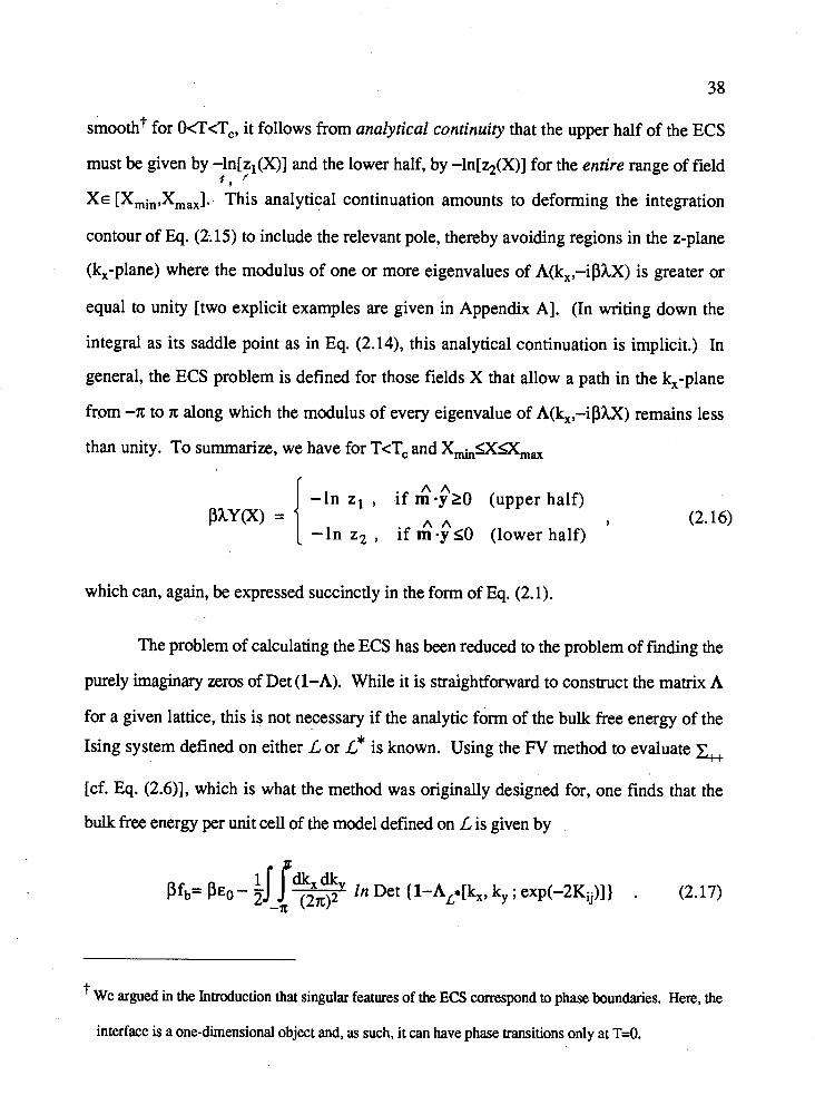
smootht for O(r(rC, it follows hom analytical continuity that the upper half of the ECS

must be given by -ln[zl(X)] and the lower half, by -ln[%(X)] for the entire range of field # r ,'

XE [Xmi,,XmaX]. This analytical continuation amounts to deforming the integration

contour of Eq. (2; 15) to include the relevant pole, thereby avoiding regions in the z-plane

(kx-plane) where the modulus of one or more eigenvalues of A(kx,-iphX) is greater or

equal to unity [two explicit examples are given in Appendix A]. (In writing down the

integral as its saddle point as in Eq. (2.14), this analytical continuation is implicit.) In

general, the ECS problem is defined for those fields X that allow a path in the kx-plane

from -a to a along which the modulus of every eigenvalue of A(k,,-iphX) remains less

than unity. To summarize, we have for T<Tc and X,,.,$XIX,, I

A A -In zl , if m *y 20 (upper half)

A A 9 - In z2 , if m *y 1 0 (lower half)

which can, again, Se expressed succinctly in the form of Eq. (2.1).

The problem of calculating the ECS has been reduced to the problem of finding the

purely imaginary zeros of Det (1-A). While it is straightforward to construct the matrix A

for a given lattice, this is not necessary if the analytic form of the bulk free energy of the

Ising system defined on either L or L* is known. Using the W method to evaluate &+

[cf. Eq. (2.6)], which is what the method was originally designed for, one finds that the

bulk free energy per unit cell of the model defined on L is given by

'j JQX in Det (1-Al[kx, ky ; exp(-Xi,)] ) . (2.17) pfb= ~ E O - 3 (2,+ -II;

We argued in the Intmduction that singular features of the ECS correspond a phase boundaries. He=, the

interface is a one-dimensional object and, as such, it can have phase transitions only at T=O.

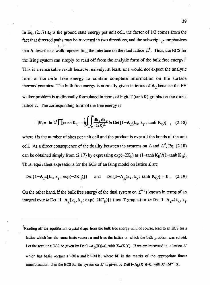
In Eq. (2.17) q, is the ground state energy per unit cell, the factor of 112 comes from the

fact that directed paths may be traversed in two directions, and the subscript L* emphasizes 2 , '

that A describes a walk representing the interface on the dual lattice L*. Thus, the ECS for

the Ising system can simply be read off from the analytic form of the bulk free energy!?

This is a remarkable result because, naively, at least, one would not expect the analytic

form of the bulk free energy to contain complete information on the surface

thermodynamics. The bulk free energy is normally given in terms of ALbecause the FV

walker problem is traditionally formulated in terms of high-T (tanh K) graphs on the direct

lattice L The corresponding form of the free energy is

where Cis the number of sites per unit cell and the product is over all the bonds of the unit

cell. As a direct consequence of the duality between the systems on L and L*, Eq. (2.18)

can be obtained simply from (2.17) by expressing exp(-2Kij) as (1-tanh Kij)/(l+tanh Kij) . Thus, equivalent expressions for the ECS of an Ising model on lattice L are

Da { 1-AL*[kx, ky ; exp(-2Kij)] } and Det [1-AL(kx, k,, ; tanh &,)I = 0 . (2.19)

On the other hand, if the bulk free energy of the dual system on L* is known in terms of an

integral over l n D a (1-AJk,, ky ; e~p(-2K*~,)]} (low-T graphs) or in Det [1-AL*(kx, ky

' ~ e a d i n ~ off the equilibrium crystal shape from the bulk free energy will, of course, lead to an ECS for a

lattice which has the same basis vectors a and b as the lattice on which the bulk problem was solved.

Let the resulting ECS be given by Det[l-Ab(X)]=O, with X=(X,Y). If we are interested in a lattice L'

which has basis vectors a'=M a and b'=M b, where M is the matrix of the appropriate linear

transformation, then the ECS for the system on L' is given by ~et[l-A~(X')]=O, with x'=M-1 X.

; tanh K*ij)] (high-T graphs), the expressions (2.19) [and, of course, also (2.17) and

(2.18)] may be obtained via the duality transformation e~p(-2K*~~) -t tanh qj. f f '

Once one has obtained the ECS from Eq. (2.1), one can use the inverse of the

Wulff construction to determine the corresponding interfacial free energy per unit length

r(e), or equivalently, the inverse of the (anisotropic) high-T correlation length 5*(8+.n/2)

of the dual system [cf. Eq. (2.3)]. Once the ECS is known in the form Y(X), the (2D)

analytical form of the inverse Wulff construction is given by

a Y r(8)=1/5*(0+1~/2) = hX sine +hY cose ; tan 0 - - ax . Eq. (2.20) is easily derived by expressing (1.12) in 2D polar coordinates and solving for

A A r(8) and aY/aX. With appropriate choice of basis vectors [a=x and b=y for the ECS's of

Table 2.1 (see also Fig. 2.5)], Eqs. (2.20) give two polynomials in cosh(phX) and

cosh(phY). Since these two polynomial generally combine to give a polynomial in a single

variable of order higher than 4th, it is generically not possible to obtain an analytic, closed

form expression for r(B). An exception is the rectangular lattice (see Appendix B). Of

course, Eq. (2.20) can always be implemented numerically to obtain r(8) to arbitrary

accuracy.

Figures 2.3 and 2.4 show two examples of ECS's and corresponding interfacial

free energies typical of ferromagnetic Ising models. These shapes display the following

universal features of 2D Ising ECS's (Zia, 1986): 1) The ECS becomes a circle as T+Tc-.

For less symmetric lattices the ECS becomes an ellipse as T+Tc- (see Fig. 2.10). This is

a result of the fact that the lattice anisotropy is a marginal variable (in the renormalization-

group sense). 2) The ECS, as obtained from Eq. (2.1) for fixed h, vanishes in all 2 2 directions linearly with t a (Tc-T) as t+O+, i.e., the R(B,T)=~= - tp with the surface

critical exponent p=l (and with a &dependent amplitude in the generic case of an

asymptotically elliptical ECS). That p=l follows immediately from the duality relation

(2.3) since the bulk correlation length 5 diverges like t-v and we know that v=l from the + f

exact bulk solution. p=l is consistent with the hyperscaling relation p=@-l)v (Widom,

1965). In Table 2.1 we give, for convenience of the reader, the analytical form for the ECS

of the Ising model defined on a number of commonly encountered lattices (Fig. 2.5). The

results for the ECS of the square, triangular, and honeycomb lattices have been obtained

previously via the canonical formulation [see Eq. (2.3)] from the known direction

dependent correlation lengths of these lattices (rectangular lattice: Cheng and Wu, 1967;

see also McCoy and Wu, 1973; triangular/honey comb lattice: Vaidya, 1976). We

obtained the equations for the Kagomk and "Union Jack" lattices and their duals by explicit

construction of the matrix A. For the special cases, K1=K4, K2=K3, and K5=K6 for the

Kagomk lattice and K1=K2=K3=K4 and K5=Ks for the "Union Jack" lattice, our result for

Det (1-A) reduces to that which can be read off from the bulk free energy as obtained by

Kano and Naya in 1953 and by Vaks et d. in 1866, respectively.

In the derivation above, we had ferromagnetic Ising models in mind. However, the

properties of the model crucial for our derivation are satisfied for a wider class of models.

Hurst and Green showed in 1960 (see also Hurst, 1966) that the FV method is equivalent

to the Pfaffian method, which can be used to solve any model which can be written as a

free fermion field theory, i.e., a field theory which is quadratic in fermionic operators. The

factors of (-1) which appear in the FV method are directly related to the (- 1)'s of fermion

anticommutators, and the uncoupling of directed graphs, necessary for the FV method to

work, is precisely due to the field theory being free. The upshot of this equivalence is that

we know the ECS for any model solvable by the Pfaffian or IT method in the form of the

poles of the determinant of the free-fermion propagator, Eq. (2.1), provided that the N

walk can be identified with an interface between coexisting phases.

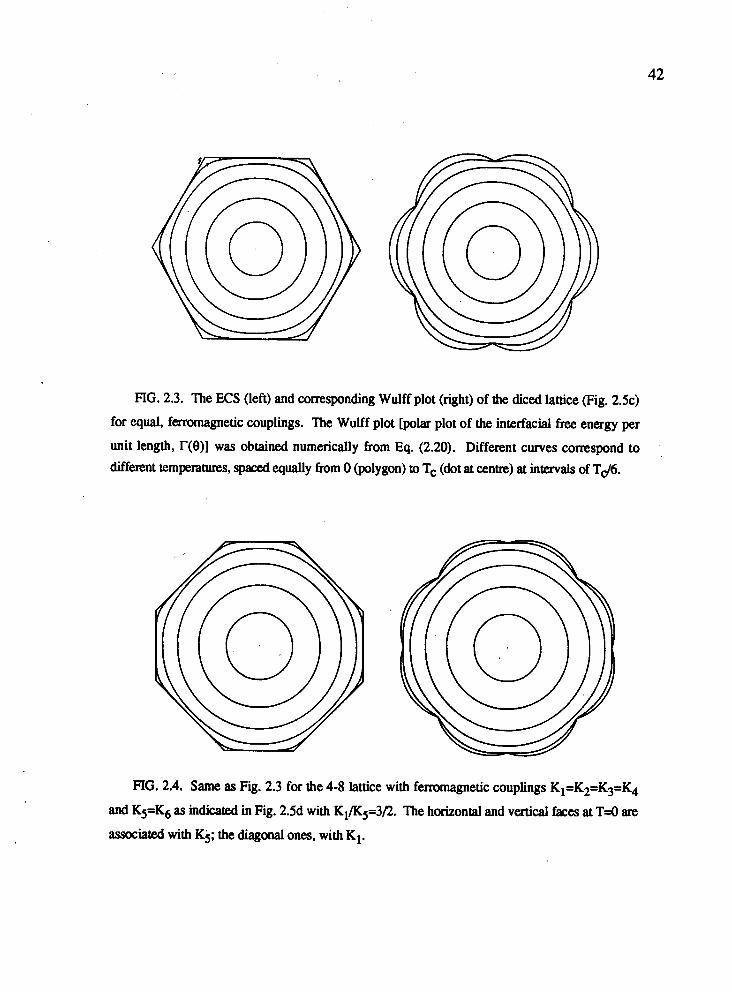
FIG. 2.3. The ECS (left) and corresponding Wulff plot (right) of the diced lattice (Fig. 2.5~)

for equal, ferromagnetic couplings. The Wulff plot [polar plot of the interfacial free energy per

unit length, r(0)] was obtained numerically from Eq. (2.20). Different curves correspond to

different temperatures, spaced equally from 0 (polygon) to Tc (dot at centre) at intervals of Td6.

FIG. 2.4. Same as Fig. 2.3 for the 4-8 lattice with ferromagnetic couplings Kl=K2=K3=K4

and K5=K6 as indicated in Fig. 2.5d with K1/Kg=3/2. The horizontal and vertical faces at T=O are

associated with Kj; the diagonal ones, with K1.

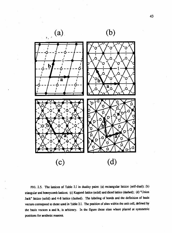
FIG. 2.5. The lattices of Table 2.1 in duality pairs: (a) rectangular lattice (self-dual); (b)

triangular and honeycomb lattices; (c) Kagom6 lattice (solid) and diced lattice (dashed); (d) "Union

Jackw lattice (solid) and 4-8 lattice (dashed). The labeling of bonds and the definition of basis

vectors correspond to those used in Table 2.1. The position of sites within the unit cell, defined by

the basis vectors a and b, is arbitrary. In the figure these sites where placed at symmetric

positions for aesthetic reasons.

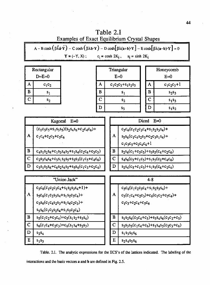
Table 2.1 Exam~les of Exact Eauilibrium Crystal Sha~es

Rectangular D=E=O

S2

"Union Jack" I

I Honeycomb I

Diced E=O

Table. 2.1. The analytic expressions for the ECS's of the lattices indicated. The labeling of the

interactions and the basis vectors a and b are defined in Fig. 2.5.

2.3 An example of non-Ising free-fermion crystal shapes: The modified KDP model.

4 ' ,-

We will now demonstrate the validity of Eq. (2.1) for the modified KDP model, a

non-Ising free-fermion model. To be precise, we shall show that the purely imaginary

poles of the determinant of the free-fermion propagator of the modified KDP model will

correctly give the ECS of the dual model. The dual model turns out to be the limit of an

antiferromagnetic Ising model on a triangular lattice as the interactions become infinite. The

resulting ECS's have sharp corners for any T<Tc. The interface configurations of this

model are extremely simple, so the solutions obtained from (2.1) can be confirmed via an

independent elementary calculation. Historically, the 3D KDP model was originally

proposed by Slater in 1941 as a model having the characteristics of the ferroelectric

potassium dihydrogen phosphate (KDP) KH2P04. The 2D version of the Slater KDP

model was solved by Lieb, and independently by Sutherland, in 1967. The modified KDP

model is a s p ~ i a l (more simple) version of the KDP model in which a certain configuration

has been suppressed but which still has many of the essential features of the full KDP

model (Lieb and Wu, 1972).

The modified KDP model is a special case of the eight-vertex model. The square-

lattice eight-vertex model is defined by eight types of vertices, as shown in Fig. 2.6, which

must be placed on the vertices of a square lattice, such that arrows from different vertices

sharing the same bond point in the same direction. Each vertex carries a Boltzmann weight

oi=exp(-pei), i=1,2,..,8. When these weights satisfy the so-called free-fermion

condition (Hurst and Green, 1960; Hurst, 1966; Lieb and Wu, 1972),

the square lattice eight-vertex model is solvable by the Pfaffian method and, therefore, by

the FV method.# Eg. (2.21) is satisfied by any eight-vertex model at one particular I

temperature. When the weights o i are chosen such that (2.21) is satisfied at all

temperatures, the model is known as the free-fermion model (Lieb and Wu, 1972).

Depending on the particular choices for the COi, the free-fermion model can be shown to be

either trivial (decoupled 1D chains), equivalent to the Ising model on a triangular lattice, or,

in a certain limiting case (see below), equivalent to the modified KDP model, which in turn

turns out to be equivalent to the close-packed dimer model on a hexagonal lattice (Wu,

FIG. 2.6. The eight vertex configurations of the eight-vertex model. As an alternative to

representing vertex configurations by arrows, one can represent them by "bond arrangements".

These bond arrangements are constructed from the arrow representation by first choosing

(arbitrarily) a vertex which corresponds to no bonds (no bold lines), the basis. Other bond

configurations are then constructed from the basis by drawing a bond for every arrow pointing in a

direction opposite to that of the corresponding arrow of the basis vertex. (a), (b), and (c) show

three of the eight possible bond arrangements based on the vertices 2,3, and 4, respectively.

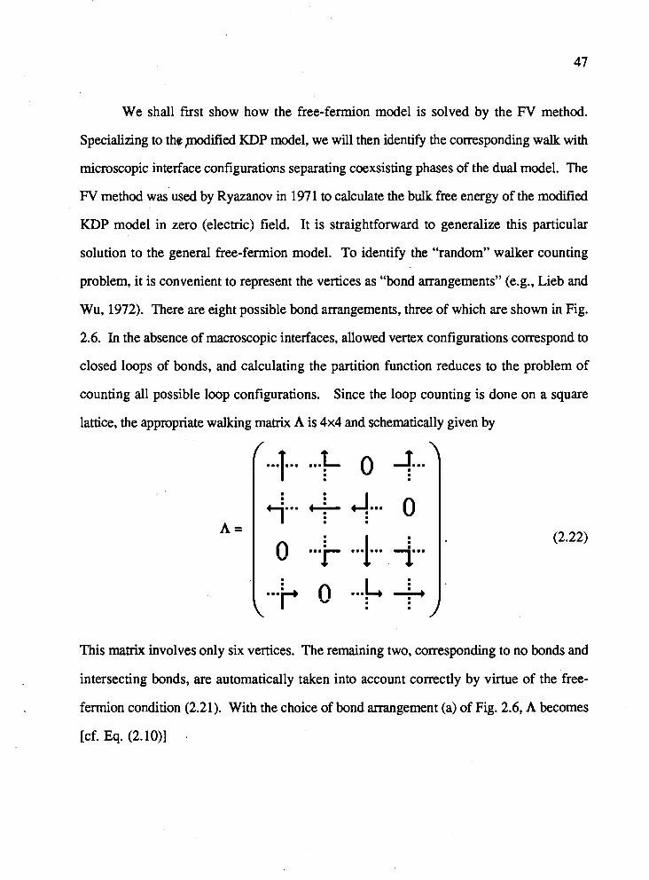
We shall first show how the free-fermion model is solved by the FV method.

Specializing to the podifid KDP model, we will then identify the corresponding walk with

microscopic interface configurations separating coexsisting phases of the dual model. The

FV method was used by Ryazanov in 197 1 to calculate the bulk free energy of the modified

KDP model in zero (electric) field. It is straightforward to generalize this particular

solution to the general free-fermion model. To identify the "random" walker counting

problem, it is convenient to represent the vertices as "bond arrangements" (e.g., Lieb and

Wu, 1972). There are eight possible bond arrangements, three of which are shown in Fig.

2.6. In the absence of macroscopic interfaces, allowed vertex configurations correspond to

closed loops of bonds, and calculating the partition function reduces to the problem of

counting all possible loop configurations. Since the loop counting is done on a square

lattice, the appropriate walking matrix A is 4x4 and schematically given by

This matrix involves only six vertices. The remaining two, corresponding to no bonds and

intersecting bonds, are automatically taken into account correctly by virtue of the free-

fermion condition (2.21). With the choice of bond arrangement (a) of Fig. 2.6, A becomes

[cf. Eq. (2. lo)] .

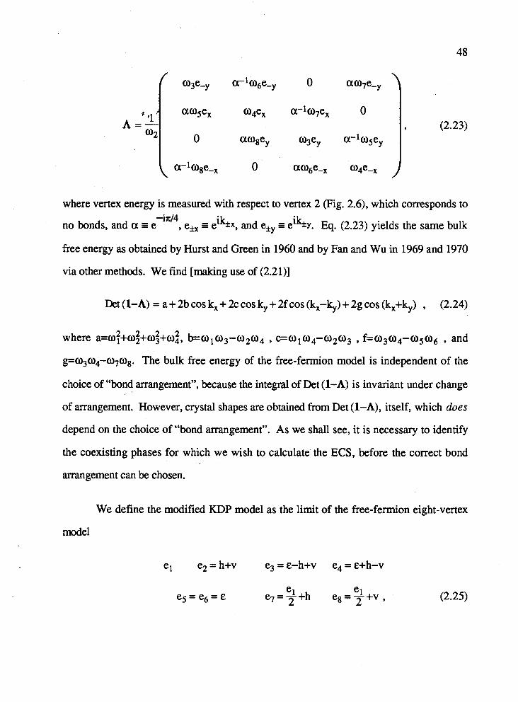
where vertex energy is measured with respect to vertex 2 (Fig. 2.6), which corresponds to -in14

no bonds, and a = e , e*, = - eikx, and eky = ei&y. Eq. (2.23) yields the same bulk

free energy as obtained by Hurst and Green in 1960 and by Fan and Wu in 1969 and 1970

via other methods. We find [making use of (2.21)]

Det (I-A) = a + 2b cos kx + 2c cos k, + 2f cos (k,-ky) + 2g cos (kx+ky) , (2.24)

where a = o ~ + a ~ + a ~ + w ~ , b=wl a3-a2a4 , c=ola4-a2a3 , a6 , and

The bulk free energy of the free-fermion model is independent of the

choice of "bond arrangement", because the integral of Det (1-A) is invariant under change

of arrangement. However, crystal shapes are obtained from Det (1-A), itself, which does

depend on the choice of "bond arrangement". As we shall see, it is necessary to identify

the coexisting phases for which we wish to calculate' the ECS, before the correct bond

arrangement can be chosen.

We define the modified KDP model as the limit of the free-fermion eight-vertex

model

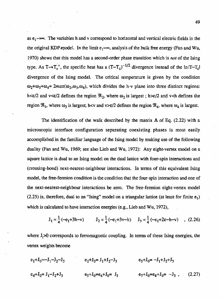
as el+-. The variables h and v correspond to horizontal and vertical electric fields in the

the original KDPqodel. In the limit el=-, analysis of the bulk free energy (Fan and Wu,

1970) shows that this model has a second-order phase transition which is not of the Ising

type. As T + T ~ , the specific heat has a (T-T,)-lR divergence instead of the 1nlT-TcI

divergence of the Ising model. The critical temperature is given by the condition

CII~+CO~+CO~= 2max(a2,a3,a4), which divides the h-v plane into three distinct regions:

he12 and vc~12 defines the region 912, where a2 is largest ; h x l 2 and vch defines the

region 913, where 03 is largest; hcv and v>d2 defines the region 914, where is largest.

The identification of the walk described by the matrix A of Eq. (2.22) with a

microscopic interface configuration separating coexisting phases is most easily

accomplished in the familiar language of the Ising model by making use of the following

duality (Fan and Wu, 1969; see also Lieb and Wu, 1972): Any eight-vertex .model on a

square lattice is dual to an Ising model on the dual lattice with four-spin interactions and

(crossing-bond) next-nearest-neighbour interactions. In terms of this equivalent Ising

model, the free-fermion condition is the condition that the four-spin interaction and one of

the next-nearest-neighbour interactions be zero. The free-fermion eight-vertex model

(2.25) is, therefore, dual to an "Ising" model on a triangular lattice (at least for finite el)

which is calculated to have interaction energies (e.g., Lieb and Wu, 1972),

where Ji>O corresponds to ferromagnetic coupling. In terms of these Ising energies, the

vertex weights become

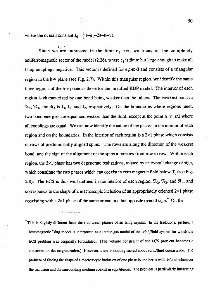
1 where the overall constant Jo = 4 (-el-2~-h-v).

P f ' Since we are interested in the limit el+-, we focus on the completely

antiferromagnetic sector of the model (2.26), where el is finite but large enough to make all

Ising couplings negative. This sector is defined for el>&* and consists of a triangular

region in the h-v plane (see Fig. 2.7). Within this triangular region, we identify the same

three regions of the h-v plane as those for the modified KDP model. The interior of each

region is characterized by one bond being weaker than the others. The weakest bond in

s 2 , 313, and s4 is J3, J1, and J2, respectively. On the boundaries where regions meet,

two bond energies are equal and weaker than the third, except at the point h=v=E/2 where

all couplings are equal. We can now identify the nature of the phases in the interior of each

region and on the boundaries. In the interior of each region is a 2x1 phase which consists

of rows of predominantly aligned spins. The rows are along the direction of the weakest

bnd , and the sign of the alignment of the spins alternates from row to row. Within each

region, the 2x1 phase has two degenerate realizations, related by an overall change of sign,

which constitute the two phases which can coexist in zero magnetic field below T, (see Fig.

2.8). The ECS is thus well defined in the interior of each region, 9?2, s 3 , and s 4 , and

corresponds to the shape of a macroscopic inclusion of an appropriately oriented 2x1 phase

coexisting with a 2x1 phase of the same orientation but opposite overall sign! On the

'This is slightly different from the traditional picture of an Ising crystal. In the traditional picture, a

ferromagnetic Ising model is interpreted as a lattice-gas model of the solid/fluid system for which the

ECS problem was originally formulated. (The volume constraint of the ECS problem becomes a

constraint on the magnetization.) However, there is nothing sacred about solid/fluid coexistence. The

problem of finding the shape of a macroscopic inclusion of one phase in another is well defined whenever

the inclusion and the surrounding medium coexist in equilibrium. The problem is particularly interesting

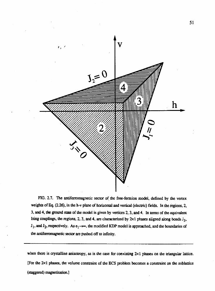
FIG. 2.7. The antifemmagnetic sector of the free-fermion model, defined by the vertex

weights of Eq. (2.26). in the h-v plane of horizontal and vertical (electric) fields. In the regions, 2,

3, and 4, the gmund state of the model is given by vertices 2,3, and 4. In terms of the equivalent

Ising couplings, the regions, 2,3, and 4, are characterized by 2x1 phases aligned along bonds J3,

J1, and J2, respectively. As el+, the modified KDP model is approached, and the boundaries of

the antiferromagnetic sector are pushed off to infmity.

when there is crystalline anisotropy, as is the case for coexisting 2x1 phases on the triangular lattice.

[For the 2x1 phases, the volume constraint of the ECS problem becomes a constraint on the sublattice

(staggered) magnetization.]

boundaries where regions meet, the ground state is macroscopically degenerate and there is

no ordered phase &tf af~y temperature.

The walk of the FV method can now easily be identified as a microscopic interface

configuration: The bold lines of bond arrangements correspond to composite elementary

interfaces on the hexagonal lattice dual to the triangular Ising system (2.26), as shown in

Fig. 2.9. Depending on which bond arrangement is chosen, these interface configurations

carry different vertex weights ei [Fig. 2.61. To interpret these energies as the energies

needed to create the composite interfaces of Fig. 2.9 from the ground state configuration,

we must first identify the ground-state energy per vertex. It follows from Eqs. (2.27) that

the energy for the the 2x1 ground state of s 2 , s 3 , and s4 corresponds to the energy of

vertex 2,3, and 4, respectively. Subtracting the ground state energies, one can now easily

identify the vertex energies of bond arrangements (a), (b), and (c) as precisely the energies

needed to create the correspondixg broker, bonds per vertex from the 2x1-phase ground

states of regions s 2 , s 3 , and s 4 , respectively (see Fig's 2.6 and 2.9). Different bond

arrangements result in different weights for the entries of the matrix A [cf. Eq. (2.22)],

which leads to different functions Det (1-A). It is now clear that the matrix A based on

bond arrangement (a), with vertex 2 describing the ground state;can describe elementary

interfaces of the antiferromagnetic triangular Ising model only in s2. To obtain the ECS in

s3 and s 4 , A must be based on bond arrangements (b) and (c), respectively. Det (1-A)

for s3 is obtained from Eq. (2.24) by making the substitutions (b,f,g)+(-b,-f,-g), and

for s 4 , by making the substitutions (c,f,g)+(-c,-f,-g).

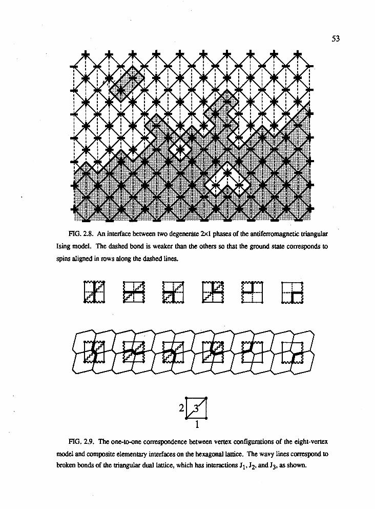
FIG. 2.8. An interface between two degenerate 2x1 phases of the antiferromagnetic triangular

Ising model. The dashed bond is weaker than the others so that the ground state corresponds to

spins aligned in mws along the dashed lines.

FIG. 2.9. The one-to-one correspondence between vertex configurations of the eight-vertex

model and composite elementary interfaces on the hexagonal lattice. The wavy lines correspond to

broken bonds of the triangular dual lattice, which has interactions J1, J2, and J3, as shown.

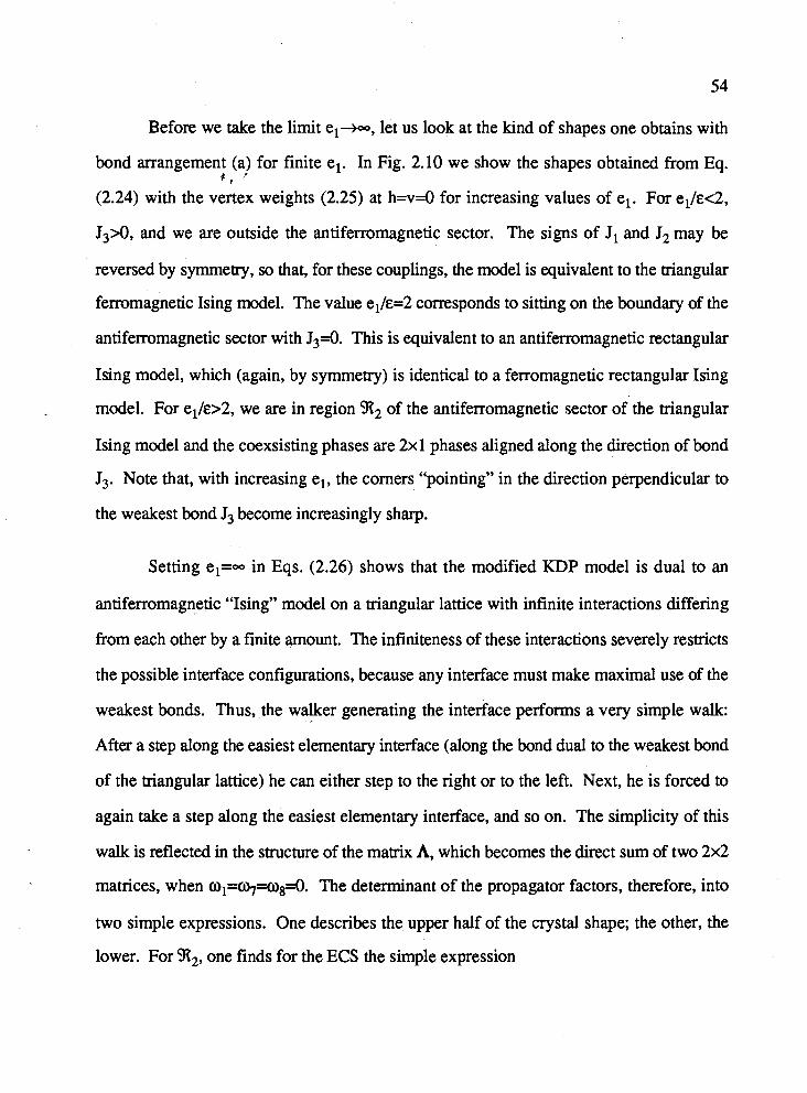
Before we take the limit el+-, let US look at the kind of shapes one obtains with

bond arrangement (a) for finite el. In Fig. 2.10 we show the shapes obtained Erom Eq. P f '

(2.24) with the vertex weights (2.25) at h=v=O for increasing values of el. For el/&c2,

J3>0, and we are outside the antiferromagnetic sector. The signs of J1 and J2 may be

reversed by symmetry, so that, for these couplings, the model is equivalent to the triangular

ferromagnetic Ising model. The value el/&=2 corresponds to sitting on the boundary of the

antiferromagnetic sector with J3=0. This is equivalent to an antiferromagnetic rectangular

Ising model, which (again, by symmetry) is identical to a ferromagnetic rectangular Ising

model. Far el/&>2, we are in region 912 of the antiferromagnetic sector of the triangular

Ising model and the coexsisting phases are 2x1 phases aligned along the direction of bond

J3. Note that, with increasing el, the comers "pointing" in the direction perpendicular to

the weakest bond J3 become increasingly sharp.

Setting el=- in Eqs. (2.26) shows that the modified KDP model is dual to an

antiferromagnetic "Ising" model on a triangular lattice with infinite interactions differing

from each other by a finite amount. The infiniteness of these interactions severely restricts

the possible interface configurations, because any interface must make maximal use of the

weakest bonds. Thus, the walker generating the interface performs a very simple walk:

After a step along the easiest elementary interface (along the bond dual to the weakest bond

of the triangular lattice) he can either step to the right or to the left. Next, he is forced to

again take a step along the easiest elementary interface, and so on. The simplicity of this

walk is reflected in the structure of the matrix A, which becomes the direct sum of two 2x2

matrices, when 01=~=08=0. The determinant of the propagator factors, therefore, into

two simple expressions. One describes the upper half of the crystal shape; the other, the

lower. For 912, one finds for the ECS the simple expression

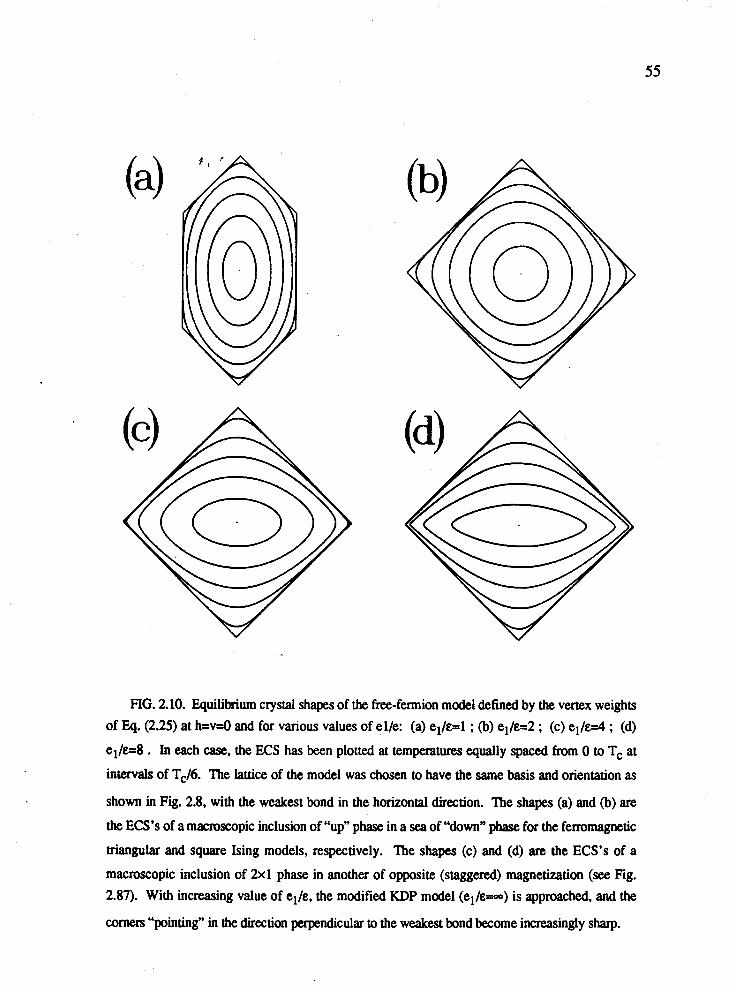
FIG. 2.10. Equilibrium crystal shapes of the free-fermion model defined by the vertex weights

of Eq. (2.25) at h=v=O and for various values of elle: (a) el/&=l ; (b) el/&=2 ; (c) el/&=4 ; (d)

el/&=8 . In each case, the ECS has been plotted at temperatures equally spaced from 0 to Tc at

intervals of Tc/6. The lattice of the model was chosen to have the same basis and orientation as

shown in Fig. 2.8, with the weakest bond in the horizontal direction. The shapes (a) and (b) are

the ECS's of a m~cmscopic inclusion of "up" phase in a sea of "downn phase for the ferromagnetic

triangular and square Ising models, respectively. The shapes (c) and (d) are the ECS's of a

macroscopic inclusion of 2x1 phase in another of opposite (staggered) magnetization (see Fig.

2.87). With increasing value of el/&, the modified KDP model (el/e=-) is approached, and the

corners "pointing" in the direction perpendicular to the weakest bond become increasingly sharp.

o3 e-Pxx + o4 e -PXY - o2 = 0 and (X,Y)+(-X,-Y) , (~ ,v )E 312 . (2.28)

The corresponding equations for S3 and s4 are obtained from Eq. (2.28) by making the

substitutions a4+ -614 and a3+ -03, respectively. Notice that the pair of functions

(2.28), (and the corresponding ones in 913 and S4 ) describe curves of infinite extent and

that the ECS is to be interpreted as the convex region enclosed by the two functions for

TOc. Where the pair of curves intersect, the ECS has a sharp comer which moves toward

the origin like (T-T)'~, as T+TJ. In all other directions the ECS vanishes linearly with

T, as T+Tc-. The sharp corners and the fact that the crystal shape appears to be

analytically continued beyond the convex regiont are unusual features of the ECS and are a

direct result of the infiniteness of the interactions. To gain further insight into the physical

origin of these features, we make use of the simplicity of the interface configurations to

calculate - in a very direct and elementary manner - the interfacial free energy and the crystal

shape.

Consider the infinite-interaction "Ising" model dual to the KDP model on an

arbitrary triangular lattice, so that the corresponding FV walk takes place on an arbitrary

hexagonal lattice. Let the easiest steps on the hexagonal lattice be denoted by d, and 4,

and denote the steps to the right and left of d, by 4 and dpespectively. Because of the

In the antiferromagnetic sector, there are real, unbounded solutions Y(X) to Det[l-A(X,Y)]=O for

XE [-m,X&[XR,~] even for finite el. We believe that these solutions have no physical significance,

at least not in the context of ECS's. The expression for Y(X) in terms of a sum over A's [cf. Eq. (2.12)l

becomes formally divergent for XE [--,XL]u[xR,-]. When el=-, XL and X, coincide with the

"boundaries" Xmi, and X,,, of the ECS. (For purely ferromagnetic king models, no such real,

unbounded solutions exist.)

infiniteness of the interactions, the walker actually perfoms a walk on a rectangular lattice

with the composite steps f dl and +d2, where dl=dw+d, and d2=d,+dc. Since a step +dl 2 , *

or f d 2 of given sign must be followed by a step of the same sign, the only interfaces

available to the (say) upper half of the ECS must have tangent vectors which lie between dl

and d2 (see Fig. 2.1 1). It is precisely the absence of other interface orientations which

causes the sharp corners of the ECS. The zero-temperature character of the infinite

interactions manifests itself in the fact that the entropy of a walk from the origin to the point

R = ndl+ m d2, (m,n > 0) is simply given by the zero-temperature entropy,

In [(n+m)! / (n! m!)], at all temperatures. If El and E2 denote the costs in energy of

taking steps f dl and +d2, we can immediately write down the corresponding free energy

per unit length, QB), as

A where fi a n/R, 6 =- m/R, 8 is measured clockwise from the zxd2 direction, and

cos em,,= dl*d2/(dld2). For other directions, r (8 ) is infinite. Explicitly, we find - m = (cose - s ine cot emax)/d2 and fi = sin W(dl sine,,,). Performing the Wulff

construction for each of the two branches of r (8 ) separately (i.e., separately for

0~ [O,e,,] and for 0~ [X,X+~,,,] ), one finds that the envelope of the Wulff lines for

each branch produces an infinitely extended curve. The pair of curves thus obtained is

given by

B[E1+~2+(d1+d2):y1 = 2 cosh ( $ E ~ - E ~ + ( ~ ~ - ~ ~ ) * Y ] ) and (dl ,d2)+(-dl ,-d2), (2.30) ' e2

FIG. 2.1 1. The Feynman-Vdovichenko walker for the modified KDP model performs a very

simple walk on the honeycomb lattice: The infiniteness of the interactions forces the walker to

make maximal use of the lowest-energy step, which we take to be kd,. Every step d, is followed

by a step d, or db which must be followed again by a step d,, and so on. Thus, the walk takes

place effectively on a square lattice with the composite steps *dl and id2. Since every composite

step must be followed by a composite step of the same sign, only the shaded regions are accessible

to a walker starting out at a given lattice site. The fact that directions outside the shaded regions

are forbidden is what causes the sharp comers of the ECS of the modified KDP model and gaps in

the corresponding Wuiff plot.

where Ys(-Y,X). Eqs. (2.28) and the corresponding equations in S3 and S4 are special A h A A A A A h

cases of (2.30) corresponding to (dl,dz) equal to (-y,x), (x ,x+y), and (x+y,y), I , '

respectively, and are just rotations and linear distortions of one another. The interior

envelope of all Wulff planes is just the convex region enclosed by both curves and results

in a ECS with sharp corners (see Fig. 2.12):

FIG. 2.12. The ECS of the modified KDP model (solid lines, left) and the corresponding

Wulff plot (right) for h=v=O. The curves have been plotted at temperatures equally spaced from 0 to Tc at intervals of Tc/5. The dual lattice for the model has been chosen to have the basis and

orientation shown in Fig. 2.8. At finite T, those orientations conesponding to the dashed lines do

not contribute to the ECS and are, therefore, thermodynamically unstable.

For those orientations 8 for which the function T(8) defined in Eq. (2.29) does not contribute to the ECS,

r(8) is not an interfacial free energy. If R=(n,m) is not tangent to the ECS, an interface from (0,O) to

(n.m) will consist of two macroscopically linear segments in accordance with the lever rule [e.g., M.

Wortis (1988)l. The single sharp corner thus generated (costing infinite energy but having zero

thermodynamic weight) is strictly disallowed in the calculation leading to (2.29). Thus, only for

orientations tangent to the ECS does (2.29) have meaning as the interfacial free energy of the modified

KDP model.

For completeness we mention that the ECS (2.30) can be calculated very simply by

mapping the interface configurations of the modified KDP model onto a one-dimensional P , '

Ising model. This is very similar in spirit to the work of Shi and Wortis (1988). Each step

of the walk can be in two "states", along either dl or d2 [(J) or (T)]. Because successive

steps do not interact in the case of the modified KDP model, the 1D Ising model reduces to

a zero-dimensional model consisting of a single "spin". By rearranging Eq. (2.5), one can

express the ECS ast

with

EL=El+d l*Y and Er=E2+d2*Y ,

which immediately yields Eq. (2.30) for the general ECS.

2.4 Conclusion

We have found a general, exact solution for the ECS's of free-fermion models.

This solution was derived in a "grand canonical" ensemble of interface orientations and

made use of an exact mapping of the interface onto a Feynman-Vdovichenko walker. This

mapping is possible, because free-fermion models allow bulk fluctuations to be effectively

uncoupled from interface fluctuations via the inclusion of appropriate minus signs into the

Boltzmann weights. The ECS of free-fermion models turns out to be remarkably simple:

The ECS is given by the locus of purely imaginary poles of the determinant of the lattice-

+ This is essentially just the implicit grand canonical form of the ECS, Eq. (1.39), in two dimensions with

F*=o. Because of the noninteracting nature of the Hamilmian here, the thermodynamic limit S+= of

(1.39) is trivial and simply divides out the number of spins, yielding (2.31).

path propagator. Because the bulk free energy of these models is usually expressed as an

integral over this dftepinant, the ECS can simply be read off from the analytic form of the f

bulk free energy.

2D Ising models without crossing bonds are free-fermion models. Prior to the

work presented in this Section, the only known exact 2D Ising ECS's were those of the

rectangular, triangular and honeycomb lattices. New Ising results are easily obtained either

by explicitly constructing the N matrix or by reading off Det (1-A) from the analytic form

of the bulk free energy (if already known). As examples of new solutions, we give in

Table 2.1 the ECS's of the Kagomk and "Union Jack" lattices and their duals, the diced and

4-8 lattices, respectively (see also Fig's. 2.3 and 2.4).

From a study of the free-fermion case of the eight-vertex model (the free-fermion

model), we demonstrated that one must generally be careful in reading off the ECS from

the bulk free energy. While many different forms of the FV matrix give the same bulk free

energy, these different matrices represent interfaces between different coexisting phases

and, therefore, result in different ECS's. The modified KDP model is a special case of the

free-fermion model which is not in the Ising universality class. The ECS of the modified

KDP model is the limit of the ECS defined for coexisting 2x1 phases of a triangular

antiferroxnagnet in the limit of infinite interactions differing by a finite amount. The ECS of

the modified KDP model is lenticular and has, as a consequence of the infinite interactions,

sharp corners. The infinite interactions greatly simplify the interface configurations

possible and allow elementary calculation of the ECS, which confirms the result obtained

from the general solution.

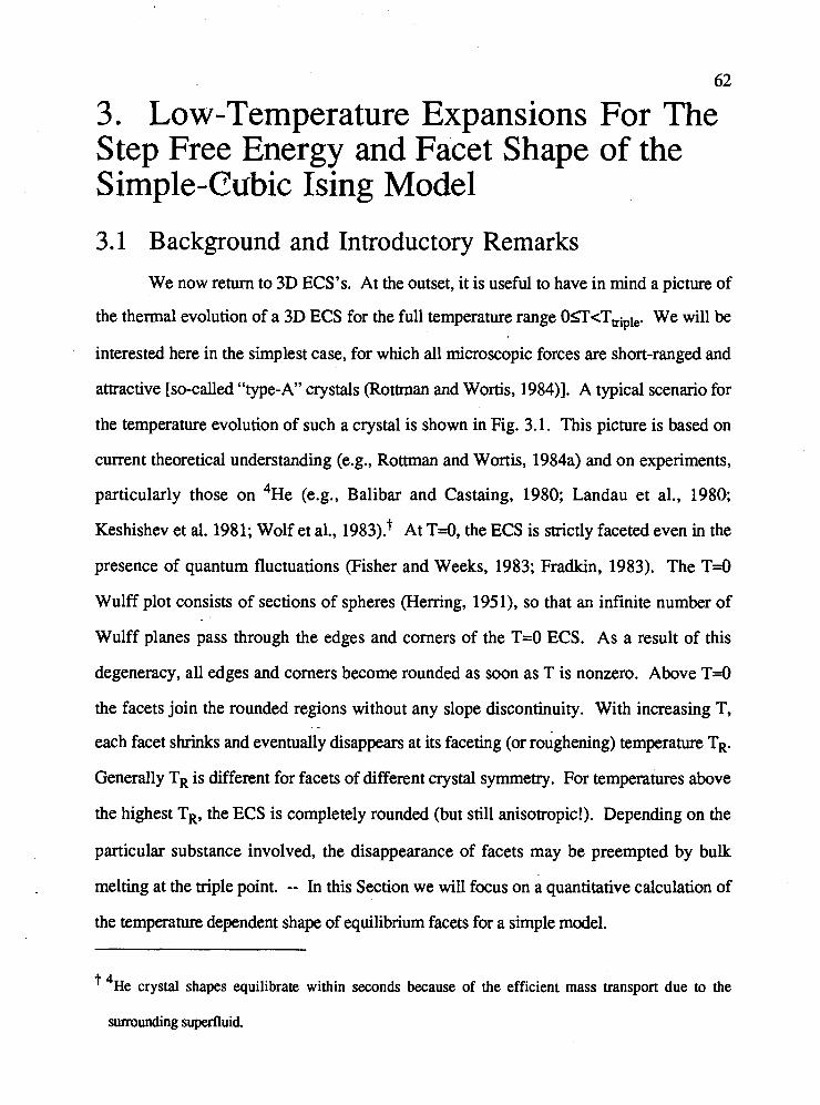
3. Low-Temperature Expansions Step Free Energy and Facet Shape

For The of the

Simple-Cubic Ising Model

3.1 Background and Introductory Remarks We now return to 3D ECS's. At the outset, it is useful to have in mind a picture of

the thermal evolution of a 3D ECS for the full temperature range OIT<T,iple. We will be

interested here in the simplest case, for which all microscopic forces are short-ranged and

attractive [so-called "type-A" crystals (Rottman and Wortis, 1984)l. A typical scenario for

the temperature evolution of such a crystal is shown in Fig. 3.1. This picture is based on

current theoretical understanding (e.g., Rottman and Wortis, 1984a) and on experiments,

particularly those on 4 ~ e (e.g., Balibar and Castaing, 1980; Landau et al., 1980;

Keshishev et al. 1981; Wolf et al., 1983)? At T=O, the ECS is strictly faceted even in the

presence of quantum fluctuations (Fisher and Weeks, 1983; Fradkin, 1983). The T=O

Wulff plot consists of sections of spheres (Herring, 1951), so that an infinite number of

Wulff planes pass through the edges and corners of the T=O ECS. As a result of this

degeneracy, all edges and corners become rounded as soon as T is nonzero. Above T=O

the facets join the rounded regions without any slope discontinuity. With increasing T,

each facet shrinks and eventually disappears at its faceting (or roughening) temperature TR.

Generally TR is different for facets of different crystal symmetry. For temperatures above

the highest TR, the ECS is completely rounded (but still anisotropic!). Depending on the

particular substance involved, the disappearance of facets may be preempted by bulk

melting at the triple point. -- In this Section we will focus on a quantitative calculation of

the temperature dependent shape of equilibrium facets for a simple model.

' 4 ~ e crystal shapes equilibrate within seconds because of the efficient mass transport due to the

surrounding superfluid.

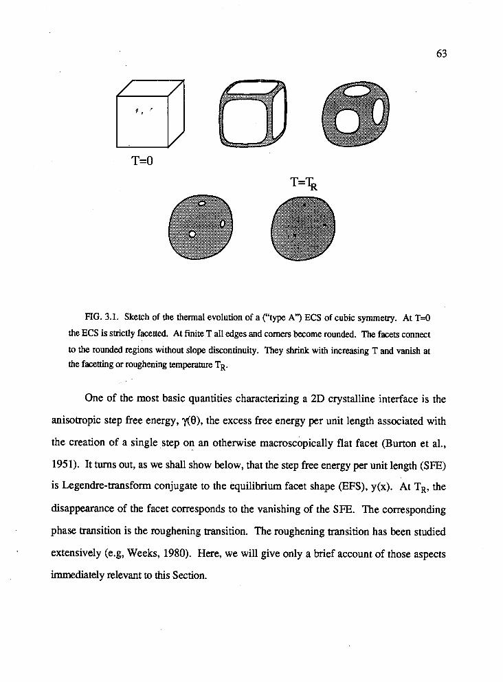
FIG. 3.1. Sketch of the thermal evolution of a ("type An) ECS of cubic symmetry. At T=O

the ECS is strictly facetted. At finite T all edges and corners become rounded. The facets connect

to the rounded regions without slope discontinuity. They shrink with increasing T and vanish at

the facetting or roughening temperature TR.

One of the most basic quantities characterizing a 2D crystalline interface is the

anisotropic step free energy, y(B), the excess free energy per unit length associated with

the creation of a single step on an otherwise macroscopically flat facet (Burton et al.,

1951). It turns out, as we shall show below, that the step free energy per unit length (SFE)

is Legendre-transform conjugate to the equilibrium facet shape (EFS), y(x). At TR, the

disappearance of the facet corresponds to the vanishing of the SFE. The corresponding

phase transition is the roughening transition. The roughening transition has been studied

extensively (e.g, Weeks, 1980). Here, we will give only a brief account of those aspects

immediately relevant to this Section.

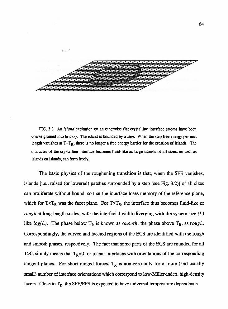
FIG. 3.2. An island excitation on an otherwise flat crystalline interface (atoms have been

coarse grained into bricks). The island is bounded by a step. When the step free energy per unit length vanishes at T=TR, there is no longer a free energy barrier for the creation of islands. The

character of the crystalline interface becomes fluid-like as large islands of all sizes, as well as

islands on islands, can fom freely.

The basic physics of the roughening transition is that, when the SFE vanishes,

islands [i.e., raised (or lowered) patches surrounded by a step (see Fig. 3.2)] of all sizes

can proliferate without bound, so that the interface loses memory of the reference plane,

which for T(TR was the facet plane. For T>TR, the interface thus becomes fluid-like or

rough at long length scales, with the interfacial width diverging with the system size (L)

like log(L). The phase below TR is known as smooth; the phase above TR, as rough.

Correspondingly, the curved and faceted regions of the ECS are identified with the rough

and smooth phases, respectively. The fact that some parts of the ECS are rounded for all

TM, simply means that TR=O for planar interfaces with orientations of the corresponding

tangent planes. For short ranged forces, TR is non-zero only for a finite (and usually

small) number of interface orientations which correspond to low-Miller-index, high-density

facets. Close to TR, the SFEIEFS is expected to have universal temperature dependence.

The model which has been very useful to study the universal character of the

roughening transitbn-is the so-called solid-on-solid (SOS) model. The SOS model is a

pure interface model (i.e., no bulk fluctuations are allowed), in which the interface is

represented by an array of stacks of "solids", the solids being cubes in the simplest case

(see Fig. 3.3). The ith stack consists of cubes up to some height hi, with no cubes above

hi and no vacancies below hi (hence the term SOS). A given configuration is then specified

by the set of heights {hi). The energy of a given configuration is taken to be a function of

the area of the "exposed" cube surfaces so that ~ s = ~ < i j > ~ ( l h i - h j l ) , where the sum is

over nearest neighbour pairs and V(x) is an increasing function of x (common choices are x

and x2). It is often a useful simplification to restrict the difference of the heights of

neighbouring stacks to be within a small range [e.g., for the body centred cubic restricted

SOS model, the difference is restricted to be k one solid (van Beijeren, 1977)l. The

resulting model is called the "restricted" SOS (RSOS) model. The SOS and RSOS models

are believed to capture the universal features of the roughening transition. While the SOS

model neglects bulk fluctuations (also called "bubbles" in this context), overhangs, and

handles (see Fig. 3.3), these excitations can in principle be integrated out with

renormalization flow to long length scales, because the bulk correlation length remains

finite at TR if TR(rc (Huse et al., 1985). The SOS model is dual to the XY model (Chui

and Weeks, 1976; van der Erdern and Knops, 1978; Swendsen, 1978). In precise analogy

to the duality statement of Eq. (2.3), the SFE, y(8,T), is just given by the inverse of the

XY correlation length, i.e.,

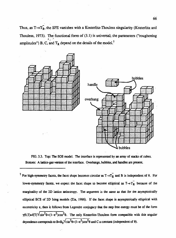
Thus, as T+T~, the SFE vanishes with a Kosterlitz-Thouless singularity (Kosterlitz and

Thouless, 1973). The functional form of (3.1) is universal; the parameters ("roughening t f '

amplitudes") B, C, and TR depend on the details of the model.'

\ bubbles

FIG. 3.3. Top: The.SOS model. The interface is represented by an array of stacks of cubes.

Bouom: A lattice-gas version of the interface. Overhangs, bubbles, and handles are present.

For high-symrnetq facets, the facet shape becomes circular as T+T;( and B is independent of 0. For

lower-symmetry facers, we expect the facet shape to become elliptical as T + T ~ because of the

marginality of the 2D lattice anisotropy. The argument is the same as that for the asymptotically

elliptical ECS of 2D Ising models (Zia, 1986). If the facet shape is asymptotically elliptical with

eccentricity E, then it follows from Legendre conjugacy that the step free energy must be of the form

~e,~fgdsin~0+(l-e2)cos2e. The only Kosterlitz-Thouless form compatible with this angular

dependarc corresponds m ~ = ~ ~ ~ s i n ~ ~ t ( l - ~ ~ ~ s ~ 0 and C a constant (independent of 0).

Exact solutions for the SFEEFS exist for RSOS models isomorphic to the 6-vertex

model (van Beijefen? 1977; Jayaprakash, et al., 1983; Jayaprakash and Saam, 1984a; I

~otecki , 1988). While these models show the expected universal XY-dual behaviour at

the roughening 'transition, they do not realistically model a true interface at lower

temperatures because of the neglect of overhangs and bubbles. These excitations, although

irrelevant in a renormalization-group sense, will alter the detailed, non-universal

temperature evolution of the SFE/EFS. An analytical calculation of y(0,T) for a more

realistic model which includes these excitations had not been performed prior to the work

presented here.

In this Section we develop a systematic low-temperature expansions of the SFE and

EFS for the simple-cubic (sc) nearest-neighbour Ising model. These expansions will allow

us to study in detail the effects of the excitations neglected in the SOS model. Our

expansion will make explicit use of the conjugacy between the SFE and the EFS. We

develop two expansions, one directly for the SFE (in the canonical ensemble) and one for

the EFS (in the grand canonical ensemble). The expansion for the SFE, y(B), about its

T=O cusps is divergent where the expansion of EFS is perfectly well behaved, and in that

sense the two expansions complement each other.

We focus on the sc Ising model not only because of its simplicity and its

fundamental importance to statistical mechanics but also because it allows us to make

contact with the work of others. In addition to recent Monte Carlo data (Mon et al., 1988,

1989) for y(B=O), low-temperature expansions by Weeks et al. in 1973 (see also Learny et

al., 1975) for the (100) facet of the sc Ising and the associated SOS model allow the

determination of the corresponding surface tensions T([100]) (Shaw and Fisher, 1989) and

roughening temperatures TR (Adler, 1987). The expansions of Weeks et al. involve the

combinatorics of finite clusters of adsorbed and/or desorbed atoms on an otherwise flat

interface. Here, we are faced with the more difficult problem of counting the

configurations available to these excitations in the presence of a step running across the 4 ,

interface. Because of the interactions of these excitations with the step and the many

degrees of freedom of the step itself, the complete combinatorics becomes exceedingly

involved. Fortunately, however, a large subset of configurations is in one-to-one

correspondence with those of the two-dimensional (2D) Ising ECS problem, for which we

have calculated the exact solution in the previous Section. We exploit this fact by

structuring the expansions for the SFEIEFS accordingly. While this simplifies our problem

considerably, the remaining combinatorics is still non-trivial.

We generate 5th and 1 lth order series for the SFE and the EFS, respectively. We

estimate convergence of these series for the symmetry directions to be better than 1% for

T<0.78TR. Normalizing the step free energy to the surface free energy of the facet, we

calculate the ratio of the facet diameter to the (100) diameter of the crystal. Below 0.72TR,

we find that the facet shape is given to better than 1% by the 2D Ising ECS. Corrections

due to overhangs and bubbles contribute less than 0.1% in this temperature region. Above

0.72TR the facet shape is essentially circular. From numerical extrapolations into the

critical region we obtain estimates for the roughening temperature and for the critical

amplitudes.

The remainder of this Section is organized as follows: In Sub-section 3.2 we give

the conceptual framework on which our expansions are founded. We derive the Legendre-

transform conjugacy between the SFE and the EFS, and show that the facet may be thought

of as a 2D ECS. We obtain expressions for the SFE and EFS in terms of a canonical and

grand canonical partition function, respectively. In Sub-section 3.3 we use the formalism

of the previous Subsection to calculate the step free energy and the shape of the (100) facet

of the sc Ising model. In Sub-section 3.4 convergence estimates for the low-temperature

series are developed. The feasibility of extracting critical parameters from the series is

discussed. The resu1,ts of such extrapolations are shown to be consistent with the Monte 2 5

Carlo estimates of Mon et al. (1988, 1989). We conclude in Sub-section 3.5.

3.2 Step free energies and facet shapes from interfacial free energies and equilibrium crystal shapes

As we have already seen in Fig 1.3, facets in the ECS arise from cusps of the Wulff A A

plot. Not just any cusp will do, however. Let the cusp be in the z direction and let m be

given in polar coordinates as shown in Fig. 3.4. Suppose that, at f led 6, the cusp has an

expansion for small $ given by

(1) r(0,$) = r(0.O) + r (0) $q + (higher order in $) ,

where q>O. Consider now the Wuiff construction at fixed 8. if the Wulff plane of the

cusp (the facet plane) intersects with the Wulff plane of r(8,$) in the limit as $+O at a

finite distance, x, from the cusp, then a facet with as smooth edge will be produced. From

the similar triangles of Fig. 3.4 it follows that the distance x is given by

Thus, a facet of finite extent exists only if the cusp is linear, i.e., if q=l. This means that,

if a cusp is to be conjugate to a facet with smooth edges, r(0,$) must have the Taylor

expansion,

ar r(0,q) = r(0.0) + [++, e) $ + (higher order in $) .

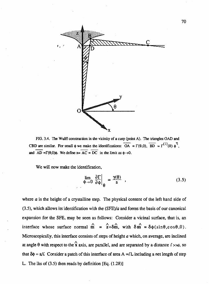
FIG. 3.4. The Wulff construction in the vicinity of a cusp (point A). The triangles OAD and - -

(1) CBD are similar. For small @ we make the identifications: OA = r(B,O), BD = r (8) @ , - -- and AD =r(8,0)@. We define x= AC = DC in the Iimit as $ 4 .

We will now make the identification,

where a is the height of a crystalline step. The physical content of the left hand side of

(3.3, which allows its identification with the (SFE)/a and forms the basis of our canonical

expansion for the SFE, may be seen as follows: Consider a vicinal surface, that is, an A A A A interface whose surface normal m = z+6m, with 6 m = 6+(sin8,cos0,0).

Microscopically, this interface consists of steps of height a which, on average, are inclined A

at angle 8 with respect to the x axis, are parallel, and are separated by a distance C >>a, so

that 641 = aK Consider a patch of this interface of area A =CL including a net length of step

L. The lhs of (3.5) then reads by definition [Eq. (1.28)]

where 0 denotes the Hamiltonian for a system with a single step of orientation 0 A

running across the facet of normal z. Eq. (3.6) will be the starting point for our canonical

expansion scheme for y(8). It emphasizes that the step free energy is defined in precise

analogy to the interfacial free energy [cf. Eq. (1.28)].

A simple but important consequence of the linear cusp (3.4) is that the 3D Wulff

construction for the ECS contains a 2D Wulff construction for the facet shape. Consider

again a cut trough the 3D Wulff construction at fixed 8 (see Fig. 3.5). We saw that, in

limit as $4, the line of intersection of the Wulff plane belonging to &(0,$) with the facet

plane occurs at perpendicular distance @)/a from the cusp. Since this is true for every

angle Q, these Bnes of intersection form a family of lines in the facet plane, each member of

which is at perpendicular distance y(8)la from the cusp. The facet shape is the interior

envelope of these lines because the ECS is the interior envelope of the corresponding

planes. This shows explicitly that the EFS is obtained as the 2D Wulff construction of a

polar plot of @)/a. This remrirkable fact, which allows us to think of facets as 2D ECS's

embedded in the surface of 3D ECS's was first pointed out by van Beijeren a d Nolden,

and also by Akutsu and Akutsu (1987b), in 1987. The physical explanation is simple:

Adjacent to the facet edge, the slope of the rounded region approaches zero, so steps

become widely separated in the thermodynamic limit. Thus, the edge of the facet may be

regarded microscopically as a single step encircling the (macroscopically) planar facet

region. The minimum-free-energy configuration of this step is given by the 2D Wulff

construction.

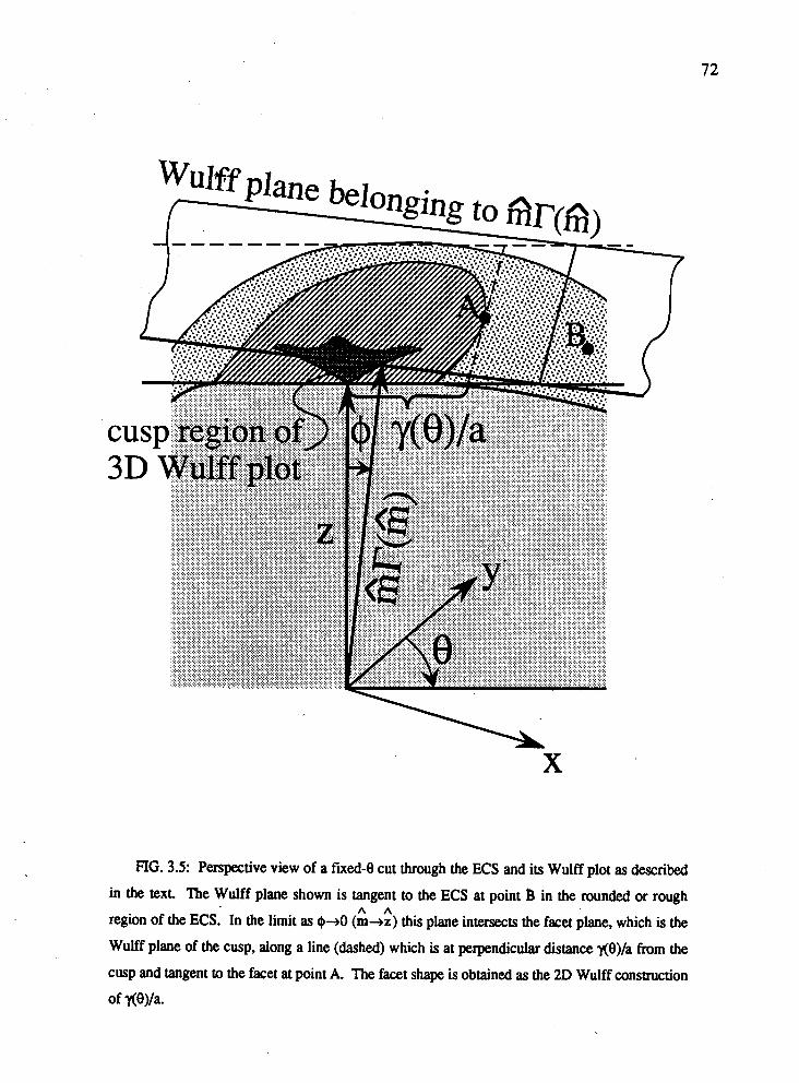
FIG. 3.5: Perspective view of a fixed8 cut through the ECS and its Wulff plot as described

in the text. The Wulff plane shown is tangent to the ECS at point B in the rounded or rough A A

region of the ECS. In the limit as $+O (m+z) this plane intersects the facet plane, which is the

Wulff plane of the cusp, along a line (dashed) which is at perpendicular distance *@la from the

cusp and tangent to the facet at point A. The facet shape is obtained as the 2D Wulff consauction

of y(8)la.

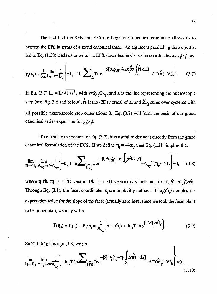
The fact that the SFE and EFS are Legendre-transform-conjugate allows us to

express the EFS in terms of a grand canonical trace. An argument paralleling the steps that

led to Eq. (1.38) leads us to write the EFS, described in Cartesian coordinates as yf(xf), as

In Eq. (3.7) Lx = L I ~ , with d y / a x f , and L is the line representing the microscopic

step (see Fig. 3.6 and below), is the (2D) normal of & and xe sums over systems with

all possible macroscopic step orientations 8. Eq. (3.7) will form the basis of our grand

canonical series expansion for yf(xf).

To elucidate the content of Eq. (3.7), it is useful to derive it directly from the grand

canonical formulation of the ECS. If we define qf = -hxp then Eq. (1.38) implies that

where q& (q is a 2D vector, tt% is a 3D vector) is shorthand for (qxf?+11,f)&b.

Through Eq. (3.8), the facet coordinates xf are implicitly defined. If pf(hd denotes the

expectation value for the slope of the facet (actually zero here, since we took the facet plane

to be horizontal), we may write

Substituting this into (3.8) we get f -I

While the sum in (3.10) extends over systems with all

possible interface krorifigurations, only those with vicinal surfaces contribute in the limit

q+qr We can, therefore, restrict the ensemble to the subspace of systems which have a

single step running across the facet of interest, i.e., we take z&)+zO and q&)+%,e. A strip of the interface of such a system of width L, is shown in Fig. 3.6, projected onto

A the xy-plane. Am=O everywhere on the interface except on the "cliffs" of height a

(represented by lines in the figure). We may, therefore, write for the field term of Eq.

(3.10)

where we have taken advantage of the fact that the integral lslhd.S over a close surface

vanishes. Substituting this into (3.10) and noting that the q term is independent of step Y

configuration establishes (3.7) without any direct reference to $0).

Eqs. (3.6) and (3.7) give the size of the facet at given h. Experimentally, however,

we would like to know the coordinates of the facet relative to the physical size of the

crystal. As a theoretically convenient and experimentally well defined measure of the

crystal size, we take the centre-of-crystal ("Wulff's point", Liebmann, 1914) to centre-of- A

facet distance, which is simply T(mf)/h [cf. Eq. (1. N)]. The relative facet coordinates

Finally, we remark that, for some intervals of 0, the facet plane may be

discontinuously truncated by Wulff planes from a part of the Wulff plot distant from the

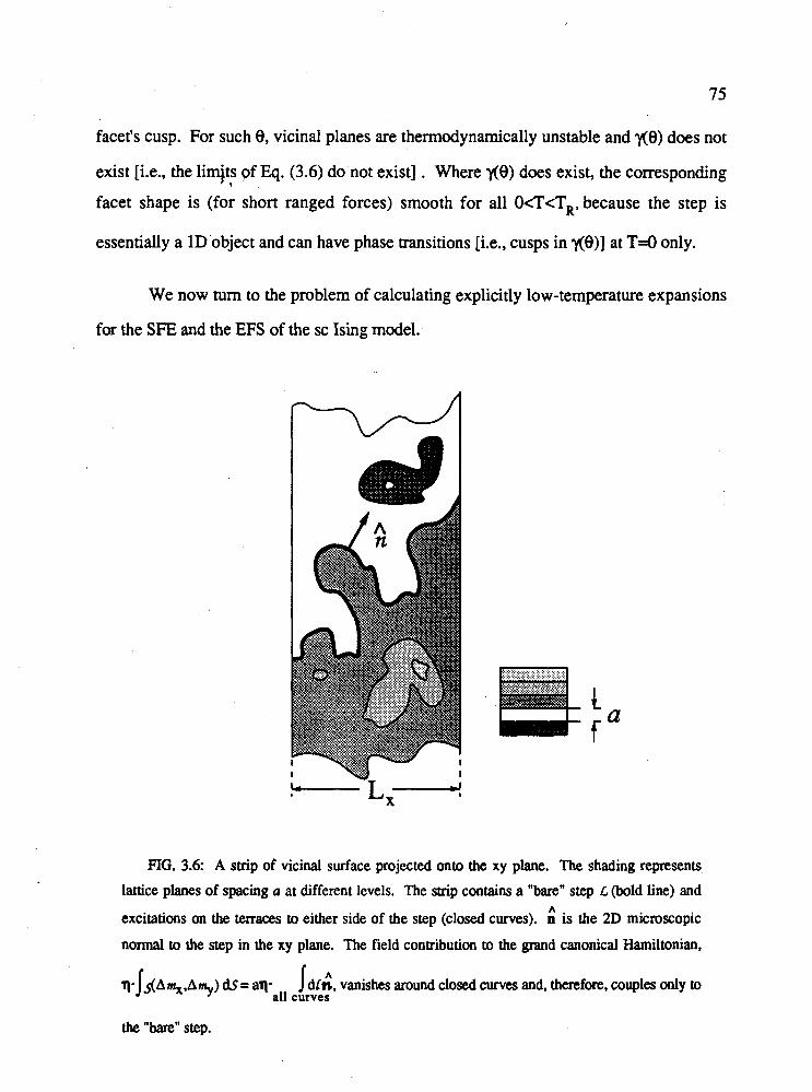
facet's cusp. For such 8, vicinal planes are thermodynamically unstable and y(8) does not

exist [i.e., the l iq t s of Eq. (3.6) do not exist] . Where y(8) does exist, the corresponding !

facet shape is (for short ranged forces) smooth for all OcTcT,, because the step is

essentially a 1D'object and can have phase transitions [i.e., cusps in y(8)] at T=O only.

We now turn to the problem of calculating explicitly low-temperature expansions

for the SFE and the EFS of the sc Ising model.

FIG. 3.6: A strip of vicinal surface projected onto the xy plane. The shading represents

lattice planes of spacing a at different levels. The strip contains a "bare" step L (bold line) and A

excitations on the terraces to either side of the step (closed curves). n is the 2D microscopic

normal to the step in the xy plane. The field contribution to the grand canonical Harniltonian,

-q A = a Id[& vanishes around closed curves andy therefore, couples only to all curves

the "bare" step.

3.3 Low-Temperature Series for the SFEJEFS of the simple-cubic Ising model

# f '

The Hamiltonian of the nearest-neighbour sc Ising model is

where the "spins", o. = f 1, are located at the vertices of a simple-cubic lattice of lattice J

constant a and the sum is over nearest-neighbur pairs. To keep our equations uncluttered

in the remainder of this Section, we shall set the overall scale factor ha3/~=l and measure

lengths in units of a, temperature in units of J h , and energy in units of J. (We shall also

drop the subscripts on xf and yf from here on.) In the lattice-gas interpretation of (3.13),

a. = +1 means that site j is occupied (by an "atom"); o. = -1 means site that j is vacant. J J

This model has a bulk phase transition at PC = 0.221655 (Pawley et al., 1984). For TcTc

there may be a first-order interface between a predominantly 4 = +I phase and a

predominantly- a = -1 phase. The ECS is a cube at T=O. For O<T<TR all interface j

orientations are expected to be stable (Rottman and Wortis, 1984b). At T=O the (100) facet

consists of a plane of bonds between spins of opposite sign. As T increases, fluctuations

are excited as spins flip in the bulk (gas atoms and vacancies) and on the interface (ad- and

desmbed atoms). Just as in Section 2, this is most easily visualized not in terms of broken

bonds but in terms of their dual-lattice plaquettes. Each plaquette corresponds to a unit of

interfacial area and costs energy 2 (i.e., 2J).

In order to study a step on a (100) interface, we need to make appropriate changes

in the Harniltonian (3.13). Consider the Ising system as filling a box of volume V and

height L, in which (100) lattice planes of area A are stacked at z = f 1/2, f 3/2, f 512,-.

To eliminate wall energies and to enforce a (100) interface, connect the box periodically in

the x and y directions and antiperiodically in the z direction. The (100) interface can be

stabilized at z=0 by applying an infinitesimal external symmetry breaking field, as I , '

described, for example, by Weeks et al. in 1973. The ground state of this interface is a

plane of plaquettes at z=0. Let the coordinates of the dual lattice sites in this plane be given

by two integers (nx,n ). We now modify the lattice by piercing it with two screw Y

A A dislocations of Burgers vector +z at (0,O) and -z at (N,M). This forces a step into the

interface running from (0,O) to (N,M) at average angle 8=arccos(N/L) with length

Between the dislocations, this step divides the interface into an upper and a

lower terrace. We choose to enforce the step in this manner (rather than by boundary

conditions) for combinatorical reasons. We envision the ground state of the interface with

this step to be planar everywhere except for the "tear" consisting of the INI+IMlrK extra

plaquettes constituting the shortest possible step from (0,O) to (N,M). This state has

degeneracy ~&N,M)=(&), because the step may stride IN1 times in the x direction and

IMI times in the y direction in any order (Fig. 3.7a). As T increases, atoms ad- and desorb

on the facet and the step will begin to lengthen and to develop overhangs (Fig. 3.7b). The

total free energy of this system will have contributions scaling like V from the bulk, like A

from the (100) interface, like L from the step, and like L, from the screw dislocations, plus

end effects of order unity from-the regions where the step terminates. Since we wish to

extract the step free energy, we must also subtract the screw-dislocation contribution in

addition to the bulk and surface terms already subtracted in Eqs. (3.6b) and (3.7). It turns

out that the screw dislocations do not contribute to the orders considered in our calculation.

Thus, we absorb them, for notational convenience, in the bulk free energy term, i.e., L

f + f + 2 2 fmew, where they can henceforth be ignored. b b V

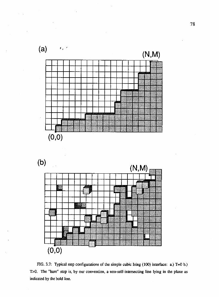
FIG. 3.7: Typical step configurations of the simple cubic Ising (100) interface: a.) T=O b.)

T>O. The "bare" step is, by our convention, a non-self-intersecting line lying in the plane as

indicated by the bold line.

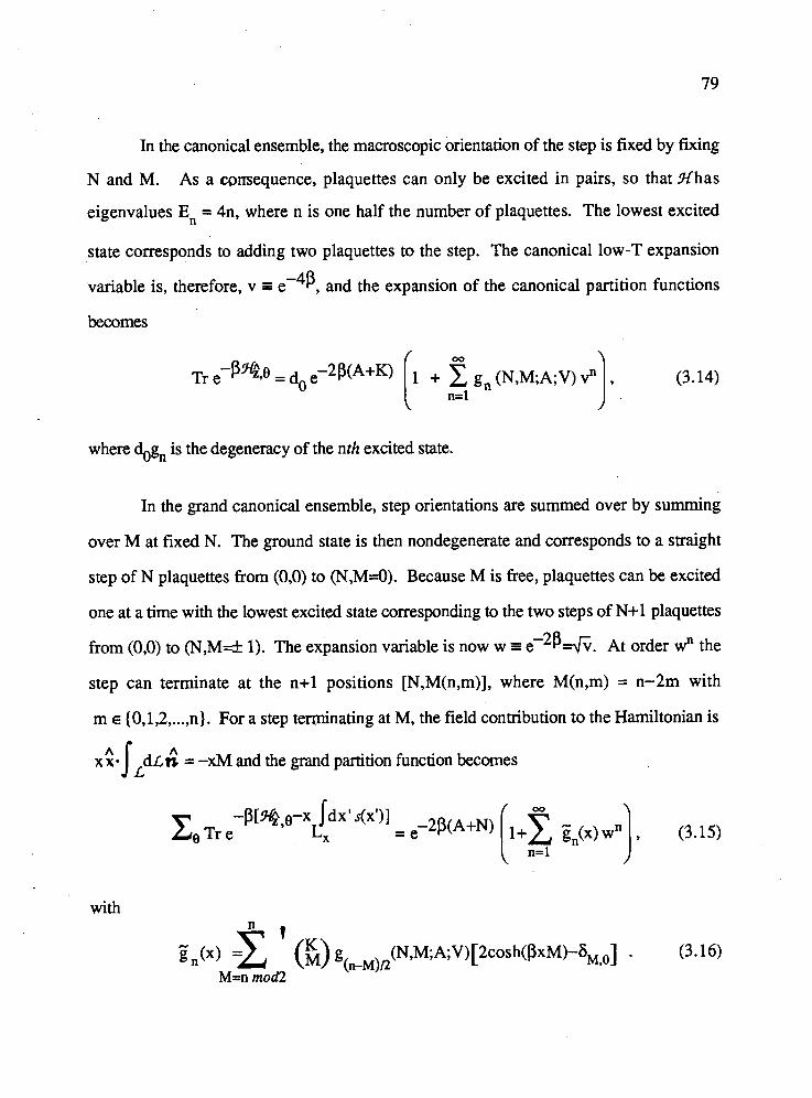
In the canonical ensemble, the macroscopic orientation of the step is fixed by fixing

N and M. As a cpnsequence, plaquettes can only be excited in pairs, so that Hhas

eigenvalues En = 4n, where n is one half the number of plaquettes. The lowest excited

state corresponds to adding two plaquettes to the step. The canonical low-T expansion

variable is, therefore, v r e-4P, and the expansion of the canonical partition functions

becomes

where Qg, is the degeneracy of the nth excited state.

In the grand canonical ensemble, step orientations are summed over by summing

over M at fixed N. The ground state is then nondegenerate and corresponds to a straight

step of N plaquettes from (0,O) to (N,M=O). Because M is free, plaquettes can be excited

one at a time with the lowest excited state corresponding to the two steps of N+l plaquettes

from (0,O) to ( N M d 1). The expansion variable is now w I e-2P6v. At order wn the

step can terminate at the n+l positions [N,M(n,m)], where M(n,m) = n-2m with

m E (0,1,2, ..., n). For a step terminating at M, the field contribution to the Hamiltonian is

A x:-I d L n = -xM and the grand partition function becomes L

with

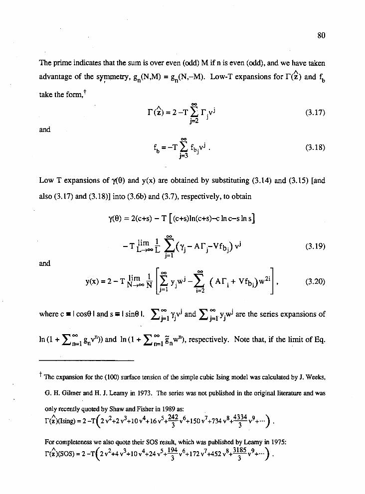
The prime indicates that the sum is over even (odd) M if n is even (odd), and we have taken A

advantage of the sympetry, gn(N,M) = gn(N,-M). Low-T expansions for r ( z ) and fb I

take the form:

and

Low T expansions of y(8) and y(x) are obtained by substituting (3.14) and (3.15) [and

also (3.17) and (3.1 8)] into (3.6b) and (3.7), respectively, to obtain

y(e) = 2(c+s) - T [(c+s)ln(c+s)-c in c-s in s]

where c = I cose I and s I I sine I. z y y.vJ and z ~ l Y j ~ j are the series expansions of ~1 J

In (1 + z:l gnvn)) and in (1 + zzl &,wn), respectively. Note that, if the limit of Eq.

' The expansion for the (100) surface tension of the simple cubic Ising model was calculated by J. Weeks,

G. H. Gilmer and H. J. Leamy in 1973. The series was not published in the original literature and was

only recently quoted by Shaw and Fisher in 1989 as: A 5 242 6 7 r(z)(Ising) = 2 -T 2 v2+2 v3+10 v4+16 v +-v +I50 v +734 v 3

For completeness we also quote their SOS result, which was published by Leamy in 1975: A r ( ~ )(SOS) = 2 -T 2 v2+4 v3+ 10 v4+24

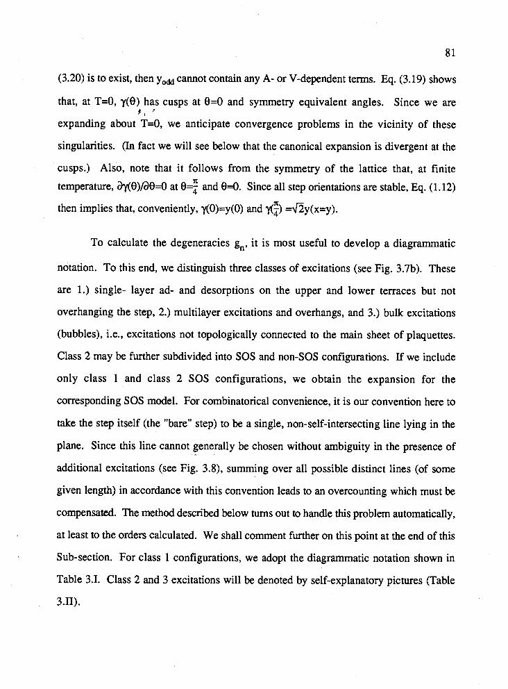
(3.20) is to exist, then yodd cannot contain any A- or V-dependent terms. Eq. (3.19) shows

that, at T=O, y(8) has cusps at 8=0 and symmetry equivalent angles. Since we are + '

expanding about T=O, we anticipate convergence problems in the vicinity of these

singularities. (In fact we will see below that the canonical expansion is divergent at the

cusps.) Also, note that it follows from the symmetry of the lattice that, at finite

temperature, a'~(8)/a8=0 at 8$ and 8=0. Since all step orientations are stable, Eq. (1.12)

then implies that, conveniently, y(O)=y(O) and x:) d2y(x=y).

To calculate the degeneracies g,, it is most useful to develop a diagrammatic

notation. To this end, we distinguish three classes of excitations (see Fig. 3.7b). These

are 1.) single- layer ad- and desorptions on the upper and lower terraces but not

overhanging the step, 2.) multilayer excitations and overhangs, and 3.) bulk excitations

(bubbles), i.e., excitations not topologically connected to the main sheet of plaquettes.

Class 2 may be further subdivided into SOS and non-SOS configurations. If we include

only class 1 and class 2 SOS configurations, we obtain the expansion for the

corresponding SOS model. For combinatorical convenience, it is our convention here to

take the step itself (the "bare" step) to be a single, non-self-intersecting line lying in the

plane. Since this line cannot generally be chosen without ambiguity in the presence of

additional excitations (see Fig. 3.8), summing over all possible distinct lines (of some

given length) in accordance with this convention leads to an overcounting which must be

compensated. The method described below turns out to handle this problem automatically,

at least to the orders calculated. We shall comment further on this point at the end of this

Sub-section. For class 1 configurations, we adopt the diagrammatic notation shown in

Table 3.1. Class 2 and 3 excitations will be denoted by self-explanatory pictures (Table

3.11).

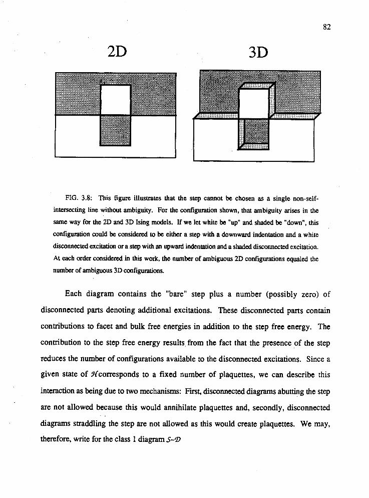
FIG. 3.8: This figure illustrates that the step cannot be chosen as a single non-self-

intersecting line without ambiguity. For the configuration shown, that ambiguity arises in the

same way for the 2D and 3D Ising models. If we let white be "up" and shaded be "down", this

configuration could be considered to be either a step with a downward indentation and a white

disconnected excitation or a step with an upward indentation and a shaded disconnected excitation.

At each order considered in this work, the number of ambiguous 2D configurations equaled the

number of ambiguous 3D configurations.

Each diagram contains the "bare" step plus a number (possibly zero) of

disconnected parts denoting additional excitations. These disconnected parts contain

contributions to facet and bulk free energies in addition to the step free energy. The

contribution to the step free energy results from the fact that the presence of the step

reduces the number of configurations available to the disconnected excitations. Since a

given state of Hcorresponds to a fixed number of plaquettes, we can describe this

interaction as being due to two mechanisms: First, disconnected diagrams abutting the step

are not allowed because this would annihilate plaquettes and, secondly, disconnected

diagrams straddling the step are not allowed as this would create plaquettes. We may,

therefore, write for the class 1 diagram S-D

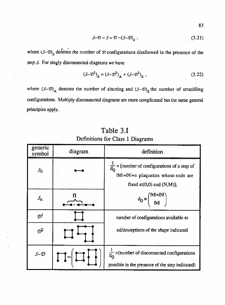
where (S-CD)~ deht& the number of I) configurations disallowed in the presence of the

step S. For sing!y disconnected diagrams we have

(s-I)')~ = ( s - d ) ~ + ( ~ - 9 ~ ) ~ , (3.22)

when (S-I))A denotes the number of abutting and (s-I))), the number of straddling

configurations. Multiply disconnected diagrams are more complicated but the same general

principles apply.

Table 3.1 Definitions for Class 1 Diagrams

diagram definition

- x [number of configurations of a step of

IMI+INl+n plaquettes whose ends are

fixed at(0,O) and (N,M)];

number of configurations available to

ad/desorptions of the shape indicated

1 - number of disconnected configurations do possible in the presence of the step indicated)

If we were to allow only desorptions on the upper terrace level and adsorptions on

the lower, interface configurations would be isomorphic to those of the 2D square Ising f , '

model with an interface between "up" and "down9' phases in lieu of the step. Although the

symmetry of Hbetween ad- and desorptions destroys this isomorphism, we can still take

advantage of the exact 2D solution for the interfacial free energy, r2D(0), and for the ECS,

~ ~ ~ ( x ) , t o simplify the full 3D combinatorics. Note that class 1 diagrams can equally well

be used in the expansion of r2D(0) and y2,(x), if we ignore the fact that they are to

represent both ad- and desorptions. In 2D, the nature of the "interaction" between

disconnected parts and the step remains unchanged from 3D (dual-lattice bonds replacing

dual-lattice plaquettes), so Eqs. (3.21) and (3.22) hold also for the 2D interpretation of the

diagrams. For singly disconnected diagrams ( ~ - b ) , ~ ~ = 2 ( S - D ' ) ~ ~ ~ . as both ad- and

desorptions can straddle the step. However, Sand (S-b)* have the same value, whether

interpreted as 2D or 3D configurations, because adsorptions (desorptions) are allowed to

abut the step on the upper (lower) terrace. This allows us to shift the necessity for doing

the explicit coinbinatorics of many 2D configurations up by several orders from where they

fmt occur by writing

and 00

lim I Y(X) = - L +- L

- [A(ri-f2Dbii * vfb.] w2j (3.25) 1

i=2

In these equations Y2Di and Y2Di are the 2D versions of yi and yi, respectively, i.e., they

are the terms in Eqs. (3.19) and (3.20) arising from the 2D interpretation of class 1 2 , '

diagrams. fiDb is the 2D bulk free energy for the 2D Ising model. The effect of this

rearrangement is that many terms cancel in the curly brackets of (3.23) and (3.25), so that

the number of diagrammatic terms corresponding to Ayi and Ayi, which remain to be

evaluated is significantly reduced (at least at low orders). This is a tremendous

simplification, as the order-by-order calculation of S and (S"D)* diagrams is exceedingly

tedious. Also, all terms involving A and V vanish, as is necessary if the thermodynamic

limit L+- is to exist. Because these terms cancel, the Ayi and Ayi can be expressed

entirely in terms of the A- and V-independent parts of gi and gzDi . If ai, Agi, gi, and A&

denote the A- and V-independent parts of gzD , (gi - g .), HzDi and (gi -E2Di), i 2%

respectively, we can, therefore, simply write

and

It is crucial here that ai, Agi, a", and Agi contain not only the terms of order L', but also

those of order Lo, since the latter get multiplied by order L' terms at higher order in the

expansion of the logarithms. The nonvanishing a's and Ag's needed in (3.27) for the

calculation of the Ayi to order 5, inclusively, have the diagrammatic expansions,

a, = (1) t , '

a, = (111)-(11)

where the numbers in brackets label diagrams listed (with their numerical equivalents) in

Table 3.II (some combinatorical details are given in Appendix E). The corrections Ayi can

now be evaluated to 1 l th order without calculating additional diagrams. The expansions of

the necessary nonvanishing and A& are simply obtained by appropriate substitution into

Eq. (3.16) (put g=a to evaluate Z and g=Ag to evaluate ~ g ) .

To the orders calculated here, the method of expansion described above solves the

problems associated with the ambiguity of defining the step as a single, non-self-

intersecting line (Fig. 3.8). We find that, with consistent use of that definition, diagrams

conspire such that the number of overcounted configurations is the same for the 2D model

as it is for the 3D model, so that they cancel in the calculation of the Agi . This cancellation

is transparent for simple diagrams such as shown in Fig. 3.8. It can be checked to occur at

the orders considered in this work; whether it persists to all orders is unclear.

The calculation of the diagrams appearing in the grand canonical expansion is easier (at least at low

orders) than the calculation of the canonical diagrams, in the sense that the former, unlike the latter, need

not be calculated for general M. This fact may be useful to push our calculation to higher order to get

more information in the critical region. Since the facet is essentially isotropic there, the fact that the

grand canonical series converges best in only one symmetry direction (&0) is not a serious limitation.

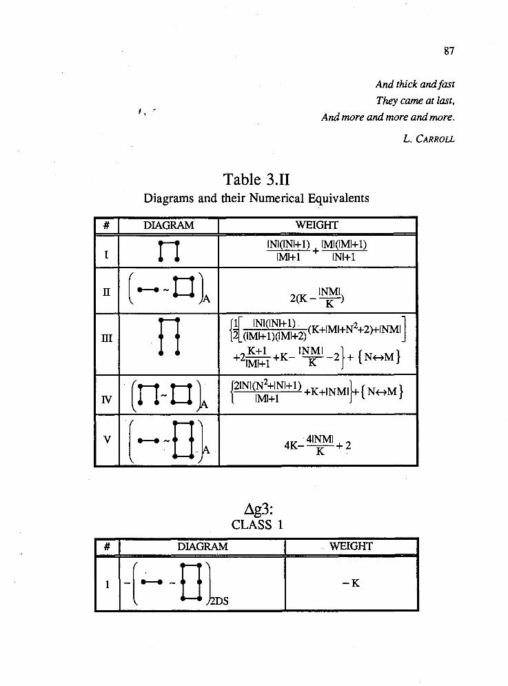
t , '

And thick and fast They came at last,

And more and more and more.

Table 3.11 Diagrams and their Numerical Equivalents

DIAGRAM I WEIGHT

~'N'(N~+~N'+') +K+INMI ( NwM [n- n lg i lMl+l I + )

Ag3: CLASS 1

WEIGHT

- K

# DIAGRAM

-[LmulDs

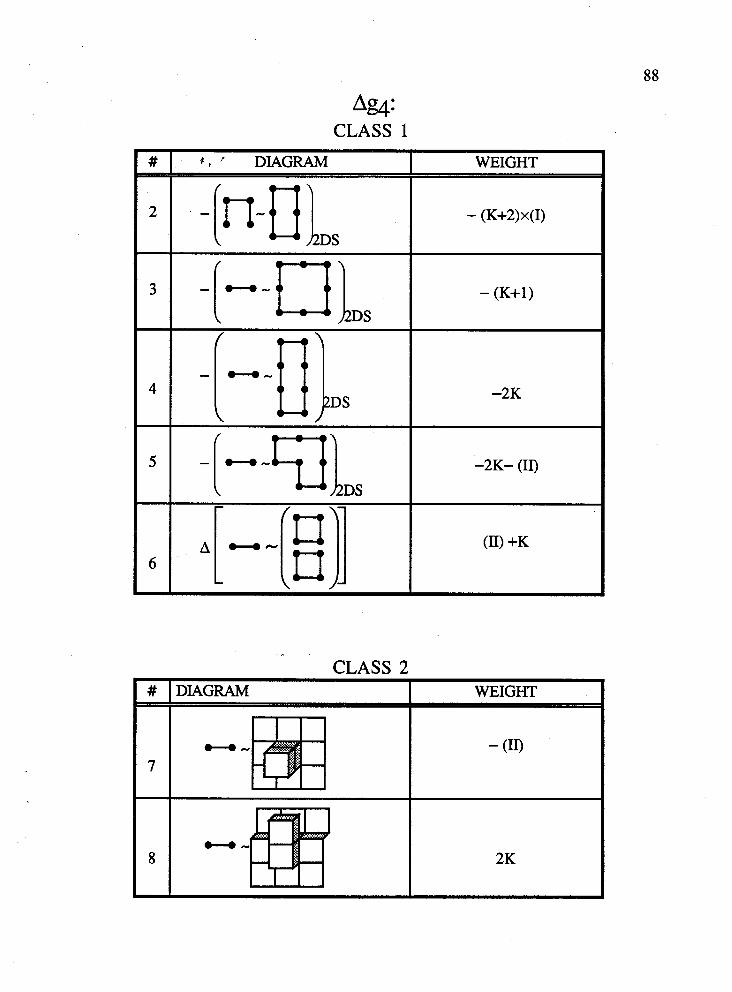
A&: CLASS 1

f , - DIAGRAM I WEIGHT

-2K- (11)

CLASS 2 DIAGRAM WEIGHT

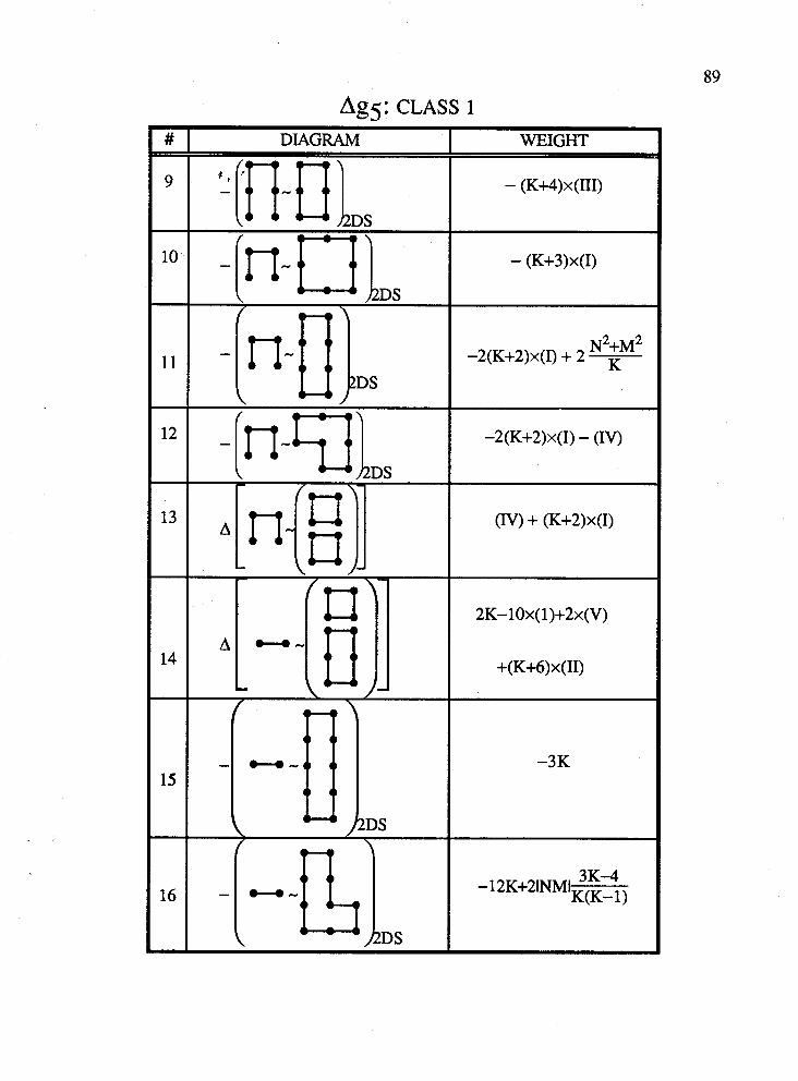
Ag5: CLASS 1

DIAGRAM WEIGHT

-2(K+2)~(1) - (IV)

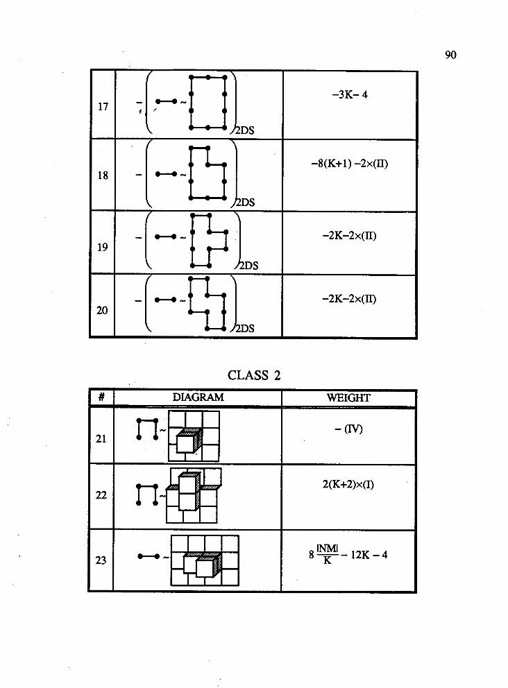
I # I DIAGRAM

CLASS 2

WEIGHT

2(K+2)x (I)

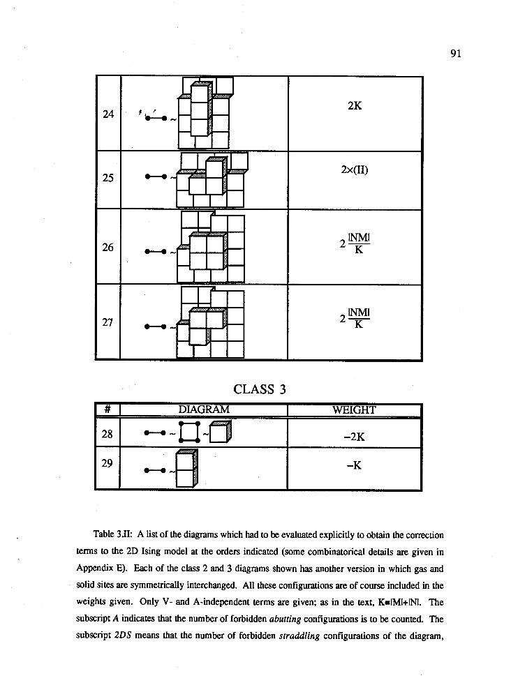
CLASS 3

Table 3.m A list of the diagrams which had to be evaluated explicitly to obtain the correction

terms to the 2D Ising model at the orders indicated (some combinatorical details are given in

Appendix E). Each of the class 2 and 3 diagrams shown has another version in which gas and

solid sites are symmetrically interchanged. All these configurations are of course included in the

weights given. Only V- and A-independent terms are given; as in the text, K=IMI+INI. The

subscript A indicates that the number of forbidden abutting configurations is to be counted. The

subscript 2DS means that the number of forbidden straddling configurations of the diagram,

#

28

29

DIAGRAM

w- tJ===J w-

WEIGHT

-2K

-K

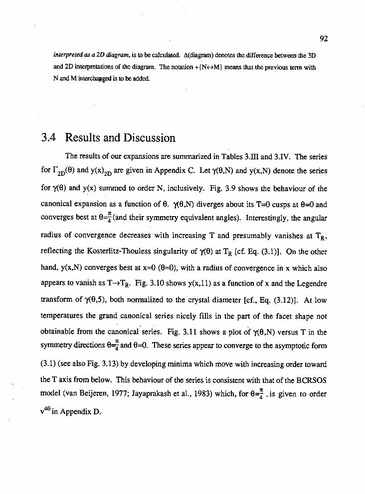
interpreted as a 2 0 diagram, is to be calculated. A(diagram) denotes the difference between the 3D

and 2D interpretations of the diagram. The notation + (Nt+M) means that the previous term with

N and M interchqged is to be added.

3.4 Results and Discussion

The results of our expansions are summarized in Tables 3.111 and 3.IV. The series

for r2D(8) and Y(x)~D are given in Appendix C. Let y(8,N) and y(x,N) denote the series

for y(8) and y(x) summed to order N, inclusively. Fig. 3.9 shows the behaviour of the

canonical expansion as a function of 8. y(8,N) diverges about its T=O cusps at 8=0 and

converges best at 8< (and their symmetry equivalent angles). Interestingly, the angular

radius of convergence decreases with increasing T and presumably vanishes at TR,

reflecting the Kosterlitz-Thouless singularity of y(8) at TR [cf. Eq. (3.1)]. On the other

hand, y(x,N) converges best at x=O (8=0), with a radius of convergence in x which also

appears to vanish as T+TR. Fig. 3.10 shows y(x,ll) as a function of x and the Legendre

transform of y(8,5), both normalized to the crystal diameter [cf., Eq. (3.12)]. At low

temperatures the grand canonical series nicely fills in the part of the facet shape not

obtainable from the canonical series. Fig. 3.1 1 shows a plot of y(8,N) versus T in the

symmetry directions 8< and 8=0. These series appear to converge to the asymptotic form

(3.1) (see also Fig. 3.13) by developing minima which move with increasing order toward

the T axis from below. This behaviour of the series is consistent with that of the BCRSOS

model (van Beijeren, 1977; Jayaprakash et al., 1983) which, for 0: .is given to order

v40 in Appendix D..

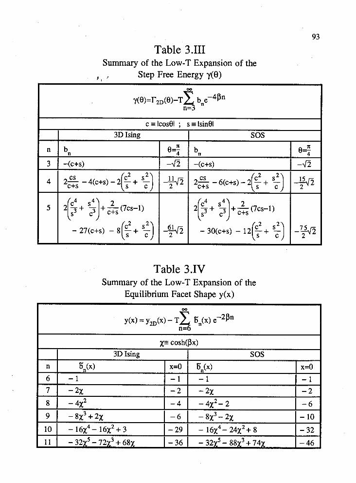
Table 3.111 Summary of the Low-T Expansion of the

9 , Step Free Energy y(8)

3D Ising SOS

Table 3.IV Summary of the Low-T Expansion of the

Equilibrium Facet Shape y(x)

x= cosh(px)

n

6 7

8

9

10

11 I -32r5-72r3+68r I - 36 I - 32r5 - 88r3 + 74r 1-46

3D Ising

sn(x) - 1

- 2x - 4x2

- gx3 + 2~

-16x4-16x2+3

SOS x=O

- 1 - 2

- 4

- 6

-29

En(x) - 1

- 2x - 4x2- 2

- gX3 - 2x

-16x4-24x2+8

x=O

- 1 - 2

- 6

- 10

- 32

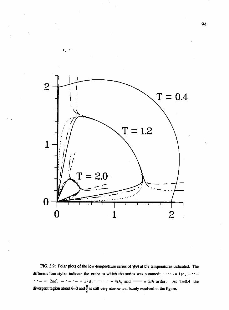
FIG. 3.9: Polar plots of the low-temperature series of 1(8) at the temperatures indicated. The

different line styles indicate the order to which the series was summed: . . - . - - l s t * - . . - . . - = 2nd, - . - - - = 3rd, - - - - = 4th, and - - - 5th order. At T-0.4 the

divergent region about 030 and: is still very narrow and bmly resolved in the figure.

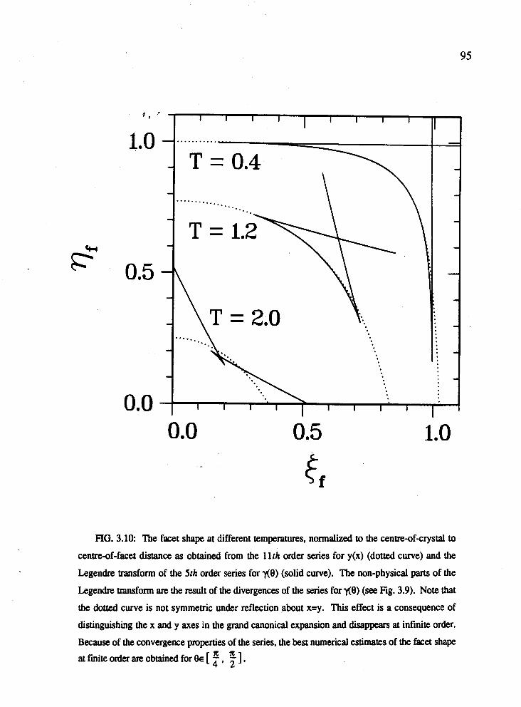
FIG. 3.10: m e facet shape at different temperatures, normalized to the centre-of-crystal to

cenm-of-facet distance as obtained from the 1 l th order series for y(x) (dotted curve) and the

Legendre transform of the 5th order series for $8) (solid curve). The non-physical parts of the

Legendre transform are the result of the divergences of the series for y(8) (see Fig. 3.9). Note that

the dotted curve is not symmetric under reflection about x=y. This effect is a consequence of

distinguishing the x and y axes in the grand canonical expansion and disappears at infinite order.

Because of the convergence properties of the series, the best numerical estimates of the facet shape

at fmite order are obtained for & [ f , f 1.

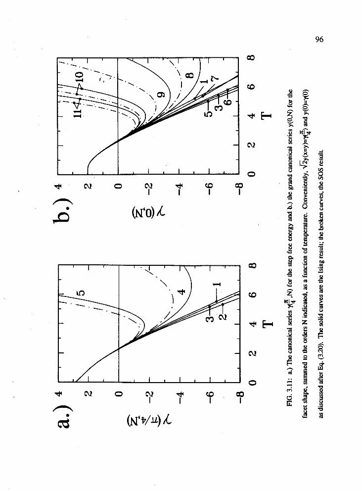
To investigate the asymptotic properties of our series, standard Pad6 and ratio

methods (e.g., Gaunt and Guttmann, 1974) cannot be used directly because the singularity 4 , f

of Eq. (3.1) is an essential singularity. Since there is no obvious way of circumventing

this problem, we use alternate methods, motivated mainly from a study of the exact

solution of the BCRSOS model. The low-T series for $) of the BCRSOS model (see

Appendix D) is an alternating series: Order v is negative, orders v2 to v10 are positive,

orders vl' to v3' are negative, and so on. The number of consecutive terms of like sign

presumably increases with increasing order. For TS 0.85TR, the convergence of this series

is dominated by the first sequence of positive terms, i.e., the terms of order vn with

ntz {k,.. .,l) , where k=2 and b10 here. Let a, denote the coefficient of vn. It turns out that

the ratio rn q a,/a,-l, decreases with n for ne {k+l, ...,Oil! Hence, if T is sufficiently

low such that v rmcl , it follows that vrncl for n2m ( n , m ~ P) and, therefore,

j=O - the series x :=m+l anvn is bounded by the geomemc series ximvmxkm-l xj =

x h v m S(On), where x=v r,. Thus, if mccL a reasonable estimate for x n=m+l anvn is

We shall assume that the generic form of the complete series for the SFE of the sc

Ising model is similar to that of the corresponding series of the BCRSOS model. In order

to estimate the error made in truncating the series after order N, let us assume further that

the grand canonical series cannot converge significantly better than the canonical series, so R

that we can restrict our analysis to 0 7 . For the Ising and SOS models, the forgoing

paragraph then implies that it is reasonable to expect the series for the error R R

ANi~(z)-~(zN), for N24, to be bounded by a geometric series, so that

4 2 4 2 AN 5 Z N i -T p(bN+ $x/(1-x), provided Ocxcl, where x=v (bN+ e ) ~ ( b ~ - ~ + G) is

the ratio of the Nth to the (N-1)st term of ~ $ , N ) . While it is only clear that this must be

so at sufficiently low T, we shall assume that 3, gives a reasonable error estimate for

fractional errors3 l[Y(:,5)+35] as high as -10%. For N=5 we find that the fractional J , *

error is less than (0.1%,1%,5%,10%) for T I (1.72,1.92,2.04,2.09); for N=4 these

temperatures ari (1.61,1.78,1.87,1.90). For the SOS model the corresponding estimates

are for N=5, TI(l.73,1.93,2.07,2.12) and for N=4, TI(l.5 l,l.62,1.66,1.67).

If we take the fractional error in approximating y(0) by r,,(0) to be

1 - ~ ~ ~ ( 0 ) / [ ( ~ ( ~ , 5 ) + Z J , we find it to be less than 1% for Tc1.79 (less than 0.1% for

T4.51). Below T=1.79 the order v4 and v5 non-SOS contributions are less than 0.08%

and 0.03% respectively so that bubbles and overhangs are unimportant in this temperature

range. Above T=1.79, the facet-shape anisotropy, as approximated by

[y(~,5)-y(0,11)]/y(0,11), is less than 4 x 1 0 ~ ~ for both the Ising and SOS models. At

T=1.79, the normalized facet radius pf = 0.4. It follows that, in the region of temperature

where the facet has experimentally significant anisotropy (i.e., for T s 1.8), the facet shape

is essentially given by the 2 0 Ising ECS with the convergent corrections calculated in Sub-

section 3.3.

In the temperature range 1.8sT5 2.1, T is high enough for the the series to differ

significantly from the 2D lsing series but low enough for us still'to have some confidence

that the series have converged. Assuming that in this region y(:,5) and y(0,ll) are already

well approximated by their asymptotic form (3.1), one may hope to extract the critical

parameters B, C, and TR. Indeed, plots of C(T) I -~(T,-T) '~ alny(0,N)laT and It B ( T ) ~ ~ , N ) ~ x ~ [ c ( T ) / ~ ~ ~ versus T for various values of TR, at 0 ~ a n d 0, show a

plateau for TR=TPOateau)=2.46 over the temperature range 1.8-(r 2.0 (see Fig. 3.12). The

failure of the plateau to extend beyond T=2.0 is consistent with the convergence estimates

above. The functions B(T) and C(T) [which would be constants if the series were exactly

equal to (33)] have qualitatively the same shape (Fig. 3.12): For TR>TP, they increase

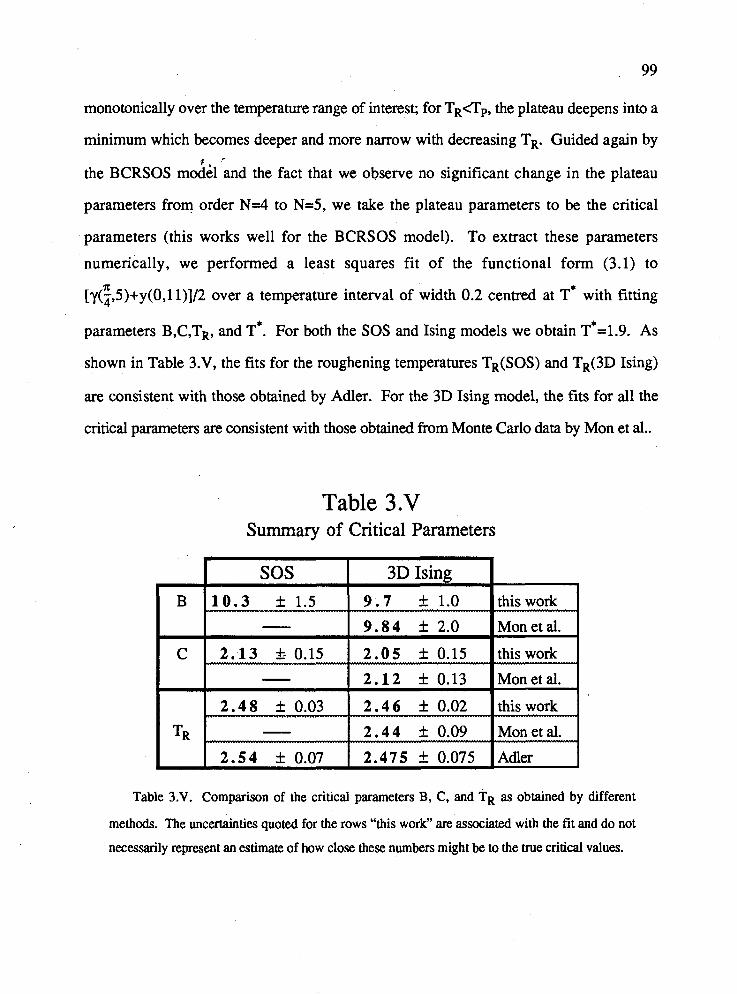
99

monotonically over the temperature range of interest; for TR+, the plateau deepens into a

minimum which becomes deeper and more narrow with decreasing TR. Guided again by +, '

the BCRSOS model and the fact that we observe no significant change in the plateau

parameters from order N=4 to N=5, we take the plateau parameters to be the critical

parameters (this works well for the BCRSOS model). To extract these parameters

numerically, we performed a least squares fit of the functional form (3.1) to

[y(~75)+y(0711)m over a temperature interval of width 0.2 centred at T* with fitting

parameters B,C,TR, and T*. For both the SOS and Ising models we obtain ~*=1.9. As

shown in Table 3.V, the fits for the roughening temperatures TR(SOS) and TR(3D Ising)

are consistent with those obtained by Adler. For the 3D Ising model, the fits for all the

critical parameters are consistent with those obtained from Monte Carlo data by Mon et al..

Table 3.V Summary of Critical Parameters

SOS 3D Ising I B 10 .3 f 1.5 9.7 1: 1.0 this work

C 2:13 k- 0.15 2.05 f 0.15 this work

- 2.12 1 0 . 1 3 Monetal.

2.48 + 0.03 2.46 f 0.02 this work

TR p. - 2.44 f 0.09 Monetal.

2.54 f 0.07 2.475 + 0.075 Adler

Table 3.V. Comparison of the critical parameters B, C, and TR as obtained by different

methods. The uncertainties quoted for the rows "this work" are associated with the fit and do not

necessarily represent an estimate of how close these numbers might be to the true critical values.

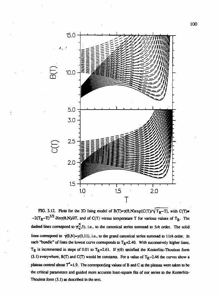
FIG. 3.12. Plots for the 3D Ising model of B O = ~ ( ~ , N ) ~ ~ ~ [ C ( T ) / ~ ~ , with C m

-z(T~-T)" alnHe,N)/aT, and of C(T) versus temperature T for various values of TR. The

dashed l k s correspond to $3, i.e., to the canonical series summed to 5th order. The solid

lines correspond to y@,N)=y(O,ll), i.e.. to the grand canonical series summed to 1 lth order. In

each "bundle" of lines the lowest curve corresponds to TR=2.40. With successively higher lines,

TR is incremented in steps of 0.01 to TR=2.61. If He) satisfied the Kosterlitz-Thouless form

(3.1) everywhere, B O and C O would be constants. For a value of TR-2.46 the curves show a

plateau centred about ~*=1.9. The corresponding values of B and C at the plateau were taken to be

the critical parameters and guided more accurate least-square fits of our series to the Kosterlitz-

Thouless form (3.1) as described in the text.

Fig. 3.13 shows the T dependence of the normalized facet diameter of the Ising

model, extrapolatqd aJ1 the way to TR using our fit to Eq. (3.1). The lower (upper) limit of I

the error bars shown there correspond to fits obtained over the interval 1.9051TS1.955

with TR constrained to be the lower (upper) limit of Adler's estimates for TR. It is to be

emphasized, that the methods of Sub-section 3.3 are not recommended if one is interested

in TR only (and not, for example, in the amplitudes B and C also). In such cases, the

series methods of Weeks et al., with their well understood asymptotic analysis by Adler,

are probably more efficient. The calculation presented here, on the other hand, is the only

one so far to address the anisotropic step free energy and the shape and size of facets.

It is interesting to examine the assumption that the series are already in the

asymptotic regime over the temperature range 1.8,Crs 2.1 in the context of the Monte Carlo

simulations of Mon. et al.. While their data, extrapolated to infinite system size, shows

(3.1) to hold over the entire temperature range 1.8(rcTR, they fall below the 2D Ising

value by about 10% at T=1.8, where our expansion implies that the 2D Ising result is a

lower bound. In principle, this discrepancy could be due to large negative coefficients at

higher orders of our expansion; however, in light of the discussion above, this is unlikely.

A more likely source of error, as pointed by Mon et al., is the finite-size-scaling analysis of

the Monte Carlo data, performed with only three data points at each value of T. The fact

that our critical parameters agree with those of Mon et al. in spite of these problems is

probably attributable to the sensitive dependence of $8) on the precise numerical values of

the critical parameters.

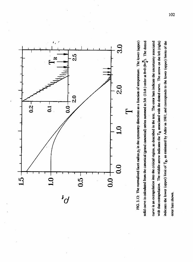
3.5 Conclusions

We have bh6wn how to calculate step free energies and the corresponding

equilibrium facet shapes in low-temperature expansion. The combinatorics involved is

significantly reduced by structuring these expansions as perturbation series about the

interfacial properties of the 2D Ising model. The two expansions are related by a Legendre

transform and can be thought of as canonical and grand canonical representations of the

same physics. The grand canonical form of the expansion gives the facet shape where it is

not accessible from the canonical expansion of the step free energy.

At temperatures where the facet has experimentally significant anisotropy, the facet

shape is essentially given by the 2D Ising ECS normalized to the facet's surface free

energy, with convergent corrections displayed in Tables 3.111 and 3.W. Corrections to the

2D Ising result due to additional (non-2D) SOS, overhanging, and bubble configurations

enter at orders e-12PJ, e-l6PJ, and e-20pJ, respectively. These corrections are less than I%

for 0<T<1.79=0.72TR and less than 0.1% for 0(r<1.51=0.61TR. In this temperature

range, overhangs and bubbles are unimportant. At higher temperatures the facet shape is

nearly circular, with a normalized facet radius of less than 0.4 and anisotropies of less then

0.1%. Numerical extrapolations into the asymptotic critical temperature region of the step

free energy yield roughening amplitudes consistent with the Monte Carlo data of Mon et

al.. The effect of non-2D-Ising configurations is to raise the roughening temperature from

TJ2D Ising) to the true TR (an increase of -9%) and to build in the proper Kosterlitz-

Thouless roughening singularity.

The facet-shape information provided by Figs. 3.10 and 3.13 is potentially useful

in analyzing experimental data from any real crystals which may be modeled by the nearest-

neighbour sc Ising model, but for which the effective nearest neighbour coupling is

unknown. For example, TR is often difficult to measure by direct observation of the

vanishing of the facet, either because the facet edge cannot be located precisely (e.g., F. f

Gallet et al., 1986) [and/or is very sensitive to dynamical effects (e.g, Keshishev, 1981)l

or because the roughening transition is preempted by bulk melting. In such situations, it

may be feasible to measure the facet diameter in one of the symmetry directions at a lower

temperature Texp. The corresponding reduced temperature T can be read off Fig. 3.13,

from which the effective nearest neighbour coupling is determined as J = kBTexJI'. The

roughening temperature is then given by (from Adler, 1987) TRexp=(Texp/T)~

(2.475k0.075).

In nature most crystals are unfortunately not simple cubic and next-nearest-

neighbour interactions cannot always be neglected. As long as interactions remain nearest

neighbour, generalization is straightforward. If next-nearest-neighbour forces must be

accounted for, the nature of the problem changes drastically. The energy of a configuration

will now depend not only on the number of plaquettes but also on the number of corners.

This makes the combinatorics very difficult and completely different in character from what

we have had to deal with here. It is clear that, in any case, it will be useful to expand about

a 2D model describing the central layer containing the step. An interesting open question is

whether the step free energy is rigourously bounded from below by the interfacial free

energy of that 2D model and, if so, under what conditions.

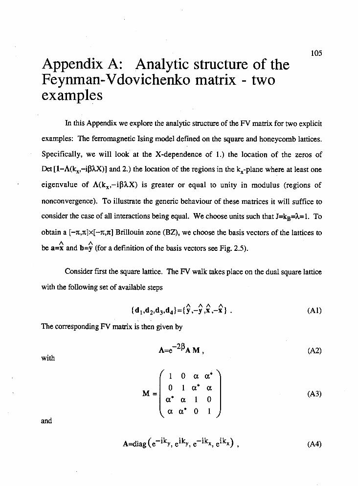
Appendix A: Analytic structure of the Feynman-Vdovichenko matrix - two examples

In this Appendix we explore the analytic structure of the FV matrix for two explicit

examples: The ferromagnetic Ising model defined on the square and honeycomb lattices.

Specifically, we will look at the X-dependence of 1.) the location of the zeros of

Det [1-A(kx,-iphX)] and 2.) the location of the regions in the kx-plane where at least one

eigenvalue of A(kx,-iphX) is greater or equal to unity in modulus (regions of

nonconvergence). To illustrate the generic behaviour of these matrices it will suffice to

consider the case of all interactions being equal. We choose units such that J=kB=h=l. To

obtain a [-IC,IC]X[-x,x] Brillouin zone (BZ), we choose the basis vectors of the lattices to A A

be a=x and b=y (for a definition of the basis vectors see Fig. 2.5).

Consider first the square lattice. The FV walk takes place on the dual square lattice

with the following set of available steps

The corresponding FV matrix is then given by

A = ~ - ~ ~ A M , with

and

1 O a a *

a a * 0 1

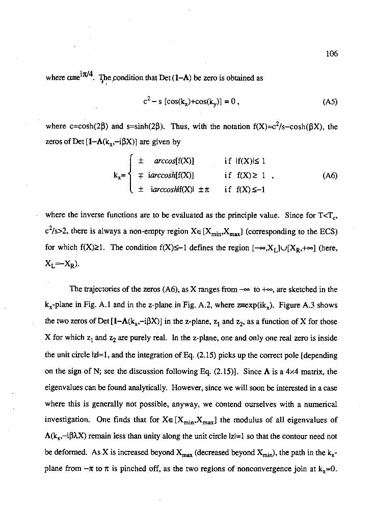
where mix'4. Fe,.condition that Det (1-A) be zero is obtained as I

where c=cosh(2P) and s=sinh(2g). Thus, with the notation f(x)=c2/s-cosh(~~), the

zeros of Det [1-A(kx,-iPX)] are given by

where the inverse functions are to be evaluated as the principle value. Since for TcT,,

c2/s>2, there is always a non-empty region XE [XmI,Xml.] (corresponding to the ECS)

for which f(X)21. The condition f(X)I-1 defines the region [--,X Jv[XR,+-] (here,

X,=-X,).

The trajectories of the zeros (A6), as X ranges from - to +-, are sketched in the

kx-plane in Fig. A.l and in the z-plane in Fig. A.2, where z=exp(ikx). Figure A.3 shows

the two zeros of Det [1-A(kx,-iPX)] in the z-plane, zl and z2, as a function of X for those

X for which zl and q are purely real. In the z-plane, one and only one real zero is inside

the unit circle 1z1=1, and the integration of Eq. (2.15) picks up the correct pole [depending

on the sign of N, see the discussion following Eq. (2.15)]. Since A is a 4x4 matrix, the

eigenvalues can be found analytically. However, since we will soon be interested in a case

where this is generally not possible, anyway, we contend ourselves with a numerical

investigation. One finds that for XE [Xmi,,XmaX] the modulus of all eigenvalues of

A(kx,-iphX) remain less than unity along the unit circle 1z1=1 so that the contour need not

be deformed. As X is increased beyond G, (decreased beyond L), the path in the kx-

plane from -x to x is pinched off, as the two regions of nonconvergence join at kx=O.

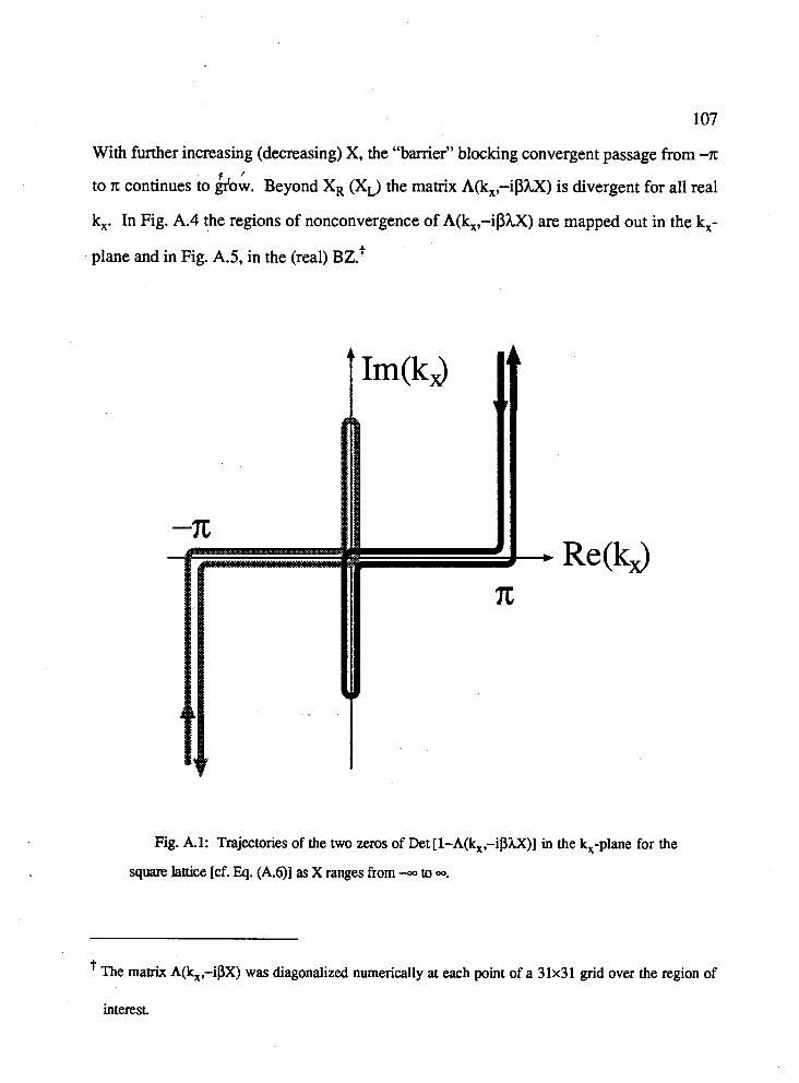
With further increasing (decreasing) X, the "barrier" blocking convergent passage from -n: $ ,'

to n: continues to giow. Beyond XR (XL) the matrix A(kx,-iphX) is divergent for all real

kx. In Fig. A.4 the regions of nonconvergence of A(kx,-iphX) are mapped out in the kx-

plane and in Fig. A S , in the (real) BZ.?

Fig. A.l: Trajectories of the two zeros of Det [1-A(kx,-iphX)] in the kx-plane for the

square lattice [cf. Eq. (Ah)] as X ranges from -.. to 00.

' The matrix A(kx,-ibX) was diagonalized numerically at each paint of a 31x31 grid over the region of

interest.

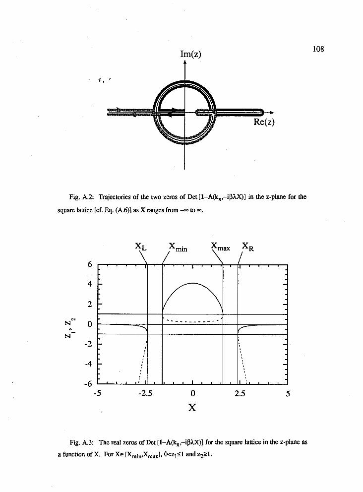
Fig. A.2: Trajectories of the two zeros of Det [1-h(k,,-iphX)] in the z-plane for the

square lattice [cf. Eq. (A.6)] as X ranges from -.. to -.

Fig. A.3: The real zeros of Det [1-A@,,-iphX)] for the square lattice in the z-plane as

a function of X. For XE l & , i n , ~ , ] , Oczlll and z221.

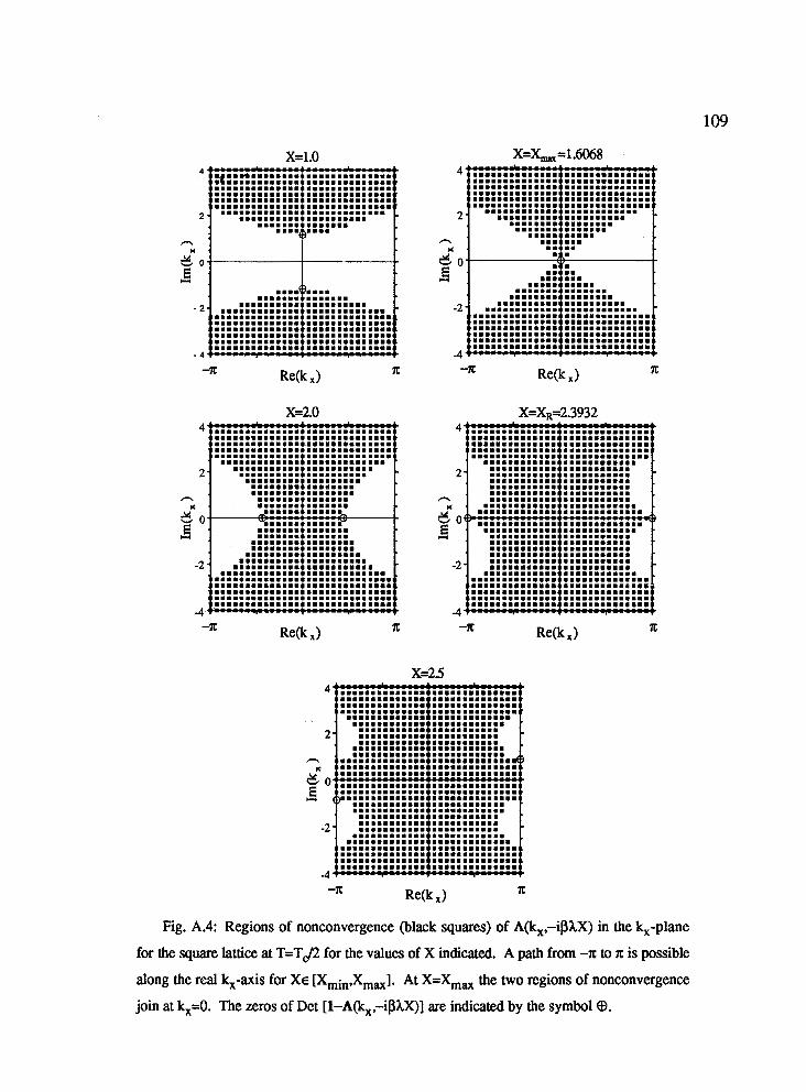
-lC Re& x) X

Fig. A.4: Regions of nonconvergence (black squares) of A@,,-iPXX) in the kx-plane

for the square lattice at T=T$ for the values of X indicated. A path from -x to x is possible

along the real kx-axis for XE [Xmin,Xm,]. At X=Xm, the two regions of nonconvergence

join at kx=O. The zeros of Det [1-A&,-iPXX)] are indicated by the symbol $.

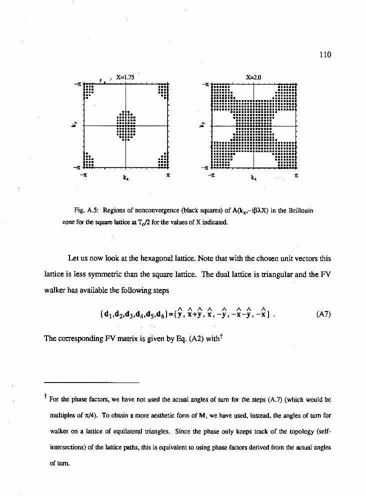
Fig. AS: Regions of nonconvergence (black squares) of A@,,-iphX) in the Brillouin

zone for the square lattice at TJ2 for the values of X indicated.

Let us now look at the hexagonal lattice. Note that with the chosen unit vectors this

lattice is less symmetric than the square lattice. The dual lattice is triangular and the FV

walker has available the following steps

The corresponding FV matrix is given by Eq. (A2) witht

For the phase factors, we have not used the actual angles of turn for the steps (A.7) (which would be

multiples of ~14). To obtain a more aesthetic form of M, we have used, instead, the angles of turn for

walker on a lattice of equilateral triangles. Since the phase only keeps track of the topology (self-

intersections) of the lattice paths, this is equivalent to using phase factors derived from the actual angles

of turn.

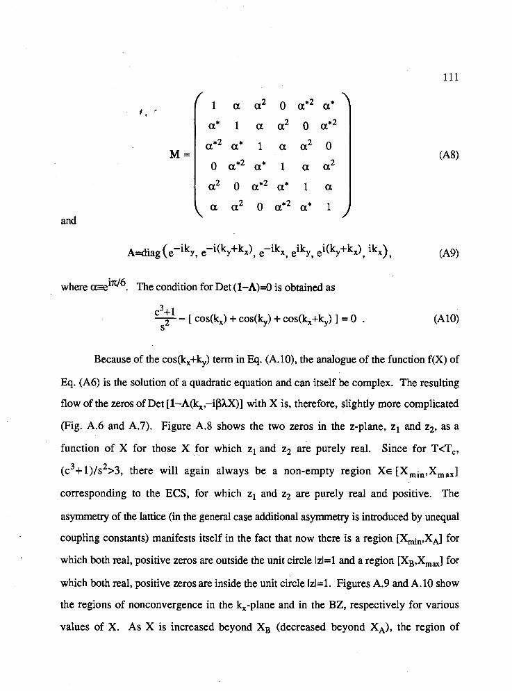
M =

and

ik i(ky+kx) ik,) A=diag(e-iky, e-i(ky+kx), e-ikx, e y, 7 7

where The condition for Det (1-A)=0 is obtained as

Because of the cos(kx+ky) term in Eq. (A.10), the analogue of the function f(X) of

Eq. (A6) is the solution of a quadratic equation and can itself be complex. The resulting

flow of the zeros of Det [1-A(kx,-iphX)] with X is, therefore, slightly more complicated

(Fig. A.6 and A.7). Figure A.8 shows the two zeros in the z-plane, zl and z2, as a

function of X for those X for which zl and z2 are purely real. Since for T<T,,

(c3+l)/s2>3, there will again always be a non-empty region XE [Xmin,Xm,,]

corresponding to the ECS, for which zl and z2 are purely real and positive. The

asymmetry of the lattice (in the general case additional asymmetry is introduced by unequal

coupling constants) manifests itself in the fact that now there is a region [Xmin,XA] for

which both real, positive zeros are outside the unit circle lzl= 1 and a region [XB,Xmax] for

which both real, positive zeros are inside the unit circle M=1. Figures A.9 and A.10 show

the regions of nonconvergence in the k,-plane and in the BZ, respectively for various

values of X. As X is increased beyond XB (decreased beyond XA), the region of

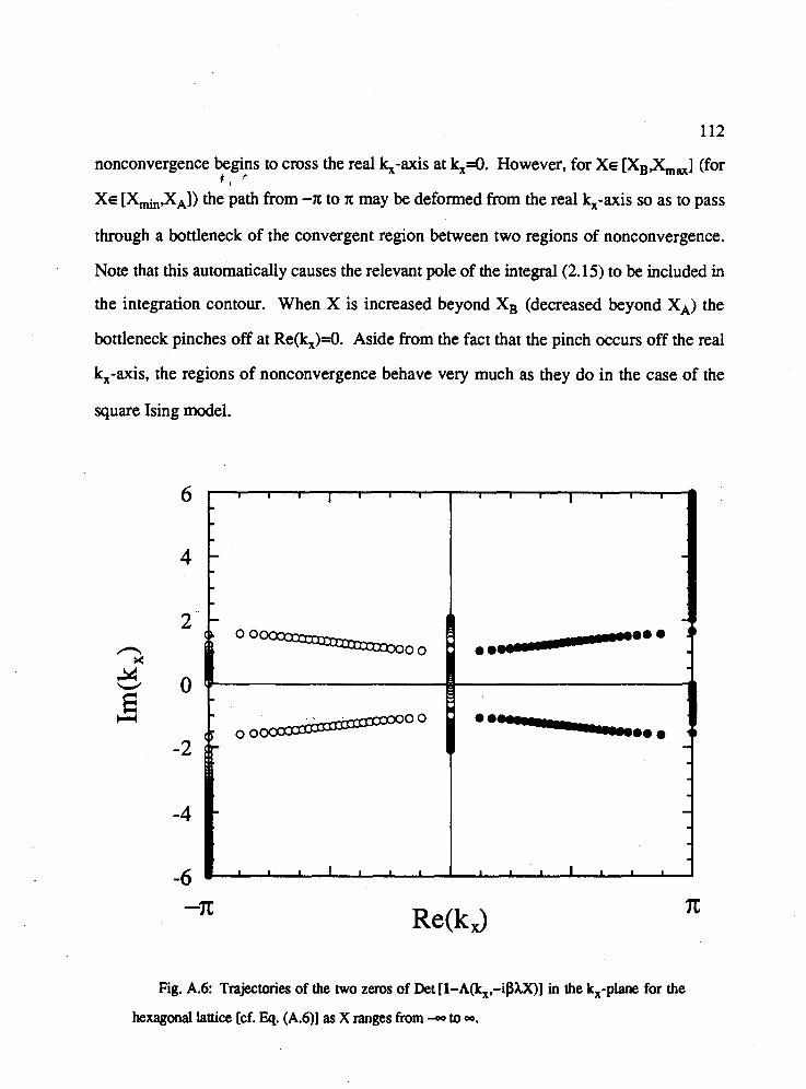
112

nonconvergence begins to cross the real kx-axis at kx=O. However, for XE [ X B A B x ] (for + , '

XE [Xmin,XA]) the path from -x to x may be deformed from the real k,-axis so as to pass

through a bottleneck of the convergent region between two regions of nonconvergence.

Note that this automatically causes the relevant pole of the integral (2.15) to be included in

the integration contour. When X is increased beyond XB (decreased beyond XA) the

bottleneck pinches off at Re(kx)=O. Aside from the fact that the pinch occurs off the real

kx-axis, the regions of nonconvergence behave very much as they do in the case of the

square Ising model.

Fig. A.6: Trajectories of the two zeros of Det [1-A@,,-$AX)] in the kx-plane for the

hexagonal lattice [cf. Eq. (A.6)] as X ranges from -O to -.

Fig. A.7: Trajectories of the two zeros of Det [1-A@,,-iP5X)I in the z-plane for the

hexagonal lattice [cf. Eq. (A.6)1 as X ranges from -oo to -. The circle shown (thin solid line)

is the unit circle M=1. The trajectories off the real axis become increasingly heart-shaped as

Fig. A.8: The real zeros of Det [1-A&,-i$XX)] in the z-plane for the hexagonal

lattice as a function of X. For XE [ X A , X B ] , O<zlSl and 2221. For

XE [Xmin,XA]~[XB,Xmax], either both or neither positive zeros are inside the unit circle

1z1= 1.

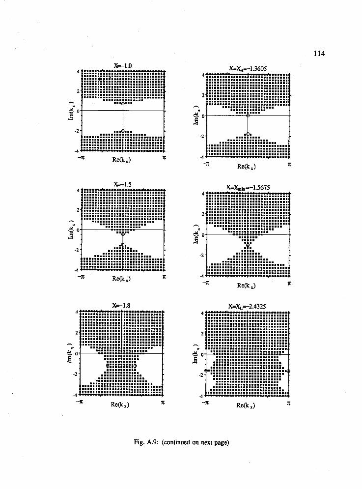
.I. L.. .......... .............. .................... ............................ -'b/ ..m....mmmm...m............. .....................m...... ............................ -4

Fig. A.9: (continued on next page)

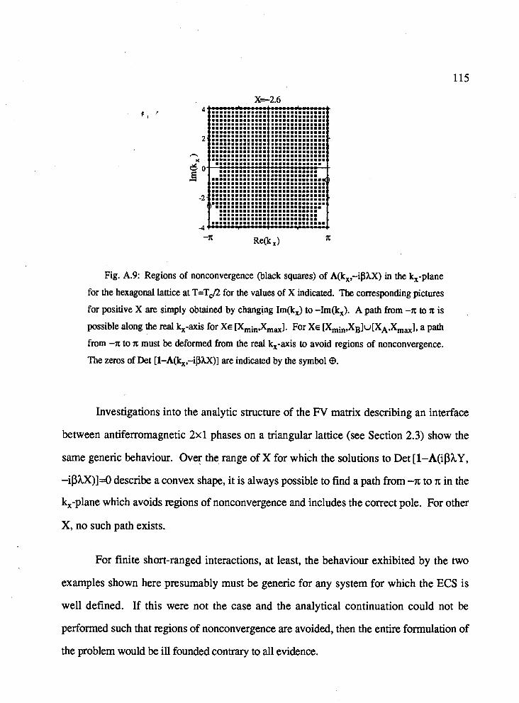
Fig. A.9: Regions of nonconvergence (black squares) of A(k,,-@AX) in the kx-plane

for the hexagonal lattice at T=T$ for the values of X indicated. The corresponding pictures

for positive X are simply obtained by changing Im(k,) to -Im(kx). A path from -A to 7c is

possible along the real kx-axis for XE [Xmin,Xmax]. For XE [Xmin,XB]~[XA,Xmax], a path

from -x to x must be deformed from the real kx-axis to avoid regions of nonconvergence.

The zeros of Det [1-A(k,,-iPXX)] are indicated by the symbol $.

Investigations into the analytic structure of the FV matrix describing an interface

between antiferromagnetic 2x1 phases on a triangular lattice (see Section 2.3) show the

same generic behaviour. Over the range of X for which the solutions to Det [1-A(iphY,

-iPkX)]=O describe a convex shape, it is always possible to find a path from -n: to n: in the

kx-plane which avoids regions of nonconvergence and includes the correct pole. For other

X, no such path exists.

For finite short-ranged interactions, at least, the behaviour exhibited by the two

examples shown here presumably must be generic for any system for which the ECS is

well defined. If this were not the case and the analytical continuation could not be

performed such that regions of nonconvergence are avoided, then the entire formulation of

the problem would be ill founded contrary to all evidence.

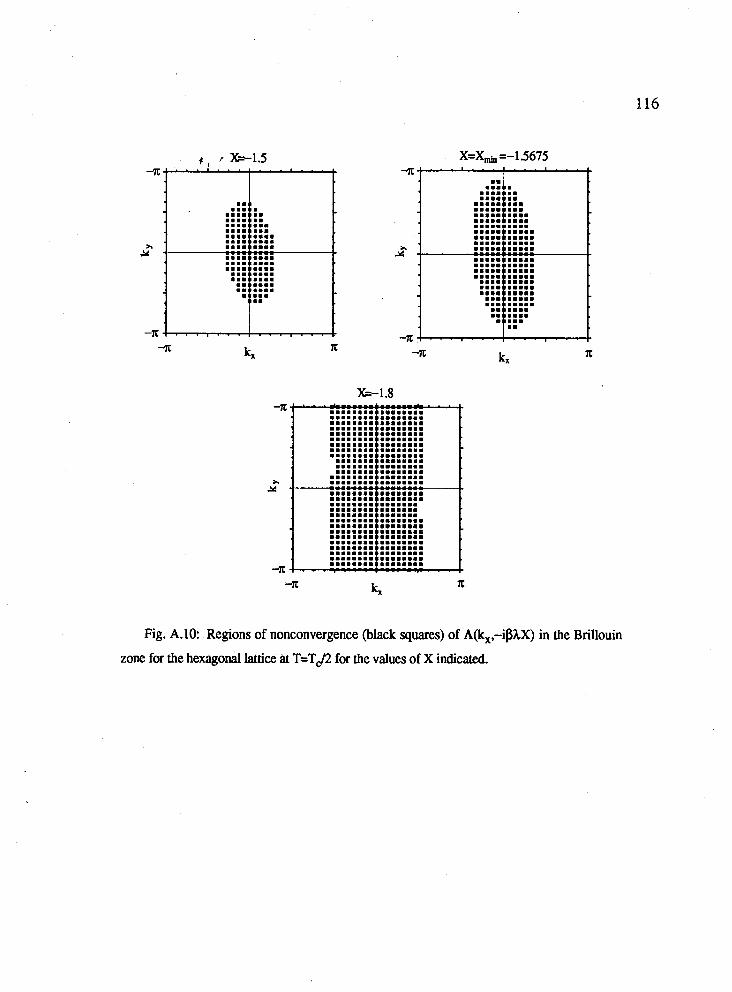
Fig. A.lO: .Regions of nonconvergence (black squares) of A(k,,-iphX) in the Brillouin

zone for the hexagonal lattice at T=T$ for the values of X indicated.

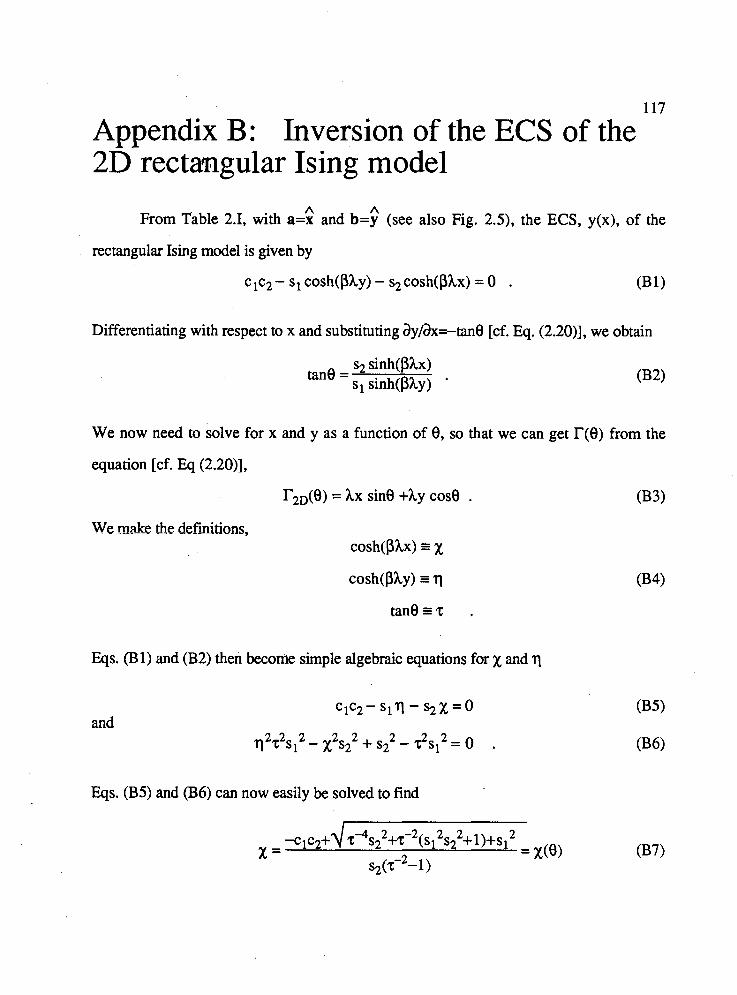
117

Appendix B: Inversion of the ECS of the 2D rectangular Ising model

A A From Table 2.1, with a=x and b=y (see also Fig. 2.5), the ECS, y(x), of the

rectangular Ising model is given by

Differentiating with respect to x and substituting ay/ax=-tan0 [cf. Eq. (2.20)], we obtain

We now need to solve for x and y as a function of 0, so that we can get r(0) from the

equation [cf. Eq (2.20)],

r2&3) = hx sine +hy c o d . 033)

Eqs. (I3 1) and (B2) then become simple algebraic equations for x and q

C1C2- s l q - s2x = o and

q2Z2sI2 - X2sZ2 + s22 - 3 s l 2 = 0 .

Eqs. (B5) and (B6) can now easily be solved to find

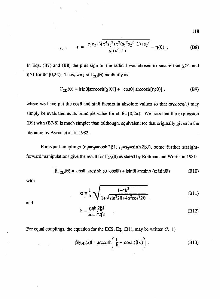
In Eqs. (B7) arid (B8) the plus sign on the radical was chosen to ensure that 221 and

q 2 l for 8~ [0,27t). Thus, we get r2D(0) explicitly as

where we have put the cos0 and sin0 factors in absolute values so that arccosh(.) may

simply be evaluated as its principle value for all 0~ [0,2n). We note that the expression

(B9) with (B7-8) is much simpler than (although, equivalent to) that originally given in the

literature by Avron et al. in 1982.

For equal couplings (cl=c2=cosh 2PJ; sl =s2=sin h 2PJ), some further straight-

forward manipulations give the result for r2&) as stated by Rottman and Wortis in 1981:

Pr2D(0) = lcos0l arcsinh (a Icosel) + Isinel arcsinh ( a Isinel) (B 10)

with

and - sinh 2PJ h =

c o s h 2 2 ~ ~

For equal couplings, the equation for the ECS, Eq. (B I), may be written (h=l)

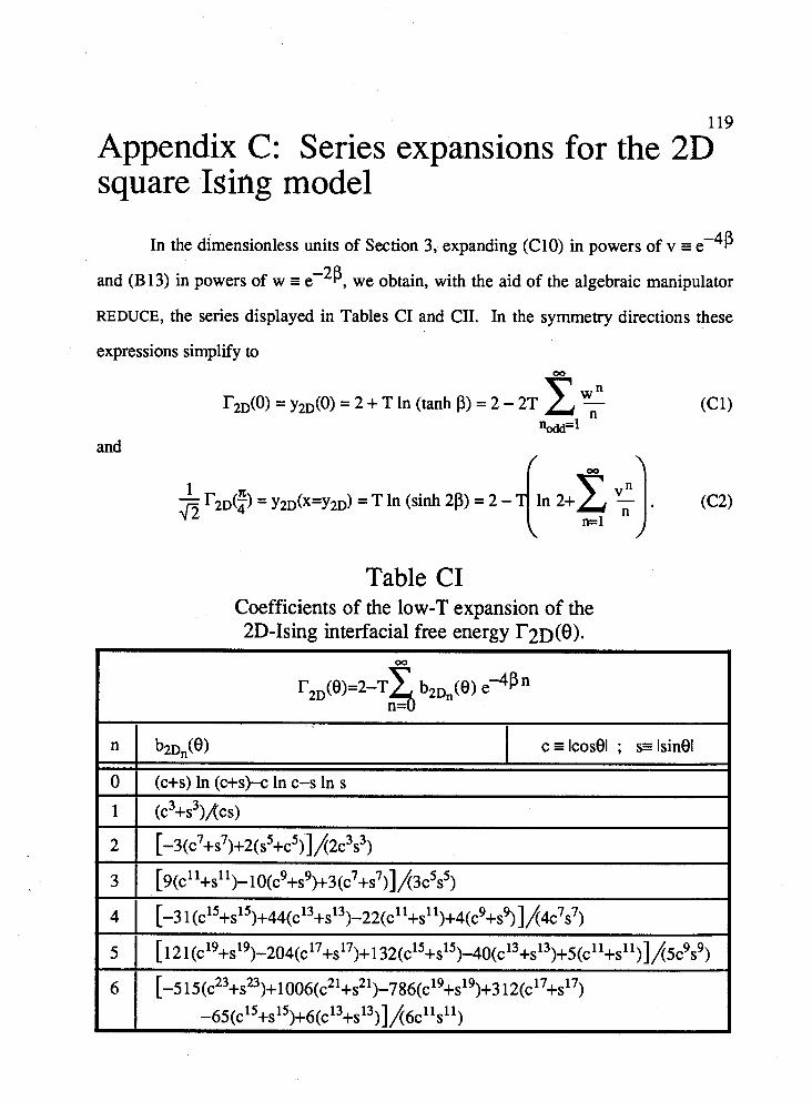
Appendix C: Series expansions for the 2D square Ising model

In the dimensionless units of Section 3, expanding (C10) in powers of v I e -4P -

and (Bl3) in powers of w = e 2P, we obtain, with the aid of the algebraic manipulator

REDUCE, the series displayed in Tables CI and CII. In the symmetry directions these

expressions simplify to

and

Table CI Coefficients of the low-T expansion of the 2D-Ising interfacial free energy r 2 ~ ( 8 ) .

b2~,(9) c I ~cose~ ; s= Isinel

0 1 (c+s) In (c+s)-c In c-s In s

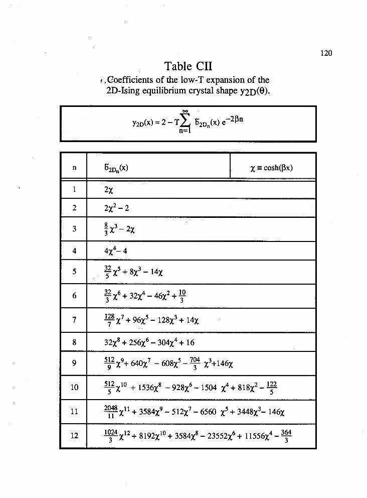
Table CII 4 , Coefficients of the low-T expansion of the

2D-Ising equilibrium crystal shape y 2 ~ ( 8 ) .

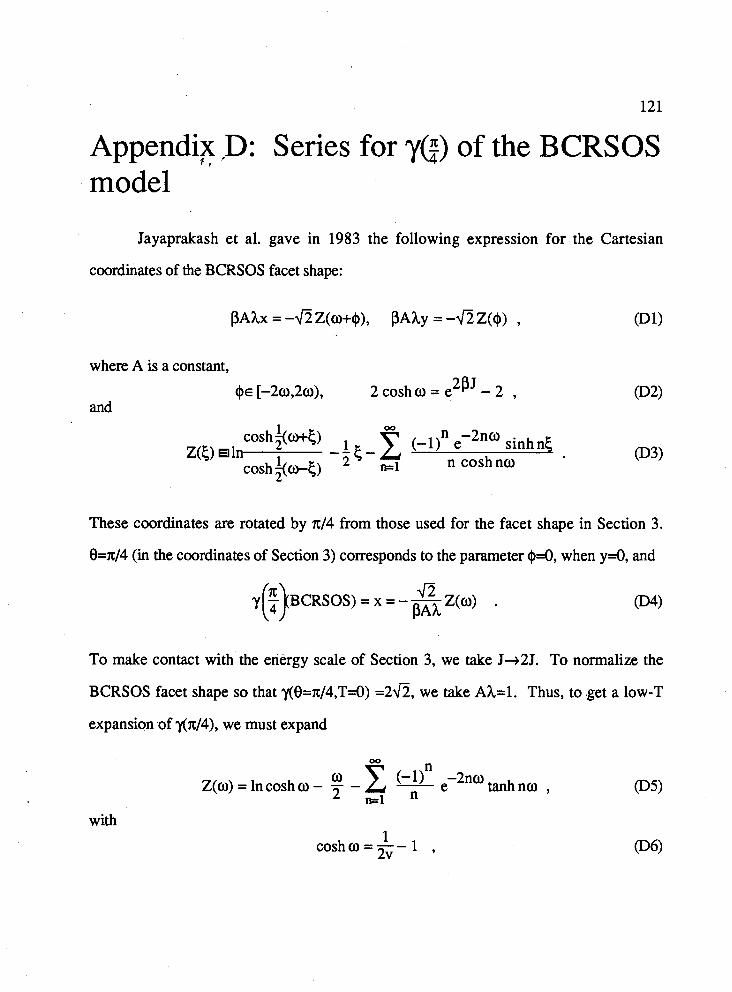
Appendix f , D: Series for y(f) of the BCRSOS model

Jayaprakash et al. gave in 1983 the following expression for the Cartesian

coordinates of the BCRSOS facet shape:

where A is a constant,

(PE WWW, 2 cosh o = e2pJ - 2 , and

@2)

00

cosh $w+Q Z({) In

cosh %a-c) n=1 n coshno @3)

These coordinates are rotated by ~ 1 4 from those used for the facet shape in Section 3.

8-14 (in the coordinates of Section 3) corresponds to the parameter $4, when y=O, and

To make contact with the enQgy scale of Section 3, we take J+2J. To normalize the

BCRSOS facet shape so that y(9=7c/4,T=O) =2*, we take Ah=l. Thus, to get a low-T

expansion of y(~/4), we must expand

with 1

cosho = -- 2v 1 ,

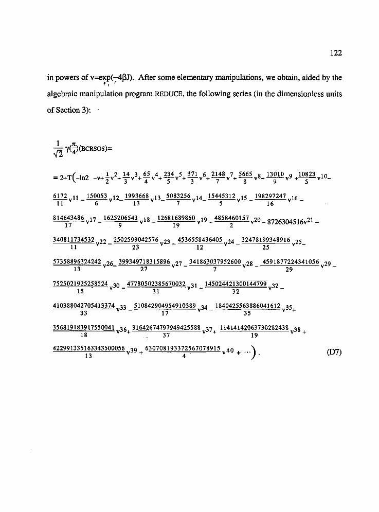
in powers of v=exp(4PJ). After some elementary manipulations, we obtain, aided by the 4 , '

algebraic manipulation program REDUCE, the following series (in the dimensionless units

of Section 3): .

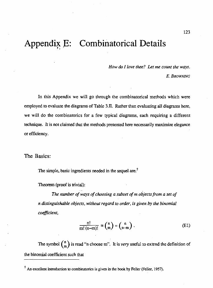
Appendix E: Combinatorical Details C ,

How do I love thee? Let me count the ways.

E. BROWNING

In this Appendix we will go through the combinatorical methods which were

employed to evaluate the diagrams of Table 3.n. Rather than evaluating all diagrams here,

we will do the combinatorics for a few typical diagrams, each requiring a different

technique. It is not claimed that the methods presented here necessarily maximize elegance

or efficiency.

The Basics:

The simple, basic ingredients needed in the sequel are:?

Theorem (proof is trivial):

The number of ways of choosing a subset of m 06jectsfrom a set of

n distinguishable objects, without regard to order, is given by the binomial

co@cient,

n ! m! (n-m)!

The symbol (:) is read "n choose m". It is very useful to extend the definition of

the binomial coefficient such that

An excellent introduction to combinatorics is given in the book by Feller (Feller. 1957).

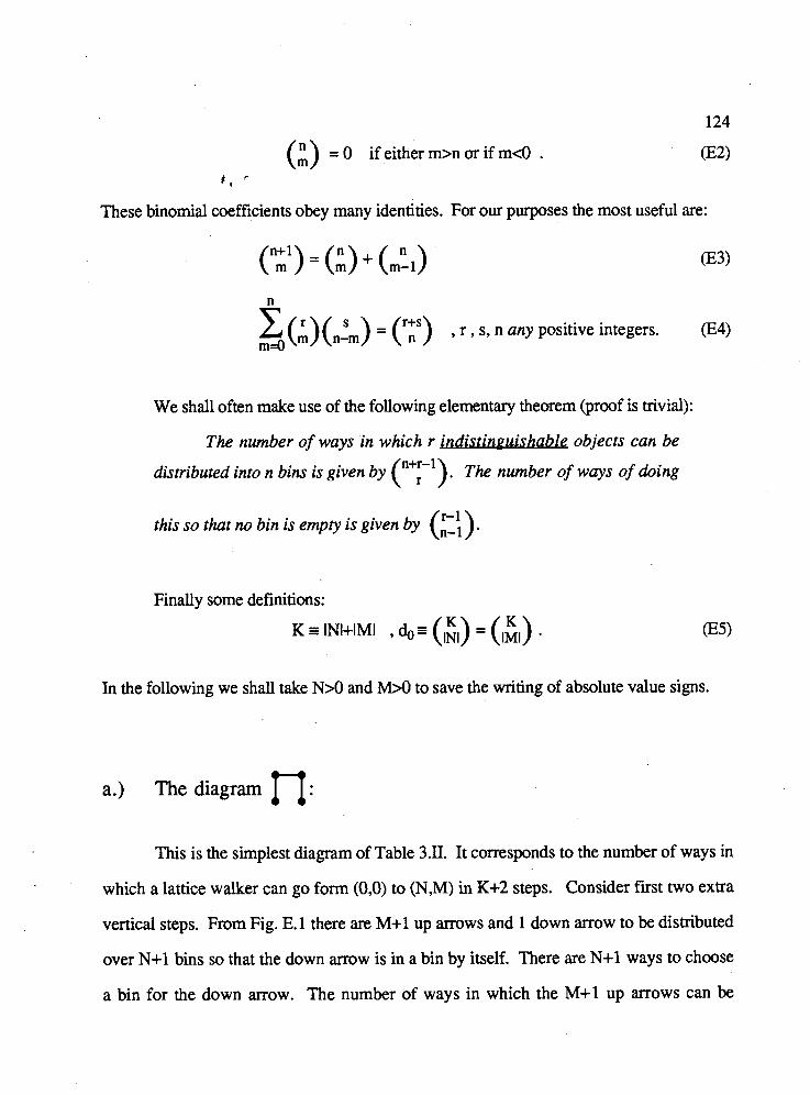
124

(i) = 0 if either mm or if m<0 . @2) + r

These binomial coefficients obey many identities. For our purposes the most useful are:

n

C (i)(nk) = (r;;s) , r , s, n any positive integers. m 4

034)

We shall often make use of the following elementary theorem (proof is trivial): . . . The number of ways in which r m d l s t r n ~ u a b l e objects can be

n+r-1 distributed into n bins is given by ( ). The number of ways of doing

this so that no bin is empty is given by (:I:).

Finally some definitions:

In the following we shall take N>O and M>O to save the writing of absolute value signs.

a.) Thediagram n: This is the simplest diagram of Table 3.n. It corresponds to the number of ways in

which a lattice walker can go form (0,O) to (N,M) in K+2 steps. Consider first two extra

vertical steps. From Fig. E. 1 there are M+l up arrows and 1 down arrow to be distributed

over N+l bins so that the down arrow is in a bin by itself. There are N+l ways to choose

a bin for the down arrow. The number of ways in which the M+l up arrows can be

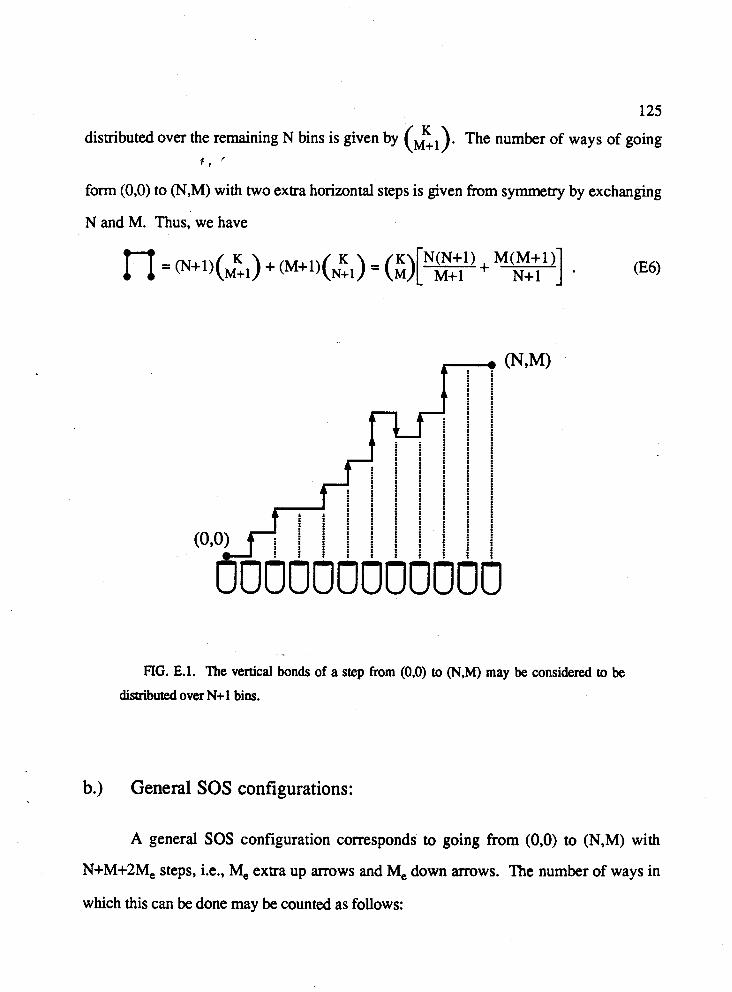
125

distributed over the remaining N bins is given by (GI). The number of ways of going + , '

form (0,O) to (N,M) with two extra horizontal steps is given from symmetry by exchanging

N and M. Thus, we have

FIG. E.1. The vertical bonds of a step from (0,O) to (N,M) may be considered to be

dism'buted over N+l bins.

b.) General SOS configurations:

A general SOS configuration corresponds to going from (0,O) to (N,M) with

N+M+2Me steps, i.e., Me extra up arrows and Me down arrows. The number of ways in

which this can be done may be counted as follows:

Choose 1 put of the N+l available bins. There are (N;l)=~+ 1 ways of doing

this. Put all down arrows into that bin. There are (?=')=I ways of doing that.

Distribute the M+Me up arrows over the (N+l)-1 remaining bins. There are (N+l)- l+M+Me- 1 ) ways of doing that.

Choose 2 of the N+l bins. There are ways of doing this. Put all down

arrows into the 2 bins so that there is at least one down arrow in each of the 2 bins (the

case where one of the 2 bins is empty has been counted already). There are ( y 2 ) Ways

of doing that. Distribute the M+Me up arrows over the (N+l)-2 remaining bins. There are (N+ 1 )-2+M+Me- 1 ) ways of doing that.

Keep doing this until all possibilities of distributing down arrows into bins are

exhausted: If w2N, the process of the previous steps must stop after N bins have been

chosen for down arrows. (One bin must be left for up arrows.) If Me<N, the process

stops after M, bins have been chosen for the down arrows.

Summing over the possibilities of distributing down arrows we get that the number

of distinct SOS configurations is given by

min Me,N) 8 (Y ) (z') (:>;) .

At first sight one might worry about the min(.) function in the upper limit of the

summation. However, the property (E2) of the binomial coefficients ensures that the

summation is cut off correctly, whether we take the upper limit to be N or Me.

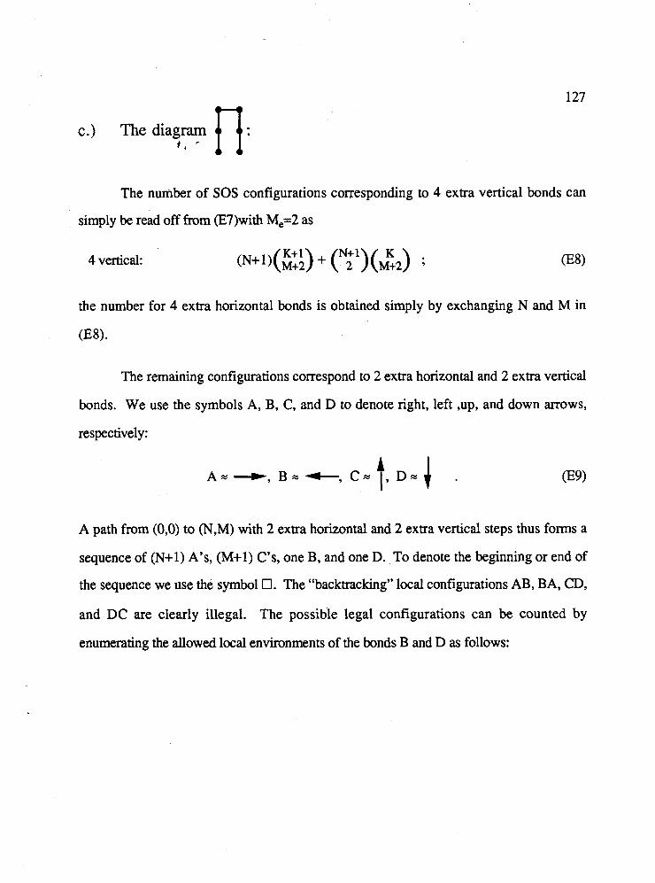
c.) The diagram C , *

The number of SOS configurations corresponding to 4 extra vertical bonds can

simply be read off from (E7)with M,=2 as

4 vertical:

the number for 4 extra horizontal bonds is obtained simply by exchanging N and M in

(W.

The remaining configurations correspond to 2 extra horizontal and 2 extra vertical

bonds. We use the symbols A, B, C, and D to denote right, left ,up, and down arrows,

respectively:

A path from (0,O) to (N,M) with 2 extra horizontal and 2 extra vertical steps thus forms a

sequence of (N+l) A's, (M+l) C's, one B, and one D. To denote the beginning or end of

the sequence we use the syrnbl 0. The "backtracking" local configurations AB, BA, CD,

and DC are clearly illegal. The possible legal configurations can be counted by

enumerating the allowed local environments of the bonds B and D as follows:

Table E.1 The pessible configurations of a path from (0,O) to (N,M)

with two extra vertical bonds and two extra horizontal bonds without immediate backtracking

[1I

[2]

[3]

[4]

[5]

[6]

In this Table, "2~" indicates that for every sequence (configuration) containing the

[7]

given local configuration(s), 'another configuration can be obtained by ordering the

1m-d configuration(s)

CBC ADA

2x ADBC

2x ODA CBC

2x OBC ADA

2x OBDA

2x ODBC

sequence in reverse.

2x OBC ADO

Not all configurations counted in Table E.1 belong to the diagram , however.

Some configurations belong to the diagram ; others correspond to self-

# of A's left over

N-1

N

N

N-1

N

N+l

intersections. For each of the rows of Table E.1, these additional illegal configurations are:

N

# of B's lefr over

M-l

M

M-1

M

M+l

M

# of compatible configurations

(N+M) ! (N-l)!(M-I)!

= 4 N M

(N+M+ 1) ! N! M! = 2&(K+1)

(N+M) ! N! (M-l)! = 2 4 M

(N+M) ! (N-I)! M! = 2 4 N

(N+M+ I)! K+ 1 N! (M+l)! = 2 d 0 ~ + 1

(N+M+ I)! K+ 1 (N+l)! M! = 2 4 ~

M (N+M) ! N! M! = 2 4

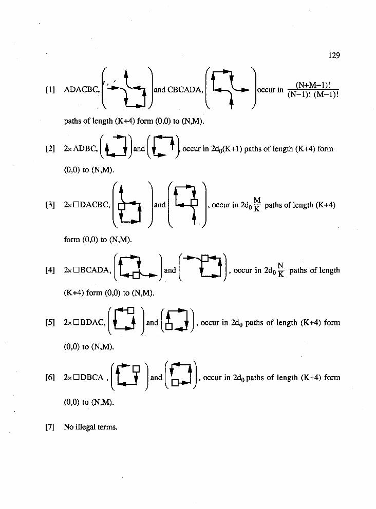
1 1 -AcBc, [+land cBCmA, [L+] occur in (N-I)! (N+M-l)! (M-I)!

paths of length (K+4) form (0,O) to (N,M).

[2] 2x ADBC, [d) and [ p) occur in 2&(K+l) paths of length (K+4) form

M [3] 2x ClDACBc, [b land [q.], occur in 2& paths of length &+4)

form (0,O) to (N,M).

[4] 2x OBCADA, N (a) and (m) . r,cw in 2dn pihs ri length

&+4) form (0,O) to (N,M).

[I] 2x El BDAC, [E ) and (a) , occur in ido paths of length ( K A ) form

[61 2, UDBCA , [u ) and [a), occur in 2 4 paths of length (K+4) form

[7] No illegal terms.

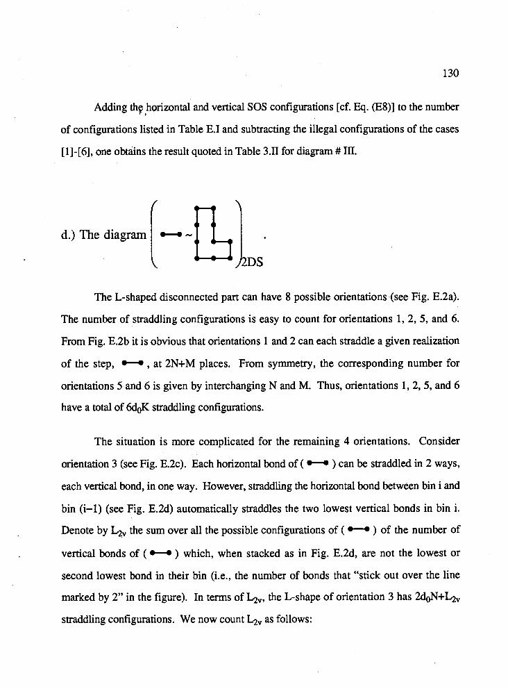
Adding the horizontal and vertical SOS configurations [cf. Eq. (B)] to the number I

of configurations listed in Table E.1 and subtracting the illegal configurations of the cases

[I]-[6], one obtriins the result quoted in Table 3.II for diagram # III.

d.) The diagram

The L-shaped disconnected part can have 8 possible orientations (see Fig. E.2a).

The number of straddling configurations is easy to count for orientations 1, 2, 5, and 6.

From Fig. E.2b it is obvious that orientations 1 and 2 can each straddle a given realization

of the step, - , at 2N+M places. From symmetry, the corresponding number for

orientations 5 and 6 is given by interchanging N and M. Thus, orientations 1,2,5, and 6

have a total of 6d& straddling configurations.

The situation is more complicated for the remaining 4 orientations. Consider

orientation 3 (see Fig. E.2c). Each horizontal bond of ( - ) can be straddled in 2 ways,

each vertical bond, in one way. However, straddling the horizontal bond between bin i and

bin (i-1) (see Fig. E.2d) automatically straddles the two lowest vertical bonds in bin i.

Denote by LQ, the sum over all the possible configurations of ( O-O ) of the number of

vertical bonds of ( - ) which, when stacked as in Fig. E.2d, are not the lowest or

second lowest bond in their bin (i.e., the number of bonds that "stick out over the line

marked by 2" in the figure). In terms of b , , the L-shape of orientation 3 has 2doN+L2,

straddling configurations. We now count La as follows:

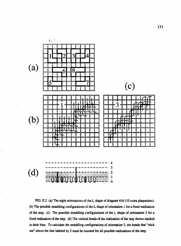
FIG. E.2 (a) The eight orientations of the L shape of diagram #16 (10 extra plaquettets).

(b) The possible straddling configurations of the L shape of orientation 1 for a fixed realization

of the step. (c) The possible straddling configurations of the L shape of orientation 3 for a

fixed realization of the step. (d) The vertical bonds of the realization of the step shown stacked

in their bins. To calculate the straddling configurations of orientation 3, the bonds Uat "stick

outn above the line labeled by 2 must be counted for all possible realizations of the step.

Choose i of the N+l bins. There are (N:l) ways of doing that. C , '

Put one vertical bond into each of the i bins.

choose j of the i bins just selected. There are 0 ways of doing that.

Fill these j bins with the M-i remaining vertical bonds so that none of the j

M-i- 1 bins has less than (a total of) 2 vertical bonds. There are ( j-l ) ways of

doing that.

There are now M-i-j vertical bonds sticking out above the line at height 2.

Sum over j until all i bins are exhausted.?

Sum over i until all (N+l) bins are used.?

Thus, we get

L2" =

N+ 1

= (":I)$ (I) (";I) (M-i-j) + (end effect) = Q(N,M) + (end effect), (EIO)

where (end effect) refers to the number of ways in which vertical bonds on the first bin can

be straddled that are not included in b,. Since the first bin is not preceded by a vertical

bond, the two lowest vertical bonds in the first bin (if there are any) can never be

automatically straddled by an L straddling the nonexistent preceding horizontal bond. The

end effect is, therefore, given by

' Again, we need not worry about running out of bonds before running out of bins because of property

(W.

(end effect) = (number of configurations with exactly one bond in the first bin) + 2x , (npmber of configurations with at least 2 vertical bonds in the first bin) .

I

If there is exactly 1 bond in bin 1, then the following horizontal bond always ends at

position (1,l). Thus, the number of configurations with exactly one bond in the first bin is

simply given by the number of ways in which one can get from (1,l) to (N,M) with

N+M-2 steps. Likewise, if we are guarantied that there are at least 2 bonds in bin 1, the

remaining part of ( O-O ) is tethered at (0,2) and (N,M). The number of configurations

with at least 2 vertical bonds in the first bin is, therefore, given by the number of ways in

which one can go from (0,2) to (N,M) in N+M-2 steps. We obtain

NM+2[M(M-I)] (end effect) = (:I:) + 2(Ki2) = & K(K-l) (El 1)

The double sum R(N,M) is evaluated straightforwardly via repeated application of

identity (E4). The only new kind of sum that occurs is of the form

This sum is easily evaluated by writing

j (!) = j i! - i (i-I)! = i c-;) j! (i-j)! - 0-I)! (i-j)! -

Substituting (E13) into (E12) we get

where the last equality follows immediately from identity (E4). After a little algebra of this

sort one gets

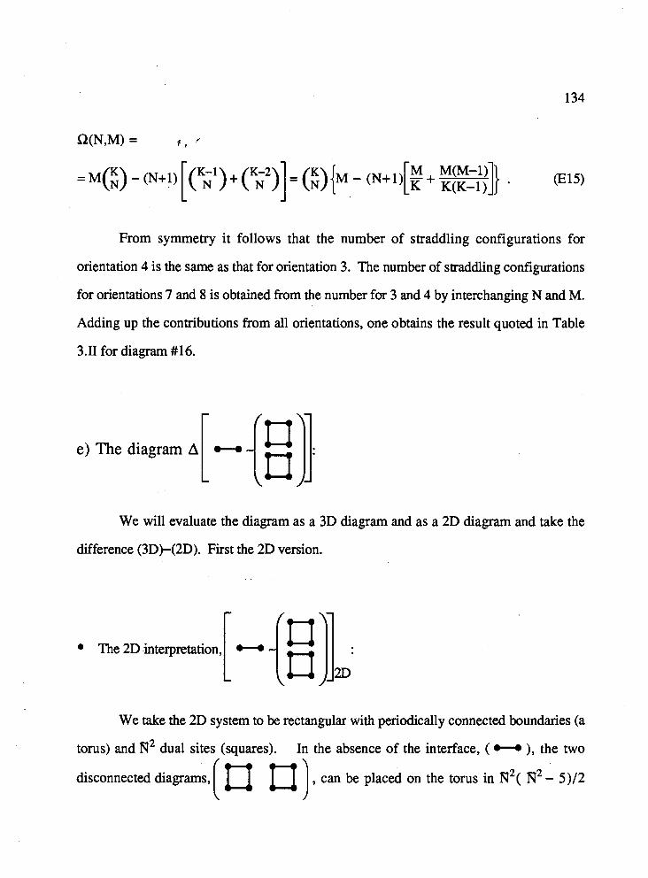
From symmetry it follows that the number of straddling configurations for

orientation 4 is the same as that for orientation 3. The number of straddling configurations

for orientations 7 and 8 is obtained from the number for 3 and 4 by interchanging N and M.

Adding up the contributions from all orientations, one obtains the result quoted in Table

3.11 for diagram #16.

We will evaluate the diagram as a 3D diagram and as a 2D diagram and take the

difference (3D)-(2D). First the 2D version.

We take the 2D system to be rectangular with periodically connected boundaries (a

torus) and fi12 dual sites (squares). In the absence of the interface, ( ), the two

disconnected diagrams, , can be placed on the torus in fi12( FJ2 - 5 ) / 2

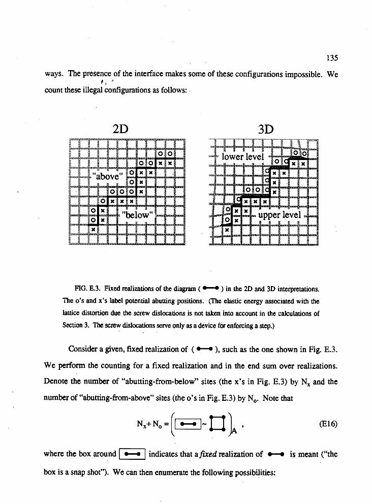
ways. The presence of the interface makes some of these configurations impossible. We + , .

count these illegal configurations as follows:

FIG. E.3. Fixed realizations of the diagram ( - ) in the 2D and 3D interpretations.

The 0's and x's label potential abutting positions. (The elastic energy associated with the

lattice distortion due the screw dislocations is not taken into account in the calculations of

Section 3. The screw dislocations serve only as a device for enforcing a step.)

Consider a given, fixed realization of ( - ), such as the one shown in Fig. E.3.

We perform the counting for a fixed realization and in the end sum over realizations.

Denote the number of "abutting-from-below" sites (the x's in Fig. E.3) by N, and the

number of "abutting-from-above" sites (the 0's in Fig. E.3) by No. Note that

where the box around indicates that a f i ed realization of c-. is meant ("the

box is a snap shot"). We can then enumerate the following possibilities:

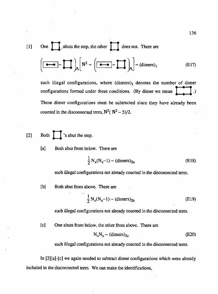
[I] One f7 abuts the step, the other n does not. There are

such illegal configurations, where (d imer~)~ denotes the number of dimer

configurations formed under these conditions. (By dimer we mean 1-1 .)

These dimer configurations must be subtracted since they have already been

counted in the disconnected term, m2( F12 - 5)/2.

[2] Both U 's abut the step.

[a] Both abut from below. There are

i - N,(Nx-1) - (dimer~)~, 2 @W

such illegal configurations not already counted in the disconnected term.

[b] Both abut from above. There are

such illegal configurations not already counted in the disconnected term.

[c] One abuts from below, the other from above. There are

NoNx - (dimer~)~, (Em

such illegal configurations not already counted in the disconnected term.

In [2][a]-[c] we again needed to subtract dimer configurations which were already

included in the disconnected term. We can make the identifications,

and

Subtracting from the disconnected part the illegal contributions from [I] and [2], we

finally obtain

The {:]I :

3D

We assume the 2D interface to be toroidally connected and to have N2 plaquettes

(see also the discussion in Section 3.3). In the absence of a step there are N2( N~ - 5112

ways of having two desorptions , as many ways to have two adsorptions

, and m2( N2 - 1) ways of having both an adsorption and a desorption

giving a net disconnected contribution of 2N2(m2-3). We must now count which of these

configurations are not possible in the presence of a step, *--a . Again, we consider a

fixed realization of the step. Recall that desorptions are allowed to abut the step on the

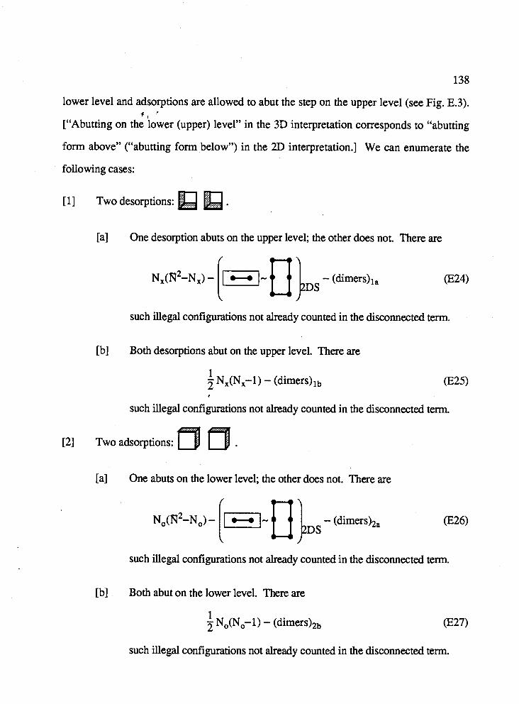
lower level and adsorptions are allowed to abut the step on the upper level (see Fig. E.3). + , -

["Abutting on the lower (upper) level" in the 3D interpretation corresponds to "abutting

form above" ("abutting form below") in the 2D interpretation.] We can enumerate the

following cases:

3 /"gm f [I] Two desorptions: ..,, ,,, .

[a] One desorption abuts on the upper level; the other does not. There are

(E24)

such illegal configurations not already counted in the disconnected term.

[b] Both desorptions abut on the upper level. There are

*

such illegal configurations not already counted in the disconnected term.

[2] Two adsorptions: ..

[a] One abuts on the lower level; the other does not. There are

such illegal configurations not already counted in the disconnected term.

[b] Both abut on the lower level. There are

1 - No(No-1) - ( d i m e r ~ ) ~ ~ 2 ($27)

such illegal configurations not already counted in the disconnected term.

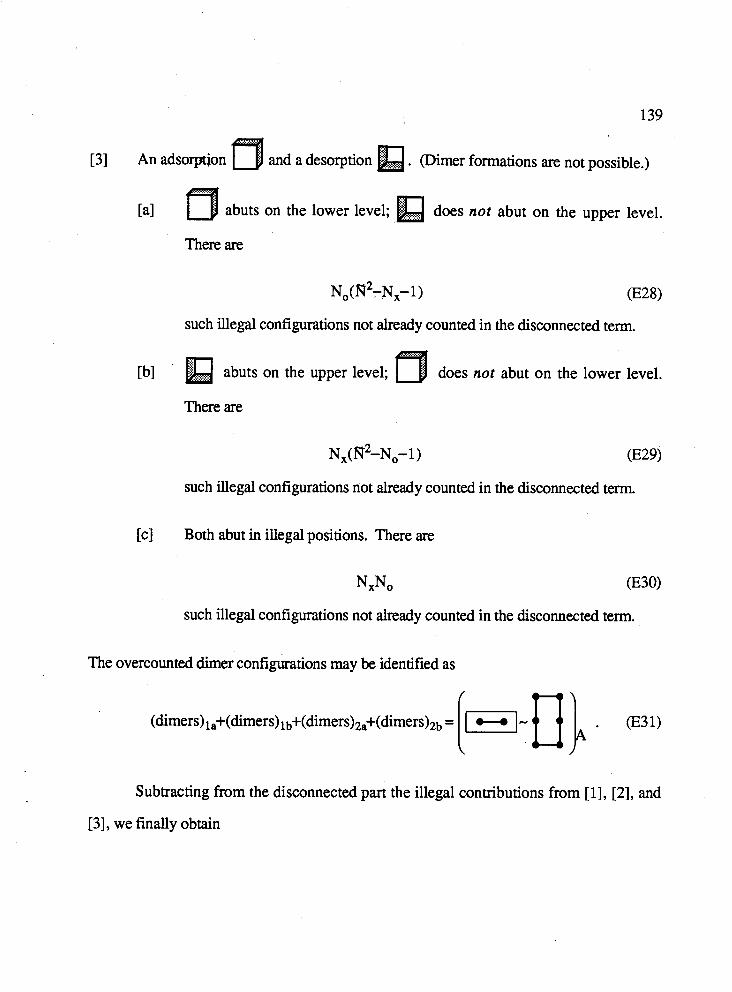
[3] An adsorption and a desorption . (Dimer formations are not possible.)

[a] abuts on the lower level; does not abut on the upper level.

There are

such illegal configurations not already counted in the disconnected term.

[b] a abuts on the upper level; does nor abut on the lower level.

There are

NJN~-N,-I 0329)

such illegal configurations not already counted in the disconnected term.

icj Both abut in illegal positions. There are

NXNO @30)

such illegal configurations not already counted in the disconnected term.

The overcounted dirner configurations may be identified as

Subtracting from the disconnected part the illegal contributions from [I], [2], and

[3], we finally obtain

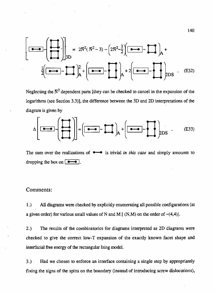
Neglecting the N2 dependent parts [they can be checked to cancel in the expansion of the

logarithms (see Section 3.3)], the difference between the 3D and 2D interpretations of the

diagram is given by

The sum over the realizations of is trivial in this case and simply amounts to

dropping the box on 1-1.

Comments:

1 .) All diagrams were checked by explicitly enumerating all possible configurations (at

a given order) for various small values of N and M [ (N,M) on the order of -(4,4)].

2.) The results of the combinatorics for diagrams interpreted as 2D diagrams were

checked to give the correct low-T expansion of the exactly known facet shape and

interfacial free energy of the rectangular Ising model.

3.) Had we chosen to enforce an interface containing a single step by appropriately

fixing the signs of the spins on the boundary (instead of introducing screw dislocations),

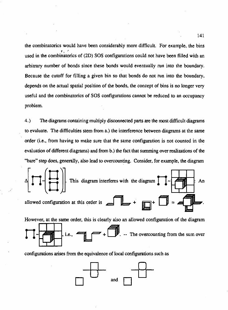
the combinatorics would have been considerably more difficult. For example, the bins + , '

used in the combinatorics of (2D) SOS configurations could not have been filled with an

arbitrary number of bonds since these bonds would eventually run into the boundary.

Because the cutoff for filling a given bin so that bonds do not run into the boundary,

depends on the actual spatial position of the bonds, the concept of bins is no longer very

useful and the combinatorics of SOS configurations cannot be reduced to an occupancy

problem.

4.) The diagrams containing multiply disconnected parts are the most difficult diagrams

to evaluate. The difficulties stem from a.) the interference between diagrams at the same

order (i.e., from having to make sure that the same configuration is not counted in the

evaluation of different diagrams) and from b.) the fact that summing over realizations of the

"bare" step does, generally, also lead to overcounting. Consider, for example, the diagram

{dl] This diagram interferes with the diagram

,"

. . . . . . . allowed configuration at this order is fi + + 0 =

However, at the same order, this is clearly also an allowed configuration of the diagram ...... . . . ... .........

. -- The overcounting from the sum over

configurations arises from the equivalence of local configurations such as

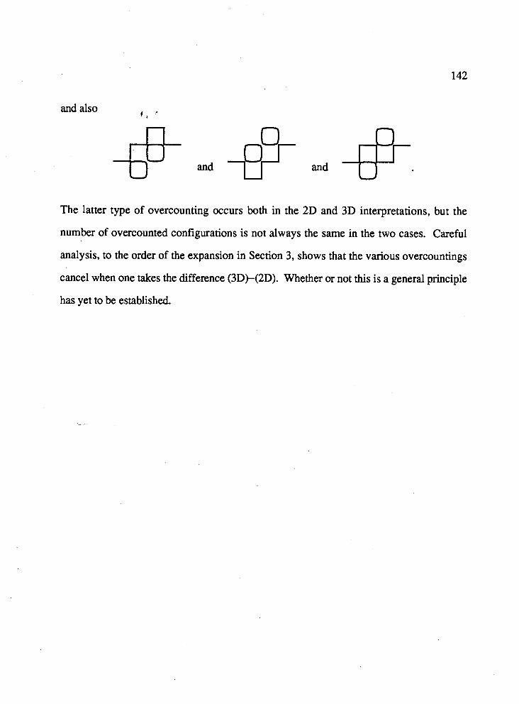
and also C ' '

The latter type of overcounting occurs both in the 2D and 3D interpretations, but the

number of overcounted configurations is not always the same in the two cases. Careful

analysis, to the order of the expansion in Section 3, shows that the various overcountings

cancel when one takes the difference (3D)-(2D). Whether or not this is a general principle

has yet to be established.

References Z , '

Abraham, D. B. (1986). In "Phase Transitions and Critical Phenomena", Vol. 10 (C. Domb and J. L. Lebowitz, eds.), pp. 2-69. Academic, New York.

Adler, J. (1987). Phys. Rev. B 36, 2473.

Akutsu, N. and Akutsu, Y. (1987a). J. Phys. Soc. Jpn. 56, 1443.

Akutsu, N. and Akutsu, Y. (1987b). J. Phys. Soc. Jpn. 56,2248.

Andreev, A. F. (1981). Zh. Eksp. Teor. Fiz. 80,2042 [Sov. Phys. JETP 53, 1063 (1982)l.

Avron, J. E. and Zia, R. K. P. (1988). Phys. Rev. B 37, 661 1.

Avron, J. E., Taylor, J. E. and Zia, R. K. P. (1983). J. Stat, Phys. 33, 493.

Avron, J. E.,van Beijeren, H., Schulman, L. S. and Zia, R. K. P. (1982). J. Phys. A 15, L81.

Balibar, S., and Castaing, J. (1980). Phys. kzt, 41, L329.

Burgoyne, P. N. (1963). J. Math. Phys. 4, 1320.

Burton, W. K., Cabrera, N. and Frank, F. C. (1951). Bhilos. Trans. Roy. Soc. London, Ser. A243, 299.

Cabrera, N. (1964). Sur$ Sci, 2, 320. L--..

Caginalp, G. and Fisher, M. E. (1979). Commun. Math. Phys. 65,247.

Calheiros, F., Johannesen, S. and Merlini, D. (1987). J. Phys. A 20,5991. . .

Callen, H. B. (1960). "Thermodynamics". John Wiley & Sons, New York.

Cheng H. and Wu, T. T. (1967). Phys. Rev. 164,719.

Chui, S. T. and Weeks, J. D. (1976). Phys. Rev. B 14, 4978.

Curie, P. (1885). Bull. Soc. Mineralog. de France 8, 145.

Dinghas, A. (1944). Zeits, f. Kristallog. 105,304

Dobrushin, R ~ . , .~o teck ; , R. and Shlosman, S. B. (1989). In "Stochastic Methods in Mathematics and Physics: Proceedings of the Twenty-Fourth Karpacz Winter School, Karpacz, Poland, Jan. 13-27, 1988", (R. Gielerak and W. Karwowski, eds.), pp 221-229. World Scientific, Singapore.

Fan, C. and Wu, F. Y. (1969). Phys. Rev, 179, 560.

Fan, C. and Wu, F. Y. (1970). Phys. Rev. B 2, 723.

Federer, H. (1967). "Geometric Measure Theory". Springer Verlag, New York. 8

Feller, W. (1957). "An Introduction to Probability Theory and Its Applications", Vol. 1. John Wiley, New York.

Feynman, R. P. (1972). "Statistical Mechanics", pp 136-150. Benjamin/Cumrnings, Reading, Mass.

Fisher, D. S. and Weeks, J. D. (1983). Phys. Rev. Lett. 50, 1077.

Fisher, M. E. (1969). J. Phys. Soc. Japan (Suppl.) 26, 87.

Fisher, M. E. and Caginalp, G. (1977). Commun. Math. Phys. 56, 11.

Fisher, M. E. and Ferdinand, A. E. (1967). Phys. Rev. Lett. 19, 169.

Fradkin, E. (1983). Phys. Rev. B 28, 5338.

Fradkin, E., Huberman, B. A. and Shenker, S. H. (1978). Phys. Rev. B 18, 4789.

Gallet, F., NoziiYes, P., Balibar, S. and Rolley, E. (1986). Europhys. Lett. 2, 70 1.

Gaunt, D. S. and Guttrnann, A. J. (1974). In "Phase Transitions and Critical Phenomena", Vol. 3 (C. Domb and M. S. Green, eds.), pp. 181-243. Academic, New York.

Griffiths, R. B. (1980). In "Phase Transitions in Surface Films", (J. G. Dash and J. Ruvalds, eds.), pp. 1-27. Plenum, New York.

Herring, C. (1951). Phys. Rev. 82, 87.

Hemng, C. (1953). In "Structure and Properties of Solid Surfaces", (R. Gomer and G. Smith, eds.), pp 5-81. Chicago Univ. Press, Chicago.

Heyraud, J. C. and Mbtois, J. J. (1983). Surf. Sci. 128, 334.

Hilton, H. (1903). "Mathematical Crystallography". Oxford.

Holzer, M. (1990a). Phys. Rev. Lett. 64, 653.

Holzer, M. (1990b). "Exact Equilibrium Crystal Shapes in Two Dimensions for Free- Fermion Models", Simon Fraser University preprint.

Holzer, M. and Wortis, M. (1989). Phys. Rev. B 40, 1 1044.

Hurst, C. A. (1966). J. Math. Phys. 7 , 305.

Hurst, C. A. and Green, H. S. (1960). J. Chem. Phys. 33, 1059.

Huse, D. A., van Saarloos, W. and Weeks, J. D. (1985). Phys. Rev. B 32, 233.

Jayaprakash, C. and Saam, W. F. (1984a). Phys. Rev. B 30, 3916.

Jayaprakash, C., Rottman, C. and Saam, W. F. (1984b). Phys. Rev. B 30,6549. 4 , *

Jayaprakash, C., Saam, W. F. and Teitel, S. (1983). Phys. Rev. Lett. 50, 2017.

Kac, M. and Ward, J. C. (1952). Phys Rev. 88, 1332.

Kano, K. and Naya, S. (1953). Prog. Theor. Phys. 10, 158.

Kasteleyn, P. W. (1961). Physica 27,1209.

Kasteleyn, P. W. (1963). J. Math. Phys. 4 , 287.

Keshishev, K.O., Parshin, A. Ya., and Babkin, A.V. (1981). Sov. Phys. JETP 53,362.

Kosterlitz, J. M. and Thouless. D. J. (1973). J. Phys. C 6, 1 181.

Kotecki, R. (1988). In "Proceedings of the Ninth International congress of mathematical physics", (B. Simon, I.M. Davies, and A. Truman, eds.). Hilger, Bristol, England.

Kramers, H. A. and Wannier, G. K. (1941). Phys. Rev. 60, 252.

Landau, J, Lipson, S.G., Maattanen, L.M., Balfour, L.S., and Edwards, D.O. (1980). Phys Rev. Lett. 45, 31.

Landau, L. D. and Lifshitz, E. M. (1968). "Statistical Physics", 2nd edn., pp 447-454. Pergamon, Oxford.

Leamy, H. J., Gilmer, G. H. and Jackson, K. A. (1975). In "Surface Physics of Crystalline Materials", p. 169. Academic, New York.

Lieb, E. H. (1967). Phys. Rev. Lett. 19, 108.

Lieb, E. H. and Wu, F.Y. (1972). In "Phase Transitions and Critical Phenomena", Vol. 1. (C. Domb and M. S. Green, eds.). Academic, New York.

Liebmann, H. (19 14). Zeits. f. Kristallog. 53, 17 1.

McCoy, B. and Wu, T. T. (1973). "The Two Dimensional Ising Model", pp. 299-305. Harvard, Cambridge, Mass.

Minkowski, H (1903). Math. Ann. 57, 447.

Minkowski, H (191 1). "Gesammelte Abhandlungen". B.G. Teubner, Leipzig und Berlin.

Mon, K. K., Wansleben, S., Landau, D. P. and Binder, K. (1988). Phys. Rev. Lett. 60, 708.

Mon, K. K., Wansleben, S., Landau, D. P. and Binder, K. (1989). Phys. Rev. B 39, 7089.

Morita, T. (1986). J. Phys. A 19, 1197 (1986).

Onsager, L. (1944). Phys. Rev. 65, 117.

Pawley, G. S., Syesdsen, R. H. D., Wallace, J. and Wilson, K. G. (1984). P h p . Rev. B 29, 4030."

Pokrovsky, V. L. and Talapov, A.L. (1979). Phys. Rev. Lett. 42,65.

Rottman, C. and Wortis, M. (1981). Phys. Rev. B 24, 6274.

Rottman, C. and Wortis, M. (1984a). Phys. Rep. 103,59.

Rottman, C. and Wortis, M. (1984b). Phys. Rev. B 29, 328.

Ryazanov, G. V. (1970). Zh. Eksp. Teor. Fiz. 59, 1000 [Sov. Phys. JETP 32, 544 (197 I)].

Shaw, L. J. and Fisher, M. E. (1989). Phys. Rev. A 39, 2189.

Sherman, S. (1960). J. Math. Phys. 1, 202.

Sherman, S. (1963). J. Math. Phys. 4, 1213.

Shi, A.-C. and Wortis, M. (1988). Phys. Rev. B 37, 7793.

Slater, J. (1941). Chem Phys. 9, 16.

Sutherland, B. (1967). Phys. Rev. Lett. 19, 103.

Sutherland, B. (1970). J. Math. Phys. 11, 3183.

Swendsen, R. H. (1978). Phys. Rev. B17, 3710 . Syozi, I. (1972). In "Phase Transitions and Critical Phenomena", Vol. 1 (C. Domb and

M. S. Green, eds.), pp. 269-329. Academic, New York.

Taylor, J. E. (1974). Symposia Mathematics 14,499.

Taylor, J. E. (1978). Bull. Amer. Math. Soc. 84, 568.

Temperley, H. N. V. and Fisher, M. E. (1961). Phil. Mag. 6, 1061.

Vaidya, H. G. (1976). Phys. Lett. 57A, 1.

Vaks, V. G., Larkin, A. L. and Ovchinnikov, Yu N. (1965). Zh. eksp. theo. Fiz. 49, 1180 (Soviet Phys. JETP 22, 820 (1966)).

van Beijeren, H. (1977). Phys. Rev. Lett. 38, 993.

van Beijeren, H. and Nolden, I. (1987). In "Topics in Current Physics", Vol. 43 (W. Schommers and P. von Blanckenhagen, eds.), pp. 259-300. Springer Verlag, Berlin.

van der Eerden, J. P. and Knops, H. J. F. (1978). Phys. Lett. 66A, 334.

Vdovichenko, N. V. (1964). Zh. Eksp. Teor. Fiz. 47,715 [Sov. p h p . JETP 20, 477 (l965)I.

von Laue, M. (1243). Zeits. f. Kristallog. 105, 124. I

Watson, P. G. (1968). J. Phys. C 1, 575.

Weeks, J. D. (1980). In "Ordering in Strongly Fluctuating Condensed Matter Systems", (T. Riste, ed.). Plenum, New York.

Weeks, J. D., Gilmer, G. H. and Leamy, H. J. (1973). Phys. Rev. Lett. 31, 549.

Whitney, H. (1937). Composito Mathematica 4,276.

Widom, B. (1965). J. Chem. Phys. 43, 3892.

Wolf, P.E., Balibar, S. and Gallet, F. (1983). Phys. Rev. Lett. 51, 1366.

Wortis, M. (1988). In "Chemistry and Physics of Solid Surfaces", Vol. VII (R. Vanselow, ed.), pp. 367-405. Springer Verlag, Berlin.

Wu, F. Y. (1967). Phys. Rev. Lett. 18, 605.

Wu, F. Y. (1968). Phys. Rev. 168, 539.

Wulff, G. (1901). Zeits. f. Kristallog. 34, 449.

Zia, R. K. P. (1978). Phys. Lett. 64A, 345.

Zia, R. K. P. (1984). In "Proceedings of the Twenty-Sixth Scottish Universities Summer School in Physics on Statistical and Particle Physics: Common Problems and Techniques, Edinburgh, 1983", (K. C. Bowler and A. J. McKane, eds.), pp. 247- 301. Scottish Universities Summer School in Physics, Edinburgh.

Zia, R. K. P. (1986). J. Stat. Phys. 45, 801.

Zia, R. K. P. (1988). In "Proceedings of the 1988 Workshop on Statistical Mechanics, Academia Sinica, Taiwan", (C. K. Hu, ed.). World Scientific, Singapore.

Zia, R. K. P. and Avron, J. E. (1982). Phys. Rev. B 25, 2042.

Zia, R. K. P. and Gittis, A. (1987). Phys. Rev. B 35, 5907.