Embed Size (px)
Citation preview

Exact Simulation Techniques in Applied Probabilityand Stochastic Optimization
Yanan Pei
Submitted in partial fulfillment of the
requirements for the degree
of Doctor of Philosophy
in the Graduate School of Arts and Sciences
COLUMBIA UNIVERSITY
2018

c©2018
Yanan Pei
All Rights Reserved

ABSTRACT
Exact Simulation Techniques in Applied Probabilityand Stochastic Optimization
Yanan Pei
This dissertation contains two parts. The first part introduces the first class of perfect sampling
algorithms for the steady-state distribution of multi-server queues in which the arrival process is a
general renewal process and the service times are independent and identically distributed (iid); the
first-in-first-out FIFO GI/GI/c queue with 2 ≤ c <∞. Two main simulation algorithms are given
in this context, where both of them are built on the classical dominated coupling from the past
(DCFTP) protocol. In particular, the first algorithm uses a coupled multi-server vacation system
as the upper bound process and it manages to simulate the vacation system backward in time from
stationarity at time zero. The second algorithm utilizes the DCFTP protocol as well as the Random
Assignment (RA) service discipline. Both algorithms have finite expected termination time with
mild moment assumptions on the interarrival time and service time distributions. Our methods
are also extended to produce exact simulation algorithms for Fork-Join queues and infinite server
systems.
The second part presents general principles for the design and analysis of unbiased Monte Carlo
estimators in a wide range of settings. The estimators possess finite work-normalized variance
under mild regularity conditions. We apply the estimators to various applications including un-
biased steady-state simulation of regenerative processes, unbiased optimization in Sample Average
Approximations and distribution quantile estimation.

Table of Contents
List of Figures v
List of Tables vi
Acknowledgements vii
1 Introduction 1
I Exact Simulation of Multi-Dimensional Queueing Models with Renewal
Input 3
2 Introduction to Part I 4
3 Exact Simulation with Vacation Systems 8
3.1 Simulation strategy and main result . . . . . . . . . . . . . . . . . . . . . . . . . . . 8
3.1.1 Elements of the simulation strategy: upper bound and coupling . . . . . . . . 9
3.1.2 Monotonicity properties and the stationary GI/GI/c queue . . . . . . . . . . 13
3.1.3 Description of simulation strategy and main result . . . . . . . . . . . . . . . 17
3.2 Coalescence detection in finite time . . . . . . . . . . . . . . . . . . . . . . . . . . . . 18
3.3 Simulation procedure . . . . . . . . . . . . . . . . . . . . . . . . . . . . . . . . . . . . 23
3.3.1 Simulate a random walk with negative drift jointly with “milestone” events . 28
3.3.2 Simulate the vacation system between inspection times . . . . . . . . . . . . . 30
3.3.3 Overall exact simulation procedure . . . . . . . . . . . . . . . . . . . . . . . . 31
3.4 Numerical experiments . . . . . . . . . . . . . . . . . . . . . . . . . . . . . . . . . . . 32
i

4 Exact Simulation with Random Assignment 37
4.1 The FIFO and RA GI/GI/c model . . . . . . . . . . . . . . . . . . . . . . . . . . . . 37
4.1.1 The FIFO GI/GI/c model . . . . . . . . . . . . . . . . . . . . . . . . . . . . 37
4.1.2 The RA GI/GI/c model . . . . . . . . . . . . . . . . . . . . . . . . . . . . . . 38
4.2 Simulating exactly from the stationary distribution of the RA GI/GI/c model . . . 41
4.2.1 Algorithm for simulating exactly from π for the FIFO GI/GI/c queue: The
case P (A > V ) > 0 . . . . . . . . . . . . . . . . . . . . . . . . . . . . . . . . . 45
4.2.2 Why we can assume that interarrival times are bounded . . . . . . . . . . . . 46
4.2.3 A more efficient algorithm: sandwiching . . . . . . . . . . . . . . . . . . . . . 48
4.2.4 Continuous-time stationary constructions . . . . . . . . . . . . . . . . . . . . 51
4.3 Numerical experiments . . . . . . . . . . . . . . . . . . . . . . . . . . . . . . . . . . . 53
4.4 Infinite server systems and other service disciplines . . . . . . . . . . . . . . . . . . . 57
4.5 Fork-Join models . . . . . . . . . . . . . . . . . . . . . . . . . . . . . . . . . . . . . . 59
4.6 The case when P (A > V ) = 0: Harris recurrent regeneration . . . . . . . . . . . . . 60
II Unbiased Monte Carlo Computations and Applications 62
5 Introduction to Part II 63
5.1 The general principles . . . . . . . . . . . . . . . . . . . . . . . . . . . . . . . . . . . 65
6 Unbiased Multi-level Monte Carlo 70
6.1 Non-linear functions of expectations and applications . . . . . . . . . . . . . . . . . . 71
6.1.1 Application to steady-state regenerative simulation . . . . . . . . . . . . . . . 75
6.1.2 Additional applications . . . . . . . . . . . . . . . . . . . . . . . . . . . . . . 76
6.2 Stochastic convex optimization . . . . . . . . . . . . . . . . . . . . . . . . . . . . . . 77
6.2.1 Unbiased estimator of optimal solution . . . . . . . . . . . . . . . . . . . . . . 80
6.2.2 Unbiased estimator of optimal value . . . . . . . . . . . . . . . . . . . . . . . 84
6.2.3 Applications and numerical examples . . . . . . . . . . . . . . . . . . . . . . . 86
6.3 Quantile estimation . . . . . . . . . . . . . . . . . . . . . . . . . . . . . . . . . . . . 89
ii

III Bibliography 92
Bibliography 93
IV Appendices 98
A Appendix to Chapter 3 99
A.1 The iid property of the coupled service times and independence of the arrival process 99
A.2 Proof of technical lemmas of monotonicity . . . . . . . . . . . . . . . . . . . . . . . . 102
B Appendix to Chapter 4 104
B.1 Detailed algorithm steps in Section 4.2.1 . . . . . . . . . . . . . . . . . . . . . . . . . 104
B.1.1 Simulation algorithm for the process Y−n : n ≥ 0 . . . . . . . . . . . . . . . 105
B.1.2 Simulation algorithm for the process X−n : n ≥ 0 . . . . . . . . . . . . . . . 111
B.1.3 Simulation algorithm for S(r)n : n ≥ 0 and coalescence detection . . . . . . . 115
B.2 Proof of propositions . . . . . . . . . . . . . . . . . . . . . . . . . . . . . . . . . . . . 116
iii

List of Figures
3.1 Renewal processes . . . . . . . . . . . . . . . . . . . . . . . . . . . . . . . . . . . . . 11
3.2 The relationship between the renewal processes and the random walks (a) N0(t)−atand S
(0)n (b) (a/c)t−N i(t) and S
(i)n . . . . . . . . . . . . . . . . . . . . . . . . . . . 25
3.3 This figure plots a realization of the sample path S(0)n : 0 ≤ n ≤ 11. Here we set
m = 1 and L = 3. Then, Φ01 = 3, Υ0
1 = 4, Φ02 = 7. If Υ0
2 = ∞, then for n ≥ 7,
S(0)n will stay below the level S
(0)7 + m, which is demonstrated by the bold dashed
line. Thus, M(0)2 = maxn≥2S(0)
n = S(0)2 by only comparing the random walk values
between step 2 and step 7. . . . . . . . . . . . . . . . . . . . . . . . . . . . . . . . . . 27
3.4 Number of customers for an M/M/c queue in stationarity when λ = 3, µ = 2 and
c = 2. . . . . . . . . . . . . . . . . . . . . . . . . . . . . . . . . . . . . . . . . . . . . 33
3.5 Number of customers for an M/M/c queue in stationarity when λ = 10, µ = 2 and
c = 10. . . . . . . . . . . . . . . . . . . . . . . . . . . . . . . . . . . . . . . . . . . . . 34
3.6 Number of customers for an Erlang(k1, λ)/Erlang(k2, µ)/c queue in stationarity when
k1 = 3, λ = 4.5, k2 = 2, µ = 2/3, c = 5 and ρ = 0.9. . . . . . . . . . . . . . . . . . . . 34
4.1 Number of customers for an M/M/c queue in stationarity when λ = 3, µ = 2, c = 2. 54
4.2 Number of customers for an M/M/c queue in stationarity when λ = 10, µ = 2, c = 10. 54
4.3 Number of customers for an Erlang(k1, λ)/Erlang(k2, µ)/c queue in stationarity
when k1 = 2, λ = 9, k2 = 2, µ = 5, c = 2 and ρ = 0.9. . . . . . . . . . . . . . . . . . 55
4.4 Distributions of time taken to detect coalescence under two algorithms for an M/M/c
queue . . . . . . . . . . . . . . . . . . . . . . . . . . . . . . . . . . . . . . . . . . . . 56
6.1 Linear regression test on Beijing’s PM2.5 data . . . . . . . . . . . . . . . . . . . . . 87
iv

6.2 Logistic regression test on AOL’s campaign data . . . . . . . . . . . . . . . . . . . . 88
A.1 Matching procedure of service times to arrival process . . . . . . . . . . . . . . . . . 100
v

List of Tables
3.1 Simulation estimates for the mean coalescence time of M/M/c queue (QD) . . . . . 35
3.2 Simulation estimates for the mean coalescence time of M/M/c queue (QED) . . . . 35
3.3 Simulation result for computational complexities with varying traffic intensities . . . 36
4.1 Simulation result for computational complexities with varying traffic intensities . . . 57
vi

Acknowledgments
First and foremost, I would like to express my gratitude to my advisor Professor Jose Blanchet
for his enthusiastic inspiration, patient guidance and continuous support through the five years of
studies and research. Jose is a talented researcher, an insightful mentor and a caring friend. It has
been an honor and a privilege working with Jose closely over my entire PhD years, and I enjoy
every discussion with him as he always impress me with his ample knowledge, keen intuition and
deep passion for research. The strong example he has set will continue to inspire me to stay curious,
be passionate and strive towards excellence in my future work and life.
I am grateful to Professor Karl Sigman, Professor Ton Dieker, Professor Jing Dong and Professor
Henry Lam for generously offering their time serving on my dissertation committee and providing
invaluable advice. Special thanks go to Professor Jing Dong and Professor Karl Sigman, whom
I collaborated along with Jose in the work of Chapter 3 and 4. I also want to thank Professor
Xinyun Chen, with whom I worked on another research project about applying stochastic analysis
techniques to uncover the structure of limit order books in financial markets. Although I finally
decided not to include that work in the thesis because of the topic difference, I do appreciate this
research experience, as it enlightened me on huge possibilities of connecting theories from academia
to various practices in industry.
I would like to extend my sincere thanks to all the amazing professors who have taught me at
Columbia University for sharing their knowledge without reservation, and all the members of staff
at the department of IEOR for creating such a friendly and supportive environment.
Thanks to all my friends at Columbia, this journey has been colorful and enjoyable with your
company. I will always cherish the memories of us attending the same courses, preparing qualifi-
cation exams, discussing research ideas, exploring the great New York City, and sharing tears and
joy together. My PhD life would be dull without you and I sincerely hope our friendship will last
lifelong.
vii

Lastly and most importantly, I owe my deepest gratitude towards my parents and grandmother,
for their unconditional love and endless support throughout my life. They are my constant source
of inspiration and strength. Special thanks to my husband for always believing in me and cheering
me up. I would like to dedicate this work to them.
viii

To Xiaoqin Liu, Yongqiang Pei, Luming Wang
ix

CHAPTER 1. INTRODUCTION 1
Chapter 1
Introduction
This dissertation studies various bias-removal simulation techniques in applied probability and
stochastic optimization problems. These techniques are developed based on a wide range of clas-
sic tools including queueing theory, steady-state analysis, perfect sampling, large deviation theory,
multi-level Monte Carlo and sample average approximations. By different natures of such tech-
niques, we divide the dissertation into two main parts.
Part I presents two sets of algorithms for simulating exactly from the stationary distribution of
multi-server queues with general interarrival time and service time distributions in finite expected
run time, and our work closes a gap in the perfect sampling literature. Perfect sampling aims to
sample without any bias from the steady-state distribution of a given ergodic process, and it has
evolved as a powerful way of sampling from stationary distributions of queueing models for which
such distributions can not be derived explicitly. Both of the algorithms are developed by utilizing
a perfect sampling protocol named Dominated Coupling From The Past (DCFTP), yet they are
significantly different by design; one solves the problem by using a coupled multi-server vacation
system as the upper bound process while the other directly simulates the Random Assignment
(RA) model backward in time. We will have a thorough discussion about the background and
relevant literatures of perfect sampling in Chapter 2, then we describe the two sets of algorithms
respectively in Chapter 3 and Chapter 4.
Part II presents general de-biasing principles for Monte Carlo computations based on the multi-
level Monte Carlo method and the bias removal ideas studied in the literature. Within the general
framework, we propose unbiased estimators to various applied probability and operations research

CHAPTER 1. INTRODUCTION 2
settings such as steady-state simulation of regenerative processes, stochastic convex optimization,
and distribution quantiles estimation. A key contribution of the development of such unbiased
estimators is that it enables the use of parallel computing to improve the estimation accuracy and
computation efficiency. In Chapter 5, we review the literatures and give the general principles to
provide the high-level intuition. In Chapter 6, we discuss the construction of unbiased estimators
for different settings of interest.

3
Part I
Exact Simulation of
Multi-Dimensional Queueing Models
with Renewal Input

CHAPTER 2. INTRODUCTION TO PART I 4
Chapter 2
Introduction to Part I
In this part, we present two exact simulation algorithms for the steady-state distribution of multi-
server queues with general interarrival time and service time distributions. Both of our algorithms
have finite expected termination time under the assumption that the interarrival times and service
times have finite 2 + ε moments for some ε > 0.
In recent years, the method of exact simulation has evolved as a powerful way of sampling from
stationary distribution of a given ergodic process for which such distributions cannot be derived
explicitly. The most popular perfect sampling protocol, known as Coupling From The Past (CFTP),
was introduced in the seminal paper [Propp and Wilson, 1996]; see also [Asmussen et al., 1992]
for another important early reference on perfect simulation. Foss and Tweedie [Foss and Tweedie,
1998] proved that CFTP can be applied if and only if the underlying process is uniformly ergodic,
which is not a property applicable to multi-server queues. So, we use a variation of the CFTP
protocol called Dominated CFTP (DCFTP) introduced by Kendall in [Kendall, 1998] and later
extended in [Kendall and Møller, 2000; Kendall, 2004].
A typical implementation of DCFTP requires at least four ingredients:
(a) a stationary upper bound process for the target process,
(b) a stationary lower bound process for the target process,
(c) the ability to simulate (a) and (b) backward in time (i.e., from time 0 to −t, for any t > 0),
(d) a finite time −T < 0 at which the state of the target process is determined (typically by

CHAPTER 2. INTRODUCTION TO PART I 5
having the upper and lower bound processes coalesce), and the ability to reconstruct the
target process from −T up to time 0 coupled with the two bounding processes.
The time −T is called the coalescence time, and it is desirable to have E [T ] <∞. The ingredients
are typically combined as follows. One simulates (a) and (b) backward in time (by applying (c))
until the processes meet. The target process is sandwiched between (a) and (b). Therefore, if we
can find a time −T < 0 when processes (a) and (b) coincide, the state of the target process is
known at −T as well. Then, applying (d), we reconstruct the target process from −T up to time
0. The algorithm outputs the state of the target process at time 0.
It is quite intuitive that the output of the above construction is stationary. Specifically, assume
that the sample path of the target process coupled with (a) and (b) is given from (−∞, 0]. Then,
we can think of the simulation procedure in (c) as simply observing or unveiling the paths of (a)
and (b) during [−t, 0]. When we find a time −T < 0 at which the paths of (a) and (b) take the
same value, because of the sandwiching property, the target process must share this common value
at −T . Starting from that point, property (d) simply unveils the path of the target process. Since
this path has been coming from the infinite distant past (we simply observed it from time −T ), the
output is stationary at time 0. Notice that while −T is a random time, the output is the state of
the target process at the fixed time 0.
One can often improve the performance of a DCFTP protocol if the underlying target process
is monotone [Kendall, 2004], as in the multi-server queue setting. A process is monotone if there
exists a certain partial order, , such that if w and w′ are initial states where w w′, and one uses
common random numbers to simulate two paths, one starting from w and the other from w′, then
the order is preserved when comparing the states of these two paths at any point in time. Thus,
instead of using the bounds (a) and (b) directly to detect coalescence, one could apply monotonicity
to detect coalescence as follows: At any time −t < 0, one can start two paths of the target process,
one from the state w′ obtained from the upper bound (a) observed at time −t, and the other from
the state w w′ obtained from the lower bound (b) observed at time −t. Then, we run these two
paths using common random numbers, which are consistent with the backward simulation of (a)
and (b), in reverse order according to the dynamics of the target process, and check whether these
two paths meet before time zero. If they do, the coalescence occurs at such a meeting time. We
also notice that because we are using common random numbers and system dynamics, these two

CHAPTER 2. INTRODUCTION TO PART I 6
paths will merge into a single path from the coalescence time forward, and the state at time zero
will be the desired stationary draw. If coalescence does not occur, then one can simply let t← 2t,
and repeat the above procedure. For this iterative search procedure, we must show that the search
terminates in finite time.
While the DCFTP protocol is relatively easy to understand, its application is not straightfor-
ward. In most applications, the most difficult part has to do with element (c). Then, there is an
issue of finding good bounding processes (elements (a) and (b)), in the sense of having short coa-
lescence times – which we interpret as making sure that E [T ] <∞. There has been a substantial
amount of research that develops generic algorithms for Markov chains (see, for example, [Corcoran
and Tweedie, 2001] and [Connor and Kendall, 2007]). These methods rely on having access to the
transition kernels, which are difficult to obtain in our case. Perfect simulation for queueing systems
has also received a significant amount of attention in recent years, though most perfect simulation
algorithms for queues impose Poisson assumptions on the arrival process. Sigman [Sigman, 2011;
Sigman, 2012] applied the DCFTP and regenerative idea to develop perfect sampling algorithms for
stable M/G/c queues. The algorithm in [Sigman, 2011] requires the system to be super-stable (i.e.,
the system can be dominated by a stable M/G/1 queue). The algorithm in [Sigman, 2012] works
under natural stability conditions by using a forward time regenerative method (a general method
developed in [Asmussen et al., 1992]) and using the M/G/c model under a random assignment
(RA) discipline as an upper bound, but it has infinite expected termination time. A recent work
by Connor and Kendall [Connor and Kendall, 2015] extends Sigman’s algorithm [Sigman, 2012] by
using the RA model. They accomplish this by first exactly simulating the RA model in stationary
backward in time under process sharing (PS) at each node, then reconstructing it to obtain the
RA model with FIFO at each node and doing so in such a way that a sample-path upper bound of
the FIFO M/G/c queue is achieved. Their algorithm has finite expected termination time, but it
still requires the arrivals to be Poisson. The main reason for the Poisson arrival assumption is that
under this assumption, one can find dominating processes which are quasi-reversible (see Chapter
3 of [Kelly, 1979]) and therefore can be simulated backward in time using standard Markov chain
constructions (element (c)).
In general, constructing elements (a) and (b), (a) in particular, as (b) can often be taken as
the trivial lower bound, 0, in the multi-server queue setting requires proving sample path (almost

CHAPTER 2. INTRODUCTION TO PART I 7
sure) dominance under different service/routing disciplines. The sample path method has been
widely used in the control of queues [Liu et al., 1995]. Comparison of multi-server queues, under
the almost sure dominance or the stochastic dominance, has been studied in the literature (see, for
example, [Wolff, 1977; Foss, 1980; Foss and Chernova, 2001] and references therein).
For general renewal arrival process, our work is close in the spirit to [Ensor and Glynn, 2000],
[Blanchet and Dong, 2013] and [Blanchet and Wallwater, 2015], but the models treated are funda-
mentally different. Thus, it requires some new developments.
For the first algorithm, we use a different coupling construction than that introduced in [Sigman,
2012] and refined in [Connor and Kendall, 2015]. In particular, we take advantage of a vacation
system which allows us to transform the problem into simulating the running infinite horizon
maximums (from time t to infinity) of renewal processes, compensated with negative drifts so that
the infinite horizon maximums are well defined. Finally, we note that a significant advantage of our
method, in contrast to [Sigman, 2012], is that we do not need to wait until the upper bound system
empties to achieve coalescence. Due to the monotonicity of our process, we can apply the iterative
method introduced above. This is important in many-server queues in heavy traffic for which it
would take an exponential amount of time (in the arrival rate), or sometimes be impossible, to
observe an empty system.
For the second set of algorithms, we utilize DCFTP by directly simulating the RA model in
reverse-time (under FIFO at each node). The method involves extending, to a multi-dimensional
setting, a recent result of [Blanchet and Wallwater, 2015] for exactly simulating the maximum of
a negative drift random walk endowed with iid increments. An initial version of the algorithm is
to simulate the upper bound process backward in time until an empty system is detected; then a
more efficient “sandwiching” algorithm is given to deal with the cases where the empty status is
difficult or impossible to observe. We also remark on how our approach can lead to new results
for other models too, such as infinite server queues, multi-server queues under the last-in-first-out
(LIFO) discipline, or the randomly choose next discipline, and even Fork-Join models (also called
split and match models).
CHAPTER 3. EXACT SIMULATION WITH VACATION SYSTEMS 8
Chapter 3
Exact Simulation with Vacation
Systems
We give our first exact simulation algorithm, which utilizes a so-called “vacation system” as an
upper bound, in this chapter. In Section 3.1 we describe our simulation strategy, involving elements
(a) – (d), and we conclude the section with the statement of a result which summarizes our main
contribution (Theorem 1). Subsequent sections (Sections 3.2 and 3.3) provide more details of our
simulation strategy. In Section 3.4, we conduct some numerical experiments. Appendix A contains
the proofs of some technical results.
3.1 Simulation strategy and main result
Our target process is the stationary process generated by a multi-server queue with iid interarrival
times and iid service times which are independent of the arrivals. There are c ≥ 1 identical servers,
each can serve at most one customer at a time. Customers are served on a first-in-first-out (FIFO)
basis. Let G(·) and G(·) = 1 − G(·) (resp. F (·) and F (·) = 1 − F (·)) denote the cumulative
distribution function, CDF, and the tail CDF of the interarrival times (resp. service times). We
shall use A to denote a random variable with CDF G, and V to denote a random variable with
CDF F .
Assumption 1. Both A and V are strictly positive with probability one, and there exists ε > 0

CHAPTER 3. EXACT SIMULATION WITH VACATION SYSTEMS 9
such that
E[A2+ε] <∞, E[V 2+ε] <∞.
The previous assumption will allow us to conclude that the coalescence time of our algorithm
has finite expectation. The algorithm will terminate with probability one if E[A1+ε]+E[V 1+ε] <∞.
We assume that G (·) and F (·) are known so that the required parameters in our algorithmic
development can be obtained. We write λ = (∫∞
0 G(t)dt)−1 = 1/E [A] as the arrival rate, and
µ = (∫∞
0 F (t)dt)−1 = 1/E[V ] as the service rate. In order to ensure the existence of the stationary
distribution of the system, we require the following stability condition: λ/(cµ) < 1.
3.1.1 Elements of the simulation strategy: upper bound and coupling
We refer to the upper bound process as the vacation system, the construction that we use is based
on that given in [Garmarnik and Goldberg, 2013]. Let us first explain in words how the vacation
system operates. Customers arrive at the vacation system according to the renewal arrival process,
and the system operates similarly to a GI/GI/c queue, except that every time a server (say server
i∗) finishes an activity (i.e., a service or a vacation), if there is no customer waiting to be served
in the queue, server i∗ takes a vacation which has the same distribution as the service times. If
there is at least one customer waiting, the first customer waiting in the queue starts to be served
by server i∗.
Using a suitable coupling, the work of [Garmarnik and Goldberg, 2013] shows that the total
number of jobs in the vacation system is an upper bound of the total number of jobs in the
corresponding multi-server queue. In this paper, we establish bounds for other system-related
processes, such as the Kiefer-Wolfowitz vectors, which are of independent interest.
We next provide more details about the vacation system. We introduce (c+ 1) time-stationary
renewal processes, which are used to describe the vacation system.
Let
T 0 := T 0n : n ∈ Z\0
be a time-stationary renewal point process with T 0n > 0 and T 0
−n < 0, n ≥ 1 (the T 0n are sorted in
a non-decreasing order in n). For n ≥ 1, T 0n represents the arrival time of the n-th customer into
the system after time zero, and T 0−n is the arrival time of the n-th customer, counting backward in

CHAPTER 3. EXACT SIMULATION WITH VACATION SYSTEMS 10
time, from time zero. We also define
T 0,+n := infT 0
m : T 0m > T 0
n,
that is, the arrival time of the next customer after T 0n . If n ≥ 1 or n ≤ −2, T 0,+
n = T 0n+1. However,
T 0,+−1 = T 0
1 . Similarly, we write
T 0,−n := supT 0
m : T 0m < T 0
n,
i.e., the arrival time of the previous customer before T 0n . Define An := T 0,+
n −T 0n for all n ∈ Z\0.
Note that An is the interarrival time between the customer arriving at time T 0n and the next
customer. An has CDF G (·) for n ≥ 1 and n ≤ −2, but A−1 has a different distribution due to the
inspection paradox. Figure 3.1 (a) provides a pictorial illustration of the renewal process T 0.
Similarly, for i ∈ 1, 2, ..., c, we introduce iid time-stationary renewal point processes
T i := T in : n ∈ Z\0.
As before, we have that T in > 0 and T i−n < 0 for n ≥ 1 with the T in sorted in a non-decreasing
order. We also define T i,+n := infT im : T im > T in and T i,−n := supT im : T im < T in. Then, we let
V in := T i,+n − T in. We assume that V i
n has CDF F (·) for n ≥ 1 and n ≤ −2. The V in are activities
(services and vacations), which are executed by the i-th server in the vacation system.
Next, we define, for each i ∈ 0, 1, ..., c, and any u ∈ (−∞,∞), a counting process
N iu (t) :=
∣∣[u, u+ t] ∩ T i∣∣ ,
for t ≥ 0, where | | denotes cardinality. Note that as T i−1 < 0 < T i1 by stationarity, N i0 (0) = 0.
In particular, the quantity N0u (t) is the number of customers who arrive during the time interval
[u, u + t] (see Figure 3.1 (b)). The quantity N iu (t) is the number of activities initiated by server
i during the time interval [u, u + t] when i 6= 0. For simplicity of the notation, let us write
N i (t) = N i0 (t) if t ≥ 0 and N i (t) = N i
t (−t) if t ≤ 0.
3.1.1.1 The upper bound process: vacation system
Let Qv(t) denote the number of people waiting in queue at time t in the stationary vacation system.
We write Qv(t−) := lims↑tQv (s) and dQv(t) := Qv(t) −Qv(t−). Also, for any t ≥ 0, i ∈ 0, ..., c

CHAPTER 3. EXACT SIMULATION WITH VACATION SYSTEMS 11
Figure 3.1: Renewal processes
(a) Definition of Ai’s
0T−10T−2
0T−30 T1
0 T20 T3
0
A−1A−3 A−2 A1 A2
(b) Defintion of N0u(t)
0T−10T−2
0T−30 T1
0 T20 T3
0t
Nt0 (−t) = 2
and each u ∈ (−∞,∞), define
N iu(t−) := lim
h↓0N iu−h (t) ,
and let dN iu (t) := N i
u(t) − N iu(t−) for all t ≥ 0 (note that as N i
u (0−) = 0, dN iu (0) should equal
N iu (0)). Similarly, for t ≤ 0, N i (t−) = N i
t
(|t|−).
We also introduce Xu(t) := N0u(t) −∑c
i=1Niu(t). For simplicity of the notation, we also write
X(t) = X0(t) if t ≥ 0, and X(t) = Xt(−t) if t ≤ 0. Then, the dynamics of (Qv (t) : t > 0) satisfy
dQv (t) = dX (t) + I (Qv (t−) = 0)
c∑i=1
dN i(t), (3.1)
given Qv (0). Note that here we are using the fact that arrivals do not occur at the same time as
the start of activity times; this is because the processes T i are independent time-stationary renewal
processes in continuous time so that T i−1 and T i1 have a density.
It follows from standard arguments of Skorokhod mapping [Chen and Yao, 2013] that, for t ≥ 0,
Qv(t) = Qv(0) +X(t)− inf0≤s≤t
(X(s) +Qv(0))− ,
where (X(s) +Qv(0))− = min (X (s) +Qv(0), 0). Moreover, using Loynes’ construction, we have
that, for t ≤ 0,
Qv(t) = sups≤t
X (s)−X (t) (3.2)
(see, for example, Proposition 1 of [Blanchet and Chen, 2015]). (Qv(t) : t ∈ (−∞,∞)) is a well-
defined process by virtue of the stability condition λ/(µc) < 1.
3.1.1.2 The coupling: extracting service times for each customer
The vacation system and the target process (the GI/GI/c queue) will be coupled by using the
same arrival stream of customers, T 0, and assuming that each customer brings his own service

CHAPTER 3. EXACT SIMULATION WITH VACATION SYSTEMS 12
time. In particular, the evolution of the underlying GI/GI/c queue is described using a sequence
of the form((T 0n , Vn
): n ∈ Z\0
), where Vn is the service time of the customer arriving at time
T 0n . In simulation, we start by simulating the upper bound process (vacation system). Thus, the
Vn must be extracted from the evolution of Qv (·) so that the same service times are matched to
the common arrival stream both in the vacation system and in the target process.
In order to match the service times to each of the arriving customers in the vacation system, we
define the following auxiliary processes: For every i ∈ 1, ..., c, any t > 0, and any u ∈ (−∞,∞),
let σiu (t) denote the number of service initiations by server i during the time interval [u, u + t].
Observe that
σiu (t) =
∫[u,u+t]
I (Qv (s−) > 0) dN iu (s− u) .
That is, we count activity initiations at time T ik ∈ [u, u + t] as service initiations if and only if
Qv(T ik−
)> 0. Once again, here we use the fact that arrival times and activity initiation times do
not occur simultaneously.
We now explain how to match service time for the customer arriving at T 0n , n ∈ Z\0. First,
such a customer occupies position Qv(T 0n
)≥ 1 when he enters the queue. Let D0
n be the delay (or
waiting time) inside the queue of the customer arriving at T 0n . Then we have that
D0n = inf
t ≥ 0 : Qv
(T 0n
)=
c∑i=1
σiT 0n
(t)
,
and therefore,
Vn =c∑i=1
V iN i(T 0
n+D0n) · dN i
(T 0n +D0
n
). (3.3)
Observe that the previous equation is valid, because for each n ∈ Z\0, there is a unique i (n) ∈1, ..., c for which dN i(n)
(T 0n +D0
n
)= 1 and dN j
(T 0n +D0
n
)= 0 if j 6= i (n) (ties are not possible
because of the time stationarity of the T i), so we obtain that (3.3) is equivalent to
Vn = Vi(n)
N i(n)(T 0n+D0
n).
We shall explain in Section A.1 that (Vn : n ∈ Z\0) and(T 0n : n ∈ Z\0
)are two independent
sequences and the Vn are iid copies of V , i.e., the extraction procedure here does not create any
bias.

CHAPTER 3. EXACT SIMULATION WITH VACATION SYSTEMS 13
3.1.2 Monotonicity properties and the stationary GI/GI/c queue
3.1.2.1 A family of GI/GI/c queues and the target GI/GI/c stationary system
We now describe the evolution of a family of standard GI/GI/c queues. Once we have the sequence((T 0n , Vn
): n ∈ Z\0
), we can proceed to construct a family of continuous-time Markov processes
(Zu(t; z) : t ≥ 0) for each u ∈ (−∞,∞), given the initial condition Zu (0; z) = z. We write z =
(q, r, e(u)), and set
Zu(t; z) := (Qu (t; z) , Ru (t; z) , Eu (t; z)) ,
for t ≥ 0, where Qu (t; z) is the number of people in the queue at time u+t (Qu (0; z) = q), Ru(t; z) is
the vector of ordered (ascending) remaining service times of the c servers at time u+t (Ru(0; z) = r),
and Eu(t; z) is the time elapsed since the previous arrival at time u+ t (Eu(0; z) = e(u)).
We shall always use Eu(0; z) = e(u) = u − supT 0n : T 0
n ≤ u, and we shall select q and r
appropriately based on the upper bound. The evolution of the process (Zu (s; z) : 0 < s ≤ t) is
obtained by feeding the traffic (T 0n , Vn
): u < T 0
n ≤ u + s for s ∈ (0, t] into a FIFO GI/GI/c
queue with initial conditions given by z. Constructing (Zu (s; z) : 0 < s ≤ t) using the traffic trace
(T 0n , Vn
): u < T 0
n ≤ u + s for s ∈ (0, t] is standard (see, for example, Chapter 3 of [Rubinstein
and Kroese, 2011]).
One can further describe the evolution of the underlying GI/GI/c queue at arrival epochs,
using the Kiefer-Wolfowitz vector [Asmussen, 2003]. In particular, for every non-negative vector
w ∈ Rc such that w(i) ≤ w(i+1) (where w(i) is the i-th entry of w) for 1 ≤ i ≤ c − 1, and each
k ∈ Z\0, the family of processes Wk
(T 0n ;w
): n ≥ k, n ∈ Z\0 satisfies
Wk
(T 0,+n ;w
)= S
((Wk
(T 0n ;w
)+ Vne1 −An1
)+), (3.4)
with initial condition Wk
(T 0k ;w
)= w, where e1 = (1, 0, ..., 0)T ∈ Rc, 1 = (1, ..., 1)T ∈ Rc, and S
is a sorting operator which arranges the entries in a vector in ascending order. In simple words,
Wk
(T 0n ;w
)for k ∈ Z\0 describes the Kiefer-Wolfowitz vector as observed by the customer
arriving at T 0n , assuming that customer who arrived at T 0
k , k ≤ n, experienced the Kiefer-Wolfowitz
state w.
Recall that the first entry of Wk
(T 0n ;w
), namely W
(1)k
(T 0n ;w
), is the waiting time of the cus-
tomer arriving at T 0n (given the initial condition w at T 0
k ). More generally, the i-th entry of

CHAPTER 3. EXACT SIMULATION WITH VACATION SYSTEMS 14
Wk
(T 0n ;w
), namely W
(i)k
(T 0n ;w
), is the virtual waiting time of the customer arriving at T 0
n if he
decides to enter service immediately after there are at least i servers free once he reaches the head
of the line. In other words, one can also interpret Wk
(T 0n ;w
)as the vector of remaining workloads
(sorted in ascending order) that would be processed by each of the c servers at T 0n , if there are no
more arrivals after time T 0n .
We are now ready to construct the stationary version of the GI/GI/c queue. Namely, for each
n ∈ Z\0 and every t ∈ (−∞,∞), we define W (n) and Z (t) via
W (n) := limk→−∞
Wk
(T 0n ; 0), (3.5)
Z (t) := (Q (t) , R (t) , E (t)) = limu→−∞
Zu (t− u, z−(u)) ,
where z−(u) = (0, 0, e(u)). We shall show in Proposition 1 that these limits are well defined.
3.1.2.2 The analogue of the Kiefer-Wolfowitz process for the upper bound system
In order to complete the coupling strategy, we also describe the evolution of the analog Kiefer-
Wolfowitz vector induced by the vacation system, which we denote by (Wv (n) : n ∈ Z\0), where
v stands for vacation. As with the i-th entry of the Kiefer-Wolfowitz vector of a GI/GI/c queue,
the i-th entry of Wv (n), namely W(i)v (n), is the virtual waiting time of the customer arriving at
time T 0n if he decides to enter service immediately after there are at least i servers free once he
reaches the head of the line (assuming that servers become idle once they see, after the completion
of current activity, the customer in queue waiting in the head of the line).
To describe the Kiefer-Wolfowitz vector induced by the vacation system precisely, let U i (t) be
the time until the next renewal after time t in T i, that is U i (t) = infT in : T in > t − t. So, for
example, U0(T 0n
)= An for n ∈ Z\0. Let U (t) =
(U1 (t) , ..., U c (t)
)T.
We then have that
Wv (n) = D0n1+S
(U((T 0n +D0
n
)−
)). (3.6)
In particular, note that W(1)v (n) = D0
n, i.e., the delay the customer arriving at T 0n would experience.
We next introduce a recursive way of constructing/defining the Kiefer-Wolfowitz vector induced by
the vacation system. We define
Wv (n) = Wv (n) + Vne1 −An1,
CHAPTER 3. EXACT SIMULATION WITH VACATION SYSTEMS 15
and let W(i)v (n) to be the i-th entry of Wv (n). Let Wv (n+) denote the Kiefer-Wolfowitz vector
seen by the customer arriving at T 0,+n . From the definition of Wv (n), we have
Wv (n+) = S((Wv (n)
)++ Ξn
),
where
Ξ(i)n = I(W (i)
v (n) < 0) · U ji(n)((T 0,+n
)−
)(i.e., ji (n) is the server whose remaining activity time immediately before T 0
n is the i-th smallest
in order).
So, (3.6) actually satisfies
Wv (n+) = S((Wv (n) + Vne1 −An1)+ +Ξn
), (3.7)
where Ξn =(
Ξ(1)n , ...,Ξ
(c)n
)T.
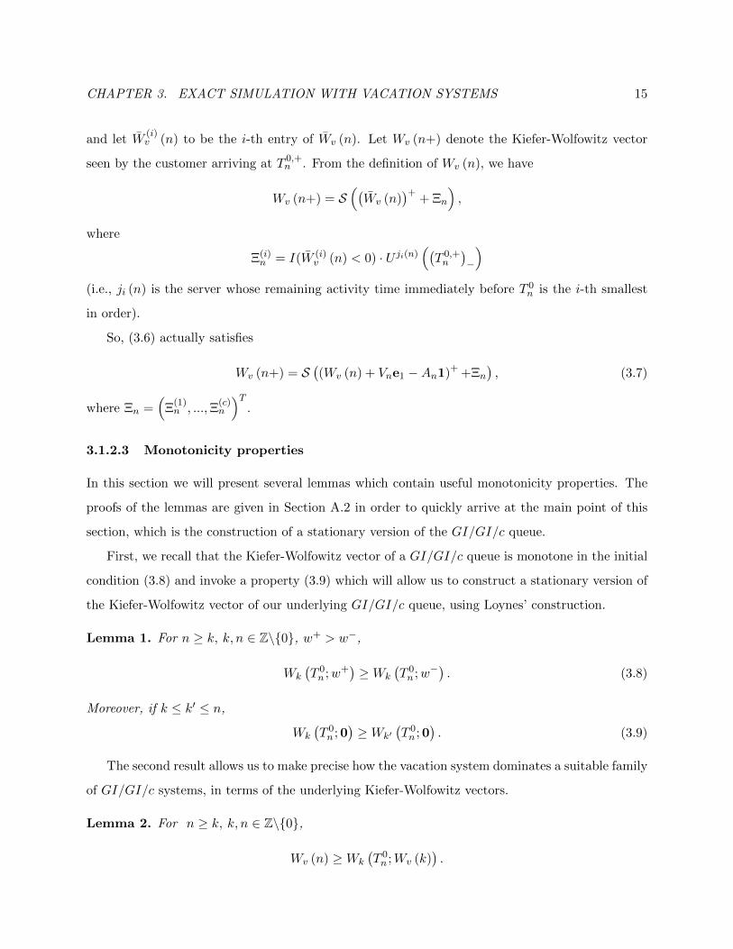
3.1.2.3 Monotonicity properties
In this section we will present several lemmas which contain useful monotonicity properties. The
proofs of the lemmas are given in Section A.2 in order to quickly arrive at the main point of this
section, which is the construction of a stationary version of the GI/GI/c queue.
First, we recall that the Kiefer-Wolfowitz vector of a GI/GI/c queue is monotone in the initial
condition (3.8) and invoke a property (3.9) which will allow us to construct a stationary version of
the Kiefer-Wolfowitz vector of our underlying GI/GI/c queue, using Loynes’ construction.
Lemma 1. For n ≥ k, k, n ∈ Z\0, w+ > w−,
Wk
(T 0n ;w+
)≥Wk
(T 0n ;w−
). (3.8)
Moreover, if k ≤ k′ ≤ n,
Wk
(T 0n ; 0
)≥Wk′
(T 0n ; 0
). (3.9)
The second result allows us to make precise how the vacation system dominates a suitable family
of GI/GI/c systems, in terms of the underlying Kiefer-Wolfowitz vectors.
Lemma 2. For n ≥ k, k, n ∈ Z\0,
Wv (n) ≥Wk
(T 0n ;Wv (k)
).

CHAPTER 3. EXACT SIMULATION WITH VACATION SYSTEMS 16
The next result shows that in terms of queue length processes, the vacation system also domi-
nates a family of GI/GI/c queues, which we shall use to construct the upper bounds.
Lemma 3. Let q = Qv(u), r = S (U (u)), and e = u− supT 0n : T 0
n ≤ u, so that z+ = (q, r, e) and
z− = (0,0, e) then for t ≥ u,
Qu(t− u; z−) ≤ Qu(t− u; z+) ≤ Qv(t).
Using Lemmas 1, 2, and 3, we can establish the following result.
Proposition 1. The limits defining W (n) and Z (t) in (3.5) exist almost surely. Moreover, we
have
Wk
(T 0n ; 0
)≤W (n) ≤Wk
(T 0n ;Wv (k)
). (3.10)
Proof. Using Lemma 1 and 2, we have that
Wv (n) ≥Wk
(T 0n ;Wv (k)
)≥Wk
(T 0n ; 0
).
Then, by property (3.9) in Lemma 1, we conclude that the limit defining W (n) exists almost surely
and that
W (n) ≤Wv (n) . (3.11)
Similarly, using Lemma 3, we can obtain the existence of the limit Q(t) and we have that Q (t) ≤Qv (t). Moreover, by convergence of the Kiefer-Wolfowitz vectors, we obtain the i-th entry of
R(T 0n +W (1)(n)
), namely
R(i)(T 0n +W (1)(n)
)=(W (i) (n)−W (1) (n)
)+,
where i ∈ 1, ..., c. Lastly, since the age process has been taken from the underlying renewal
process T 0, we have that E (t) = t − supT 0n : T 0
n ≤ t. The fact that the limits are stationary
follows directly from the limiting procedure and it is standard in Loynes-type constructions.
For (3.10), we use the identity W (n) = Wk
(T 0n ;W (k)
), combined with Lemma 1, to obtain
Wk
(T 0n ; 0
)≤Wk
(T 0n ;W (k)
)= W (n) ,
and then we apply Lemma 2, together with (3.11), to obtain
W (n) = Wk
(T 0n ;W (k)
)≤Wk
(T 0n ;Wv (k)
).
CHAPTER 3. EXACT SIMULATION WITH VACATION SYSTEMS 17
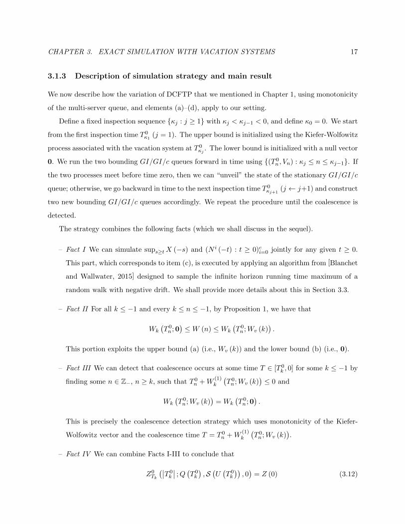
3.1.3 Description of simulation strategy and main result
We now describe how the variation of DCFTP that we mentioned in Chapter 1, using monotonicity
of the multi-server queue, and elements (a)–(d), apply to our setting.
Define a fixed inspection sequence κj : j ≥ 1 with κj < κj−1 < 0, and define κ0 = 0. We start
from the first inspection time T 0κ1 (j = 1). The upper bound is initialized using the Kiefer-Wolfowitz
process associated with the vacation system at T 0κj . The lower bound is initialized with a null vector
0. We run the two bounding GI/GI/c queues forward in time using (T 0n , Vn) : κj ≤ n ≤ κj−1. If
the two processes meet before time zero, then we can “unveil” the state of the stationary GI/GI/c
queue; otherwise, we go backward in time to the next inspection time T 0κj+1
(j ← j+1) and construct
two new bounding GI/GI/c queues accordingly. We repeat the procedure until the coalescence is
detected.
The strategy combines the following facts (which we shall discuss in the sequel).
– Fact I We can simulate sups≥tX (−s) and (N i (−t) : t ≥ 0)ci=0 jointly for any given t ≥ 0.
This part, which corresponds to item (c), is executed by applying an algorithm from [Blanchet
and Wallwater, 2015] designed to sample the infinite horizon running time maximum of a
random walk with negative drift. We shall provide more details about this in Section 3.3.
– Fact II For all k ≤ −1 and every k ≤ n ≤ −1, by Proposition 1, we have that
Wk
(T 0n ; 0
)≤W (n) ≤Wk
(T 0n ;Wv (k)
).
This portion exploits the upper bound (a) (i.e., Wv (k)) and the lower bound (b) (i.e., 0).
– Fact III We can detect that coalescence occurs at some time T ∈ [T 0k , 0] for some k ≤ −1 by
finding some n ∈ Z−, n ≥ k, such that T 0n +W
(1)k
(T 0n ;Wv (k)
)≤ 0 and
Wk
(T 0n ;Wv (k)
)= Wk
(T 0n ; 0
).
This is precisely the coalescence detection strategy which uses monotonicity of the Kiefer-
Wolfowitz vector and the coalescence time T = T 0n +W
(1)k
(T 0n ;Wv (k)
).
– Fact IV We can combine Facts I-III to conclude that
Z0Tk
(∣∣T 0k
∣∣ ;Q (T 0k
),S(U(T 0k
)), 0)
= Z (0) (3.12)
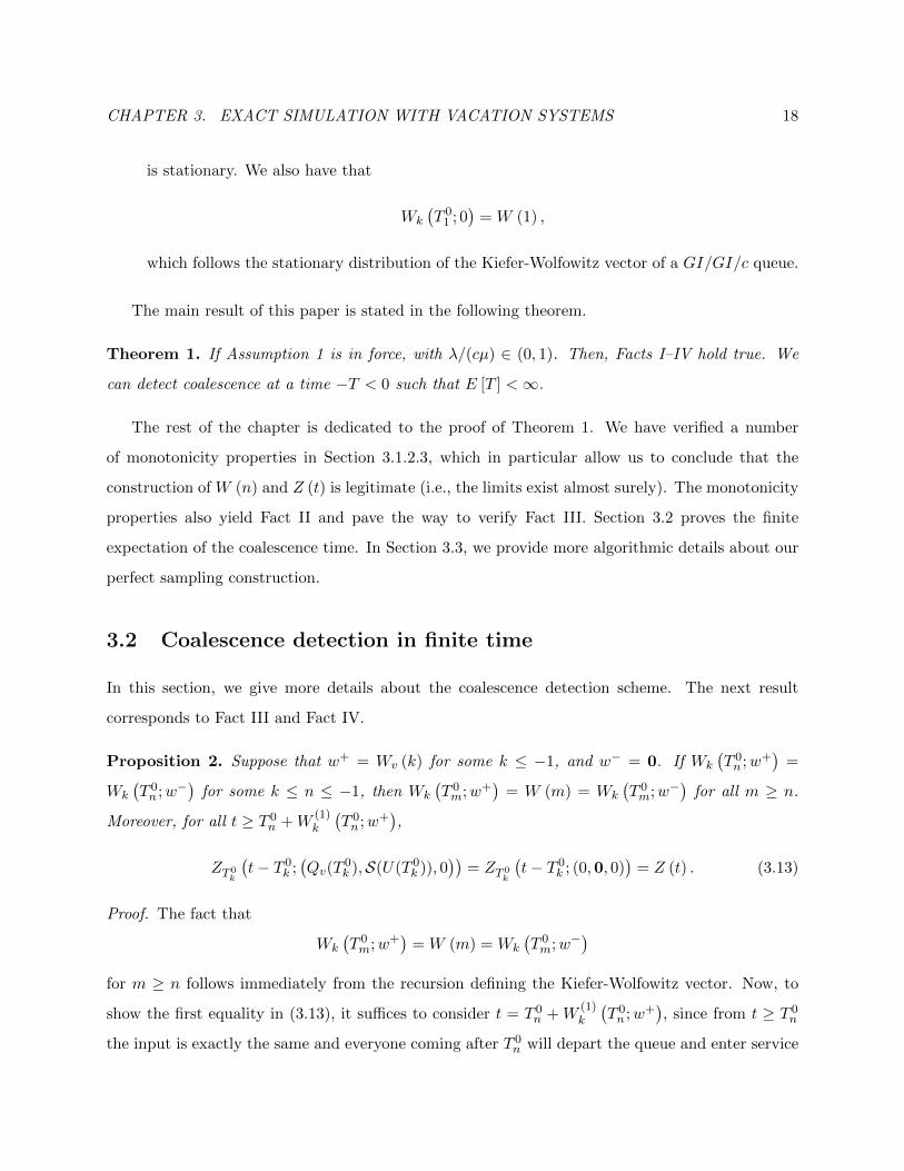
CHAPTER 3. EXACT SIMULATION WITH VACATION SYSTEMS 18
is stationary. We also have that
Wk
(T 0
1 ; 0)
= W (1) ,
which follows the stationary distribution of the Kiefer-Wolfowitz vector of a GI/GI/c queue.
The main result of this paper is stated in the following theorem.
Theorem 1. If Assumption 1 is in force, with λ/(cµ) ∈ (0, 1). Then, Facts I–IV hold true. We
can detect coalescence at a time −T < 0 such that E [T ] <∞.
The rest of the chapter is dedicated to the proof of Theorem 1. We have verified a number
of monotonicity properties in Section 3.1.2.3, which in particular allow us to conclude that the
construction of W (n) and Z (t) is legitimate (i.e., the limits exist almost surely). The monotonicity
properties also yield Fact II and pave the way to verify Fact III. Section 3.2 proves the finite
expectation of the coalescence time. In Section 3.3, we provide more algorithmic details about our
perfect sampling construction.
3.2 Coalescence detection in finite time
In this section, we give more details about the coalescence detection scheme. The next result
corresponds to Fact III and Fact IV.
Proposition 2. Suppose that w+ = Wv (k) for some k ≤ −1, and w− = 0. If Wk
(T 0n ;w+
)=
Wk
(T 0n ;w−
)for some k ≤ n ≤ −1, then Wk
(T 0m;w+
)= W (m) = Wk
(T 0m;w−
)for all m ≥ n.
Moreover, for all t ≥ T 0n +W
(1)k
(T 0n ;w+
),
ZT 0k
(t− T 0
k ;(Qv(T
0k ),S(U(T 0
k )), 0))
= ZT 0k
(t− T 0
k ; (0,0, 0))
= Z (t) . (3.13)
Proof. The fact that
Wk
(T 0m;w+
)= W (m) = Wk
(T 0m;w−
)for m ≥ n follows immediately from the recursion defining the Kiefer-Wolfowitz vector. Now, to
show the first equality in (3.13), it suffices to consider t = T 0n + W
(1)k
(T 0n ;w+
), since from t ≥ T 0
n
the input is exactly the same and everyone coming after T 0n will depart the queue and enter service

CHAPTER 3. EXACT SIMULATION WITH VACATION SYSTEMS 19
after time T 0n +W
(1)k
(T 0n ;w+
). The arrival processes (i.e., Eu (·)) clearly agree, so we just need to
verify that the queue lengths and the residual service times agree. First, note that
RT 0k(T 0n +W
(1)k
(T 0n ;w+
)− T 0
k ;(Qv(T
0k ),S(U(T 0
k )), 0))
=Wk
(T 0n ;w+
)−W (1)
k
(T 0n ;w+
)· 1
=Wk
(T 0n ;w−
)−W (1)
k
(T 0n ;w−
)· 1
=RT 0k(T 0n +W
(1)k
(T 0n ;w−
)− T 0
k ; (0,0, 0)). (3.14)
So, the residual service times of both upper and lower bound processes agree. The agreement of the
queue lengths follows from Lemma 3. Finally, the second equality in (3.13) follows from Proposition
1.
Next, we analyze properties of the coalescence time. Define
T− = supT 0k ≤ 0 : inf
T 0k≤t≤0
‖ ZT 0k
(t− T 0
k ;(Qv(T 0k
),S(U(T 0
k )), 0))
−ZT 0k
(t− T 0
k ; (0,0, 0))‖∞ = 0.
Notice that if at time T− we start an upper bound queue,
ZT− (·; (Qv(T−),S(U(T−)), 0)) ,
and a lower bound queue, ZT− (·; (0,0, 0)), they will coalesce before time 0. Thus, if we simulate
the system up to T−, we will be able to detect a coalescence. We next establish that E[|T−|] <∞.
By stationarity, we have that |T−| is equal in distribution to
T = inf
T 0k ≥ 0 : inf
0≤t≤T 0k
‖Z0 (t; (Qv(0),S(U(0)), 0))− Z0 (t; (0,0, 0))‖∞ = 0
.
Proposition 3. If E[Vn] < cE[An] for n ≥ 1 and Assumption 1 holds,
E[T ] <∞.
Proof. Define
τ = infn ≥ 1 : W1
(T 0n ;Wv (1)
)= W1
(T 0n ; 0).
By Wald’s identity, E[An] <∞, for any n ≥ 1; it suffices to show that E[τ ] <∞.

CHAPTER 3. EXACT SIMULATION WITH VACATION SYSTEMS 20
We start with an outline of the proof, which involves two main components. I) We first construct
a sequence of events which lead to the occurrence of τ . The events that we construct put constraints
on the interarrival times and service times so that we see a decreasing trend on the Kiefer-Wolfowitz
vectors. When putting a number of these events together (consecutively), the waiting time of the
upper bound system will drop to zero. We further impose the events for c more arrivals after the
waiting time drops to zero. Notice that these c arrivals do not have to wait in both the upper bound
and the lower bound systems. Thus, by the time of c-th such arrival, the two systems will have the
same set of customers with the same remaining service times. II) Based on events constructed in
I, we then split the process W1(T 0n ;Wv(1)) : n ≥ 1 into cycles where: IIa) the probability that
the desired event, which leads to coalescence, happens during each cycle is bounded from below by
a positive constant, and IIb) the expected cycle length is bounded from above by a constant. IIa
allows us to bound the number of cycles we need to check before finding τ by a geometric random
variable. Then, we apply Wald’s identity using IIb to establish an upper bound for E[τ ].
We next provide more details of the proof, which are divided into part I and II as outlined
above.
Part I We first construct the sequence of events, Ωk : k ≥ 2, which enjoys the property that if
Ωk happens, the two bounding systems would have coalesced by time of the (k + dcK/εe − 1)-th
arrival.
As E[Vn] < cE[An], for n ≥ 2, we can find m, ε > 0 such that for every n ≥ 2, the event
Hn = Vn < cm− ε, An > m is nontrivial in the sense that P (Hn) > δ for some δ > 0. Now, pick
K > cm large enough, and define, for k ≥ 2,
Ωk =W
(c)1
(T 0k ;Wv(1)
)≤ K
k+dcK/εe−1⋂n=k
Hn.
To see the coalescence of the two bounding systems, let Wk = (K,K, . . . ,K)T be a c-dimensional
vector with each element equal to K. We notice that, under Ωk,
Wk ≥W1
(T 0k ;Wv (1)
).
For n ≥ k, define Vn = cm− ε, An = m, and the (auxiliary) Kiefer-Wolfowitz sequence
Wn+1 = S((
Wn + Vne1 − An1)+).

CHAPTER 3. EXACT SIMULATION WITH VACATION SYSTEMS 21
Then, Ωk implies Vn < Vn and An > An for n ≥ k, which in turn implies
W1
(T 0n ;Wv (1)
)≤ Wn.
Moreover, under Ωk, we have
W (1)n = 0 and W (c)
n < cm for n = k + dcK/εe − c+ 1, . . . , k + dcK/εe.
Then, W(1)1
(T 0n ;Wv (1)
)= 0 and W
(c)1
(T 0n ;Wv (1)
)< cm for n = k+dcK/εe−c+1, . . . , k+dcK/εe.
This indicates that under Ωk, (1) all the arrivals between the (k + dcK/εe − c + 1)-th arrival and
the (k + dcK/εe)-th arrival (included) enter service immediately upon arrival (have zero waiting
time), and (2) the customers initially seen by the (k + dcK/εe − c + 1)-th arrival would have left
the system by the time of the (k + dcK/εe)-th arrival. The same analysis holds assuming that we
replace W1
(T 0k ;Wv (1)
)by W1
(T 0k ; 0). Therefore, by the time of the (k + dcK/εe − 1)-th arrival,
the two bounding systems would have exactly the same set of customers with exactly the same
remaining service times, which is equal to their service times minus the time elapsed since their
arrival times (since all of them start service immediately upon arrival). We also notice that since
there is no customer waiting, the sorted remaining service time at T 0k+dcK/εe−1 coincides with the
Kiefer-Wolfowitz vector Wk+dcK/εe−1.
Part II We first introduce how to split the process into cycles, which are denoted as (κi, κi+1), i ≥1. Let UK := w : w(c) ≤ K. We define
κ1 := infn ≥ 1 : W1
(T 0n ;Wv (1)
)∈ UK,
and for i ≥ 2, define
κi :=n > κi−1 + dcK/εe − 1 : W1(T 0
n ;Wv(1)) ∈ UK.
We denote Θi =⋂κi+dcK/εe−1n=κi
Hn for i ≥ 1. We next show that the event Θi happens during the
i-th cycle with positive probability. Since P (Hn) > δ, P (Θi) ≥ δdcK/εe > 0. Let N denote the first
i for which Θi occurs. Then, N is stochastically bounded by a geometric random variable with
probability of success δdcK/εe. In particular, E[N ] ≤ δ−dcK/εe <∞.
We next show that E[κi+1 − κi] is bounded using the standard Lyapunov argument. Under
Assumption 1 and λ < cµ, W1
(T 0n ;w (1)
): n ≥ 1 for any fixed initial condition w(1) is a positive

CHAPTER 3. EXACT SIMULATION WITH VACATION SYSTEMS 22
recurrent Harris chain [Asmussen, 2003]. Under Assumption 1, we also have that (Qv(t) : t ∈(−∞,∞)) is a well-defined process with E[Qv(t)] < ∞ (see the random-walk bound in (3.18)).
Thus,
E
[c∑i=1
W (i)v (1)
]<∞.
Consider the Lyapunov function g(W ) = W (c), i.e., g(W ) ≥ 0 and g(W ) → ∞ as ||W || → ∞.
Then, for K large enough, as λ < cµ, we can find δ ∈ (0, c/λ− 1/µ) such that
E[g(W1(T 0
c+1, w(1))]≤ g(w(1))− δ for w(1) 6∈ UK . (3.15)
We also have
E[g(W1(T 0
c+1, w(1))]≤ K + c/µ for w(1) ∈ UK .
Then, by Theorem 2 in [Foss and Konstantopoulos, 2006], E[κ1] < ∞ and we can find a constant
M > 0 such that E[κi− κi−1] < M for i ≥ 2. We comment that here we need to look c steps ahead
to identify the downward drift in (3.15), Thus, we use a general version of Lyapunov argument
developed in [Foss and Konstantopoulos, 2006].
Lastly, by Wald’s identity we have (setting κ0 = 0) that
E[τ ] ≤ E[κN ] + dcK/εe − 1
= E
N∑i=1
(κi − κi−1) + dcK/εe − 1
≤ E[N ]×M + E[κ1] + dcK/εe − 1 <∞.
Remark 1. Following the proof, we can also conclude that the number of “activities” (either
vacations or services) to simulate in the vacation system, denoted as NV , is also finite in expectation.
Since coalescence is detected by the τ -th arrival, we only need to simulate the vacation system
forward in time from time 0 until we are able to extract the first Qv(0)+τ service time requirements
to match the customers waiting in queue at time 0 and the arrivals from time 0 to coalescence time
T .
For any m′ <∞ such that E[V ∧m′] > 0, we let N i(t), i = 1, . . . , c, denote the counting process
corresponding to the i-th “truncated” vacation process with independent activity times capped by

CHAPTER 3. EXACT SIMULATION WITH VACATION SYSTEMS 23
m′, i.e., V ∧m′. Following a standard argument as in the proof of Ward’s identity in [Asmussen,
2003], a loose upper bound for E[Nv] is given by
E [NV ] ≤c∑i=1
E[N i(T ) + 1
]+ E [Qv(0) + τ ]
≤c∑i=1
E[N i(T ) + 1
]+ E [Qv(0)] + E [τ ]
≤ c · E [T ] +m′
E [V ∧m′] + E [Qv(0)] + E [τ ] <∞.
3.3 Simulation procedure
In this section, we first address the validity of Fact I, namely, that we can simulate the vacation
system backward in time, jointly withT in : m ≤ n ≤ −1
for 0 ≤ i ≤ c, for any m ∈ Z−.
Let Ge(·) = λ∫ ·
0 G(x)dx and Fe(·) = µ∫ ·
0 F (x)dx denote equilibrium CDFs of the interarrival
time and service time distributions, respectively. We first notice that simulating the stationary
arrival processT 0n : n ≤ −1
and stationary service/vacation completion process
T in : n ≤ −1
for each 1 ≤ i ≤ c is straightforward by the reversibility of T in for 0 ≤ i ≤ c. Specifically, we can
simulate the renewal arrival process forward in time from time 0 with the first interarrival time
following Ge and subsequent interarrival times following G. We then set T 0−k = −T 0
k for all k ≥ 1.
Likewise, we can also simulate the service/vacation process of server i, for i = 1, . . . , c, forward
in time from time 0 with the first service/vacation initiation time following Fe and subsequent
service/vacation time requirements distributed as F . Let T ik, k ≥ 1, denote the k-th service/vacation
initiation time of server i counting forward in time. Then, we set T i−k = −T ik.Similarly, we have the equality in distribution, for all t ≥ 0 (jointly),
X (−t) d= X (t) ;
therefore, we have from (3.2) that the following equality in distribution holds for all t ≥ 0 (jointly):
Qv(−t) d= sup
s≥tX (s)−X (t) .
The challenge in simulating Qv(−t) involves sampling M(t) = maxs≥tX(s) jointly with X(t)
during any time interval of the form [0, T ] for T > 0. The rest of the section is devoted to solve
this challenge.
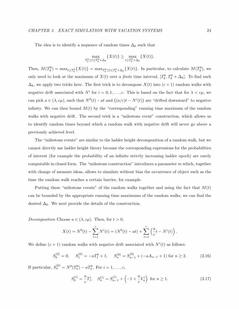
CHAPTER 3. EXACT SIMULATION WITH VACATION SYSTEMS 24
The idea is to identify a sequence of random times ∆k such that
maxT 0k≤t≤T
0k+∆k
X(t) ≥ maxt≥T 0
k+∆k
X(t).
Then, M(T 0k ) = maxt≥T 0
kX(t) = maxT 0
k≤t≤T0k+∆k
X(t). In particular, to calculate M(T 0k ), we
only need to look at the maximum of X(t) over a finite time interval, [T 0k , T
0k + ∆k]. To find such
∆k, we apply two tricks here. The first trick is to decompose X(t) into (c+ 1) random walks with
negative drift associated with N i for i = 0, 1, . . . , c. This is based on the fact that for λ < cµ, we
can pick a ∈ (λ, cµ), such that N0(t)− at and((a/c)t−N i(t)
)are “drifted downward” to negative
infinity. We can then bound M(t) by the “corresponding” running time maximum of the random
walks with negative drift. The second trick is a “milestone event” construction, which allows us
to identify random times beyond which a random walk with negative drift will never go above a
previously achieved level.
The “milestone events” are similar to the ladder height decomposition of a random walk, but we
cannot directly use ladder height theory because the corresponding expressions for the probabilities
of interest (for example the probability of an infinite strictly increasing ladder epoch) are rarely
computable in closed form. The “milestone construction” introduces a parameter m which, together
with change of measure ideas, allows to simulate without bias the occurrence of object such as the
time the random walk reaches a certain barrier, for example.
Putting these “milestone events” of the random walks together and using the fact that M(t)
can be bounded by the appropriate running time maximums of the random walks, we can find the
desired ∆k. We next provide the details of the construction.
Decomposition Choose a ∈ (λ, cµ). Then, for t > 0,
X(t) = N0(t)−c∑i=1
N i(t) = (N0(t)− at) +c∑i=1
(act−N i(t)
).
We define (c+ 1) random walks with negative drift associated with N i(t) as follows:
S(0)0 = 0, S
(0)1 = −aT 0
1 + 1, S(0)n = S
(0)n−1 + (−aAn−1 + 1) for n ≥ 2. (3.16)
If particular, S(0)n = N0(T 0
n)− aT 0n . For i = 1, . . . , c,
S(i)0 =
a
cT i1, S(i)
n = S(i)n−1 +
(−1 +
a
cV in
)for n ≥ 1. (3.17)

CHAPTER 3. EXACT SIMULATION WITH VACATION SYSTEMS 25
Here, S(i)n = N i(T in−) − aT in. Figure 3.2 plots the relationship between N0(t) − at : t ≥ 0 and
S(0)n : n ≥ 0, and the relationship between ac t−N i(t) : t ≥ 0 and S(i)
n : n ≥ 0 for i = 1, . . . , c.
In particular, we notice from Figure 3.2 that
maxs≥t
N0(s)− as
= max
N0(t)− at, max
n≥N0(t)+1S(0)
n ≤ max
n≥N0(t)
S(0)n
,
and for i = 1, . . . , c,
maxs≥t
acs−N i(s)
= max
n≥N i(t−)
S(i)n
≤ max
n≥(N i(t)−1)+
S(i)n
.
N00 (t)− at
t
S1(0)
S2(0)
S3(0)
S4(0)
S0(0)
0
(a)
act − N0
i (t)
tS1(i )
S2(i )
S3(i )
S4(i )
S0(i )
0
(b)
Figure 3.2: The relationship between the renewal processes and the random walks (a) N0(t)− atand S
(0)n (b) (a/c)t−N i(t) and S
(i)n
We then notice that, for any given T ,
M(T ) = maxt≥TX(t) = max
t≥T
(N0(t)− at) +
c∑i=1
(act−N i(t)
)
≤ maxt≥T
N0(t)− at
+
c∑i=1
maxt≥T
act−N i(t)
≤ max
n≥N0(T )
S(0)n
+
c∑i=1
maxn≥N i(T )−1
S(i)n
. (3.18)
Milestone construction We use the “milestone events” construction to generate the (c+ 1) random
walks with negative drift, S(i), together with their running time maxima, M(i)k := maxn≥kS(i)
n ,k ≥ 0, i = 0, 1, . . . c. This construction is introduced in [Blanchet and Sigman, 2011; Blanchet and
Wallwater, 2015], and we shall provide a brief overview here.

CHAPTER 3. EXACT SIMULATION WITH VACATION SYSTEMS 26
Fix m > 0 and L ≥ 1 such that P (m < M(i)0 ≤ (L+ 1)m) > 0 for i = 0, . . . , c. The values of m
and L do not seem to have significant impact on algorithm performance, as long as they are chosen
to be small. In our numerical implementations, we choose m = 1 and L = 3.
For each random walk S(i)n : n ≥ 0, i = 0, 1, . . . , c, we shall define a sequence of downward
and upward “milestone events”, which we denoted as Φij and Υi
j , respectively, for j ≥ 0 as follows:
Φi0 := 0, Υi
0 := 0,
and for j ≥ 1,
Φij := inf
n ≥ Υi
j−1I(Υij−1 <∞) ∨ Φi
j−1 : S(i)n < S
(i)
Φij−1− Lm
,
Υij := inf
n ≥ Φi
j : S(i)n > S
(i)
Φij+m
.
Notice that P (Φij <∞) = 1 while P (Υi
j <∞) < 1, as the random walks have negative drift. In fact,
under Assumption 1, Proposition 2.1 in [Blanchet and Wallwater, 2015] shows P (Υij =∞, i.o.) = 1.
We observe that when the event Υij =∞ happens, we know that the random walk will never go
above S(i)
Φij+m beyond Φi
j . This important observation allows us to find the running time maximum
M(i)k . In particular, let Φi
k∗ denote the first downward milestone at or after step k, and let Φik∗∗ be
the first downward milestone after Φ0k∗ with Υi
k∗∗ = ∞. Then, after step Φik∗∗, the random walk
S(i) will never go above the level S(i)
Φ0k∗∗
+m, and S(i)
Φ0k∗∗
+m < S(i)
Φ0k∗− Lm+m ≤ S(i)
Φik∗. Therefore,
M(i)k = maxn≥kS(i)
n = maxk≤n≤Φik∗∗S(i)
n , i.e., we just need to find the maximum value of the
random walk between step k and step Φik∗∗. Figure 3.3 provides a pictorial explanation of the
construction.
We are now ready to use the milestone events across the (c + 1) random walks to identify ∆k
associated with each T 0k (k ≥ 1), such that N i(T 0
k ) ≥ 1 for i = 1, . . . , c. Define
Λ0k := min
j≥1
Φ0j > N0(T 0
k ) : S(0)
Φ0j≤ S(0)
N0(T 0k )−m,Υ0
j =∞, (3.19)
and, for i = 1, · · · , c,
Λik := minj≥1
Φij > N i(T 0
k )− 1 : S(i)
Φij≤ S(i)
N i(T 0k )−1
−m,Υij =∞
. (3.20)

CHAPTER 3. EXACT SIMULATION WITH VACATION SYSTEMS 27
1
2
3
4
5
6
7
8
9
0
1 2 3 4 5 6 7 8 9 10 11
S(0)n
Figure 3.3: This figure plots a realization of the sample path S(0)n : 0 ≤ n ≤ 11. Here we set m = 1
and L = 3. Then, Φ01 = 3, Υ0
1 = 4, Φ02 = 7. If Υ0
2 = ∞, then for n ≥ 7, S(0)n will stay below the
level S(0)7 +m, which is demonstrated by the bold dashed line. Thus, M
(0)2 = maxn≥2S(0)
n = S(0)2
by only comparing the random walk values between step 2 and step 7.

CHAPTER 3. EXACT SIMULATION WITH VACATION SYSTEMS 28
In particular, the random walk S(i)n : n ≥ 0 will never go above the level S
(i)
Λik+ m for n ≥ Λik,
i = 0, . . . , c. Let
∆k := max
T 0
Λ0k, max
1≤i≤c
T iΛik+1
− T 0
k , (3.21)
Since N0(T 0k + ∆k
)≥ Λ0
k and N i(T 0k + ∆k)− 1 ≥ Λik for i = 1, · · · , c,
maxn≥N0(T 0
k+∆k)
S(0)n
≤ S(0)
Λ0k
+m and maxn≥N i(T 0
k+∆k)−1
S(i)n
≤ S(i)
Λik+m.
Therefore,
maxt≥T 0
k+∆k
X(t) ≤ maxn≥N0(T 0
k+∆k)
S(0)n
+
c∑i=1
maxn≥N i(T 0
k+∆k)−1
S(i)n
≤ S
(0)
Λ0k
+m+c∑i=1
(S
(i)
Λik+m
)≤ S
(0)
N0(T 0k )
+c∑i=1
S(i)
N i(T 0k )−1
≤ N0(T 0k )− aT 0
k +c∑i=1
(acT 0k −N i(T 0
k ))
= X(T 0k ) ≤ max
T 0k≤t≤T
0k+∆k
X(t).
Under Assumption 1, the time it takes to find ∆k using the “milestone” construction has finite
expectation (Theorem 2.2 in [Blanchet and Wallwater, 2015]). We shall provide the algorithmic
details to generate the random walk with negative drift together with the “milestone” events for
the light-tailed case in Section 3.3.1 to demonstrate the basic idea. The general case can be found
in [Blanchet and Wallwater, 2015]. We also provide the algorithm to match the service time
requirements to the customers in vacation system between two consecutive inspection times in
Section 3.3.2. Lastly, the exact simulation algorithm of GI/GI/c queue is summarized in Section
3.3.3.
3.3.1 Simulate a random walk with negative drift jointly with “milestone”
events
To demonstrate the basic idea, we work with a generic random walk with negative drift Sn :=
Sn−1 + Xn, for n ≥ 0, with S0 given. We also impose the light-tail assumption on Xn, i.e., there
exist θ > 0 such that E[exp(θXn)] <∞. Let

CHAPTER 3. EXACT SIMULATION WITH VACATION SYSTEMS 29
Φ0 := 0, Υ0 := 0,
and, for j ≥ 1,
Φj := infn ≥ Υj−1I(Υj−1 <∞) ∨ Φj−1 : Sn < SΦj−1 − Lm
Υj := inf
n ≥ Φj : Sn > SΦj +m
.
We also denote τm = infn ≥ 0 : Sn > m,S0 = 0. Notice that P (Υj =∞) = P (τm =∞) > 0.
Sampling Φj is straightforward. We just sample the random walk, Sn, until Sn < SΦj−1 − Lm.
Sampling Υj and the path conditional on Υj < ∞ requires more advanced simulation techniques,
as P (Υj = ∞) > 0. In particular, we use the exponential tilting idea discussed in [Asmussen,
2003]. Let ψX(θ) = logE [exp(θXn)] be the log moment generating function of Xn, then we have
E[Xn] = ψ′X(0) < 0 and V ar(Xn) = ψ′′X(0) > 0. By the convexity of ψX(·), we can always find
η > 0 with ψX(η) = 0 and ψ′X(η) ∈ (0,∞). Hence, we can define a new measure Pη based on
exponential tilting so thatdPηdP
(Xn) = exp(ηXn).
Under Pη, Sn is a random walk with positive drift ψ′X(η). Thus Pη(τm < ∞) = 1. By our choice
of η, we also have P (τm < ∞) = Eη exp(−ηSτm). In implementation, we shall we generate the
path Sn under Pη until τm and check whether U ≤ exp(−ηSτm)), where U is a uniform random
variable independent of everything. If U ≤ exp(−ηSτm)), we claim that τm < ∞ and accept the
path (Sn : n ≤ τm) as the path of the random walk conditional on τm <∞.
The algorithm to sample the random walk together with the milestone events goes as follows.
Throughout this thesis, “sample” in the pseudocode means sampling independently from everything
that has already been sampled.
Algorithm RWS: Sample a random walk with negative drift until stopping criteria are met
Input: L, m, S0, · · · , Sn, Φ0, · · · ,Φj, Υ0, · · · ,Υj and stopping criteria H.
(Note that n = Φj if Υj = ∞, and n = Υj otherwise. If there is no previous simulated partial
random walk, then we initialize n = 0, j = 0, Φ0 = 0, Υ0 = 0, and S0 as needed.)
1. While the stopping criteria H are not satisfied, set j ← j + 1.

CHAPTER 3. EXACT SIMULATION WITH VACATION SYSTEMS 30
(a) (Downward milestone simulation)
Sample Sk : n + 1 ≤ k ≤ Φj under the nominal measure, i.e., generate the random
walk until Sn < SΦj−1 − Lm. Update n = Φj .
(b) (Upward milestone simulation)
Sample S1, · · · , Sτm from the tilted measure Pη(·). Sample U ∼ Uniform[0,1]. If U ≤exp
(−ηSτm
), set Υj = n+τm, Sn+k = Sn+Sk for k = 1, · · · , τm and update n← n+τm;
otherwise set Υj =∞.
2. Output updated S0, · · · , Sn, Φ0, · · · ,Φj and Υ0, · · · ,Υj.
3.3.2 Simulate the vacation system between inspection times
To summarize our discussion above, in this section, we provide the pseudocode for generating the
vacation system between the inspection time T 0κl
and T 0κl+1
, for l ≥ 0, κ0 = 0, and κl+1 < κl.
Algorithm VSS: Sample vacation system between T 0κl
and T 0κl−1
, and extract corresponding service
times
Input: m, L, κl, κl−1, S(i)0 , · · · , S(i)
ni , Φi0, · · · ,Φi
ji, Υi
0, · · · ,Υiji for i = 0, 1, · · · , c.
1. Apply Algorithm RWS to further sample S(0) with the stopping criteria H being n0 ≥ |κl|.Then, find T 0
|κl|.
2. Apply Algorithm RWS to further sample S(0) with the stopping criteria H being n0 = Λ0|κl|,
with Λ0|κl| defined in Eq. (3.19).
3. For i = 1, · · · , c, apply Algorithm RWS to further sample S(i) until the stopping criteria Hbeing ni = Λi|κl|, with Λi|κl| defined in Eq. (3.20).
4. Compute ∆|κl| as defined in Eq. (3.21). For i = 0, 1, · · · , c, apply Algorithm RWS to further
sample S(i) with the stopping criteria H being T ini ≥ T 0|κl| + ∆|κl|.
5. Construct the backward renewal processes N i(t) : T 0κl− ∆|κl| ≤ t ≤ 0 using S(i)
n : 0 ≤n ≤ ni for i = 0, 1, · · · , c. In particular, we shall set T i−n = −T in. Then, construct X(t) =
N0(t)−∑ci=1N
i(t) for t ∈ [T 0κl−∆|κl|, 0].

CHAPTER 3. EXACT SIMULATION WITH VACATION SYSTEMS 31
6. Set M(T 0κl
) = maxT 0κl−∆|κl|≤t≤T
0κlX(t) and then compute Qv(T
0κl
) = M(T 0κl
) − X(T 0κl
) to
be the number of people waiting in the queue at time T 0κl
. The remaining activity times are
U i(T 0κl
), for i = 1, · · · , c.
7. If Qv(T0κl
) > 1, then for 1 ≤ j ≤ Qv(T0κl
) − 1, the j-th people waiting in queue arrive at
time T 0κl−Qv(T 0
κl)+j . Let Dj = inft ≥ 0 : j =
∑ci=1 σ
iT 0κl
(t), then extract Vκl−Qv(T 0κl
)+j =∑ci=1 V
iN i(T 0
κl+Dj)
dN i(T 0κl
+ Dj) as his service time.
8. For κl ≤ n ≤ −1, use Eq. (3.3) to extract their service times Vκl , · · · , V−1.
9. Output
(a) service times of the people waiting in queue at time T 0κl
(excluding the arrival at T 0κl
), i.e.,
null if Qv(T0κl
) = 1 and (Vκl−Qv(T 0κl
)+1, · · · , Vκl−1) in the order of arrivals if Qv(T0κl
) > 1.
(b) matched arrival times and service times(T 0j , Vj
): κl ≤ j ≤ −1
in the order of arrival.
(c) updated random walks S(i)0 , · · · , S(i)
ni with updated milestone events Φi0, · · · ,Φi
ji,
Υi0, · · · ,Υi
ji for i = 0, 1, · · · , c.
3.3.3 Overall exact simulation procedure
In this section, we provide the overall pseudocode for our exact simulation algorithm.
Algortihm PS: sample stationary GI/GI/c queue at time 0
Input: m, L, F , G, c
1. For i = 0, 1, · · · , c, initiate Φi0 = Υi
0 = 0, and S(i)0 as defined in Eqs. (3.16, 3.17).
2. Set κ0 = 0, κ1 = −10, l = 1.
3. (a) Apply Algorithm VSS to sample vacation system between T 0κl
and T 0κl−1
, and extract
corresponding service times.
(b) Start two GI/GI/c queues, both from T 0κl
, one initialized with
(Qv(T
0κl
),S(U(T 0κl
)), 0)

CHAPTER 3. EXACT SIMULATION WITH VACATION SYSTEMS 32
and the other initialized with 0. Evolve the two queues forward in time until time 0 and
calculate
C = minκl≤j≤−1
||ZT 0κl
(T 0j − T 0
κl;(Qv(T
0κl
),S(U(T 0κl
)), 0))
− ZT 0κl
(T 0j − T 0
κl; 0)||∞.
4. If C = 0, output Z(0) = ZT 0κl
(|T 0κl|; 0). Otherwise (C > 0), set l ← l + 1, κl = 2κl−1, then
go back to Step 3.
3.4 Numerical experiments
As a sanity check, we have implemented our MATLAB code in the case of an
Erlang (k1, λ) /Erlang (k2, µ) /c queue.
Firstly, in the context of the M/M/c queue, which is a special case of
Erlang(k1, λ)/Erlang(k2, µ)/c when k1 = k2 = 1 and whose stationary distribution can be
computed in closed form, we have compared the theoretical distribution to the empirical distri-
bution of the number of customers in the system at stationarity. The empirical distribution is
produced from a large number of runs using our perfect simulation algorithm. Figure 3.4 shows
a comparison of these distributions when λ = 3, µ = 2 and c = 2. Grey bars show the empirical
result of 5000 draws using our perfect simulation algorithm, and black bars show the theoretical
distribution of the number of customers in the system. The two are very close to each other.
Following [Connor and Kendall, 2015], we test the goodness of fit using a Pearson’s chi-squared
test; under the null hypothesis, the empirical histogram converges to theoretical distribution as
the sample size increases. The test yields a p-value equal to 0.6806, indicating close agreement
(i.e., we can not reject the null hypothesis). Similarly, Figure 3.5 provides another comparison
with a different set of parameters, λ = 10, µ = 2, c = 10, with a p-value being 0.6454 from the
chi-squared test.
Also, for a general Erlang(k1, λ)/Erlang(k2, µ)/c queue (k1 > 1, k2 > 1) when traffic intensity
ρ = (λ1k2) / (cλ2k1) = 0.9, we have compared the empirical distribution obtained from simulation
with the numerical results (with precision at least 10−4) provided in Table III of [Hillier and Lo,
1971]. Figure 3.6 shows the comparison for an E3/E2/5 queue with ρ = 0.9. We observe that the

CHAPTER 3. EXACT SIMULATION WITH VACATION SYSTEMS 33
0 5 10 15 20 25 300
0.05
0.1
0.15
0.2
0.25Number of Customers for an M/M/c queue in equilibrium with lambda = 3, mu = 2, c = 2 (5000 draws)
Perfect SimulationTheoretical
Figure 3.4: Number of customers for an M/M/c queue in stationarity when λ = 3, µ = 2 and
c = 2.
two histograms are very close to each other. A Pearson’s chi-squared test between the simulated
distribution and the numerical one gives a p-value of 0.6815.
Next, we run numerical experiments in M/M/c case to see how the running time of our al-
gorithm, measured by mean coalescence time of two bounding systems, scales as the number of
servers grows and the traffic intensity ρ changes. Starting from time 0, the upper bound queue
has its queue length sampled from the theoretical distribution of an M/M/c vacation system and
all servers busy with remaining service times drawn from the equilibrium distribution of the ser-
vice/vacation time; and the lower bound queue is empty. Then, we run both the upper bound and
lower bound queues forward in time with the same stream of arrival times and service requirements
until they coalescence. Table 3.1 shows the estimated mean coalescence time, E[T ], based on 5000
iid samples, for different system scales in the quality-driven regime (QD). We observe that E[T ]
does not increase much as the system scale parameter, s, grows. Table 3.2 shows similar results for
the quality-and-efficiency driven operating regime (QED). In this case, E[T ] increases at a faster
rate with s than the QD case, but the magnitude of increment is still not significant.
Finally we run a numerical experiment in the M/M/c case aiming to test how computational
complexity of our algorithm changes with traffic intensity, ρ = λ/(cµ). Here, we define the com-
putational complexity as the total number of renewals (including arrivals and services/vacations)

CHAPTER 3. EXACT SIMULATION WITH VACATION SYSTEMS 34
0 5 10 15 20 25 300
0.02
0.04
0.06
0.08
0.1
0.12
0.14
0.16
0.18Number of Customers for an M/M/c queue in equilibrium with lambda = 10, mu = 2, c = 10 (5000 draws)
Perfect SimulationTheoretical
Figure 3.5: Number of customers for an M/M/c queue in stationarity when λ = 10, µ = 2 and
c = 10.
0 5 10 15 20 25 300
0.05
0.1
0.15Number of Customers for an E3/E2/5 queue in equilibrium with rho=0.9 (5000 draws)
Perfect SimulationNumerical Table
Figure 3.6: Number of customers for an Erlang(k1, λ)/Erlang(k2, µ)/c queue in stationarity when
k1 = 3, λ = 4.5, k2 = 2, µ = 2/3, c = 5 and ρ = 0.9.

CHAPTER 3. EXACT SIMULATION WITH VACATION SYSTEMS 35
Table 3.1: Simulation estimates for the mean coalescence time of M/M/c queue (QD)
(λs = s, cs = 1.2s, µ = 1)
s Mean 95% confidence interval
100 6.4212 [6.2902, 6.5522]
500 7.0641 [6.9848, 7.1434]
1000 7.7465 [7.6667, 7.8263]
Table 3.2: Simulation estimates for the mean coalescence time of M/M/c queue (QED)
(λs = s, cs = s+ 2√s, µ = 1)
s Mean 95% confidence interval
100 6.5074 [6.3771, 6.6377]
500 8.5896 [8.4361, 8.7431]
1000 9.4723 [9.3041, 9.6405]
the algorithm samples in total to find the coalescence time. We expect the complexity to scale like
(c + 1)(1 − ρ)−2E[T (ρ)], where (c + 1) is the number of renewal processes we need to simulate,
(1−ρ)−2 is on average the amount of renewals we need to sample to find its running time maximum
for each renewal process, and E[T (ρ)] is the mean coalescence time when the traffic intensity is
ρ. Table 3.3 summarizes our numeral results, based 5000 independent runs of the algorithm for
each ρ. We run the coalescence check at κ = 10 × 2k, for k = 1, 2, . . . , until we find the coales-
cence. We observe that as ρ increase, the computational complexity increases significantly, but
when multiplied by (1 − ρ)2, the resulting products are of about the same magnitude – up to a
factor proportional to λ, given that the number of arrivals scales as λ per unit time. Therefore, the
main scaling parameter for the complexity here is (1− ρ)−2. Notice that if we simulate the system
forward in time from empty, it also took around O((1− ρ)−2
)arrivals to get close to stationary.

CHAPTER 3. EXACT SIMULATION WITH VACATION SYSTEMS 36
Table 3.3: Simulation result for computational complexities with varying traffic intensities
M/M/c queue with fixed µ = 5 and c = 2
λ traffic
intensity (ρ)
mean number of
renewals sampled
mean index of successful
inspection time
mean number of renewals
sampled × (1− ρ)2
5 0.5 225.6670 11.7780 56.4168
6 0.6 377.0050 14.7780 60.3208
7 0.7 764.3714 21.9800 68.7934
8 0.8 2,181.3452 44.2320 87.2538
9 0.9 12,162.6158 161.0840 121.6262

CHAPTER 4. EXACT SIMULATION WITH RANDOM ASSIGNMENT 37
Chapter 4
Exact Simulation with Random
Assignment
We give our second set of exact simulation algorithms, which utilizes dominated coupling from the
past (DCFTP) protocol and the random assignment (RA) discipline, in this chapter. In Section
4.1, we give some theoretical background of multi-server queues under FIFO and RA, and establish
the dominance relationship of workload between these two different service disciplines. In Section
4.2, we describe our simulation strategies and the main theoretic result. In Section 4.3, we provide
the numerical experiments results for sanity check and performance comparison. In Sections 4.4
and 4.5, we extend the developed algorithm to perform perfect sampling for various other queueing
settings. Detailed simulation algorithm steps and the proof of the main technical result are provided
in Appendix B.
4.1 The FIFO and RA GI/GI/c model
4.1.1 The FIFO GI/GI/c model
In what follows, as input to a c-server in parallel multi-server queue, we have iid service times
Vn : n ≥ 0 distributed as F (x) = P (V ≤ x), x ≥ 0, with finite and non-zero mean 0 < E[V ] =
1/µ < ∞. Independently, the arrival times tn : n ≥ 0 (t0 = 0) to the model form a renewal
process with iid interarrival times An = tn+1 − tn, n ≥ 0 distributed as G(x) = P (A ≤ x), x ≥ 0,

CHAPTER 4. EXACT SIMULATION WITH RANDOM ASSIGNMENT 38
and finite non-zero arrival rate 0 < λ = E[A]−1 < ∞. The FIFO GI/GI/c model has only one
queue (line), and we let Wn = (Wn(1), . . . ,Wn(c))T denote the Kiefer-Wolfowitz workload vector
(see, for example, Page 341 in Chapter 12 of [Asmussen, 2003]). It satisfies the recursion
Wn+1 = S (Wn + Vne1 −An1)+ , n ≥ 0, (4.1)
where e1 = (1, 0, . . . 0)T , 1 = (1, 1, . . . , 1)T , S places a vector in ascending order, and + takes the
positive part of each coordinate, as we mentioned earlier in Eq. (3.4). Let Cn denote the nth
arriving customer. For i = 1, . . . , c, Wn(i) is the waiting time of Cn if he decides to enter service
immediately after there are at least i servers available once he reaches the head of the queue, i.e.,
Dn = Wn(1) is the customer delay in queue (line) of Cn. Recursion (4.1) defines a Markov chain
due to the given iid assumptions.
With stability condition ρ = λ/(cµ) < 1, it is well known that Wn converges in distribution as
n → ∞ to a proper stationary distribution. Let π denote this stationary distribution. Again, our
main objective is to provide a simulation algorithm for sampling exactly from π.
4.1.2 The RA GI/GI/c model
Given a c-server queueing system, the random assignment model (RA) is the case when each of the
c servers forms its own FIFO single-server queue, and each arrival to the system, independent of
the past, randomly chooses queue i to join with equal probability 1/c, 1 ≤ i ≤ c. In the GI/GI/c
case, we refer to this as the RA GI/GI/c model. The following is a special case of Lemma 1.3, Page
342 in [Asmussen, 2003]. Such results and others even more general are based on [Wolff, 1987],
[Foss, 1980], and [Foss and Chernova, 2001].
Lemma 4. Let QF (t) denote total number of customers in system at time t ≥ 0 for the FIFO
GI/GI/c model, and let QRA(t) denote total number of customers in system at time t ≥ 0 for the
corresponding RA GI/GI/c model in which both models are initially empty and fed with exactly the
same input of renewal arrivals tn : n ≥ 0 and iid service times Vn : n ≥ 0. Assume further that
for both models the service times are used by the servers in the order in which service initiations
occur (Vn is the service time used for the n-th such initiation). Then,
P (QF (t) ≤ QRA(t), for all t ≥ 0) = 1. (4.2)

CHAPTER 4. EXACT SIMULATION WITH RANDOM ASSIGNMENT 39
The importance of Lemma 4 is that it allows us to jointly simulate versions of the two stochastic
processes QF (t) : t ≥ 0 and QRA(t) : t ≥ 0 while achieving a coupling such that (4.2) holds. In
particular, whenever an arrival finds the RA model empty, the FIFO model is found empty as well.
(But we need to impose further conditions if we wish to ensure that indeed the RA GI/GI/c queue
will empty with certainty.) Letting time t be sampled at arrival times of customers, tn : n ≥ 0,we thus also have
P (QF (tn−) ≤ QRA(tn−), for all n ≥ 0) = 1. (4.3)
In other words, the total number in system as found by the n-th arrival is sample-path ordered
as well. Note that for the FIFO model, the n-th arriving customer Cn initiates the n-th service
since FIFO means “First-In-Queue-First-Out-of-Queue” where by “queue” we mean the line before
entering service. This means that for the FIFO model we can attach Vn to Cn upon arrival if we
so wish when applying Lemma 4. For the RA model, however, customers are not served in the
order they arrive. For example, consider c = 2 servers (system initially empty) and suppose C1 is
assigned to server 1 with service time V1, and C2 also is assigned to server 1 (before C1 departs)
with service time V2. Meanwhile, before C1 departs, suppose C3 arrives and is assigned to the
empty server 2 with service time V3. Then, V3 is used for the second service initiation. For RA, the
service times in the order of initiation are a random permutation of the originally assigned Vn.To use Lemma 4, it is crucial to simply let the servers hand out service times one at a time
when they are needed for a service initiation. Thus, customers waiting in a queue before starting
service do not have a service time assigned until they enter service. In simulation terminology, this
amounts to generating the service times in order of when they are needed.
One disadvantage of generating service times only when they are needed, is that it then does
not allow workload1 to be defined; only the amount of work in service. To get around this if need
be, one can simply generate service times upon arrival of customers, and give them to the servers
to be used in the order of service initiation. The point is that when Cn arrives, the total work in
system jumps up by the amount Vn. But Vn is not assigned to Cn, it is assigned (perhaps later) to
which ever customer initiates the n-th service. This allows Lemma 4 to hold true for total amount
1Workload (total) at any time t is defined as the sum of all whole and remaining service times in the system at
time t.

CHAPTER 4. EXACT SIMULATION WITH RANDOM ASSIGNMENT 40
of work in the system: If we let νF (t) : t ≥ 0 and νRA(t) : t ≥ 0 denote total workload in the
two models with the service times used in the manner just explained, then in addition to Lemma 4
we have
P (νF (t) ≤ νRA(t), for all t ≥ 0) = 1, (4.4)
P (νF (tn−) ≤ νRA(tn−), for all n ≥ 0) = 1. (4.5)
It is important, however, to note that what one can’t do is define workload at the individual
server i by doing this, because that forces us to assign Vn to Cn so that workload at the server that
Cn attends (i say) jumps by Vn and Cn enters service using Vn; that destroys the proper coupling
needed to obtain Lemma 4. We can only handle the total (sum over all c nodes) workload. In the
present chapter, our use of Lemma 4 is via a kind of reversal:
Lemma 5. Let V ′n be an iid sequence of service times distributed as F , and assign V ′n to Cn in
the RA model. Define Vn as the service time used in the n-th service initiation. Then, Vn is also
iid distributed as F .
Proof. The key is noting that we are re-ordering based only on the order in which service times
begin being used, not when they are completed (which would thus introduce a bias). The service
time chosen for the next initiation either enters service immediately (e.g., is one that is routed to
an empty queue by an arriving customer) or is chosen from among those waiting in lines, and all
those waiting are iid distributed as F . Let tn denote the time at which the n-th service initiation
begins. The value Vn of the n-th service time chosen (at time tn) by a server is independent of
the past service time values used before time tn, and is distributed as F (the choice of service time
chosen as the next to be used is not based on the value of the service time, only its position in
the lines). Letting k(n) = the index of the V ′n that is chosen, i.e., Vn = V ′k(n), it is this index (a
random variable) that depends on the past, but the value Vn is independent of k(n) since it is a
new one. Thus, Vn are iid distributed as F .
The point of the above Lemma 5 is that we can, if we so wish, simulate the RA model by
assigning V ′n to Cn (to be used as their service time), but then assigning Vn, i.e. V ′k(n), to Cn in the
FIFO model. By doing so the requirements of Lemma 4 are satisfied and Eqs. (4.2, 4.3, 4.4, 4.5)
hold. Interestingly, however, it is not possible to first simulate the RA model up to a fixed time t,

CHAPTER 4. EXACT SIMULATION WITH RANDOM ASSIGNMENT 41
and then stop and reconstruct the FIFO model up to this time t: At time t, there may still be RA
customers waiting in lines and hence not enough of the Vn have been determined yet to construct
the FIFO model. But all we have to do, if need be, is to continue the simulation of the RA model
beyond time t until enough Vn have been determined to construct fully the FIFO model up to time
t.
4.2 Simulating exactly from the stationary distribution of the RA
GI/GI/c model
By Lemma 4, the RA GI/GI/c queue, which shares the same arrival stream tn : n ≥ 0 (t0 = 0)
and same service times in the order of service initiations Vn : n ≥ 0, will serve as a sample path
upper bound (in terms of total number of customers in system and total workload) of the target
FIFO GI/GI/c queue. Independent of An : n ≥ 0 and Vn : n ≥ 0, we let Un : n ≥ 0 be an iid
sequence of random variables from discrete uniform distribution on 1, 2, . . . , c; Un represents the
choice that customer Cn makes about which single-server queue to join under RA discipline. Let
Wn =(Wn(1), . . . , Wn(c)
)Tdenote the workload vector as found by Cn in the RA GI/GI/c model,
and for i = 1, . . . , c, Wn(i) is the waiting time of Cn if he chooses to join the FIFO single-server
queue of server i. So, W0(i) = 0 and
Wn+1(i) =(Wn(i) + VnI (Un = i)−An
)+, n ≥ 0. (4.6)
These c processes are dependent through the common arrival times tn : n ≥ 0 (equivalently
common interarrival times An : n ≥ 0) and the common Un : n ≥ 0 random variables. Because
of all the iid assumptions, Wn : n ≥ 0 forms a Markov chain. Define Vn =(Vn(1), . . . , Vn(c)
)T=
(VnI (Un = 1) , . . . , VnI (Un = c))T , then we can express (4.6) in vector form as
Wn+1 =(Wn + Vn −An1
)+, n ≥ 0. (4.7)
Wn uses the same interarrival times An : n ≥ 0 and service times Vn : n ≥ 0 as we fed Wn in
(4.1), however the coordinates of Wn are not in ascending order, though all of them are nonnegative.
Each node i as expressed in (4.6) can be viewed as a FIFO GI/GI/1 queue with common renewal
arrival process tn : n ≥ 0, but with iid service times Vn(i) = VnI(Un = i) : n ≥ 0. Across

CHAPTER 4. EXACT SIMULATION WITH RANDOM ASSIGNMENT 42
i, the service times (Vn(1), . . . , Vn(c)) are not independent, but they are identically distributed:
marginally, with probability 1/c, Vn(i) is distributed as F , and with probability (c − 1)/c it is
distributed as the point mass at 0; i.e., E[V (i)] = E[V ]/c. The point here is that we are not
treating node i as a single-server queue endowed only with its own arrivals (a thinning of the
tn : n ≥ 0 sequence) and its own service times iid distributed as F . Defining iid increments
∆n(i) = Vn(i) − An for n ≥ 0, each node i has an associated random walk with negative drift
Sn(i) : n ≥ 0, where S0(i) = 0 and
Sn(i) =
n∑j=1
∆j(i), n ≥ 1. (4.8)
With ρ = λE[V ]/c < 1, we define ρi = λE[V (i)] = λE[V ]/c = ρ < 1; equivalently E[∆(i)] < 0
for all i = 1, . . . , c. Let W 0(i) denote a random variable with the limiting (stationary) distribution
of Wn(i) as n → ∞, it is well known (due to the iid assumptions) that W 0(i) has the same
distribution as
M(i) := maxm≥0
Sm(i)
for i = 1, . . . , c.
More generally, even when the increment sequence is just stationary ergodic, not necessarily
iid (hence not time reversible as in the iid case), it is the backward in time maximum that is used
in constructing a stationary version of Wn(i). We will need this backwards approach in our
simulation so we go over it here; it is usually referred to as Loynes’ Lemma. We extend the arrival
point process tn : n ≥ 0 to be a two-sided point stationary renewal process tn : n ∈ Z
· · · t−2 < t−1 < 0 = t0 < t1 < t2 · · ·
Equivalently, An = tn+1 − tn, n ∈ Z, form iid interarrival times; An : n ∈ Z forms a two-sided
iid sequence.
Similarly, the iid sequences Vn : n ≥ 0 and Un : n ≥ 0 are extended to be two-sided iid,
Vn : n ∈ Z and Un : n ∈ Z. These extensions further allow two-sided extension of the iid
increment sequences ∆n(i) : n ∈ Z for i = 1, . . . , c, i.e.,
∆n(i) = Vn −An = VnI (Un = i)−An, n ∈ Z.

CHAPTER 4. EXACT SIMULATION WITH RANDOM ASSIGNMENT 43
Then, we define c time-reversed (increments) random walks S(r)n (i) : n ≥ 0 for i = 1, . . . , c,
by S(r)0 (i) = 0 and
S(r)n (i) =
n∑j=1
∆−j(i), n ≥ 1. (4.9)
A (from the infinite past) stationary version of Wn(i) denoted by W 0n(i) : n ≤ 0 is then
constructed via
W 00 (i) = max
m≥0S(r)m (i), (4.10)
W 0−1(i) = max
m≥1S(r)m (i)− S(r)
1 (i), (4.11)
W 0−2(i) = max
m≥2S(r)m (i)− S(r)
2 (i), (4.12)
...
W 0−n(i) = max
m≥nS(r)m (i)− S(r)
n (i), (4.13)
for all i = 1, . . . , c.
By construction, the processW 0n =
(W 0n(1), . . . , W 0
n(c))T
: n ≤ 0
, is jointly stationary repre-
senting a (from the infinite past) stationary version ofWn : n ≤ 0
, and satisfies the forward-time
recursion (4.7):
W 0n+1 =
(W 0n + Vn −An1
)+, n ≤ −1. (4.14)
Thus, by starting at n = 0 and walking backward in time, we have (theoretically) a time-reversed
copy of the RA model. Furthermore, W 0n : n ≤ 0 can be extended to include forward time n ≥ 1
via using the recursion further:
W 0n =
(W 0n−1 + Vn−1 −An−11
)+, n ≥ 1, (4.15)
where Vn = (VnI(Un = 1), . . . , VnI(Un = c))T for n ∈ Z.
In fact once we have a copy of just W 00 , we can start off the Markov chain with it as initial
condition and use (4.15) to obtain a forward in time stationary version W 0n : n ≥ 0.
The above “construction”, however, is theoretical. We do not yet have any explicit way of
obtaining a copy of W 00 , let alone an entire from-the-infinite-past sequence W 0
n : n ≤ 0. In
[Blanchet and Wallwater, 2015], a simulation algorithm is given that yields (when applied to each
of our random walks), for each 1 ≤ i ≤ c, a copy of (S(r)n (i), W 0
−n(i)) : 0 ≤ n ≤ N for any desired

CHAPTER 4. EXACT SIMULATION WITH RANDOM ASSIGNMENT 44
0 ≤ N < ∞ including N being stopping times. We modify the algorithm so that it can do the
simulation jointly across the c systems, that is, we extend it to a multi-dimensional form.
In particular, it yields an algorithm for obtaining a copy of W 00 , as well as a finite segment (of
length N) of a backward in time copy of the RA model; W 0−n : 0 ≤ n ≤ N, a stationary into the
past construction up to discrete time n = −N .
Finite exponential moments are not required (because only truncated exponential moments are
needed E(eγ∆(i)I|∆(i)| ≤ a), which in turn allow for the simulation of the exponential tilting
of truncated ∆(i), via acceptance-rejection). To get finite expected termination time at each
individual node, one needs the service distribution to have finite moment slightly beyond 2: For
some (explicitly known) ε > 0,
E[V 2+ε
]<∞. (4.16)
As our first case, we will be considering a stopping time N such that W−N = 0. Before we give
the definition of the stopping time N , we introduce the main idea of our simulation algorithm.
Let us define the maximum of a sequence of vectors. Suppose we have k vectors Z1, · · · , Zk,where Zi ∈ Rd with d ≥ 1 and k ∈ N+ ∪ ∞, define
max (Z1, · · · , Zk) =
(max1≤i≤k
Zi(1), . . . , max1≤i≤k
Zi(d)
)T.
Next define, for n ∈ Z, that
un = (I(Un = 1), . . . , I(Un = c))T and ∆n = Vn −An1 = Vnun −An1,
where Un : n ∈ Z are iid from discrete uniform distribution over 1, 2, . . . , c, and independently
An : n ∈ Z are iid from distribution G (as introduced in Section 4.1.1). Our goal is to simulate
the stopping time N ∈ N such that W 0−N = 0, defined as
N = infn ≥ 0 : W 0−n = max
k≥nS
(r)k − S(r)
n = 0, (4.17)
i.e., the first time walking in the past, that all coordinates of the workload vector are 0, jointly
with (S(r)n , W 0
−n) : 0 ≤ n ≤ N. (By convention, the value of any empty sum of numbers is zero,
i.e.,∑0
j=1 aj = 0.)
To ensure that E[N ] < ∞, in addition to ρ < 1 (stability), it is required that P (A > V ) > 0
(see the proof of Theorem 2 in [Sigman, 1988]), for which the most common sufficient conditions

CHAPTER 4. EXACT SIMULATION WITH RANDOM ASSIGNMENT 45
are that A has unbounded support, P (A > t) > 0, t ≥ 0, or V has mass arbitrarily close to 0,
P (V < t) > 0, t > 0. But as we shall show in Section 4.2.2, given we know that P (A > V ) > 0, we
can assume without loss of generality that interarrival times are bounded. It is that assumption
which makes the extension of [Blanchet and Wallwater, 2015] to a multidimensional form easier to
accomplish. Then, we show (in Section 4.2.3 and Section 4.6) how to still simulate from π even
when P (A > V ) = 0. We do that in two different ways, one as sandwiching argument and the
other involving Harris recurrent Markov chain regenerations.
4.2.1 Algorithm for simulating exactly from π for the FIFO GI/GI/c queue:
The case P (A > V ) > 0
As mentioned earlier, we will assume that P (A > V ) > 0, so that the stable (ρ < 1) RA and
FIFO GI/GI/c Markov chains (4.7) and (4.1) will visit 0 infinitely often with certainty. (That
the RA model empties infinitely often when P (A > V ) > 0 is proved, for example, in [Sigman,
1988]). We imagine that at the infinite past n = −∞, we start both (4.7) and (4.1) from empty.
We construct the RA model forward in time, while using Lemma 5 for the service times for the
FIFO model, so that Lemma 4 applies and we have it in the form of (4.3), for all tn ≤ 0 up to and
including at time t0 = 0, at which time both models are in stationarity. We might have to continue
the construction of the RA model so that W0 (distributed as π) can be constructed (i.e., enough
service times have been initiated by the RA model for using Lemmas 4 and 5). Formally, one can
theoretically justify the existence of such infinite from the past versions (that obey Lemma 4) –
by using Loynes’ Lemma. Each model (when started empty) satisfies the monotonicity required to
use Loynes’ Lemma. In particular, noting that QRA(tn−) = 0 if and only if Wn = 0, we conclude
that if at any time n it holds that Wn = 0, then Wn = 0. By the Markov property, given that
Wn = 0 = Wn, the future is independent of the past for each model, or said differently, the past is
independent of the future. This remains valid if n is replaced by a stopping time (strong Markov
property).
We outline the simulation algorithm steps as follows.
1. Simulate (S(r)n (i), W 0
−n(i)) : 0 ≤ n ≤ N, 1 ≤ i ≤ c with N as defined in (4.17). If N = 0,
go to next step. Otherwise, having stored all data, reconstruct W 0n forward in time from
n = −N (initially empty) until n = 0, using the recursion (4.14). During this forward-time

CHAPTER 4. EXACT SIMULATION WITH RANDOM ASSIGNMENT 46
reconstruction, re-define Vj as the j-th service initiation used by the RA model (i.e., we
are using Lemma 5 to gather service times in the proper order to feed in the FIFO model,
which is why we do the re-construction). If at time n = 0, there have not yet been N
service initiations, then continue simulating the RA model out in forward time until finally
there is a N -th service initiation, and then stop. This will require, at most, simulating out
to tn with n = N (+) = minn ≥ 0 : W 0−n = 0. Take the vector (V−N , V−N+1, . . . , V−1)
and reset (V0, V1, . . . , VN−1) = (V−N , V−N+1, . . . , V−1). Also, store the interarrival times
(A−N , A−N+1, . . . , A−1), and reset (A0, . . . , AN−1) = (A−N , A−N+1, . . . , A−1).
2. If N = 0, then set W0 = 0 and stop. Otherwise use (4.1) with W0 = 0, recursively go forward
in time for N steps until obtaining WN , by using the N re-set service times (V0, V1, . . . , VN−1)
and interarrival times (A0, . . . , AN−1). Reset W0 = WN .
3. Output W0.
Detailed simulation steps are discussed in Appendix B.1. Let τ denote the total number of
interarrival times and service times to simulate in order to detect the stopping timeN . The following
proposition shows that our algorithm will terminate in finite expected time, i.e., E[τ ] < ∞. The
proof is given in Appendix B.2.
Proposition 4. If ρ = λ/(cµ) < 1, P (A > V ) > 0, and there exists some ε > 0 such that
E[V 2+ε
]<∞, then
E [N ] <∞ and E [τ ] <∞.
4.2.2 Why we can assume that interarrival times are bounded
Lemma 6. Consider the recursion
Dn+1 = (Dn + Vn −An)+, n ≥ 0, (4.18)
where both Vn and An are non-negative random variables, and D0 = 0.
Suppose for another sequence of non-negative random variables An, it holds that
P (An ≤ An, n ≥ 0) = 1.

CHAPTER 4. EXACT SIMULATION WITH RANDOM ASSIGNMENT 47
Then for the recursion
Dn+1 = (Dn + Vn − An)+, n ≥ 0, (4.19)
with D0 = 0, it holds that
P (Dn ≤ Dn, n ≥ 0) = 1. (4.20)
Proof. The proof is by induction on n ≥ 0: Because (w.p.1 in the following arguments) A0 ≤ A0,
we have
D1 = (V0 −A0)+ ≤ (V0 − A0)+ = D1.
Now suppose the result holds for some n ≥ 0. Then, Dn ≤ Dn and by assumption An ≤ An; hence
Dn+1 = (Dn + Vn −An)+ ≤ (Dn + Vn − An)+ = Dn+1,
and the proof is complete.
Proposition 5. Consider the stable RA GI/GI/c model in which P (A > V ) > 0. In order to use
this model to simulate from the corresponding stationary distribution of the FIFO GI/GI/c model
as explained in the Section 4.2.1, without loss of generality we can assume that the interarrival
times An are bounded: There exists b > 0 such that
P (An ≤ b, n ≥ 0) = 1.
Proof. By stability, cE[A] > E[V ], and by assumption P (A > V ) > 0. If the An are not bounded,
then for b > 0, define An = minAn, b, n ≥ 0; truncated An. Choose b sufficiently large so that
cE[A] > E[V ] and P (A > V ) > 0 still holds. Now use the An in place of the An to construct
an RA model, denoted by RA. Denote this by
Wn =(Wn(1), . . . , Wn(c)
),
where it satisfies the recursion (4.7) in the form
Wn+1 =(Wn + Vn − An1
)+, n ≥ 0.
Starting from W0 = W0 = 0, then from Lemma 6, it holds (coordinate-wise) that
Wn ≤ Wn, n ≥ 0,

CHAPTER 4. EXACT SIMULATION WITH RANDOM ASSIGNMENT 48
and thus, if for some n ≥ 0 it holds that W = 0, then Wn = 0 and hence Wn = 0 (as explained
in our previous section). Since b was chosen ensuring that cE[A] > E[V ] and P (A > V ) > 0,
Wn is a stable RA GI/GI/c queue that will indeed empty infinitely often. Thus, we can use it
to do the backwards in discrete-time stationary construction until it empties, at time (say) −N ;
N = minn ≥ 0 : W−n = 0. Then, we can re-construct the original RA model (starting empty
at time −N) using the (original untruncated) N interarrival times (A−N , A−N+1, ..., A−1) in lieu
of (A−N , A−N+1, ..., A−1), so as to collect N re-ordered Vn needed in construction of W0 for the
target FIFO model.
Remark 2. One would expect that the reconstruction of the original RA model in the above proof
is unnecessary, that instead we only need to re-construct the RA model until we have N service
initiations from it, as opposed to N service initiations from the original RA model. Although this
might be true, the subtle problem is that the order in which service times are initiated in the RA
model will typically be different than for the original RA model; they have different arrival processes
(counterexamples are easy to construct). Thus, it is not clear how one can utilize Lemma 4 and
Lemma 5, and so on. One would need to generalize Lemma 4 to account for truncated arrival times
used in the RA model, but not the FIFO model, in perhaps a form such as a variation of Eq. (4.3),
P (QF (tn−) ≤ QRA
(tn−), for all n ≥ 0) = 1, (4.21)
where tn is the truncated renewal process. We do not explore this further.
4.2.3 A more efficient algorithm: sandwiching
In this section, we no longer need to assume that P (A > V ) > 0. (Another method allowing for
P (A > V ) = 0 involving Harris recurrent regeneration is given later in Section 4.6.) Instead of
waiting for the workload vector of the GI/GI/c queue under RA discipline to become 0 , we choose
an “inspection time” t−κ < 0 for some κ ∈ Z+ to stop the backward simulation of the RA GI/GI/c
queue, then construct two bounding processes of the target FIFO GI/GI/c queue and evolve them
forward in time, using the same stream of arrivals and service time requirements (in the order of
service initiations), until coalescence or time zero. In particular, we let the upper bound process to
be a FIFO GI/GI/c queue starting at time t−κ with workload vector being W 0−κ, and let the lower

CHAPTER 4. EXACT SIMULATION WITH RANDOM ASSIGNMENT 49
bound process to be a FIFO GI/GI/c queue starting at the same time, t−κ, from empty, i.e., with
workload vector being 0.
Let W (t) denote the ordered (ascendingly) workload vector of the original FIFO GI/GI/c
queueing process, starting from the infinite past, evaluated at time t. For t ≥ t−κ, we define
W u−κ(t) and W l
−κ(t) to be the ordered (ascendingly) workload vectors of the upper bound and lower
bound processes, initiated at the inspection time t−κ, evaluated at time t. By our construction and
Theorem 3.3 in [Connor and Kendall, 2015],
W u−κ(t−κ) = S
(W 0−κ)≥W (t−κ) ≥W l
−κ(t−κ) = 0,
and for all t > t−κ
W u−κ(t) ≥W (t) ≥W l
−κ(t),
where all the above inequalities hold coordinate-wise.
Note that we can evolve the ordered workload vectors of the two bounding processes as follows:
For tn−1 ≤ t < tn where −κ < n ≤ −1,
W u−κ(t) = S
(W u−κ(tn−1) + Vn−1e1 − (t− tn−1)1
)+,
W l−κ(t) = S
(W l−κ(tn−1) + Vn−1e1 − (t− tn−1)1
)+.
(4.22)
Similarly, letQ(t) denote the number of customers in the target FIFOGI/GI/c queueing process
(including both waiting in queue and being served), starting from the infinite past, evaluated at
time t. For t ≥ t−κ, we let Qu−κ(t) and Ql−κ(t) denote the number of customers (including both
waiting in queue and being served) in the upper and lower bound queueing processes, respectively,
both initiated at the inspection time t−κ, evaluated at time t. If at some time T ∈ [t−κ, 0], we
observe that W u−κ(T ) = W l
−κ(T ), then it must be true that W (T ) = W u−κ(T ) = W l
−κ(T ) and
Q(T ) = Qu−κ(T ) = Ql−κ(T ) (because the ordered remaining workload vectors of two bounding
processes can only meet when they both have idle servers). We call such time T “coalescence
time”, and from then on we have full information of the target FIFO GI/GI/c queue, hence we
can continue simulate it forward in time until time 0.
However, if coalescence does not happen by time 0, we can adopt the so-called “binary back-off”
method by letting the arrival time t−2κ be our new inspection time and redo the above procedure

CHAPTER 4. EXACT SIMULATION WITH RANDOM ASSIGNMENT 50
to detect coalescence. Theorem 3.3 in [Connor and Kendall, 2015] ensures that for any t−κ ≤ t ≤ 0
W u−κ(t) ≥W u
−2κ(t) ≥W (t) ≥W l−2κ(t) ≥W l
−κ(t).
We summarize the sandwiching algorithm as follows.
1. Simulate (S(r)n , W 0
−n : 0 ≤ n ≤ κ with all data stored.
2. Use the stored data to reconstruct W 0n forward in time from n = −κ until n = 0, using Eq.
(4.14), and re-define Vj as the jth service initiation used by the RA model.
3. Set W u−κ(t−κ) = S(W 0
−κ) and W l−κ(t−κ) = 0. Use the same stream of interarrival times
(A−κ, A−κ+1, . . . , A−1) and service times (V−κ, V−κ+1, . . . , V−1) to simulate W u−κ(t), W l
−κ(t)
forward in time using Eq. (4.22).
4. If at some time t ∈ [t−κ, 0] we detect W u−κ(t) = W l
−κ(t), set T = t, W (T ) = W u−κ(T ),
Q(T ) =∑c
i=1 I(W (i)(T ) > 0), where W (i)(t) is the i-th entry of vector W (t). Then, use the
remaining interarrival times and service times to evolve the original FIFO GI/GI/c queue
forward in time until time t0 = 0, output (W (0), Q(0)) and stop.
5. If no coalescence is detected by time 0, set κ ← 2κ, then continue to simulate the backward
RA GI/GI/c process until (−κ)-th arrival, i.e., (S(r)n , W 0
−n) : 0 ≤ n ≤ κ, with all data
stored. Go to Step 2.
Next we analyze properties of the coalescence time. Define
κ∗− = inf
n ≥ 0 : inf
t−n≤t≤0‖W u−n(t)−W l
−n(t)‖∞ = 0
.
If at time t−κ∗− we start an upper bound FIFO GI/GI/c queue with workload vector being
W u−κ∗−
(t−κ∗−), and a lower bound FIFO GI/GI/c queue with workload vector being 0, they will
coalesce by time t0 = 0. Therefore, if we simulate the RA system backward in time to t−κ∗− , we
will be able to detect a coalescence. We next show that E[−t−κ∗− ] <∞.
By stationarity, we have that κ∗− is equal in distribution to
κ∗+ = inf
n ≥ 0 : inf
0≤t≤tn‖W u
0 (t)−W l0(t)‖∞ = 0
,
hence −t−κ∗−d= tκ∗+ .

CHAPTER 4. EXACT SIMULATION WITH RANDOM ASSIGNMENT 51
Proposition 6. If ρ = E [V ] /(cE [T ]) < 1 and Assumption 1 is in force, then
E[tκ∗+
]<∞.
The proof follows the same argument as in the proof of Proposition 3, so we give a brief proof
outline in Appendix B.2.
4.2.4 Continuous-time stationary constructions
For a stable FIFO GI/GI/1 queue, let D denote stationary customer delay (time spent in queue
(line) waiting); i.e., it has the limiting distribution of Dn+1 = (Dn + Vn −An)+ as n→∞.
Independently, let Ve denote a random variable distributed as the equilibrium distribution Fe of
service time distribution F ,
Fe(x) = µ
∫ x
0P (V > y)dy, x ≥ 0, (4.23)
where V ∼ F . Let ν(t) denote total work in system at time t; the sum of all whole or remaining
service times in the system at time t. Dn = ν(tn−), and one can construct ν(t) via
ν(t) = (Dn + Vn − (t− tn))+, tn ≤ t < tn+1.
(It is to be continuous from the right with left limits.) Let ν denote stationary workload; i.e., it
has the limiting distribution
P (ν ≤ x) = limt→∞
1
t
∫ t
0P (ν(s) ≤ x)ds, x ≥ 0. (4.24)
The following is well known to hold (see Section 6.3 and 6.4 in [Sigman, 1995], for example):
P (ν > x) = ρP (D + Ve > x), x ≥ 0. (4.25)
Letting HD(x) = P (D ≤ x) denote the probability distribution of D, and δ0 denote the point
mass at 0, and ∗ denote convolution of distributions, this means that the distribution of ν can be
written as a mixture
(1− ρ)δ0 + ρHD ∗ Fe.
This leads to the following:

CHAPTER 4. EXACT SIMULATION WITH RANDOM ASSIGNMENT 52
Proposition 7. For a stable (0 < ρ < 1) FIFO GI/GI/1 queue, if ρ is explicitly known, and one
can exactly simulate from D and Fe, then one can exactly simulate from ν.
Proof. 1. Simulate a Bernoulli (ρ) r.v. B.
2. If B = 0, then set ν = 0. Otherwise, if B = 1, then simulate D and independently simulate
a copy Ve ∼ Fe. Set ν = D + Ve. Stop.
Another algorithm requiring instead the ability to simulate from Ge (equilibrium distribution
of the interarrival time distribution G) instead of Fe follows from another known relation:
νd= (D + V −Ae)+, (4.26)
where D,V and Ae ∼ Ge are independent (see, for example, Eq. (88) on Page 426 in [Wolff,
1989]). Thus by simulating D,V , and Ae, simply set ν = (D + V − Ae)+. Eq. (4.26)
extends analogously to the FIFO GI/GI/c model, where our objective is to exactly simulate
from the time-stationary distribution of the continuous-time Kiefer-Wolfowitz workload vector,
W (t) = (W (1)(t), . . . ,W (c)(t))T , t ≥ 0, where it can be constructed via
W (t) = S(Wn + Vne1 − (t− tn)1)+, tn ≤ t < tn+1.
It is to be continuous from the right with left limits; Wn = W (tn−). Total workload ν(t), for
example, is obtained from this via
ν(t) =c∑i=1
W (i)(t).
Let W ∗ have the time-stationary distribution of W (t) as t→∞, let W0 have the discrete-time
stationary distribution π and let V , Ae and W0 be independent, then
W ∗d= S(W0 + V e1 −Ae1)+. (4.27)
So, once we have a copy of W0 (distributed as π) from our algorithm in Section 4.2.1 or Section 4.2.3,
we can easily construct a copy of W ∗ as long as we can simulate from Ge. Of course, if arrivals
are Poisson then the distribution of W ∗ is identical to that of W0 by Poisson Arrivals See Time
Averages (PASTA) property, but otherwise we can use (4.27).

CHAPTER 4. EXACT SIMULATION WITH RANDOM ASSIGNMENT 53
4.3 Numerical experiments
As a sanity check, we have implemented our perfect sampling algorithm in MATLAB for the case
of Erlang(k1, λ)/Erlang(k2, µ)/c queue.
Firstly we consider M/M/c queues, which are special cases of Erlang(k1, λ)/Erlang(k2, µ)/c
with k1 = k2 = 1. For the quantity of interest, number of customers in the FIFO M/M/c queue
at stationary, we obtain its empirical distribution from a large number of independent runs of our
algorithm, and compare it to the theoretical distribution which has a well-established closed form
as below:
π0 =
(c−1∑k=0
(cρ)k
k!+
(cρ)c
c!
1
1− ρ
)−1
,
πk =
π0 · (cρ)k/k! if 0 < k < c
π0 · ρkcc/c! if k ≥ c,
where ρ = λ/(cµ) < 1.
As an example, Figure 4.1 shows the result of such test when λ = 3, µ = 2 and c = 2. Grey
bars are the empirical results of 5000 independent draws using our algorithm, and black bars are
the theoretical distribution of the number of customers in system from stationarity. A Pearson’s
chi-squared test between the theoretical and empirical distributions gives a p-value equal to 0.8781,
indicating close agreement (i.e., we cannot reject the null hypothesis that there is no difference
between these two distributions). For another set of parameters λ = 10, µ = 2 and c = 10, the
results are shown in Figure 4.2 with a p-value being 0.6069 for the Pearson’s chi-squared fitness
test.
For the general Erlang(k1, λ)/Erlang(k2, µ)/c queue when k1 > 1 and k2 > 1 when ρ =
λk2/(cµk1) = 0.9, we compare the empirical distribution of the number of customers in system
at stationarity, obtained from a large number of runs of our perfect sampling algorithm, to the
numerical results (with precision at least 10−4) provided in Table III of [Hillier and Lo, 1971]. The
results for an Erlang(2, 9)/Erlang(2, 5)/c queue are given in Figure 4.3. Grey bars are the empirical
results of 5000 independent draws using our algorithm and black bars are the numerical values given
in [Hillier and Lo, 1971]; Again, they are very close to each other. A Pearson’s chi-squared test
gives a p-value of 0.9464, therefore we cannot reject the null hypothesis that these two distributions

CHAPTER 4. EXACT SIMULATION WITH RANDOM ASSIGNMENT 54
agree well.
0 5 10 15 20 25 300
0.05
0.1
0.15
0.2
0.25Number of Customers for an M/M/c queue in equilibrium with lambda = 3, mu = 2, c = 2 (5000 draws)
Perfect SimulationTheoretical
Figure 4.1: Number of customers for an M/M/c queue in stationarity when λ = 3, µ = 2, c = 2.
0 5 10 15 20 25 300
0.02
0.04
0.06
0.08
0.1
0.12
0.14
0.16
0.18Number of Customers for an M/M/c queue in equilibrium with lambda = 10, mu = 2, c = 10 (5000 draws)
Perfect SimulationTheoretical
Figure 4.2: Number of customers for an M/M/c queue in stationarity when λ = 10, µ = 2, c = 10.

CHAPTER 4. EXACT SIMULATION WITH RANDOM ASSIGNMENT 55
0 5 10 15 20 25 300
0.05
0.1
0.15Number of Customers for an E2/E2/2 queue in equilibrium with rho=0.9 (5000 draws)
Perfect SimulationTheoretical
Figure 4.3: Number of customers for an Erlang(k1, λ)/Erlang(k2, µ)/c queue in stationarity when
k1 = 2, λ = 9, k2 = 2, µ = 5, c = 2 and ρ = 0.9.
Next, we run another numerical experiment to compare how far we need to simulate the domi-
nating process backward in time to detect coalescence before (or at) time 0. For the first algorithm
given in Section 4.2.1, we let running time T =∑N
i=1A−i, i.e., the time taken for the queueing
system under RA discipline to become empty the first time; and for the second sandwiching al-
gorithm given in Section 4.2.3, we let running time T =∑κ
i=1A−i, i.e., the time taken for the
first successful inspection time in order to detect coalescence before (or at) time 0. In Figure 4.4,
we plot the distributions of the time taken for the first time coalescence ever detected under two
algorithms, for an M/M/c queue with parameters λ = 10, µ = 2, c = 10, from 5000 runs. The
result indicates that the second sandwiching algorithm performs significantly faster than the first
one.

CHAPTER 4. EXACT SIMULATION WITH RANDOM ASSIGNMENT 56
log2(run time + 1)
0 1 2 3 4 5 6 7 8 9 100
0.05
0.1
0.15
0.2
0.25
0.3
0.35
0.4Distribution of Time Taken For Coalescence To Be Detected
First AlgorithmSecond Algorithm (sandwiching)
Figure 4.4: Distributions of time taken to detect coalescence under two algorithms for an M/M/c
queue
Finally, we test how the computational complexity of the sandwiching algorithm compares to
that of the algorithm given in Section 3.3. Notice these two algorithms do look similar: they both
use back-off strategies to run two bounding processes from some inspection time and check whether
they meet before (or at) time 0. The difference is that in Chapter 3, we use a so-called “vacation
system” to construct upper bound process, whereas here we use the same queue but under RA
service discipline instead. In the following numerical experiment, we define the computational
complexity as the total number of arrivals each algorithm samples backward in time to detect
coalescence. Table 4.1 shows how they vary with different values of traffic intensity, ρ, based on
5000 independent runs of both algorithms using the same back-off strategy with same initial κ = 1.
The result suggests that our second sandwiching algorithm outperforms the one proposed in Section
3.3, since the magnitude of the computational complexity does not increase as fast as that of the
latter one as traffic intensity increases.

CHAPTER 4. EXACT SIMULATION WITH RANDOM ASSIGNMENT 57
Table 4.1: Simulation result for computational complexities with varying traffic intensities
M/M/c queue with fixed µ = 5 and c = 2
λ ρ95% confidence interval of the number of arrivals simulated backwards
Algorithm in Section 4.2.3 Algorithm in Section 3.3
5 0.5 54.8194 ± 0.5758 146.5618 ± 2.3598
6 0.6 86.5394 ± 1.0536 308.4448 ± 4.9413
7 0.7 152.6552 ± 2.2695 730.1130 ± 11.2783
8 0.8 337.9544 ± 6.3021 2,201.8254 ± 32.1556
9 0.9 1,521.3502 ± 31.8267 12,277.8686 ± 161.5824
4.4 Infinite server systems and other service disciplines
In this section we sketch how one can utilize our FIFO GI/GI/c results to obtain exact sampling
of some other models including the infinite server queue, and the multi-server queue under other
service disciplines.
In [Blanchet and Dong, 2013], an exact simulation algorithm is presented for simulating from
the stationary distribution of the infinite server queue; the GI/GI/∞ queue. Here we sketch how
to utilize our new FIFO GI/GI/c results to accomplish this by using a FIFO GI/GI/c model as
an upper bound. The GI/GI/∞ model has an infinite number of servers, there is no line, every
arrival enters service immediately upon arrival; the n-th customer arrives at time tn and departs
at time tn + Vn.
For 0 < λ/µ <∞, this model is always stable. Let c denote the smallest integer strictly larger
than λ/µ; c−1 ≤ λ/µ < c. Letting ν∞(t) denote the total amount of work in the GI/GI/∞ model,
and νc(t) denote the total amount of work in the (necessarily stable) FIFO GI/GI/c model being
fed exactly the same input (of service time requirements and interarrival times), and both starting
initially empty, the following is easily established:

CHAPTER 4. EXACT SIMULATION WITH RANDOM ASSIGNMENT 58
P (ν∞(t) ≤ νc(t), for all t ≥ 0) = 1, (4.28)
hence
P (ν∞(tn−) ≤ νc(tn−), for all n ≥ 0) = 1. (4.29)
(Note that both models use the service times in the same order of initiation, which makes the
coupling easy from the start.)
Thus, if, for example P (A > V ) > 0, then the FIFO model will empty and can be used to
detect times when the GI/GI/∞ model will empty. Let L∞(tn−) denote the total number of busy
servers in the GI/GI/∞ model as found by Cn.
Simulating the FIFO model backward in time in stationarity (using our previous algorithm),
until it first empties, can then be used to detect a time when the GI/GI/∞ model is empty, and
then one can construct it back up to time 0 to obtain a stationary copy of ν∞(tn−) and of L∞(tn−).
Now we consider alternatives disciplines to FIFO for the GI/GI/c model. It is immediate that
when service times are generated only when needed by a server, the total number of customers in
the system process Q(t) remains the same under FIFO as under last-in-first-out (LIFO) in which
the next customer to enter service is the one at the bottom of the line, or random selection next
(RS) in which the next customer to enter service from the line is selected at random by the server.
Thus, they all share the same stationary distribution of Q(t) as t → ∞, as well as the stationary
distribution of Q(tn−) as n → ∞. Let Q0 have this limiting (as n → ∞) distribution. This fact
can be used to exactly simulate, for example, stationary delay D under LIFO or RS (they are not
the same as for FIFO). The method (sketch) is as follows: Simulate a copy of Q0, jointly with the
remaining service times of those in service, by assuming FIFO. This represents the distribution of
the system as found in stationarity (at time 0) by arrival C0. Consider RS for example. If the line
is empty, then define DRS = 0; C0 enters service immediately. Otherwise, place C0 in the line,
and continue simulating but now using RS instead of FIFO. As soon as C0 enters service, stop and
define DRS as that length of time.

CHAPTER 4. EXACT SIMULATION WITH RANDOM ASSIGNMENT 59
4.5 Fork-Join models
The RA recursion (4.7),
Wn+1 =(Wn + Vn −An1
)+, n ≥ 0, (4.30)
is actually a special case for the modeling of Fork-Join (FJ) queues (also called Split and Match)
with c nodes. In an FJ model, each arrival is a “job” with c components, the i-th component
requiring service at the i-th FIFO queue. So upon arrival at time tn, the job splits into its c
components to be served. As soon as all c components have completed service, then and only then,
does the job depart. Such models are useful in manufacturing applications. The n-th job (Cn) thus
arrives with a service time vector attached of the form Vn = (Vn(1), ..., Vn(c)). Let us assume that
the vectors are iid, but otherwise can be generally jointly distributed; for then (4.30) still forms a
Markov chain. We will denote this model as the GI/GI/c − FJ model. The sojourn time of the
i-th component is given by W (i) +Vn(i), and thus the sojourn time of the n-th job, Cn, is given by
Hn = max1≤i≤c
Wn(i) + Vn(i). (4.31)
Of great interest is obtaining the limiting distribution of Hn as n→∞; we denote a r.v. with this
distribution as H0. FJ models are notoriously difficult to analyze analytically: Even the special
case of Poisson arrivals and iid exponential service times is non-trivial because of the dependency
of the c queues through the common arrival process. (A classic paper is [Flatto and Hahn, 1984]).
In fact when c ≥ 3, only bounds and approximations are available. As for exact simulation, there
is a paper by Hongsheng Dai [Dai, 2011], in which Poisson arrivals and independent exponential
service times are assumed. Because of the continuous-time Markov chain (CTMC) model structure,
the author is able to construct (simulate) the time-reversed CTMC to use in a coupling from the
past algorithm. But with general renewal arrivals and or general distribution service times, such
CTMC methods no longer can be used.
Our simulation method for the RA model outlined in Section 4.2, however yields an exact copy
of H0 for the general GI/GI/c − FJ model, under the condition that there exists θ > 0, θ ∈ Rc
such that
E[exp(θT (V1 −A11))
]<∞.
First we simulate W 00 exactly using exponential change of measure method introduced in [Blanchet
and Chen, 2015] (we use the same technique for multidimensional simulation in Algorithm 4.2.1),

CHAPTER 4. EXACT SIMULATION WITH RANDOM ASSIGNMENT 60
then simulate a vector of service times V = (V (1), . . . , V (c)) independently and set
H0 = max1≤i≤c
W 00 (i) + V (i).
Even when the service time components within V are independent, or the case when service
time distributions are assumed to have a finite moment generating function (in a neighborhood of
the origin), such results are new and non-trivial.
4.6 The case when P (A > V ) = 0: Harris recurrent regeneration
For a stable FIFO GI/GI/c queue, the stability condition can be re-written as E[A1 + . . .+Ac] >
E[V ], which implies also that P (A1 + · · · + Ac > V ) > 0. Thus assuming that P (A > V ) > 0 is
not necessary for stability. When P (A > V ) = 0, the system will never empty again after starting,
and so using consecutive visits to 0 as regeneration points is not possible. But the system does
regenerate in a more general way via the use of Harris recurrent Markov chain theory; see [Sigman,
1988] for details and history of this approach. The main idea is that while the system will not
empty infinitely often, the number of customers in system process QF (tn−) : n ≥ 0 will visit an
integer 1 ≤ j ≤ c− 1 infinitely often.
For illustration here, we will consider the c = 2 case (for the general case c ≥ 2, the specific
regeneration points analogous to what we present here are carefully given in Eq. (4.6) on page 396
of [Sigman, 1988]). Let us assume that 1/2 < ρ < 1. (Note that if ρ < 1/2, then equivalently
E[A] > E[V ] and so P (A > V ) > 0; that is why we rule out ρ < 1/2 here.) We now assume that
P (A > V ) = 0. This implies that for v , infv > 0 : P (V > v) > 0 and t , supt > 0 : P (A >
t) > 0, we must have 0 < t < v < ∞. It is shown in [Sigman, 1988] that for ε > 0 sufficiently
small, the following event will happen infinitely often (in n) with probability 1,
QRA(tn−) = 1, Wn(1) = 0, Wn(2) ≤ ε, An > ε, Un = 1. (4.32)
If n is such a time, then at time n+ 1, we have
QRA(tn+1−) = 1, Wn+1(2) = 0, Wn+1(1) = (Vn −An) | An > ε. (4.33)
The point is that Cn finds one server (server 1) empty, and the other queue with only one
customer in it, and that customer is in service with a remaining service time ≤ ε. Cn then enters

CHAPTER 4. EXACT SIMULATION WITH RANDOM ASSIGNMENT 61
service at node 1 with service time Vn; but since An > ε, Cn+1 arrives finding the second queue
empty, and the first server has remaining service time Vn − An conditional on An > ε. Under the
coupling of Lemma 4, the same will be so for the FIFO model (see Remark 3 below): At such a
time n,
QF (tn−) = 1, Wn(1) = 0, Wn(2) ≤ ε, An > ε, (4.34)
and at time n+ 1, we have
QF (tn+1−) = 1, Wn(1) = 0, Wn(2) = (Vn −An) | An > ε. (4.35)
Eqs. (4.33) and (4.35) define positive recurrent regeneration points for the two models (at time
n+1); the consecutive times at which regenerations occur forms a (discrete-time) positive recurrent
renewal process.
To put this to use, we change the stopping time N given in (4.17) to:
N + 1 = minn ≥ 1 : Q0RA(t−(n+1)−) = 1, W 0
−(n+1)(1) = 0, (4.36)
W 0−(n+1)(2) ≤ ε, A−(n+1) > ε, U−(n+1) = 1.
Then, we do our reconstructions for the algorithm in Section 4.2.1 by starting at time −N , with
both models starting with the same starting value:
QRA(t−N−) = 1, W 0−N (2) = 0, W 0
−N (1) = (V−(N+1) −A−(N+1)) | A−(N+1) > ε (4.37)
and
QF (t−N−) = 1, W−N (1) = 0, W−N (2) = (V−(N+1) −A−(N+1)) | A−(N+1) > ε. (4.38)
Remark 3. The service time used in (4.37) and (4.38) for coupling via Lemma 5, V−(N+1), is in
fact identical for both systems because (subtle): At time −(N + 1), both systems have only one
customer in system, and thus total work is in fact equal to the remaining service time; so we use
Eq. (4.5) to conclude that both remaining service times (even if different) are ≤ ε (e.g., that is why
(4.34) follow from (4.32)). Meanwhile, C−(N+1) enters service immediately across both systems, so
it is indeed the same service time V−(N+1) used for both for this initiation.

62
Part II
Unbiased Monte Carlo Computations
and Applications

CHAPTER 5. INTRODUCTION TO PART II 63
Chapter 5
Introduction to Part II
In this part, we propose simple yet powerful techniques that can be used to delete bias that often
arise in the implementation of Monte Carlo computations in a wide range of decision making
and performance analysis settings, for instance, stochastic optimization and distribution quantile
estimation, among others.
There are two key advantages of the estimators that we will present. Firstly, they can be
easily implemented in the presence of parallel computing processors, yielding estimates whose
accuracy improves as the size of available parallel computing cores increases while keeping the work-
per-processor bounded in expectation. Secondly, the confidence intervals can be easily produced
in settings in which variance estimators might be difficult to obtain (for example in stochastic
optimization problems whose asymptotic variances depend on Hessian information).
To appreciate the advantage of parallel computing with bounded cost per parallel processor,
let us consider a typical problem in machine learning applications, which usually involves a sheer
amount of data. Because of the technical issues that arise in using the whole data set for training,
one needs to resort techniques such as stochastic gradient descent, which is not easy to fully run in
parallel, or sample average approximations (SAA), which can be parallelized easily but it carries a
systematic bias. For both the optimal value function and the optimal policies, we provide estimators
that are unbiased, possess finite variance, and can be implemented in finite expected termination
time. Thus, our estimators can be directly implemented in parallel, with each parallel processor
being assigned an amount of work which is bounded in expectation.
A second example that we shall consider as an application of our techniques arises in steady-

CHAPTER 5. INTRODUCTION TO PART II 64
state analysis of stochastic systems. A typical setting of interest is to compute a long-term average
of expected cost or reward for running a stochastic system. This problem is classical in the literature
of stochastic simulation and it has been studied from multiple angles. Our simple approach provides
another way such that the steady-state analysis of regenerative processes can be done without any
bias. A key characteristic is that the approach we study involves the same principle underlying the
stochastic optimization setting mentioned in the previous paragraph.
Another type of problem that we are able to directly address using our methodology is computing
unbiased estimators of distribution quantiles. In addition to being unbiased, all of the estimators
have finite work-normalized variance and can be simulated in finite expected termination time,
which makes their implementation in parallel computation straightforward.
Applications such as stochastic optimization and quantile estimation allow us to highlight the
fact that the variance estimates of our Monte Carlo estimators are straightforward to produce.
These variance estimates are important for us to generate asymptotically accurate confidence in-
tervals. In contrast, even though asymptotically unbiased estimators may be available, sometimes
these estimators require information about Hessians (as in the optimization setting) or even density
information (as in quantile estimation applications) to produce accurate confidence intervals, while
our estimators do not require this type of information.
Our estimator relates to the multilevel-Monte Carlo method developed in [Giles, 2008]. We
apply the de-biasing techniques introduced in [Rhee and Glynn, 2015] and [McLeish, 2012]. Since
the introduction of these techniques, several improvements and applications have been studied,
mostly in the context of stochastic differential equations and partial differential equations with
random input, see for example [Giles and Szpruch, 2014], [Agarwal and Gobet, 2017], [Khodadadian
et al., 2018] and [Crisan et al., 2018].
In [Vihola, 2018], a stratified sampling technique is introduced in order to show that the de-
biasing in multi-level Monte Carlo can be achieved virtually at no cost in either asymptotic efficiency
or sample complexity relative to the standard (biased) MLMC estimator. The results of [Vihola,
2018] can be applied directly to our estimators in order to improve the variance, but the qualitative
rate of convergence (i.e. O(1/ε2
)remains the same). Another recent paper [Dereich and Mueller-
Gronbach, 2017] studies multi-level Monte Carlo in the context of stochastic optimization, but
their setting is different from what we consider here and they give a completely different class of

CHAPTER 5. INTRODUCTION TO PART II 65
algorithms which are not unbiased.
The rest of this part is organized as follows. In Section 5.1 we discuss the general principle
which drives the construction of our unbiased estimators. Then, we apply these principles to the
different settings of interest, namely, unbiased estimators for non-linear functions of expectations,
stochastic convex optimization and quantile estimation, in Chapter 6. Since the topic of this part
is sufficiently different than that of Part I, we will reuse some of the notations that have appeared
in the previous part with different meanings.
5.1 The general principles
The general principles are based on the work of [Rhee and Glynn, 2015]. Suppose that one is inter-
ested in estimating a quantity of the form θ (µ) ∈ R, where µ is a generic probability distribution,
say with support in a subset of Rd, and θ (·) is a non-linear map.
A useful example to ground the discussion in the mind of the reader is θ (µ) = g (Eµ [X]), where
g : Rd → R is a given function (with regularity properties which will be discussed in the sequel).
We use the notation Eµ [·] to denote the expectation operator under the probability distribution µ.
For the sake of simplicity, we will later omit the subindex µ when the context is clear.
We consider the empirical measure µn of iid samplesXi ∈ Rd : 1 ≤ i ≤ n
, i.e.,
µn (dx) =1
n
n∑i=1
δXi (dx) ,
where δXi(·) is the point mass at Xi for i = 1, . . . , n. The sample complexity of producing µn (·) is
equal to n. By the strong law of large numbers for empirical measures (Varadarajan’s Theorem),
µn → µ almost surely in the Prohorov space.
Under mild continuity assumptions, we have that
θ (µn)→ θ (µ) (5.1)
as n → ∞ and often one might expect that θ (µn) is easy to compute. Then, θ (µn) becomes a
natural and reasonable estimator for θ (µ). However, there are several reasons that make it desirable
to construct an unbiased estimator with finite variance, say Z, for θ (µ); even if θ (µn)n≥1 is
asymptotically normal in the sense that n1/2 (θ (µn)− θ (µ))⇒ N(0, σ2
θ
)with some σ2
θ > 0. First,

CHAPTER 5. INTRODUCTION TO PART II 66
as we mentioned in the introduction, if one copy of Z can be produced in finite expected time,
averaging the parallel replications of Z immediately yields an estimate of θ (µ), whose accuracy
then can be increased by the Central Limit Theorem as the number of parallel replications of Z
increases. Second, the variance of Z can be estimated with the natural variance estimator of iid
replications of Z, when σ2θ may be difficult to evaluate from the samples (e.g. if θ (µ) represents
some quantile of µ).
Our goal is to construct a random variable Z such that
E [Z] = θ (µ) , V ar (Z) <∞,
and the expected sample complexity to produce Z is bounded. To serve this goal, we first construct
a sequence of random variables ∆m : m ≥ 0 satisfying the following properties:
Assumption 2. General assumptions
(i) There exists some α, c ∈ (0,∞) such that E[|∆m|2
]≤ c · 2−(1+α)m,
(ii)∑∞
m=0E [∆m] = θ (µ),
(iii) If Cm is the computational cost of producing one copy of ∆m (measured in terms of sampling
complexity), then E [Cm] ≤ c′ · 2m for some c′ ∈ (0,∞).
If we are able to construct the sequence ∆m : m ≥ 1 satisfying Assumption 2, then we can
construct an unbiased estimator Z as follows. First, sample N from geometric distribution with
success parameter r, so that p (k) = P (N = k) = r (1− r)k for k ≥ 0. The parameter r ∈ (0, 1)
will be optimized shortly. At this point it suffices to assume that r ∈(
12 , 1− 1
2(1+α)
).
Once the distribution of N has been specified, the estimator that we consider takes the form
Z =∆N
p (N), (5.2)
where N is independent of the iid sequence ∆m∞m=0. Note that the estimator possess finite
variance because r < 1− 12(1+α)
,
E[Z2]
=∞∑k=0
E[Z2 | N = k
]p (k) =
∞∑k=0
E
[∆2k
p (k)2 | N = k
]p (k) (5.3)
=
∞∑k=0
E[∆2k
]p (k)
≤ c∞∑k=0
2−(1+α)k
p (k)=c
r
∞∑k=0
1(2(1+α) (1− r)
)k <∞.
CHAPTER 5. INTRODUCTION TO PART II 67
Moreover, the unbiasedness of the estimator is ensured by Assumption 2(ii),
E [Z] =
∞∑k=0
E [Z | N = k] p (k) =
∞∑k=0
E
[∆k
p (k)
]p (k) = θ (µ) .
Finally, because r > 1/2, the expected sampling complexity of producing Z, denoted by C, is finite
precisely by Assumption 2(iii),
E [C] = E [CN ] ≤ c′∞∑k=0
2kp (k) = rc′∞∑k=0
(2 (1− r))k <∞. (5.4)
In [Rhee and Glynn, 2015] the choice of N is optimized in terms of the E[∆2m
]and E [Cm]. In
[Blanchet and Glynn, 2015] a bound on the work-normalized variance, namely the product
∞∑k=0
2−(1+α)k
p (k)×∞∑k=0
2kp (k) ,
corresponding to the bounds in the right hand side of (5.3) and (5.4) is optimized, and the resulting
optimal choice of p (k)’s corresponds to choosing N geometrically distributed with r = 1 − 2−3/2
when α = 1. Following the same logic, the optimal choice of N should be geometrically distributed
with r = 1− 2−(1+α/2) for the general α > 0 case and we advocate this choice for the construction
of Z.
The contribution of our work is to study the construction of the ∆m’s based on the sequence
µn : n ≥ 1 satisfying Assumption 2 as we now explain. Now our focus is on explaining the high-
level ideas at an informal level and provide formal assumptions later for different settings.
Suppose that there exists a function T θµ : Rd → R such that
d
dtθ (µ+ t (µn − µ))
∣∣∣∣t=0
=
∫T θµ (x) d (µn − µ) = Eµn
[T θµ (X)
]− Eµ
[T θµ (X)
].
Typically, T θµ (·) corresponds to the Riesz representation (if it exists) of the derivative of θ (·) at
µ. Going back to the case in which θ (µ) = g (Eµ [X]), assuming that g (·) is differentiable with
derivative Dg (·), we have
d
dtg (Eµ [X] + t (Eµn [X]− Eµ [X]))
∣∣∣∣t=0
= Dg (Eµ [X]) · (Eµn [X]− Eµ [X]) ,
so in this setting T θµ (x) = Dg(∫zµ (dz)
)· x = Dg (Eµ [X]) · x.
Now, suppose that θ (·) is smooth in the sense that
θ (µ) = θ (µn) +(Eµ
[T θµ (X)
]− Eµn
[T θµ (X)
])+ ε (n, µn) , (5.5)
CHAPTER 5. INTRODUCTION TO PART II 68
where
|ε (n, µn)| = Op
(∣∣∣Eµ [T θµ (X)]− Eµn
[T θµ (X)
]∣∣∣2) .Basically, the term ε (n, µn) controls the error of the first order Taylor expansion of the map
t → θ (µ+ t (µn − µ))
around t = 0. So, in the context in which θ (µ) = g (Eµ [X]), if g (·) is twice continuously differen-
tiable, then we have
ε (n, µn)
=1
2(Eµn [X]− Eµ [X)]T ·
(D2g
)(Eµ [X]) · (Eµn [X]− Eµ [X]) + o (1) ,
as n→∞.
The key ingredient in the construction of the sequence ∆m : m ≥ 0 is an assumption of the
form
supn≥1
n2E
[∣∣∣Eµ [T θµ (X)]− Eµn
[T θµ (X)
]∣∣∣4] <∞, (5.6)
this assumption will typically be followed as a strengthening of a Central Limit Theorem companion
to the limit µn → µ as n→∞, which would typically yield
n1/2 Eµ [Tµ (X)]− Eµn [Tµ (X)] =⇒W,
as n→∞ for some W . Under (5.6) the construction of ∆n satisfying Assumption 2(i) proceeds as
follows. Let
µE2n (dx) =1
2n
2n∑i=1
δX2i (dx) , µO2n (dx) =1
2n
2n∑i=1
δX2i−1 (dx)
and set for n ≥ 1,
∆n = θ (µ2n+1)− 1
2
(θ(µE2n)
+ θ(µO2n)). (5.7)
The key property behind the construction for ∆n in (5.7) is that
µ2n+1 =1
2
(µE2n + µO2n
),
so a linearization of θ (µ) will cancel the first order effects implied in approximating µ by µ2n+1 ,µO2n
and µE2n . In particular, using (5.5) directly we have that
|∆n| ≤∣∣ε (2n+1, µ2n+1
)∣∣+∣∣ε (2n, µO2n)∣∣+
∣∣ε (2n, µE2n)∣∣ ,

CHAPTER 5. INTRODUCTION TO PART II 69
consequently due to (5.6) we have that
E[|∆n|2
]= O
(2−2n
). (5.8)
Once (5.8) is in place, verification of Assumption 2(ii) is straightforward because
E [∆n] = E [θ (µ2n+1)]− E [θ (µ2n)] ,
so if we define
∆0 = θ (µ2) ,
then∞∑n=0
E (∆n) = θ (µ) .
Assumption 2(iii) follows directly because the sampling complexity required to produce ∆m is
Cm = 2m+1 (assuming each Xi required a unit of sample complexity).
The rest of the paper is dedicated to the analysis of (5.7). The abstract approach described here,
in terms of the derivative of θ (µ), sometimes is cumbersome to implement under the assumptions
that are natural in the applications of interest (for example stochastic optimization). So, we may
study the error in (5.7) directly in later applications, but we believe that keeping the high-level
intuition described here is useful to convey the generality of the main ideas.

CHAPTER 6. UNBIASED MULTI-LEVEL MONTE CARLO 70
Chapter 6
Unbiased Multi-level Monte Carlo
We study three main application areas of the general principles discussed in Section 5.1. In each
setting of interest, we give the unbiased estimator with necessary conditions imposed, then we verify
the unbiasedness, finiteness of the variance, and finiteness of the expected computation complexity
(corresponding to Assumption 2 in the general principles).
Section 6.1 discusses unbiased estimators for functions of expectations and applications in class
steady-state analysis of regenerative processes. Section 6.2 discusses unbiased estimators for both
the optimal solution and the optimal objective value of stochastic convex optimization problems,
along with applications including linear regression and logistic regression. We also provide some
numerical experiment results in this section. Section 6.3 gives an unbiased distribution quantile
estimator based on Bahadur representation of sample quantiles.
We will use the order in probability notation Op (·) for stochastic boundedness; Xn = Op (an)
means for every ε > 0, there exist finite Mε > 0 and Nε > 0 such that
P (‖Xn/an‖ > Mε) < ε
for all n ≥ Nε.

CHAPTER 6. UNBIASED MULTI-LEVEL MONTE CARLO 71
6.1 Non-linear functions of expectations and applications
We first apply the general principle to the canonical example considered in our previous discussion,
namely
θ(µ) = g
(∫ydµ(y)
)= g (Eµ [X]) .
Let ν = Eµ[X]. We will impose natural conditions on g (·) to make sure that the principles discussed
in Section 5.1 can be directly applied.
We use (Xk : k ≥ 1) to denote an iid sequence of copies of the random variable X ∈ Rd from
distribution µ. For k ≥ 1, we define
XOk = X2k−1 and XE
k = X2k.
Note that the XO’s correspond to Xk’s indexed by odd values and the XE ’s correspond to the Xk’s
indexed by even values. For k ∈ N+, let
Sk = X1 + . . .+Xk
and similarly let
SOk = XO1 + . . .+XO
k ,
SEk = XE1 + . . .+XE
k .
In this setting, we may define
∆n = g
(S2n+1
2n+1
)− 1
2
(g
(SO2n
2n
)+ g
(SE2n
2n
))for n ≥ 0 and let the estimator to be
Z =∆N
p (N)+ g (X1) , (6.1)
where N was defined in Section 5.1.
We now impose precise assumptions on g (·), so that Assumption 2 can be verified for ∆n. Then
we summarize our discussion in Theorem 2 next.

CHAPTER 6. UNBIASED MULTI-LEVEL MONTE CARLO 72
Assumption 3. Function of expectations assumptions:
(i) Suppose that g : Rd → R has linear growth of the form |g(x)| ≤ c1 (1 + ‖x‖2) for some
c1 > 0, where ‖·‖2 denotes the l2 norm in Euclidian space,
(ii) Suppose g is continuously differentiable in a neighborhood of ν = E[X], and Dg(·) is locally
Holder continuous with exponent α > 0, i.e.,
‖Dg(x)−Dg(y)‖2 ≤ κ(x) ‖x− y‖α2 ,
where κ(·) is bounded on compact sets,
(iii) X has finite 3(1 + α) moments, i.e. E[‖X‖3(1+α)
2
]<∞.
Theorem 2. Suppose that Assumption 3 is forced, then E [Z] = g (E [X]), V ar (Z) < ∞ and the
sampling complexity required to produce Z is bounded in expectation.
Proof. We first show the unbiasedness of the estimator Z. From Assumption 3(i) we have that
|g (Sn/n)|2 ≤ c′1(1 + ‖Sn/n‖22
).
And because of Assumption 3(iii) we have E[g(Sn/n)2
]<∞, which implies that g(Sn/n) : n ≥ 0
is uniformly integrable. For each n ≥ 0,
E [∆n] = E[g(S2n+1/2n+1
)]− E [g (S2n/2
n)] .
With the condition in Assumption 3(ii) that g is continuous in a neighborhood of ν, we derive
E[Z] = E
[∆N
p(N)
]+ E [g(X1)] =
∞∑n=1
E [∆n] + E [g(X1)]
= limn→∞
E [g (S2n/2n)] = E
[limn→∞
g (S2n/2n)]
= g(E[X]).
Next we show E[∆2n
]= O
(2−min(2,(1+α))n
)for all n ≥ 0. We pick δ > 0 small enough so
that g(·) is continuously differentiable in a neighborhood of size δ around ν and the locally Holder
continuous condition holds as well.
|∆n| = |∆n| I(max
(∥∥SO2n/2n − ν∥∥2,∥∥SE2n/2n − ν∥∥2
)> δ/2
)+ |∆n| I
(∥∥SO2n/2n − ν∥∥2≤ δ/2,
∥∥SE2n/2n − ν∥∥2≤ δ/2
)≤ |∆n| I
(∥∥SO2n/2n − ν∥∥2> δ/2
)+ |∆n| I
(∥∥SE2n/2n − ν∥∥2> δ/2
)+ |∆n| I
(∥∥SO2n/2n − ν∥∥2≤ δ/2,
∥∥SE2n/2n − ν∥∥2≤ δ/2
).

CHAPTER 6. UNBIASED MULTI-LEVEL MONTE CARLO 73
When∥∥SO2n/2n − ν∥∥2
≤ δ/2 and∥∥SE2n/2n − ν∥∥2
≤ δ/2, we have∥∥S2n+1/2n+1 − ν
∥∥2≤ δ and∥∥SO2n/2n − SE2n/2n∥∥2
≤ δ, thus
∆n =1
2
(g(S2n+1/2n+1
)− g
(SO2n/2
n))
+1
2
(g(S2n+1/2n+1
)− g
(SE2n/2
n))
=1
4Dg(ξOn)T SE2n − SO2n
2n+
1
4Dg(ξEn)T SO2n − SE2n
2n
=1
4
(Dg(ξOn)−Dg
(ξEn))T SE2n − SO2n
2n,
where ξOn is some value between SO2n/2n and S2n+1/2n+1, and ξEn is some value between SE2n/2
n and
S2n+1/2n+1. It is not hard to see that
∥∥ξOn − ξEn ∥∥2=
∥∥∥∥UOn + UEn2
·(SO2n
2n− SE2n
2n
)∥∥∥∥2
≤∥∥∥∥SE2n2n
− SO2n
2n
∥∥∥∥2
.
Hence, using the fact that κ (·) is bounded on compact sets, we have that there exists a deterministic
constant c ∈ (0,∞) (depending on δ) such that
E[|∆n|2 I
(∥∥SO2n/2n − ν∥∥2≤ δ/2,
∥∥SE2n/2n − ν∥∥2≤ δ/2
)]≤ c E
[|κ(ξEn )|2
∥∥∥∥SO2n − SE2n2n
∥∥∥∥2(1+α)
2
]= Op
(2−(1+α)n
)where the last estimate follows from [Bahr, 1965].
On the other hand we analyze the order of
E[|∆n|2I
(∥∥SO2n/2n − ν∥∥2> δ/2
)]. (6.2)
If we could assume that the Xi’s have a finite moment generating function in a neighborhood of
the origin it would be easy to see that (6.2) decays at a speed which is o(2−(1+α)n
)(actually the
rate would be super-exponentially fast in n). However, we are not assuming the existence of a
finite moment generating function, but the existence of finite 3(1+α) moments. The intuition that
we will exploit is that the large deviations event that is being introduced in (6.2) would be driven
(in the worst case) by a large jump (that is, we operate based on intuition borrowed from large
deviations theory for heavy-tailed increments). So, following this intuition, we define, for some
δ′ > 0 small to be determined in the sequel, the set
An = 1 ≤ i ≤ 2n :∥∥XO
i − ν∥∥
2≥ 2n(1−δ′)

CHAPTER 6. UNBIASED MULTI-LEVEL MONTE CARLO 74
and Nn = |An|. In simple words, Nn is the number of increments defining SO2n that are large. Note
that
E[|∆n|2I
(∥∥SO2n/2n − ν∥∥2> δ/2
)]= E
[|∆n|2I
(∥∥SO2n/2n − ν∥∥2> δ/2
)I (Nn = 0)
]+E
[|∆n|2I
(∥∥SO2n/2n − ν∥∥2> δ/2
)I (Nn ≥ 1)
].
We can easily verify using Chernoff bound that for any γ > 0,
P(∥∥SO2n/2n − ν∥∥2
> δ/2|Nn = 0)
= o(2−nγ
),
which implies that
E[|∆n|2I
(∥∥SO2n/2n − ν∥∥2> δ/2
)I (Nn = 0)
]≤ E
[|∆n|2(1+α)
]1/(1+α)P(∥∥SO2n/2n − ν∥∥2
> δ/2, Nn = 0)α/(1+α)
= o(
2−n(1+α)).
On the other hand, note that
2−2nE[∥∥XO
i − ν∥∥2
2I(∥∥XO
i − ν∥∥
2> 2n(1−δ′)(1+α)
)]= 2−2n+1
∫ ∞2n(1−δ′)(1+α)
tP(∥∥XO
i − ν∥∥
2> t)dt
≤ 2−2n+1
∫ ∞2n(1−δ′)(1+α)
E(∥∥XO
i − v∥∥3(1+α)
2
)t2+3α
dt
= O(
2−2n−n(1+3α)(1−δ′)(1+α)).
Using the previous estimate, it follows easily that
E[|∆n|2I (Nn = 1)
]= O
(2n · 2−2n−n(1+3α)(1−δ′)(1+α)
).
The previous expression is O(2−2n
)if δ′ > 0 is chosen sufficiently small. Similarly, for any fixed k,
E[|∆n|2I (Nn = k)
]= O
(2(k−2)n2−n·k((1+3α)(1−δ′)(1+α))
)= O
(2−2n
).
On the other hand,
P (Nn ≥ m) = O(
2nm2−nm·3(1−δ′)(1+α)).

CHAPTER 6. UNBIASED MULTI-LEVEL MONTE CARLO 75
We then obtain that by selecting δ′ > 0 sufficiently small and m large so that
m · α(
3(1− δ′
)− 1
1 + α
)≥ 2,
we conclude
E[|∆n|2I (Nn ≥ m)
]≤ E
[|∆n|2(1+α)
]1/(1+α)P (Nn ≥ m)α/(1+α) = O
(2−2n
).
Consequently, we have that
E[|∆n|2I
(∥∥SO2n/2n − ν∥∥2> δ/2
)I (Nn ≥ 1)
]≤
m−1∑k=1
E[|∆n|2I (Nn = k)
]+ E
[|∆n|2I (Nn ≥ m)
]= O
(2−2n
).
Finally the sampling complexity of producing one copy of ∆n is
Cn = 2n+1 + c = O (2n)
with some constant c > 0.
6.1.1 Application to steady-state regenerative simulation
The context of steady-state simulation provides an important instance in which developing unbiased
estimators is desirable. Recall that if (W (n) : n ≥ 0) is a positive recurrent regenerative process
taking values on some space Y, then for all measurable set A, we have the following limit holds
with probability one
π(A) := limm→∞
1
m
m∑n=0
I (W (n) ∈ A) =E0
[∑τ−1n=0 I (W (n) ∈ A)
]E0 [τ ]
,
where the notation E0 indicates that W (·) is zero-delayed under the associated probability measure
P0 (·). The limiting measure π(·) is the unique stationary distribution of the process W (·); for ad-
ditional discussion on regenerative processes see the appendix on regenerative process in [Asmussen
and Glynn, 2007], and also [Asmussen, 2003]. Most ergodic Markov chain that arise in practice are
regenerative; certainly all irreducible and positive recurrent countable state-space Markov chains
are regenerative.
A canonical example which is useful to keep in mind to conceptualize a regenerative process is
the waiting time sequence of the single server queue. In which case, it is well known that the waiting

CHAPTER 6. UNBIASED MULTI-LEVEL MONTE CARLO 76
time of the n-th customer, W (n), satisfies the recursion W (n + 1) = max (W (n) + Y (n+ 1), 0),
where the Y (n)’s form an iid sequence of random variables with negative mean. The waiting time
sequence regenerates at zero, so if W (0) = 0, the waiting time sequence forms a zero-delayed
regenerative process. Let f(·) be a bounded measurable function and write
X1 =
τ−1∑n=1
f (W (n)) and X2 = τ,
then we can estimate the stationary expectation Eπf (W ) via the ratio
Eπ [f (W )] =E0 [X1]
E0 [X2]. (6.3)
Since τ ≥ 1, it follows that for g (x1, x2) = x1/x2. If E[|X1|3+ε
]<∞ and E
[τ3+ε
]<∞ for some
ε > 0, then assumptions can be verified and Theorem 2 applies.
6.1.2 Additional applications
In addition to steady-state simulation, ratio estimators such (6.3) arise in the context of particle
filters and state-dependent importance sampling for Bayesian computations, see [Del Moral, 2004]
and [Liu, 2008].
In the context of Bayesian inference, one is interested in estimating expectations from some
density (π(y) : y ∈ Y) fo the form π(y) = h(y)/γ, where h(·) is a non-negative function with a
given (computable) functional form and γ > 0 is a normalizing constant which is not computable,
but is well defined (i.e. finite) and ensures that π(·) is indeed a well defined density on Y. Since
γ > 0 is unknown one must resort to techniques such as Markov chain Monte Carlo or sequential
importance sampling to estimate Eπ [f(Y )] (for any integrable function f(·)), see for instance [Liu,
2008].
Ultimately, the use of sequential importance samplers or particle filters relies on the identity
Eπ [f(Y )] = Eq
[h(Y )
q(Y )f(Y )
]/Eq
[h(Y )
q(Y )
], (6.4)
where (q(y) : y ∈ Y) is a density on Y and Eq [·] denotes the expectation operator associated to
q(·) (and we use Pq(·) for the associated probability). Of course, we must have that the likelihood
ratio π(Y )/q(Y ) well defined almost surely with respect to Pq(·) and
Eq
[π(Y )
q(Y )
]= 1.

CHAPTER 6. UNBIASED MULTI-LEVEL MONTE CARLO 77
Thus, by using sequential importance sampling or particle filters one produces a ratio estimator
(6.4) and therefore the application of our result in this setting is very similar to the one described
in the previous subsection. The verification of Theorem 2 requires additional assumption on the
selection of q(·), which should have heavier tails than π(·) in order to satisfy Assumption 3.
6.2 Stochastic convex optimization
In this section, we study a wide range of stochastic optimization problems and we show that
the general principle applies. This section studies situations in which, going back to Section 5.1,
the derivative T θµ may be difficult to characterize and analyze, but the general principle is still
applicable. So, in this section we study its applications directly.
Consider the following constrained stochastic convex optimization problem
min f(β) = Eµ [F (β,X)]
s.t. G(β) ≤ 0,(6.5)
where D = β ∈ Rd : F (β) ≤ 0 is a nonempty closed subset of Rd. f is a convex map from Rd to
R. G (β) = (g1(β), . . . , gm(β))T is a vector-valued convex function for some m ∈ N. X is a random
vector whose probability distribution µ is supported on a set Ω ⊂ Rk, and F : D × Ω→ R.
Let β∗ denote the optimal solution and f∗ = f(β∗) denote the optimal objective value. La-
grangian of problem (6.5) is
L (β, λ) = f (β) + λTG (β) . (6.6)
If f(·) and gi(·)’s are continuously differentiable for i = 1, . . . ,m, the following Karush-Kuhn-Tucker
(KKT) conditions are sufficient and necessary for optimality:
∇βL (β∗, λ∗) = ∇f(β∗) +∇G (β∗)λ∗ = 0, (6.7)
G (β∗) ≤ 0, (6.8)
λT∗G (β∗) = 0, (6.9)
λ∗ ≥ 0, (6.10)
where λ∗ ∈ Rm is the Lagrangian multiplier corresponding to β∗.
One of the standard tools in such settings is the method of Sample Average Approximation
(SAA), which consists in replacing the expectations by the empirical means. Suppose we have n

CHAPTER 6. UNBIASED MULTI-LEVEL MONTE CARLO 78
iid copies of the random vector X, denoted as X1, . . . , Xn, we solve the following optimization
problem
min fn(β) = 1n
∑ni=1 F (β,Xi)
s.t. G(β) ≤ 0(6.11)
as an approximation to the original problem (6.5). Let βn denote the optimal solution and let
fn = fn(βn) denote the optimal value of the SAA problem (6.11). The traditional SAA approach
is to use them as estimators to the true optimal solution β∗ and optimal target value f∗ of the
problem (6.5). Although the SAA estimators are easy to construct and consistent, they are biased.
Proposition 5.6 in [Shapiro et al., 2009] shows E[fn] ≤ f∗ for any n ∈ N.
We construct unbiased estimators for the optimal solution and optimal value of problem (6.5)
by utilizing the SAA estimators. Let β2n+1 , βO2n , βE2n denote the SAA optimal solutions as
β2n+1 = arg minG(β)≤0
f2n+1(β) = arg minG(β)≤0
1
2n+1
2n+1∑i=1
F (β,Xi) ,
βO2n = arg minG(β)≤0
fO2n(β) = arg minG(β)≤0
1
2n
2n∑i=1
F(β,XO
i
),
βE2n = arg minG(β)≤0
fE2n(β) = arg minG(β)≤0
1
2n
2n∑i=1
F(β,XE
i
).
Let f2n+1 = f2n+1 (β2n+1), fO2n = fO2n(βO2n)
and fE2n = fE2n(βE2n)
denote the SAA optimal values.
Similarly we let λ2n+1 , λO2n and λE2n denote the corresponding Lagrange multipliers.
We define
∆n = f2n+1 − 1
2
(fO2n + fE2n
)and ∆n = β2n+1 − 1
2
(βO2n + βE2n
)for all n ≥ 0, then the estimator of the optimal value f∗ is
Z =∆N
p(N)+ f1 (6.12)
and the estimator of the optimal solution β∗ is
Z =∆n
p(N)+ β1, (6.13)
where N was defined in Section 5.1. We now impose assumptions in this setting so that Assumption
2 for the general principles can be verified for both ∆n and ∆n.

CHAPTER 6. UNBIASED MULTI-LEVEL MONTE CARLO 79
Assumption 4. Stochastic convex optimization assumptions:
(i) The feasible region D ⊂ Rd is compact.
(ii) f has a unique optimal solution β∗ ∈ D.
(iii) F (·, X) is finite, convex and twice continuously differentiable on D a.s.
(iv) There exists a locally bounded measurable function κ : Ω→ R+, γ > 0 and δ > 0 such that
|F(β′, X
)− F (β,X)| ≤ κ(X)‖β′ − β‖γ
for all β, β′ ∈ D with ‖β′− β‖ ≤ δ and X ∈ Ω; and κ(X) has finite moment generating function in
a neighborhood of the origin.
(v) Define,
Mβ(t) = E [exp (t (F (β,Xi)− f(β)))] (6.14)
and assume that there exists δ0 > 0 and σ2 > 0 such that for |t| ≤ δ0,
supβ∈D
Mβ(t) ≤ exp(σ2t2/2
).
(vi) There is δ′0 > 0 and t > 0 such that
sup‖β−β∗‖≤δ′0
E [exp (t ‖∇βF (β,X)‖)] <∞.
(vii) E[∥∥∥∇2
ββF (β∗, X)∥∥∥p] <∞ with some p > 2.
(viii) G(β) = (g1(β), . . . , gm(β))T and gi(·) is twice continuously differentiable convex function
for all 1 ≤ i ≤ m.
(ix) There is β ∈ D such that G (β) < 0 (Slater conditions ensures strong duality).
(x) LICQ holds at β∗, i.e., the gradient vectors ∇gi(β∗) : gi(β∗) = 0 are linearly independent
(LICQ is the weakest condition to ensure the uniqueness of Lagrangian multiplier; see [Wachsmuth,
2013] for instance).
(xi) Strict complementarity condition holds, i.e., λ∗(i) > 0 when gi(β∗) = 0 for all i = 1, . . . ,m,
We summarize the discussion of unbiased estimator for the optimal solution β∗ as Theorem 3
in Section 6.2.1, and unbiased estimator for the optimal objective value f∗ as Theorem 4 in Section
6.2.2.

CHAPTER 6. UNBIASED MULTI-LEVEL MONTE CARLO 80
6.2.1 Unbiased estimator of optimal solution
In this section, we will utilize the large deviation principles for the SAA optimal solutions develop
in [Xu, 2010]. We first provide the following lemma to summarize the LDP.
Lemma 7. If Assumptions 4(i), 4(ii), 4(iv), 4(v) hold, then for every ε > 0, there exist positive
constants c(ε) and α(ε), independent of n, such that for n sufficiently large
P (‖β2n − β∗‖ ≥ ε) ≤ cε exp (−2nα(ε)) ,
where α(ε) is locally quadratic at the origin, i.e., α(ε) = α0ε2 as ε→ 0 with α0 > 0.
Proof. For β ∈ D, let Iβ(z) = supt∈Rzt − logMβ(t), where Mβ(t) is as defined in (6.14). The
proof of Theorem 4.1 in [Xu, 2010] has that if the assumptions required in Lemma 7 are all enforced,
then
P (‖β2n − β∗‖ ≥ ε)
≤ exp (−2nλ) +
M∑i=1
exp(−2n min(Iβi(ε/4), Iβi(−ε/4))
),
where λ > 0, βi ∈ D : 1 ≤ i ≤M is a v-net constructed by the finite covering theorem, i.e., there
exits v > 0 such that for every β ∈ D, there exists βi, i ∈ 1, . . . ,M, ‖β − βi‖ ≤ v,
|F (β,X)− F (βi, X)| ≤ κ(X)‖β − βi‖γ and |f(β)− f(βi)| ≤ ε/4,
and
min(Iβi(ε/4), Iβi(−ε/4)) ≥ ε2
32σ2,
by Assumption 4(iv) and Remark 3.1 in [Xu, 2010]. Since the size of v-net, M , grows in polynomial
order of ε, we complete the proof.
Theorem 3. If Assumptions 4 is in force, then E[Z]
= β∗, V ar(Z) < ∞ and the computation
complexity required to produce Z is bounded in expectation.
Proof. If Assumptions 4(i), 4(iii), 4(viii), 4(ix ), 4(ii), 4(x ) and 4(xi) hold, the following result is
given on page 171 of [Shapiro et al., 2009]
2n/2
β2n − β∗λ2n − λ∗
=⇒ N(0, J−1ΓJ
), (6.15)

CHAPTER 6. UNBIASED MULTI-LEVEL MONTE CARLO 81
where
J =
H A
AT 0
and Γ =
Σ 0
0 0
,H = ∇2
ββL (β∗, λ∗) ∈ Rd×d, A is the matrix whose columns are formed by vectors ∇gi(β∗) when
gi(β∗) = 0 for i = 1, . . . ,m, and Σ = E[(∇F (β∗, X)−∇f(β∗)) (∇F (β∗, X)−∇f(β∗))
T]. Nonsin-
gularity of J is guaranteed by Assumptions 4(x ) and 4(xi).
We first show Z is unbiased. For n ≥ 0,
E[∆n
]= E [β2n+1 ]− E [β2n ] .
Since the feasible region D ⊂ Rd is closed and bounded by Assumption 4(i), β2n : n ≥ 0 is
uniformly integrable. With β2n → β∗ in (6.15), we have
E[Z]
=∞∑n=1
E[∆n
]+ E [β1] = lim
n→∞E [β2n ] = β∗.
We next prove V ar(Z) < ∞ by showing E[∆n∆T
n
]= O
(2−(1+α)n
)with some α > 0. Let
m (β∗) = E[∇2ββF (β∗, X)
]. The key ingredients are – firstly we use the large deviation principle
(LDP) of β2n : n ≥ 0 to get moderate deviation estimates for β2n : n ≥ 0, secondly to use
extended contraction principle with modified optimization problems to translate the LDP to the
sequence of Lagrange multipliers λ2n : n ≥ 0. For the first part, we have by Lemma 7 that
P (‖β2n − β∗‖ ≥ ε) = exp (−2nα(ε) + o(2n))
for all ε > 0 sufficiently small and α(ε) = α0ε2(1 + o(1)) as ε→ 0 for α0 > 0. This yields moderate
deviation estimates for β2n : n ≥ 0. In particular, we let ε → 0 at a speed of the the form
ε = 2−ρn for 1/4 < ρ < 1/2 and the limit above will still provide the correct rate of convergence,
i.e.,
P(‖β2n − β∗‖ ≥ 2−ρn
)= exp
(−α02(1−2ρ)n + o
(2(1−2ρ)n
)).
Then to translate this LDP to λ2n : n ≥ 0, we consider a family of modified optimization problems
(indexed by η)
min fη(β) = Eµ [F (β,X)] + ηTβ
s.t. G(β) ≤ 0, (6.16)

CHAPTER 6. UNBIASED MULTI-LEVEL MONTE CARLO 82
and its associated optimal solution, β(η), with the associated Lagrange multiplier, λ(η), for the
modified problem. It follows that λ(·) is continuously differentiable as a function of η in a neigh-
borhood of the origin, this is a consequence of Assumptions 4(x ) and 4(xi). Both β(η) and λ(η)
are characterized by the following KKT conditions
∇f(β (η)) +∇G (β (η))λ (η) = −η, (6.17)
G (β (η)) ≤ 0, (6.18)
λ (η)T G (β (η)) = 0, (6.19)
λ (η) ≥ 0. (6.20)
By one of the KKT optimality conditions specified in (6.7) for the SAA problem we have that
0 =1
2n
2n∑i=1
∇βF (β2n , Xi) +∇G (β2n)λ2n . (6.21)
The previous equality implies that
∇βf (β2n) +∇βG (β2n) · λ2n = −η2n ,
where
η2n =1
2n
2n∑i=1
(∇βF (β2n , Xi)−∇βf (β2n)) .
Written in this form, we can identify that β2n = β (η2n) and λ2n = λ (η2n). We already know
that β2n : n ≥ 0 has a large deviations principle, so the LDP can be derived for η2n : n ≥ 0by Theorem 2.1 of [Gao and Zhao, 2011] with Assumption 4(vi). Furthermore, the LDP can
then be derived for the Lagrange multipliers λ2n = λ(η2n) : n ≥ 0 because λ(·) is continuously
differentiable as a function of η in a neighborhood of the origin, as we mentioned earlier.

CHAPTER 6. UNBIASED MULTI-LEVEL MONTE CARLO 83
Then, from (6.21) it follows by Taylor expansion that
0 =1
2n
2n∑i=1
∇βF (β2n , Xi) +∇G (β2n)λ2n
=1
2n
2n∑i=
∇βF (β∗, Xi) +1
2n
2n∑i=1
(∇βF (β2n , Xi)−∇βF (β∗, Xi)) +∇G (β2n)λ2n
=1
2n
2n∑i=1
∇βF (β∗, Xi) +∇G(β∗)λ∗ +
(1
2n
2n∑i=1
∇2ββF (β∗, Xi)−m(β∗)
)· (β2n − β∗)
+(m(β∗) + λT∗∇2G(β∗)
)· (β2n − β∗) +∇G(β∗) (λ2n − λ∗)
+ Rn,(β,β) + Rn,(λ,λ) + Rn,(β,λ), (6.22)
where
Rn,(β,β) = O(‖β2n − β∗‖2),
Rn,(λ,λ) = O(‖λ2n − λ∗‖2
),
Rn,(β,λ) = O (‖β2n − β∗‖‖λ2n − λ∗‖) .
Let
Rn =
(1
2n
2n∑i=1
∇2ββF (β∗, Xi)−m(β∗)
)· (β2n − β∗)
and let Λ1 = m(β∗) + λT∗∇2G(β∗) ∈ Rd×d, Λ2 = ∇G (β∗) ∈ Rd×m. Then we can rewrite (6.22) as
Λ1(β2n − β∗) + Λ2(λ2n − λ∗)
= −(
1
2n
2n∑i=1
∇βF (β∗, Xi) +∇G (β∗)λ∗ + Rn + Rn,(β,β) + Rn,(λ,λ) + Rn,(β,λ)
).
Note that by Holder’s inequality,
E[RnR
Tn
]≤ E
∥∥∥∥∥ 1
2n
2n∑i=1
∇2ββF (β∗, Xi)−m(β∗)
∥∥∥∥∥2
· ‖β2n+1 − β∗‖2
≤ E[∥∥∥∥∥ 1
2n
2n∑i=1
∇2ββF (β∗, Xi)−m(β∗)
∥∥∥∥∥p]2/p
E[‖β2n+1 − β∗‖2p/(p−2)
](p−2)/p, (6.23)
where
E
[∥∥∥∥∥ 1
2n
2n∑i=1
∇2ββF (β∗, Xi)−m(β∗)
∥∥∥∥∥p]
= O(
2−np/2)
(6.24)

CHAPTER 6. UNBIASED MULTI-LEVEL MONTE CARLO 84
by [Bahr, 1965], and by using the moderate large deviation estimate
E[‖β2n+1 − β∗‖2p/(p−2)
]=E
[‖β2n+1 − β∗‖2p/(p−2)I
(‖β2n+1 − β∗‖ ≥ 2−ρn
)](6.25)
+ E[‖β2n+1 − β∗‖2p/(p−2)I
(‖β2n+1 − β∗‖ < 2−ρn
)]≤c′ exp (−α0(1− 2ρ)n) + 2
− 2pρnp−2 = O
(2− 2pρnp−2
), (6.26)
where c′ > 0 is some constant. Combining them together we get E[RnR
Tn
]= O
(2−(1+2ρ)n
).
Similarly we can get
E[Rn,(β,β)R
Tn,(β,β)
]= O
(2−4ρn
),
E[Rn,(λ,λ)R
Tn,(λ,λ)
]= O
(2−4ρn
),
E[Rn,(β,λ)R
Tn,(β,λ)
]= O
(2−4ρn
).
Because
Λ1
(β2n+1 − 1
2
(βO2n + βE2n
))+ Λ2
(λ2n+1 − 1
2
(λO2n + λE2n
))=Rn+1 −
1
2
(ROn + REn
)+ Rn+1,(β,β) −
1
2
(ROn,(β,β) + REn,(β,β)
)+ Rn+1,(λ,λ) −
1
2
(ROn,(λ,λ) + REn,(λ,λ)
)+ Rn+1,(β,λ) −
1
2
(ROn,(β,λ) + REn,(β,λ)
),
we have that E[∆n∆T
n
]= O
(2−4ρn
). Note that ρ ∈ (1/4, 1/2), it satisfies Assumption 2(i) of the
general principles of unbiased estimators in Section 5.1.
The computational cost for producing ∆n, denoted by Cn, is of order O(2n). After generating
2n+1 iid copies of X’s, we can use Newton’s method or other root-finding algorithms to solve the
KKT condition for optimal solution, or use other classic tools such as subgradient method or interior
point method.
6.2.2 Unbiased estimator of optimal value
Theorem 4. If Assumption 4 is in force, then E [Z] = f∗, V ar(Z) < ∞ and the computation
complexity required to produce Z is bounded in expectation.
Proof. Finite expected computation complexity of producing ∆n has been discussed in the proof to
Theorem 3. We now show the unbiasedness of estimator Z. Since fn(β) = 1n
∑ni=1 F (β,Xi)→ f(β),

CHAPTER 6. UNBIASED MULTI-LEVEL MONTE CARLO 85
uniformly on D, with the result of Proposition 5.2 in [Shapiro et al., 2009] we have fn → f∗ w.p.1
as n→∞. If Assumption 4(v) is in force, f2n : n ≥ 0 is uniformly integrable, hence
E [Z] = limn→∞
E[f2n
]= f∗.
We next prove the estimator Z has finite variance by showing E[∆2]
= O(2−4ρn) with ρ > 1/4.
By Taylor expansion around the unique true optimal solution β∗ and the KKT condition,
∆n =f2n+1 (β2n+1)− 1
2
(fO2n(βO2n)
+ fE2n(βE2n))
=1
2n+1
2n+1∑i=1
F (β2n+1 , Xi)−1
2
(1
2n
2n∑i=1
F(βO2n , X
Oi
)+
1
2n
2n∑i=1
F(βE2n , X
Ei
))
=
1
2n+1
2n+1∑i=1
∇βF (β∗, Xi) +∇G (β∗)λ∗
T
(β2n+1 − β∗) +Rn+1
− 1
2
(1
2n
2n∑i=1
∇βF(β∗, X
Oi
)+∇G (β∗)λ∗
)T (βO2n − β∗
)+ROn
− 1
2
(1
2n
2n∑i=1
∇βF(β∗, X
Ei
)+∇G (β∗)λ∗
)T (βE2n − β∗
)+REn
− λT∗∇G (β∗)T
(β2n+1 − 1
2
(βO2n + βE2n
)),
where Rn+1 = O(‖β2n+1 − β∗‖2
), ROn = O
(∥∥βO2n − β∗∥∥2)
and REn = O(∥∥βE2n − β∗∥∥2
). By using
the moderate LDP explained in the proof of Theorem 3, with ρ ∈ (1/4, 1/2), we have
E[R2n
]≤ c1E
[‖β2n − β∗‖4 I
(‖β2n − β∗‖ ≥ 2−ρn
)]+ c2E
[‖β2n − β∗‖4 I
(‖β2n − β∗‖ < 2−ρn
)]= O
(2−4ρn
),
where c1 > 0 and c2 > 0 are some constants. Also similar analysis as (6.23) (6.24) and (6.24) in
the proof of Theorem 3 yields
E
1
2n+1
2n+1∑i=1
∇βF (β∗, Xi) +∇G (β∗)λ∗
T
(β2n+1 − β∗)
2 = O
(2−(1+2ρ)n
)
Combining the fact that E[∆n∆T
n
]= O
(2−4ρn
), we finally get E
[∆2n
]= O
(2−4ρn
).

CHAPTER 6. UNBIASED MULTI-LEVEL MONTE CARLO 86
6.2.3 Applications and numerical examples
6.2.3.1 Linear regression
Linear regression is to solve the following optimization problem
minβ∈Rp+1
MSE = Eµ [F (β, (X, y))] = Eµ
[(y −XTβ
)2], (6.27)
where X ∈ Rp+1 is called independent variables, whose first coordinate is 1, and y is real valued
response called dependent variable. The pair (X, y) is from distribution µ. The goal is to find the
optimal β∗ that minimizes the mean-squared-error (MSE).
In many of the real-world problems, we normally have the distribution µ being the empirical
measure of all the data available (Xi, yi) : 1 ≤ i ≤ n0, where n0 denote the total number of data
points we have. When n0 is enormous, it would be difficult and slow to load all the data and do
computation at once. Like we mentioned in previous sections, we can take a subsample of the whole
dataset to solve the corresponding SAA linear regression, but it results significant estimation bias.
With the unbiased estimators presented in Eqs. (6.12) and (6.13), we can take relatively small
subsamples and solve them on multiple processors in parallel, without any bias.
We have F (β, (X, y)) = (y −XTβ)2 strictly convex and twice continuously differentiable in β,
so the optimizer is unique. To have all the required conditions listed in Assumption 4 satisfied, we
can let G (β) =(g1 (β) , g2(β), . . . , g2(p+1)(β)
)Twith g2i−1(β) = eTi β −M and g2i(β) = −eTi β −M
for 1 ≤ i ≤ p + 1, with M > 0 sufficiently large, so that the unique optimizer β∗ is in the interior
of D =β ∈ Rp+1 : G(β) ≤ 0
. Then, all the conditions follow naturally.
The numerical experiment is to test how the unbiased estimators perform on some real-world
dataset. We use Beijing air pollution data (downloaded from the website of UCI machine learning
repository), which has 43, 824 data points, real-valued PM2.5 concentration and 11 real-valued
independent variables including time of a day, temperature, pressure, wind direction and speed,
etc. We first use the entire dataset to get the true optimal solution β∗ and optimal value f∗
as baselines of the experiment. Then, we repeat the SAA approach and our unbiased method for
10, 000 times; for both the SAA problem and the unbiased estimation method, we randomly sample
a subset of size 2N+1 with N geometrically distributed in B,B+1, B+2, . . .. We call such integer
value B “burning size”. In Chapter 5.1 we have B = 0, which leads to the smallest possible dataset
we can get is of size 1. To better control the variance, our experiment uses B = 10.

CHAPTER 6. UNBIASED MULTI-LEVEL MONTE CARLO 87
Figure 6.1: Linear regression test on Beijing’s PM2.5 data
0
250
500
750
1000
0 2500 5000 7500 10000
number of samples
Model
SAA
Unbiased Estimation
Linf−norm of coefficients difference
6000
6100
6200
6300
6400
0 2500 5000 7500 10000
number of samples
Model
All Data
SAA
Unbiased Estimation
Optimal Value (mse)dataset size = 41757, burning size = 10
The left plot of Figure 6.1 has two curves. The red curve shows how ‖βSAA − β∗‖∞ changes as
we increase the number of replications, whereas the blue curve shows the same l∞ distance between
the mean of the unbiased estimators and β∗. At the beginning, both estimators perform volatile,
they stabilize as the number of replications gets increased and finally are both close enough to the
true optimal solution β∗. The right plot of Figure 6.1 shows how the optimal value estimators
from SAA and unbiased estimation method perform as we increase the number of replications. The
black dashed horizontal line indicates the level of true optimal value f∗ (i.e., the MSE computed by
using the entire dataset), the red curve corresponds to the averaged MSE of SAA problems and the
blue curve corresponds to the averaged MSE of unbiased estimation method. Clearly, the unbiased
estimator outperforms the other as it gets close to f∗ after some initial fluctuation, however the
SAA estimator gives consistent negative bias, which verifies the theoretic results given in the SAA
literature as we mentioned earlier.
6.2.3.2 Logistic regression
Logistic regression is to solve the following optimization problem:
minβ∈Rn
f(β) = Eµ [F (β, (X, y))] = Eµ[− log
(1 + exp
(−yβTX
))], (6.28)
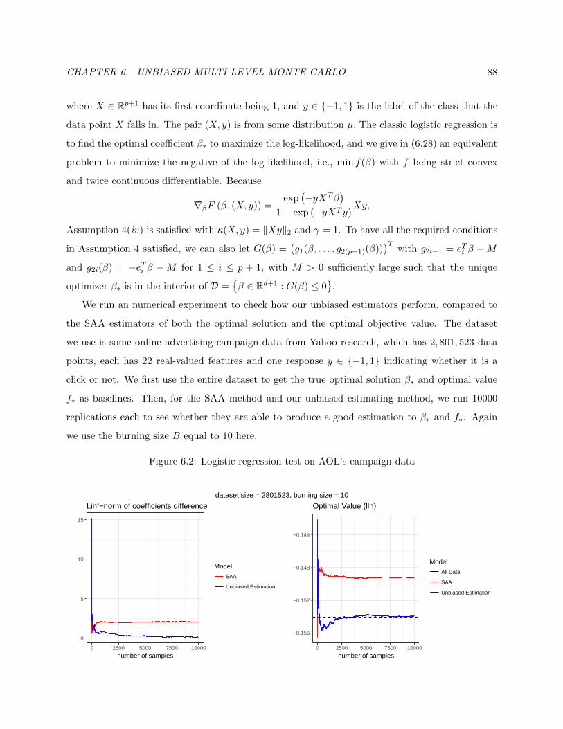
CHAPTER 6. UNBIASED MULTI-LEVEL MONTE CARLO 88
where X ∈ Rp+1 has its first coordinate being 1, and y ∈ −1, 1 is the label of the class that the
data point X falls in. The pair (X, y) is from some distribution µ. The classic logistic regression is
to find the optimal coefficient β∗ to maximize the log-likelihood, and we give in (6.28) an equivalent
problem to minimize the negative of the log-likelihood, i.e., min f(β) with f being strict convex
and twice continuous differentiable. Because
∇βF (β, (X, y)) =exp
(−yXTβ
)1 + exp (−yXT y)
Xy,
Assumption 4(iv) is satisfied with κ(X, y) = ‖Xy‖2 and γ = 1. To have all the required conditions
in Assumption 4 satisfied, we can also let G(β) =(g1(β, . . . , g2(p+1)(β))
)Twith g2i−1 = eTi β −M
and g2i(β) = −eTi β −M for 1 ≤ i ≤ p + 1, with M > 0 sufficiently large such that the unique
optimizer β∗ is in the interior of D =β ∈ Rd+1 : G(β) ≤ 0
.
We run an numerical experiment to check how our unbiased estimators perform, compared to
the SAA estimators of both the optimal solution and the optimal objective value. The dataset
we use is some online advertising campaign data from Yahoo research, which has 2, 801, 523 data
points, each has 22 real-valued features and one response y ∈ −1, 1 indicating whether it is a
click or not. We first use the entire dataset to get the true optimal solution β∗ and optimal value
f∗ as baselines. Then, for the SAA method and our unbiased estimating method, we run 10000
replications each to see whether they are able to produce a good estimation to β∗ and f∗. Again
we use the burning size B equal to 10 here.
Figure 6.2: Logistic regression test on AOL’s campaign data
0
5
10
15
0 2500 5000 7500 10000
number of samples
Model
SAA
Unbiased Estimation
Linf−norm of coefficients difference
−0.156
−0.152
−0.148
−0.144
0 2500 5000 7500 10000
number of samples
Model
All Data
SAA
Unbiased Estimation
Optimal Value (llh)dataset size = 2801523, burning size = 10

CHAPTER 6. UNBIASED MULTI-LEVEL MONTE CARLO 89
In Figure 6.2, the left plot shows how SAA estimator (in red) and the unbiased estimator (in
blue) approach the true optimal solution β∗ as we increase the size of replications, and similarly
the right plot shows the performance of both estimators for the log-likelihood (i.e., negative of the
optimal value f∗), and the baseline level of log-likelihood is represented by the black dashed line.
In both cases, our unbiased estimators beat the SAA estimators in terms of unbiasedness.
6.3 Quantile estimation
Suppose (Xk : k ≥ 1) are iid with cumulative distribution function F (x) = µ((−∞, x]) = P (X ≤ x)
for x ∈ R. We define xp = xp (µ) = infx ≥ 0 : F (x) ≥ p to be the p-quantile of distribution µ
for any given 0 < p < 1. If F (·) is continuous we have that
F (xp) = p.
Connecting to the general framework from Section 5.1, here we have θ (µ) := xp (µ).
We first impose some assumptions.
Assumption 5. Distributional quantile assumptions:
(i) F is at least twice differentiable in some neighborhood of xp,
(ii) F ′′(x) is bounded in the neighborhood,
(iii) F ′(xp) = f(xp) > 0,
(iv) E[X2]<∞.
Note that Assumptions 5(i), 5(ii) and 5(iii) ensure xp is the unique p-quantile of distribution
µ. By Bahadur representation of sample quantiles in [Bahadur, 1966], we have
Yn = xp +np− Znnfµ (xp)
+Rn, (6.29)
where
Yn = (1− wn)X[np] + wnX[np]+1, wn = np− [np] ∈ [0, 1), (6.30)
i.e., the sample p−quantile of sample (X1, . . . , Xn), Zn =∑n
i=1 I (Xi ≤ xp) and Rn =
O(n−3/4 log n
)as n→∞ almost surely.
Lemma 8. If Assumption 5 is in force, supn≥1/pE[Y 2n
]<∞.

CHAPTER 6. UNBIASED MULTI-LEVEL MONTE CARLO 90
Proof. Just follow Bahadur’s proof. Let
Gn(x, ω) = (Fn(x, ω)− Fn(xp, ω))− (F (x)− F (xp)) ,
and let In be an open interval (xp−an, xp+an) with the constant an ∼ log n/√n as n→∞. Define
Hn(ω) = sup |Gn(x, ω)| : x ∈ In .
By Lemma 1 in [Bahadur, 1966], Hn(ω) ≤ Kn(ω) + βn with βn = O(n−3/4 log n
),∑
n P (Kn ≥ γn) <∞ and γn = cn−3/4 log n. By Lemma 2 in [Bahadur, 1966] we have Yn ∈ In for
sufficiently large n w.p.1. Let n∗ = supnKn ≥ γn or Yn /∈ In <∞, then for all n ≥ 1/p
E[Y 2n
]= E
[Y 2n I (n ≤ n∗)
]+ E
[Y 2n I (n > n∗)
],
where
E[Y 2n I (n ≤ n∗)
]≤ E
[n∑i=1
X2i I (n ≤ n∗)
]≤ n∗E
[X2]<∞,
and
E[Y 2n I (n > n∗)
]= E
[(xp +
np− Znnf (xp)
+Rn
)2
I (n > n∗)
]≤ 3x2
p +3pq
nf (xp)2 + 3E
[R2nI (n > n∗)
]≤ 3x2
p +3pq
nf (xp)2 + 3E
[H2nI (n > n∗)
]≤ 3x2
p +3pq
nf (xp)2 + 6γ2
n + 6β2n <∞.
Combining these two parts together we can conclude supnE[Y 2n
]<∞.
We let Y2n+1 denote the sample p−quantile of (X1, · · · , X2n+1), let Y O2n denote the sample
p−quantile of the odd indexed sub-sample(XO
1 , · · · , XO2n)
and let Y E2n denote the sample p−quantile
of the even indexed sub-sample(XE
1 , · · · , XE2n). Then, define
∆n = Y2n+1 − 1
2
(Y O
2n + Y E2n). (6.31)
Let nb = minn ∈ N : n ≥ 1/p. We let the geometrically distributed random variable N to take
values on nb, nb + 1, . . . with p (n) = P (N = n) > 0 for all n ≥ nb. Define the estimator to be
Z =∆N
p (N)+ Y2nb . (6.32)
CHAPTER 6. UNBIASED MULTI-LEVEL MONTE CARLO 91
Theorem 5. If Assumption 5 are in force, then E [Z] = xp, V ar(Z) < ∞ and the computation
complexity required to produce Z is bounded in expectation.
Proof. We first show the unbiasedness of Z. Uniform integrability of Y2n : n ≥ nb is established
in Lemma 8 with Assumption 5(iv) holds true, so we have
E [Z] =∞∑
n=n0
E [∆n] + E [Y2n0 ] = limn→∞
E [Y2n ] = E[
limn→∞
Y2n
]= xp.
We next show V ar(Z) <∞. With (6.29) we have
∆n =
(xp +
2n+1p− Z2n+1
2n+1f (xp)+R2n+1
)− 1
2
[(xp +
2np− ZO2n2nf (xp)
+RO2n
)+
(xp +
2np− ZE2n2nf (xp)
+RE2n
)]= R2n+1 − 1
2
(RO2n +RE2n
)= O
(n · 2−3n/4
)w.p.1,
thus ∆2n = O
(n2 · 2−3n/2
). Again by Lemma 8 and (6.29), we have supnE
[R2n
]<∞, hence ∆n :
n ≥ n0 is uniformly integrable and E[∆2n
]= O
(n2 · 2−3n/2
). If we choose p(n) = r(1 − r)n−nb
with r < 1− 12√
2for n ≥ nb, then
E
[∣∣∣∣ ∆N
p(N)
∣∣∣∣2]
=∞∑
n=nb
E[∆2n]
p(n)<∞,
thus V ar(Z) <∞.
Finally we show the computation cost of generating ∆n is finite in expectation. Each replication
of Z involves simulating 2N+1 independent copies of X. If we adopt the selection method based on
random partition introduced in [Blum et al., 1973], then it will cost us O(2N+1
)time to identify the
sample p−quantiles Y2N+1 , Y O2N
, and Y E2N
. Therefore by letting N be an independent geometrically
distributed random variable with success parameter r ∈(1/2, 1− 2−3/2
), Z is an unbiased estimator
of the true unique p-quantile xp and it has finite work-normalized variance.

92
Part III
Bibliography

BIBLIOGRAPHY 93
Bibliography
[Agarwal and Gobet, 2017] A. Agarwal and E. Gobet. Finite variance unbiased estimation of
stochastic differential equations. In 2017 Winter Simulation Conference (WSC), pages 1950–
1961, Dec 2017.
[Asmussen and Glynn, 2007] S. Asmussen and P.W. Glynn. Stochastic Simulation: Algorithms and
Analysis. Springer-Verlag New York, 2007.
[Asmussen et al., 1992] S. Asmussen, P.W. Glynn, and H. Thorisson. Stationarity detection in the
initial transient problem. ACM Transactions on Modeling and Computer Simulation (TOMACS),
2(2):130–157, 1992.
[Asmussen, 2003] S. Asmussen. Applied Probability and Queues. Springer, 2 edition, 2003.
[Bahadur, 1966] R.R. Bahadur. A note on quantiles in large samples. The Annals of Mathematical
Statistics, 37(3):577–580, 06 1966.
[Bahr, 1965] B.V. Bahr. On the convergence of moments in the Central Limit Theorem. The
Annals of Mathematical Statistics, 36(3):808–818, 1965.
[Blanchet and Chen, 2015] J. Blanchet and X. Chen. Steady-state simulation of reflected Brownian
motion and related stochastic networks. Annals of Applied Probability, 25(6):3209–3250, 2015.
[Blanchet and Dong, 2013] J. Blanchet and J. Dong. Perfect sampling for infinite server and loss
systems. Advances in Applied Probability, 47, 12 2013. Forthcoming in Advances in Applied
Probability.

BIBLIOGRAPHY 94
[Blanchet and Glynn, 2015] J. Blanchet and P.W. Glynn. Unbiased Monte Carlo for optimization
and functions of expectations via multi-level randomization. In Proceedings of the 2015 Winter
Simulation Conference, WSC ’15, pages 3656–3667. IEEE Press, 2015.
[Blanchet and Sigman, 2011] J. Blanchet and K. Sigman. On exact sampling of stochastic perpe-
tuities. Journal of Applied Probability, 48(A):165–182, 2011.
[Blanchet and Wallwater, 2015] J. Blanchet and A. Wallwater. Exact sampling fot the station-
ary and time-reversed queues. ACM Transactions on Modeling and Computer Simulation
(TOMACS), 25(4):26:1–26:27, 2015.
[Blum et al., 1973] M. Blum, R.W. Floyd, V. Pratt, R.L. Rivest, and R.E. Tarjan. Time bounds
for selection. Journal of Computer and System Sciences, 7(4):448 – 461, 1973.
[Chen and Yao, 2013] H. Chen and D.D. Yao. Fundamentals of queueing networks: Performance,
asymptotics, and optimization, volume 46. Springer Science & Business Media, 2013.
[Connor and Kendall, 2007] S.B. Connor and W.S. Kendall. Perfect simulation for a class of posi-
tive recurrent Markov chains. The Annals of Applied Probability, 17(3):781–808, 06 2007.
[Connor and Kendall, 2015] S.B. Connor and W.S. Kendall. Perfect simulation of M/G/c queues.
Advances in Applied Probability, 47(4):1039–1063, 12 2015.
[Corcoran and Tweedie, 2001] J.N. Corcoran and R.L. Tweedie. Perfect sampling of ergodic Harris
chains. The Annals of Applied Probability, 11(2):438–451, 05 2001.
[Crisan et al., 2018] D. Crisan, P. Del Moral, J. Houssineau, and A. Jasra. Unbiased multi-index
Monte Carlo. Stochastic Analysis and Applications, 36(2):257–273, 2018.
[Dai, 2011] H. Dai. Exact Monte Carlo simulation for Fork-Join networks. Advances in Applied
Probability, 43(2):484–503, 03 2011.
[Del Moral, 2004] P. Del Moral. Feynman-Kac Formulae Genealogical and Interacting Particle
Systems with Applications. Springer-Verlag, 2004.
[Dereich and Mueller-Gronbach, 2017] S. Dereich and T. Mueller-Gronbach. General multilevel
adaptions for stochastic approximation algorithms. arXiv:1506.05482, 2017.

BIBLIOGRAPHY 95
[Ensor and Glynn, 2000] K. Ensor and P.W. Glynn. Simulating the maximum of a random walk.
Journal of Statistical Planning and Inference, 85:127–135, 2000.
[Flatto and Hahn, 1984] L. Flatto and S. Hahn. Two parallel queues created by arrivals with two
demands. SIAM Journal on Applied Mathematics, 44(5):1041–1053, 1984.
[Foss and Chernova, 2001] S.G. Foss and N.I. Chernova. On optimality of the FCFS discipline
in multiserver queueing systems and networks. Siberian Mathematical Journal, 42(2):372–385,
2001.
[Foss and Konstantopoulos, 2006] S.G. Foss and T. Konstantopoulos. Lyapunov function methods.
Lecture Notes, 2006.
[Foss and Tweedie, 1998] R.L. Foss and R.L. Tweedie. Perfect simulation and backward coupling.
Stochastic Models, 14:187–203, 1998.
[Foss, 1980] S.G. Foss. Approximation of multichannel service systems. Sibirsk. Mat. Zh.,
21(6):132–140, 1980.
[Gao and Zhao, 2011] F. Gao and X. Zhao. Delta method in large deviations and moderate devi-
ations for estimators. The Annals of Statistics, 39(2):1211–1240, 2011.
[Garmarnik and Goldberg, 2013] D. Garmarnik and D. Goldberg. Steady-state GI/GI/n queue in
the Halfin-Whitt regime. Annals of Applied Probability, 23:2382–2419, 2013.
[Giles and Szpruch, 2014] M.B. Giles and L. Szpruch. Antithetic multilevel Monte Carlo estimation
for multi-dimensional SDEs without Levy area simulation. The Annals of Applied Probability,
24(4):1585–1620, 08 2014.
[Giles, 2008] M.B. Giles. Multilevel Monte Carlo path simulation. Operations Research, 56(3):607–
617, 2008.
[Hillier and Lo, 1971] F.S. Hillier and F.D. Lo. Tables for multiple-server queueing systems involv-
ing Erlang distributions. Technical Report 31, Department of Operations Research, Stanford
University, 1971.
[Kelly, 1979] F.P. Kelly. Reversibility and stochastic networks, volume 40. Wiley, 1979.
BIBLIOGRAPHY 96
[Kendall and Møller, 2000] W.S. Kendall and J. Møller. Perfect simulation using dominating pro-
cesses on ordered spaces, with application to locally stable point processes. Advances in Applied
Probability, pages 844–865, 2000.
[Kendall, 1998] W.S. Kendall. Perfect simulation for the area-interaction point process. In Proba-
bility towards 2000, pages 218–234. Springer, 1998.
[Kendall, 2004] W.S. Kendall. Geometric ergodicity and perfect simulation. Electron. Comm.
Probab., 9:140–151, 2004.
[Khodadadian et al., 2018] A. Khodadadian, L. Taghizadeh, and C. Heitzinger. Optimal multi-
level randomized quasi-Monte-Carlo method for the stochastic drift–diffusion-Poisson system.
Computer Methods in Applied Mechanics and Engineering, 329:480 – 497, 2018.
[Liu et al., 1995] Z. Liu, P. Nain, and D. Towsley. Sample path methods in the control of queues.
Queueing Systems, 21(1-2):293–335, 1995.
[Liu, 2008] J.S. Liu. Monte Carlo Strategies in Scientific Computing. Springer, 2008.
[McLeish, 2012] D. McLeish. A general method for debiasing a Monte Carlo estimator. Monte
Carlo Methods and Applications, 17(4):301–315, 2012.
[Propp and Wilson, 1996] J. Propp and D. Wilson. Exact sampling with coupled Markov chains
and applications to statistical mechanics. Random Structures and Algorithms, 9:223–252, 1996.
[Rhee and Glynn, 2015] C. Rhee and P.W. Glynn. Unbiased estimation with square root conver-
gence for SDE models. Operations Research, 63(5):1026–1043, 2015.
[Rubinstein and Kroese, 2011] R.Y. Rubinstein and D.P. Kroese. Simulation and the Monte Carlo
method, volume 707. John Wiley & Sons, 2011.
[Shapiro et al., 2009] A. Shapiro, D. Dentcheva, and A. RuszczyAski. Lectures on Stochastic Pro-
gramming. Society for Industrial and Applied Mathematics, 2009.
[Sigman, 1988] K. Sigman. Regeneration in tandem queues with multiserver stations. Journal of
Applied Probability, 25(2):291—403, 1988.

BIBLIOGRAPHY 97
[Sigman, 1995] K. Sigman. Stationary Marked Point Processes. An Intuitive Approach. Chapman
& Hall, New York, 1995.
[Sigman, 2011] K. Sigman. Exact simulation of the stationary distribution of the FIFO M/G/c
queue. Journal of Applied Probability, 48A:209–216, 2011.
[Sigman, 2012] K. Sigman. Exact sampling of the stationary distribution of the FIFO M/G/c
queue: the general case for ρ < c. Queueing Systems, 70:37–43, 2012.
[Vihola, 2018] M. Vihola. Unbiased estimators and multilevel Monte Carlo. Operations Research,
66(2):448–462, 2018.
[Wachsmuth, 2013] G. Wachsmuth. On LICQ and the uniqueness of Lagrange multipliers. Opera-
tions Research Letters, 41(1):78–80, 2013.
[Wolff, 1977] R.W. Wolff. An upper bound for multi-channel queues. Journal of Applied Probability,
14:884–888, 1977.
[Wolff, 1987] R.W. Wolff. Upper bounds on work in system for multichannel queues. Journal of
Applied Probability, 24(2):547–551, 1987.
[Wolff, 1989] R.W. Wolff. Stochastic Modeling and the Theory of Queues. Prentice Hall, New
Jersey, 1989.
[Xu, 2010] H. Xu. Uniform exponential convergence of sample average random functions under
general sampling with applications in stochastic programming. Journal of Mathematical Analysis
and Applications, 368, 2010.

98
Part IV
Appendices

APPENDIX A. APPENDIX TO CHAPTER 3 99
Appendix A
Appendix to Chapter 3
A.1 The iid property of the coupled service times and indepen-
dence of the arrival process
In order to explain why the Vn form an iid sequence, independent of the sequence T 0 = T 0n : n ∈
Z\0, it is useful to keep in mind the diagram depicted in Figure A.1, which illustrates a case
involving two servers, c = 2.
The assignment of the service times, as we shall explain, can be thought of as a procedure
similar to a Tetris game. Arrival times are depicted by dotted horizontal lines which go from left
to right, starting at the left most vertical line, which is labeled “Arrivals”. Think of the time line
going, vertically, from the bottom of the graph (past) to the top of the graph (future).
In the right-most column in Figure A.1, we indicate the queue length, right at the time of a
depicted arrival (and thus, including the arrival itself). So, for example, the first arrival depicted
in Figure A.1 observes one customer waiting and thus, including the arrival himself, there are two
customers waiting in queue.
The Tetris configuration observed by an arrival at time T is comprised of two parts: (i) the
receding horizon, which corresponds to the remaining incomplete blocks, and (ii) the landscape,
comprised of the configuration of complete blocks. So, for example, the first arrival in Figure A.1
observes a receding horizon corresponding to the two white remaining blocks, which start from the
dotted line at the bottom. The landscape can be parameterized by a sequence of block sizes, and
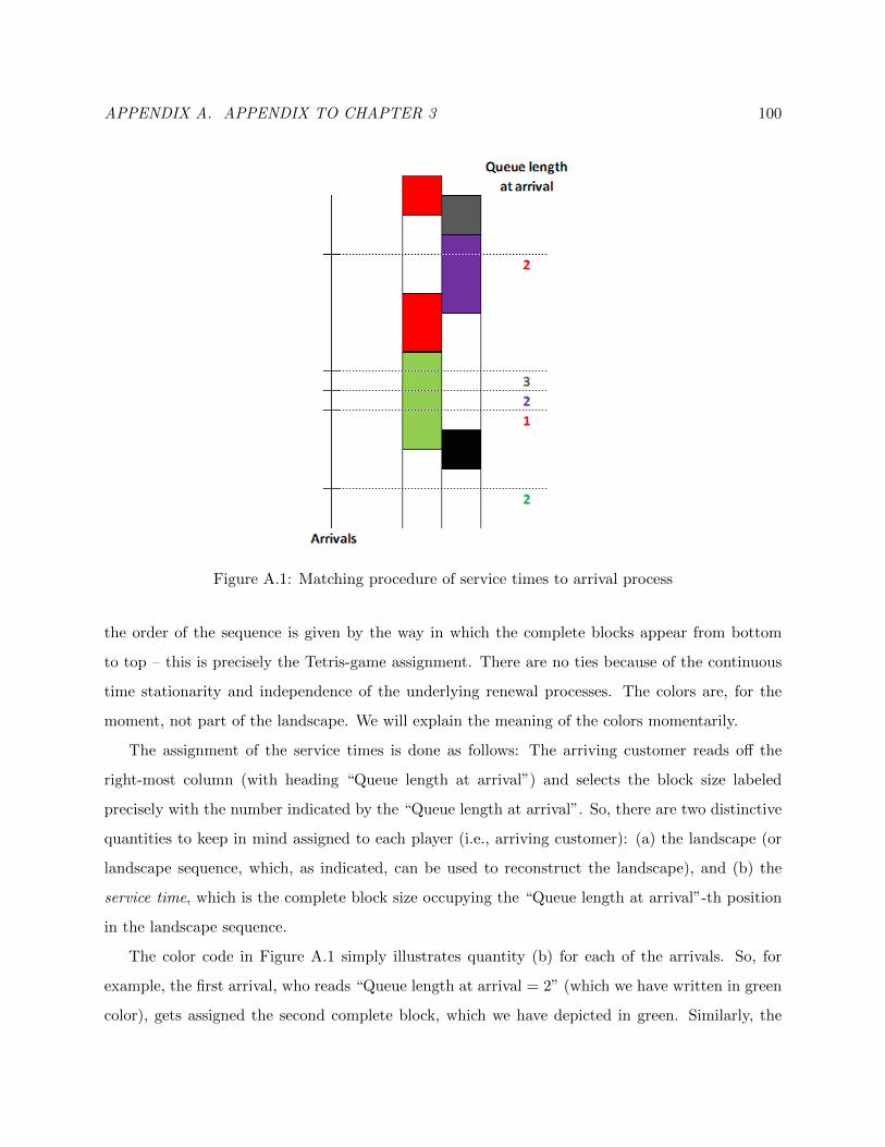
APPENDIX A. APPENDIX TO CHAPTER 3 100
Figure A.1: Matching procedure of service times to arrival process
the order of the sequence is given by the way in which the complete blocks appear from bottom
to top – this is precisely the Tetris-game assignment. There are no ties because of the continuous
time stationarity and independence of the underlying renewal processes. The colors are, for the
moment, not part of the landscape. We will explain the meaning of the colors momentarily.
The assignment of the service times is done as follows: The arriving customer reads off the
right-most column (with heading “Queue length at arrival”) and selects the block size labeled
precisely with the number indicated by the “Queue length at arrival”. So, there are two distinctive
quantities to keep in mind assigned to each player (i.e., arriving customer): (a) the landscape (or
landscape sequence, which, as indicated, can be used to reconstruct the landscape), and (b) the
service time, which is the complete block size occupying the “Queue length at arrival”-th position
in the landscape sequence.
The color code in Figure A.1 simply illustrates quantity (b) for each of the arrivals. So, for
example, the first arrival, who reads “Queue length at arrival = 2” (which we have written in green
color), gets assigned the second complete block, which we have depicted in green. Similarly, the

APPENDIX A. APPENDIX TO CHAPTER 3 101
second arrival depicted reads off the number “1” (written in red) and gets assigned the first red
block depicted (from bottom to top). The very first complete block (from bottom to top), which is
depicted in black, corresponds to the service time assigned to the customer ahead of the customer
who collected the green block. The number “1” (in red) is obtained by observing that the customer
with the initial black block has departed.
Now we argue the following properties:
(1) The service times are iid copies of V .
(2) The service times are independent of T 0.
About property (1): The player arriving at time T reads a number, corresponding to the queue
length, which is obtained by the past filtration FT generated by ∪k∈Z\0,0≤i≤cT ik : T ik ≤ T.Conditional on the receding horizon (i.e., remaining incomplete block sizes), RT , the past filtration
is independent of the landscape. This is simply the Markov property applied to the forward residual
lifetime process of each of the c renewal processes represented by the c middle columns. Moreover,
conditional on RT , each landscape forms a sequence of iid copies of V because of the structure of
the underlying c renewal processes corresponding to the middle columns. So, let Q (T ) denote the
queue length at time T (including the arrival at time T ), which is a function of the past filtration,
and let LT (k) : k ≥ 1 be the landscape sequence observed at time T , so that LT (Q (T )) is
the service time of the customer who arrives at time T . We then have that for any positive and
bounded continuous function f (·),
E[f (LT (Q (T ))) |RT ] = E[f (LT (1)) |RT ] = E[f (V )],
precisely because, conditional on RT , Q (T ) (being FT measurable) is independent of
LT (k) : k ≥ 1.To verify the iid property, let f1, f2 be non-negative and bounded continuous functions. Assume
that T1 < T2 are arrival times in T 0 (not necessarily consecutive). Then,
E[f1 (LT1 (Q (T1))) f2 (LT2 (Q (T2)))]
= E[E[f1 (LT1 (Q (T1))) f2(LT2 (Q (T2)))|FT2 ,RT2 ]]
= E[f1 (LT1 (Q (T1)))E[f2(LT2 (Q (T2)))|FT2 ,RT2 ]]
= E[f1(LT1 (Q (T1)))]E[f2(V )] = E[f1(V )]E[f2(V )].
APPENDIX A. APPENDIX TO CHAPTER 3 102
The same argument extends to any subset of arrival times, and thus the iid property follows.
About property (2): Note that in the calculations involving property (1), the actual values of
the arrival times T , T1 and T2 are irrelevant. The iid property of the service times is established
path-by-path conditional on the observed realization T 0. Thus, the independence of the arrival
process and service times follows immediately.
A.2 Proof of technical lemmas of monotonicity
Proof of Lemma 1. Both facts are standard; the first one can be easily shown using induc-
tion. Specifically, we first notice that Wk(T0k ;w+) = w+ > w− = Wk(T
0n ;w−). Suppose that
Wk(T0n ;w+) ≥Wk(T
0n ;w−) for some n ≥ k, then
Wk(T0,+n ;w+) = S
((Wk(T
0n ;w+) + Vne1 −An1
)+)≥ S
((Wk(T
0n ;w−) + Vne1 −An1
)+)= Wk(T
0,+n ;w−).
For inequality (3.9), we note that Wk
(T 0k′ ; 0
)≥ Wk′
(T 0k′ ; 0
)= 0, and therefore, due to (3.8), we
have that
Wk
(T 0n ; 0)
= Wk′(T 0n ;Wk (Tk′ ; 0)
)≥Wk′
(T 0n ; 0).
Proof of Lemma 2. This fact follows immediately by induction from Eqs. (3.4) and (3.7) using the
fact that Ξn ≥ 0.
Proof of Lemma 3. We first prove the inequality Qu(t − u; z+) ≤ Qv(t). Note that U i (u) > 0 for
all u (the forward residual life time process is right continuous), so the initial condition r indicates
that all the servers are busy (operating) and the initial q ≥ 0 customers will leave the queue (i.e.,
enter service) at the same time as those in the vacation system under the evolution of Zu (·; z+).
Now, let us write N = infn : T 0n ≥ u (in words, the next arriving customer at or after u arrives
at time T 0N ). It is easy to see that S
(U(T 0N
))≥ Ru(T 0
N − u; z+); to wit, if T 0N occurs before
any of the servers becomes idle, then we have equality, and if T 0N occurs after, say, l ≥ 1 servers

APPENDIX A. APPENDIX TO CHAPTER 3 103
become idle, then Ru(T 0N − u; z+) will have l zeroes and the bottom c− l entries will coincide with
those of S(U(T 0N
)), which has strictly positive entries. So, if wN is the Kiefer-Wolfowitz vector
observed by the customer arriving at T 0N (induced by Qu(· − u; z+)), then we have Wv (N) ≥ wN .
By monotonicity of the Kiefer-Wolfowitz vector in the initial condition and because of Lemma 2,
we have
Wv (k) ≥WN
(T 0k ;Wv (N)
)≥WN
(T 0k ;wN
),
for all k ≥ N , and hence, T 0k +D0
k ≥ T 0k +W
(1)N
(T 0k ;wN
). Therefore, the departure time from the
queue (i.e., initiation of service) of the customer arriving at T 0k in the vacation system occurs no
earlier than the departure time from the queue of the customer arriving at time T 0k in the GI/GI/c
queue. Consequently, we conclude that the set of customers waiting in the queue in the GI/GI/c
system at time t is a subset of the set of customers waiting in the queue in the vacation system at
the same time. Similarly, we consider Qu(t − u; z−) ≤ Qu(t − u; z+), which is easier to establish,
since, for k ≥ N (with the earlier definition of T 0N and wN ),
WN
(T 0k ;wN
)≥WN
(T 0k ; 0),
So the set of customers waiting in the queue in the lower bound GI/GI/c system at time t is a
subset of the set of customers waiting in the queue in the upper bound GI/GI/c system at the
same time.

APPENDIX B. APPENDIX TO CHAPTER 4 104
Appendix B
Appendix to Chapter 4
B.1 Detailed algorithm steps in Section 4.2.1
To simulate the process (S(r)n , W 0
−n) : 0 ≤ n ≤ N with the stopping time N defined in (4.17) as
N = inf
n ≥ 0 : W 0
−n = maxk≥n
S(r)k − S(r)
n = 0
,
we must sample the running time maxima (entry by entry) of the c-dimensional random walk
S(r)n =
n∑i=1
∆−i =n∑i=1
(V−iu−i −A−i1) n ≥ 0.
We will find a sequence of random times Nn : n ≥ 1 such that maxn≤k≤Nn S(r)k ≥ maxk≥Nn S
(r)k .
Hence, we will be able to find the running time maxima by only sampling the random walk on a
finite time interval, i.e., Nn is such that
maxk≥n
S(r)k = max
n≤k≤NnS
(r)k .
To achieve this, we first decompose the random walk into two random walks, and then construct a
sequence of “milestone” events for each of these two random walks to detect Nn. We will elaborate
the detailed implementations in the following context.
Because of the stability condition ρ = λ/(cµ) < 1, we can find some value a ∈ (1/µ, c/λ). For

APPENDIX B. APPENDIX TO CHAPTER 4 105
any n ≥ 0, define
X−n =n∑j=1
(V−j − a) u−j , (B.1)
Y−n =
n∑j=1
(au−j −A−j1) , (B.2)
hence S(r)n =
∑nj=1 ∆−j = X−n + Y−n and maxk≥n S
(r)k = maxk≥n(X−n + Y−n).
For all n ≥ 0, let
NXn = infn′ ≥ n : max
k≥n′X−k ≤ X−n, (B.3)
NYn = infn′ ≥ n : max
k≥n′Y−k ≤ Y−n, (B.4)
Nn = maxNXn , N
Yn . (B.5)
Then, by the definitions above,
maxk≥Nn
S(r)k ≤ max
k≥NnX−k + max
k≥NnY−k ≤ X−n + Y−n = S(r)
n .
Therefore, to get the running-time maximum maxk≥n S(r)k for each n ≥ 0, we only need to sample
the random walk from step n to Nn, because
maxk≥n
S(r)k = max max
n≤k≤NnS
(r)k , max
n≥NnS
(r)k = max
n≤k≤NnS
(r)k .
Next, we describe how to sample Nn along with the multi-dimensional random walks X−n :
n ≥ 0 and Y−n : n ≥ 0.
B.1.1 Simulation algorithm for the process Y−n : n ≥ 0
We first consider simulating the c-dimensional random walk Y−n : n ≥ 0 with Y0 = 0. For each
j ≥ 1, E [au−j −A−j1] < 0, we can simulate the running time maximum maxk≥n Y−k jointly with
the path Y−k : 0 ≤ k ≤ n via the exponential change of measure method developed in [Blanchet
and Chen, 2015], with the following assumptions.
Assumption 6. There exits θ > 0, θ ∈ Rc such that
E[exp
(θT (au−j −A−j1)
)]<∞.

APPENDIX B. APPENDIX TO CHAPTER 4 106
Assumption 7. Suppose that in every dimension i = 1, . . . , c, there exists θ∗ ∈ (0,∞) such that
φi(θ∗) := logE [exp (θ∗ (aI(U−j = i)−A−j))] = 0.
Because for each j ≥ 1, aI(U−j = i)−A−j are marginally identically distributed across i, so θ∗
would work for all i = 1, . . . , c.
Remark 4. Assumption 7 is known as Cramer’s condition in the large deviations literature and
it is a strengthening of Assumption 6. We shall explain briefly at the end of this section that it is
possible to relax this assumption to Assumption 6 by modifying the algorithm a bit without affecting
the exactness/computational effort of the algorithm. For the moment we continue to describe the
main algorithmic idea under Assumption 7.
For any s ∈ Rc and b ∈ Rc+ define
Tb = infn ≥ 0 : Y−n(i) > b(i) for some i ∈ 1, . . . , c, (B.6)
T−b = infn ≥ 0 : Y−n(i) < −b(i) for all i = 1, . . . , c, (B.7)
Ps(·) = P (·|Y0 = s). (B.8)
We will use these definitions in Algorithm LTGM given in Section B.1.1.1.
We next construct a sequence of upward and downward “milestone” events for this multi-
dimensional random walk. Let
m = dlog(c)/θ∗e. (B.9)
Define D0 = 0 and Γ0 =∞. For k ≥ 1, let
Dk = infn ≥ Dk−1 ∨ Γk−1I (Γk−1 <∞) : Y−n(i) < Y−Dk−1(i)−m for all i, (B.10)
Γk = infn ≥ Dk : Y−n(i) > Y−Dk(i) +m for some i, (B.11)
where m is defined in (B.9). Note that by convention, ΓkI (Γk <∞) = 0 if Γk =∞ for any k ≥ 0.
We let B ∈ Rc, initially set as (∞, . . . ,∞)T ∈ Rc, to be the running time upper bound of process
Y−n : n ≥ 0. Let m = m1. From the construction of “milestone” events in (B.10) and (B.11),
we know that if Γk =∞ for some k ≥ 1, the process will never cross over the level Y−Dk + m after
Dk coordinate-wise, i.e., for i = 1, . . . , c,
Y−n(i) ≤ Y−Dk(i) +m, ∀n ≥ Dk.
Hence, in this case we update the upper bound vector B = Y−Dk + m.

APPENDIX B. APPENDIX TO CHAPTER 4 107
B.1.1.1 Global maximum simulation
Define
Λ = infDk : Γk =∞, k ≥ 1. (B.12)
By the construction of “milestone” events, for all n ≥ Λ
Y−n ≤ Y−Λ + m < 0 = Y0.
Hence, we can evaluate the global maximum level of the process Y−n : n ≥ 0 to be
M0 := maxk≥0
Y−k = max0≤k≤Λ
Y−k, (B.13)
and we give the detailed sampling procedure in the following algorithm. The algorithm has elements,
such as sampling from P0(Tm <∞), which will be explained in the sequel.
Algorithm LTGM: Simulate global maximum of c-dimensional process Y−n : n ≥ 0 jointly with
the sub-path and the subsequence of “milestone” events.
Input: a ∈ (1/µ, c/λ) satisfies Assumption 7, m as in (B.9).
1. (Initialization) Set n = 0, Y0 = 0, D = [0], Γ = [∞], L = 0 and B =∞1.
2. Generate U ∼ Unif1, . . . , c and let u = (I(U = 1), . . . , I(U = c))T . Independently sample
A ∼ G. Set n = n+ 1, Y−n = Y−(n−1) + au−A1, U−n = U and A−n = A.
3. If there is some 1 ≤ i ≤ c such that Y−n(i) ≥ L(i) − m, then go to Step 2; otherwise set
D = [D, n] and L = Y−n.
4. Independently sample J ∼ Ber (P0 (Tm <∞)).
5. If J = 1, simulate a new conditional path (Y−k, U−k, A−k
): 1 ≤ k ≤ Tm with Y0 = 0,
following the conditional distribution of Y−k : 0 ≤ k ≤ Tm given Tm < ∞. Set Y−(n+k) =
Y−n + Y−k, U−(n+k) = U−k, A−(n+k) = A−k for 1 ≤ k ≤ Tm. Set n = n+ Tm, Γ = [Γ, n]. Go
to Step 2.
6. If J = 0, set Λ = n, Γ = [Γ,∞] and B = L+ m.

APPENDIX B. APPENDIX TO CHAPTER 4 108
7. Output (Y−k, U−k, T−k) : 1 ≤ k ≤ Λ, D, Γ and global maximum M0 = max0≤k≤Λ Y−k.
Now we explain how to execute Steps 4 and 5 in the previous algorithm. The procedure is
similar to the multi-dimensional procedure given in [Blanchet and Chen, 2015], so we describe it
briefly here. As P0(·) denotes the canonical probability, we let P ∗0 (·) = P0(·|Tm < ∞). Our goal
is to simulate from the conditional law of Y−k : 0 ≤ k ≤ Tm given that Tm < ∞ and Y0 = 0,
i.e., to simulate from P ∗0 . We will use acceptance/rejection by letting P ′0(·) denote the proposal
distribution. A typical element ω′ sampled under P ′0(·) is of the form ω′ = ((Y−k : k ≥ 0), index),
where index ∈ 1, · · · , c and it indicates the direction we pick to do exponential tilting. Given
the value of index, the process (Y−k : k ≥ 0) remains a random walk. We now describe P ′0 by
explaining how to sample ω′. First,
P ′0 (index = i) :=1
c. (B.14)
Then, conditioning on index = i, for every set Ω ∈ σ (Y−k : 0 ≤ k ≤ n),
P ′0 (Ω|index = i) = E0 (exp (θ∗Y−n(i)) IΩ) . (B.15)
To obtain the induced distribution for U and A, we study the moment generating function
induced by definition (B.15). Given η ∈ Rc in a neighborhood of the origin,
E0 exp(ηT (au−A1) + θ∗eTi (au−A1)
)E0 exp
(θ∗eTi (au−A1)
) =E0 exp
((η + θ∗ei)
Tau)
E0 exp(θ∗eTi au
) · E0 exp(−(η + θ∗ei)
TA1)
E0 exp(−θ∗eTi A1
) .
The previous expression indicates that under P ′0(·), A and U are independent. Moreover, we have
E0
[exp
(θ∗eTi au
)]=
exp(θ∗a) + c− 1
c.
Therefore,
P ′0(U = j|index = i) =
exp(θ∗a)
exp(θ∗a)+c−1 if j = i
1exp(θ∗a)+c−1 if j 6= i
. (B.16)
On the other hand, conditional on index = i, the distribution of a generic interarrival time A is
obtained by exponential tilting such that
dP0(A|index = i) = dP0(A) · exp(−θ∗A)
E0 exp(−θ∗A)
= dP0(A) · exp(aθ∗) + c− 1
c exp(θ∗A), (B.17)

APPENDIX B. APPENDIX TO CHAPTER 4 109
where the second equation follows from Assumption 7.
Following Assumption 7, and because V ar(aI(U−j = i)−A−j) > 0, by convexity,
E′0 (Y−n(index)) =c∑i=1
E0 (Y−n(i) exp (θ∗Y−n(i)))P ′0 (index = i)
=1
c
c∑i=1
dφi (θ∗)
dθ> 0,
so Y−n (index) → ∞ as n → ∞ almost surely under P ′0(·), hence Tm < ∞ with probability one
under P ′0(·). Now, to verify that P0(·) is a valid proposal for acceptance/rejection method, we must
verify that dP ∗0/dP′0 is bounded by a constant, i.e.,
dP ∗0dP ′0
(Y−k : 0 ≤ k ≤ Tm)
=1
P0 (Tm <∞)× dP0
dP ′0(Y−k : 0 ≤ k ≤ Tm)
=1
P0 (Tm <∞)× 1∑c
i=1wi exp (θ∗Y−Tm(i))
≤ 1
P0 (Tm <∞)× c
exp (θ∗m)
<1
P0 (Tm <∞),
where the last inequality is guaranteed by (B.9). So, acceptance/rejection is valid.
Moreover, the overall probability of accepting the proposal is precisely P0(Tm <∞). Thus, we
not only execute Step 5, but simultaneously also Step 4. We use this acceptance/rejection method
to replace Steps 4 and 5 in Algorithm LTGM as follows:
4’ Sample(Y−k, U−k, A−k
): 0 ≤ k ≤ Tm
) with Y0 = 0 from P ′0 (·) as indicated via (B.14),
(B.16) and (B.17). Sample a Bernoulli J with success probability
c∑ci=1 exp
(θ∗Y−Tm(i)
) .5’ If J = 1, set Y−(n+k) = Y−n + Y−k, U−(n+k) = U−k, A−(n+k) = A−k for 1 ≤ k ≤ Tm. Set
n = n+ Tm and Γ = [Γ, n]. Go to Step 2.

APPENDIX B. APPENDIX TO CHAPTER 4 110
B.1.1.2 Simulate Y−n : n ≥ 0 with “milestone” events
In this section we provide an algorithm to sequentially simulate the multi-dimensional random walk
Y−n : n ≥ 0 along with its downward and upward “milestone” events as defined in (B.10) and
(B.11). We first extend Lemma 3 in [Blanchet and Sigman, 2011] to multi-dimensional version as
follows.
Lemma 9. Let 0 < a < b ≤ ∞1 (coordinate-wise) and consider any sequence of bounded positive
measurable functions fk : Rc×(k+1) → [0,∞),
E0
(fT−a(Y0, · · · , Y−T−a)|Tb =∞
)=E0
(fT−a(Y0, · · · , Y−T−a) · I(Y−j(i) ≤ b(i), 0 ≤ j < T−a, 1 ≤ i ≤ c)
)· PY−T−a
(Tb =∞)
P0 (Tb =∞).
Therefore, if P ∗∗0 (·) := P0(·|Tb =∞), then
dP ∗∗0
dP0=I (Y−j(i) ≤ b(i),∀j < T−a, 1 ≤ i ≤ c) · PY−T−a
(Tb =∞)
P0(Tb =∞)≤ 1
P0 (Tb =∞). (B.18)
Lemma 9 enables us to sample a downward patch by using the acceptance/rejection method
with the nominal distribution P0 as proposal. Suppose our current position is Y−Dj (for some j ≥ 1)
and we know that the process will never go above the upper bound B (coordinate-wise). Next we
simulate the path up to time Dj+1. If we can propose a downward patch(Y−1, · · · , Y−T−m
):=(
Y−1, · · · , Y−T−m
), under the unconditional probability given Y0 = 0 and Y−k ≤m for 1 ≤ k ≤ T−m,
then we accept it with probability P0 (Tσ =∞), where σ = B−Y−Dj−Y−T−m . A more efficient way
to sample is to sequentially generate(Y−1, · · · , Y−Λ
)with Y0 = 0 as long as m0 := max0≤k≤Λ Y−k ≤
m coordinate-wise, then concatenate the sequence to previously sampled subpath. We give the
efficient implementation procedure in the next algorithm.
Algorithm LTRW: Continue to sample the process (Y−k, U−k, A−k) : 0 ≤ k ≤ n jointly with the
partially sampled “milestone” event lists D and Γ, until some stopping criteria are met.
Input: a, m, previously sampled partial process (Y−j , U−j , A−j) : 0 ≤ j ≤ l, partial “milestone”
sequences D and Γ, and the stopping criteria H.
(Note that if there is no previous simulated random walk, we initialize l = 0, D = [0] and Γ = [∞].)

APPENDIX B. APPENDIX TO CHAPTER 4 111
1. Set n = l. If n = 0, call Algorithm LTGM to get Λ, (Y−k, U−k, A−k) : 0 ≤ k ≤ Λ, D and Γ.
Set n = Λ.
2. While the stopping criteria H are not satisfied,
(a) Call Algorithm LTGM to get Λ, (Y−j , U−j , A−j) : 0 ≤ j ≤ Λ, D, Γ and M0.
(b) If M0 ≤ m, accept the proposed sequence and concatenate it to the previous sub-path,
i.e., set Y−(n+j) = Y−n + Y−j , U−(n+j) = U−j , A−(n+j) = A−j for 1 ≤ j ≤ Λ. Update the
sequences of “milestone” events to be D = [D, n + D(2 : end)], Γ = [Γ, n + Γ(2 : end)]
and set n = n+ Λ.
3. Output (Y−k, U−k, A−k) : 0 ≤ k ≤ n with updated “milestone” event sequences D and Γ.
For n ≥ 0, define
d1(n) = infDk ≥ n : Y−Dk ≤ Y−n, (B.19)
d2(n) = infDk > d1(n) : Γk =∞, (B.20)
and d2(n) is an upper bound of NYn defined in (B.4) because
maxk≥d2(n)
Y−k ≤ Y−d2(n) + m < Y−d1(n) ≤ Y−n.
Remark 5. Although Assumption 7 is a strengthening of Assumption 6, we can accommodate our
algorithms under Assumption 6. The implementation details are the same as that mentioned in the
remark section on page 15 of [Blanchet and Chen, 2015].
B.1.2 Simulation algorithm for the process X−n : n ≥ 0
Recall from (B.1) that for n ≥ 0,
X−n(i) =
n∑j=1
(V−j − a)I(U−j = i) for i = 1, . . . , c.
Define
Nk(i) =k∑j=1
I (U−j = i) , (B.21)
Ln(i) = inf k ≥ 0 : Nk(i) = n (L0(i) = 0), (B.22)
V(i)−n = V−Ln(i), (B.23)

APPENDIX B. APPENDIX TO CHAPTER 4 112
for k ≥ 0, n ≥ 0 and i = 1, . . . , c. Nk(i) denotes the total number of customers routed to server i
among the first k arrivals counting backwards in time. Ln(i) denotes the index of the n-th customer
that gets routed to server i in the common arrival stream, counting backwards in time. V(i)−n denotes
the service time of the n-the customer that gets routed to server i, counting backwards in time.
For each i = 1, . . . , c, let X(i)−n : n ≥ 0 with X
(i)0 = 0 be an auxiliary process such that
X(i)−n :=
n∑j=1
(V
(i)−j − a
)= X−Ln(i)(i). (B.24)
For n ≥ 0 and 1 ≤ i ≤ c, define
Nn(i) = inf
n′ ≥ Nn(i) : max
k≥n′X
(i)−k ≤ X
(i)−Nn(i)
, (B.25)
hence by definition, in (B.3), we have
NXn = max
LNn(1)(1), . . . , LNn(c)(c)
. (B.26)
First we develop simulation algorithms for each of the c one-dimensional auxiliary processes
(X(i)−n : n ≥ 0) : 1 ≤ i ≤ c. Next we use the common server allocation sequence U−n : n ≥ 0
(sampled jointly with the process Y−n : n ≥ 0 in Section B.1.1) with (B.21), (B.22) and (B.23)
to find NXn via (B.26) for each n ≥ 0.
“Milestone” construction and global maximum simulation For each one-dimensional aux-
iliary process X(i)−n : n ≥ 0 with i = 1, . . . , c, we adopt the algorithm developed in [Blanchet and
Wallwater, 2015] by choosing any m′ > 0 and L′ ≥ 1 properly and define the sequences of upward
and downward “milestone” events by letting D(i)0 = 0, Γ
(i)0 =∞, and for j ≥ 1,
D(i)j = infn(i) ≥ Γ
(i)j−1I(Γ
(i)j−1 <∞) ∨D(i)
j−1 : X(i)
−n(i) < X(i)
−D(i)j−1
− L′m′, (B.27)
Γ(i)j = infn(i) ≥ D(i)
j : X(i)
−n(i) − X(i)
−D(i)j
> m′, (B.28)
with the convention that if Γ(i)j =∞, then Γ
(i)j I(Γ
(i)j <∞) = 0 for any j ≥ 0.
For each i = 1, . . . , c, define
Λ(i) = infD(i)k : Γ
(i)k =∞, k ≥ 1. (B.29)
By the “milestone” construction in (B.27) and (B.28), for all n ≥ Λ(i),
X(i)−n ≤ X
(i)
−Λ(i) +m′ < 0 = X(i)0 .

APPENDIX B. APPENDIX TO CHAPTER 4 113
Therefore we can evaluate the global maximum of the infinite-horizon process X(i)−n : n ≥ 0 in
finite steps, i.e.,
M(i)0 := max
k≥0X
(i)−k = max
0≤k≤Λ(i)X
(i)−k. (B.30)
We summarize the simulation details in the following algorithm.
Algorithm GGM: Simulate global maximum of the one-dimensional process (X(i)−n, V
(i)−n) : n ≥ 0
jointly with the sub-path and the subsequence of “milestone” events.
Input: a, m′, L′.
1. (Initialization) Set n = 0, X(i)0 = 0, D(i) = [0], Γ(i) = [∞], L(i) = 0.
2. Generate V ∼ F . Set n = n+ 1, X(i)−n = X
(i)−(n−1) + V and V
(i)−n = V .
3. If X(i)−n ≥ L(i) − L′m′, go to Step 2; otherwise set D(i) = [D(i), n] and L(i) = X
(i)−n.
4. Call Algorithm 1 on page 10 of [Blanchet and Wallwater, 2015] and obtain (J, ω).
5. If J = 1, set X(i)−(n+l) = L(i) +ω(l), S
(i)−(n+l) = X
(i)−(n+l)−X
(i)−(n+l−1) +a for l = 1, . . . , length(ω).
Set n = n+ length(ω), Γ(i) = [Γ(i), n] and go to Step 2.
6. If J = 0, set Λ(i) = n, Γ(i) = [Γ(i),∞].
7. Output (X(i)−k, V
(i)−k ) : 1 ≤ k ≤ Λ(i), D(i), Γ(i) and global maximum M
(i)0 = max0≤k≤Λ(i) X
(i)−k.
B.1.2.1 Simulate X−n : n ≥ 0 with “milestone” events
In this section, we first explain how to sample the auxiliary one-dimensional processes X(i)−n : n ≥ 0
along with the “milestone” events defined in (B.27) and (B.28). Next we will need the service
allocation information U−n : n ≥ 0, from the simulation procedure of process Y−n : n ≥ 0, to
recover the multi-dimensional process of interest X−n : n ≥ 0 via Eq. (B.24).
The following algorithm gives the the sampling procedure for each auxiliary one-dimensional
process X(i)−n : n ≥ 0 for i = 1, . . . , c. The simulation steps are the same as the procedure given
in Algorithm 3 on page 16 of [Blanchet and Wallwater, 2015].

APPENDIX B. APPENDIX TO CHAPTER 4 114
Algorithm GRW: Continute to sample the process (X(i)−k, V
(i)−k ) : 0 ≤ k ≤ n jointly with the
partially sampled “milestone” event lists D(i) and Γ(i), until a stopping criteria is met.
Input: a, m′, L′, previously sampled partial process (X(i)−j , S
(i)−j) : 0 ≤ j ≤ l, partial “milestone”
sequences D(i) and Γ(i), and stopping criteria H(i).
(Note that if there is no previously simulated random walk, we initialize l = 0, D(i) = [0] and
Γ(i) = [∞].)
1. Set n = l. If n = 0, call Algorithm GGM to get Λ(i), (X(i)−k, V
(i)−k ) : 0 ≤ k ≤ Λ(i), D(i) and
Γ(i). Set n = Λ(i).
2. While the stopping criteria H(i) are not satisfied,
(a) Call Algorithm GGM to get Λ(i), (X(i)−j , V
(i)−j ) : 0 ≤ j ≤ Λ(i). D, Γ and M
(i)0 .
(b) If M(i)0 ≤ m′, accept the proposed sequence and concatenate it to the previous sub-path,
i.e., set X(i)−(n+j) = X
(i)−n + X
(i)−j , V
(i)−(n+j) = V
(i)−j for 1 ≤ j ≤ Λ(i). Update the sequences
of “milestone” events to be D(i) = [D(i), n+ D(i)(2 : end)], Γ(i) = [Γ(i), n+ Γ(i)(2 : end)]
and set n = n+ Λ(i).
3. Output (X(i)−k, V
(i)−k ) : 0 ≤ k ≤ n with updated “milestone” event sequences D(i) and Γ(i).
With the service allocation information U−n : n ≥ 0, we can construct the c-dimensional
process X−n : n ≥ 0 (X0 = 0) from the auxiliary processes (X(i)−n, V
(i)−n) : n ≥ 0, i = 1, . . . , c.
For n ≥ 1,
V−n = V(U−n)∑nj=1 I(U−j=U−n)
, (B.31)
X−n(i) =
X−(n−1)(i) if i 6= U−n
X−(n−1)(i) + V−n − a if i = U−n. (B.32)
By the definition of “milestone” events in (B.27) and (B.28), for each n ≥ 0, let
d(i)1 (n) = infD(i)
k ≥ n : X(i)
−D(i)k
≤ X(i)−n, (B.33)
d(i)2 (n) = infD(i)
k > d(i)1 (n) : Γ
(i)k =∞. (B.34)

APPENDIX B. APPENDIX TO CHAPTER 4 115
Since
maxk≥d(i)2 (Nn(i))
X(i)−k ≤ X
(i)
−d(i)2 (Nn(i))+m′ < X
(i)
−d(i)1 (Nn(i))≤ X(i)
−Nn(i),
we conclude that Nn(i) ≤ d(i)2 (Nn(i)) and hence
NXn ≤ maxL
d(1)2 (Nn(1))
(1), . . . , Ld(c)2 (Nn(c))
(c).
B.1.3 Simulation algorithm for S(r)n : n ≥ 0 and coalescence detection
We shall combine the simulation algorithms in Section B.1.1 and Section B.1.2 for processes
((X(i)−n, V
(i)−n) : n ≥ 0), 1 ≤ i ≤ c and (Y−n, U−n, A−n) : n ≥ 0 together to exactly simulate
the multi-dimensional random walk S(r)n : n ≥ 0 until coalescence time N defined in (4.17). To
detect the coalescence, we start from n = 0 to compute d2(n) and d(i)2 (Nn(i)) (as defined in (B.20)
and (B.34) respectively). If
maxn≤k≤d2(n)
Y−k = Y−n, (B.35)
and
maxNn(i)≤k≤d(i)2 (Nn(i))
X(i)−k = X
(i)−Nn(i) (B.36)
for all i = 1, . . . , c, we set the coalescence time N ← n and stop. Otherwise we increase n by 1 and
repeat the above procedure until the first time that (B.35) and (B.36) are satisfied.
In the following algorithm we give the simulation procedure to detect coalescence while sampling
the time-reversed multi-dimensional process S(r)n : n ≥ 0.
Algorithm CD: Sample the coalescence time N jointly with the process S(r)n : n ≥ 0.
Input: a, m, m′, L′.
1. (Initialization) Set n = 0. Set l = 0, Y0 = 0, D = [0], Γ = [∞]. Set li = 0, X(i)0 = 0,
D(i) = [0], Γ(i) = [∞] for all i = 1, . . . , c.
2. Call Algorithm LTRW to further sample (Y−j , U−j , A−j) : 0 ≤ j ≤ l, D and Γ with the
stopping criteria H being∑l
j=1 I(U−j = i) > li for all i = 1, . . . , c and Y−D(end−1) ≤ Y−n.
3. For each i = 1, . . . , c,

APPENDIX B. APPENDIX TO CHAPTER 4 116
(a) Set ni =∑n
j=1 I(U−j = i).
(b) Call Algorithm GRW to further sample (X(i)−k, V
(i)−k ) : 0 ≤ k ≤ li, D(i) and Γ(i) with
the stopping criteria H(i) being∑l
j=1 I(U−j = i) ≤ li and X(i)
−D(i)(end−1)≤ X(i)
−ni .
4. If maxn≤k≤D(end) Y−k ≤ Y−n and maxni≤k≤D(i)(end) X(i)−k ≤ X
(i)−ni for all i = 1, . . . , c, go to
next step. Otherwise set n = n+ 1 and go to Step 2.
5. For 1 ≤ k ≤ n, recover V−k and X−k from the auxiliary processes via Eqs. (B.31) and (B.32).
6. Output coalescence time N = n, the sequence (U−k, A−k, V−k) : 0 ≤ k ≤ n and process
S(r)k : 0 ≤ k ≤ n.
B.2 Proof of propositions
Proof of Proposition 4. Firstly, E [N ] <∞ holds true under assumptions ρ < 1 and P (A > V ) > 0
(proved in [Sigman, 1988]). Next we shall prove the computational effort τ has finite expectation
as well.
For n ≥ 0, we have NXn , NY
n and Nn defined in Eqs. (B.3 - B.5) such that
maxk≥Nn
S(r)k ≤ max
k≥NnX−k + max
k≥NnY−k ≤ Xn + Yn = S(r)
n .
Therefore, in order to evaluate the running-time maximum over the infinite horizon maxk≥n S(r)k ,
it only requires sampling from n to Nn backwards in time, i.e.,
maxk≥n
S(r)k = max max
n≤k≤NnS
(r)k , max
k≥NnS
(r)k = max
n≥k≤NnS
(r)k .
An easy upper bound for τ is given by τ =∑N
n=0Nn. By Wald’s identity, it suffices to show that
E[Nn] <∞ for any n ≥ 0.
By the “milestone” events construction for multi-dimensional process Y−n : n ≥ 0 in (B.10),
(B.11) and because d2(n) is an upper bound of NYn , E
[NYn
]≤ E [d2(n)] <∞ follows directly from
elementary properties of compound geometric random variables (see Theorem 1 of [Blanchet and
Chen, 2015]).

APPENDIX B. APPENDIX TO CHAPTER 4 117
For the other process X−n : n ≥ 0, we simulate each of its c entries separately, i.e., X(i)−n :
n ≥ 0 : 1 ≤ i ≤ c in Section B.1.2. Eq. (B.26) gives
NXn = maxLNn(1)(1), . . . , LNn(c)(c) ≤
c∑i=1
LNn(i)(i),
where Nn(i) is defined in (B.25). By Theorem 2.2 of [Blanchet and Wallwater, 2015], E[Nn(i)
]<
∞. Because
LNn(i)(i) = infk ≥ 0 :k∑j=1
I(U−j = i) = Nn(i) ∼ NegBinomial(Nn(i); 1− 1
c
)+ Nn(i),
hence
E[LNn(i)(i)
]= (c− 1)E
[Nn(i)
]+ E
[Nn(i)
]= cE
[Nn(i)
]<∞,
and
E[NXn
]≤
c∑i=1
E[LNn(i)(i)
]<∞.
Therefore
E [Nn] ≤ E[NXn
]+ E
[NYn
]<∞.
Proof of Proposition 6. By Wald’s identity, it suffices to show that E[κ∗+]<∞ because E [A] <∞.
Next we only provide a proof outline here since it follows the same argument as in the proof of
Proposition 3.
Firstly, we construct a sequence of events Ωk : k ≥ 1 which leads to the occurrence of κ∗+.
Secondly, we split the process W u0 (tn) : n ≥ 0 into cycles with bounded expected cycle length.
We also ensure the probability that the event happens during each cycle is bounded from below by
a constant, which allows us to bound the number of cycles we need to check before finding κ∗+ by
a geometric random variable. Finally we could establish an upper bound for E[κ∗+]
by applying
Wald’s identity again.