Embed Size (px)
Citation preview
TitleEXACT SOLUTIONS FOR LOCATION-ROUTINGPROBLEMS WITH TIME WINDOWS USING BRANCH-AND-PRICE METHOD( Dissertation_全文 )
Author(s) Sattrawut, Ponboon
Citation 京都大学
Issue Date 2015-09-24
URL https://doi.org/10.14989/doctor.k19287
Right 許諾条件により本文は2016-09-01に公開; 許諾条件により要旨は2015-12-24に公開
Type Thesis or Dissertation
Textversion ETD
Kyoto University
i
EXACT SOLUTIONS
FOR LOCATION-ROUTING PROBLEMS
WITH TIME WINDOWS
USING BRANCH-AND-PRICE METHOD
2015
SATTRAWUT PONBOON

ii
iii
PREFACE
This Ph.D. dissertation consists of the research effort and results of the following journal
and conference papers.
Journal Papers
- Ponboon, S., Qureshi, A. G. & Taniguchi, E., 2015. Exact solution for location-
routing problem with time windows using branch-and-price algorithm.
Transportation Research Part E: Logistics and Transportation Review, (Under
revision).
Peer-Reviewed Conference Proceedings
- Ponboon, S., Qureshi, A. G. & Taniguchi, E., 2015. Location-routing problem for
disaster relief operation. Paper presented at the 6th International Symposium on
Transportation Network Reliability, Nara.
- Ponboon, S., Qureshi, A. G. & Taniguchi, E., 2015. Evaluation of cost structure
and impact of parameters in location-routing problem with time windows. Paper
presented at the 9th International Conference on City Logistics, Tenerife.
- Ponboon, S., Qureshi, A. G. & Taniguchi, E., 2016. Location-Routing Problem
in Humanitarian Logistics: Ishinomaki Case Study. Paper presented at the 14th
World Conference on Transport Research, Shanghai.
Conference Papers
- Ponboon, S., Taniguchi, E. & Qureshi, A. G., 2013. Integrated approach for
location-routing problem using branch-and-price method. Paper presented at the
JSCE 47th Conference on Infrastructure Planning and Management, Hiroshima.
- Ponboon, S., Qureshi, A. G. & Taniguchi, E., 2015. Location-Routing Problem
and Its Application. Paper presented at the World Engineering Conference and
Convention 2015, Kyoto.

iv

v
ACKNOWLEDGEMENT
Though only a single name appears on the cover, a great many people have contributed
to this dissertation. I owe my gratitude to all those people who have made this work
possible.
My deepest gratitude is to my advisor, Professor Eiichi Taniguchi. I have been fortunate
to have an advisor who gave me the freedom, and at the same time the guidance to recover
when my steps faltered. His patience and support helped me overcome many crisis
situations and finish this dissertation.
I am grateful to Associate Professor Ali Gul Qureshi for his encouragement and practical
advice. He has been always there to listen and give advice. I am deeply grateful to him
for the long discussions that helped me sort out the technical details of my work. Without
his help, I could not have finished my dissertation successfully.
I would also like to thank my committee members, Professor Satoshi Fujii and Associate
Professor Nobuhiro Uno, for their comments that enable me to notice the different
perspective of my dissertation and make the necessary improvement.
I would like to express my appreciation to the members of Logistic Management Systems
Laboratory, Associate Professor Tadashi Yamada, Assistant Professor Yuki Nakamura,
Ms. Shoko Kawaguchi, and Ms. Yurie Wakayama. They offered me a lot of friendly help
and valuable supports.
I also want to thank to Ministry of Education, Culture, Sports, Science and Technology
for the financial support granted through the Monbokagakusho (MEXT) scholarship.
Finally, I am indebted to my mother and my sister for their love and care. They have
supported me throughout my entire life. I will be grateful forever for your love.

vi
vii
ABSTRACT
The distribution network design is one of the most important strategic decision that need
to be optimized for the efficient long-term operation of whole supply chain. Integrated
logistics systems to optimize a product support and customer service have become a
primary necessity of private and public firms. The decisions made for network design
determine the number and locations of facility (i.e. factory, warehouse, or depot), select
the distribution channel to customers, and identify the transportation volume among
distributed facilities for an extended time horizon. Determining a suitable location of the
business center is considered one of the essential steps in supply chain management. It
involves the process to locate a set of facilities to minimize the cost of satisfying a set of
demands with respect to a set of constraints. Thus, the facility location is required at
several points throughout the supply chain.
This problem usually involves making tradeoffs the cost components include the costs
of setting up and operating the facility, and the transportation costs. These two cost
components must be balanced. The use of warehouses provides a flexibility to respond
to changes in the demand and customer services and can result in significant cost savings
due to economies of scale in transportation costs. An increasing number of facilities
decreases total transportation cost. However, if the number of facilities increased to a
point where there is a significant loss of economies of scale in inbound transportation,
increasing the number of facilities increases total transportation cost.
Traditionally, the facility location and vehicle routing has been determined and carried
out at the different levels. While the routing can be solved more frequently at the short
term operational stage, the facility must be located earlier in the long term strategic
planning. Some argue that an integration of these two problems is impractical since they
are in the different planning framework, which makes it inappropriate to calculate them
together. Eventually, it was proved that the combination of Location-Routing Problem
(LRP) reduces the cost over the long-term horizon. Solving them together early in the
planning horizon provides benefits and positive impacts for both operators and society.
viii
Moreover, to improve the customers’ satisfaction, just in time scheduling has become a
key element in the modern distribution management. Since the customers often request
the service time and deadlines, the future LRP studies should be extended to consider the
presence of time windows. Despite its importance, from our best knowledge of literature,
all of the LRP studies that considered time windows bases on heuristic approaches, none
of them attempted at the optimal solution using the exact algorithm. This study, therefore,
proposes the integrated approach to determine the exact solution of the Location-Routing
Problem with Time Windows (LRPTW) using branch-and-price algorithm.
Branch-and-price algorithm follows the idea of the Dantzig-Wolfe decomposition by
splitting original formulation into two problems: a master problem and a subproblem.
The master problem considers only a subset of variables from the original while the
subproblem identifies the new variables. The objective function of the subproblem
considers the reduced cost of the new variables with respect to the current dual variables.
The master problem uses a simplex algorithm, and the subproblem uses an Elementary
Shortest Path Problem with Resource Constraints (ESPPRC) as the main tools. The
master problem is solved using an initial solution that can be any feasible solution that
meets all constraints. From this step, the dual prices of each constraint in the master
problem are obtained. Then, the reduced cost is calculated and utilized in the objective
function of the subproblem. After that, the variables in the master problem with negative
reduced cost must be identified. Then, these variables are added to the master problem
in a form of columns and resolved iteratively. The process is repeated until the
subproblem solution has only non-negative reduced costs columns. Theoretically, in that
particular incidence, the solution of the master problem is the optimal solution.
The new test instances are generated from the VRPTW Solomon benchmark instances,
with the first 10- and 25-customer, to evaluate the performance of our algorithm. The
original depot is replaced by the new three potential depot sites together with other
parameters used in the LRPTW formulations. It is proved that the new exact algorithm
proposed in this research can solve the LRPTW instances to optimality within an
acceptable time. Moreover, the exact solutions of the LRPTW can reduce the required
number of vehicles as well as the distance traveled as compared to the exact VRPTW
solutions. Therefore, further emphasizes the importance of the LRPTW and the
advantage of an exact solution approach for this variation. Also, the characteristics of the
ix
time window constraints affecting the location and routing processes in the LRPTW are
also intensively explored.
The first application of LRPTW is examined in Osaka distribution network. It is proposed
to evaluate the cost structure on different factors of LRPTW which is rarely observed by
the exact algorithm. The distribution network is extracted from the real operation of
logistics firm while the travel time is collected by the GPS and the traffic census data of
the Osaka city. The main decision factors for LRPTW are the location of the depot, depot
size, and vehicle size. It is found that the large size depot together with the large size
vehicle is among the best scheme in our case study. The depot located in Minato-ku is
the best location for the large size depot scenario by the fact that it is located in the low-
price area. Furthermore, the large size vehicle of three-ton trucks is proved to be the best
choice. Regardless of the highest vehicle fixed cost, the number of the vehicle can be
reduced to only seven vehicles, but remain the high truckload, making the lowest
delivered cost option.
Another application is proposed for humanitarian relief operations in Ishinomaki. The
city was attacked by the tsunami triggered from the great Japanese earthquake on March
11, 2011. 3,417 people were killed, 53,742 houses were destroyed and left 30,930 people
displaced. The LRPTW tabu search is adapted to determine the location of refugee
centers or depots to inventory food and important commodities for the victims. Apart
from the two depot locations used in the real operation, we propose eight additional
locations all over the city and determine the optimal locations in four different scenarios.
The results are expected to provide the broader perspective on how mathematical models
can support the humanitarian logistics in disaster relief operation.
Nevertheless, it is observed that to implement the LRPTW scheme into the real world
supply chain operation, it requires more comprehensive data to achieve the goal. These
testing instances and application limit only a portion of selected customers and demand
points. Furthermore, it is found that the exact algorithms are usually computationally
expensive. To handle the larger problems, the approximate method or the combination
of exact and metaheuristic approach as a hybrid algorithm is proposed for the further
research. It is a promising approach to accelerate the process without losing much on the
exact optimal solution.

x
xi
LIST OF ABBREVIATIONS
CLRP Capacitated Location-Routing Problem
CVRP Capacitated Vehicle-Routing Problem
ESPPRC Elementary Shortest Path Problem with Resource Constraints
GDP Gross Domestic Product
GPS Global Positioning System
IP Integer Programming
JSDF Japan Self Defense Force
LP Linear Programming
LPI Logistics Performance Index
LRP Location-Routing Problem
LRPTW Location-Routing Problem with Time Windows
MLIT Ministry of Land, Infrastructure, Transport and Tourism
NP-Hard Non-Deterministic Polynomial-Time Hard
RMP Restricted Master Problem
RPP Rural Postman Problem
SPPRC Shortest Path Problem with Resource Constraints
VRP Vehicle-Routing Problem
VRPTW Vehicle-Routing Problem with Time Windows

xii
xiii
CONTENTS
Preface iii
Abstract v
List of Abbreviations ix
Contents xi
List of Tables xiii
List of Figures xiv
Chapter 1 Introduction 1
1.1 Background 3
1.2 Research Motivation 8
1.3 Research Purpose and Objectives 11
1.4 Research Contributions 11
1.5 Research Outlines 12
References 14
Chapter 2 Literature Review 17
2.1 Facility Location Problem 19
2.1.1 Location on a Continuous Plane 20
2.1.2 Location on a Network 23
2.2 Location-Routing Problem 26
2.3 Exact Methods in LRP 29
2.4 Column Generation 34
2.5 Time Windows 36
2.6 Benchmark Instances 39
References 42
Chapter 3 Methodology 49
3.1 Formulation 51
3.2 Branch-and-Price Algorithm 53
3.2.1 The Master Problem 55
3.2.2 The Subproblem (Pricing Problem) 56
3.2.3 Accelerating Processes 59
xiv
3.2.4 Branching Strategies 62
3.3 Example of Branch-and-Price algorithm for LRPTW 65
References 73
Chapter 4 Model Evaluation 75
4.1 Modified Solomon Benchmark 77
4.2 Result and Discussion 80
4.2.1 Computational Time 84
4.2.2 Cost Components 85
References 92
Chapter 5 LRPTW in Osaka Distribution Network 93
5.1 Introduction 95
5.2 Methodology 96
5.3 Results and Discussion 100
References 106
Chapter 6 LRPTW in Ishinomaki Humanitarian Logistics 107
6.1 Introduction 109
6.2 Scenarios 110
6.3 Tabu Search Heuristic 112
6.3.1 Route Construction 115
6.3.2 Route Improvement 116
6.3.3 Model Validation 118
6.4 Results and Discussions 119
References 123
Chapter 7 Conclusion and Recommendation 127
7.1 Conclusions 129
7.1.1 Branch-and-Price Algorithm for LRPTW 129
7.1.2 LRPTW in Osaka Distribution Network 129
7.1.3 LRPTW in Ishinomaki Humanitarian Logistics 130
7.2 Future Works 130
Appendix A Optimal Solutions of Modified LRP 133
Appendix B Optimal Solutions of Modified Solomon’s Benchmarks 143
Appendix C Location of Depots and Shelters in Ishinomaki 175
xv
LIST OF TABLES
Table 2.1 Classification of LRP 29
Table 2.2 Summary of Publications on LRP using Exact Methods 30
Table 2.3 Summary of LRPTW using Heuristic Methods 38
Table 3.1 Example of Labeling Algorithm used in ESPPRC 69
Table 4.1 Results of Branch-and-Price on modified LRP 77
Table 4.2 Average Width of Time Windows 78
Table 4.3 Location of the Potential Depots 78
Table 4.4 Computational Results 81
Table 4.5 Comparison of the Results between LRPTW and Original VRPTW
of 25-customer Problems
90
Table 5.1 Parameters Used in Each Scenario 99
Table 5.2 Customers’ Demand and Time Windows 99
Table 5.3 Depot Information 100
Table 5.4 Vehicle Information 100
Table 5.5 Transportation Information 100
Table 6.1 Scenarios of Location-Routing in Ishinomaki Case Study 110
Table 6.2 Proposed Depot Location in the City of Ishinomaki 112
Table 6.3 Summary of Publications on VRPTW and LRPTW using Tabu
Search
113
Table 6.4 Comparison between Branch-and-Price and Tabu Search LRPTW 119
Table 6.5 Results of the Location-Routing in Ishinomaki Case Study 120
xvi
LIST OF FIGURES
Figure 1.1 Relationship between Country GDP and Logistics Cost 4
Figure 1.2 Worldwide Logistics Cost 5
Figure 1.3 Relationship between Number of Facilities and Logistics Cost 6
Figure 1.4 Relationship between Distance and Market Share 7
Figure 1.5 Location-Allocation Problem and Location-Routing Problem 8
Figure 2.1 Distance Measures 20
Figure 2.2 Classification of Facility Location Problems 21
Figure 2.3 Penalty Function for Early Arrival and Delay 37
Figure 2.4 Locations of Depot and Customers in R, C, and RC 40
Figure 2.5 Example of R101 with 25 Customers Instance 41
Figure 3.1 Framework of Branch-and-Price Algorithm for the LRPTW 54
Figure 3.2 Comparison between Without and With Tailing-Off Effect
Stabilization on the LRPTW-R103 Instance
61
Figure 3.3 Example network of LRPTW 65
Figure 3.4 Travel Time on Arcs between Depots to Customers 65
Figure 3.5 General RMP of LRPTW 66
Figure 3.6 Initial Solution 66
Figure 3.7 RMP at Initial Solution 67
Figure 3.8 Results of RMP at Initial Solution 67
Figure 3.9 Initial Solution 68
Figure 3.10 Reduced Cost 68
Figure 3.11 Results of Linear Programming 70
Figure 3.12 Branch-and-Bound Tree 71
Figure 3.13 Optimal Solution 72
Figure 4.1 LRPTW-R101 Instances with 10-customer and 25-customer 79
Figure 4.2 Computational Time in Second 84
Figure 4.3 Number of Vehicles Used 86
Figure 4.4 Total Travelled Distance 87
Figure 4.5 Optimal Solutions of LRPTW-R102 with 10-customer and 25-
customer
88
xvii
Figure 4.6 Average Load Factor 89
Figure 4.7 Cost Components for 10-customer 91
Figure 4.8 Cost Components for 25-customer 91
Figure 5.1 Location of Depots and Customers in Osaka Road Network 97
Figure 5.2 Location of the Depots in Osaka Distribution Network 98
Figure 5.3 Number of Vehicles Used 101
Figure 5.4 Average Truck Load 102
Figure 5.5 Total Travelled Time 103
Figure 5.6 LRPTW Results on Testing Distribution Network 103
Figure 5.7 Optimal Routes of Scenario 9 104
Figure 6.1 Location of Ishinomaki and Epicenter 109
Figure 6.2 Location of 10 Proposed Depots and 152 Shelters in the City of
Ishinomaki
111
Figure 6.3 Exchange Neighborhood 117
Figure 6.4 Relocate Neighborhood 117
Figure 6.5 Results of the Location-Routing in Ishinomaki Case Study 121
Figure 6.6 Examples of the Routes on Relief Operations 122
1
Chapter 1
Introduction
1.1 Background
1.2 Research Motivation
1.3 Research Purpose and Objectives
1.4 Research Contributions
1.5 Research Outlines
References

2
3
1.1 Background
Logistics is the process of planning, implementing, and controlling the right materials
in the right amount to the right places at the right time with the right cost while the
given performance measures are optimized. It was originated as a branch of military
science to describe the army’s procedure with food, clothing, ammunition, spare parts,
or the transportation of troops themselves. For many decades, the term logistics had
been always the subject of war affairs. Until the early ‘60s where the regulation,
competitive, information technology, or globalization motivated the logistics science in
the modern business form as presented today.
Nowadays, the development of global economic led to the creation of borderless supply
chain, complex business network, and goods flow movement. The traditional industrial,
where the raw materials, end products, and customers are locally neighbored, replaces
by a globalized economy. It also helps in economic transactions, serving as a major
enabler of the growth of trade and commerce. There is a strict relationship between
economic development and logistics expenditure (Bowersox, et al., 2003). Improving
logistics facilities prove to level up the countries’ economic (FHWA, 2005; Shepherd,
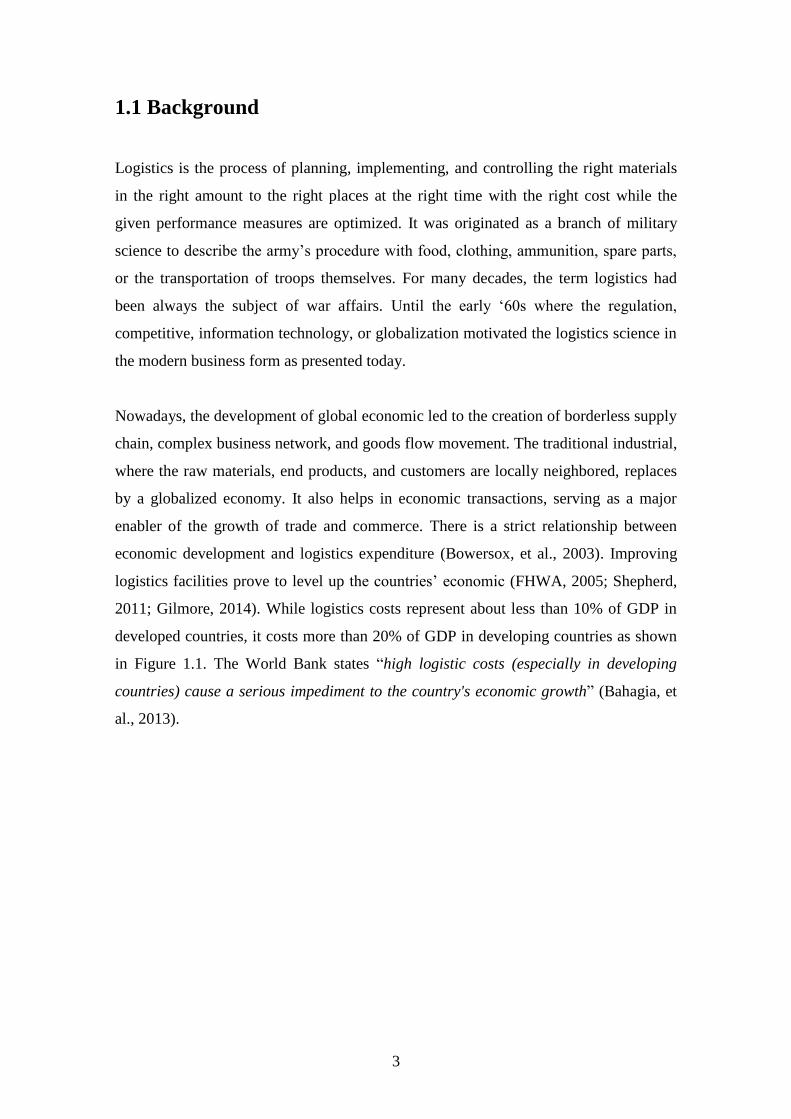
2011; Gilmore, 2014). While logistics costs represent about less than 10% of GDP in
developed countries, it costs more than 20% of GDP in developing countries as shown
in Figure 1.1. The World Bank states “high logistic costs (especially in developing
countries) cause a serious impediment to the country's economic growth” (Bahagia, et
al., 2013).
4
Figure 1.1 Relationship between Country GDP and Logistics Cost (Rodrigue, et al.,
2013)
To improve the logistics performance at a country level, the World Bank develops the
“Logistics Performance Index (LPI)” to help countries address the challenges and
opportunities they face in trade logistics. It guides what countries can do to improve
their performance (World Bank, 2015). The results based on the worldwide survey of
operators in every country and reflected both qualitative and quantitative measures. Six
key dimensions are weighted and represented the country’s LPI, including;
1. Efficiency of the clearance process by border control agencies, including the
Customs
2. Quality of trade and transport related infrastructure
3. Ease of arranging competitively priced shipments
4. Competence and quality of logistics services
5. Ability to track and trace consignments
Peru
Indonesia
India
Vietnam
Thailand
South Africa
China
Colombia
Mexico
Malaysia
Brazil Argentina
Chile
South Korea
Japan
France
Germany
Finland
Canada
United States
Singapore
Australia
0
5
10
15
20
25
30
35
0 10,000 20,000 30,000 40,000 50,000 60,000 70,000
Logis
tics C
ost (%
of G
DP
)
GDP per Capita (in current US dollars)
5
6. Timeliness of shipments in reaching the destination within the scheduled or
expected delivery time.
More results of the latest LPI including international LPI (i.e. global ranking and
country score card) and domestic LPI (i.e. environment and institutions, and
performance) present at www.lpi.worldbank.org.
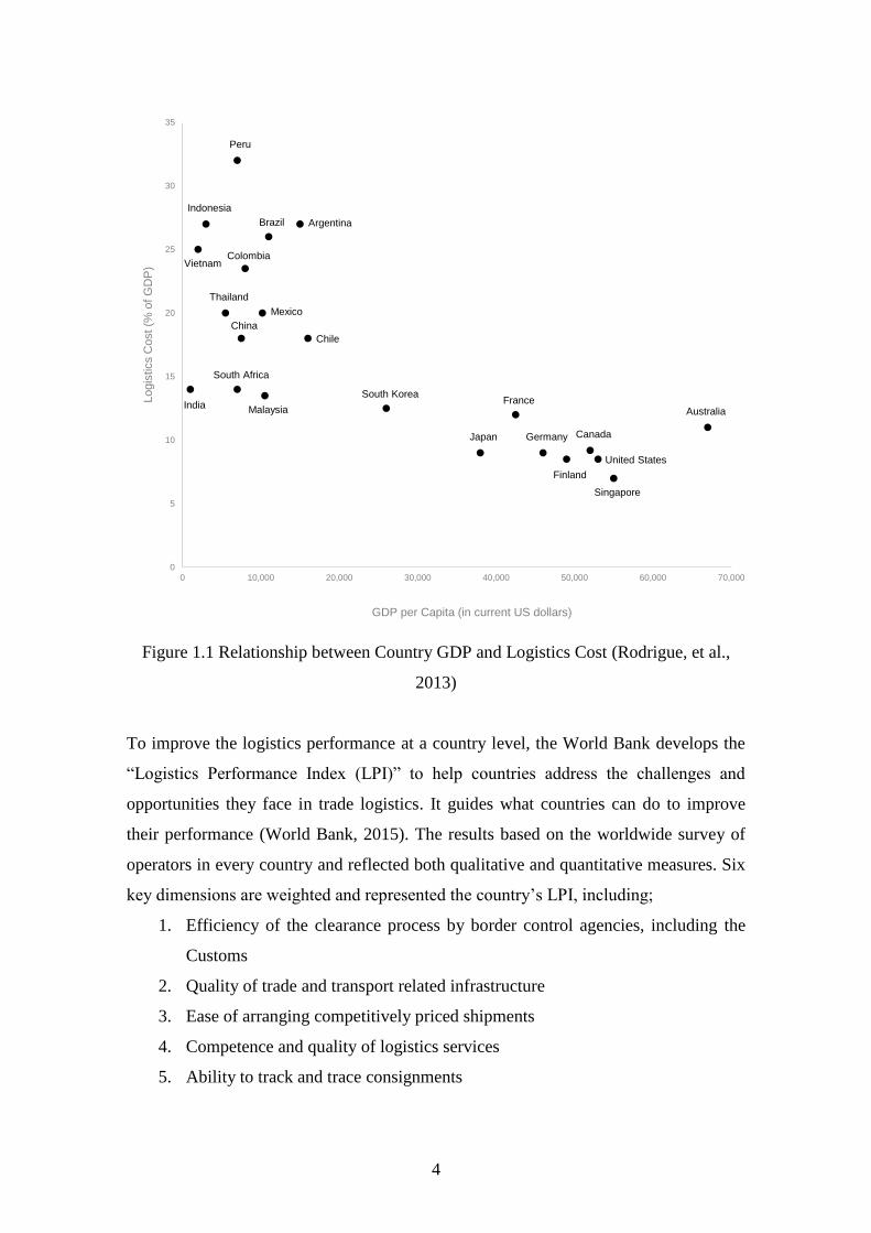
Considering the domestic level, the key activities of logistics that contribute to the total
cost include customer service, transportation, warehouse, inventory management, and
other processes (Figure 1.2). Transportation costs consist of inbound traveling costs
from the plants or suppliers to the warehouses/depots, and the outbound traveling costs
from the warehouses/depots to the customers. Warehousing costs are the fixed and
operating costs. The former is the combination of land acquisition, building, machinery,
maintenance, and administrative costs. The latter include labor, ordering, and material
handling (Srivastava, 1986). They are also essential to the effective coordinate and
completion of logistics task. The proportion of logistics cost depends on countries and
their economic. The logistics costs in the countries where economic rely on the natural
resource will generate higher logistic cost than the countries focusing on advanced
services (Rodrigue, et al., 2013). Three logistics strategies have to be fully addressed
and interrelated to achieve the customer service goal including location, inventory, and
transport decisions. Since there is a strong relationship among these logistics
components, reducing transportation cost might not only be achieved by improving
transportation features themselves (Ghiani, et al., 2013).
Figure 1.2 Worldwide Logistics Cost (Rodrigue, et al., 2013)
4%
6%
24%
27%
39%
Administration
Order Processing
Inventory Carrying
Warehousing
Transportation
6
The distribution network design is one of the most important strategic decision that
need to be optimized for the efficient long-term operation of whole supply chain. It
mostly involves all of the integrated decisions. The decisions made for network design
determine the number and locations of facility (i.e. factory, warehouse, or depot), select
the distribution channel to customers, and identify the transportation volume among
distributed facilities for an extended time horizon (Selim & Ozkarahan, 2008). This
problem usually involves making tradeoffs the cost components include the costs of
opening and operating the facility, and the transportation costs. These two cost
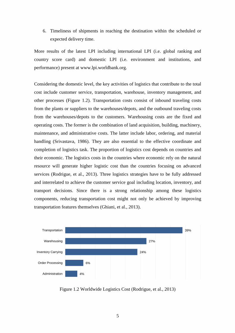
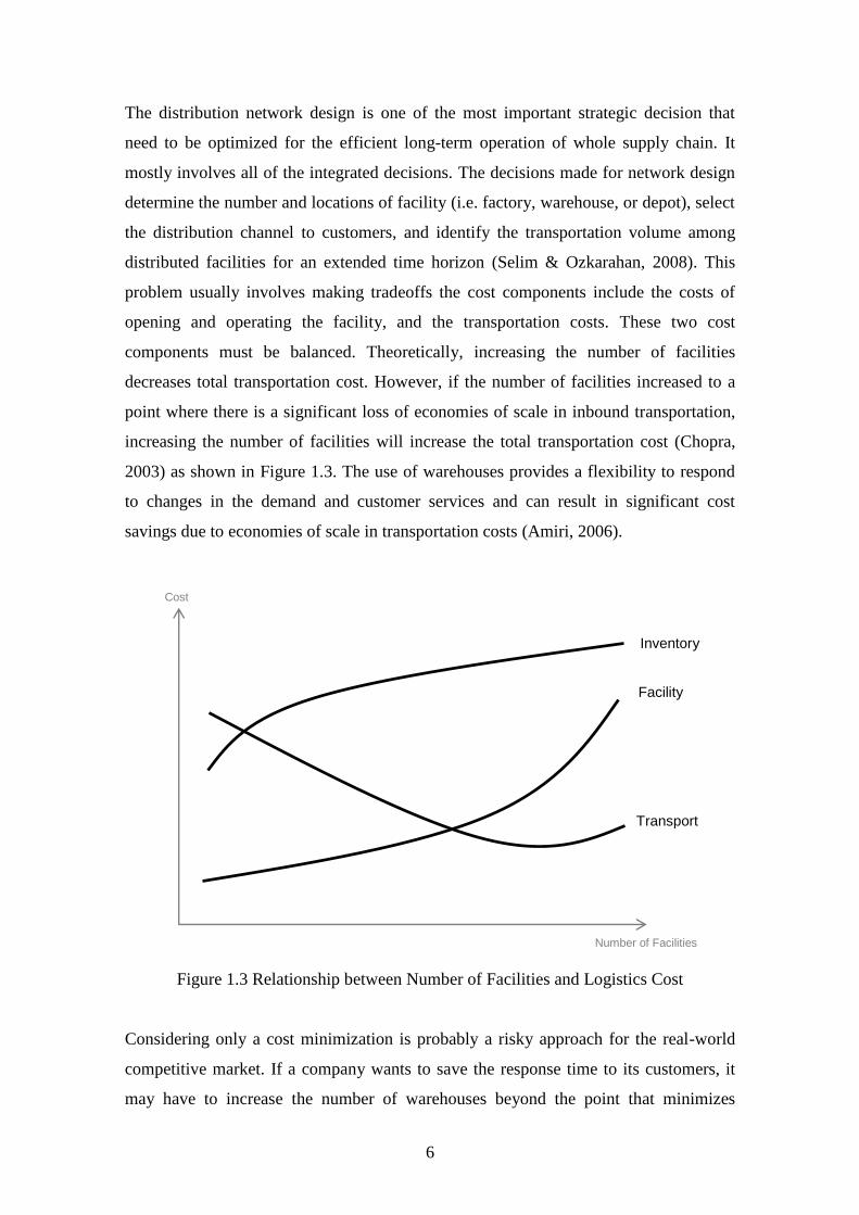
components must be balanced. Theoretically, increasing the number of facilities
decreases total transportation cost. However, if the number of facilities increased to a
point where there is a significant loss of economies of scale in inbound transportation,
increasing the number of facilities will increase the total transportation cost (Chopra,
2003) as shown in Figure 1.3. The use of warehouses provides a flexibility to respond
to changes in the demand and customer services and can result in significant cost
savings due to economies of scale in transportation costs (Amiri, 2006).
Figure 1.3 Relationship between Number of Facilities and Logistics Cost
Considering only a cost minimization is probably a risky approach for the real-world
competitive market. If a company wants to save the response time to its customers, it
may have to increase the number of warehouses beyond the point that minimizes
Number of Facilities
Cost
Inventory
Facility
Transport
7
logistics costs. Opening the new facilities that exceed the cost-minimizing point might
be required if such response increase in profit because of better responsiveness is
greater than the increase in costs of the additional facilities. For example, Amazon who
offers the customers to deliver the books within a week has only five stores. On the
other hand, Borders provided the books to their customers on that day needs to locate
more than 400 stores throughout the United States (Chopra, 2003).
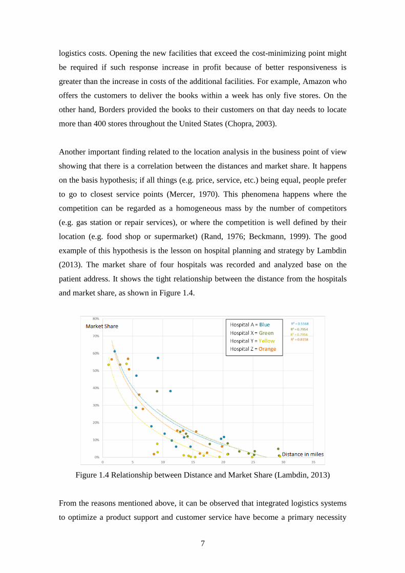
Another important finding related to the location analysis in the business point of view
showing that there is a correlation between the distances and market share. It happens
on the basis hypothesis; if all things (e.g. price, service, etc.) being equal, people prefer
to go to closest service points (Mercer, 1970). This phenomena happens where the
competition can be regarded as a homogeneous mass by the number of competitors
(e.g. gas station or repair services), or where the competition is well defined by their
location (e.g. food shop or supermarket) (Rand, 1976; Beckmann, 1999). The good
example of this hypothesis is the lesson on hospital planning and strategy by Lambdin
(2013). The market share of four hospitals was recorded and analyzed base on the
patient address. It shows the tight relationship between the distance from the hospitals
and market share, as shown in Figure 1.4.
Figure 1.4 Relationship between Distance and Market Share (Lambdin, 2013)
From the reasons mentioned above, it can be observed that integrated logistics systems
to optimize a product support and customer service have become a primary necessity
8
for private and public firms in the modern distribution management. Determining a
suitable location of the business center is one of the essential steps in supply chain
management. It involves in setting up factory, warehouse, retail store, or public
services, i.e. hospital, police station, fire station, etc. (Hassanzadeh, et al., 2009). It
involves the process to locate a set of facilities to minimize the cost of satisfying a set
of demands with respect to a set of constraints.
1.2 Research Motivation
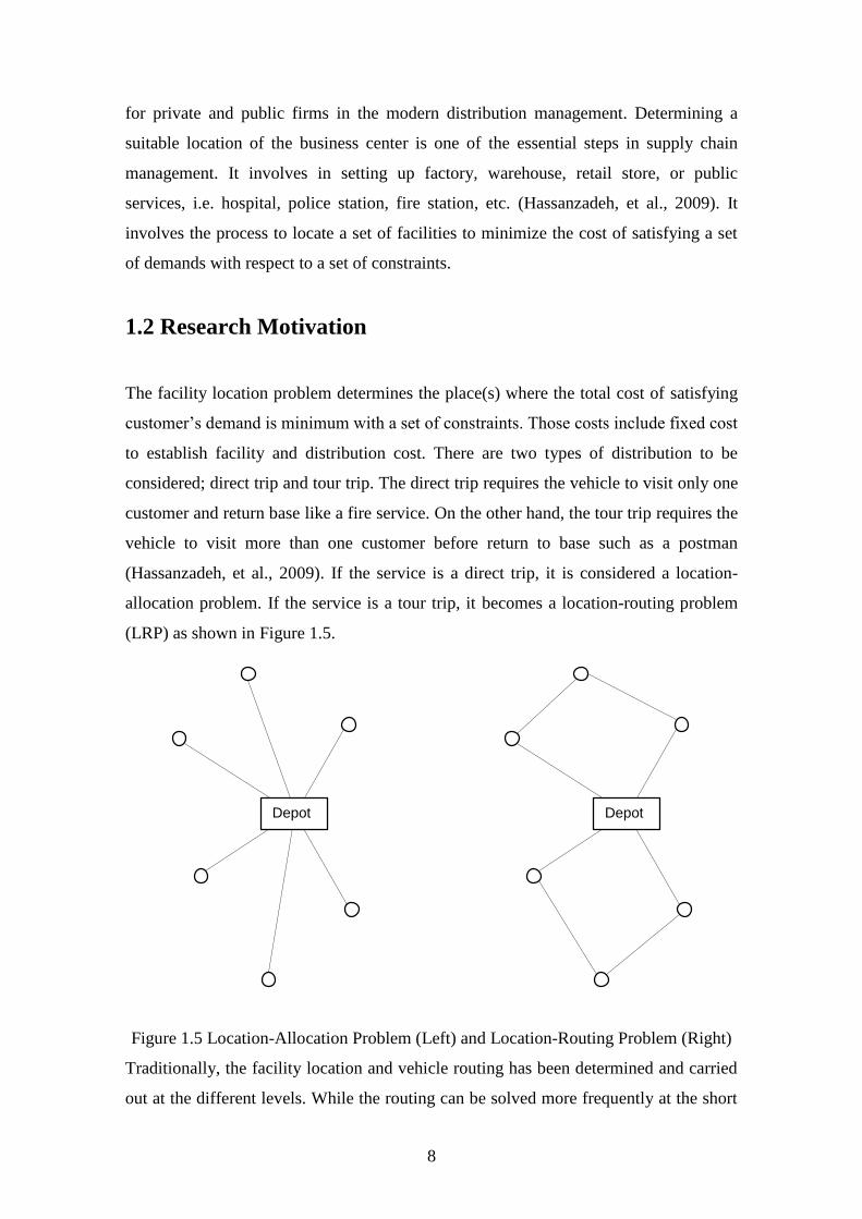
The facility location problem determines the place(s) where the total cost of satisfying
customer’s demand is minimum with a set of constraints. Those costs include fixed cost
to establish facility and distribution cost. There are two types of distribution to be
considered; direct trip and tour trip. The direct trip requires the vehicle to visit only one
customer and return base like a fire service. On the other hand, the tour trip requires the
vehicle to visit more than one customer before return to base such as a postman
(Hassanzadeh, et al., 2009). If the service is a direct trip, it is considered a location-
allocation problem. If the service is a tour trip, it becomes a location-routing problem
(LRP) as shown in Figure 1.5.
Figure 1.5 Location-Allocation Problem (Left) and Location-Routing Problem (Right)
Traditionally, the facility location and vehicle routing has been determined and carried
out at the different levels. While the routing can be solved more frequently at the short
Depot Depot
9
term operational stage, the facility must be located earlier in the long term strategic
planning. Some argue that an integration of these two problems, location and routing, is
impractical since they are in the different planning framework, which makes it
inappropriate to calculate them together.
Nagy and Salhi (2007) states three possible reasons why academics and practitioners
often ignore this interrelation and contribute to slow progress on the LRP. First, there
are many situations where the locational problems do not require a routing aspect.
Second, both decisions are in the different planning horizon. While the location is
strategic, the routing is a tactical problem. In other words, routes can be re-calculated
and re-drawn frequently, but depot locations are normally for a much longer period.
Thus, it is inappropriate to combine location and routing in the same planning
framework. Third, the LRP is conceptually more difficult than the classical location
problem. In the classical problems, the facility must be located by considering distances
to individual demand points. However, in LRP, the facility must be central about the
ensemble of the demand points as ordered by the (unknown) tour through all of them
(Berman, et al., 1995). Adding the routing into location problem adds difficulty in
solving these problems since there are far more decisions that need to be made by the
model.
These criticisms led the authors to investigate this issue. Eventually, it was proved that
the combination of location and routing problems reduces the cost over the long-term
horizon. Solving them together, early in the planning horizon provides benefits and
positive impacts for both operators and society (Rand, 1976; Salhi & Rand, 1989; Salhi
& Nagy, 1999). These decisions include (Marinakis, 2009):
How many facilities to locate?
Where is the location of facilities?
Which customers to assign to which depots?
Which customers to assign to which routes?
In what order of the customers should be on each route?
Moreover, in the context of logistics management, much attention has been paid to
improve the service quality by increasing customer satisfaction. It is recommended by
10
Min et al. (1998) that the future LRP studies should extend to consider the presence of
time windows since the customers often impose service deadlines and earliest service
time constraints. Some might argue that the delivery time is relatively small compared
to the time horizon of the facility location process. However, the technology
improvement enables the growth of a new market which responsive to customers’
behavior and their needs. On of them is the importance of “just in time” policies
(Gonzalez-Feliu, et al., 2012). The time windows are now almost essential to different
businesses such as bank deliveries, postal deliveries, industrial refuse collection, school
bus routing and scheduling, or the modern e-commerce (Solomon & Desrosiers, 1988).
According to the latest comprehensive surveys (Nagy & Salhi, 2007; Drexl &
Schneider, 2013; Prodhon & Prins, 2014), the LRP-related research are growing in
number. However, few of literature on location problem have been applied to specific
applications or case studies. The application-based publications are amount only less
than one-fifth (Nagy & Salhi, 2007). Current et al. (2002) summarized the reasons
behind this phenomenon. First, the application of location problem practices the
existing model and solution technique. It does not provide a scientific approach to
research literature. Second, the real world business and industries handle this task by
consultants or professional firms. They are not interested or motivated in sharing such
experiences. Third, the private sectors treat their valuable knowledge in this area
secretly. Nonetheless, it is still important to advance the modeling together with the
specific application in real world problem.
By adding the complexity of time window constraint into the LRP problem, a proper
and effective method must be developed to deal with its NP-hard (Dror, 1994). Despite
its importance, from our best knowledge of literature, all of the LRP studies that
considered time windows base on heuristic approaches. None of them attempted at the
optimal solution using the exact algorithm. Therefore, this study proposes the
integrated approach to determine the exact solution of the Location-Routing Problem
with Time Windows (LRPTW) using branch-and-price algorithm.
11
1.3 Research Purpose and Objectives
This study provides a broad scope for distribution network design to improve the
effectiveness of logistics processes. The main propose is to develop the integrated
model to consider the ordinary facility location problem (FLP) and vehicle routing
problem (VRP) simultaneously as the location-routing problem (LRP). The time
windows corresponding to the customer services is comprehensively considered as an
additional variant, lead the problem into the location-routing problem with time
windows (LRPTW) class. The objectives of this research are;
1. To formulate the mathematic models for LRPTW to minimize the total logistics
costs that consist of facility cost, vehicle cost, and transportation cost.
2. To set the new benchmarks of LRPTW and offers the optimal solutions.
3. To modify the supplementary heuristic approach to handling the large-scale
problems that extend the limitation of exact algorithms.
4. To demonstrate the application of developed models into the real world
problems. Distribution network and humanitarian logistics are selected as the
cases studies.
1.4 Research Contributions
This study is the first to solve the LRPTW to optimality using an exact algorithm.
We propose a branch-and-price approach with the fundamentals of column
generation together with the Elementary Shortest Path Problem with Resource
Constraint as a pricing problem.
The acceleration processes are developed to reduce the search space and improve
computational time and resources.
The new test instances of the LRPTW are formulated from the original VRPTW
Solomon benchmark instances to evaluate the performance of our algorithm. To this
end, additional depot locations are generated by using the k-medoids algorithm. The
resulting instances are expected to be the new benchmarks for other researchers.
12
The computational results and the corresponding discussion to understand the
effects and characteristics of time window constraints in the LRPTW is another
scientific contribution.
The impact of the main parameters in logistics costs is evaluated from freight
carrier with different depot location, depot size, and vehicle size.
The LRPTW model is applied to the humanitarian logistics to determine the
locations of the depots as the centers for disaster relief operation. The city of
Ishinomaki which attacked by the tsunami triggered by the great Japanese
earthquake on March 11, 2011, is selected as a case study.
1.5 Research Outlines
This chapter describes the broad introduction about the situation of supply chain and
logistics management systems. The cost components of transportation, warehousing,
inventory, order processing, and administration are explored. The research motivation
for location analysis is introduced. It leads to the purpose and objectives of this
research, together with the lists of research contributions.
Chapter 2 reviews the literature related to this research. Two types of location problems
are described which are a location on a continuous plane and location on a network.
The integration between location and routing problems is comprehensively described
with the exact solution methods. The details related to time windows and benchmark
instances give are also provided.
Chapter 3 presents the main formulation of LRPTW. The objective function and eleven
constraints are described in details. The branch-and-price algorithm is as a main tool to
solve LRPTW. It consists of a master problem, subproblem, accelerating processes, and
branching strategies. The results and effects of time windows on testing instances,
developed from VRPTW Solomon benchmarks, are shown in Chapter 4. It describes
the cost components including the depot, vehicle, distance, load, and computational
time.
13
The application of LRPTW is applied in Osaka distribution network and Ishinomaki
humanitarian logistics, as presented in Chapter 5 and Chapter 6, respectively. Although
the background of these two problems is different, the main purpose remains the same.
The model determines the best locations for the depots, the number of vehicles, the
sequence of the demand points, and the best routes to deliver goods. Numbers of
scenarios are evaluated based on the different cost components and other constraints.
Finally, the conclusions of this research are summarized, and extensions to this research
presents in Chapter 7.
14
References
Amiri, A., 2006. Designing a distribution network in a supply chain system:
Formulation and efficient solution procedure. European Journal of Operational
Research, 171(2), p. 567–576.
Bahagia, I., Senator, N., Sandee, H. & Meeuws, R., 2013. State of Logistics Indonesia
2013, Washington DC: World Bank.
Beckmann, M. J., 1999. Market Areas. In: Lectures on Location Theory. Berlin:
Springer Berlin Heidelberg, pp. 13-20.
Berman, O., Jaillet, P. & Simchi-Levi, D., 1995. Location-routing problems with
uncertainty. In: Z. Drezner, ed. Facility Location: A Survey of Applications and
Methods. New York: Springer, pp. 427-452.
Bowersox, D. J., Calantone, R. J. & Rodrigues, A. M., 2003. Estimation of global
logistics expenditures using neural networks. Journal of Business Logistics, 24(2),
pp. 21-36.
Chopra, S., 2003. Designing the distribution network in a supply chain. Transportation
Research, 39(2), pp. 123-140.
Current, J., Daskin, M. & Schilling, D., 2002. Discrete network location models. In: Z.
Drezner & H. Hamacher, eds. Facility Location: Applications and Theory. Berlin:
Springer, pp. 81-108.
Drexl, M. & Schneider, M., 2013. A survey of location-routing problems, Mainz:
Johannes Gutenberg University.
Dror, M., 1994. Note on the complexity of the shortest path models for column
generation in VRPTW. Operations Research, 42(5), pp. 977-978.
FHWA, 2005. Logistics Costs and U.S. Gross Domestic Product, Washington DC:
Federal Highway Administration.
Ghiani, G., Laporte, G. & Musmanno, R., 2013. Introduction to logistics systems
management. West Sussex: John Wiley & Sons, Ltd.
Gilmore, D., 2014. State of the Logistics Union 2014. [Online] Available at:
http://www.scdigest.com/ASSETS/FIRSTTHOUGHTS/14-06-17.php?cid=8190
[Accessed 30 4 2015].
15
Gonzalez-Feliu, J., Ambrosini, C. & Routhier, J. L., 2012. New trends on urban goods
movement: Modelling and simulation of e-commerce distribution. European
Transport, Volume 50, p. 23.
Hassanzadeh, A. et al., 2009. Location-Routing Problem. In: R. Zanjirani Farahani &
M. Hekmatfar, eds. Facility Location: Concepts, Models, Algorithms and Case
Studies. Heidelberg: Springer.
Lambdin, L. A., 2013. What Drives Market Share? Distance Matters!. [Online]
Available at: http://www.stratasan.com/what-drives-market-share-distance-matters/
[Accessed 9 5 2015].
Marinakis, Y., 2009. Location Routing Problem. In: C. A. Floudas & P. M. Pardalos,
eds. Encyclopedia of Optimization. New York: Springer US, pp. 1919-1925.
Mercer, A., 1970. Strategic planning of physical distribution systems. International
Journal of Physical Distribution, 1(1), pp. 20-25.
Min, H., Jayaraman, V. & Srivastara, R., 1998. Combined location-routing problem: A
synthesis and future research directions. European Journal of Operational
Research, 108(1), pp. 1-15.
Nagy, G. & Salhi, S., 2007. Location-Routing: Issues, Models, and Methods. European
Journal of Operational Research, Volume 177, pp. 649-672.
Prodhon, C. & Prins, C., 2014. A survey of recent research on location-routing
problems. European Journal of Operational Research, 238(1), pp. 1-17.
Rand, G., 1976. Methodological Choices in Depot Location Studies. Operational
Research Quarterly, Volume 27, pp. 241-249.
Rodrigue, J. P., Comtois, C. & Slack, B., 2013. The Geography of Transport Systems. 3
ed. s.l.:Routledge.
Salhi, S. & Nagy, G., 1999. Consistency and Robustness in Location-Routing. Studies
in Locational Analysis, Volume 13, pp. 3-19.
Salhi, S. & Rand, G., 1989. The Effect of Ignoring Routes when Locating Depots.
European Journal of Operation Research, Volume 39, pp. 150-156.
Selim, H. & Ozkarahan, I., 2008. A supply chain distribution network design model: an
interactive fuzzy goal programming-based solution approach. The International
Journal of Advanced Manufacturing Technology, Volume 36, pp. 401-418.
Shepherd, B., 2011. Logistics costs and competitiveness: Measurement and trade policy
applicatoins, Washington DC: World Bank.
16
Solomon, M. M. & Desrosiers, J., 1988. Survey Paper - Time Window Constrained
Routing and Scheduling Problems. Transportation Science, 22(1), pp. 1-13.
Srivastava, R., 1986. Algorithms for solving the location-routing problem, The Ohio
State University: Doctoral dissertation.
World Bank, 2015. Logistics Performance Index. [Online] Available at:
http://lpi.worldbank.org/ [Accessed 30 4 2015].
17
Chapter 2
Literature Review
2.1 Facility Location Problem
2.1.1 Location on a Continuous Plane
2.1.2 Location on a Network
2.2 Location-Routing Problem
2.3 Exact Methods in LRP
2.4 Column Generation
2.5 Time Windows
2.6 Benchmark Instances
References

18
19
2.1 Facility Location Problem
The facility location problem is a branch of operation research on location analysis. The
aim is to determine the optimal location of the facility to minimize transport cost. In
general, there are two types of main structural categories (Eilon, et al., 1971). The first
approach is an infinite set approach or location on a continuous plane. It allows no
restrictions as to where are the location of the depots. The objective is to find the location
of facilities that minimize the sum of weighted distances of customers from these
locations. The second approach is a feasible set approach or location on a network. This
type of problem considers a finite solution space that consist of points on the network
and specify a list of possible depot locations.
In transportation and logistics modeling, one of the most fundamental data used in the
design, analysis, and operation is the distance. One might think that the most accuracy
distance is the actual road distance driven by the actual vehicle. However, the
approximated distance is still required in the recent algorithm since the actual road
distance is too expensive or even unknown (Goetschalckx, 2011). Nowadays, three types
of distances are still widely used to compute the distance between points in a plane which
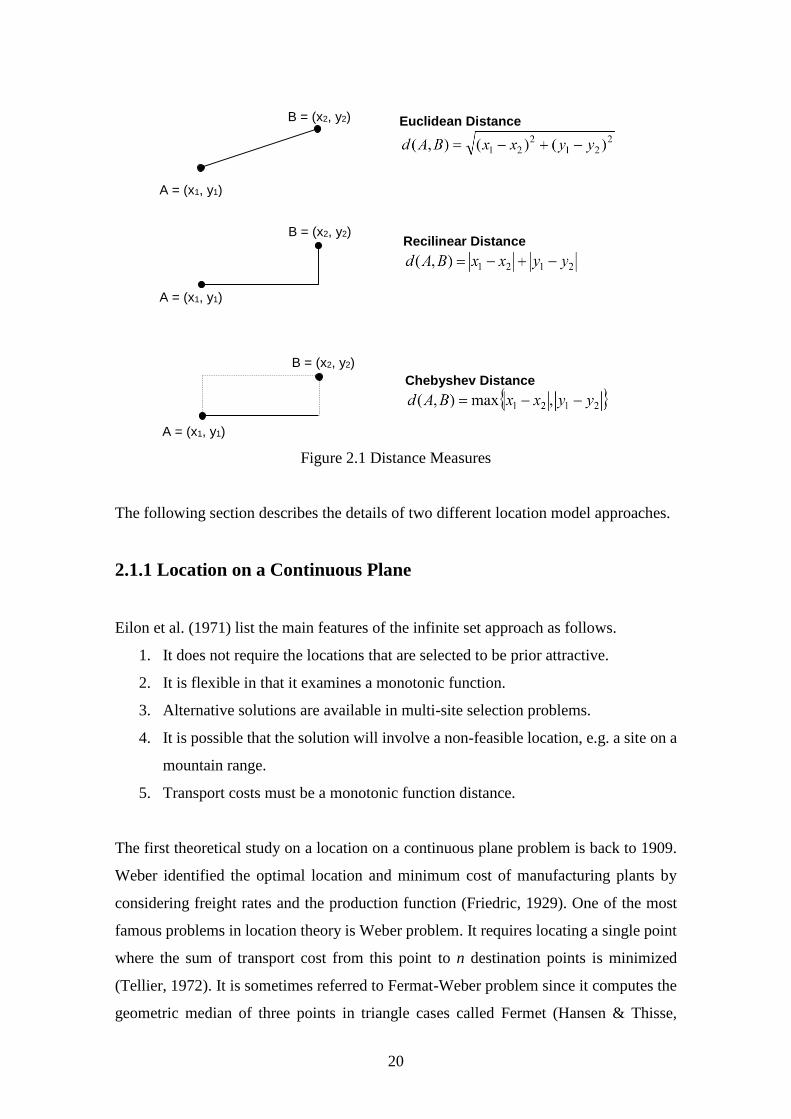
are Euclidean, Rectilinear, and Chebyshev (Figure 2.1). The Euclidean distance is also
called the straight line distance, frequently used in a global or national level where
approximate distances are acceptable. It is widely used in the communications industry.
The Rectilinear Distance is primarily used in transportation and logistics firms where the
distance measures on perpendicular and cross lines, represented the grid roads in the
cities. Lastly, the Chebyshev distance is also called the simultaneous travel distance, used
in material handling process where vertical movement is involved.
20
Figure 2.1 Distance Measures
The following section describes the details of two different location model approaches.
2.1.1 Location on a Continuous Plane
Eilon et al. (1971) list the main features of the infinite set approach as follows.
1. It does not require the locations that are selected to be prior attractive.
2. It is flexible in that it examines a monotonic function.
3. Alternative solutions are available in multi-site selection problems.
4. It is possible that the solution will involve a non-feasible location, e.g. a site on a
mountain range.
5. Transport costs must be a monotonic function distance.
The first theoretical study on a location on a continuous plane problem is back to 1909.
Weber identified the optimal location and minimum cost of manufacturing plants by
considering freight rates and the production function (Friedric, 1929). One of the most
famous problems in location theory is Weber problem. It requires locating a single point
where the sum of transport cost from this point to n destination points is minimized
(Tellier, 1972). It is sometimes referred to Fermat-Weber problem since it computes the
geometric median of three points in triangle cases called Fermet (Hansen & Thisse,
A = (x1, y1)
B = (x2, y2)
A = (x1, y1)
B = (x2, y2)
A = (x1, y1)
B = (x2, y2)
Euclidean Distance
Recilinear Distance
Chebyshev Distance
21
1983). The classical problems in location analysis are set covering location problem
(Toregas, et al., 1971), the maximum covering location problem (Church & ReVelle,
1974), p-median and p-center problems (Hakimi, 1964), and uncapacitated facility
location problem (Kuehn & Hamburger, 1963). The more complex problem in this
discipline in the multi-facility location problem. Two techniques that are widely used in
location theory is minisum and minimax. Minisum facility location determines the
minimizing the sum of the weighted distance between the new facility and the other
existing facilities. Minimax location problem calculates the minimizing the maximum
distance between the new facility and any existing facility.
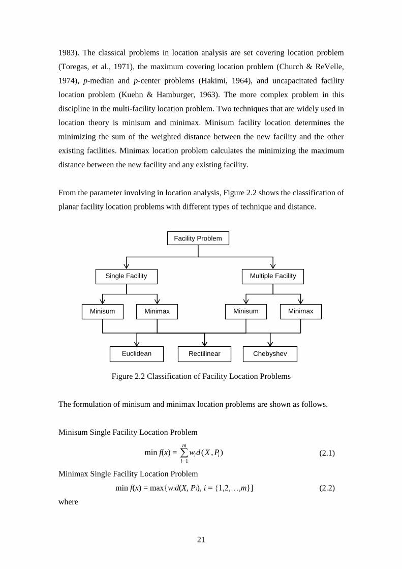
From the parameter involving in location analysis, Figure 2.2 shows the classification of
planar facility location problems with different types of technique and distance.
Figure 2.2 Classification of Facility Location Problems
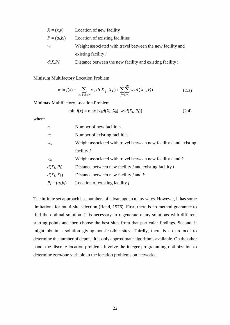
The formulation of minisum and minimax location problems are shown as follows.
Minisum Single Facility Location Problem
min f(x) =
m
iii PXdw
1
),( (2.1)
Minimax Single Facility Location Problem
min f(x) = max{wid(X, Pi), i = {1,2,…,m}] (2.2)
where
Facility Problem
Single Facility Multiple Facility
Minisum Minimax Minisum Minimax
Rectilinear Euclidean Chebyshev
22
X = (x,y) Location of new facility
P = (ai,bi) Location of existing facilities
wi Weight associated with travel between the new facility and
existing facility i
d(X,Pi) Distance between the new facility and existing facility i
Minisum Multifactory Location Problem
min f(x) =
nkj
n
j
m
iijjikjjk PXdwXXdv
1 1 1
),(),( (2.3)
Minimax Multifactory Location Problem
min f(x) = max{vjkd(Xj, Xk), wjid(Xj, Pi)} (2.4)
where
n Number of new facilities
m Number of existing facilities
wij Weight associated with travel between new facility i and existing
facility j
vik Weight associated with travel between new facility i and k
d(Xj, Pi) Distance between new facility j and existing facility i
d(Xj, Xk) Distance between new facility j and k
Pj = (aj,bj) Location of existing facility j
The infinite set approach has numbers of advantage in many ways. However, it has some
limitations for multi-site selection (Rand, 1976). First, there is no method guarantee to
find the optimal solution. It is necessary to regenerate many solutions with different
starting points and then choose the best sites from that particular findings. Second, it
might obtain a solution giving non-feasible sites. Thirdly, there is no protocol to
determine the number of depots. It is only approximate algorithms available. On the other
hand, the discrete location problems involve the integer programming optimization to
determine zero/one variable in the location problems on networks.
23
2.1.2 Location on a Network
Eilon et al. (1971) list the main features of the feasible set approach as follows.
1. It incorporates costs that relate to specific geographic locations.
2. It does not require transport costs to be any function of distance.
3. It requires a set of sites that are known to be feasible and for which all cost data
are available.
4. The number of locations must be finite and sufficiently small for computational
efficiency.
5. The set of feasible sites may not include the optimum solution.
The comprehensive study on network-based location problem started in the middle of
1960s. Hakimi (1964) and Hakimi (1965) investigated the minimum weighted distance
location of p facilities on a network of n demand nodes and named the p-median problem.
His works were similar to the linear programming proposed by Dantzig by reducing the
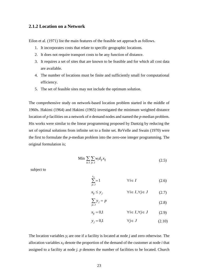
set of optimal solutions from infinite set to a finite set. ReVelle and Swain (1970) were
the first to formulate the p-median problem into the zero-one integer programming. The
original formulation is;
Min Ii Jj
ijiji xdw (2.5)
subject to
ijx
Jj
1 Ii (2.6)
jij yx JjIi , (2.7)
Jj
j py (2.8)
1,0ijx JjIi , (2.9)
1,0jy Jj (2.10)
The location variables yj are one if a facility is located at node j and zero otherwise. The
allocation variables xij denote the proportion of the demand of the customer at node i that
assigned to a facility at node j. p denotes the number of facilities to be located. Church
24
and ReVelle (1976) reported one of the important way to measure the effectiveness of
facility location is to determine the average distance traveled by vehicles. Later, Kariv
and Hakimi (1979) proved that the general p-median problem in NP-Hard.
The first heuristic solution to apply in the p-median problem called location-allocation
heuristics, introduced by Maranzana (1964) and following by the more powerful vertex
substation technique of Teitz and Bart (1968). They are the earliest simultaneously
exchanged algorithms that lately called 1-opt heuristics. Although the simplex algorithm
of 1-opt lead to the optimal solution, this work does not always produce the global
optimum since the solution space of p-median is not necessary convex. Galvão (1993)
employed the exact solution by applying Lagrangian relaxation and the linear
programming relaxation. The heuristics concentration is introduced by Rosing and
ReVelle (1997) incorporated the exchange heuristics in metaheuristics. Lately, it was
proved by Schilling et al. (2000) that the performance of both exact and heuristic
solutions of p-median problem depends on the extent of the triangle inequality is
determined underlying the problem.
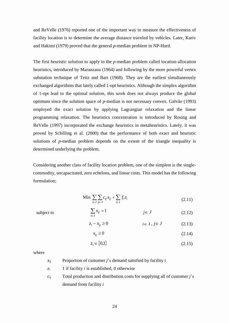
Considering another class of facility location problem, one of the simplest is the single-
commodity, uncapacitated, zero echelons, and linear costs. This model has the following
formulation;
Min
Ii Jj Ii
iiijij zfxc (2.11)
subject to 1Ii
ijx Jj (2.12)
0 iji xz Ii , Jj (2.13)
0ijx (2.14)
1,0iz (2.15)
where
xij Proportion of customer j’s demand satisfied by facility i
zi 1 if facility i is established, 0 otherwise
cij Total production and distribution costs for supplying all of customer j’s
demand from facility i
25
fi Fixed cost of establishing facility i
I, J Sets of candidate facility sites and customer zones, respectively
Constraints (2.12) ensure that each customer’s demand is satisfied exactly and
Constraints (2.13) confirm that customers visits by vehicles from open facilities only.
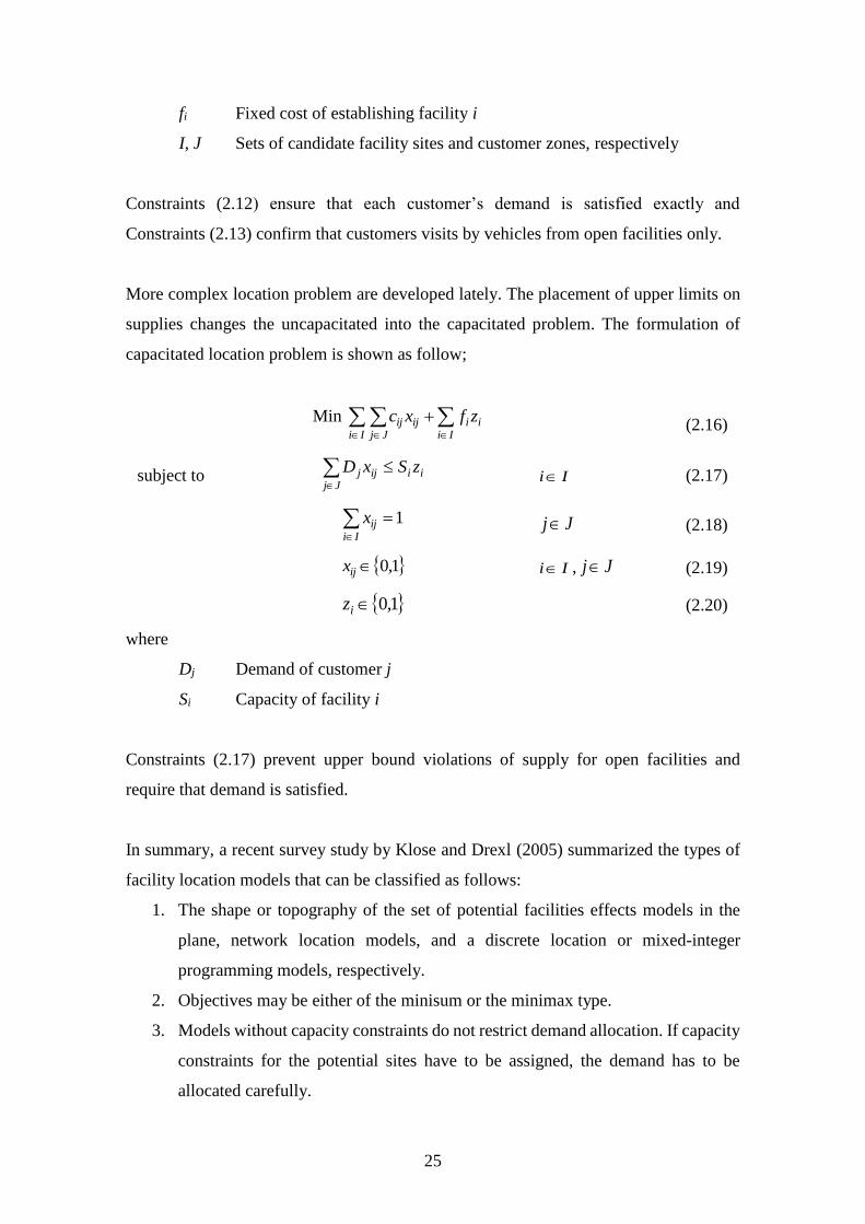
More complex location problem are developed lately. The placement of upper limits on
supplies changes the uncapacitated into the capacitated problem. The formulation of
capacitated location problem is shown as follow;
Min
Ii Jj Ii
iiijij zfxc (2.16)
subject to iiJj
ijj zSxD
Ii (2.17)
1Ii
ijx Jj (2.18)
1,0ijx Ii , Jj (2.19)
1,0iz (2.20)
where
Dj Demand of customer j
Si Capacity of facility i
Constraints (2.17) prevent upper bound violations of supply for open facilities and
require that demand is satisfied.
In summary, a recent survey study by Klose and Drexl (2005) summarized the types of
facility location models that can be classified as follows:
1. The shape or topography of the set of potential facilities effects models in the
plane, network location models, and a discrete location or mixed-integer
programming models, respectively.
2. Objectives may be either of the minisum or the minimax type.
3. Models without capacity constraints do not restrict demand allocation. If capacity
constraints for the potential sites have to be assigned, the demand has to be
allocated carefully.
26
4. Single-stage models focus on distribution systems covering only one stage
explicitly. In multi-stage models, the flow of goods comprising several
hierarchical stages has to be examined.
5. Single-product models can be considered by the fact that demand, cost, and
capacity for several products can be aggregated to a single homogeneous product.
6. Location models base on the assumption that demand is inelastic, meaning that
demand is independent of spatial decisions.
7. Static models try to optimize the objective function for one representative period.
By contrast, dynamic models reflect data varying over time within a given
planning horizon.
8. In practice, data are based on forecasts and are likely to be uncertain. As a
consequence, we have either deterministic models if the input is known with
certainty or probabilistic models if the input is subject to uncertainty.
9. In classical models, the quality of demand allocation is measured in isolation for
each pair of supply and demand points. Unfortunately, if demand is satisfied
through delivery tours, the delivery cost cannot be calculated for each pair of
supply and demand points separately. The combination of location and routing
models elaborate on this interrelationship.
2.2 Location-Routing Problem
The definition of location-routing problem (LRP) given by Srivastava and Benton (1990)
states as:
“Given a feasible set of potential depot sites and customer sites, find the
location of the depots and the routes to customers from the depots such
that the overall cost is minimized. The overall cost is the sum of the
location and distribution costs.”
From the previous topic, the facility location problem does not require a routing
determination, similar to the p-median problems. Likewise, the multi-depot vehicle
routing problem does not solve the facility location since it is implicitly determined.
However, in the LRP, two decisions are considered interdependently, how many and
which facilities should be opened and which routes should be built to meet customer
27
demand. The former is based on ordinary location problem while the latter is developed
with the fundamentals of the vehicle-routing problem (VRP) seeking to serve a set of
customers with a fleet of vehicles with minimum distribution cost.
One of the first study that pointed out the important of routing in location problem
referred to Maranzana (1964). This study stated that “the location of factories,
warehouses and supply points in general … is often influenced by transport costs”.
Lately, Rand (1976) observed “many practitioners are aware of the danger of sub-
optimizing by separating depot location and vehicle routing.” Watson-Gandy and Dohrn
(1973) is probably one of the first studies to consider the tour of the vehicle routes within
the location-transportation framework. Until then, the consideration to integrate the
routing in location analysis became more popular among researchers. It includes Or and
Pierskalla (1979), Jacobsen and Madsen (1978), Harrison (1979), Jacobsen and Madsen
(1980), Nambiar et al. (1981), Laporte and Nobert (1981), and Madsen (1983).
One of the early works published by Rand (1976). He pointed out that the practitioners
should be aware of the danger of sub-optimizing by separating depot location and vehicle
routing since the best vehicle routes are not necessarily the one that minimize the distance
traveled. However, it is difficult to incorporate routing in depot locations analysis at that
time because of the shortage of computational resources. Lately, Salhi and Rand (1989)
evaluated the effect of ignoring routing when locating the depots by using a two stage
process. This study proved that the best solution after the location stage does not
necessarily produce the lowest transport cost after the routing stages. This result was
found both when compare the best locations obtained from various methods, and when
evaluate a single method for different numbers of depots. Salhi and Nagy (1999)
developed the work on location-routing heuristics using location-first routing-second
methods. Their work proved that the combined models consistently produce a solution
of higher quality than sequential methods.
Larporte and Nobert (1981) is among the first authors to formulate the simple
uncapacitated LRP model by a global integer programming that require opening only one
single depot. No vehicle costs are considered. Later on, most authors address the LRP
with capacity constraints on depots and vehicles and vehicle cost which called
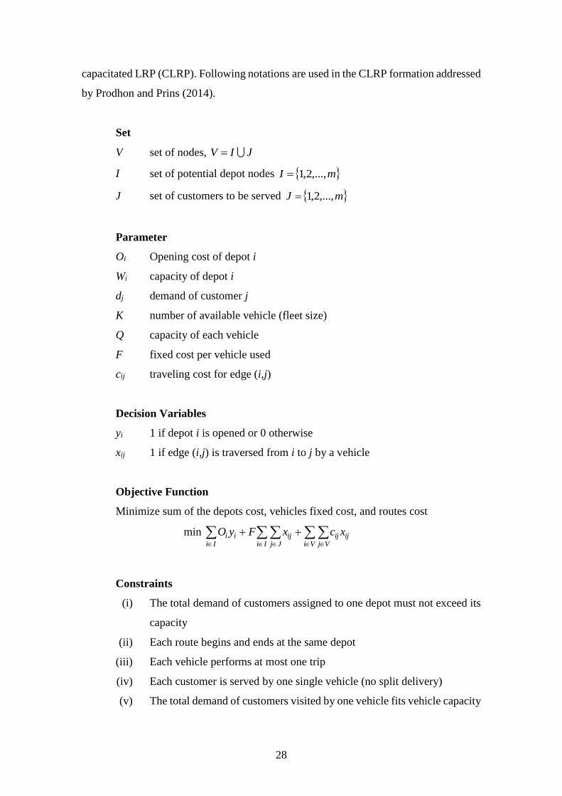
28
capacitated LRP (CLRP). Following notations are used in the CLRP formation addressed
by Prodhon and Prins (2014).
Set
V set of nodes, JIV
I set of potential depot nodes mI ,...,2,1
J set of customers to be served mJ ,...,2,1
Parameter
Oi Opening cost of depot i
Wi capacity of depot i
dj demand of customer j
K number of available vehicle (fleet size)
Q capacity of each vehicle
F fixed cost per vehicle used
cij traveling cost for edge (i,j)
Decision Variables
yi 1 if depot i is opened or 0 otherwise
xij 1 if edge (i,j) is traversed from i to j by a vehicle
Objective Function
Minimize sum of the depots cost, vehicles fixed cost, and routes cost
min
Vi Vj
ijijIi Jj
ijIi
ii xcxFyO
Constraints
(i) The total demand of customers assigned to one depot must not exceed its
capacity
(ii) Each route begins and ends at the same depot
(iii) Each vehicle performs at most one trip
(iv) Each customer is served by one single vehicle (no split delivery)
(v) The total demand of customers visited by one vehicle fits vehicle capacity
29
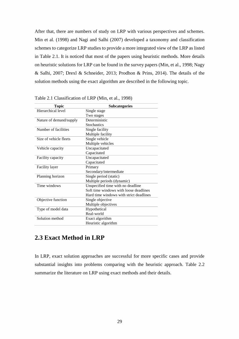
After that, there are numbers of study on LRP with various perspectives and schemes.
Min et al. (1998) and Nagi and Salhi (2007) developed a taxonomy and classification
schemes to categorize LRP studies to provide a more integrated view of the LRP as listed
in Table 2.1. It is noticed that most of the papers using heuristic methods. More details
on heuristic solutions for LRP can be found in the survey papers (Min, et al., 1998; Nagy
& Salhi, 2007; Drexl & Schneider, 2013; Prodhon & Prins, 2014). The details of the
solution methods using the exact algorithm are described in the following topic.
Table 2.1 Classification of LRP (Min, et al., 1998)
Topic Subcategories
Hierarchical level Single stage
Two stages
Nature of demand/supply Deterministic
Stochastics
Number of facilities Single facility
Multiple facility
Size of vehicle fleets Single vehicle
Multiple vehicles
Vehicle capacity Uncapacitated
Capacitated
Facility capacity Uncapacitated
Capacitated
Facility layer Primary
Secondary/intermediate
Planning horizon Single period (static)
Multiple periods (dynamic)
Time windows Unspecified time with no deadline
Soft time windows with loose deadlines
Hard time windows with strict deadlines
Objective function Single objective
Multiple objectives
Type of model data Hypothetical
Real-world
Solution method Exact algorithm
Heuristic algorithm
2.3 Exact Method in LRP
In LRP, exact solution approaches are successful for more specific cases and provide
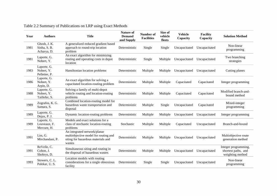
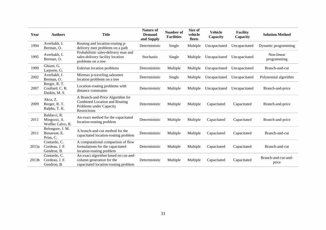
substantial insights into problems comparing with the heuristic approach. Table 2.2
summarize the literature on LRP using exact methods and their details.
30
Table 2.2 Summary of Publications on LRP using Exact Methods
Year Authors Title
Nature of
Demand
and Supply
Number of
Facilities
Size of
vehicle
fleets
Vehicle
Capacity
Facility
Capacity Solution Method
1981
Ghosh, J. K.
Sinha, S. B.
Acharya, D.
A generalized reduced gradient based
approach to round-trip location
problem
Deterministic Single Single Uncapacitated Uncapacitated Non-linear
programming
1981 Laporte, G.
Nobert, Y.
An exact algorithm for minimizing
routing and operating costs in depot
location
Deterministic Single Multiple Uncapacitated Uncapacitated Two branching
strategies
1983
Laporte, G.
Nobert, Y.
Pelletier, P.
Hamiltonian location problems Deterministic Multiple Multiple Uncapacitated Uncapacitated Cutting planes
1986
Laporte, G.
Nobert, Y.
Arpin, D.
An exact algorithm for solving a
capacitated location-routing problem Deterministic Multiple Multiple Capacitated Capacitated Integer programming
1988
Laporte, G.
Nobert, Y.
Taillefer, S.
Solving a family of multi-depot
vehicle routing and location-routing
problems
Deterministic Multiple Multiple Capacitated Capacitated Modified branch-and-
bound method
1989 Zografos, K. G.
Samara, S.
Combined location-routing model for
hazardous waste transportation and
disposal
Deterministic Multiple Single Uncapacitated Capacitated Mixed-integer
programming
1989 Laporte, G.
Dejax, P. J. Dynamic location-routing problems Deterministic Multiple Multiple Uncapacitated Uncapacitated Integer programming
1989
Laporte, G.
Louveaux, F.
Mercure, H.
Models and exact solutions for a
class of stochastic location-routing
problems
Stochastic Multiple Multiple Capacitated Uncapacitated Branch-and-bound
1991 List, G.
Mirchandani, P.
An integrated network/planar
multiobjective model for routing and
siting for hazardous materials and
wastes
Deterministic Multiple Multiple Uncapacitated Uncapacitated Multiobjective route
generation method
1991
ReVelle, C.
Cohon, J.
Shobrys, D.
Simultaneous siting and routing in
the disposal of hazardous wastes Deterministic Multiple Multiple Uncapacitated Uncapacitated
Integer programming,
shortest paths, and
weighting method
1993 Stowers, C. L.
Palekar, U. S.
Location models with routing
considerations for a single obnoxious
facility
Deterministic Single Single Uncapacitated Uncapacitated Non-linear
programming
31
Year Authors Title
Nature of
Demand
and Supply
Number of
Facilities
Size of
vehicle
fleets
Vehicle
Capacity
Facility
Capacity Solution Method
1994 Averbakh, I.
Berman, O.
Routing and location-routing p-
delivery men problems on a path Deterministic Single Multiple Uncapacitated Uncapacitated Dynamic programming
1995 Averbakh, I.
Berman, O.
Probabilistic sales-delivery man and
sales-delivery facility location
problems on a tree
Stochastic Single Multiple Uncapacitated Uncapacitated Non-linear
programming
1999 Ghiani, G.
Larporte, G. Eulerian location problems Deterministic Multiple Multiple Uncapacitated Uncapacitated Branch-and-cut
2002 Averbakh, I.
Berman, O.
Minmax p-traveling salesmen
location problems on a tree Deterministic Single Multiple Uncapacitated Uncapacitated Polynomial algorithm
2007
Berger, R. T.
Coullard, C. R.
Daskin, M. S.
Location-routing problems with
distance constraints Deterministic Multiple Multiple Uncapacitated Uncapacitated Branch-and-price
2009
Akca, Z.
Berger, R. T.
Ralphs, T. K.
A Branch-and-Price Algorithm for
Combined Location and Routing
Problems under Capacity
Restrictions
Deterministic Multiple Multiple Capacitated Capacitated Branch-and-price
2011
Baldacci, R.
Mingozzi, A.
Wolfler Calvo, R.
An exact method for the capacitated
location-routing problem Deterministic Multiple Multiple Capacitated Capacitated Branch-and-price
2011
Belengure, J. M.
Benavent, E.
Prins, C.
A branch-and-cut method for the
capacitated location-routing problem Deterministic Multiple Multiple Capacitated Capacitated Branch-and-cut
2013a
Contardo, C.
Cordeau, J. F.
Gendron, B.
A computational comparison of flow
formulations for the capacitated
location-routing problem
Deterministic Multiple Multiple Capacitated Capacitated Branch-and-cut
2013b
Contardo, C.
Cordeau, J. F.
Gendron, B.
An exact algorithm based on cut-and-
column generation for the
capacitated location-routing problem
Deterministic Multiple Multiple Capacitated Capacitated Branch-and-cut-and-
price
32
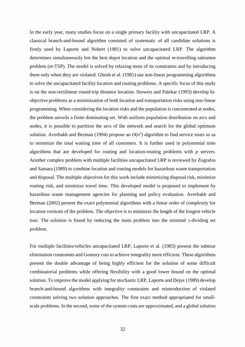
In the early year, many studies focus on a single primary facility with uncapacitated LRP. A
classical branch-and-bound algorithm consisted of systematic of all candidate solutions is
firstly used by Laporte and Nobert (1981) to solve uncapacitated LRP. The algorithm
determines simultaneously bot the best depot location and the optimal m-travelling salesmen
problem (m-TSP). The model is solved by relaxing most of its constraints and by introducing
them only when they are violated. Ghosh et al. (1981) use non-linear programming algorithms
to solve the uncapacitated facility location and routing problems. A specific focus of this study
is on the non-rectilinear round-trip distance location. Stowers and Palekar (1993) develop bi-
objective problems as a minimization of both location and transportation risks using non-linear
programming. When considering the location risks and the population is concentrated at nodes,
the problem unveils a finite dominating set. With uniform population distribution on arcs and
nodes, it is possible to partition the arcs of the network and search for the global optimum
solution. Averbakh and Berman (1994) propose an O(n2) algorithm to find service tours so as
to minimize the total waiting time of all customers. It is further used in polynomial time
algorithms that are developed for routing and location-routing problems with p servers.
Another complex problem with multiple facilities uncapacitated LRP is reviewed by Zografos
and Samara (1989) to combine location and routing models for hazardous waste transportation
and disposal. The multiple objectives for this work include minimizing disposal risk, minimize
routing risk, and minimize travel time. This developed model is proposed to implement by
hazardous waste management agencies for planning and policy evaluation. Averbakh and
Berman (2002) present the exact polynomial algorithms with a linear order of complexity for
location versions of the problem. The objective is to minimize the length of the longest vehicle
tour. The solution is found by reducing the main problem into the minimal -dividing set
problem.
For multiple facilities/vehicles uncapacitated LRP, Laporte et al. (1983) present the subtour
elimination constraints and Gomory cuts to achieve integrality more efficient. These algorithms
present the double advantage of being highly efficient for the solution of some difficult
combinatorial problems while offering flexibility with a good lower bound on the optimal
solution. To improve the model applying for stochastic LRP, Laporte and Dejax (1989) develop
branch-and-bound algorithms with integrality constraints and reintroduction of violated
constraints solving two solution approaches. The first exact method appropriated for small-
scale problems. In the second, some of the system costs are approximated, and a global solution
33
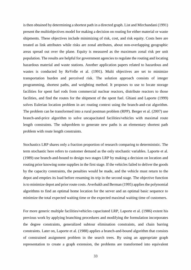
is then obtained by determining a shortest path in a directed graph. List and Mirchandani (1991)
present the multiobjectives model for making a decision on routing for either material or waste
shipments. These objectives include minimizing of risk, cost, and risk equity. Costs here are
treated as link attributes while risks are zonal attributes, about non-overlapping geographic
areas spread out over the plane. Equity is measured as the maximum zonal risk per unit
population. The results are helpful for government agencies to regulate the routing and locating
hazardous material and waste stations. Another application papers related to hazardous and
wastes is conducted by ReVelle et al. (1991). Multi objectives are set to minimize
transportation burden and perceived risk. The solution approach consists of integer
programming, shortest paths, and weighting method. It proposes to use to locate storage
facilities for spent fuel rods from commercial nuclear reactors, distribute reactors to those
facilities, and find the routes for the shipment of the spent fuel. Ghiani and Laporte (1999)
solves Eulerian location problem in arc routing context using the branch-and-cut algorithm.
The problem can be transformed into a rural postman problem (RPP). Berger et al. (2007) use
branch-and-price algorithm to solve uncapacitated facilities/vehicles with maximal route
length constraints. The subproblem to generate new paths is an elementary shortest path
problem with route length constraints.
Stochastics LRP shares only a fraction proportion of research comparing to deterministic. The
term stochastic here refers to customer demand as the only stochastic variables. Laporte et al.
(1989) use branch-and-bound to design two stages LRP by making a decision on location and
routing prior knowing some supplies in the first stage. If the vehicles failed to deliver the goods
by the capacity constraints, the penalties would be made, and the vehicle must return to the
depot and empties its load before resuming its trip in the second stage. The objective function
is to minimize depot and prior route costs. Averbakh and Berman (1995) applies the polynomial
algorithms to find an optimal home location for the server and an optimal basic sequence to
minimize the total expected waiting time or the expected maximal waiting time of customers.
For more generic multiple facilities/vehicles capacitated LRP, Laporte et al. (1986) extent his
previous work by applying branching procedures and modifying the formulation incorporates
the degree constraints, generalized subtour elimination constraints, and chain barring
constraints. Later on, Laporte et al. (1988) applies a branch-and-bound algorithm that consists
of constrained assignment problem in the search trees. By using an appropriate graph
representation to create a graph extension, the problems are transformed into equivalent
34
constrained assignment problems. Akca et al. (2009) models three exact and one heuristic
branch-and-price approaches. The subproblem uses elementary shortest path problem with
resource constraint corresponds to the labeling algorithm. Five classes of valid inequalities are
also added to the relaxed master problem to strengthen it. Base in the formulation of this study,
Baldacci et al. (2011) also describe a new exact method based on a set partitioning like the
formulation. The original problem is decomposed into a limited set of multi-capacitated depot
vehicle routing problems. It improves the quality of lower bounds and the number of the
dimensions of the instances. Belenguer et al. (2011) develop a branch-and-cut algorithm and
introduce some valid equalities. Some of them derived from capacitated vehicle routing
problem (CVRP), some of them derived from mixed-integer programming. Two new exact
polynomial algorithms are developed to separate path elimination and w-subtour elimination
constraints, and some heuristic separation procedures have been designed for all the families
of constraints. This work is extended by Contardo et al. (2013a) to compare three different flow
formulations, namely a two-index two-commodity flow formulation, a three-index vehicle-
flow formulation, and a three-index two-commodity flow formulation. The existing two-index
vehicle-flow formulation is also modified by introducing new families of valid inequalities and
separation algorithms. Contardo et al. (2013b) apply the similar approach to Akca et al. (2009)
and Baldacci et al. (2011) by using cut-and-column algorithms. The problem is solved by
column generation where the subproblem using a shortest path of minimum reduced cost under
capacity constraints. Five new families of inequalities are introduced that are shown to
dominate some of the cuts from the two-index formulation. All of these studies have solved
instances with 50 customers and 5-10 depots.
2.4 Column Generation
Column generation is the algorithm for solving the large integer of mixed integer problems.
The reason behind the issue on the large problem is that many linear programs are too large to
consider all the variables explicitly. Since most of the variables are going to be non-basic and
assume a value of zero in the optimal solution, we do not need to include all variables in the
model. Only a subset of variables needs to be included when solving the problem. The
algorithm generates only particular variables that have the potential to improve the objective
function by looking for the variables with negative reduced cost.
35
The reduced cost here is the amount of change needed in the corresponding coefficient for the
variable to enter the basis. Its sign does not necessarily give any information. At the point where
the optimal solution exists, two phenomena happen;
1. All non-basic variables have a poor reduced cost since they cannot produce a better
solution.
2. All basic variables have a zero negative cost since they are already in the basis.
For general problem P, the regular form to model a column generation is;
Pp
Ppxcmin (2.21)
subject to
Pp
pp bxa (2.22)
0px Pp (2.23)
In each iteration, it looks for a non-basic variable to price out and enter the basis. In the
subproblem, given the vector 0 as dual variables, the cost is replaced as;
pT
pp acc , Pp (2.24)
An explicit search of P may be computationally impossible when |P| is huge. Therefore, it is
more practical to determine only a subset P’ P of columns, with restricted master problem
(RMP).
The purpose of RMP is to determine the dual variables, transfer to the subproblem, and control
the stopping criterion. Primal methods maintain primal feasibility and work towards dual
feasibility. It is therefore only natural to monitor the dual solution in the course of the algorithm.
A dual solution to the RMP needs not be unique, e.g., if the primal is degenerate. It is significant
in as much the dual solution directly influences the selection of new columns. Because a dual
basic solution corresponds to an extreme point of the optimal face, it may be a bad
representative of all the dual solutions obtainable (Lübbecke & Desrosiers, 2005).
The application of column generation in VRP and LRP is described in Chapter 3 of this
dissertation. More details on the survey papers of column generation can be found in Barnhart
et al. (1998), Wilhelm (2001), Lübbecke & Desrosiers (2005), and Desaulniers et al. (2005).
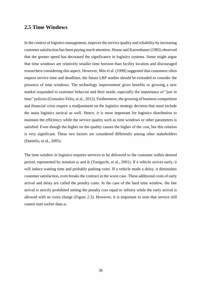
36
2.5 Time Windows
In the context of logistics management, improve the service quality and reliability by increasing
customer satisfaction has been paying much attention. House and Karrenbauer (1982) observed
that the greater speed has decreased the significance in logistics systems. Some might argue
that time windows are relatively smaller time horizon than facility location and discouraged
researchers considering this aspect. However, Min et al. (1998) suggested that customers often
request service time and deadlines, the future LRP studies should be extended to consider the
presence of time windows. The technology improvement gives benefits to growing a new
market responded to customer behavior and their needs, especially the importance of “just in
time” policies (Gonzalez-Feliu, et al., 2012). Furthermore, the growing of business competition
and financial crisis require a readjustment on the logistics strategy decision that must include
the main logistics tactical as well. Hence, it is most important for logistics distribution to
maintain the efficiency while the service quality such as time windows or other parameters is
satisfied. Even though the higher on the quality causes the higher of the cost, but this relation
is very significant. These two factors are considered differently among other stakeholders
(Danielis, et al., 2005).
The time window in logistics requires services to be delivered to the customer within desired
period, represented by notation ai and bi (Taniguchi, et al., 2001). If a vehicle arrives early, it
will induce waiting time and probably parking costs. If a vehicle made a delay, it diminishes
customer satisfaction, even breaks the contract in the worst case. These additional costs of early
arrival and delay are called the penalty costs. In the case of the hard time window, the late
arrival is strictly prohibited setting the penalty cost equal to infinity while the early arrival is
allowed with no extra charge (Figure 2.3). However, it is important to note that service still
cannot start earlier than ai.
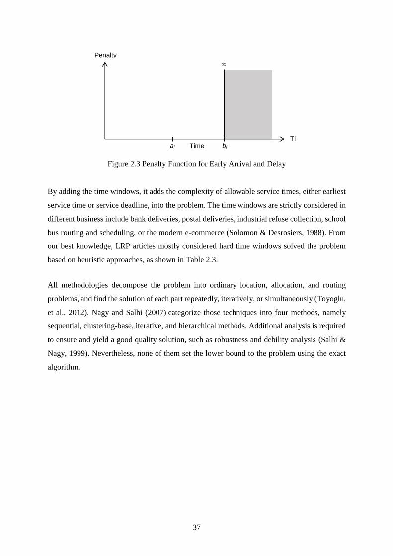
37
Figure 2.3 Penalty Function for Early Arrival and Delay
By adding the time windows, it adds the complexity of allowable service times, either earliest
service time or service deadline, into the problem. The time windows are strictly considered in
different business include bank deliveries, postal deliveries, industrial refuse collection, school
bus routing and scheduling, or the modern e-commerce (Solomon & Desrosiers, 1988). From
our best knowledge, LRP articles mostly considered hard time windows solved the problem
based on heuristic approaches, as shown in Table 2.3.
All methodologies decompose the problem into ordinary location, allocation, and routing
problems, and find the solution of each part repeatedly, iteratively, or simultaneously (Toyoglu,
et al., 2012). Nagy and Salhi (2007) categorize those techniques into four methods, namely
sequential, clustering-base, iterative, and hierarchical methods. Additional analysis is required
to ensure and yield a good quality solution, such as robustness and debility analysis (Salhi &
Nagy, 1999). Nevertheless, none of them set the lower bound to the problem using the exact
algorithm.
Penalty Cost
Timai bi
Time window
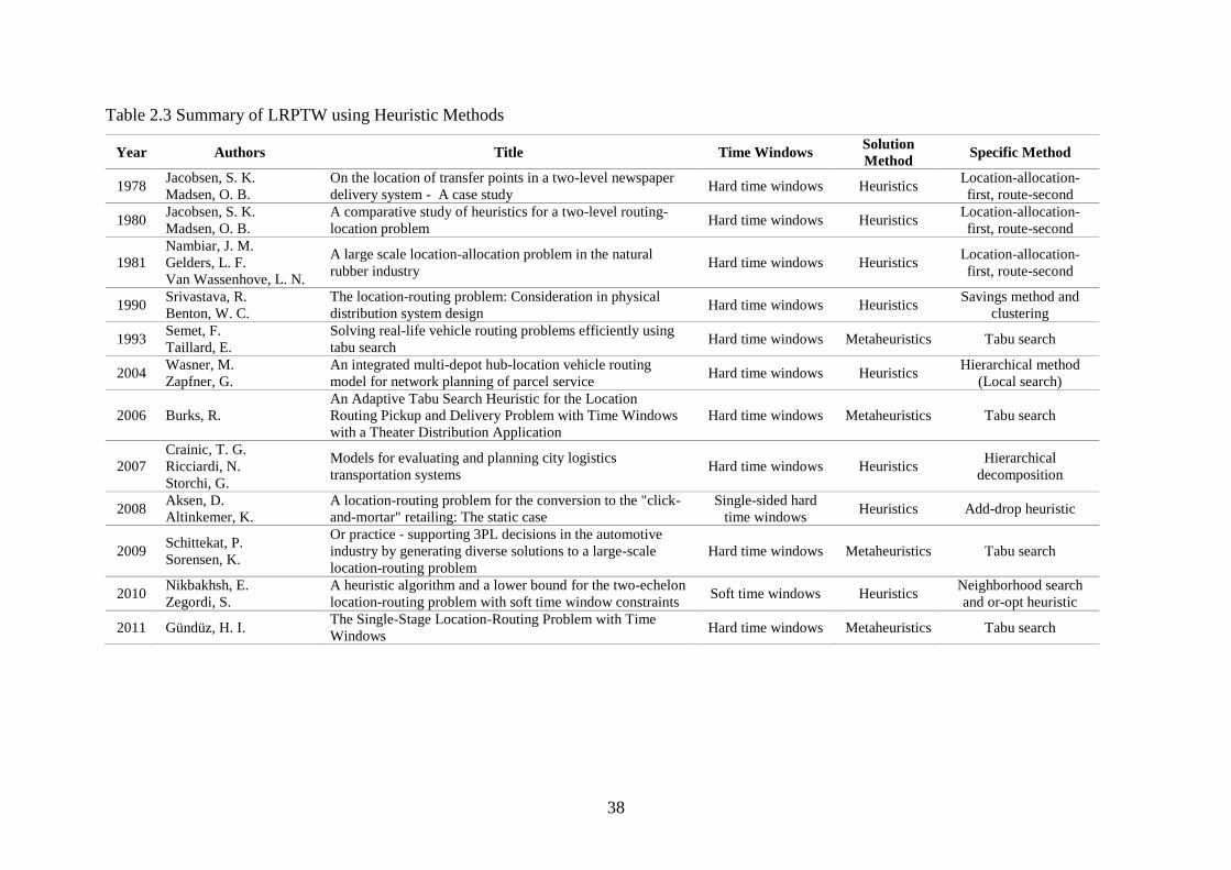
38
Table 2.3 Summary of LRPTW using Heuristic Methods
Year Authors Title Time Windows Solution
Method Specific Method
1978 Jacobsen, S. K.
Madsen, O. B.
On the location of transfer points in a two-level newspaper
delivery system - A case study Hard time windows Heuristics
Location-allocation-
first, route-second
1980 Jacobsen, S. K.
Madsen, O. B.
A comparative study of heuristics for a two-level routing-
location problem Hard time windows Heuristics
Location-allocation-
first, route-second
1981
Nambiar, J. M.
Gelders, L. F.
Van Wassenhove, L. N.
A large scale location-allocation problem in the natural
rubber industry Hard time windows Heuristics
Location-allocation-
first, route-second
1990 Srivastava, R.
Benton, W. C.
The location-routing problem: Consideration in physical
distribution system design Hard time windows Heuristics
Savings method and
clustering
1993 Semet, F.
Taillard, E.
Solving real-life vehicle routing problems efficiently using
tabu search Hard time windows Metaheuristics Tabu search
2004 Wasner, M.
Zapfner, G.
An integrated multi-depot hub-location vehicle routing
model for network planning of parcel service Hard time windows Heuristics
Hierarchical method
(Local search)
2006 Burks, R.
An Adaptive Tabu Search Heuristic for the Location
Routing Pickup and Delivery Problem with Time Windows
with a Theater Distribution Application
Hard time windows Metaheuristics Tabu search
2007
Crainic, T. G.
Ricciardi, N.
Storchi, G.
Models for evaluating and planning city logistics
transportation systems Hard time windows Heuristics
Hierarchical
decomposition
2008 Aksen, D.
Altinkemer, K.
A location-routing problem for the conversion to the "click-
and-mortar" retailing: The static case
Single-sided hard
time windows Heuristics Add-drop heuristic
2009 Schittekat, P.
Sorensen, K.
Or practice - supporting 3PL decisions in the automotive
industry by generating diverse solutions to a large-scale
location-routing problem
Hard time windows Metaheuristics Tabu search
2010 Nikbakhsh, E.
Zegordi, S.
A heuristic algorithm and a lower bound for the two-echelon
location-routing problem with soft time window constraints Soft time windows Heuristics
Neighborhood search
and or-opt heuristic
2011 Gündüz, H. I. The Single-Stage Location-Routing Problem with Time
Windows Hard time windows Metaheuristics Tabu search
39
2.6 Benchmark Instances
Unlike other routing and scheduling problems, the benchmarks or instances for LRPTW have
not been generated and shared by other researchers publicly. The existing well-known VRPTW
benchmark developed by Solomon (1987) is used in this study. It consists of three main
categories, R-Type (random), C-Type (clustered), and RC-Type (mixed random/clustered)
(Figure 2.4). Each category is designed to several factors that affect the behavior of routing and
scheduling algorithms, including
Geographical data
Number of customers serviced by a vehicle
Percent of time-constrained customers
Tightness and positioning of the time windows
The largest problems are 100 customer problems where travel times equal the corresponding
Euclidean distances. In each category, the customer coordinates are identical for all problems
within one type. The problems differ with respect to the width of the time windows. Some have
very tight time windows while others have time windows that are hardly constraining. In terms
of time window density or the percentage of customers with time windows, they are created
with 25, 50, 75 and 100% time windows. Also, the problem sets R1, C1 and RC1 have a short
scheduling horizon and allow only a few customers per route (approximately 5 to 10). In
contrast, the sets R2, C2 and RC2 have a long scheduling horizon permitting many customers
(more than 30) to be served by the same vehicle. For each such problem, smaller problems
have been created by considering only the first 25 or 50 customers. Figure 2.5 shows the details
of the small problem of R101 with 25 customers. The label of each customer represents
customer number, demand, and time windows [a,b].

40
Figure 2.4 Locations of Depot and Customers in R (top), C (middle), and RC (below)
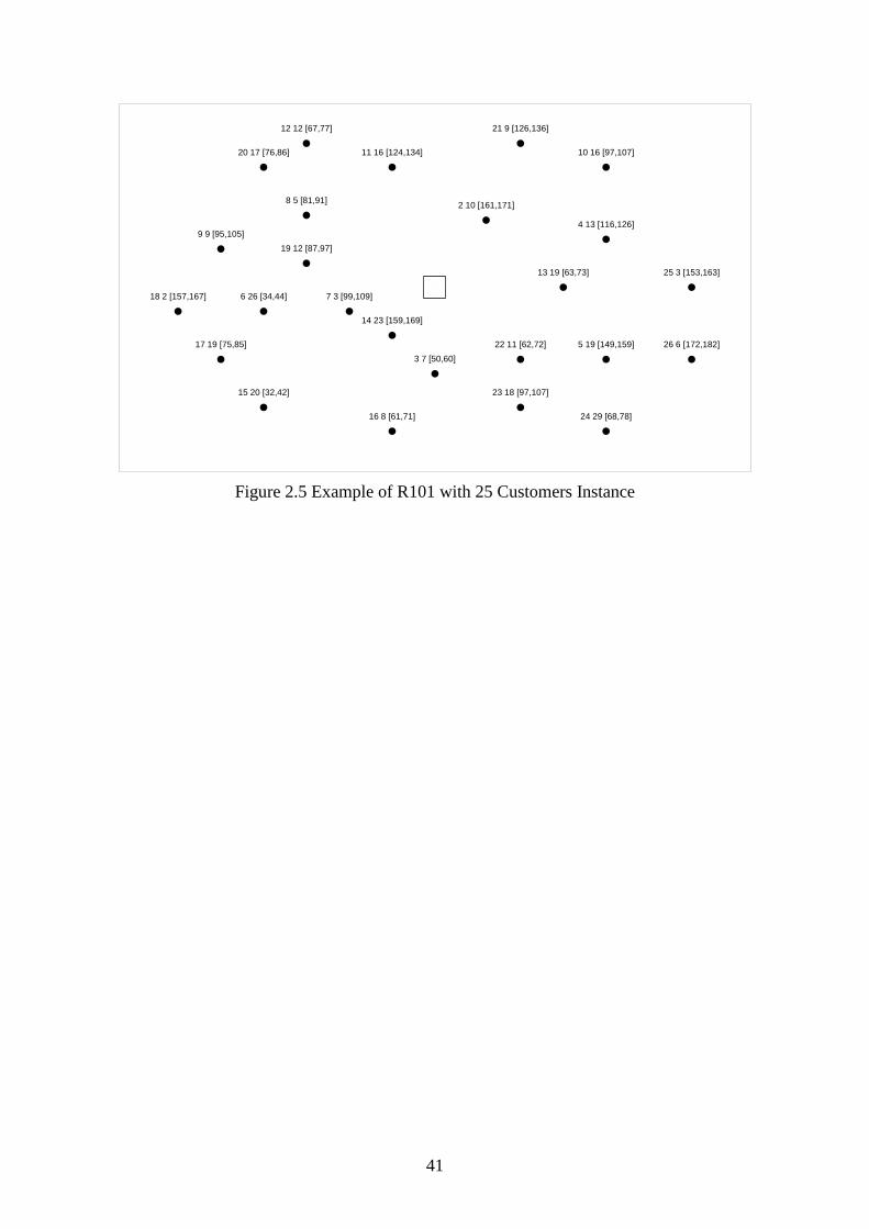
41
Figure 2.5 Example of R101 with 25 Customers Instance
2 10 [161,171]
3 7 [50,60]
4 13 [116,126]
5 19 [149,159]
6 26 [34,44] 7 3 [99,109]
8 5 [81,91]
9 9 [95,105]
10 16 [97,107]11 16 [124,134]
12 12 [67,77]
13 19 [63,73]
14 23 [159,169]
15 20 [32,42]
16 8 [61,71]
17 19 [75,85]
18 2 [157,167]
19 12 [87,97]
20 17 [76,86]
21 9 [126,136]
22 11 [62,72]
23 18 [97,107]
24 29 [68,78]
25 3 [153,163]
26 6 [172,182]
D1
42
References
Akca, Z., Berger, R. & Ralphs, T., 2009. A branch-and-price algorithm for combined location
and routing problems under capacity restrictions. In: J. W. Chinneck, B. Kristjansson &
M. J. Saltzman, eds. Operations Research and Cyber-Infrastructure. s.l.:Springer US, pp.
309-330.
Aksen, D. & Altinkemer, K., 2008. A location-routing problem for the conversion to the
"click-and-mortar" retailing: The static case. European Journal of Operational Research,
Volume 186(2), pp. 554-575.
Averbakh, I. & Berman, O., 1994. Routing and location-routing p-delivery men problems on
a path. Transportation Science, Volume 28, p. 162–166.
Averbakh, I. & Berman, O., 1995. Probabilistic sales-delivery man and sales-delivery facility
location problems on a tree. Transportation Science, 29(2), pp. 184-197.
Averbakh, I. & Berman, O., 2002. Minmax p-traveling salesmen location problems on a tree.
Annals of Operations Research, Volume 110, pp. 55-68.
Baldacci, R., Mingozzi, A. & Wolfler Calvo, R., 2011. An exact method for the capacitated
location-routing problem. Operations Research, 59(5), pp. 1284-1296.
Barnhart, C. et al., 1998. Branch-and-price: Column generation for solving huge integer
programs. Operations Research, 46(3), pp. 316-329.
Belengure, J., Benavent, E. & Prins, C., 2011. A branch-and-cut method for the capacitated
location-routing problem. Computers & Operations Research, Volume 38, pp. 931-941.
Berger, R. T., Coullard, C. R. & Daskin, M. S., 2007. Location-routing problems with
distance constraints. Transportation Science, 41(1), pp. 29-43.
Berman, O., Jaillet, P. & Simchi-Levi, D., 1995. Location-routing problems with uncertainty.
In: Z. Drezner, ed. Facility Location: A Survey of Applications and Methods. New York:
Springer, p. 427–452.
Burks, R., 2006. An adaptive tabu search heuristic for the location routing pickup and
delivery problem with time windows with a theater distribution application, Ohio:
Dissertation, Air Force Institute of Technology.
Church, R. L. & ReVelle, C. S., 1976. Theoretical and computational links between the p-
median location set-covering and the maximal covering location problem. Geographical
Analysis, Volume 8, p. 406–415.
43
Church, R. & ReVelle, C., 1974. The maximal covering location problem. Regional Science
Association Papers, Volume 32, p. 101–118.
Contardo, C., Cordeau, J. F. & Gendron, B., 2013a. A computational comparison of flow
formulations for the capacitated location-routing problem. Discrete Optimization, 10(4),
pp. 263-295.
Contardo, C., Cordeau, J. F. & Gendron, B., 2013b. An exact algorithm based on cut-and-
column generation for the capacitated location-routing problem. INFORMS Journal on
Computing, 26(1), pp. 88-102.
Crainic, T. G., Ricciardi, N. & Storchi, G., 2007. Models for evaluating and planning city
logistics transportation systems, Montréal: CIRRELT.
Danielis, R., Marcucci, E. & Rotaris, L., 2005. Logistics managers’ stated preferences for
freight service attributes. Transportation Research Part E, Volume 41, pp. 201-215.
Daskin, M. S., 2013. Network and Discrete Location: Models, Algorithms, and Applications.
2 ed. s.l.:John Wiley & Sons.
Desaulniers, G., Desrosiers, J. & Solomon, M. M., 2005. Column generation. New York:
Springer Science & Business Media.
Drexl, M. & Schneider, M., 2013. A survey of location-routing problems, Mainz: Johannes
Gutenberg University.
Eilon, S., Watson-Gandy, C. D. T. & Christofides, N., 1971. Distribution Management:
Mathematical Modeling and Practical Analysis. London: Griffin.
Friedric, C. J., 1929. Alfred Weber's Theory of the Location of Industries. Chicago:
University of Chicago Press.
Galvão, R., 1993. The use of Lagrangean relaxation in the solution of uncapacitated facility
location problems. Location Science, Volume 1, p. 57–79.
Ghiani, G. & Larporte, G., 1999. Eulerian Location Problems. Networks, Volume 34, pp.
291-302.
Ghosh, J. K., Sinha, S. B. & Acharya, D., 1981. A generalized reduced gradient based
approach to round-trip location problem. In: N. K. Jaiswal, ed. Scientific Management of
Transport Systems. Amsterdam: North-Holland, pp. 209-213.
Goetschalckx, M., 2011. Supply chain engineering. 8 ed. s.l.:Springer Science & Business
Media.
Gonzalez-Feliu, J., Ambrosini, C. & Routhier, J. L., 2012. New trends on urban goods
movement: Modelling and simulation of e-commerce distribution. European Transport,
Volume 50, p. 23.
44
Gündüz, H. I., 2011. The Single-Stage Location-Routing Problem with Time Windows. In: J.
W. Böse, et al. eds. Computational Logistics. Hamburg: Springer Berlin Heidelberg, pp.
44-58.
Hakimi, S. L., 1964. Optimum locations of switching centers and the absolute centers and
medians of a graph. Operations Research, Volume 12, p. 450–459.
Hakimi, S. L., 1965. Optimal distribution of switching centers in a communication network
and some related theoretic graph theoretic problems. Operations Research, Volume 13, p.
462–475.
Hansen, P. & Thisse, J. F., 1983. Recent advances in continuous location theory. Sistemi
Urbani, Volume 1, p. 33–54.
Harrison, H., 1979. A planning system for facilities and resources in distribution networks.
Interfaces, 9(2), pp. 6-22.
Hassanzadeh, A. et al., 2009. Location-Routing Problem. s.l.:Springer.
Jacobsen, S. K. & Madsen, O. B., 1978. On the location of transfer points in a two-level
newspaper delivery system - A case study. Banff, Alberta, Canada, The International
Symposium on Location Decisions, pp. 24-28.
Jacobsen, S. K. & Madsen, O. B., 1980. A comparative study of heuristics for a two-level
routing-location problem. European Journal of Operational Research, 5(6), pp. 378-387.
Kariv, O. & Hakimi, S. L., 1979. An algorithmic approach to network location problems. Part
II: The p-median. SIAM Journal of Applied Mathematics, Volume 37, p. 539–560.
Klose, A. & Drexl, A., 2005. Facility location models for distribution system design.
European Journal of Operational Research, 162(1), p. 4–29.
Kuehn, A. A. & Hamburger, M. J., 1963. A heuristic program for locating warehouses.
Management Science, Volume 9, p. 643–666.
Laporte, G. & Dejax, P. J., 1989. Dynamic location-routeing problems. Journal of the
Operational Research Society, 40(5), pp. 471-482.
Laporte, G., Louveaux, F. & Mercure, H., 1989. Models and exact solutions for a class of
stochastic location-routing problems. European Journal of Operational Research, 39(1),
pp. 71-78.
Laporte, G. & Nobert, Y., 1981. An exact algorithm for minimizing routing and operating
costs in depot location. European Journal of Operational Research, 6(2), pp. 224-226.
Laporte, G., Nobert, Y. & Arpin, D., 1986. An exact algorithm for solving a capacitated
location-routing problem. Annals of Operations Research, Volume 6, pp. 293-310.
45
Laporte, G., Nobert, Y. & Pelletier, P., 1983. Hamiltonian Location Problems. European
Journal of Operational Research, Volume 12, pp. 82 - 89.
Laporte, G., Nobert, Y. & Taillefer, S., 1988. Solving a family of multi-depot vehicle routing
and location-routing problems. Transportation science, 22(3), pp. 161-172.
Larporte, G. & Nobert, Y., 1981. An exact algorithm for minimizing routing and operating
costs in depot location. European Journal of Operational Research, 6(2), pp. 224-226.
List, G. & Mirchandani, P., 1991. An integrated network/planar multiobjective model for
routing and siting for hazardous materials and wastes. Transportation Science, 25(2), pp.
146-156.
Lübbecke, M. E. & Desrosiers, J., 2005. Selected topics in column generation. Operations
Research, 53(6), pp. 1007-1023.
Madsen, O. B., 1983. Methods for solving combined two level location-routing problems of
realistic dimensions. European Journal of Operational Research, 12(3), pp. 295-301.
Maranzana, F., 1964. On the location of supply points to minimize transport costs.
Operations Research Quarterly, Volume 15, p. 261–270.
Min, H., Jayaraman, V. & Srivastara, R., 1998. Combined location-routing problem: A
synthesis and future research directions. European Journal of Operational Research,
108(1), pp. 1-15.
Nagy, G. & Salhi, S., 2007. Location-routing: Issues, models and methods. European Journal
of Operational Research, 177(2), p. 649–672.
Nambiar, J. M., Gelders, L. F. & Van Wassenhove, L. N., 1981. A large scale location-
allocation problem in the natural rubber industry. European Journal of Operational
Research, 6(2), pp. 183-189.
Nikbakhsh, E. & Zegordi, S., 2010. A heuristic algorithm and a lower bound for the two-
echelon location-routing problem with soft time window constraints. Scientia Iranica
Transaction E: Industrial Engineering, Volume 17(1), pp. 36-47.
Or, I. & Pierskalla, W. P., 1979. A Transportation Location-Allocation Model for Regional
Blood Banking. AIIE transactions, 11(2), pp. 86-95.
Prodhon, C., 2011. A hybrid evolutionary algorithm for periodic location-routing problem.
European Journal of Operational Research, Volume 210, pp. 204-212.
Prodhon, C. & Prins, C., 2014. A survey of recent research on location-routing problems.
European Journal of Operational Research, 238(1), pp. 1-17.
Rand, G. K., 1976. Methodological choices in depot location studies. Operational Research
Quarterly, Volume 27, p. 241–249.
46
ReVelle, C., Cohon, J. & Shobrys, D., 1991. Simultaneous siting and routing in the disposal
of hazardous wastes. Transportation Science, 25(2), pp. 138-145.
ReVelle, C. S. & Swain, R. W., 1970. Central facilities location. Geographical Analysis,
Volume 2, p. 30–42.
Rosing, K. & ReVelle, C., 1997. Heuristic concentration: Two stage solution construction.
European Journal of Operational Research, Volume 97, p. 75–86.
Salhi, S. & Nagy, G., 1999. Consistency and Robustness in Location-Routing. Studies in
Locational Analysis, pp. 3-19.
Salhi, S. & Rand, G., 1989. The Effect of Ignoring Routes when Locating Depots. European
Journal of Operation Research, 39(2), pp. 150-156.
Schilling, D., Rosing, K. & ReVelle, C., 2000. Network distance characteristics that affect
computational effort in the p-median problem. European Journal of Operational
Research, Volume 127, p. 525–536.
Schittekat, P. & Sorensen, K., 2009. Or practice - supporting 3PL decisions in the automotive
industry by generating diverse solutions to a large-scale location-routing problem.
Operations Research, Volume 57(5), pp. 1058-1067.
Semet, F. & Taillard, E., 1993. Solving real-life vehicle routing problems efficiently using
tabu search. Annals of Operations Research, Volume 41, p. 469–488.
Solomon, M. M., 1987. Algorithms for the vehicle routing and scheduling problems with
time window constraints. Operations research, 35(2), pp. 254-265.
Solomon, M. M. & Desrosiers, J., 1988. Survey Paper - Time Window Constrained Routing
and Scheduling Problems. Transportation Science, Volume 22(1), pp. 1-13.
Srivastava, R. & Benton, W. C., 1990. The location-routing problem: Consideration in
physical distribution system design. Computers and Operations Research, Volume 6, pp.
427-435.
Stowers, C. L. & Palekar, U. S., 1993. Location models with routing considerations for a
single obnoxious facility. Transportation Science, Volume 27, p. 350–362.
Taniguchi, E., Thompson, R. G., Yamada, T. & Duin, R. V., 2001. City Logistics. Oxford:
Elsevier Science Ltd..
Teitz, M. & Bart, P., 1968. Heuristic methods for estimating the generalized vertex median of
a weighted graph. Operations Research, Volume 16, p. 955–961.
Tellier, L. N., 1972. The Webber Problem: Solution and Interpretation*. Geographical
Analysis, 4(3), pp. 215-233.
47
Toregas, C., Swain, R., ReVelle, C. & Bergmann, L., 1971. The location of emergency
service facilities. Operations Research, Volume 19, p. 1363–1373.
Toyoglu, H., Karasan, O. & Kara, B., 2012. A New Formulation Approach for Location-
Routing Problems. Networks and Spatial Economics, Volume 12, pp. 635-659.
Wasner, M. & Zapfner, G., 2004. An integrated multi-depot hub-location vehicle routing
medel for network planning of parcel service. Operations Research Letters, Volume 20,
pp. 403-419.
Watson-Gandy, C. D. T. & Dohrn, P. J., 1973. Depot location with van salesmen - a practical
approach. Omega, 1(3), pp. 321-329.
Wilhelm, W. E., 2001. A technical review of column generation in integer programming.
Optimization and Engineering, 2(2), pp. 159-200.
Zografos, K. G. & Samara, S., 1989. Combined location-routing model for hazardous waste
transportation and disposal. Transportation Research Record, Volume 1245, p. 52–59.

48
49
Chapter 3
Methodology
3.1 Formulation
3.2 Branch-and-Price Algorithm
3.2.1 The Master Problem
3.2.2 The Subproblem (Pricing Problem)
3.2.3 Accelerating Processes
3.2.4 Branching Strategies
3.3 Example of Branch-and-Price algorithm for LRPTW
References

50
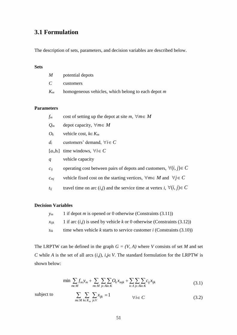
51
3.1 Formulation
The description of sets, parameters, and decision variables are described below.
Sets
M potential depots
C customers
Km homogeneous vehicles, which belong to each depot m
Parameters
fm cost of setting up the depot at site m, Mm
Qm depot capacity, Mm
Ok vehicle cost, kKm
di customers’ demand, Ci
[ai,bi] time windows, Ci
q vehicle capacity
cij operating cost between pairs of depots and customers, Cji ),(
cmj vehicle fixed cost on the starting vertices, Mm and Cj
tij travel time on arc (i,j) and the service time at vertex i, Cji ),(
Decision Variables
ym 1 if depot m is opened or 0 otherwise (Constraints (3.11))
xijk 1 if arc (i,j) is used by vehicle k or 0 otherwise (Constraints (3.12))
sik time when vehicle k starts to service customer i (Constraints (3.10))
The LRPTW can be defined in the graph G = (V, A) where V consists of set M and set
C while A is the set of all arcs (i,j), i,jV. The standard formulation for the LRPTW is
shown below:
Ai Aj Kk
ijkijMm Aj Kk
mjkkMm
mm xcxOyfmin (3.1)
subject to 1 Mm Kk Vj
ijk
m
x Ci (3.2)
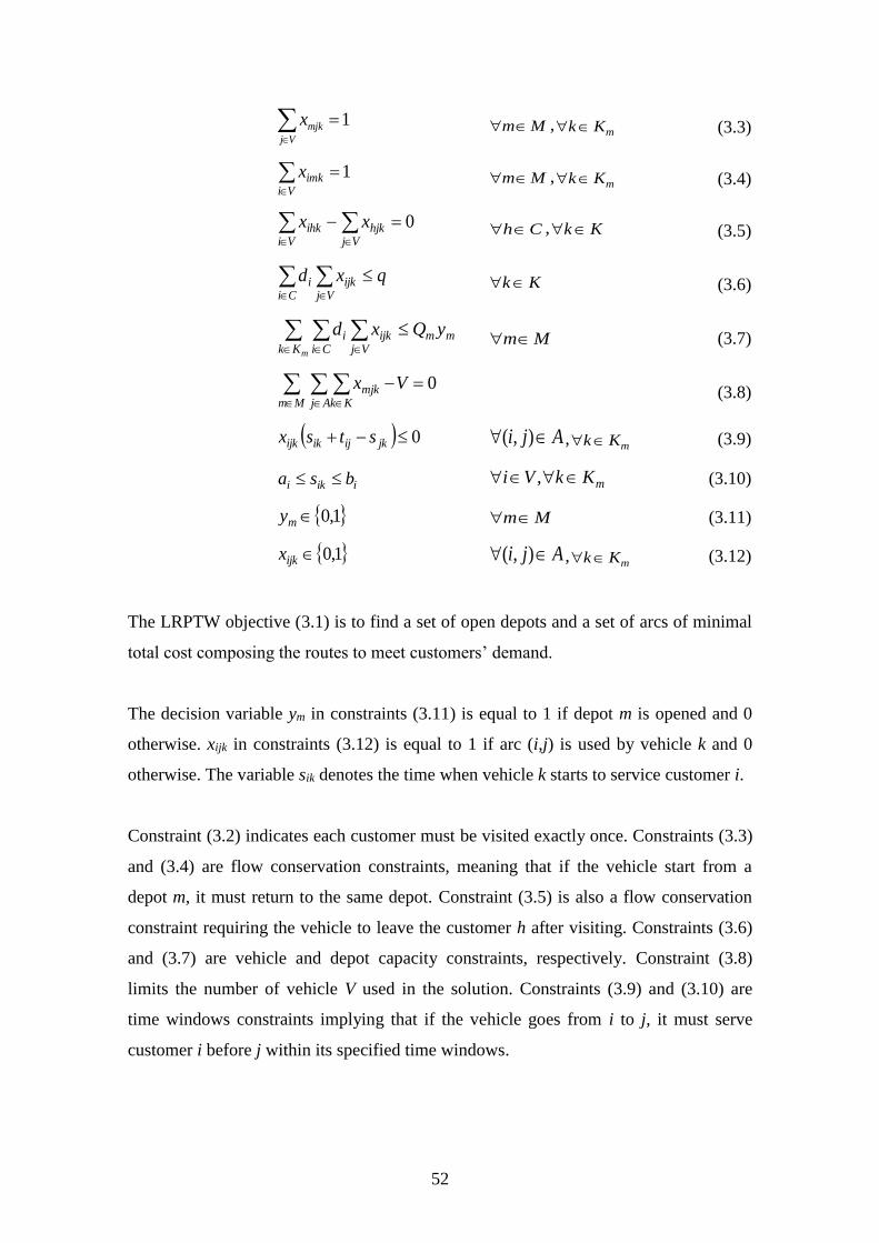
52
1Vj
mjkx Mm ,mKk (3.3)
1Vi
imkx Mm ,mKk (3.4)
0 Vj
hjkVi
ihk xx Ch , Kk (3.5)
qxdCi Vj
ijki
Kk (3.6)
mKkmm
Ci Vjijki yQxd
Mm (3.7)
0
VxMm Aj Kk
mjk (3.8)
0 jkijikijk stsx Aji ),( ,mKk (3.9)
iiki bsa mKkVi , (3.10)
1,0my Mm (3.11)
1,0ijkx Aji ),( ,mKk (3.12)
The LRPTW objective (3.1) is to find a set of open depots and a set of arcs of minimal
total cost composing the routes to meet customers’ demand.
The decision variable ym in constraints (3.11) is equal to 1 if depot m is opened and 0
otherwise. xijk in constraints (3.12) is equal to 1 if arc (i,j) is used by vehicle k and 0
otherwise. The variable sik denotes the time when vehicle k starts to service customer i.
Constraint (3.2) indicates each customer must be visited exactly once. Constraints (3.3)
and (3.4) are flow conservation constraints, meaning that if the vehicle start from a
depot m, it must return to the same depot. Constraint (3.5) is also a flow conservation
constraint requiring the vehicle to leave the customer h after visiting. Constraints (3.6)
and (3.7) are vehicle and depot capacity constraints, respectively. Constraint (3.8)
limits the number of vehicle V used in the solution. Constraints (3.9) and (3.10) are
time windows constraints implying that if the vehicle goes from i to j, it must serve
customer i before j within its specified time windows.
53
3.2 Branch-and-Price Algorithm
The branch-and-price algorithm is the embedded algorithm between column generation
techniques within a linear programming based and branch-and-bound framework
(Lübbecke & Desrosiers, 2005). It is first introduced by Desrosiers et al. (1984) for
solving the vehicle routing problem with time windows. Column generation follows the
idea of the Dantzig-Wolfe decomposition (Dantzig & Wolfe, 1960) by splitting original
formulation into two problems: the master and the subproblems. The master problem
considers only a subset of variables from the original while the subproblem identifies
the new variables. The objective function of the subproblem considers the reduced cost
of the new variables with respect to the current dual variables. The outline of branch-
and-price algorithm is illustrated in Figure 3.1.
The process works as follows: the master problem is solved using an initial solution. It
can be any feasible solution that meets all constraints (Perrot, 2005). In this case, we
start with the depot-i-depot routes. From this step, the dual prices of each constraint in
the master problem are obtained. Then, the reduced cost is calculated and utilized in the
objective function of the subproblem. After solving the subproblem, the variables
called columns in the master problem with negative reduced cost must be identified.
Then, these variables are added to the master problem and resolved iteratively. The
process is repeated until the subproblem solution has only non-negative reduced costs
columns. Theoretically, at that instance, the solution of the master problem is the
optimal solution.
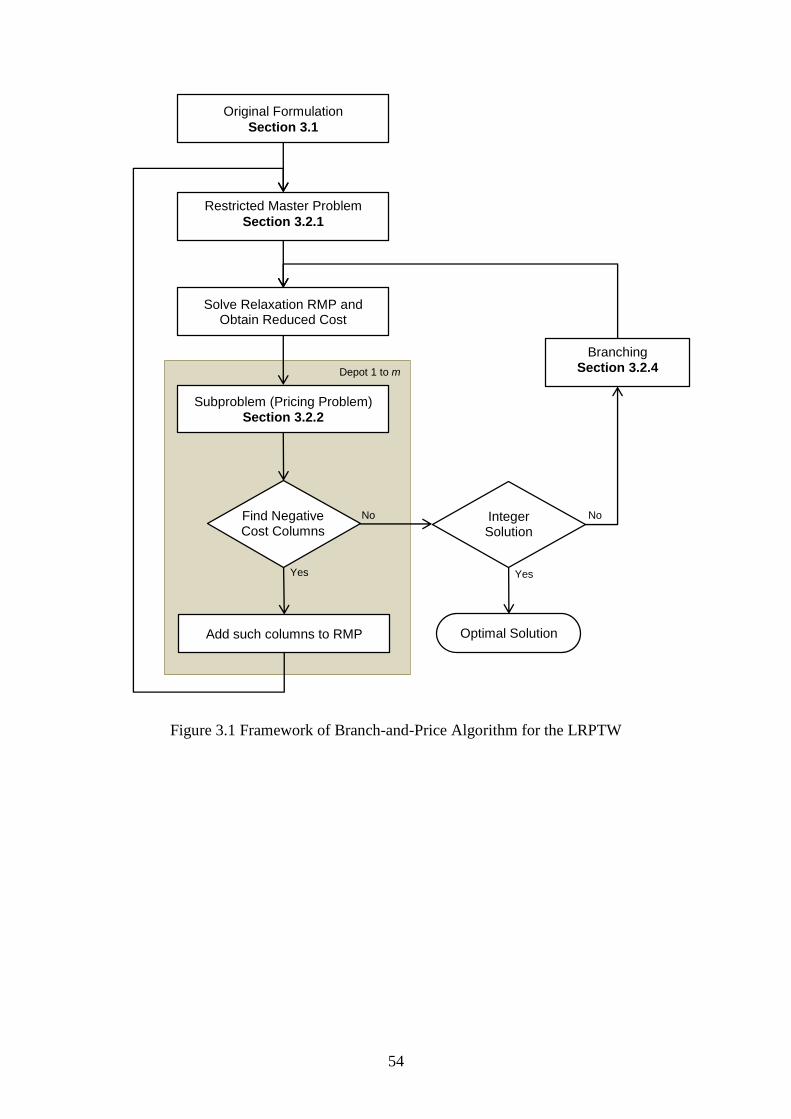
54
Figure 3.1 Framework of Branch-and-Price Algorithm for the LRPTW
Depot 1 to m
Original Formulation
Section 3.1
Restricted Master Problem
Section 3.2.1
Solve Relaxation RMP and Obtain Reduced Cost
Subproblem (Pricing Problem) Section 3.2.2
Integer Solution
Add such columns to RMP Optimal Solution
Branching Section 3.2.4
Yes Yes
No No Find Negative Cost Columns
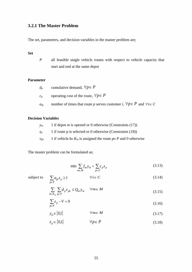
55
3.2.1 The Master Problem
The set, parameters, and decision variables in the master problem are;
Set
P all feasible single vehicle routes with respect to vehicle capacity that
start and end at the same depot
Parameter
dp cumulative demand, Pp
cp operating cost of the route, Pp
aip number of times that route p serves customer i, Pp and Ci
Decision Variables
ym 1 if depot m is opened or 0 otherwise (Constraints (17))
zp 1 if route p is selected or 0 otherwise (Constraints (18))
vpk 1 if vehicle kKm is assigned the route pP and 0 otherwise
The master problem can be formulated as;
Pp
ppMm
mm zcyfmin (3.13)
subject to
Pp
pip za 1 Ci (3.14)
mKkmm
Pppkp yQvd Mm
(3.15)
Pp
p Vz 0 (3.16)
1,0my Mm (3.17)
1,0pz Pp (3.18)
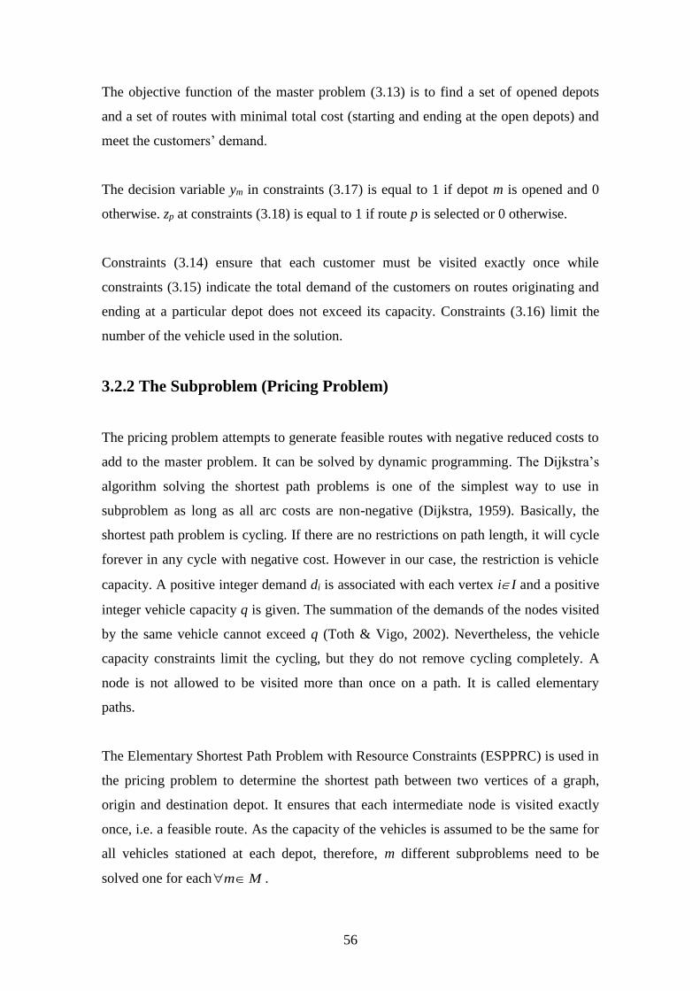
56
The objective function of the master problem (3.13) is to find a set of opened depots
and a set of routes with minimal total cost (starting and ending at the open depots) and
meet the customers’ demand.
The decision variable ym in constraints (3.17) is equal to 1 if depot m is opened and 0
otherwise. zp at constraints (3.18) is equal to 1 if route p is selected or 0 otherwise.
Constraints (3.14) ensure that each customer must be visited exactly once while
constraints (3.15) indicate the total demand of the customers on routes originating and
ending at a particular depot does not exceed its capacity. Constraints (3.16) limit the
number of the vehicle used in the solution.
3.2.2 The Subproblem (Pricing Problem)
The pricing problem attempts to generate feasible routes with negative reduced costs to
add to the master problem. It can be solved by dynamic programming. The Dijkstra’s
algorithm solving the shortest path problems is one of the simplest way to use in
subproblem as long as all arc costs are non-negative (Dijkstra, 1959). Basically, the
shortest path problem is cycling. If there are no restrictions on path length, it will cycle
forever in any cycle with negative cost. However in our case, the restriction is vehicle
capacity. A positive integer demand di is associated with each vertex iI and a positive
integer vehicle capacity q is given. The summation of the demands of the nodes visited
by the same vehicle cannot exceed q (Toth & Vigo, 2002). Nevertheless, the vehicle
capacity constraints limit the cycling, but they do not remove cycling completely. A
node is not allowed to be visited more than once on a path. It is called elementary
paths.
The Elementary Shortest Path Problem with Resource Constraints (ESPPRC) is used in
the pricing problem to determine the shortest path between two vertices of a graph,
origin and destination depot. It ensures that each intermediate node is visited exactly
once, i.e. a feasible route. As the capacity of the vehicles is assumed to be the same for
all vehicles stationed at each depot, therefore, m different subproblems need to be
solved one for each Mm .
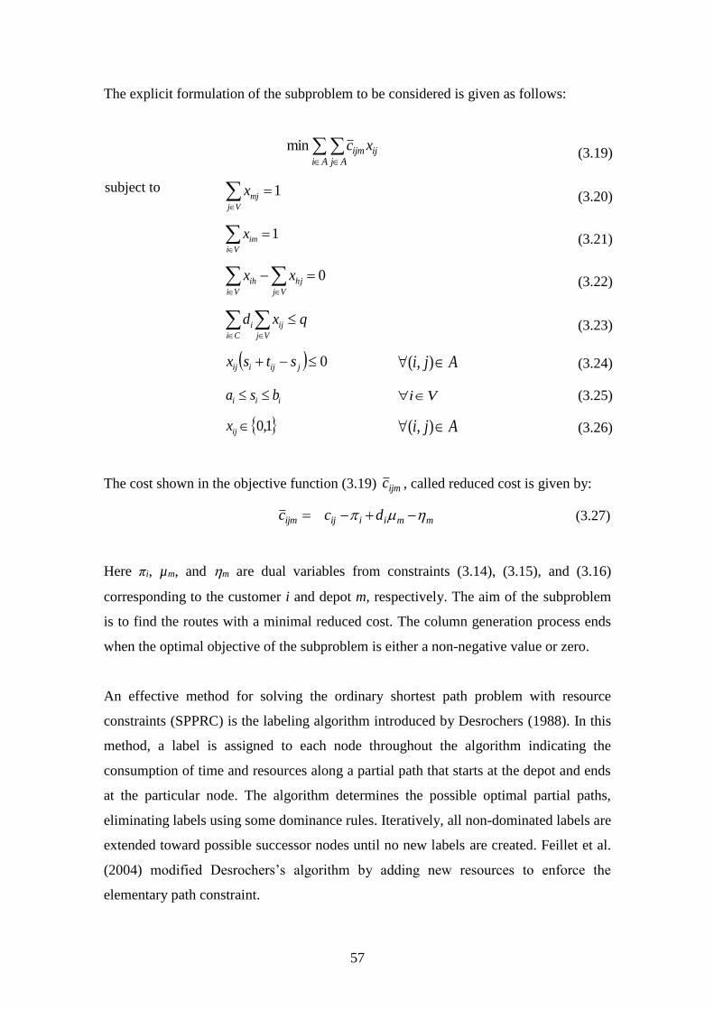
57
The explicit formulation of the subproblem to be considered is given as follows:
Ai Aj
ijijm xcmin (3.19)
subject to 1Vj
mjx (3.20)
1Vi
imx (3.21)
0 Vj
hj
Vi
ih xx (3.22)
qxdCi Vj
iji
(3.23)
0 jijiij stsx Aji ),( (3.24)
iii bsa Vi (3.25)
1,0ijx Aji ),( (3.26)
The cost shown in the objective function (3.19) ijmc , called reduced cost is given by:
mmiiijijm dcc (3.27)
Here πi, µm, and m are dual variables from constraints (3.14), (3.15), and (3.16)
corresponding to the customer i and depot m, respectively. The aim of the subproblem
is to find the routes with a minimal reduced cost. The column generation process ends
when the optimal objective of the subproblem is either a non-negative value or zero.
An effective method for solving the ordinary shortest path problem with resource
constraints (SPPRC) is the labeling algorithm introduced by Desrochers (1988). In this
method, a label is assigned to each node throughout the algorithm indicating the
consumption of time and resources along a partial path that starts at the depot and ends
at the particular node. The algorithm determines the possible optimal partial paths,
eliminating labels using some dominance rules. Iteratively, all non-dominated labels are
extended toward possible successor nodes until no new labels are created. Feillet et al.
(2004) modified Desrochers’s algorithm by adding new resources to enforce the
elementary path constraint.

58
a) Label Definition
A label (miL ) associates a set of information for a partial path starting from a particular
depot m and ending at customer vertex i. It contains eight identities throughout the
problem. These identities include;
res(miL ) Resident node
t(miL ) Time resource
q(miL ) Demand resource
c( miL ) Cost
vis( miL ) Visited vertex resource vector
pred( miL ) Immediate predecessor node
S( miL ) Total number of unreachable vertices
Label No. A label counter
The identities are assigned with the values in numerical units except vis( miL ) that is
assigned with the value equal to 1 for unreachable nodes and 0 for reachable vertices.
The initial label mL0 comprises of zero cost c( mL0 ), zero demand resource q( mL0 ), and no
unreachable vertices in vis( mL0 ). The labeling structure is extended in this paper from
the earlier research (Qureshi, et al., 2009; Bhusiri, et al., 2014) to encompass the multi-
depot characteristics of the LRPTW.
b) Label Extension
This process is the most important for the effectiveness of the overall algorithm in the
subproblem. Additional labels are explored from the current vertices. All vertices are
cyclically visited and for each vertex the algorithm extends all states that have not yet
been extended. Labels associated with the same vertex can be sorted according to a
secondary criterion, for instance, according to the cost or the consumption of a certain
resource (Righini & Salani, 2008). The label extension process starts by selecting the
label at depot m with minimum t( miL ). At this point, the label associated with the partial
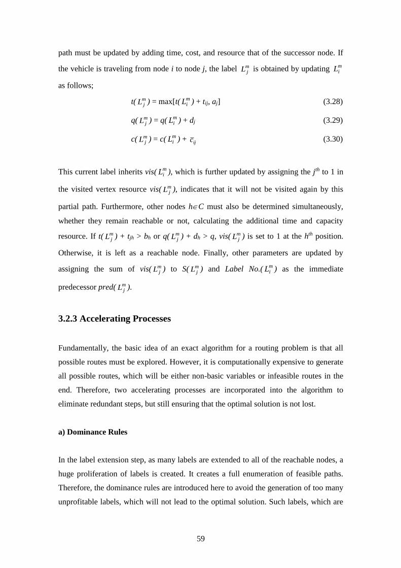
59
path must be updated by adding time, cost, and resource that of the successor node. If
the vehicle is traveling from node i to node j, the label mjL is obtained by updating m
iL
as follows;
t( mjL ) = max[t( m
iL ) + tij, aj] (3.28)
q( mjL ) = q( m
iL ) + dj (3.29)
c( mjL ) = c( m
iL ) + ijc (3.30)
This current label inherits vis( miL ), which is further updated by assigning the jth to 1 in
the visited vertex resource vis( mjL ), indicates that it will not be visited again by this
partial path. Furthermore, other nodes hC must also be determined simultaneously,
whether they remain reachable or not, calculating the additional time and capacity
resource. If t( mjL ) + tjh > bh or q( m
jL ) + dh > q, vis( mjL ) is set to 1 at the hth position.
Otherwise, it is left as a reachable node. Finally, other parameters are updated by
assigning the sum of vis( mjL ) to S( m
jL ) and Label No.( miL ) as the immediate
predecessor pred( mjL ).
3.2.3 Accelerating Processes
Fundamentally, the basic idea of an exact algorithm for a routing problem is that all
possible routes must be explored. However, it is computationally expensive to generate
all possible routes, which will be either non-basic variables or infeasible routes in the
end. Therefore, two accelerating processes are incorporated into the algorithm to
eliminate redundant steps, but still ensuring that the optimal solution is not lost.
a) Dominance Rules
In the label extension step, as many labels are extended to all of the reachable nodes, a
huge proliferation of labels is created. It creates a full enumeration of feasible paths.
Therefore, the dominance rules are introduced here to avoid the generation of too many
unprofitable labels, which will not lead to the optimal solution. Such labels, which are
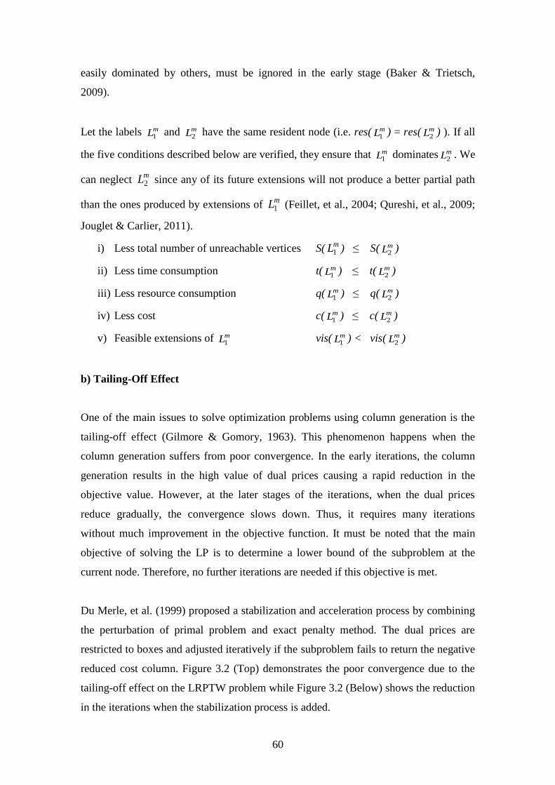
60
easily dominated by others, must be ignored in the early stage (Baker & Trietsch,
2009).
Let the labels mL1 and mL2
have the same resident node (i.e. res( mL1) = res( mL2
) ). If all
the five conditions described below are verified, they ensure that mL1 dominates mL2 . We
can neglect mL2 since any of its future extensions will not produce a better partial path
than the ones produced by extensions of mL1 (Feillet, et al., 2004; Qureshi, et al., 2009;
Jouglet & Carlier, 2011).
i) Less total number of unreachable vertices S(mL1 ) ≤ S( mL2 )
ii) Less time consumption t( mL1 ) ≤ t( mL2 )
iii) Less resource consumption q( mL1 ) ≤ q( mL2 )
iv) Less cost c( mL1 ) ≤ c( mL2 )
v) Feasible extensions of mL1 vis( mL1 ) < vis( mL2 )
b) Tailing-Off Effect
One of the main issues to solve optimization problems using column generation is the
tailing-off effect (Gilmore & Gomory, 1963). This phenomenon happens when the
column generation suffers from poor convergence. In the early iterations, the column
generation results in the high value of dual prices causing a rapid reduction in the
objective value. However, at the later stages of the iterations, when the dual prices
reduce gradually, the convergence slows down. Thus, it requires many iterations
without much improvement in the objective function. It must be noted that the main
objective of solving the LP is to determine a lower bound of the subproblem at the
current node. Therefore, no further iterations are needed if this objective is met.
Du Merle, et al. (1999) proposed a stabilization and acceleration process by combining
the perturbation of primal problem and exact penalty method. The dual prices are
restricted to boxes and adjusted iteratively if the subproblem fails to return the negative
reduced cost column. Figure 3.2 (Top) demonstrates the poor convergence due to the
tailing-off effect on the LRPTW problem while Figure 3.2 (Below) shows the reduction
in the iterations when the stabilization process is added.
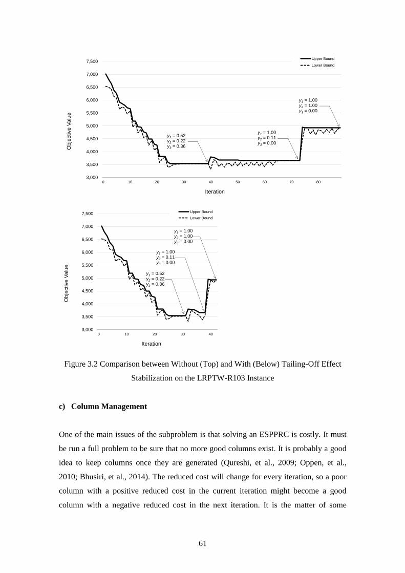
61
Figure 3.2 Comparison between Without (Top) and With (Below) Tailing-Off Effect
Stabilization on the LRPTW-R103 Instance
c) Column Management
One of the main issues of the subproblem is that solving an ESPPRC is costly. It must
be run a full problem to be sure that no more good columns exist. It is probably a good
idea to keep columns once they are generated (Qureshi, et al., 2009; Oppen, et al.,
2010; Bhusiri, et al., 2014). The reduced cost will change for every iteration, so a poor
column with a positive reduced cost in the current iteration might become a good
column with a negative reduced cost in the next iteration. It is the matter of some
3,000
3,500
4,000
4,500
5,000
5,500
6,000
6,500
7,000
7,500
0 10 20 30 40 50 60 70 80
Obje
ctive V
alu
e
Iteration
Upper Bound
Lower Bound
y1 = 0.52y2 = 0.22y3 = 0.36
y1 = 1.00y2 = 0.11y3 = 0.00
y1 = 1.00y2 = 1.00y3 = 0.00
3,000
3,500
4,000
4,500
5,000
5,500
6,000
6,500
7,000
7,500
0 10 20 30 40
Obje
ctive V
alu
e
Iteration
Upper Bound
Lower Bound
y1 = 0.52y2 = 0.22y3 = 0.36
y1 = 1.00y2 = 0.11y3 = 0.00
y1 = 1.00y2 = 1.00y3 = 0.00
62
aspects to consider about generating new columns, keeping old ones, and how many to
add to the restricted master.
3.2.4 Branching Strategies
The major issue with integer problems is that the feasible region is not a convex set,
which is an important feature of an LP and the key to the good performance of the
simplex algorithm. The feasible region of an IP is a set of points, and the number of
points or solutions for a bounded IP is finite. However, integer problems are
nevertheless much harder than LPs. There is no integer version of the simplex
algorithm that leads us towards the optimal solution by visiting a series of feasible
solutions with increasingly good objective function values (Oppen, et al., 2010). To
avoid ends up with that enumeration, therefore, the branch-and-bound algorithm is
introduced in this step.
The branch-and-bound was first proposed by Land and Doig (1960) for discrete
programming and has become the most commonly used tool for solving NP-hard
optimization problems (Clausen, 1999). The algorithm explores branches of this tree,
which represent subsets of the solution set. Before enumerating the candidate solutions
of a branch, the branch is checked against upper and lower estimated bounds on the
optimal solution. It is discarded if it cannot produce a better solution than the best one
found so far by the algorithm. While the subproblem is solved, one of the following
situation occur as the branching rules (Oppen, et al., 2010);
1. If the solution is fractional with a better objective value than the current
candidate solution, choose a variable with a fractional value to branch on, and
create two (or more) subproblems.
2. If the solution has a poorer or equal value than the current candidate solution,
the node is fathomed.
3. If the solution is an integer with a better objective value than the candidate
solution, the solution becomes the new candidate solution, and the node is
fathomed.
4. If no feasible solution, the node is fathomed.
63
In our case, when subproblem does not generate any more negative reduced cost
columns, the master problem provides the optimal solution of the set covering type
formulation. If all decision variables, ym, xijk, are an integer, the solution is also
optimum. However, if any of those variables have fractional values or some customers
may be visited more than once, the branch-and-bound tree must be explored.
The branching strategies is very importance in a branch-and-price algorithm because
branching decisions are taken regarding the fractional solutions of the generated
columns. These decisions must be compatible with the structure of the subproblem for
generating the new columns (Desrochers, et al., 1992). The depth-first, branch and
bound algorithm is used if the LP solution is fractional. Three branching schemes are
applied in the branch-and-price algorithm for solving the LRPTW.
a) Facility Variables
If at least one of the facility variable ym presents fractional value, it simply forces
corresponding depot to be closed or open by assigning the value 0 or 1, respectively.
The pricing problem remains the same since ym is not present in any constraints of the
subproblem where each depot is considered independently.
b) Number of Vehicles
Let km is the number of vehicles stationed at facility m. If the solution contains a
fractional number of these vehicles, let’s say l, it can be either round up or round down
by adding the covering constraints km ≥ l or km ≤ l in constraint (3.16). This process
is repeated everywhere if it is needed in the branch-and-bound tree.
c) Flow Variables
The branching on flow variables (xijk) is used if both the number of open facilities and
the number of vehicles are integers, but the flow variables are still fractional
(Kallenhauge, et al., 2005). Equation (3.29) is used to make a decision for the
branching arc.
max cij [min(xijk, 1- xijk)] (3.31)
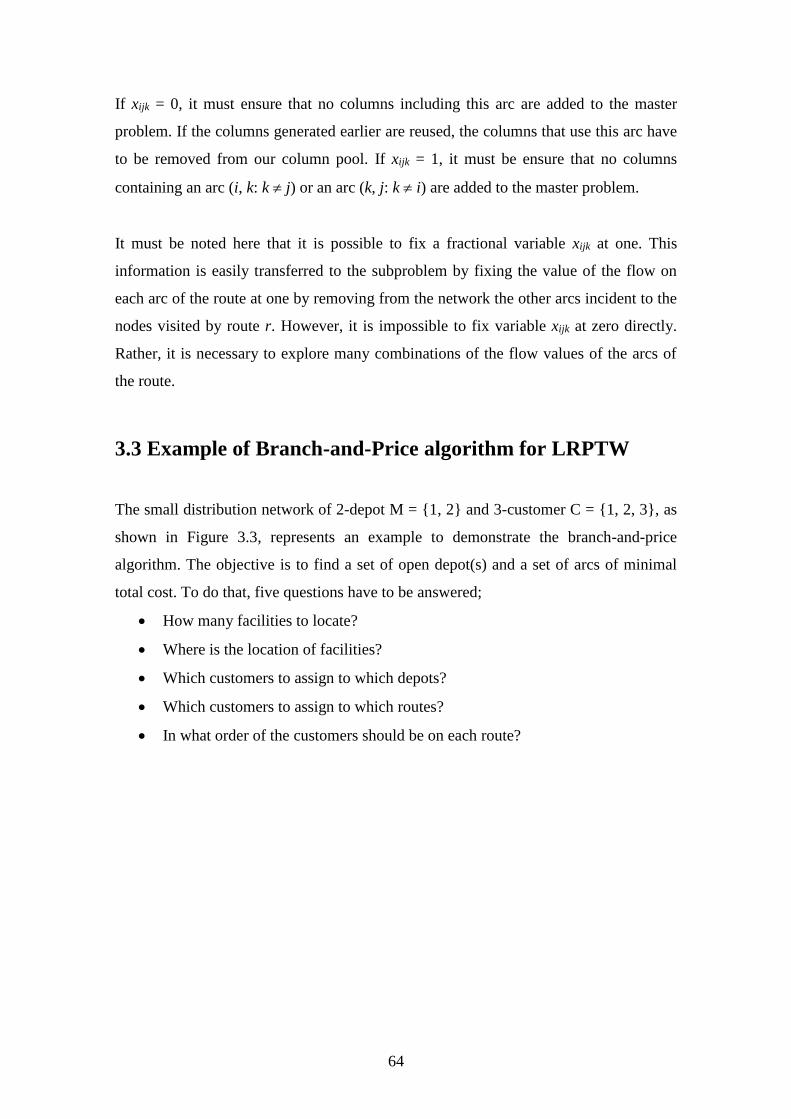
64
If xijk = 0, it must ensure that no columns including this arc are added to the master
problem. If the columns generated earlier are reused, the columns that use this arc have
to be removed from our column pool. If xijk = 1, it must be ensure that no columns
containing an arc (i, k: k j) or an arc (k, j: k i) are added to the master problem.
It must be noted here that it is possible to fix a fractional variable xijk at one. This
information is easily transferred to the subproblem by fixing the value of the flow on
each arc of the route at one by removing from the network the other arcs incident to the
nodes visited by route r. However, it is impossible to fix variable xijk at zero directly.
Rather, it is necessary to explore many combinations of the flow values of the arcs of
the route.
3.3 Example of Branch-and-Price algorithm for LRPTW
The small distribution network of 2-depot M = {1, 2} and 3-customer C = {1, 2, 3}, as
shown in Figure 3.3, represents an example to demonstrate the branch-and-price
algorithm. The objective is to find a set of open depot(s) and a set of arcs of minimal
total cost. To do that, five questions have to be answered;
How many facilities to locate?
Where is the location of facilities?
Which customers to assign to which depots?
Which customers to assign to which routes?
In what order of the customers should be on each route?
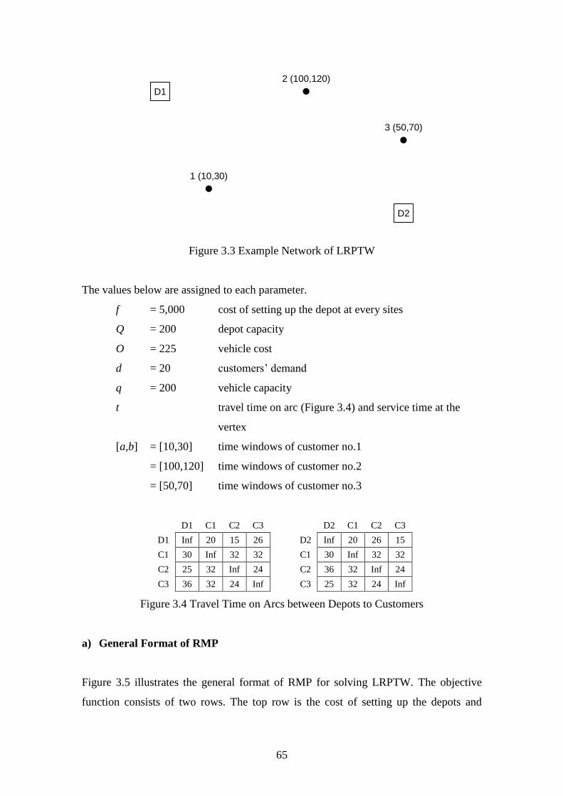
65
Figure 3.3 Example Network of LRPTW
The values below are assigned to each parameter.
f = 5,000 cost of setting up the depot at every sites
Q = 200 depot capacity
O = 225 vehicle cost
d = 20 customers’ demand
q = 200 vehicle capacity
t travel time on arc (Figure 3.4) and service time at the
vertex
[a,b] = [10,30] time windows of customer no.1
= [100,120] time windows of customer no.2
= [50,70] time windows of customer no.3
D1 C1 C2 C3
D2 C1 C2 C3
D1 Inf 20 15 26
D2 Inf 20 26 15
C1 30 Inf 32 32
C1 30 Inf 32 32
C2 25 32 Inf 24
C2 36 32 Inf 24
C3 36 32 24 Inf
C3 25 32 24 Inf
Figure 3.4 Travel Time on Arcs between Depots to Customers
a) General Format of RMP
Figure 3.5 illustrates the general format of RMP for solving LRPTW. The objective
function consists of two rows. The top row is the cost of setting up the depots and
D1
D2
1 (10,30)
2 (100,120)
3 (50,70)
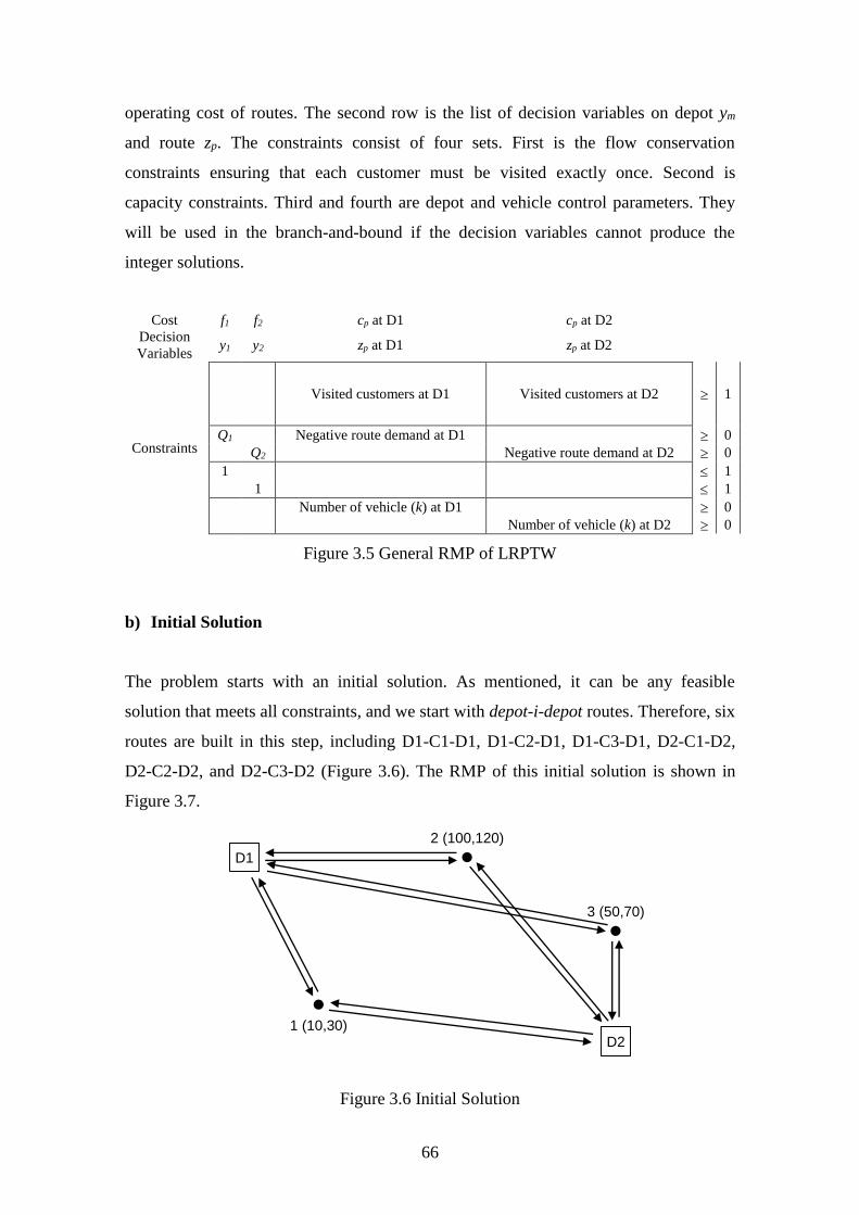
66
operating cost of routes. The second row is the list of decision variables on depot ym
and route zp. The constraints consist of four sets. First is the flow conservation
constraints ensuring that each customer must be visited exactly once. Second is
capacity constraints. Third and fourth are depot and vehicle control parameters. They
will be used in the branch-and-bound if the decision variables cannot produce the
integer solutions.
Cost f1 f2 cp at D1 cp at D2
Decision
Variables y1 y2 zp at D1 zp at D2
Constraints
Visited customers at D1 Visited customers at D2 1
Q1 Negative route demand at D1 0
Q2 Negative route demand at D2 0
1 1
1 1
Number of vehicle (k) at D1 0
Number of vehicle (k) at D2 0
Figure 3.5 General RMP of LRPTW
b) Initial Solution
The problem starts with an initial solution. As mentioned, it can be any feasible
solution that meets all constraints, and we start with depot-i-depot routes. Therefore, six
routes are built in this step, including D1-C1-D1, D1-C2-D1, D1-C3-D1, D2-C1-D2,
D2-C2-D2, and D2-C3-D2 (Figure 3.6). The RMP of this initial solution is shown in
Figure 3.7.
Figure 3.6 Initial Solution
D1
D21 (10,30)
2 (100,120)
3 (50,70)
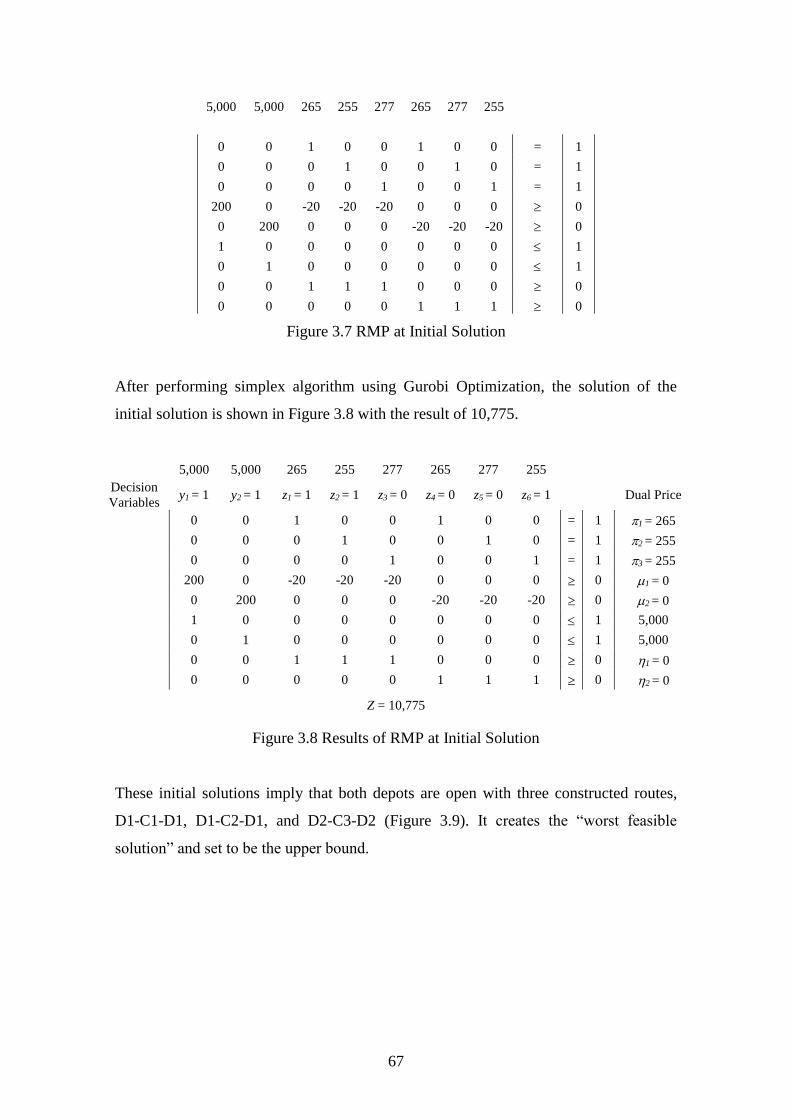
67
5,000 5,000 265 255 277 265 277 255
0 0 1 0 0 1 0 0 = 1
0 0 0 1 0 0 1 0 = 1
0 0 0 0 1 0 0 1 = 1
200 0 -20 -20 -20 0 0 0 0
0 200 0 0 0 -20 -20 -20 0
1 0 0 0 0 0 0 0 1
0 1 0 0 0 0 0 0 1
0 0 1 1 1 0 0 0 0
0 0 0 0 0 1 1 1 0
Figure 3.7 RMP at Initial Solution
After performing simplex algorithm using Gurobi Optimization, the solution of the
initial solution is shown in Figure 3.8 with the result of 10,775.
5,000 5,000 265 255 277 265 277 255
Decision
Variables y1 = 1 y2 = 1 z1 = 1 z2 = 1 z3 = 0 z4 = 0 z5 = 0 z6 = 1
Dual Price
0 0 1 0 0 1 0 0 = 1 1 = 265
0 0 0 1 0 0 1 0 = 1 2 = 255
0 0 0 0 1 0 0 1 = 1 3 = 255
200 0 -20 -20 -20 0 0 0 0 1 = 0
0 200 0 0 0 -20 -20 -20 0 2 = 0
1 0 0 0 0 0 0 0 1 5,000
0 1 0 0 0 0 0 0 1 5,000
0 0 1 1 1 0 0 0 0 1 = 0
0 0 0 0 0 1 1 1 0 2 = 0
Z = 10,775
Figure 3.8 Results of RMP at Initial Solution
These initial solutions imply that both depots are open with three constructed routes,
D1-C1-D1, D1-C2-D1, and D2-C3-D2 (Figure 3.9). It creates the “worst feasible
solution” and set to be the upper bound.
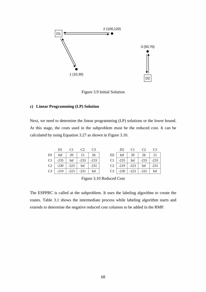
68
Figure 3.9 Initial Solution
c) Linear Programming (LP) Solution
Next, we need to determine the linear programming (LP) solutions or the lower bound.
At this stage, the costs used in the subproblem must be the reduced cost. It can be
calculated by using Equation 3.27 as shown in Figure 3.10.
D1 C1 C2 C3
D2 C1 C2 C3
D1 Inf 20 15 26
D2 Inf 20 26 15
C1 -235 Inf -233 -233
C1 -235 Inf -233 -233
C2 -230 -223 Inf -231
C2 -219 -223 Inf -231
C3 -219 -223 -231 Inf
C3 -230 -223 -231 Inf
Figure 3.10 Reduced Cost
The ESPPRC is called at the subproblem. It uses the labeling algorithm to create the
routes. Table 3.1 shows the intermediate process while labeling algorithm starts and
extends to determine the negative reduced cost columns to be added in the RMP.
D1
D21 (10,30)
2 (100,120)
3 (50,70)
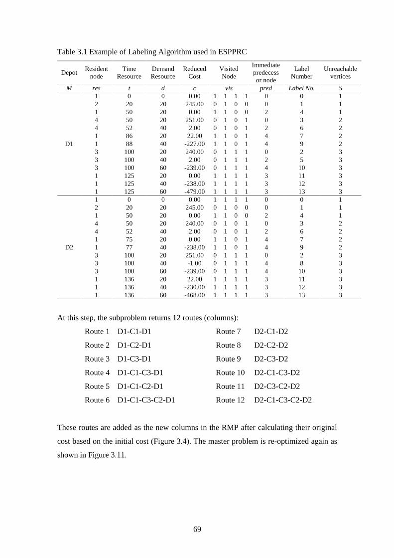
69
Table 3.1 Example of Labeling Algorithm used in ESPPRC
Depot Resident
node
Time
Resource
Demand
Resource
Reduced
Cost
Visited
Node
Immediate
predecess
or node
Label
Number
Unreachable
vertices
M res t d c vis pred Label No. S
D1
1 0 0 0.00 1 1 1 1 0 0 1
2 20 20 245.00 0 1 0 0 0 1 1
1 50 20 0.00 1 1 0 0 2 4 1
4 50 20 251.00 0 1 0 1 0 3 2
4 52 40 2.00 0 1 0 1 2 6 2
1 86 20 22.00 1 1 0 1 4 7 2
1 88 40 -227.00 1 1 0 1 4 9 2
3 100 20 240.00 0 1 1 1 0 2 3
3 100 40 2.00 0 1 1 1 2 5 3
3 100 60 -239.00 0 1 1 1 4 10 3
1 125 20 0.00 1 1 1 1 3 11 3
1 125 40 -238.00 1 1 1 1 3 12 3
1 125 60 -479.00 1 1 1 1 3 13 3
D2
1 0 0 0.00 1 1 1 1 0 0 1
2 20 20 245.00 0 1 0 0 0 1 1
1 50 20 0.00 1 1 0 0 2 4 1
4 50 20 240.00 0 1 0 1 0 3 2
4 52 40 2.00 0 1 0 1 2 6 2
1 75 20 0.00 1 1 0 1 4 7 2
1 77 40 -238.00 1 1 0 1 4 9 2
3 100 20 251.00 0 1 1 1 0 2 3
3 100 40 -1.00 0 1 1 1 4 8 3
3 100 60 -239.00 0 1 1 1 4 10 3
1 136 20 22.00 1 1 1 1 3 11 3
1 136 40 -230.00 1 1 1 1 3 12 3
1 136 60 -468.00 1 1 1 1 3 13 3
At this step, the subproblem returns 12 routes (columns):
Route 1 D1-C1-D1 Route 7 D2-C1-D2
Route 2 D1-C2-D1 Route 8 D2-C2-D2
Route 3 D1-C3-D1 Route 9 D2-C3-D2
Route 4 D1-C1-C3-D1 Route 10 D2-C1-C3-D2
Route 5 D1-C1-C2-D1 Route 11 D2-C3-C2-D2
Route 6 D1-C1-C3-C2-D1 Route 12 D2-C1-C3-C2-D2
These routes are added as the new columns in the RMP after calculating their original
cost based on the initial cost (Figure 3.4). The master problem is re-optimized again as
shown in Figure 3.11.
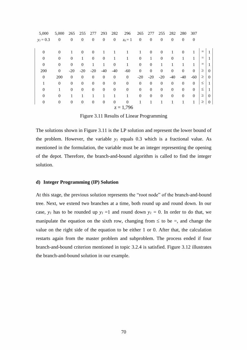
70
5,000 5,000 265 255 277 293 282 296 265 277 255 282 280 307
y1 = 0.3 0 0 0 0 0 0 z6 = 1 0 0 0 0 0 0
0 0 1 0 0 1 1 1 1 0 0 1 0 1 = 1
0 0 0 1 0 0 1 1 0 1 0 0 1 1 = 1
0 0 0 0 1 1 0 1 0 0 1 1 1 1 = 1
200 0 -20 -20 -20 -40 -40 -60 0 0 0 0 0 0 0
0 200 0 0 0 0 0 0 -20 -20 -20 -40 -40 -60 0
1 0 0 0 0 0 0 0 0 0 0 0 0 0 1
0 1 0 0 0 0 0 0 0 0 0 0 0 0 1
0 0 1 1 1 1 1 1 0 0 0 0 0 0 0
0 0 0 0 0 0 0 0 1 1 1 1 1 1 0
z = 1,796
Figure 3.11 Results of Linear Programming
The solutions shown in Figure 3.11 is the LP solution and represent the lower bound of
the problem. However, the variable y1 equals 0.3 which is a fractional value. As
mentioned in the formulation, the variable must be an integer representing the opening
of the depot. Therefore, the branch-and-bound algorithm is called to find the integer
solution.
d) Integer Programming (IP) Solution
At this stage, the previous solution represents the “root node” of the branch-and-bound
tree. Next, we extend two branches at a time, both round up and round down. In our
case, y1 has to be rounded up y1 =1 and round down y1 = 0. In order to do that, we
manipulate the equation on the sixth row, changing from to be =, and change the
value on the right side of the equation to be either 1 or 0. After that, the calculation
restarts again from the master problem and subproblem. The process ended if four
branch-and-bound criterion mentioned in topic 3.2.4 is satisfied. Figure 3.12 illustrates
the branch-and-bound solution in our example.
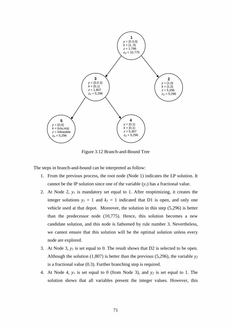
71
Figure 3.12 Branch-and-Bound Tree
The steps in branch-and-bound can be interpreted as follow:
1. From the previous process, the root node (Node 1) indicates the LP solution. It
cannot be the IP solution since one of the variable (y1) has a fractional value.
2. At Node 2, y1 is mandatory set equal to 1. After reoptimizing, it creates the
integer solutions y1 = 1 and k1 = 1 indicated that D1 is open, and only one
vehicle used at that depot. Moreover, the solution in this step (5,296) is better
than the predecessor node (10,775). Hence, this solution becomes a new
candidate solution, and this node is fathomed by rule number 3. Nevertheless,
we cannot ensure that this solution will be the optimal solution unless every
node are explored.
3. At Node 3, y1 is set equal to 0. The result shows that D2 is selected to be open.
Although the solution (1,807) is better than the previous (5,296), the variable y2
is a fractional value (0.3). Further branching step is required.
4. At Node 4, y1 is set equal to 0 (from Node 3), and y2 is set equal to 1. The
solution shows that all variables present the integer values. However, this
1 y = {0.3,0} k = {1, 0} z = 1,796
zip = 10,775
2 y = {1,0} k = {1,0} z = 5,296 zip = 5,296
3 y = {0,0.3} k = {0,1} z = 1,807 zip = 5,296
4 y = {0,1} k = {0,1} z = 5,307 zip = 5,296
5 y = {0,0} k = {n/a,n/a} z = Infeasible zip = 5,296
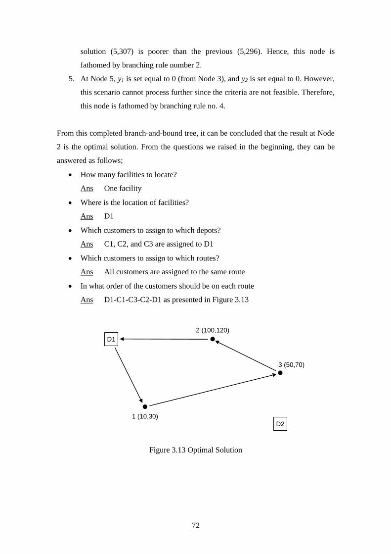
72
solution (5,307) is poorer than the previous (5,296). Hence, this node is
fathomed by branching rule number 2.
5. At Node 5, y1 is set equal to 0 (from Node 3), and y2 is set equal to 0. However,
this scenario cannot process further since the criteria are not feasible. Therefore,
this node is fathomed by branching rule no. 4.
From this completed branch-and-bound tree, it can be concluded that the result at Node
2 is the optimal solution. From the questions we raised in the beginning, they can be
answered as follows;
How many facilities to locate?
Ans One facility
Where is the location of facilities?
Ans D1
Which customers to assign to which depots?
Ans C1, C2, and C3 are assigned to D1
Which customers to assign to which routes?
Ans All customers are assigned to the same route
In what order of the customers should be on each route
Ans D1-C1-C3-C2-D1 as presented in Figure 3.13
Figure 3.13 Optimal Solution
D1
D21 (10,30)
2 (100,120)
3 (50,70)
73
References
Baker, K. & Trietsch, D., 2009. Principles of Sequencing and Scheduling. New Jersey:
John Wiley & Sons, Inc.
Bhusiri, N., Qureshi, A. G. & Taniguchi, E., 2014. The trade-off between fixed vehicle
costs and time-dependent arrival penalties in a routing problem. Transportation
Research Part E: Logistics and Transportation Review, Volume 62, pp. 1-22.
Clausen, J., 1999. Branch and bound algorithms-principles and examples, Copenhagen:
Department of Computer Science, University of Copenhagen.
Dantzig, G. B. & Wolfe, P., 1960. Decomposition principle for linear programs.
Operations Research, 8(1), pp. 101-111.
Desaulniers, G., Lessard, F. & Hadjar, A., 2008. Tabu search, partial elementarity, and
generalized k-path inequalities for the vehicle routing problem with time windows.
Transportation Science, 42(3), pp. 387-404.
Desrochers, M., 1988. An Algorithm for the Shortest Path Problem with Resource
Constraints, s.l.: Technical Report G-88-27, GERAD.
Desrochers, M., Desrosiers, J. & Solomon, M., 1992. A new optimization algorithm for
the vehicle routing problem with time windows. Operations Research, 40(2), pp.
342-354.
Desrosiers, J., Soumis, F. & Desrochers, M., 1984. Routing with time windows by
column generation. Networks, 14(4), pp. 545-565.
Dijkstra, E. W., 1959. A note on two problems in connexion with graphs. Numerische
mathematik, 1(1), pp. 269-271.
Du Merle, O., Villeneuve, D., Desrosiers, J. & Hansen, P., 1999. Stabilized column
generation. Discrete Mathematics, 194(1), pp. 229-237.
Feillet, D., Dejax, P., Gendreau, M. & Gueguen, C., 2004. An exact algorithm for the
elementary shortest path problem with resource constraints: Application to some
vehicle routing problems. Network, 44(3), pp. 216-229.
Gendreau, M. & Potvin, J. Y., 2010. Handbook of metaheuristics. Vol. 2 ed. New York:
Springer.
Gilmore, P. C. & Gomory, R. E., 1963. A linear programming approach to the cutting
stock problem-Part II. Operations Research, 11(6), pp. 863-888.
74
Glover, F., 1977. Heuristics for integer programming using surrogate constraints.
Decision Sciences, 8(1), pp. 156-166.
Glover, F. & Laguna, M., 1997. Tabu search. Massachusetts: Kluwer Academic
Publishers.
Jouglet, A. & Carlier, J., 2011. Dominance rules in combinatorial optimization
problems. European Journal of Operational Research, 212(3), pp. 433-444.
Kallenhauge, B., Larsen, J., Madsen, O. & Solomon, M., 2005. Vehicle Routing
Problem with Time Windows. In: G. Desaulniers, J. Desrosiers & M. M. Solomon,
eds. Column Generation. New York: Springer.
Land, A. H. & Doig, A. G., 1960. An automatic method of solving discrete
programming problems. Econometrica: Journal of the Econometric Society, pp.
497-520.
Lübbecke, M. E. & Desrosiers, J., 2005. Selected topics in column generation.
Operations Research, 53(6), pp. 1007-1023.
Nagy, G. & Salhi, S., 1996. Nested heuristic methods for the location-routeing
problem. Journal of the Operational Research Society, Volume 47, pp. 1166-1174.
Oppen, J., Løkketangen, A. & Desrosiers, J., 2010. Solving a rich vehicle routing and
inventory problem using column generation. Computers & Operations Research,
37(7), pp. 1308-1317.
Osman, I. H., 1993. Metastrategy simulated annealing and tabu search algorithms for
the vehicle routing problem. Annals of operations research, 41(4), pp. 421-451.
Perrot, N., 2005. Integer Programming Column Generation Strategies for the Cutting
Stock Problem and its Variants, Bordeaux: PhD Thesis, University of Bordeaux.
Qureshi, A., Taniguchi, E. & Yamada, T., 2009. An Exact Solution Approach for
Vehicle Routing and Scheduling Problem with Soft Time Windows. Transportation
Research Part E: Logistics and Transportation Review, 45(6), pp. 960-977.
Righini, G. & Salani, M., 2008. New dynamic programming algorithms for the resource
constrained elementary shortest path problem. Networks, 51(3), pp. 155-170.
Savelsbergh, M. W., 1992. The vehicle routing problem with time windows:
Minimizing route duration. ORSA Journal on computing, 4(2), pp. 146-154.
Toth, P. & Vigo, D., 2002. Capacitated vehicle-routing problems in the vehicle-routing
problem. SIAM monographs on discrete mathematics and applications.
Tuzun, D. & Burke, L. I., 1999. A two-phase tabu search approach to the location
routing problem. European Journal of Operational Research, 116(1), pp. 87-99.
75
Chapter 4
Model Evaluation
4.1 Modified Solomon Benchmark
4.2 Result and Discussion
4.2.1 Computational Time
4.2.2 Cost Components
References

76
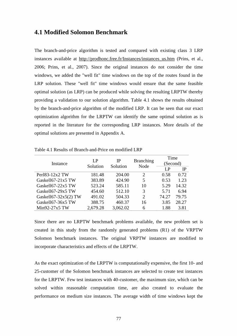
77
4.1 Modified Solomon Benchmark
The branch-and-price algorithm is tested and compared with existing class 3 LRP
instances available at http://prodhonc.free.fr/Instances/instances_us.htm (Prins, et al.,
2006; Prins, et al., 2007). Since the original instances do not consider the time
windows, we added the "well fit" time windows on the top of the routes found in the
LRP solution. These "well fit" time windows would ensure that the same feasible
optimal solution (as LRP) can be produced while solving the resulting LRPTW thereby
providing a validation to our solution algorithm. Table 4.1 shows the results obtained
by the branch-and-price algorithm of the modified LRP. It can be seen that our exact
optimization algorithm for the LRPTW can identify the same optimal solution as is
reported in the literature for the corresponding LRP instances. More details of the
optimal solutions are presented in Appendix A.
Table 4.1 Results of Branch-and-Price on modified LRP
Instance LP
Solution
IP
Solution
Branching
Node
Time
(Second)
LP IP
Perl83-12x2 TW 181.48 204.00 2 0.58 0.72
Gaskell67-21x5 TW 383.89 424.90 5 0.53 1.23
Gaskell67-22x5 TW 523.24 585.11 10 5.29 14.32
Gaskell67-29x5 TW 454.60 512.10 3 5.71 6.94
Gaskell67-32x5(2) TW 491.02 504.33 2 74.27 79.75
Gaskell67-36x5 TW 388.75 460.37 16 3.85 28.27
Min92-27x5 TW 2,679.28 3,062.02 6 1.88 3.81
Since there are no LRPTW benchmark problems available, the new problem set is
created in this study from the randomly generated problems (R1) of the VRPTW
Solomon benchmark instances. The original VRPTW instances are modified to
incorporate characteristics and effects of the LRPTW.
As the exact optimization of the LRPTW is computationally expensive, the first 10- and
25-customer of the Solomon benchmark instances are selected to create test instances
for the LRPTW. Few test instances with 40-customer, the maximum size, which can be
solved within reasonable computation time, are also created to evaluate the
performance on medium size instances. The average width of time windows kept the
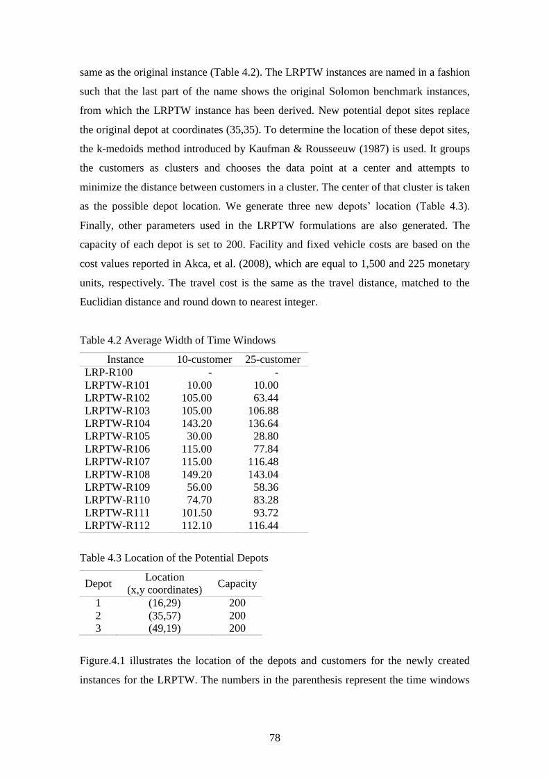
78
same as the original instance (Table 4.2). The LRPTW instances are named in a fashion
such that the last part of the name shows the original Solomon benchmark instances,
from which the LRPTW instance has been derived. New potential depot sites replace
the original depot at coordinates (35,35). To determine the location of these depot sites,
the k-medoids method introduced by Kaufman & Rousseeuw (1987) is used. It groups
the customers as clusters and chooses the data point at a center and attempts to
minimize the distance between customers in a cluster. The center of that cluster is taken
as the possible depot location. We generate three new depots’ location (Table 4.3).
Finally, other parameters used in the LRPTW formulations are also generated. The
capacity of each depot is set to 200. Facility and fixed vehicle costs are based on the
cost values reported in Akca, et al. (2008), which are equal to 1,500 and 225 monetary
units, respectively. The travel cost is the same as the travel distance, matched to the
Euclidian distance and round down to nearest integer.
Table 4.2 Average Width of Time Windows
Instance 10-customer 25-customer
LRP-R100 - -
LRPTW-R101 10.00 10.00
LRPTW-R102 105.00 63.44
LRPTW-R103 105.00 106.88
LRPTW-R104 143.20 136.64
LRPTW-R105 30.00 28.80
LRPTW-R106 115.00 77.84
LRPTW-R107 115.00 116.48
LRPTW-R108 149.20 143.04
LRPTW-R109 56.00 58.36
LRPTW-R110 74.70 83.28
LRPTW-R111 101.50 93.72
LRPTW-R112 112.10 116.44
Table 4.3 Location of the Potential Depots
Depot Location
(x,y coordinates) Capacity
1 (16,29) 200
2 (35,57) 200
3 (49,19) 200
Figure.4.1 illustrates the location of the depots and customers for the newly created
instances for the LRPTW. The numbers in the parenthesis represent the time windows
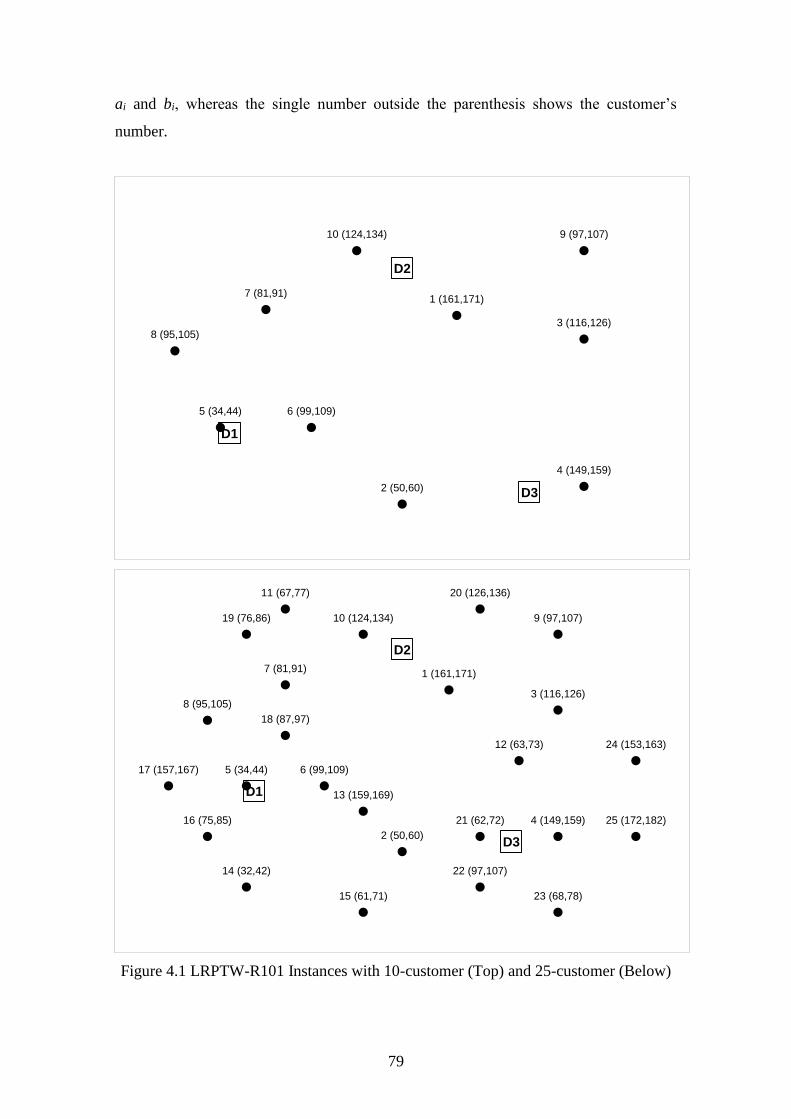
79
ai and bi, whereas the single number outside the parenthesis shows the customer’s
number.
Figure 4.1 LRPTW-R101 Instances with 10-customer (Top) and 25-customer (Below)
1 (161,171)
2 (50,60)
3 (116,126)
4 (149,159)
5 (34,44) 6 (99,109)
7 (81,91)
8 (95,105)
9 (97,107)10 (124,134)
D1
D2
D3
1 (161,171)
2 (50,60)
3 (116,126)
4 (149,159)
5 (34,44) 6 (99,109)
7 (81,91)
8 (95,105)
9 (97,107)10 (124,134)
11 (67,77)
12 (63,73)
13 (159,169)
14 (32,42)
15 (61,71)
16 (75,85)
17 (157,167)
18 (87,97)
19 (76,86)
20 (126,136)
21 (62,72)
22 (97,107)
23 (68,78)
24 (153,163)
25 (172,182)
D1
D2
D3
80
4.2 Results and Discussion
Computational tests of the algorithm are performed on a computer with Intel® Core™
i7-3930K 3.20 GHz processor, and 32 GB of RAM. The algorithm is programmed in
MATLAB with Gurobi Optimizer 5.6 as the LP solver.
The results are shown in Table 4.4. The column “LP Solution” refers to the linear
programming solution at the root node while column “IP Solution” is the optimal
integer solution. Column “Branching Node” means the number of nodes in the branch-
and-bound tree from the root node to reach the optimal solution. “Time” shows the
computational time. In “Selected Depot” column, the check mark means that the depot
is selected. “Number of Vehicles” refers to the number of vehicles used in each selected
depot and “Number of Customers” equals to the number of customers served by the
particular depot.
Furthermore, “Total Distance” refers to the total traveling distance starting from the
depot to visit all of the customers and return to the depot again and “Average
Distances” means the average distances traveled by each vehicle. “Total Load”
represents the total units of the commodity delivered by vehicles. In other words, this
value equals to customers’ demand along the vehicle route. “Average Load” is the
average units of a commodity containing by each vehicle. “Load Factor” equals to total
load divide by vehicle capacity. Finally, the last three columns, i.e. depot, vehicle, and
transport costs are the fragments of the total cost. Their summation is equal to the IP
solution.
The results show that our algorithm is successful in solving LRPTW in all instances
optimally with acceptable times. Moreover, three instances with 40-customer are also
successfully solved under eight-hour limitation time. More details of the optimal
solutions are presented in Appendix B.
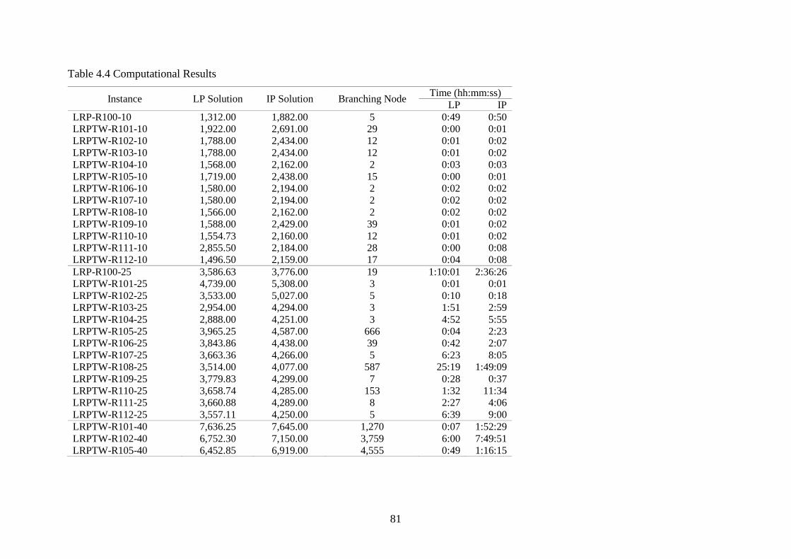
81
Table 4.4 Computational Results
Instance LP Solution IP Solution Branching Node Time (hh:mm:ss)
LP IP
LRP-R100-10 1,312.00 1,882.00 5 0:49 0:50
LRPTW-R101-10 1,922.00 2,691.00 29 0:00 0:01
LRPTW-R102-10 1,788.00 2,434.00 12 0:01 0:02
LRPTW-R103-10 1,788.00 2,434.00 12 0:01 0:02
LRPTW-R104-10 1,568.00 2,162.00 2 0:03 0:03
LRPTW-R105-10 1,719.00 2,438.00 15 0:00 0:01
LRPTW-R106-10 1,580.00 2,194.00 2 0:02 0:02
LRPTW-R107-10 1,580.00 2,194.00 2 0:02 0:02
LRPTW-R108-10 1,566.00 2,162.00 2 0:02 0:02
LRPTW-R109-10 1,588.00 2,429.00 39 0:01 0:02
LRPTW-R110-10 1,554.73 2,160.00 12 0:01 0:02
LRPTW-R111-10 2,855.50 2,184.00 28 0:00 0:08
LRPTW-R112-10 1,496.50 2,159.00 17 0:04 0:08
LRP-R100-25 3,586.63 3,776.00 19 1:10:01 2:36:26
LRPTW-R101-25 4,739.00 5,308.00 3 0:01 0:01
LRPTW-R102-25 3,533.00 5,027.00 5 0:10 0:18
LRPTW-R103-25 2,954.00 4,294.00 3 1:51 2:59
LRPTW-R104-25 2,888.00 4,251.00 3 4:52 5:55
LRPTW-R105-25 3,965.25 4,587.00 666 0:04 2:23
LRPTW-R106-25 3,843.86 4,438.00 39 0:42 2:07
LRPTW-R107-25 3,663.36 4,266.00 5 6:23 8:05
LRPTW-R108-25 3,514.00 4,077.00 587 25:19 1:49:09
LRPTW-R109-25 3,779.83 4,299.00 7 0:28 0:37
LRPTW-R110-25 3,658.74 4,285.00 153 1:32 11:34
LRPTW-R111-25 3,660.88 4,289.00 8 2:27 4:06
LRPTW-R112-25 3,557.11 4,250.00 5 6:39 9:00
LRPTW-R101-40 7,636.25 7,645.00 1,270 0:07 1:52:29
LRPTW-R102-40 6,752.30 7,150.00 3,759 6:00 7:49:51
LRPTW-R105-40 6,452.85 6,919.00 4,555 0:49 1:16:15
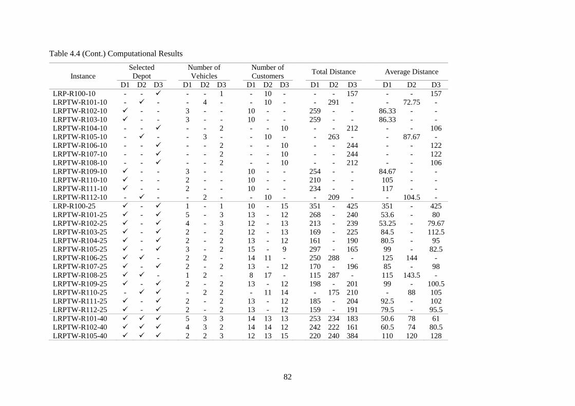
82
Table 4.4 (Cont.) Computational Results
Instance
Selected
Depot
Number of
Vehicles
Number of
Customers
Total Distance
Average Distance
D1 D2 D3
D1 D2 D3
D1 D2 D3
D1 D2 D3
D1 D2 D3
LRP-R100-10 - -
- - 1
- 10 -
- - 157
- - 157
LRPTW-R101-10 - -
- 4 -
- 10 -
- 291 -
- 72.75 -
LRPTW-R102-10 - -
3 - -
10 - -
259 - -
86.33 - -
LRPTW-R103-10 - -
3 - -
10 - -
259 - -
86.33 - -
LRPTW-R104-10 - -
- - 2
- - 10
- - 212
- - 106
LRPTW-R105-10 - -
- 3 -
- 10 -
- 263 -
- 87.67 -
LRPTW-R106-10 - -
- - 2
- - 10
- - 244
- - 122
LRPTW-R107-10 - -
- - 2
- - 10
- - 244
- - 122
LRPTW-R108-10 - -
- - 2
- - 10
- - 212
- - 106
LRPTW-R109-10 - -
3 - -
10 - -
254 - -
84.67 - -
LRPTW-R110-10 - -
2 - -
10 - -
210 - -
105 - -
LRPTW-R111-10 - -
2 - -
10 - -
234 - -
117 - -
LRPTW-R112-10 - -
- 2 -
- 10 -
- 209 -
- 104.5 -
LRP-R100-25 -
1 - 1
10 - 15
351 - 425
351 - 425
LRPTW-R101-25 -
5 - 3
13 - 12
268 - 240
53.6 - 80
LRPTW-R102-25 -
4 - 3
12 - 13
213 - 239
53.25 - 79.67
LRPTW-R103-25 -
2 - 2
12 - 13
169 - 225
84.5 - 112.5
LRPTW-R104-25 -
2 - 2
13 - 12
161 - 190
80.5 - 95
LRPTW-R105-25 -
3 - 2
15 - 9
297 - 165
99 - 82.5
LRPTW-R106-25 -
2 2 -
14 11 -
250 288 -
125 144 -
LRPTW-R107-25 -
2 - 2
13 - 12
170 - 196
85 - 98
LRPTW-R108-25 -
1 2 -
8 17 -
115 287 -
115 143.5 -
LRPTW-R109-25 -
2 - 2
13 - 12
198 - 201
99 - 100.5
LRPTW-R110-25 -
- 2 2
- 11 14
- 175 210
- 88 105
LRPTW-R111-25 -
2 - 2
13 - 12
185 - 204
92.5 - 102
LRPTW-R112-25 -
2 - 2
13 - 12
159 - 191
79.5 - 95.5
LRPTW-R101-40
5 3 3
14 13 13
253 234 183
50.6 78 61
LRPTW-R102-40
4 3 2
14 14 12
242 222 161
60.5 74 80.5
LRPTW-R105-40
2 2 3
12 13 15
220 240 384
110 120 128
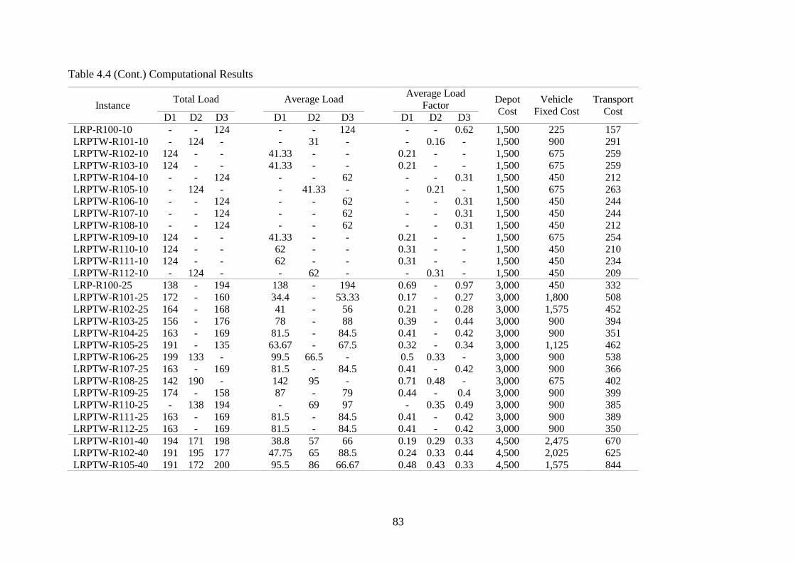
83
Table 4.4 (Cont.) Computational Results
Instance Total Load
Average Load
Average Load
Factor
Depot
Cost
Vehicle
Fixed Cost
Transport
Cost D1 D2 D3
D1 D2 D3
D1 D2 D3
LRP-R100-10 - - 124
- - 124
- - 0.62
1,500 225 157
LRPTW-R101-10 - 124 -
- 31 -
- 0.16 -
1,500 900 291
LRPTW-R102-10 124 - -
41.33 - -
0.21 - -
1,500 675 259
LRPTW-R103-10 124 - -
41.33 - -
0.21 - -
1,500 675 259
LRPTW-R104-10 - - 124
- - 62
- - 0.31
1,500 450 212
LRPTW-R105-10 - 124 -
- 41.33 -
- 0.21 -
1,500 675 263
LRPTW-R106-10 - - 124
- - 62
- - 0.31
1,500 450 244
LRPTW-R107-10 - - 124
- - 62
- - 0.31
1,500 450 244
LRPTW-R108-10 - - 124
- - 62
- - 0.31
1,500 450 212
LRPTW-R109-10 124 - -
41.33 - -
0.21 - -
1,500 675 254
LRPTW-R110-10 124 - -
62 - -
0.31 - -
1,500 450 210
LRPTW-R111-10 124 - -
62 - -
0.31 - -
1,500 450 234
LRPTW-R112-10 - 124 -
- 62 -
- 0.31 -
1,500 450 209
LRP-R100-25 138 - 194
138 - 194
0.69 - 0.97
3,000 450 332
LRPTW-R101-25 172 - 160
34.4 - 53.33
0.17 - 0.27
3,000 1,800 508
LRPTW-R102-25 164 - 168
41 - 56
0.21 - 0.28
3,000 1,575 452
LRPTW-R103-25 156 - 176
78 - 88
0.39 - 0.44
3,000 900 394
LRPTW-R104-25 163 - 169
81.5 - 84.5
0.41 - 0.42
3,000 900 351
LRPTW-R105-25 191 - 135
63.67 - 67.5
0.32 - 0.34
3,000 1,125 462
LRPTW-R106-25 199 133 -
99.5 66.5 -
0.5 0.33 -
3,000 900 538
LRPTW-R107-25 163 - 169
81.5 - 84.5
0.41 - 0.42
3,000 900 366
LRPTW-R108-25 142 190 -
142 95 -
0.71 0.48 -
3,000 675 402
LRPTW-R109-25 174 - 158
87 - 79
0.44 - 0.4
3,000 900 399
LRPTW-R110-25 - 138 194
- 69 97
- 0.35 0.49
3,000 900 385
LRPTW-R111-25 163 - 169
81.5 - 84.5
0.41 - 0.42
3,000 900 389
LRPTW-R112-25 163 - 169
81.5 - 84.5
0.41 - 0.42
3,000 900 350
LRPTW-R101-40 194 171 198
38.8 57 66
0.19 0.29 0.33
4,500 2,475 670
LRPTW-R102-40 191 195 177
47.75 65 88.5
0.24 0.33 0.44
4,500 2,025 625
LRPTW-R105-40 191 172 200
95.5 86 66.67
0.48 0.43 0.33
4,500 1,575 844
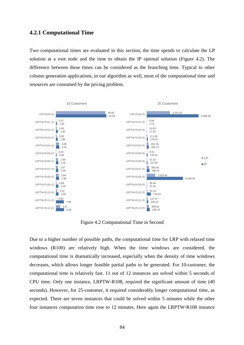
84
4.2.1 Computational Time
Two computational times are evaluated in this section; the time spends to calculate the LP
solution at a root node and the time to obtain the IP optimal solution (Figure 4.2). The
difference between these times can be considered as the branching time. Typical to other
column generation applications, in our algorithm as well, most of the computational time and
resources are consumed by the pricing problem.
Figure 4.2 Computational Time in Second
Due to a higher number of possible paths, the computational time for LRP with relaxed time
windows (R100) are relatively high. When the time windows are considered, the
computational time is dramatically increased, especially when the density of time windows
decreases, which allows longer feasible partial paths to be generated. For 10-customer, the
computational time is relatively fast. 11 out of 12 instances are solved within 5 seconds of
CPU time. Only one instance, LRPTW-R108, required the significant amount of time (40
seconds). However, for 25-customer, it required considerably longer computational time, as
expected. There are seven instances that could be solved within 5 minutes while the other
four instances computation time rose to 12 minutes. Here again the LRPTW-R108 instance
49.00
0.37
0.83
0.82
3.08
0.24
1.99
1.97
2.64
0.58
1.22
0.05
4.21
50.00
1.00
1.90
1.89
3.33
0.66
2.29
2.28
2.98
2.40
2.56
7.86
8.06
LRP-R100-10
LRPTW-R101-10
LRPTW-R102-10
LRPTW-R103-10
LRPTW-R104-10
LRPTW-R105-10
LRPTW-R106-10
LRPTW-R107-10
LRPTW-R108-10
LRPTW-R109-10
LRPTW-R110-10
LRPTW-R111-10
LRPTW-R112-10
10 Customers
4,201.00
0.84
10.03
111.36
291.78
4.41
42.32
383.05
1,519.00
28.49
92.13
147.47
398.56
9,386.00
1.22
17.82
179.37
354.73
142.51
127.00
485.01
6,549.00
37.26
718.52
246.13
539.79
LRP-R100-25
LRPTW-R101-25
LRPTW-R102-25
LRPTW-R103-25
LRPTW-R104-25
LRPTW-R105-25
LRPTW-R106-25
LRPTW-R107-25
LRPTW-R108-25
LRPTW-R109-25
LRPTW-R110-25
LRPTW-R111-25
LRPTW-R112-25
25 Customers
LP
IP
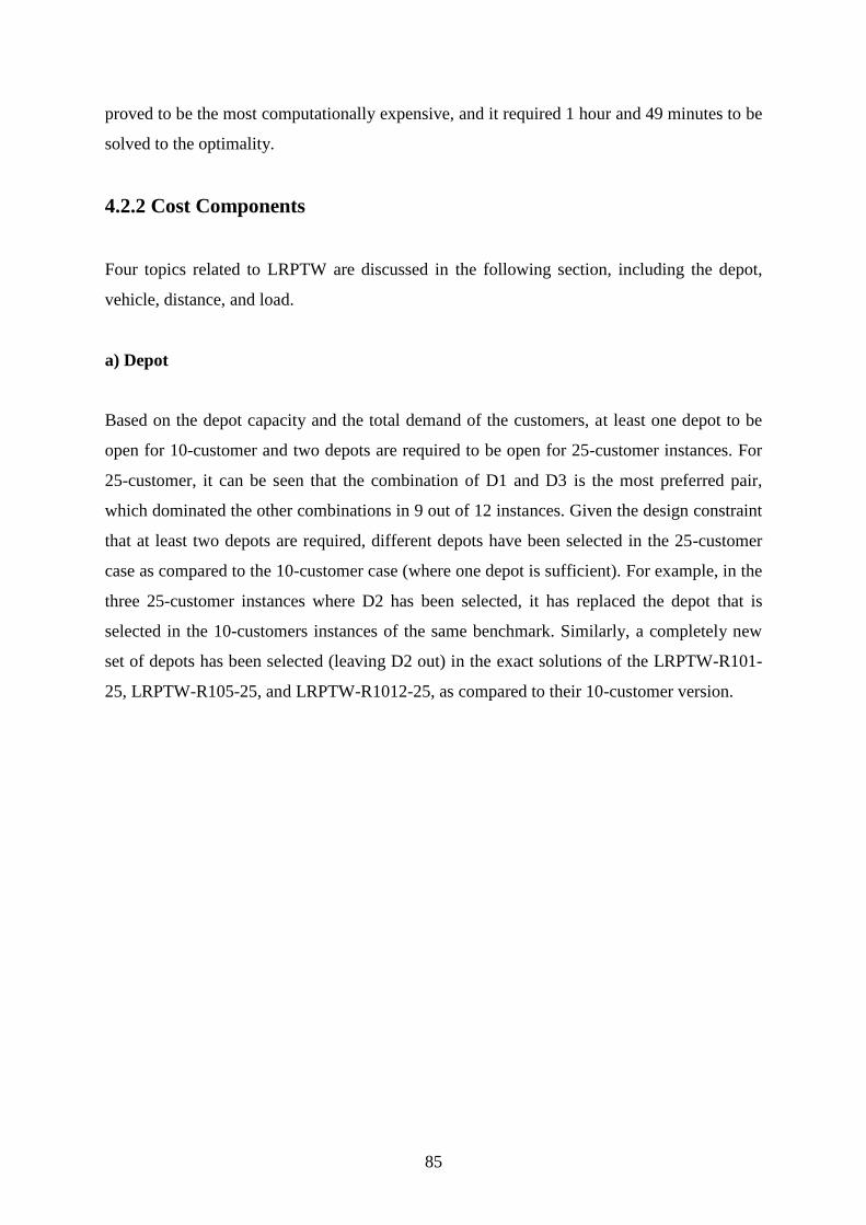
85
proved to be the most computationally expensive, and it required 1 hour and 49 minutes to be
solved to the optimality.
4.2.2 Cost Components
Four topics related to LRPTW are discussed in the following section, including the depot,
vehicle, distance, and load.
a) Depot
Based on the depot capacity and the total demand of the customers, at least one depot to be
open for 10-customer and two depots are required to be open for 25-customer instances. For
25-customer, it can be seen that the combination of D1 and D3 is the most preferred pair,
which dominated the other combinations in 9 out of 12 instances. Given the design constraint
that at least two depots are required, different depots have been selected in the 25-customer
case as compared to the 10-customer case (where one depot is sufficient). For example, in the
three 25-customer instances where D2 has been selected, it has replaced the depot that is
selected in the 10-customers instances of the same benchmark. Similarly, a completely new
set of depots has been selected (leaving D2 out) in the exact solutions of the LRPTW-R101-
25, LRPTW-R105-25, and LRPTW-R1012-25, as compared to their 10-customer version.
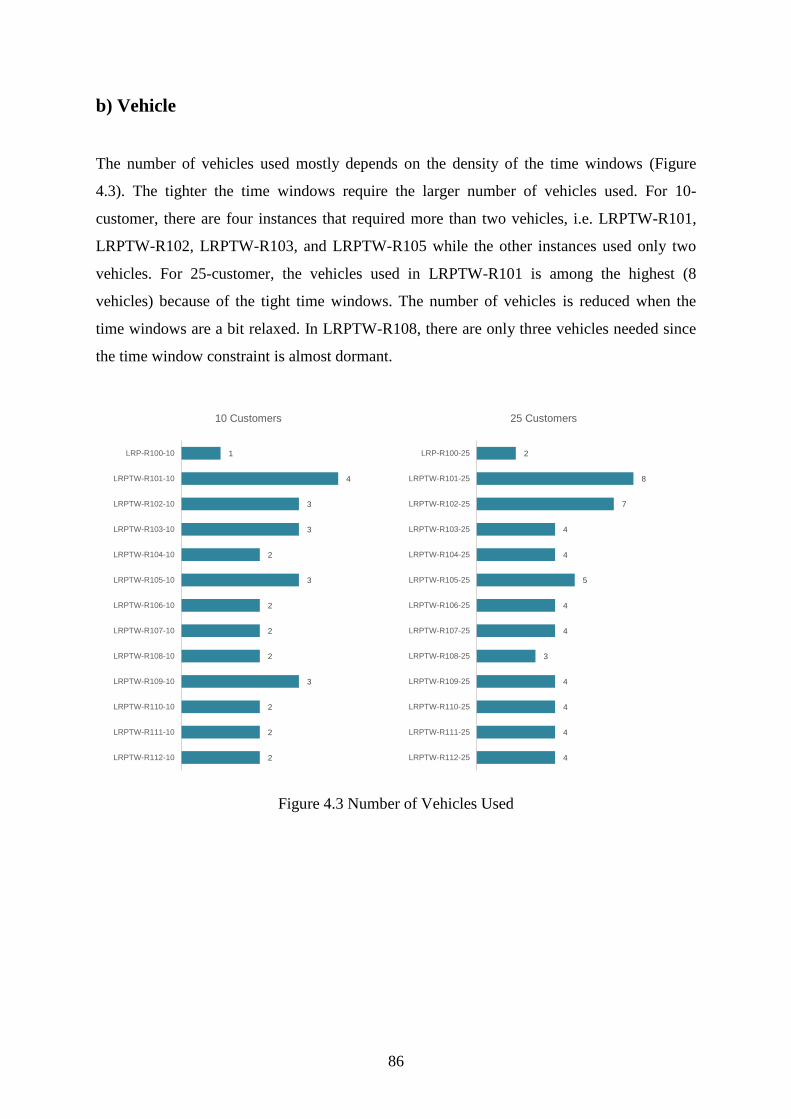
86
b) Vehicle
The number of vehicles used mostly depends on the density of the time windows (Figure
4.3). The tighter the time windows require the larger number of vehicles used. For 10-
customer, there are four instances that required more than two vehicles, i.e. LRPTW-R101,
LRPTW-R102, LRPTW-R103, and LRPTW-R105 while the other instances used only two
vehicles. For 25-customer, the vehicles used in LRPTW-R101 is among the highest (8
vehicles) because of the tight time windows. The number of vehicles is reduced when the
time windows are a bit relaxed. In LRPTW-R108, there are only three vehicles needed since
the time window constraint is almost dormant.
Figure 4.3 Number of Vehicles Used
1
4
3
3
2
3
2
2
2
3
2
2
2
LRP-R100-10
LRPTW-R101-10
LRPTW-R102-10
LRPTW-R103-10
LRPTW-R104-10
LRPTW-R105-10
LRPTW-R106-10
LRPTW-R107-10
LRPTW-R108-10
LRPTW-R109-10
LRPTW-R110-10
LRPTW-R111-10
LRPTW-R112-10
10 Customers
2
8
7
4
4
5
4
4
3
4
4
4
4
LRP-R100-25
LRPTW-R101-25
LRPTW-R102-25
LRPTW-R103-25
LRPTW-R104-25
LRPTW-R105-25
LRPTW-R106-25
LRPTW-R107-25
LRPTW-R108-25
LRPTW-R109-25
LRPTW-R110-25
LRPTW-R111-25
LRPTW-R112-25
25 Customers
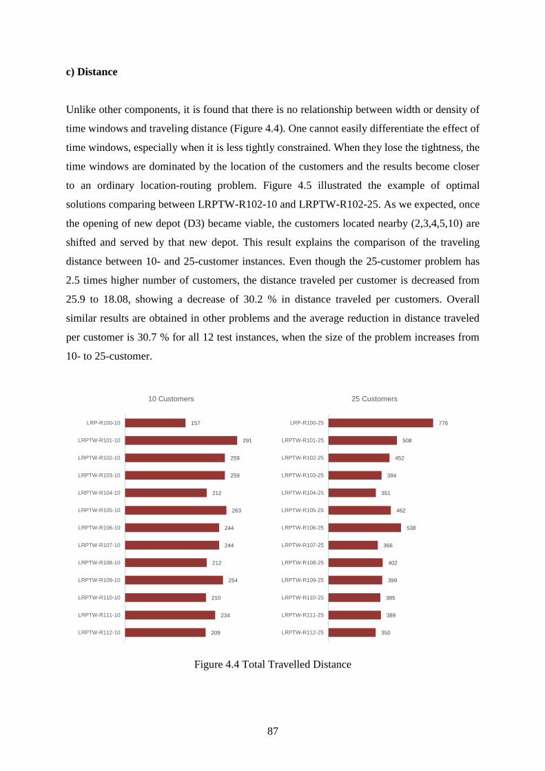
87
c) Distance
Unlike other components, it is found that there is no relationship between width or density of
time windows and traveling distance (Figure 4.4). One cannot easily differentiate the effect of
time windows, especially when it is less tightly constrained. When they lose the tightness, the
time windows are dominated by the location of the customers and the results become closer
to an ordinary location-routing problem. Figure 4.5 illustrated the example of optimal
solutions comparing between LRPTW-R102-10 and LRPTW-R102-25. As we expected, once
the opening of new depot (D3) became viable, the customers located nearby (2,3,4,5,10) are
shifted and served by that new depot. This result explains the comparison of the traveling
distance between 10- and 25-customer instances. Even though the 25-customer problem has
2.5 times higher number of customers, the distance traveled per customer is decreased from
25.9 to 18.08, showing a decrease of 30.2 % in distance traveled per customers. Overall
similar results are obtained in other problems and the average reduction in distance traveled
per customer is 30.7 % for all 12 test instances, when the size of the problem increases from
10- to 25-customer.
Figure 4.4 Total Travelled Distance
157
291
259
259
212
263
244
244
212
254
210
234
209
LRP-R100-10
LRPTW-R101-10
LRPTW-R102-10
LRPTW-R103-10
LRPTW-R104-10
LRPTW-R105-10
LRPTW-R106-10
LRPTW-R107-10
LRPTW-R108-10
LRPTW-R109-10
LRPTW-R110-10
LRPTW-R111-10
LRPTW-R112-10
10 Customers
776
508
452
394
351
462
538
366
402
399
385
389
350
LRP-R100-25
LRPTW-R101-25
LRPTW-R102-25
LRPTW-R103-25
LRPTW-R104-25
LRPTW-R105-25
LRPTW-R106-25
LRPTW-R107-25
LRPTW-R108-25
LRPTW-R109-25
LRPTW-R110-25
LRPTW-R111-25
LRPTW-R112-25
25 Customers
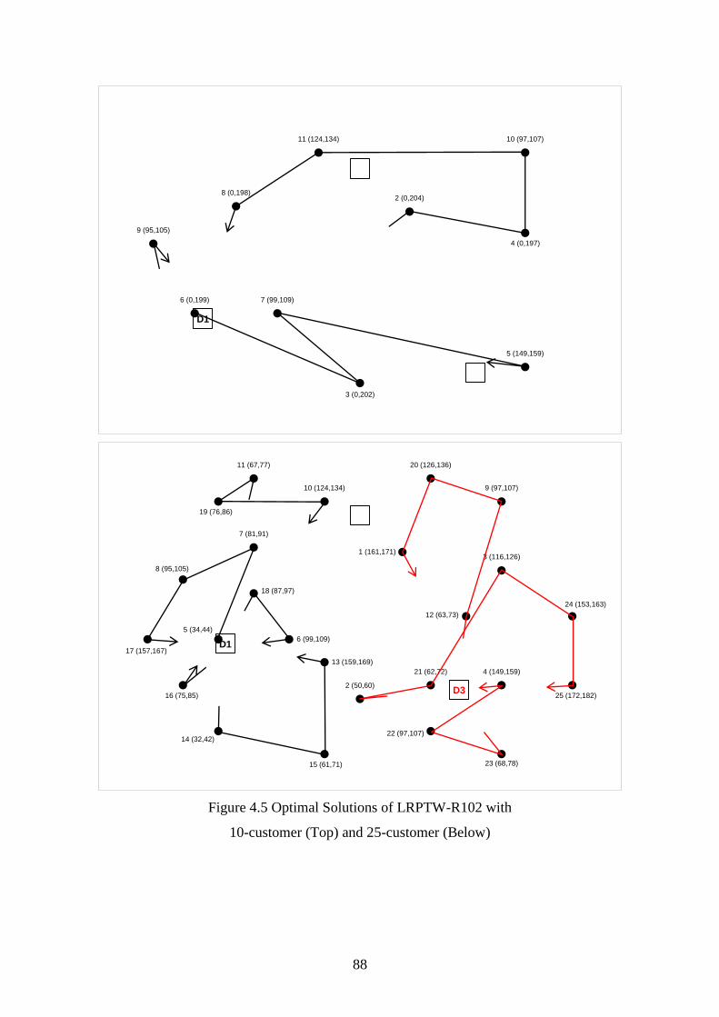
88
Figure 4.5 Optimal Solutions of LRPTW-R102 with
10-customer (Top) and 25-customer (Below)
2 (0,204)
3 (0,202)
4 (0,197)
5 (149,159)
6 (0,199) 7 (99,109)
8 (0,198)
9 (95,105)
10 (97,107)11 (124,134)
D1
D2
D3
1 (161,171)
2 (50,60)
3 (116,126)
4 (149,159)
5 (34,44)
6 (99,109)
7 (81,91)
8 (95,105)
9 (97,107)10 (124,134)
11 (67,77)
12 (63,73)
13 (159,169)
14 (32,42)
15 (61,71)
16 (75,85)
17 (157,167)
18 (87,97)
19 (76,86)
20 (126,136)
21 (62,72)
22 (97,107)
23 (68,78)
24 (153,163)
25 (172,182)
D1
D2
D3
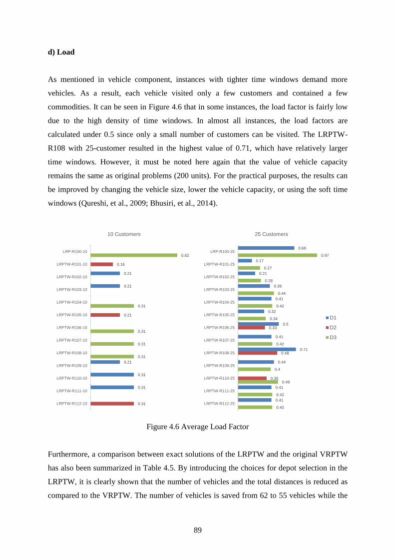
89
d) Load
As mentioned in vehicle component, instances with tighter time windows demand more
vehicles. As a result, each vehicle visited only a few customers and contained a few
commodities. It can be seen in Figure 4.6 that in some instances, the load factor is fairly low
due to the high density of time windows. In almost all instances, the load factors are
calculated under 0.5 since only a small number of customers can be visited. The LRPTW-
R108 with 25-customer resulted in the highest value of 0.71, which have relatively larger
time windows. However, it must be noted here again that the value of vehicle capacity
remains the same as original problems (200 units). For the practical purposes, the results can
be improved by changing the vehicle size, lower the vehicle capacity, or using the soft time
windows (Qureshi, et al., 2009; Bhusiri, et al., 2014).
Figure 4.6 Average Load Factor
Furthermore, a comparison between exact solutions of the LRPTW and the original VRPTW
has also been summarized in Table 4.5. By introducing the choices for depot selection in the
LRPTW, it is clearly shown that the number of vehicles and the total distances is reduced as
compared to the VRPTW. The number of vehicles is saved from 62 to 55 vehicles while the
0.21
0.21
0.21
0.31
0.31
0.16
0.21
0.31
0.62
0.31
0.31
0.31
0.31
LRP-R100-10
LRPTW-R101-10
LRPTW-R102-10
LRPTW-R103-10
LRPTW-R104-10
LRPTW-R105-10
LRPTW-R106-10
LRPTW-R107-10
LRPTW-R108-10
LRPTW-R109-10
LRPTW-R110-10
LRPTW-R111-10
LRPTW-R112-10
10 Customers
0.69
0.17
0.21
0.39
0.41
0.32
0.5
0.41
0.71
0.44
0.41
0.41
0.33
0.48
0.35
0.97
0.27
0.28
0.44
0.42
0.34
0.42
0.4
0.49
0.42
0.42
LRP-R100-25
LRPTW-R101-25
LRPTW-R102-25
LRPTW-R103-25
LRPTW-R104-25
LRPTW-R105-25
LRPTW-R106-25
LRPTW-R107-25
LRPTW-R108-25
LRPTW-R109-25
LRPTW-R110-25
LRPTW-R111-25
LRPTW-R112-25
25 Customers
D1
D2
D3

90
total distance decreased from 5,477 to 4,996 units. Although it can be argued that additional
depots in LRPTW costs more than savings in the distance traveled and number of vehicles,
however, in long terms, these savings may easily subsidize the additional depot costs. This
comparison clearly shows the advantage of simultaneously optimizing the mathematical
problem set at both strategic and operational levels (i.e. in the form of the LRPTW) as
compared to the classic VRPTW.
Table 4.5 Comparison of the Results between LRPTW and Original VRPTW of 25-customer
Problems
Instance
Number of Vehicles
LRPTW VRPTW Difference
D1 D2 D3 Total
R101-25 5 - 3 8 8 0
R102-25 4 - 3 7 7 0
R103-25 2 - 2 4 5 -1
R104-25 2 - 2 4 4 0
R105-25 3 - 2 5 6 -1
R106-25 2 2 - 4 5 -1
R107-25 2 - 2 4 4 0
R108-25 1 2 - 3 4 -1
R109-25 2 - 2 4 5 -1
R110-25 - 2 2 4 5 -1
R111-25 2 - 2 4 5 -1
R112-25 2 - 2 4 4 0
Total 55 62 -7
Table 4.5 (Cont.) Comparison of the Results between LRPTW and Original VRPTW of 25-
customer Problems
Instance
Total Distance
LRPTW VRPTW
%
Different D1 D2 D3 Total
R101-25 268 - 240 508 608 -16%
R102-25 213 - 239 452 540 -16%
R103-25 169 - 225 394 449 -12%
R104-25 161 - 190 351 412 -15%
R105-25 297 - 165 462 524 -12%
R106-25 250 288 - 538 460 17%
R107-25 170 - 196 366 418 -12%
R108-25 115 287 - 402 393 2%
R109-25 198 - 201 399 436 -8%
R110-25 - 175 210 385 424 -9%
R111-25 185 - 204 389 424 -8%
R112-25 159 - 191 350 389 -10%
Total 4,996 5,477 -9%
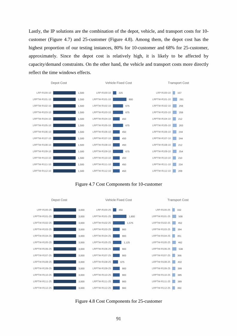
91
Lastly, the IP solutions are the combination of the depot, vehicle, and transport costs for 10-
customer (Figure 4.7) and 25-customer (Figure 4.8). Among them, the depot cost has the
highest proportion of our testing instances, 80% for 10-customer and 68% for 25-customer,
approximately. Since the depot cost is relatively high, it is likely to be affected by
capacity/demand constraints. On the other hand, the vehicle and transport costs more directly
reflect the time windows effects.
Figure 4.7 Cost Components for 10-customer
Figure 4.8 Cost Components for 25-customer
1,500
1,500
1,500
1,500
1,500
1,500
1,500
1,500
1,500
1,500
1,500
1,500
1,500
LRP-R100-10
LRPTW-R101-10
LRPTW-R102-10
LRPTW-R103-10
LRPTW-R104-10
LRPTW-R105-10
LRPTW-R106-10
LRPTW-R107-10
LRPTW-R108-10
LRPTW-R109-10
LRPTW-R110-10
LRPTW-R111-10
LRPTW-R112-10
Depot Cost
225
900
675
675
450
675
450
450
450
675
450
450
450
LRP-R100-10
LRPTW-R101-10
LRPTW-R102-10
LRPTW-R103-10
LRPTW-R104-10
LRPTW-R105-10
LRPTW-R106-10
LRPTW-R107-10
LRPTW-R108-10
LRPTW-R109-10
LRPTW-R110-10
LRPTW-R111-10
LRPTW-R112-10
Vehicle Fixed Cost
157
291
259
259
212
263
244
244
212
254
210
234
209
LRP-R100-10
LRPTW-R101-10
LRPTW-R102-10
LRPTW-R103-10
LRPTW-R104-10
LRPTW-R105-10
LRPTW-R106-10
LRPTW-R107-10
LRPTW-R108-10
LRPTW-R109-10
LRPTW-R110-10
LRPTW-R111-10
LRPTW-R112-10
Transport Cost
3,000
3,000
3,000
3,000
3,000
3,000
3,000
3,000
3,000
3,000
3,000
3,000
3,000
LRP-R100-25
LRPTW-R101-25
LRPTW-R102-25
LRPTW-R103-25
LRPTW-R104-25
LRPTW-R105-25
LRPTW-R106-25
LRPTW-R107-25
LRPTW-R108-25
LRPTW-R109-25
LRPTW-R110-25
LRPTW-R111-25
LRPTW-R112-25
Depot Cost
450
1,800
1,575
900
900
1,125
900
900
675
900
900
900
900
LRP-R100-25
LRPTW-R101-25
LRPTW-R102-25
LRPTW-R103-25
LRPTW-R104-25
LRPTW-R105-25
LRPTW-R106-25
LRPTW-R107-25
LRPTW-R108-25
LRPTW-R109-25
LRPTW-R110-25
LRPTW-R111-25
LRPTW-R112-25
Vehicle Fixed Cost
332
508
452
394
351
462
538
366
402
399
385
389
350
LRP-R100-25
LRPTW-R101-25
LRPTW-R102-25
LRPTW-R103-25
LRPTW-R104-25
LRPTW-R105-25
LRPTW-R106-25
LRPTW-R107-25
LRPTW-R108-25
LRPTW-R109-25
LRPTW-R110-25
LRPTW-R111-25
LRPTW-R112-25
Transport Cost

92
References
Akca, Z., Berger, R. T. & Ralphs, T. K., 2008. Modeling and Solving Location Routing and
Scheduling Problems, Pennsylvania: COR@L Lab, Lehigh University.
Bhusiri, N., Qureshi, A. G. & Taniguchi, E., 2014. The trade-off between fixed vehicle costs
and time-dependent arrival penalties in a routing problem. Transportation Research Part
E: Logistics and Transportation Review, Volume 62, pp. 1-22.
Kaufman, L. & Rousseeuw, P. J., 1987. Clustering by means of medoids. In: Y. Dodge, ed.
Statistical Data Analysis Based on the L1 Norm. Amsterdam: North-Holland, p. 405–416.
Prins, C. et al., 2007. Solving the capacitated location-routing problem by a cooperative
Lagrangean relaxation-granular tabu search heuristic. Transportation Science, 41(4), pp.
470-483.
Prins, C., Prodhon, C. & Wolfler-Calvo, R., 2006. Solving the capacitated location-routing
problem by a GRASP complemented by a learning process and a path relinking. 4OR—A
Quarterly Journal of Operations Research, Volume 4, pp. 221-238.
Qureshi, A., Taniguchi, E. & Yamada, T., 2009. An Exact Solution Approach for Vehicle
Routing and Scheduling Problem with Soft Time Windows. Transportation Research
Part E: Logistics and Transportation Review, 45(6), pp. 960-977.

93
Chapter 5
LRPTW in
Osaka Distribution Network
5.1 Introduction
5.2 Methodology
5.3 Results and Discussion
References

94
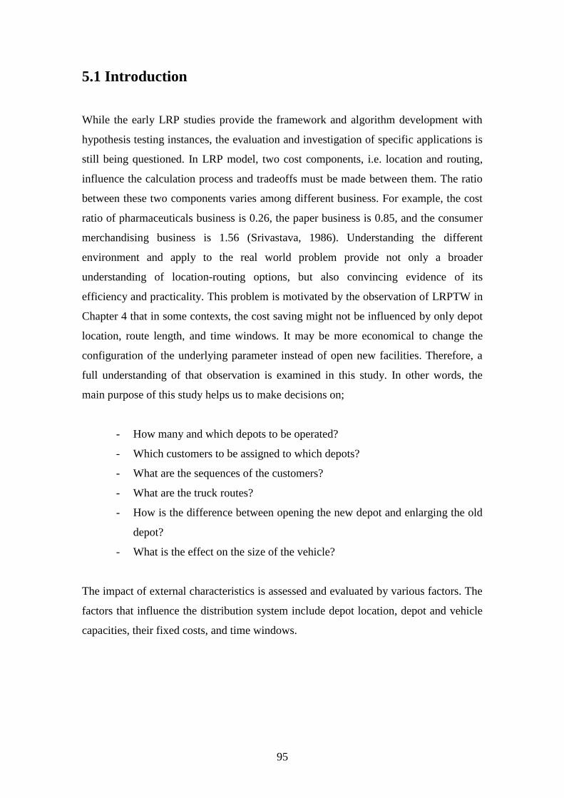
95
5.1 Introduction
While the early LRP studies provide the framework and algorithm development with
hypothesis testing instances, the evaluation and investigation of specific applications is
still being questioned. In LRP model, two cost components, i.e. location and routing,
influence the calculation process and tradeoffs must be made between them. The ratio
between these two components varies among different business. For example, the cost
ratio of pharmaceuticals business is 0.26, the paper business is 0.85, and the consumer
merchandising business is 1.56 (Srivastava, 1986). Understanding the different
environment and apply to the real world problem provide not only a broader
understanding of location-routing options, but also convincing evidence of its
efficiency and practicality. This problem is motivated by the observation of LRPTW in
Chapter 4 that in some contexts, the cost saving might not be influenced by only depot
location, route length, and time windows. It may be more economical to change the
configuration of the underlying parameter instead of open new facilities. Therefore, a
full understanding of that observation is examined in this study. In other words, the
main purpose of this study helps us to make decisions on;
- How many and which depots to be operated?
- Which customers to be assigned to which depots?
- What are the sequences of the customers?
- What are the truck routes?
- How is the difference between opening the new depot and enlarging the old
depot?
- What is the effect on the size of the vehicle?
The impact of external characteristics is assessed and evaluated by various factors. The
factors that influence the distribution system include depot location, depot and vehicle
capacities, their fixed costs, and time windows.
96
5.2 Methodology
The distribution data from freight carrier have been tested with the branch-and-price
algorithm to evaluate the cost structure and environmental impact on the location-
routing problem. The selected logistic company provides a variety of services including
warehousing, storage and inventory management, and door to door delivery. Fresh
food, medical specimens, and large items are among the commodities to be delivered
on the daily basis (Teo, et al., 2015). The transportation information is collected by the
global positioning system (GPS) during the real time operation. It provides the
customers’ location, delivery routes, and traveling speed. Moreover, the additional
travel times on the road networks, which have never been collected by the GPS are
collected from the traffic census data from Osaka city (MLIT, 2010). Figure 5.1 and 5.2
shows the location of depots and selected customers in the city of Osaka. The depots
are located at Toyonaka-shi, Minato-ku, and Nishinari-ku. The travel times between
depot to the customer and customer to the customer are converted and calculated the
shortest path using Dijkstra’s algorithm. It must be noted here that the carrier
specifically classifies some private information. Therefore, the logistics data including
customers’ demand are randomly hypothetical. The time window width (bi - ai) and
service time are constantly set equal to 30 and 10 minutes, respectively.
Three influence factors to be evaluated in the test instance are depot and vehicle
configuration, i.e. location, size, and cost. Three sizes of depots and vehicles, i.e. small,
medium, and large, make a combination of nine scenarios. It is quite obvious that the
size and cost are interdependence since the larger depot space is costly. However, the
warehousing cost varies by their locations. We estimated the depots’ cost (fm) and
capacity (Qm) based on the data available from commercial real estate service firm
(JLRE, 2015). For the vehicle, the capacity (q) of 1,340 kg, 2 ton, and 3 ton trucks
represent the small, medium, large vehicles. The vehicle fixed costs (cmj) are 5,209,
7,441, and 10,418 yen per vehicle, respectively. The vehicle operating cost (cij) is 14.02
yen per minute (Qureshi, et al., 2014; Toyota, 2015). The morning and afternoon
services are assumed to be exactly the same. Table 5.1 and 5.2 show the parameters
used in our calculation.
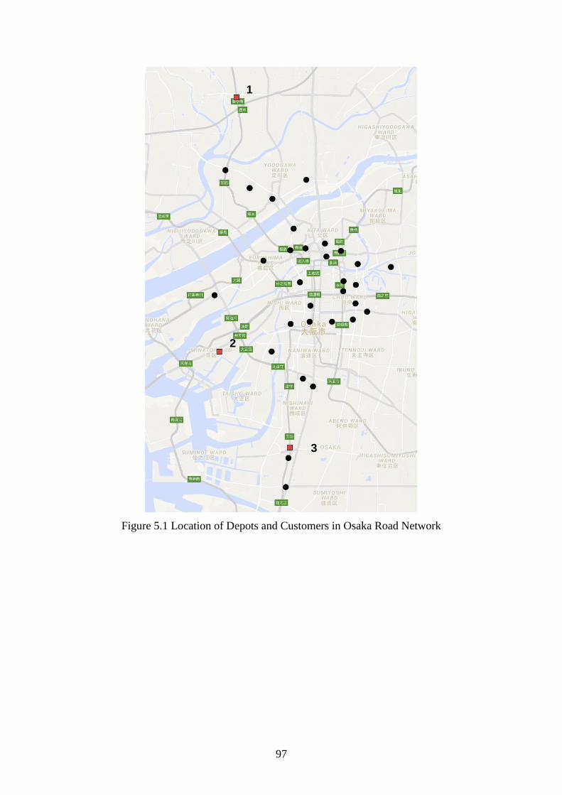
97
Figure 5.1 Location of Depots and Customers in Osaka Road Network
1
2
3
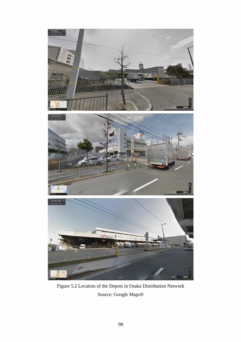
98
Figure 5.2 Location of the Depots in Osaka Distribution Network
Source: Google Maps®
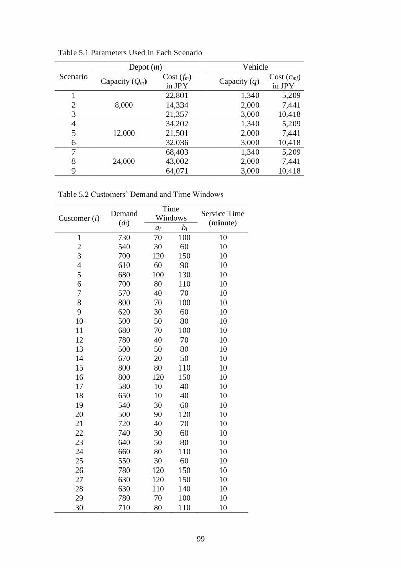
99
Table 5.1 Parameters Used in Each Scenario
Scenario
Depot (m) Vehicle
Capacity (Qm) Cost (fm)
in JPY
Capacity (q)
Cost (cmj)
in JPY
1
8,000
22,801 1,340 5,209
2 14,334 2,000 7,441
3 21,357 3,000 10,418
4
12,000
34,202 1,340 5,209
5 21,501 2,000 7,441
6 32,036 3,000 10,418
7
24,000
68,403 1,340 5,209
8 43,002 2,000 7,441
9 64,071 3,000 10,418
Table 5.2 Customers’ Demand and Time Windows
Customer (i) Demand
(di)
Time
Windows Service Time
(minute) ai bi
1 730 70 100 10
2 540 30 60 10
3 700 120 150 10
4 610 60 90 10
5 680 100 130 10
6 700 80 110 10
7 570 40 70 10
8 800 70 100 10
9 620 30 60 10
10 500 50 80 10
11 680 70 100 10
12 780 40 70 10
13 500 50 80 10
14 670 20 50 10
15 800 80 110 10
16 800 120 150 10
17 580 10 40 10
18 650 10 40 10
19 540 30 60 10
20 500 90 120 10
21 720 40 70 10
22 740 30 60 10
23 640 50 80 10
24 660 80 110 10
25 550 30 60 10
26 780 120 150 10
27 630 120 150 10
28 630 110 140 10
29 780 70 100 10
30 710 80 110 10
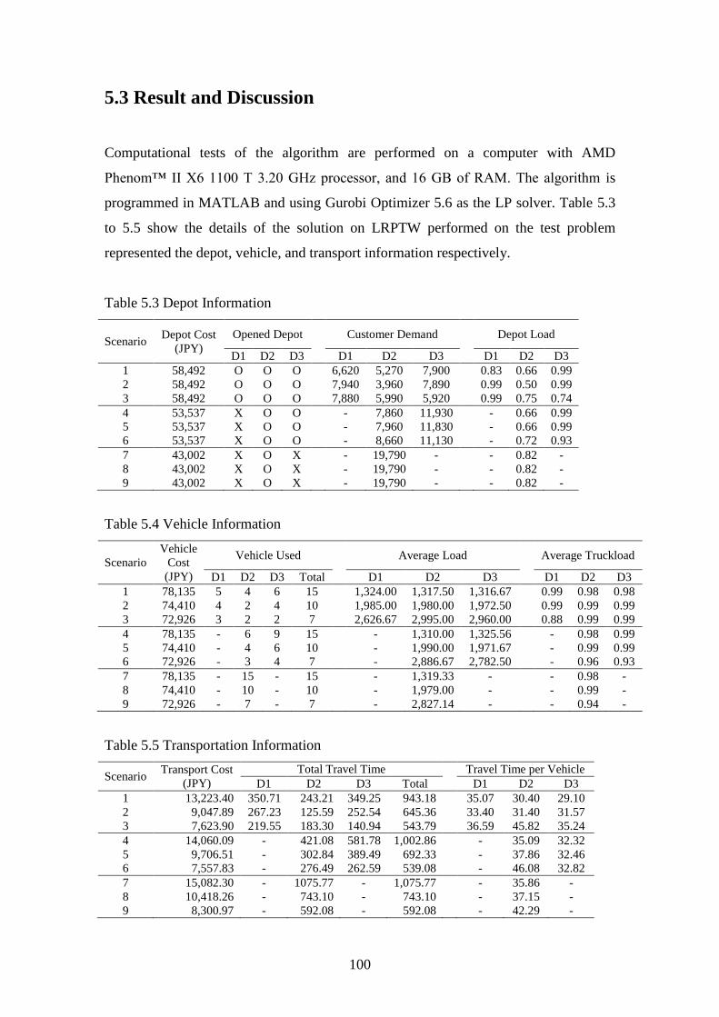
100
5.3 Result and Discussion
Computational tests of the algorithm are performed on a computer with AMD
Phenom™ II X6 1100 T 3.20 GHz processor, and 16 GB of RAM. The algorithm is
programmed in MATLAB and using Gurobi Optimizer 5.6 as the LP solver. Table 5.3
to 5.5 show the details of the solution on LRPTW performed on the test problem
represented the depot, vehicle, and transport information respectively.
Table 5.3 Depot Information
Scenario Depot Cost
(JPY)
Opened Depot
Customer Demand
Depot Load
D1 D2 D3 D1 D2 D3 D1 D2 D3
1 58,492 O O O 6,620 5,270 7,900 0.83 0.66 0.99
2 58,492 O O O 7,940 3,960 7,890 0.99 0.50 0.99
3 58,492 O O O 7,880 5,990 5,920 0.99 0.75 0.74
4 53,537 X O O - 7,860 11,930 - 0.66 0.99
5 53,537 X O O - 7,960 11,830 - 0.66 0.99
6 53,537 X O O - 8,660 11,130 - 0.72 0.93
7 43,002 X O X - 19,790 - - 0.82 -
8 43,002 X O X - 19,790 - - 0.82 -
9 43,002 X O X - 19,790 - - 0.82 -
Table 5.4 Vehicle Information
Scenario
Vehicle
Cost
(JPY)
Vehicle Used
Average Load
Average Truckload
D1 D2 D3 Total D1 D2 D3 D1 D2 D3
1 78,135 5 4 6 15 1,324.00 1,317.50 1,316.67 0.99 0.98 0.98
2 74,410 4 2 4 10 1,985.00 1,980.00 1,972.50 0.99 0.99 0.99
3 72,926 3 2 2 7 2,626.67 2,995.00 2,960.00 0.88 0.99 0.99
4 78,135 - 6 9 15 - 1,310.00 1,325.56 - 0.98 0.99
5 74,410 - 4 6 10 - 1,990.00 1,971.67 - 0.99 0.99
6 72,926 - 3 4 7 - 2,886.67 2,782.50 - 0.96 0.93
7 78,135 - 15 - 15 - 1,319.33 - - 0.98 -
8 74,410 - 10 - 10 - 1,979.00 - - 0.99 -
9 72,926 - 7 - 7 - 2,827.14 - - 0.94 -
Table 5.5 Transportation Information
Scenario Transport Cost
(JPY)
Total Travel Time Travel Time per Vehicle
D1 D2 D3 Total D1 D2 D3
1 13,223.40 350.71 243.21 349.25 943.18 35.07 30.40 29.10
2 9,047.89 267.23 125.59 252.54 645.36 33.40 31.40 31.57
3 7,623.90 219.55 183.30 140.94 543.79 36.59 45.82 35.24
4 14,060.09 - 421.08 581.78 1,002.86 - 35.09 32.32
5 9,706.51 - 302.84 389.49 692.33 - 37.86 32.46
6 7,557.83 - 276.49 262.59 539.08 - 46.08 32.82
7 15,082.30 - 1075.77 - 1,075.77 - 35.86 -
8 10,418.26 - 743.10 - 743.10 - 37.15 -
9 8,300.97 - 592.08 - 592.08 - 42.29 -
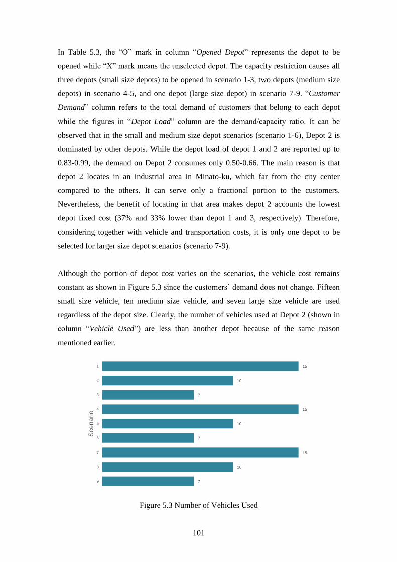
101
In Table 5.3, the “O” mark in column “Opened Depot” represents the depot to be
opened while “X” mark means the unselected depot. The capacity restriction causes all
three depots (small size depots) to be opened in scenario 1-3, two depots (medium size
depots) in scenario 4-5, and one depot (large size depot) in scenario 7-9. “Customer
Demand” column refers to the total demand of customers that belong to each depot
while the figures in “Depot Load” column are the demand/capacity ratio. It can be
observed that in the small and medium size depot scenarios (scenario 1-6), Depot 2 is
dominated by other depots. While the depot load of depot 1 and 2 are reported up to
0.83-0.99, the demand on Depot 2 consumes only 0.50-0.66. The main reason is that
depot 2 locates in an industrial area in Minato-ku, which far from the city center
compared to the others. It can serve only a fractional portion to the customers.
Nevertheless, the benefit of locating in that area makes depot 2 accounts the lowest
depot fixed cost (37% and 33% lower than depot 1 and 3, respectively). Therefore,
considering together with vehicle and transportation costs, it is only one depot to be
selected for larger size depot scenarios (scenario 7-9).
Although the portion of depot cost varies on the scenarios, the vehicle cost remains
constant as shown in Figure 5.3 since the customers’ demand does not change. Fifteen
small size vehicle, ten medium size vehicle, and seven large size vehicle are used
regardless of the depot size. Clearly, the number of vehicles used at Depot 2 (shown in
column “Vehicle Used”) are less than another depot because of the same reason
mentioned earlier.
Figure 5.3 Number of Vehicles Used
15
10
7
15
10
7
15
10
7
1
2
3
4
5
6
7
8
9
Scenario
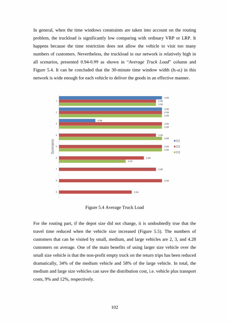
102
In general, when the time windows constraints are taken into account on the routing
problem, the truckload is significantly low comparing with ordinary VRP or LRP. It
happens because the time restriction does not allow the vehicle to visit too many
numbers of customers. Nevertheless, the truckload in our network is relatively high in
all scenarios, presented 0.94-0.99 as shown in “Average Truck Load” column and
Figure 5.4. It can be concluded that the 30-minute time window width (bi-ai) in this
network is wide enough for each vehicle to deliver the goods in an effective manner.
Figure 5.4 Average Truck Load
For the routing part, if the depot size did not change, it is undoubtedly true that the
travel time reduced when the vehicle size increased (Figure 5.5). The numbers of
customers that can be visited by small, medium, and large vehicles are 2, 3, and 4.28
customers on average. One of the main benefits of using larger size vehicle over the
small size vehicle is that the non-profit empty truck on the return trips has been reduced
dramatically, 34% of the medium vehicle and 58% of the large vehicle. In total, the
medium and large size vehicles can save the distribution cost, i.e. vehicle plus transport
costs, 9% and 12%, respectively.
0.99
0.99
0.88
0.98
0.99
0.99
0.98
0.99
0.96
0.98
0.99
0.94
0.98
0.99
0.99
0.99
0.99
0.93
1
2
3
4
5
6
7
8
9
Scenario D1
D2
D3
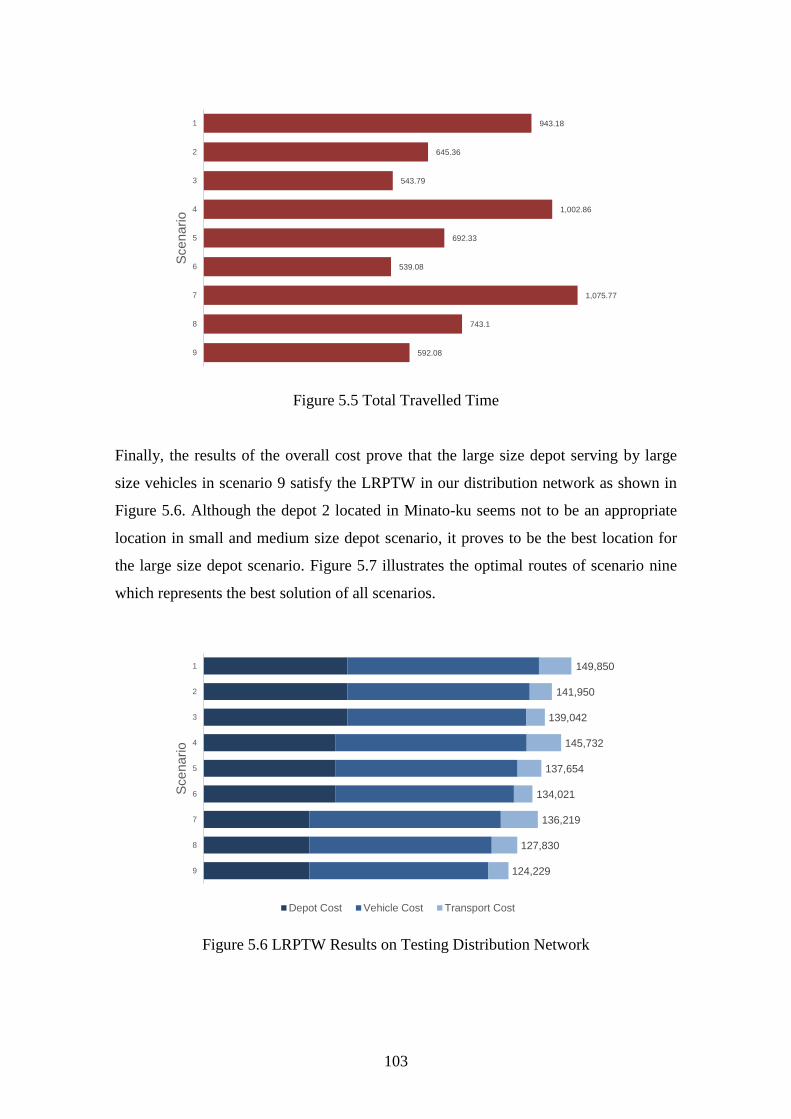
103
Figure 5.5 Total Travelled Time
Finally, the results of the overall cost prove that the large size depot serving by large
size vehicles in scenario 9 satisfy the LRPTW in our distribution network as shown in
Figure 5.6. Although the depot 2 located in Minato-ku seems not to be an appropriate
location in small and medium size depot scenario, it proves to be the best location for
the large size depot scenario. Figure 5.7 illustrates the optimal routes of scenario nine
which represents the best solution of all scenarios.
Figure 5.6 LRPTW Results on Testing Distribution Network
943.18
645.36
543.79
1,002.86
692.33
539.08
1,075.77
743.1
592.08
1
2
3
4
5
6
7
8
9
Scenario
149,850
141,950
139,042
145,732
137,654
134,021
136,219
127,830
124,229
1
2
3
4
5
6
7
8
9
Scenario
Depot Cost Vehicle Cost Transport Cost
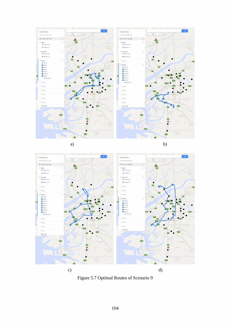
104
a) b)
c) d)
Figure 5.7 Optimal Routes of Scenario 9
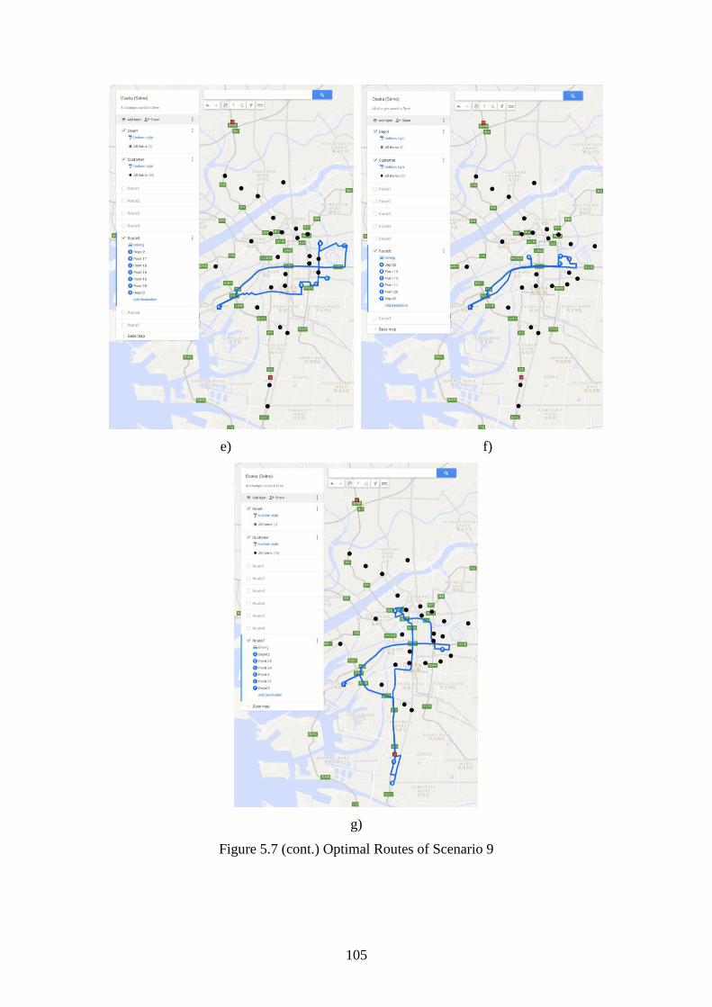
105
e) f)
g)
Figure 5.7 (cont.) Optimal Routes of Scenario 9
106
References
JLRE, 2015. Warehouse for rent/Logistics real estate. [Online] Available at:
http://lw.e-sohko.com/ [Accessed 25 1 2015].
MLIT, 2010. Ministry of Land, Infrastructure, Transport, and Tourism: 2010
nationwide road and street traffic situation investigation. [Online] Available at:
http://www.mlit.go.jp/road/census/h22-1/ [Accessed 20 1 2012].
Nakanishi, H., Matsuo, K. & Black, J., 2013. Transportation planning methodologies
for post-disaster recovery in regional communities: the East Japan Earthquake and
tsunami 2011. Journal of Transport Geography, Volume 31, pp. 181-191.
Ponboon, S., Qureshi, A. G. & Taniguchi, E., 2014. Exact Solution for Location-
Routing Problem with Time Windows using Branch-and-Price Algorithm.
Transportation Research Part E: Logistics and Transportation Review, Volume
(Submitted).
Ponboon, S., Taniguchi, E. & Qureshi, A. G., 2013. Integrated Approach for Location-
Routing Problem using Branch-and-Price Method. Hiroshima, JSCE 47th
Conference on Infrastructure Planning and Management.
Qureshi, A., Taniguchi, E., Thompson, R. & Teo, J., 2014. Application of exact route
optimization for the evaluation of a city logistics truck ban scheme. International
Journal of Urban Sciences, 18(2), pp. 117-132.
Srivastava, R., 1986. Algorithms for solving the location-routing problem, Columbus,
Ohio: PhD dissertation, The Ohio State University.
Taniguchi, E. & Thompson, R. G., 2013. Humanitarian Logistics in the Great Tohoku
Disasters 2011. In: V. Zeimpekis, S. Ichoua & I. Minis, eds. Humanitarian and
Relief Logistics. New York: Springer, pp. 207-218.
Teo, J. et al., 2015. Towards a safer and healthier urbanization by improving land use
footprint of last-mile freight delivery. Washington D.C., 94th Transportation
Research Board Annual Meeting Compendium of Papers.
Toyota Motor Corporation, 2015. Toyota Rent a Car. [Online] Available at:
https://rent.toyota.co.jp/eng/index.html [Accessed 11 05 2015].
Toyota, 2015. Rate and Car Model List. [Online] Available at:
https://rent.toyota.co.jp/en/rental/main09.html [Accessed 25 1 2015].
107
Chapter 6
LRPTW in
Ishinomaki Humanitarian Logistics
6.1 Introduction
6.2 Scenarios
6.3 Tabu Search Heuristic
6.3.1 Route Construction
6.3.2 Route Improvement
6.3.3 Model Validation
6.4 Results and Discussions
References

108
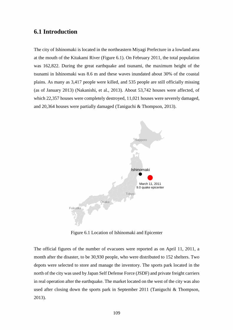
109
6.1 Introduction
The city of Ishinomaki is located in the northeastern Miyagi Prefecture in a lowland area
at the mouth of the Kitakami River (Figure 6.1). On February 2011, the total population
was 162,822. During the great earthquake and tsunami, the maximum height of the
tsunami in Ishinomaki was 8.6 m and these waves inundated about 30% of the coastal
plains. As many as 3,417 people were killed, and 535 people are still officially missing
(as of January 2013) (Nakanishi, et al., 2013). About 53,742 houses were affected, of
which 22,357 houses were completely destroyed, 11,021 houses were severely damaged,
and 20,364 houses were partially damaged (Taniguchi & Thompson, 2013).
Figure 6.1 Location of Ishinomaki and Epicenter
The official figures of the number of evacuees were reported as on April 11, 2011, a
month after the disaster, to be 30,930 people, who were distributed to 152 shelters. Two
depots were selected to store and manage the inventory. The sports park located in the
north of the city was used by Japan Self Defense Force (JSDF) and private freight carriers
in real operation after the earthquake. The market located on the west of the city was also
used after closing down the sports park in September 2011 (Taniguchi & Thompson,
2013).
Ishinomaki
March 11, 2011 9.0 quake epicenter
Tokyo
Osaka
Sapporo
Fukuoka
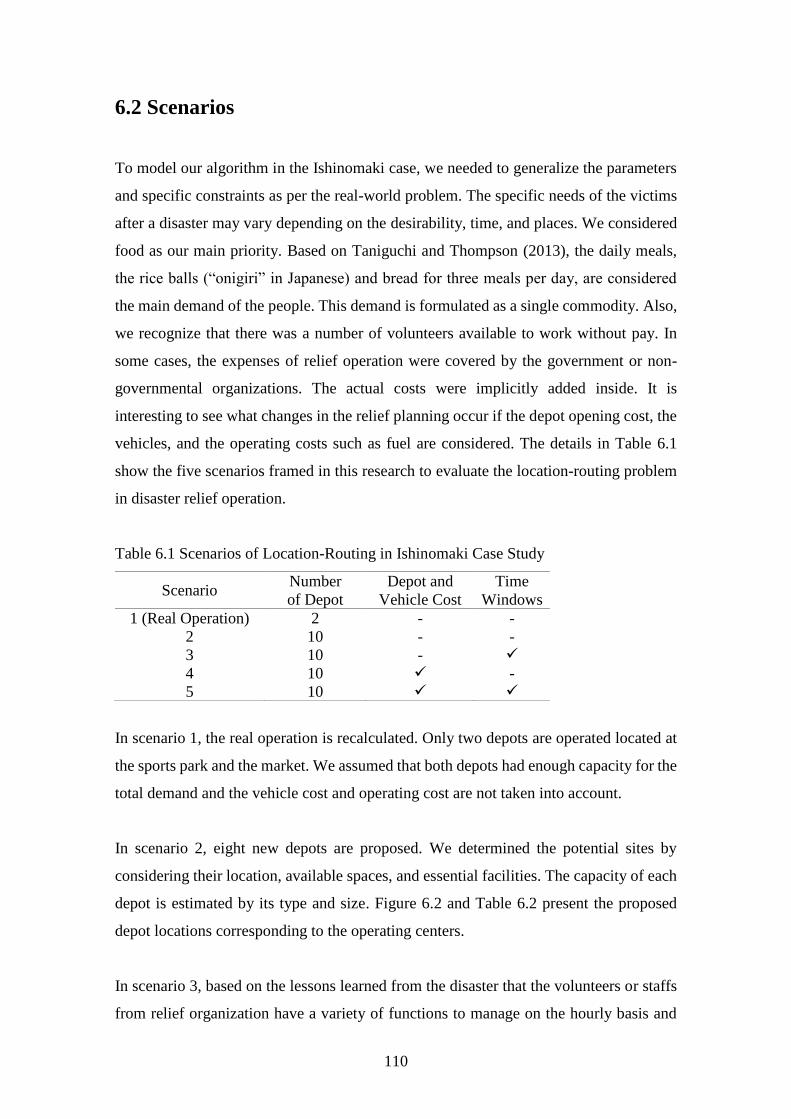
110
6.2 Scenarios
To model our algorithm in the Ishinomaki case, we needed to generalize the parameters
and specific constraints as per the real-world problem. The specific needs of the victims
after a disaster may vary depending on the desirability, time, and places. We considered
food as our main priority. Based on Taniguchi and Thompson (2013), the daily meals,
the rice balls (“onigiri” in Japanese) and bread for three meals per day, are considered
the main demand of the people. This demand is formulated as a single commodity. Also,
we recognize that there was a number of volunteers available to work without pay. In
some cases, the expenses of relief operation were covered by the government or non-
governmental organizations. The actual costs were implicitly added inside. It is
interesting to see what changes in the relief planning occur if the depot opening cost, the
vehicles, and the operating costs such as fuel are considered. The details in Table 6.1
show the five scenarios framed in this research to evaluate the location-routing problem
in disaster relief operation.
Table 6.1 Scenarios of Location-Routing in Ishinomaki Case Study
Scenario Number
of Depot
Depot and
Vehicle Cost
Time
Windows
1 (Real Operation) 2 - -
2 10 - -
3 10 -
4 10 -
5 10
In scenario 1, the real operation is recalculated. Only two depots are operated located at
the sports park and the market. We assumed that both depots had enough capacity for the
total demand and the vehicle cost and operating cost are not taken into account.
In scenario 2, eight new depots are proposed. We determined the potential sites by
considering their location, available spaces, and essential facilities. The capacity of each
depot is estimated by its type and size. Figure 6.2 and Table 6.2 present the proposed
depot locations corresponding to the operating centers.
In scenario 3, based on the lessons learned from the disaster that the volunteers or staffs
from relief organization have a variety of functions to manage on the hourly basis and
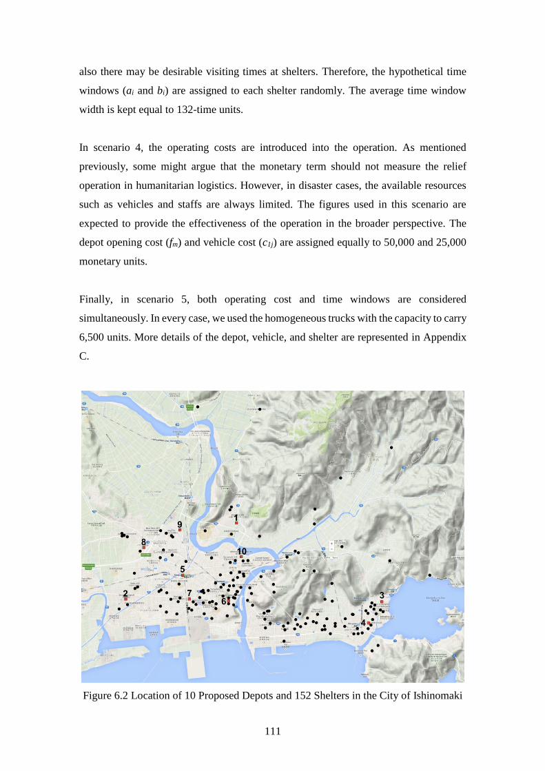
111
also there may be desirable visiting times at shelters. Therefore, the hypothetical time
windows (ai and bi) are assigned to each shelter randomly. The average time window
width is kept equal to 132-time units.
In scenario 4, the operating costs are introduced into the operation. As mentioned
previously, some might argue that the monetary term should not measure the relief
operation in humanitarian logistics. However, in disaster cases, the available resources
such as vehicles and staffs are always limited. The figures used in this scenario are
expected to provide the effectiveness of the operation in the broader perspective. The
depot opening cost (fm) and vehicle cost (c1j) are assigned equally to 50,000 and 25,000
monetary units.
Finally, in scenario 5, both operating cost and time windows are considered
simultaneously. In every case, we used the homogeneous trucks with the capacity to carry
6,500 units. More details of the depot, vehicle, and shelter are represented in Appendix
C.
Figure 6.2 Location of 10 Proposed Depots and 152 Shelters in the City of Ishinomaki
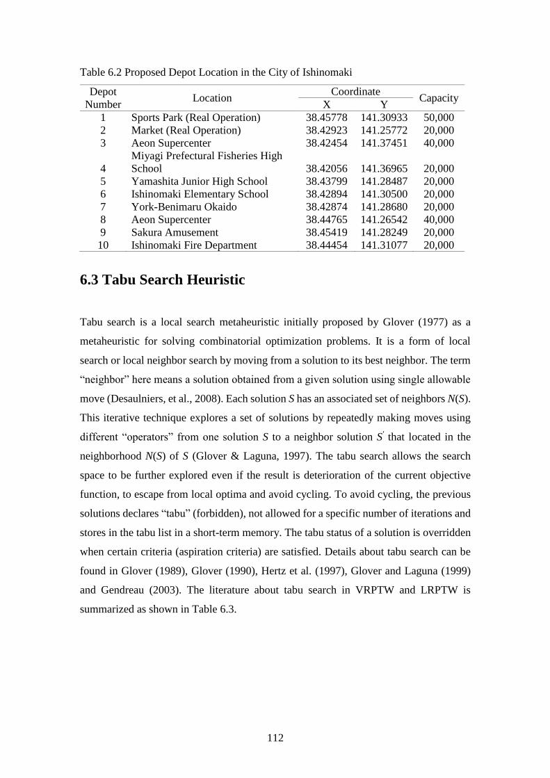
112
Table 6.2 Proposed Depot Location in the City of Ishinomaki
Depot
Number Location
Coordinate Capacity
X Y
1 Sports Park (Real Operation) 38.45778 141.30933 50,000
2 Market (Real Operation) 38.42923 141.25772 20,000
3 Aeon Supercenter 38.42454 141.37451 40,000
4
Miyagi Prefectural Fisheries High
School 38.42056 141.36965 20,000
5 Yamashita Junior High School 38.43799 141.28487 20,000
6 Ishinomaki Elementary School 38.42894 141.30500 20,000
7 York-Benimaru Okaido 38.42874 141.28680 20,000
8 Aeon Supercenter 38.44765 141.26542 40,000
9 Sakura Amusement 38.45419 141.28249 20,000
10 Ishinomaki Fire Department 38.44454 141.31077 20,000
6.3 Tabu Search Heuristic
Tabu search is a local search metaheuristic initially proposed by Glover (1977) as a
metaheuristic for solving combinatorial optimization problems. It is a form of local
search or local neighbor search by moving from a solution to its best neighbor. The term
“neighbor” here means a solution obtained from a given solution using single allowable
move (Desaulniers, et al., 2008). Each solution S has an associated set of neighbors N(S).
This iterative technique explores a set of solutions by repeatedly making moves using
different “operators” from one solution S to a neighbor solution S′ that located in the
neighborhood N(S) of S (Glover & Laguna, 1997). The tabu search allows the search
space to be further explored even if the result is deterioration of the current objective
function, to escape from local optima and avoid cycling. To avoid cycling, the previous
solutions declares “tabu” (forbidden), not allowed for a specific number of iterations and
stores in the tabu list in a short-term memory. The tabu status of a solution is overridden
when certain criteria (aspiration criteria) are satisfied. Details about tabu search can be
found in Glover (1989), Glover (1990), Hertz et al. (1997), Glover and Laguna (1999)
and Gendreau (2003). The literature about tabu search in VRPTW and LRPTW is
summarized as shown in Table 6.3.
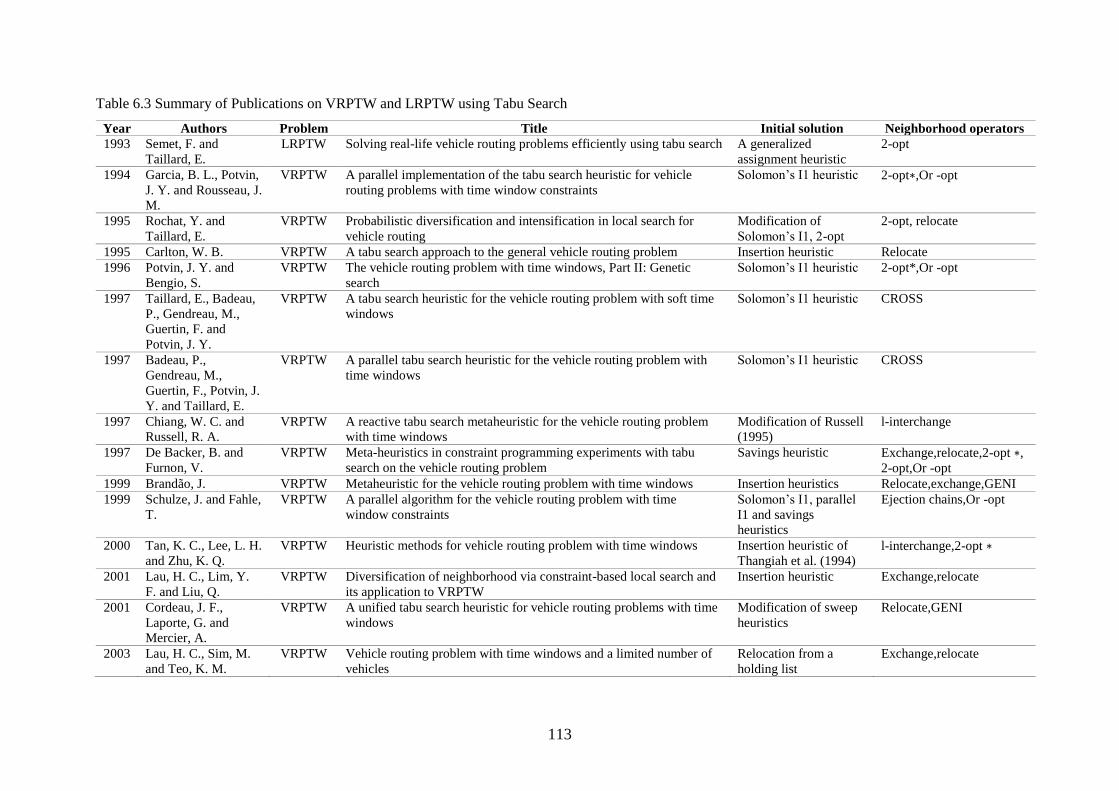
113
Table 6.3 Summary of Publications on VRPTW and LRPTW using Tabu Search
Year Authors Problem Title Initial solution Neighborhood operators
1993 Semet, F. and
Taillard, E.
LRPTW Solving real-life vehicle routing problems efficiently using tabu search A generalized
assignment heuristic
2-opt
1994 Garcia, B. L., Potvin,
J. Y. and Rousseau, J.
M.
VRPTW A parallel implementation of the tabu search heuristic for vehicle
routing problems with time window constraints
Solomon’s I1 heuristic 2-opt∗,Or -opt
1995 Rochat, Y. and
Taillard, E.
VRPTW Probabilistic diversification and intensification in local search for
vehicle routing
Modification of
Solomon’s I1, 2-opt
2-opt, relocate
1995 Carlton, W. B. VRPTW A tabu search approach to the general vehicle routing problem Insertion heuristic Relocate
1996 Potvin, J. Y. and
Bengio, S.
VRPTW The vehicle routing problem with time windows, Part II: Genetic
search
Solomon’s I1 heuristic 2-opt*,Or -opt
1997 Taillard, E., Badeau,
P., Gendreau, M.,
Guertin, F. and
Potvin, J. Y.
VRPTW A tabu search heuristic for the vehicle routing problem with soft time
windows
Solomon’s I1 heuristic CROSS
1997 Badeau, P.,
Gendreau, M.,
Guertin, F., Potvin, J.
Y. and Taillard, E.
VRPTW A parallel tabu search heuristic for the vehicle routing problem with
time windows
Solomon’s I1 heuristic CROSS
1997 Chiang, W. C. and
Russell, R. A.
VRPTW A reactive tabu search metaheuristic for the vehicle routing problem
with time windows
Modification of Russell
(1995)
l-interchange
1997 De Backer, B. and
Furnon, V.
VRPTW Meta-heuristics in constraint programming experiments with tabu
search on the vehicle routing problem
Savings heuristic Exchange,relocate,2-opt ∗,
2-opt,Or -opt
1999 Brandão, J. VRPTW Metaheuristic for the vehicle routing problem with time windows Insertion heuristics Relocate,exchange,GENI
1999 Schulze, J. and Fahle,
T.
VRPTW A parallel algorithm for the vehicle routing problem with time
window constraints
Solomon’s I1, parallel
I1 and savings
heuristics
Ejection chains,Or -opt
2000 Tan, K. C., Lee, L. H.
and Zhu, K. Q.
VRPTW Heuristic methods for vehicle routing problem with time windows Insertion heuristic of
Thangiah et al. (1994) l-interchange,2-opt ∗
2001 Lau, H. C., Lim, Y.
F. and Liu, Q.
VRPTW Diversification of neighborhood via constraint-based local search and
its application to VRPTW
Insertion heuristic Exchange,relocate
2001 Cordeau, J. F.,
Laporte, G. and
Mercier, A.
VRPTW A unified tabu search heuristic for vehicle routing problems with time
windows
Modification of sweep
heuristics
Relocate,GENI
2003 Lau, H. C., Sim, M.
and Teo, K. M.
VRPTW Vehicle routing problem with time windows and a limited number of
vehicles
Relocation from a
holding list
Exchange,relocate

114
Year Authors Problem Title Initial solution Neighborhood operators
2006 Burks, R. LRPTW An Adaptive Tabu Search Heuristic for the Location Routing Pickup
and Delivery Problem with Time Windows with a Theater
Distribution Application
Distance based greedy
heuristic
Cycle swap, route insert,
reallocation insert, and
extraction insert
2009 Schittekat, P. and
Sorensen, K.
LRPTW Or practice - supporting 3PL decisions in the automotive industry by
generating diverse solutions to a large-scale location-routing problem
Random chosen Add, drop, swap
2011 Gündüz, H. I. LRPTW The Single-Stage Location-Routing Problem with Time Windows Savings heuristic 2-opt, 2-opt∗, Or-opt,
relocate, exchange, and
cross-exchange

115
Our tabu search algorithm consists of two parts. It includes route construction and route
improvement.
6.3.1 Route Construction
The route construction selects nodes sequentially until a feasible solution is created. Nodes are
selected based on the cost minimization criterion, and meet vehicle capacity and time window
constraints (Bräysy & Gendreau, 2005).
To build an initial solution, three sub-stages including depot selection, customer allocation, and
route construction are examined in this section. Since the depot cost is relatively high
comparing with transportation cost, the depot(s) mM that has a lowest depot cost is/are
selected as an initial opendepot regardless of its location. At this point, two or more depots
might be assigned whenever the customers’ demand does not exceed the open depots’ capacity.
Next, each customer cC is assigned to the nearest open depot. If the total demand exceeds
depot capacity, the customer located near to another depot will be moved to that particular
depot. Finally, the routes are constructed using insertion heuristics. An intuitive approach to
the LRPTW is to assign all customers as unroute. Then, the tour is build by inserting the
remaining “cheapest insertion” customers one after another with minimizing the cost to route
(r) until all nodes have been inserted. At each insertion, new route r is initially constructed if
the vehicle capacity and time windows constraints are violated. The algorithm ends when no
customer in unroute remains.
The fundamental of insertion heuristics is to start with a tour of a subset of all customers, and
then extend this tour by inserting the rest one after the other until all nodes have been inserted.
Three decisions have to be made before implementing, 1) how to construct the initial tour? 2)
how to choose next node to be inserted? And 3) where to insert chosen node? (Mertens, 1999)
Let the last customer on the current partial route be customer i, let j be any unrouted customer
to be visited next, and cij is the distance between two customers. The starting tour is usually
some tour on three nodes. In our case, the least arrival time windows (minimum ai) is selected
as the first customer to be inserted. After that, two criteria of c1(i, u, j) and c2(i, u, j) are used
at every iteration to insert a new customer u into the current partial route. Let (i0, i1, i2, …, im)
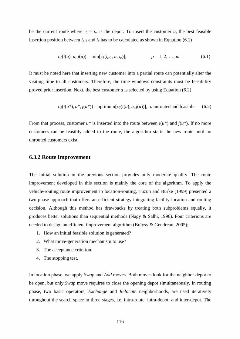
116
be the current route where i0 = im is the depot. To insert the customer u, the best feasible
insertion position between ip-1 and ip has to be calculated as shown in Equation (6.1)
c1(i(u), u, j(u)) = min[c1(ip-1, u, ip)], p = 1, 2, …, m (6.1)
It must be noted here that inserting new customer into a partial route can potentially alter the
visiting time to all customers. Therefore, the time windows constraints must be feasibility
proved prior insertion. Next, the best customer u is selected by using Equation (6.2)
c2(i(u*), u*, j(u*)) = optimum[c2(i(u), u, j(u))], u unrouted and feasible (6.2)
From that process, customer u* is inserted into the route between i(u*) and j(u*). If no more
customers can be feasibly added to the route, the algorithm starts the new route until no
unrouted customers exist.
6.3.2 Route Improvement
The initial solution in the previous section provides only moderate quality. The route
improvement developed in this section is mainly the core of the algorithm. To apply the
vehicle-routing route improvement in location-routing, Tuzun and Burke (1999) presented a
two-phase approach that offers an efficient strategy integrating facility location and routing
decision. Although this method has drawbacks by treating both subproblems equally, it
produces better solutions than sequential methods (Nagy & Salhi, 1996). Four criterions are
needed to design an efficient improvement algorithm (Bräysy & Gendreau, 2005);
1. How an initial feasible solution is generated?
2. What move-generation mechanism to use?
3. The acceptance criterion.
4. The stopping test.
In location phase, we apply Swap and Add moves. Both moves look for the neighbor depot to
be open, but only Swap move requires to close the opening depot simultaneously. In routing
phase, two basic operators, Exchange and Relocate neighborhoods, are used iteratively
throughout the search space in three stages, i.e. intra-route, intra-depot, and inter-depot. The
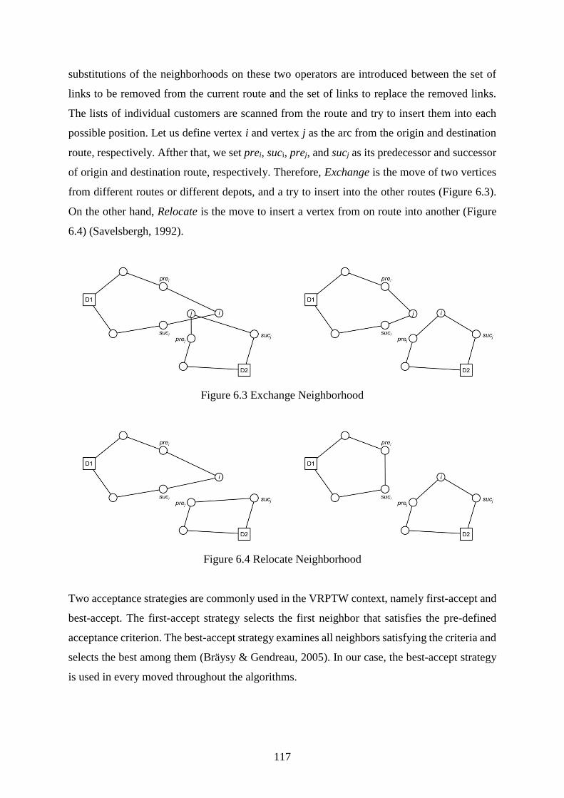
117
substitutions of the neighborhoods on these two operators are introduced between the set of
links to be removed from the current route and the set of links to replace the removed links.
The lists of individual customers are scanned from the route and try to insert them into each
possible position. Let us define vertex i and vertex j as the arc from the origin and destination
route, respectively. Afther that, we set prei, suci, prej, and sucj as its predecessor and successor
of origin and destination route, respectively. Therefore, Exchange is the move of two vertices
from different routes or different depots, and a try to insert into the other routes (Figure 6.3).
On the other hand, Relocate is the move to insert a vertex from on route into another (Figure
6.4) (Savelsbergh, 1992).
Figure 6.3 Exchange Neighborhood
Figure 6.4 Relocate Neighborhood
Two acceptance strategies are commonly used in the VRPTW context, namely first-accept and
best-accept. The first-accept strategy selects the first neighbor that satisfies the pre-defined
acceptance criterion. The best-accept strategy examines all neighbors satisfying the criteria and
selects the best among them (Bräysy & Gendreau, 2005). In our case, the best-accept strategy
is used in every moved throughout the algorithms.
118
When the best move is explored, the parameters are collected in the tabu list for some iteration,
called tabu tenure. We assigned the tenure equal to 5, meaning that they are forbidden during
the next five moves. To escape from a local minima, we set the aspiration criteria allowing a
move (even if it is tabu) if it produces a better solution (Gendreau & Potvin, 2010).
One of the drawbacks of local search approaches is that they try to search only the local space
as the name implies (Gendreau & Potvin, 2010). Even a good solution is found; one cannot
ensure whether the other search space can produce a better solution. To encounter this issue,
we introduce one of the diversification techniques, called “restart diversification” forcing the
search to escape from the best-known solution and examining the area that has not yet been
explored. It can be achieved by restarting the searches in location phase and look for the
unopened depots and continue the routing phase simultaneously.
6.3.3 Model Validation
The comparison between branch-and-price exact solution from Chapter 4 and tabu search
heuristics solution presents in Table 6.4. The optimal solutions of Tabu search are sub-optimal
as expected. The total cost of Tabu search on average is 2.8% higher than the branch-and-price.
However, it saves up to 98.8% of the computational time. Therefore, it can be said that the
Tabu search algorithm proposed in this research is a promising tool to solve LRPTW instances,
especially with the large size problem.
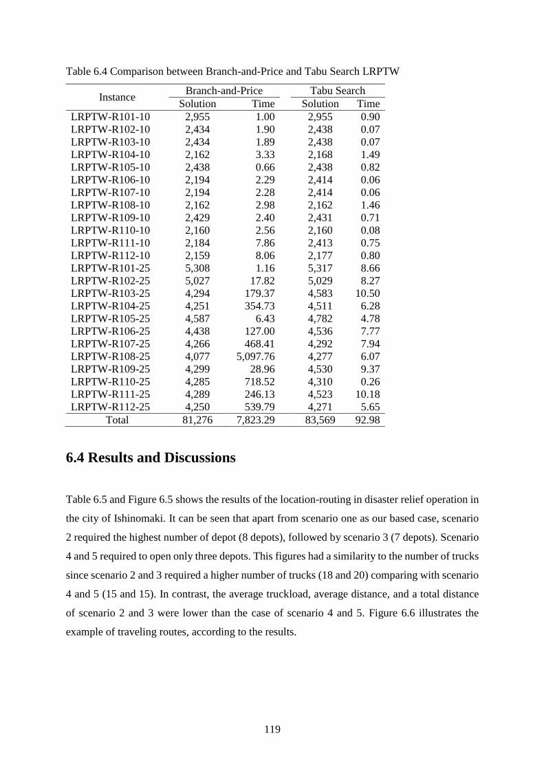
119
Table 6.4 Comparison between Branch-and-Price and Tabu Search LRPTW
Instance Branch-and-Price Tabu Search
Solution Time Solution Time
LRPTW-R101-10 2,955 1.00 2,955 0.90
LRPTW-R102-10 2,434 1.90 2,438 0.07
LRPTW-R103-10 2,434 1.89 2,438 0.07
LRPTW-R104-10 2,162 3.33 2,168 1.49
LRPTW-R105-10 2,438 0.66 2,438 0.82
LRPTW-R106-10 2,194 2.29 2,414 0.06
LRPTW-R107-10 2,194 2.28 2,414 0.06
LRPTW-R108-10 2,162 2.98 2,162 1.46
LRPTW-R109-10 2,429 2.40 2,431 0.71
LRPTW-R110-10 2,160 2.56 2,160 0.08
LRPTW-R111-10 2,184 7.86 2,413 0.75
LRPTW-R112-10 2,159 8.06 2,177 0.80
LRPTW-R101-25 5,308 1.16 5,317 8.66
LRPTW-R102-25 5,027 17.82 5,029 8.27
LRPTW-R103-25 4,294 179.37 4,583 10.50
LRPTW-R104-25 4,251 354.73 4,511 6.28
LRPTW-R105-25 4,587 6.43 4,782 4.78
LRPTW-R106-25 4,438 127.00 4,536 7.77
LRPTW-R107-25 4,266 468.41 4,292 7.94
LRPTW-R108-25 4,077 5,097.76 4,277 6.07
LRPTW-R109-25 4,299 28.96 4,530 9.37
LRPTW-R110-25 4,285 718.52 4,310 0.26
LRPTW-R111-25 4,289 246.13 4,523 10.18
LRPTW-R112-25 4,250 539.79 4,271 5.65
Total 81,276 7,823.29 83,569 92.98
6.4 Results and Discussions
Table 6.5 and Figure 6.5 shows the results of the location-routing in disaster relief operation in
the city of Ishinomaki. It can be seen that apart from scenario one as our based case, scenario
2 required the highest number of depot (8 depots), followed by scenario 3 (7 depots). Scenario
4 and 5 required to open only three depots. This figures had a similarity to the number of trucks
since scenario 2 and 3 required a higher number of trucks (18 and 20) comparing with scenario
4 and 5 (15 and 15). In contrast, the average truckload, average distance, and a total distance
of scenario 2 and 3 were lower than the case of scenario 4 and 5. Figure 6.6 illustrates the
example of traveling routes, according to the results.
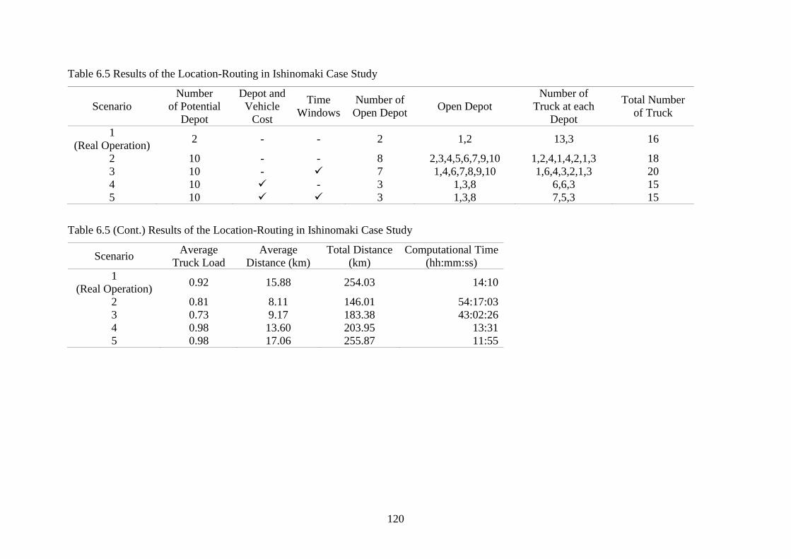
120
Table 6.5 Results of the Location-Routing in Ishinomaki Case Study
Scenario
Number
of Potential
Depot
Depot and
Vehicle
Cost
Time
Windows
Number of
Open Depot Open Depot
Number of
Truck at each
Depot
Total Number
of Truck
1
(Real Operation) 2 - - 2 1,2 13,3 16
2 10 - - 8 2,3,4,5,6,7,9,10 1,2,4,1,4,2,1,3 18
3 10 - 7 1,4,6,7,8,9,10 1,6,4,3,2,1,3 20
4 10 - 3 1,3,8 6,6,3 15
5 10 3 1,3,8 7,5,3 15
Table 6.5 (Cont.) Results of the Location-Routing in Ishinomaki Case Study
Scenario Average
Truck Load
Average
Distance (km)
Total Distance
(km)
Computational Time
(hh:mm:ss)
1
(Real Operation) 0.92 15.88 254.03 14:10
2 0.81 8.11 146.01 54:17:03
3 0.73 9.17 183.38 43:02:26
4 0.98 13.60 203.95 13:31
5 0.98 17.06 255.87 11:55
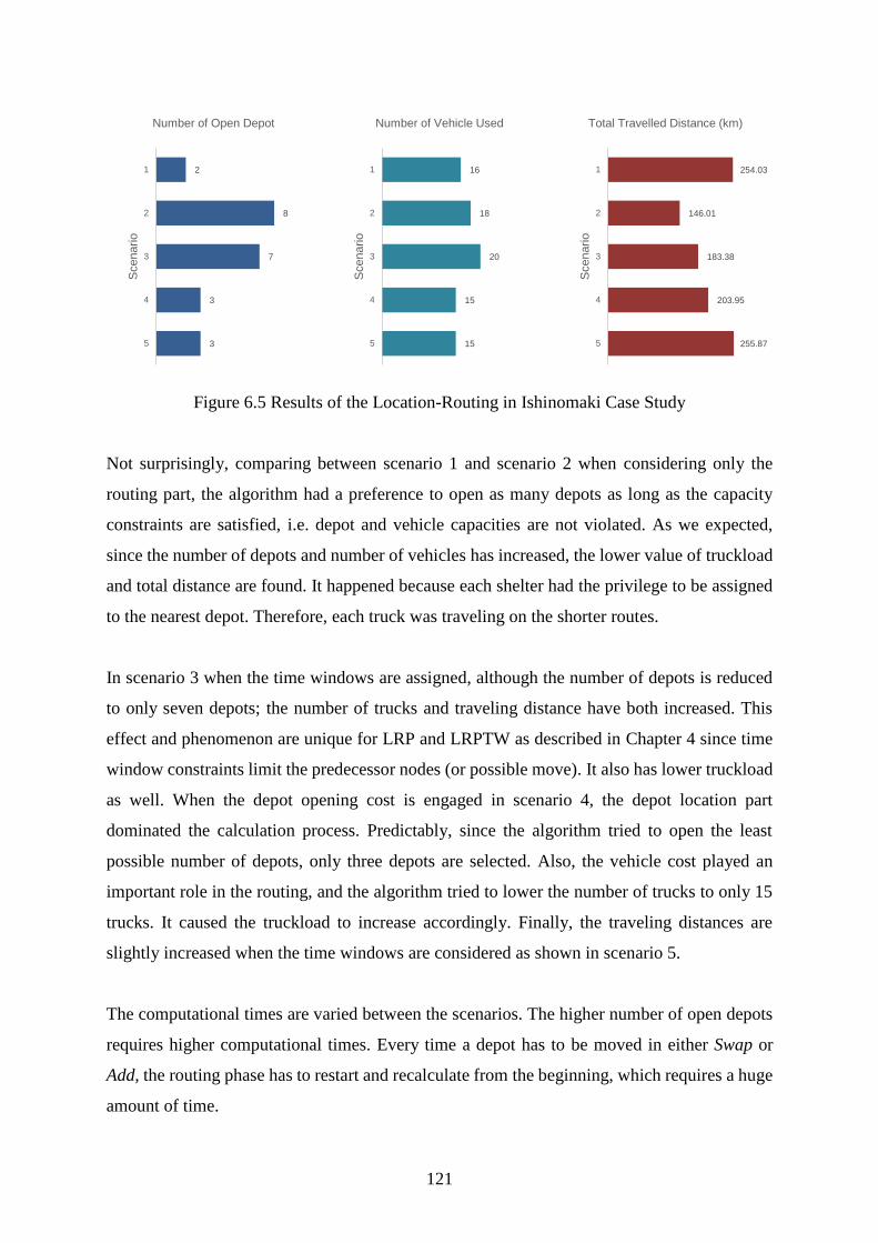
121
Figure 6.5 Results of the Location-Routing in Ishinomaki Case Study
Not surprisingly, comparing between scenario 1 and scenario 2 when considering only the
routing part, the algorithm had a preference to open as many depots as long as the capacity
constraints are satisfied, i.e. depot and vehicle capacities are not violated. As we expected,
since the number of depots and number of vehicles has increased, the lower value of truckload
and total distance are found. It happened because each shelter had the privilege to be assigned
to the nearest depot. Therefore, each truck was traveling on the shorter routes.
In scenario 3 when the time windows are assigned, although the number of depots is reduced
to only seven depots; the number of trucks and traveling distance have both increased. This
effect and phenomenon are unique for LRP and LRPTW as described in Chapter 4 since time
window constraints limit the predecessor nodes (or possible move). It also has lower truckload
as well. When the depot opening cost is engaged in scenario 4, the depot location part
dominated the calculation process. Predictably, since the algorithm tried to open the least
possible number of depots, only three depots are selected. Also, the vehicle cost played an
important role in the routing, and the algorithm tried to lower the number of trucks to only 15
trucks. It caused the truckload to increase accordingly. Finally, the traveling distances are
slightly increased when the time windows are considered as shown in scenario 5.
The computational times are varied between the scenarios. The higher number of open depots
requires higher computational times. Every time a depot has to be moved in either Swap or
Add, the routing phase has to restart and recalculate from the beginning, which requires a huge
amount of time.
2
8
7
3
3
1
2
3
4
5
Scenario
Number of Open Depot
16
18
20
15
15
1
2
3
4
5
Scenario
Number of Vehicle Used
254.03
146.01
183.38
203.95
255.87
1
2
3
4
5
Scenario
Total Travelled Distance (km)
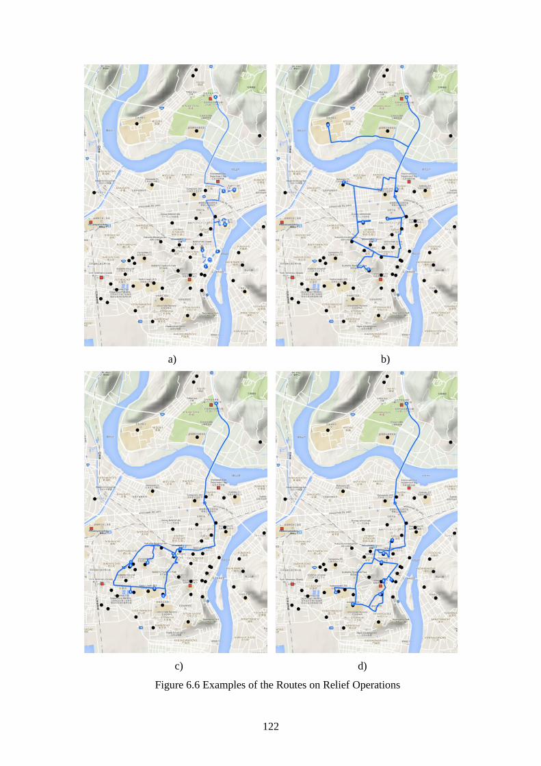
122
a) b)
c) d)
Figure 6.6 Examples of the Routes on Relief Operations
123
References
Badeau, P. et al., 1997. A parallel tabu search heuristic for the vehicle routing problem with
time windows. Transportation Research Part C: Emerging Technologies, 5(2), pp. 109-
122.
Brandão, J., 1999. Metaheuristic for the vehicle routing problem with time windows. In:
Meta-Heuristics. Springer US, pp. 19-36.
Bräysy, O. & Gendreau, M., 2005. Vehicle routing problem with time windows, Part I: Route
construction and local search algorithms. Transportation Science, 39(1), pp. 104-118.
Burks Jr., R. E., 2006. An adaptive tabu search heuristic for the location routing pickup and
delivery problem with time windows with a theater distribution application, Ohio: Air
Force Institute of Technology.
Carlton, W. B., 1995. A tabu search approach to the general vehicle routing problem, Texas:
Doctoral dissertation, University of Texas at Austin.
Chiang, W. C. & Russell, R. A., 1997. A reactive tabu search metaheuristic for the vehicle
routing problem with time windows. INFORMS Journal on Computing, 9(4), pp. 417-
430.
Cordeau, J. F., Laporte, G. & Mercier, A., 2001. A unified tabu search heuristic for vehicle
routing problems with time windows. Journal of the Operational Research Society, 52(8),
pp. 928-936.
De Backer, B. & Furnon, V., 1997. Meta-heuristics in constraint programming experiments
with tabu search on the vehicle routing problem. Sophia Antipolis, France, Second
International Conference on Metaheuristics (MIC 97).
Desaulniers, G., Lessard, F. & Hadjar, A., 2008. Tabu search, partial elementarity, and
generalized k-path inequalities for the vehicle routing problem with time windows.
Transportation Science, 42(3), pp. 387-404.
Garcia, B. L., Potvin, J. Y. & Rousseau, J. M., 1994. A parallel implementation of the tabu
search heuristic for vehicle routing problems with time window constraints. Computers &
Operations Research, 21(9), pp. 1025-1033.
Gendreau, M., 2003. An Introduction to Tabu Search. Springer US.
Gendreau, M. & Potvin, J. Y., 2010. Handbook of Metaheuristics. Vol. 2 ed. New York:
Springer.
Glover, F., 1977. Heuristics for integer programming using surrogate constraints. Decision
Sciences, 8(1), pp. 156-166.
124
Glover, F., 1989. Tabu search-part I. ORSA Journal on Computing, 1(3), pp. 190-206.
Glover, F., 1990. Tabu search—part II. ORSA Journal on Computing, 2(1), pp. 4-32.
Glover, F. & Laguna, M., 1997. Tabu search. Massachusetts: Kluwer Academic Publishers.
Glover, F. & Laguna, M., 1999. Tabu search. Springer US.
Gündüz, H. I., 2011. The Single-Stage Location-Routing Problem with Time Windows. In: J.
W. Böse, et al. eds. Computational Logistics. Hamburg: Springer Berlin Heidelberg, pp.
44-58.
Hertz, A., Taillard, E. & De Werra, D., 1997. Tabu search. In: E. Aarts & J. K. Lenstra, eds.
Local Search in Combinatorial Optimization. Chichester: John Wiley and Sons, pp. 121-
136.
Lau, H. C., Lim, Y. F. & Liu, Q., 2001. Diversification of neighborhood via constraint-based
local search and its application to VRPTW. s.l., Proc. CP-AI-OR 2001 Workshop.
Lau, H. C., Sim, M. & Teo, K. M., 2003. Vehicle routing problem with time windows and a
limited number of vehicles. European Journal of Operational Research, 148(3), pp. 559-
569.
Mertens, S., 1999. TSP Algorithms in Action Animated Examples of Heuristic Algorithms.
[Online] Available at: http://www-e.uni-magdeburg.de/mertens/TSP/TSP.html [Accessed
10 5 2015].
Nagy, G. & Salhi, S., 1996. Nested heuristic methods for the location-routeing problem.
Journal of the Operational Research Society, Volume 47, pp. 1166-1174.
Nakanishi, H., Matsuo, K. & Black, J., 2013. Transportation planning methodologies for
post-disaster recovery in regional communities: the East Japan Earthquake and tsunami
2011. Journal of Transport Geography, Volume 31, pp. 181-191.
Osman, I. H., 1993. Metastrategy simulated annealing and tabu search algorithms for the
vehicle routing problem. Annals of operations research, 41(4), pp. 421-451.
Ponboon, S., Taniguchi, E. & Qureshi, A. G., 2013. Integrated Approach for Location-
Routing Problem using Branch-and-Price Method. Hiroshima, JSCE 47th Conference on
Infrastructure Planning and Management.
Potvin, J. Y. & Bengio, S., 1996. The vehicle routing problem with time windows part II:
genetic search. INFORMS Journal on Computing, 8(2), pp. 165-172.
Rochat, Y. & Taillard, E. D., 1995. Probabilistic diversification and intensification in local
search for vehicle routing. Journal of Heuristics, 1(1), pp. 147-167.
Savelsbergh, M. W., 1992. The vehicle routing problem with time windows: Minimizing
route duration. ORSA Journal on Computing, 4(2), pp. 146-154.
125
Schittekat, P. & Sorensen, K., 2009. Or practice - supporting 3PL decisions in the automotive
industry by generating diverse solutions to a large-scale location-routing problem.
Operations Research, Volume 57(5), pp. 1058-1067.
Schulze, J. & Fahle, T., 1999. A parallel algorithm for the vehicle routing problem with time
window constraints. Annals of Operations Research, Volume 86, pp. 585-607.
Semet, F. & Taillard, E., 1993. Solving real-life vehicle routing problems efficiently using
tabu search. Annals of Operations Research, Volume 41, p. 469–488.
Taillard, E. et al., 1997. A tabu search heuristic for the vehicle routing problem with soft time
windows. Transportation Science, 31(2), pp. 170-186.
Taniguchi, E. & Thompson, R. G., 2013. Humanitarian Logistics in the Great Tohoku
Disasters 2011. In: V. Zeimpekis, S. Ichoua & I. Minis, eds. Humanitarian and Relief
Logistics. New York: Springer, pp. 207-218.
Tan, K. C., Lee, L. H., Zhu, Q. L. & Ou, K., 2001. Heuristic methods for vehicle routing
problem with time windows. Artificial Intelligence in Engineering, 15(3), pp. 281-295.
Tuzun, D. & Burke, L. I., 1999. A two-phase tabu search approach to the location routing
problem. European Journal of Operational Research, 116(1), pp. 87-99.

126
127
Chapter 7
Conclusion and Recommendation
7.1 Conclusions
7.1.1 Branch-and-Price Algorithm for LRPTW
7.1.2 LRPTW in Osaka Distribution Network
7.1.3 LRPTW in Ishinomaki Humanitarian Logistics
7.2 Future Works

128
129
7.1 Conclusions
7.1.1 Branch-and-Price Algorithm for LRPTW
This paper presents the framework to integrate the facility location and the vehicle
routing problems with time windows. The location-routing problem (LRP) is attracting
many researchers and practitioners since it allows manipulating the mathematical
problem in both strategic and operational levels. The combination of location-routing
and time windows (LRPTW) has never been attempted before using an exact algorithm.
This study proposes the method of decomposing the complex integer programming
formulation of the LRPTW into master and subproblems and contributes the new
column generation based algorithm to solve it.
New test instances for the LRPTW are generated from the VRPTW Solomon
benchmark instances to evaluate the performance, with the first 10- and 25-customer.
The original depot is replaced by the new three potential depot sites together with other
parameters used in the LRPTW formulations. It proves that the new exact algorithm
proposed in this research can solve the LRPTW instances to optimality within an
acceptable time. It shows in the previous section that the exact solutions of the LRPTW
can reduce the required number of trucks as well as the distance traveled as compared
to the exact VRPTW solutions. Therefore, further emphasizes the importance of the
LRPTW and the advantage of an exact solution approach for this variation. Also, the
characteristics of the time window constraints affecting the location and routing
processes in the LRPTW are also intensively explored and reported.
7.1.2 LRPTW in Osaka Distribution Network
This topic presents the evaluation of cost structure of different environmental factors of
LRPTW, which is rarely examined by the exact algorithm. The branch-and-price
algorithm is implemented to ensure that the quality of the solution is reliable. The
distribution network is extracted from the real operation of logistics firm in Osaka
while the travel time is collected by the GPS and the traffic census data of the Osaka
city. The main decision factors for LRPTW are the location of the depot, depot size,
130
and vehicle size. It is found that the large size depot together with the large size vehicle
scenario is among the best scheme in our case study. The depot located in Minato-ku is
the best location for the large size depot scenario by the fact that it is located in the low-
price area. Furthermore, the large size vehicle of the 3-ton vehicle is proved to be the
best choice. Regardless of the highest vehicle fixed cost, the number of the vehicle can
be reduced to only seven vehicles, but remain the high truckload, making the lowest
delivered cost option.
7.1.3 LRPTW in Ishinomaki Humanitarian Logistics
This study presented two computational algorithms to solve the location-routing
problem with time windows for disaster relief operations. The algorithm bases on the
tabu search heuristics. The location and routing phases are separately considered using
simple but effective operators. The process ends when no other beneficial moves are
detected. We obtain the results from the branch-and-price algorithm as a benchmark for
tabu search algorithm. After that, we use the latter for solving the large size real-world
problems.
The city of Ishinomaki is a case study. It is attacked by the tsunami triggered from the
great Japanese earthquake on March 11, 2011. 3,417 people were killed. 53,742 houses
were destroyed and left 30,930 people displace. The developed Tabu search is used to
determine the refugee center or depots to store food and important commodities for the
people. Apart from the two depot locations used in the real operation, we propose eight
more potential locations throughout the city and determine the optimal locations in four
different scenarios. The results are expected to provide the broader perspective on how
mathematical models can support the humanitarian logistics in disaster relief operation.
7.2 Future Works
The exact algorithms are usually computationally expensive comparing with
approximate methods. Same is the case with our proposed algorithm, and it becomes
much harder to solve the larger problems, especially with wider time windows. The
combination of exact and metaheuristic approaches as a hybrid algorithm is, therefore,
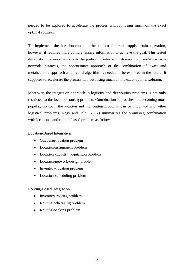
131
needed to be explored to accelerate the process without losing much on the exact
optimal solution.
To implement the location-routing scheme into the real supply chain operation,
however, it requires more comprehensive information to achieve the goal. This tested
distribution network limits only the portion of selected customers. To handle the large
network instances, the approximate approach or the combination of exact and
metaheuristic approach as a hybrid algorithm is needed to be explored in the future. It
supposes to accelerate the process without losing much on the exact optimal solution.
Moreover, the integration approach in logistics and distribution problems is not only
restricted to the location-routing problem. Combination approaches are becoming more
popular, and both the location and the routing problems can be integrated with other
logistical problems. Nagy and Salhi (2007) summarizes the promising combination
with locational and routing based problem as follows.
Location-Based Integration
Queueing-location problem
Location-assignment problem
Location-capacity-acquisition problem
Location-network-design problem
Inventory-location problem
Location-scheduling problem
Routing-Based Integration
Inventory-routing problem
Routing-scheduling problem
Routing-packing problem

132
133
Appendix A
Optimal Solutions of Modified LRP

134

135
Perl83-12x2 TW
D1 7 3 2 1 6 8 9
4 5 11 12 10
Optimal solution = 204.00
1
2
3
4
5
6
7
8
9
10
11
12
D1
D2
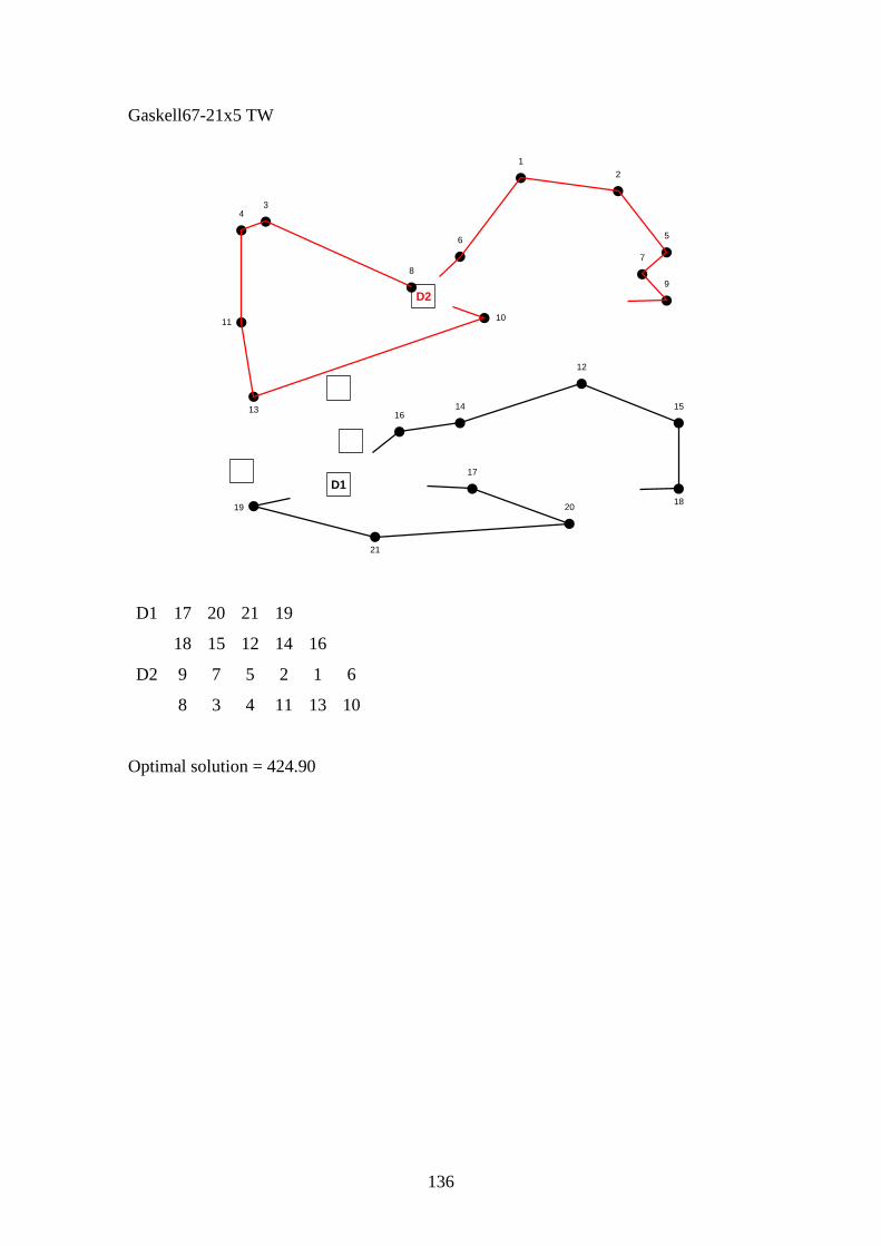
136
Gaskell67-21x5 TW
D1 17 20 21 19
18 15 12 14 16
D2 9 7 5 2 1 6
8 3 4 11 13 10
Optimal solution = 424.90
D1
D2
D3
D4
D5
1
2
34
56
7
8
9
1011
12
13 14 1516
17
1819 20
21
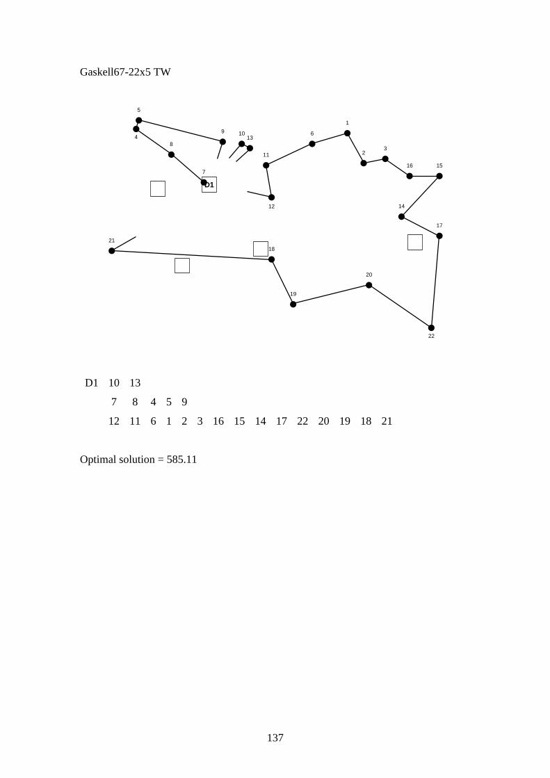
137
Gaskell67-22x5 TW
D1 10 13
7 8 4 5 9
12 11 6 1 2 3 16 15 14 17 22 20 19 18 21
Optimal solution = 585.11
D1
D2
D3
D4
D5
1
23
4
5
6
7
8
9 10
11
12
13
14
1516
17
18
19
20
21
22
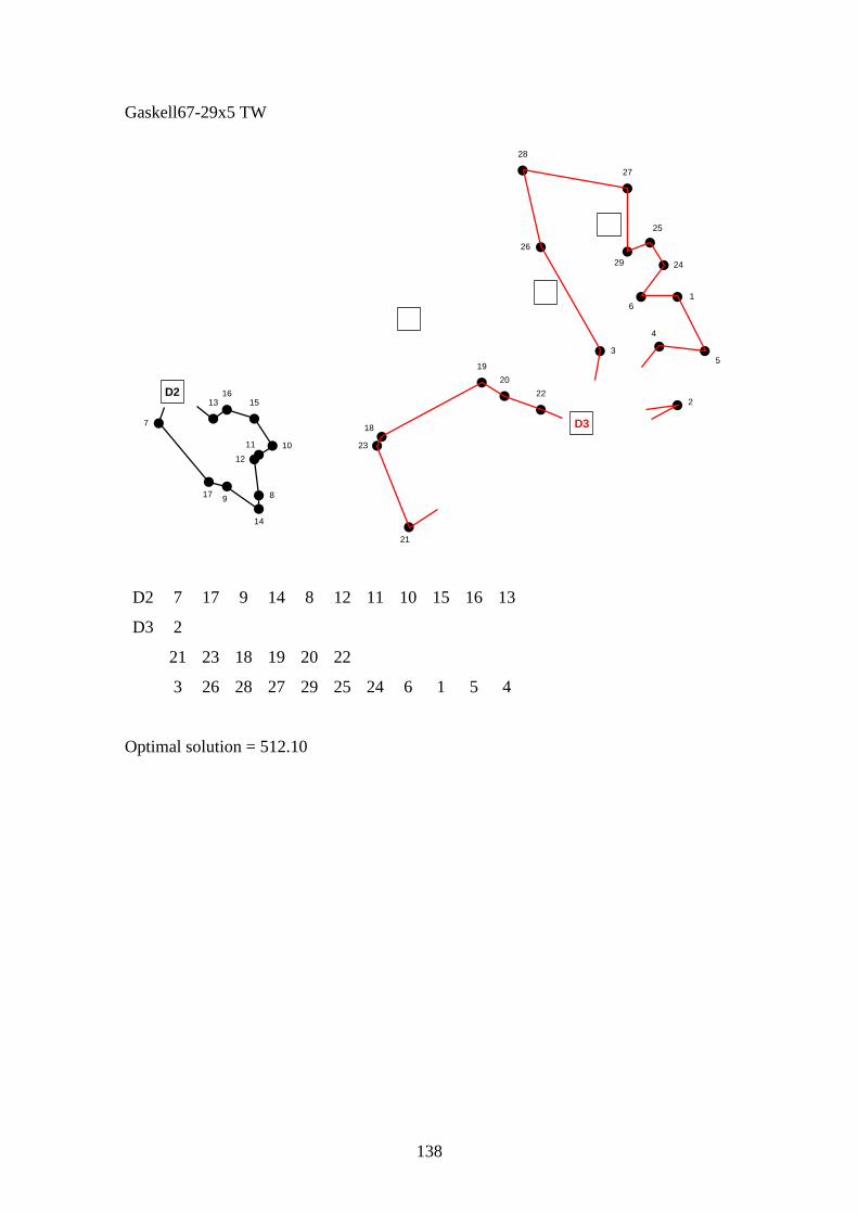
138
Gaskell67-29x5 TW
D2 7 17 9 14 8 12 11 10 15 16 13
D3 2
21 23 18 19 20 22
3 26 28 27 29 25 24 6 1 5 4
Optimal solution = 512.10
D1
D2
D3
D4
D5
1
2
3
4
5
6
7
89
1011
12
13
14
1516
17
18
19
20
21
22
23
24
25
26
27
28
29
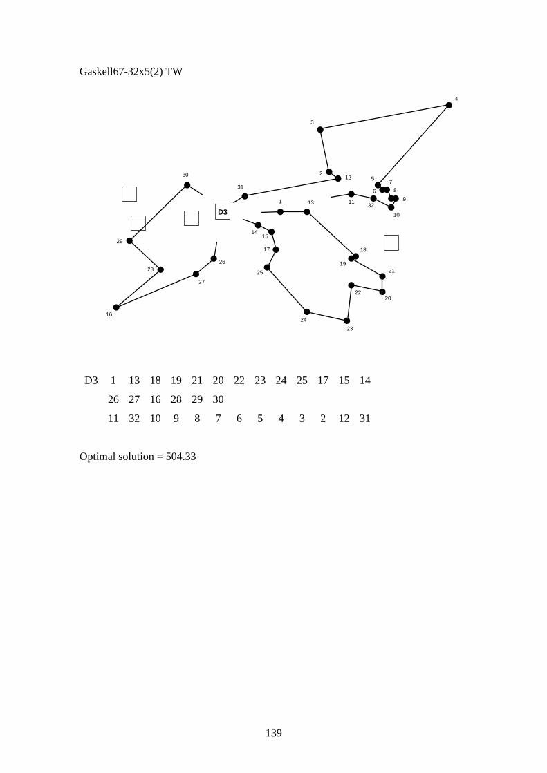
139
Gaskell67-32x5(2) TW
D3 1 13 18 19 21 20 22 23 24 25 17 15 14
26 27 16 28 29 30
11 32 10 9 8 7 6 5 4 3 2 12 31
Optimal solution = 504.33
D1
D2
D3D4
D5
1
2
3
4
5
6
7
8
9
10
11
12
13
1415
16
17 18
19
20
21
22
23
24
25
26
27
28
29
30
31
32

140
Gaskell67-36x5 TW
D5 15 14 8 2 1 7 13 19 20
16 17 18 24 30 36 35 29 23
21 27 26 25 31 32 33 34 28 22
9 3 4 5 6 12 11 10
Optimal solution = 460.37
D1
D2
D3
D4
D5
1
2
3
4
5
6
7
8
9
10
11
12
13
14
15
16
17
18
19
20
21
22
23
24
25
26
27
28
29
30
31
32
33
34
35
36
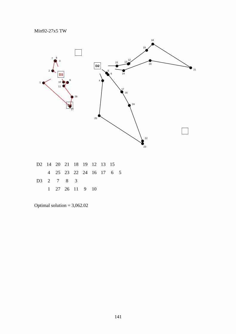
141
Min92-27x5 TW
D2 14 20 21 18 19 12 13 15
4 25 23 22 24 16 17 6 5
D3 2 7 8 3
1 27 26 11 9 10
Optimal solution = 3,062.02
D1
D2
D3
D4
D5
1
2
3
4
5
6
7 8
910
11
1213
14
15
16
17
18
19
20
21
22
23
24
25
26
27

142
143
Appendix B
Optimal Solutions
of Modified Solomon’s Benchmarks

144
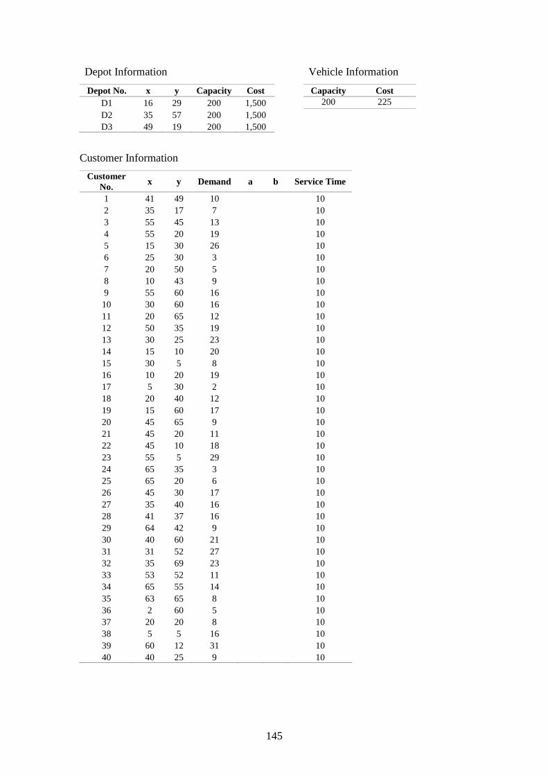
145
Depot Information Vehicle Information
Depot No. x y Capacity Cost Capacity Cost
D1 16 29 200 1,500 200 225
D2 35 57 200 1,500
D3 49 19 200 1,500
Customer Information
Customer
No. x y Demand a b Service Time
1 41 49 10 10
2 35 17 7 10
3 55 45 13 10
4 55 20 19 10
5 15 30 26 10
6 25 30 3 10
7 20 50 5 10
8 10 43 9 10
9 55 60 16 10
10 30 60 16 10
11 20 65 12 10
12 50 35 19 10
13 30 25 23 10
14 15 10 20 10
15 30 5 8 10
16 10 20 19 10
17 5 30 2 10
18 20 40 12 10
19 15 60 17 10
20 45 65 9 10
21 45 20 11 10
22 45 10 18 10
23 55 5 29 10
24 65 35 3 10
25 65 20 6 10
26 45 30 17 10
27 35 40 16 10
28 41 37 16 10
29 64 42 9 10
30 40 60 21 10
31 31 52 27 10
32 35 69 23 10
33 53 52 11 10
34 65 55 14 10
35 63 65 8 10
36 2 60 5 10
37 20 20 8 10
38 5 5 16 10
39 60 12 31 10
40 40 25 9 10
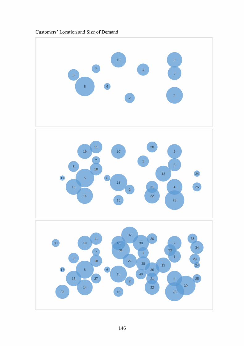
146
Customers’ Location and Size of Demand
1
2
3
4
5 6
7
8
910
1
2
3
4
5 6
7
8
910
11
12
13
14
15
16
17
18
19
20
21
22
23
24
25
1
2
3
4
5 6
7
8
910
11
12
13
14
15
16
17
18
19
20
21
22
23
24
25
26
2728
29
30
31
32
3334
35
36
37
38
39
40
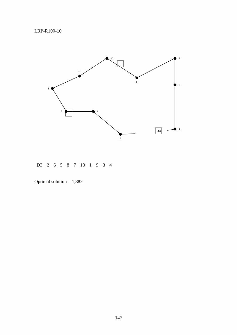
147
LRP-R100-10
D3 2 6 5 8 7 10 1 9 3 4
Optimal solution = 1,882
1
2
3
4
5 6
7
8
910
D1
D2
D3
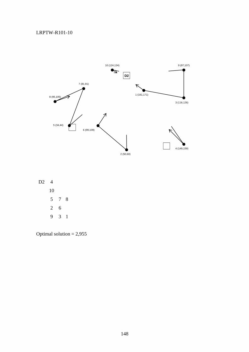
148
LRPTW-R101-10
D2 4
10
5 7 8
2 6
9 3 1
Optimal solution = 2,955
1 (161,171)
2 (50,60)
3 (116,126)
4 (149,159)
5 (34,44)
6 (99,109)
7 (81,91)
8 (95,105)
9 (97,107)10 (124,134)
D1
D2
D3
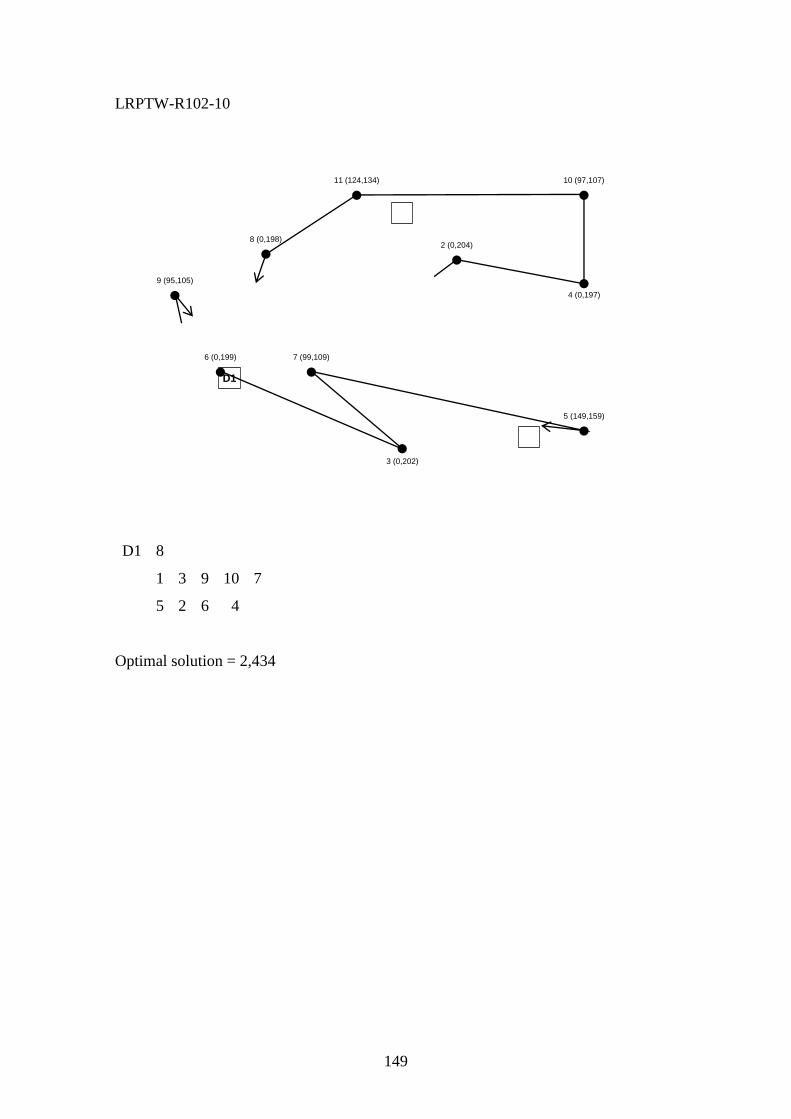
149
LRPTW-R102-10
D1 8
1 3 9 10 7
5 2 6 4
Optimal solution = 2,434
2 (0,204)
3 (0,202)
4 (0,197)
5 (149,159)
6 (0,199) 7 (99,109)
8 (0,198)
9 (95,105)
10 (97,107)11 (124,134)
D1
D2
D3
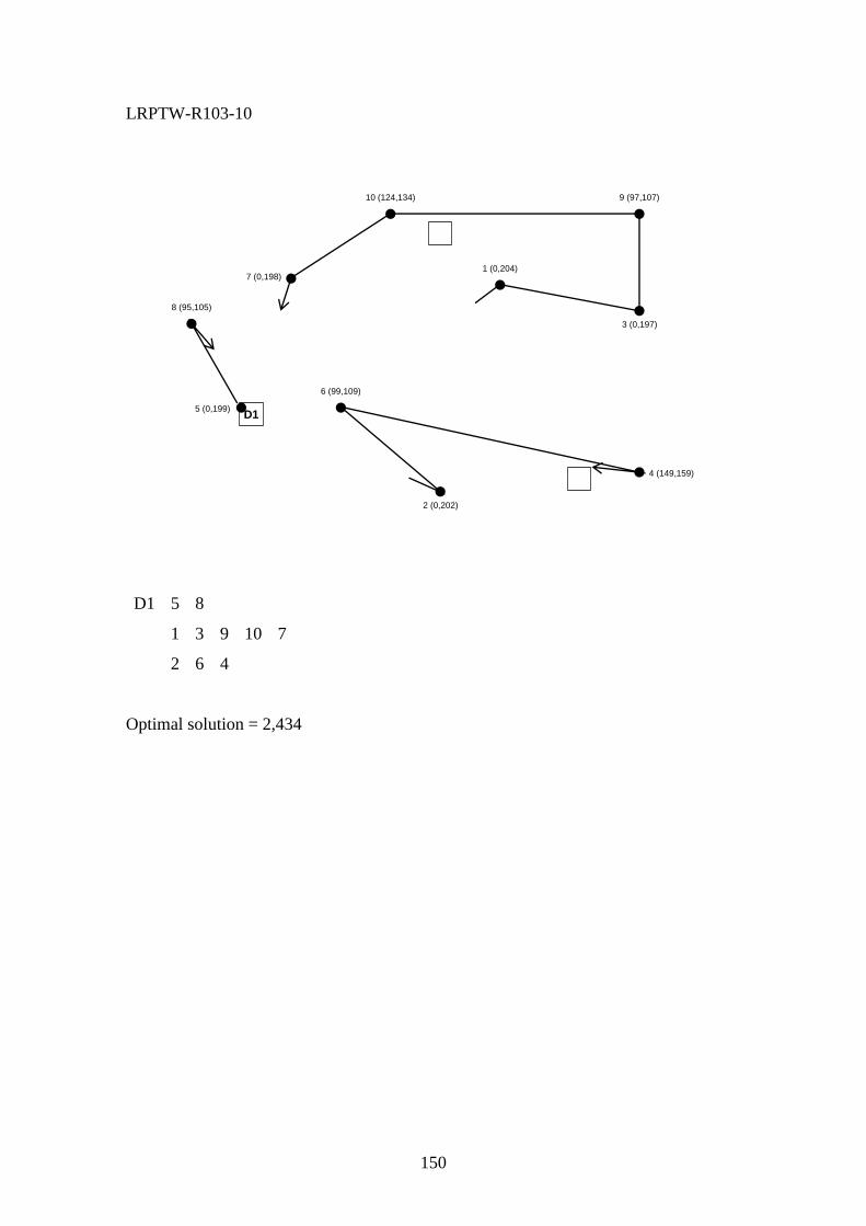
150
LRPTW-R103-10
D1 5 8
1 3 9 10 7
2 6 4
Optimal solution = 2,434
1 (0,204)
2 (0,202)
3 (0,197)
4 (149,159)
5 (0,199)
6 (99,109)
7 (0,198)
8 (95,105)
9 (97,107)10 (124,134)
D1
D2
D3

151
LRPTW-R104-10
D3 3 9 4
1 10 7 8 5 6 2
Optimal solution = 2,162
1 (0,204)
2 (0,202)
3 (0,197)
4 (149,159)
5 (0,199)
6 (0,208)
7 (0,198)
8 (95,105)
9 (97,107)10 (0,194)
D1
D2
D3

152
LRPTW-R105-10
D2 7 8 10
5 2 6 4
9 3 1
Optimal solution = 2,438
1 (151,181)
2 (40,70)
3 (106,136)
4 (139,169)
5 (24,54)
6 (89,119)
7 (71,101)
8 (85,115)
9 (87,117)10 (114,144)
D1
D2
D3
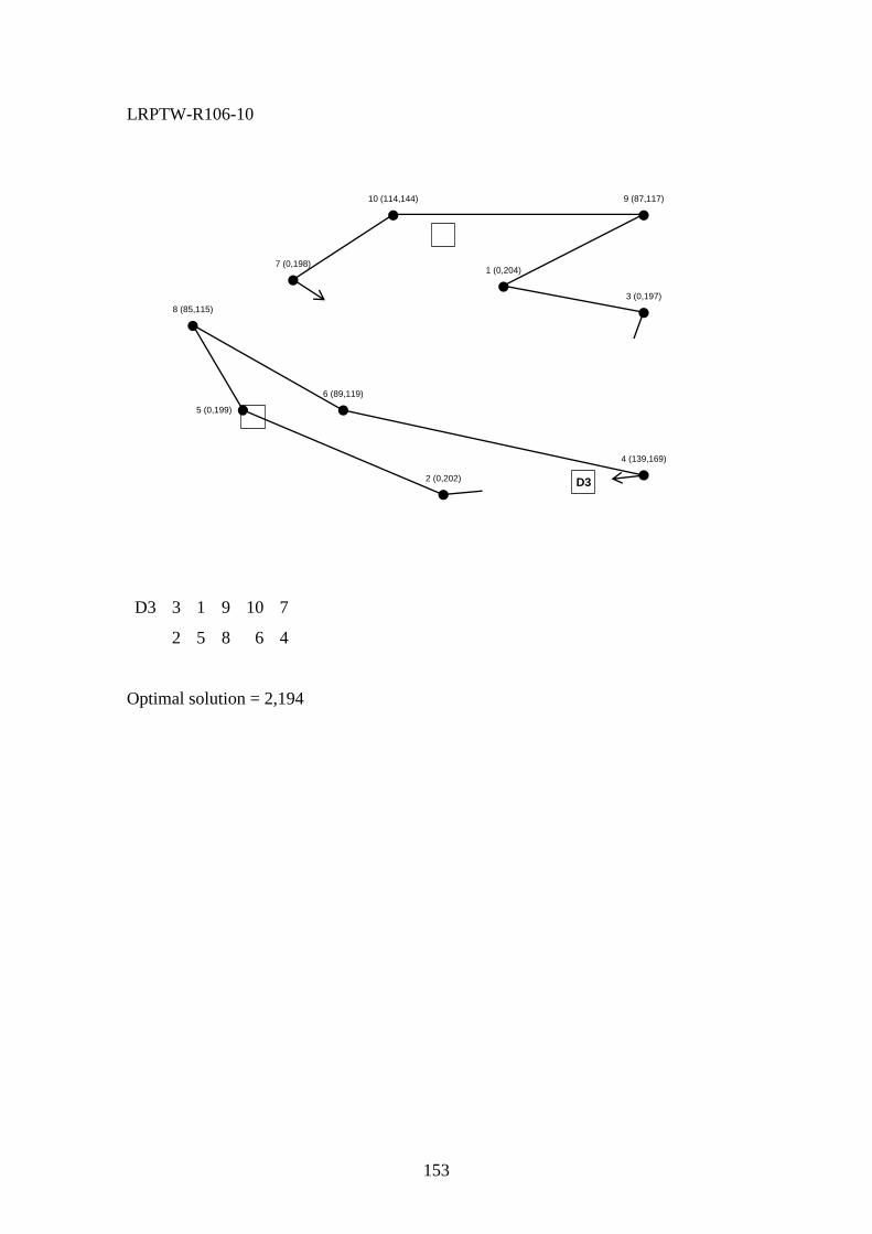
153
LRPTW-R106-10
D3 3 1 9 10 7
2 5 8 6 4
Optimal solution = 2,194
1 (0,204)
2 (0,202)
3 (0,197)
4 (139,169)
5 (0,199)
6 (89,119)
7 (0,198)
8 (85,115)
9 (87,117)10 (114,144)
D1
D2
D3

154
LRPTW-R107-10
D3 3 1 9 10 7
2 5 8 6 4
Optimal solution = 2,194
1 (0,204)
2 (0,202)
3 (0,197)
4 (139,169)
5 (0,199)
6 (89,119)
7 (0,198)
8 (85,115)
9 (87,117)10 (114,144)
D1
D2
D3
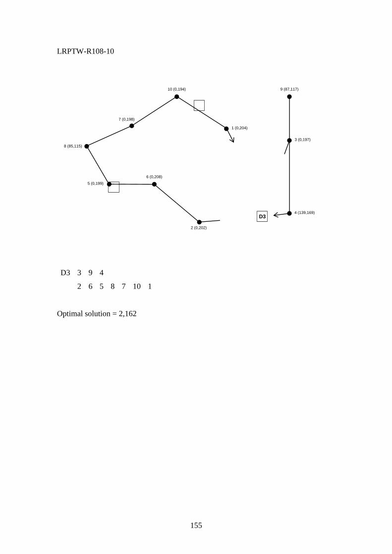
155
LRPTW-R108-10
D3 3 9 4
2 6 5 8 7 10 1
Optimal solution = 2,162
1 (0,204)
2 (0,202)
3 (0,197)
4 (139,169)
5 (0,199)
6 (0,208)
7 (0,198)
8 (85,115)
9 (87,117)10 (0,194)
D1
D2
D3
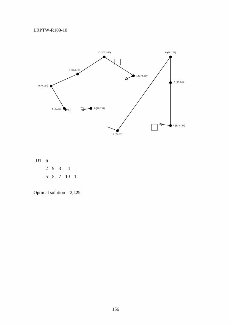
156
LRPTW-R109-10
D1 6
2 9 3 4
5 8 7 10 1
Optimal solution = 2,429
1 (133,198)
2 (22,87)
3 (98,143)
4 (123,184)
5 (20,93) 6 (76,131)
7 (61,110)
8 (75,124)
9 (74,129)10 (107,150)
D1
D2
D3
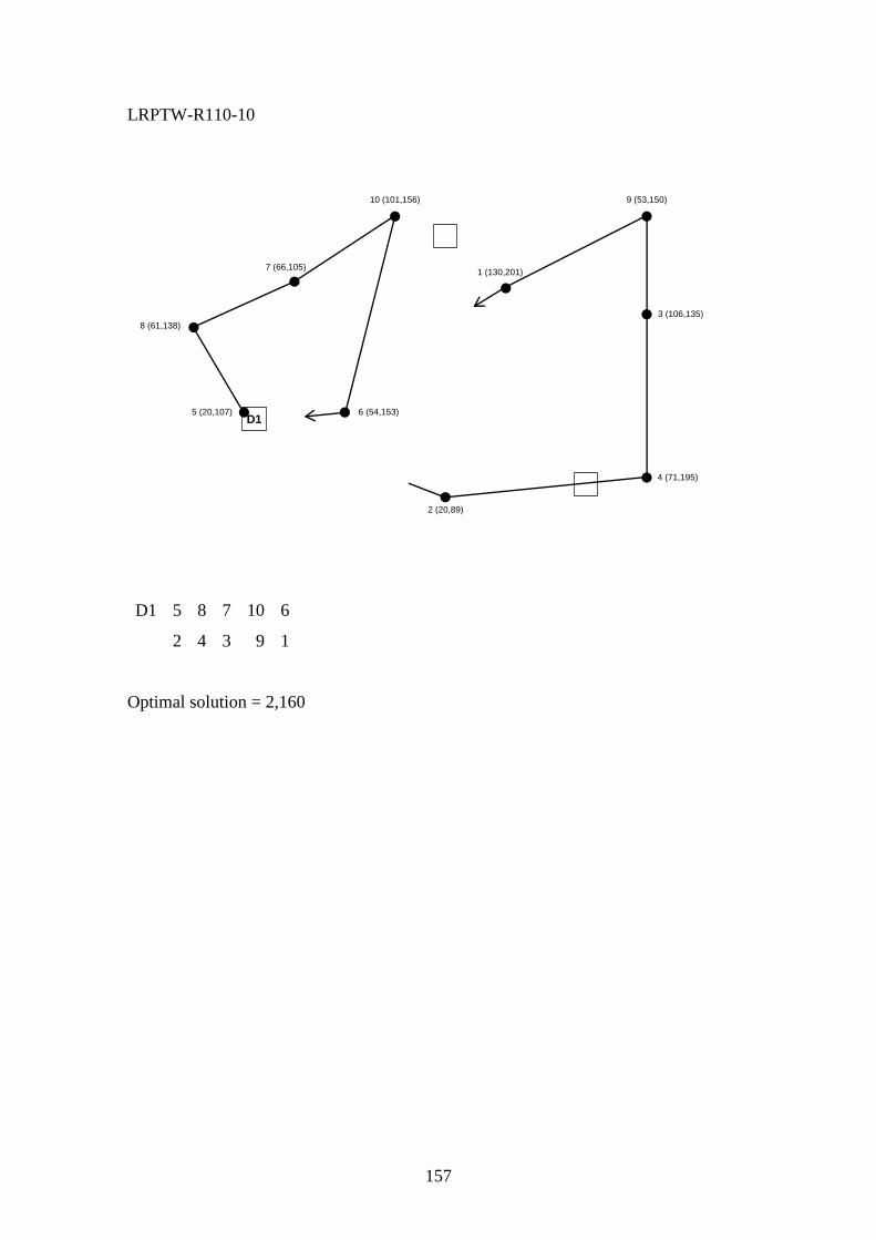
157
LRPTW-R110-10
D1 5 8 7 10 6
2 4 3 9 1
Optimal solution = 2,160
1 (130,201)
2 (20,89)
3 (106,135)
4 (71,195)
5 (20,107) 6 (54,153)
7 (66,105)
8 (61,138)
9 (53,150)10 (101,156)
D1
D2
D3
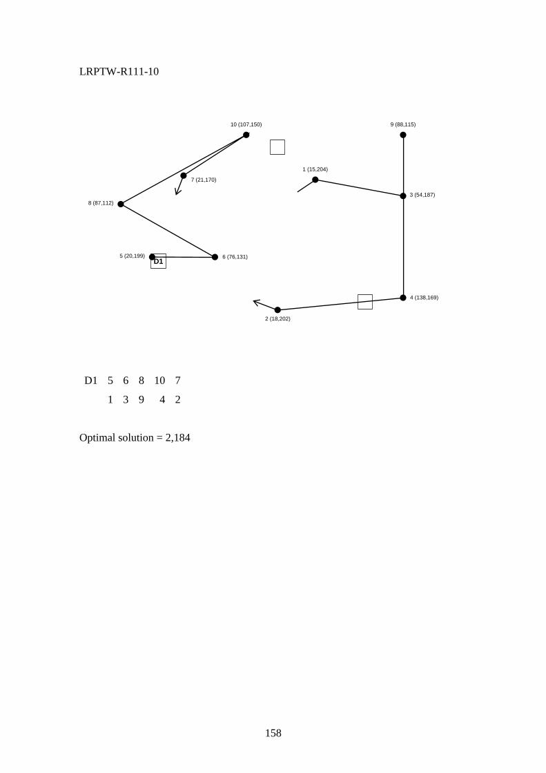
158
LRPTW-R111-10
D1 5 6 8 10 7
1 3 9 4 2
Optimal solution = 2,184
1 (15,204)
2 (18,202)
3 (54,187)
4 (138,169)
5 (20,199) 6 (76,131)
7 (21,170)
8 (87,112)
9 (88,115)10 (107,150)
D1
D2
D3
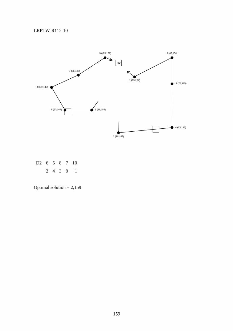
159
LRPTW-R112-10
D2 6 5 8 7 10
2 4 3 9 1
Optimal solution = 2,159
1 (73,204)
2 (18,147)
3 (76,165)
4 (73,195)
5 (20,167) 6 (49,158)
7 (36,135)
8 (50,149)
9 (47,156)10 (85,172)
D1
D2
D3
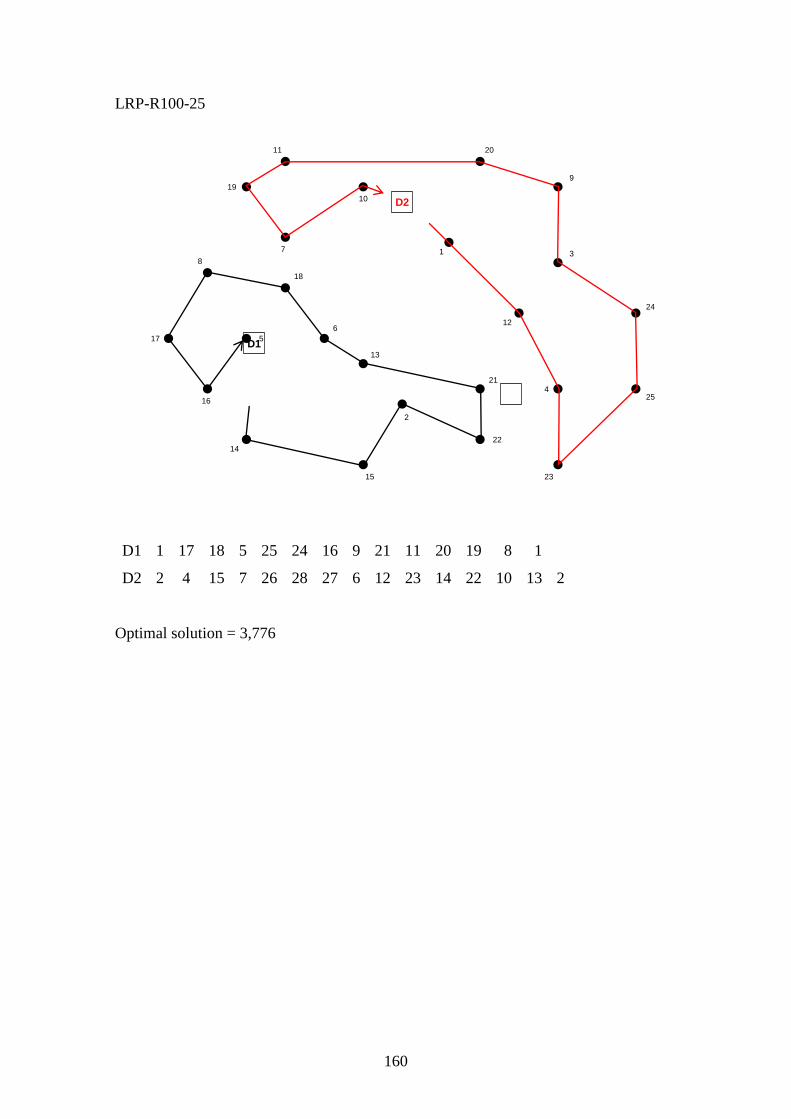
160
LRP-R100-25
D1 1 17 18 5 25 24 16 9 21 11 20 19 8 1
D2 2 4 15 7 26 28 27 6 12 23 14 22 10 13 2
Optimal solution = 3,776
1
2
3
4
5
6
7
8
9
10
11
12
13
14
15
16
17
18
19
20
21
22
23
24
25
D1
D2
D3
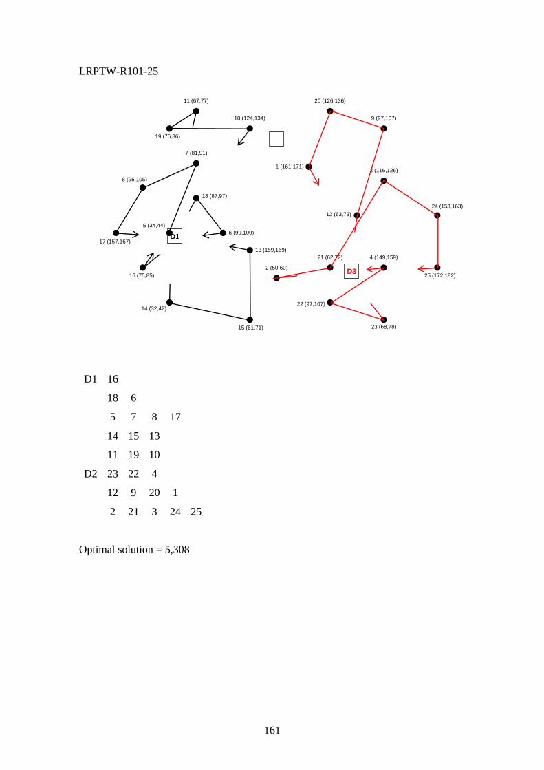
161
LRPTW-R101-25
D1 16
18 6
5 7 8 17
14 15 13
11 19 10
D2 23 22 4
12 9 20 1
2 21 3 24 25
Optimal solution = 5,308
1 (161,171)
2 (50,60)
3 (116,126)
4 (149,159)
5 (34,44)
6 (99,109)
7 (81,91)
8 (95,105)
9 (97,107)10 (124,134)
11 (67,77)
12 (63,73)
13 (159,169)
14 (32,42)
15 (61,71)
16 (75,85)
17 (157,167)
18 (87,97)
19 (76,86)
20 (126,136)
21 (62,72)
22 (97,107)
23 (68,78)
24 (153,163)
25 (172,182)
D1
D2
D3
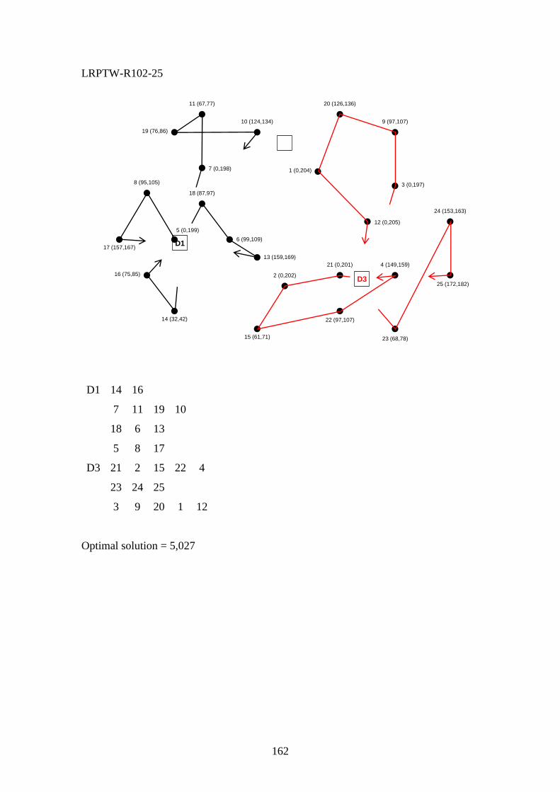
162
LRPTW-R102-25
D1 14 16
7 11 19 10
18 6 13
5 8 17
D3 21 2 15 22 4
23 24 25
3 9 20 1 12
Optimal solution = 5,027
1 (0,204)
2 (0,202)
3 (0,197)
4 (149,159)
5 (0,199)
6 (99,109)
7 (0,198)
8 (95,105)
9 (97,107)10 (124,134)
11 (67,77)
12 (0,205)
13 (159,169)
14 (32,42)
15 (61,71)
16 (75,85)
17 (157,167)
18 (87,97)
19 (76,86)
20 (126,136)
21 (0,201)
22 (97,107)
23 (68,78)
24 (153,163)
25 (172,182)
D1
D2
D3
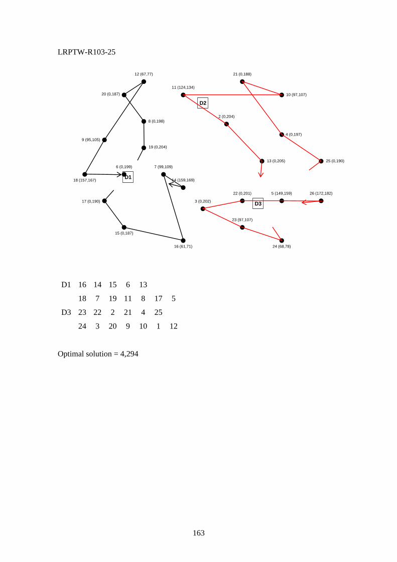
163
LRPTW-R103-25
D1 16 14 15 6 13
18 7 19 11 8 17 5
D3 23 22 2 21 4 25
24 3 20 9 10 1 12
Optimal solution = 4,294
2 (0,204)
3 (0,202)
4 (0,197)
5 (149,159)
6 (0,199) 7 (99,109)
8 (0,198)
9 (95,105)
10 (97,107)
11 (124,134)
12 (67,77)
13 (0,205)
14 (159,169)
15 (0,187)
16 (61,71)
17 (0,190)
18 (157,167)
19 (0,204)
20 (0,187)
21 (0,188)
22 (0,201)
23 (97,107)
24 (68,78)
25 (0,190)
26 (172,182)
D1
D2
D3
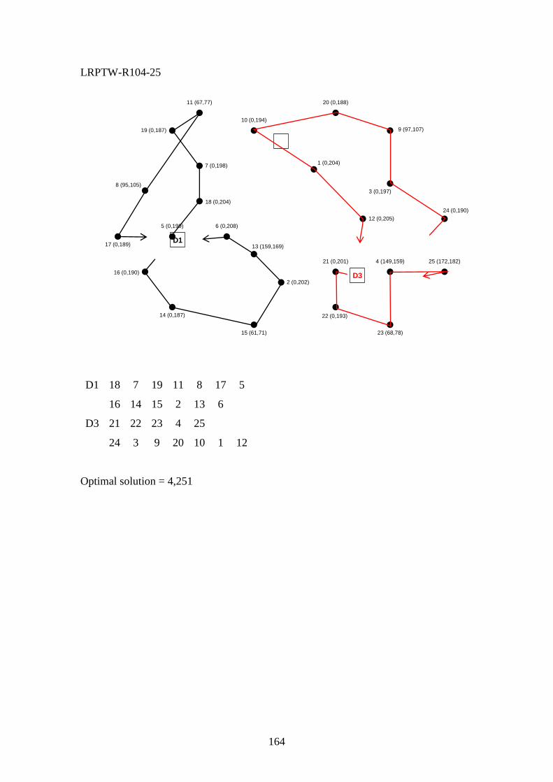
164
LRPTW-R104-25
D1 18 7 19 11 8 17 5
16 14 15 2 13 6
D3 21 22 23 4 25
24 3 9 20 10 1 12
Optimal solution = 4,251
1 (0,204)
2 (0,202)
3 (0,197)
4 (149,159)
5 (0,199) 6 (0,208)
7 (0,198)
8 (95,105)
9 (97,107)
10 (0,194)
11 (67,77)
12 (0,205)
13 (159,169)
14 (0,187)
15 (61,71)
16 (0,190)
17 (0,189)
18 (0,204)
19 (0,187)
20 (0,188)
21 (0,201)
22 (0,193)
23 (68,78)
24 (0,190)
25 (172,182)
D1
D2
D3
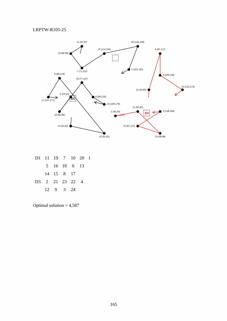
165
LRPTW-R105-25
D1 11 19 7 10 20 1
5 16 18 6 13
14 15 8 17
D3 2 21 23 22 4
12 9 3 24
Optimal solution = 4,587
1 (151,181)
2 (40,70)
3 (106,136)
4 (139,169)
5 (24,54)6 (89,119)
7 (71,101)8 (85,115)
9 (87,117)10 (114,144)
11 (57,87)
12 (53,83)
13 (149,179)
14 (32,62)
15 (51,81)
16 (65,95)
17 (147,177)
18 (77,107)
19 (66,96)
20 (116,146)
21 (52,82)
22 (87,117)
23 (58,88)
24 (143,173)
D1
D2
D3
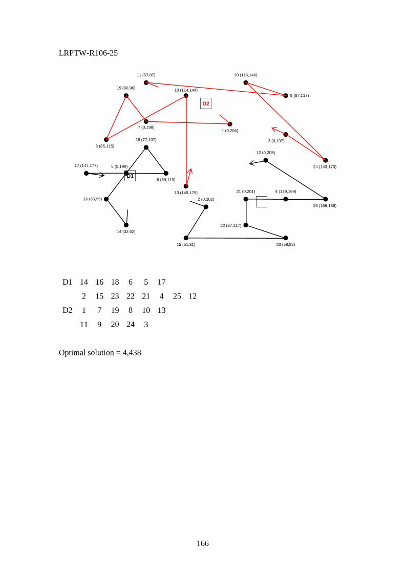
166
LRPTW-R106-25
D1 14 16 18 6 5 17
2 15 23 22 21 4 25 12
D2 1 7 19 8 10 13
11 9 20 24 3
Optimal solution = 4,438
1 (0,204)
2 (0,202)
3 (0,197)
4 (139,169)
5 (0,199)
6 (89,119)
7 (0,198)
8 (85,115)
9 (87,117)
10 (114,144)
11 (57,87)
12 (0,205)
13 (149,179)
14 (32,62)
15 (51,81)
16 (65,95)
17 (147,177)
18 (77,107)
19 (66,96)
20 (116,146)
21 (0,201)
22 (87,117)
23 (58,88)
24 (143,173)
25 (156,186)
D1
D2
D3
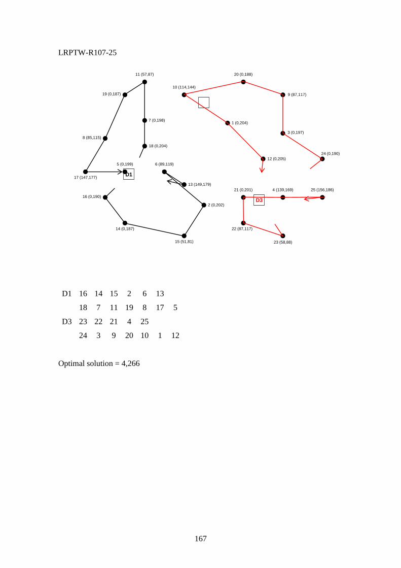
167
LRPTW-R107-25
D1 16 14 15 2 6 13
18 7 11 19 8 17 5
D3 23 22 21 4 25
24 3 9 20 10 1 12
Optimal solution = 4,266
1 (0,204)
2 (0,202)
3 (0,197)
4 (139,169)
5 (0,199) 6 (89,119)
7 (0,198)
8 (85,115)
9 (87,117)
10 (114,144)
11 (57,87)
12 (0,205)
13 (149,179)
14 (0,187)
15 (51,81)
16 (0,190)
17 (147,177)
18 (0,204)
19 (0,187)
20 (0,188)
21 (0,201)
22 (87,117)
23 (58,88)
24 (0,190)
25 (156,186)
D1
D2
D3
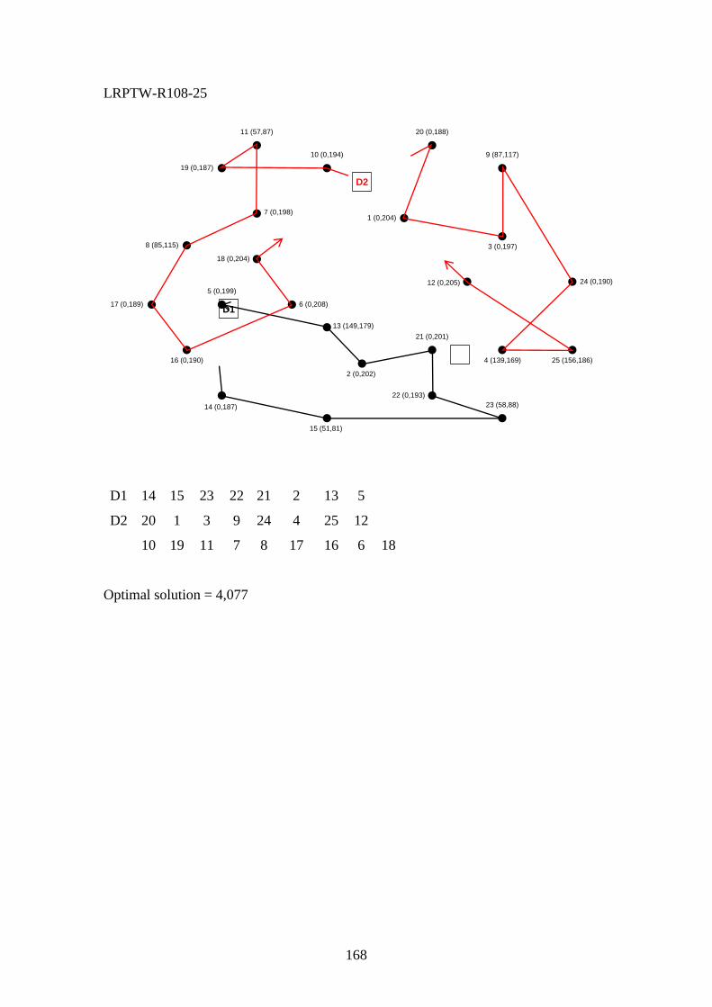
168
LRPTW-R108-25
D1 14 15 23 22 21 2 13 5
D2 20 1 3 9 24 4 25 12
10 19 11 7 8 17 16 6 18
Optimal solution = 4,077
1 (0,204)
2 (0,202)
3 (0,197)
4 (139,169)
5 (0,199)
6 (0,208)
7 (0,198)
8 (85,115)
9 (87,117)10 (0,194)
11 (57,87)
12 (0,205)
13 (149,179)
14 (0,187)
15 (51,81)
16 (0,190)
17 (0,189)
18 (0,204)
19 (0,187)
20 (0,188)
21 (0,201)
22 (0,193)
23 (58,88)
24 (0,190)
25 (156,186)
D1
D2
D3
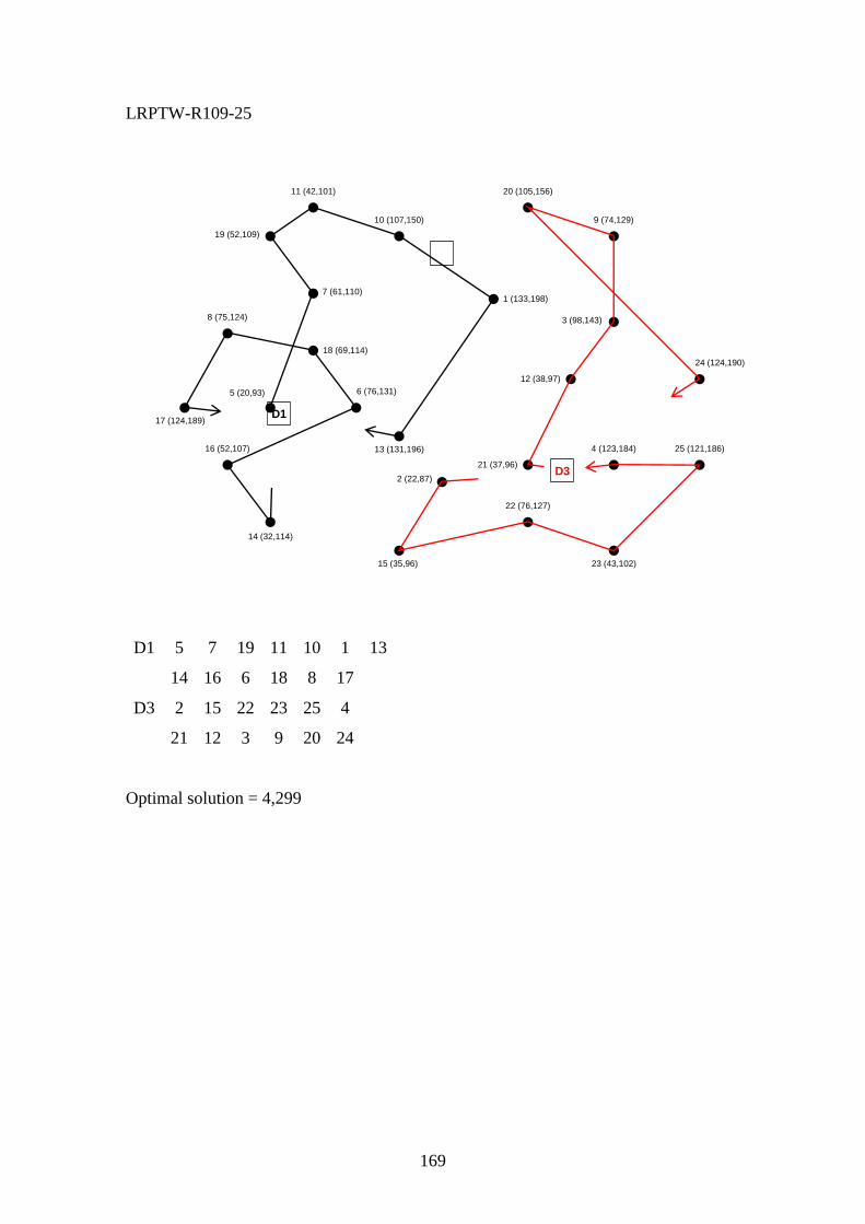
169
LRPTW-R109-25
D1 5 7 19 11 10 1 13
14 16 6 18 8 17
D3 2 15 22 23 25 4
21 12 3 9 20 24
Optimal solution = 4,299
1 (133,198)
2 (22,87)
3 (98,143)
4 (123,184)
5 (20,93) 6 (76,131)
7 (61,110)
8 (75,124)
9 (74,129)10 (107,150)
11 (42,101)
12 (38,97)
13 (131,196)
14 (32,114)
15 (35,96)
16 (52,107)
17 (124,189)
18 (69,114)
19 (52,109)
20 (105,156)
21 (37,96)
22 (76,127)
23 (43,102)
24 (124,190)
25 (121,186)
D1
D2
D3
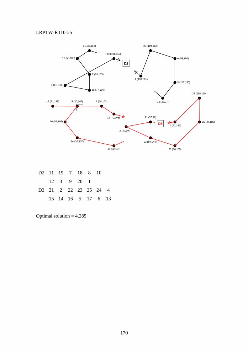
170
LRPTW-R110-25
D2 11 19 7 18 8 10
12 3 9 20 1
D3 21 2 22 23 25 24 4
15 14 16 5 17 6 13
Optimal solution = 4,285
1 (130,201)
2 (20,89)
3 (106,135)
4 (71,195)
5 (20,107) 6 (54,153)
7 (66,105)
8 (61,138)
9 (53,150)
10 (101,156)
11 (33,152)
12 (38,97)
13 (70,208)
14 (32,137)
15 (30,154)
16 (54,105)
17 (51,189)
18 (77,106)
19 (53,108)
20 (109,152)
21 (37,96)
22 (59,144)
23 (36,155)
24 (118,190)
25 (47,186)
D1
D2
D3
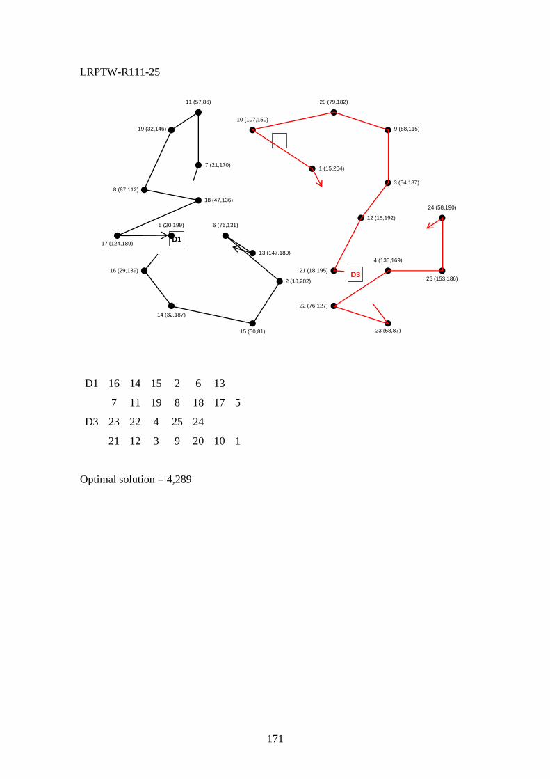
171
LRPTW-R111-25
D1 16 14 15 2 6 13
7 11 19 8 18 17 5
D3 23 22 4 25 24
21 12 3 9 20 10 1
Optimal solution = 4,289
1 (15,204)
2 (18,202)
3 (54,187)
4 (138,169)
5 (20,199) 6 (76,131)
7 (21,170)
8 (87,112)
9 (88,115)
10 (107,150)
11 (57,86)
12 (15,192)
13 (147,180)
14 (32,187)
15 (50,81)
16 (29,139)
17 (124,189)
18 (47,136)
19 (32,146)
20 (79,182)
21 (18,195)
22 (76,127)
23 (58,87)
24 (58,190)
25 (153,186)
D1
D2
D3

172
LRPTW-R112-25
D1 16 14 15 2 13 6
5 18 7 11 19 8 17
D3 21 22 23 25 4
12 24 3 9 20 10 1
Optimal solution = 4,250
1 (73,204)
2 (18,147)
3 (76,165)
4 (73,195)
5 (20,167) 6 (49,158)
7 (36,135)
8 (50,149)
9 (47,156)
10 (85,172)
11 (33,152)
12 (15,133)
13 (79,208)
14 (32,187)
15 (30,152)
16 (29,139)
17 (60,189)
18 (47,136)
19 (32,146)
20 (79,182)
21 (18,136)
22 (50,153)
23 (36,155)
24 (58,190)
25 (56,186)
D1
D2
D3
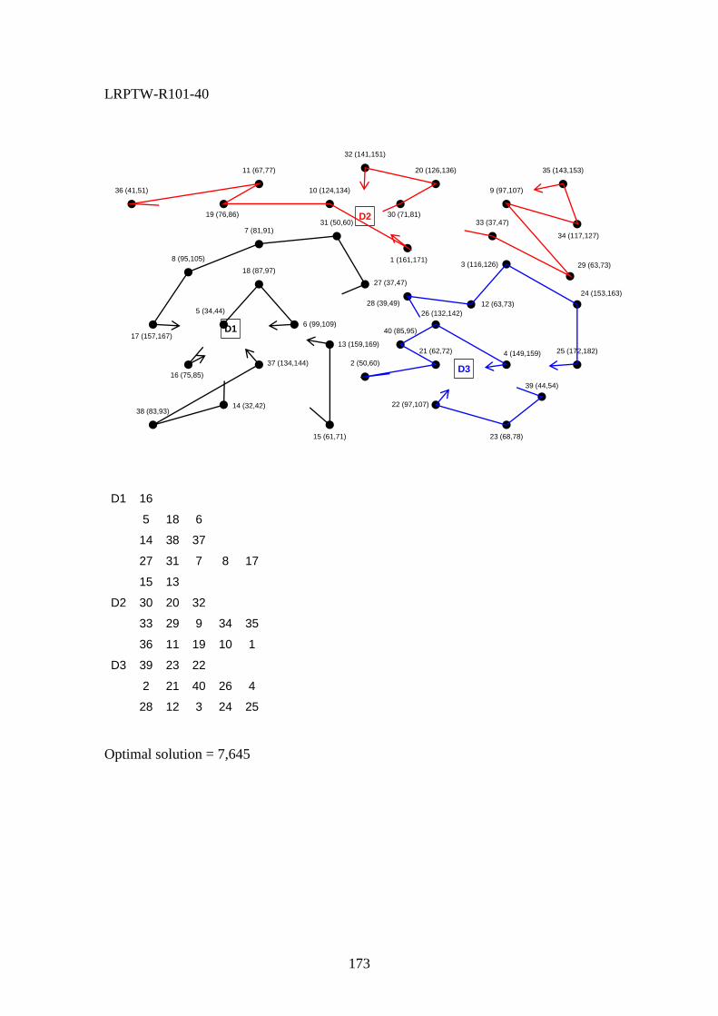
173
LRPTW-R101-40
D1 16
5 18 6
14 38 37
27 31 7 8 17
15 13
D2 30 20 32
33 29 9 34 35
36 11 19 10 1
D3 39 23 22
2 21 40 26 4
28 12 3 24 25
Optimal solution = 7,645
1 (161,171)
2 (50,60)
3 (116,126)
4 (149,159)
5 (34,44)
6 (99,109)
7 (81,91)
8 (95,105)
9 (97,107)10 (124,134)
11 (67,77)
12 (63,73)
13 (159,169)
14 (32,42)
15 (61,71)
16 (75,85)
17 (157,167)
18 (87,97)
19 (76,86)
20 (126,136)
21 (62,72)
22 (97,107)
23 (68,78)
24 (153,163)
25 (172,182)
26 (132,142)
27 (37,47)
28 (39,49)
29 (63,73)
30 (71,81)31 (50,60)
32 (141,151)
33 (37,47)
34 (117,127)
35 (143,153)
36 (41,51)
37 (134,144)
38 (83,93)
39 (44,54)
40 (85,95)D1
D2
D3
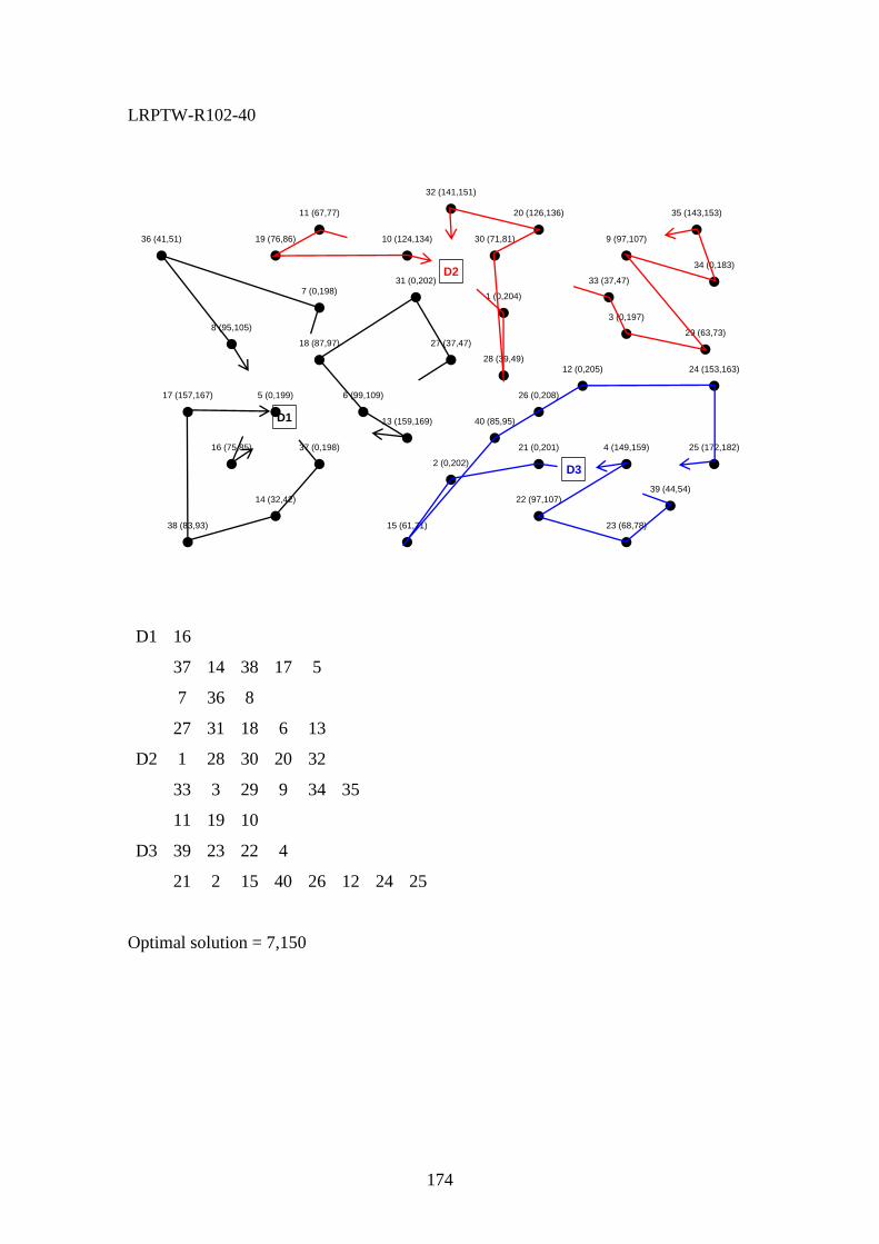
174
LRPTW-R102-40
D1 16
37 14 38 17 5
7 36 8
27 31 18 6 13
D2 1 28 30 20 32
33 3 29 9 34 35
11 19 10
D3 39 23 22 4
21 2 15 40 26 12 24 25
Optimal solution = 7,150
1 (0,204)
2 (0,202)
3 (0,197)
4 (149,159)
5 (0,199) 6 (99,109)
7 (0,198)
8 (95,105)
9 (97,107)10 (124,134)
11 (67,77)
12 (0,205)
13 (159,169)
14 (32,42)
15 (61,71)
16 (75,85)
17 (157,167)
18 (87,97)
19 (76,86)
20 (126,136)
21 (0,201)
22 (97,107)
23 (68,78)
24 (153,163)
25 (172,182)
26 (0,208)
27 (37,47)
28 (39,49)
29 (63,73)
30 (71,81)
31 (0,202)
32 (141,151)
33 (37,47)
34 (0,183)
35 (143,153)
36 (41,51)
37 (0,198)
38 (83,93)
39 (44,54)
40 (85,95)D1
D2
D3

175
Appendix C
Location of Depots and Shelters
in Ishinomaki

176
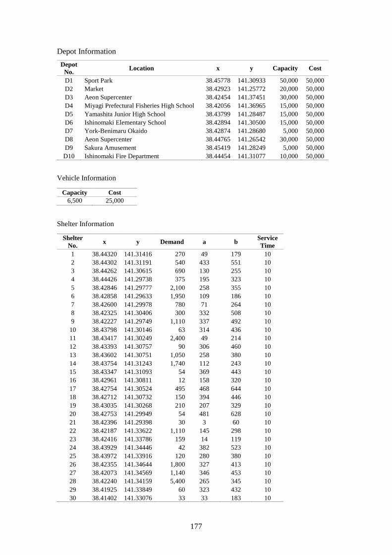
177
Depot Information
Depot
No. Location x y Capacity Cost
D1 Sport Park 38.45778 141.30933 50,000 50,000
D2 Market 38.42923 141.25772 20,000 50,000
D3 Aeon Supercenter 38.42454 141.37451 30,000 50,000
D4 Miyagi Prefectural Fisheries High School 38.42056 141.36965 15,000 50,000
D5 Yamashita Junior High School 38.43799 141.28487 15,000 50,000
D6 Ishinomaki Elementary School 38.42894 141.30500 15,000 50,000
D7 York-Benimaru Okaido 38.42874 141.28680 5,000 50,000
D8 Aeon Supercenter 38.44765 141.26542 30,000 50,000
D9 Sakura Amusement 38.45419 141.28249 5,000 50,000
D10 Ishinomaki Fire Department 38.44454 141.31077 10,000 50,000
Vehicle Information
Capacity Cost
6,500 25,000
Shelter Information
Shelter
No. x y Demand a b
Service
Time
1 38.44320 141.31416 270 49 179 10
2 38.44302 141.31191 540 433 551 10
3 38.44262 141.30615 690 130 255 10
4 38.44426 141.29738 375 195 323 10
5 38.42846 141.29777 2,100 258 355 10
6 38.42858 141.29633 1,950 109 186 10
7 38.42600 141.29978 780 71 264 10
8 38.42325 141.30406 300 332 508 10
9 38.42227 141.29749 1,110 337 492 10
10 38.43798 141.30146 63 314 436 10
11 38.43417 141.30249 2,400 49 214 10
12 38.43393 141.30757 90 306 460 10
13 38.43602 141.30751 1,050 258 380 10
14 38.43754 141.31243 1,740 112 243 10
15 38.43347 141.31093 54 369 443 10
16 38.42961 141.30811 12 158 320 10
17 38.42754 141.30524 495 468 644 10
18 38.42712 141.30732 150 394 446 10
19 38.43035 141.30268 210 207 329 10
20 38.42753 141.29949 54 481 628 10
21 38.42396 141.29398 30 3 60 10
22 38.42187 141.33622 1,110 145 298 10
23 38.42416 141.33786 159 14 119 10
24 38.43929 141.34446 42 382 523 10
25 38.43972 141.33916 120 280 380 10
26 38.42355 141.34644 1,800 327 413 10
27 38.42073 141.34569 1,140 346 453 10
28 38.42240 141.34159 5,400 265 345 10
29 38.41925 141.33849 60 323 432 10
30 38.41402 141.33076 33 33 183 10
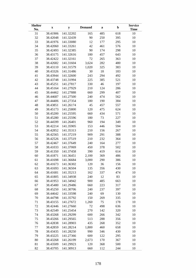
178
Shelter
No. x y Demand a b
Service
Time
31 38.41906 141.32202 165 485 618 10
32 38.42048 141.32439 90 250 395 10
33 38.41976 141.33080 12 177 295 10
34 38.42060 141.33261 42 461 576 10
35 38.42493 141.32385 90 174 298 10
36 38.43175 141.32616 180 457 643 10
37 38.42422 141.32161 72 265 363 10
38 38.42682 141.31604 3,624 282 480 10
39 38.43110 141.31579 1,020 325 383 10
40 38.43326 141.31486 30 18 183 10
41 38.43944 141.32600 243 294 492 10
42 38.43748 141.31994 225 385 521 10
43 38.45251 141.27817 330 46 197 10
44 38.45164 141.27929 210 124 286 10
45 38.44462 141.27888 660 299 407 10
46 38.44687 141.27500 240 474 562 10
47 38.44406 141.27354 180 190 384 10
48 38.43851 141.26174 45 457 557 10
49 38.45173 141.25800 120 475 624 10
50 38.45200 141.25595 660 434 571 10
51 38.45280 141.25596 180 73 227 10
52 38.44599 141.26401 960 194 349 10
53 38.42214 141.35905 153 446 594 10
54 38.42852 141.35313 210 156 267 10
55 38.42565 141.37219 909 291 388 10
56 38.42526 141.37519 210 232 364 10
57 38.42467 141.37649 240 164 277 10
58 38.41033 141.37069 450 378 502 10
59 38.41350 141.37458 390 419 614 10
60 38.41871 141.36451 2,100 369 486 10
61 38.41698 141.36684 3,000 290 386 10
62 38.41673 141.36302 120 36 156 10
63 38.41693 141.36504 135 356 430 10
64 38.41681 141.35213 162 337 474 10
65 38.41805 141.34938 240 12 83 10
66 38.41953 141.34942 900 485 663 10
67 38.45480 141.29486 660 223 317 10
68 38.45250 141.30706 240 237 397 10
69 38.44642 141.33598 240 69 130 10
70 38.44798 141.35792 150 269 335 10
71 38.43155 141.27672 1,260 75 178 10
72 38.42446 141.27660 72 498 636 10
73 38.42549 141.25454 270 142 320 10
74 38.43268 141.29299 600 266 342 10
75 38.43266 141.29565 513 288 356 10
76 38.42838 141.28903 435 268 352 10
77 38.42859 141.28214 1,800 460 658 10
78 38.43435 141.28250 990 346 430 10
79 38.43225 141.27366 600 122 295 10
80 38.43268 141.26199 2,673 170 367 10
81 38.43509 141.29923 120 368 500 10
82 38.43705 141.30913 660 112 244 10
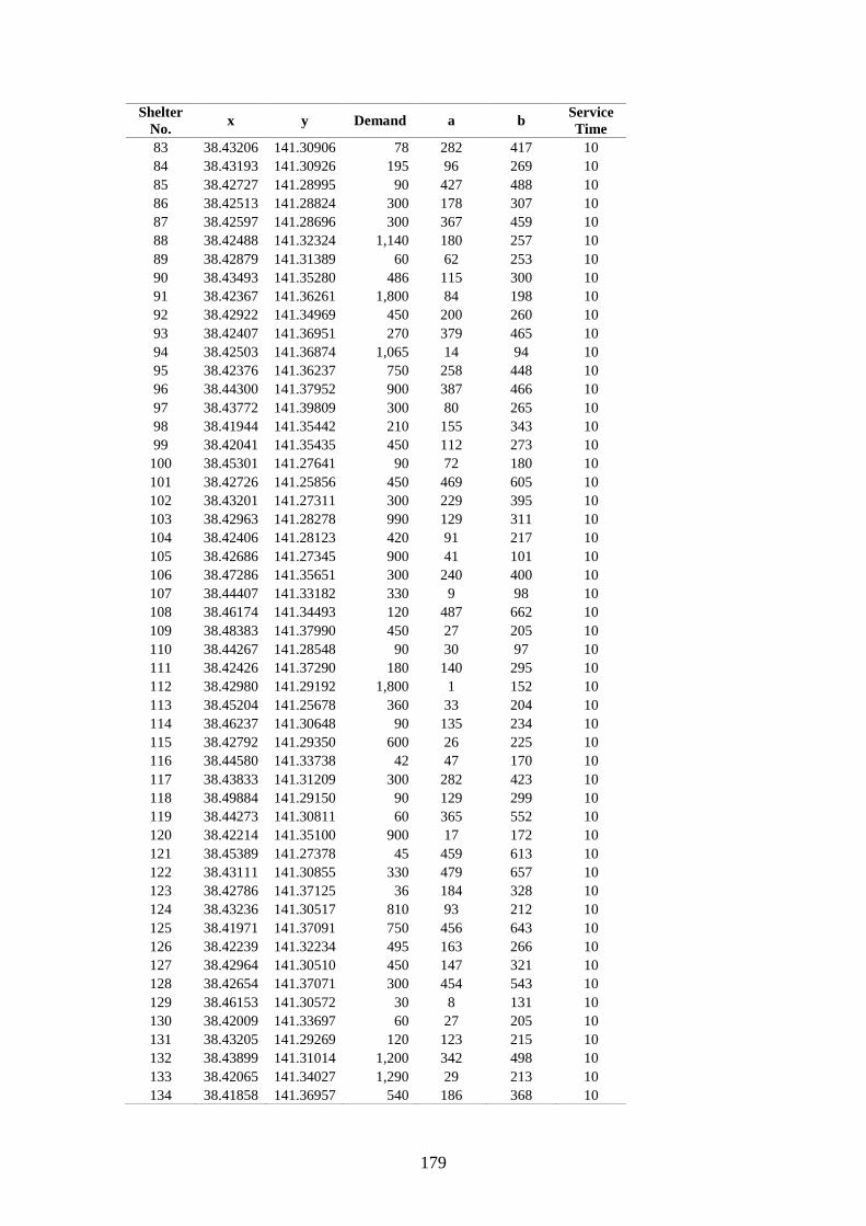
179
Shelter
No. x y Demand a b
Service
Time
83 38.43206 141.30906 78 282 417 10
84 38.43193 141.30926 195 96 269 10
85 38.42727 141.28995 90 427 488 10
86 38.42513 141.28824 300 178 307 10
87 38.42597 141.28696 300 367 459 10
88 38.42488 141.32324 1,140 180 257 10
89 38.42879 141.31389 60 62 253 10
90 38.43493 141.35280 486 115 300 10
91 38.42367 141.36261 1,800 84 198 10
92 38.42922 141.34969 450 200 260 10
93 38.42407 141.36951 270 379 465 10
94 38.42503 141.36874 1,065 14 94 10
95 38.42376 141.36237 750 258 448 10
96 38.44300 141.37952 900 387 466 10
97 38.43772 141.39809 300 80 265 10
98 38.41944 141.35442 210 155 343 10
99 38.42041 141.35435 450 112 273 10
100 38.45301 141.27641 90 72 180 10
101 38.42726 141.25856 450 469 605 10
102 38.43201 141.27311 300 229 395 10
103 38.42963 141.28278 990 129 311 10
104 38.42406 141.28123 420 91 217 10
105 38.42686 141.27345 900 41 101 10
106 38.47286 141.35651 300 240 400 10
107 38.44407 141.33182 330 9 98 10
108 38.46174 141.34493 120 487 662 10
109 38.48383 141.37990 450 27 205 10
110 38.44267 141.28548 90 30 97 10
111 38.42426 141.37290 180 140 295 10
112 38.42980 141.29192 1,800 1 152 10
113 38.45204 141.25678 360 33 204 10
114 38.46237 141.30648 90 135 234 10
115 38.42792 141.29350 600 26 225 10
116 38.44580 141.33738 42 47 170 10
117 38.43833 141.31209 300 282 423 10
118 38.49884 141.29150 90 129 299 10
119 38.44273 141.30811 60 365 552 10
120 38.42214 141.35100 900 17 172 10
121 38.45389 141.27378 45 459 613 10
122 38.43111 141.30855 330 479 657 10
123 38.42786 141.37125 36 184 328 10
124 38.43236 141.30517 810 93 212 10
125 38.41971 141.37091 750 456 643 10
126 38.42239 141.32234 495 163 266 10
127 38.42964 141.30510 450 147 321 10
128 38.42654 141.37071 300 454 543 10
129 38.46153 141.30572 30 8 131 10
130 38.42009 141.33697 60 27 205 10
131 38.43205 141.29269 120 123 215 10
132 38.43899 141.31014 1,200 342 498 10
133 38.42065 141.34027 1,290 29 213 10
134 38.41858 141.36957 540 186 368 10
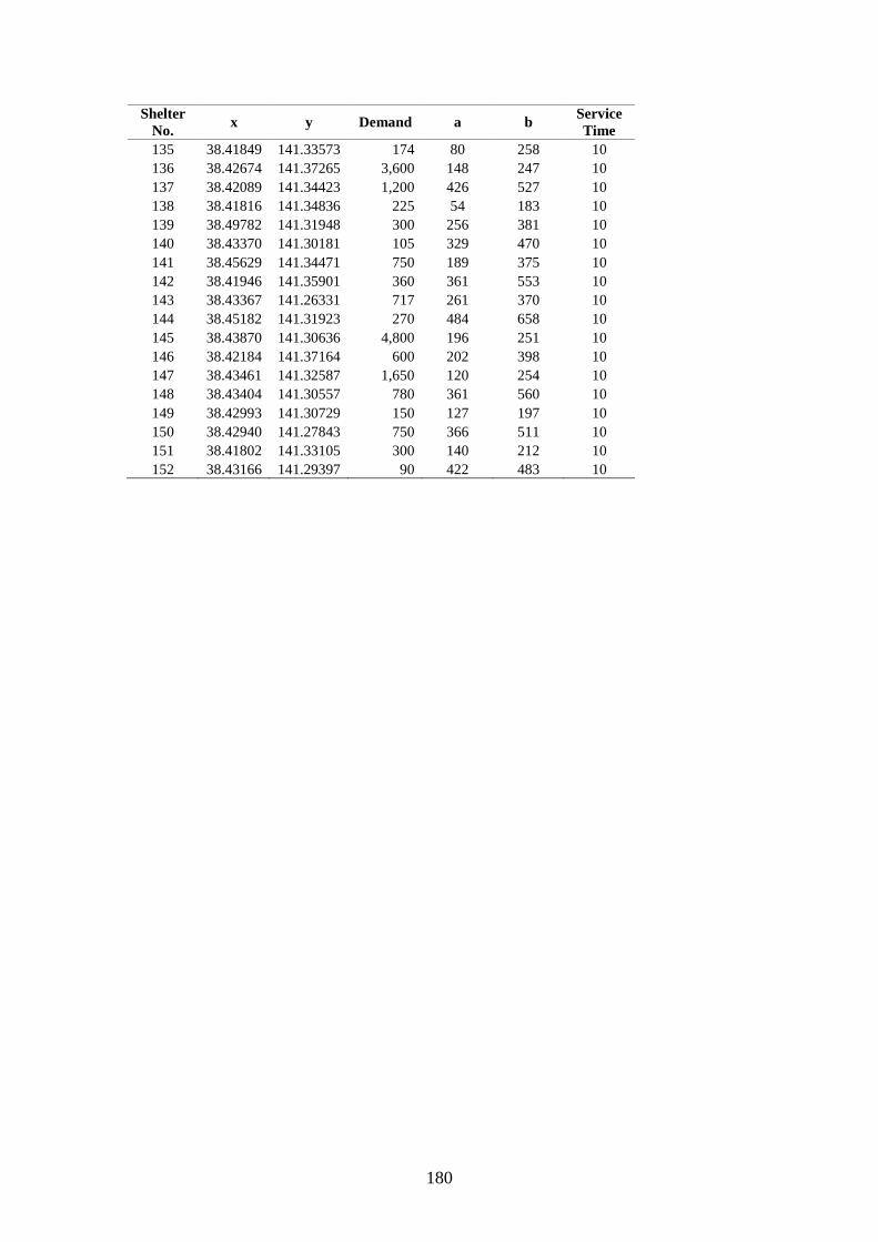
180
Shelter
No. x y Demand a b
Service
Time
135 38.41849 141.33573 174 80 258 10
136 38.42674 141.37265 3,600 148 247 10
137 38.42089 141.34423 1,200 426 527 10
138 38.41816 141.34836 225 54 183 10
139 38.49782 141.31948 300 256 381 10
140 38.43370 141.30181 105 329 470 10
141 38.45629 141.34471 750 189 375 10
142 38.41946 141.35901 360 361 553 10
143 38.43367 141.26331 717 261 370 10
144 38.45182 141.31923 270 484 658 10
145 38.43870 141.30636 4,800 196 251 10
146 38.42184 141.37164 600 202 398 10
147 38.43461 141.32587 1,650 120 254 10
148 38.43404 141.30557 780 361 560 10
149 38.42993 141.30729 150 127 197 10
150 38.42940 141.27843 750 366 511 10
151 38.41802 141.33105 300 140 212 10
152 38.43166 141.29397 90 422 483 10