EXACTLY SOLVABLE Q-EXTENDED NONLINEARCLASSICAL AND QUANTUM MODELS

A Thesis Submitted tothe Graduate School of Engineering and Sciences of

Izmir Institute of Technologyin Partial Fulfillment of the Requirements for the Degree of

MASTER OF SCIENCE

in Mathematics

bySengul NALCI

June 2011IZMIR

We approve the thesis of Sengul NALCI

Prof. Dr. Oktay PASHAEVSupervisor

Prof. Dr. Ismail Hakkı DURUCommittee Member

Prof. Dr. Ugur TIRNAKLICommittee Member

17 June 2011

Prof. Dr. Oguz YILMAZ Prof. Dr. Durmus Ali DEMIRHead of the Department of Dean of the Graduate School ofMathematics Engineering and Sciences

ACKNOWLEDGMENTS

I would like to express my deepest gratitude to my advisor, Prof. Dr. Oktay

Pashaev, for his academic guidance, motivating talks, help and patience throughout my

graduate education, especially during preparation of this thesis. I sincerely thank Prof.

Dr. Ugur Tırnaklı for being a member of my thesis committee. I would like to thank

TUBITAK for graduate students scholarship, supporting my master programme studies.

I also want to thank my colleague and close friend, Neslihan Eti, for her encouragement,

support and help.

Finally, I am very grateful to my family for their support, understanding and love

during my education.

ABSTRACT

EXACTLY SOLVABLE Q-EXTENDED NONLINEAR CLASSICAL ANDQUANTUM MODELS

In the present thesis we study q-extended exactly solvable nonlinear classical and

quantum models. In these models the derivative operator is replaced by q-derivative, in

the form of finite difference dilatation operator. It requires introducing q-numbers instead

of standard numbers, and q-calculus instead of standard calculus. We start with classical

q-damped oscillator and q-difference heat equation. Exact solutions are constructed as

q-Hermite and Kampe-de Feriet polynomials and Jackson q-exponential functions. By

q-Cole-Hopf transformation we obtain q-nonlinear heat equation in the form of Burg-

ers equation. IVP for this equation is solved in operator form and q-shock soliton so-

lutions are found. Results are extended to linear q-Schrodinger equation and nonlinear

q-Maddelung fluid. Motivated by physical applications, then we introduce the multi-

ple q-calculus. In addition to non-symmetrical and symmetrical q-calculus it includes

the new Fibonacci calculus, based on Binet-Fibonacci formula. We show that multiple

q-calculus naturally appears in construction of Q-commutative q-binomial formula, gen-

eralizing all well-known formulas as Newton, Gauss, and noncommutative ones. As an-

other application we study quantum two parametric deformations of harmonic oscillator

and corresponding q-deformed quantum angular momentum. A new type of q-function

of two variables is introduced as q-holomorphic function, satisfying q-Cauchy-Riemann

equations. In spite of that q-holomorphic function is not analytic in the usual sense, it

represents the so-called generalized analytic function. The q-traveling waves as solutions

of q-wave equation are derived. To solve the q-BVP we introduce q-Bernoulli numbers,

and their relation with zeros of q-Sine function.

iv

OZET

TAM COZUMLENEBILEN DOGRUSAL OLMAYAN Q-GENISLETILMIS KLASIKVE KUANTUM MODELLERI

Bu tezde, tam cozumlenebilen dogrusal olmayan q-genisletilmis klasik ve kuan-

tum modelleri calısılmıstır. Modellerde turev operatoru sonlu fark dilasyon operator for-

munda tanımlanan q-turev operatoru ile degistirilmistir. Bu calısma, standart sayıların

q-sayıları ve standart hesaplamanın q-hesaplama ile degistirilmesini gerektirmistir. Ilk

olarak klasik q-sonumlu osilasyon modeli ve q-fark ısı denklemi ile calısıldı ve kesin

cozumleri q-Hermite ve Kampe-de Feriet polinomlar ve Jackson q-ustel fonksiyonlar

cinsinden bulundu. q-Cole-Hopf donusumu kullanılarak dogrusal olmayan q-ısı den-

klemi Burgers denklemi formunda elde edildi. Burgers denklemi icin baslangıc deger

problemini operator cinsinden cozduk ve q-sok soliton cozumleri bulduk. Elde edilen

sonuclar, dogrusal q-Schrodinger denklemi ve dogrusal olmayan q-Maddelung akıskanlar

icin genisletilmistir. Fiziksel uygulamalardan yola cıkarak coklu q-hesaplama tanımladık.

Bu coklu hesaplama simetrik ve simetrik olmayan q-hesaplamalara ek olarak, Binet-

Fibonacci formulune dayanan yeni Fibonacci hesaplamayı da icerir. Coklu q-hesaplama-

nın, bilinen Newton, Gauss ve degismeli olmayan binom formullerinin genel hali olan

Q-degismeli q-binom formulunun yapılandırılması sırasında ortaya cıktıgı gosterildi. Bu

hesaplamanın diger bir uygulaması olarak iki parametrik deformasyonlu kuantum har-

monik osilasyon modeli ve ilgili q-deforme olmus kuantum acısal momentum calısılmıstır.

q-Cauchy-Riemann denklemlerini saglayan iki degiskenli q-holomorfik olan yeni bir q-

fonksiyon tanıtılmıstır. q-holomorfik fonksiyon alısılmıs anlamda analitik olmamasına

ragmen genellestirilmis analitik fonksiyon olarak gosterildi. q-Dalga denkleminin cozumu

olan q-hareket eden dalgalar bulunmustur. q-Sınır deger problemini cozmek icin gerekli

olan q-Bernoulli sayıları ve bunların q-sinus fonksiyonunun sıfırları ile iliskisi hesap-

landı.

v

TABLE OF CONTENTS

LIST OF FIGURES . . . . . . . . . . . . . . . . . . . . . . . . . . . . . . . . . . . . . . . . . . . . . . . . . . . . . . . . . . . . . . . . . . . . . . . xi

LIST OF TABLES . . . . . . . . . . . . . . . . . . . . . . . . . . . . . . . . . . . . . . . . . . . . . . . . . . . . . . . . . . . . . . . . . . . . . . . . xiii

CHAPTER 1. INTRODUCTION . . . . . . . . . . . . . . . . . . . . . . . . . . . . . . . . . . . . . . . . . . . . . . . . . . . . . . . 1

CHAPTER 2. BASIC Q-CALCULUS . . . . . . . . . . . . . . . . . . . . . . . . . . . . . . . . . . . . . . . . . . . . . . . . . 6

2.1. q-Numbers . . . . . . . . . . . . . . . . . . . . . . . . . . . . . . . . . . . . . . . . . . . . . . . . . . . . . . . . . . . . . 6

2.1.1. Non-symmetrical q-Numbers . . . . . . . . . . . . . . . . . . . . . . . . . . . . . . . . . . . . . 6

2.1.2. Symmetrical q-Numbers . . . . . . . . . . . . . . . . . . . . . . . . . . . . . . . . . . . . . . . . . . 9

2.2. q-Derivative . . . . . . . . . . . . . . . . . . . . . . . . . . . . . . . . . . . . . . . . . . . . . . . . . . . . . . . . . . . . 9

2.3. q-Taylor’s Formula and Binomial Formulas . . . . . . . . . . . . . . . . . . . . . . . . . 11

2.4. q-Pascal Triangle . . . . . . . . . . . . . . . . . . . . . . . . . . . . . . . . . . . . . . . . . . . . . . . . . . . . . . 12

2.5. q-Integral . . . . . . . . . . . . . . . . . . . . . . . . . . . . . . . . . . . . . . . . . . . . . . . . . . . . . . . . . . . . . . . 13

2.6. q-Elementary Functions . . . . . . . . . . . . . . . . . . . . . . . . . . . . . . . . . . . . . . . . . . . . . . . 14

CHAPTER 3. Q-DAMPED OSCILLATOR . . . . . . . . . . . . . . . . . . . . . . . . . . . . . . . . . . . . . . . . . . . 17

3.1. Damped Oscillator . . . . . . . . . . . . . . . . . . . . . . . . . . . . . . . . . . . . . . . . . . . . . . . . . . . . 17

3.2. q-Harmonic Oscillator . . . . . . . . . . . . . . . . . . . . . . . . . . . . . . . . . . . . . . . . . . . . . . . . 18

3.3. q-Damped q-Harmonic Oscillator . . . . . . . . . . . . . . . . . . . . . . . . . . . . . . . . . . . . 20

3.3.1. Under-Damping Case . . . . . . . . . . . . . . . . . . . . . . . . . . . . . . . . . . . . . . . . . . . . . 21

3.3.2. Over-Damping Case . . . . . . . . . . . . . . . . . . . . . . . . . . . . . . . . . . . . . . . . . . . . . . . 21

3.3.3. Critical Case . . . . . . . . . . . . . . . . . . . . . . . . . . . . . . . . . . . . . . . . . . . . . . . . . . . . . . . 22

3.4. Degenerate Roots for Equation Degree N . . . . . . . . . . . . . . . . . . . . . . . . . . . . 26

CHAPTER 4. Q-SPACE-TIME DIFFERENCE HEAT EQUATION . . . . . . . . . . . . . . . . . 30

4.1. q-Hermite Polynomials . . . . . . . . . . . . . . . . . . . . . . . . . . . . . . . . . . . . . . . . . . . . . . . 30

4.1.1. q-Difference Equation . . . . . . . . . . . . . . . . . . . . . . . . . . . . . . . . . . . . . . . . . . . . . 33

4.2. Operator Representation . . . . . . . . . . . . . . . . . . . . . . . . . . . . . . . . . . . . . . . . . . . . . . 34

4.3. q- Kampe-de Feriet Polynomials . . . . . . . . . . . . . . . . . . . . . . . . . . . . . . . . . . . . . 35

4.4. q-Heat Equation . . . . . . . . . . . . . . . . . . . . . . . . . . . . . . . . . . . . . . . . . . . . . . . . . . . . . . . 36

4.5. Evolution Operator . . . . . . . . . . . . . . . . . . . . . . . . . . . . . . . . . . . . . . . . . . . . . . . . . . . . 37

vi

CHAPTER 5. Q-SPACE-TIME DIFFERENCE BURGERS’ EQUATION . . . . . . . . . . 39

5.1. Burger’s Equation and Cole-Hopf Transformation . . . . . . . . . . . . . . . . . 39

5.2. q-Burger’s Equation as nonlinear q-Heat Equation . . . . . . . . . . . . . . . . . . 39

5.2.1. I.V.P. for q-Burgers’ Type Equation . . . . . . . . . . . . . . . . . . . . . . . . . . . . . 40

5.3. q-Shock Soliton . . . . . . . . . . . . . . . . . . . . . . . . . . . . . . . . . . . . . . . . . . . . . . . . . . . . . . . 40

CHAPTER 6. Q-SPACE DIFFERENCE AND TIME DIFFERENTIAL HEAT

EQUATION . . . . . . . . . . . . . . . . . . . . . . . . . . . . . . . . . . . . . . . . . . . . . . . . . . . . . . . . . . . . . . 48

6.1. q-Hermite Polynomials . . . . . . . . . . . . . . . . . . . . . . . . . . . . . . . . . . . . . . . . . . . . . . . 48

6.1.1. q-Difference Equation . . . . . . . . . . . . . . . . . . . . . . . . . . . . . . . . . . . . . . . . . . . . . 51

6.2. q-Kampe-de Feriet Polynomials . . . . . . . . . . . . . . . . . . . . . . . . . . . . . . . . . . . . . . 52

6.3. q-Heat Equation . . . . . . . . . . . . . . . . . . . . . . . . . . . . . . . . . . . . . . . . . . . . . . . . . . . . . . . 53

6.3.1. Operator Representation . . . . . . . . . . . . . . . . . . . . . . . . . . . . . . . . . . . . . . . . . . 54

6.4. Evolution Operator . . . . . . . . . . . . . . . . . . . . . . . . . . . . . . . . . . . . . . . . . . . . . . . . . . . . 55

CHAPTER 7. Q-SPACE DIFFERENCE AND TIME DIFFERENTIAL BURGER’S

EQUATION . . . . . . . . . . . . . . . . . . . . . . . . . . . . . . . . . . . . . . . . . . . . . . . . . . . . . . . . . . . . . . 57

7.1. q-Cole-Hopf Transfomation and q-Burger’s Equation . . . . . . . . . . . . . . 57

7.1.1. I.V.P. for q-Burgers’ Type Equation . . . . . . . . . . . . . . . . . . . . . . . . . . . . . 57

7.2. q-Shock Soliton . . . . . . . . . . . . . . . . . . . . . . . . . . . . . . . . . . . . . . . . . . . . . . . . . . . . . . . 58

CHAPTER 8. Q-SCHRODINGER EQUATION AND Q-MADDELUNG FLUID . 65

8.1. Standard Time-Dependent q-Schrodinger Equation . . . . . . . . . . . . . . . . . 65

CHAPTER 9. MULTIPLE Q-CALCULUS . . . . . . . . . . . . . . . . . . . . . . . . . . . . . . . . . . . . . . . . . . . . 68

9.1. Multiple q- Numbers . . . . . . . . . . . . . . . . . . . . . . . . . . . . . . . . . . . . . . . . . . . . . . . . . . 68

9.1.1. Multiple q-Derivative . . . . . . . . . . . . . . . . . . . . . . . . . . . . . . . . . . . . . . . . . . . . . 70

9.1.2. N = 1 Case . . . . . . . . . . . . . . . . . . . . . . . . . . . . . . . . . . . . . . . . . . . . . . . . . . . . . . . . . 71

9.1.3. N = 2 Cases . . . . . . . . . . . . . . . . . . . . . . . . . . . . . . . . . . . . . . . . . . . . . . . . . . . . . . . . 71

9.1.3.1. Non-symmetrical Case . . . . . . . . . . . . . . . . . . . . . . . . . . . . . . . . . . . . . 71

9.1.3.2. Symmetrical Case . . . . . . . . . . . . . . . . . . . . . . . . . . . . . . . . . . . . . . . . . . . 72

9.1.3.3. Fibonacci Case . . . . . . . . . . . . . . . . . . . . . . . . . . . . . . . . . . . . . . . . . . . . . . 72

9.1.3.4. Symmetrical Golden Case . . . . . . . . . . . . . . . . . . . . . . . . . . . . . . . . . . 73

9.1.4. q-Leibnitz Rule . . . . . . . . . . . . . . . . . . . . . . . . . . . . . . . . . . . . . . . . . . . . . . . . . . . . 74

9.1.5. Generalized Taylor Formula . . . . . . . . . . . . . . . . . . . . . . . . . . . . . . . . . . . . . . 75

vii

9.1.6. q-Polynomial Expansion . . . . . . . . . . . . . . . . . . . . . . . . . . . . . . . . . . . . . . . . . . 80

9.1.7. Multiple q-Binomial Formula . . . . . . . . . . . . . . . . . . . . . . . . . . . . . . . . . . . . 81

9.2. q-Multiple Pascal Triangle . . . . . . . . . . . . . . . . . . . . . . . . . . . . . . . . . . . . . . . . . . . . 86

9.3. q-Multiple Antiderivative . . . . . . . . . . . . . . . . . . . . . . . . . . . . . . . . . . . . . . . . . . . . . 87

9.3.1. q-Periodic Functions and Euler Equation . . . . . . . . . . . . . . . . . . . . . . . . 89

9.4. q-Multiple Jackson Integral . . . . . . . . . . . . . . . . . . . . . . . . . . . . . . . . . . . . . . . . . . . 90

CHAPTER 10. NON-COMMUTATIVE Q-BINOMIAL FORMULAS . . . . . . . . . . . . . . . 92

10.1. Gauss’s Binomial Formula . . . . . . . . . . . . . . . . . . . . . . . . . . . . . . . . . . . . . . . . . . . . 92

10.2. Non-commutative Binomial Formula . . . . . . . . . . . . . . . . . . . . . . . . . . . . . . . . 95

10.3. Q-commutative q-Binomial Formula . . . . . . . . . . . . . . . . . . . . . . . . . . . . . . . . . 96

10.3.1. Special Cases . . . . . . . . . . . . . . . . . . . . . . . . . . . . . . . . . . . . . . . . . . . . . . . . . . . . . . 106

10.3.2. q, Q- Binomial Formula . . . . . . . . . . . . . . . . . . . . . . . . . . . . . . . . . . . . . . . . . . . 107

10.3.3. q-Function of Non-commutative Variables . . . . . . . . . . . . . . . . . . . . . . 107

CHAPTER 11. Q-QUANTUM HARMONIC OSCILLATOR . . . . . . . . . . . . . . . . . . . . . . . . . 110

11.1. Quantum Harmonic Oscillator . . . . . . . . . . . . . . . . . . . . . . . . . . . . . . . . . . . . . . . . 110

11.2. (qi, qj)-Quantum Harmonic Oscillator . . . . . . . . . . . . . . . . . . . . . . . . . . . . . . . 114

11.2.1. Binet-Fibonacci Golden Oscillator and Fibonacci Sequence . . . 124

11.2.2. Symmetrical q-Oscillator . . . . . . . . . . . . . . . . . . . . . . . . . . . . . . . . . . . . . . . . . 128

11.2.3. Non-symmetrical q-Oscillator . . . . . . . . . . . . . . . . . . . . . . . . . . . . . . . . . . . . 131

11.3. q-Deformed Quantum Angular Momentum . . . . . . . . . . . . . . . . . . . . . . . . . . 132

11.3.1. Double q-Boson Algebra Representation . . . . . . . . . . . . . . . . . . . . . . . . 132

11.3.2. su(qi,qj)(2) Angular Momentum Algebra . . . . . . . . . . . . . . . . . . . . . . . . 136

11.3.3. Double Boson Representation of su(qi,qj)(2) Angular

Momentum . . . . . . . . . . . . . . . . . . . . . . . . . . . . . . . . . . . . . . . . . . . . . . . . . . . . . . . . 141

11.3.3.1. Non-symmetrical Case: . . . . . . . . . . . . . . . . . . . . . . . . . . . . . . . . . . . . . 143

11.3.3.2. Symmetrical Case: . . . . . . . . . . . . . . . . . . . . . . . . . . . . . . . . . . . . . . . . . . 144

11.3.3.3. Binet-Fibonacci Case: . . . . . . . . . . . . . . . . . . . . . . . . . . . . . . . . . . . . . . 144

11.3.4. su√qjqi

(2) case: . . . . . . . . . . . . . . . . . . . . . . . . . . . . . . . . . . . . . . . . . . . . . . . . . . . . 147

11.3.4.1. Complex Symmetrical su(iϕ, iϕ

)(2) Quantum Algebra . . . . 148

11.3.5. su(qi,qj)(2) Case: . . . . . . . . . . . . . . . . . . . . . . . . . . . . . . . . . . . . . . . . . . . . . . . . . . . 149

11.3.5.1. suF (2) Algebra . . . . . . . . . . . . . . . . . . . . . . . . . . . . . . . . . . . . . . . . . . . . . 150

viii

CHAPTER 12. Q-FUNCTION OF ONE VARIABLE . . . . . . . . . . . . . . . . . . . . . . . . . . . . . . . . . 151

12.1. q-Function of One Variable . . . . . . . . . . . . . . . . . . . . . . . . . . . . . . . . . . . . . . . . . . . 152

12.1.1. Addition Formulas . . . . . . . . . . . . . . . . . . . . . . . . . . . . . . . . . . . . . . . . . . . . . . . . 157

12.2. Complex Analytic Function . . . . . . . . . . . . . . . . . . . . . . . . . . . . . . . . . . . . . . . . . . 162

12.3. q-Holomorphic Function . . . . . . . . . . . . . . . . . . . . . . . . . . . . . . . . . . . . . . . . . . . . . . 163

12.3.1. q-Analytic Function . . . . . . . . . . . . . . . . . . . . . . . . . . . . . . . . . . . . . . . . . . . . . . . 165

12.3.2. q-Cauchy-Riemann Equations . . . . . . . . . . . . . . . . . . . . . . . . . . . . . . . . . . . . 166

12.3.3. q-Analytic Function as Generalized Analytic Function . . . . . . . . . 167

12.4. Traveling Wave . . . . . . . . . . . . . . . . . . . . . . . . . . . . . . . . . . . . . . . . . . . . . . . . . . . . . . . . 169

12.5. q-Traveling Wave . . . . . . . . . . . . . . . . . . . . . . . . . . . . . . . . . . . . . . . . . . . . . . . . . . . . . . 170

12.6. D’Alembert Solution of Wave Equation . . . . . . . . . . . . . . . . . . . . . . . . . . . . . 171

12.7. The q-Wave Equation . . . . . . . . . . . . . . . . . . . . . . . . . . . . . . . . . . . . . . . . . . . . . . . . . 172

12.7.1. D’Alembert Solution of The q-Wave Equation . . . . . . . . . . . . . . . . . . 176

12.7.2. Initial Boundary Value Problem for q-Wave Equation . . . . . . . . . . 182

12.8. q-Bernoulli Numbers and Zeros of q-Sine Function . . . . . . . . . . . . . . . . . 188

12.8.1. Zeros of Sine Function and Riemann Zeta Function . . . . . . . . . . . . 189

12.8.2. q-Bernoulli Polynomials and Numbers . . . . . . . . . . . . . . . . . . . . . . . . . . . 193

12.8.3. q-Schrodinger Equation for a Particle in a Potential Well . . . . . . . 201

CHAPTER 13. CONCLUSION . . . . . . . . . . . . . . . . . . . . . . . . . . . . . . . . . . . . . . . . . . . . . . . . . . . . . . . . . . 205

REFERENCES . . . . . . . . . . . . . . . . . . . . . . . . . . . . . . . . . . . . . . . . . . . . . . . . . . . . . . . . . . . . . . . . . . . . . . . . . . . 207

APPENDICES . . . . . . . . . . . . . . . . . . . . . . . . . . . . . . . . . . . . . . . . . . . . . . . . . . . . . . . . . . . . . . . . . . . . . . . . . . . . 214

APPENDIX A. CONSTANT COEFFICIENT Q-DIFFERENCE EQUATION . . . . . . 214

APPENDIX B. MULTIPLE Q-POLYNOMIALS . . . . . . . . . . . . . . . . . . . . . . . . . . . . . . . . . . . . . . 218

APPENDIX C. Q-BINOMIAL FORMULAS . . . . . . . . . . . . . . . . . . . . . . . . . . . . . . . . . . . . . . . . . . 223

APPENDIX D. Q-QUANTUM HARMONIC OSCILLATOR . . . . . . . . . . . . . . . . . . . . . . . . 226

APPENDIX E. QUANTUM ANGULAR MOMENTUM REPRESENTATION . . . . 230

APPENDIX F. Q-QUANTUM ANGULAR MOMENTUM . . . . . . . . . . . . . . . . . . . . . . . . . . 232

APPENDIX G. Q-FUNCTION OF ONE VARIABLE . . . . . . . . . . . . . . . . . . . . . . . . . . . . . . . . 235

APPENDIX H. Q-TRAVELING WAVE . . . . . . . . . . . . . . . . . . . . . . . . . . . . . . . . . . . . . . . . . . . . . . . . 237

APPENDIX I. Q-BERNOULLI NUMBERS BQ2 AND BQ

4 . . . . . . . . . . . . . . . . . . . . . . . . . . 241

APPENDIX J. ZEROS OF SINQ X FUNCTION . . . . . . . . . . . . . . . . . . . . . . . . . . . . . . . . . . . . . 243

ix

LIST OF FIGURES

Figure Page

Figure 2.1. Conformal mapping of complex q-number z . . . . . . . . . . . . . . . . . . . . . . . . . . . . . . 8

Figure 2.2. q-Pascal Triangle . . . . . . . . . . . . . . . . . . . . . . . . . . . . . . . . . . . . . . . . . . . . . . . . . . . . . . . . . . . . 13

Figure 3.1. q-Harmonic oscillator solution cosq t . . . . . . . . . . . . . . . . . . . . . . . . . . . . . . . . . . . . . . 19

Figure 3.2. q-Harmonic oscillator solution sin(

2πln q

ln t)

cosq t . . . . . . . . . . . . . . . . . . . . . . . 20

Figure 3.3. Under-damping case A = B = 1 . . . . . . . . . . . . . . . . . . . . . . . . . . . . . . . . . . . . . . . . . . . 22

Figure 3.4. Under-damping case with q-periodic function . . . . . . . . . . . . . . . . . . . . . . . . . . . . . 22

Figure 3.5. Over-damping case A = B = 1 . . . . . . . . . . . . . . . . . . . . . . . . . . . . . . . . . . . . . . . . . . . . 23

Figure 3.6. Over-damping case with q-periodic function . . . . . . . . . . . . . . . . . . . . . . . . . . . . . . 24

Figure 3.7. Critical case . . . . . . . . . . . . . . . . . . . . . . . . . . . . . . . . . . . . . . . . . . . . . . . . . . . . . . . . . . . . . . . . . 25

Figure 3.8. Critical case with periodic function . . . . . . . . . . . . . . . . . . . . . . . . . . . . . . . . . . . . . . . . 25

Figure 3.9. Self-similar micro structure at scale 0.5 . . . . . . . . . . . . . . . . . . . . . . . . . . . . . . . . . . . 26

Figure 3.10. Self-similar micro structure at scale 0.05 . . . . . . . . . . . . . . . . . . . . . . . . . . . . . . . . . . 27

Figure 5.1. Singular q-shock soliton . . . . . . . . . . . . . . . . . . . . . . . . . . . . . . . . . . . . . . . . . . . . . . . . . . . . 42

Figure 5.2. The regular q-shock soliton for k1 = 1, k2 = −1, at range (-50, 50) . . . . . 43

Figure 5.3. The regular q-shock soliton for k1 = 1, k2 = −1 at range (-5000, 5000) 44

Figure 5.4. The regular q-shock soliton for k1 = 1, k2 = −1 at range (-500000,

500000) . . . . . . . . . . . . . . . . . . . . . . . . . . . . . . . . . . . . . . . . . . . . . . . . . . . . . . . . . . . . . . . . . . . . . 44

Figure 5.5. q-Shock soliton . . . . . . . . . . . . . . . . . . . . . . . . . . . . . . . . . . . . . . . . . . . . . . . . . . . . . . . . . . . . . . 45

Figure 5.6. q-Shock soliton with q-periodic modulation . . . . . . . . . . . . . . . . . . . . . . . . . . . . . . . 45

Figure 5.7. Self-similar q-shock soliton micro structure at scale 0.3 . . . . . . . . . . . . . . . . . . 46

Figure 5.8. Self-similar q-shock soliton micro structure at scale 0.03 . . . . . . . . . . . . . . . . 46

Figure 5.9. Multi q-shock regular for k1 = 1, k2 = −1, k3 = 10, k4 = −10 at

t = 0 . . . . . . . . . . . . . . . . . . . . . . . . . . . . . . . . . . . . . . . . . . . . . . . . . . . . . . . . . . . . . . . . . . . . . . . . 47

Figure 7.1. q-Shock evolution for ν = 1, k1 = 1, k2 = −1, t = −2 at range (-50,

50) . . . . . . . . . . . . . . . . . . . . . . . . . . . . . . . . . . . . . . . . . . . . . . . . . . . . . . . . . . . . . . . . . . . . . . . . . . . . 60

Figure 7.2. q-Shock evolution for ν = 1, k1 = 1, k2 = −1, t = 0 at range (-50, 50) . 60

Figure 7.3. q-Shock evolution for ν = 1, k1 = 1, k2 = −1, t = 5 at range (-50, 50) . 61

Figure 7.4. 3D plot of q-shock evolution for k1 = 1, k2 = −1,k3 = 2, k4 = −2

and at range (-50, 50) . . . . . . . . . . . . . . . . . . . . . . . . . . . . . . . . . . . . . . . . . . . . . . . . . . . . . . . 62

Figure 7.5. Multi q-shock evolution for k1 = 1, k2 = −1,k3 = 2, k4 = −2,

t = −10 and at range (-50, 50) . . . . . . . . . . . . . . . . . . . . . . . . . . . . . . . . . . . . . . . . . . . . 63

x

Figure 7.6. Multi q-shock evolution for k1 = 1, k2 = −1,k3 = 2, k4 = −2, t = 0

and at range (-50, 50) . . . . . . . . . . . . . . . . . . . . . . . . . . . . . . . . . . . . . . . . . . . . . . . . . . . . . . . 63

Figure 7.7. Multi q-shock evolution for k1 = 1, k2 = −1,k3 = 2, k4 = −2, t = 7

and at range (-50, 50) . . . . . . . . . . . . . . . . . . . . . . . . . . . . . . . . . . . . . . . . . . . . . . . . . . . . . . . 64

Figure 7.8. 3D plot of multiple q-shock evolution for k1 = 1, k2 = −1,k3 = 2,

k4 = −2, and at range (-50, 50) . . . . . . . . . . . . . . . . . . . . . . . . . . . . . . . . . . . . . . . . . . . . 64

Figure 9.1. (qi, qj)-Pascal Triangle . . . . . . . . . . . . . . . . . . . . . . . . . . . . . . . . . . . . . . . . . . . . . . . . . . . . . . 87

Figure 10.1. Q-commutative q-Pascal triangle . . . . . . . . . . . . . . . . . . . . . . . . . . . . . . . . . . . . . . . . . . . 99

Figure 11.1. Fibonacci tree for spectrum of Golden Oscillator . . . . . . . . . . . . . . . . . . . . . . . . . 127

xi

LIST OF TABLES

Table Page

Table 12.1. Table of q-sine zeros . . . . . . . . . . . . . . . . . . . . . . . . . . . . . . . . . . . . . . . . . . . . . . . . . . . . . . . 200

xii

CHAPTER 1

INTRODUCTION

”Here we encounter with one of that mysterious parallelism in development of

mathematics and physics, when one have seen it involuntarily the thought creep in on

pre-established harmony (Harmonia praestabilita) of Mind and Nature ” H. Weyl

The ancient concept of beauty in music, sculpture, architecture building etc. is

connected with idea that beauty is an attribute of composite objects. And the composition

is beautiful when its components have appropriate proportions. Then exact mathematical

relations existing in geometry and in number fractions are realized in beautiful construc-

tions: tone of a string depends on its length and beautiful combination of sounds corre-

sponds to simple proportions of string lengths; architecture beauty depends on proportion

of its parts. The most important proportion in architecture is the Golden Section or the

Golden Ratio. Leonardo’s Vitruvian man shows that the Golden Ration is hidden in pro-

portion of the human body. By projecting human body to the World-Cosmos, the last one

becomes the Cosmic Man-Antropos. And proportions of a human body become creative

method and unit for measurement in the space (Pashaeva & Pashaev, 2008).

Growing from child to adult the humans change size and this change modify our

impressions of external world and forms internal, perceptive space in our mind. Differ-

ence in the size of object is one of the method to measure distance to an object. Bigger

size corresponds to close distance and smaller size to far object. This relations between

size and distance became part of technic of linear and inverse perspective explored to rep-

resent images in art (Panofsky, 1993). The feelings of size re-scaling becomes subject

of several famous novels, like ”Alice in Wonderland” by Lewis Carroll (drink me q > 1

and eat me q < 1 as tools) and ”Gulliver’s Travels” by J.Swift (First voyage to Lilliput

country q = 112

and another voyage to Brobdingnag country with q = 12). In mathematics

scale transformation is part of affine conformal transformations of Euclidean space.

Calculus as invented by Newton and Leibnitz deals with smooth curves and sur-

faces and is based on concept of limit. The concept of limit implies that the world at

least in our thought can be divided up to infinity. However, the modern science based

on observation shows that the world is organized in a different way depending on size of

objects: from galaxy and structure of universe as a macro-world to elementary particles as

micro-world. This composite structure of the world returns us back to the ancient concept

1

of beauty as a harmonic proportion. This becomes the origin of developing new type of

calculus based on finite difference principle, or calculus without limit. One of the pop-

ular finite difference calculus is h-calculus, intensively developed and used in numerical

analysis and computer modeling.

Another type of calculus, the q-calculus, is based on finite difference re-scaling.

First results in q-calculus belong to Euler, who discovered Euler’s Identities for q-exponen-

tial functions and Gauss, who discovered q-binomial formula. These results lead to inten-

sive research on q-Calculus in XIX century. Discovery of Heine’s formula (Heine, 1846)

for a q-Hypergeomertic function as a generalization of the hypergeometric series and re-

lation with the Ramanujan product formula; relation between Euler’s identities and the

Jacobi Triple product identity, are just few of the remarkable results obtained in this field.

Euler’s infinite product for the classical partition function, Gauss formula for number of

sums of 2 squares, Jacobi’s formula for the number of sums of 4 squares are natural out-

comes of q-calculus. The systematic development of q-calculus begins from F.H.Jackson

who 1908 reintroduced the Euler Jackson q-difference operator (Jackson, 1908). Integral

as a sum of finite geometric series has been considered by Archimedes, Fermat and Pas-

cal (Andrews et al., 1999). Fermat introduced the first q-integral of the particular function

f(x) = xα, by introducing the Fermat measure at q-lattice points x = aqn. Then Thomae

in 1869 and Jackson in 1910 defined general q-integral on finite interval (Ernst, 2001).

Subjects involved in modern q-calculus include combinatorics, number theory, quantum

theory, statistical mechanics. In the last 30 years q-calculus becomes as a bridge between

mathematics and physics and is intensively used by physicist.

A q-periodic functions as a solution of the functional equation f(qx) = f(x)

or Dqf(x) = 0 plays in the theory of the q-difference equations the role similar to an

arbitrary constant in the differential equations. The famous Weierstrass function, which

is continues but nowhere differentiable, is an example of q-periodic function. In XX

century it becomes connected with structure of fractal sets discovered by Mandelbrot

(Mandelbrot, 1982). This why q-calculus is considered as one of the tools to work with

fractals.

One of the early attempts to unify gravity and electromagnetism belongs to Her-

rman Weyl who formulated electromagnetic theory as the relativity theory of magnitude

(Weyl, 1952). This work initiated creation of Quantum Gauge Field Theory as unified the-

ory of all fundamental forces in the nature. It also becomes part of the modern conformal

field theory, the string theory and physics of critical phenomena.

One of the modern directions in which q-calculus plays key role - is related with

2

quantum algebras and quantum groups (Ernst, 2001). These are deformed versions of the

usual Lie algebras with deformation parameter q. When q is set equal to unity, quantum

algebras reduce to Lie algebras. They are known also in mathematics as Hopf algebras.

As a physical origin, we should mention quantum spin chains, anyons, conformal field

theory. Extension of the inverse spectral method, as a tool to solve integrable nonlinear

evolution eqiuations, to quantum domain directly leads to the quantum algebras as the

symmetry of quantum exactly solvable models. In nineteen’s of twenty century, a big

interest to quantum symmetries initiated large amount of work devoted to application of

quantum symmetries to problems of quantum physics. Q-harmonic oscillator (Bieden-

harn, 1989), (Macfarlane, 1989), (Arik & Coon, 1976), q-hydrogen atom (Song & Liao,

1992), (Chan & Finkelstein, 1994), (Finkelstein, 1996), boson realization of the quantum

algebra suq(2) (Biedenharn, 1989), (Macfarlane, 1989), quantum optics (Chaichian et al.,

1990), rotational and vibrational nuclear and molecular spectra (Bonatsos & Daskaloyan-

nis, 1999). Construction of representation theory of quantum groups leads to developing

special part of mathematical physics as q-special functions and q-difference equations

(Ismail, 2005). Q-extensions of many special functions of classical mathematical physics

are known (Andrews et al., 1999). These functions also have applications in classical

mathematics. As an example: q-gamma function and q-beta integral have applications in

number theory, combinatorics, and partition theory. The q-deformation of nonlinear in-

tegrable evolution equations started from E. Frenkel (Frenkel, 1996), by introducing a q-

deformation of KdV hierarchy, a q-Toda equations (Tsuboi & Kuniba, 1996), q-deformed

KP hierarchy (Iliev, 1998), the q-Calogero-Moser equations (Iliev, 1998).

Moyal’s quantization (Moyal, 1949), and non-commutative geometry of A. Connes

are related with q-calculus (Connes, 1994). Non-commutative Burgers equation, shock

solitons and q-calculus were solved in (Martina & Pashaev, 2003). Problem of hydro-

dynamic images in annular domain was solved in terms of q-elementary functions in

(Pashaev & Yilmaz, 2008). AKNS hierarchy and relativistic nonlinear Schrodinger equa-

tion have been studied in terms of q-calculus with integro-differential q-operator as a

recursion operator in (Pashaev, 2009).

Tsallis nonextensive statistical mechanics is related with q-deformation of differ-

ent type, by modifying the logarithm function for entropy (Tsallis, 1988).

The goal of the present thesis is to study exactly solvable q-extended nonlinear

classical and quantum models.

In Chapter 2 we introduce basic notations of q-calculus : as q-number, q-derivative,

q-integral and etc. Notations are very important in q-calculus, and in our study we follow

3

notations from book of Kac and Cheung.

In Chapter 3 the classical model of q-damped oscillator is introduced. Solution of

this model in three cases: Under-damping, Over-damping case and critical case are de-

rived. In the critical case with degenerate roots the second, linearly independent solution

is derived by application of logarithmic derivative operator. In the limit q → 1 it reduces

to the well known second solution of differential equation for degenerate roots (Section

3.3). In Section (3.4), we extend our result to n degenerate roots by constructing linearly

independent set of n solutions.

In Chapter 4 we introduce q-space and time modified difference heat equation. To

solve this equation, by using Jackson q-exponential function as generating function, we

introduce new set of q-Hermite polynomials and related q-Kampe de Feriet polynomials.

It allows us to find operator representation for initial value problem and find set of exact

solutions with n moving zeros. By using q-Cole-Hopf transformation we construct new

nonlinear q-heat equation in the form of q-Burgers equation (Chapter 5). IVP is solved

and exact solutions in the form of q-shock solitons are obtained. Due to zeros of q-

exponential function our q-shock solitons become singular at finite time.

In Chapter 6 we formulate continuous time and q-space difference heat equation.

Special set of q-Hermite polynomials an q-Kampe-de Feriet polynomials, related with

this equation are derived. In contrast to three-terms recurrence relations from previous

chapter, now we found n-terms recurrence relations for the polynomials.

In Chapter 7 we introduce related q-Burgers equation and solved corresponding

initial value problem. Multi q-shock soliton solutions in this case shows regular time

evolution.

In Chapter 8 we extended the previous results to the linear q-Schrodinger equation

and q-Maddelung nonlinear fluid.

Motivated by physical applications in Chapter 9, we introduce q-calculus with

multiple bases q1, ..., qN . Multiple q-numbers as N × N as matrices and multiple q-

derivatives as N × N matrix q-difference-differential operator are derived. Special re-

ductions to non-symmetrical and symmetrical case are considered. In addition to these

well-known cases, we define a special Fibonacci case, based on Binet-Fibonacci formula,

treated as a q-number where the base of number is given by Golden ratio. All necessary

attributes of multiple q-calculus as Leibnitz rule, Taylor formula, integral formula, are

studied in details. Class of q-periodic functions and its relation with the Euler equation is

obtained.

As a first application of our multiple q-calculus in Chapter 10, we derive new

4

general q-binomial formula for non-commutative (Q-commutative) operators. Expansion

coefficients in this formula are given by binomial coefficients with two bases (q, Q). Our

formula is generalization of known binomial formulas in the form of Newton’s, Gauss’

and non-commutative binomials.

Another important application of two parametric q-calculus in the form of q-

quantum harmonic oscillator is described in Chapter 11. Generic (qi, qj) quantum har-

monic oscillator and its reductions to non-symmetrical and symmetrical cases are dis-

cussed. Special case the so called Golden oscillator is derived and studied in details. It

is shown that spectrum of this oscillator is given by Fibonacci numbers. Ratio of succes-

sive energy levels is found as the Golden sequence and for asymptotic states it appears

as Golden ratio. By double q-bosons, the q-quantum angular momentum constructed

and its representation is found. Reductions to non-symmetrical, symmetrical and Binet-

Fibonacci cases are described. In Fibonacci case, the Casimir operator eigenvalues are

determined by successive product of Fibonacci numbers.

In Chapter 12 the q-function of one variable as a special form of two variables

is introduced. Addition formulas for q-exponential, q-trigonometric and q-hyperbolic

functions are derived. Then, we introduce new type of q-holomorphic function and corre-

sponding q-Cauchy-Riemann equations. Real and imaginary parts of our q-holomorphic

function are q-harmonic functions. We emphasize that our q-analytic functions are dif-

ferent from the ones introduced by (Ernst, 2008) on the basis of so called q-addition. We

show that despite lack of standard analyticity, our q-analytic functions satisfy Dbar equa-

tion and represent class of generalized analytic functions. The q-function of one variable

in the form of q-traveling wave is obtained. Using these waves we found solution of the

IVP for q-wave equation in the D’Alembert form. To solve baundary value problem, we

introduce new set of q-Bernoulli numbers. Then we find their relation with zeros of q-sin

function. Approximate formula for zeros of q-sin function is proposed and shows good

precision with numerical calculations. The last results we apply to solve the q-Shrodinger

equation for a particle in a potential well.

In Conclusion we summarize main results obtained in this thesis. Details of proofs

and some definitions are given in Appendices.

5

CHAPTER 2

BASIC Q-CALCULUS

2.1. q-Numbers

2.1.1. Non-symmetrical q-Numbers

The non-symmetrical q-number (quantum number) [n]q corresponding to the nat-

ural number n is defined as (Kac & Cheung, 2002),

[n]q =qn − 1

q − 1= 1 + q + q2 + ...qn−1, (2.1)

which is polynomial in q with degree n − 1. Here q is a deformation parameter which

may be a real or complex number. It is clear that in the limit q → 1, q-numbers become

ordinary numbers, so that, [n]qq→1→ n. A few examples of q-numbers are given here:

[0]q = 0, [1]q = 1, [2]q = 1 + q, [3]q = 1 + q + q2.

The definition can be extended to an arbitrary real number α

[α]q =qα − 1

q − 1. (2.2)

As an example if we consider α = 12, the non-polynomial q-number is

[1/2]q =q

12 − 1

q − 1= 1− q

12 + q

14 − q

18 + ....

If we replace α → −α, then we obtain

6

[−α]q = −qn[α]q = −1

q[α] 1

q. (2.3)

For the real set of all q-numbers is a subset of real numbers. For complex q it is a subset

of complex numbers.

The properties of q-numbers are different from the numbers in standard calculus.

For example, we have the addition rule for q-numbers

[x + y]q = qy[x]q + [y]q = qx[y]q + [x]y, (2.4)

the substraction formula

[x− y]q = q−y([x]q − [y]q) = −qx−y[y]q + [x]q, (2.5)

the product rule

[xy]q = [x]q[y]qx = [y]q[x]qy ,

and the division rule

[x

y

]

q

=[x]q[y]

qxy

=[x]

q1y

[y]q

1y

, (2.6)

where x, y are real or complex numbers.

We can extend the definition of q-number (2.2) to complex numbers. For complex

q-number z = x + iy, we get

[x + iy]q =qx+iy − 1

q − 1=

qxcos(y ln q)− 1

q − 1+ i

qxsin(y ln q)− 1

q − 1,

which is also complex number. This why a complex q-number can be considered as a

7

complex function of the complex argument z. Moreover, it is clear that this function is

holomorphic function. Indeed,

∂

∂z

[z]q =∂

∂z

(qz − 1

q − 1

)= 0.

This function [z]q = ez ln q−1q−1

= − 1q−1

+ 1q−1

∑∞n=0

(ln q)n

n!zn is analytic in whole complex

plane z, so it is an entire function of z. As any analytic function it provides conformal

mapping from domain to domain in Figure 2.1.

Figure 2.1. Conformal mapping of complex q-number z

Due to entire character of [z]q function we can extend definition of q-number to

q-operator. As an example we consider q-operator of x ddx

operator, by using the definition

[x

d

dx

]

q

=qx d

dx − 1

q − 1=

Mq − 1

q − 1= xDq,

where

Mq ≡ qx ddx ,

8

and

Dq =1

(q − 1)x(Mq − 1).

2.1.2. Symmetrical q-Numbers

Another definition of q-numbers can be given as

[n]q =qn − q−n

q − q−1, (2.7)

called the symmetrical q number, where q is a parameter, so that number n is the limit of

[n]q as q → 1. This definition can be extended to any real or complex numbers, and to

operators. A few examples of symmetrical q-numbers are given here:

[0]q = 0, [1]q = 1, [2]q = q + q−1, [3]q = q2 + 1 + q−2.

We should notice that these q-numbers are invariant under the substitution q ↔ q−1.

Therefore, we called these numbers as symmetrical numbers. In contrast, the q numbers

(2.1) are not invariant under the substitution q ↔ q−1, and we call them as the non-

symmetrical of q-numbers.

2.2. q-Derivative

The q-derivative of function f(x) is defined as

Dxq f(x) =

f(qx)− f(x)

(q − 1)x. (2.8)

If f(x) is differentiable function, it reduces to the standard derivative when q → 1

limq→1

Dxq f(x) = lim

q→1

f(qx)− f(x)

(q − 1)x= lim

q→1

xf ′(qx)

x= f ′(x).

9

Using the definition of q-derivative one can easily see that

Dxq (axn) = a[n]qx

n−1, Dxq e

x =∞∑

n=1

[n]qxn−1

n!.

The q- derivative can also be written in terms of dilatation operator Mq

Dxq f(x) =

1

(q − 1)x(Mq − 1)f(x), (2.9)

where

Mqf(x) = f(qx). (2.10)

If f(x) is smooth function, the operator definition of q- derivative is

Dxq =

1

(q − 1)x(Mq − 1) =

qx ddx − 1

(q − 1)x,

where

Mxq = qx d

dx .

In symmetrical q calculus, the q-derivative definition is given as

Dxq f(x) =

f(qx)− f(q−1x)

(q − q−1)x, (2.11)

which may also be written by using the Mq operator (2.10) in the following form

Dxq f(x) =

1

(q − q−1)x(Mq −M 1

q)f(x) ⇒

Dxq =

qx ddx − q−x d

dx

(q − q−1)x=

e(ln q)x ddx − e−(ln q)x d

dx

x(eln q − e− ln q)=

1

x

sinh(ln qx ddx

)

sinh(ln q).

10

The q-derivative is a linear operator

Dxq (af(x) + bg(x)) = aDx

q f(x) + bDxq g(x),

where a and b are arbitrary constants. By using the definition (2.8) we obtain the following

q- Leibnitz formulas, (which are equivalent)

Dq (f(x)g(x)) = f(qx)Dqg(x) + g(x)Dqf(x) (2.12)

= f(x)Dqg(x) + g(qx)Dqf(x). (2.13)

The q-derivative of the quotient of f(x) and g(x) is

Dq

(f(x)

g(x)

)=

g(x)Dqf(x)− f(x)Dqg(x)

g(x)g(qx)

=g(qx)Dqf(x)− f(qx)Dqg(x)

g(x)g(qx),

where g(x) 6= 0 and g(qx) 6= 0.

In q calculus, there is no general chain rule for q-derivatives. We have the chain

rule, just for function of the following form f(u(x)), where u(x) = axb with a, b being

constants,

Dqf(u(x)) = (Dqbf)(u(x)) ·Dqu(x).

2.3. q-Taylor’s Formula and Binomial Formulas

For any polynomial f(x) of degree N the following q-Taylor expansion is valid

(Kac & Cheung, 2002)

f(x) =N∑

j=0

(Djqf)(c)

(x− c)jq

[j]q!, (2.14)

11

where

(x− c)jq ≡ (x− c)(x− qc)(x− q2c)...(x− qj−1c)

is q-binomial, and [j]q! ≡ [1]q[2]q...[j]q.

Expanding f(x) = (x + a)nq about x = 0 by using q-Taylor’s formula we get

Gauss’s Binomial formula

(x + a)nq =

n∑j=0

[n

j

]

q

qj(j−1)

2 xn−jaj, (2.15)

where the q-binomial coefficients are defined by

[n

j

]

q

=[n]q!

[n− j]q![j]q!. (2.16)

For noncommutative x and y, satisfying

yx = qxy,

which means that x and y are q-commutative, we have noncommutative binomial formula

(x + y)n =n∑

j=0

[n

j

]

q

xjyn−j. (2.17)

2.4. q-Pascal Triangle

The q-Pascal rules for q-binomial coefficients (2.16) are given by

[n

j

]

q

=

[n− 1

j − 1

]

q

+ qj

[n− 1

j

]

q

(2.18)

12

and

[n

j

]

q

= qn−j

[n− 1

j − 1

]

q

+

[n− 1

j

]

q

, (2.19)

where 1 ≤ j ≤ n− 1. The above rules determine the q-analogue of Pascal triangle:

Figure 2.2. q-Pascal Triangle

2.5. q-Integral

Definition 2.5.0.1 The function F (x) is a q-antiderivative of f(x) if DqF (x) = f(x) and

is denoted by

F (x) =

∫f(x)dqx. (2.20)

13

In q-calculus we should note that

Dqf(x) = 0 ⇔ F (x) = C constant

or

⇔ F (qx) = F (x) q − periodic function

Definition 2.5.0.2 The Jackson Integral of function f(x) is defined as

∫f(x)dqx = (1− q)x

∞∑j=0

qjf(qjx). (2.21)

Definition 2.5.0.3 Given 0 < a < b the definite q-integral is defined as

∫ b

0

f(x)dqx = (1− q)b∞∑

j=0

qjf(qjb) (2.22)

and

∫ b

a

f(x)dqx =

∫ b

0

f(x)dqx−∫ a

0

f(x)dqx. (2.23)

Theorem 2.5.0.4 (Fundamental theorem of q-calculus) (Kac & Cheung, 2002) If F (x)

is an antiderivative of f(x) and F (x) is continuous at x = 0, we have

∫ b

a

f(x)dqx = F (b)− F (a), (2.24)

where 0 ≤ a < b ≤ ∞.

14

2.6. q-Elementary Functions

Definition 2.6.0.5 In terms of q-numbers, the Jackson q-exponential function eq(x), (Jack-

son) is defined by

eq(x) =∞∑

n=0

xn

[n]q!, (2.25)

where [n]q! = [1]q[2]q...[n]q.

For q > 1 it is an entire function of x and for q < 1 it is converges for |x| < 1|q−1| . When

q → 1 it reduces to the standard exponential function ex.

The q-exponential function can be expressed in terms of the infinite product

eq(x) =∞∏

n=0

1

(1− (1− q)qnx)=

1

(1− (1− q)x)∞q, (2.26)

when q < 1 and

eq(x) =∞∏

n=0

(1 + (1− 1

q)

1

qnx

)=

(1 + (1− 1

q)x

)∞

1/q

, (2.27)

when q > 1. Thus, for q < 1 it has the infinite set of simple poles

xn =1

qn(1− q), n = 0, 1, .. (2.28)

and for q > 1 the infinite set of simple zeros

xn = − qn+1

(q − 1), n = 0, 1, .. (2.29)

Definition 2.6.0.6 In addition to q-exponential function eq(x), there is another q-exponential

15

function Eq(x) defined as

Eq(x) =∞∑

n=0

qn(n−1)

2xn

[n]q!= (1 + (1− q)x)∞q . (2.30)

The q-differentiation for two q-analogues of exponential function are

Dqeq(x) = eq(x), DqEq(x) = Eq(qx).

For q-exponential functions the product formula is not always valid

eq(x)eq(y) 6= eq(x + y).

It is valid if x and y are q-commutative operators yx = qxy. But in this case

eq(x)eq(y) 6= eq(y)eq(x).

Two q-exponential functions are related by next formulas

eq(x)Eq(−x) = 1

and

e 1q(x) = Eq(x).

16

CHAPTER 3

Q-DAMPED OSCILLATOR

3.1. Damped Oscillator

We know that in reality, a spring never oscillates forever. Frictional forces will

diminish the amplitude of oscillation until eventually the system is at rest. Now we will

add frictional forces to the mass of spring. For example, the mass is in a liquid or oscillates

in air before it comes to rest. In many situations the frictional force is proportional to the

velocity of the mass as follows fr = −γv, where γ > 0 is the damping constant, which

depends on the kind of liquid. Therefore, by adding this frictional force we have the

following equation for a spring

md2x

dt2+ γ

dx

dt+ kx = 0. (3.1)

Solution of this equation we look in the form

x(t) = eλt

and substituting to (3.1), we obtain the characteristic equation

mλ2 + γλ + k = 0. (3.2)

The roots of this quadratic equation are

λ1 =−γ +

√γ2 − 4mk

2m, λ2 =

−γ −√

γ2 − 4mk

2m.

Then according to value of damping constant we have three cases :

i - Under-damping Case: When γ2 < 4mk, which means that friction is sufficiently

17

weak, we have two complex conjugate roots

λ1,2 = − γ

2m± iω, (3.3)

where ω ≡√

km− γ2

4m2 . Then the general solution of (3.1) is

x(t) = e−γ

2mt (A cos ωt + B sin ωt) . (3.4)

If γ = 0, there is no decay and the spring oscillates forever. If γ is big, the amplitude of

oscillations decays very fast (the exponential decay).

ii - Over-damping Case: When γ2 > 4mk, which means that friction is sufficiently

strong. In this case both roots are real, this why the solution decays exponentially

x(t) = Ae−γ+

√γ2−4mk2m

t + Be−γ−

√γ2−4mk2m

t. (3.5)

This case is called as over-damping because there is no any oscillation.

iii - Critical Case: For γ2 = 4mk, we have two degenerate roots

λ1 = λ2 = − γ

2m,

then the general solution is

x(t) = Ae−γ

2mt + Bte−

γ2m

t. (3.6)

3.2. q-Harmonic Oscillator

Here we introduce the q-harmonic oscillator. Equation of q-deformed classical

harmonic oscillator is defined as

D2qx(t) + ω2x(t) = 0. (3.7)

18

Using the power series method (or the q-exponential form x(t) = eq(λt)), we find the

general solution of q-harmonic oscillator in the following form

x(t) = A(t) cosq ωt + B(t) sinq ωt, (3.8)

where

DqA(t) = DqB(t) = 0,

means A(t), B(t) in general are q-periodic functions, and particularly could be arbitrary

constants.

In Figure 3.1 we plot particular cosq t solution of q-deformed classical harmonic

oscillator. In contrast to standard sin t and cos t functions, sinq t and cosq t functions

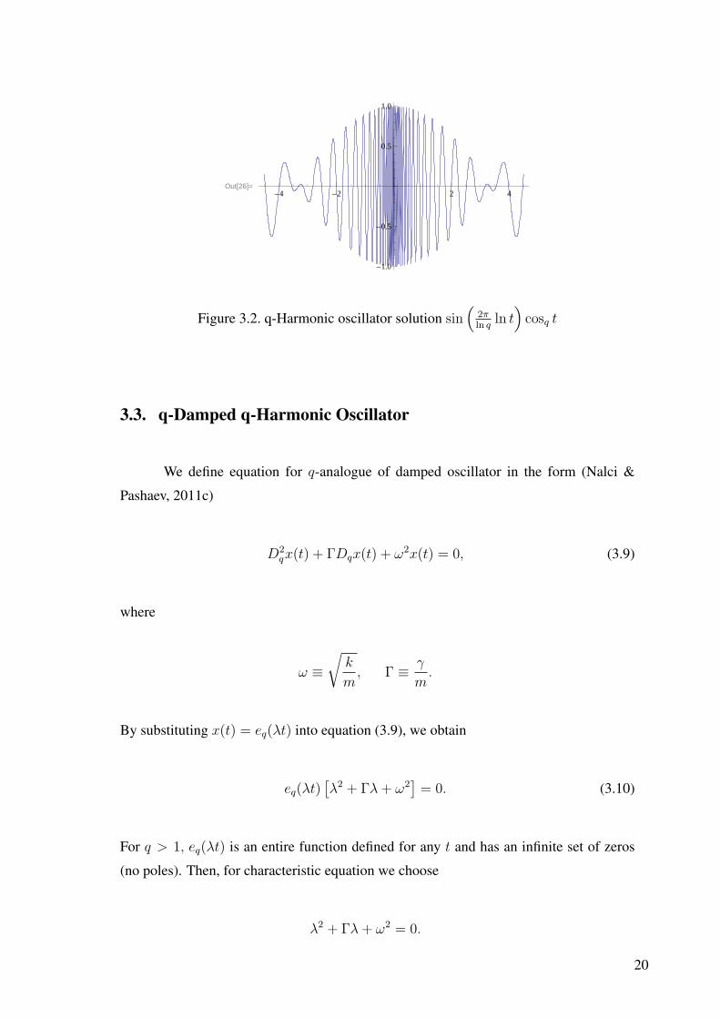
are not bounded and also have no periodicity. In Figure 3.2 we plot modulation of the

same solution with q-periodic function A(t) = sin(

2πln q

ln t)

cosq t, which gives micro

oscillations to the solution.

Out[25]= -4 -2 2 4

-1.0

-0.5

0.5

1.0

Figure 3.1. q-Harmonic oscillator solution cosq t

19

Out[26]=-4 -2 2 4

-1.0

-0.5

0.5

1.0

Figure 3.2. q-Harmonic oscillator solution sin(

2πln q

ln t)

cosq t

3.3. q-Damped q-Harmonic Oscillator

We define equation for q-analogue of damped oscillator in the form (Nalci &

Pashaev, 2011c)

D2qx(t) + ΓDqx(t) + ω2x(t) = 0, (3.9)

where

ω ≡√

k

m, Γ ≡ γ

m.

By substituting x(t) = eq(λt) into equation (3.9), we obtain

eq(λt)[λ2 + Γλ + ω2

]= 0. (3.10)

For q > 1, eq(λt) is an entire function defined for any t and has an infinite set of zeros

(no poles). Then, for characteristic equation we choose

λ2 + Γλ + ω2 = 0.

20

The roots of this characteristic equation are

λ1,2 = −Γ

2±

√Γ2

4− ω2.

3.3.1. Under-Damping Case

For Γ2 < 4ω2, we have two complex conjugate roots

λ1 = −Γ

2+ iΩ, λ2 = −Γ

2− iΩ,

where

Ω ≡√

ω2 − Γ2

4.

Then the general solution of equation (3.9) is

x(t) = Aeq

[(−Γ

2+ iΩ

)t

]+ Beq

[(−Γ

2− iΩ

)t

]. (3.11)

In Figure 3.3 and Figure 3.4 we plot particular solutions with constant (A = B = 1) and

with q-Periodic modulation, respectively.

3.3.2. Over-Damping Case

For Γ2 > 4ω2, we have two distinct real roots λ1,2 and solution is

x(t) = A(t)eq

[(−Γ

2+

√Γ2

4− ω2

)t

]+ B(t)eq

[(−Γ

2−

√Γ2

4− ω2

)t

], (3.12)

21

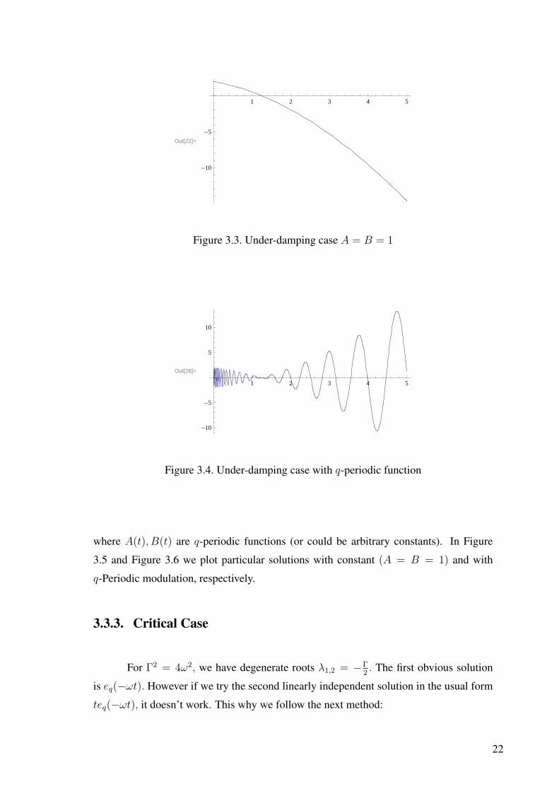
Out[22]=

1 2 3 4 5

-10

-5

Figure 3.3. Under-damping case A = B = 1

Out[28]=

1 2 3 4 5

-10

-5

5

10

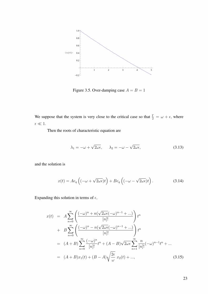
Figure 3.4. Under-damping case with q-periodic function

where A(t), B(t) are q-periodic functions (or could be arbitrary constants). In Figure

3.5 and Figure 3.6 we plot particular solutions with constant (A = B = 1) and with

q-Periodic modulation, respectively.

3.3.3. Critical Case

For Γ2 = 4ω2, we have degenerate roots λ1,2 = −Γ2. The first obvious solution

is eq(−ωt). However if we try the second linearly independent solution in the usual form

teq(−ωt), it doesn’t work. This why we follow the next method:

22

Out[45]=

1 2 3 4 5

-0.2

0.2

0.4

0.6

0.8

1.0

Figure 3.5. Over-damping case A = B = 1

We suppose that the system is very close to the critical case so that Γ2

= ω + ε, where

ε ¿ 1.

Then the roots of characteristic equation are

λ1 = −ω +√

2ωε, λ2 = −ω −√

2ωε, (3.13)

and the solution is

x(t) = Aeq

((−ω +

√2ωε)t

)+ Beq

((−ω −

√2ωε)t

). (3.14)

Expanding this solution in terms of ε,

x(t) = A

∞∑n=0

((−ω)n + n(

√2ωε(−ω)n−1 + ...)

[n]!

)tn

+ B

∞∑n=0

((−ω)n − n(

√2ωε(−ω)n−1 + ...)

[n]!

)tn

= (A + B)∞∑

n=0

(−ω)n

[n]!tn + (A−B)

√2ωε

∞∑n=1

n

[n]!(−ω)n−1tn + ...

= (A + B)x1(t) + (B − A)

√2ε

ωx2(t) + ..., (3.15)

23

Out[48]=1 2 3 4 5

-1.0

-0.5

0.5

1.0

Figure 3.6. Over-damping case with q-periodic function

in zero approximation we get the first solution

x1(t) = eq(−ωt). (3.16)

In the linear approximation we obtain the second solution in the form

x2(t) = td

dteq(−ωt). (3.17)

In Appendix A, we show that solutions x1(t) and x2(t) are linearly independent. We can

also rewrite this in terms of q-logarithm, which instead of linear in t term for q = 1 case,

now includes infinite set of arbitrary powers of t,

x2(t) =1

1− q

∞∑

l=1

((1− 1

q)ωt

)l

[l]eq(−ωt)

= − 1

1− qLnq

(1−

(1− 1

q

)ωt

)eq(−ωt). (3.18)

It is easy to check that for q → 1 our solution reduces to the standard second solution

te−ωt.

Combining the above results we find the general solution in the degenerate case

24

as

x(t) = Aeq(−ωt) + B td

dteq(−ωt). (3.19)

In Figure 3.7 and Figure 3.8 we plot particular solutions with constant (A = B = 1) and

with q-Periodic modulation, respectively.

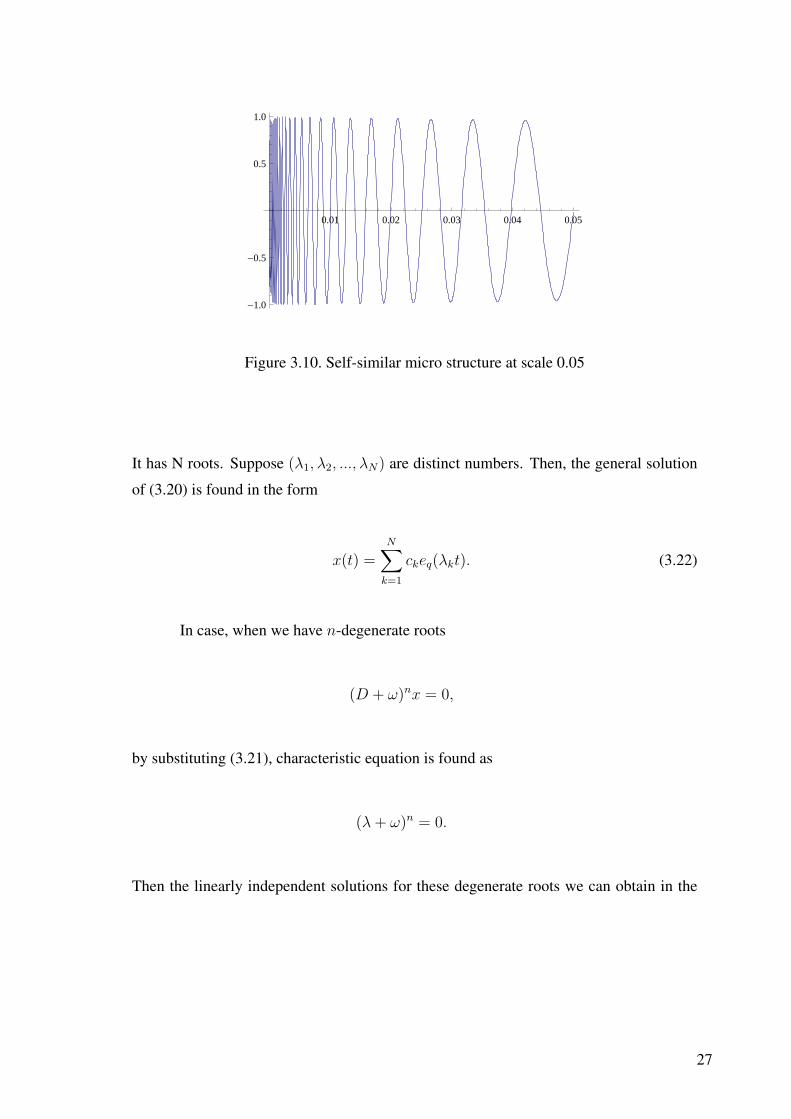
In Figures 3.9 and 3.10 we plot solution with q-Periodic function modulation at

different small scales. Comparing these figures we find very close similarity, this why

q-periodic function modulation leads to the self-similarity property of the solution.

Out[36]=

1 2 3 4 5

-1.5

-1.0

-0.5

0.5

1.0

Figure 3.7. Critical case

Out[41]=

1 2 3 4 5

-1.5

-1.0

-0.5

0.5

1.0

1.5

Figure 3.8. Critical case with periodic function

25

0.1 0.2 0.3 0.4 0.5

-1.0

-0.5

0.5

1.0

Figure 3.9. Self-similar micro structure at scale 0.5

3.4. Degenerate Roots for Equation Degree N

The result for degenerate roots obtained in previous section can be generalized

to equation of an arbitrary order (Nalci & Pashaev, 2011c). The constant coefficients

q-difference equation of order N is

N∑

k=0

akDkx(t) = 0, (3.20)

where ak are constants. By substitution

x = eq(λt) (3.21)

we get the characteristic equation

N∑

k=1

akλk = 0.

26

0.01 0.02 0.03 0.04 0.05

-1.0

-0.5

0.5

1.0

Figure 3.10. Self-similar micro structure at scale 0.05

It has N roots. Suppose (λ1, λ2, ..., λN) are distinct numbers. Then, the general solution

of (3.20) is found in the form

x(t) =N∑

k=1

ckeq(λkt). (3.22)

In case, when we have n-degenerate roots

(D + ω)nx = 0,

by substituting (3.21), characteristic equation is found as

(λ + ω)n = 0.

Then the linearly independent solutions for these degenerate roots we can obtain in the

27

following form :

x1(t) = eq(−ωt),

x2(t) = td

dteq(−ωt) =

1

q − 1Lnq

(1− (1− 1

q)ωt

)eq(−ωt),

x3(t) =

(td

dt

)2

eq(−ωt),

or by using the commutation relation[t, d

dt

]= −1, up to linearly dependent solution, it

can be written as

x3(t) = t2d2

dt2eq(−ωt),

...

xn(t) = tn−1 dn−1

dtn−1eq(−ωt).

From the following commutation relation

[td

dt, D

]= −D (3.23)

we obtain

td

dtDn = Dn

(td

dt− n

)

and

td

dt(ω + D)n = (ω + D)nt

d

dt− n(ω + D)n−1D. (3.24)

Using the operator identity (3.24) we can show that if x0 is solution of

(D + ω)x0 = 0,

then it is solution of

(D + ω)nx0 = 0.

28

Then,

x1 = td

dtx0

is solution of

(D + ω)2x1 = 0,

and as follows

(D + ω)nx1 = 0,

e.t.c. And then,

xn−1 = tdn−1

dtn−1x0

is solution of

(D + ω)nxn−1 = 0.

It provides us with n linearly independent solutions x0, x1, ..., xn−1 of N -degree equation

with n-degenerate roots

(D + ω)nx = 0.

29

CHAPTER 4

Q-SPACE-TIME DIFFERENCE HEAT EQUATION

Here we introduce q-analogue of heat equation in one space dimension (Nalci &

Pashaev, 2010)

Dtφ(x, t) = νD2xφ(x, t). (4.1)

In the limit q → 1 it reduces to the standard heat equation

φt = νφxx.

We will construct exact solutions of this equation in the form of polynomials.

4.1. q-Hermite Polynomials

We introduce the q-analogue of Hermite polynomials (Nalci & Pashaev, 2010) by

the generating function

eq(−t2)eq([2]qtx) =∞∑

n=0

Hn(x; q)tn

[n]q!. (4.2)

From the defining identity (4.2) it is not hard to derive for the q-Hermite polynomials an

explicit sum formula

Hn(x; q) =

[n/2]∑

k=0

(−1)k[n]q!

[k]q![n− 2k]q!([2]qx)n−2k. (4.3)

This explicit sum makes it transparent in which way our polynomials Hn(x; q),

q-extend the Hn(x) and how they are different from the known ones in literature. By

30

q-differentiating the generating function (4.2) with respect to x and t we derive two-term

and three-term recurrence relations correspondingly

DxHn(x; q) = [2]q[n]qHn−1(x; q), (4.4)

Hn+1(x; q) = [2]q xHn(x; q)− [n]q Hn−1(qx; q)

− [n]q qn+1

2 Hn−1(√

qx; q). (4.5)

From this generating function we have the special values

H2n(0; q) = (−1)n [2n]q!

[n]q!, (4.6)

H2n+1(0; q) = 0, (4.7)

and the parity relation

Hn(−x; q) = (−1)nHn(x; q). (4.8)

To write the three-term recurrence relation in the local form, for the same argument x, we

use dilatation operator

Mq = qx ddx , (4.9)

so that

Mqf(x) = f(qx), (4.10)

31

and relation (4.5) can be rewritten as

Hn+1(x; q) = [2]q xHn(x; q)

− [n]q(Mq + qn+1

2 M√q)Hn−1(x; q). (4.11)

Substituting (4.4) into (4.11) we get

Hn+1(x; q) =

([2]q x− Mq + q

n+12 M√

q

[2]qDx

)Hn(x; q). (4.12)

By the recursion, starting from n = 0 and H0(x) = 1 we have next representation for the

q-Hermite polynomials

Hn(x; q) =n∏

k=1

([2]q x− Mq + q

k2 M√

q

[2]qDx

)· 1. (4.13)

We notice that the generating function and the form of our q-Hermite polynomials are

different from the known ones in the literature, (Exton, 1983), (Cigler & Zeng, 2009),

(Rajkovic & Marinkovic, 2001), (Negro, 1996). Moreover, the three-term recurrence

relation (4.5) is q-nonlocal and different from the known ones for orthogonal polynomial

sets (Ismail, 2005).

In the above expression the operator

Mq + qn2 M√

q = 2qn4 q

34x d

dx cosh[(ln q14 )(x

d

dx− n)] (4.14)

is expressible in terms of the q-spherical means as

cosh[(ln q)xd

dx]f(x) =

1

2(f(qx) + f(

1

qx)). (4.15)

32

By notation for the q-shifted product, (Kac & Cheung, 2002),

(x− a)nq = (x− a)(x− qa) · · · (x− qn−1a), n = 1, 2, ..

which now we apply to the noncommutative operators, so that we should distinguish the

direction of multiplication, we have two cases

(x− a)nq < ≡ (x− a)(x− qa) · · · (x− qn−1a), (4.16)

and

(x− a)nq > ≡ (x− qn−1a) · · · (x− qa)(x− a). (4.17)

Then, we can rewrite (4.13) shortly as

Hn(x; q) =

(([2]q x− Mq Dx

[2]q)− q

12M√

q Dx

[2]q

)n

√q >

· 1.

First few polynomials are

H0(x; q) = 1,

H1(x; q) = [2]q x,

H2(x; q) = [2]2q x2 − [2]q,

H3(x; q) = [2]3q x3 − [2]2q[3]q x,

H4(x; q) = [2]4q x4 − [2]2q[3]q[4]q x2 + [2]q[3]q[2]q2 .

When q → 1 these polynomials reduce to the standard Hermite polynomials.

33

4.1.1. q-Difference Equation

Applying Dx to both sides of (4.12) and using recurrence formula (4.4) we get the

q-difference equation for the q-Hermite polynomials

1

[2]qDx(Mq + q

n+12 M√

q)DxHn(x; q)− [2]qqxDxHn(x; q) + [2]q[n]qqHn(x; q) = 0.

4.2. Operator Representation

Proposition 4.2.0.1

eq

(− 1

[2]2qD2

x

)eq([2]qxt) = eq(−t2)eq([2]qxt). (4.18)

Proof 4.2.0.2 By q- differentiating the q-exponential function with respect to x

Dnxeq([2]qxt) = ([2]t)neq([2]qxt), (4.19)

and combining then to the sum

∞∑n=0

an

[n]q!D2n

x eq([2]qxt) =∞∑

n=0

[2]2nq ant2n

[n]q!eq([2]qxt), (4.20)

we have relation

eq(aD2x)eq([2]qxt) = eq([2]2qat2)eq([2]qxt). (4.21)

By choosing a = −1/[2]2q we get the result (4.18).

34

Proposition 4.2.0.3

Hn(x; q) = [2]nq eq

(− 1

[2]2qD2

x

)xn. (4.22)

Proof 4.2.0.4 The right hand side of (4.18) is the generating function for the q-Hermite

polynomials (4.2). Hence, equating the coefficients of tn on both sides gives the result.

Proposition 4.2.0.5

eq

(−D2

x

[2]2q

)xn+1 =

1

[2]q

([2]q x− (Mq + q

n+12 M√

q)Dx

[2]q

)eq

(−D2

x

[2]2q

)xn. (4.23)

Proof 4.2.0.6 We use (4.22) and relation (4.12) .

Corollary 4.2.0.7 If function f(x) is expandable to the power series f(x) =∑∞

n=0 anxn,

then we have the next formal q-Hermite series representation

eq

(− 1

[2]2qD2

x

)f(x) =

∞∑n=0

anHn(x; q)

[2]nq. (4.24)

4.3. q- Kampe-de Feriet Polynomials

We define the q-Kampe-de Feriet polynomials as

Hn(x, νt; q) = (−νt)n2 Hn

(x

[2]q√−νt

; q

), (4.25)

so that from (4.12) we obtain the next recursion formula

Hn+1(x, νt; q) =(x + (Mq + q

n+12 M√

q)νtDx

)Hn(x, νt; q).

35

By the recursion it gives

Hn(x, νt; q) =n∏

k=1

(x + (Mq + q

k2 M√

q)νtDx

)· 1, (4.26)

or by notation (4.17)

Hn(x, νt; q) =((x + Mq νt Dx) + q

12 M√

q νtDx

)n

√q >· 1.

Then the first few polynomials are

H0(x, νt; q) = 1,

H1(x, νt; q) = x,

H2(x, νt; q) = x2 + [2]q νt

H3(x, νt; q) = x3 + [2]q[3]q νt x,

H4(x, νt; q) = x4 + [3]q[4]q νt x2 + [2]q[3]q[2]q2ν2t2.

4.4. q-Heat Equation

We introduce the q-heat equation

(Dt − νD2x)φ(x, t) = 0, (4.27)

with partial q-derivatives with respect to t and x. Solution of this equation expanded in

terms of parameter k

φ(x, t) = eq(νk2t)eq(kx) =∞∑

n=0

kn

[n]!Hn(x, νt; q), (4.28)

gives the set of q-Kampe-de Feriet polynomial solutions for the equation. Then we find

the time evolution of zeroes xk(t) for these polynomials in terms of zeroes zk(n, q) of the

36

q-Hermite polynomials,

Hn(zk(n, q), q) = 0, (4.29)

so that

xk(t) = [2]zk(n, q)√−νt. (4.30)

For n=2 we have two zeros determined by q-numbers,

x1(t) =√

[2]q√−νt, x2(t) = −

√[2]q

√−νt,

and moving in opposite directions according to (4.30). For n=3 we have zeros determined

by q-numbers,

x1(t) = −√

[3]q!√−νt, x2(t) = 0, x3(t) =

√[3]q!

√−νt,

two of which are moving in opposite direction according to (4.30) and one is in the rest.

4.5. Evolution Operator

Following similar calculations as in Proposition I we have the next relation

eq

(νtD2

x

)eq(kx) = eq(νtk2)eq(kx). (4.31)

The right hand side of this expression is the plane wave type solution (4.28) of the q-heat

equation (4.27). Equating the coefficients of kn on both sides we get the q-Kampe de

Feriet polynomial solutions of this equation

Hn(x, νt; q) = eq

(νtD2

x

)xn. (4.32)

37

Consider an arbitrary, expandable to the power series function f(x) =∑∞

n=0 anxn, then

the formal series

f(x, t) = eq

(νtD2

x

)f(x) =

∞∑n=0

aneq

(νtD2

x

)xn (4.33)

=∞∑

n=0

anHn(x, νt; q), (4.34)

represents a time dependent solution of the q-heat equation (4.27). Domain of conver-

gency for this series is determined by asymptotic properties of our q-Kampe-de Feriet

polynomials for n →∞ and requires additional study.

According to this we have the evolution operator for the q-heat equation as

U(t) = eq

(νtD2

x

). (4.35)

It allows us to solve the initial value problem

(Dt − νD2x)φ(x, t) = 0, (4.36)

φ(x, 0+) = f(x), (4.37)

in the form

φ(x, t) = eq

(νtD2

x

)φ(x, 0+) = eq

(νtD2

x

)f(x), (4.38)

where we imply the base q > 1 so that eq(x) is an entire function.

38

CHAPTER 5

Q-SPACE-TIME DIFFERENCE BURGERS’ EQUATION

5.1. Burger’s Equation and Cole-Hopf Transformation

Nonlinear Heat equation which is also known as Burger’s equation is

ut + uux = νuxx. (5.1)

By using the Cole-Hopf transformation

u(x, t) = −2νφx(x, t)

φ(x, t), (5.2)

it reduces to Linear heat equation

φt = νφxx. (5.3)

Shock soliton solutions are the particular solutions of this equation.

5.2. q-Burger’s Equation as nonlinear q-Heat Equation

We introduce the q-Cole-Hopf transformation

u(x, t) = −2νDxφ(x, t)

φ(x, t), (5.4)

39

where φ(x, t) is solution of the q-heat equation (4.27), we find that u(x, t) satisfies the

q-Burgers’ type Equation with cubic nonlinearity (Nalci & Pashaev, 2010)

Dtu(x, t)− νD2xu(x, t) =

1

2

[(u(x, qt)− u(x, t)Mx

q )Dxu(x, t)]

− 1

2[Dx (u(qx, t)u(x, t))] +

1

4ν

[u(q2x, t)− u(x, qt)

]u(qx, t)u(x, t). (5.5)

When q → 1 it reduces to the standards Burgers’ Equation

ut + uux = νuxx. (5.6)

5.2.1. I.V.P. for q-Burgers’ Type Equation

Substituting the operator solution (4.38) to (5.4), we find operator solution for the

q-Burgers type equation in the form

u(x, t) = −2νeq (νtD2

x) Dxf(x)

eq (νtD2x) f(x)

. (5.7)

This solution corresponds to the initial function

u(x, 0+) = −2νDxf(x)

f(x). (5.8)

Thus, for arbitrary initial value u(x, 0+) = F (x) for the q-Burgers equation we need to

solve the initial value problem for the q-heat equation (4.27) with initial function f(x)

satisfying the first order q-difference equation

(Dx +1

2νF (x))f(x) = 0. (5.9)

40

5.3. q-Shock Soliton

As a particular solution of the q-heat equation we choose first

φ(x, t) = eq

(k2t

)eq (kx) , (5.10)

then we find solution of the q-Burgers equation as a constant

u(x, t) = −2νk. (5.11)

We notice that for this solution of the q-heat equation, we have an infinite set of zeros, and

the space position of zeros is fixed during time evolution at points xn = −qn+1/(q− 1)k,

n = 0, 1, ....

If we choose the linear superposition

φ(x, t) = eq

(k2

1t)eq (k1x) + eq

(k2

2t)eq (k2x) , (5.12)

then we have the q-shock soliton solution

u(x, t) = −2νk1eq (k2

1t) eq (k1x) + k2eq (k22t) eq (k2x)

eq (k21t) eq (k1x) + eq (k2

2t) eq (k2x). (5.13)

This expression is the q-analogue of the Burgers shock soliton and for q → 1 it reduces

to the last one. However, in contrast to the standard Burgers case, due to zeroes of the

q-exponential function this expression admits singularities for some values of parameters

k1 and k2.

In Figure 5.1 we plot the singular q-shock soliton for k1 = 1 and k2 = 10 at time

t = 0 with base q = 10.

41

Out[2]=-4 -2 2 4

-20

-10

10

20

Figure 5.1. Singular q-shock soliton

It turns out that for some specific values of parameters we can find the regular

q-shock soliton solution. We introduce the cosine q-hyperbolic function

coshq(x) =eq(x) + eq(−x)

2, (5.14)

or

coshq(x) =1

2

(eq(x) +

1

e 1q(x)

), (5.15)

then by using the infinite product representation (2.27) for the q-exponential function we

have

coshq(x) =1

2

((1 + (1− 1

q)x

)∞

1/q

+

(1− (1− 1

q)x

)∞

q

).

From (2.28),(2.29) we find that zeroes of the first product are located on negative axis x,

while for the second product on the positive axis x. Therefore the function has no zeros

for real x and coshq(0) = 1.

If we choose k1 = 1, and k2 = −1, the time dependent factors in nominator and

42

the denominator of (5.13) cancel each other and we have the stationary shock soliton

u(x, t) = −2νeq(x)− eq(−x)

eq(x) + eq(−x)≡ −2ν tanhq(x). (5.16)

Due to the above consideration this function has no singularity on real axis and we have

regular everywhere q-shock soliton solution. In the limit q → 1 it reduces to the kink-

soliton.

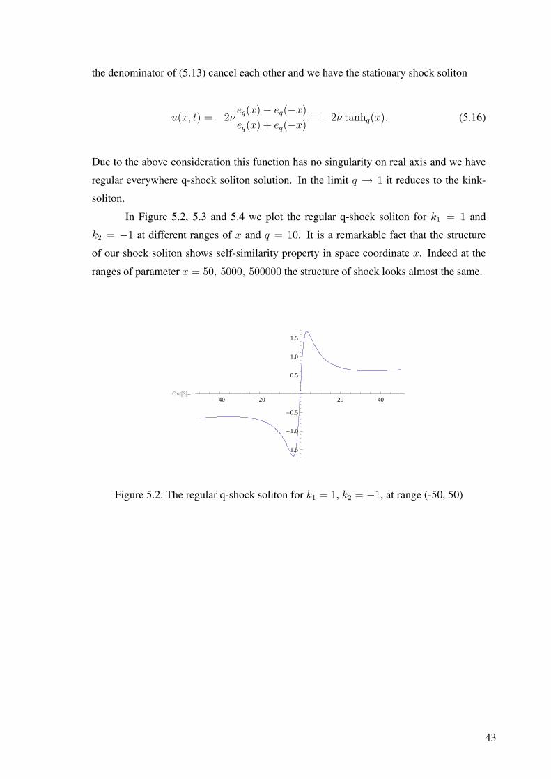
In Figure 5.2, 5.3 and 5.4 we plot the regular q-shock soliton for k1 = 1 and

k2 = −1 at different ranges of x and q = 10. It is a remarkable fact that the structure

of our shock soliton shows self-similarity property in space coordinate x. Indeed at the

ranges of parameter x = 50, 5000, 500000 the structure of shock looks almost the same.

Out[3]=-40 -20 20 40

-1.5

-1.0

-0.5

0.5

1.0

1.5

Figure 5.2. The regular q-shock soliton for k1 = 1, k2 = −1, at range (-50, 50)

43

Out[4]=-4000 -2000 2000 4000

-1.5

-1.0

-0.5

0.5

1.0

1.5

Figure 5.3. The regular q-shock soliton for k1 = 1, k2 = −1 at range (-5000, 5000)

Out[5]=-400 000 -200 000 200 000 400 000

-1.5

-1.0

-0.5

0.5

1.0

1.5

Figure 5.4. The regular q-shock soliton for k1 = 1, k2 = −1 at range (-500000, 500000)

44

Out[7]=-3 -2 -1 1 2 3

-1.0

-0.5

0.5

1.0

Figure 5.5. q-Shock soliton

Out[10]=-3 -2 -1 1 2 3

-1.5

-1.0

-0.5

0.5

1.0

1.5

Figure 5.6. q-Shock soliton with q-periodic modulation

45

Out[12]=-0.3 -0.2 -0.1 0.1 0.2 0.3

-0.4

-0.2

0.2

0.4

Figure 5.7. Self-similar q-shock soliton micro structure at scale 0.3

Out[14]=-0.03 -0.02 -0.01 0.01 0.02 0.03

-0.04

-0.02

0.02

0.04

Figure 5.8. Self-similar q-shock soliton micro structure at scale 0.03

46

For the set of arbitrary numbers k1, ..., kN

φ(x, t) =N∑

n=1

eq

(k2

nt)eq (knx) , (5.17)

we have multi-shock soliton solution in the form

u(x, t) = −2ν

∑Nn=1 kneq (k2

nt) eq (knx)∑Nn=1 eq (k2

nt) eq (knx). (5.18)

In general this solution admits several singularities. To have regular multi-shock solution

we can consider the even number of terms N = 2k with opposite wave numbers. When

N = 4 and k1 = 1, k2 = −1,k3 = 10,k4 = −10 we have q-multi-shock soliton solution,

u(x, t) = −2νeq(t) sinhq(x) + 10eq(100t) sinhq(10x)

eq(t) coshq(x) + eq(100t) coshq(10x). (5.19)

In Figure 5.9 we plot N = 4 case with values of the wave numbers k1 = 1,

k2 = −1, k3 = 10, k4 = −10 at t = 0 and q = 10. To have regular solution for any time t

and given base q, we should choose proper numbers ki which are not in the form of power

of q.

Out[4]=-40 -20 20 40

-15

-10

-5

5

10

15

Figure 5.9. Multi q-shock regular for k1 = 1, k2 = −1, k3 = 10, k4 = −10 at t = 0

47

CHAPTER 6

Q-SPACE DIFFERENCE AND TIME DIFFERENTIAL

HEAT EQUATION

6.1. q-Hermite Polynomials

We define the q-analog of Hermite polynomials by the generating function with

the Jackson’s q-exponential function and standard exponential function as (Pashaev &

Nalci, 2010)

e−t2eq([2]qtx) =∞∑

N=0

HN(x; q)tN

[N ]q!, (6.1)

where the Jackson’s q-exponential function is defined by

eq(x) =∞∑

n=0

xn

[n]q!,

[n]q! = [1]q[2]q...[n]q and q-number

[n]q =qn − 1

q − 1.

From the defining identity (6.1) it is not difficult to derive for the q-Hermite poly-

nomials an explicit sum formula

HN(x; q) =

[N/2]∑

k=0

(−1)k([2]qx)N−2k[N ]q!

k![N − 2k]q!. (6.2)

This explicit sum makes it transparent in which way our polynomials HN(x; q) q-extended

the HN(x) and how they are different from the known ones in literature. By q-differentiating

48

the generating function (6.1) with respect to x we derive two-term recurrence relation cor-

respondingly

DqHN(x; q) = [2]q[N ]qHN−1(x; q), (6.3)

where definition of q-derivative is

Dxf(x) =f(qx)− f(x)

(q − 1)x. (6.4)

By standard differentiating the generating function (6.1) with respect to t and using

the equality

td

dteq([2]qxt) = x

d

dxeq([2]qxt) =

∞∑n=0

n([2]qxt)n

[n]q!

we obtain the two-term recurrence relation

(xd

dx−N)HN(x; q) = 2[N ]q[N − 1]qHN−2(x; q). (6.5)

By standard differentiating the generating function (6.1) with respect to t and using defi-

nition of q-logarithmic function (Pashaev & Yılmaz, 2008)

Lnq(1 + z) =∞∑

N=1

(−1)N−1zN

[N ],

where q > 1, 0 < |z| < q and the property

d

dzln eq

(αz

1− q

)=

Lnq(1− αz)

(q − 1)z

49

we derive the N-term (instead of 3-term) recurrence relation formula

HN+1(x; q) =[N + 1]qN + 1

([2]qxHN(x; q)

− 2[N ]qHN−1(x; q)− (q − 1)[2]q[N ]qx2HN−1(x; q)

+ [2]q[N ]q!N−2∑

k=0

(−1)N−k(q2 − 1)N−kxN−k+1Hk(x; q)

[k]q![N − k + 1]q).

When q → 1 this multiple term recurrence relation for q-Hermite polynomials reduces to

the three-term recurrence relation for Hermite polynomials

HN+1(x) = 2xHN(x)− 2NHN−1(x).

Substituting (6.3) into N-term recurrence relation formula we get

HN+1(x; q) =

[N + 1]qN + 1

([2]qx− (

2

[2]q+ (q − 1)x2)Dx +

N∑

l=2

(−1)l(q2 − 1)lxl+1

[2]l−1q [l + 1]q

Dlx

)HN(x; q),

or

HN+1 =[N + 1]!

N + 1

(−2

HN−1

[N − 1]!+

N∑

k=0

Hk(1− q)N−k([2]x)N−k+1

[k]![N − k + 1]

)

=[N + 1]

N + 1

(−2[N ]HN−1 + [N ]!

N∑

k=0

Hk(1− q)N−k([2]x)N−k+1

[k]![N − k + 1]

). (6.6)

By the recursion, starting from n = 0 and H0(x; q) = 1 we have next representa-

tion for the q-Hermite polynomials

HN+1(x; q) =N∏

k=0

[k + 1]qk + 1

([2]qx− (

2

[2]q+ (q − 1)x2)Dx +

N∑

k=2

(−1)k(q2 − 1)kxk+1

[2]k−1q [k + 1]q

Dkx

)· 1.

50

In the limit q → 1 case this product formula is reduced to

HN(x) = (2x− d

dx)N · 1.

We note that the generating function and the form of our q-Hermite polynomials are dif-

ferent from the known ones in the literature, (Exton, 1983), (Negro, 1996), (Rajkovic &

Marinkovic, 2001), (Cigler & Zeng, 2009). Moreover, instead of three-term recurrence

relation we have multiple term recurrence relation which shows our q-Hermite polynomi-

als are different from the known ones for orthogonal polynomials sets (Ismail, 2005).

Then first few q-Hermite polynomials are

H0(x; q) = 1,

H1(x; q) = [2]q x,

H2(x; q) = [2]2q x2 − [2]q,

H3(x; q) = [2]3q x3 − [2]2q[3]q x

H4(x; q) = [2]4q x4 − [4]q[3]q[2]2q x2 +1

2[4]q!,

H5(x; q) = [2]5q x5 − [5]q[4]q[2]3q x3 +1

2[5]q![2]x. (6.7)

When q → 1 these polynomials reduce to the standard Hermite polynomials.

6.1.1. q-Difference Equation

Applying Dx to both sides of (6.3) and using recurrence formula (6.5) we get the

q-difference-differential equation for the q-Hermite polynomials

D2qHN(x; q)− [2]2q

2x

d

dxHN(x; q) +

[2]2q2

NHN(x; q) = 0. (6.8)

In q → 1 limit it reduces to the second order linear differential equation for Her-

51

mite polynomials

d2

dx2HN(x)− 2x

d

dxHN(x) + 2NHN(x) = 0.

6.2. q-Kampe-de Feriet Polynomials

We define the q-Kampe-de Feriet polynomials as

HN(x, νt; q) = (−νt)N2 HN

(x

[2]q√−νt

; q

), (6.9)

so that from N-term recurrence relation for q-Hermite polynomial we obtain N-term re-

currence relation formula for q-Kampe-de Feriet polynomials

HN+1(x, νt; q) = [N+1]qN+1

[xHN(x, νt; q) + 2νt[N ]qHN−1(x, νt; q)

− 1[2]q

(q − 1)[N ]qx2HN−1(x, νt; q) + [N ]q!

∑N−2k=0

(−1)N−k(q2−1)N−kxN−k+1Hk(x,νt;q)

[k]q ![N−k+1]q [2]N−kq

]

or

HN+1(x, ν; q) =[N + 1]

N + 1

(2νt[N ]HN−1 +

N∑

k=0

(1− q)N−kxN−k+1Hk

[k]![N − k + 1]

).

This can also be written in terms of Dx operator form correspondingly

HN+1(x, νt; q) =

[N + 1]qN + 1

[x + (2νt +

1− q

[2]qx2)Dx +

N∑

l=2

(−1)l(q2 − 1)lxl+1

[2]lq[l]qDl

x

]HN(x, νt; q).

52

By the recursion, starting from n = 0 and H0(x, νt; q) = 1 we have next representation

for the q-Kampe-de Feriet polynomials

HN+1(x, νt; q) =N∏

k=0

[k + 1]qk + 1

[x + (2νt +

1− q

[2]qx2)Dx +

N∑

k=2

(−1)k(q2 − 1)kxk+1

[2]kq [k]qDk

x

]· 1.

In q → 1 case we have

HN(x) = (x + 2νtd

dx)N · 1.

Then the first few q-Kampe-de Feriet polynomials are

H0(x, νt; q) = 1,

H1(x, νt; q) = x,

H2(x, νt; q) = x2 + [2]q νt,

H3(x, νt; q) = x3 + [2]q[3]q νt x,

H4(x, νt; q) = x4 + [3]q[4]q νt x2 +[4]q!

2ν2t2,

H5(x, νt; q) = x5 + [4]q[5]q νt x3 +[5]q!

2ν2t2x.

When q → 1 these polynomials reduce to the standard Kampe-de Feriet polynomials.

6.3. q-Heat Equation

We introduce the q-Heat equation

(∂t − νD2x)φ(x, t) = 0 (6.10)

53

with partial q-derivative with respect to x and with partial standard derivative in time t.

One can easily see that

φk(x, t) = eνk2teq(kx)

is a plane wave solution of (6.10). By expanding this in terms of parameter k

φk(x, t) = eνk2teq(kx) =∞∑

N=0

HN(x, νt; q)kN

[N ]q!(6.11)

we get the set of q-Kampe-de Feriet polynomial solutions for the q-Heat equation (6.10).

From the defining identity (6.11) is not difficult to derive an explicit sum formula for the

q-Kampe de Feriet polynomials

HN(x, νt; q) =

[N/2]∑

k=0

(νt)kxN−2k[N ]q!

k![N − 2k]q!. (6.12)

6.3.1. Operator Representation

Proposition 6.3.1.1

e− 1

[2]2qD2

xeq([2]qxt) = e−t2eq([2]qxt). (6.13)

Proof 6.3.1.2 By q- differentiating the q-exponential function with respect to x

Dnxeq([2]qxt) = ([2]t)neq([2]qxt), (6.14)

and combining then to the sum

∞∑n=0

an

n!D2n

x eq([2]qxt) =∞∑

n=0

([2]qt)2nan

n!eq([2]qxt), (6.15)

54

we have relation

eaD2x eq([2]qxt) = ea([2]qt)2 eq([2]qxt). (6.16)

By choosing a = −1/[2]2q we get the result (10.31).

Proposition 6.3.1.3

HN(x; q) = [2]Nq e− 1

[2]2qD2

xxN . (6.17)

Proof 6.3.1.4 The right hand side of (10.31) is the generating function for the q-Hermite

polynomials (6.1). Hence, equating the coefficients of tn on both sides gives the result.

Corollary 6.3.1.5 If function f(x) is expandable to the formal power series f(x) =∑∞

N=0 aNxN then we have next q-Hermite series

e− 1

[2]2qD2

xf(x) =

∞∑N=0

aNHN(x; q)

[2]Nq. (6.18)

6.4. Evolution Operator

Following similar calculations as in Proposition I we have the next relation

eνtD2xeq(kx) = eνtk2

eq(kx). (6.19)

The right hand side of this expression is the plane wave type solution of the q-heat equa-

tion (6.10). Expanding both sides in power series in k and equating the coefficients of kN

on both sides we get q-Kampe de Feriet polynomial solutions of this equation

HN(x, νt; q) = eνtD2xxN . (6.20)

55

Consider an arbitrary, expandable to the power series function f(x) =∑∞

n=0 anxn,

then the formal series

f(x, t) = eνtD2xf(x) =

∞∑n=0

aneνtD2xxn (6.21)

=∞∑

n=0

anHN(x, νt; q), (6.22)

represents a time dependent solution of the q-heat equation (6.10). The domain of con-

vergency for this series is determined by asymptotic properties of our q-Kampe-de Feriet

polynomials for n →∞ and requires additional study.

According to this we have the evolution operator for the q-heat equation as

U(t) = eνtD2x . (6.23)

It allows us to solve the initial value problem

(∂

∂t− νD2

x)φ(x, t) = 0, (6.24)

φ(x, 0+) = f(x), (6.25)

in the form

φ(x, t) = eνtD2xφ(x, 0+) = eνtD2

xf(x), (6.26)

where we imply the base q > 1 so that eq(x) is an entire function.

56

CHAPTER 7

Q-SPACE DIFFERENCE AND TIME DIFFERENTIAL

BURGER’S EQUATION

7.1. q-Cole-Hopf Transfomation and q-Burger’s Equation

We use the q-Cole-Hopf transformation (Nalci & Pashaev, 2010)

u(x, t) = −2νDxφ(x, t)

φ(x, t), (7.1)

where φ(x, t) is solution of the q-heat equation (6.10). Then u(x, t) satisfies the q-

Burgers’ type Equation with cubic nonlinearity

∂∂t

u(x, t)− νD2xu(x, t) = 1

2

[(1−Mx

q )u(x, t)Dxu(x, t)]−

12[Dx (u(qx, t)u(x, t))] + 1

4ν[u(q2x, t)− u(x, qt)] u(qx, t)u(x, t).

When q → 1 it reduces to the standards Burgers’ Equation

ut + uux = νuxx. (7.2)

7.1.1. I.V.P. for q-Burgers’ Type Equation

Substituting the operator solution (6.26) to (7.1) we find operator solution for the

q-Burgers type equation in the form

u(x, t) = −2νeνtD2

xDxf(x)

eνtD2xf(x)

. (7.3)

57

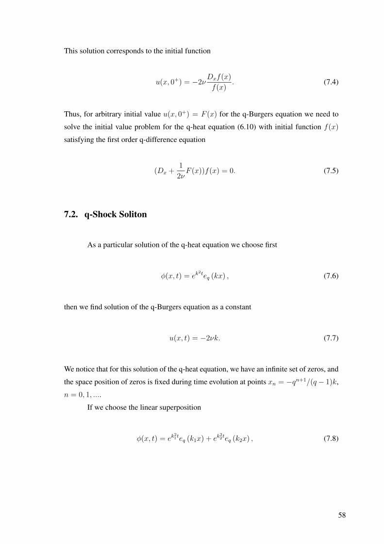
This solution corresponds to the initial function

u(x, 0+) = −2νDxf(x)

f(x). (7.4)

Thus, for arbitrary initial value u(x, 0+) = F (x) for the q-Burgers equation we need to

solve the initial value problem for the q-heat equation (6.10) with initial function f(x)

satisfying the first order q-difference equation

(Dx +1

2νF (x))f(x) = 0. (7.5)

7.2. q-Shock Soliton

As a particular solution of the q-heat equation we choose first

φ(x, t) = ek2teq (kx) , (7.6)

then we find solution of the q-Burgers equation as a constant

u(x, t) = −2νk. (7.7)

We notice that for this solution of the q-heat equation, we have an infinite set of zeros, and

the space position of zeros is fixed during time evolution at points xn = −qn+1/(q− 1)k,

n = 0, 1, ....

If we choose the linear superposition

φ(x, t) = ek21teq (k1x) + ek2

2teq (k2x) , (7.8)

58

then we have the q-Shock soliton solution

u(x, t) = −2νk1e

k21teq (k1x) + k2e

k22teq (k2x)

ek21teq (k1x) + ek2

2teq (k2x). (7.9)

This expression is the q-analog of the Burgers shock soliton and for q → 1 it reduces to

the last one. However, in contrast to the standard Burgers case, due to zeroes of the q-

exponential function this expression admits singularities coming from x for some values

of parameters k1 and k2. To have regular solution we can follow similar approach from

(Nalci & Pashaev, 2010) for k2 = −k1 we have the stationary shock soliton

u(x, t) = −2νk1eq(k1x)− eq(−k1x)

eq(k1x) + eq(−k1x)≡ −2νk1 tanhq(k1x). (7.10)

This function has no singularity on the real axis and everywhere we have regular q-shock

soliton. If we plot the regular q-shock soliton evolution for k1 = 1 and k2 = −1 at

different ranges of x and with q = 10, it is remarkable fact that the structure of our q-

shock soliton shows self-similar property in the space coordinate x. Indeed at the range

of parameter −50 < x < 50,and −5000 < x < 5000, structure of shock looks almost the

same (Figures 5.2, 5.3 and 5.4).

However time evolution of shock solitons in (Nalci & Pashaev, 2010) produce

singularity at finite time. Here we like to find regular in x shock soliton which is regular

at any time.

We can choose solution of q-Heat equation (6.10) as

φ(x, t) = 10 + ek21teq (k1x) + ek2

2teq (k2x) ,

then for k1 = 1 and k2 = −1 we get the q-shock soliton

u(x, t) = −2νeq(x)− eq(−x)

10e−t + eq(x) + eq(−x).

This solution describes evolution of shock soliton, so that at t → −∞, u(x, t) → 0, and

for t → ∞, u(x, t) → −2ν tanhq x. In Figures 7.1, 7.2 and 7.3 we plot the regular q-

shock soliton for k1 = 1 and k2 = −1 at different time t = −2, 0, 5 with base q = 10. In

59

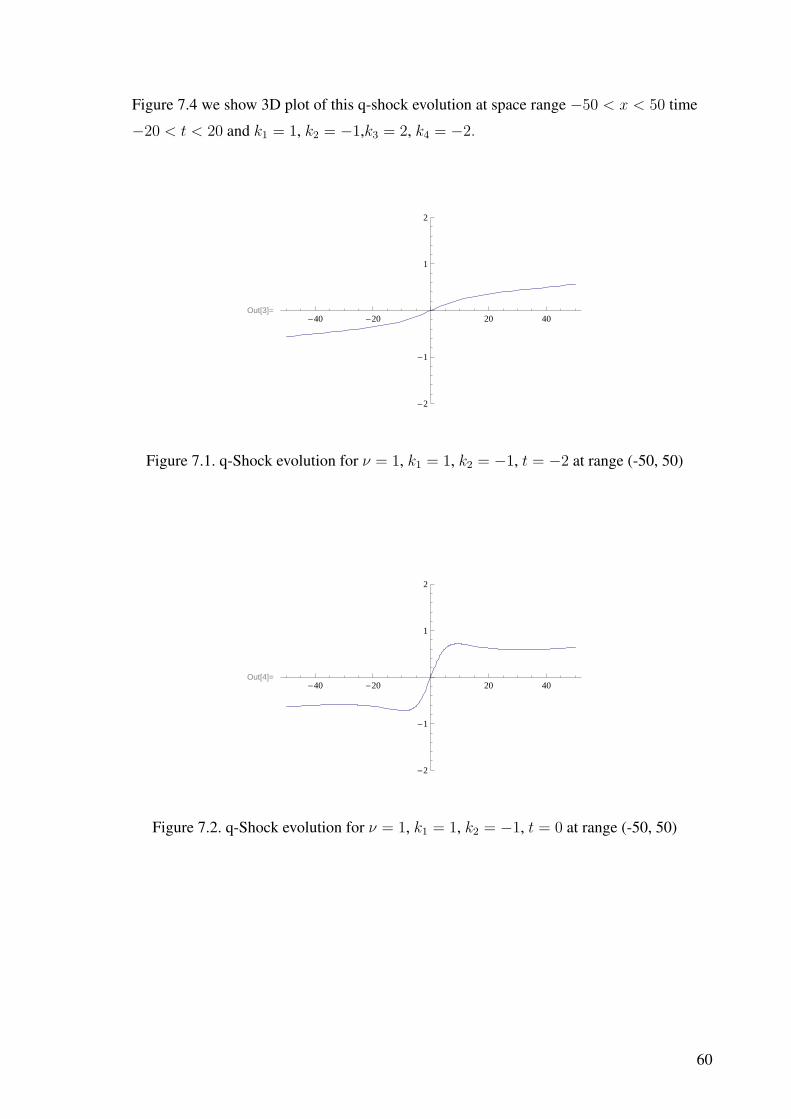
Figure 7.4 we show 3D plot of this q-shock evolution at space range −50 < x < 50 time

−20 < t < 20 and k1 = 1, k2 = −1,k3 = 2, k4 = −2.

Out[3]=-40 -20 20 40

-2

-1

1

2

Figure 7.1. q-Shock evolution for ν = 1, k1 = 1, k2 = −1, t = −2 at range (-50, 50)

Out[4]=-40 -20 20 40

-2

-1

1

2

Figure 7.2. q-Shock evolution for ν = 1, k1 = 1, k2 = −1, t = 0 at range (-50, 50)

60

Out[6]=-40 -20 20 40

-2

-1

1

2

Figure 7.3. q-Shock evolution for ν = 1, k1 = 1, k2 = −1, t = 5 at range (-50, 50)

For the set of arbitrary numbers k1, ..., kN

φ(x, t) =N∑

n=1

ek2nteq (knx) , (7.11)

we have multi-shock solution in the form

u(x, t) = −2ν

∑Nn=1 kne

k2nteq (knx)∑N

n=1 ek2nteq (knx)

. (7.12)

In general this solution admits several singularities. To have a regular multi-shock

solution we can consider the even number of terms N = 2k with opposite wave numbers.

When N = 4 and k1 = 1, k2 = −1,k3 = 2,k4 = −2 we have q-multi-shock soliton

solution,

u(x, t) = −2νsinhq(x) + 2e3t sinhq(2x)

coshq(x) + e3t coshq(2x). (7.13)

61

Out[8]=

-50

0

50

-20

-10

0

10

20

-1

0

1

Figure 7.4. 3D plot of q-shock evolution for k1 = 1, k2 = −1,k3 = 2, k4 = −2 and atrange (-50, 50)

In Figures 7.5, 7.6 and 7.7 we plot N = 4 case with values of the wave numbers

k1 = 1, k2 = −1, k3 = 2, k4 = −2 at t = −10, 0, 7 and with q = 10. In Figure 7.8 we

show 3D plot of of this multiple q-shock evolution. This multi-shock soliton is regular

everywhere in x for arbitrary time t. This result takes place due to absence of zeros for

the standard exponential function ek2t.

62

Out[21]=-40 -20 20 40

-4

-2

2

4

Figure 7.5. Multi q-shock evolution for k1 = 1, k2 = −1,k3 = 2, k4 = −2, t = −10and at range (-50, 50)

Out[39]=-40 -20 20 40

-4

-2

2

4

Figure 7.6. Multi q-shock evolution for k1 = 1, k2 = −1,k3 = 2, k4 = −2, t = 0 andat range (-50, 50)

63

Out[31]=-40 -20 20 40

-4

-2

2

4

Figure 7.7. Multi q-shock evolution for k1 = 1, k2 = −1,k3 = 2, k4 = −2, t = 7 andat range (-50, 50)

Out[41]=

-50

0

50

-10

-5

0

5

-4

-2

0

2

4

Figure 7.8. 3D plot of multiple q-shock evolution for k1 = 1, k2 = −1,k3 = 2, k4 =−2, and at range (-50, 50)

64

CHAPTER 8

Q-SCHRODINGER EQUATION AND Q-MADDELUNG

FLUID

8.1. Standard Time-Dependent q-Schrodinger Equation

The above consideration can be extended to the time dependent Schodinger equa-

tion with q-deformed dispersion. We consider the standard time-dependent q-Schodinger

equation

(∂

∂t− i~

2mD2

x

)ψ(x, t) = 0, (8.1)

where ψ(x, t) is complex wave function (Pashaev & Nalci, 2010).

One can easily see that

ψ(x, t) = e−i~

p2

2mteq

(i

~px

)

is the plane wave solution of (8.1). By expanding this in terms of momentum p

ψ(x, t) = e−i~

p2

2mteq

(i

~px

)=

∞∑N=0

(i

~)N pN

[N ]q!H

(s)N (x, it; q)

we get the set of complex q-Kampe-de Feriet polynomial solutions

H(s)N (x, it; q) =

[N/2]∑

k=0

( iht2m

)k[N ]q!xN−2k

[N − 2k]qk!

for (8.1).

65

Let us consider the complex q-Cole-Hopf transformation

u(x, t) = −i~m

Dxψ(x, t)

ψ(x, t),

then complex velocity function u(x, t) satisfies the complex q-Burgers Madelung equation

i~ ∂∂t

u(x, t) + ~22m

D2xu(x, t) = i~

2u(x, t)[1−Mx

q ]Dxu(x, t)−

ih2

[Dx (u(qx, t)u(x, t))] + m2

[u(q2x, t)− u(x, t)] u(qx, t)u(x, t).

If we write u = u1 + iu2 and separate it into real and complex parts , we get two fluid

model representation.

For the real part we have

−~ ∂∂t

u2(x, t) + ~22m

D2xu1(x, t) = m

2[(u1(q

2x, t)− u1(x, t))(u1(x, t)u1(qx, t)−

u2(x, t)u2(qx, t))− (u2(q2x, t)− u2(x, t))(u1(x, t)u2(qx, t) + u2(x, t)u1(qx, t))]

−~2[u1(x, t)[1−Mx

q ]Dxu2(x, t) + u2(x, t)[1−Mxq ]Dxu1(x, t)]

+~2Dx[u2(qx, t)u1(x, t) + u1(qx, t)u2(x, t)],

and for imaginary part

~ ∂∂t

u1(x, t) + ~22m

D2xu2(x, t) = m

2[(u1(q

2x, t)− u1(x, t))

(u1(x, t)u2(qx, t) + u2(x, t)u1(qx, t))+

(u2(q2x, t)− u2(x, t))(u1(x, t)u1(qx, t)− u2(x, t)u2(qx, t))]+

~2[u1(x, t)[1−Mx

q ]Dxu1(x, t)− u2(x, t)[1−Mxq ]Dxu2(x, t)]−

~2Dx[u1(qx, t)u1(x, t)− u2(qx, t)u2(x, t)].

66

When q → 1, the real part reduces to the Continuity equation

−(u2)t +~

2m(u1)xx = (u1u2)x,

and imaginary part reduces to the Quantum Hamilton-Jacobi equation

(u1)t +~

2m(u2)xx = −1

2(u2

1 − u22)x.

For u1 ≡ v and u2 = − ~2m

(ln ρ)x where ρ = |ψ|2 the continuity equation is

ρt + (ρv)x = 0,

and the Euler equation is

vt + vvx =

(~2

2m2

(√

ρ)xx√ρ

)

x

.

67

CHAPTER 9

MULTIPLE Q-CALCULUS

In previous chapters we deal with q- calculus with one base q. In general, if we

consider function of several variables, every independent variable can be re-scaled by

different base parameters q1, q2, .... This why even from this general consideration, emer-

gency of multiple q-calculus becomes evident. Moreover, several physical and mathemat-

ical problems lead to necessity of multiple q-calculus. We will mention some of them.

Extension of quantum groups to two parameters (Chakrabarti & Jagannathan, 1991),

formulation of hierarchy of integrable systems in terms of recursion operator (Pashaev,

2009), discover of Q-commutative q-binomial expansion (Nalci & Pashaev, 2011d).

9.1. Multiple q- Numbers

Let us consider basis vector −→q with coordinates q1, q2, ..., qN so that the matrix

q-number can be defined as

[n]qi,qj≡ qn

i − qnj

qi − qj

= [n]qj ,qi, (9.1)

which is symmetric. Hence, we can define N ×N matrix with q-numbers elements in the

following form

([n]qi,qj

)=

[n]q1,q1 [n]q1,q2 ... [n]q1,qN

[n]q2,q1[n]q2,q2 ... [n]q2,qN

... ... ... ...

[n]qN ,q1[n]qN ,q2 ... [n]qN ,qN

. (9.2)

Diagonal terms of this matrix are defined in the limit qj → qi as

limqj→qi

[n]qi,qj= lim

qj→qi

qni − qn

j

qi − qj

= nqn−1i .

68

So this symmetric matrix can be also written as

([n]qi,qj

)=

nqn−11 [n]q1,q2 ... [n]q1,qN

[n]q1,q2nqn−1

2 ... [n]q2,qN

... ... ... ...

[n]q1,qN[n]q2,qN ... nqn−1

N

. (9.3)

As for standard numbers we may determine addition formula for q-numbers in the form

[n + m]qi,qj= qn

i [m]qi,qj+ qm

j [n]qi,qj. (9.4)

The substraction formula can be obtained by changing m → −m as

[n−m]qi,qj= qn

i [−m]qi,qj+ q−m

j [n]qi,qj, (9.5)

or by using the equality

[−n]qi,qj= −(qiqj)

−n[n]qi,qj,

it can be also written

[n−m]qi,qj= q−m

j ([n]qi,qj− qn−m

i [m]qi,qj).

We can easily prove by definition, the multiplication rule are given by next formula

[nm]qi,qj= [n]qi,qj

[m](qiqj)n = [m]qi,qj[n](qiqj)m ,

where (qiqj)m = qm

i · qmj in the standard product, and the division rule is

[ n

m

]qi,qj

=[n]qi,qj

[m]q

nmi ,q

nmj

=

[n]q

1mi ,q

1mj

[m]q

1mi ,q

1mj

. (9.6)

69

9.1.1. Multiple q-Derivative

In our multi-variable q-calculus we define q-derivative with base qi, qj as

Dqi,qjf(x) =

f(qix)− f(qjx)

(qi − qj)x. (9.7)

It represents N × N matrix of q-derivative operators D = (Dqi,qj) which is symmetric :

Dqi,qj= Dqj ,qi

where i, j = 1, 2, ..., N .

D = (Dqi,qj ) =

Dq1,q1 Dq1,q2 ... Dq1,qN

Dq2,q1 Dq2,q2 ... Dq2,qN

... ... ... ...

DqN ,q1 DqN ,q2 ... DqN ,qN

. (9.8)

If f(x) is analytic function, q-multiple derivative operator is written as follows

Dqi,qj=

Mqi−Mqj

(qi − qj)x=

qx d

dxi − q

x ddx

j

(qi − qj)x=

1

x[x

d

dx]qi,qj

.

To determine diagonal terms of this matrix D-operator (Dqi,qi)

where i = 1, 2, ..., N, we consider its action on analytic function f(x) in the form

f(x) =∞∑

n=0

anxn

so that

limqj→qi

Dqi,qjf(x) =

∞∑n=1

an limqj→qi

qni − qn

j

qi − qj

xn−1

=∞∑

n=1

ann(qix)n−1 = f ′(qix) = Mqi

d

dxf(x),

where Mqf(x) = f(qx) = qx ddx f(x). Therefore, the matrix of D-operator can be rewrit-

ten in the following form

70

D = (Dqi,qj ) =

qx d

dx1

ddx Dq1,q2 ... Dq1,qN

Dq1,q2 qx d

dx2

ddx ... Dq2,qN

... ... ... ...

Dq1,qN Dq2,qN ... qx d

dxN

ddx

. (9.9)

Example of application the q-multiple derivative of function xn is calculated by using the

(9.7) as follows

Dqi,qjxn =

(qix)n − (qjx)n

(qi − qj)x=

qni − qn

j

qi − qj

xn−1 = [n]qi,qjxn−1.

9.1.2. N = 1 Case

For N = 1 case, q1 = q2 ≡ q we have [n]q,q = nqn−1 and Dq,q = Mqddx

where

Mq = qx ddx . If in addition q = 1, then we get the standard number [n]1,1 = n and

derivative D1,1 = ddx

.

9.1.3. N = 2 Cases

For N = 2 case, we have

[n]q1,q1 = nqn−11 , [n]q1,q2 = [n]q2,q1 =

qn1 − qn

2

q1 − q2

, [n]q2,q2 = nqn−12

Dq1,q1 = Mq1

d

dx, Dq1,q2 = Dq2,q1 =

Mq1 −Mq2

(q1 − q2)x, Dq2,q2 = Mq2

d

dx.

71

9.1.3.1. Non-symmetrical Case

Choosing q1 = 1 and q2 = q we obtain,

[n]1,1 = n, [n]1,q = [n]q,1 = [n]q, [n]q,q = nqn−1.

D1,1 =d

dx, D1,q = Dq,1 =

1−Mq

(1− q)x= Dx

q , Dq,q = Mqd

dx.

In this case, for (1,1)-elements we have standard number and derivative. For non-diagonal

element we have q-number [n]q = qn−1q−1

, and q-derivative Dxq f(x) = f(qx)−f(x)

(q−1)xwhich

corresponds to non-symmetrical q-calculus with base q.

9.1.3.2. Symmetrical Case

When we choose q1 = q and q2 = 1q, we get

[n]q,q = nqn−1, [n]q, 1q

= [n]q, [n] 1q, 1q

= n

(1

q

)n−1

.

Dq,q = Mqd

dx, Dq, 1

q= D 1

q,q =

Mq −M 1q

(q − 1q)x

= Dxq , D 1

q, 1q

= M 1q

d

dx.

In this particular case we obtain symmetrical q-calculus with symmetrical q-number with

[n]q = qn−q−n

q−q−1 and symmetrical q-derivative Dxq f(x) = f(qx)−f(q−1x)

(q−q−1)x.

We can give geometrical meaning for choosing this reduction of (qi, qj)- generic

case to the symmetrical one. If we consider unit circle in complex plane, then two real

points qi = q and qj = 1q

are symmetrical points according to the unit circle. So in sym-

metrical calculus we are comparing value of function at two symmetrical points. If we

extend this reduction to the complex domain so that q is complex number, then symmet-

rical point in the unit circle would be 1q. It implies complexification of symmetrical case

in the form qi = q, qj = 1q.

72

9.1.3.3. Fibonacci Case

By choosing q1 = 1+√

52

≡ ϕ and q2 = 1−√52

≡ − 1ϕ

which are the roots of equation

(Koshy, 2001)

ϕ2 = ϕ + 1

we have q- Binet-Fibonacci numbers with bases ϕ and − 1ϕ

in the following form

[n]ϕ,ϕ = nϕn−1, [n]ϕ,− 1ϕ

= Fn, [n]− 1ϕ

,− 1ϕ

= n

(− 1

ϕ

)n−1

.

Dϕ,ϕ = Mϕd

dx, Dϕ,− 1

ϕ= D− 1

ϕ,ϕ =

Mϕ −M− 1ϕ

(ϕ + 1ϕ)x

, D− 1ϕ

,− 1ϕ

= M− 1ϕ

d

dx.

From this particular choices of basis, we obtain the Fibonacci sequence in Binet’s repre-

sentation as a q-number (Pashaev & Nalci, 2011a)

[n]ϕ,− 1ϕ

=ϕn − (− 1

ϕ)n

ϕ + 1ϕ

= Fn

and Golden derivative (ϕ-derivative)

Dxϕf(x) =

f(ϕx)− f(−ϕ−1x)

(ϕ + ϕ−1)x.

Geometrical meaning for Fibonacci case is that point ϕ on real axis outside of

unit circle (ϕ > 1) determines the symmetrical point 1ϕ

inside of circle, and the inverse

symmetrical point ϕ′ = − 1ϕ. This why, in Fibonacci case we compare function at point ϕ

and inverse symmetrical point − 1ϕ.

9.1.3.4. Symmetrical Golden Case

The Golden ratio ϕ satisfies algebraic relation

ϕ2 = ϕ + 1.

73

If we like to construct symmetrical calculus with base q as a Golden Ratio ϕ : q = ϕ,

then we choose qi = ϕ, qj = 1ϕ,

[n]ϕ, 1ϕ

= ϕn − 1

ϕn.

Another option is pure imaginary Golden ratio qi = iϕ and symmetrical point qj = iϕ

:

[n]iϕ, iϕ

= in−1[n]ϕ.

9.1.4. q-Leibnitz Rule

We derive the q-analogue of Leibnitz formula

Dqi,qj(f(x)g(x)) = Dqi,qj

f(x)g(qix) + f(qjx)Dqi,qjg(x). (9.10)

By symmetry, we can interchange i ↔ j and the second form of the Leibnitz rule can be

derived as

Dqj ,qi(f(x)g(x)) = Dqi,qj

f(x)g(qjx) + f(qix)Dqi,qjg(x), (9.11)

which is equivalent to (9.10). These formulas can be rewritten in explicitly symmetrical

form :

Dqi,qj(f(x)g(x)) = Dqi,qj

f(x)

(g(qix) + g(qjx)

2

)

+ Dqi,qjg(x)

(f(qix) + f(qjx)

2

). (9.12)

74

More general form of the q-analogue of Leibnitz formula is given with arbitrary α ,

Dqi,qj(f(x)g(x)) = (αf(qjx) + (1− α)f(qix)) Dqi,qj

g(x)

+ (αg(qix) + (1− α)g(qjx)) Dqi,qjf(x).

If we choose α = 1, we have (9.10) and (9.11), and for α = 12, (9.12) is obtained.

Now we may compute the q-multiple derivative of the quotient of f(x) and g(x).

From (9.10) we have

Dqi,qj

(f(x)

g(x)

)=

Dqi,qjf(x)g(qix)−Dqi,qj

g(x)f(qix)

g(qix)g(qjx). (9.13)

However, if we use (9.11), we get

Dqi,qj

(f(x)

g(x)

)=

Dqi,qjf(x)g(qjx)−Dqi,qj

g(x)f(qjx)

g(qix)g(qjx). (9.14)

In addition to the formulas (9.13) and (9.14) one may determine one more repre-

sentation in symmetrical form

Dqi,qj

(f(x)

g(x)

)=

1

2

Dqi,qjf(x)(g(qjx) + g(qix))−Dqi,qj

g(x)(f(qjx) + f(qix))

g(qix)g(qjx)(9.15)

In particular application one of these forms could be more useful than others.

9.1.5. Generalized Taylor Formula

In developing q-analogue of the Taylor expansion the next theorem play the central

role (Kac & Cheung, 2002):

Theorem 9.1.5.1 Let a be a number, D be a linear operator on the space of polynomials,

and P0(x), P1(x), P2(x), ... be a sequence of polynomials satisfying three conditions :

(i) P0(a) = 1 and Pn(a) = 0 for any n ≥ 1 ;

(ii) deg Pn = n ;

75

(iii) DPn(x) = Pn−1(x) for any n ≥ 1 , and D(1) = 0 Then, for any polynomial f(x) of

degree N, one has the following generalized Taylor formula :

f(x) =N∑

n=0

(Dnf)(a)Pn(x).

Here we will construct the sequence of polynomials P0(x), P1(x), P2(x), ... sat-

isfying the three above mentioned conditions of the theorem with respect to operator

D ≡ Dqi,qj.

a) First we consider the case a = 0. Then we can choose

Pn(x) =xn

[n]qi,qj!,

where [n]qi,qj! = [1]qi,qj

[2]qi,qj...[n]qi,qj

; since as easy to see

(i) P0(0) = 1, Pn(0) = 0 for n ≥ 1,

(ii) degPn = n,

(iii) for n ≥ 1,

Dqi,qjPn(x) =

Dqi,qjxn

[n]qi,qj!

=[n]qi,qj

xn−1

[n]qi,qj!

=xn−1

[n− 1]qi,qj!= Pn−1(x).

b) In more general case, when a 6= 0, to find proper polynomials Pn(x) is not

simple task. To do this we construct the first few Pn(x) and then deduce a general form

for Pn(x). We have

P0(x) = 1.

In order that Dqi,qjP1(x) = 1 and P1(a) = 0, we choose

P1(x) = x− a.

76

For the next polynomial, Dqi,qjP2(x) = x− a and P2(a) = 0, we have

P2(x) =(x− qia)(x− qja)

[2]qi,qj!

.

Similarly,

P3(x) =(x− q2

i a)(x− qiqja)(x− q2j a)

[3]qi,qj!

,

and

P4(x) =(x− q3

i a)(x− q2i qja)(x− qiq

2j a)(x− q3

j a)

[4]qi,qj!

.

Then we guess

Pn(x) =(x− a

(n)1 a)(x− a

(n)2 a)...(x− a

(n)n a)

[n]qi,qj!

, (9.16)

where

a(n)k = qn−k

i qk−1j ,

and

Pn(x) =1

[n]qi,qj!(x− qn−1

i a)(x− qn−2i qja)...(x− qiq

n−2j a)(x− qn−1

j a). (9.17)

This polynomial can also be written in the following form

Pn(x) =(x− qn−1

i a)(x− qn−1i Qa)(x− qn−1

i Q2a)...(x− qn−1i Qn−1a)

[n]qi,qj!

=(x− qn−1

i a)nQ

[n]qi,qj!

, (9.18)

where Q ≡ qj

qi.

77

If we denote qn−1i a ≡ b

(n−1)i ,then (9.18) may be written as

Pn(x) =(x− b

(n−1)i )(x−Qb

(n−1)i )(x−Q2b

(n−1)i )...(x−Qn−1b

(n−1)i )

[n]qi,qj!

,

where n = 1, 2, ... We can prove that these Pn(x) polynomials satisfy the condition (iii)

for the above Theorem. Below we follow the next definition:

Definition 9.1.5.2 The multiple q-analogue of (x− a)n is the polynomial

(x− a)nqi,qj

=

1 if n = 0,

(x− qn−1i a)(x− qn−2

i qja)...(x− qiqn−2j a)(x− qn−1

j a) if n ≥ 1

These polynomials have several properties. Factorization of symmetrical multiple q-

binomial formula is

(x− a)n+mqi,qj

= (x− qmi a)n

qi,qj(x− qn

j a)mqi,qj

= (x− qmj a)n

qi,qj(x− qn

i a)mqi,qj

.

Substituting m by −n, we can write

(x− a)n−nqi,qj

= (x− q−ni a)n

qi,qj(x− qn

j a)−nqi,qj

,

and it gives

(x− qnj a)−n

qi,qj=

1

(x− q−ni a)n

qi,qj

for any positive integer n.

In Appendix B, we give two different proofs of the relation Dqi,qjPn(x) = Pn−1(x):

first by reduction to the non-symmetrical calculus case and second, by mathematical in-

duction.

However, in generic case qi, qj, Pn(x) polynomial do not satisfy condition (i) of

the theorem. Indeed, Pn(a) 6= 0 for arbitrary qi, qj; it could be satisfied only in special

cases of qi, qj and n. If qi, qj are such that Pn(a) = 0, then we have the q- analogue of

78

Taylor’s formula :

f(x) =N∑

k

(Dkq f)(c)

(x− c)kq

[k]qi,qj!.

Special Cases :

a) Non-symmetrical case :

If we choose qi = 1 and qj = q we obtain

Pn(x) =1

[n]q!(x− a)n

q , (9.19)

which is called non-symmetrical q-analogue of (x − a)n. In this case Pn(a) = 0 and

Taylor’s formula is valid.

b) Symmetrical case :

If we choose qi = q and qj = 1q, we get

Pn(x) =1

[n]q!(x− qn−1a)(x− qn−3a)...(x− 1

qn−3a)(x− 1

qn−1a), (9.20)

which is symmetrical q-analogue of (x− a)n.

It should be noted that for even and odd n we have

P1(x) = (x− a)1q = (x− a),

P2(x) =(x− a)2

q

[2]q!=

(x− qa)(x− q−1a)

[2]q!,

P3(x) =(x− a)3

q

[3]q!=

(x− q2a)(x− a)(x− q−2a)

[3]q!.

If a 6= 0, Pn(x) =(x−a)n

q

[n]q !is not zero at x = a when n is even,and thus these polynomials

Pn(x) do not satisfy all the conditions for the generalized Taylor formula. For a = 0, the

Taylor expansion of a formal power series is

f(x) =∞∑

k=0

(Dkq f)(0)

xk

[k]q!.

79

c) Fibonacci case: By choosing qi = ϕ and qj = − 1ϕ, we obtain

Pn(x) =(x− ϕn−1a)(x + ϕn−3a)...(x− (−1)n−2ϕ−n+3a)(x− (−1)n−1ϕ−n+1a)

[n]ϕ,− 1ϕ!

.

(9.21)

By using the properties of Fibonacci numbers

ϕn = ϕFn + Fn−1

and

F−n = (−1)n+1Fn

we get

Pn(a) =(x− (ϕFn−1 + Fn−2) a)...(x− (ϕFn−3 − Fn−2)a)(x + (ϕFn−1 − Fn)a)

Fn

(9.22)

If a 6= 0, Pn(x) 6= 0 for n 6= 1 so these polynomials also do not satisfy the condition (i)

of the Theorem. For a = 0 we have

f(x) =∞∑

k=0

(Dk

ϕf(0)) xk

Fk!, (9.23)

where Fk! = F1F2...Fk.

9.1.6. q-Polynomial Expansion

As we have seen polynomials Pn(x) in general are not satisfying all requirements

for the Taylor Theorem. However, if we consider arbitrary polynomial degree N, it can

80

be expanded in terms of our q-polynomials Pn(x) as

f(x) =N∑

k=0

ckPk(x).

Applying N times Dqi,qj-derivative to this expansion at point a, we get the linear system

of N + 1 algebraic equations:

Dlqi,qj

f(a) =N∑

k=l

ckPk(a), k = 0, 1, 2, ..., N.

Determinant of this system is 1, so that it has solution in the form of superposition of

Dlqi,qj

f(a), but expansion formula looks more complicated than the Taylor one.

9.1.7. Multiple q-Binomial Formula

Here we are going to derive multiple q-binomial formula.First let us remind Gauss’s

Binomial formula

(x + a)nq =

n∑

k=0

[n

k

]

q

qk(k−1)/2akxn−k. (9.24)

To find similar formula for our Pn(x) polynomial, we write

P i,jn (x) = (x− a)n

qi,qj= (x− qn−1

i a)(x− qn−2i qja)...(x− qiq

n−2j a)(x− qn−1

j a)

= qn(n−1)i

(x

qn−1i

− a

)(x

qn−1i

−Qa

)...

(x

qn−1i

−Qn−2a

)(x

qn−1i

−Qn−1a

)

= qn(n−1)i

(x

qn−1i

− a

)n

Q

, (9.25)

81

where Q ≡ qj

qi. By using the Gauss’s binomial formula then we get

(x− a)nqi,qj

= qn−1i

n∑

k=0

[n

k

]

Q

Qk(k−1)

2

(x

qn−1i

)n−k

(−a)k, (9.26)

where[nk

]Q

are non-symmetric Q-binomial coefficients. Q-numbers are related (qi, qj)-

numbers by

[n]qi,qj= qn−1

i [n]Q

and

[n]qi,qj! = q

n(n−1)2

i [n]Q!. (9.27)

By substituting (9.27) into (9.26), we obtain the multiple (qi, qj) Gauss Binomial formula

for commutative x and a (xa = ax),

(x− a)nqi,qj

=n∑

k=0

[n

k

]

qi,qj

(qiqj)k(k−1)

2 xn−k(−a)k (9.28)

and

(x + a)nqi,qj

=n∑

k=0

[n

k

]

qi,qj

(qiqj)k(k−1)

2 xn−kak. (9.29)

As is well known n → ∞ limit of Gauss’ Binomial formula produces the Euler infinite

product identity for q− exponential function. Here we like to study n → ∞ limit for

our (qi, qj)-binomials. By using the Binomial coefficients (9.27) expression (9.29) can be

written as

(x + a)nqi,qj

=n∑

k=0

[n

k

]

Q

qk(k−1)

2j

qk(k+1)

2i

xn−k(aqni )k.

82

To consider the limiting case n →∞, we choose x = 1 and a = y,

(1 + y)nqi,qj

=n∑

k=0

[n

k

]

Q

qk(k−1)

2j

qk(k+1)

2i

(yqni )k, (9.30)

or

(1 +

y

qni

)n

qi,qj

=n∑

k=0

[n

k

]

Q

Qk(k−1)

2

(y

qi

)k

. (9.31)

To find the limit

limn→∞

(1 +

y

qni

)n

qi,qj

= limn→∞

n∑

k=0

[n

k

]

Q

Qk(k−1)

2

(y

qi

)k

first we calculate the limit

limn→∞

[n

k

]

Q

= limn→∞

[n]Q!

[n− k]Q![k]Q!=

1

[k]Q!(1−Q)k, (9.32)

where Q ≡ qj

qi< 1.

Hence,

limn→∞

(1 +

y

qni

)n

qi,qj

=∞∑

k=0

1

[k]Q!Q

k(k−1)2

(y

qi(1−Q)

)

= EQ

(y

qi(1−Q)

)= e 1

Q

(y

qi(1−Q)

). (9.33)

In addition to this case Q < 1, we can consider Q > 1 case by simple interchanging qi

and qj. However, we like to derive Q > 1 case explicitly to see some useful relations.

Writing

[n] 1Q

=

(1Q

)n

− 1

1Q− 1

=[n]QQn−1

83

so that

[n]Q = Qn−1[n] 1Q,

we have

[n]Q! = Qn(n−1)

2 [n] 1Q!.

It is easy to write

[n

k

]

Q

= Qk(n−k)

[n

k

]

1Q

. (9.34)

Combining the above expression with (9.27), we get

[n

k

]

qi,qj

= qk(n−k)i

[n

k

]

Q

= qk(n−k)j

[n

k

]

1Q

. (9.35)

Now it is possible to write the expression (9.30) for the case Q > 1 in the following form

(1 + y)nqi,qj

=n∑

k=0

[n

k

]

1Q

qk(k−1)

2i

qk(k+1)

2j

(yqnj )k, (9.36)

or

(1 +

y

qnj

)n

qi,qj

=n∑

k=0

[n

k

]qiqj

qk(k−1)

2i

qk(k+1)

2j

yk. (9.37)

Taking the limit we have

limn→∞

(1 +

y

qnj

)n

qi,qj

= E qiqj

(y

qj − qi

)= e qj

qi

(y

qj − qi

), (9.38)

where Q ≡ qj

qi> 1.

84

As an application let us denote yqj−qi

= x, then

limn→∞

(1 +

x(qj − qi)

qnj

)n

qi,qj

= E qiqj

(x) = e qjqi

(x),

which is the generalization of

limn→∞

(1 +

x

n

)= ex.

In particular case x = 1,

limn→∞

(1 +

qj − qi

qnj

)n

qi,qj

= E qiqj

(1) = e qjqi

(1).

This formula in the limiting case qj−qi = 1n, so that limn→∞ qj = qi, and qj → 1 reduces

to the well known limit

limn→∞

(1 +

1

n

)n

= e.

Definition 9.1.7.1 (qi, qj) -Exponential functions are defined in the following form

eqi,qj(x) ≡

∞∑n=0

1

[n]qi,qj!xn,

Eqi,qj(x) ≡

∞∑n=0

1

[n]qi,qj!(qiqj)

n(n−1)2 xn. (9.39)

Proposition 9.1.7.2 For commutative x and y, (yx = xy) we have the addition formula

eqi,qj(x + y)qi,qj

= eqi,qj(x)Eqi,qj

(y). (9.40)

85

Proof 9.1.7.3

eqi,qj(x + y)qi,qj

=∞∑

n=0

(x + y)nqi,qj

[n]qi,qj

=∞∑

n=0

1

[n]qi,qj!

n∑

k=0

[n

k

]

qi,qj

(qiqj)k(k−1)

2 xn−kyk

(n− k ≡ s) ⇒ =∞∑

k=0

∞∑s=0

1

[k]qi,qj![s]qi,qj

!(qiqj)

k(k−1)2 xsyk

=

( ∞∑s=0

1

[s]qi,qj!xs

) ( ∞∑

k=0

1

[k]qi,qj!(qiqj)

k(k−1)2 yk

)

= eqi,qj(x)Eqi,qj

(y). (9.41)

9.2. q-Multiple Pascal Triangle

The q-multiple binomial coefficients are defined as

[n

k

]

qi,qj

=[n]qi,qj

!

[n− k]qi,qj![k]qi,qj

!, (9.42)

with n and k being nonnegative integers and n ≥ k. Using the addition formula for q-

multiple numbers (9.4)

[n]qi,qj= [n− k + k]qi,qj

= qkj [n− k]qi,qj

+ qn−ki [k]qi,qj

.

With the above relation (9.42), we have

[n

k

]

qi,qj

=qkj [n− 1]qi,qj

!

[k]qi,qj![n− k − 1]qi,qj

!+

qn−ki [n− 1]qi,qj

!

[n− k]qi,qj![k − 1]qi,qj

!

= qkj

[n− 1

k

]

qi,qj

+ qn−ki

[n− 1

k − 1

]

qi,qj

(9.43)

= qki

[n− 1

k

]

qi,qj

+ qn−kj

[n− 1

k − 1

]

qi,qj

. (9.44)

These two rules determine the multiple q Pascal triangle, where 1 ≤ k ≤ n − 1. The

86

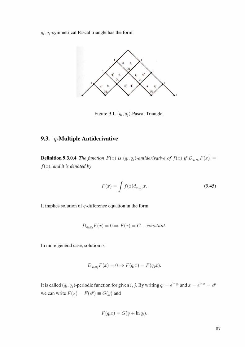
qi, qj-symmetrical Pascal triangle has the form:

Figure 9.1. (qi, qj)-Pascal Triangle

9.3. q-Multiple Antiderivative

Definition 9.3.0.4 The function F (x) is (qi, qj)-antiderivative of f(x) if Dqi,qjF (x) =

f(x), and it is denoted by

F (x) =

∫f(x)dqi,qj

x. (9.45)

It implies solution of q-difference equation in the form

Dqi,qjF (x) = 0 ⇒ F (x) = C − constant.

In more general case, solution is

Dqi,qjF (x) = 0 ⇒ F (qix) = F (qjx).

It is called (qi, qj)-periodic function for given i, j. By writing qi = eln qi and x = eln x = ey

we can write F (x) = F (ey) ≡ G(y) and

F (qix) = G(y + ln qi).

87

Using condition of (qi, qj)-periodicity of F (x), we have

G(y + ln qi) = G(y + ln qj)

and if we denote y + ln qi = z, then we obtain

G(z) = G(z + lnqj

qi

),

which means that G(z) is standard periodic function

G(z) = G(z + t)

with period t = lnqj

qi.

Example: If we consider G(z) in the form of sin function, then for (qi, qj)-

periodic function we get

F (x) = sin

(2π

lnqj

qi

ln x

)= sin

(2π

ln qj − ln qi

ln x

).

Applying Dqi,qj-operator to this function, we obtain

Dqi,qjsin

(2π

ln qj − ln qi

ln x

)= 0,

which proves that

F (x) = sin

(2π

lnqj

qi

ln x

)

is (qi, qj) periodic function.

Suppose f(x) is an analytic function expandable to power series f(x) =∑∞

k=0 akxk,

88

then f(x) has (qi, qj)- antiderivative in the following form

∫f(x)dqi,qj

x =∞∑

k=0

akxk+1

[k + 1]qi,qj

+ C,

where C-constant.

9.3.1. q-Periodic Functions and Euler Equation

The Euler differential equation

x2 d2y

dx2+ x

dy

dx+ ω2y = 0, (9.46)

by substitution x = et and

xd

dx=

d

dt,

transforms to harmonic oscillator equation

d2y

dt2+ ω2y = 0. (9.47)

Solution of the last equation

y(t) = Ae±iωt

implies solution of the Euler equation

y(x) = Ae±iω ln x.

89

This function is q-periodic function y(qx) = y(x) with q = e2πω . So the above results we

can summaries as : The Euler differential equation

x2 d2y

dx2+ x

dy

dx+

4π2

(ln q)2y = 0 (9.48)

has the general solution

y(x) = A cos

(2π

ln qln x

)+ B sin

(2π

ln qln x

),

or

y(x) = A cos(2π logq x

)+ B sin

(2π logq x

),

which is q-periodic (y(qx) = y(x)), and as follows Dqy(x) = 0.

9.4. q-Multiple Jackson Integral

Here we construct the q-multiple Jackson integral which gives us q-antiderivative

F (x) of an arbitrary function f(x). For this we write the derivative operator Dqi,qjin

terms of Mqi-operator defined by Mqi

F (x) = F (qix). From the definition of q derivative

we have

Dqi,qjF (x) =

1

(qi − qj)x(Mqi

−Mqj)F (x) = f(x), (9.49)

then the q-antiderivative is

F (x) = (Mqi−Mqj

)−1(qi − qj)xf(x). (9.50)

90

Now we find the inverse of (Mqi−Mqj

). We have

M−1qi

f(x) = f(1

qi

x) = M 1qi

,

therefore M−1qi

is inverse operator of Mqi. Then

Mqi−Mqj

= Mqi

(1− Mqj

Mqi

)= Mqi

(1−M−1

qiMqi

)

= Mqi

(1−M qj

qi

), (9.51)

and

(Mqi−Mqj

)−1 =

(1−M qj

qi

)−1

M−1qi

=

1

1−M qjqi

M 1

qi

=

(1 +

Mqj

Mqi

+

(Mqj

Mqi

)2

+ ...

)M 1

qi

= M 1qi

+ M qj

q2i

+ M q2j

q3i

+ ....

Substituting into (9.50), we obtain the q −multiple Jackson integral of f(x)

F (x) =

∫f

(x

qi

)d qj

qi

x = (qi − qj)∞∑

k=0

qkj x

qk+1i

f

(qkj x

qk+1i

). (9.52)

91

CHAPTER 10

NON-COMMUTATIVE Q-BINOMIAL FORMULAS

10.1. Gauss’s Binomial Formula

The Newton’s Binomial Formula for positive integer n is given in the following

form

(x + y)n =n∑

k=0

(n

k

)xn−kyk, (10.1)

where

(n

k

)=

n!

k!(n− k)!

denotes the corresponding binomial coefficients. And these binomial coefficients appear

as the entries of Pascal’s Triangle.

To obtain the q-analogue of Binomial formula (Kac & Cheung, 2002), one con-

siders function f(x) = (x + a)nq , and expand it around x = 0 to q-Taylor’s series . By

using notation

(x + a)nq ≡ (x + a)(x + qa)(x + q2a)...(x + qn−1a), n = 1, 2, .. (10.2)

and next calculations

(x + a)n−kq |(x=0)= q

(n−k)(n−k−1)2 an−k,

(Dkq f)(x) = [n]q[n− 1]q...[n− k + 1]q(x + a)n−k

q , (10.3)

92

we get the q- Taylor’s formula as

(x + a)nq =

n∑

k=0

[n

k

]

q

q(n−k)(n−k−1)

2 an−kxk. (10.4)

From the symmetry of q- binomial coefficients[nk

]q

=[

nn−k

]q

the above expression may

be rewritten as

(x + a)nq =

n∑

k=0

[n

k

]

q

qk(k−1)

2 xn−kak, (10.5)

which is called Gauss’s Binomial formula for commutative x and a (xa = ax).

Here we propose alternative way to obtain the above result, without using q-Taylor

formula (In the next section we apply the same method for new case of Q-commutative q-

binomial formula). It is based on solving the first order linear partial difference equation.

Suppose the Gauss’s Binomial formula (10.5) can be written in the following polynomial

form

(x + a)nq =

n∑j=0

n

j

q

xjan−j, (10.6)

with unknown coefficients

nj

q. So, by induction

(x + a)n+1q = (x + a)n

q (x + qna)

=n∑

j=0

n

j

q

xjan−j(x + qna)

=n∑

j=0

n

j

q

xj+1an−j +n∑

j=0

n

j

q

xjqnan−j+1.

By shifting j → j − 1 in the first sum, we obtain

n+1∑j=0

n + 1

j

q

xjan−j+1 =n+1∑j=1

n

j − 1

q

xjan−j+1 +n∑

j=0

n

j

q

xjqnan−j+1. (10.7)

93

From the above equalities we have

j = 0 ⇒

n + 1

0

q

= qn

n

0

q

,

j = n + 1 ⇒

n + 1

n + 1

q

=

n

n

q

,

j = k ⇒

n + 1

k

q

=

n

k − 1

q

+ qn

n

k

q

, 1 < k < n. (10.8)

It is convenient to put

n

b

q

= 0 if b < 0 and b > n.

Therefore we have the following equalities

n + 1

0

q

= qn

n

0

q

,

n + 1

n + 1

q

=

n

n

q

.

By recalling the known q-Pascal rule in terms of q-combinatorial coefficients

[n + 1

k

]

q

=

[n

k − 1

]

q

+ qk

[n

k

]

q

, (10.9)

we try to find the unknown combinatorial coefficients

nk

q

in terms of known q- combi-

natorial coefficients[nk

]q

with multiplying factor q in power of unknown function S(n, k)

n

k

q

= qS(n,k)

[n

k

]

q

. (10.10)

Substituting the above Ansatz into the recursion formula (10.8) and using the q-Pascal

94

rule (10.9), we obtain the following relation

qS(n+1,k)

[n

k − 1

]

q

+ qS(n+1,k)+k

[n

k

]

q

= qS(n,k−1)

[n

k − 1

]

q

+ qS(n,k)+n

[n

k − 1

]

q

.

By equating coefficients with the same power of q, we obtain the system of the first order

linear partial difference equations (h = 1)

S(n + 1, k) = S(n, k − 1) ⇒ DnS(n, k) = −DkS(n, k − 1),

S(n + 1, k) = S(n, k) + n− k ⇒ DnS(n, k) = n− k,

with initial conditions

S(0, 0) = S(1, 0) = S(1, 1) = 0, (k = 0, 1, ..., n),

where

Dhxf(x, y) = f(x + h, y)− f(x, y), Dh

yf(x, y) = f(x, y + h)− f(x, y).

Solution of the above system is found in the form (see Appendix C)

S(n, k) =(n− k)(n− k − 1)

2.

Hence,

n

k

q

= q(n−k)(n−k−1)

2

[n

k

]

q

. (10.11)

Then, by substituting into expansion (10.6), we come to Gauss’s Binomial formula for

commutative x and a (xa = ax).

95

10.2. Non-commutative Binomial Formula

For q-commutative x and y (yx = qxy), where q is a number, commutating with

x and y; xq = qx and yq = qy, we have the non-commutative Binomial formula

(x + y)n =n∑

k=0

[n

k

]

q

xkyn−k. (10.12)

It can be proved by mathematical induction (see for example Kac & Chung, 2002).

10.3. Q-commutative q-Binomial Formula

In this section we construct the q- Binomial formula for non-commutative x and y,

in the special case when they are Q-commutative (yx = Qxy) (Pashaev & Nalci, 2011d).

Firstly, we note that in notation of q-binomial we have the product

(x + y)nq = (x + y)(x + qy)(x + q2y)...(x + qn−1y), n = 1, 2, .. (10.13)

which we now apply to the noncommutative operators x and y, so that we should distin-

guish the direction of multiplication. So we have following notation for two cases

(x + y)n<q ≡ (x + y)(x + qy)(x + q2y)...(x + qn−1y) (10.14)

and

(x + y)n>q ≡ (x + qn−1y)...(x + qy)(x + y). (10.15)

Now we like to find expansion of these q-polynomials in terms of x and y powers. Sup-

96

pose we have the following expansion

(x + y)n<q =

n∑

k=0

n

k

Q,q

xn−kyk, (10.16)

where

(x + y)n<q = (x + y)(x + qy)(x + q2y)...(x + qn−1y),

and

nk

Q,q

- denote unknown coefficients, depending on k, n, q and Q. Then,

(x + y)n+1q = (x + y)n

q (x + qny).

Expanding both sides

n+1∑

k=0

n + 1

k

Q,q

xn−k+1yk =n∑

k=0

n

k

Q,q

xn−kyk(x + qny)

=n∑

k=0

n

k

Q,q

xn−kykx +n∑

k=0

n

k

Q,q

qnxn−kyk+1

=n∑

k=0

n

k

Q,q

Qkxn−k+1yk +n∑

k=0

n

k

Q,q

qnxn−kyk+1

=n∑

k=0

n

k

Q,q

Qkxn−k+1yk +n+1∑

k=1

n

k − 1

Q,q

qnxn−k+1yk

From the above equality we have the following recursion formulas :

k = 0 ⇒

n + 1

0

Q,q

=

n

0

Q,q

,

k = n + 1 ⇒

n + 1

n + 1

Q,q

= qn

n

n

Q,q

,

1 ≤ k ≤ n ⇒

n + 1

k

Q,q

= Qk

n

k

Q,q

+ qn

n

k − 1

Q,q

, (10.17)

97

where convenient to choose

n

b

Q,q

= 0 if b < 0 and b > n.

Suppose the unknown binomial coefficient factor

nk

Q,q

can be written in terms of the

known combinatorial coefficient[nk

]Q,q

with multiplication factor as

n

k

Q,q

= qt(n,k)

[n

k

]

Q,q

, (10.18)

where[nk

]Q,q

is (q,Q)- combinatorial coefficient with [n]Q,q = Qn−qn

Q−q(see section 9.2).

Substituting this relation to (10.17) and using (9.43), (9.44) we have following expression

Qkqt(n+1,k)

[n

k

]

Q,q

+ qn+1−k+t(n+1,k)

[n

k − 1

]

Q,q

= Qkqt(n,k)

[n

k

]

Q,q

+ qn+t(n,k−1)

[n

k − 1

]

Q,q

By equating terms with the same power of q and Q, we obtain two difference equations

t(n + 1, k) = t(n, k)

t(n, k) = t(n, k − 1) + k − 1 (10.19)

with the initial conditions

t(0, 0) = t(1, 0) = t(1, 1) = 0. (10.20)

Solution of this first order system of linear difference equations gives (see Appendix C)

t(n, k) =k(k − 1)

2. (10.21)

98

Hence,we obtain the q- Binomial formula for Q-commutative x and y in the form

(x + y)n<q =

n∑

k=0

[n

k

]

Q,q

qk(k−1)

2 xn−kyk, (10.22)

where yx = Qxy, and

[n

k

]

Q,q

=[n]Q,q!

[n− k]Q,q![k]Q,q!, [n]Q,q =

Qn − qn

Q− q.

Figure 10.1. Q-commutative q-Pascal triangle

It is instructive now to prove this Binomial formula by using mathematical induc-

tion. We have

(x + y)n+1q = (x + y)n

q (x + qny)

=n∑

k=0

[n

k

]

Q,q

qk(k−1)

2 xn−kyk(x + qny)

=n∑

k=0

[n

k

]

Q,q

qk(k−1)

2 xn−kykx +n∑

k=0

[n

k

]

Q,q

qk(k−1)

2 qnxn−kyk+1.

From the Q− commutativity relation yx = Qxy, we get ykx = Qkxyk and the above

99

expression is written as follows

(x + y)n+1q =

n∑

k=0

[n

k

]

Q,q

qk(k−1)

2 Qkxn−k+1yk +n∑

k=0

[n

k

]

Q,q

qk(k−1)

2 qnxn−kyk+1

=n∑

k=0

[n

k

]

Q,q

qk(k−1)

2 Qkxn−k+1yk +n+1∑

k=1

[n

k − 1

]

Q,q

q(k−1)(k−2)

2 qnxn−k+1yk

=

[n

0

]

Q,q

xn+1 +

[n

n

]

Q,q

qn(n+1)

2 yn+1

+n∑

k=1

([n

k

]

Q,q

qk(k−1)

2 Qk +

[n

k − 1

]

Q,q

q(k−1)(k−2)

2 qn

)xn−k+1yk. (10.23)

In Pascal rule for binomial coefficients (9.44) by choosing qi = Q and qj = q we have the

following relation

Qk

[n

k

]

Q,q

=

[n + 1

k

]

Q,q

− qn+1−k

[n

k − 1

]

Q,q

.

By substituting this relation into equation (10.23)we have desired result

(x + y)n+1q =

[n

0

]

Q,q

xn+1 +

[n

n

]

Q,q

qn(n+1)

2 yn+1 +n∑

k=1

[n

k

]

Q,q

qk(k−1)

2 xn−k+1yk

=n+1∑

k=0

[n + 1

k

]

Q,q

qk(k−1)

2 xn−k+1yk. (10.24)

Example: Consider the Q- derivative operator DQ =MQ−1

x(Q−1)with Q-dilatation

operator MQ = Qx ddx operators. These operators are Q-commutative

DQMQ = QMQDQ.

100

Then we have expansion

(MQ + DQ)n<q = (MQ + DQ)(MQ + qDQ)(MQ + q2DQ)...(MQ + qn−1DQ)

=n∑

k=0

[n

k

]

Q,q

qk(k−1)

2 Mn−kQ Dk

Q. (10.25)

The above result shows that Q-commutative q-binomials are expressed in terms

of our (q,Q) numbers, introduced in Section 9. Then we have next generalization of this

formula. Let operators x and y are qi commutative yx = qjxy, then

(x + y)n<qi

=n∑

k=0

[n

k

]

qi,qj

qi

k(k−1)2 xn−kyk, (10.26)

where[nk

]qi,qj

are combinatorial coefficients .

Example: The unitary operator D(α) = eαa+−αa for Heisenberg-Weyl group is

generating operator for Coherent states

|α >= D(α)|0〉,

where α is complex parameter. These operators satisfy relation

D(α)D(β) = e2i=(αβ)D(β)D(α),

hence they are Q-commutative with Q = e2i=(αβ). Then we have next operator q-Binomial

expansion

(D(β) + D(α))n<q =

n∑

k=0

[n

k

]

Q,q

qk(k−1)

2 Dn−k(β)Dk(α). (10.27)

101

If we apply this expansion to vacuum state |0〉, then we get

(D(β) + D(α))n<q |0〉 =

n∑

k=0

[n

k

]

Q,q

qk(k−1)

2 Dn−k(β)|kα〉

=n∑

k=0

[n

k

]

Q,q

qk(k−1)

2 eiδ|(n− k)β + kα〉, (10.28)

where

δ = 2= [(n− k)kαβ

].

Proposition 10.3.0.1 Above we have derived Q-commutative (10.14) q-binomial formula

for ordered product < q. Now we like to construct similar formula for opposite ordered

product > q (10.15). The following relation for two different ordered products is valid

N∏

k=0

(x + qky)<q =N∏

k=0

(x + QN−2kqky)>q, (10.29)

where yx = Qxy and

N∏

k=0

(x + qky)<q = (x + y)(x + qy)(x + q2y)...(x + qNy) = (x + y)N+1<q ,

N∏

k=0

(x + QN−2kqky)>q = (x + qNy)(x + qN−1y)...(x + qy)(x + y).

Proof 10.3.0.2 This formula can be proved by the method of mathematical induction.

N = 1 ⇒1∏

k=0

(x + qky)<q = (x + y)(x + qy) = x2 + qQ−1yx + Qxy + qy2

= (x + Q−1qy)(x + Qy) =1∏

k=0

(x + Q1−2kqky)>q

and we suppose that the formula is true for some N. Let us show that it is also valid for

102

N + 1 :

N+1∏

k=0

(x + qky)<q =N∏

k=0

(x + qky)<q(x + qN+1y)

=N∏

k=0

(x + QN−2kqky)>q(x + qN+1y)

= (x + Q−NqNy)...(x + Q(N−2)qy)(x + QNy)(x + qN+1y).

By using equality

(x + qmy)(x + qky) = (x + Q−1qky)(x + Qqmy),

we move the last term to the left-end by commutating with every term of the product

N+1∏

k=0

(x + qky)<q = (x + Q−NqNy)...(x + Q(N−2)qy)(x + Q−1qN+1y)(x + QN+1y)

= (x + Q−NqNy)...(x + Q−2qN+1y)(x + Q(N−1)qy)(x + QN+1y)

= ...

= (x + Q−(N+1)qN+1y)(x + Q−(N−1)qNy)...(x + QN+1y)

=N+1∏

k=0

(x + QN+1−2kqky)>q.

Proposition 10.3.0.3 For q = 1 we have the following relation

(x + y)n = (x + y)n<Q

, (10.30)

where

(x + y)n<Q

= (x + Q−(n−1)y)(x + Q−(n−3)y)...(x + Q(n−3)y)(x + Q(n−1)y)

is non-commutative binomial in symmetrical calculus case.

103

Proof 10.3.0.4 By mathematical induction, for n = 1, it is obvious. Suppose we have

(x + y)n = (x + y)n<Q

,

for arbitrary n. Then for n + 1 we have

(x + y)n+1 = (x + y)n(x + y) = (x + y)n<Q

(x + y)

= (x + Q−(n−1))(x + Q−(n−3))...(x + Q(n−3))(x + Q(n−1))(x + y)

= (x + Q−(n−1))(x + Q−(n−3))...(x + Q(n−3))(x + Q−1y)(x + Q(n))

= (x + Q−(n−1))(x + Q−(n−3))...(x + Q−2y)(x + Q(n−2))(x + Q(n))

= ...

= (x + Q−n)(x + Q−(n−2))...(x + Q(n−2))(x + Qn) = (x + y)n+1

<Q.

We summarize our results in the next q-binomial formula for Q-commutative op-

erators x and y:

(x + y)N<q =

N−1∏

k=0

(x + qky)<q = (x + y)(x + qy)(x + q2y)...(x + qN−1y)

=N∑

k=0

[N

k

]

q,Q

qk(k−1)

2 xn−kyk, (10.31)

where yx = Qxy.

Proposition 10.3.0.5 Two opposite ordered q-binomials are related by formula

(x + y)N<q = (x + QN−1y)N

> q

Q2, (10.32)

where yx = Qxy.

104

Proof 10.3.0.6 From equation (10.29) we have

N∏

k=0

(x + qky)<q =N∏

k=0

(x + QN−2kqky)>q =N∏

k=0

(x + (q

Q2)kQNy)>q = (x + QNy)N+1

> q

Q2;

(x + y)N+1<q = (x + QNy)N+1

> q

Q2⇒ (x + y)N

<q = (x + QN−1y)N> q

Q2.

Proposition 10.3.0.7 For yx = Qxy we obtain the following relation

(x + y)N>q =

N−1∏

k=0

(x + qky)>q =N∑

k=0

[N

k

]

qQ2,Q

(qQ2)k(k−1)

2 xN−k

(y

QN−1

)k

. (10.33)

Proof 10.3.0.8 We start from relation between direction of two multiplication rules (10.29)

N−1∏

k=0

(x + qky)<q =N−1∏

k=0

(x + QN−1−2kqky)>q

=N−1∏

k=0

(x + (q

Q2)kQN−1y)>q. (10.34)

By choosing QN−1y ≡ z ⇒ y = zQN−1 , the above equation becomes

N−1∏

k=0

(x +

(q

Q2

)k

z

)

>q

=N−1∏

k=0

(x + qk z

QN−1

)

<q

.

Let us call qQ2 ≡ q1, then according to Proposition 10.3.05

N−1∏

k=0

(x + qk1z)>q1 = (x + z)N

>q1=

N−1∏

k=0

(x + (q1Q

2)k z

QN−1

)=

(x +

z

QN−1

)N

<q1Q2

=N∑

k=0

[N

k

]

q1Q2,Q

(q1Q2)

k(k−1)2 xN−k

(z

QN−1

)k

. (10.35)

105

Relation yx = Qxy implies zx = Qxz, this is why, if we replace q1 → q and z → y, we

obtain the required result.

Finally, q-Binomial formulas for Q-commutative operators x and y with different order

are summarized in equations (10.31) and (10.33).

In the next section we show that all known binomial formulas like Gauss Binomial

formula etc. are particular cases of our non-commutative binomial formula.

10.3.1. Special Cases

Let us consider some particular cases of this generalized Q commutative q- Bino-

mial formula:

(i) for Q = 1, which means commutative x and y, this formula becomes the

Gauss Binomial formula

(x + y)nq =

n∑

k=0

[n

k

]

q

qk(k−1)

2 xn−kyk,

where yx = xy.

(ii) for Q- commutative x and y (yx = Qxy) and q = 1 we have Non-commutative

Binomial formula

(x + y)n =n∑

k=0

[n

k

]

Q

xn−kyk.

(iii) for Q = 1q, we obtain the symmetrical binomial formula

(x + y)nq =

n∑

k=0

[n

k

]

q

qk(k−1)

2 xn−kyk,

where yx = 1qxy.

(iv) for q = Q ⇒ limQ→q[n]q,q = nqn−1, and the formula transforms to the

106

following one

(x + y)nq =

n∑

k=0

(n

k

)qk(n− k+1

2)xn−kyk,

where(

nk

)= n!

(n−k)!k!- standard Newton binomials.

(v) By choosing q = − 1ϕ

and Q = ϕ, where ϕ is the Golden ratio, we obtain the

Binet-Fibonacci Binomial formula for Golden Ratio non-commutative plane (yx = ϕxy)

(Pashaev and Nalci, 2011a)

(x + y)n− 1

ϕ=

n∑

k=0

[n

k

]

ϕ,− 1ϕ

(− 1

ϕ)

k(k−1)2 xn−kyk

=n∑

k=0

Fn!

Fk!Fn−k!

(− 1

ϕ

) k(k−1)2

xn−kyk, (10.36)

where Fn are Fibonacci numbers, and q-binomial coefficients become Fibonomial.

10.3.2. q, Q- Binomial Formula

The above formulas we can compare with the one appearing from general com-

mutative multiple binomial formula. If we choose qi = q and qj = Q in (qi, qj) multiple

binomial formula (9.29), the following formula may obtained

(x + y)nq,Q =

n∑

k=0

[n

k

]

q,Q

(qQ)k(k−1)

2 xn−kyk,

where yx = xy.

107

10.3.3. q-Function of Non-commutative Variables

In Chapter 12 we introduce q-function of two variables. If

f(x) =∞∑

n=0

cnxn,

then q-function of two variables x and y is defined as

f(x + y)q =∞∑

n=0

cn(x + y)nq . (10.37)

We use these functions for definition of q-analytic functions and q-traveling waves. If

we take into account non-commutative binomial formulas derived in this section we

can extend our results from the Chapter 12 to the q-function of non-commutative (Q-

commutative) variables x and y. This why non-commutative q- analytic functions and

non-commutative q-traveling waves could be derived.

As an example below we briefly consider case of q-exponential function.

Definition 10.3.3.1 (q, Q) analogues of exponential function are defined as

eq,Q(x) ≡∞∑

n=0

1

[n]q,Q!xn,

Eq,Q(x) ≡∞∑

n=0

1

[n]q,Q!q

n(n−1)2 xn. (10.38)

Proposition 10.3.3.2 For Q-commutative operators x and y, (yx = Qxy), we have the

following factorization for q− exponential function eq,Q,

eq,Q(x + y)<q = eq,Q(x)Eq,Q(y),

where

108

eq,Q(x) ≡∞∑

n=0

1

[n]q,Q!xn,

Eq,Q(x) ≡∞∑

n=0

1

[n]q,Q!q

n(n−1)2 xn.

Proof 10.3.3.3

eq,Q(x + y)<q =∞∑

N=0

(x + y)N<q

[N ]q,Q!

=∞∑

N=0

1

[N ]q,Q!

N∑

k=0

[N

k

]

q,Q

qk(k−1)

2 xN−kyk

=∞∑

N=0

N∑

k=0

1

[N − k]q,Q![k]q,Q!q

k(k−1)2 xN−kyk.

By choosing N − k ≡ s,

eq,Q(x + y)<q =

( ∞∑s=0

1

[s]q,Q!xs

)( ∞∑

k=0

1

[k]q,Q!q

k(k−1)2 yk

)

= eq,Q(x)Eq,Q(y). (10.39)

109

CHAPTER 11

Q-QUANTUM HARMONIC OSCILLATOR

As an application of multiple q calculus developed in Chapter 9, here we study

quantum oscillator, deformed by two parameters q and Q. Different types of q-deformation

for quantum oscillator where intensively studied in a several papers. We will mention

here only most important papers: for non-symmetric oscillator (Arik & Coon, 1976),

for the symmetrical one (Biedenharn, 1989), (Macfarlane, 1989), and for generic (p,q)

(Chakrabarti & Jagannathan, 1991) and in (Arik et al., 1992).

11.1. Quantum Harmonic Oscillator

We consider simple harmonic oscillator with mass m and with spring constant k.

The motion is governed by Hooke’s law and Newton’s equation

F = −kx = md2x

dt2,

which can be written as

d2x

dt2+ ω2x = 0, (11.1)

where ω ≡√

km

is the angular frequency of oscillator.

The general solution is

x(t) = A sin(ωt) + B cos(ωt)

and the potential energy stored in a simple Harmonic oscillator at position x is

V (x) =1

2kx2.

110

For quantum oscillator in Schrodinger picture we have to solve the Schrodinger equation

with potential

V (x) =1

2mω2x2.

Then the time-independent Schrodinger equation for harmonic oscillator is written as

− ~2m

d2ψ

dx2+

1

2mω2x2ψ = Eψ. (11.2)

The above equation in terms of the momentum operator p ≡ ~i

ddx

and the position operator

x is

1

2m[p2 + (mωx)2]ψ = Eψ. (11.3)

These operators satisfy the canonical commutation relation [x, p] = i~, where the com-

mutator of operators A and B is [A,B] ≡ AB −BA. The basic Hamiltonian

H =1

2m[p2 + (mωx)2]. (11.4)

in terms of annihilation and creation operators

a =

√1

2~mω(ip + mωx),

a+ =

√1

2~mω(−ip + mωx), (11.5)

can be written as

H = ~ω(a+a +1

2).

The commutation relation [x, p] = i~ in terms of a and a+ becomes

[a, a+] = 1. (11.6)

The number operator

N = a+a

111

which is obviously Hermitian, satisfies the following commutation relations

[a, a+] = 1, [N, a] = −a, [N, a+] = a+. (11.7)

From (11.6) it is easy to get

aa+ = N + 1.

Then Hamiltonian expressed in terms of N is

H = ~ω(N +1

2).

The Schrodinger equation (11.2) for the Harmonic oscillator can also be written in terms

of a and a+ in the form

~ω(

a+a +1

2

)ψ = Eψ.

For eigenstates N |n〉 = n|n〉, we get the energy levels as

En =

(n +

1

2

)~ω, (n = 0, 1, 2, 3, ...).

As a result of commutation relations, we have

Na+|n〉 =([N, a+] + a+N

) |n〉 = a+|n〉+ a+N |n〉 = (n + 1)a+|n〉 (11.8)

Na|n〉 = ([N, a] + aN) |n〉 = −a|n〉+ aN |n〉 = (n− 1)a|n〉 (11.9)

112

and

a+|n〉 =√

n + 1|n + 1〉 (11.10)

a|n〉 =√

n|n− 1〉. (11.11)

The vacuum state is defined by

a|0〉 = 0,

which is the minimum energy state with eigenvalue

E0 =1

2~ω.

Applying the creation operator a+ n times to the ground state |0〉, we obtain all

eigenstates of the Hamiltonian in the form

|n〉 =

((a+)n

√n!

)|0〉. (11.12)

The energy eigenfuctions in position space are found by starting with the ground

state a|0〉 = 0

〈x|a|0〉 =1√

2~mω〈x|ip + mωx|0〉

=1√

2~mω

(~

mω

d

dx+ x

)〈x′|0〉 = 0

~mω

dΨ0

dx+ xΨ0 = 0

Ψ0 = Ae−mω2~ x2

.

By normalizing Ψ0

1 = |A|2∫ ∞

−∞e−

mω~ x2

dx,

113

we obtain

A2 =

√mω

π~.

So the ground state of the quantum harmonic oscillator is

Ψ0(x) =(mω

π~

)1/4

e−mω~ x2

. (11.13)

Hence, the excited states, increasing the energy by ~ω with each step, are constructed by

applying the creation operator repeatedly to the ground state as follows :

Ψn(x) = An(a+)nΨ0(x) =(mω

π~

)1/4 1√2~mω

(− ~

mω

d

dx+ x

)n

e−mω~ x2

(11.14)

with the energy spectrum

En =

(n +

1

2

)~ω (11.15)

where n = 0, 1, 2, ...

11.2. (qi, qj)-Quantum Harmonic Oscillator

In this section, we consider the general (qi, qj)-analogue of quantum harmonic

oscillator for N = 2. Such type of oscillators for two basis q, p were constructed by

(Chakrabarti & Jagannathan, 1991) and q1, q2 basis by (Arik et al., 1992). Then, we

consider the special cases of this harmonic oscillator as non-symmetrical, symmetrical

and Fibonacci cases.

Firstly, we define the q-bosonic creation operator a+q , its hermitian conjugate the q-

bosonic annihilation operator aq and the boson vacuum state |0〉i,j defined by aq|0〉i,j = 0.

(in following we skip indices i, j for operators a+q , aq.)

114

Instead of the Heisenberg (Lie) algebra ,we postulate the algebraic relation

aqa+q − qia

+q aq = qN

j , (11.16)

or by using the symmetry property of the (qi, qj)-number under the exchange qi ↔ qj we

have another algebraic relation

aqa+q − qja

+q aq = qN

i , (11.17)

where N is the hermitian number operator and qi, qj are deformation parameters. The

bosonic q-oscillator is defined by three operators a+q , aq and N which satisfy the commu-

tation relations:

[N, a+q ] = a+

q , [N, aq] = −aq. (11.18)

The algebra (11.16)-(11.18) is the (qi, qj)-analogue generalization of the Heisenberg al-

gebra. In the limiting case qi → 1 and qj → 1, these algebraic relations reduce to the

standard Heisenberg algebraic relations .

By using definition of (qi, qj)-number operator

[N ]i,j =qNi − qN

j

qi − qj

for qi 6= qj, we find following equalities

[N + 1]i,j − qi[N ]i,j = qNj , (11.19)

[N + 1]i,j − qj[N ]i,j = qNi . (11.20)

If we choose qi = qj, then the q-number operator is [N ]qi,qj= NqN−1

i . By com-

115

parison the above operator relations with algebraic relations (11.16) and (11.17) we have

a+q aq = [N ]i,j, aqa

+q = [N + 1]i,j.

Here we should note that the number operator N is not equal to a+q aq as in ordinary case.

The basis of the Fock space is defined by repeated action of the creation operator

a+q on the vacuum state |0〉i,j , which is annihilated by aq|0〉i,j = 0

|n〉i,j =(a+

q )n|0〉i,j√[n]i,j!

. (11.21)

And the action of the operators on this basis is given by

N |n〉i,j = n|n〉i,j,[N ]i,j|n〉i,j = [n]i,j|n〉i,j,a+

q |n〉i,j =√

[n + 1]i,j|n + 1〉i,j,

aq|n〉i,j =√

[n]i,j|n− 1〉i,j.

(Proofs of these actions are in Appendix D)

Proposition 11.2.0.4

[Nn, a+q ] = Nn − (N − 1)na+

q . (11.22)

Proof 11.2.0.5 It is easy to prove by induction. (See Appendix D)

Proposition 11.2.0.6

[[N ]i,j, a

+q

]= [N ]i,j − [N − 1]i,ja+

q

= a+q [N + 1]i,j − [N ]i,j. (11.23)

116

Proof 11.2.0.7 For the first equality we use definition of q−number operator.

[N ]i,j =qNi − qN

j

qi − qj

=1

qi − qj

(eN ln qi − e−N ln qj

)

=1

qi − qj

∞∑

k=0

((ln qi)

kNk

k!− (ln qj)

kNk

k!

)

=1

qi − qj

∞∑

k=0

(ln qi)k − (ln qj)

k

k!Nk, (11.24)

[[N ]i,j, a

+q

]=

1

qi − qj

∞∑

k=0

(ln qi)k − (ln qj)

k

k![Nk, a+

q ]

=1

qi − qj

∞∑

k=0

(ln qi)k − (ln qj)

k

k!Nk − (N − 1)ka+

q

=1

qi − qj

(eN ln qi − e(N−1) ln qi − eN ln qj + e(N−1) ln qj

)a+

q

=1

qi − qj

(qNi − qN

j − (qN−1i − qN−1

j ))a+

q

= [N ]i,j − [N − 1]i,ja+q .

For second equality 11.23,we use the commutator properties :

[[N ]i,j, a

+q

]=

[a+

q aq, a+q

]= a+

q

[aq, a

+q

]= a+

q

(aqa

+q − a+

q aq

)

= a+q [N + 1]i,j − [N ]i,j.

Proposition 11.2.0.8 We have following equality for n = 0, 1, 2, ..

[[N ]ni,j, a+q ] = [N ]ni,j − [N − 1]ni,ja+

q (11.25)

Proof 11.2.0.9 By using mathematical induction to show the above equality is not diffi-

cult.

For n = 1 case : It is obviously true due to (11.23).

117

Suppose this equality is true for n

[[N ]ni,j, a

+q

]= [N ]ni,j − [N − 1]ni,ja+

q

we should prove it for n + 1,

[[N ]n+1

i,j , a+q

]= [N ]ni,j

[[N ]i,j, a

+q

]+

[[N ]ni,j, a

+q

][N ]i,j

= [N ]ni,j[N ]i,j − [N − 1]i,ja+q + [N ]ni,j − [N − 1]ni,ja+

q [N ]i,j

Using a+q [N ]i,j = [N − 1]i,ja

+q , we obtain the desired result

[[N ]n+1

i,j , a+q

]= [N ]n+1

i,j − [N − 1]n+1i,j a+

q . (11.26)

Corollary 11.2.0.10

Nna+q = a+

q (N + 1)n (11.27)

and

aqNn = (N + 1)naq (11.28)

Proof 11.2.0.11 By using the commutation relation and the equality (11.22)

[Nn, a+q ] = Nna+

q − a+q Nn = Nn − (N − 1)na+

q

we obtain

Nna+q = a+

q (N + 1)n.

118

And by taking the hermitian conjugate of this equation, we write

aqNn = (N + 1)naq.

Corollary 11.2.0.12 For any function expandable to power series (analytic) F (x) =∑∞

n=0 cnxn we have the following relation

[F ([N ]i,j), a+q ] = F ([N ]i,j)− F ([N − 1]i,j)a+

q

= a+q F ([N + 1]i,j)− F ([N ]i,j) (11.29)

and

a+q F ([N + 1]i,j) = F ([N ]i,j)a

+q (11.30)

or

F (N)a+q = a+

q F (N + 1) (11.31)

Proof 11.2.0.13

[F ([N ]i,j), a+q ] =

[ ∞∑n=0

cn[N ]ni,j, a+q

]=

∞∑n=0

cn

[[N ]ni,j, a

+q

]

=∞∑

n=0

cn[N ]ni,j − [N − 1]ni,ja+q

= F ([N ]i,j)− F ([N − 1]i,j)a+q (11.32)

[F ([N ]i,j), a+q ] = F [N ]i,ja

+q − a+

q F [N ]i,j = F ([N ]i,j)− F ([N − 1]i,j)a+q

119

As a result, we obtain

a+q F [N ]i,j = F [N − 1]i,ja

+q ,

a+q F [N + 1]i,j − a+

q F [N ]i,j = F [N ]i,ja+q − a+

q F [N ]i,j

= a+q (F [N + 1]i,j − F [N ]i,j) = [F ([N ]i,j), a

+q ].

If we use the definition of function of an operator

F (N)|n〉i,j = F (n)|n〉i,jF (N)a+

q |n〉i,j =√

[n + 1]i,jF (N)|n + 1〉i,j =√

[n + 1]i,jF (n + 1)|n + 1〉i,j,

and

a+q F (N + 1)|n〉i,j = a+

q F (n + 1)|n〉i,j =√

[n + 1]i,jF (n + 1)|n + 1〉i,j,

then we have equality

F (N)a+q = a+

q F (N + 1),

in a weak sense, i.e. it is valid on eigenstates |n〉i,j of number operator N. According to

above,we postulate that the relation (11.31) is valid for any function F.

Example: For negative power it gives

N−ka+q = a+

q (N + 1)−k.

Indeed,

NkN−ka+q = Nka+

q (N + 1)−k

a+q = a+

q (N + 1)k(N + 1)−k = a+q .

120

Now we find the normalization of (qi, qj)-boson state (11.21):

|n〉i,j =(a+

q )n|0〉i,j√[n]i,j!

, (11.33)

i,j〈n|n〉i,j =1

[n]i,j!i,j〈0|an

q (a+q )n|0〉i,j =

1

[n]i,j!i,j〈0|an−1

q aqa+q (a+

q )n−1|0〉i,j

=1

[n]i,j!i,j〈0|an−2

q aq[N + 1]i,ja+q (a+

q )n−2|0〉i,j

=1

[n]i,j!i,j〈0|an−2

q aqa+q [N + 2]i,j(a

+q )n−2|0〉i,j

=1

[n]i,j!i,j〈0|an−3

q aq[N + 1]i,j[N + 2]i,ja+q (a+

q )n−3|0〉i,j

=1

[n]i,j!i,j〈0|an−3

q aq[N + 1]i,ja+q [N + 3]i,j(a

+q )n−3|0〉i,j

=1

[n]i,j!i,j〈0|an−3

q aqa+q [N + 2]i,j[N + 3]i,j(a

+q )n−3|0〉i,j

...

=1

[n]i,j!i,j〈0|[N + 1]i,j[N + 2]i,j[N + 3]i,j...[N + n]i,j|0〉i,j

=1

[n]i,j![1]i,j[2]i,j...[n]i,j = 1. (11.34)

By introducing the position and momentum operators related to the (qi, qj)-bosonic

creation and annihilation operators

Xq =

√~

2mω(a+

q + aq)

Pq = i

√m~ω

2(a+

q − aq) (11.35)

we find Hamiltonian of the q-Harmonic Oscillator

Hq =P2

q

2m+

1

2mω2X2

q (11.36)

121

which can also be written as

Hq =~ω2

(aqa+q + a+

q aq). (11.37)

Its eigenvalues

Hq|n〉i,j = En|n〉i,j,

Hq|n〉i,j =~ω2

(aqa+q + a+

q aq)

=~ω2

([N ]i,j + [N + 1]i,j)|n〉i,j

=~ω2

([n]i,j + [n + 1]i,j)|n〉i,j (11.38)

give the energy spectrum

En =~ω2

([n]i,j + [n + 1]i,j), (11.39)

where n = 0, 1, 2, ... We note that these energy levels are not equally spaced for q 6= 1 ,

but the ground state energy still is the same ~ω2

.

Finally, we notice that the (qi, qj)-deformed boson operators a+q , aq can be ex-

pressed in the form

a+q = a+

√[N + 1]i,j

N + 1=

√[N ]i,j

Na+, (11.40)

aq =

√[N + 1]i,j

N + 1a = a

√[N ]i,j

N, (11.41)

where a+ and a are the creation and annihilation operators for quantum harmonic oscil-

lator. As a result of these relations, we can obtain the commutation relation between a+q

and aq as

[aq, a+q ] = aqa

+q − a+

q aq = [N + 1]i,j − [N ]i,j.

122

To compare n-particle states for both oscillators we consider next relations. From

(11.40)-(11.41) we have

(a+q )n =

(a+

√[N + 1]i,j

N + 1

)n

= a+

√[N + 1]i,j

N + 1a+

√[N + 1]i,j

N + 1...a+

√[N + 1]i,j

N + 1

= (a+)2

√[N + 2]i,j

N + 2

√[N + 1]i,j

N + 1a+

√[N + 1]i,j

N + 1...a+

√[N + 1]i,j

N + 1

= (a+)3

√[N + 3]i,j

N + 3

√[N + 2]i,j

N + 2

√[N + 1]i,j

N + 1...a+

√[N + 1]i,j

N + 1

= (a+)n

√[N + n]i,j

N + n...

[N + 2]i,j[N + 2]

[N + 1]i,j[N + 1]

= (a+)n

√[N + n]i,j!

[N ]i,j!

N !

(N + n)!(11.42)

And by taking the hermitian conjugate of this result we obtain

anq =

√[N + n]i,j!

[N ]i,j!

N !

(N + n)!an. (11.43)

Our next step is to show that the same set of eigenvectors |n〉 expands the whole Hilbert

space both for the standard harmonic oscillator and for its q−analogue. Firstly, we con-

sider the vacuum state |0〉 for ordinary quantum harmonic oscillator satisfies a|0〉 = 0,

and the vacuum state |0〉i,j for generic quantum harmonic oscillator satisfies aq|0〉i,j = 0.

From the relation (11.41) we write

aq|0〉i,j =

√[N + 1]i,j

N + 1a|0〉i,j = 0,

which gives that

a|0〉i,j = 0.

From another side , if a|0〉i,j = 0, it implies aq|0〉i,j = 0.

Therefore, the vacuum state |0〉 for ordinary oscillator is exactly the same for q− deformed

oscillator vacuum state |0〉 ≡ |0〉i,j. By applying the (a+q )n to the vacuum state |0〉i,j and

123

using the N |n〉i,j = n|n〉i,j

(a+q )n|0〉i,j = (a+)n

√[N + n]i,j!

[N ]i,j!

N !

(N + n)!|0〉i,j

=

√[n]i,j!

n!(a+

q )n|0〉 (11.44)

which implies that

|n〉i,j = |n〉.

As a result we found that both the standard and q− deformed harmonic oscillators have

the same set of eigenstates, but with different energy eigenvalues. If for standard oscillator

qi,j = 1 eigenstates are determined by positive integer numbers n; En = ~ω(n + 1

2

), then

for deformed oscillator they are given by q-deformed number [n]qi,qj; En = ~ω

2([n]i,j +

[n + 1]i,j).

11.2.1. Binet-Fibonacci Golden Oscillator and Fibonacci Sequence

As a new and interesting example of the (qi, qj) generic quantum harmonic oscil-

lator with N = 2, we consider the Binet-Fibonacci Golden harmonic oscillator (Pashaev

& Nalci, 2011a). Our Golden Harmonic oscillator is a particular case of so called gen-

eralized Fibonacci oscillator considered by (Arik et al., 1992) for arbitrary base q1, q2.

However Binet formula for Fibonacci numbers can be interpreted as a q-number with

base in the form of the Golden Ratio, and this base has many interesting properties. Due

to this and importance of the Golden Ratio in many phenomena, we will treat this special

case in all details.

To obtain the Golden harmonic oscillator, we choose (qi, qj) as roots of equation

x2 − x− 1 = 0, which qi = 1+√

52

≡ ϕ and qj = 1−√52

≡ ϕ′ = − 1ϕ

= 1− ϕ. The number

ϕ is called the Golden ratio (section).

Then, the Fibonacci sequence in Binet’s representation is the q-number

Fn =ϕn − ϕ′n

ϕ− ϕ′= [n]ϕ,ϕ′ ≡ [n]F ,

and due to addition rule the sequence Fn of Fibonacci numbers satisfies recurrence rela-

124

tion

Fn = Fn−1 + Fn−2,

with F0 = 0 and F1 = 1. First few Fibonacci numbers are

1, 1, 2, 3, 5, 8, 13, 21, ...

In the limit

limn→∞

F (n + 1)

F (n)= lim

n→∞

[n + 1]ϕ,− 1ϕ

[n]ϕ,− 1ϕ

= qi =1 +

√5

2≡ ϕ ≈ 1, 6180339887,

which is the Golden ratio.

For Binet-Fibonacci case, the algebraic relations (11.16) and (11.17) transform

into following form

bb+ − ϕb+b = (− 1

ϕ)N , (11.45)

bb+ +1

ϕb+b = ϕN . (11.46)

By using eigenvalues of the Number operator N |n〉F = n|n〉F ,

[N ]F |n〉F = FN |n〉F = [n]F |n〉F = Fn|n〉F

we get Fibonacci numbers as eigenvalues of operator [N ](or Fibonacci number operator).

The basis of the Fock space is defined by repeated action of the creation operator

b+ on the vacuum state, which is annihilated by b|0〉F = 0

|n〉F =(b+)n

√F1 · F2 · ...Fn

|0〉F , (11.47)

125

where [n]F ! = F1 · F2 · ...Fn.

The number operator N for Fibonacci case is written for two different forms ac-

cording to even or odd eigenstates N |n〉F = n|n〉F . For n = 2k, we get

N = logϕ

(√5

2FN +

√5

4F 2

N + 1

), (11.48)

and for n = 2k + 1,

N = logϕ

(√5

2FN −

√5

4F 2

N − 1

), (11.49)

where Fibonacci number operator is defined as

[N ]F =ϕN − (− 1

ϕ)

ϕ− (− 1ϕ)≡ FN .

As a result, the Fibonacci numbers are the example of (qi, qj) numbers with two basis and

one of the base is Golden Ratio. This is why we called the corresponding q− oscillator as

a Golden oscillator or Binet-Fibonacci Oscillator. The Hamiltonian for Golden oscillator

is written as a Fibonacci number operator

H =~ω2

(b+b + bb+) =~ω2

FN+2,

where bb+ = [N + 1]F = FN+1, b+b = [N ]F = FN . According to the Hamiltonian, the

energy spectrum of this oscillator is written in terms of Fibonacci numbers sequence,

En =~ω2

([n]F + [n + 1]F ) =~ω2

(Fn + Fn+1) =~ω2

Fn+2,

En =~ω2

Fn+2. (11.50)

126

Figure 11.1. Fibonacci tree for spectrum of Golden Oscillator

and satisfies the Fibonacci property

En+1 = En + En−1.

A first energy eigenvalue is

E0 =~ω2

F2 =~ω2

,

which is exactly the same ground state as in the ordinary case. The higher energy excited

127

states are given by Fibonacci sequence

E1 =~ω2

F3 = ~ω, E2 =3~ω2

, E3 =5~ω2

, ...

The difference between two consecutive energy levels of our oscillator is found as

4En = En+1 − En =~ω2

Fn+1.

Then the ratio of two successive energy levels En+1

Engives the Golden sequence, and for

the limiting case of higher excited states n →∞ it becomes the Golden ratio

limn→∞

En+1

En

= limn→∞

Fn+3

Fn+2

= limn→∞

[n + 3]α,β

[n + 2]α,β

=1 +

√5

2≈ 1, 6180339887.

This property of asymptotic states to relate each other by a Golden ratio, leads us to call

this oscillator as a Golden oscillator.

For this case we have the following relation between q- creation and annihilation

operators and standard creation and annihilation operators

b+ = a+

√FN+1

N + 1=

√FN

Na+

b =

√FN+1

N + 1a = a

√FN

N, (11.51)

where [a, a+] = 1.

11.2.2. Symmetrical q-Oscillator

For completeness here we review the important for quantum groups applications,

the symmetrical case (Biedenharn, 1989), (Macfarlane, 1989) as the special cases of

(qi, qj)− quantum harmonic oscillator.

For symmetrical case qi = q and qj = 1q

the algebraic relations (11.16) and (11.17)

128

transform into following form

aqa+q − qa+

q aq = q−N , (11.52)

or by using the invariance of the q-number under the exchange q ↔ q−1 we have another

algebraic relation

aqa+q − q−1a+

q aq = qN , (11.53)

where N is the Hermitian number operator and q is the deformation parameter. The

commutation relations satisfied by three operators a+q , aq and N are the same (11.18). By

using the definition of symmetric q-number operator we write following equalities

[N + 1]q − q[N ]q = q−N , (11.54)

[N + 1]q − q−1[N ]q = qN , (11.55)

where [x]q = qx−q−x

q−q−1 . By comparison the above operator relations with algebraic relations

(11.52) and (11.53) we have

a+q aq = [N ]q, aqa

+q = [N + 1]q.

In this special case, we find the number operator N in terms of [N ]q = a+q aq operator as

follows (Appendix D)

N = logq

[N ]q

q − q−1

2+

√([N ]q

q − q−1

2

)2

+ 1

(11.56)

or in the following form,

N =arcsinh([N]q sinh(ln q))

ln q. (11.57)

129

Like we did for generic case, the basis of the Fock space is defined by repeated

action of the creation operator a+q on the vacuum state, which is annihilated by aq|0〉q = 0

|n〉q =(a+

q )n|0〉q√[n]q!

. (11.58)

And the action of the operators on the basis are given by

N |n〉q = n|n〉q (11.59)

[N ]q|n〉q = [n]q|n〉q (11.60)

a+q |n〉q =

√[n + 1]q|n + 1〉q (11.61)

aq|n〉q =√

[n]q|n− 1〉q. (11.62)

The energy spectrum En, is written as

En =~ω2

([n]q + [n + 1]q), (11.63)

where n = 0, 1, 2, .. We notice that they are not equally spaced for q 6= 1 case. For

real q the energy spectrums increase more rapidly than the ordinary equidistant case. In

particular, for q = eα the energy spectrum is written in the following form

En =~ω2

sinh(α(n + 12))

sinh(α2)

.

For complex q where (q = eiα) is the phase factor and α is real, the eigenvalues of the

energy increase less rapidly than the ordinary case

En =~ω2

sin(α(n + 12))

sin(α2)

,

but the ground state still gives the same value 1/2.

In these two particular cases, in the limit q → 1 (α = 0) the ordinary expression for

130

energy spectrum

En = ~ω(

n +1

2

)

is obtained.

11.2.3. Non-symmetrical q-Oscillator

For non-symmetrical case qi = q and qj = 1 (Arik & Coon, 1976) we have the

following two algebraic relations

aqa+q − qa+

q aq = 1

and

aqa+q − a+

q aq = qN .

By using definition of non-symmetrical q− number we obtain

[N + 1]q − q[N ]q = 1

[N + 1]q − [N ]q = qN

where [x]q = qx−1q−1

. And we have

a+q aq = [N ]q, aqa

+q = [N + 1]q

The basis of the Fock space is

|n〉q =(a+

q )n|0〉q√[n]q!

. (11.64)

131

And the action of the operators on the basis is given by

N |n〉q = n|n〉q (11.65)

[N ]q|n〉q = [n]q|n〉q (11.66)

a+q |n〉q =

√[n + 1]q|n + 1〉q (11.67)

aq|n〉q =√

[n]q|n− 1〉q. (11.68)

The eigenvalues of energy are written in non-symmetrical q basis as follows

En =~ω2

([n]q + [n + 1]q) (11.69)

where n = 0, 1, 2, ..

From the values of energy spectrum we can note that for q > 1, the spectrum increases

more rapidly than the ordinary equidistant spectrum. In contrast, for 0 < q < 1 the

spectrum is increasing less rapidly than the ordinary equidistant case.

11.3. q-Deformed Quantum Angular Momentum

It is well known that algebra of angular momentum su(2) may be described in

terms of double oscillator representation, also known as the Schwinger representation

(Mattis, 1965). The pair of bosonic operators [ai, a+j ] = δij, (i, j = 1, 2) generates su(2)

algebra [Ji, Jj] = εijkJk, where J+ = J1 + iJ2 = a+1 a2, J− = J1 − iJ2 = a+

2 a1 and

J3 = 12(a+

1 a1 − a+2 a2).

Now by using pair of q− bosons we derive q− deformed quantum angular mo-

mentum algebra suq(2), such that for q → 1 it reduces to su(2) (Biedenharn, 1989),

(Macfarlane, 1989):

limq→1

suq(2) = su(2).

132

11.3.1. Double q-Boson Algebra Representation

In order to find this representation we consider two uncoupled q− oscillator sys-

tems : the q− creation and q− annihilation operators, denoted by b+1 and b1 for the first

system and b+2 and b2 for second one. We consider the algebraic relations among b+

a , ba

and Na

b1b+1 − qib

+1 b1 = qN1

j or b1b+1 − qjb

+1 b1 = qN1

i , (11.70)

and

b2b+2 − qib

+2 b2 = qN2

j or b2b+2 − qjb

+2 b2 = qN2

i , (11.71)

[Na, b

+a

]= b+

a ,

[Na, ba] = −ba,

where a = 1, 2, N1 is the hermitian number operator for the first quantum harmonic

system and N2 is also hermitian number operator for the second one which are defined by

N1 = a+1 a1 , N2 = a+

2 a2,

where [aa, a+b ] = δab.

In addition to these relations, any pair of operators between different oscillators

commute

[ba, b+b ] = [ba, bb] = [Na, Nb] = 0,

where a 6= b.

Commutativity of N1 and N2, implies that they have common eigenvector |n1, n2〉i,jwith eigenvalues n1 and n2 respectively. So, we can write the following eigenvalue equa-

133

tions for N1, N2

N1|n1, n2〉i,j = n1|n1, n2〉i,jN2|n1, n2〉i,j = n2|n1, n2〉i,j

and from the above equations we also write

[N1]i,j|n1, n2〉i,j =qN1i − qN1

j

qi − qj

|n1, n2〉i,j =qn1i − qn1

j

qi − qj

|n1, n2〉i,j = [n1]i,j|n1, n2〉i,j.

Similarly,

[N2]i,j|n1, n2〉i,j = [n2]i,j|n1, n2〉i,j,

where

[N1]i,j = b+1 b1, [N1 + 1]i,j = b1b

+1 , [N2]i,j = b+

2 b2, [N2 + 1]i,j = b2b+2 .

As a result of the commutation relations, we have

N1

(b+1 |n1, n2〉i,j

)=

(b+1 N1 + b+

1

) |n1, n2〉i,j = n1b+1 |n1, n2〉i,j + b+

1 |n1, n2〉i,j= (n1 + 1)

(b+1 |n1, n2〉i,j

). (11.72)

According to the above relation, vector b+1 |n1, n2〉i,j is also eigenket of N1 with eigenvalue

increased by one.Then, Equation (11.72) implies that b+1 |n1, n2〉i,j and |n1 + 1, n2〉i,j are

the same vectors with only difference in a complex constant

b+1 |n1, n2〉i,j = c|n1 + 1, n2〉i,j

134

fixed value of c is a constant. Then, from normalization condition we can find

〈n1, n2|b1b+1 |n1, n2〉i,j = |c|2〈n1 + 1, n2|n1 + 1, n2〉i,j

〈n1, n2|[N1 + 1]i,j|n1, n2〉i,j = [n1 + 1]i,j = |c|2,

so taking c to be real and positive, we eventually obtain

b+1 |n1, n2〉i,j =

√[n1 + 1]i,j|n1 + 1, n2〉i,j. (11.73)

For the q-creation and annihilation operators b+1 , b+

2 and b1, b2 correspondingly, action on

states|n1, n2〉i,j can be found as follows :

b+1 |n1, n2〉i,j =

√[n1 + 1]i,j |n1 + 1, n2〉i,j (11.74)

b+2 |n1, n2〉i,j =

√[n2 + 1]i,j |n1, n2 + 1〉i,j (11.75)

b1|n1, n2〉i,j =√

[n1]i,j |n1 − 1, n2〉i,j (11.76)

b2|n1, n2〉i,j =√

[n2]i,j |n1, n2 − 1〉i,j. (11.77)

The vacuum ket is defined by

b1|0, 0〉i,j = 0,

b2|0, 0〉i,j = 0.

By applying b+1 and b+

2 creation operators to the vacuum state |0, 0〉i,j we obtain the gen-

eral eigenvectors of N1, N2

|n1, n2〉i,j =(b+

1 )n1 (b+2 )n2

√[n1]i,j!

√[n2]i,j!

|0, 0〉i,j. (11.78)

By using the (qi, qj)- boson state, we can prove the normalization of state |n1, n2〉i,j in the

135

following way

i,j〈n1, n2|n1, n2〉i,j =〈0, 0|(b2)

n2(b1)n1(b+

1 )n1(b+2 )n2|0, 0〉

[n1]i,j![n2]i,j!.

And applying the relation (11.30), we calculate

1 =〈0, 0|(b2)

n2(b1)n1−1b1b

+1 (b+

1 )n1−1(b+2 )n2|0, 0〉

[n1]i,j![n2]i,j!

=〈0, 0|(b2)

n2(b1)n1−2b1[N1 + 1]i,jb

+1 (b+

1 )n1−2(b+2 )n2|0, 0〉

[n1]i,j![n2]i,j!

=〈0, 0|(b2)

n2(b1)n1−3b1[N1 + 1]i,j[N1 + 2]i,jb

+1 (b+

1 )n1−3(b+2 )n2|0, 0〉

[n1]i,j![n2]i,j!

=〈0, 0|(b2)

n2 [N1 + 1]i,j[N1 + 2]i,j...[N1 + n1]i,j(b+2 )n2|0, 0〉

[n1]i,j![n2]i,j!

=[1]i,j[2]i,j...[n1]i,j〈0, 0|(b2)

n2(b+2 )n2|0, 0〉

[n1]i,j![n2]i,j!

=〈0, 0|[N2 + 1]i,j[N2 + 2]i,j...[N2 + n2]i,j|0, 0〉

[n2]i,j!

=[1]i,j[2]i,j...[n2]i,j〈0, 0|0, 0〉

[n2]i,j!= 1.

11.3.2. su(qi,qj)(2) Angular Momentum Algebra

Now, by using operators b1, b+1 , b2, b

+2 we construct su(qi,qj)(2) algebra, which is

the (qi, qj)-multiple deformation of su(2). Firstly, we define (qi, qj) angular momentum

operators and corresponding algebra. Then from this algebra we construct the set of

eigenstates and eigenvalues for this angular momentum.

We define the following angular momentum operators :

Jq+ = ~ b+

1 b2 (11.79)

Jq− = ~ b+

2 b1 (11.80)

Jqz =

~2(N1 −N2) =

~2(b+

1 b1 − b+2 b2) = Jz, (11.81)

136

where b1, b2 are q-bosonic operators satisfying commutation relations (11.70), (11.71).

These operators satisfy the deformed angular momentum commutation relations :

[Jz, Jq+] = ~Jq

+ (11.82)

[Jz, Jq−] = −~Jq

− (11.83)

[Jq+, Jq

−] = ~2(qiqj)N2

[2

~Jz

]

i,j

= −~2(qiqj)N1

[−2

~Jz

]

i,j

(11.84)

where [Jz]i,j =qJzi −qJz

j

qi−qj.

The proves are as follows

1) [Jq+, Jq

−] = ~2b+1 b2 b+

2 b1 − b+2 b1 b+

1 b2= ~2qN2

j b+1 b1 + qib

+1 b1 b+

2 b2 − qN1j b+

2 b2 − qib+2 b2 b+

1 b1= ~2

(qN2j [N1]i,j − qN1

j [N2]i,j)

= ~2

(qN1i qN2

j − qN2i qN1

j

qi − qj

)

= ~2

((qiqj)

N2

(qN1−N2i − qN1−N2

j

qi − qj

))

= ~2

((qiqj)

N1

(qN2−N1j − qN2−N1

i

qi − qj

))

= ~2(qiqj)N2 [N1 −N2]i,j = −~2(qiqj)

N1 [N2 −N1]i,j

= ~2(qiqj)N2

[2

~Jz

]

i,j

= −~2(qiqj)N1

[−2

~Jz

]

i,j

,

where

[N1 −N2]i,j = −(qiqj)N1−N2 [N2 −N1]i,j.

137

2) [Jz, Jq+] =

~2

2[N1 −N2, b

+1 b2]

=~2

2

([N1, b

+1 b2]− [N2, b

+1 b2]

)

=~2

2

([N1, b

+1 ]b2 − b+

1 [N2, b2])

= ~Jq+. (11.85)

Hermitian conjugate of this relation gives

3) ([Jz, Jq+])† = [Jq

−, Jz] = −[Jz, Jq−] = ~Jq

−

so that we have

[Jq−, Jz] = −~Jq

−.

Now we construct eigenvalue problem for this (qi, qj) angular momentum operator

algebra. We have next proposition.

Proposition 11.3.2.1

[Jnz , Jq

+] = (Jnz − (Jz − 1)n) Jq

+. (11.86)

In more general case,

[f(Jz), Jq+] = (f(Jz)− f(Jz − 1)) J+

where f is function expandable to power series. We suppose that it is valid also for

arbitrary function f.

(Proof of this proposition is given in Appendix F)

138

The Casimir operator for this generic algebra (11.82)-(11.84) case is written as

Cq = (qiqj)−Jz

([Jz]i,j[Jz + 1]i,j + (qiqj)

−N2Jq−Jq

+

)

= (qiqj)−Jz

((qiqj)[Jz]i,j[Jz − 1]i,j + (qiqj)

−N2Jq+Jq

−)

where for simplicity we choose ~ = 1.

Due to this proposition, we can prove that [Cq, Jq±] = 0 and [Cq, Jq

z ] = 0. For

details of proof see (Appendix F). Commutativity of Cq and Jqz , implies that they have

common eigenvector |λ,m〉i,j with eigenvalues m and λ respectively. This why the eigen-

value equations for Cq and Jqz are

Jqz |λ,m〉 = m|λ,m〉

Cq|λ,m〉 = λ|λ,m〉.

The eigenvalues m and λ, belonging to same eigenvector, satisfy the inequality λ ≥(qiqj)

−m[m]i,j[m+ 1]i,j. For a given value of λ, the above inequality restricts the value of

m.

Suppose Max(m) = j, for any given λ. Then, Jq+|λ, j〉 = 0, implies that

Jq−Jq

+|λ, j〉 = 0

(qiqj)N2(qiqj)

JzCq − [Jz]i,j[Jz + 1]i,j|λ, j〉 = 0

(qiqj)jλ− [j]i,j[j + 1]i,j|λ, j〉 = 0, (11.87)

so for Max(m) = j we obtain,

λ = (qiqj)−j[j]i,j[j + 1]i,j. (11.88)

139

And for Min(m) = j ′, we have Jq−|λ, j ′〉 = 0. From the Casimir operator we write

Jq+Jq

−|λ, j′〉 = 0

(qiqj)N2(qiqj)

JzCq − (qiqj)[Jz]i,j[Jz − 1]i,j|λ, j′〉 = 0

(qiqj)j′λ− (qiqj)[j

′]i,j[j′ − 1]i,j|λ, j′〉 = 0, (11.89)

so we have

λ = (qiqj)−j′ [j′]i,j[j′ − 1]i,j. (11.90)

For Min(m) = j′ from the equalities of (11.88) and (11.90) we choose j ′ = −j.

So, j must be either a nonnegative integer or a half integer (j = 0, 1/2, 1, 3/2, 2, ...)

As a result of commutation relations (11.82) and (11.83) we have

Jqz Jq

+|λ,m〉 = (m + 1)Jq+|λ,m〉 (11.91)

Jqz Jq

−|λ,m〉 = (m− 1)Jq+|λ,m〉. (11.92)

Hence, J±|λ, m〉 is also an eigenket of Jqz with eigenvalues m ± 1. Equation (11.91)

implies that Jq+|λ,m〉 and |λ,m + 1〉 are the same up to a constant

Jq+|λ,m〉 = C+|λ,m + 1〉,

where C+ is a constant.

|C+|2 = 〈λ,m|Jq+Jq

−|λ,m〉= 〈λ,m|(qiqj)

N2(qiqj)JzCq − [Jz]i,j[Jz + 1]i,j|λ,m〉

= [j]i,j[j + 1]i,j − (qiqj)j−m[m]i,j[m + 1]i,j〈λ,m|λ,m〉

= [j −m]i,j[j + m + 1]i,j

C+ =√

[j −m]i,j[j + m + 1]i,j,

140

where we use j = N1+N2

2, Jz = N1−N2

2and j|λ,m〉 = j|λ,m〉.

The equation (11.92) implies that

J−|λ,m〉 = C|λ,m− 1〉,

where C− is a constant. By using the same procedure we obtain

C− =√

[j + m]i,j[j −m + 1]i,j.

Finally, we find the action of operators Jq+, Jq

−, Jqz , Cq on states |λ,m〉 ≡ |j, m〉

Jq+|j,m〉 =

√[j −m]i,j[j + m + 1]i,j|j, m + 1〉, (11.93)

Jq−|j,m〉 =

√[j + m]i,j[j −m + 1]i,j|j, m− 1〉, (11.94)

Jqz |j,m〉 = m|j,m〉, (11.95)

Cq|j,m〉 = (qiqj)−j[j]i,j[j + 1]i,j|j, m〉, (11.96)

where λ = (qiqj)−j[j]i,j[j + 1]i,j.

The (qi, qj) deformed angular momentum operators may be written in terms of

standard angular momentum operators as follows

Jq+ = J+

√[N1 + 1]i,j

N1 + 1

√[N2]i,j

N2

=

√[N1]i,j

N1

√[N2 + 1]i,j

N2 + 1J+ (11.97)

Jq− = J−

√[N1]i,j

N1

√[N2 + 1]i,j

N2 + 1=

√[N1 + 1]i,j

N1 + 1

√[N2]i,j

N2

J− (11.98)

where J+ = a+1 a2, J− = a+

2 a1. This representation shows that eigenvectors for J and

Jq operators are the same. And the only difference is in eigenvalues.

141

11.3.3. Double Boson Representation of su(qi,qj)(2) Angular

Momentum

In previous section we found representation of su(qi,qj)(2) angular momentum al-

gebra. Now we construct representation of the same (qi, qj) algebra, but in terms of couple

of bosons b1, b2. First we find how Jq± and Jq

z act on state |n1, n2〉i,j (11.78). By using

(11.74)-(11.77) we get

Jq+|n1, n2〉i,j = ~

√[n1 + 1]i,j[n2]i,j|n1 + 1, n2 − 1〉i,j, (11.99)

Jq−|n1, n2〉i,j = ~

√[n1]i,j[n2 + 1]i,j|n1 − 1, n2 + 1〉i,j, (11.100)

Jqz |n1, n2〉i,j =

~2(N1 −N2)|n1, n2〉i,j =

~2(n1 − n2)|n1, n2〉i,j. (11.101)

Then we can verify the defining commutation relations (11.82), (11.83) and (11.84) acting

on the state

[Jq+, Jq

−]|n1, n2〉i,j = (Jq+Jq

− − Jq−Jq

+) |n1, n2〉i,j= ~

√[n1]i,j[n2 + 1]i,jJ+|n1 − 1, n2 + 1〉i,j

− ~√

[n1 + 1]i,j[n2]i,jJ−|n1 + 1, n2 − 1〉i,j= ~2 ([n1]i,j[n2 + 1]i,j − [n1 + 1]i,j[n2]i,j) |n1, n2〉i,j= ~2(qiqj)

N2

[2

~Jz

]

i,j

|n1, n2〉i,j

= −~2(qiqj)N1

[−2

~Jz

]

i,j

|n1, n2〉i,j

[Jqz , Jq

+]|n1, n2〉i,j= (Jq

z Jq+ − Jq

+Jqz ) |n1, n2〉i,j

= ~√

[n1 + 1]i,j[n2]i,jJz|n1 + 1, n2 − 1〉i,j − ~2(n1 − n2)J+|n1, n2〉i,j

=~2

2

√[n1 + 1]i,j[n2]i,j ((n1 − n2 + 2)− (n1 − n2)) |n1 + 1, n2 − 1〉i,j

= ~2√

[n1 + 1]i,j[n2]i,j|n1 + 1, n2 − 1〉i,j = ~J+|n1, n2〉i,j

142

and similar way for Jq− we get (11.83).

Let us define j ≡ n1+n2

2, m ≡ n1−n2

2, and |n1, n2〉i,j ≡ |j, m〉i,j. If we substitute n1 →

j + m and n2 → j −m to (11.99)-(11.101) , we find

J+|j, m〉i,j = ~√

[j −m]i,j[j + m + 1]i,j|j,m + 1〉i,j (11.102)

J−|j, m〉q = ~√

[j + m]i,j[j −m + 1]i,j|j,m− 1〉i,j (11.103)

Jz|j, m〉i,j = m~|j, m〉i,j. (11.104)

This representation (for ~ = 1) coincides with the angular momentum representation

(11.93)- (11.95). And the corresponding eigenvector is

|j, m〉i,j =(b+

1 )j+m(b+2 )j−m

√[j + m]i,j!

√[j −m]i,j!

|0, 0〉i,j.

In the next sections we consider particular reductions of su(qi,qj)(2), corresponding to

non-symmetrical, symmetrical and Binet-Fibonacci cases.

11.3.3.1. Non-symmetrical Case:

In non-symmetrical case : qi = q and qj = 1 (Arik & Coon, 1976) we have the

following algebraic relations

bb+ − qb+b = 1 or bb+ − b+b = qN

and instead of the commutation relations (11.82)-(11.84) we have the following ones

[J+, J−] = ~2qN2

[2

~Jz

]

q

= −~2qN1

[−2

~Jz

]

q

, (11.105)

[Jz, J±] = ±~J±, (11.106)

143

where

[N1 −N2]q = −qN1−N2 [N2 −N1]q

and [N ]q = qN−1q−1

. For non-symmetrical case the Casimir operator (~ = 1) is

Cq = q−Jz([Jz]q[Jz + 1]q + q−N2Jq−Jq

+)

= q−Jz([Jz]q[Jz + 1]q − [2Jz]q + q−N2Jq+Jq

−). (11.107)

11.3.3.2. Symmetrical Case:

In symmetrical case : qi = q and qj = 1/q (Biedenharn, 1989), (Macfarlane,

1989), we have the following algebraic relations

bb+ − qb+b = q−N or bb+ − q−1b+b = qN

and the commutation relations (11.82)-(11.84) reduce to the following form

[J+, J−] = ~2

[2

~Jz

]

q

[Jz, J±] = ±~J±,

where

[N1 −N2]q = −[N2 −N1]q

and [N ]q = qN−q−N

q−q−1 .

The Casimir operator for symmetrical case is written as

C q = [Jz]q[Jz + 1]q + Jq−Jq

+

= [Jz]q[Jz + 1]q − [2Jz]q + Jq+Jq

−, (11.108)

where ~ = 1.

144

11.3.3.3. Binet-Fibonacci Case:

If qi = ϕ and qj = ϕ′ = − 1ϕ, then we have the Golden boson algebra (Pashaev &

Nalci, 2011a)

bab+a − ϕb+

a ba =

(− 1

ϕ

)Na

,

bab+a +

1

ϕb+a ba = ϕNa ,

where a = 1, 2. It produces suF (2) the Golden quantum angular momentum algebra with

operators are

JF+ = b+

1 b2, JF− = b+

2 b1, JFz =

N1 −N2

2,

with commutation relations

[JF+ , JF

− ] = (−1)N2F2Jz = −(−1)N1F−2Jz , (11.109)

[JFz , JF

± ] = ±JF± , (11.110)

where the Binet-Fibonacci operator is

FN =ϕN − (− 1

ϕ)N

ϕ + 1ϕ

= [N ]F .

The Binet-Fibonacci quantum angular momentum operators JF± may be written in terms

of Fibonacci sequence and standard quantum angular momentum operators J± as

JF+ = J+

√FN1+1

N1 + 1

√FN2

N2

=

√FN1

N1

√FN2+1

N2 + 1J+ (11.111)

JF− = J−

√FN1

N1

√FN2+1

N2 + 1=

√FN1+1

N1 + 1

√FN2

N2

J−. (11.112)

145

The Casimir operator for Binet-Fibonacci case is

CF = (−1)−Jz(FJzFJz+1 + (−1)−N2JF

−JF+

)

= (−1)−Jz(−FJzFJz−1 + (−1)−N2Jϕ

+Jϕ−). (11.113)

From equations (11.93)-(11.95) , we obtain how the angular momentum operators JF± and

JFz act on state |j, m〉F :

JF+ |j, m〉F =

√Fj−mFj+m+1|j,m + 1〉F , (11.114)

JF− |j, m〉F =

√Fj+mFj−m+1|j,m− 1〉F , (11.115)

JFz |j, m〉F = m|j, m〉F . (11.116)

The eigenvalues of Casimir operator CF are determined by product of two successive

Fibonacci numbers:

CFj = (−1)−jFjFj+1,

then the asymptotic ratio of two successive eigenvalues of Casimir operator gives Golden

Ratio

limj→∞

(−1)−jFjFj+1

(−1)−j+1Fj−1Fj

= −ϕ2.

We can also construct representation of our F -deformed angular momentum al-

gebra in terms of double Golden boson representation b1, b2. The action of F -deformed

angular momentum operators to state |n1, n2〉F are given as follows :

JF+ |n1, n2〉F = b+

1 b2|n1, n2〉F =√

Fn1+1Fn2|n1 + 1, n2 − 1〉F , (11.117)

JF− |n1, n2〉F = b+

2 b1|n1, n2〉F =√

Fn1Fn2+1|n1 − 1, n2 + 1〉F , (11.118)

JFz |n1, n2〉F =

1

2(N1 −N2)|n1, n2〉F =

1

2(n1 − n2)|n1, n2〉F . (11.119)

146

The above expressions reproduce expressions (11.114)-(11.116), provided we define

j ≡ n1 + n2

2, m ≡ n1 − n2

2,

|n1, n2〉F ≡ |j,m〉F ,

and substitute

n1 → j + m, n2 → j −m.

11.3.4. su√qjqi

(2) case:

Generic (qi, qj)- number can be related with symmetrical number with base√

qj

qi

according to formula

[n]qi,qj= (qiqj)

n−12 [n]√ qj

qi

.

This relation motivates us to construct symmetrical angular momentum algebra associated

with (qi, qj)-angular momentum.

Our (qi, qj) angular momentum operator Jq±, Jq

z may be related with symmetrical

q- deformed suq(2) algebra with q =√

qj

qi(Chakrabarti & Jagannathan, 1991). In this

case (~ = 1) the angular momentum operators J(s)± , J

(s)z are defined in terms of (qi, qj)

(see above section) angular momentum operators Jq+, Jq

− and Jqz (11.79)-(11.81) as fol-

lows:

J(s)+ = (qiqj)

12( 12−N1+N2

2)b+

1 b2 = (qiqj)12( 12−N1+N2

2)Jq

+, (11.120)

J(s)− = b+

2 b1(qiqj)12( 12−N1+N2

2) = Jq

−(qiqj)12( 12−N1+N2

2), (11.121)

J (s)z =

1

2(N1 −N2) = Jq

z = Jz. (11.122)

Here we also expressed symmetrical operators in terms of generic (qi, qj) double q-

bosons. From the above relation we notice that the z component of generic case (qi, qj)

and symmetrical case√

qj/qi are exactly the same as the standard quantum angular mo-

mentum operator Jz.

147

According to definition of these angular momentum operators we obtain the fol-

lowing commutation relations for symmetrical su√qj/qi

(2)

[J(s)+ , J

(s)− ] = [2Jz]√ qj

qi

= [2Jz]i,j(qiqj)( 12−Jz), (11.123)

where

[2Jz]√ qjqi

=(

qj

qi)Jz − (

qj

qi)−Jz

(qj

qi)1/2 − (

qj

qi)−1/2

[J (s)z , J

(s)± ] = ±J

(s)± . (11.124)

The Casimir operator is given as

C(s) = (qiqj)−1/2

([Jz]√ qj

qi

[Jz + 1]√ qjqi

+ J(s)− J

(s)+

)

= (qiqj)−1/2

([Jz]√ qj

qi

[Jz + 1]√ qjqi

− [2Jz]√ qjqi

+ J(s)+ J

(s)−

). (11.125)

11.3.4.1. Complex Symmetrical su(iϕ, iϕ )(2) Quantum Algebra

As an example of complex symmetrical q-deformed suq(2) algebra we choose

the base as qi = iϕ and qj = i 1ϕ

(Section 9.1.3.4), then our complex equation for base

becomes

(iϕ)2 = i(iϕ)− 1.

The ϕ- deformed symmetrical angular momentum operators remain the same as J(s)± , J

(s)z .

The complex symmetrical quantum algebra with base (iϕ, iϕ) becomes

[Jϕ+, Jϕ

−] = [2Jz] iϕ

= [2Jz]iϕ, iϕ(−1)( 1

2−Jz), (11.126)

148

where

[2Jz] iϕ

=ϕ2Jz − ϕ−2Jz

ϕ− ϕ−1

and

[J (s)z , J

(s)± ] = ±J

(s)± . (11.127)

11.3.5. su(qi,qj)(2) Case:

Following (Chakrabarti & Jagannathan, 1991) we can also construct a su(qi,qj)(2)

algebra with (Jq+, Jq

−, Jqz ) as the generators which are defined as

Jq+ = (qiqj)

12(Jz− 1

2)J

(s)+ = (qiqj)

−N22 Jq

+ (11.128)

Jq− = J

(s)− (qiqj)

12(Jz− 1

2) = Jq

−(qiqj)−N2

2 (11.129)

Jqz =

1

2(N1 −N2) = J (s)

z = Jqz = Jz, (11.130)

in terms of the generators J(s)± , J

(s)z of su√

qjqi

(2) algebra or the generators Jq±, Jq

z of

su(qi,qj)(2). For these generators we obtain the qiqj-commutative commutation relations

[Jqz , Jq

±] = ±Jq±, (11.131)

Jq+Jq

− − (qiqj)−1Jq

−Jq+ = [2Jz]qi,qj

, (11.132)

where

[2Jz]qi,qj=

q2Jzi − q2Jz

j

qi − qj

.

The Casimir operator in the case is

Cq = (qiqj)−Jz([Jz]i,j[Jz + 1]i,j + (qiqj)

−1Jq−Jq

+)

= (qiqj)−Jz(Jq

+Jq− + (qiqj)[Jz]i,j[Jz − 1]i,j). (11.133)

149

11.3.5.1. suF (2) Algebra

The special cases of su(qi,qj)(2) algebra, considered in previous section, is con-

structed by choosing Binet-Fibonacci base (qi = ϕ, qj = − 1ϕ). The generators of suF (2)

algebra JF± , JF

z are given as follows :

JF+ = (−1)−

N22 Jq

+, (11.134)

JF− = Jq

−(−1)−N22 , (11.135)

JFz = Jq

z . (11.136)

The commutation relation (11.132) becomes anti-commutation relation

JF+ JF

− + JF− JF

+ = JF+ , JF

− = [2Jz]F , (11.137)

and [JFz , JF

± ] = ±JF± . The Casimir operator is written in the following forms

CF = (−1)JzFjzFjz+1 − JF− JF

+= (−1)JzJF

+ JF− − FjzFjz−1. (11.138)

The actions of the F -deformed angular momentum operators to the states |j, m〉F are

JF+ |j,m〉F = (−1)

j−m2

√Fj−mFj+m+1|j, m + 1〉F , (11.139)

JF− |j,m〉F = (−1)

j−m2

√Fj+mFj−m+1|j, m− 1〉F , (11.140)

JFz |j,m〉F = m|j,m〉F . (11.141)

And the eigenvalues of Casimir operators are given in terms of Fibonacci numbers

CF |j,m〉F = (−1)mFmFm+1 − (−1)jFj−mFj+m+1|j,m〉F= (−1)jFj−m+1Fj+m − (−1)mFmFm−1|j,m〉F .

150

CHAPTER 12

Q-FUNCTION OF ONE VARIABLE

In this chapter we consider functions of two variables, combined in a specific form

and providing solution for some partial q-difference equations.

If differentiable function f(x, y) has dependence in the form f(x, y) = f(x + y),

then it is a solution of the first order PDE: fx = fy. Indeed, replacing ζ = x + y and

using the chain rule we have ∂xf = ∂yf. However, if we apply q-partial derivatives to

this function, due to the absence of the chain rule in the q case, we can not get suitable q-

difference equation. This is why we follow in opposite direction. We start from q-partial

difference equation and will find what kind of dependence for f(x, y) it implies.

Example 1: (q-traveling wave) For equation

M t1qDtf = cDxf, (12.1)

(one-directional q-wave equation) we denote solution in the form f(x, t) = f(x + ct)q.

Example 2: (q-holomorphic function) For equation

Dxf = iMy1q

Dyf, (12.2)

(q-Cauchy-Riemann equations) we have solution in the form f(x, y) = f(x + iy)q.

Here we introduce notation for function of two variables f(x, y) with specific

dependence on x and y proposed by (Hahn, 1949).

If function f(x) is given by Laurent series

∞∑n=∞

anxn,

151

then q-extension of this function of two variables is defined as

f(x + y)q =∞∑−∞

an(x + y)nq , (12.3)

where

(x + y)nq = (x + y)(x + qy)(x + q2y)...(x + qn−1y), for n = 1, 2, 3, ...

and

(x + y)−nq =

1

(x + q−ny)nq

.

If we apply this extension to q-exponential function eq(x), so that we have function of

two variables

eq(x + y)q =∞∑

n=0

(x + y)nq

[n]q!, (12.4)

then we get next multiplication formula

eq(x + y)q = eq(x)Eq(y). (12.5)

This specific dependence on two variables x and y we will call q-function of one variable

(x + y)q. According to definition it includes x + y, x + q±1, x + q±2, ... terms. In what

follows we apply this notation to functions of two variables, as a q- complex holomorphic

function, and q-traveling wave functions. We will find corresponding q-partial PDE-s as

q-Cauchy-Riemann and q-wave equations.

152

12.1. q-Function of One Variable

Given f(x, y) function of two variables. The partial q-derivatives are defined as

Dxf(x, y) =f(qx, y)− f(x, y)

(q − 1)x, (12.6)

Dyf(x, y) =f(x, qy)− f(x, y)

(q − 1)y. (12.7)

The total q-differential of function f(x, y) is

dqf(x, y) ≡ f(qx, qy)− f(x, y). (12.8)

Then we get

dqf(x, y) =(My

q Dxf(x, y))dqx + (Dyf(x, y)) dqy, (12.9)

where dqx ≡ (q − 1)x, dqy ≡ (q − 1)y.

Consider q-differential form Adqx + B dqy. When this form is exact Adqx +

B dqy = dqf, we have

dqf = (Myq Dxf)dqx + (Dyf)dqy.

It implies

A = Myq Dxf, B = Dyf.

153

Applying

My1q

A = Dxf, B = Dyf,

due to DxDy = DyDx,

DyMy1q

A = DyDxf = DxB,

then the q-integrability condition is

DxB −DyMy1q

A = 0. (12.10)

In particular case B = A, we have

DxB = DyM 1qB ⇒ Dyf = My

q Dxf ⇒ Dxf = M 1qDy

Let f(x, y) satisfies q-partial difference equation of the first order

Dxf(x, y) = My1q

Dyf(x, y). (12.11)

Then

dqf(x, y) =

(My

q My1q

Dyf(x, y)

)dqx + (Dyf(x, y)) dqy

= Dyf(x, y)(dqx + dqy)

= Dyf(x, y)((q − 1)x + (q − 1)y)

dqf(x, y) = Dyf(x, y)dq(x + y) = (Myq Dxf(x, y))dq(x + y). (12.12)

154

Definition 12.1.0.1 Function of two variables f(x, y) is a q-function of ”one” variable

x + y if

dqf(x, y) = Dyf(x, y)dq(x + y)

= (Myq Dxf(x, y))dq(x + y) (12.13)

(it is a specific function of both x and y variables).

We denote this function as

f(x, y) ≡ f(x + y)q.

According to our definition this function is a solution of the following q-partial difference

equation

(Dx −My1q

Dy)f(x + y)q = 0 (12.14)

and f(x + 0)q = f(x).

Now we derive structure of this function. Before this we formulate two proposi-

tions :

Proposition 12.1.0.2

Dx1

(x + q−ny)nq

= [−n](x + y)−(n+1)q (12.15)

Proposition 12.1.0.3

Dy(x + y)−nq =

−[n]

qn(x + qy)−(n+1)

q . (12.16)

For proof of these Propositions see Appendix G.

We suppose that f(x) is an analytic function

155

1) in a disk, expandable to power series of the form

f(x) =∞∑

n=0

anxn (12.17)

or

2) in an annular domain, expandable to the Laurant series

f(x) =∞∑

n=−∞anxn. (12.18)

Theorem 12.1.0.4 Functions

f(x + y)q =∞∑

n=0

an(x + y)nq . (12.19)

f(x + y)q =∞∑

n=−∞an(x + y)n

q (12.20)

are solutions of equation (12.14) with ’boundary conditions’ (12.17) and (12.18), respec-

tively. This theorem means that f(x + y)q is a ’q-analytic’ extension of function f(x).

Proof 12.1.0.5 First we show that f(x+y)q defined as (12.19) and (12.20) satisfies equa-

tion (12.14).

Taylor part: By direct substitution

(Dx −My1q

Dy)f(x + y)q =∞∑

n=0

an(Dx −My1q

Dy)(x + y)nq . (12.21)

Dx(x + y)nq = [n]q(x + y)n−1

q

and by using the derivative formula for q polynomials according to second argument

(Kac, 2002)

Dyq (x + y)n

q = [n](x + qy)n−1q , (12.22)

156

then we have

My1q

DyF1(x + y)q = My1q

[n](x + qy)n−1q = [n]q(x + y)n−1

q .

Combining together it becomes clear that f(x + y)q satisfies equation (12.14).

Laurent part: The proof for the Laurent part

f(x + y)q =−1∑

n=−∞an(x + y)n

q =∞∑

n=1

a−n(x + y)−nq

includes next proposition. We use the above propositions to get

(Dx −My

1q

Dy

)F2(x + y)q =

∞∑n=1

a−n

(− [n]

qnMy

1q

(x + qy)−(n+1)q

− [−n](x + y)−(n+1)q

)

= −∞∑

n=1

a−n

([−n] +

[n]

qn

)(x + y)−(n+1)

q

= 0, (12.23)

where due to identity

[−n]q = − [n]

qn

expression in parenthesis vanishes. Then the Laurent part of function f(x + y)q also

satisfies equation (12.14)

It is easy to see that (x+0)nq = xn, so that f(x+0)q = f(x), which means that ’boundary

conditions’ (12.17) and (12.18) are satisfied. Question of convergency of the above q-

series is related with range of values for q.

157

12.1.1. Addition Formulas

Here we explicitly reproduce addition formulas for q-function of one variable, in

the form of Jackson’s q-exponential functions

eq(x) =∞∑

n=0

xn

[n]!, (12.24)

Eq(x) =∞∑

n=0

qn(n−1)

2xn

[n]!. (12.25)

Extending these functions to one q-variable we derive

eq(x + y)q ≡∞∑

n=0

(x + y)nq

[n]!, (12.26)

Eq(x + y)q ≡∞∑

n=0

qn(n−1)

2(x + y)n

q

[n]!. (12.27)

Proposition 12.1.1.1 For q > 1 in strip, −∞ < x < ∞, −1 < y < 1 :

eq(x + y)q = eq(x)Eq(y); (12.28)

for q > 1, in strip−∞ < y < ∞, −1 < x < 1, we have

Eq(x + y)q = Eq(x)eq(y). (12.29)

Proof 12.1.1.2 By substituting the Gauss Binomial formula (10.5) into (12.26), we have

eq(x + y)q =∞∑

n=0

n∑j=0

1

[n]!

[n

j

]q

j(j−1)2 xn−jyj

=∞∑

n=0

n∑j=0

xn−j

[n− j]!q

j(j−1)2

yj

[j]!,

158

changing n− j ≡ k, we obtain

eq(x + y)q =∞∑

k=0

xk

[k]!

∞∑j=0

qj(j−1)

2yj

[j]!= eq(x)Eq(x).

By using Eq(x) = e 1q(x), we have the second relation

Eq(x + y)q = e 1q(x + y)q = e 1

q(x) E 1

q(y) = Eq(x) eq(y).

Definition 12.1.1.3 q-Hyperbolic functions are defined as

coshq x =eq(x) + eq(−x)

2, sinhq x =

eq(x)− eq(−x)

2,

Coshqx =Eq(x) + Eq(−x)

2, Sinhqx =

Eq(x)− Eq(−x)

2.

This definition implies Hyperbolic Euler formulas

eq(x) = coshq x + sinhq x, eq(−x) = coshq x− sinhq x. (12.30)

Eq(x) = Coshqx + Sinhqx, Eq(−x) = Coshqx− Sinhqx. (12.31)

Extension of these functions to q-functions of one variable is given in the next proposition.

Proposition 12.1.1.4 We define

coshq(x + y)q ≡ eq(x + y)q + eq(−x− y)q

2,

sinhq(x + y)q ≡ eq(x + y)q − eq(−x− y)q

2,

159

and

Coshq(x + y)q ≡ Eq(x + y)q + Eq(−x− y)q

2,

Sinhq(x + y)q ≡ Eq(x + y)q − Eq(−x− y)q

2. (12.32)

Euler formulas for q-exponentials of one q-argument are

eq(x + y)q = coshq(x + y)q + sinhq(x + y)q, (12.33)

Eq(x + y)q = Coshq(x + y)q + Sinhq(x + y)q. (12.34)

They imply addition formulas

coshq(x + y)q = coshq x Coshqy + sinhq x Sinhqy, (12.35)

sinhq(x + y)q = coshq x Sinhqy + sinhq x Coshqy, (12.36)

Coshq(x + y)q = Coshqx coshq y + Sinhqx sinhq y, (12.37)

Sinhq(x + y)q = Coshqx sinhq y + Sinhqx coshq y. (12.38)

Proof of these formulas is straightforward.

To get Euler formulas for complex one q-variable argument replace y → iy in

(12.28) we obtain

eq(x + iy)q = eq(x)Eq(iy) = eq(x)e 1q(iy) = E 1

q(x)e 1

q(iy) = E 1

q(x + iy)q, (12.39)

and then changing order of arguments we have

eq(iy + x)q = eq(iy)Eq(x) = eq(iy)e 1q(x) = E 1

q(iy)e 1

q(x) = E 1

q(iy + x)q, (12.40)

160

Comparing the above formulas we see the non-commutativity of addition

eq(x + iy)q 6= eq(iy + x)q.

In terms of complex variable z = x + iy, we can write

cosq(z)q =eq(iz)q + eq(−iz)q

2, sinq(z)q =

eq(iz)q − eq(−iz)q

2i, (12.41)

Cosq(z)q =Eq(iz)q + Eq(−iz)q

2, Sinq(z)q =

Eq(iz)q − Eq(−iz)q

2i,(12.42)

then as a reduction

cosq(0 + iy)q = Coshqy = Cosq(iy), cosq(x + i0)q = cosq x

sinq(0 + iy)q = iSinhqy, sinq(x + i0)q = sinq x

Cosq(0 + iy)q = sinhq y, Cosq(x + i0)q = Cosqx

Sinq(0 + iy)q = i sinhq y, Sinq(x + i0)q = Sinqx

coshq(iy + 0)q = coshq(iy) = cosq y, cosq(iy + 0)q = coshq y

sinhq(iy + 0)q = sinhq(iy) = i sinq y, sinq(iy + 0)q = i sinhq y

sinq(iz)q = i sinhq(z)qq→1→ sin(iz) = i sinh z

i sinq(z)q = sinhq(iz)qq→1→ i sin z = sinh(iz)

cosq(iz)q = coshq(z)qq→1→ cos(iz) = cosh z

cosq(z)q = coshq(iz)qq→1→ cos z = cosh(iz)

sinhq(y + 0)q = sinhq y, sinhq(0 + y)q = Sinhqy,

coshq(x + 0)q = coshq x, coshq(0 + x)q = Coshqx.

161

The q-Euler formula (12.39) implies next addition formulas

sinq(x± y)q = sinq xCosqy ± cosq xSinqy,

cosq(x± y)q = cosq xCosqy ∓ sinq xSinqy.

The above formulas imply the following product formulas

sinq x Cosqy =1

2[sinq(x + y)q + sinq(x− y)q] , (12.43)

cosq x Cosqy =1

2[cosq(x + y)q + cosq(x− y)q] , (12.44)

sinq x Sinqy =1

2[cosq(x− y)q − cosq(x + y)q] . (12.45)

and the identity

cosq x Cosqx + sinq xSinqx = 1. (12.46)

12.2. Complex Analytic Function

Here we consider complex function f(z) of complex argument z = x + iy. This

function is analytic or holomorphic if in some domain it satisfies the first order PDE

1

2

(∂

∂x+ i

∂

∂y

)f(z, z) =

∂

∂zf(z, z) = 0 (12.47)

and implies f = f(z) is function only of z variable (not z). Depending on domain (disk

or annular domain) it is expandable to Taylor or Laurent series

f(z) =∞∑

n=−∞anzn.

162

The above equation written in terms of real and imaginary parts

f(x, y) = u(x, y) + iv(x, y)

gives the Cauchy-Riemann equations

∂u

∂x=

∂v

∂y,

∂u

∂y= −∂v

∂x.

Now we are going to apply our generic approach developed above, to introduce

special class of complex functions f(z) of complex argument z, which we call as q-

analytic or q-holomorphic functions.

12.3. q-Holomorphic Function

Here we introduce the q-holomorphic function (Pashaev & Nalci, 2011b):

Definition 12.3.0.5 Complex function of complex argument f(x + iy)q is called q-holo-

morphic function if

(Dx + iMy1q

Dy)f(x + iy)q = 0. (12.48)

Definition 12.3.0.6 Complex function of complex argument f(x − iy)q is called q-anti-

holomorphic function if

(Dx − iMy1q

Dy)f(x− iy)q = 0. (12.49)

We note that q-holomorphic function is determined by equation (12.48) up to arbitrary

constant as in usual case. But in addition, we can have more general solution in terms of

q-periodic function of z :

1) f(z)q ⇒ Dzf(z)q = 0,

2) Dzf(z)q = 0 ⇒ f(z)q + A(z)q, DzA(z)q = 0, where A(z)q-q-periodic function.

163

Example : From definition of q-exponential function eq(x) we have

eq(x + iy)q ≡∞∑

n=0

(x + iy)nq

[n]!q

or in terms of

z ≡ x + iy, zq ≡ x + iqy, ... zqn ≡ x + iqny, ...,

eq(z)q =∞∑

n=0

z zq ... zqn−1

[n]q!.

This function eq(x + iy)q is q-holomorphic Dzeq(x + iy)q = 0 for q > 1 in the strip

−∞ < x < ∞, −1 < y < 1, and eq(x + iy)q = eq(x)Eq(iy). The function eq(x − iy)q

is q-anti-holomorphic function.

Here we like to stress that the q-holomorphic functions are not holomorphic functions in

the usual sense, because the arguments

zq = x + iqy =(1 + q)

2z +

(1− q)

2z,

include both z and z, so that ∂∂z

eq(x + iy)q 6= 0. Only exception is a linear function

f = az + b.

Geometrically, we can represent every complex variable zqn = x + iqny, n =

0,±1,±2, ... as a plane with coordinates (x, qny)(with re-scaled y coordinate). All these

planes are intersecting along real axis x. Then q-analytic function depends on infinite

set of complex variables on these planes z, zq±1 , zq±2 , ... and not on z, zq±1 , zq±2 , .... In

the limiting case q → 1, all planes are coinciding with the complex plane z, and q-

holomorphic function becomes standard holomorphic function. Finally, we should em-

phasize that due to Mxq = qx d

dx , Myq = qy d

dy , the first-order q-difference equation (12.48)

contains standard PDE of infinite order.

164

In terms of holomorphic q-derivatives

Dz ≡ 1

2(Dx − iMy

1q

Dy), (12.50)

Dz ≡ 1

2(Dx + iMy

1q

Dy). (12.51)

we define the q-Laplace operator

∆q ≡ 4DzDz = D2x +

(My

1q

Dy

)2

= D2x +

1

qMy

1q2

D2y

= D2x + qDyM

y1

q2Dy, (12.52)

where we used DqyM

yQ = QMy

QDqy.

Operator Dz is acting on q-holomorphic function f(x + iy)q as Dx derivative. Indeed,

due to (12.48) we have

Dzf(x + iy)q =1

2(Dx − iMy

1q

Dy)f(x + iy)q =1

2(Dx + Dx)f(x + iy)q = Dxf(x + iy)q.

Definition 12.3.0.7 The real function φ(x, y) is a q-harmonic function if it satisfies the

q-Laplace equation

∆qφ(x, y) = 0. (12.53)

12.3.1. q-Analytic Function

Complex function of complex argument, represented by convergent power series

f(x + iy)q =∞∑

n=0

an(x + iy)nq (12.54)

165

is q-analytic function. Indeed,

(Dx + iMy1q

Dy)f(x + iy)q =∞∑

n=0

an

[Dx(x + iy)n

q + iM 1qDy(x + iy)n

q

]

=∞∑

n=0

an

[[n](x + iy)n−1

q + iM 1q

(i[n](x + iqy)n−1

q

)]

= 0, (12.55)

where we used the identity (12.22)

12.3.2. q-Cauchy-Riemann Equations

Consider q-holomorphic function

f(x + iy)q = u(x, y) + iv(x, y),

f(x + iy)q = u(x, y)− iv(x, y),

then, we have for real and imaginary parts

u(x, y) =f(x + iy)q + f(x + iy)q

2,

v(x, y) =f(x + iy)q − f(x + iy)q

2i.

Due to f(x + iy)q is q-holomorphic function,

Dzf(x + iy)q = 0 ⇒ Dzf(x + iy)q = 0.

Then from expression for the Laplace operator ∆q = 4DzDz, we have ∆qf(x + iy)q = 0

and ∆qf(x + iy)q = 0, implying that

∆qu(x, y) = 0, ∆qv(x, y) = 0.

166

It means that u(x, y) and v(x, y) are q-harmonic functions.

By using the q-holomorphic function equation (12.48)

Dzf(x + iy)q = 0 ⇒Dx + iMy

1q

Dy

2(u + iv) = 0,

we obtain the q-Cauchy-Riemann Equations in the following form (Pashaev & Nalci,

2011b)

Dxu = My1q

Dyv, (12.56)

Dxv = −My1q

Dyu. (12.57)

Here, u(x, y) and v(x, y) are q-harmonic conjugate functions.

Our q-analytic functions are different from the ones introduced by Ernst (Ernst, 2008) on

the basis of so-called q-addition. The main difference is that as we show in next section,

our q-analytic functions are generalized analytic functions.

12.3.3. q-Analytic Function as Generalized Analytic Function

As we have seen above, q-analytic functions are not analytic in the usual sense.

Example: Given function of complex argument f(z)q = (x + iy)2q = (x + iy)(x + qiy)

is not analytic (∂z 6= 0), but is q-analytic since

Dz ≡ 1

2(Dx + iMy

1q

Dy)((x2 − qy2) + i[2]qxy

)= 0.

And when we write real and imaginary parts as uq(x, y) = x2−qy2 and vq(x, y) = [2]qxy,

then it is easy to show that they satisfiy q-Cauchy-Riemann equations (12.56),(12.57) and

∆qu(x, y) = 0, ∆qv(x, y) = 0, which means that u(x, y) and v(x, y) are q-harmonic

functions. Taking ∂ derivative

∂z(x + iy)2q =

1

2(∂x + i∂y) (x2 − qy2 + i(1 + q)xy)

=1

2(1− q)z =

1

2(2− [2])z, (12.58)

167

we see that it is not vanishing identically.

However some class of q-analytic functions could be interpreted as a generalized

analytic functions (Vekua, 1962). The scalar equation

∂Φ(z, z)

∂z= f(z, z) (12.59)

for simple connected domain in complex z-plane called ∂-problem (Ablowitz & Fokas,

1997). For complex function

Φ = u + iv, f =g + ih

2, z = x + iy

it is equivalent to the system

∂u

∂x− ∂v

∂y= g(x, y),

∂u

∂y+

∂v

∂x= h(x, y) (12.60)

as a generalized Cauchy-Riemann equations. In case of analytic function, g(x, y) =

h(x, y) = 0, or f(x, y) = 0 it recovers the Cauchy-Riemann equations.

Definition 12.3.3.1 Complex function Φ(z, z) in a region R, satisfying equation

∂Φ

∂z= A(z, z)Φ + B(z, z)Φ (12.61)

is called generalized analytic function.

In particular case B = 0 it reduces to equation

∂Φ

∂z= A(z, z)Φ (12.62)

which can be solved in a closed form:

Φ(z, z) = ω(z)e1

2πi

∫ ∫D

A(ζ,ζ)ζ−z

dζ∧dζ , (12.63)

168

where ω(z) is an arbitrary analytic function.

As an example we consider complex polynomial Φ(z, z) = (x + iy)nq . This func-

tion is q -analytic due to Dz(x + iy)nq = 0.

Calculating ∂∂z

-derivative we have

∂∂x

(x + iy)nq

(x + iy)nq

=∂

∂xln(x + iy)n

q =n−1∑

k=0

1

x + iqky

∂

∂x(x + iy)n

q = (x + iy)nq

n−1∑

k=0

1

x + iqky,

∂

∂y(x + iy)n

q = (x + iy)nq

n−1∑

k=0

iqk

x + iqky,

∂

∂z(x + iy)n

q =1− q

2(x + iy)n

q

n−1∑n=0

[k]

x + iqky

∂

∂zΦ(z, z) = Φ(z, z)(1− q)

n−1∑

k=0

[k]

(1 + qk)z + (1− qk)z. (12.64)

It shows that function Φ(z, z) satisfies equation (12.62) and is the generalized analytic

function, where

A(z, z) =n−1∑

k=0

[k]q1+qk

1−qz + [k]qz

.

12.4. Traveling Wave

Real functions f(x, t) = f(x− ct) and g(x, t) = g(x + ct) of two real variables x

and t are called the traveling waves. These functions satisfy the first order PDE’s

(∂

∂t+ c

∂

∂x

)f(x− ct) = 0, (12.65)

169

and

(∂

∂t− c

∂

∂x

)g(x + ct) = 0, (12.66)

and describe waves with fixed shape f(x) and g(x), propagating with speed c to the right

and to the left direction, correspondingly.

For the wave equation

∂2u

∂t2− c2∂2u

∂x2= 0 (12.67)

by factorization

(∂

∂t− c

∂

∂x

)(∂

∂t+ c

∂

∂x

)u = 0,

(∂

∂t+ c

∂

∂x

)(∂

∂t− c

∂

∂x

)u = 0,

we find the general solution as a superposition of two traveling waves of arbitrary shape

u(x, t) = f(x− ct) + g(x + ct). (12.68)

12.5. q-Traveling Wave

Solutions of the first order q-PDE’s

(M tqDt + cDx)f(x− ct)q = 0 (12.69)

and

(M tqDt − cDx)g(x + ct)q = 0 (12.70)

170

we call the q-traveling waves (Nalci & Pashaev, 2011b). In the limit q → 1, equations

(12.69),(12.70) reduce to (12.65),(12.66) and q-traveling waves f(x− ct)q and g(x+ ct)q

give standard traveling waves.

Convergent series of the form

f(x± ct)q =∞∑

n=∞an(x± ct)n

q

gives an example of q-traveling wave. It should be noted here that q-traveling wave is

not traveling wave in the standard sense. For example, the traveling wave polynomial

(x− ct)nq = (x− ct)(x− qct)(x− q2ct)...(x− qn−1ct) includes the set of moving frames

(as zeros of this polynomial) with re-scaled set of speeds (c, qc, q2c, ..., qn−1c). It means

that zeros of this polynomial are moving with different speeds and therefore the shape of

polynomial wave is not preserving. Only in the linear case and in the case q = 1, when

speed of all frames coincide, we are getting standard traveling wave. For traveling wave at

time 0 : f(x−c0) = f(x) and for q-traveling wave at time 0 : f(x−c0)q = f(x), we have

the same initial profile f(x). But for standard traveling wave this profile is propagating

with the speed c as an extension of function f(x) in direction of time t (evolution). In

contrast, in the case of q-traveling wave, we have the set of frames with re-scaled speeds

or the set of re-scaled times; t, qt, q2t, ..., qn−1t, corresponding to evolution in every of

these frames.

12.6. D’Alembert Solution of Wave Equation

First we remind the standard one dimensional wave equation

∂2u

∂t2= c2∂2u

∂x2(12.71)

with the initial conditions

u(x, 0) = f(x), ut(x, 0) = g(x), −∞ ≤ x ≤ ∞. (12.72)

171

Substituting the general solution (12.68) to these conditions we get the D’Alembert solu-

tion of the wave equation in the form

u(x, t) =1

2(f(x + ct) + f(x− ct)) +

1

2c

∫ x+ct

x−ct

g(x′)dx′. (12.73)

In particular case, if the initial velocity is zero, g(x) ≡ 0, it reduces to two plane waves

moving in the right and in the left directions

u(x, t) =1

2(f(x + ct) + f(x− ct)) . (12.74)

12.7. The q-Wave Equation

Here we introduce the q-analogue of the wave equation as

[(M t

1qDt

)2

− c2D2x

]u(x, t) = 0, (12.75)

where c is a constant with dimension of speed. In the limiting case q → 1 equation (12.75)

reduces to the standard wave equation (12.71).

By using the Q commutativity relation:

DqMQ = QMQDq,

the q-wave equation can be also rewritten as

[1

q(M t

1q)2D2

t − cD2x

]u(x, t) = 0.

Proposition 12.7.0.2 The general solution of the one dimensional q-wave equation (12.75)

is superposition

u(x, t) = F (x + ct)q + G(x− ct)q, (12.76)

172

where F (x+ct)q and G(x−ct)q are the q-traveling wave functions. In the limit q → 1 this

solution reduces to D’Alembert solution, and q-traveling waves to the standard traveling

waves.

Proof 12.7.0.3 First of all we factorize the q-wave operator in two forms

(M t

1qDt + cDx

)(M t

1qDt − cDx

)f = 0, (12.77)

(M t

1qDt − cDx

)(M t

1qDt + cDx

)g = 0. (12.78)

Then, solution of the first order equations

(M t

1qDt − cDx

)f(x, t) = 0 (12.79)

and

(M t

1qDt + cDx

)g(x, t) = 0 (12.80)

are solutions of the q-wave equation (12.75). Solutions of the last two equations as we

discussed in (12.69), (12.70) are given by the next form :

f(x, t) = F (x + ct)q, (12.81)

g(x, t) = G(x− ct)q, (12.82)

and called the q-traveling waves.

Equation (12.79) shows that f(x, t) is q-function of one variable (x + ct) as we defined

in Section 12.1 :

dqF (x + ct)q = Dx(x + ct)qdq(x + ct).

According to general consideration in Section 12.1 we can find explicit form of this func-

tion in terms of Laurent series and by replacing y → ct get q-traveling wave in Laurent

173

series form. However we find it would be useful to derive this result explicitly for q-

traveling wave without referring to general consideration in Section 12.1. We have next

propositions :

Proposition 12.7.0.4

Dx1

(x + q−nt)nq

= [−n](x + t)−(n+1)q (12.83)

Proposition 12.7.0.5

Dt(x + ct)−nq =

−c[n]

qn(x + cqt)−(n+1)

q . (12.84)

For proofs see the Appendix H.

The function f expandable to Laurent series has the form

f = F (x + ct)q =∞∑

n=−∞an(x + ct)n

q (12.85)

where (x + ct)nq = (x + ct)(x + cqt)...(x + cqn−1t).

Similar way we can interpret (12.80) and

g = G(x− ct)q =∞∑

n=−∞bn(x− ct)n

q (12.86)

where (x− ct)nq = (x− ct)(x− cqt)...(x− cqn−1t).

This formulas show that instead of one moving frame x′ = x − ct with speed c in the

standard polynomial form (x − ct)n, giving n-degenerate zeros, in q-case we have n-

moving frames with speeds c, qc, q2c, ..., qn−1c, giving velocity of motion for zeros of

q-binomial (x− ct)nq .

Firstly, we solve the first order wave equation (12.77). Function f has Laurent

174

series expansion as

f = F (x + ct)q =∞∑

n=−∞an(x + ct)n

q =∞∑

n=0

an(x + ct)nq +

−1∑n=−∞

an(x + ct)nq , (12.87)

where (x + ct)nq = (x + ct)(x + cqt)...(x + cqn−1t).

In the above expression let us call the Taylor part as F1(x + ct)q and Laurent principal

part as F2(x + ct)q.

Taylor part: Now we show that F1(x + ct)q is solution of equation (12.77)

F1(x + ct)q =∞∑

n=0

an(x + ct)nq ,

M t1qDtF1(x + ct)q = cM t

1q

∞∑n=1

an[n](x + cqt)n−1q = c

∞∑n=1

an[n](x + ct)n−1q ,

DxF1(x + ct)q =∞∑

n=1

an[n](x + t)n−1q ,

where derivative of q polynomials according to second argument is

Dtq(x + t)n

q = [n](x + qt)n−1q .

Then it is clear that F1(x + ct)q is one of the solutions of (12.77).

Laurent part The proof for the Laurent part

F2(x + t)q =−1∑

n=−∞an(x + t)n

q =∞∑

n=1

a−n(x + t)−nq

includes above propositions, then we get

(M t

1qDt − cDx

)F2(x + ct)q

=∞∑

n=1

a−n

(−c

[n]

qnM t

1q(x + cqt)−(n+1)

q − c[−n](x + ct)−(n+1)q

)

175

= −c

∞∑n=1

a−n

([−n] +

[n]

qn

)(x + t)−(n+1)

q = 0, (12.88)

where due to identity

[−n]q = − [n]

qn

expression in parenthesis vanishes. Then F2(x + ct)q is also solution of (12.77).

Hence, f(x, t) = F (x + ct)q = F1(x + ct)q + F2(x + ct)q is the solution of (12.77).

By following the same strategy (in fact for this we need in equation (12.77) just replace

c → −c) we can show that

g(x, t) = G(x− ct)q =∞∑

n=−∞an(x− ct)n

q =∞∑

n=0

an(x− ct)nq +

−1∑n=−∞

an(x− ct)nq

is the solution of (12.78).

Therefore, we found that the sum of two q-traveling wave functions is the general solution

of q-wave equation (12.75)

u(x, t) = F (x + ct)q + G(x− ct)q

where

F (x + ct)q =∞∑

n=−∞an(x + ct)n

q ,

G(x− ct)q =∞∑

n=−∞an(x− ct)n

q .

176

12.7.1. D’Alembert Solution of The q-Wave Equation

Now we are going to solve I.V.P for the q-wave equation (Nalci & Pashaev, 2011b)

[(M t

1qDt

)2

− c2D2x

]u(x, t) = 0, (12.89)

u(x, 0) = f(x), (12.90)

Dtu(x, 0) = g(x), (12.91)

where −∞ < x < ∞.

It has the general solution in the following q-traveling wave form

u(x, t) = F (x− ct)q + G(x + ct)q (12.92)

From the first initial condition (12.90) we have

u(x, 0) = F (x) + G(x) = f(x). (12.93)

Applying the second initial condition (12.91) we obtain

Dtu(x, t)|t=0 = (DtF (x− ct)q + DtG(x + ct)q)|t=0 . (12.94)

To calculate q-derivative according time variable we will use definitions of q-traveling

wave as solutions of first order wave equations (12.69),(12.70):

cDxF (x + ct)q = M t1qDtF (x + ct)q, (12.95)

and

−cDxF (x− ct)q = M t1qDtF (x− ct)q. (12.96)

177

Then for (12.94) we have

Dtu(x, t)|t=0 =(−cM t

qDxF (x− ct)q + cM tqDxG(x + ct)q

)|t=0

or

Dtu(x, 0) = g(x) = −cDxF (x− 0)q + cDxG(x + 0)q

= −cDxF (x) + cDxG(x). (12.97)

By integrating this equation we get

−F (x) + G(x) = F (0)−G(0) +1

c

∫ x

0

g(x′)dqx′, (12.98)

where the last term is the Jackson integral, defined in (2.22). By using the both initial

conditions we find

F (x) =1

2f(x)− 1

2(F (0)−G(0))− 1

2c

∫ x

0

g(x′)dqx′, (12.99)

G(x) =1

2f(x) +

1

2(F (0)−G(0)) +

1

2c

∫ x

0

g(x′)dqx′. (12.100)

By replacing x → (x− ct)q in first and x → (x + ct)q in second equation, the solution of

given I.V.P for q-wave equation in D’Alembert form is obtained

u(x, t) =f(x + ct)q + f(x− ct)q

2+

1

2c

∫ (x+ct)q

(x−ct)q

g(x′)dqx′, (12.101)

where

∫ (x+ct)q

(x−ct)q

g(x′)dqx′ = (1− q)(x + ct)

∞∑j=0

qjM tqg(qj(x + ct))q

− (1− q)(x− ct)∞∑

j=0

qjM tqg(qj(x− ct))q. (12.102)

178

In Appendix H, we derive explicit form for Jackson integral with q-traveling wave upper

limit.

Below we explicitly derive solution of given I.V.P. for generic form of function

F (z) as a complex function of complex variable z, expandable to the Laurent series

F (z) =∞∑

n=−∞anzn.

It implies that F (z) is analytic in an annular domain with isolated singular point z = 0.

Then we consider a q-traveling wave as the Laurent expansion in terms of q-binomials

F (x− ct)q =∞∑

n=−∞an(x− ct)n

q . (12.103)

From the first initial condition (12.90) we have

u(x, 0) = F (x) + G(x) = f(x). (12.104)

Before applying the second initial condition let us consider the following proposition:

Proposition 12.7.1.1 For given function which has Laurent expansion

F (x− ct)q =∞∑

n=−∞an(x− ct)n

q

we have the identity

DtF (x− ct)q |t=0 = −cDxF (x). (12.105)

Proof 12.7.1.2 q-function F (x− ct)q has Laurent expansion as follows

F (x− ct)q =∞∑

n=−∞an(x− ct)n

q =∞∑

n=0

an(x− ct)nq +

−1∑n=−∞

an(x− ct)nq .

179

Firstly, to prove it for Taylor part we consider a function with one variable which is

F (x) =∞∑

n=0

anxn ⇒ DxF (x) =

∞∑n=1

[n]anxn−1. (12.106)

If we replace x → (x− ct), the two variable function becomes q-function

DtF (x− ct)q = Dt

∞∑n=0

an(x− ct)nq . (12.107)

By using the definition of q-derivative (2.8)

Dt(x− ct)nq =

(x− cqt)nq − (x− ct)n

q

(q − 1)t

=(x− cqt)(x− cq2t)...(x− cqnt)− (x− ct)(x− cqt)...(x− cqn−1t)

(q − 1)t

=(x− cqt)(x− cq2t)...(x− cqn−1t)(−ct(qn − 1))

(q − 1)t

= −c[n](x− cqt)n−1q

we obtain

DtF (x− ct)q = −c

∞∑n=1

[n]an(x− cqt)n−1q

and at point t = 0 the result is

DtF (x− ct)q |t=0 = −c

∞∑n=1

[n]anxn−1 = −cDxF (x). (12.108)

For Laurent part by replacing n → −n we have F (x− ct)q =∑∞

n=1 a−n(x− ct)−nq and

its derivative is

DtF (x− ct)q =∞∑

n=1

a−nDt(x− ct)−nq = −c

∞∑n=1

a−n[−n](x− ct)(n+1)q .

180

And

DtF (x− ct)q |t=0 = −cDxF (x), (12.109)

where

F (x) =∞∑

n=1

a−nx−n ⇒ DxF (x) =

∞∑n=1

a−n[−n]x−(n+1).

By applying both initial conditions we obtain

F (x) + G(x) = f(x), (12.110)

−cDxF (x) + cDxG(x) = g(x). (12.111)

Integrating second equation we get

−F (x) + G(x) =1

c

∫ x

0

g(x′)dqx′

=1

c(1− q)x

∞∑j=0

qjg(qjx) + G(0)− F (0). (12.112)

After finding G(x) and F (x) from equations (12.110) and (12.111) , we replace x →x− ct in F (x) and x → x + ct in G(x). This why one variable functions F (x) and G(x)

become two variables functions or q- function of one variable,

F (x− ct)q =f(x− ct)q

2− 1

2c

∫ (x−ct)q

0

g(x′)dqx′ (12.113)

G(x + ct)q =f(x + ct)q

2− 1

2c

∫ (x+ct)q

0

g(x′)dqx′. (12.114)

Then, the solution of a given I.V.P. for q-wave equation in D’Alembert form is obtained

181

(Nalci and Pashaev 2011b)

u(x, t) =f(x + ct)q + f(x− ct)q

2+

1

2c

∫ (x+ct)q

(x−ct)q

g(x′)dqx′, (12.115)

where

∫ (x+ct)q

(x−ct)q

g(x′)dqx′ = (1− q)(x + ct)

∞∑j=0

qjM tqg(qj(x + ct))q

− (1− q)(x− ct)∞∑

j=0

qjM tqg(qj(x− ct))q. (12.116)

If the initial velocity is zero, g(x) = 0, we see that this reduces to

u(x, t) =1

2(f(x + ct)q + f(x− ct)q) . (12.117)

12.7.2. Initial Boundary Value Problem for q-Wave Equation

Here we consider the model of a q- vibrating elastic string with fixed ends, satis-

fying the one-dimensional q-wave equation

[(M t

1qDt

)2

− c2D2x

]u(x, t) = 0, (12.118)

on finite interval 0 < x < L. L is length of the string and u(x, t) denotes the vertical

displacement of string from the x- axis at position x and time t.

The I.B.V.P for q- wave equation is written as :

[(M t

1qDt

)2

− c2D2x

]u(x, t) = 0, (12.119)

182

with the Boundary conditions :

u(0, t) = 0

u(L, t) = 0 for all t > 0 (12.120)

and with the Initial conditions:

u(x, 0) = f(x)

Dtu(x, 0+) = g(x) for all 0 ≤ x ≤ L. (12.121)

By the Method of Separation of Variables we search a solution of the wave equation

(12.119) in the special form

u(x, t) = F (x) ·G(t). (12.122)

By q-differentiating (12.122) according to q-Leibnitz Rule (2.12)

D2xu(x, t) = G(t)D2

xF (x)(M t

1qDt

)2

u(x, t) = F (x)(M t

1qDt

)2

G(t),

and substituting to equation (12.119) we get separation of variables as

D2xF (x)

F (x)=

(M t

1q

Dt

)2

G(t)

c2G(t)= k. (12.123)

So we have two ordinary q-difference equations with separation constant k ( in more

general situation k is an arbitrary q-periodic function of x and t):

D2xF (x)− kF (x) = 0, (12.124)(M t

1qDt

)2

G(t)− c2kG(t) = 0. (12.125)

183

We are looking for solutions F (x) and G(t) of (12.124) and (12.125) so that u(x, t) =

F (x)G(t) satisfies the boundary conditions (12.120)

u(0, t) = F (0)G(t) = 0,

u(L, t) = F (L)G(t) = 0,

for all t. For G 6= 0 ⇒ F (0) = 0, and F (L) = 0. Below we consider three cases,

depending on values of k :

(a) k = 0 : then the general solution is F (x) = Ax+B (we consider A and B are

constants, but possible to have A,B as a q-periodic functions) and applying the boundary

conditions F (0) = 0 ⇒ B = 0 and F (L) = 0 ⇒ A = 0 imply that F (x) = 0, which

gives no interesting solution u(x, t) = 0 .

(b) k > 0 : by choosing k = µ2 the general solution of (12.124) is

F (x) = Aeq(µx) + Beq(−µx),

where A and B are constants ( or could be q-Periodic functions).

i) For q > 1 ⇒ eq(µx) is entire function for ∀µx, and without loss of generality we can

choose µ > 0.

ii) For q < 1 ⇒ eq(µx) converges in disk with radius R = µL = 1|1−q| . This poses

restriction on parameter µ so that the solution should be convergent inside of interval

(0, L); µ = 1|1−q|L .

When we apply the boundary conditions, we get

F (0) = 0 ⇒ A = −B,

F (L) = 0 ⇒ Aeq(µL) + Beq(−µL) = 0 ⇒ B(eq(−µL)− eq(µL)) = 0.

Suppose the term in parenthesis is zero

eq(µL)− eq(−µL) = 0 ⇒ eq(µL) = eq(−µL) =1

Eq(µL)

⇒ eq(µL)Eq(µL) = 1 ⇒ eq(µL + µL)q = 1

184

and then we expand the q-exponential function in terms of q-binomials

eq(µL + µL)q =∞∑

n=0

(µL + µL)nq

[n]!= 1

= 1 + (µL + µL) +(µL + µL)(µL + qµL)

[2]!+ ... = 1

⇒ (µL + µL)

[1 +

(µL + qµL)

[2]!+ ...

]= 0.

Since we choose µ > 0 and L > 0, it implies that only option is B = 0 ⇒ A = 0 ⇒ F =

0 ⇒ u(x, t) = 0 which is also not interesting solution.

(c) k < 0 :⇒ k = −p2, then (12.124) becomes D2xF (x) + p2F (x) = 0, which is

equation of q-harmonic oscillator from Section 3.2.

We suppose its solution in the form

F (x) = eq(sx) ⇒ (s2 + p2)eq(sx) = 0.

Since eq(sx) for q > 1 has no poles, it is satisfied by s = ±ip for any x. Then the general

solution of (12.124) is

F (x) = aeq(ip x) + beq(−ip x) = A cosq(p x) + B sinq(p x). (12.126)

Applying the Boundary conditions

F (0) = F (L) = 0,

we get

F (0) = 0 ⇒ A cosq 0 + B sinq 0 = 0 ⇒ A = 0

F (L) = 0 ⇒ B sinq(pL) = 0 ⇒

185

sinq(pL) = 0. (12.127)

Then constant p is restricted by

pn =xn(q)

L, (n = 1, 2, ...), (12.128)

where xn(q) are the zeros of sinq x function: sinq xn(q) = 0.

As we show in Section 12.8, the sinq x function possess several zeros. In fact we

have conjecture that this function has infinite number of zeros. However the exact formula

for these zeros is not known. In Section 12.8.2 we propose approximation of these zeros

in the form

xn = (q2)n−1x1(q), n = 1, 2, ..,

which provides good precision comparing with numerical estimation.

Then, we have

Fn(x) = Bn sinq(pn x) = Bn sinq(xn

Lx) ⇒ F (x) = Bn sinq(

xn

Lx),

where n = 1, 2, ...

Now we solve time dependent part (12.125) with k = −p2. Then, we have

(s2 + p2c2)Eq(st) = 0. (12.129)

For q > 1 the evolution is restricted to this interval

|t| < 1

|s||1− q| .

If in definition of q-traveling wave we use another form f(ct + x)q and g(ct − x)q, then

186

we get opposite situation with restricted x :

|x| < 1

|s||1− q| , ∀t,

which is good for finite interval B.V.P. In this case

L ≤ 1

|s||1− q| ⇒ |s| ≤ 1

L|1− q| ,

where s = ±ip ⇒ |s| = |p| ⇒ |p| ≤ 1L|1−q| .

Suppose Eq(st) 6= 0, so we can choose s = ±i p c to satisfy (12.129). It implies

particular solutions in the form Eq(ipct) and Eq(−ipct). Function Eq(sx) has infinite set

of poles at t = 1qn(1−q)

. Then, Eq(ipct) has pole singularity at positions t = 1icqn(1−q)

,

which are in complex domain. In (12.129) first term has two pure imaginary zeros s =

±ip. At the same time the Eq(st) has no pole singularities for real t. This why equation

is valid for any real x.

Therefore the general solution for the equation (12.125) is

Gn(t) = cnEq(pn ct) + dnEq(−pn ct)

= CnCosq(pn ct) + DnSinq(pn ct). (12.130)

Hence, solution of (12.119) satisfying the boundary conditions (12.120) is

u(x, t) =∞∑

n=1

sinq(pn x) (CnCosq(pn ct) + DnSinq(pn ct)) , (12.131)

where pn = xn(q)L

. Arbitrary constants Cn, Dn can be fixed by initial conditions. For initial

displacement (12.121) we have

u(x, 0) = f(x) =∞∑

n=1

Cn sinq(pnx). (12.132)

187

For the initial velocity g(x), by q- differentiating the un(x, t) with respect to t

Dtun(x, t) =∞∑

n=1

sinq(pnx) (−CnpncSinq(pn q ct) + DnpncCosq(pn q ct))

and applying the initial condition Dtu(x, 0+) = g(x), we have

g(x) =∞∑

n=1

Dnpn sinq(pn x), (12.133)

where pn = xn(q)L

. Hence, to choose Cn and Dn we have to solve the system (12.132) and

(12.133). However solving this system (12.132) and (12.133) is not simple problem. It

is related with orthogonality property of Sinqx functions. If we consider more restricted

problem with vanishing initial velocity g(x) = 0, then

Dtu(x, 0+) =∞∑

n=1

sinq(pn x)Dnpn = 0 ⇒ Dn = 0

so that solution for q-wave equation is

u(x, t) =∞∑

n=1

Cn sinq(pn x)Cosq(pn ct), (12.134)

where pn = xn

L, and xn = xn(q)-zeros of sinq x function. Even in this case constants Cn

still should be fixed by initial displacements (12.132).

The solution (12.134) may also be written in explicit form

u(x, t) =∞∑

n=1

Cn (sinq(pn(x + ct))q + sinq(pn(x− ct))q) . (12.135)

This shows that our solution of q-wave equation has form of superposition of q-traveling

waves.

188

12.8. q-Bernoulli Numbers and Zeros of q-Sine Function

In previous section we have solved the B.V.P. for q-wave equation in terms of

zeros of q-sin function. In this section we are going to study zeros of sinq function and

their relation to q-Bernoulli numbers (Nalci & Pashaev, 2011a).

12.8.1. Zeros of Sine Function and Riemann Zeta Function

First we briefly review the known relation between the zeros of sin x function,

Bernoulli numbers and Riemann Zeta function. The generating function for Bernoulli

polynomials is

Fx(z) =zezx

ez − 1(12.136)

and Taylor series expansion of it determines the Bernoulli polynomials in x, Bn(x), ∀n >

0

zezx

ez − 1=

∞∑n=0

Bn(x)zn

n!. (12.137)

By differentiating this expression we get the recursion formula for Bernoulli polynomials

B′n(x) = nBn−1(x), n ≥ 1. (12.138)

Proposition 12.8.1.1

∀n ≥ 1, Bn(x + 1)−Bn(x) = nxn−1. (12.139)

189

Proof 12.8.1.2

Bn(x + 1)−Bn(x) =∞∑

n=0

Bn(x + 1)zn

n!−

∞∑n=0

Bn(x)zn

n!

=zez(x+1)

ez − 1− zezx

ez − 1=

d

dxezx.

d

dxezx =

∞∑n=1

nznxn−1

n!=

∞∑n=0

Bn(x + 1)zn

n!−

∞∑n=0

Bn(x)zn

n!

By equating the power of z, we get the desired result.

Definition 12.8.1.3 Bernoulli numbers are defined as Bn(0) = bn.

Then the generating function for Bernoulli numbers is obtained by taking x = 0 in gener-

ating function (12.137)

z

ez − 1=

∞∑n=0

bnzn

n!. (12.140)

Below we display first few Bernoulli polynomials and numbers

B0(x) = 1, B1(x) = x− 1

2, B2(x) = x2 − x +

1

6, B3(x) = x3 − 3

2x2 +

1

2x

b0 = 1, b1 = −1

2, b2 =

1

6, b3 = 0.

Proposition 12.8.1.4

∀n > 0 Bn(x) =n∑

j=0

(n

j

)bjx

n−j. (12.141)

Proof 12.8.1.5 We consider Fn(x) as polynomial of degree n :

Fn(x) =n∑

j=0

(n

j

)bjx

n−j.

190

It satisfies obviously

Fn(0) = bn, (n = j).

By differentiating

d

dxFn(x) =

n−1∑j=1

(n

j

)(n− j)bjx

n−j−1 = n

n−1∑j=0

(n− 1

j

)bjx

n−j−1 = nFn−1(x),

we get the recursion formula

F ′n(x) = nFn−1(x), n ≥ 1.

This formula as the first order differential equation with initial value Fn(0) = bn, de-

termines Fn(x) uniquely for any n and x. Since recursion formula and initial values for

Fn(x) and Bn(x) coincide, Fn(x) = Bn(x).

Bernoulli numbers allows one to calculate the values of Riemann Zeta function at

even numbers on usual case (Sury, 2003). We consider infinite product representation for

sin z :

sin z = z

∞∏n=1

(1− z2

π2n2

). (12.142)

d

dzln(sin z) =

d

dz

(ln

(z

∞∏n=1

(1− z2

π2n2

)))=

d

dz

(ln z + ln

∞∑n=1

(1− z2

π2n2

))

=cos z

sin z=

1

z+

∞∑n=1

−2zπ2n2

1− z2

π2n2

z cot z = 1− 2∞∑

n=1

z2

n2π2

1

1− z2

n2π2

= 1− 2∞∑

n=1

z2

n2π2

(1 +

z2

n2π2+

z4

n4π4+ ...

)

191

z cot z = 1− 2∞∑

n=1

∞∑

k=1

z2k

n2kπ2k(12.143)

The Bernoulli numbers are written (12.140)

x

ex − 1=

∞∑n=0

bnxn

n!,

where b2n+1 = 0 for n ≥ 1. By choosing x = 2iz in the above expression

2iz

e2iz − 1=

ze−iz

sin z=

z(cos z − i sin z)

sin z=

∞∑n=0

bn(2iz)n

n!= b0 +

∞∑

k=1

b2k(2iz)2k

(2k)!

we get

z cot z = 1−∞∑

k=1

b2k(−1)k−1 22kz2k

(2k)!. (12.144)

Here we used the fact that b2k+1 = 0 for k = 1, 2, .... It follows obviously from observa-

tion that l.h.s. is even function of z.

In this form, function on the l.h.s has infinite set of simple poles at z = ±π, ±2π, ....

If |z| < π, then it is analytic and has unique expansion to Taylor series around z = 0.

From the equality of the expressions (12.143) and (12.144),we obtain

∞∑n=1

1

n2k= (−1)k−1b2k

22k−1

(2k)!π2k. (12.145)

Definition 12.8.1.6 For any real number s > 1, the Riemann Zeta function is defined by

ζ(s) =∞∑

n=1

1

ns. (12.146)

Actually, it can be defined as a complex valued function for any complex number s with

192

Re(s) > 1 by the same series.

Then, by using the (12.145) the Riemann Zeta function is written in terms of Bernoulli

Numbers as follows

ζ(2k) = (−1)k−1b2k22k−1

(2k)!π2k. (12.147)

The following are the first few values of the Riemann zeta function:

ζ(2) =∞∑

n=1

1

n2=

π2

6, (12.148)

ζ(4) =∞∑

n=1

1

n4=

π4

90, (12.149)

ζ(6) =∞∑

n=1

1

n6=

π6

945. (12.150)

12.8.2. q-Bernoulli Polynomials and Numbers

Now we introduce the q-analogue of Bernoulli polynomials and Bernoulli num-

bers. The generating function for q-Bernoulli polynomials we define as (Nalci & Pashaev,

2011a)

Fx(z)q =zeq(xz)

Eq(z2)(eq(

z2)− eq(− z

2)) =

zeq(xz)eq(− z2)

eq(z2)− eq(− z

2)

=∞∑

n=0

Bqn(x)

zn

[n]!, (12.151)

where we have used the relation eq(x)Eq(−x) = 1.

By q-differentiation the generating function with respect to x, it is easy to obtain the

recursion formula

DxBqn(x) = [n]Bq

n−1(x), (12.152)

where Bq0(x) = 1.

193

Definition 12.8.2.1 For n ≥ 0, bqn ≡ Bq

n(0) are called the q-Bernoulli numbers.

According to above definition the generating function for q-Bernoulli numbers is given

by

F0(z)q =z

Eq(z2)(eq(

z2)− eq(− z

2)) =

∞∑n=0

bqn

zn

[n]!. (12.153)

By using definition of q-exponential functions we expand the generating function as

z

Eq(z2)(eq(

z2)− eq(− z

2)) =

1

1 + z2

+ z2

4[3]!+ q z2

4[2]!+ ...

(12.154)

= 1−(

z

2+

z2

4[3]!+ q

z2

4[2]!+ ...

)

+

(z

2+

z2

4[3]!+ q

z2

4[2]!+ ...

)2

+ ...

= bq0 + bq

1z + bq2

z2

[2]!+ ... (12.155)

Comparing terms with the same power of z we get first few q-Bernoulli numbers (see

Appendix I):

bq0 = 1, bq

1 = −1

2, bq

2 =1

4

([2]− 1

[3]− q

), bq

3 = 0, (12.156)

bq4 =

[4]

24

([3]!− [2]3 +

[4]2

[3]!− q

[2]!− [5]q6 + 1

[5][4]

). (12.157)

By choosing z ≡ 2it in generating function (12.153), we obtain

F0(2it)q =2it

Eq(it) (eq(it)− eq(−it))=

t

Eq(it) sinq t=

teq(−it)

sinq t. (12.158)

194

From the q-analogue of Euler identity eq(ix) = cosq x + i sinq x, we have

F0(2it)q =t

sinq t(cosq t− i sinq t) = t cotq t− it =

∞∑n=0

bqn

(2it)n

[n]!

= bq0 + bq

1(2it) +∞∑

n=2

bqn

(2it)n

[n]!.

Then, substituting bq0 and bq

1 into the above equality we get

t cotq t = 1 +∞∑

n=2

bqn

(2it)n

[n]!, (12.159)

or

t cotq t = 1 +∞∑

k=1

bq2k

(2it)2k

[2k]!. (12.160)

Here the l.h.s. is even function of t, so that in the last sum odd coefficients vanish b2k+1 =

0 for k = 1, 2, ....

In this expression the l.h.s. has set (infinite) of simple poles t = ±t1,±t2, ..., ordered as

|t1| < |t2| < |t3| < ... . Then if we choose value of t in the disk |t| < |t1|, the function is

analytic and possesses unique expansion to Taylor series around t = 0.

Now we like to express the l.h.s. of (12.160) in terms of zeros of sinq x function.

We start with proposition :

Proposition 12.8.2.2 q-Generalized Leibnitz Rule:

Dq(f1(x)f2(x)...fn(x)) = (Dqf1(x)) f2(x)...fn(x)

+ f1(qx) (Dqf2(x)) f3(x)...fn(x)

+ ...

+ f1(qx)f2(qx)...fn−1(qx) (Dqfn(x)) (12.161)

195

Proof 12.8.2.3 For n = 1 it is evident. By using the q-Leibnitz rule (2.12) for n = 2,

Dq (f1(x)f2(x)) = (Dqf1(x)) f2(x) + f1(qx) (Dqf2(x)) .

Suppose it is true for some n.Then by induction, we show that it is true for n + 1

Dq(f1(x)f2(x)...fn(x)fn+1(x)) = Dq(f1(x)f2(x)...fn(x))fn+1(x)

+ f1(qx)f2(qx)...fn(qx) (Dqfn+1(x))

= ((Dqf1(x))...fn(x) + ...

+ f1(qx)...(Dqfn(x))fn+1(x)

+ f1(qx)f2(qx)...fn(qx)(Dqfn+1(x)),

which is the desired result.

According to the above proposition we have the following rule of differentiation (q-

analogue of logarithmic derivative)

Dq(f1f2...fn)

f1f2...fn

=f ′1(x)

f1(x)+

f1(qx)

f1(x)

f ′2(x)

f2(x)+ ... +

f1(qx)

f1(x)...

fn−1(qx)

fn−1(x)

f ′n(x)

fn(x)(12.162)

Example: If fk = (x − xk) and f1...fn =∏n

k=1(x − xk) is function with n zeros,

x1, ..., xn, then we have

Dq (∏n

k=1(x− xk))∏nk=1(x− xk)

=1

(x− x1)+

(qx− x1)

(x− x1)

1

(x− x2)

+(qx− x1)

(x− x1)

(qx− x2)

(x− x2)

1

(x− x3)+ ...

+(qx− x1)

(x− x1)

(qx− x2)

(x− x2)

(qx− x3)

(x− x3)...

(qx− xn−1)

(x− xn−1)

1

(x− xn),

as a simple pole expansion. Expanded to simple fractions this expression can be rewritten

as

Dq (∏n

k=1(x− xk))∏nk=1(x− xk)

=n∑

k=1

Ak

x− xk

, (12.163)

196

where coefficients

Ak = Res|x=xk

Dq (∏n

k=1(x− xk))∏nk=1(x− xk)

=

Res|x=xk

(1

(x− x1)+

(qx− x1)

(x− x1)

1

(x− x2)+ ... +

(qx− x1)

(x− x1)

(qx− x2)

(x− x2)...

1

(x− xn)

)

Particularly, for n = 2,

A1 = limx→x1

((x− x1)

(1

x− x1

+qx− x1

(x− x1)(x− x2)

))

= 1 +x1(q − 1)

(x1 − x2)=

qx1 − x2

x1 − x2

, (12.164)

A2 = limx→x2

((x− x2)

(1

x− x1

+qx− x1

(x− x1)(x− x2)

))

=qx2 − x1

x2 − x1

, (12.165)

and we get

Dq ((x− x1)(x− x2))

(x− x1)(x− x2)=

(qx1 − x2

x1 − x2

)1

x− x1

+

(qx2 − x1

x2 − x1

)1

x− x2

. (12.166)

We consider sinq x function as an infinite product in terms of its zeros

xn ≡ xn(q) in the following form

sinq x = x

∞∏n=1

(1− x2

x2n

)= x

(1− x2

x21

)(1− x2

x22

)... (12.167)

By using the above property (12.162), we have

197

Dq sinq x

sinq x= cotq x =

Dq

(x

∏∞n=1

(1− x2

x2n

))

x∏∞

n=1

(1− x2

x2n

)

=1

x+

qx

x

(−[2] x

x21

)(1− x2

x21

) +qx

x

(1− q2 x2

x21

)(1− x2

x21

)(−[2] x

x22

)(1− x2

x22

) + ...

+qx

x

(1− q2 x2

x21

)(1− x2

x21

)(1− q2 x2

x22

)(1− x2

x22

) ...

(−[2] x

x2n

)(1− x2

x2n

) + ..., (12.168)

where we ordered zeros as |x| < |x1| < |x2| < ... < |xn| < ..., so that | xxk| < 1, for any

k. The above expression can be written in a compact form as follows

x cotq x = 1− [2]q∞∑

n=1

x2

x2n(

1− x2

x2n

)n−1∏

k=1

(1− q2 x2

x2k

)(1− x2

x2k

) . (12.169)

Now we compare expressions (12.160) and (12.169) by equating equal powers in x2 :

1 + bq2

−4x2

[2]!+ bq

4

24x4

[4]!+ ... =

∞∑n=1

x2

x2n

(1 +

x2

x2n

+

(x2

x2n

)2

+ ...

)·(

1 + (1− q2)x2

x21

+ (1− q2)

(x2

x21

)2

+ ...

)·

(1 + (1− q2)

x2

x22

+ (1− q2)

(x2

x22

)2

+ ...

)·

...(1 + (1− q2)

x2

x2n−1

+ (1− q2)

(x2

x2n−1

)2

+ ...

). (12.170)

At the order x2 we have

[2]q∞∑

n=1

1

x2n

= bq2

4

[2]!

198

and using (12.156) for the value of Bernoulli number bq2 = 1

4

([2]− q − 1

[3]

), we obtain

∞∑n=1

1

x2n(q)

=1

[3]!. (12.171)

In the limiting case q → 1, [3]! = 6 and we have

limq→1

∞∑n=1

1

x2n(q)

=1

6.

Due to relation (12.148)

1

π2ζ(2) =

∞∑n=1

1

n2π2=

1

6,

it implies

limq→1

xn(q) = nπ.

At the order x4 after long calculations (See details in Appendix J) we get the relation :

[2]q

(1 +

q2 − 1

2

) ∞∑

k=1

1

x4k

=8(q2 − 1)

[2]3q(bq

2)2 − 42bq

4

[4]!, (12.172)

where

bq2 =

1

4

([2]− 1

[3]− q

)

bq4 =

[4]

24

([3]!− [2]3 +

[4]2

[3]!− q

[2]!− [5]q6 + 1

[5][4]

).

199

In the limiting case q → 1,

limq→1

∞∑n=1

1

x4n(q)

=1

90.

From the relation (12.149) we get

1

π4ζ(4) =

∞∑n=1

1

n4π4=

1

90.

The exact form of zeros xn(q) of sinq x is not known. It is an obstacle in further exact

calculations. However by analyzing graph of sinq x with several values of q we found

next table :

Table 12.1. Table of q-sine zeros

q x∗1 x1 x2 q2x1

5 13.65 13.6 350 34010 34.945 34.945 3513 34.9512 45.179 45.2 6500 650915 62.079 62.1 14000 13973

Comparing values at last two columns we see that with quite good approximation

we can put x2 = q2x1. It implies next form of the zeros for q > 1

x2 = q2x1, x3 = q2x2 = q4x1, ..., xn = q2(n−1)x1,

then,

1

[3]!=

∞∑n=1

1

x2n

=1

x21

+1

x22

+ ... =1

x21

+1

q4x21

+1

q8x21

+ ...

=1

x21

(1 +

1

q4+

(1

q4

)2

+ ...

)(12.173)

200

and from sum of geometric series in 1q4 we have

1

[2][3]=

1

x21

q4

q4 − 1.

From this expression we have the first root as

x1 = ±√

[2][3]q4

q4 − 1.

In table (12.1) in second column we display particular values for x1(q) = x∗1. Comparison

with the third column shows quite good agreement. As a result, (12.167) can be written

in the following form

sinq x = x

∞∏n=1

(1− [4](q − 1)x2

q4n[3]!

), (12.174)

where for wave number we have the discrete set x2n = q4n[2][3]

[4](q−1).

These results can be used now for solving B.V.P. for q-wave equation. As we

found the solution is in the form (12.134)

u(x, t) =∞∑

n=1

Cn sinq(pn x)Cosq(pn ct), (12.175)

where now

pn =xn

L= ± 1

L

q2n

√q − 1

√[2][3]

[4].

201

12.8.3. q-Schrodinger Equation for a Particle in a Potential Well

Here we like to apply our results for solving q-Schrodinger equation

Hψ = Eψ (12.176)

or

(− ~

2

2mD2

x + U(x)

)ψ = Eψ, (12.177)

where potential U(x) is in the form

U(x) =

0 if 0 < x < L,

∞ otherwise

For 0 < x < L, we have

− ~2

2mD2

xψ = Eψ

and the general solution

ψ(x) = Aeq(ikx) + Beq(−ikx)

with energy

E =~2k2

2m.

In a real form it gives

ψ(x) = a sinq(kx) + b cosq(kx)

202

with boundary conditions :

i) ψ(0) = 0, ii) ψ(L) = 0

First boundary condition i) implies that b = 0, this why

ψ(x) = a sinq(kx),

then from ii) we have

sinq(kL) = 0,

where kn = xn

L. As a result the wave function is found as

ψn(x) = a sinq(xn

Lx), (12.178)

with discrete energy spectrum

En =~2k2

n

2m=~2x2

n

2mL2. (12.179)

The approximate formula for x2n = q4n[2][3]

[4](q−1)gives the energy spectrum explicitly

En =~2

2mL2

q4n

(q − 1)

[2][3]

[4].

The ground state wave function is obtained in the following form

ψ1(x) = a sinq(x1

Lx),

203

where x1 = ±√

[2][3] q4

q4−1with ground state energy

E1 =~2

2mL2

q4

(q − 1)

[2][3]

[4].

204

CHAPTER 13

CONCLUSION

In the present thesis we studied q-extended exactly solvable linear and nonlinear

classical and quantum models. We formulated and solved classical q-harmonic oscilla-

tor and q-damped harmonic oscillator. For the last one, solutions in the form of Jack-

son’s q-exponential functions were obtained for three different cases: under-damping,

over-damping and critical cases. For critical case, we constructed complete set of in-

dependent solutions different from the standard degenerate solution roots. Our second

solution appears as the standard logarithmic derivative of q-exponential function. These

results were generalized for arbitrary constant coefficient q-difference equation with n-

degenerate roots. We showed that it admits n-linearly independent solutions in terms of

standard logarithmic derivative of proper order and q-logarithm function.

We constructed q-space time difference heat equation and q-space difference and

time differential heat equation. For solving these equations we introduced a new set of

q-Hermite polynomials with three-terms recurrence relations and n-terms recurrence rela-

tions, correspondingly. In terms of these polynomials we get solution of our equations as

the q-Kampe-de Feriet polynomials. By using q-Cole-Hopf transformation nonlinear heat

equation in the form of q-Burgers’ type equation with cubic nonlinearity were obtained.

Then we solved I.V.P. for this equation and found exact solutions in the form of q-shock

solitons. By proper choice of parameters we succeeded in getting regular shock soliton

structure for our solutions. We extended our results to linear q-Schrodinger equation and

related nonlinear q-Maddelung equation.

To treat more general problems in classical and quantum physics, we introduced

calculus with multiple base q. In addition to non-symmetrical and symmetrical reductions

of this calculus, we studied in details the Fibonacci case, based on Binet-Fibonacci for-

mula with q-deformation as Golden ratio. Relation between q-periodic functions and Eu-

ler equations was established. We have derived new Q-commutative q-binomial formula,

completely determined in terms of (Q, q) calculus, which includes all known Newton’s,

Gauss’ and non-commutative binomials as particular cases.

We reviewed q-deformed quantum harmonic oscillator with generic parameters

and corresponding reductions as non-symmetrical, symmetrical cases. Special attention

we paid for the Binet-Fibonacci Golden oscillator, producing spectrum in the form of Fi-

205

bonacci sequence. Asymptotic ratio of successive energy levels for this oscillator is given

by Golden ratio number. Double boson representation of q-deformed angular momentum

in all three cases was described. In Golden oscillator case the Casimir eigenvalues were

found as product of successive Fibonacci numbers. The q-deformed angular momentum

as nonlinear transformation of the usual angular momentum was shown.

The q-function of two variables was introduced and addition formulas for q-expo-

nential functions were derived. We constructed q-holomorphic function and correspond-

ing q-Cauchy-Riemann equations. It was shown that this function is analytic in the set

of complex planes with q-re-scaled imaginary axis and intersecting along the real line x.

Though the q-holomorphic function is not analytic in the standard complex analysis sense,

we were able to show that some class of q-analytic functions satisfies the special form of

Dbar equation and belongs to generalized analytic functions, introduced by Vekua and

having many applications in mathematical physics. Hyperbolic form of analytic function

we treat as traveling wave problem. For the q-traveling wave, existence of a set of moving

frames with q-re-scaled speeds was shown. The q-traveling wave was constructed and q-

D’Alembert solution of q-wave equation in terms of these functions was derived. In order

to solve the B.V.P. for q-wave equation we introduced generating function and q-Bernoulli

polynomials and numbers. Using these results, zeros of q-Sine function we related with

our q-Bernoulli numbers. Approximate formula for zeros of q-Sine function and solution

of q-Schrodinger equation for particle in a box were obtained.

206

REFERENCES

Ablowitz, M.J. and Fokas, A.S., 1997. Complex variables: Introduction and Applica-tions. Cambridge University Press.

Adler, M., Horozov, E. and van Moerbeke P., 1998. The solution to the q-KdV equa-tion. Physics Letters A, Vol. 242, pp.139-151.

Algin, A., 2008. Bose-Einstein condensation in a gas of the Fibonacci oscilators.arXiv:0810.1827v1.

Al-Salam, W.A., 1959. q-Bernoulli numbers and polynomials. Math. Nachr. Vol. 17,pp.239-260.

Ahmedov, H. and Duru, I.H., 1997. A q-oscillator Green Function. J. Math. Phys. ,Vol. 38, pp.3889-3894.

Andrews, G.E., 1986. q-series: their development and applications in analysis, numbertheory, combinatorics,physics and computer algebra AMS.

Andrews, G.E., Askey, R. and Roy R., 1999. Special functions.Encyclopedia of Math-ematics and its applications, 71, (Cambridge University Press).

Arik, M. and Coon, D.D., 1976. Hilbert spaces of analytic functions and generalizedcoherent states. J. Math. Phys. , Vol. 17, p.524.

Arik, M., Demircan, E., Turgut, T., Ekinci, L. and Mungan, M., 1992. Fibonacci Os-cillators. Z. Phys. C - Particles and Fields , Vol. 55, pp.89-95.

Askey, R., 1996. A Brief Introduction to the World of q. Centre de RecherchesMathematiques, CRM Proceedings and Lecture Notes, Vol.9.

Avancini, S.S. and Krein, G., 1995. Many-body problems with composite particles andq-Heisenberg algebras. J. Phys.A, Vol. 28, pp. 685-691.

Biedenharn, L.C., 1989. The quantum group SUq(2) and a q-analogue of the bosonoperators. J.Phys. A: Math. Gen., Vol. 22, pp.873-878.

Bonatsos, D. and Daskaloyannıs, C., 1999. Quantum Groups and Their Applicationsin Nuclear Physics. Progress in Particle and Nuclear Physics, Vol. 43, pp.537-618.

Chakrabarti, R. and Jagannathan, R., 1991. A (p,q)-oscillator realization of two-parameter quantum algebras. J. Phys. A: Math. Gen., Vol. 24, p.L711.

207

Carlitz, L., 1948. q-Bernoulli numbers and polynomials. Duke math. Jour., Vol. 15,pp.987-1000.

Carlitz, L., 1974. Fibonacci notes. III. q-Fibonacci numbers. Fibonacci Quart., Vol.12,pp.317-322.

Chan, F.L. and Finkelstein, R.J., 1994. q-deformation of the Coulomb problem. J.Math. Phys., Vol.35, pp.3273-3284.

Chung, K.S., Chung, W.S., Nam, S.T. and Kang, H.J., 1994. New q-derivative andq-logarithm. International Journal of theoretical physics, Vol. 33, pp.2019-2029.

Cigler, J., 2003. A new class of q-Fibonacci polynomials. The Electronic Journal ofCombinatorics 10, R19.

Cigler, J. and Zeng, J., 2009. Two curious q-Analogues of Hermite Polynomials.arXiv:0905.0228.

Chaichian, M., Ellinas, D. and Kulish, P., 1990. Quantum Algebra as the DynamicalSymmetry of the Deformed Jaynes-Cumming Model. Phys. Rev. Lett., Vol. 65,pp.980-983.

Connes, A., 1994. Noncommutative Geometry. Academic Press.

Dayi, O.F. and Duru, I.H., 1997. q-Schrodinger Equations for v = u2 + 1/u2 andMorse Potentials in terms of q-Canoniacal Transformations. Int. J. Mod. Phy. A,Vol. 12, pp.2373-2384.

Ernst, T., 2008. q-Complex Numbers, A natural consequence of umbral calculus.Preprint.

Ernst, T., 2001. The history of q-calculus and a new method.

Exton, H., 1983. q-Hypergeometric Functions and Applications. John Wiley and Sons.

Feigenbaum, J. and Freund, P.G.O., 1996. A q-deformation of the Coulomb problem.J. Math. Phys., Vol. 37, pp.1602-1616.

Feinsilver, P., 1987. Discrete analogues of the Heisenberg-Weyl algebra. Monatsheftefur Mathematik, Vol. 104, pp.89-108.

Floreanini, R. and Vinet, L., 1993. Automorphisms of the q-oscillator algebra and basicorthogonal polynomials. Phys. Lett. A , Vol. 180, pp.393-401.

Floreanini, R. and Vinet, L., 1994. Symmetries of the q-difference heat equation. Lett.

208

Phys. A , Vol. 32, pp.37-44.

Floreanini, R. and Vinet, L., 1995. Quantum symmetries of q-difference equations. J.Math. Phys. A, Vol. 36, pp.3134-3156.

Floreanini, R., LeTourneux, J. and Vinet, L., 1995. More on the q-oscillator algebraand q-orthoganal polynomials. J.Phys. A, Vol. 28, pp.287-293.

Finkelstein, R.J. and Marcus, E., 1995. Transformation theory of the q-oscillator. J.Math. Phys. , Vol. 36, pp.2652-2672.

Finkelstein, R.J., 1998. q-Uncertainty relations. J. Modern Phys. A , Vol. 13, pp.1795-1803.

Finkelstein, R.J., 1992. q-deformartions of the oscillator. J. Math. Phys., Vol. 33,pp.4259-4266.

Finkelstein, R.J., 1996. The q-Coulomb problem. J. Math. Phys., Vol. 37, pp.2628-2636.

Frenkel, E., 1996. Deformations of the KdV Hierarchy and related soliton equations.International mathematics research notices 2, pp.55-76.

Gessel, I., 1982. A q-analog of the exponential formula. Discrete Math., Vol. 40, pp.69-80.

Gray, R.W. and Nelson, C.A., 1990. A completeness relation for the q-analogue coher-ent states by q-integration. J. Phys. A , Vol. 23, pp.945-950.

Hahn, W., 1949. Beitage zur Theorie der Heineschen Reihen. MathematischeNachrichten , Vol. 2, pp.340-379.

Heine, E., 1846. Uber die Reihe... . J. reine angew. Math., Vol. 32, pp.210-212.

Iliev, P., 1998. Tau function solutions to a q-deformation of the KP hierarchy. Lett.Math. Phys., Vol. 44, pp.187-200.

Iliev, P., 1998. Solutions to Frenkel’s deformation of the KP hierarchy. J. Phys. Math.Gen. , Vol. 31, pp.241-244.

Iliev, P., 1999. q-KP hierarchy, bispectrality and Calogero-Moser systems. preprint.

Iliev, P., 1999. Commutative algebras of q-difference operators and Calogero-Moserhierarchy. C.R. Acad. Sci. Paris., Vol. 329.

209

Ismail, M., 2005. Classical and Quantum Orthogonal Polynomials in One Variable.Cambridge University Press.

Jackson, F.H. 1908. On q-functions and a certain difference operator. Trans. Roy Soc.Edin., Vol. 46, pp.253-281.

Jackson, F.H., 1909. A q-form of Taylor’s theorem. Mess. Math., Vol. 38, pp.62-64.

Jackson, F.H., 1910. On q-definite integrals. Quart. J. Pure and Appl. Math. , Vol. 41,pp.193-203.

Jagannathan, R., Srinivasa Rao, K., 2006. Two-parameter quantum alge-bras, twin-basin numbers, and associated generalized hypergeometric series.arXiv:math/0602613v1.

Jagannathan, R. and Sridhar, R., 2010. (p,q)-Rogers-Szego polynomial and the (p,q)-oscillator. arXiv:1005.4309v1.

Jannussis, A., Brodimas, G. and Mignani, R., 1991. Quantum groups and Lie-admissible time evolution. J. Phys. A: Math. Gen., Vol. 24, pp.775-778.

Kac, V. and Cheung, P., 2002. Quantum Calculus. New York: Springer.

Kalnins, E.G., Manocha, H.L. and Miller, W.Jr., 1992. Models of q-algebra represen-taitons: tensor products of special unitary and oscillator algebras. J. Math. Phys.,Vol. 33, pp.2365-2383.

Kaniadakis, G., Lavagno, A. and Quarati, P., 1997. Kinetic model for q-deformedbosons and fermions. Phys. Lett. A, Vol. 227, pp.227-231.

Koshy, T., 2001. Fibonacci and Lucas Numbers with Applications.John Wiley andSons.

Kuang, L., 1993. A q-deformed harmonic oscillator in a finite-dimensional Hilbertspace. J.Phys. A: Math. Gen.,Vol. 26, pp.1079-1083.

Koblitz, N., 1982. On Carlitz’s q-Bernoulli numbers. Journal of number theory , Vol.14, pp.332-339.

Lavagno, A., Scarfone A.M. and Narayana Swamy, P., 2006. Classical and quantumq-deformed physical systems. arXiv:quant-ph/0605026v1.

Lavagno, A., 2008. Deformed quantum mechanics and q-Hermitian opera-tors.arXiv:0808.1976v1.

210

Lavagno, A. and Gervino, G., 2009. Quantum mechanics in q-deformed calculus. Jour-nal of Physics,Conference Series. 147, 012071.

Lee, C.R., 1990. On q-analogues of the quantum harmonic oscillators. Chinese Journalof Physics, Vol. 28, No.5.

Macfarlane, A.J., 1989. On q-analogues of the quantum harmonic oscillator and thequantum group SU(2)q. J.Phys. A: Math. Gen., Vol. 22, pp.4581-4588.

Mandelbrot, B.B., 1982. The Fractal Geometry of Nature. WH Freeman.

Martina, L. and Pashaev, O.K., 2003. In Nonlinear Physics: Theory and ExperimentII. Noncommutative Burgers’ Equation.World Scientific.

Mattis, D.C., 1965. The Theory of Magnetizm. New York: Harper and Row.

Moyal, J., 1990. Quantum Mechanics as a statistical Theory. Proc. Camb. Philos. Soc., Vol. 45, pp.99.

Nalci, S. and Pashaev, O.K., 2010. q-Analog of shock soliton solution.J.Phys.A:Math.Theor., Vol. 43, 445205.

Nalci, S. and Pashaev, O.K., 2011. q-Bernoulli Numbers and Zeros of q-Sine Function.in preparation.

Nalci, S. and Pashaev, O.K., 2011. q-Traveling Waves and D’Alembert Solution ofq-Wave Equation. in preparation.

Nalci, S. and Pashaev, O.K.,2011. Q-Damped Oscillator and Degenerate Roots of q-ODE. in preparation.

bNalci, S. and Pashaev, O.K.,2011. Q-commutative q-Binomial Formula. in prepara-tion.

Negro, J., 1996. The Factorization Method and Hierarchies of q-Oscillator Hamilto-nians Centre de Recherches Mathematiques CRM Proceedings and Lecture Notes,Vol. 9, p.239.

Panofsky, E., 1993. Percpective as Symbolic Form. Zone books.

Pashaeva, S. and Pashaev O.K., 2008. Ancient Myth and Modern Science. Matematik,Mantık ve Felsefe, Istanbul Kultur Universitesi.

Pashaev, O.K., 2009. Relativistic Burgers and Nonlinear Schrodinger equations. Theo-retical and Mathematical Physics, Vol. 160, pp.1022-1030.

211

Pashaev, O.K. and Yılmaz, O., 2008. Vortex images and q-elementary functions.J.Phys.A:Math.Theor., Vol. 41, 135207.

Pashaev, O.K. and Nalci, S., 2010. q-Shock Soliton Evolution. arXiv: 1010.2675 ;submitted to Chaos, Solitons and Fractals.

Pashaev, O.K. and Nalci, S., 2011. Binet-Fibonacci Golden Oscillator. in preparation.

Pashaev, O.K. and Nalci, S.,2011. q-Holomorphic Function as Generalized AnalyticFunction. in preparation.

Rajkovic, P. and Marinkovic, S., 2001. On Q-analogies of generalized Hermite’s poly-nomials. Filomat, Vol. 15, p.277.

Rideau, G. and Winternitz, P., 1993. Representations of the quantum algebra suq(2) ona real two-dimensional sphere. J. Math. Phys. , Vol. 34, pp.6030-6044.

Rosu, H.C. and Castro, C., 2000. q-deformation by interwinning with application tothe singular oscillator. Physics Letters A , Vol. 264, pp.350-356.

Ryoo, C.S., 2007. A note on q-Bernoulli numbers and polynomials. Applied Mathe-matics Letters, Vol. 20, pp.524-531.

Salam, M.A. and Wybourne, B.G., 1991. The q-deformation of symmetric functionsand the symmetric group. J. Phys. A , Vol. 24, pp.317-321.

Satoh, J., 1989. q-Analogue of Riemanns ζ-function and q-Euler numbers. Journal ofnumber theory , Vol. 31, pp.346-362.

Song, X.C. and Liao, L., 1992. The quantum Schrodinger equation and the q-deformation of hydrogen atom. J.Phys. A: Math. Gen., Vol. 25, pp.623-634.

Song, X., 1990. The construction of the q-analogues of the harmonic oscillator oper-ators from ordinary oscillator operators. J.Phys. A: Math. Gen., Vol. 23, pp.L821-L825.

Sury, B., 2003. Bernoulli Numbers and the Riemann Zeta Function. Resonance.

Swarttouw, R.F. and Meijer, H.G., 1994. A q-analogue of the Wronskian and a secondsolution of the Hahn-Exton q-Bessel difference equation. Proc. Amer. Math. Soc. ,Vol. 120, pp.855-864.

Thuswaldner, J.M., 1996. q-Difference equations and their applications to combinato-rial problems. Grazer Mth. Ber. , Vol. 328, pp.103-112.

212

Tsallis, C., 1988. J. Stat. Phys., Vol. 52, p.479.

Tsuboi, Z. and Kuniba, A., 1996. Solutions of discretized Toda field equation for Dr

from analytic Bethe ansatz. J. Phys. A , Vol. 29, pp.7785-7796.

Vekua, I.N., 1962. Generalized Analytic Functions. Pergamon.

Weyl, H., 1952. Space-Time-Matter. Dover.

Yang, Q.G. and Xu, B.W., 1993. Energy spectrum of a q-analogue of the hydrogenatom. J.Phys.A, Vol. 26, pp.365-368.

Yang, K.W., 1988. Solution of q-difference equations. Bull.London Math.Soc., Vol. 20,pp.1-4.

213

APPENDIX A

Q-DIFFERENCE EQUATION WITH CONSTANT

COEFFICIENTS

The constant coefficients q-difference equation of order N is

N∑

k=0

akDkx(t) = 0, (A.1)

where ak are constants.

A.1. Wronskian of x1(t) and x2(t) :

In order to prove that solutions x1(t) = eq(−ωt) and x2(t) = t ddt

eq(−ωt) are

linearly independent, we check the q- Wronskian :

Wq =

∣∣∣∣∣eq(−ωt) t d

dteq(−ωt)

Dq(eq(−ωt)) Dq

(t d

dteq(−ωt)

)∣∣∣∣∣

, or

Wq = −ωeq(−ωt)

(eq(−ωt)− t

d

dteq(−ωt)

). (A.2)

Here we show that the term in parenthesis is not identically zero. For q > 1, by using the

infinite product representation of eq(x) (2.27), we get

eq(−ωt) =∞∏

n=0

(1−

(1− 1

q

)1

qnωt

), (A.3)

214

td

dtln eq(−ωt) =

∞∑n=0

−w(1− 1

q

)1qn t

1−(1− 1

q

)1qn ωt

,

or

td

dteq(−ωt) = Aeq(−ωt), (A.4)

where

A ≡∞∑

n=0

−ω(1− 1

q

)1qn t

1−(1− 1

q

)1qn ωt

Expanding the denominator, we have

A =∞∑

n=0

(−

(1− 1

q

)1

qnωt

) ∞∑

l=0

(1− 1

q

)l1

qnl(ωt)l

= −∞∑

l=0

(1− 1

q

)l+1

(ωt)l+1

∞∑n=0

1

qn(l+1)

= −∞∑

l=1

((1− 1

q

)ωt

)l

[l]

1

1− q(A.5)

where |t| < qw. We know that

ln(1− x) = −x− x2

2− x3

3− ... = −

∞∑

l=1

xl

l

and the q-analogue of this expression is given as

Lnq(1− x) = −∞∑

l=1

xl

[l]q. (A.6)

Then we rewrite

A = − 1

1− qLnq

(1−

(1− 1

q

)ωt

). (A.7)

215

The second solution x2(t) can also be rewritten in terms of q-logarithmic function

x2(t) = td

dteq(−ωt) =

1

q − 1Lnq

(1−

(1− 1

q

)ωt

)eq(−ωt), (A.8)

where |t| < qω. Finally, the q-Wronskian is not vanish

Wq = −ω (eq(−ωt))2

(1− 1

q − 1Lnq

(1−

(1− 1

q

)ωt

))6= 0,

since the term

1− 1

q − 1Lnq

(1−

(1− 1

q

)ωt

)

couldn’t be identically zero.

A.2. Commutation Relations

Here we prove operator relations which we use in Chapter 3 for construction so-

lutions with degenerate roots. By definition of Dq operator the commutation relation can

be found as follows

[td

dt,D

]f = t

d

dtDf −Dt

d

dtf

= td

dt

(f(qt)− f(t)

(q − 1)t

)−D

(tdf

dt

)

= t

((q − 1)t (qf ′(qt)− f ′(t))− (q − 1) (f(qt)− f(t))

(q − 1)2t2

)−

qtdf(qt)d(qt)

− tf ′(t)

(q − 1)t,

= −Df (A.9)

which implies

[td

dt,D

]= −D.

216

By using mathematical induction, let us prove the identity :

td

dtDn = Dn

(td

dt− n

). (A.10)

For n = 1, from the above commutation relation it is easy to see, and we should show

that it is true for n + 1,

td

dtDn+1 = t

d

dtDnD = Dnt

d

dtD − nDn+1

= DnD

(td

dt− 1

)− nDn+1

= Dn+1

(td

dt− (n + 1)

). (A.11)

Similar way easy to prove more general relation

td

dt(ω + D)n = (ω + D)nt

d

dt− n(ω + D)n−1D. (A.12)

217

APPENDIX B

MULTIPLE Q-POLYNOMIALS

B.1. Definition of Multiple q-Polynomials

In Section 9.1.5 we have introduced multiple q-analogue of q-binomials and in

terms of it we define multiple q-polynomials as

P i,jn (x) =

(x− a(n)1 a)(x− a

(n)2 a)...(x− a

(n)n a)

[n]qi,qj!

, (B.1)

where

a(n)k = qn−k

i qk−1j .

The roots of this polynomial can be rewritten in the form

a(n)1 = qn−1

i

a(n)2 = qn−1

i Qji

a(n)3 = qn−1

i Q2ji

...

a(n)n = qn−1

i Qn−1ji , where Qji =

qj

qi. Then

P i,jn (x) =

(x− qn−1i a)(x− qn−1

i Qjia)...(x− qn−1i Qn−1

ji a)

[n]qi,qj!

. (B.2)

By using the relations of Qji-numbers with (qi, qj)-numbers

[n]qi,qj= qn−1

i [n]Qji,

[n]qi,qj! = q

n(n−1)2

i [n]Qji!

218

and by definition of the q-analogue of (x− a)n polynomial, which is given in Section 2.3

we can write (B.2) in the following form

P i,jn (x) =

1

qn(n−1)

2i [n]Qji

!(x− qn−1

i a)nQji

. (B.3)

B.1.1. Proof I of Recursion Derivative Property

In Section 9.1.5 we formulate following relation for multiple q-polynomials

Dqi,qjPn(x) = Pn−1(x).

Here and in the next section we give two different proofs of this relation. By using the

definition of q-multiple derivative

Dqi,qjPn(x) =

(qix− b(n−1)i )...(qix−Qn−1b

(n−1)i )− (qjx− b

(n−1)i )...(qjx−Qn−1b

(n−1)i )

[n]qi,qj!(qi − qj)x

Dqi,qjPn(x) =

qni

((x− b

(n−1)i

qi)...(x− Qn−1b

(n−1)i

qi)− (Qx− b

(n−1)i

qi)...(Qx− Qn−1b

(n−1)i

qi)

)

[n]qi,qj!qi(1− qj

qi)x

=qn−1i

[n]qi,qj!

PQn (x)− PQ

n (Qx)

(1−Q)x,

where

PQn (x) =

(x− b

(n−1)i

qi

)(x−Q

b(n−1)i

qi

)...

(x−Qn−1 b

(n−1)i

qi

)=

(x− b

(n−1)i

qi

)n

Q

219

Then from the definition of non-symmetrical Q-derivative DQf(x) = f(Qx)−f(x)(Q−1)x

,

Dqi,qjPn(x) =

qn−1i

[n]qi,qj!Dx

QPQn (x) (B.4)

=qn−1i

[n]qi,qj!Dx

Q

(x− b

(n−1)i

qi

)n

Q

=qn−1i

[n]qi,qj![n]Q

(x− b

(n−1)i

qi

)n−1

Q

=1

[n− 1]qi,qj!

(x− b

(n−1)i

qi

)n−1

Q

=1

[n− 1]qi,qj!

(x− b

(n−1)i

qi

)(x−Q

b(n−1)i

qi

)...

(x−Qn−2 b

(n−1)i

qi

)

and if we write b(n−1)i ≡ qn−1

i a and Q =qj

qiinto above expression, then we obtain

Dqi,qjPn(x) =

(x− qn−2i a)(x− qn−3

i qja)...(x− qiqn−3j a)(x− qn−2

j a)

[n− 1]qi,qj!

= Pn−1(x) (B.5)

B.1.2. Proof II of Recursion Derivative Property

Before we give another way to prove that P i,jn polynomials satisfy the relation

Dqi,qjP i,j

n = P i,jn−1, in addition to above formulated relations between q-numbers with

basis (qi, qj) and Q, where Q ≡ qj

qi, we can find the relation between corresponding

derivatives in the following form

Dqi,qj=

qx d

dxi − q

x ddx

j

(qi − qj)x=

1

(qi − qj)x

(1−Qx d

dx

)q

x ddx

i =1

(1−Q)x

(1−Qx d

dx

) qx d

dxi

qi

Dqi,qj= Dx

Q

Mqi

qi

(B.6)

220

Now by using these relations we will show that

Dqi,qjP i,j

n (x) = P i,jn−1(x) (B.7)

Rewriting

P i,jn (x) =

1

[n]i,j!(x− qn−1

i a)(x− qn−2i qja)...(x− qiq

n−2j a)(x− qn−1

j a)

=1

[n]Q!qn(n−1)

2i

(x− qn−1i a)(x− qn−1

i Qa)(x− qn−1i Q2a)...(x− qn−1

i Qn−1a)

=1

[n]Q!qn(n−1)

2i

(x− qn−1i a)n

Q

=1

qn(n−1)

2i

PQn (x; qn−1

i a) (B.8)

and applying Dqi,qj-operator to the polynomial P i,j

n (x), we have

Dqi,qjP i,j

n (x) =1

qi

DxQMqi

1

qn(n−1)

2i

PQn (x; qn−1

i a)

=1

qi qn(n−1)

2i

DxQPQ

n (qix; qn−1i a)

=1

qi qn(n−1)

2i

PQn (Qqix; qn−1

i a)− PQn (qix; qn−1

i a)

(Q− 1)x

=1

qn(n−1)

2i

PQn (Qqix; qn−1

i a)− PQn (qix; qn−1

i a)

(Q− 1)qix

=1

qn(n−1)

2i

DQn PQ

n (z; qn−1i a)

=1

qn(n−1)

2i

PQn−1(z; qn−1

i a)

=1

qn(n−1)

2i

PQn−1(qix; qn−1

i a)

=1

qn(n−1)

2i

1

[n− 1]Q!(qix− qn−1

i a)n−1Q

221

=1

qn(n−1)

2i

1

[n− 1]Q!qn−1i (x− qn−2

i a)n−1Q

=1

[n− 1]qi,qj!(x− qn−2

i a)(x− qn−3i qja)...(x− qiq

n−3j a)(x− qn−2

j a)

= P i,jn−1(x).

222

APPENDIX C

Q-BINOMIAL FORMULAS

C.1. Gauss Binomials as Solution of q-Difference System

Here we find q-combinatorial coefficients from Section 10.1 as a solution of q-

difference system of equation.

S(n + 1, k) = S(n, k − 1) ⇒ DnS(n, k) = −DkS(n, k − 1), (C.1)

S(n + 1, k) = S(n, k) + n− k ⇒ DnS(n, k) = n− k (C.2)

S(0, 0) = S(1, 0) = S(1, 1) = 0, (k = 0, 1, ..., n). (C.3)

From the second difference equation

n = 1, k = 2 ⇒ S(2, 2) = S(1, 1) = 0,

n = 2, k = 3 ⇒ S(3, 3) = S(2, 2) = 0,

which implies that

S(0, 0) = S(1, 1) = S(2, 2) = S(3, 3) = ... = S(k, k) = 0.

For k = 0 we have the initial conditions S(0, 0) = S(1, 0) = 0, so from the first difference

equation

n = 1 ⇒ S(2, 0) = S(1, 0) + 1 = 1

n = 2 ⇒ S(3, 0) = S(2, 0) + 2 = 1 + 2

223

n = 3 ⇒ S(4, 0) = S(3, 0) + 3 = 1 + 2 + 3

.

.

n = n ⇒ S(n, 0) = 1 + 2 + ... + (n− 1) =n(n− 1)

2(C.4)

From the second difference equation we can calculate

k = 1 ⇒ S(n + 1, 1) = S(n, 0) =n(n− 1)

2⇒ S(n, 1) =

(n− 1)(n− 2)

2,

k = 2 ⇒ S(n + 1, 2) = S(n, 1) =(n− 1)(n− 2)

2⇒ S(n, 2) =

(n− 2)(n− 3)

2,

∀k ⇒ S(n + 1, k) = S(n, k − 1) =(n− k)(n− (k − 1))

2(C.5)

⇒ S(n, k) =(n− k − 1)(n− k)

2

C.2. Q-Commutative q-Binomials as Solution of q-Difference System

Here we find Q-commutative q-binomials from Section 10.3 as solution of q-

difference system. We have the difference equations with the initial conditions :

t(n + 1, k) = t(n, k) (C.6)

t(n, k) = t(n, k − 1) + k − 1 (C.7)

t(0, 0) = t(1, 0) = t(1, 1) = 0. (C.8)

From the first equation for k = 0 we have t(n+1, 0) = t(n, 0). So, if n = 1 ⇒ t(2, 0) =

t(1, 0) = 0, which means that t(n, 0) = 0. By using the second equation we easily write

t(n, 1) = t(n, 0) = 0

t(n, 2) = t(n, 1) + 1 = 1

224

t(n, 3) = t(n, 2) + 2 = 1 + 2

t(n, 4) = t(n, 3) + 2 = 1 + 2 + 3

...

t(n, k) = 1 + 2 + 3 + ... + (k − 1) =k(k − 1)

2.

Therefore, the solution of the above system is

t(n, k) =k(k − 1)

2. (C.9)

225

APPENDIX D

Q-QUANTUM HARMONIC OSCILLATOR

D.1. Number Operator for Symmetrical q-Oscillator

In section 11.2.2 we studied symmetrical q-oscillator. The number operator for

this oscillator appears as symmetrically q-deformed number operator which is not equal to

a+a. Here we derive expression for the number operator N in terms of q-number operator

[N ]q. By multiplying [N ]q with qN from the left side

qN [N ]q = qN qN − q−N

q − q−1= qNa+

q aq

and from the commutation relation [N, a+q aq] = 0, the above expression is written as

follows

qNa+q aq =

q2N − 1

q − q−1

and it can also be written

q2N − 2qNa+

q aq(q − q−1)

2∓

(a+

q aq(q − q−1)

2

)2

− 1 = 0. (D.1)

The solution of this equation is

qN =

√1 +

(a+

q aq(q − q−1)

2

)2

+a+

q aq(q − q−1)

2

Here we choose the positive sign, since we considered q as a real number. Then, the

number operator is

N = logq

a+

q aqq − q−1

2+

√(a+

q aqq − q−1

2

)2

+ 1

. (D.2)

226

To get another expression for the number operator, we use definition of sinh function in

order to write q-number operator [N ]q

[N ]q =sinh(N ln q)

sinh(ln q),

then we get

N =arc sinh([N ]q sinh(ln q))

ln q.

D.1.1. Commutation Relation for q-Oscillator

In Section 11.2 we formulated several commutation relations for q-operators. Here,

by mathematical induction we prove the following relation :

[Nk, b+] = Nk − (N − 1)kb+.

For n = 1 from the commutation relation we know that [N, b+] = b+, and suppose the

relation is true for n = k case :

[Nk, b+] = Nk − (N − 1)kb+.

We should show that the relation is also correct for n = k + 1 case,

[Nk+1, b+] = Nk[N, b+] + [Nk, b+]N = Nkb+ + Nk − (N − 1)kb+N

and by using the relation b+N = (N − 1)b+ we get desired result

[Nk+1, b+] = [Nk+1 − (N − 1)k+1].

227

Below we list some important formulas :

[N, b+] = b+

[Nn, b+] = Nn − (N − 1)nb+

[f(N), b+] = f(N)− f(N − 1)b+

[[N ], b+

]= [N ]− [N − 1]b+

b+f(N) = f(N − 1)b+.

If function f is real then

f(N)b = bf(N − 1).

D.1.2. Action of q-Operators on States

In Section 11.2 we showed how q-operators are acting on n-particle states. Below

we prove these relations. From the eigenvalue equation N |n〉i,j = n|n〉i,j , it is easy to

obtain

[N ]i,j|n〉i,j =qNi − qN

j

qi − qj

|n〉i,j =qni − qn

j

qi − qj

|n〉i,j = [n]i,j|n〉i,j.

The n-particle eigenstate is defined as

|n〉i,j =(a+

q )n|0〉i,j√[n]i,j!

. (D.3)

By applying the creation operator to above state, we have

a+q |n〉i,j =

(a+q )n+1|0〉i,j√

[n]i,j!

√[n + 1]i,j√[n + 1]i,j

=√

[n + 1]i,j|n + 1〉i,j.

From the above relation, we write

a+q |n− 1〉i,j =

√[n]i,j|n〉i,j,

228

and applying annihilation operator aq ,

aqa+q |n− 1〉i,j =

√[n]i,jaq|n〉i,j

aq|n〉i,j =1√[n]i,j

aqa+q |n− 1〉i,j =

1√[n]i,j

(qNj + qi[N ]i,j)|n− 1〉i,j (D.4)

=1√[n]i,j

(qn−1j + qi[n− 1]i,j)|n− 1〉i,j =

√[n]i,j|n− 1〉i,j.

229

APPENDIX E

QUANTUM ANGULAR MOMENTUM REPRESENTATION

Here we remind basic definition and representation of quantum angular momen-

tum algebra. Let us consider three hermitian operators Jx, Jy, Jz which satisfy the com-

mutation relations:

[Jx, Jy] = i~Jz , [Jy, Jz] = i~Jx , [Jz, Jx] = i~Jy

or

[Jz, J±] = ±~J± [J+, J−] = 2~Jz,

where J+ = Jx + iJy, J− = Jx − iJy and J2 = J2x + J2

y + J2z . We have relation

J±J∓ = J2 − J2z ± ~Jz.

Let us denote Max(m) = j, then for any given λ

J+|λ, j〉 = 0,

and for Min(m) = j′ we have

J−|λ, j′〉 = 0.

This way we find that j′ = −j. Therefore, j should be either a nonnegative integer or a

half-integer j = 0, 12, 1, 3

2, 2, ...

For λ = j(j + 1) and |λ,m〉 ≡ |j,m〉, we get representation

J+|j,m〉 =√

(j −m)(j + m + 1)~|j, m + 1〉

230

J−|j, m〉 =√

(j + m)(j −m + 1)~|j,m− 1〉

Jz|j, m〉 = m~|j,m〉

J2|j, m〉 = j(j + 1)~2|j, m〉.

231

APPENDIX F

Q-QUANTUM ANGULAR MOMENTUM

F.1. Proof of Proposition 11.3.21

Here we prove proposition 11.3.21. First we calculate

[J2z , Jq

+] = JzJq+ +Jq

+Jz = JzJq+ +[Jq

+, Jz]+JzJq+ = (2Jz− 1)Jq

+ = (J2z − (Jz− 1)2)Jq

+

[J3z , Jq

+] = J2z [Jz, J

q+]+[J2

z , Jq+]Jz = J2

z Jq++(2Jz−1)([Jq

+, Jz]+Jz)Jq+ = (J3

z−(Jz−1)3)Jq+

So we guess for arbitrary n the next relation :

[Jnz , Jq

+] = (Jnz − (Jz − 1)n)Jq

+,

and then prove this by using mathematical induction. For n = 1 case we know that it is

correct from the commutation relation. And suppose the equality is correct for n = k,

[Jkz , Jq

+] = (Jkz − (Jz − 1)k)Jq

+.

So the last step is to show that it is also correct for n = k + 1 case.

[Jk+1z , Jq

+] = Jkz [Jz, J

q+] + [Jk

z , Jq+]Jz

= Jkz Jq

+ + (Jkz − (Jz − 1)k)Jq

+

= Jkz Jq

+ + Jkz Jq

+Jkz − (Jz − 1)kJq

+Jz

= Jkz Jq

+ + Jkz (Jz − 1)Jq

+ − (Jz − 1)k(Jz − 1)Jq+

= (Jk+1z − (Jz − 1)k+1)Jq

+.

232

In the above proof we use the following relations :

Jq+Jn

z = (Jz − 1)nJq+,

and

Jnz Jq

− = Jq−(Jz − 1)n.

This result can be extended to more general case. For real function expandable to the

power series

f(x) =∞∑

n=0

cnxn,

we have

[f(Jz), Jq+] =

∞∑n=0

cn[Jnz , Jq

+] =∞∑

n=0

cn(Jnz − (Jz − 1)n) = (f(Jz)− f(Jz − 1))Jq

+

and due to the reality of function f, the hermitian conjugate of the above expression gives

[f(Jz), Jq−] = Jq

−(f(Jz − 1)− f(Jz)).

F.2. q-Casimir Operator

In Section 11.3.2 we introduced q-Casimir operator for q-quantum angular mo-

mentum algebra. Here we prove that [Cq, Jqx] = [Cq, Jq

y ] = [Cq, Jqz ] = 0. The commutator

is

[Cq, Jq+] = (qiqj)

−Jz[[Jz]i,j[Jz + 1]i,j + (qiqj)

−N2Jq−Jq

+, Jq+

]

+[(qiqj)

−Jz , Jq+

] ([Jz]i,j[Jz + 1]i,j + (qiqj)

−N2Jq−Jq

+

)

= (qiqj)−Jz[Jz]i,j [[Jz + 1]i,j, J

q+] + [[Jz]i,j, J

q+] [Jz + 1]i,j

+ (qiqj)−N2 [Jq

−Jq+, Jq

+] +[(qiqj)

−N2 , Jq+

]Jq−Jq

++

[(qiqj)

−Jz , Jq+

] [Jz]i,j[Jz + 1]i,j + (qiqj)−N2Jq

−Jq+. (F.1)

233

By using the following properties :

[Jq+, Jq

−] = (qiqj)N2 [2Jz]i,j,

[f(Jz), Jq+] = f(Jz)− f(Jz − 1),

Jq+[Jz + 1]i,j = [Jz]i,jJ

q+.

and Proposition 11.3.21 after long calculations we get

[Cq, Jq+] = (qiqj)

−Jz ([Jz]i,j[Jz + 1]i,j − (qiqj)[Jz − 1]i,j − [2Jz]i,j) = 0.

In addition, Hermitian conjugate of this expression gives [Cq, Jq−] = 0.

[Cq, Jz] = (qiqj)−Jz

[(qiqj)

−N2Jq−Jq

+, Jz

]

= (qiqj)−Jz(qiqj)

−N2 [Jq−Jq

+, Jz] + (qiqj)−Jz [(qiqj)

−N2 , Jz]Jq−Jq

+ = 0.

234

APPENDIX G

Q-FUNCTION OF ONE VARIABLE

Here we prove some identities for q-function of one variable from Section 12.1.

Proposition G.0.0.1

Dx1

(x + q−ny)nq

= [−n](x + y)−(n+1)q (G.1)

Proof G.0.0.2 We know (Kac and Cheung 2002)

(x− a)−nq ≡ 1

(x− q−na)nq

, (G.2)

if we choose −a = y, this expression is written as

(x + y)−nq =

1

(x + q−ny)nq

.

By definition of q derivative (2.8)

Dx1

(x + q−ny)nq

=

1(qx+q−ny)n

q− 1

(x+q−ny)nq

(q − 1)x

=

1(qx+q−ny)...(qx+q−n+n−1y)

− 1(x+q−ny)...(x+q−n+n−1y)

(q − 1)x

=

1(x+q−ny)...(x+q−2y)

[1

qn(x+q−n−1y)− 1

(x+q−1y)

]

(q − 1)x

=q−n − 1

q − 1

1

(x + q−(n+1)y)n+1q

= [−n]1

(x + q−(n+1)y)n+1q

and we get desired result.

235

Proposition G.0.0.3

Dy(x + y)−nq =

−[n]

qn(x + qy)−(n+1)

q . (G.3)

Proof G.0.0.4 By using the equality (G.2) we have

(x + y)−nq ≡ 1

(x + q−ny)nq

, (G.4)

and we write1

(x + q−ny)nq

=1

q−n2

1

(qnx + y)nq

. (G.5)

According to (Kac 3.12) the following identity is valid

Dy1

(a− y)nq

=[n]

(a− y)n+1q

. (G.6)

By using this identity

Dy1

(b + y)nq

= (−1)nDy1

(−b− y)nq

= (−1)n [n]

(−b− y)n+1q

= − [n]

(b + y)n+1q

(G.7)

Hence,

Dy(x + y)−nq =

1

q−n2 Dy1

(qnx + y)nq

=−[n]

q−n2(qnx + y)n+1q

=−[n]

qn(x + cq−ny)n+1q

From the identity (G.2)we obtain

Dy(x + y)−nq =

−[n]

qn(x + qy)−(n+1)

q .

236

APPENDIX H

Q-TRAVELING WAVE

H.1. q-Traveling Wave and Jackson Integral

Here we derive the Jackson integral for q-traveling wave from Section 12.7. The

Jackson integral of function f(x) is defined as

F (x) = (1− q)∞∑

j=0

qjxf(qjx) + F (0) ≡∫ x

0

f(x′)dqx′ (H.1)

Let us define

F (x− ct)q ≡∫ (x−ct)q

0

f(x′)dqx′

F (x− ct)q = (1− q)∞∑

j=0

(qj(x− ct)f(qj(x− ct))

)q+ F (0) (H.2)

Taylor Part : For Taylor part, we have expansion f(x) =∑∞

n=0 anxn,

F (x) = (1− q)∞∑

j=0

∞∑n=0

anxn+1qj(n+1) + F (0). (H.3)

By using the above equality the q-function

F (x− ct)q = (1− q)∞∑

j=0

∞∑n=0

an(x− ct)n+1q + F (0)

= (1− q)(x− ct)∞∑

j=0

∞∑n=0

an(qj(x− cqt))nq qj + F (0)

= (1− q)(x− ct)∞∑

j=0

qjf(qj(x− cqt))q

= (1− q)(x− ct)∞∑

j=0

qjM tqf(qj(x− ct))q

=

∫ (x−ct)q

0

f(x′)dqx′ (H.4)

237

Laurent Part : We have

f(x) =∞∑

n=1

a−nx−n ⇒ F (x) = (1− q)

∞∑j=0

∞∑n=1

a−nqjx(qjx)−n + F (0).

If we replace x → (x− ct)q, we have

F (x− ct)q = (1− q)∞∑

j=0

∞∑n=1

a−n(x− ct)−n+1q (qj)−n+1 + F (0)

= (1− q)∞∑

j=0

∞∑n=1

a−n1

(x− q−n+1ct)n−1q

(qj)−n+1 + F (0)

= (1− q)∞∑

j=0

∞∑n=1

a−n(x− ct)

(x− q−n(qct))nq

(qj)−n+1 + F (0)

= (1− q)∞∑

j=0

∞∑n=1

a−n(x− ct)(x− qct)nq (qj)−n+1 + F (0)

= (1− q)(x− ct)∞∑

j=0

∞∑n=1

a−n(x− qct)−nq q−jnqj + F (0)

= (1− q)(x− ct)∞∑

j=0

f(qj(x− qct))qqj + F (0)

= (1− q)(x− ct)∞∑

j=0

qjM tqf(qj(x− ct))q

=

∫ (x−ct)q

0

f(x′)dqx′.

H.2. q-Traveling Wave Polynomial Identities

Here we prove the following proposition:

Proposition H.2.0.5

Dx1

(x + q−nt)nq

= [−n](x + t)−(n+1)q (H.5)

238

Proof H.2.0.6 From (G.2) we know

(x− a)−nq ≡ 1

(x− q−na)nq

, (H.6)

if we choose −a = t, this expression is written as

(x + t)−nq =

1

(x + q−nt)nq

.

By using the definition of q derivative (2.8)

Dx1

(x + q−nt)nq

=

1(qx+q−nt)n

q− 1

(x+q−nt)nq

(q − 1)x

=

1(qx+q−nt)...(qx+q−n+n−1t)

− 1(x+q−nt)...(x+q−n+n−1t)

(q − 1)x

=

1(x+q−nt)...(x+q−2t)

[1

qn(x+q−n−1t)− 1

(x+q−1t)

]

(q − 1)x

=q−n − 1

q − 1

1

(x + q−(n+1)t)n+1q

= [−n]1

(x + q−(n+1)t)n+1q

and from (G.2) we get desired result.

Proposition H.2.0.7

Dt(x + ct)−nq =

−c[n]

qn(x + cqt)−(n+1)

q . (H.7)

Proof H.2.0.8 By using the equality (G.2) we have

(x + ct)−nq ≡ 1

(x + cq−nt)nq

, (H.8)

and we write1

(x + cq−nt)nq

=1

q−n2

1

(qnx + ct)nq

. (H.9)

239

According to (G.6) the following identities is valid

Dt1

(a− t)nq

=[n]

(a− t)n+1q

. (H.10)

By using this identity

Dt1

(b + t)nq

= (−1)nDt1

(−b− t)nq

= (−1)n [n]

(−b− t)n+1q

= − [n]

(b + t)n+1q

(H.11)

Hence,

Dt(x + ct)−nq =

1

q−n2 Dt1

(qnx + ct)nq

=−c[n]

q−n2(qnx + ct)n+1q

=−c[n]

qn(x + cq−nt)n+1q

From the identity (G.2)we obtain

Dt(x + ct)−nq =

−c[n]

qn(x + cqt)−(n+1)

q .

240

APPENDIX I

Q-BERNOULLI NUMBERS BQ2 AND BQ

4

Here we calculate first two even q-Bernoulli numbers from Section 12.8.2. By

definition of q-exponential functions we expand the generating function as

z

Eq(z2)(eq(

z2)− eq(− z

2))

=z(

1 + z2

+ q z2

22[2]!+ q3 z3

23[3]!+ q6 z4

24[4]!+ ...

)(z + z3

22[3]!+ z5

24[5]!+ ...

)

= bq0 + bq

1z + bq2

z2

[2]!+ bq

4

z4

[4]!+ ...

=1

1 + z2

+ z2(

122[3]!

+ q22[2]!

)+ z3

(1

23[3]!+ q3

23[3]!

)+ z4

(q

24[2]![3]!+ q6

24[4]!+ 1

24[5]!

)+ ...

=1

1 + z2

+ Az2 + Bz3 + Cz4 + ...= 1−

(z

2+ Az2 + Bz3 + Cz4 + ...

)

+(z

2+ Az2 + Bz3 + Cz4 + ...

)2

−(z

2+ Az2 + Bz3 + Cz4 + ...

)3

+(z

2+ Az2 + Bz3 + Cz4 + ...

)4

+ ..., (I.1)

where

A ≡ [4]

22[3]!,

B ≡ q3 + 1

23[3]!,

C ≡ [5]q6 + 1

24[5]!+

q

24[2]![3]!

For term z2 we have

−A +1

4= bq

2

1

[2]!⇒ bq

2 =1

4

([2]− 1

[3]− q

)

and

bq2 =

1

4

([2]− 1

[3]− q

).

241

For term z4 we get

−C + A2 + B − 3

4A +

1

16= bq

4

1

[4]!⇒

bq4 =

[4]

24

([3]!− [2]3 +

[4]2

[3]!− q

[2]!− [5]q6 + 1

[5][4]

)(I.2)

and as a result

bq4 =

[4]

24

([3]!− [2]3 +

[4]2

[3]!− q

[2]!− [5]q6 + 1

[5][4]

).

242

APPENDIX J

ZEROS OF SINQ X FUNCTION

We consider the following relation between q-trigonometric functions and q-Bernoulli

numbers

x cotq x = 1− [2]q∞∑

n=1

x2

x2n(

1− x2

x2n

)n−1∏

k=1

(1− q2 x2

x2k

)(1− x2

x2k

) = 1 + bq2

−4x2

[2]!+ bq

4

24x4

[4]!+ ... (J.1)

In section 12.8.2 we found relation between zeros xk of q-sine function and bq2 at order

x2. Now we will find relation at the order x4, this why let us call

x2

x2n

≡ ξn,

then the above expression is written in terms of ξ as follows

x cotq x = 1− [2]q∞∑

n=1

ξn

1− ξn

n−1∏

k=1

1− q2ξk

1− ξk

= 1− bq2

22

[2]!x2 + bq

4

24

[4]!x4 + ... (J.2)

For simplicity we denote

A ≡∞∑

n=1

ξn

1− ξn

n−1∏

k=1

1− q2ξk

1− ξk

,

then open form of the above expression gives

A =ξ1

1− ξ1

+ξ2

1− ξ2

(1− q2ξ1)

1− ξ1

+ξ3

1− ξ3

(1− q2ξ1)

1− ξ1

(1− q2ξ2)

1− ξ2

+ ... +ξn

1− ξn

(1− q2ξ1)

1− ξ1

...(1− q2ξn−1)

1− ξn−1

+ ... (J.3)

243

For | xxn| = |ξn| < 1, Taylor expansion of the above expression is

A = ξ1(1 + ξ1 + ξ21 + ...) + ξ2(1 + ξ2 + ξ2

2 + ...)(1 + (1− q2)ξ1 + (1− q2)ξ2

1 + ...)

+ ξ3(1 + ξ3 + ξ23 + ...)

(1 + (1− q2)ξ1 + (1− q2)ξ2

1 + ...)

(1 + (1− q2)ξ2 + (1− q2)ξ2

2 + ...)

+ ...

+ ξn(1 + ξn + ξ2n + ...)...

(1 + (1− q2)ξn−1 + (1− q2)ξ2

n−1 + ...)

+ ... (J.4)

Here we should consider just ξ2 terms to collect order x4, so we denote

B = ξ21 + ξ2

2 + ... + ξ2n + ... + ξ1ξ2(1− q2) + ξ1ξ3(1− q2) + ξ2ξ3(1− q2) + ...

+ ξnξ1(1− q2) + ξnξ2(1− q2) + ... + ξnξn−1(1− q2) + ...

=∞∑

k=1

ξ2k + (1− q2)C, (J.5)

where

C ≡∞∑

k=2

ξ1ξk +∞∑

k=3

ξ2ξk + ... +∞∑

k=n+1

ξnξk + ... (J.6)

Byn∑

k=1

ξk ≡ Sn

and

limn→∞

Sn = S,

then we can write the sums as

∞∑

k=1

ξk = S

∞∑

k=2

ξk =∞∑

k=1

ξk − ξ1 = S − S1

∞∑

k=3

ξk =∞∑

k=1

ξk − ξ1 − ξ2 = S − S2

...∞∑

k=n

ξk = S − Sn−1 (J.7)

244

Rewriting (J.5) in terms of S, we obtain

B = S2 + (1− q2) (ξ1(S − S1) + ξ2(S − S2) + ... + ξn(S − Sn) + ...)

= S2 + (1− q2)(S2 − ξ1ξ1 − ξ2(ξ1 + ξ2)− ...− ξn(ξ1 + ξ2 + ... + ξn)

)

= S2 + (1− q2)

(S2 −

∞∑

k=1

ξ2k + D

), (J.8)

where

D ≡ −ξ2ξ1 − ξ3(ξ1 + ξ2)− ...− ξn(ξ1 + ξ2 + ... + ξn−1) + ... (J.9)

or

D = −ξ1(ξ2 + ξ3 + ... + ξn)− ξ2(ξ3 + ξ4 + ... + ξn)− ...− ξn(ξn+1 + ...)− ...

= −ξ1(S − S1)− ξ2(S − S2)− ...− ξn(S − Sn). (J.10)

Comparing with (J.6) we find D = −C, then by equating (J.5) and (J.8)

B = S2 + (1− q2)

(S2 −

∞∑

k=1

ξ2k − C

)= S2 + (1− q2)C, (J.11)

we get

C =1

2S2 − 1

2

∞∑

k=1

ξ2k. (J.12)

It gives

B =∞∑

k=1

ξ2k + (1− q2)C

=∞∑

k=1

ξ2k + (1− q2)

(1

2S2 − 1

2

∞∑

k=1

ξ2k

)

=

(1 +

q2 − 1

2

) ∞∑

k=1

ξ2k −

(q2 − 1

2

)S2. (J.13)

For x4 term then we have

bq4

24

[4]!x4 = −[2]qB, (J.14)

245

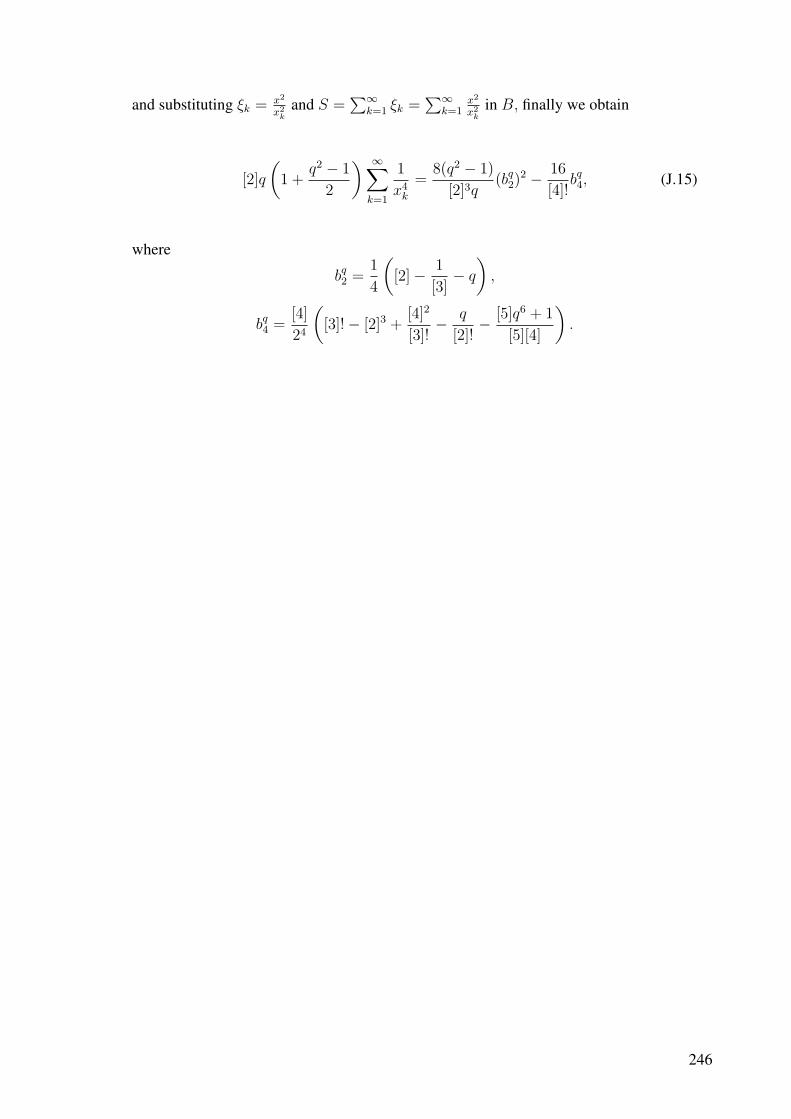
and substituting ξk = x2

x2k

and S =∑∞

k=1 ξk =∑∞

k=1x2

x2k

in B, finally we obtain

[2]q

(1 +

q2 − 1

2

) ∞∑

k=1

1

x4k

=8(q2 − 1)

[2]3q(bq

2)2 − 16

[4]!bq4, (J.15)

where

bq2 =

1

4

([2]− 1

[3]− q

),

bq4 =

[4]

24

([3]!− [2]3 +

[4]2

[3]!− q

[2]!− [5]q6 + 1

[5][4]

).

246