Embed Size (px)
Citation preview

Turning Point Tutors cc
Achieving academic excellence
Exam Revision Notes 2016 MSD 210Presenter 1: Wanga Mbasa

Table of ContentsIntroduction to kinematics.............................................................................................................................0
Concept definitions ..........................................................................................................................0
Four types of rigid-body plane motion ......................................................................................0
Angular velocity is the same at on any point on a rigid body ............................................1
Time derivative of a rotating fixed length vector.....................................................................................2
Relative velocity.........................................................................................................................................3
Relative acceleration.................................................................................................................................5
Rolling Wheel.............................................................................................................................................6
Chapter 4 Dynamics of System of Particles .................................................................................8
Generalization of Newton’s Second Law..................................................................................................8
Principle of Work-Energy...........................................................................................................................9
Principle of Impulse-Momentum............................................................................................................10
Conservation of Energy-Momentum.......................................................................................................13
Chapter 5 Kinetics of Systems of Particles...................................................................................................14
Steady mass flow......................................................................................................................................14
Steady mass flow system......................................................................................................................14
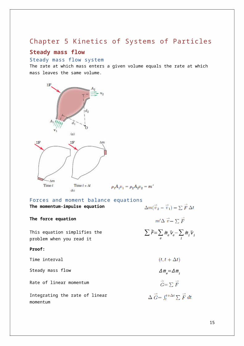
Forces and moment balance equations...............................................................................................14
Angular momentum-angular impulse..................................................................................................15
Chapter 6 Plane Kinetics of Rigid Bodies......................................................................................................16
General Equations of Motion...................................................................................................................16
The general equations of motion.........................................................................................................16
Reduced the system.............................................................................................................................16
Moment of all external forces about the centre of mass G.................................................................16
Alternative solution..............................................................................................................................17
Fixed rotation (Special Case)................................................................................................................17
Coupled rigid bodies.............................................................................................................................17
Analysis procedure...............................................................................................................................18
General Plane Motion..............................................................................................................................19
Rolling wheel............................................................................................................................................20
Translation................................................................................................................................................20
Fixed axis rotation....................................................................................................................................21
Work and Energy......................................................................................................................................22
Kinetic energy of a rigid body...............................................................................................................22
1

Work energy equation..........................................................................................................................23
Power...................................................................................................................................................23
Conservation of Energy-Momentum....................................................................................................24
PROPERTIES OF HOMOGENEOUS SOLIDS................................................................................................25
Chapter 8 Vibration of Single Degree of Freedom Systems.........................................................................26
Vibration of single degree of freedom systems.......................................................................................26
Equilibrium Position as Reference........................................................................................................26
Damped free vibration.........................................................................................................................27
Solution for Damped Free Vibration....................................................................................................28
The transient behaviour of single degree of freedom vibratory systems................................................30
Harmonic excitation.................................................................................................................................31
Undamped Forced Vibration....................................................................................................................32
Damped forced vibration.........................................................................................................................33
8/4 Vibration of Rigid Bodies....................................................................................................................36
Rotational Vibration of a Bar................................................................................................................36
Appendix B: Moments of Inertia and Products of Inertia............................................................................38
B/3 Parallel-axis theorem.........................................................................................................................38
B/7 The thin plate theorem......................................................................................................................38
B/9 The parallel-axis theorem for products of inertia..............................................................................39
2

Introduction to kinematicsNote: always work in two dimensions in dynamics
Concept definitions Kinematics is the branch of mechanics concerned with the motion of objects without reference to
the forces which cause the motion. Kinetics deals with the effects of forces upon the motions of bodies. A rigid body is a body in which deformation is neglected or the distance between any two given
points remain constant in time regardless of external forces exerted on itFour types of rigid-body plane motion
FIGURE 1: RIGID BODY PLANE MOTION

Angular velocity is the same at on any point on a rigid body
Define two lines on the body specified by angles with the horizontal axis.
θ1 for line1∧θ2 for line2
Let the angle between the two lines be β and because the body is rigid β remains constant
Thus , θ2=θ1=β
Thus if we differentiate θ1∧θ2 with respect to time θ1=θ2
Again if we differentiate θ1∧θ2 with respect to time θ1=θ2
All lines on a rigid body have the same angular displacement, same angular velocity and same angular acceleration.
1

Time derivative of a rotating fixed length vectorThis is used to prove that the velocity of a rotating fixed length vector is given by the angular velocity crossed with the vector itself.
Important to note:
r is a fixed length vector Rotation with the angular velocity of ω=ω k
FIGURE 2: TIME DERIVATIVE OF A ROTATING FIXED LENGTH VECTOR
e t=k ×er but limΔ t →0
et=¿ e ¿ e t is defined to be perpendicular to the z axis and the direction of the vector r . For an infinitely small time increment it is in the same direction as Δ r
˙r= limΔ t → 0
r|t+Δ t−r|t
Δt= lim
Δt →0
ΔrΔt
= limΔ t →0
r Δθ eΔ t
= limΔt →0
r ωΔt eΔt
Using maths we can reduce the expression to a simpler form
¿ r ωe=r ω ( k ×er )=ω× r
v=ω× r Thus for an fixed length vector the velocity is given by the following equation
2

FIGURE 3: THE VELOCITY OF A RIGID BODY ROTATING ABOUT A FIXED POINT
Relative velocity
FIGURE 4: RELATIVE VELOCITY
The above diagram is used to derive the equation for relative velocity.
r A=r B+r A /B Using the vector sum from the above diagram
vA= vB+ v A /B Taking the derivative of the vector sum
vA /B Is the relative velocity of point A as seen by a non-rotating observer at and moving with point B
r A ¿OA ¿ A−O
r B ¿OB ¿ B−O
r A /B ¿ BA ¿ A−B
Just a reminder from 1st year on vector notation
It is very important to understand what is meant by the observer for the relative term.
The relative velocity equation may be extended to a special case of relative velocity where points A and B are on the same rigid body.
3

Then the relative term may be represented as:
vA /B=ω× r A /B
And thus the relative velocity of A may be represented as:
vA= vB+ω× r A /B Just remember it is a special case
Visualizing the separate translation and rotation components of the equation help you understand the problem.
FIGURE 5: VISUAL REPRESENTATION OF THE RELATIVE VELOCITY EQUATION USING DISPLACEMENTS
FIGURE 6: VISUAL REPRESENTATION OF THE RELATIVE VELOCITY EQUATION USING VELOCITY COMPONENTS
A sketch of the vector polygon which represents the vector equation should always be made to reveal the physical relationships involved. The choice of coordinate system can greatly simplify the problem.
For rotations with constant angular accelerations:
4

Relative accelerationWe can derive the relative acceleration equation from taking the time derivative of the velocity equation.
vA= vB+ v A /B Using the relative velocity equation and taking the first time derivative
a A= aB+ aA /B We obtain the relative acceleration equation
a A /B Is the relative acceleration of point A as seen by a non-rotating observer at and moving with point B
Again the special case of A and B being on the same body is examined:
a A /B=ddt
[ω× r A /B]The relative acceleration term is found by differentiating the relative velocity term
¿ ˙ω× r A /B+ω× ˙r A /B Using product differentiation
¿ α × r A /B+ω× v A /B But from the velocity section we know thatvA /B=ω× r A /B
¿ α × r A /B+ω× ω×r A /B
¿ (a A /B )t+( aA /B )n Which represent the tangential and normal components or the relative acceleration term
5

Where
(a A /B )t=α × r A /B
(a A /B )n=ω×ω× r A /B
Rolling WheelThe rolling wheel has some properties that greatly simplify wheel problems.
FIGURE 7: ROLLING WHEEL RELATIVE VELOCITY AND ACCELERATION
The following assumptions are to be made:
Assume that there is no slip between the ground and the wheel. Assume that the centre of the wheel travels in the direction of the slope Assume a point of contact (point C) and thus vC=0 , (aC ) t=0, however (aC )n=ω× ω× rC/O and
is not necessarily zero
6

Relative Velocity
vO= vC+ vO /C Rewriting the relative velocity equation for the center or the wheel (Point O) and the point of contact (Point C)
vO= vC+ω×rO /C Since the wheel is a rigid body we can use the relative velocity term from our special case
vO=ω× rO /C Since the wheel is not slipping the point of contact (Point C) will have the same velocity as the surface it touches. In our case the ground thus vC=0
vO=rω This mean we are able to determine the velocity of the wheel center is the angular velocity is known or the angular velocity if the center velocity is known
Relative acceleration
aO=aC+ aO /C Rewriting the relative acceleration equation for the center or the wheel (Point O) and the point of contact (Point C)
aO=aC+ α ×r O/C+ω× ω×rO /C Since the wheel is a rigid body we can use the relative acceleration term from our special case
aO=−ω ×ω× rO /C+α × rO /C+ω×ω× rO /C However from our assumptions of no slip we have
(aC )t=0 and
(aC )n=ω× ω× rC/O=−ω×ω× rO /C
aO=α ×rO /C
aO=αr This mean we are able to determine the acceleration of the wheel center is the angular acceleration is known or the angular acceleration if the center acceleration is known
7

Chapter 4 Dynamics of System of Particles
Generalization of Newton’s Second LawThe most used part of chapter 4 is the notation on the figure below. You should be able to draw the diagram out of your head and know the labelling very well.
FIGURE 8: NOTATION FOR CHAPTER 4
O Is the origin
G Is the center of gravity (CG) of the body
P Is a random or arbitrary point used as a reference or observing point
i Stands for a certain particle of the body
r i Is the vector distance from the origin to the ith particle
rG Is the vector distance from the origin to the CG
r P Is the vector distance from the origin to the point P
rG / p Is the relative vector distance from the point P to the CG
ρi Is the relative vector distance from the CH to the ith particle
ρi ' Is the relative vector distance from the point P to the ith particle
In first year you learnt to calculate the center of mass:
rG=∑ mi ri
∑ mi
m rG=∑ mi r i=∑ mi( rG¿+ ρi)¿
m rG=r G m+∑ mi ρi
Thus
8

∑ mi ρi=0
This proof states that the vector sum of all the particles about the CG must be a zero vector.
Newton's second law as applicable to a system of particles:
Using Newton’s second law
Apply this equation to solve for the acceleration of a system of particles by using Newton's generalised second law.
Principle of Work-EnergyU 1−2 is defined as the work done by sources internal and external to the system
Work-energy equation:
U1−2=ΔT
Where
9

U 1−2' =ΔT+ ΔV
Where
V=V g+V e
U 1−2' =(T 2−T1)+(V 2−V 1)
The work done from state one to state two is equal to the change in potential and kinetic energy.
Use this equation when the work can be calculated or is asked for and the system has to states. It is also used to determine position and velocity of the system.
U 1−2' =Mθ Work done by a moment
U 1−2' =Fd work done by a force
1. explain what each term in the work-energy equation means
Principle of Impulse-MomentumLinear momentum is a quantity of motion of a moving body measured as a product of its mass and velocity. It can be thought of as the difficulty of changing the motion of a body.
Linear momentum of the representative particle of the system is defined as:
Using vector sums we can prove that the momentum for a system of particles is the same as the mass of the system multiplied by the velocity of the center of gravity, provided that the mass is constant.
Taking the time derivative:
10

Similar to linear momentum angular momentum may be defined. Angular momentum is defined for a system about the fixed point O, about the mass center G, and about an arbitrary point P.
The angular momentum about a fixed point O is vector sum of the moments of the linear momentum about O of all particles of the system.
Taking the time deriviate of this gives us:
The pairs of internal forces cancel out when all of them are summed.
Thus the resultant vector moment about any fixed point of all external forces on any system of mass equals the time rate of change of angular momentum of the system about the fixed point:
The angular momentum about the mass center G is the sum of the moments of the linear momentum bout G of all particles.
With the mass center G as a reference, the absolute and relative angular momentum are seen to be identical.
11

If we take the time derivative of the angular momentum about the point G:
The rate of angular momentum about G is equal to the sum of the moments of the external forces about G. These equations are some most powerful of the governing equations in dynamics and apply to any defined system of constant mass.
Next we investigate the angular momentum about an arbitrary point P. The absolute angular momentum about any point P equals the angular momentum about G plus the moment about P of the linear momentum of the system considered concentrated at G.
The proof:
Thus if we have the angular momentum of the CG we can determine the angular momentum of the system about any point and vice versa.
However we must remember that the rate of angular momentum about an arbitrary point P is in general not equal to the moments about the point P.
First we determine the moments about point P:
12

Now we determine the angular momentum about point P:
This is convenient when a point P whose acceleration is known is used as a moment center.
Conservation of Energy-Momentum “A mass system is said to be conservative if it does not lose energy by virtue of internal friction forces which do negative work or by virtue of inelastic members which dissipate energy upon cycling.”
If no work is done on a conservative system during an interval of motion by external forces (other than potential forces) then none of the energy of the system is lost.
U 1−2' =0∧thus 0=ΔT+ ΔV
0=(T 2−T1 )+( V 2−V 1 ) whereV =V g+V e
This implies that there is no change in energy to the system and is the “Law of Conservation of Dynamic Energy”.
The “principle of conservation of linear momentum” is defined for an interval of time where the resultant external force ΣF acting on the system is zero.
˙G=0∨G1=G2
Similarly for a fixed point principle of conservation of angular momentum is given as:
( HO )1=( HO )2∨( HG )1=( HG )2
13

Chapter 5 Kinetics of Systems of Particles
Steady mass flowSteady mass flow systemThe rate at which mass enters a given volume equals the rate at which mass leaves the same volume.
Forces and moment balance equationsThe momentum-impulse equation
The force equation
This equation simplifies the problem when you read it
∑ F=∑e
me ve−∑i
mi v i
Proof:
Time interval
Steady mass flow Δ me=Δmi
Rate of linear momentum
Integrating the rate of linear momentum
14
Note that the force needs to be constant for the interval
When using this term it is important use either use relative or absolute velocity, however never mix the two.
Volume flow rate:
Some time the question will provide volume flow rates rather than areas or entrance/exist velocity
V ¿=V out where Qis defined asQ=V
Q=Av
m=ρQ
Angular momentum-angular impulseFor steady mass flow about any fixed point O:
Angular momentum - angular impulse equation:
Moment equation:
Proof
∑ me' (de ×v e)−∑mi
' (d i × vi)=∑ M o
15

Chapter 6 Plane Kinetics of Rigid Bodies
General Equations of MotionThe general equations of motion- solve for the rotational and translational motion of a rigid body
Reduced the system- resultant force and moment:
Moment of all external forces about the centre of mass G
16

For 2D system:
two force or translation equations one moment or rotation equation
Remember parallel plane problems are also 2D problems
Alternative solution
+/- is determined by the sign of the moment created by m aG about point P.
Fixed rotation (Special Case)
Note if the motion is constrained (Kinematic analysis) or unconstrained (Kinematic chapter 5)
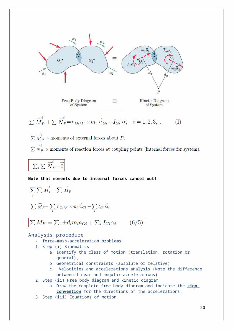
Coupled rigid bodiesThe system is defined by the boundaries set out. Sometimes it may be more convenient to analysis the entire system rather than individual components.
17

Note that moments due to internal forces cancel out!
Analysis procedure- force-mass-acceleration problems 1. Step (i) Kinematics
a. Identify the class of motion (translation, rotation or general), b. Geometrical constraints (absolute or relative)c. Velocities and accelerations analysis (Note the difference between linear and angular
accelerations)2. Step (ii) Free body diagram and kinetic diagram
a. Draw the complete free body diagram and indicate the sign convention for the directions of the accelerations.
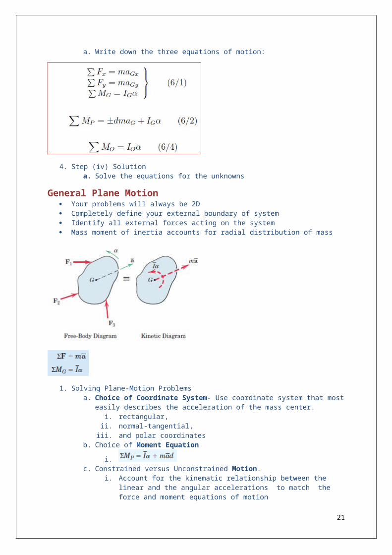
3. Step (iii) Equations of motiona. Write down the three equations of motion:
18

4. Step (iv) Solutiona. Solve the equations for the unknowns
General Plane Motion Your problems will always be 2D Completely define your external boundary of system Identify all external forces acting on the system Mass moment of inertia accounts for radial distribution of mass
1. Solving Plane-Motion Problemsa. Choice of Coordinate System- Use coordinate system that most easily describes the
acceleration of the mass center. i. rectangular,
ii. normal-tangential, iii. and polar coordinates
b. Choice of Moment Equation
i.c. Constrained versus Unconstrained Motion.
i. Account for the kinematic relationship between the linear and the angular accelerations to match the force and moment equations of motion
ii. Unconstrained motion- the accelerations can be determined independently of one another by direct application of the three motion equations
d. Number of Unknownsi. The number of unknowns cannot exceed the number of independent
19
ii. In plane motion we have three scalar equations of motion and two scalar components of the vector relative-acceleration equation (can solve for 5 unknowns per rigid body)
e. Identification of the Body or Systemf. Kinematics (Chapter 5 work)g. Consistency of Assumptions
i. Assumptions must be consistent with the principle of action and reaction
Rolling wheela. Slip
-a friction force is developed
F=μk N and a ≠ rα
b. No slip
- Same assumptions as in chapter 5 a=rα
Translation1. Rectilinear and curvilinear translation
a. It is important to note the angular velocities and acceleration are zero for translation
20
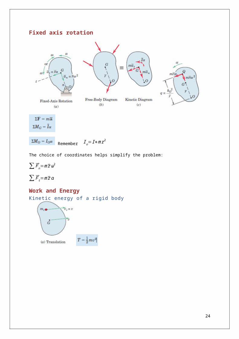
Fixed axis rotation
Remember I o=I +mr 2
The choice of coordinates helps simplify the problem:
∑ Fn=mr ω2
∑ F t=mr α
21

Work and EnergyKinetic energy of a rigid body
22

Work energy equation
U 1−2 is defined as the work done by sources internal and external to the system
Work-energy equation:
U1−2=ΔT
U 1−2' =ΔT+ ΔV
Where
V=V g+V e
U 1−2' =(T 2−T1)+(V 2−V 1)
The work done from state one to state two is equal to the change in potential and kinetic energy.
Use this equation when the work can be calculated or is asked for and the system has to states. It is also used to determine position and velocity of the system.
U 1−2' =Mθ Work done by a moment
U 1−2' =Fd work done by a force
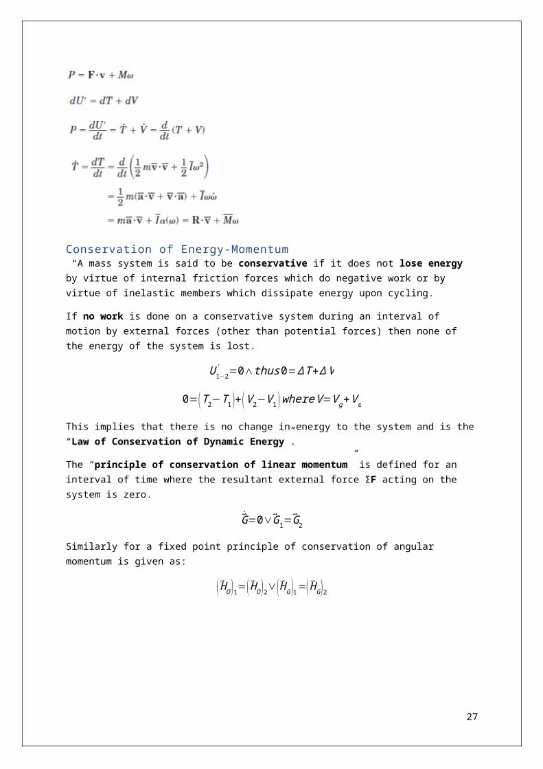
Power
23
Conservation of Energy-Momentum “A mass system is said to be conservative if it does not lose energy by virtue of internal friction forces which do negative work or by virtue of inelastic members which dissipate energy upon cycling.”
If no work is done on a conservative system during an interval of motion by external forces (other than potential forces) then none of the energy of the system is lost.
U 1−2' =0∧thus 0=ΔT+ ΔV
0=(T 2−T1 )+( V 2−V 1 ) whereV =V g+V e
This implies that there is no change in energy to the system and is the “Law of Conservation of Dynamic Energy”.
The “principle of conservation of linear momentum” is defined for an interval of time where the resultant external force ΣF acting on the system is zero.
˙G=0∨G1=G2
Similarly for a fixed point principle of conservation of angular momentum is given as:
( HO )1=( HO )2∨( HG )1=( HG )2
24

PROPERTIES OF HOMOGENEOUS SOLIDS
25

Chapter 8 Vibration of Single Degree of Freedom Systems Chapter 8 uses differential equations of motion, so that the linear or angular displacement can
be fully expressed as a function of time. We will investigate free and forced motion, with the further subdivisions of negligible and
significant damping. The damping ratio will be use to determine the nature of unforced damped vibrations. Harmonic forcing is driving a lightly damped system with a force whose frequency is near the
natural frequency can cause motion of excessively large amplitude—a conditioncalled resonance.
energy method can facilitate the determination of the natural frequency n in free vibration problems where damping may be neglected
Vibration of single degree of freedom systemsFree vibration-the disturbance of the equilibrium position of a spring mounted body resulting in the motion without the presents of any imposed external forces.
For an undamped free system the motions is sinusoidal since nothing acts to slow the motion.
Equilibrium Position as Reference
Newton’s second law
26
Equilibrium position Newton’s second law with equilibrium terms cancelled out The weight of the mass is balanced by the initial spring deflection. If we define the displacement variable to be zero at equilibrium we may ignore the equal and
opposite forces associated with equilibrium
Damped free vibrationWe start our analysis with damped free vibration:
Thus external force acts to excite the system The spring and damping force act as internal forces on the masses in the system
k-spring constant, modulus, or stiffness Spring force=−kx acts opposite to the displacement Damping force=−c x acts opposite to the movement
Applying Newton’s second law:
27

Natural frequency
o natural circular frequencyo ƒn=ωn /2π
viscous damping factor or damping ratio
o is a measure of the severity of the damping
o
Solution for Damped Free Vibration
Characteristic equation
Characteristic equation root:
General solution:
The systems damping ratio may be any valueThe radicant may be in one of three categories: Overdamped, critically damped of underdamped.
Underdamped system (ζ <1)The system will oscillate before settling.
Damped natural frequency
C∧ψ are determined for initial conditions x (0 )∧ x (0)
28

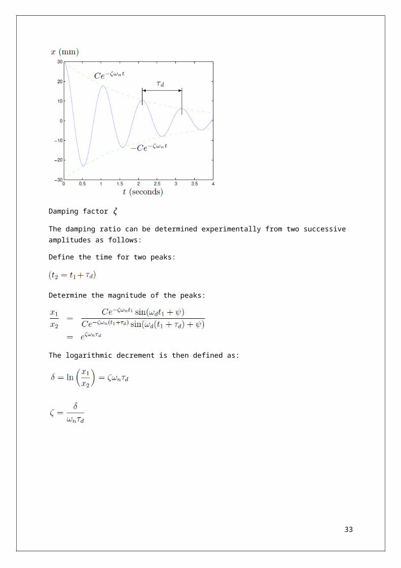
Damped period is defined as:
Damping factor ζ
The damping ratio can be determined experimentally from two successive amplitudes as follows:
Define the time for two peaks:
Determine the magnitude of the peaks:
The logarithmic decrement is then defined as:
29

Overdamped system (ζ >1) There is no oscillation and no period.
The magnitude slowly decays.
Critically damped system (ζ =1)
The amplitude approaches zero for long periods of time.
The transient behaviour of single degree of freedom vibratory systems
30

derive the equation for the calculation of the amplification factor and indicate what it is used for sketch graphs of phase angle and amplification factor against force frequency and indicate the effect
damping, rigidity and mass have on the response write down an expression for the total response of a forced single degree of freedom system Solve problems for forced systems.
Harmonic excitationForced vibration is a result of an externally applied force or may be generated motion of the base.
Some examples are illustrated below:
Forced vibration due to a force input:
31

Forced vibration due to motion of a body:
Undamped Forced Vibration
Newton’s Second Law of Motion gives the following equation of motion:
The solution to an undamped forced vibration problem is the sum of the complimentary solution and the particular solution.
xc = complimentary solution to the homogeneous equation (also known as the transient solution)
o x p = particular solution (also known as the steady state solution) The particular solution is required to have the same form as the excitation force
For example
If the particular solution is substituted into the equation of motion an expression of the ampl
32
The complete solution is given as:
The complimentary solution decays with time because of damping which will always be present. The amplitude X is of particular significance.
The amplitude ratio or magnification factor (M) which is the measure of the severity of vibration is given as:
It is important to notice that as the forced frequency approaches the natural frequency the amplitude ratio approaches infinity. Physically, this means that the motion amplitude would reach the limits of the attached spring, which is a condition to be avoided.
ωn is called the resonant or critical frequency of the system. When ω becomes close to ωn the result is
large displacement amplitude X, this is called resonance. For ω < ωn, the magnification factor M is
positive, and the vibration is in phase with the force F. For ω>ωn, the magnification factor is negative, and the vibration is 180 degrees out of phase with F.
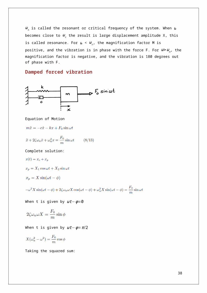
Damped forced vibration
Equation of Motion
33

Complete solution:
When t is given by ωt−ϕ=0
When t is given by ωt−ϕ=π /2
Taking the squared sum:
The amplitude is given as:
And the phase as:
Thus the general solution is rewritten as:
The magnification factor for a damped force vibration system
34

M = Magnification factor
ϕ= Phase angle
35

8/4 Vibration of Rigid BodiesRotational Vibration of a Bar
Step 1:
Horizontal position of static equilibrium. Equating to zero the moment sum about O yields
Step 2:
Arbitrary positive angular displacement
Step 3:
Parallel-axis theorem for mass moments of inertia
Step 4:
36

Simplify the problem Small angle assumption (state it if you use it):
oo
RHS=
.
37
Appendix B: Moments of Inertia and Products of Inertia
B/3 Parallel-axis theoremThe axes of C and G are parallel to each other and perpendicular to the plane.
Proof:
The origin is at G
B/7 The thin plate theorem
38

Equation of an ellipsoid
39

B/9 The parallel-axis theorem for products of inertia
40